.................! '- . .... ... .. . ... \7!0J - . . .DAVIDSON LABORATORY Report 1313 WAVE-I CE INTERACT ION by D. V. Evans and T. V. Davies D D-c Augl.lst 1968 tion of this document is unlimited • .. -- _.. ----_.. Reproduced by the CLEARINGHOUSE for Federal Scientific & Tecnnical . __ !nformation Springfield Va. 22151 :J' I W w

Welcome message from author
This document is posted to help you gain knowledge. Please leave a comment to let me know what you think about it! Share it to your friends and learn new things together.
Transcript

.................! '-. .... ...~. ..
£~).... \7!0J- . .
.DAVIDSONLABORATORY
Report 1313
WAVE-I CE INTERACT ION
by
D. V. Evans
and
T. V. Davies D D-c
s;ii~]-~
Augl.lst 1968
tion of this document is unlimited •. .-- _.. ----_ ..
Reproduced by theCLEARINGHOUSE
for Federal Scientific & Tecnnical. __!nformation Springfield Va. 22151
:J'I
W
w\\~

DAIJ I DSON L.ABORAiJ2(i
STEVENS INST lTUiE OF TECHhOLOGYCastle Point StationHoboken, New Jersey
Report 1313
August 1968
WAVE-ICE INTERACTION
by
D. V. Evans
and
T. V. Davies
Prepared for theOffice of Naval Research
Department of the Navyand
Supported by theArctic Research Project of theU. S. Naval Ordnance Laboratory
Contract Nonr 263(36)
(OL Project 3207/084)
DIstribution of thIs document Is unlImited. Application for copiesmay be made to the Defense Documentation Center, Cameron Station,5010 Duke Street, Alexandria. Virginia 2231~. Reproduction of thedocument In whole or in part is permitted for any purpose of theUnited States Government.
xiii + 102 pages1 table, 15 figures2 append ices
Approved J
S.~~--So Tsakonas, Chief
Fluid Dynamics Division

R-1313
ABSTRACT
-Three models are examined to study the transmls~!on ~f ocean waves
through an ice-field. In each case the effect of ice thjckn~ss. wate~
depth, and the wavelength and angle of incidence of t~'L ;~)coming O'~.;"~n wav~
is considered. In Hodel I the ice is assumed to consist of floating ~on
interacting mass elements of varying thickness and the shal1c",..-."ster
approximation is utilized to simplify the equations. A simpie ~osine
distribution varying in one direction only is assumed. In Model II •
mass elements, of constant thickness, interact through a bending stiffness
force so that the ice acts as a thin elastic plate. The mass elements are
connected through a surface tension force j~ ~odel III so that the Ice is
simulated by a stretched membrane. In b"Ul Models II arC. I; i the fl.l) 1
linearized equations are solved. Because of the complexity of the n·''i,:·t
Ing analysis, calculations of the reflection and transmission coefficit"~s
and the pressure under the ice, are made in Model lion the basis of th~
shallow water approximation.
KEYWORDS
Hydrodynami cs
Wave-Ice Interaction
Iii

R-1313
T ABLE OF CONTENTS
Abstract .. iii
Nomenclature •
Division of Stud!
v Ii
• x i I I
INTRODUCTION •..
Part
MODEL I. WAVE PROPAGATION THROUGH AN ICE-rIELD OFVARYING THICKNESS .... _ .. , ..
1.
2.
3.4.
Introduction and Equations Gov~r;':ln9 the Problem
Ice Thickness Varying in y-Direct:on withNorma 11 y Inc ident Waves . . . .
Modification for Obliquely '"eident Waves
Discussion of Results ...
5
5
7
14
16
(a) Existence of Energy Cut-Off and ItsDependence on the Various Parameters
(b) Numerical Results .
(c) Comparison of Results with Observation.
5 . Conc 1us ions. . . . . . . • . •
16
18
20
21
Part ! I
3. Method of Solution
i. Formulation
2. Preliminary Discussion of the Solution.
(a) Derivation of the Wiener-Hopf Equat :on
(b) The Far Field .(c) C",;·, rmi'1iit ion of J(O')
4. Relation Setw€'.m -j( ano r5. Shallow-Water Approximation
(a) Formulation and Solution
23
2326
Z92941
43
48
53
53[Cont'd]
WAVE TRANSMISS ION THROUSH A FLEX I BLEA. MODEL II.ICE-FIELD
v

R-13 13
Table of Co;:;!:~nts (Cont'd)
(b) Reflection and Transmission Coefficients
(c) Pressure on the Bottom, z -- 0 •..•
(d) Re lat ion Between '"'I!. and :::;- for Sha llow Water
(e) The Critical Angle in Shal::.:w Water
6. Discussion of Results.
(a) Description of Procedure
(b) The Critical Angle ...
(c) Reflection and Transmission Coefficients
(d) Pressure ~mplitude on the Bottom und~r the Ice
(e) Comparison of Results with Observation
B. MODEL III. AN ICE-FIELO HAVING SURFACE TENSION
I. Formulation and Solution
APPEND IX Po.
APPENDIX B
REFERENCES
TABLE 1. Frequency and Wa',e:length Bands Corresponding toIncident Waves Which are Completely Reflected
FIGURES (1-15)
vi
58
60
61
62
64
64
65
65
66
67
6969
77
81
85
87
.89-102

R-1313
NOMENCLATURE
Unless indicated, equation numbers refer to Part II of the report.
A
A.(i = 0,1,2}I
A••(i.j = 1.2)I.J
a
±iao
constant defined by Eq. (3.5); constant defined by Eq. (5.22)
constants defined by Eq. (5.25)
constants defined by Eq. (3.56)
constant in Mathieu's equation, defined by Eqs. (2.7)and (3.2) of Part I
pure imaginary roots of Eq. (2.1)
±a (n = 1,2,3 ... ) real roots of Eq. (2. I)n
±a Io
B
±ibo
constant defined by Eq. (2.2)
pure imaginary roots of Eq. (2.2)
±b (n = 1,2,3 ... ) real roots of Eq. (2.2)n
±b 'o
c
C', C"
..-c = ~gH
c.(i'" 1.2.3,4)I
path of integration for the integral in Eq. O.:n)
deformed paths of integration
constants defined by Eq. (3.30)
shallow water wave velocity
constants defined by Eq. (3.19)
vii

±c ±co 0
±c 'o
±c Io
R-1313
complex roots of Eq. (2.2)
D strip in the complex a-plane, - k < T < 0
D
E
F(x,y)
G(y)
9
g(~)
H
H(x)
h
h{x,y)
region T> k in the complex ~-plane
region T < 0 in the complex a-plane
Young's modulus for ice
defined by Eq. (1.8) of Part I
defined by Eq. (2.6) of Part I
acceleration due to gravity
defined after Eq. (3.53)
depth of water
solution of Eq. (1.10) obtained from separationof variables
constant ice thickness
mean and fluctuating ice thicknesses in Part I
variable ice thickness in Part I
vi i i

I
K
Ko
K Io
k
R-1313
coefficient of incident potential
wave number for incident waves in deep water
wave number for incident waves in shallow water
functions regul~r and non-zero in D~ respectively.defined by Eq. (3.25) and evaluated In Appendix B
{
wave number for undulations in the ice (Part I)
wave number for x-component of incident waves
k (nn
k •n
0.1 •... 5) roots of the equation
l
M
p
p
q
p.afhI
9
D/P9
coefficient in pressure fluctuation term. Eq. (5.38;
non-dimensional value of the pressure amplitude
water pressure
atmospheric pressure
constant in Mathieu's equation defined by Eq. (2.8)of Part I
ix

R
r
s
5
T
Ts
t
x,y
z
13'
y
e
eT
R-1313
coefficient of reflected potential
reflection coefficient
= T/pg
= Pi/p , specific gravity of ice
coefficient of transmitted potential
transmission coefficient
suriace tension force
time
horizontal space co-ordinates
vertical space co-ordinate
= a + iT., complex Fourier transform variable
constant defined by Eq. (3.10)
defined by Eq. (2.6)
angle between direction of incident wave and normal toice field
angle between direction of transmitted wave and normalto ice field
x

e .Crlt
A. .crlt
A .min
v
p
p.I
R-1313
critical angle at which complete reflection occurs
wavelength of incident wave
critical wavelength above which all waves penetratethe ice
minimum wavelength below which effectively no penetrationoccurs (Part I)
Poisson's ratio for ice
time dependent surface elevation
density of water
dens i t Y of i c.e
a real part of complex variable a
T imaginary part of complex variable a
~(x,y,z,t) time dependent velocity potential
Cp(x.y,t),0(y,z) shallow water velocity potential defined by Eq. (1.5)in Part I; defined by Eq. (1.9) in Part II, respectively
'P(o,z}
'i' 'i'+
Fourier transform cf V(y,z)
half-range Fourier transforms defined by Eqs. (3.14)and (3. IS)
ir(y,z)
w
ib 'y= :;(y.z) - e 0
wave frequency
cosh b zo

R- 13 13
DIVISION OF ST~JDY
The study is divided into two distinct parts. Part I ~onsists of
Model I, the propagation of waves through ice of variable thickness in
shallow water. This part is complete in itself, containing the analysis,
some numerical results, and a qu~litative discussion of the importance of
the various parameters in predicting wave transmission and reflection.
The main part of this work was carried out by Professor T. V. Davies,
Visiting Scientist, Davidson Laboratory, September 1965 to July 1966.
Part II contains Models I I ~nd I II, where the ice is assumed to have
a flexural stiffness and a surface tension-type force, respectively. For
Model II, numerical results for transmission and reflection coefficients,
together with the amplitude of the pressure fluctuation Qn the bottom
under the lee, are give~, together with a discussion of the results.
Eaeh part is ecmplete in itself and may be read separately.
xi i i

R-1313
INTRODUCTION
This reF~rt forms the theoretical part of a combined theo~etical
a:ld experimentel studyl5 into the effect of water waves on .an ice-field in
water of finite depth.
Wave transmission and refl~ction in finite and infinite depths of
water, partially ice-covered, have been the subject of a number of the')ret
ica] studies l ,2,3,4,5,6 in contrast to the scarcity of experimental ones. 7,8
The theoretical stlJdies have been dominated by the basic assumption that
the sheet of ice can be represented by a semi-inf;~ite rigid sheet, or by
a sheet composed of non-interacting floating polnt masses. So far, theory
reveals that the transmission of propagating undamped waves under the ice
depends upon the assumed surface condition, the ice thickness, the angle
of incidence of the incident waves, tha wavelength of such waves, and the
depth of water.
Heins l has assumed ~ne Tce to be a continuous rigid sheet without
movement, extended over a semi-infinite region ~f finite depth; he studied
the water wave-ice intel'ar.tion under the::;e conditions. Peters2 assumed
that the ice consisted of b"oken pieces with no interaction, i.e., neither
stiffness nor elasticity, extending over a semi-infinite region on the
surfa:e of an infinite depth of water; he found that there is a critical
inc idence freq'Jen';'/ wi',: ,:-; determines whether or not there wi 11 be a damped
transmitted \~ave ~;ter the interaction. Keller and Weitz3 have analyzed
the same problem, I)u'~ with water of finite depth. Shapiro and Simpson4
have made a numerical study of the abovp. reference which shows that water
waves entering an ice field are damped exponentially with increasing ice
thickness. Keller and Goldstein5 have considered the reflect .. 01 of water
waves from a region covered by floating matter ~ith and without surface
tension; they have solved the wave-ice interaction problem for an arbitrary
incidence angle by utilizing the shallow wate, theory. Their study rev~als
the importance of the incidence angle as well as of the degree of stiffness
of the floating material. Perhaps the most realistic model for the

R-1313
transmission of water waves by large floes is given by Stoke~6 although
his motivation was different. He was concerned with the effectiveness of
a floating beam having a known flexural stiffness, as a breakwater. The
treatment is restricted to two dimensions in the sense that the incident
waves enter the ice normally, and the shallow water approximation is
utilized.
Finally, the ob~ervations of Robin7,8 on wave propagation through
ice fields are considered to be fundamental in which he demonstrates the
existence of a higher cut-off wavelength depending on the size of floes,
above which no attenuation of water waves occurs, and a lower cut-off
wavelength below which the incident wave is comple:ely absorbed.
The present study consists of three distinct models. In the first
model the ice is assumed to be made up of floating non-interacting elements
of varying mass density distribution. The sh~llow water approximation is
used and a simple thickness distribution is considered to simplify the
analysis. A qualitative discussion is mad~ of the importance of the varia
tion in floe thickness, the angle at whi~h the incident wave approaches
the ice-field, the wavelength of the incident wave, and the depth of water.
It is shown that transmission of a given incident wave at a given incidence
angle is critically dependent upon the parameters of the problem, but that
waves which are long enough will always be transmitted into the ice. In
addition, some computations are made which indicate in effect a wavelength
~elow which no incident waves penetrate the ice. These results confirm the
observations made by Robin. 7
In Model II the i'ce (s assumed to have a constant thickness h, but
is allowed to bend tc permit the transmission of water waves. This corres
ponds to Stoker's model, but in this case waves may be incident on the ice
from any angle and the problem is solved for any depth of water H. Be
cause or the complexity of the analysis, numerical computations are made
only under the assumption of the shallow water theory. It is shown that
a critical incidence angle exists for each wavelength above which the
incident wave is completely reflected by the ice-field, without transmission
taking place. In addition there exists a critical wavelength above which
2

R-1313
all incident waves, at any incident angle, penetrate the ice-field as un
attenuated transmitted waves of reduced amplitude. Extensive calculations
are made which emphasize the importance of wavelength, incidence angle,
ice thickness and water depth, in determining transmission and reflection
coefficients, and the pressure fluctuations on the bottom under the ice.
It is felt that this model provides a good representation of the trans
mission of waves through large ice floes which, according to Robin,? have
been observed to bend to allow waves to propagate through.
In Hodel III the ice is assumed to be made-up of floating point
masses which are connected through a surface tension force. This model
was, in fact, considered before the more complicated Model II, and wcny
of the difficulties which arise in this more realistic case were first
encountered and solved in the simpler boundary-value problem of Model III.
It is acknowledged that this surface tension model is not a realistic
representation of the wave-ice interaction problem but it is of scone
academic interest since it extends the work of Keller and GoldsteinS to
finite depth of water. It is only given b~ief treatment since it follows
closely the techniques used in Model 'I.
3

~._- ... _------_. -BLANK" PAGE-:·· .
. .

R-1313
PART I
MODEL 1. WAVE PROPAGATION THROUGH AN ICE-FIELDOF VARYING THICKNESS
I. INTRODUCTION AND EQUATIONS GOVERNING THE PROBLEM
A semi-infinite sheet of ice of variable thickness is at the surface
of an ocean of uniform depth H ; the sheet occupies the domain 0 < y < ~ ,
- ..- < x < co Z = H and the remainder of the domain z H is open water.
O~ean waves are assumed to impinge normally on the edge of the ice-sheet
and the prob lem arises of the nature of the transmitted l·'ave. Here we
assume from Keller5 that the problem can be approached using the approxi
mations of shal low water theory, that is, we are as;;uming that the wavelength
It of the inc i den t ocean waves is long compared wi th depth H of water.
In the first place, if we approach the problem on the basis of the lin
earized theory only, the velocity potential ~(x,y,z,t) for the liquid
motion satisfies
and
2 +~ +<Pxx yy zz
o ,O<z<H (1. I)
2 = 0z z o (1. 2)
At the free surface of the ocean where ~(x,y,t) is the elevation above
the undisturbed level, we have, on the basis of linearized theory,
so that
2tt+g~z o z
5
H. -a><y<O (1.3 )

R-1313
The difference of pressure across the ice-sheet is given ~y
02p - Po'::!: P(d't - 9S)
and the equation of motion of an ice element, in the absence of bending
stiffness and surface stress effects, is
where Pi is the ice-density and h(x,y) the variable thickness of the
ice. Hence, the cond:tion to be satisfied on the ice-sheet will be
( 1.4)
where s = Pj/p 1s the specific gravity of ice.
In order to simplify the problem, we now invoke the shallow water
theory approximations and we do so by writing (see Keller5 )
( 1.5)
This expression will satisfy Eq. (1.1) to the first order and will also
satisfy Eq. (1.2). In order to satisfy Eq. (1.3), the function ~(x,y,t)
must satisfy
..m<y<o ( 1.6)
and, after some reduction of Eq. (1.4), w~ find that ~(x,y,t) must
satisfy
6

R-13 i3
Equations (1.6) and (1.7) constitute the basic equations of the
problem, the function h(x,y) being the prescribed var;able thicknes: of
thE: ke.
We can take the function ~ to contain the time throug~ . n exponen
ti~l factor, and if we write
~ = F(x.y) exp(-iwt)
then we have
ul~F +F +-F=O • -=<y<Oxx yy gH
and
{- sul} ul1 - -g- h(x.y) (F + F ) + - F = 0xx yy gH
,O<y<ex>
( I .8)
( 1.9)
( 1. 10)
At the boundary y '" 0 , it wi 11 be necessary to have ~ and ~y cont in
uous. expressing the continuity of normal and transverse velocity, hence
F , Fy
continuous at y o (l. 111
2. ICE THICKNESS VARYING IN y-DIRECTIONWITH NORMALLY INCIDENT WAVES
Here we take the ice thickness h to vary only in the y-direction
and, in order to simulate the effect of ice-floes, it will be assumed to
have the following structure:
h (2. I)
where hI $ ho and 2TI/k is the wavelength of undulations in the ice.
We look for solutions in which the incident ocean waves impinge
normally against the edge of the ice sheet, in which case the complete
expression for ~ in - ex> < Y < 0 can be taken to be
7
R-1313
(2.2)
where c =~. The transmitted wave in C < Y < c:c wi 11 be of the form
~ m G(y) exp(-iWt) (2.3)
and from (1.10) it follows that G(y) satisfies the differential eql;C1tion
sh wa sh u?{ (l- --2-.9) - _1_ cos kY} erG + u? G = 0
9 dy2 gH(2.4)
It is not necessary to work with this differential equation in the dbove
exact form since, when we insert typical value of the constants h ,hI'os , W , we find that
sh: 0..2
-«9
sh uta__0_«, g
for waves whose periodic time is greater than If s~conds and we shall
assume that the investi9atio~ is restricte~ to this class of waves. In
this case it is permissible to expand
in the form of a convergent infinite series in the parameter Sh1W2/(g-show2)
and thus to write (2.4) in the approximate form
u? sh lW"
erG of- gH {I + 9 cos ky} G = 0 (2.5)d7 sh W2 snow"(1- _0_) (1- --)9 9
8

R-1313
Accordingly, if we now write
Equation (2.5) becomes
ky = 21]
4,l~ Ia=~ ! _ sh;wa)\1
s~w2
21;;:- 9q = gHk" 2
~_ Sh;W
2
)
(2.6)
(2.7)
(2.8)
(2.9)
which is the stanci~rd form of the Mathieu differential equation (McLachlan,9
Theory and Application of Mathieu Functions). Periodic solutions of
Mathieu's equation e.dst only under special circumstances and in order to
make this clear we ref·er to the stability diagram in which q is the
abscissa and a the o~dinate (Fig. I).
If the values of q and a are such that the representative point
(q,a) in the stability diagram lies on the curves denoted by
there will be a periodic solution of Eq. (2.9). When q is sufficiently
small, it is known (see McLachlan) that the equations of ao ' b1
' a1
' •••
ore as follows:
(2.IO)
9
R-1313
4 1 a + 5 14. ( 8)b 2 = - 12 a 'i31rz'4 q + 0 q
4 5 2 763 14. O(.J3)a2~ + 12 q - T3S24 q + 'f
(2.11)
(2.12)
(2.13)
(2.14)
and the solutions corresponding to ao ' b~ , 81
in the usual notation
are as follows
a: ce (~)1 1
co
~ A(O) cos 2n~2no
.. co (1) (~ B2n+l sin 2n+l)~o
(2, IS)
(2.16)
(2.ll)
Elsewhere in the stability diagram the solution for G(Tj) of Eq. (2.9)
is of the form
(2. 18)
when~ !P(1J,IJ.) is a periodic function of 11, lJ.(c) is the characteristic
exponent of the Floquet-Poi~car~ theory, and cr is a parameter. We can
illustrate the significance of the parameter cr by considering first of
all, the area of the stability diagram lying between ao and b2
10

R-1313
Whittaker obtained the form of solution in this domain and he finds that
(Hc:Lachlan, p. 70) one soiution of i;2.9) is given by e1]~(cr) 4i(TJ.cr) as
follows:
and a and I.L are expressed in terms of q and cr ,~s follows:
a(o,q) I a 1 I= l-q coszcr+ '4 q (-1+ r Oslw )+ b4 cfcosza +
~(a.q) = - t q sin2cr + I~B cfsin2cr + ...
(2.20)
(2.21)
"IT!t will be noted that a(O,q) = 01 ' a(-"2 ' q) = a1 ' where b1 ' a1 are
thE values given in (2.11) and (2.12). Whittaker finds that the value
cr = - 1 n + i8 , 8 real , ~ 02
(2.22)
gives the region between a1
and ba and here ~ is purely imaginary.
This is therefore designated a stable area in the stability diagram.
In a similar way, the value
cr = ie, e rea I , ~ 0
gives the stable region between ao and D1
The area between
c; is such that cr is real and 1ies in the range1
b1
(2.23)
and
(2.24)
and this is designated an unstable area in the stability diagram. The
remainder of the stability diagram can be investigated and described in a
11

R-1313
'similar way.
The solution given in Eq. (2.18) indicates that the second solution
can be deduced from the above described solution merely by a change in the
sign of a.
Returning now to the wave problem. we see that as long as the
representative point (q,a) lies in any unstable domain (shown shaded in
the stability diagram), the corresponding solution for G(~) must be an
attenuated transmitted wave; the degree of attenuation will depend upon
the magnitude of ~(a) and we see that in Eq. (2.21). ~ will attain itsTT
maximum value in the unstable dc.marn (bI , ~) for cr = -"4 provided q
is sufficiently smal!. On th~ other hand. if the representative point
(q,a) I ies on a • b , a , b~ • ••• or within the stable unshadedo 1 I G
areas (ao ' bI
) • (a1
• b:a] , ••. , the solution for G(~) \":ill be an
undamped transmitted wave. The character of this undamped transmitted
wave will be periodic (but not a sine wave) when (q.a) actually lies on
the curves ao ' bl
• a1
• b:;) • '" ; the structure when (q,a) Ifes in a
stable area such as (ao ' b1
) is not periodic but almost periodic. This
description of regions of dampec and undamped solutions can be expressed
in a most useful form by returning to the definitions of a and q in
Eqs. (2.7) and (2.8). It will be noted that each of these parameters
contains the geometrical quantities H, ho ' hI ' the specific gravity
s as well as the wavel~ngth 2TT/k of the ice undulations and the ocean
wave frequency Piilrameter (1;; itwill be observed also that the parameter ill
when eliminated betwEOen i2.7) apd (2.8), leads to the relation
(2.25)
For a fixed value of (8/sk2 h1H) • this relation will be represented by a
parabola r. This parabola wi 11 intersect the curves b , a , b ,a1 1 :;) :;)
in points 61
, Al • B2
• A:;) •••. as shown in the diagram, and it is a
straight-forward matter to locate these points analytically when q is
not large. It is then possible to determine the values of ill at the
positions B.A.B,A ••••1 1 '2 2
which we can denote by
12
."

a
R-1313
""PARABOLA r"..
"..,/
SKETCH 1
It then follows that the domains of w defined by 0 < W< W(Bl ) ,weAl) < W< W(B2) , ••• lead to stable or undamped transmitted waves,
while the ranges
give damped or attenuated transmitted waves. The breadth of these ranges
will depend upon the parameter (8/sk2 hl
H) which is seen therefore to play
a crucial role. If we write
(2.26)
the parabola r has the equation a2- 2rq and the intersection of r
with the curve bl
, for example, can be obtained by combining (2.26) and
(2.11), namely
so that the intersection is given by
2rq (I _ q)2
13
(2.27)

R-1313
that is
q (l+r)-~r(2+r)
and the value of w then follows using (2.8). The approximate positions
can also be determined in this way.
To summarize the conclusions of this section of Part I, the impor
tant feature of the results is that when all the geometrical parameters
are fixed, namely, the depth of water, average ice thickness and departure
of ice thickness from the mean, the wavelength of undulations in the ice,
there can be certain wavelength ranges for the incident ocean waves which
will be attenuated on the ice-sheet and other wavelength ranges which will
be transmitted as undamped waves.
3. MODIFICATION FO~ OBLIQUELY INCIDENT WAVES
The above analysis requires modification whenever the incident wave
impinges upon the ice-field at an angle other than zero. In order to
carry out this modification, we refer to Eqs. (1.9) and (1.10). Clearly
the solution of Eq. (1.9) representing an incident wave making an angle ewith the ice-field is
iK Y cos e + iK x sin ee 0 0
where
and A is the wavelength of the incident wave.
Assume a solut ion of Eq. (1.10) of the form H(x) G(y) • Then sub
stitution into (1.10) gives
14

R-1313
where the thickness of the ice is assumed to vary in the y-direction only.
Since the left-hand side is a function of x only, while the right-hand
side is a function of y only, each side must be equal to a constant.
To obtain an oscillatory x-variation for all x, - ~ < x < ~ , it is
necessary that this constant be negative. Further, in order that the
solutions for y < 0 and y > 0 might be continuous at y = 0 for all
x , - ~ < x < ~ , it is necessary fer the x-dependence to be the same for
y > 0 as for y < 0 Thus
and
H{x} = eiKx sin e
o
Thus the equation satisfied by G{y) is
0.1)
Substituting the assumed thickness distribution hey) = h + h cos kyo 1
into Eq. (3.1) and making the same approximations as before, namely
gives
d2 G--- + (a + 2q cos 2~) G(~) 0drr
where in this case
4K :aoa =--
k21 - shK :a h
o 0
15
(3.2)

R-1313
2K <loq =--
k<l<l ;:
(l - sh K H)o 0
and the substitution ky = 21] has been made. Once again Mathieu's diffE'r
ential equation is obtained. Here also the frequency dependence may be
eliminated to obtain a relation between a and q , but since, in this
case, the relation is no longer simple, there seems to be no advantage in
doing this.
4. DISCUSS lON OF RESULTS
Ca) Existence of Energy Cut-Off And !tsDependence on the Various Parameters
The present mathematical model, based on the shallow-water approxi
mation, with ice undulations following a cosine distribution, clearly does
not represent an actual ice-field. However, a number of qualitative re
sults may be deduced which might be expected to hold true for more realistic
distributions of ice floes. Thus it has been shown that for fixed values
of k, h1
' H , there mayor may not be undamped transmission of a given
incident wave into the ice-field. By undamped transmission is meant a
wave travelling through the ice undiminished in amplitude with distance into
the ice. An attenuated transmitted wave is a wave which decays exponen
tiallyand travels only a short distance into the ice. Thus for e = 0
whenever the parabola given by Eq. (2.25) crosses a shaded region in
Fig. 1, the transmitted wave is attenuated, whereas when the parabola
crosses an unshaded region, the wave will be unattenuated and will proceed
through the ice. Thus the domains of w defined by
denote stable or undamped transmitted waves, while the ranges
J6

R-1313
denote damped or attenuated waves.
Now for shallow water, the relation between wavelength ~ and fre
quency w is given by
A = 2TT.J9Hw
so that corresponding to the domains of w described above we have the
wave-bands
denoting wavelength~ of incident waves which are transmitted through the
ice as undamped waves, and the wave-bands
A(B ) > ~ > A(A ) , ~(B ) > A> A(A ), •..1 1 2 2
corresponding to ~ttenuated transmitted waves.
One striking observation which may be made is that there exists a
wavelength
satisfies A > A(B) are1
the first energy cut-off
wave takes place for all
For A(B) < A < A(A) wave transmission2 1
and width of the stable and unstable
transmitted through the ice.
occurs and complete reflection
satisfying A.(A1
) < A < A(B1
).
again occurs. The distribution
such that all incident waves whose wavelength
When A = A(Bl
)
of the incident
regions are governed by the various parameters in the ~roblem, and it is
possible to make. the following gen~.al observations.
then
As h1~ 0 , corresponding to a uniform constant thickne~s
q ~ 0 and Mathieu's equation ciegeoprates i~to the p.quation
ho
17

R-1313
whose solution does not of course exhibit stable and unstable regions.
This may also be seen by considering the parabola
z 8a '" sk"'h H q
1
(8 0) 0.4)
For small h1
the parabola becomes steeper and the width of the unstable
regions becomes smaller, there being no unstable regions in the limit
hl
= 0 (see Sketch 1, p. 13 ).
A similar argument can be made for the case of small k, corres
ponding to long wave undulations in the ice, and small H, corresponding
to very shallow water. In each case the parabola (Eq. [3.4]) is very
steep and the width of the unstable regions are small, vanishing altogether
in the limit of H, k =O. This also follows from a consideration of
the I imit of the Eq. (2.5) for small Hand k
It appears from Eq. (3.2) that the effect of finite incidence angle
e is to reduce the value of a, while q remains constant, thus moving
points on the stability diagram into regions of greater instability. For
angles close to 90°, where a is close to zero. but still positive,
Sketch indicates that the first stable region 0 < W< W(Bl) is wide,
but that subsequent regions are predominantly unstable. Thus the wave
length A(B1 ) at which the first energy cut-off occurs is small, and
only narrow bands of wavelengths smaller than A(B1 ) penetrate the ice.
Further information concerning the effect of the various physical
parameters upon wave reflection and transmission was obtained by making
some computations which are described in the foll~wing section.
(b) Numerical Results
For the case of normally incident waves (6 00), some computations
were made to determine the breadth of the unstable regions corresponding
to complete reflection of the incident wave. Dimensions corresponding to
rr~del sizes were chosen which were then scaled using scale ratios of 80:1
and 200:1. Thus, ice thicknesses of ho = h1
'" 0.25, 1.00 and 2.00 inches
18

R-1313
were considered, with wavelengths of undulations in the ice (i.e., floe
length) of 0.50, 1.00, and 3.00 feet. The water depth was taken to De
0.50 feet and the specific gravity of ice s = 0.92. Then from Eq. (2.25)
the quantity a was determined for particular values of q The equa-
tions of the curves ao
' b1
' al
,ba up to be were computed using the
tables in Appendix I I of Mclachlan9 for q > 1 , together wit~ the series
expansions given by Eqs. (2.10) to (2.14) for q < I (see Mclachlan: p. 16
17). These curves were then drawn and the intersection of the parabola
za8
= ---;:r-hH qSK 1
with each curve a ,bl
, ... b , tabuiated. The intersection pointso 6
give values of q from which the frequency and hence the wavelength of
the incident wave can be determined using Eq. (2.8). These points which
span shaded regions (Fig. I) denoting unstable solutions of Mathieu's
equation, determine bands of wavelengths corresponding to incident waves
which are completely reflected by the ice-field. The results are given
in Table I. All wavelengths which lie outside the ranges indicated in
the table correspond to incident waves which are transmitted through the
ice as undamped waves. The largest wavelength given in each case is h(Bl
)
and all waves having a wavelength ~ > h(Bl
) propagate into the ice as
undamped waves.
From Fig. I, as q and hence, W increases indefinitely, the width
of the stable regions intersecting the parabola (2.25) diminishes until a
value of q is reached above which the bands of stable frequencies are
indistinguishable from points. Since the stability curves all cross the
real axis for large enough q (see McLac~lan,9 p. 39), the number of
intersection "points" is infinite. Associated with this value of q is a
wavelength which we denote by Amin Thus, we define ~min ' as the wave-
length below which the bands of stable wavelengths intersected by the
parabola CEq. [2.25]), are sensibly points, corresponding to very little
penetration of the ice. Clearly this is somewhat arbitrary, depending as
it does on the accuracy of computation, but A. does provide us with amin
19

R-13 13
useful bound below which only discrete wavelengths penetrate the ice-field.
Similarly, for small q. and hence w, the width of the unstable
regions intersected by the parabola (Eq. [2.25J) diminishes and reduces to
"points. 1I Also for large floes (k small), or thin ice (ho' h1
small) the
parabola is steeper and the bands of instability given by the intersection
are diminished.
In the tabie. both stable and unstable bands which are sensibly
points are omitted. As an illustrati~n of the use of the table, consider
the case of water of depth 100 feet, and ice of thickness 4.17 feet. Then
for floe lengths of 100 feet, A . = 162 there being no wave bands (butmIn
an infinity of wave "points ll) which penetrate the ice for A < 162 , "Ihereas
if the ice thickness is 16.67 feet, A. has more than doubled to 344.min
Also, note that all wavelengths penetrate a floe 600 feet long and 4.17
feet thick (apart from an infinity of discrete wavelengths) but if the
floe is 16.67 feet thick, there exists bands of wavelengths which fail to
penetrate the ice.
(c) Comparison of Results with Observation
A unique study of waves in pack ice was made by Robin7,8 during a
voyage into the Weddell Sea aboard RRS JOHN BISCOE in 1959-60. He finds
that for floes of around 1.5m thick and 40m or less in diameter,
1I ••• the main energy cut-off took place when floe diameterswere about one-third of the wavelength; little loss of energyoccurred when floes were less than one-sixth of the wavelength across, while no detectable penetration took placewhen the floes were half a wavelength or more in diameter."
From the table, the ciosest comparison can be made for floes of
4.17-ft thick and 100-ft long. Then little penetration takes place for
A < 162 corresponding to a floe length of five-eights the wavelength or
more as compared to the half wavelength observed by Robin?,8 It is not
possible to estimate the energy loss for long waves as this requires
knowledge of the transmitted wave amplitude and hence the full solution
of Mathieu's equation. However the table indicates that the first unstable
region corresponding to an energy cut-off or complete reflection of the
incident wave occurs when A drops to 248 feet or when the floe length is
20

R-1313
about two-fifths of the wavelenstr.. This compares favorably with the
observed value of one third of a ~~velength given by Robin. 7,8
5. CONCLUSIONS
It would appear that the simplified model considered here confirms
qualitatively the following observations of Robin:
(I) The existence of a critical wavelength at which a majorenergy cut-off occurs.
(2) The existence of a wavelength below which very littlepenetration of the ice-field takes pl~ce.
The one numerical comparison made shows surprisingly good agreement
of theory with observation. It would seem that a study of more realistic
thickness distributions would prove fruitful.
21

·, -"--- -------.~.-._-._.-----
BLANK PAGE. ;

R-1313
PART II
A. MODEL II. WAVE TRANSMISSION THROUGH A FLEXIBLE ICE-FIELD
J. FORMULATI O~
/ jC· c ./.--~=-::========::eI Az ~~~~I::S/ lLz~AVE
SKETCH 2
A semi-infinite ice sheet is floating on the surface of water of
constant depth H • A plane wave is obliquely incident from the region
- ex> < Y < O. Let ~(x.y.z.t) be the velocity potential of the liquid
motion. Then on the linearized theory of small amplitude water waves, ~
satisfies
~ + '" + ~ 0 O<z<Hxx yy zz
9! 0 , z 0z
~ + g<l> 0 at z ; Htt z
- ex> < Y < 0 (free surface)
let the equat ion of the ice field be
z = S(x,y,t) + H
23
(1 .2)
( 1.4)

R-1313
where ~(x,y,t) represents the displacements of the ice sheet above the
undisturbed free surface z = H Then Bernoulli's equation gives
and we also have
0<1'p(21t - 95) ( 1.5)
(1 .6)
on z = H , on the linear theory.
It is assumed that the ice sheet, having constant mass thickness h
is displaced from equilibrium by the differential pressure p - p , ando
that each element will be subjected to a force arising from the bending
stresses in the sheet.
It may be shown 10 that
where
and
jy4 S + p.h(S + g)I tt
0Eh3 E Young1s modulus
12( 1-\;2) v = Poisson's rat io
p. density of iceI
(1. 7)
Combining (l.S) and (1.7) and differentiating with respect to t gives
!P + gg>tt z
o IF cPp z
p.hI
P
24
z '" Ii O<y<o:> (1.8)

R- J3 J3
where (1.6) has been used.
Since the ice extends to infinity in either x-direction, it is
possible to subtract out the x-dependence. Assuming also a time harmonic
dependence of frequency w, let
p(x,y,z,t) = Re { 0(y,z)
whence 0(y,z) satisfies
ikxe
o a < Z < H (1. 10)
o~0 z = 0 - <to < Y < <tooz
K0o~ H ro < y < 0oz z =
K~o~ ( 0
2
k2y o~
(J-L) oz + M -- dz z = Holo < y <ex>
where K u} /g 2ITM== D/pg L
P i Kh==--r =--
p
(1.11)
(1.12)
(1.13)
Conditions (1.10) to (1.13) are not by themselves sufficient to give
a unique solution 0(y,z) Additional conditions regarding the vanishing
of the bending moment and shearing force at the edge of the ice field will
be imposed together with assumptions regarding the form of the solution
for y = ±"'. Assumptions concerning the behavior of 0 and its deriva
tives near y == 0, z = H which ensure that Fourier transforms converge
will be made during the course of the analysis. These assumptions may be
verified once the final solution is obtained.
Note that the particular case k == a corresponds to a plane wave
which is normally incident upon the ice field; that is, whose crests are
pa ra 11 e 1 to y = 0 .
25

R-I313
2. PRELIMINARY DISCUSSION OF THE SOLUTION
The eigenfunctions of Eqs. (1.10), (1.11) and (1.12) for y < 0 are
exp cos a z(n = 1,2, ••• ) where the a are then n
roots of the equation.
K cos a H + a sin a Hn n n o (2. J)
roots
K> 0
exp
wave.
y < 0
It is shown in Appendix A that there are an infinite number of real
a such that la I < la + I (n = ± 1. ±2 •••• ) and that forn n n 1
there are also two pure imaginary roots ± ia with eigenfunctionso,
[±y (k2 - a 2)"2J cosh a z. There are no other roots. For a planeo 0
k2 < a 2 so that there may be propagation in either y-direction for
o• since the exponent is purely imaginary. Thus for y negative,
the expected form of a bounded solution would be
1
exp [± iy (a 2 - k2 )2] cosh a z + 0 (exp ky)o 0
For y > 0 , the situation is more complicated. The eigenfunctions of
Eqs. (1.10), (1.11) and (1.13) are of the f~~m
I
exp [±y (k2 + b 2)2] cos b z (n 1.2, •.• )n n
where the b are the roots of the equationn
o (2.2)
A detailed examination of tne roots of this equation is made in Appendix A.
It is found that for L < 1M> 0 Eq. (2.2) has two purely imagi-
nary roots ± ibo • a doubly infinite sequence of real roots ± bn(n = 1.2, .•• ),
and four complex roots ± c ,± c (the assumption L < 1 covers the rangeo 0
of practical interest; the case L> 1 is not considered here). The exact
26

R-1313
ties in
c I > k0
c when0
b zo
which provide the wave propagation if
1,2, ..•),
exp 1%If Co I ~ cosh c z0
and
exp ~:l:Y cO' ~ cosh-c z
0
Thus for y positive, the expected form of a bounded solution would be
Re c I =o
exp~tiY (b0
2- k2)~} cosh bo
z + O(e- ky)
the terms O(e- ky) arising from the fact thatif b 2 > k2
0
Re - I > kc .0
the ice. This
If b <I < k2, then h . II b . .o t ere WI e no wave propagation Into
is made clear in Fig. 2. For the incident wave, we write
k = ao sin e and for the transmitted wave, k = bo sin 9T where ST
is the angle of transmission.
Then the incident wave is of the form
ia y cos e + ia x sin ee 0 0 cosh
whereas the transmitted wave takes the form
27
R-1313
iboY cos 8T
+ ib x sin 8T0 cosh b ze
0
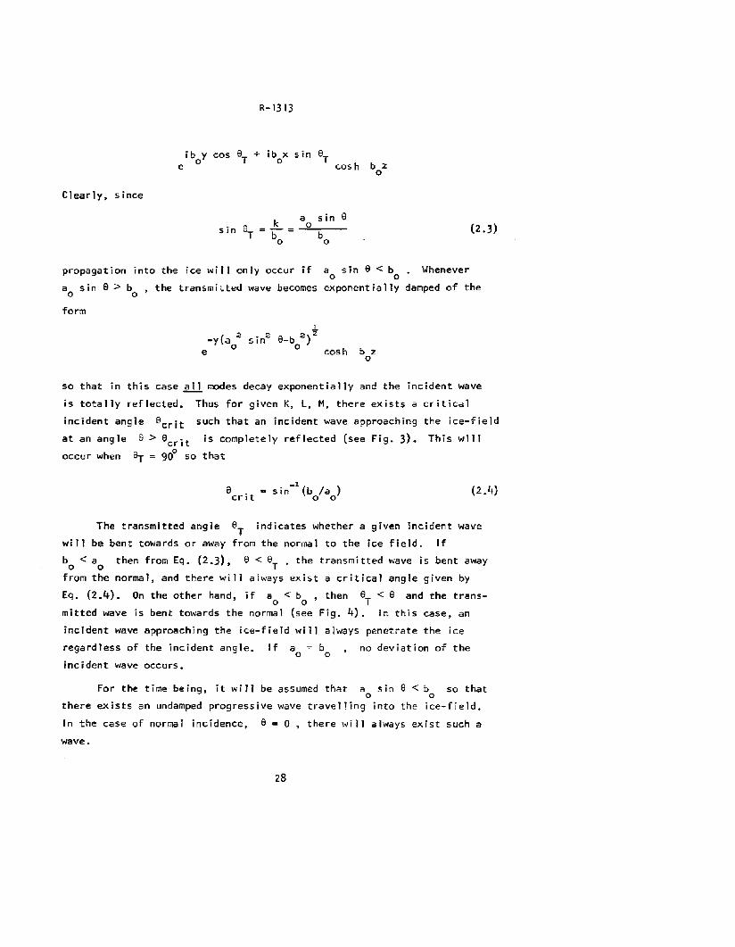
Clearly, since
ka sin 8
sin 8T
0= bo
= b0
(2.3)
propagation into the ice will only occur if a sin 8 < b Whenevero 0
ao sin e> bo
' the transmitted wave becomes exponentially damped of the
form
-yea aoe
~
6-b 2) 2o cosh b z
o
so that in this case~ modes decay exponentially and the incident wave
is totally reflected. Thus for given K, L, M, there exists a critical
incident angle 8crit such that an incident wave approaching the ice-field
at an angle 8> 6crit is completely reflected (see Fig. 3). This willooccur when 8T = 90 so that
_1 )e . = sin (b /acrlt 0 0(2.4)
The transmitted angle 8T
indicates whether a given incident wave
will be bent towards or away from the normal to the ice field. If
b < a then from Eq. (2.3), 8 < 8T ' the transmitted wave is bent awayo 0
from the normal, and there will always exist a critical angle given by
Eq. (2.4). On the other hand, if a < b , then aT < e and the trans-o 0
mitted wave is bent towards the normal (see Fig. 4). In this case, an
incident wave approaching the ice-field will always penetrate the ice
regardless of the incident angle. If a b no deviation of theo 0
incident wave occurs.
For the time being, it will be assumed that a sin 6 < b so thato 0
there exists an undamped progressive wave travelling into the ice-field.
In the case of normal incidence, 6 = 0 , there will always exist such a
wave.
28

R-1313
3. METHOD OF SOLUTION
(a) Derivation of the Wiener-Hopr Equation
The soluticn for the function fJ(y,z) is achieved by means of
Fourier transforms and the Wiener-Hopf technique. In order that the
Fourier transforms might converge in a strip of the transform variable
plane, the following device is used. The preceding section indicates the
expected form of the solution for large values of y. It is anticipated
that a prescribed oblique plane wave incident from y < 0 will give rise
to a reflected wave in y < 0 , and a transmitted wave in y > O. The
amplitude and phase of the reflected and transmitted waves are determined
once the incident wave is prescribed. However, we shall fix the amplitude
and phase of the transmitted wave beforehand and, hence, determine the
reflected and incident waves. The reason for this will soon become apparent.
Thus, let
£l(y,z)ibo'y
cosh b z + a(e-ky) o :5: z :5: H , Y > 0e0
1-<3. I)
where b r (b 2 _ k2 ) 2 and b ' b when k 00 0 0 0
and
where
+ia 'y - ia 'yO(e
ky).0(y,:z) Ie 0 cosh a z + Re 0 cosh a z +
0 0
a :5: :z :5: H , Y < 0
(3.2)
1
a I = (a 2 - k2) 2" and a I a when k 00 0 0 0
Division of the solution by I gives the solution due to an inciiao'y
dent potential e cosh a z .o
Consider, now, the function V(y,z) where
V(y,z) fJ(y,z) -
29
ibo'ye cosh b z
o

R-1313
Then from (3.1) Hy,z) is exponentially small for y> 0 so that
the Fourier transform of ,(y,z) with respect to y will exist in a
strip of the transform plane; a basic requirement for the successful appli
cation of the Wiener-Hopf technique.
Now, W(y,z) satisfies
where
*=0, z"O. -=<y<=
o~ ib~yKV = - + Ae , z = H , -= < y < 0cz
(3.4)
z=H.O<y<= (3.6)
'lr(y,z) y>o for each z (3.7)
y < 0 for each z (3.8)
It is assumed that outside some neighborhood of (O,H) wand its
first and second partial derivatives are also
O(e-ky) , y> 0 and 0(1), y < 0
30

R-1313
It is further assumed that W is bounded everywhere and that in a neigh
borhood of (O,H)
where
~oy 0<13<1 (3.10)
The reason for the assumption given by Eq. (3.10) requires some
explanation. There is no a priori reason why the velocity components
should be non-singular at the edge of the ice-field. Such singularities
invariably occur in potential problems at the confluence of two boundaries
on which different boundary conditions are satisfied. However, physically,
we require that there be no breaking of waves at the interface as this
would introduce an arbitrary constant to determine the amount of energy
loss which occurs. On a linear theory such a breaking phenomenon is
represented by a sink singularity in W so that the velocity components
would be 0(1) in the neighborhood of the leading edge, corresponding tor
the logarithmic singularity in W. By insisting that the singularity be
of the form (3.10), loss of energy due to breaking is just avoided, at
the same time allowing any milder singularity to occur in the analysis.
From conditions (3.9) and (3.10), the Fourier transform
...'i'(OI,Z) "1,,, ~(y.z)eiOYdy (3. II)
exists for 0 $ z $ H , and is regular for 0:' (= a + iT) in the strip
0: - k < T < 0 of the complex a-plane (see Sketch 3, p. 37). From
Eq. (3.3)
and integration by parts gives
<l i I"Nk $)e -'dy =0
'f (Q',z) =0
31
• (Q' e: 0 • 0 ~ z < H)

R-1313
1
Define y = (~ + k2 )2 such that the cuts extend from ± ik to ± i~
along the imaginary axis in the ~-plane. Then,
(i) As ~ = u (real) - 00 , y(u) ~ cr
(ii) Re (y) > 0 everywhere away from the cuts
and
The transform of condition (3.4) is
1 imz .... o
aVfaz(Ci.Z) = 0
so that A2(~): 0 •
From condition (3.10) it may be shown that
lim ~(~,z) = ~(~,H)
z-H-
and
Thus
limz-H-
0'£ o'i'oz (~,z) = oz (~,H)
and
'f (a, z) = If (a ,H) cosh yzcosh yH
o'foz (~,H) = yH tanh YH 'f (~,H)
(0' E: D)
(~ e D)
(3.12)
(3.13)
In order to obtain a Wiener-Hopf equation, the following notation is used.
Let
32

R-1313
where
...'i'+(a.z) ::: I Hy.z)eiCfYdy
o
exists for 0 ~ z ~ H and is a regular function of a
and
o'i'_(Q'.z) = f Hy,z)eiO'Ydy
-=
0.14)
in 0: T > - k+
0.15)
exists for 0 ~ z ~ H and is a regular function of a in 0: T < 0
Then
0'1± o'i'±lim ""z (a,z) - - (a,H)v - oz
z-H-
o'fIn future 'i'± (a,H) and 0; (a,H) will be abbreviated to 'f± and 'i'±' ,
respectively.
Now the transform of condition (3.5) is easily seen to be
K'I _ ::: 'I~ _ iAa + b~
(3.16)
Condition (3.6) is more troublesome. It is assumed that all y derivatives
f ~ ( H) d' I d' 05
~ ( H'o oz y, up to an Inc u Ing oy4 oz y, J are
It is also assumed that
is
33
y > 0
(0 < ~ < 1) as y - 0+
0.17)
<3.18)

R-1313
Then the transform of condition (3.6) exists and integration by parts
gives
+ y4 'i' I (0' eO)+ +
0.19)where condition (3.17) has been used, and where
02 [0 JCs = -a ~(y,H)oy y=O+
Thus the transform of condition (3.16) becomes
(0' € 0 )+
0.20)
Now add Eq. (3.16) to Eq. {3.20) and use Eq. (3.13). Then
lK cosh yH - Y (I - L + Hy4
) sinh "'l'H} '1'+' + ~ K cosh yH - Y sinh YHf'i'_'
= - Y sinh yH ~ 0' +i~o' + H [c4 -:O'CS - (~ + 2k.a)(~-iQ'Cl)Jf (0' e 0)
0.21)
Equation (3.21) is a typical Wiener-Hopf equation holding in a strip of
the complex O'-plane. Although Eq. (3.21) involves the constants c i (i=l,2,
3,4), it will be shown how 'i'l and hence ~ may be determined in terms
of just two constants.
Let
K cosh yH - Y(I - L + My4) sinh yH -= f (0')].
0.22)K cosh yH - Y sinh yH = f (0')
o
34

R-1313
Then
f1
- fo
= - (MY" - L) Y sinh'YH
and Eq. (3.21) becomes
It is shown in Appendix B that we may define
f (0') K (0')1 _ +~ ~ K (0')
o -
where K±(O') is regular and non-zero in D±, respectively.
it is shown that
K (0') O(a-2) 10'1 - 00 , (0' € I»+ ...
and
K_ (0') 110'1 - CD , (Q' € D)o( cfl)
Then (3.24) may oe written
0.23)
0.25)
Furthermore,
(3.26)
(3.27)
35
[
K (0') - K (- b I)J_ iA - + 0
0' + b 1o
(0' € D)
0.28)

R-1313
It is clear that each term on the left-hand side of (3.28) is regufar for
a € 0+ ' whereas each term on the right-hand side is regular for a € 0
Since the two sides are equal for a € 0 , this defines a function J(a)
regular for all (finite) a. The determination of J(a) is achieved by
a consideration of its behavior as laj - ~ .
Consider the left-hand side of Eq. (3.28). From (3.20), it is equal
to
(a € 0 )+
as,then J(a) = 0(a2 )
as 1011 -+ 00 in 0
as lal -+ CD in 0
in 0+
O(~)o(cil)
from condition (3.10), (see Noble,llo+
101\ -+ CD
K_(a)
, then J(a)in 0
in-+ 00
Now Y ,~I - 0 as laj - 00 in+ + .'.
p. 36, Eq. rl.74J).~
Thus, since K (a) = O(of) ,+
Simi larly, since
and Y I -+ 0 as
Hence
12Thus by an extension of Liouville's theorem, (Sec. 2.52).
(3.30)
Equating each side of Eq. (3.28) to
and adding, gives
J(a) , solving for Y I
+and Y I
~Note that this step is crucial to the ensuing argument. If we let e = 1in condition (3.10) inditatit'1g an energy source at the origin, then all wecan say is that ~+, f+ ' are bounded as 1011 -+ ~ in 0+ and in :he subsequent argument we find that J(a) = C of + r a + c. Then the solut iono "l zis no longer unique; the strength of the energy source at the leading edgeof the ice-field ~ust be given in order to determine the additional c01stant.
36

R-1313
from Eg. (3.13), this may be written in te,-ms of 'f. Thus,
(3.3 I)
or
(3.32)
Equation (3.12) and the Fourier inversion formula give
where C is some path in 0 as shown in Sketch 3.
SKETCH 3 t~Q;i 0 1 a-PLANEz
ti a:ik
I I I I I
~ ~uj-ik
-ib'I
• _I
-ico-ib'
2
-ib'3
37
--iel
o

R-13 13
The constants C1
and C2
will be determined from the ~onditions of zero
shearing force and bending moment at the edge of the ice, Z = H, Y = 0+ •
Assume for the ti~~ being that this has been done. Then it is ne~essary to
check that Eq. (3.33) with Y(a,H) , given by either Eq. (3.31) or Eq. (3.32)
does in fact satisfy the conditions of the problem. Now Y(a,h) is 0(0'-2)
as /0'1 - 00 in 0 so that the integral in Eq. (3.33) is uniformly con
vergent for 0 ~ z ~ H ,all y. Also, for 0 ~ z < H ,all y, the
integrals obtained by differentiating ~(y,z) with respect to y or z,
any number of times are also uniformly convergent. Since the operator0
20
2k2 I" d ,I. ( ) k h' d' h"d . IIoya + oz2 - app Ie to ,y,z rna es t e Integran vanls I entlca y,
it is ~Iear that condition (3.3) is satisfied for 0 ~ z < H ,all y.
Similarly, ~ondition (3.4) is seen to be satisfied on z = O. To verify
condition (3.5) for y < 0 , Eq. (3.31) is used in Eq. (3.33), and the path
of integration is deformed upwards in such a way that the ends of the path
tend to infinity along lines in the upper half-plane. It is now permissibleo
to ap~ly the operator K - az to W(y,z) and put z = H. Thus
0" 1f { iAK+(-b~) } -idy(Kljr- di) - - J(er) - :. (...) dO'z H 21T . a+b
O'"or "'"z: C1
where C' is the deformed path. It is clear that the only contribution
to the integral arises from the only singularity of the integrand in 0+
which is a pole at 0' = - bo ' • Thu~. for y < 0 ,
ib'y(Kt _ oW ) e Ae 0
OZ z=H
which verifies condition (3.5).
To verify condition 0.6) for y> 0 , Eq. 0.32) is used in Eq. (3.33),
and the ends of the path of integration are deformed downwards 50 as to
tend to infinity along lines outside 0 in the lower half-plane. Now for
y> 0 , it is possible to differentiate W(y,z) any number of times and
38

R-1313
put z H. Thus
{ a a'" .2 c;}K - (I-l) ~ -M(- - k:a) 00:- v(y,H)gz cy.2 Cz..
o
The boundedness of W(y,z) everywhere follows from the fact that W(y,z)
is given by a uniformly convergent integral for a ~ z ~ H , all y. A
differentiation with respect to either y or z produces an additional ~
into the numerator of the integrand so that the discontinuous part of the
integral behaves in a similar manner to
1'" -iay -a(H-z)
I = e e dO' ~ log r + bounded terms near z = H , Ya+1o
Thus, condition (3.10) is verified.
a
Condition 0.7) is verified by using Eq. (3.32) in Eq. (3.33) and
deforming the path of integration into the lower half-plap~, taking into
account the poles of the integrand. Since the singularity of the integrand
nearest the real a-axis is at a distance greater than k from it, it is
clear that V and also its first ar.d second partial derivatives are
O(e- ky) , for y> 0 and each z A similar argument may be used to
verify condition (3.8). In this case, contributions are obtained from
the poles of the integrand at
contributions of O(eky ) •
Q' = - b Io a = ± a I , together with
o
The conditions (3.17) and (3.18) require special attention. Now
0$ - I I(d'Z) z=H - 2iTc
39
-iaye ytanh YH

R-1313
where
and where the path C has been deformed so as to pass beneath the point
Q' = - ik. Write
y tanh YH = _1_ {K-Y(I-L)tanh YH _ l}K-y(1-L+Hy4)tanh yH My4 K-y(J-L+My4 )tanh yH
Then is regular and tends to zero in 1m (a) < - k • 50 that
Thus
where the integrand is O(~) as 10'1 ~ ~ in D.
a3 0,11It is clear that all y derivatives up to and including ~ 3(~}
uy oZ Hare bounded for y ~ 0 , and deforming the path of integration around
the poles of the integrand indicates that all derivatives are O(e- ky )
for y> o. It may be shown in a similar manner to the verification of
condition (3.1) that
0(109 r) r~ e y2 + (Z_H)2 near r = 0
Thus conditions (3.17) and (3.18) are verified, and W(y,z) does indeed
satisfy the condi~ion5 of the problem.
40

R-1313
(b) The Far Field
In order to demonstrate the form of the solution for large y, it
is convenient to use series representation of the solution.
Thus, for y> 0 , the integral expression (3.33) may be written
in terms of a sum of the residues at the poles of the integrands (see
Appendix B). Thus,
-cly2Fl (-i cl)e 0 e eose z eose H
VCy,z) c ...;...._...;:o~__.::.o_-......:o'--_-::o'-- _
c,f 2c H(1-L~Hc 4)+(1-L"'SHC 4)sin2c H\_(-ic l )d... 0 0 0 o~ 0
2Fl(-iel )eCOYc cose z cose H
+ 0 0 0 0
elf 2c H(I-L+Me 4 )+(1-L+5Mc 4 )sin2c H\ (-iel)oL 0 0 0 0:.1- 0
-~n=l
For y < 0 , similarly,
-bly2F.
i(-ib!)e n b cos b z cos b H
n n n n
b'[2b H(I-L+Mb4 )+(1-L+5Mb4 )sin2b H1K (-ib ' )n n n n n~- n
V(y, z)ib 'y
- e 0 COS" b zo
-ialy ia'y2ia cosh a z cosh a H r Fl(a~)e
0 F1 (-a~)e0
0 0 o , }~
a l (2a H+ sinh 2a H) ~
K+ (a~) K (-a")o 0 0 + 0
b'y2F1 ( i bn') e n b eos b z cos b H
n n n
41
n=1 b'[2b H+ sin2b HJn n n
(3.36)

R-1313
Comparison of the coefficients in Eqs. (3.35) and (3.36) with the
coefficients R and I occurring in Eqs. (3.1) and (3.2) indicates that
and
ia I (2a H + sin h 2a H)000
2a cos h a Ho 0
(3.37)
(3.38)
The reflection coefficient ~ is defined as the ratio of the amplitude of
the reflected wave to the incident wave at infinity. The transmission
coefficient r is defined similarly.
Now
os (oil)ot = oz z=H
so that the elevation S is given by
{I o~) i kx-iillt}
~(x,y,t) = Re ~(~ el~ oz z=H
Thus the elevation of the incident wave is
{a sinh a H ikx+ia'Y-iwt}r:( ) _ 0 0 0
~ x,y,t - Re . I e. IW
with ampl itude
a sin;I 0
w
42
a Ho
(3.40)

R-13l3
Similarly the amplitude of the reflected wave is
a 5 inh a HIRI .....:o~_----=o"OJ
The elevation of the transmitted wave is
(3.41)
~ b sinh~(x,y,t) = Ret 0 iOJ
b Ho (3.42)
with ampJ itudeb sinh b Ho 0
OJso that the reflection coefficient is
since
IF1 (a~) IIF~{-a~)1
and the transmission coefficient is
(see Append ix B)
b si nh b Ho 0
aosinh aoH1 al(2a H+sinh 2a H)sinh b H
_ 0 0 0 0
~ - a a 5 i nh 2a Ho ~
(c) Determination of J(a)
IK+(-a~)1
IF1(-a~)1
(3.44)
There are still two conditions which need to be satisfied at the
leading edge of the ice before the solution is uniquely determined. These
are conditions which express the fact that no energy is put in or taken
out of the system at the leading edge of the ice-field. A derivation of
these conditions is given by HiJdebrand. 13 They are
43

R-l3l3
where
(3.45)
(3.46)
is the transverse shearing force along y
is the twisting moment along y = 0
is the bending moment along y = 0
o
We have
and the conditions (3.45) and (3.46) in terms of S, become
02 ell! :>Ill( £.') k"' (UU\ = 0-2 "d'Z =H - v dZ'J z=Hey z
03
e~ 0 ail-3("""OZ)Z=H- (2-v) k
300::-(-) = 0 •oy oy CZ z=H
• y = 0+
y =.0+
C3 .47)
C3 .48)
These conditions, in turn, may be written in terms of V(y,z). Thus
;bob~sinh baH [b~2+(2-VW"J
ibob~sinh baH [bo2
+(1-V)k2]
<3.49)
44

R-1313
and
bo sinh boH ~o:a - (l_v)k2] y = 0+
(3.50)
In the case of normal incidence, k = 0 , and tne conditions on ~ are just
03 of/l';2"(,:,z)oy z=H
o , y 0+ (3.51)
2P ail~(oz)
y z=Ho y = 0+ (3.52)
which compare with Stoker6
Now if the expression (3.35) for Hy,z) is differentiated with
respect to z we obtain, for z = H ,
where
-b1yF
1(-ib)e n g(b)
n n(3.53)
and
g(fl)2(K cos flH + ~(!-L) sin flH) cos flH

R-1313
Remember that
iAK (- b .)+ 0
(Q'+b I)o
The conditions (3.49) and (3.50) when applied to (3.53) give
+ t {b~2 -vk2
)F1 {-ibn)g (bn) '" basinh boH [ba2
_(I_V)k2]
n"'lC3 .54)
Now
iAK (- b I)+ 0C
2+ C
1Q' - _.....:...._-=-
Q'+b Io
where
A ~ 'Mb 4 - L) b sinh b H\ 0 0 0
(3.55)
Clearly, there exist two equations for the determination of C1 and C2
•
After some algebra they may be written in the form
B1
(3.56)
46

R-1313
where
A =11i e; ,2
oic ,,,,
o
<Xl
-i ~n=1
b ,2 [b ,2 _ (2-\.1) k2 J g(b )n n n
(3.57)
C I rc ,2 _ (2-\.1) k2 J g(e; ) + c ' [C ,2 _ (2-\.1) k"'J g(e )o 0 0 0 0 0
<Xl
+ ~ bn '
n=1(3.58)
B = - ib b' sinh b H rb 2 - (7-\1) k2
] - AK (- b '>1, :~.b ' [c 12
_(2_\l)k2 J g(e;
1 0 0 0 0 + 0 e;o I 0 0 0
C I <Xl b I fo r- 1
2( ) 2J (-) '"" n [b 1
2 (2 )k2) (b)+ '=c-;-'-+~ib-;' Co - 2-\.1 k g e;o + L..i b ,+ ib I n - -\I g n
o 0 n=1 no)
- i
CXl
I:n=1
b '(b ,2 - \lk"') g(b )n n n
(3.60)
<Xl
+ I:n=1
47
0.61)

R-1313
b sinhbHfb"-(I-v)k"]000
(3.62)
Once C1 and C., have been determined, the solution of the problem is
complete and, in particular, the expressions (3.43) and (3.44) for the
reflection and transmission coefficients may be computed.
Unfortunately, the determination of the co~stants C1
and C., above
presents enormous computational difficulties, ;~volving as it does the
complex roots b of the transcendental equationn
K cos b H + b (l-L + Mb 4) sin b H 0n n n n
Thus, whereas the solution to the full linear problem has been obtained,
it will be necessary to resort to the shallow-water approximation to
derive the solution in a form more suited to computation. It is possible,
however, to derive a relation between ~ and ~ which will be done in the
following section.
4. RELAT ION BETWEEN 'IZ AND rJf'
Although the expl icit determination of 1<. and 1"' presents enormous
computational difficulties, it is possible to derive a simple analytical
relation between ~ and ~, by an application of Green's theorem. We
have seen that the two-dimensional function 0(y,z) satisfies the follow
ing conditions (Eqs. i.IO-I.13).
48

R-1313
~=o. 2=0. __ <y<:oOZ
oilKR!=..,....z=H • ..m<y<OOZ
Oil 0'" -., 021KRl = (I-L)~ + M(-2 -k"') OZ. Z = H. 0 < Y < ...
OZ oy
(4.1)
(4.2)
(4.3)
(4.4)
Also ~ is continuous and satisfies the conditions (3.47) and (3.48).namely
y = 0+ (4.5)
Green's theorem applied to the functions ~(y.z) and its conjugate
0{y.z) may be written
z- -:2 o~ - oR!S'r (RlV D- ~'V f1)dydz = l{fj ..,- - Rl -)ds"s c On On
(4.6)
(4.7)
where S is the area of the rectangle formed by the lines z = 0 , Z = H
and y =:Yo' C is the boundary of this rectangle, and n denotes the
normal directed to the exterior of the boundary. Since 0 and hence 0
satisfy Eq. (4.1), the left-hand side of (4.7) vanishes and the equation

R-1313
reduces to
1m I ~ o~ ds: 0C dn (4.8)
It is assumed that y is so large that for y = ±y • ~(y,z) may beo 0
replaced by its asymptotic form as given by Eqs.(3.1) and (3.2). Thus
ib I y~(y ,z) ~ e 0 0 cosh b z
o c(4.9)
+la I ycosh a z + Re 0 0
ocosh a z
o(4.10)
Now the contribution to Eq. (4.8) from z = 0 vanishes by virtue of Eq. (4.2).
Also, Eg. (4.3) implies that the contribution from z = H , - = < Y < 0
vanishes. Thus Eq. (4.8) becomes
Yo - H o~ H o~1m I ~ oil(y,H)dy + 1m S(0..,-) dz-Im ICll~) _ dz" 0 (4.11)
o az 0 oy y=yo 0 oy Y--Yo
The first t~rm presents the most difficulty, so this will be left to the
last. Substituting the asymptotic form for 0 into the second integral
gives
Similarly for the final te~m in (4.11), we find
:-1 -ia'y' +ia'y' +ia'y' -ia1y.
JI ( 0 0 0 0)(.- 0 0 - 0 0 a-1m -ia~ I e + R e \1 e - R e cosh aoH dz
o
a I
a 40 (2a H + sinh 2a H) (111 2- /R/ 2
)a 0 0
o
50

R-1313
The first term in Eq. (4.11) may be written
M YO~:a a -
f ,0 ;; a~ aRl(y,H) dyIII K l;:2 - k) az oz -- -
o oy
where Eq. (4.4) has been used, ard
Yo ~ -Im I~ 0.0 0.0 d 0
J OZ oz Yo
It is possible to integrate this expression by parts twice to obtain the
following result
MYo ~;; .:a o~ -~1m - f (-'"- - k2
) ~. ?1.J dK ~:a OZ' ,;;z Yo 0Y
". 1m !!K
where all the integrated terms \-Iere I:'lJrely real and hence vanished when
the imaginary part was taken.
Now the fir$t term vanishes at y = 0 from condition (4.6) and the
second term in brackets is seen to be purely real from Eq. (4.5) and so
it also vanishes. The value of this expression at the top limit Yo may
be determined, after some algebra, to be
.,.Mb I b .3 5 i nh 2b Ho 0 0
I-L + Mb ...o
Combining the contributions fro~ each of the terms in Eq. (4.8), we find
that
51

2b H°
I-L + Mb 4o
This may be written
b '_...2-.. (2b H + sinh 2b H)
4bo 0 0
a '+ 4~ (2aoH + sinh 2aoH) (11/ 2
- IRI~) 0o
b I 4Mb 4 ] a'
bo 12b H+sinh2b H(1+ 0) _1_ =~ (2a H + sinho 0 0 l-L+Mb 4 lIra ao 0
o
Now from Eqs. (3.43) and (3.44),
and
'R,:a2a H)(I -~)
° II/:a(4. 12)
~b 2 5 in h 2 b H
_1_° 0
2 sin h 2 a H 111 2a° °
b sinh 2b H0 0-
a sinh 2a H (l-l+Mb 4) Irl 2
0 0 0
so that in terms of~:a and Pe2, Eq. (4.12) may be written
where:
a 2 b l [(I-L+Mb 4 )2b H/sinh2b H+ (l-L+5Mb 4)]D =~ • ...!?.. ~__...::.o_--=o;.,-.__...::.o .:::o--=:....
b:a a' [ ]o ° 2aoH!sinh2aoH + 1
52
(4.13)
(4.14)

R-1313
The Case M == 0
In this case
[ 2b H
~o +
a ::I b ' si nh 2bo
H0 0 0 ( l-L)==b::li\ [ 2a H
~o c o +si n h 2a
oH
where
(4.15)
so that
K == a tanh a Ho 0
Kl-L
b tan h b Ho ()
a ::I b 'o == ....Q...--9-.
a 'b ::Io 0
(4.16)
which agrees with th~ value obtained by Weitz and Keller.3
5. SHALLOW-WATER APPROX I MAT ION
(a) Formulation and Solution
It is clear that the full solution of the linearized problem presents
overwhelming numerical difficulties and it is desirable to examine the
solution on the basis of the shallow-water approximation. Instead of con
sidering the limit of the "finite depth" solution, it is desirable, for
the sake of clarification, (and cer~ainiy ea~ier) to rederive the solution
from the original approximate equations based on the shallow-water theory.
We return to the Eqs. (1.1), (1.3), and (1.8) satisfied by the
velccity potential ~(x,y,z,t) •
il +2 +2xx yy zz o 0< z < H (5.1)

R-1313
4> 0z z '" 0 (5.2)
9 + g9 = _ ,g 1*9 _.E.L h ~ • z = H • 0 < Y < <Xl
tt Z P z P ttz
- <Xl < X < <Xl (5.4)
We have seen that additional conditions at the leading edge of the ice-field
are given by the equations
21 2I2 S; a2 s; + (I_v) 03 1;0oy (ay2 + Oxg) oy2lx2 '"
~ 02S;0+ V
Oy2 2Ix2
z '" H , Y 0+ (5.5)
z = H , Y = 0+ (5.6)
where S(x,y,t) is the elevation of the ice. These equations ensure that
no energy is put in or taken out of the ice at the leading edge. As before,
it is convenient to write
~(x,y.z.t) = Re {~(y.z)eikx - imt}
so that ~(y.z) satisifies
(5.7)
o < z < H • _CIO < y < 0 (5.8)
00 .. 0oz • z = 0
54
(5.9)

R-1313
z = H, -~ < Y < 0 (5.10)
, Z=H,O<y<CD
z=H ,y=o+
(5.11)
(5. 12)
_03 00 ( . 2 0 :::.m(-) - 2-v;k - (~)Oy3 oz oy oz
0, z=H, y=o+ (5. 13)
In employing the shallow-water approximation the potential 0 is ex
panded in powers of z, and it is found that
1 2( ~ )w( y) - - z ¢ - k'" ¢2 yy(5. 14)
satisfies Eqs. (5.8) and (5.9) up to order Z3. A precise derivation14of the theory is given by John who concludes that the theory is valid
provided the depth of the water is sma11 compared to a wavelength a~d to
the minimum radius of curvature of any immersed l-ody. If the expression
(5.14) for ~(y,zJ is substituted into (5.10) and (5.11), it is found
that W(y) satisfies
o _Cl> < y < 0 (5.15)
",here
55
o O<y<co (5.16)

R-1313
2
K 2 = K/H = IlL ,o gH
in terms of .(y) the conditions (5.12) and (S.13) become
o ,y 0+ (5.17)
O.y=O+ (S.18)
In addition, from the shallow-water approximation •
Hy) and ..tiMoy are continuousat y = C
(5.19)
iK I y -iK ' yNow the Eq. (5.15) has the solution W(y) = e 0 + Re 0 where
1
K I = (K 2 _ k2 )2 and the positive square root is taken. and K > k foro 0 0
a progressive wave. The form of the solution is such as to represent an
incident wave of prescribed amplitude, and a reflected wave of (complex)ik I y
amplitude R. Eq. (5.16) has a solution of the form e n where
.1.k I = (k 2 _ k2) 2
n n
and the k (n = 0,1, ... 5) are the roots of the equationr.
Mk 6 + (I-L) k 2 = K 2n n 0
(S.20)
(5.21 )
This equation is a cubic equation in k 2n
having solutions
56
(S.22)
(Cont'd)

R-1313
(5.22)
where1/2] 1/~
(1 + 4( l-L)3)\ 27MK 4
o
(5.23)
1/3 [ 1/2] 1/3
B = (Ko2
) I _(I + 4P_L)3),2M 27MK 4
o
(5.24)
and
2Trj /3e (- I +.J3i ) /2
In all cases of practical interest
A+B>O.
L < 1 and4{ l-L)3
27MK 4o
< I so that
Thus k 2 is real and positive while k/ = 's2 •o
is chosen such
is required
isiko'Y
e
y-+ '" .solutions. The
k I = (k :3n n
y > 0 a soluticn
The square root in the expression
that k I = k when k = o. Now forn n
repres~nting a progressive wave. Clearly such a solution
Other solutions are permitted provided they are bounded as
Energy considerations exclude the possibility of unbounded
only possibilities are those roots k which have positive imaginary parts,ikn'y n
so that e decays exponentially for increasing y. There are two1
:3 -such roots. ,Thus let k1 = + (k1 )2 have a positive imaginary part. Then
k;a = - (k;a:3)2 also has a positive imaginary part, since ~ = - Is .Hence the solution for y > 0 may be written
Hy)ik ' y ik1'y ik 'y
=Ae 0 +A1e +Ae:2o :2 (5.25 )
57

R-1313
The unknowns are the complex constants Ac
' Al
, ~ and R, and
there are just four conditions to be satisfied by W{y) . Since wand
oW/oy are continuous at y = 0 • then the following equations must hold.
1 + R
K '(I - R)o
(S.26)
(S.27)
Also, conditions (S.ll) and (5.18) give the equations
2
L fk/2 - (l_v)k2
] A. 0 (5.28)I
i=O
2
L: k il k. 2 fk. 2 + (1_v)k2 ] A. 0 (5.29)
I I I
i=O
which together with Eqs. (5.26) and (S.l7) are sufficient to determine
the unknowns. The problem .ls so 1ve,j once the constants Ao ' ~,A2 and R
have been computed, and expressions may be derived for physical quantities
of interest.
(b) Reflection and Transmission Coefficients
The transmission coefficient is the ratio of the amplitude of the
transmitted wave to the amplitude of the incident wave at infinity.
Now for large positive y,
iko1yV(y) - A e
o (5.30)
since the other two terms in Eq. (5.25) decay exponentially with increas
ing y. The elevation S{x.y,t) satisfies the Eq. (1.6), namely
<".......58

R-1313
z H
and in terms of V(y} the elevation may be written
( ){
iH 2 ikx + ikQy- itrtf~ x,y,t = Re -- k A ew 00
and the corresponding amplitude is
(5.31)
Hk :2o
UlIA Io (5.32)
The incident wave is given Wcident wave is
iK 'ye 0 so that the elevation of the in-
"H 2 e ikx + iK~Y. - iwt}~(x,y,t) = - Re {l- Kw 0
(5.33)
with amplitude ~ K :2 Note that this term contains the dimensional unitUl C>
amplitude of the incident wave and hence it has the correct dimensions.
Thus the transmission coefficient ~ is given by
(5.34)
and in a similar manner, the reflection coefficient 12 is given by
(5.35)
59

R-1313
(c) Pressure on the Bottom, z ; 0
From Eq. (1.5) the pressure on the bottom in excess of atmospheric
pressure Po is
(o~)p ; p + pgHot z=Q
(5.36)
In terms of the shallow water potential W(y) , we have
p(x,y,O,t) = p Re {_iw~(y)eikx - iWt} + pgH (5.37)
If the local effects represented by the exponentially decaying terms in
volving A1 and ~ in Eq. (5.25) are ignored, then the ampl itude of
the pressure fluctuatio~ on the bottom under the ice is
~ i kx + i ko I Y - i I.lJt lp(x,y,O,t) - pgH = Rei Pe ~ (5.38)
where Ipi pl.lJ IA Io
It is convenient to non-dimensionalize this in terms of the amplitude of
the incident wave. Thus we define
f IPI waIA I IA I;--
eKo)
HK a 0 09 0
pg ----w-
since K a = wa /gH •0
Hence Q7 is a measure of the absolute value of the amplitude of the pres
sure fluctuation on the bottom z; 0 , under the ice, compared to the
amplitude ofz:he pressure fluctuation on the bottom under the free surface.
60

R-I313
(d) Relation Between 1(. and '7 for Shallow Water
The Eqs. (5.26), (5.27), (5.28), (5.29) which determine the coeffi-
cients R and A conceal the relation existing between i'E: and rr.0
This is most eas i Iy de; ived by taking the 1imit for sma 11 H of the rela-
tion which has been derived on the basis of the full linear" equations.
From Eq. (4.13) we have
where
as
b 'oaro(l-L+Mb 4)2b H/sinh2b H + (1-l+5M b0
4 )J" 0 0 0
so
H _ 0
o - (l-l + 3Mb 4)o
where b is the real positive roots of the equationo
K = b 2 ( 1-L + Mb 4) Ho 0
since tanh b H~ b H(I + O(b h)2.o 0 0
This equation may be written
where
61

Clearly bo - kosame basis
R-1313
in the shallow-water notation and b Io
k I. On theo
Thus
K = a 2 H so that a - K and a I K Io 0 0 0 0
K:a k I
o - ....2.......2... (l-L + 3Hk 4)2 K I 0
k 0o
and for shallow water
If we introduce the incident angle e and a transmitted angle aT by
writ ing
k = K sin ao
then the above formula becomes
This relation will provide a check on the computed values of ~ and ~.
(e) The Critical Angle in Shallow Water
As in the case of finite depth of water, the constant k in theikxx-variation e determines the angle at which the incident wave enters
the ice-field. Thus if we write k = K sin e , then the incident wave iso
of the formiKoY cos a + iKox sin a
e
62

R-1313
so that the incident wave makes an angle e with the normal to the leading
edge of the ice-field. as shown in Fig. 2.
The reflected wave is of the form
-iK Y cos e + iK x sin eo 0
e
indicating that the angle of incidence is equal to the angle of reflection.
The transmitted wave has the form
1
i (k 2 K 2 sin2 8)2" y+ iK x sin e ik cos aTY + ik sin 8Tx
0 0 0 0 0e - e
where k :a satisfies0
sin a kMk 6 + (I-L)k 2 K :3 and 0 (5.40)
0 0 0. s in aT =i(
0
and above which
k is real, there willo
(Assuming l < I.) But if
then there will exist a
e = 0 • sin a = 0 • and sinceClearly when
always exist an undamped transmitted wave.
for particular values of M and l K >• 0
critical value of 8, at which k 2 = K 2100
(k 2 _ K 2 S in2 8)2 is pure imaginary, thus producing an exponent iallyo 0
damped transmitted wave. This value of a is given bye. = sin-1(k /K ).crIto 0
An incident wave approaching the ice at an incident angle greater than
8 . will be totally reflected by the ice as shown in Fig. 3.crlt
On the other hand. if k > K then (k 2 - K" s in2 e) is alwayso 0 0 0
positive. so that waves approaching at any angle will penetrate the ice.
rn this case the transmitted wave is bent towards the normal so that the
ice may be regarded as being "denser" than the water. When K = ko 0
which, from Eq. (5.40), occurs when MK 4 = l , the transmitted wave pro-o
ceeds at the same angle as the incident wave. The waveiength at which
this occurs is denoted by "crit and hence any wave satisfying A > Acritpenetrates the ice regardless of the incidence angle.
63

R-1313
6. DISCUSSION OF RESULTS
(a) Description of Procedure
In obtaining the numerical results. the following values. taken from
Robin. 7 were used
Young's modulus for ice E = 5xl01o dyn!cmz
Poisson's ratio for ice v = 0.3
Now
Density of ice
Density of sea-water
p. = 0.92 gm!cm3
I
p = 1.025 gm/cm3
and
2TTKo = T ' so that
Robin7 has observed ice thicknesses of about 1.S metres so that values of
h 0.75. 1.5. 3.0 metres were considered together with water depths of
H 10, 20 metres. The incidence angle e was allowed to vary in steps of
150 from 0 to 60°. and various wavelengths of the incident wave. up to
700 metres. were considered.
In each of these cases. the Eqs. (5.26), (5.27). (5.28). and (S.29)
with coefficients determined from Eqs. (5.22). (5.23), and (5.24) were
solved and values were obtained for ~.~. and ~.
In addition, the critical angle e . above which an incident wavecn tis completely reflected and the critical wavelength, A .t above whichcnan incident wave at any angle penetrates the ice. were computed in each
case.
As a check on the numerical work, the expression
64

R-1313
was evaluated. This should, of course, from Eq. (5.39) be identically
zero. The fetct that this expression was, in all cases, negligibly small
provided a check on the numerical accuracy as well as a verification of
the shallow-water approximation since the relation between or and 1f!was derived by taking the limit for small H of the corresponding result
based on the exact linear theory. Presumably this same relation could be
derived directly from the analytic solution of the equations determining
A and R.o
The results are shown in Figs. 5 through 15.
(b) The Critical Angle
In Fig. 5, the critical incident angle is shown as a function of
incident wavelength. The critical angle determines whether or not a given
incident wave at a given' incident angle is able to penetrate the ice (see
Figs. 2 and 3). Thus a wave approaching the ice-field at an angle egreater than the critical angle (as determined from Fig. 5) is completely
reflected by the ice field. If the incident angle is less than e 0tcr I
then penetration of the ice field occurs and an undamped transmitted wave
travels through the ice field. Incident wavelengths greater than ~critn
corresponding to 6crit = 2 will always penetrate the ice, regardless of
the incident angle (see Fig. 4).
(c) Reflection and Transmission Coefficients
Figures 6 to 10 show the variation of f( and ~ with the incident
wavelength Ie for ice thicknesses of 0.75, 1.5, and 3.0 metres, incident
angles r3nging from 00 to 600 in steps of 15°, and water depths of 10 and
20 metre~.
In ~ig. 6 the curves for l' have been extrapolated so as to pass
through the origin. This is not strictly accurate since at Ie = 0 , L
is infinite, and it has been assumed that L < I • There does in fact
exist a cut-off wavelength (unrelated to the incident angle) which occurs. 4(L-l)3
whenever Eq. (5.21) fails to have a real root. ThiS occurs when 27MK 4 >
and then all possible solutions in the ice-field decay exponentially 0
with distance. This restriction is of little physical significance since,
6S

R-1313
for example. with h = 1.5 metres. H = 10 metres. no propagation is possible
for A < 10-4 cms. approximately. In other words. this mathematical phenom
enon only occurs at wavelengths too small to be physically significant.
Figures 6 to 10 illustrate the importance of ice thickness in deter
mining reflection and transmission. Thus, for instance. from Fig. 6.
doubling the ice thickness from 1.5 to 3 metres causes a drop of over 25%
in the wave amplitude of the transmitted wave corresponding to an incident
wavelength of 250 metres. Since the wave energy is proportional to the
square of the wave amplitude, this means almost a 50% reduction in energy
caused by doubling the ice thickness.
In contrast. the water depth has little effect on the reflection and
transmission coefficients except for the smaller wavelengths.
As would be expected. the ability of the ice to reflect the incident
wave is reduced as the incident wavelength increases, and for A > 500 metres.
the transmitted wave height is at least 95% of the incident wave height.
In all cases. the amount of reflection was very small except for the lower
wavelengths. This agrees with the conclusions of Stoker,6 who considered
the two-dimensional problem (e = 0°).
Figures 6 to 10 furthermore indicate the effect of the angle of
incidence upon the reflection and transmission coefficients. For a fixed
wavelength there appears to be a gradual increase in transmission with
increasing incident angle. For a given incident angle ~,- decreases until
the cut-off wavelength is reached. at which l' drops to zero and complete
reflection occurs. For larger incident angle a distortion of the trans
mission curves takes place so that. for example. when e = 600• the trans
mission curve for ice of 3 metres thickness has a minimum at a wavelength
of about 320 metres.
(d) Pressure Amplitude on the Bottom Under the Ice
Figures 11 to 15 show the variation in non-dimensional pressure
fluctuations ~n the bottom under the ice normalized with respect to the
pressure on the bottom in the absence of ice. in terms of the incident
wavelength A • ice thickness h , water depth H, and incident angle e.
66

R-1313
In all cases the pressure amplitude 00 tends to unity as A in
creases, which is to be expected. For e = 0°. the pressure is generally
lower than the corresponding pressure amplitude on the bottom in the ab
sence of ice, the pressure drop being greater for greater ice thickness.
For e = 15°, considerable changes in the pressure curves take place and
for the lower incident wavelengths 00 is actually greater than unity for
an ice thickness of 3 metres. This trend increases for larger values of
e so that for e = 60° the pressure jumps to over 1.5 the free surface
bottom pressure in the most extreme cases. As in the case of the trans
mission coefficients, for each non-zero angle there is a cut-off wavelength
corresponding to e "t at which the pressure drops abruptly to zero,crl
indicating complete reflection of the incicent wave.
(e) Comparison of Results With Observation
Robin7 has concluded that no effective transmission of wave energy
occurs for wavelengths less than 200 metres in fields of large floes,
whereas major energy changes occurred in those waves having a period of
16 seconds, or wavelengths of 400 metres.
It is difficult to compare observations in deep water with a theory
based on the shallow water appr"oximation. Thus Figs. 6 to 10 indicate
that energy transmission through the ice occurs at much lower wavelengths
than v;".:erved by Robin? For instance, when A = 100 metres, h = 3.0m,
~= 0.3 indicating that over 9~1o of the incident energy has been trans
mitted into the ice. This discrepancy is almost certainly due to using
the shallow-water approximation. If the numerical difficulties involved
in the solution based on the full linearized theory could be surmounted,
it is felt that a much closer comparison of theory and observation would
result.
The experimental counterpart of this wave-ice investigation is re
ported in Ref. 15.
67

. .. .0. •__--___ ._...•
I BLANK" PAGE·• . t

R-13l3
B. MODEL III. AN ICE-FIELD HAVING SURFACE TENSION
I. FORMULATION AND SOLUTION
In this model it is assumed that each element of the ice sheet is
subjected to a force arising from a surface tension force in the sheet.
Then it may be shown that
p - p = - T ifl s + p. hso S I tt
where T = surface tension force.s
The theory proceeds exactly as for Model II except that the free
surface condition satisfied by V becomes
(6.1)
where S = Ts/pg .
z H,O<y<c:o (6.2)
The characteristic equation is
K cos b H + b JI-L-Sb 2 t sin b Hn n1 n~ n
o (6.3)
which has an infinite sequence of real roots ±b (n = 1,2, ••• ) and twon
pure imaginary roots ±ib , for K,S > 0 , L < I Thus propagation alwaysooccurs in the ice, if Ib I > k. Also, complete reflection of a planeoincident wave will always occur for some angle of incidence wheneverL < Sa 2
o
The transform of condition (6.2) is obtained by integrating by parts;thus
K'l' = 'i' I ( 1-L + S-t) + S (a - i eta) (et e: 0 )+ + 2 1 +
69
(6.4)

R-1313
with the same notation as before. Similarly, for y < 0
K'i' = 'i' I (O! € 0 )
Following the same procedure as in Model II, we arrive at the equation
(6.5)
'" J (a)
(o:eD) (6.6)
where
KcoshYH-y(I-L+Sy2)sinhyH
KcoshyH-ys inhyH .
and 1St(Q') is regular and non-zero in D±, respectively.
The left-hand side of (6.6) is regular everywhere in D+ while the right
hand side is regular everywhere:n 0 • The two sides are equal in the
strip 0 . This deflnes a function J(Q') regular in the whole Q'-plane.
It may be shown that
K+(c.') '" O(a)
K_(Q') ;:; O(Q'-I)
IQ'I - '" in D+
1c.'1- ... in D
Furthermore 'i'±' = 0(1), la/ - 00 in D±, as in Model I I.
But the left-hand side of (6.6) is just
K(a) {K~ - '1' .}+ + + IK (Q') - K (- b ,)I- i A. + + 0 = J (a)
a + b Io
70
(6.7)

R-1313
and so J(~) = o(~) as I~l - ro in 0+.
Similarly from the right-hand side of (6.6)
J(~) = o(~) , as J~I - ro in 0
Thus from an extension of Liouville's theorem
J(~) C, a constant
We find from Eq. (6.6), that
'f(~,H)
and so
C - iAK (- b I)+ 0
~ + b Io
1 s<O cosh'VzV(y,z) = 211 Y(o-.H) h H-= cos .'V
where the path of integration is in 0
We see that the solution depends upon a constant C. An additional
condition is required to determine C.
The required condition is obtained by applying Green's theorem to
the functior ~(y,z) and its complex conjugate ~ in the rectangle formed
by the lines z = 0 , z = H , y = ± Yo. Note, by analogy with Model II,
that ~(y,z) satisfies
(2 :l 2 2C Icy + c IOz )~(y,z) ~ 0 (6.8)
, z=H, -= < Y < 0
71
(6.9)

whereu?
K =-9
R-1313
K6 t= (l-L)~!L s(~ _k 2 ) ~ .z9-l. 0 < Y < CDOZ Oy2 Oz
Pi h'J)2 TL=--,S=2
pg pg
(6.10)
where
ib'y~(y.z) '" Teo coshboz + O(e-ky). 0 ~ z ~ H. y> 0
ia~y -iaby ky~(y.z) a I e coshaoz + R e coshaoz + O(e )
O~z~H.y<O
(6.11)
(6.12)
and
1
a' '" (a 2 -k 12
o 0
K cosha H a sinha Ho C 0
K coshb H b (l-L+Sb 2) sinhb Ho 0 0 0
The method is identical to that used in Model II to determine the
relation between 1<. and q-. In addition, it provides us with the
required conditions for the potential at infinity to be unique.
Green's theorem reduces to
1m J ~ ~ ds (6.13)C
where the line integral is taken over the boundary of the rectangle. The
contributions from z = 0 and from z H, - ~ < Y < 0 vanish, and the
contribution from z = H, 0 < Y < 00 is
72

R-1313
The contributions to Eq. (6.13) from the boundaries y = ± Yo are
and
-b' (2b li+sinh2b H) ITlao 0 0 . 1~ , respect Ive y
o
Thus combining all the terms, and using the relation
Ksinh2b H~ i nh2 b H = -..::.0__
o 2b (l-L+Sb a)o 0
we obtain
Now from Eq. (6.14), if 11/ 2 == 0 , so that no energy is being
supplied to the system, R = T = 0 if and only if
73
(6. 14)

R-1313
2 -m(o ~ o~) = 0
I dYdZ dZ" z=H -y=O+
(6.15)
This condition must therefore be satisfied to ensure that no energy is
being supplied to the system other than by the incident wave. Then the
following relation may be derived between the reflection coefficient
and the transmission coefficient
where
a 2 b l [(1-L+Sb 2 )Zb H/sinhZb H + (1-L+3Sb 2)1o =~~ 0 0 0 0 ~
. b:3 a l [2a H/sinh2a H + 11o 0 0 0 'J
When H is small, this reduces to
in the notation of the shallow-water approximation used in Model II.
The condition (6.15) may be satisfied in more than one way and the
74
(6.16)
(6. 17)
(6.18)
(6.19)
(6.20)

R-1313
physical unreality of the model does not provide an obvious choice. How
ever, the tension existing in the ice sheet, z H, y> 0 suggests there
must be a restraining force at the edge of the sheet y = 0+. For instance,
if the ice is fixed at that point in some way such that the elevation is
zero, then, (~0) = 0 and condition (6.15) is satisfied. This conditionZ z=H
y=O+
is sufficient to determine the constant C so that the solution is uniquely
determined.
This work provides an extension of the problem considered by Keller
and Goldstein5 who utilized the shallow-water approximation. The authors
apply a different third condition at the edge of the ice-field in order
to fully determine the solution. ihis condition which is essentially the
continuity of vertical velocity at the leading edge, is not sufficient to
ensure that no energy is fed into the system other than from the incident
wave, and also, the authors do not discuss the instability of the stretched
membrane at the edge z = H, Y = 0+.
75

BLANK'PAGE

R-1313
APPENDIX A
It is required to find the position of the roots of the equation
O. L < I. M. K> 0 (A-I)
KBy sketching the curves tanbnH and - b
n{1-L+Mb~} •
there is an infinite sequence of real zeros ~b (nn
\ 0 I < I b I'. and furthermoren n+
b _..!:!!I + 0 (...!...s) as n - CQ
n H n
it may be shown that
1.2 •••• ) such that
(A-2)
The inte rsect ion of the curves tanh bnHand b (1-~+Hb4.) i nd icate the ren n
are also two pure imaginary roots ~ib .a
The number and position of the complex roots of (A-I) are deter
mined by considering the equivalent equation
A + z(J+8z4.) tanz 0
for complex z(= x + iy).
Now
whereas
A
z(l+Bz4)- 0 as I z I - ""
77

R-1313
1'2
provided x - ~ and y - 0, simultaneously.
Equation (A-3) may be split into real and imaginary parts and one
fQrm of the resulting equations is
5(dl~ - -/)(~~ - '!)(elx2 - !) (e2~ - -/)
sinh2Y sin2x2 y = - ----z;;- (A-4)
A lS inh2y + s in2x) (..... 4) ( )\ 2y 2x = 2B x· - y cosh2y - cos2x
where
5 ! ~20 - I/Bx4
(A-5)
Nowas x - ~, n large. y - 0, the left-hand side of (A-4) tends to I,
while the right-hand side tends to zero· Hence, there exists no solution
to (A-3) for x> x for some x = x (A,B). Also, it is clear from (A-S)coothat x> y for a solution to exist. Now from (A-3). if Zo is a solution
TT -with 0 < arg z < 4 ' then -zo' Zo and -zo are also solutions· There are
thus a finite number of solutions of (A-2) occurring in pairs within the
region R bounded by the lines y ~ !x, x ~ on , for n large enough.
(See sketch on the following page).
78

R-J313
iy
---+-----C>X
x=n 1T
The number of roots lying in R may be determined by the method of the
argument. Thus. if
fez) '" A + z(I+Bz4)tanz
1- !:J. arg fez)
2TT(no. of zeros) - (no. of poles)
where !:J. arg
the bound a ry
are n real
fez) means the change in the argument of fez) as z traversesI
of R· It may be shown that 2.".!:J. arg fez) '" 2 and since there
zeros and n poles in R. then there must also be two complex
ze ros. Thus. in the ent ire plane the re a re four comp Iex ze ros of f (z) •
such that x > y.
Thus, Eq. (A-I) has complex roots
and 1.. > u. >0.
t co
where co
A + iJ.L
in a simiiar manner, it may be shown that the equation
K cos= H + a sina H 0n n n (A-6)
has an infinite sequence of real zeros a (nn
I a I < Ia 1\' and furthermoren n+
79
1,2, ... ) such tha t

R-1313
a - E:!!+n H
I0(-) as nn - '" (A-7)
There are also two pure imaginary roots "!:iao
' It may be shown that there
are no complex roots hy considering the equation
A + ztanz = 0 for complex z = x+iy (A-B)
When (A-B) is split into real and imaginary parts, it is found that one of
the resulting equations may be written
s-i nh2}' s i n2x---+--=0
2y 2x (A-9)
> whereas sin2x2x <
so that (A-9) has no solution for x, y ~ O.
Bo

~ ±ib (n ~ i.2, ... ) ar.d y ~ ±ic , ±ic ,n 0 0
~ ,..;a + k:'. ,.., ~ ±b I, ± i b I, ± i c ; ± icI , whe reo n 0' 0
R-1313
APPENDIX B
It is required to determine functions K±(Q') such that
and ~(I'Y) is regular and non-zero in D±
Cons ider the function
This has zeros y ~ ±bo ' y
Re c > O. Thus, since ofo
Re c I > k since 0 <: a rg c < !!4 •o 0
Since f l (I'Y) is an entire function (a function whose only singularII
ities are poles), it may be \-Jritten as an infinite product. (Noble, p.IS)
Thus
,00
K{1-~)(l +~){1 +~~) -1,-'o Co Co n-=l
where .,f ~ of + J<Z •
y2(1 + J;"""2) (n
nI ,2, ... )
In a similar manner, the function
oe :·t!,"itten in the form
f (~) -= KcoshyH - ksinhyH mayo
:2 on "ff (1')1) ~ K(I - a\) n (1 +~)o 0 n-= 1 n
81

R-1313
Once the singularities of foCal. f l (a) are revealed in this manner, it
is poss ible to define K±(OI) in the following way-
Let
K (01)+ I 1 II 1 IJ<3 2" it'Y k2 2" ia
(1+ C0
2 ) - Co (1+ ~02) - Co
CDnn=1
Then
{I - 'a::;) f 00
(~+r)tj(,+ ~2/+ ~t'Yq(l+ ~2,t+ ~;~ 11o ) l 0 0 \ ( 0 0 ~ n= I
K+(a) KcoshyH - y(I-L+My4)sinhYH
K_(t'Y) = KcoshyH - ysinhyH
and K±(t'Y) is regular and non-zero in D±, respectively
It is noteworthy that
K (Ci)K (-0')+ -
{I- (~:; f
1,- 'a:+t) }o
and thatK (-a I)
+ 0
K+ (a~)
The behavior of K±(Ci) as 1.,,1 - 00 in D± may be determined by considering
the behavior of the infinite products ~s 1.,,1 - ~. Now it may be shown that
a = nrr + 0 (1)n H n
82
as n - 00

whereas
R-1313
Thus
b =.!!!! + 0 (.1...)n H n5 as n - co
Now
100
~ 2" il1' 1-IT (1+;;0-) -"b (X)
k")' I<Xl a n1"''-; (b' +n n n (bn) n
k2 2" ia 1
n=1 {(I+~) - an ~ n=1 n a+i (a2 + k2 ) ::rJ
n=1
Also
a:1
- =b
nso tha t n
n=1
constant < Q)
where , ,(b2
"2 "2+ ~) - (a2 + k2
)f (IY) n n
1-n 2(a2 + k2
) - iO'n
Clearly f (ry) - 0 as I 0' 1 - Q) • lYeD+n
and 1 f (Cl') 1< £2.!J.lln
n2
so that
83

co
R-I313
nn=1
1im11'/1- co
Hence the infinite products in the expression for K (1'/) are 0(1) as+
11'/1- co, a£O· A similar result holds for the infinite products appearing+
in K_ (CY). Thus
84

R-1313
REFERENCES
1. HEINS, A. E., ''Water Waves Over a Channel of Finite Depth With aSubmerged Plane Barrier," Canadian Journal of Mathematics, Vol. 2,pp. 210-222, 1950.
2. PETERS, A. S., "The Effect of a Floating Mat on Water Waves,".f2!!!!!l.Pure Appl. Math., Vol. 3, pp. 319-354, 1950.
3. KELLER, J. B. and WEITZ, 1'1., "Reflection of Water Waves From FloatingIce in Water of Finite Depth," Comm. Pure Apel. Math., Vol. 3, pp.305-318, 1950.
4. SHAPIRO, A. and SIMPSON, L S., "The Effect of a Broken Ice Field onWater Waves." Trans. Amer. Geophys. Union, Vol. 34, No. I, February1953.
5. KELLER, J. B. and GOLDSTE IN, E., ''Water Wave Reflect ion Due to SurfaceTension and Floating Ice." Trans. Amer. Geophys. Union, Vol. 34,No. I, February 1953.
6. STOKER, J. J., Water Waves, Interscience Publishers, New York, London,p. 438, 1957.
7. ROBIN, G. de Q., ''Wave Propagation Through Fields of Pack Ice." Phil.Trans. RoV. Soc., Vol. 255, A 1057, pp. 313-39, February 1963.
8. ROSIN, G. de Q., "Ocean Waves and Pack Ice," The Polar Record, Vol. II,No. 73, January 1963.
9. McLACHLAN, N. W., Theory and Application of Mathieu Functions, DoverPublications, Inc., New York, 1964.
10. TIMOSHENKO, S., Theory of Plates and Shells, McGraw-Hill Book Company,Inc., New York, 1940.
11. NOBLE, B., Methods Based on the Wiener-HoRf Technique, Pergamon Press,1958.
12. TITCHMARSH, E. C., Theory of Functions, Oxford University Press,1939.
13. HILDEBRAND, F. B., Methods of Applied Mathematics, Prentice Hall,Eighth Printing, 1961.
14. JOHN, F., "On the Motion of Floating Bodies, I," Comm. Pure Appl. Math.,Vol. 2, pp. 13-57, 1949.

R-1313
15. HENRY, C. J., ''Wave-Ice Interaction - Model Experiments." DL Report
1314, August 1968.
86

TABL
E1.
FREQ
UENC
YAN
DW
AVEL
ENGT
HBA
NDS
CORR
ESPO
NDIN
GTO
INCI
DENT
WAV
ESW
HICH
ARE
COM
PLET
ELY
REFL
ECTE
D
••
0·92
MOD
ELS
12E
SCAL
ERA
TIO
80:1
Wa
ter
Oe
plh
H11
1.5
0F
t.H
•40
fl
Ice
Flo
eIn
cld
en
tIn
cid
en
tIc
efl
oe
Inc/d
en
lIn
cid
en
tIc
efl
oe
Inci
den
tIn
cid
en
tTh
ick
ne
5S
iLen~
thW
ave
Le
ng
thF
req
ue
nc
yTh
ick
ne
s'J
len
gth
Wav
eL
eng
thF
req
ue
nc
yTh
ick
ne
ss
len
glh
Wav
eL
en9
thF
req
ue
nc
yh
~h
in.
2-/
k.
ft\.
ft.c
.ra
dJ
sec
ho
·hl
ft2~/k,
ft"
ft'u
,ra
d/s
ec
ho
'hl
ft2
"/k
,ft
~,
ft
i1,;
Ira
d/s
eca
/
0.2
50
·50
0-0.
81»
-31
.05
1.67
400-
65»
-)
.47
4.17
100
0-16
2»
-2/g
1.0
8-1
.24
23
·27
-20
.27
86-9
92
.61
-2.2
721
6-24
81.65-1.~4
1.0
00
-0·9
0»
-27
·9)
800
-]2
"-)
.12
200
0-18
0..
-1·9
7
1.1
2-1
.16
22
.44
-21
.67
90
-9)
2·5
1-2
.4)
224-
232
I.59
-1·5
4
2.0
0-2
.12
12
·57
-11
.85
160-
170
1.4
0-1
.33
~00-424
0.8
0-0
.84
3·0
0-
-24
060
0
1.0
00
·50
0-1
.72
»-1
4.6
:6.
6740
0-13
8"
-1.6
416
.67
100
0-)
44
..-I
.04
;0 I(X
lI
.00
0-1
.62
:c-1
5.51
j80
0-/
30
..-1
·74
200
0-)
24
..-1
.10
W...
.J
2.1
4-2
.49
11
.7]-
10
.10
171-
199
1·32
-1·1
342
8-49
80
.83
-0.7
1W
).0
0I.
54-1
.67
16
·36
-15
.10
240
123-
134
1.8
)-1
.69
600
)08
-3)4
1.1
6-1
.07
I.8
g-j
.gl
13
·34
-1).
20
151-
153
1.4
9-1
.48
378-
382
a.9
4-0
.g3
2.00
0·5
00
-2.1
6..
-11
.64
13·3
340
0-17
3..
-1·3
033
·3)
100
0-43
3..
-0.8
2
1.00
0-2
.87
"-
8.7
]80
0-23
0"
-0.g
820
00-
574
"-0
.62
3·0
00
-2.2
6..
-11
.15
240
0-18
1..
-1.2
560
00-
452
..-0
·79
2.3
0-2
.64
10
·95
-9
.55
184-
211
1.2
2-1
.07
460-
528
o.n
-0.6
7
3.4
0-3
.48
7.4
1-
7·24
272-
278
0.8
7-0
.81
680-
696
0.5
5-0
·51
5·6
5-6
·34
4.4
6-
3.9
845
2-50
70
·50
-0.4
411
30-1
268
O.)2
-0.2
8

o 0
o.
o. .----_____ °
BLANK PAGE .. '. i
° •

R-1313
FIG. I. STABILITY DIAGRAM FOR SOLUTIONS OF MATHIEU'SDIFFERENTIAL EQUATION (REPRODUCED FROM McLACHLAN,THEORY AND APPLICATiON OF MATHIEU FUNCTIONS, P.40)
89

R-1313
z
/DIRECTION OF TRANSMITTED WAVE
-------+--y---.....,;;j)f---...L.----------Il:>y
DIRECTION OFINCIDENT WAVE
FIG. 2. REFLECTED AND TRANSMITTED WAVE FOR 9<9 CR1T.
90

R-1313
z
DIRECTION OF REFLECTEDWAVE
------........--+--",J------------<r:>Y
DIRECTION OF
INCI.ENT WAj
FIG. 3. COMPLETE REFLECTION, NO TRANSMITTED WAVE FOR e>6CR1T
z
----DIRECTION OF
TRANSMITTED WAVE
DIRECTION OF REFLECTEDWAVE
"-------+----3lt"'~--_+----~> Y
DIRECTION OFINCIDENT WAVE
FIG. 4. ALWAYS TRANSMISSION FOR A> ACR1T
91

Xl
I "" Ul
A CR
1T=
13
42
m
A CR
1T=
94
Bm
H=
IOM
ET
ER
S
H=
20
ME
TE
RS
h=
3.0
0m
c>
A CR
IT=
671
m
h=
3.0
0
h=1
.50
m
A=
47
4m
CR
IT
AC
R1T
=3
36
m
A=2
37
mC
RrT
90
°
75
°
(fl
60
0U
JU
Jll:
C!l
UJ
04
5°
!: ll:
II(!
)30
0
15° 0
~9
0°·'
-IV
75°
en6
0°
UJ
IIJ
0:
c.!I
IIJ 0
45
°
!::: 0:
l.J
(!)
30
° o'
,,
'"
,"
o2
00
40
06
00
80
01
00
0
A,
ME
TE
RS
FIG
.5.
RE
LA
TIO
NB
ET
WE
EN
CR
ITIC
AL
AN
GLE
Ge
RlT
AN
DIN
CID
EN
TW
AV
EL
EN
GT
H>.

H=
IOm
9=
00
H=
20
m9
=0
0
70
06
00
30
04
00
50
0
A,
ME
TE
RS
20
010
07
00
06
00
40
05
00
A,
ME
TE
RS
1.2
r--
".
---1
l
or ~~o6l
liJ//
~h=I.50m
bV//
\h
:I.5
0m
::c I C:ih
=3
.00
mh
=3
.00
m-w
FIG
.6.
RE
FL
EC
TIO
Nf!
AN
DT
RA
NS
MIS
SIO
N"(
CO
EF
FIC
IEN
TS
VS
INC
IDE
NT
WA
VE
LE
NG
TH
A

H=I
Om
e=
7T
/12
H=
20
me
=7r
/12
::0 I \/oJ
\/oJ
70
06
00
h=
O.7
!Sm
\h=
1.5
0m
30
04
00
50
0
A.
ME
TE
RS
-~
-===
===-
20
01
00
1.2
r----i(
---1
2
0.6
0.4
0.2
r
~t<
FIG
.7.
RE
FLE
CT
ION
-t?A
ND
TR
AN
SM
ISS
ION
l'C
OE
FF
ICIE
NTS
VS
INC
IDE
NT
WA
VE
LEN
GT
HA

1,2
.--
---
.,.---1
2I
1.0
0,8
r0
.6
~~
0.4
0.2
H=I
Om
e=.
"./6 5
00
60
07
00
0
H=
20m
e=
77"/6
\'-
h=
1.5
0II
I
"'-
h=3
.00
m
:» I W W
FIG
.8.
RE
FLE
CT
ION
1?A
ND
TR
AN
SM
ISS
ION
'rC
OE
FF
ICIE
NT
SV
SIN
CID
EN
TW
AV
ELE
NG
TH
~

H=
IOm
e=
11"/
4H
=2
0m
e=
7T/4
;;0 I VJ
VJ
h=
3.0
0m
30
04
00
~,M
ET
EA
S
20
0
I yh
=3
.00
m
h=1
.50
m
10
0
1.2
r-
--'T
---1
<I
1.0
0.6
r0
.6
'(R7<
.
0.4.
...
\,..
--h
=3
.00
m,
h=1
.50
m0.
2h=
O.7
5m
0-
010
02
00
30
04
00
50
06
00
A.M
ET
ER
S
FIG
.9.
RE
FL
EC
TIO
N~
AN
DT
RA
NS
MIS
SIO
N"f
CO
EF
FIC
IEN
TS
VS
INC
IDE
NT
WA
VE
LE
NG
TH
A

H=
IOm
e=r
r/3
H=
20
me
=rr
/3
::0 I IN IN
h=
0.7
5m
.1 I I I I\-
h=
3.0
0m
I '~h=3,OOm
\,/h
=1
.50
m
h=
O.7
5m
10
02
00
--
.,.---
12.
70
00
60
03
00
40
05
00
A,M
ET
ER
S
I\'
-h=
1.5
0m
I , , l~h=3.00m
\/h
=1.
50m
...... \
/""h
=0.7
5m
/.2 /.0
0.8
'r
~0.
6"-
.J
1<.0
.4 0.2 0
01
00
FIG
.10
.R
EF
LE
CT
ION
'ICA
ND
TR
AN
SM
ISS
ION
r7(
CO
EF
FIC
IEN
TS
VS
INC
IDE
NT
WA
VE
LE
NG
TH
A

1.0
P0
.8h
=O
.75
m
~h=3
.0m H=
10m
e=
0°
O.G
II
!I
I!
!!---
-1.
II
II
II
"! VJ
VJ
e=
0°
H=
20
m
1.0
If0.
8
\0 en
0,
!I
II
I,
I!
IJ
!!
!.6
o1
00
20
03
00
40
0
A,M
ET
ER
S
FIG
.IJ
.B
OT
TO
MP
RE
SS
UR
EF
LU
CT
UA
TIO
N~
VE
RS
US
INC
IDE
NT
WA
VE
LE
NG
TH
A

R-1313
--- CALCULATED
--- EXTRAPOLATED H=IOm e = 7T//2
1.4
1.2h=O.75 m
1.0
0.8 L..LL.L...L-_-J__..I-_-J.._--J__..L..._.....I.__I-.._..L-_--I
1.4
H=20m e:: 7T//2
1.2
500400200 300
X,METERS
1000.6 L.L..u....L-_.....J.__.l-_...L-_.....I.__..._-'-_.....l__..I-_--I
o
0.8
If 1.0
FIG. 12. BOTTOM PRESSURE FLUCTUATION (f VERSUSINCIDENT WAVE LENGTH X
99

1.4
1.2
1.0
R-1313
-- CALCULATED
--- EXTRAPOLATED
jh=0.75 m
/ jh:1.50 m
h= 3.00 m
H= 10m e = 1r16
0.8 .........L...L.........--l._--IL....._...L..._"""'-_....L__"-_......_ ......_ ......
1.6
1.4
dJ 1.2
1.0
h=O.75m
100 200 300
>-, METERS
H=20m e = 1T/6
FIG. 13. BOTTOM PRESSURE FLUCTUATION ~ VERSUSINCIDENT WAVE LENGTH A
100

R-I313
1.4 - CALCULATED
--- EXTRAPOLATED H=IOm e =7T/4
h= 1.50m
1.2
1.0
H=20m e =71"/4
i.4
\h= 3.00 m
\\\
h=J.50m
1.0
1.2
0.8 L.._...L._..L.L...._..L._...l__..L..._--I.__J...-_--I.__J...._...J..__l-._..lo 100 200 300 400 500 600
A, METERS
FIG. 14. BOTTOM PRESSURE FLUCTUATION tp VERSUS INCIDENTWAVE LENGTH A
101

1.6
1.4
1.2
1.0
1.4
-- CALCULATED
--- EXTRAPOLATED
h= 1.50m
h=O.75m
h= I.SOm
h=O.75m \\\
R-13 13
\ h=3.00 m
\
A,METERS
H!:IO m
H=20m
e =71"/3
e = ..,,/3
102
FIG. 15. BOTTOM PRESSURE FLUCTUATION (J VERSUS INCIDENTWAVE LENGTH A

UNCLASS IFIEDS t CI ...ifi("~tion"p('un ,. 41~.
DOCUMENT CONTROL DATA - R&D,$c'r"lIrih' ("'l,~,,,,;';rnfl')"of fifl(". IJo(J~' or "lJ."ru,~t .."trl ;,I(J,.)t.jn,: """,O/"';,.n nllI."" '1(' '.:ntcr,·d "",rn tI,c' (H"I,,..,l1 ""ruIN ; ... rl..... ·.;fi,·dl
I ONIGINA TlNG ACTIV,rv (Cnrpural~ LJlllhnr) ;:D. REr'ORT SECURITY CLA~o;ll-lr.ATION
Davidson Laboratory UnclassifiedStevens Institute of Technology :!b. GAOU~
, REPORT TITI-E
WAVE-ICE INTERACTION
... CESCRIPTIYE NOTES rT)rp~ t)f rt!"por, IInd.;nelux;v" dlt'~~J
Final~. AUTMORtSl (First tu,me, middle ;nIHal. l#1l'1' nome)
David V. EvansThomas V. Davies
~. REPORT OATE 7n. TOTAl- NO. O~ PACES 171>. NO. OF is"SAugust 1968 xii i + 1028l1. CON TRAC T OR GRANT NO. Nonr 263 (36) ~n. ORIG'N"'TOR'~ Re:PORT.NUhlleERCSJ
b. ~ROJEC:T NO. R-1313
e. ~,... 0'T'-U::R RCPORT NoIS) (Any other numbt."r:l thllt rn"y bfO D!lId~"~rJ
'hu MJ'O")
d.
10. CI$TRIBUTION STATEMENT
Distribution of this document is unl imited.
11. SU~PL.EMENTAAVNOTES 1 Z. SPONSORING MILI'TARY Aloe TI VI TV
Office of Naval Research, De~t. of NavyArct ic Research Project, U. • N.O.lWashington, D. c. 20360
13, ABSTRACT
" Three models are examined to study the transmission of ocean waves through-an ice-field. In each case the effect of ice thickness, water depth, and the wave-
length and angle of incidence of the incoming ocean wave is cons idered. In Model I
the ice is assumed to consist of floating non-interacting mass elements of varying
thickness and the shallow-water approximation is ut i I ized to simplify the equat ions.
A simple cosine d istr ibut ion varying in one direction onlY is assumed. In Model II
the mass elements, of constant thickness, interact through a bending st iffness force
so that the ice acts as a thin elastic plate _ The mass elements are connected
through a surface tension force in Model III so that the ice is simulated by a
stretched membrane. In both Models II and III the fu II linearized equations are
solved. Because of the complexity of the resulting analysis, calculations of the
reflection and transmiss ion coefficients, and the pressure under the ice, are made
in Model II on the basis of the sha llow water approx imat ion.
(PAGE 1) UNCLASS I FlED.S/N 0101-607-6611 SrCUf'it\' Ct~~:"iflc;'hnn
A-:J 140M

UNCLASS IFIEDSecurity CIR~~lfi('"ation.... LINK .. LIN'" B L1N~ C
KEV ~OROS
ROLe WT ROL£ lOT ~OLE lOT
Hydrodynamics
Wave-Ice Interaction
SIN 0101.807.6e~1
UNCLASS (FlEDSecurity Classification
Related Documents