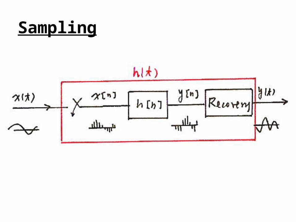
7.0 Sampling 7.1 The Sampling Theorem A link between Continuous-time/Discrete-time Systems x(t) y(t) h(t) x[n] y[n] h[n] Sampling x[n]=x(nT), T : sampling period

7.0 Sampling 7.1 The Sampling Theorem
Dec 31, 2015
7.0 Sampling 7.1 The Sampling Theorem. A link between Continuous-time/Discrete-time Systems. Sampling. x [ n ]. y [ n ]. x ( t ). y ( t ). h [ n ]. h ( t ). x [ n ]= x ( nT ), T : sampling period. Sampling. Motivation: handling continuous-time signals/systems - PowerPoint PPT Presentation
Welcome message from author
This document is posted to help you gain knowledge. Please leave a comment to let me know what you think about it! Share it to your friends and learn new things together.
Transcript

7.0 Sampling
7.1 The Sampling Theorem
A link between Continuous-time/Discrete-time Systems
x(t) y(t)
h(t)
x[n] y[n]
h[n]
Sampling
x[n]=x(nT), T : sampling period
Sampling

Motivation: handling continuous-time signals/systems digitally using computing environment
– accurate, programmable, flexible, reproducible, powerful– compatible to digital networks and relevant technologies– all signals look the same when digitized, except at different rates, thus can be supported by a single network
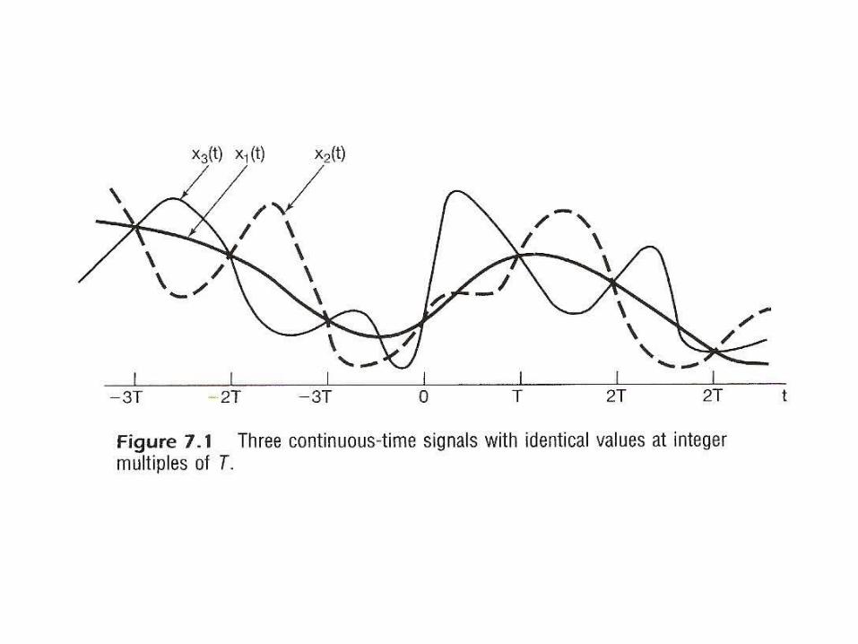
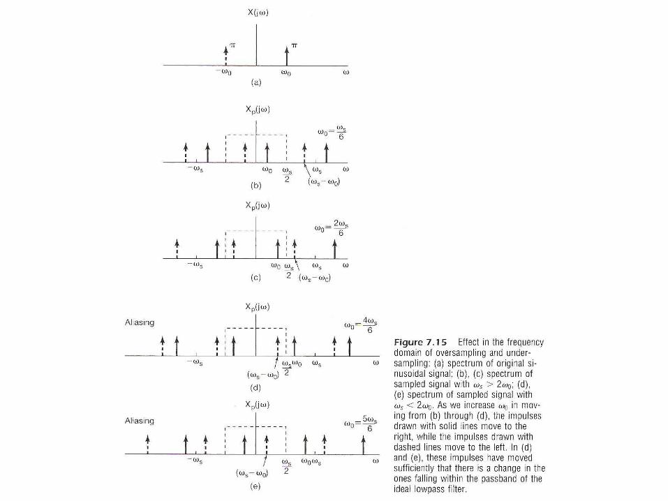
Question: under what kind of conditions can a continuous-time signal be uniquely specified by its discrete-time samples? See Fig. 7.1, p.515 of text
– Sampling Theorem
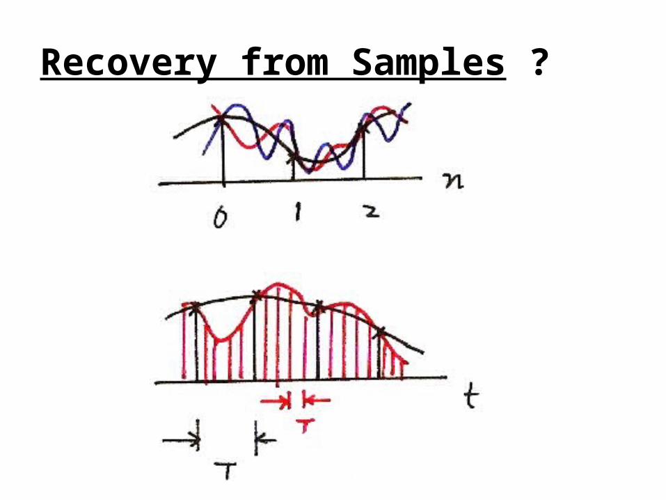
Recovery from Samples ?
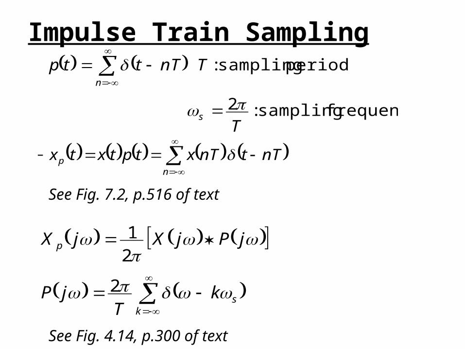
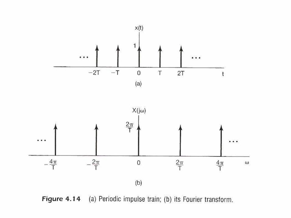
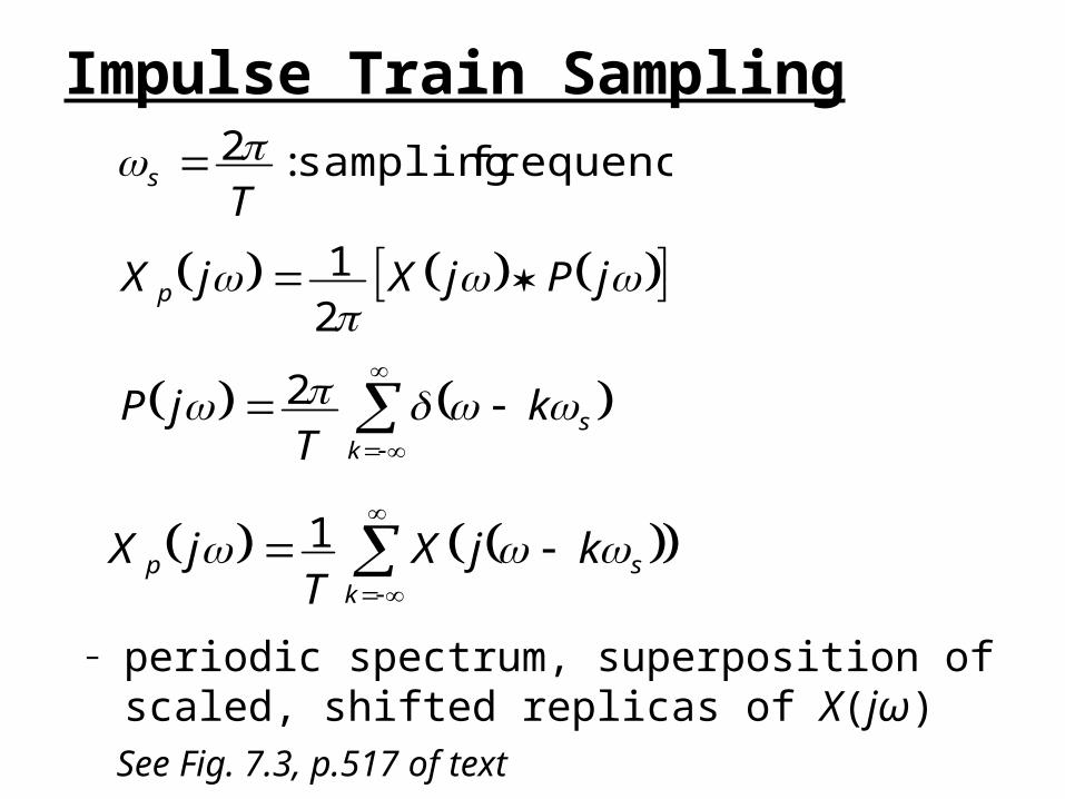
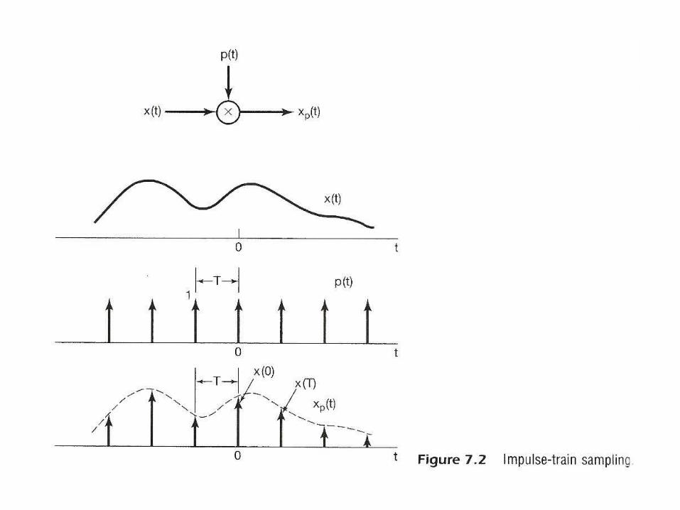
Impulse Train Sampling
frequency sampling : 2
period sampling :
T
TnTttp
s
n
ks
p
kT
jP
jPjXjX
2
21
See Fig. 7.2, p.516 of text
See Fig. 4.14, p.300 of text
nTtnTxtptxtxn
p
–

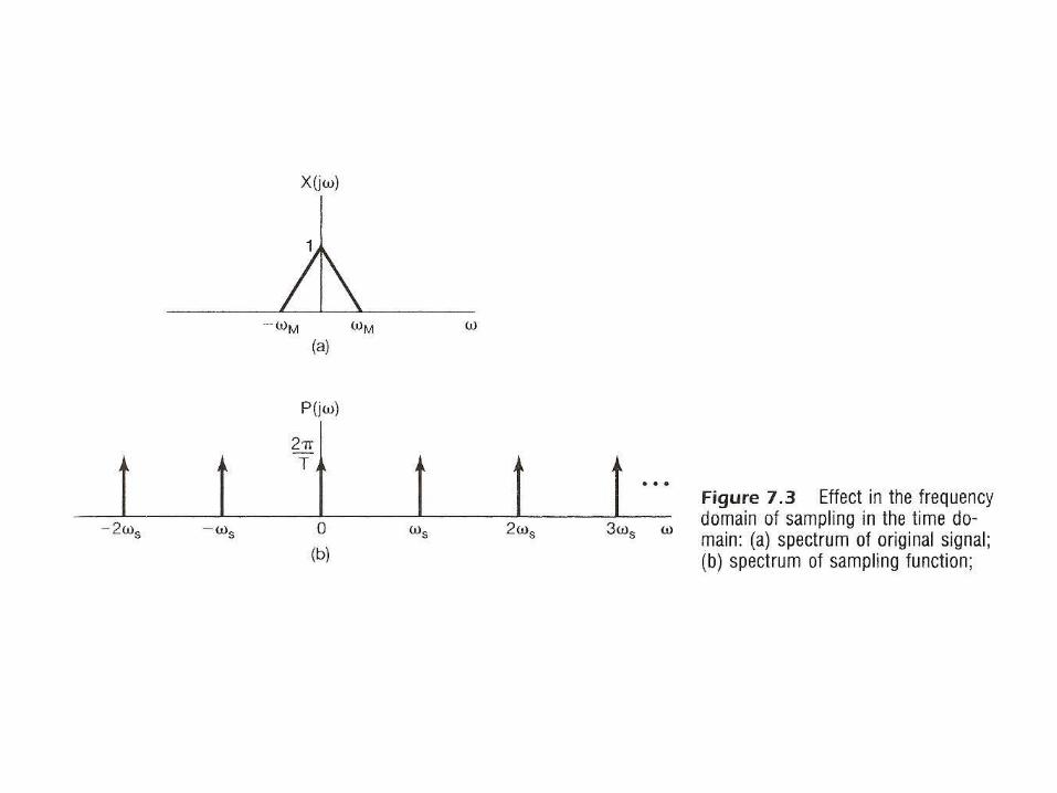
Impulse Train Sampling
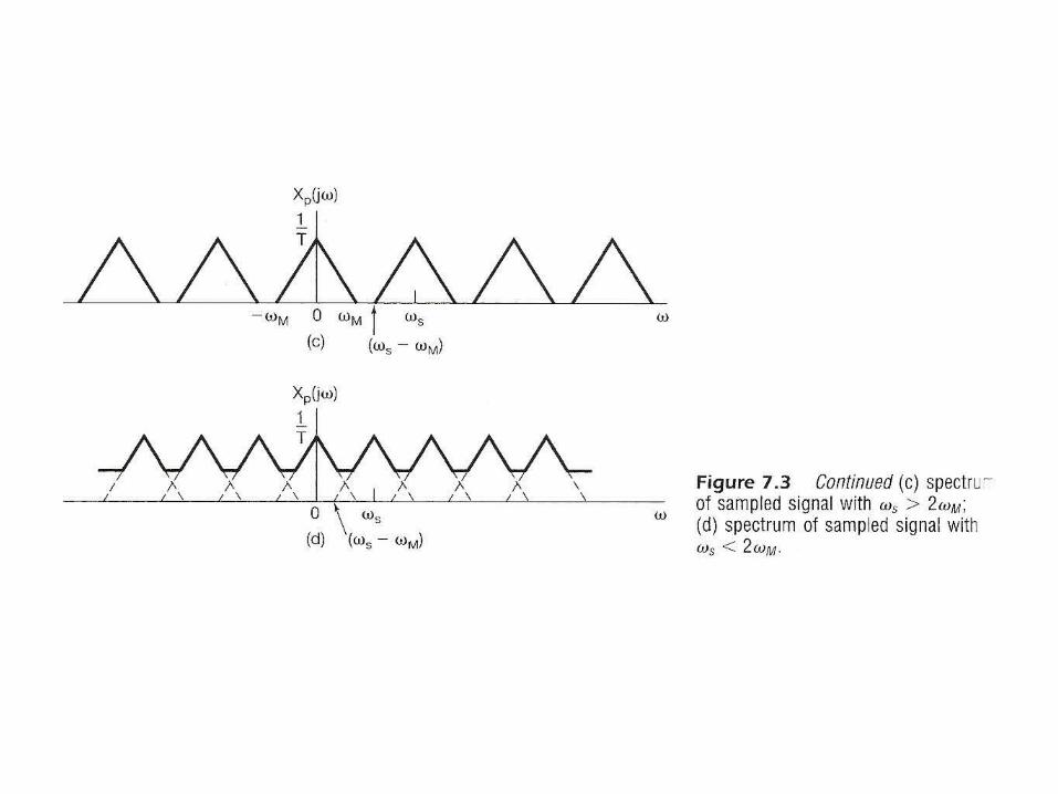
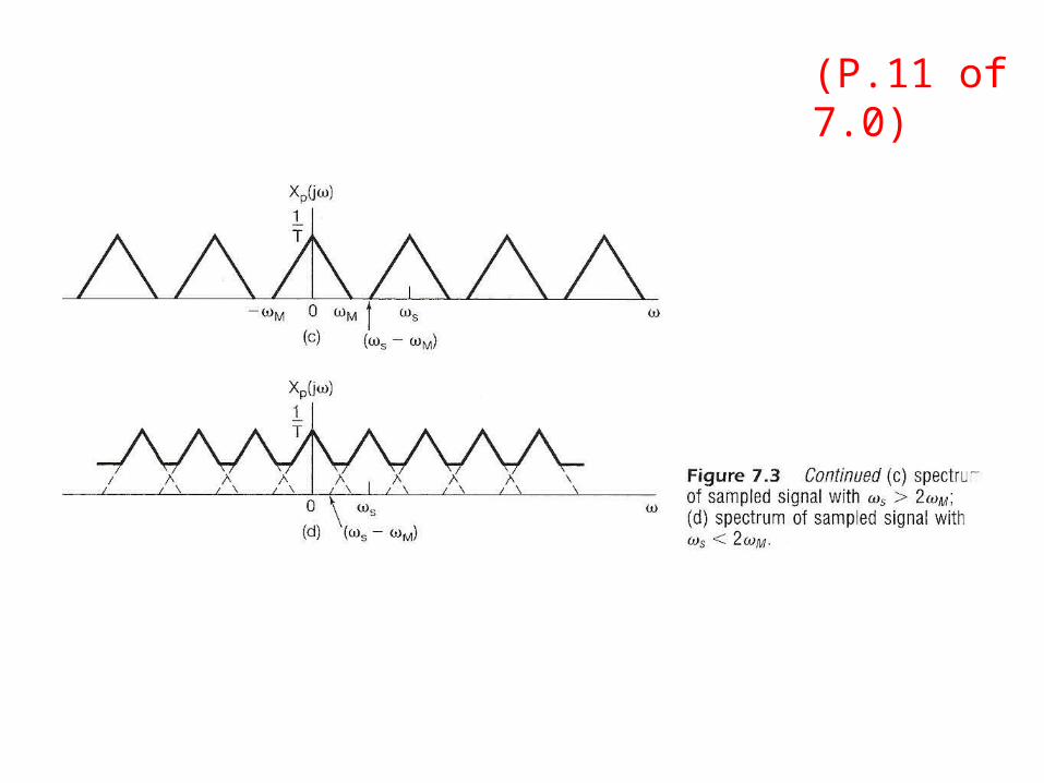
– periodic spectrum, superposition of scaled, shifted replicas of X(jω) See Fig. 7.3, p.517 of text
k
sp kjXT
jX 1
ks
p
s
kT
jP
jPjXjX
T
2
21
frequency sampling : 2

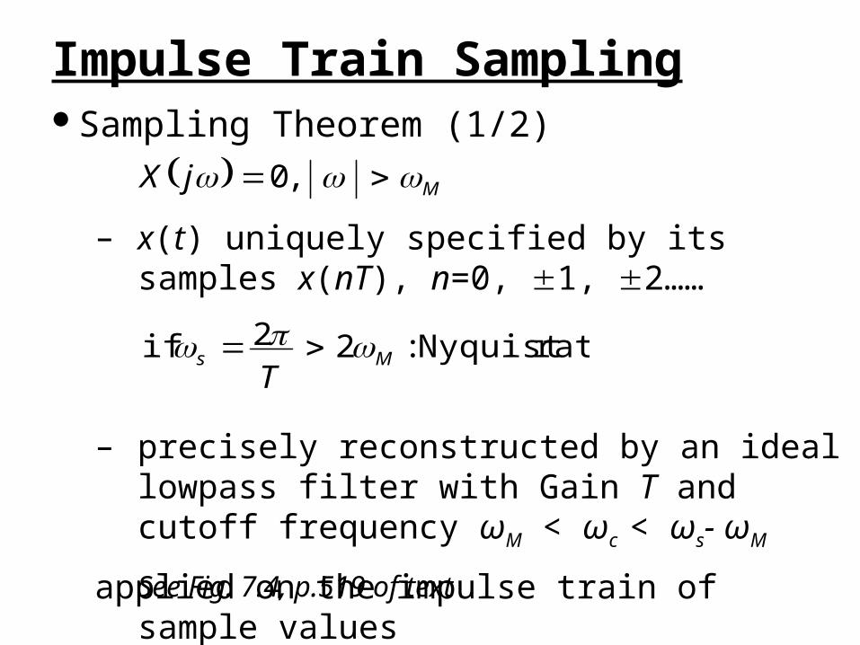
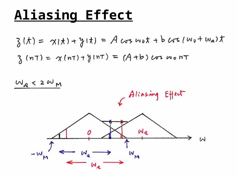
Sampling Theorem (1/2)
MjX ,0
– x(t) uniquely specified by its samples x(nT), n=0, 1, 2……
– precisely reconstructed by an ideal lowpass filter with Gain T and cutoff frequency ωM < ωc < ωs- ωM
applied on the impulse train of sample values
Impulse Train Sampling
rateNyquist : 22 if MsT
See Fig. 7.4, p.519 of text


Sampling Theorem (2/2)
MjX ,0
– if ωs ≤ 2 ωM
spectrum overlapped, frequency components confused --- aliasing effect
can’t be reconstructed by lowpass filtering
Impulse Train Sampling
See Fig. 7.3, p.518 of text
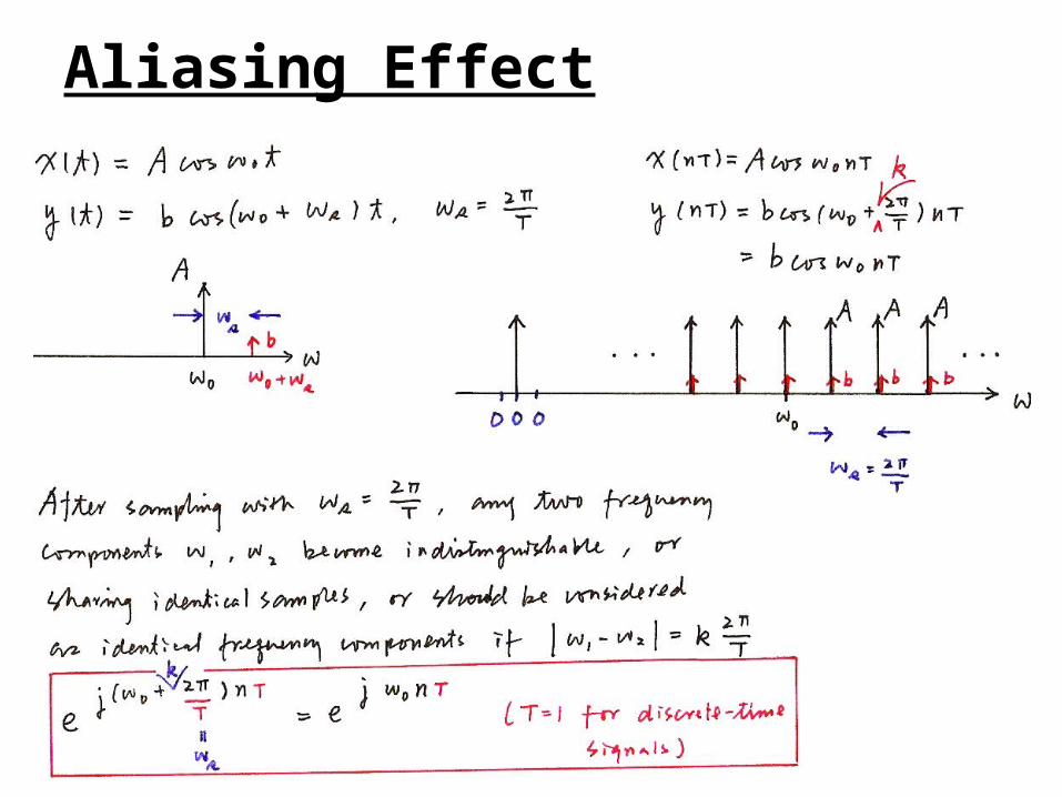
Aliasing Effect
Continuous/Discrete Sinusoidals (p.35 of 1.0)

Sampling
Aliasing Effect

Sampling Thm
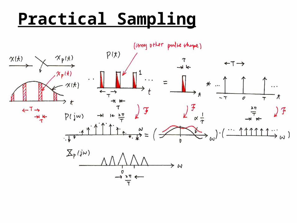
Practical Sampling
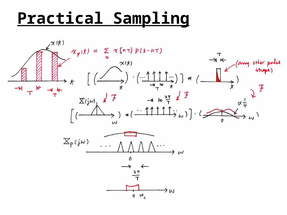
Practical Sampling
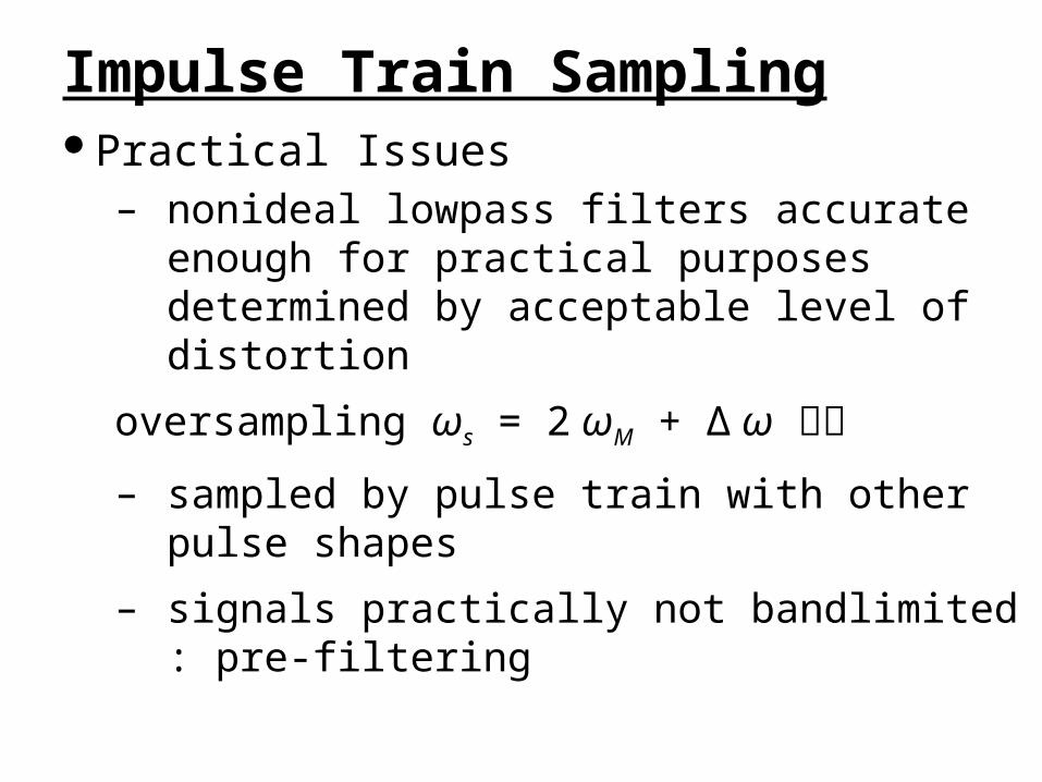
Practical Issues– nonideal lowpass filters accurate enough for
practical purposes determined by acceptable level of distortion
oversampling ωs = 2 ωM + ∆ ω
– sampled by pulse train with other pulse shapes
– signals practically not bandlimited : pre-filtering
Impulse Train Sampling
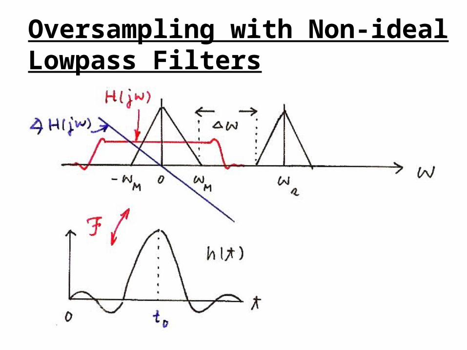
Oversampling with Non-ideal Lowpass Filters

Signals not Bandlimited
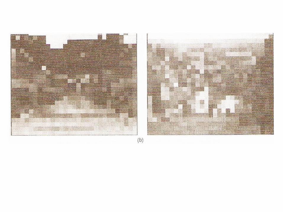
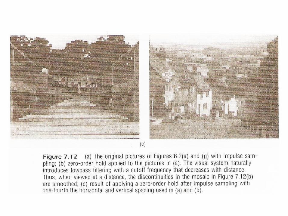
Zero-order Hold:– holding the sampled value until the next sample
taken
– modeled by an impulse train sampler followed by a system with rectangular impulse response
Sampling with A Zero-order Hold
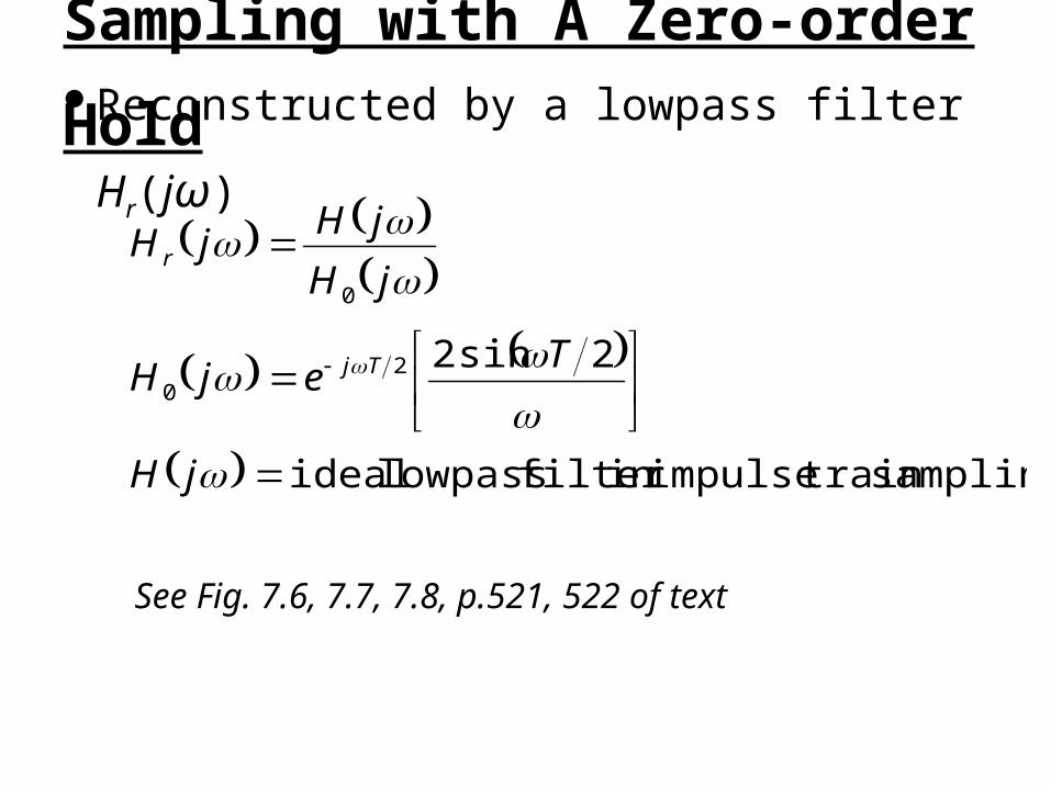
See Fig. 7.6, 7.7, 7.8, p.521, 522 of text
Reconstructed by a lowpass filter Hr(jω)
Sampling with A Zero-order Hold
sampling train impulsein filter lowpass ideal
2sin220
0
jH
TejH
jH
jHjH
Tj
r


Impulse train sampling/ideal lowpass filtering
Interpolation
nTt
nTtTnTxtx
t
tTth
nTthnTxthtxtx
c
cc
nr
c
cc
np
sin
sin
See Fig. 7.10, p.524 of text


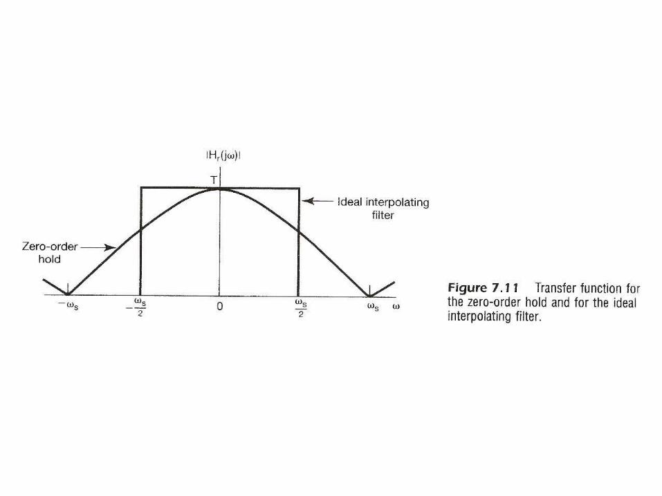
Ideal Interpolation
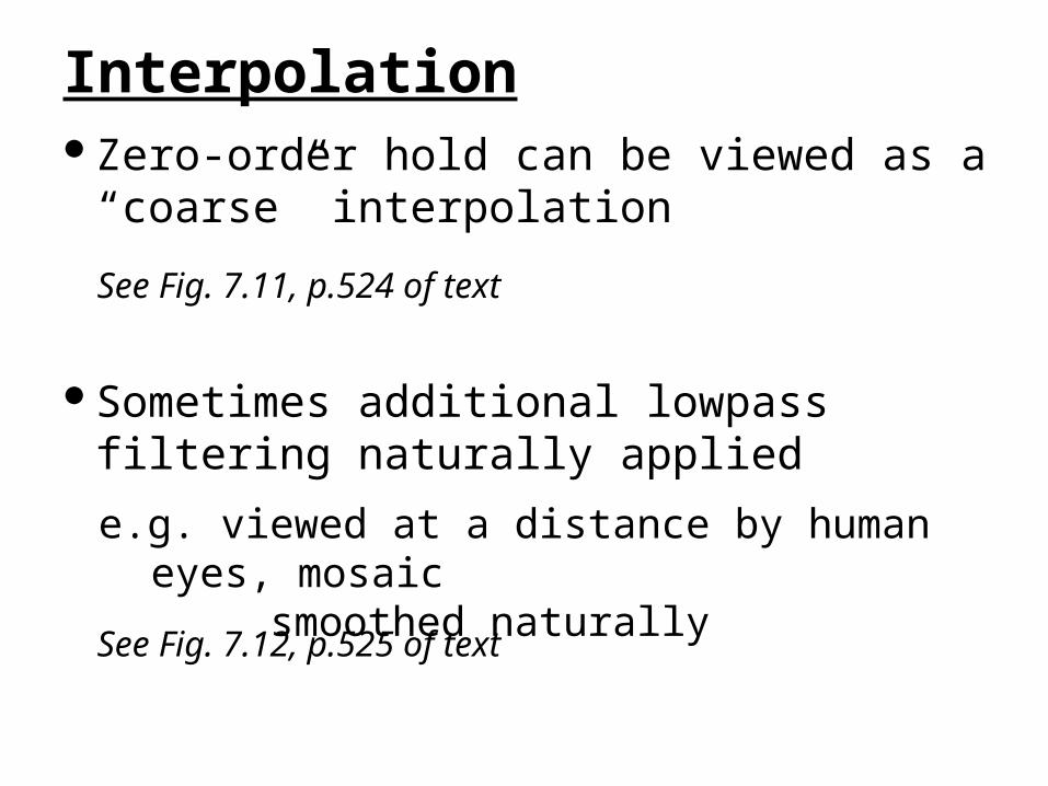
Zero-order hold can be viewed as a “coarse” interpolation
Interpolation
See Fig. 7.12, p.525 of text
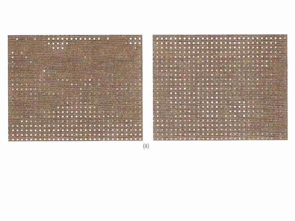
Sometimes additional lowpass filtering naturally applied
See Fig. 7.11, p.524 of text
e.g. viewed at a distance by human eyes, mosaic smoothed naturally
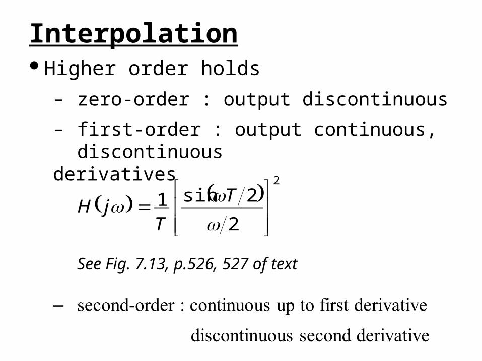
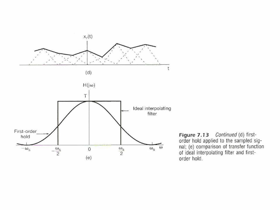
Higher order holds
Interpolation
See Fig. 7.13, p.526, 527 of text
– zero-order : output discontinuous
– first-order : output continuous, discontinuous derivatives
2
2
2sin1
T
TjH


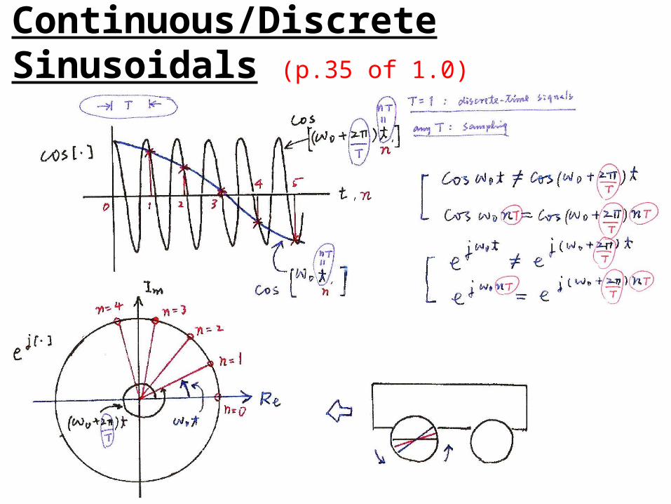
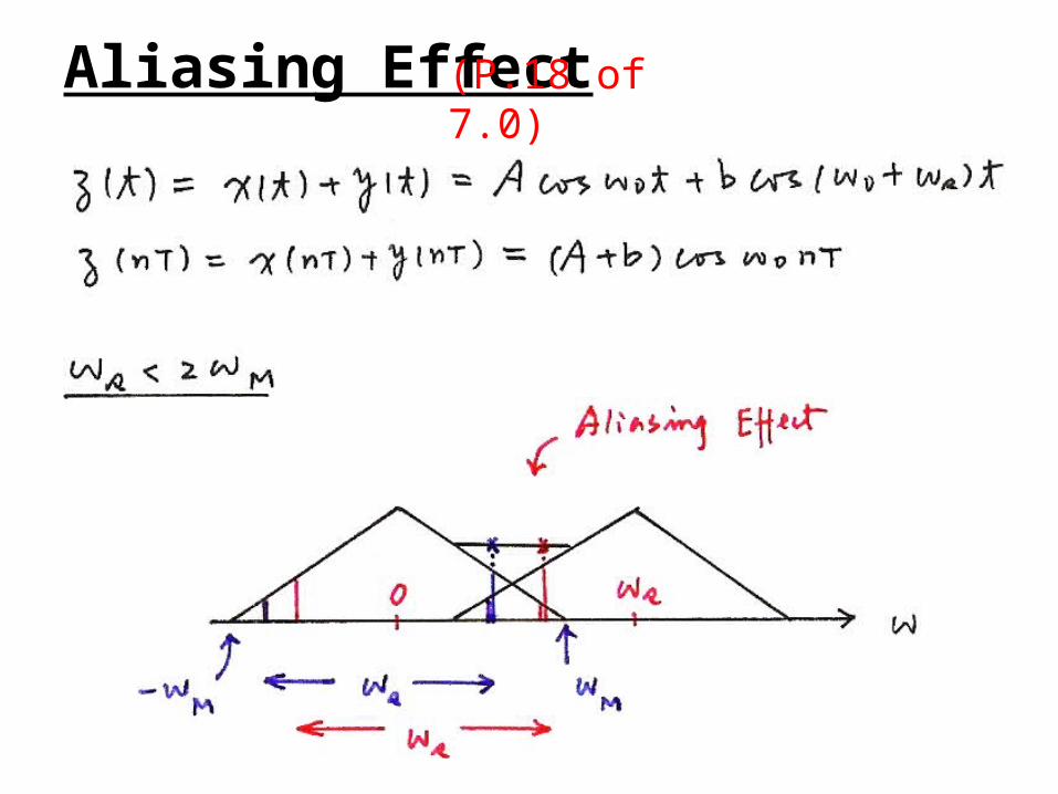
Consider a signal x(t)=cos ω0t
Aliasing
– sampled at sampling frequency
reconstructed by an ideal lowpass filter
with
xr(t) : reconstructed signal
fixed ωs, varying ω0
Ts
2
2s
c
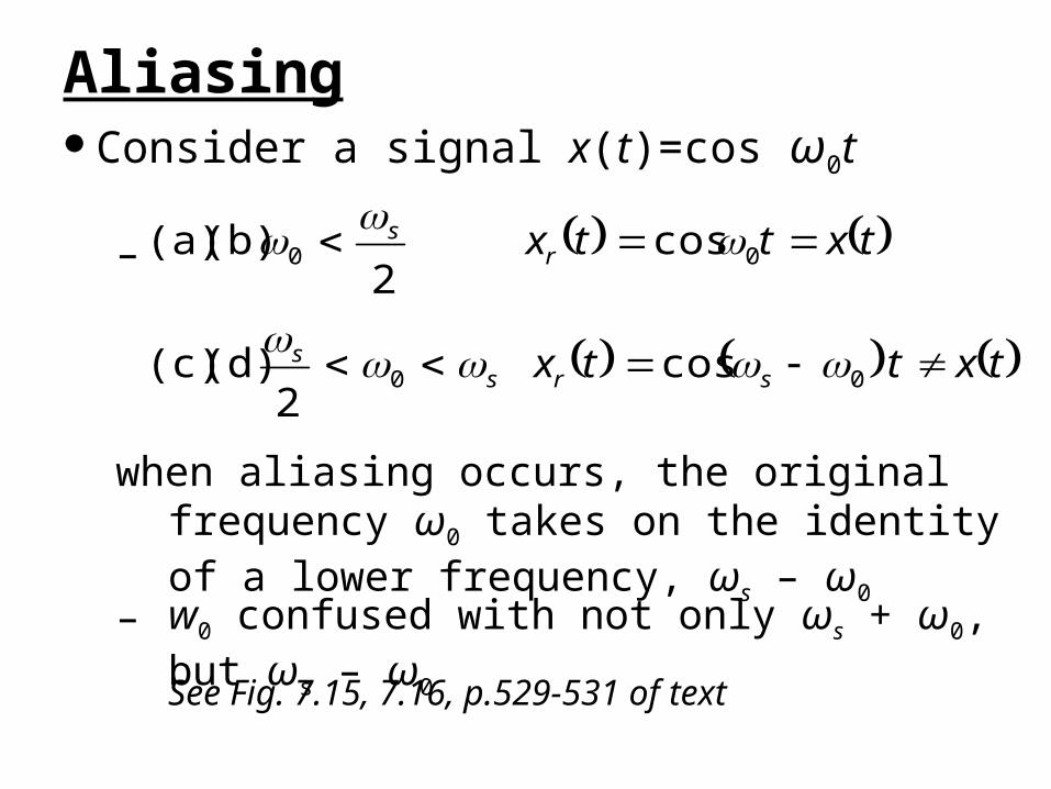
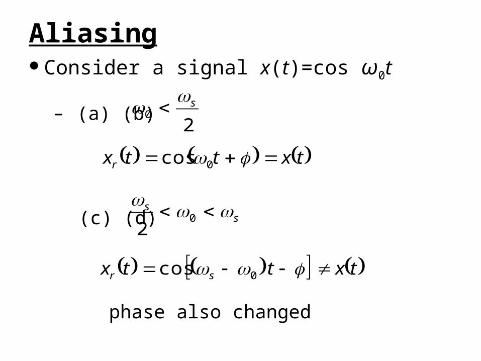
Consider a signal x(t)=cos ω0t
Aliasing
–
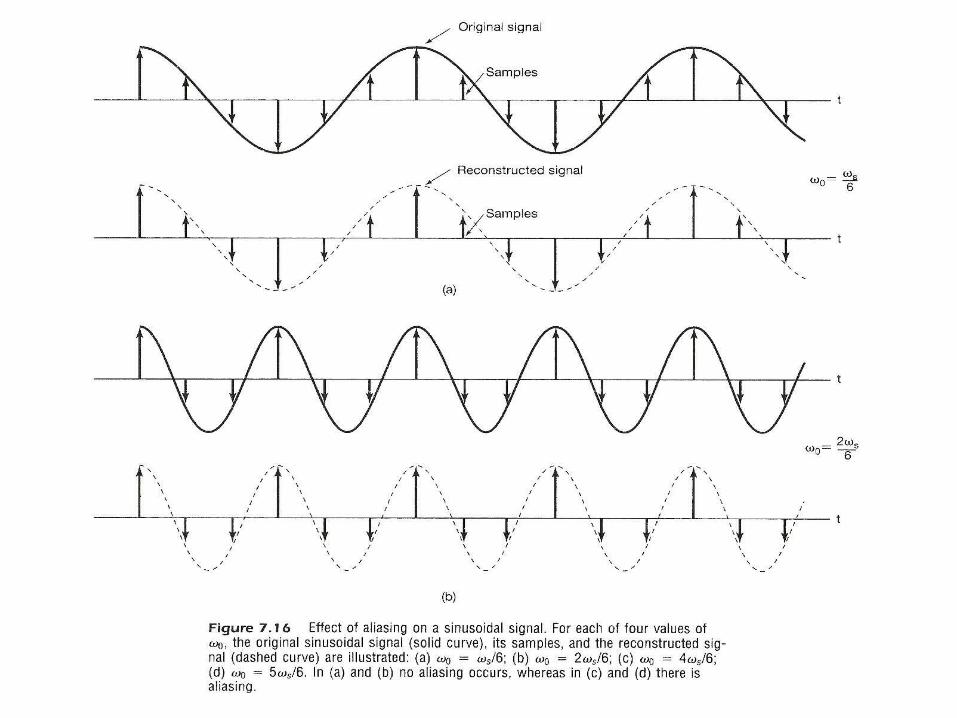
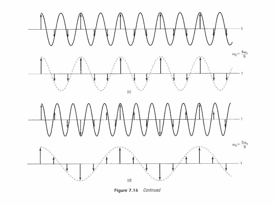
when aliasing occurs, the original frequency ω0 takes on the identity of a lower frequency, ωs – ω0
txttx
txttx
srss
rs
cos 2
(d) (c)
cos 2
(b) (a)
00
00
See Fig. 7.15, 7.16, p.529-531 of text
– w0 confused with not only ωs + ω0, but ωs – ω0
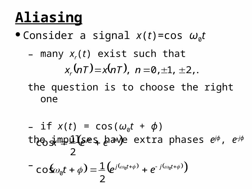
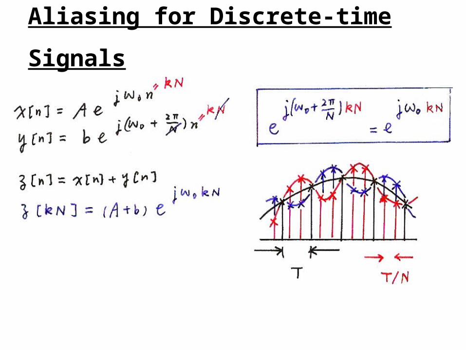
Consider a signal x(t)=cos ω0t
Aliasing
– many xr(t) exist such that
the question is to choose the right one
– if x(t) = cos(ω0t + ϕ)the impulses have extra phases ejϕ, e-jϕ
–
... ,2 ,1 ,0 , nnTxnTxr
tjtj
jxjx
eet
eex
00
21cos
21cos
0
Sinusoidals (p.64 of 4.0)
Consider a signal x(t)=cos ω0t
Aliasing
– (a) (b)2
0s
txttxr 0cos
ss
02
(c) (d)
txttx sr cos 0
phase also changed
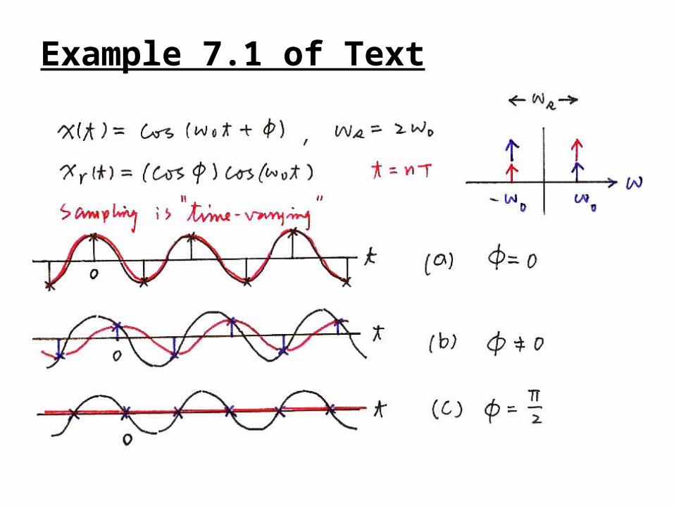
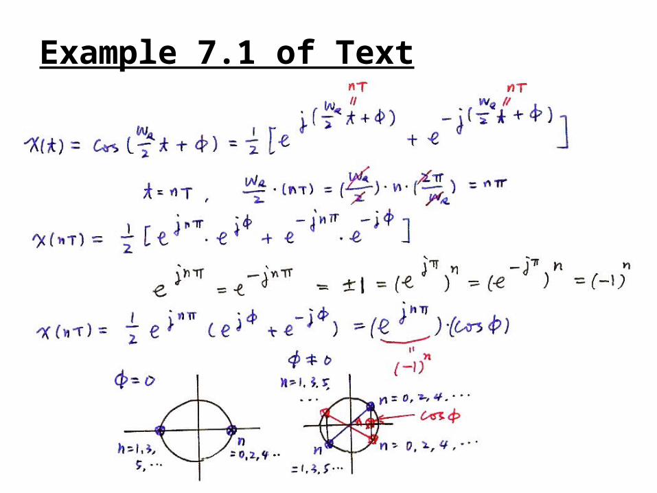
Example 7.1 of Text
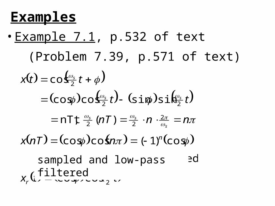
Examples• Example 7.1, p.532 of text
(Problem 7.39, p.571 of text)
ttx
nnTx
nnnT
tt
ttx
s
s
ss
ss
s
r
n
2
222
22
2
coscos
filtered pass-low and sampled
cos)1(coscos
)( nT, t
sinsincoscos
cos
sampled and low-pass filtered

Example 7.1 of Text
Example 7.1 of Text
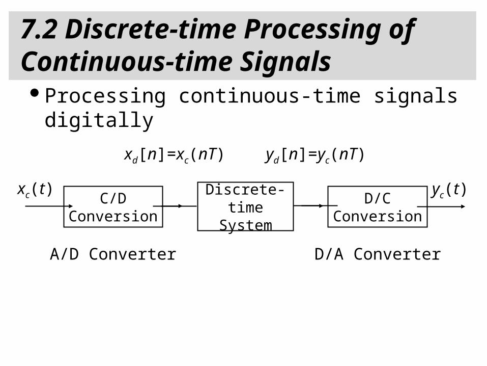
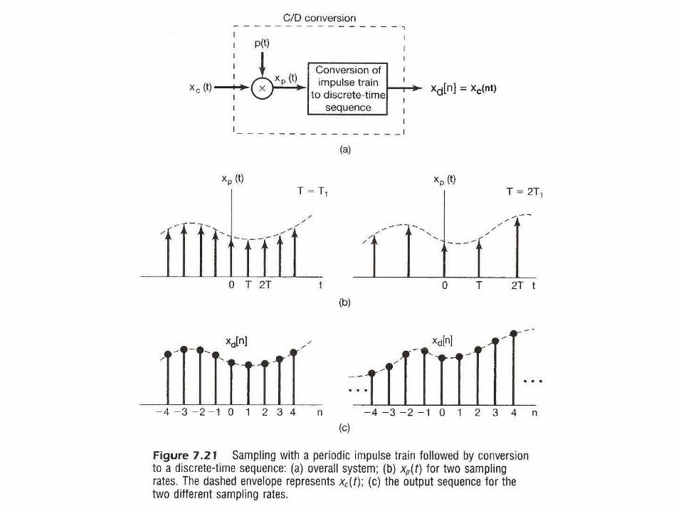
7.2 Discrete-time Processing of Continuous-time Signals
Processing continuous-time signals digitally
C/DConversion
xc(t) yc(t)
A/D Converter
D/CConversion
D/A Converter
Discrete-timeSystem
xd[n]=xc(nT) yd[n]=yc(nT)

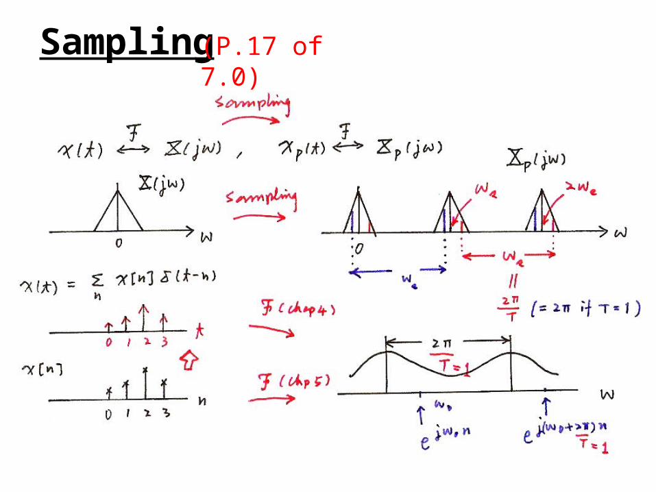
Sampling (p.2 of 7.0)
C/D Conversion
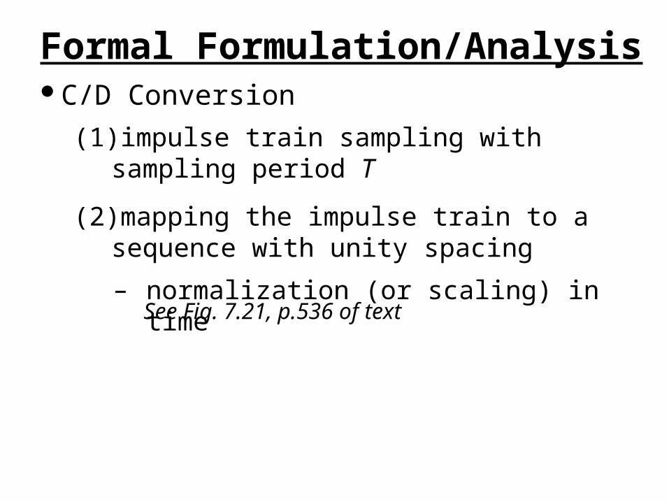
Formal Formulation/Analysis
(1) impulse train sampling with sampling period T
(2) mapping the impulse train to a sequence with unity spacing
– normalization (or scaling) in time
See Fig. 7.21, p.536 of text
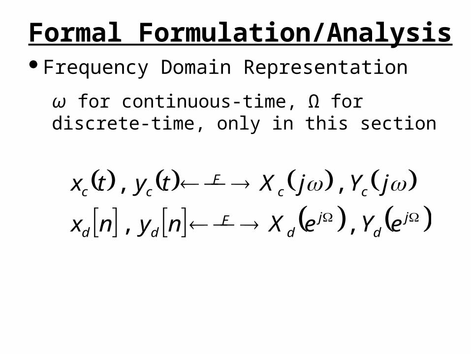
Frequency Domain Representation
Formal Formulation/Analysis
ω for continuous-time, Ω for discrete-time, only in this section
j
dj
dF
dd
ccF
cc
eYeXnynx
jYjXtytx
, ,
, ,

Frequency Domain Relationships
Formal Formulation/Analysis
– continuous-time
nTj
kcp
kcp
enTxjX
nTtnTxtx
nj
kc
jd
cd
enTxeX
nTxnx
– discrete-time
C/D Conversion
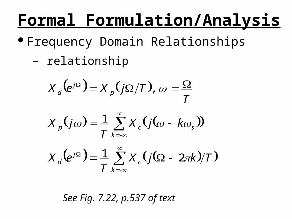
Frequency Domain Relationships
Formal Formulation/Analysis
– relationship
TkjXT
eX
kjXT
jX
TTjXeX
kc
jd
sk
cp
pj
d
21
1
,
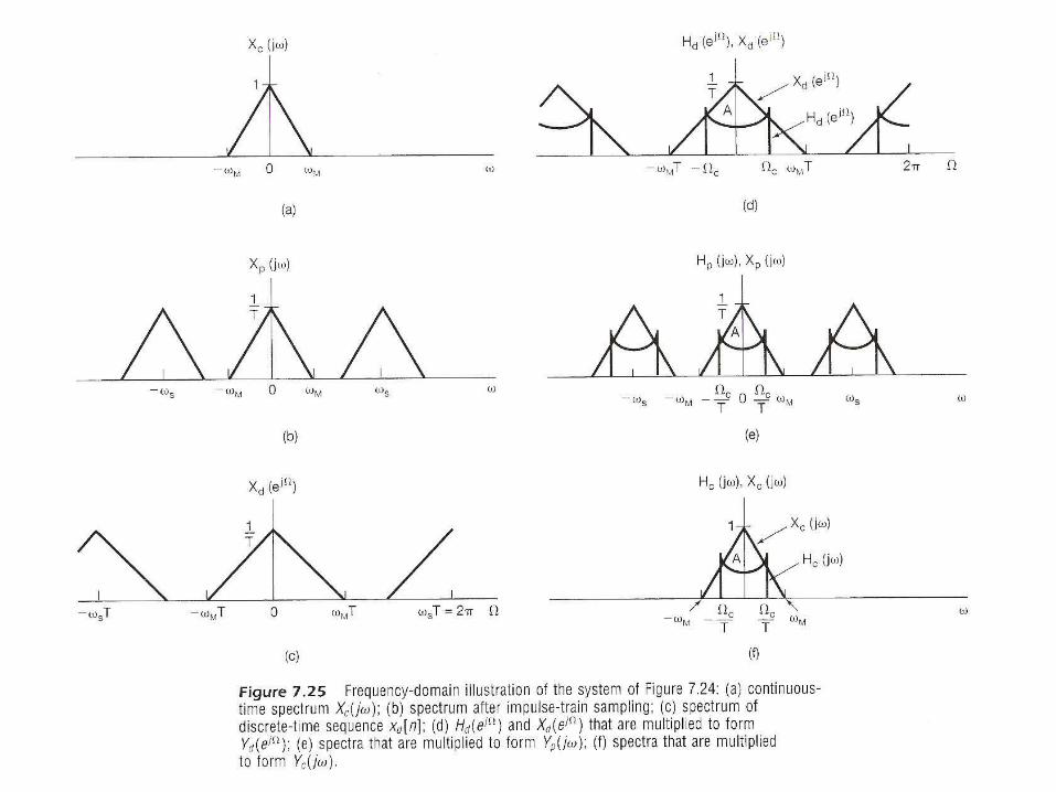
See Fig. 7.22, p.537 of text
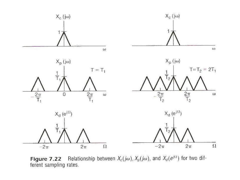
Frequency Domain Relationships
Formal Formulation/Analysis
– Xd(ejΩ) is a frequency-scaled (by T) version of Xp(jω)
xd[n] is a time-scaled (by 1/T) version of xp(t)
– Xd(ejΩ) periodic with period 2π
xd[n] discrete in time
Xp(jω) periodic with period 2π/T=ωs
xp(t) obtained by impulse train sampling

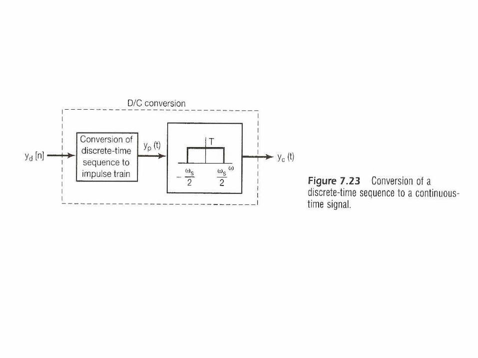
D/C Conversion
Formal Formulation/Analysis
(1) mapping a sequence to an impulse train
(2) lowpass filtering
See Fig. 7.23, p.538 of text

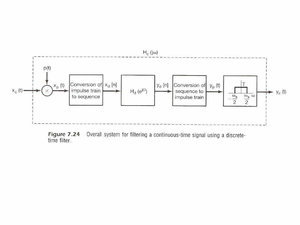
Complete System
Formal Formulation/Analysis
equivalent to a continuous-time system
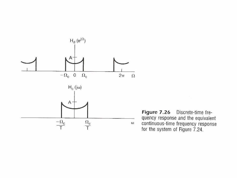
See Fig. 7.24, 7.25, 7.26, p.538, 539, 540 of text
Tjdcc eHjXjY
2 0,
2 ,
s
sTj
dc eHjH
if the sampling theorem is satisfied
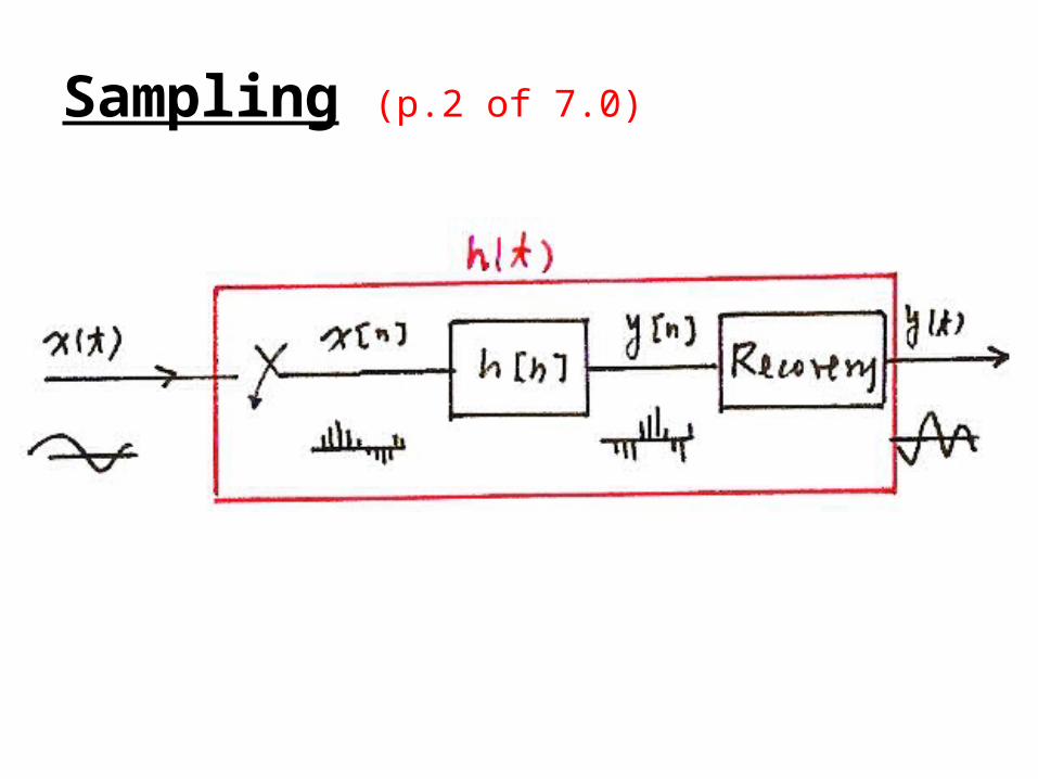
Sampling (p.2 of 7.0)
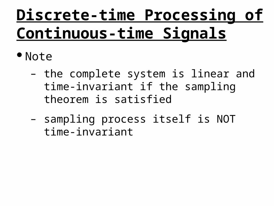
Note
Discrete-time Processing of Continuous-time Signals
– the complete system is linear and time-invariant if the sampling theorem is satisfied
– sampling process itself is NOT time-invariant
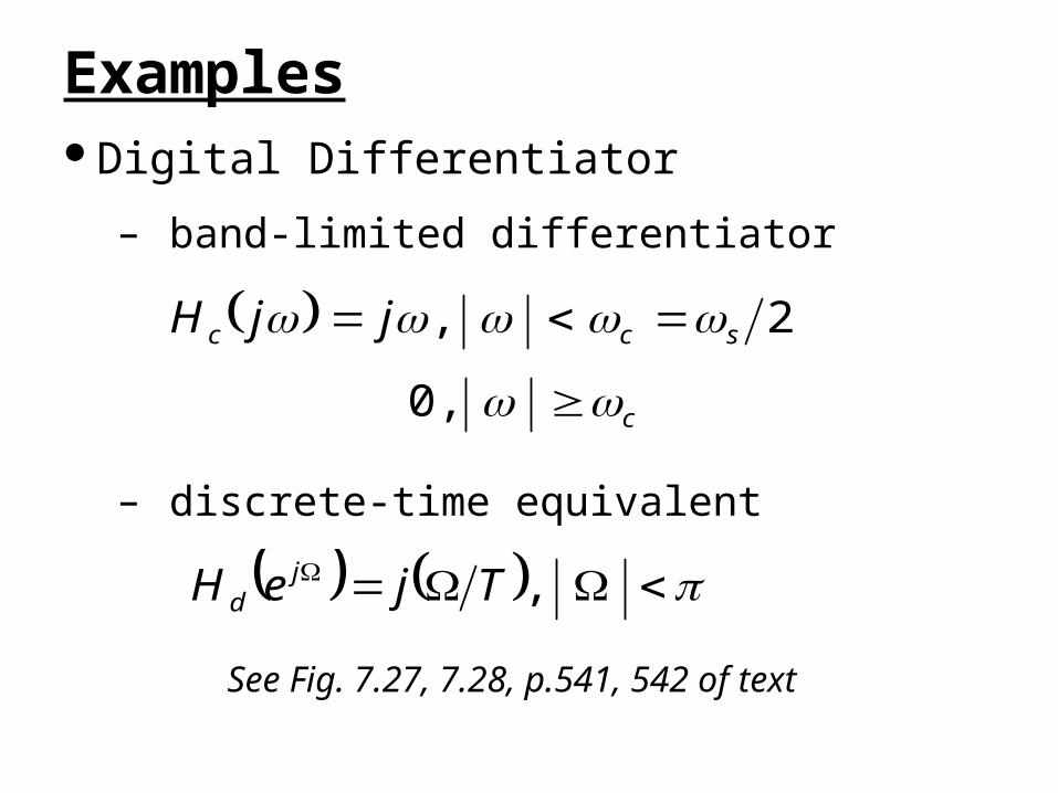
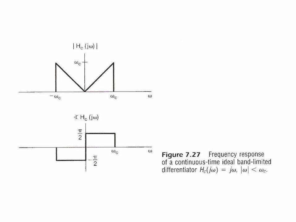
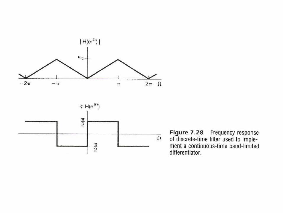
Digital Differentiator
Examples
– band-limited differentiator
– discrete-time equivalent
c
scc jjH
0,
2 ,
,TjeH jd
See Fig. 7.27, 7.28, p.541, 542 of text

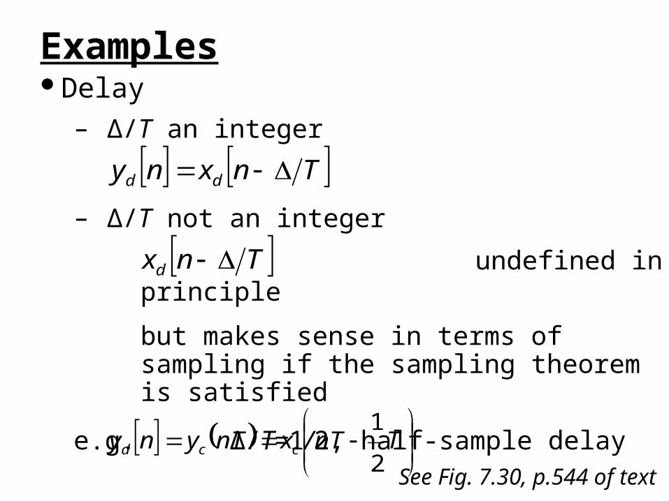
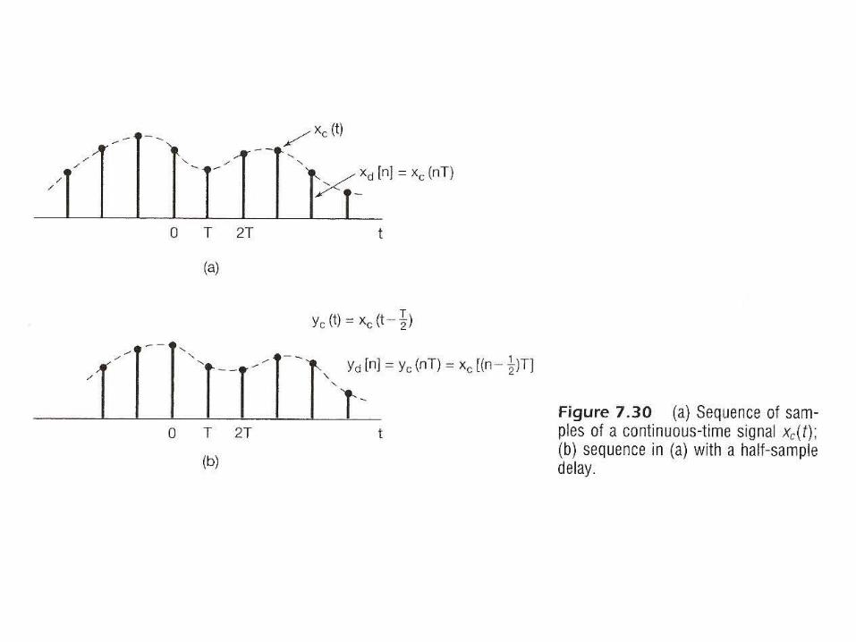
Delay
Examples
– yc(t)=xc(t-∆)
– discrete-time equivalent
c
scj
c ejH
, 0
2 ,
,Tjjd jeH
See Fig. 7.29, p.543 of text

Tnxny dd
Delay
Examples
– ∆/T an integer
– ∆/T not an integer
undefined in principle
but makes sense in terms of sampling if the sampling theorem is satisfied
e.g. ∆/T=1/2, half-sample delay
See Fig. 7.30, p.544 of text
Tnxd
TnTxnTyny ccd
2
1
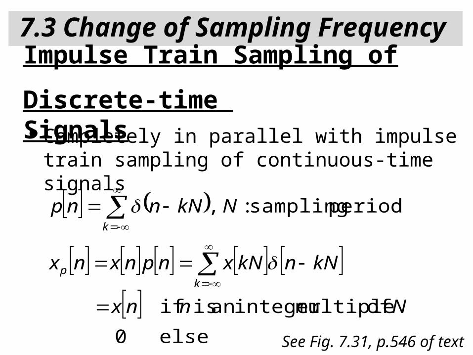
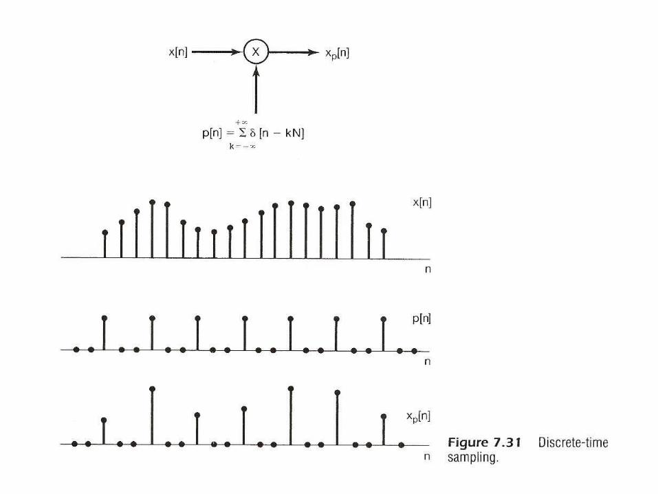
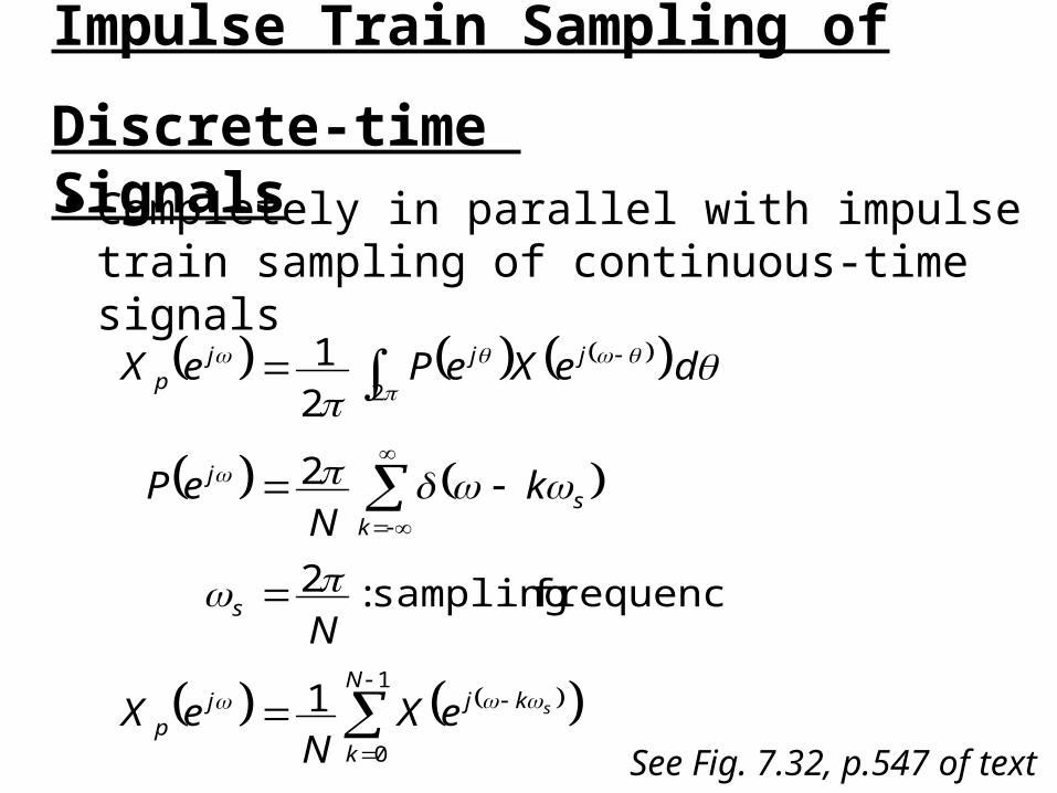
7.3 Change of Sampling Frequency
Completely in parallel with impulse train sampling of continuous-time signals
Impulse Train Sampling of Discrete-time Signals
else 0
of multipleinteger an is if
period sampling : ,
Nnnx
kNnkNxnpnxnx
NkNnnp
kp
k
See Fig. 7.31, p.546 of text
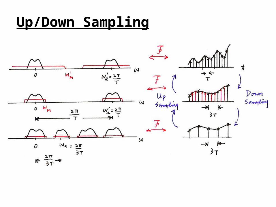
Up/Down Sampling
(P.11 of 7.0)
Completely in parallel with impulse train sampling of continuous-time signals
Impulse Train Sampling of Discrete-time Signals
1
0
2
1
frequency sampling : 2
2
21
N
k
kjjp
s
ks
j
jjjp
seXN
eX
N
kN
eP
deXePeX
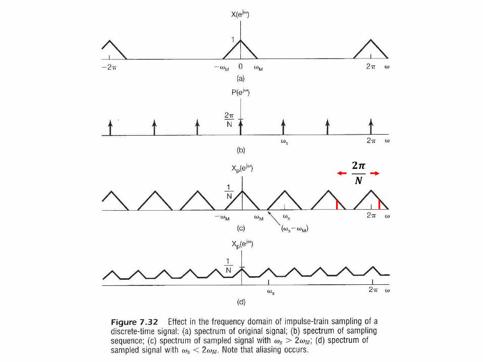
See Fig. 7.32, p.547 of text

Aliasing Effect (P.15 of 7.0)
Sampling (P.17 of 7.0)
Aliasing Effect (P.18 of 7.0)
Aliasing for Discrete-time Signals
Completely in parallel with impulse train sampling of continuous-time signals
Impulse Train Sampling of Discrete-time Signals
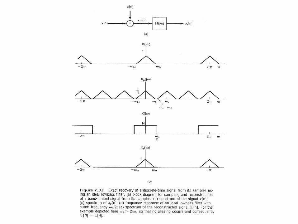
– ωs > 2ωM, no aliasing
x[n] can be exactly recovered from xp[n] by a lowpass filter
With Gain N and cutoff frequency ωM < ωc < ωs- ωMSee Fig. 7.33, p.548 of text
– ωs > 2ωM, aliasing occurs
filter output xr[n] ≠ x[n]
but xr[kN] = x[kN], k=0, ±1, ±2, ……
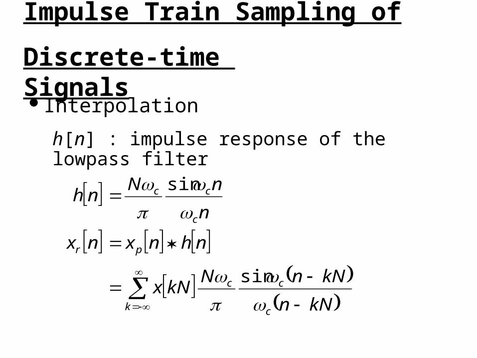
Interpolation
Impulse Train Sampling of Discrete-time Signals
h[n] : impulse response of the lowpass filter
kNn
kNnNkNx
nhnxnx
n
nNnh
c
cc
k
pr
c
cc
sin
sin


Interpolation
Impulse Train Sampling of Discrete-time Signals
– in general a practical filter hr[n] is used
kNnhkNx
nhnxnx
kr
rpr
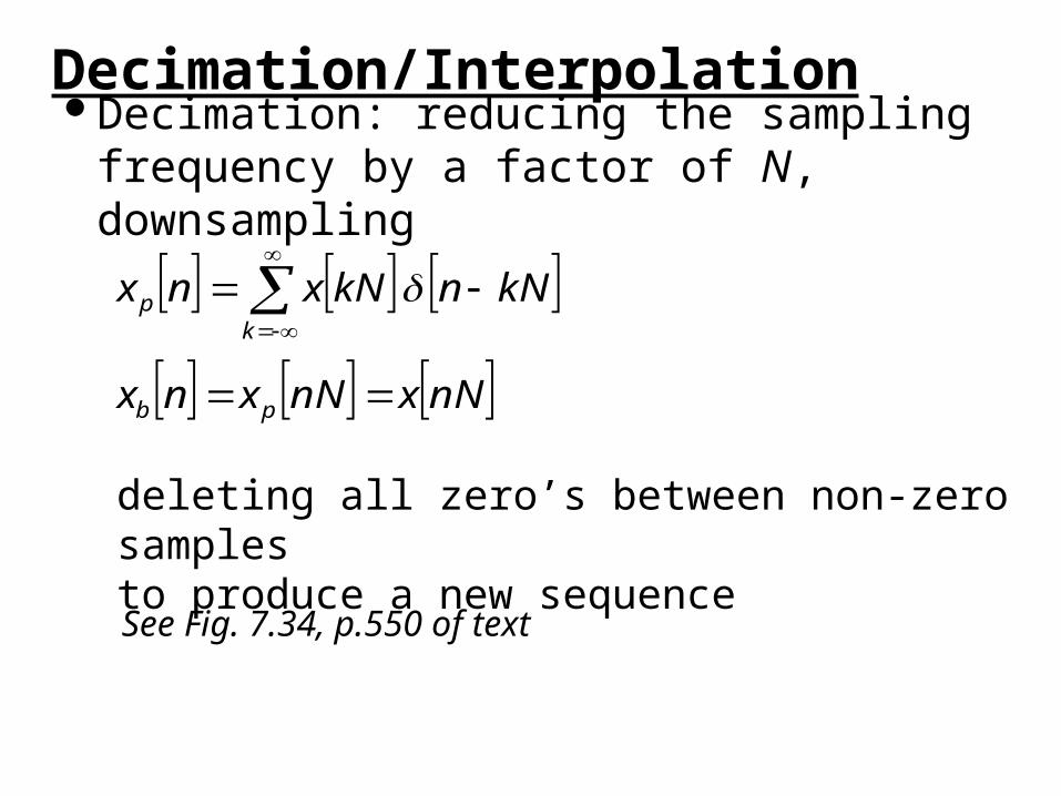
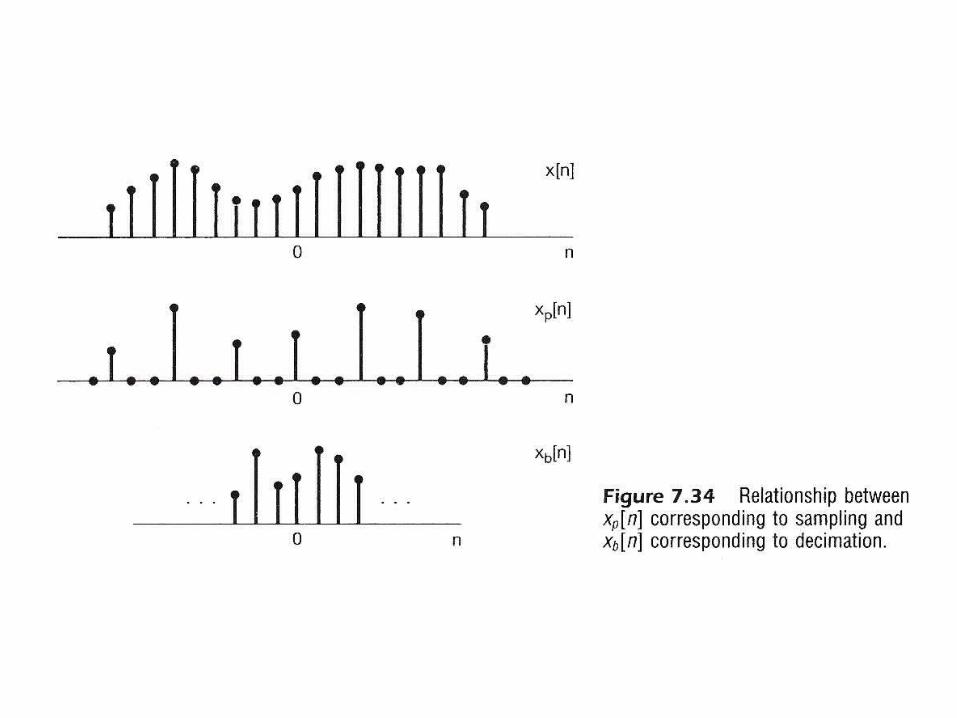
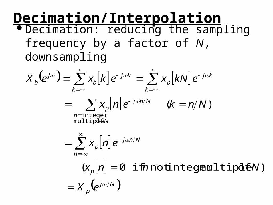
Decimation: reducing the sampling frequency by a factor of N, downsampling
Decimation/Interpolation
deleting all zero’s between non-zero samplesto produce a new sequence
nNxnNxnx
kNnkNxnx
pb
kp
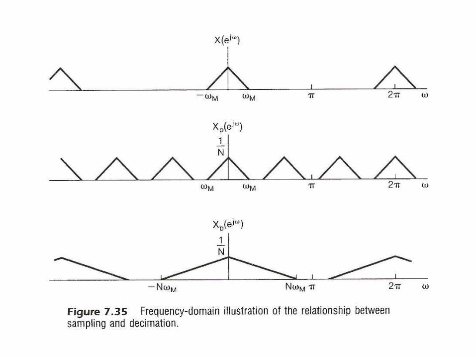
See Fig. 7.34, p.550 of text
jF eXnx
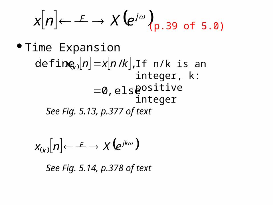
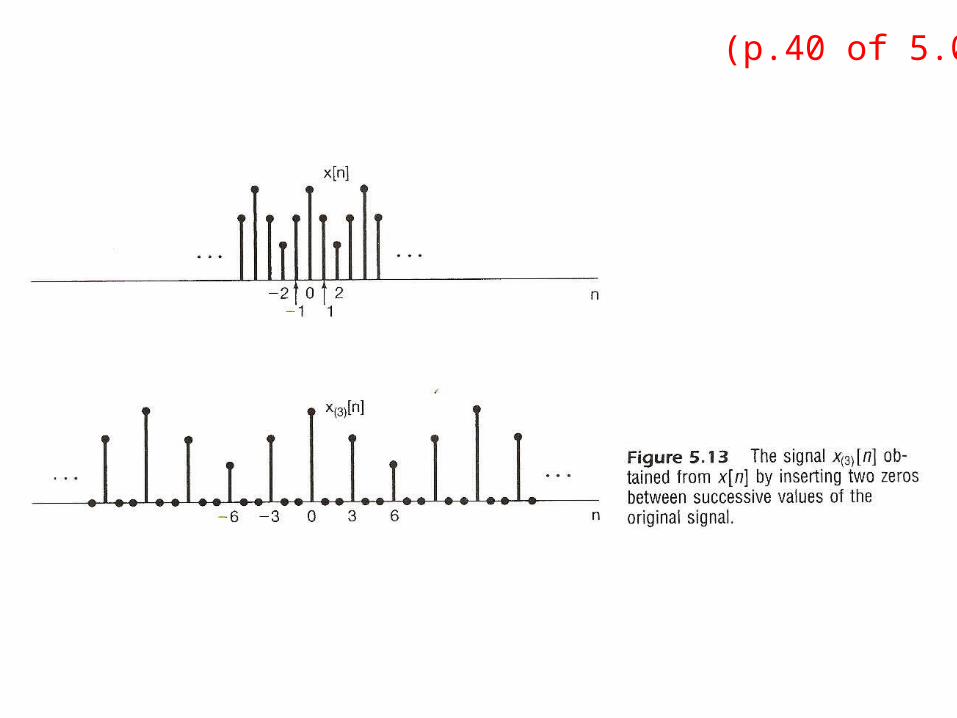
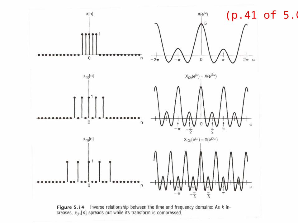
Time Expansion
else ,0
,/ define
knxnx k If n/k is an integer, k: positive integer
See Fig. 5.14, p.378 of text
See Fig. 5.13, p.377 of text
jkFk eXnx
(p.39 of 5.0)
(p.40 of 5.0)
(p.41 of 5.0)
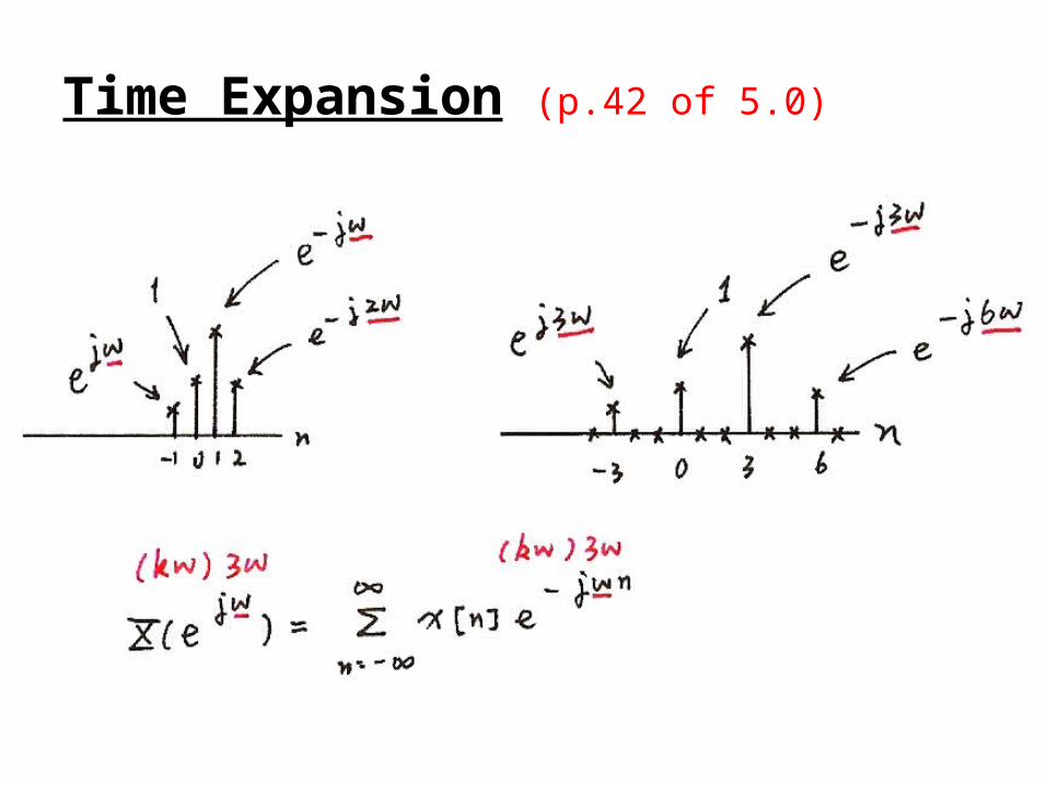
Time Expansion (p.42 of 5.0)
Decimation: reducing the sampling frequency by a factor of N, downsampling
Decimation/Interpolation
Nj
p
p
Nnj
-np
Nn
Nnjp
k
kjp
k
kjb
jb
eX
Nnnx
enx
Nnkenx
ekNxekxeX
) of multipleinteger not if 0(
)(
of multipleinteger

Decimation
Decimation/Interpolation
– Scaled in frequency
inverse of time expansion property of discrete-time Fourier transform
See Fig. 7.35, p. 551 of text
– decimation without introducing aliasing requires oversampling situation
See an example in Fig. 7.36, p. 552 of text

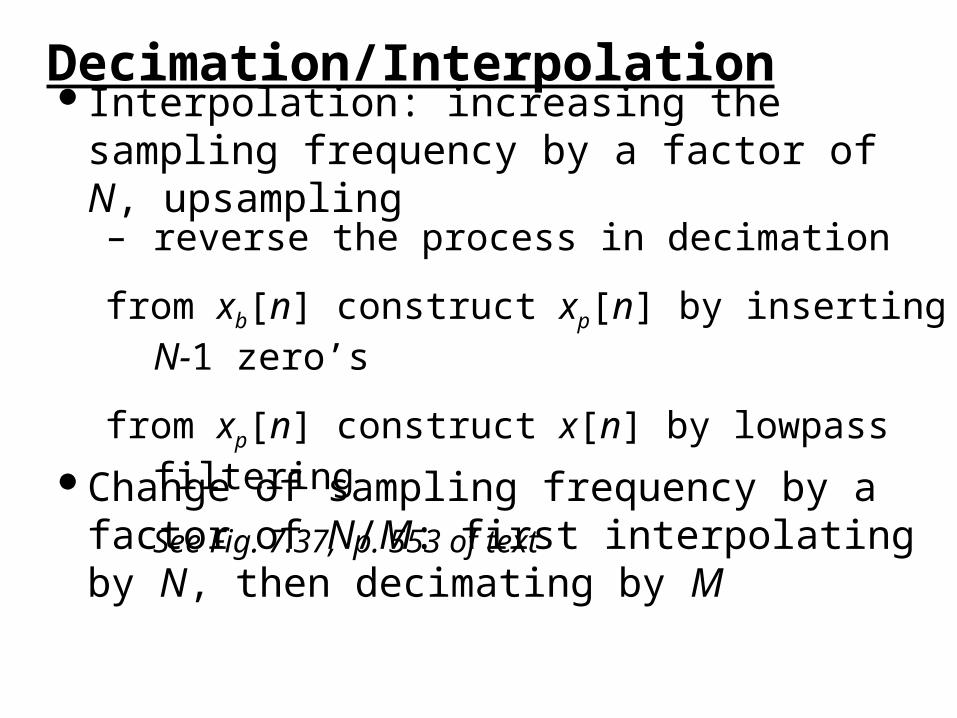
Interpolation: increasing the sampling frequency by a factor of N, upsampling
Decimation/Interpolation
– reverse the process in decimation
from xb[n] construct xp[n] by inserting N-1 zero’s
from xp[n] construct x[n] by lowpass filtering
See Fig. 7.37, p. 553 of text
Change of sampling frequency by a factor of N/M: first interpolating by N, then decimating by M

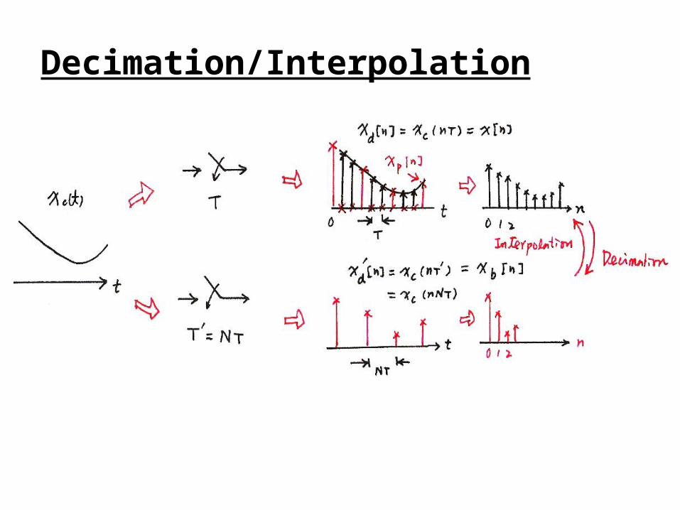
Decimation/Interpolation
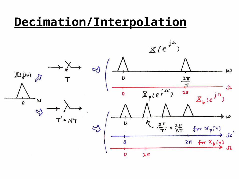
Decimation/Interpolation

Examples• Example 7.4/7.5, p.548, p.554 of text
sampling x[n] without aliasing
9
2for 0 , jj eXeXnx
2422 ,4
29N , 9
2222
maxmax
NN
N
s
Ms
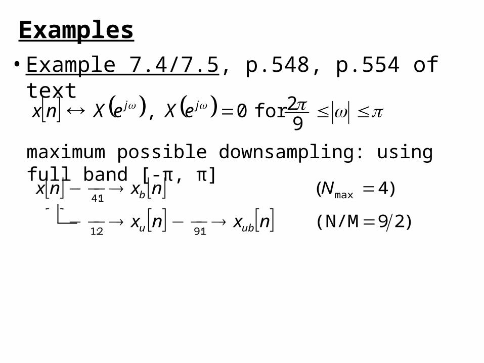
Examples• Example 7.4/7.5, p.548, p.554 of text
maximum possible downsampling: using full band [-π, π]
9
2for 0 , jj eXeXnx
)29(N/M
)4(
1:92:1
max1:4
nxnxnx
Nnxnx
ubu
b

Examples• Example 7.4/7.5, p.548, p.554 of text
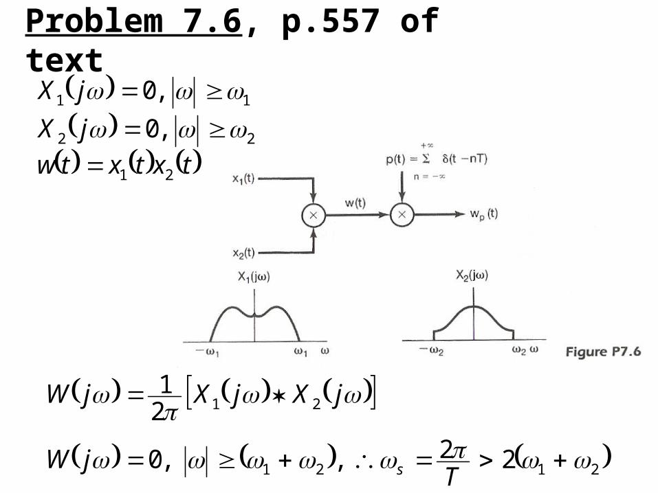
Problem 7.6, p.557 of text
txtxtw
jX
jX
21
22
11
,0
,0
2121
21
22 , ,0
21
TjW
jXjXjW
s
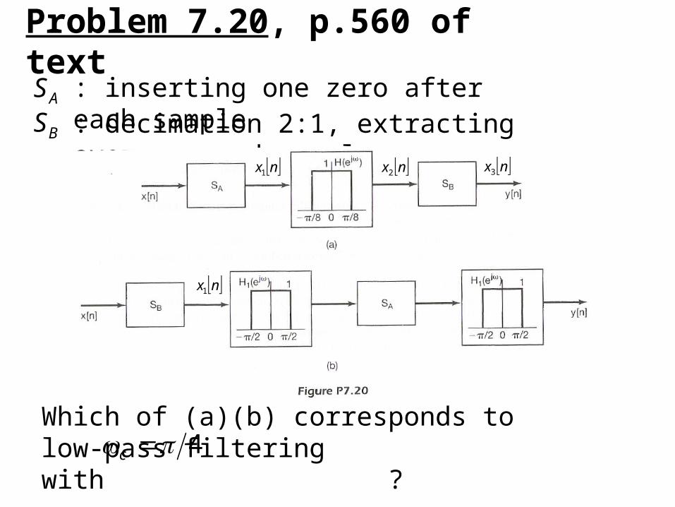
Problem 7.20, p.560 of text
B
A
SS : inserting one zero after each sample
: decimation 2:1, extracting every second sample
Which of (a)(b) corresponds to low-pass filteringwith ?4 c
nx1 nx2 nx3
nx1
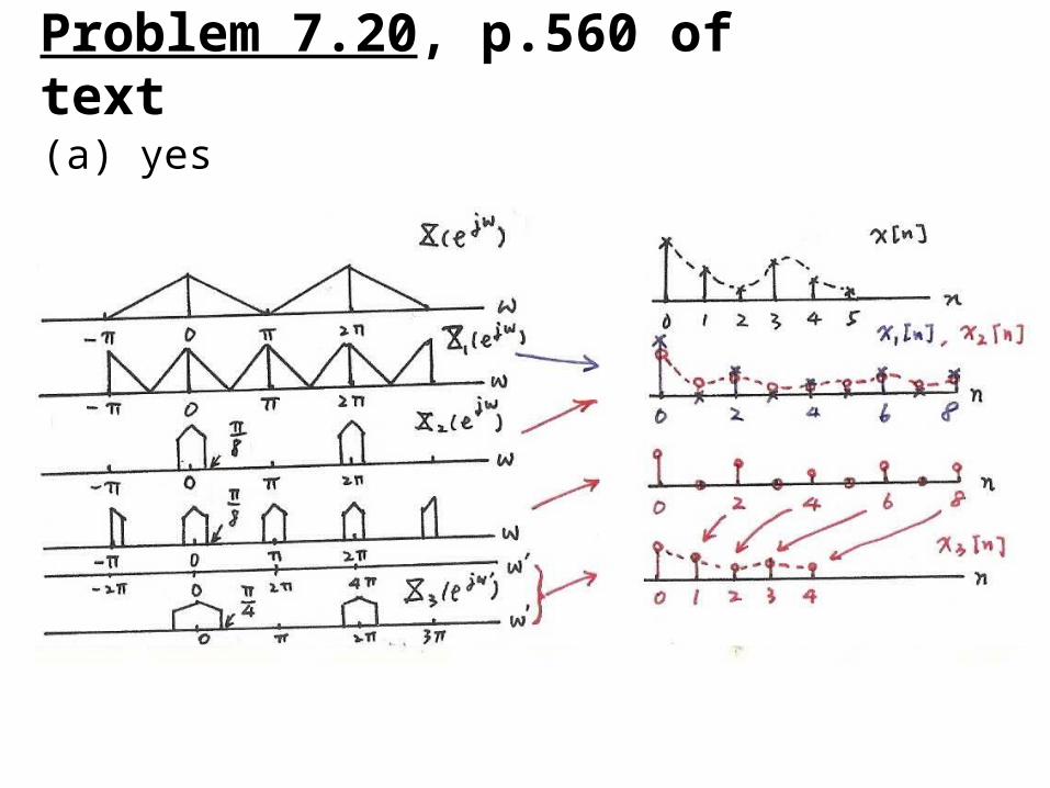
Problem 7.20, p.560 of text
(a) yes

Problem 7.20, p.560 of text
(b) no

Problem 7.23, p.562 of text
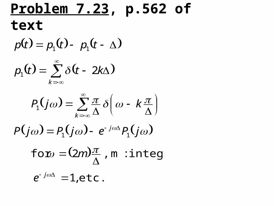
Problem 7.23, p.562 of text
etc. ,1
integer:m , 2for
2
11
1
1
11
j
j
k
k
e
m
jPejPjP
kjP
kttp
tptptp
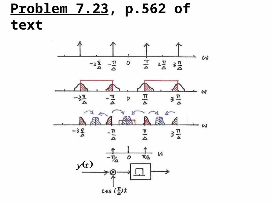
Problem 7.23, p.562 of text
ty
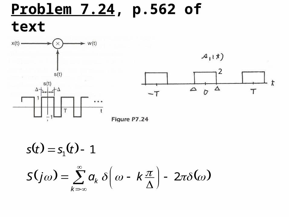
Problem 7.24, p.562 of text
2
11
kajS
tsts
kk
2
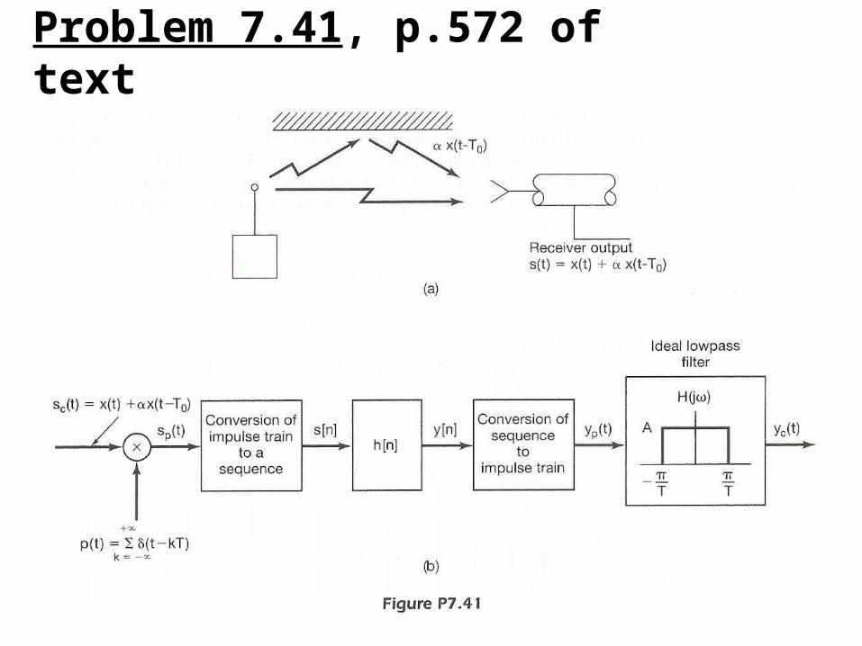
Problem 7.41, p.572 of text
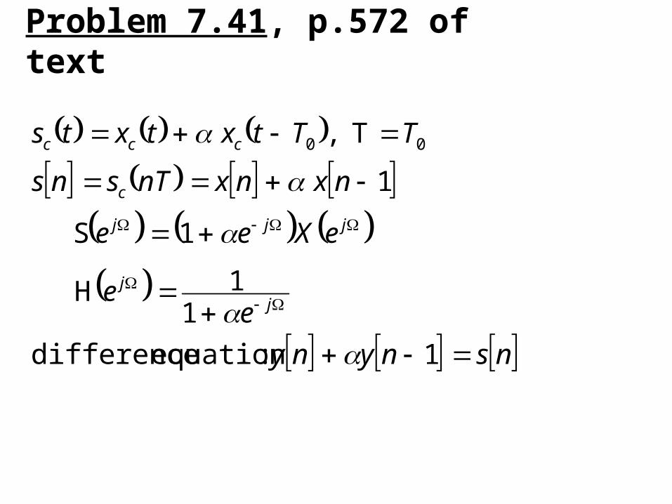
Problem 7.41, p.572 of text
nsnyny
ee
eXee
nxnxnTsns
TTtxtxts
jj
jjj
c
ccc
1 :equation difference
11H
1S
1
T , 00
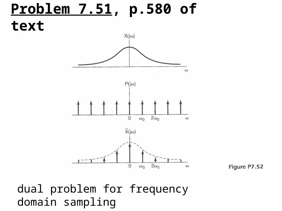
Problem 7.51, p.580 of text
dual problem for frequency domain sampling
Related Documents