7. The Energy Cycle - Colorado State Universitykiwi.atmos.colostate.edu/group/dave/at605pdf/Chapter_7.pdf · negative quantity A=H gs ... concept of available potential energy, ...

7. The Energy Cycle

Copyright 2013, David A. Randall

Available potential energy

We showed in Chapter 4 that, under dry adiabatic and frictionless processes,

ddt

cvΤ + φ +Κ( )ρdVV∫ = 0 .

(1)Here the integral is over the mass of the whole atmosphere. Also recall from Chapter 4 that, for each vertical column, hydrostatic balance implies that the vertically integrated sum of the mass-weighted internal and potential energies is equal to the vertical integral of the mass-weighted enthalpy, i.e.,

cvΤ + φ( )dp0

ps

∫ = cpΤ dp0

ps

∫ .

(2)Let H and Κ be the total (mass integrated) enthalpy and kinetic energy of the entire atmosphere. It follows from (1) and (2) that H +Κ is invariant, under dry-adiabatic frictionless processes, i.e.,

ddt

H +Κ( ) = 0 .

(3)Imagine that we have the power to spatially rearrange the mass of the atmosphere at will, adiabatically and reversibly. As the parcels move, their entropy and potential temperature do not change, but their enthalpy and temperature do change. Suppose that we are given a state of the atmosphere - a set of maps, if you like. Starting from this given state, we move parcels around adiabatically and without friction until we find the unique state of the system that minimizes H . This means that we have reduced H as much as possible from its value in the given state. Because H +Κ does not change,Κ is maximized in this special state, which Lorenz (1955) called the “reference state,” and which we will call the “A-state.”

! Revised Thursday, March 28, 2013! 1

An Introduction to the General Circulation of the Atmosphere

You should prove for yourself that the mass-integrated potential energy of the entire atmosphere is lower in the A-state than in the given state. This means that the center of gravity of the atmosphere descends as the atmosphere passes from the given state to the A-state.

An adiabatic process that reduces H will also reduce the total potential energy of the atmospheric column. The non-kinetic energy that “disappears” in this process is converted into kinetic energy. Therefore, we can say that an adiabatic process that reduces H will tend to increase the kinetic energy of the atmosphere. Two very important processes of this type are convection and baroclinic instability.

In passing from the given state to the A-state we have

Hgs → Hmin ,

Κ gs →Κ gs + Hgs − Hmin( ) =Κmax ,

(4)where Hmin is the value of H in the A-state, and subscript gs denotes the given state. The non-

negative quantity

A = Hgs − Hmin ≥ 0(5)

is called the “available potential energy,” or APE. The APE was first defined by Lorenz (1955; see Fig. 7.1). Eq. (5) gives the fundamental definition of the APE.

Notice that the APE is a property of the entire atmosphere; it cannot be rigorously defined for a portion of the atmosphere, although the literature does contain studies in which the APE is

Figure 7.1: Prof. Edward N. Lorenz, who proposed the concept of available potential energy, and has published a great deal of additional very fundamental research in the atmospheric sciences and the relatively new science of nonlinear dynamical systems.



computed, without rigorous justification, for a portion of the atmosphere, e.g., the Northern Hemisphere.

The A-state is invariant under adiabatic processes, because it depends only on the probability distribution of θ over the mass, rather than on any particular spatial arrangement of the air. Therefore

dAdt

= ddt

Hgs − Hmin( )

=dHgs

dt.

(6)Then (3) implies that

ddt

A +Κ( ) = 0 .

(7)The sum of the available potential and kinetic energies is invariant under adiabatic frictionless processes. This means that such processes only convert between A and K .

The APE of the A-state itself is obviously zero.

In order to compute A , we have to find the A-state and its (minimum) enthalpy. We can deduce the properties of the A-state as follows: There can’t be any horizontal pressure gradients in the A-state, because if there were K could increase. It follows that the potential temperature must be constant on isobaric surfaces, which is of course equivalent to the statement that p is

constant on θ surfaces. This means that both the variance of θ on isobaric surfaces and the variance of p on isentropic surfaces are measures of the APE. There can be no static instability

∂θ / ∂z < 0( ) in the A-state for a similar reason. From these considerations we conclude that, in

the A-state,θ and Τ are uniform on each pressure-surface, or equivalently that p is uniform on

each θ -surface, and also that θ does not decrease upward.

It would appear, and to a large extent it is true, that in passing from the given state to the A-state, no mass can cross an isentropic surface, because we allow only dry adiabatic processes for which θ = 0 . This implies that pθ , the average pressure on an isentropic surface, cannot

change as we pass to the A-state. There is an important exception to this rule, however. If ∂θ / ∂z < 0 in the given state, then the average pressure on an isentropic surface will be different in the A-state. This case of static instability is discussed below.



A complication arises: What about θ -surfaces that intersect the ground in the given state? These are treated as though they continue along the ground, as shown in Fig. 7.2, Because the “layers” between the isentropic surfaces that are following the ground contain no mass, they have no effect on the physics. They are called “massless layers.” Where a θ -surface intersects the Earth’s surface, the pressure is p = pS .

As shown by the heavy arrows in Fig. 7.3, warm air must rise (move to lower pressure) and cold air must sink (move to higher pressure) to pass from the given state to the A-state. This

Figure 7.2: Sketch illustrating the concept of “massless layers.”

Lower boundary

θ2

θ2 θ

1θ1

Figure 7.3: Sketch illustrating the transition from a given state to the A-state. Here p increases

downward and we assume that θ3 >θ2 >θ1 , which means that the atmosphere is statically stable.

θ2

θ1

θ3

θ3

θ2

θ1

given state A-state

p(θ ) ≠ constant p(θ ) = constant

H = Hgs> H

minH = H

min

Hgs −Hmin≡ APE



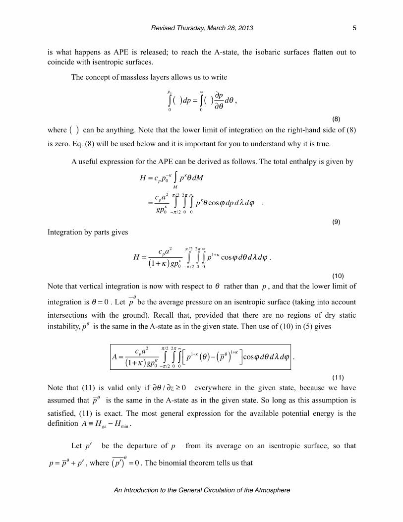
is what happens as APE is released; to reach the A-state, the isobaric surfaces flatten out to coincide with isentropic surfaces.

The concept of massless layers allows us to write

( )dp0

ps

∫ = ( ) ∂p∂θ

dθ0

∞

∫ ,

(8)where ( ) can be anything. Note that the lower limit of integration on the right-hand side of (8)

is zero. Eq. (8) will be used below and it is important for you to understand why it is true.

A useful expression for the APE can be derived as follows. The total enthalpy is given by

H = cp p0−κ pκθ dM

M∫

=cpa

2

gp0κ pκθ cosϕ dpdλ dϕ

0

ps

∫0

2π

∫−π /2

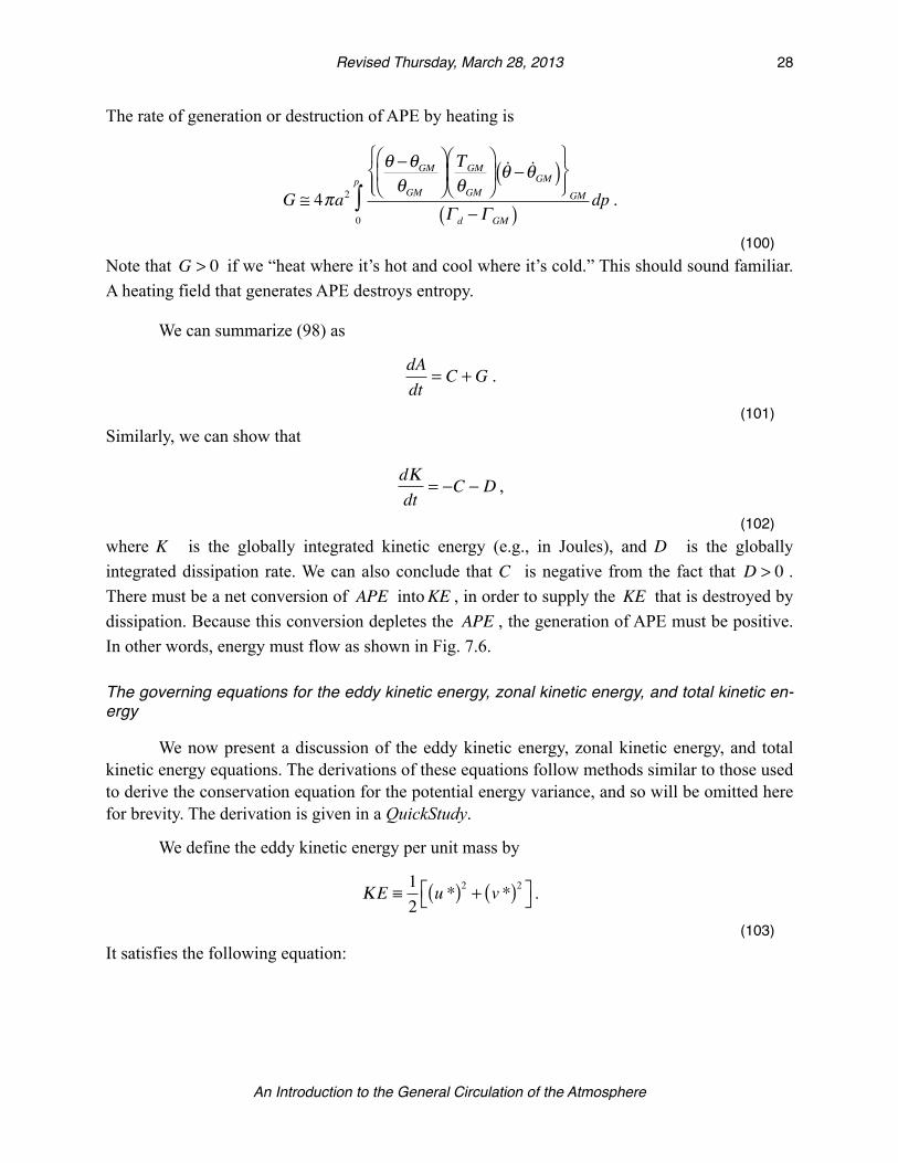
π /2

∫ .

(9)Integration by parts gives

H =cpa

2

1+κ( )gp0κp1+κ cosϕ dθ dλ dϕ

0

∞

∫0

2π

∫−π /2

π /2

∫ .

(10)Note that vertical integration is now with respect to θ rather than p , and that the lower limit of

integration is θ = 0 . Let pθ

be the average pressure on an isentropic surface (taking into account

intersections with the ground). Recall that, provided that there are no regions of dry static instability, pθ is the same in the A-state as in the given state. Then use of (10) in (5) gives

A =cpa

2

1+κ( )gp0κp1+κ θ( )− pθ( )1+κ⎡

⎣⎤⎦cosϕ dθ dλ dϕ

0

∞

∫0

2π

∫−π /2

π /2

∫ .

(11)Note that (11) is valid only if ∂θ / ∂z ≥ 0 everywhere in the given state, because we have assumed that pθ is the same in the A-state as in the given state. So long as this assumption is

satisfied, (11) is exact. The most general expression for the available potential energy is the definition A ≡ Hgs − Hmin .

Let ′p be the departure of p from its average on an isentropic surface, so that

p = pθ + ′p , where ′p( )θ= 0 . The binomial theorem tells us that



p1+κ θ( ) = pθ( )1+κ 1+ ′p θ( )pθ

⎡⎣⎢

⎤⎦⎥

1+κ

= pθ( )1+κ 1+ 1+κ( ) ′p θ( )pθ +

κ 1+κ( )2!

′p θ( )pθ

⎡⎣⎢

⎤⎦⎥

2

+ ⋅⋅⋅⎧⎨⎪

⎩⎪

⎫⎬⎪

⎭⎪.

(12)Lorenz used (12) to write

p1+κ θ( ) ≅ pθ( )1+κ 1+κ 1+κ( )2!

′p θ( )pθ

⎡⎣⎢

⎤⎦⎥

2⎧⎨⎪

⎩⎪

⎫⎬⎪

⎭⎪,

(13)and he showed that this is actually a pretty good approximation. Substitution of (13) into (11) gives

A ≅Ra2

2gp0κ pθ( )1+κ ′p

pθ

⎛⎝⎜

⎞⎠⎟

2

cosϕ dθ dλ dϕ0

∞

∫0

2π

∫−π /2

π /2

∫ .

(14)Because he wanted to express his results in terms of perturbations on isobaric surfaces,

rather than pressure perturbations on isentropic surfaces, Lorenz also used

′p θ( ) ≅ ′θ p( ) ∂p∂θ

≅ ′θ p( ) ∂pθ

∂θ

= ′θ p( ) ∂θ∂p

⎛⎝⎜

⎞⎠⎟

−1

,

(15)where, as before, ′p represents the departure of p from its global average on an isentropic

surface, and ′θ represents the departure of θ from θ , its global average on a p -surface.

Substitution of (15) into (14) gives

A ≅ Ra2

2gp0κ

θ 2

p1−κ( ) − ∂θ∂p

⎛⎝⎜

⎞⎠⎟

′θ p( )θ

⎡⎣⎢

⎤⎦⎥

2

cosϕ dpdλ dϕ0

ps

∫0

2π

∫−π /2

π /2

∫ .

(16)Here the independent variable used for vertical integration has been changed from θ to p , and

correspondingly an overbar now represents an average on an isobaric surface, and a prime denotes the departure from an average on an isobaric surface. Eq. (16) says that the available



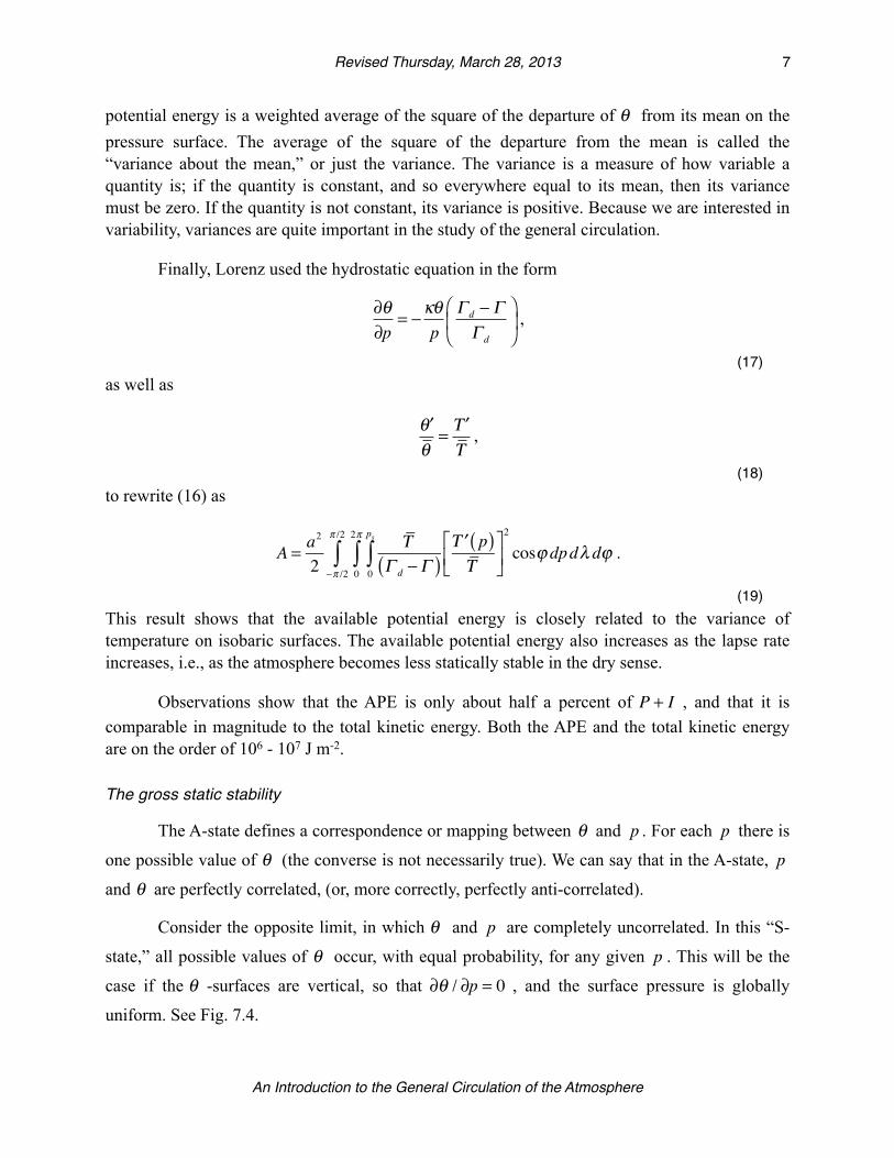
potential energy is a weighted average of the square of the departure of θ from its mean on the pressure surface. The average of the square of the departure from the mean is called the “variance about the mean,” or just the variance. The variance is a measure of how variable a quantity is; if the quantity is constant, and so everywhere equal to its mean, then its variance must be zero. If the quantity is not constant, its variance is positive. Because we are interested in variability, variances are quite important in the study of the general circulation.

Finally, Lorenz used the hydrostatic equation in the form

∂θ∂p

= −κθp

Γ d − ΓΓ d

⎛

⎝⎜

⎞

⎠⎟ ,

(17)as well as

′θθ

= ′ΤΤ

,

(18)to rewrite (16) as

A = a2

2Τ

Γ d −Γ( )′Τ p( )Τ

⎡⎣⎢

⎤⎦⎥

2

cosϕ dpdλ dϕ0

ps

∫0

2π

∫−π /2

π /2

∫ .

(19)This result shows that the available potential energy is closely related to the variance of temperature on isobaric surfaces. The available potential energy also increases as the lapse rate increases, i.e., as the atmosphere becomes less statically stable in the dry sense.

Observations show that the APE is only about half a percent of P + I , and that it is comparable in magnitude to the total kinetic energy. Both the APE and the total kinetic energy are on the order of 106 - 107 J m-2.

The gross static stability

The A-state defines a correspondence or mapping between θ and p . For each p there is

one possible value of θ (the converse is not necessarily true). We can say that in the A-state, p

and θ are perfectly correlated, (or, more correctly, perfectly anti-correlated).

Consider the opposite limit, in which θ and p are completely uncorrelated. In this “S-

state,” all possible values of θ occur, with equal probability, for any given p . This will be the

case if the θ -surfaces are vertical, so that ∂θ / ∂p = 0 , and the surface pressure is globally

uniform. See Fig. 7.4.



To see why the surface pressure must be globally uniform in the S-state, suppose that there were variations in the surface pressure in the S-state (independent of height at each location). If the surface pressure varies geographically, we can say that it varies with θ . As an example, suppose that, in the S-state, for θ = θ1 the surface pressure is 900 mb. Then if I tell you

that the pressure where I am is 1000 mb, you know that my θ cannot be θ1 , i.e., you have a clue

that will help you (at least a little bit) to figure out my θ . This shows that variations of the surface pressure in the S-state would violate the rule that θ and p are completely uncorrelated

in the S-state. Therefore, the surface pressure must be uniform in the S-state.

A globally uniform surface pressure seems reasonable enough in the absence of topography, but it is a very strange state when topography is present. Lorenz (personal communication, 2003) suggested an alternative definition of the S-state, in which the surface pressure is allowed to vary in a simple and natural way with the surface height, but the potential temperature is spatially distributed so that it is uncorrelated with the surface height (and, therefore, uncorrelated with the surface pressure).

We pass from the given state to the S-state by way of an adiabatic process; it follows that the S-state itself is invariant under adiabatic processes. The gross static stability is defined to be the enthalpy of the S-state minus the enthalpy of the given state, i.e.,

S ≡ HS− state − Hgs .

(20)

The total enthalpy of the S-state is given by

Figure 7.4: Sketch illustrating the transition from a given state to the S state used to define the gross static stability.

θ2

θ1

θ3

θ3

θ2θ

1

given state S-state

∂θ

∂p≠ 0

∂θ

∂p= 0

pS varies pS uniform



HS−state = cp p0−κ pκθ dM

M∫

=cpa

2

gp0κ pκθ cosϕ dpdλ dϕ

0

ps∫0

2π

∫−π /2

π /2

∫

=cpa

2

gp0κ θ

0

2π

∫ pκ dp0

ps∫( )dλ cosϕ dϕ−π /2

π /2

∫

=cpa

2

gp0κ θ pS

1+κ

1+κ⎛⎝⎜

⎞⎠⎟dλ cosϕ dϕ

0

2π

∫−π /2

π /2

∫ .

(21)At this point, we can consider each of the two definitions of the S-state that were

mentioned above. If the surface pressure is globally uniform in the S-state, then we can simply replace pS by pS in (21), and write

HS−state =cpa

2

gp0κ θ

pS( )1+κ1+κ

⎡

⎣

⎢⎢

⎤

⎦

⎥⎥dλ cosϕ dϕ

0

2π

∫−π /2

π /2

∫

=cpa

2

gp0κ

pS( )1+κ1+κ

⎡

⎣

⎢⎢

⎤

⎦

⎥⎥

θ dλ cosϕ dϕ0

2π

∫−π /2

π /2

∫

=cp4πa

4

gp0κ

pS( )1+κ θ1+κ

⎡

⎣

⎢⎢

⎤

⎦

⎥⎥,

(22)

where pS is the globally averaged surface pressure, which is the same in the given state and the

S-state, and θ is the globally averaged potential temperature in the S-state, which is the same as the mass-averaged potential temperature in the given state.

Alternatively, if θ is uncorrelated with p1+κS in the the S-state, then it follows

immediately from (21) that

HS−state =cp4πa

4

gp0κ

pS( )1+κ θ1+κ

⎡

⎣

⎢⎢

⎤

⎦

⎥⎥

.

(23)We conclude that the two definitions of the S-state actually give exactly the same result for HS−State .

Now we show why S is called the “gross static stability.” Eq. (21) can also be written as



HS− state =

cpa2

gp0κ

pκ

p0κ

⎛⎝⎜

⎞⎠⎟

θ dp0

ps∫( )cosϕ dλ dϕ0

2π

∫−π /2

π /2

∫ ,

(24)where

pκ ≡

pS( )κ1+κ

.

(25)

In (24), the integral over pressure simply amounts to multiplication by pS , because θ is

independent of height in the S-state. The integral of the potential temperature over the entire mass of the atmosphere must be exactly the same for the given state and the S-state, i.e.,

a2

gθ dp

0


2π

∫−π /2

π /2

∫⎡

⎣⎢

⎤

⎦⎥

given state

= a2

gθ dp

0

ps∫⎛⎝⎞⎠ cosϕ dλ dϕ

0

2π

∫−π /2

π /2

∫⎡

⎣⎢

⎤

⎦⎥

S-state

.

(26)This allows us to rewrite (24) as

HS− state =cpa

2

gpκ

p0κ

⎛⎝⎜

⎞⎠⎟

θ dp0


2π

∫−π /2

π /2

∫⎡

⎣⎢

⎤

⎦⎥

given state

.

(27)Now substitute (27) into (20), to obtain

S ≡cpa

2

gpκ

p0κ

⎛⎝⎜

⎞⎠⎟

θ dp0


2π

∫−π /2

π /2

∫⎡

⎣⎢

⎤

⎦⎥

given state

−cpa

2

gp0κ pκθ

0

ps∫ cosϕ dpdλ dϕ0

2π

∫−π /2

π /2

∫ .

(28)This can be rearranged to

S ≡cpa

2

gp0κ pκ − pκ( )θ dp

0

ps∫⎡⎣⎢⎤⎦⎥cosϕ dλ dϕ

0

2π

∫−π /2

π /2

∫⎧⎨⎪

⎩⎪

⎫⎬⎪

⎭⎪given state

.

(29)Integration by parts gives

S ≡cpa

2

gp0κ 1+κ( ) pS( )κ p − p1+κ⎡

⎣⎢⎤⎦⎥ − ∂θ

∂p⎛⎝⎜

⎞⎠⎟dp

0

ps∫⎡

⎣⎢

⎤

⎦⎥cosϕ dλ dϕ

0

2π

∫−π /2

π /2

∫⎧⎨⎪

⎩⎪

⎫⎬⎪

⎭⎪given state

,

(30)



which shows that S is a weighted average of −∂θ / ∂p( ) ; it is, therefore, a measure of the static

stability, and this accounts for its name. Like the available potential energy, the gross static stability is defined only for the atmosphere as a whole.

The globally averaged surface pressure and the probability distribution of θ are invariant under adiabatic processes. This means that the S-state is invariant as well. Because S is defined as the difference between the total enthalpy of the S-state and the total enthalpy of the given state, we can write

dSdt

= −dHdt

.

(31)

Since ddt

H +Κ( ) = 0 , it follows from (31) that

dSdt

=dΚdt

.

(32)This shows that when Κ is produced by conversion from APE, the gross static stability increases. In passing from the given state to the A-state, the available potential energy decreases, and the kinetic energy and gross static stability both increase. Isn’t that what you would expect?

Examples: The available potential energies of three simple systems

Available potential energy can arise in several different ways. We now consider three idealized examples, each of which illustrates a “source” of available potential energy in pure, unadulterated form.

Example #1: The APE associated with static instability

As an example, consider a simple system containing two parcels of equal mass. In the given state, parcels with potential temperature θ1 and θ2 reside at pressures p1 and p2 ,

respectively. We assume that θ1 < θ2 and p1 < p2 , so that the given state is statically unstable.

The enthalpy per unit mass of parcel i is cpθipip0

⎛⎝⎜

⎞⎠⎟

κ

. If the parcels are interchanged (or

“swapped”) so that parcel number 2 goes to pressure p1 and vice versa, the change in the total

enthalpy per unit mass is



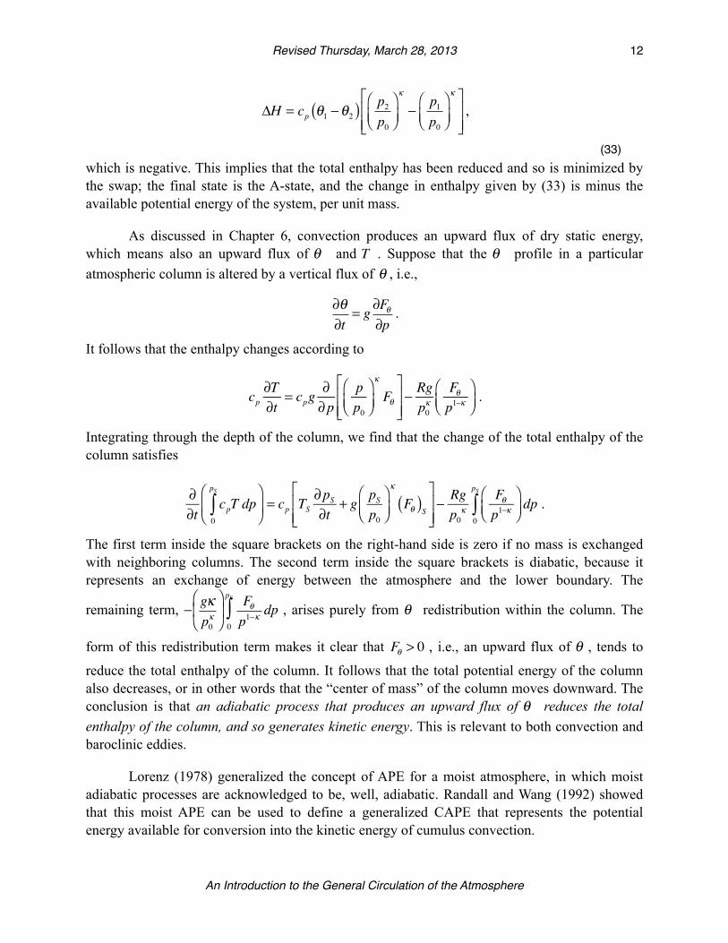
ΔH = cp θ1 −θ2( ) p2p0

⎛⎝⎜

⎞⎠⎟

κ

−p1p0

⎛⎝⎜

⎞⎠⎟

κ⎡

⎣⎢⎢

⎤

⎦⎥⎥

,

(33)which is negative. This implies that the total enthalpy has been reduced and so is minimized by the swap; the final state is the A-state, and the change in enthalpy given by (33) is minus the available potential energy of the system, per unit mass.

As discussed in Chapter 6, convection produces an upward flux of dry static energy, which means also an upward flux of θ and T . Suppose that the θ profile in a particular atmospheric column is altered by a vertical flux of θ , i.e.,

∂θ∂t

= g ∂Fθ∂p

.

It follows that the enthalpy changes according to

cp∂T∂t

= cpg∂∂p

pp0

⎛⎝⎜

⎞⎠⎟

κ

Fθ⎡

⎣⎢⎢

⎤

⎦⎥⎥− Rgp0κ

Fθp1−κ

⎛⎝⎜

⎞⎠⎟

.

Integrating through the depth of the column, we find that the change of the total enthalpy of the column satisfies

∂∂t

cpT dp0

pS

∫⎛

⎝⎜⎞

⎠⎟= cp TS

∂pS∂t

+ g pSp0

⎛⎝⎜

⎞⎠⎟

κ

Fθ( )S⎡

⎣⎢⎢

⎤

⎦⎥⎥− Rgp0

κFθp1−κ

⎛⎝⎜

⎞⎠⎟0

pS

∫ dp .

The first term inside the square brackets on the right-hand side is zero if no mass is exchanged with neighboring columns. The second term inside the square brackets is diabatic, because it represents an exchange of energy between the atmosphere and the lower boundary. The

remaining term, − gκp0κ

⎛

⎝⎜

⎞

⎠⎟

Fθp1−κ0

pS

∫ dp , arises purely from θ redistribution within the column. The

form of this redistribution term makes it clear that Fθ > 0 , i.e., an upward flux of θ , tends to

reduce the total enthalpy of the column. It follows that the total potential energy of the column also decreases, or in other words that the “center of mass” of the column moves downward. The conclusion is that an adiabatic process that produces an upward flux of θ reduces the total enthalpy of the column, and so generates kinetic energy. This is relevant to both convection and baroclinic eddies.

Lorenz (1978) generalized the concept of APE for a moist atmosphere, in which moist adiabatic processes are acknowledged to be, well, adiabatic. Randall and Wang (1992) showed that this moist APE can be used to define a generalized CAPE that represents the potential energy available for conversion into the kinetic energy of cumulus convection.



Example #2: The APE associated with meridional temperature gradients

As a second example consider an idealized planet, with no orography and a uniform surface pressure in the given state. Suppose that the potential temperature of the given state is a function of latitude only:

θgs µ( ) = θ0 1− ΔHµ2( ) ,

(34)Here ΔH is a constant, and µ ≡ sinϕ . The subscript “gs” denotes the given state. Eq. (34) is the

same meridional distribution of θ as used for θE in Chapter 5. Recall that for realistic states

0 < ΔH < 1 . The available potential energy of this idealized given state arises solely from the

meridional temperature gradient. To obtain an expression for the available potential energy of the given state, we need to compute the total enthalpies of the given state and the A-state, and subtract them. The first step is to find the A-state. Note that, in this idealized example, the given state is identical to the S-state.

The mass in a latitude belt of width dϕ is:

dm = 2 2πacosϕ( ) pSg

⎛

⎝⎜

⎞

⎠⎟ adϕ( )

= 4πa2

gpSdµ ,

(35)where µ ≡ sinϕ , and dµ = cosϕdϕ . In (35) the leading factor of two is included because we

have symmetry across the equator, so when we increment latitude in one hemisphere we actually pick up mass from two “rings” of air, one in each hemisphere. The rate of change of θ as we add mass is:

dθdm

=dθdµ

⎛⎝⎜

⎞⎠⎟ gs

dmdµ

⎛⎝⎜

⎞⎠⎟

−1

.

(36)Combining (35) and (36), we get

dθdm

=g

4πa2 pSdθdµ

⎛⎝⎜

⎞⎠⎟ gs

.

(37)In the A-state, the θ -surfaces are flat, and the increment of mass between two θ -surfaces

is



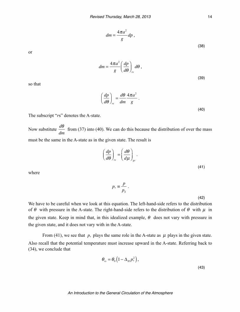
dm =4πa2

gdp ,

(38)or

dm =4πa2

gdpdθ

⎛⎝⎜

⎞⎠⎟ rsdθ ,

(39)so that

dpdθ

⎛⎝⎜

⎞⎠⎟ rs

=dθdm

4πa2

g.

(40)The subscript “rs” denotes the A-state.

Now substitute dθdm

from (37) into (40). We can do this because the distribution of over the mass

must be the same in the A-state as in the given state. The result is

dpdθ

⎛⎝⎜

⎞⎠⎟ rs

=dθdµ

⎛⎝⎜

⎞⎠⎟ gs

.

(41)where

p* ≡ppS

.

(42)We have to be careful when we look at this equation. The left-hand-side refers to the distribution of θ with pressure in the A-state. The right-hand-side refers to the distribution of θ with µ in

the given state. Keep in mind that, in this idealized example, θ does not vary with pressure in the given state, and it does not vary with in the A-state.

From (41), we see that p* plays the same role in the A-state as µ plays in the given state.

Also recall that the potential temperature must increase upward in the A-state. Referring back to (34), we conclude that

θrs = θ0 1− ΔH p*2( ) ,

(43)



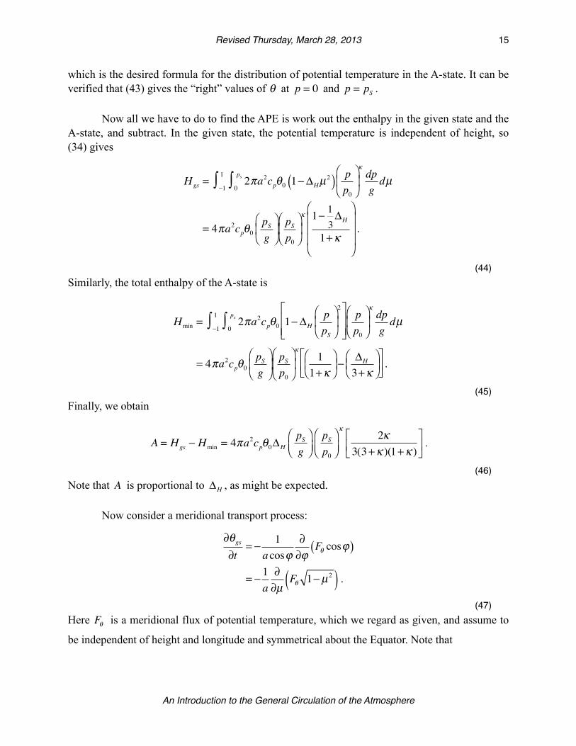
which is the desired formula for the distribution of potential temperature in the A-state. It can be verified that (43) gives the “right” values of θ at p = 0 and p = pS .

Now all we have to do to find the APE is work out the enthalpy in the given state and the A-state, and subtract. In the given state, the potential temperature is independent of height, so (34) gives

Hgs = 2πa2cpθ0 1− ΔHµ2( ) p

p0

⎛

⎝⎜

⎞

⎠⎟κdpgdµ

0

ps∫−1

1∫

= 4πa2cpθ0pSg

⎛

⎝⎜

⎞

⎠⎟pSp0

⎛

⎝⎜

⎞

⎠⎟κ 1− 1

3ΔH

1+κ

⎛

⎝

⎜⎜⎜

⎞

⎠

⎟⎟⎟.

(44)Similarly, the total enthalpy of the A-state is

Hmin = 2πa2cpθ0 1− ΔHppS

⎛

⎝⎜

⎞

⎠⎟2⎡

⎣⎢⎢

⎤

⎦⎥⎥pp0

⎛

⎝⎜

⎞

⎠⎟κdpgdµ

0

ps∫−1

1∫

= 4πa2cpθ0pSg

⎛

⎝⎜

⎞

⎠⎟pSp0

⎛

⎝⎜

⎞

⎠⎟κ

11+κ⎛⎝⎜

⎞⎠⎟−

ΔH

3+κ⎛⎝⎜

⎞⎠⎟

⎡⎣⎢

⎤⎦⎥.

(45)Finally, we obtain

A = Hgs − Hmin = 4πa2cpθ0ΔH

pSg

⎛⎝⎜

⎞⎠⎟

pSp0

⎛⎝⎜

⎞⎠⎟

κ2κ

3(3+κ )(1+κ )⎡⎣⎢

⎤⎦⎥

.

(46)Note that A is proportional to ΔH , as might be expected.

Now consider a meridional transport process:

∂θgs

∂t= − 1

acosϕ∂∂ϕ

Fθ cosϕ( )

= − 1a

∂∂µ

Fθ 1−µ2( ) .(47)

Here Fθ is a meridional flux of potential temperature, which we regard as given, and assume to

be independent of height and longitude and symmetrical about the Equator. Note that



Fθ = 0 at both poles.

(48)Assume that the surface pressure does not change with time at any latitude. What is the time rate of change of the APE associated with this meridional redistribution of potential temperature?

To answer this question, first note that the time rate of change of the total enthalpy of the given state is:

∂Hgs

∂t= 2πa2cp

∂θ∂t

⎛⎝⎜

⎞⎠⎟pp0

⎛

⎝⎜

⎞

⎠⎟κdpg0

ps∫−1

1∫

=2πa2cp1+κ( )

pSg

⎛

⎝⎜

⎞

⎠⎟pSp0

⎛

⎝⎜

⎞

⎠⎟κ

∂θ∂tdµ

−1

1∫

= −2πa2cp1+κ( )

pSg

⎛

⎝⎜

⎞

⎠⎟pSp0

⎛

⎝⎜

⎞

⎠⎟κ

1acosϕ

∂∂ϕ

Fθ cosϕ( )cosϕ dϕ−π2

π2∫

= 0 .(49)

Here we have used the facts that ∂θ / ∂t is independent of height and that pS is independent of

latitude, and we have substituted from (47). According to (49), the specified transport process has no effect on the total enthalpy of the given state. The reason is that the average θ on each pressure surface is unchanged, and it follows that the average temperature on each pressure surface is unchanged.

The meridional transport process can, however, alter the total enthalpy of the A-state. Here again there is a possibility of confusion. As already mentioned, the specified meridional transport process does not alter the average value of θ on a pressure surface. This statement seems to imply that the process is isentropic, and we already know that isentropic processes do not alter the A-state. The entropy is proportional to ln θ( ) , however, and the average value of

ln θ( ) is altered by the transport process. Another point of view is that generally speaking the

specified transport process is not reversible. For example, Fθ if is a downgradient flux due to

diffusive mixing, then it could, in principle, homogenize θ throughout the entire atmosphere. This process would clearly be irreversible. Following such homogenization, the A-state would be the same as the (homogenized) given state and would, therefore, be different from the A-state found above.

From (49), it follows that

dAdt

= −dHmin

dt.

(50)



Now recall that, based on comparison of (34) and (43), p* plays the same role in the A-state as

µ plays in the given state. In particular, p* = 1 (the surface) corresponds to µ = 1 (the pole), and

p* = 0 (the “top of the atmosphere”) corresponds to µ = 0 (the Equator). Our goal is to

determine the time-rate of change of θ in the A-state at a particular instant, namely, the time when the distribution of θ satisfies (34) [and (43)], and the time-rate-of-change of θ in the given state satisfies (47). We can find the time-rate-of-change of θ in the A-state at this instant by going to our expression for the time-rate-of-change of θ in the given state, and simply replacing µ by p* , everywhere. The time-rate-of-change of θ in the A-state thus satisfies

∂θrs

∂t= −

1a

∂∂p*

Fθ 1− p*2( ) .

(51)Again there is a possibility of confusion. We have specified that Fθ is not a function of

height, although of course it does depend on latitude. It would thus appear that we can pull Fθ

out of the derivative in (51), but this is not correct. The reason is that, when µ was replaced by

p* we also replaced the µ -dependence of Fθ by a corresponding p* -dependence. Thus, in (51),

Fθ should be regarded as a function of p* , but not as a function of latitude! This is

understandable, because Fθ is acting to change θrs p*( ) . As an example, suppose that Fθ is

symmetric about the Equator, and poleward in both hemispheres, and that ΔH > 0 so that the

poles are in fact colder than the tropics. Then Fθ tends to warm the poles and cool the tropics,

reducing ΔH and, we expect, reducing A . As the tropics cool and the poles warm in the given

state, the A-state evolves in a corresponding way, so that θrs cools aloft and warms at the lower

levels.

We now write the time-rate-of-change of the total enthalpy in the A-state as

∂Hmin

∂t= 2πa2cp

∂θ∂t

⎛⎝⎜

⎞⎠⎟pp0

⎛

⎝⎜

⎞

⎠⎟κdpgdµ

0

ps∫−1

1∫

=4πa2cp pS

gpSp0

⎛

⎝⎜

⎞

⎠⎟κ

∂θ∂t

⎛⎝⎜

⎞⎠⎟ p*( )κ dp*0

1∫

=4πa2cp pS

gpSp0

⎛

⎝⎜

⎞

⎠⎟κ

∂∂p*

Fθ 1− p*2( )⎡

⎣⎢

⎤

⎦⎥ p*

κ dp*0

1∫ .

(52)We cannot do the integral on the last line of (52), because the form of Fθ has not been specified.

The last step would be to substitute (52) into (50).



Example #3: The APE associated with surface pressure variations

The third example is designed to illustrate that APE can occur in the presence of surface pressure gradients, even when there are no potential temperature gradients; this is analogous to the APE of shallow water with a non-uniform free-surface height. To explore this possibility in a simple framework, consider a planet with an atmosphere of uniform potential temperature, θ0 .

The surface pressure, pS λ,ϕ( ) , is given as a function of longitude, λ and latitude ϕ . For

simplicity we assume that the Earth’s surface is flat, although a similar but more complicated analysis can be developed for the case of arbitrary surface topography.

We begin with (5), the basic definition of the APE. The total enthalpy satisfies

H = cpθpp0

⎛⎝⎜

⎞⎠⎟

κdpgacosϕ dλadϕ

0

ps

∫0

2π

∫−π2

π2∫ .

(53)Because θ = θ0 everywhere in this example, we can simplify (53) considerably:

H =cpθ0a

2

g 1+κ( ) p0κpS1+κ cosϕ dλ dϕ

0

2π

∫−π2

π2∫ .

(54)Eq. (54) can be applied to both the given state and the A-state, so that the APE is given by

A =cpθ0a

2

g 1+κ( ) p0κpS( )gs

1+κ − pS( )rs1+κ⎡

⎣⎤⎦cosϕ dλ dϕ

0

2π

∫−π2

π2∫ .

(55)Before we can evaluate the double integrals in (55), we must substitute for pS λ,ϕ( )⎡⎣ ⎤⎦gs and

pS λ,ϕ( )⎡⎣ ⎤⎦rs . The former is assumed to be known. Our problem thus reduces to finding

pS λ,ϕ( )⎡⎣ ⎤⎦rs . This is very simple, because (since by assumption there are no mountains) the

surface pressure is globally uniform in the A-state, and equal to the globally averaged surface pressure in the given state. We denote this globally averaged surface pressure by pS , and rewrite

(55) as

A =cpθ0a

2

g 1+κ( ) p0κpS( )gs

1+κ − pS( )rs

1+κ⎡⎣⎢

⎤⎦⎥cosϕ dλ dϕ

0

2π

∫−π2

π2∫ .

(56)As an exercise, prove that (56) gives A ≥ 0 .



Variance budgets

From (19) we see that the available potential energy is closely related to the variance of temperature or potential temperature on pressure surfaces. We now examine a conversion process that couples the variance associated with the meridional gradient of the zonally averaged potential temperature with the eddy variance of potential temperature. This same process is closely related to the conversion between the zonal available potential energy, AZ , and eddy

available potential energy, AE . The eddy potential temperature variance interacts with the

meridional gradient of the zonally averaged potential temperature through

∂∂t

12

θ*2⎡⎣ ⎤⎦

⎛⎝⎜

⎞⎠⎟ ~

− θ*v*[ ]a

∂∂ϕ

θ[ ] .

(57)The term shown in the right-hand side of (57) is called the “meridional gradient-production term.” There are actually several additional terms; the others are discussed below.

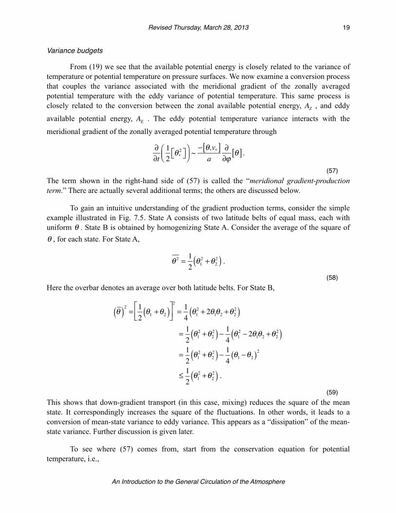
To gain an intuitive understanding of the gradient production terms, consider the simple example illustrated in Fig. 7.5. State A consists of two latitude belts of equal mass, each with uniform θ . State B is obtained by homogenizing State A. Consider the average of the square of θ , for each state. For State A,

θ 2 = 12θ12 +θ2

2( ) .

(58)Here the overbar denotes an average over both latitude belts. For State B,

θ( )2 = 12θ1 +θ2( )⎡

⎣⎢⎤⎦⎥2

= 14θ12 + 2θ1θ2 +θ2

2( )

= 12θ12 +θ2

2( ) − 14 θ12 − 2θ1θ2 +θ2

2( )= 12θ12 +θ2

2( ) − 14 θ1 −θ2( )2

≤ 12θ12 +θ2

2( ) .

(59)This shows that down-gradient transport (in this case, mixing) reduces the square of the mean state. It correspondingly increases the square of the fluctuations. In other words, it leads to a conversion of mean-state variance to eddy variance. This appears as a “dissipation” of the mean-state variance. Further discussion is given later.

To see where (57) comes from, start from the conservation equation for potential temperature, i.e.,



∂θ∂t

+1

acosϕ∂∂λ

uθ( ) + 1acosϕ

∂∂ϕ

vθ cosϕ( ) + ∂∂p

ωθ( ) = θ ,

(60)

and also mass continuity:

1acosϕ

∂u∂λ

+1

acosϕ∂∂ϕ

vcosϕ( ) + ∂ω∂p

= 0 .

(61)Zonally average (60) and (61), to obtain

∂∂t

θ[ ]+ 1acosϕ

∂∂ϕ

vθ[ ]cosϕ( ) + ∂∂p

ωθ[ ] = θ⎡⎣ ⎤⎦ ,

(62)1

acosϕ∂∂ϕ

v[ ]cosϕ( ) + ∂∂p

ω[ ] = 0 .

(63)Subtracting (62) and (63) from (60) and (61), respectively, we find that

Figure 7.5: A simple example to explain the idea of gradient production. State B is obtained by homogenizing State A. In both State A and State B, the average of is. Variance seems to “disappear” in passing from State A to State B. In reality it is converted from the variance of the mean to an eddy variance.

Mixing

State A

State B



∂θ*∂t

+ 1acosϕ

∂∂λ

uθ( ) + 1acosϕ

∂∂ϕ

vθ − vθ[ ]( )cosϕ{ }+ ∂∂p

ωθ − ωθ[ ]( )

= ∂θ*∂t

+ 1acosϕ

∂∂λ

u* θ[ ] + u[ ]θ* + u*θ*( ) + 1acosϕ

∂∂ϕ

v* θ[ ] + v[ ]θ* + v*θ* − v*θ*[ ]( )cosϕ{ }

+ ∂∂p

ω∗ θ[ ] + ω[ ]θ∗ +ω∗θ∗ − ω∗θ∗[ ]( )

= ∂θ*∂t

+ 1acosϕ

∂∂λ

u[ ]θ*( ) + 1acosϕ

∂∂ϕ

v[ ]θ∗( )cosϕ{ }+ ∂∂p

ω[ ]θ∗( )

+ 1acosϕ

∂∂λ

u*θ*( ) + 1acosϕ

∂∂ϕ

v∗θ∗ cosϕ( ) + ∂∂p

ω∗θ*( )

+ 1acosϕ

∂∂λ

u* θ[ ]( ) + 1acosϕ

∂∂ϕ

v∗ θ[ ]cosϕ( ) + ∂∂p

ω∗ θ[ ]( )

− 1acosϕ

∂∂ϕ

v*θ*[ ]cosϕ( ) − ∂∂p

ω∗θ*[ ]( )= θ* ,

(64)1

acosϕ∂u*∂λ

+1

acosϕ∂∂ϕ

v* cosϕ( ) + ∂ω*

∂p= 0 .

(65)To obtain the first equality of (64), we have used

vθ = v[ ] + v*( ) θ[ ] +θ*( ) = v[ ] θ[ ] + v* θ[ ] + v[ ]θ* + v*θ* ,

(66)vθ[ ] = v[ ] θ[ ] + v*θ*[ ] ,

(67)

vθ − vθ[ ] = v* θ[ ] + v[ ]θ* + v*θ* − v*θ*[ ] ,(68)

and so on. We can use (63) and (65) to rewrite (64) as follows:

∂∂t

+u[ ]

acosϕ∂∂λ

+v[ ]a

∂∂ϕ

+ ω[ ] ∂∂p

⎛

⎝⎜

⎞

⎠⎟θ* +

u*acosϕ

∂∂λ

+ v*a

∂∂ϕ

+ω*∂∂p

⎛

⎝⎜

⎞

⎠⎟θ* +

v*a

∂∂ϕ

θ[ ] +ω*∂∂p

θ[ ]

= 1acosϕ

∂∂ϕ

v*θ*[ ]cosϕ( ) + ∂∂p

w*θ*[ ] + θ* .

(69)Multiplying (69) by θ* , and using (65) again, we obtain:



∂∂t

+u[ ]

acosϕ∂∂λ

+v[ ]a

∂dϕ

+ ω[ ] ∂∂p

⎛

⎝⎜

⎞

⎠⎟12θ*2⎛

⎝⎜

⎞⎠⎟

+ 1acosϕ

∂∂λ

u*12θ*2⎛

⎝⎜

⎞⎠⎟

⎧⎨⎩

⎫⎬⎭+ 1acosϕ

∂∂ϕ

v*12θ*2⎛

⎝⎜

⎞⎠⎟cosϕ

⎧⎨⎩

⎫⎬⎭+ ∂∂p

ω*12θ*2⎛

⎝⎜

⎞⎠⎟

⎧⎨⎩

⎫⎬⎭

=θ*1

acosϕ∂∂ϕ

v*θ*[ ]cosϕ( ) + ∂∂p

ω*θ*[ ]⎧⎨⎩

⎫⎬⎭− v*θ*

a∂∂ϕ

θ[ ] −ω*θ*∂∂p

θ[ ] + θ*θ* .

(70)Zonally averaging gives

∂∂t

+v[ ]a

∂dϕ

+ ω[ ] ∂∂p

⎛

⎝⎜

⎞

⎠⎟12θ*2⎡

⎣⎢⎤⎦⎥+ 1acosϕ

∂∂ϕ

v*12θ*2⎛

⎝⎜

⎞⎠⎟

⎡⎣⎢

⎤⎦⎥cosϕ

⎧⎨⎩

⎫⎬⎭+ ∂∂p

ω*12θ*2⎛

⎝⎜

⎞⎠⎟

⎡⎣⎢

⎤⎦⎥

⎧⎨⎩

⎫⎬⎭

= −v*θ*[ ]a

∂∂ϕ

θ[ ] − ω*θ*[ ] ∂∂p

θ[ ] + θ*θ*⎡⎣ ⎤⎦ .

(71)Finally, we can use (63) to rewrite (71) in flux form:

∂∂t

12θ*

2⎡⎣⎢

⎤⎦⎥+ 1acosϕ

∂∂ϕ

v[ ]12

θ*2⎡⎣ ⎤⎦

⎛⎝⎜

⎞⎠⎟ cosϕ⎧

⎨⎩

⎫⎬⎭+ ∂∂p

ω[ ]12

θ*2⎡⎣ ⎤⎦

⎛⎝⎜

⎞⎠⎟

+ 1acosϕ

∂∂ϕ

v*12θ*

2⎛⎝⎜

⎞⎠⎟

⎡⎣⎢

⎤⎦⎥cosϕ

⎧⎨⎩

⎫⎬⎭+ ∂∂p

ω*12θ*

2⎛⎝⎜

⎞⎠⎟

⎡⎣⎢

⎤⎦⎥

⎧⎨⎩

⎫⎬⎭

eddy transport

= −v*θ*[ ]a

∂∂ϕ

θ[ ]− ω*θ*[ ] ∂∂p

θ[ ]gradient prodection

+ θ*θ*⎡⎣ ⎤⎦ .

(72)

According to (72), 12θ*2⎡

⎣⎢⎤⎦⎥

can change due to advection by the mean meridional circulation, or

due to transport by the eddies themselves, or due to “gradient production.”

Eq. (72) governs the eddy variance at a particular latitude. There is also a contribution to the global variance of θ that comes from the meridional and vertical gradients of θ[ ] . To derive

an equation for this part of the global variance of θ , start by using (63) to rewrite (62) as

∂∂t

+v[ ]a

∂∂ϕ

+ ω[ ] ∂∂p

⎛

⎝⎜

⎞

⎠⎟ θ[ ] = − 1

acosϕ∂∂ϕ

v*θ*[ ]cosϕ( ) − ∂∂p

ω*θ*[ ] + θ⎡⎣ ⎤⎦ .

(73)Multiplication by θ[ ] gives



∂∂t

+v[ ]a

∂∂ϕ

+ ω[ ] ∂∂p

⎛

⎝⎜

⎞

⎠⎟12θ[ ]2 = − θ[ ]

acosϕ∂∂ϕ

v*θ*[ ]cosϕ( ) − θ[ ] ∂∂p

ω*θ*[ ]( ) + θ[ ] θ⎡⎣ ⎤⎦ .

(74)This can be rearranged to

∂∂t

+v[ ]a

∂∂ϕ

+ ω[ ] ∂∂p

⎛

⎝⎜

⎞

⎠⎟12θ[ ]2

= − 1acosϕ

∂∂ϕ

θ[ ] v*θ*[ ]cosϕ( ) − ∂∂p

θ[ ] ω*θ*[ ]( ) + v*θ*[ ]a

∂∂ϕ

θ[ ] + ω*θ*[ ] ∂∂p

θ[ ] + θ[ ] θ⎡⎣ ⎤⎦ .

(75)Converting back to flux form, we find that

∂∂t

12θ[ ]2⎛

⎝⎜⎞⎠⎟ +

1acosϕ

∂∂ϕ

v[ ]12 θ[ ]2⎛⎝⎜

⎞⎠⎟ cosϕ

⎧⎨⎩

⎫⎬⎭+ ∂∂p

ω[ ]12 θ[ ]2⎛⎝⎜

⎞⎠⎟

= − 1acosϕ

∂∂ϕ

θ[ ] v*θ*[ ]cosϕ( )− ∂∂p

θ[ ] ω*θ*[ ]( ) + v*θ*[ ]a

∂∂ϕ

θ[ ]+ ω*θ*[ ] ∂∂p

θ[ ]+ θ[ ] θ⎡⎣ ⎤⎦ .

(76)When we add (76) and (72), the gradient production terms cancel. This shows that those

terms represent a “conversion” between 12θ[ ]2 and θ*

2⎡⎣ ⎤⎦ . Note that θ 2⎡⎣ ⎤⎦ = θ[ ]2 + θ*2⎡⎣ ⎤⎦ , i.e., the

zonal average of the square is the sum of the square of the zonal average and the square of the departure from the zonal average. Similarly, θ

θ⎡⎣ ⎤⎦ = θ[ ] θ⎡⎣ ⎤⎦ + θ*θ*⎡⎣ ⎤⎦ . We obtain:

∂∂t

12

θ 2⎡⎣ ⎤⎦⎛⎝⎜

⎞⎠⎟ +

1acosϕ

∂∂ϕ

v[ ]12 θ 2⎡⎣ ⎤⎦ + v*12θ*2⎡

⎣⎢⎤⎦⎥+ θ[ ] v*θ*[ ]⎛

⎝⎜⎞⎠⎟cosϕ

⎧⎨⎩

⎫⎬⎭

+ ∂∂p

ω[ ]12 θ 2⎡⎣ ⎤⎦ + ω*12θ*2⎡

⎣⎢⎤⎦⎥+ θ[ ] ω*θ*[ ]⎛

⎝⎜⎞⎠⎟= θ θ⎡⎣ ⎤⎦ .

(77)Finally, integration of (77) over the entire atmosphere gives

ddt

12

θ 2⎡⎣ ⎤⎦⎛⎝⎜

⎞⎠⎟ dM

M∫ = θ θ⎡⎣ ⎤⎦dM

M∫ .

(78)

Generation of available potential energy, and its conversion into kinetic energy

Earlier we derived (19), Lorenz’s approximate expression for the available potential energy of a statically stable atmosphere, which is repeated here for convenience:



A = a2

2Τ

Γ d −Γ( )′Τ

Τ⎛⎝⎜

⎞⎠⎟2

cosϕ dpdλ dϕ0

ps

∫0

2π

∫−π /2

π /2

∫ .

(79)Recall that in this equation an overbar represents a global mean on a pressure surface, and a prime denotes a departure from the global mean. The APE is an integral of the variance of the temperature about its global mean on pressure surfaces. In the last section, we derived an equation for the time rate of change of the potential temperature variance. We now work out an approximate equation for the time rate of change of A due to generation and conversion to or from kinetic energy.

Let the subscript “GM” denote a global mean on an isobaric surface, i.e.,

( )GM ≡1

4πa2( )a2 cosϕ dλ

0

2π

∫ dϕ−π2

π2

∫ .

(80)We can show that, for any two quantities α and β ,

αβ( )GM = α[ ] β[ ] + α*β*[ ]( )GM ,

(81)and

α −αGM( ) β − βGM( ){ }GM = αβ( )GM −αGMβGM= α[ ] β[ ] + α*β*[ ]( )GM −αGMβGM .

(82)As a special case of (82), the variance of an arbitrary quantity α about its global mean is given by

αVar ≡ α −αGM( )GM2

= α[ ]2 + α*2⎡⎣ ⎤⎦( )GM −αGM

2 .

(83)Using the notation introduced above, we can approximate the expression for the available potential energy given by (79) as



A ≅ 2πa2 ΤGM

Γ d −ΓGM( )ΤVar

ΤGM2

⎛

⎝⎜

⎞

⎠⎟dp

0

ps

∫

= 2πa2 ΤGM

Γ d −ΓGM( )θVarθGM2

⎛

⎝⎜

⎞

⎠⎟dp .

0

ps

∫(84)

We now work out an equation for dAdt

, starting from (84). The global means of (60) and

(61) are

∂θGM∂t

+∂ ωθ( )GM

∂p= θGM ,

(85)and

∂ωGM

∂p= 0 ,

(86)respectively. Since ω = 0 at p = 0 , it follows from (86) that

ωGM = 0 for all p . (87)

This allows us to write

ωθ( )GM =ωGMθGM + ω −ωGM( ) θ −θGM( ){ }GM= ω θ −θGM( ){ }GM .

(88)Area-weighted integration of (77) over all latitudes, at a given pressure-level, leads to

∂∂t

12θ[ ]2 + 1

2θ*2⎡⎣ ⎤⎦

⎛⎝⎜

⎞⎠⎟GM

+ ∂∂p

ω[ ] 12θ[ ]2 + 1

2θ*2⎡⎣ ⎤⎦

⎛⎝⎜

⎞⎠⎟+ ω*

12θ*2⎡⎣ ⎤⎦

⎛⎝⎜

⎞⎠⎟

⎡⎣⎢

⎤⎦⎥

⎧⎨⎩

⎫⎬⎭GM

= ∂∂p

θ[ ] ω*θ*[ ]( )GM + θ[ ] θ⎡⎣ ⎤⎦+ θ*θ*⎡⎣ ⎤⎦( )GM .

(89)Here we ignore, as usual, the complications arising from the fact that some pressure surfaces intersect the Earth’s surface. From (83), we see that

∂θVar∂t

=∂ θ[ ]2 + θ*

2⎡⎣ ⎤⎦( )GM

∂t− 2θGM

∂θGM∂t

.

(90)



Substituting into (90) from (85) and (89), and using (82) and (88), we find that

∂∂t

θVar2

⎛⎝⎜

⎞⎠⎟ =

∂∂p

ω[ ] 12θ[ ]2 + 1

2θ*2⎡⎣ ⎤⎦

⎛⎝⎜

⎞⎠⎟+ ω*

12θ*2⎛

⎝⎜

⎞⎠⎟

⎡⎣⎢

⎤⎦⎥+ θ[ ] ω*θ*[ ]( )GM

⎧⎨⎩

⎫⎬⎭GM

+θGM∂ ωθ( )GM

∂p+ θ[ ] θ⎡⎣ ⎤⎦+ θ*θ*⎡⎣ ⎤⎦( )GM −θGM θGM{ }

= − ∂∂p

ω[ ] 12θ[ ]2 + 1

2θ*2⎡⎣ ⎤⎦

⎛⎝⎜

⎞⎠⎟+ ω*

12θ*2⎛

⎝⎜

⎞⎠⎟

⎡⎣⎢

⎤⎦⎥+ θ[ ] ω*θ*[ ]( )GM −θGM ωθ( )GM

⎧⎨⎩

⎫⎬⎭GM

− ωθ( )GM∂∂p

θGM + θ −θGM( ) θ − θGM( ){ }GM

= − ∂∂p

ω[ ] 12θ[ ]2 + 1

2θ*2⎡⎣ ⎤⎦

⎛⎝⎜

⎞⎠⎟+ ω*

12θ*2⎛

⎝⎜

⎞⎠⎟

⎡⎣⎢

⎤⎦⎥+ θ[ ] ω*θ*[ ]( )GM −θGM ωθ( )GM

⎧⎨⎩

⎫⎬⎭GM

− ω θ −θGM( ){ }GM∂∂p

θGM + θ −θGM( ) θ − θGM( ){ }GM .

(91)We can recognize the various things that are is going on in this equation. Vertical transport is clearly visible, as are gradient production and “Heat where it’s hot, cool where it’s cold.” Now we apply (17) in the form

∂θGM∂p

≅κθGMp

Γ d − ΓGM

Γ d

⎛⎝⎜

⎞⎠⎟

.

(92)This leads to

∂∂t

θVar2

⎛⎝⎜

⎞⎠⎟ = −

∂∂p

ω[ ] 12θ[ ]2 + 1

2θ*2⎡⎣ ⎤⎦

⎛⎝⎜

⎞⎠⎟+ ω*

12θ*2⎛

⎝⎜

⎞⎠⎟

⎡⎣⎢

⎤⎦⎥+ θ[ ] ω*θ*[ ]( )GM −θGM ωθ( )GM

⎧⎨⎩

⎫⎬⎭GM

+ ω θ −θGM( ){ }GMκθGMp

Γ d −ΓGM

Γ d

⎛

⎝⎜

⎞

⎠⎟+ θ −θGM( ) θ − θGM( ){ }GM ,

(93)or

∂θVar∂t

= − ∂∂p

ω[ ] θ[ ]2 + θ*2⎡⎣ ⎤⎦( ) + ω* θ*

2( )⎡⎣ ⎤⎦+ 2 θ[ ] ω*θ*[ ]( )GM − 2θGM ωθ( )GM{ }GM

+2 ω θ −θGM( ){ }GMκθGMp

Γ d −ΓGM

Γ d

⎛

⎝⎜

⎞

⎠⎟+ 2 θ −θGM( ) θ − θGM( ){ }GM .

(94)Vertical integration of (94) gives



ddt

θVar dp0

ps

∫⎛

⎝⎜⎜

⎞

⎠⎟⎟ = 2 ω θ −θGM( ){ }GM

κθGMp

Γ d −ΓGM

Γ d

⎛

⎝⎜

⎞

⎠⎟dp

0

ps

∫ + 2 θ −θGM( ) θ − θGM( ){ }GM dp0

ps

∫ .

(95)

Here we write a total time derivative, ddt

, because we have now integrated over all three space

variables. Eq. (95) can be approximated by

ddt

ΤGM

Γ d −ΓGM( )θVarθGM2 dp

0

ps

∫⎛

⎝⎜⎜

⎞

⎠⎟⎟ = 2 ω θ −θGM

θGM

⎛

⎝⎜

⎞

⎠⎟

⎧⎨⎪

⎩⎪

⎫⎬⎪

⎭⎪GM

κΤGM

pΓ d

dp0

ps

∫ + 2θ −θGM( ) θ − θGM( ){ }GM ΤGM

θGM2 Γ d −ΓGM( )

dp0

ps

∫ .

(96)Finally, note that

θ −θGMθGM

=α −αGM

αGM

=Τ −ΤGM

ΤGM

,

(97)so that

dAdt

= 4πa2 ω α −αGM

αGM

⎛

⎝⎜

⎞

⎠⎟

⎧⎨⎪

⎩⎪

⎫⎬⎪

⎭⎪GM

κΤGM

pΓ d

dp0

ps

∫ + 4πa2θ −θGM( ) θ − θGM( ){ }

GM

ΤGM

θGM

2 Γ d −ΓGM( )dp

0

ps

∫

= 4πa2

gω α −αGM( ){ }GM dp

0

ps

∫ + 4πa2

θ −θGMθGM

⎛

⎝⎜

⎞

⎠⎟ΤGM

θGM

⎛

⎝⎜

⎞

⎠⎟ θ − θGM( )

⎧⎨⎩⎪

⎫⎬⎭⎪GM

Γ d −ΓGM( )dp

0

ps

∫ .

(98)Recall that C represents conversion between kinetic and non-kinetic energy, so by

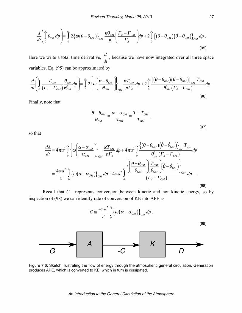
inspection of (98) we can identify rate of conversion of KE into APE as

C ≅4πa2

gω α −αGM( ){ }GM dp

0

ps

∫ .

(99)

Figure 7.6: Sketch illustrating the flow of energy through the atmospheric general circulation. Generation produces APE, which is converted to KE, which in turn is dissipated.

A K

G -C D



The rate of generation or destruction of APE by heating is

G ≅ 4πa2

θ −θGMθGM

⎛

⎝⎜

⎞

⎠⎟ΤGM

θGM

⎛

⎝⎜

⎞

⎠⎟ θ − θGM( )

⎧⎨⎩⎪

⎫⎬⎭⎪GM

Γ d −ΓGM( )dp

0

ps

∫ .

(100)Note that G > 0 if we “heat where it’s hot and cool where it’s cold.” This should sound familiar. A heating field that generates APE destroys entropy.

We can summarize (98) as

dAdt

= C +G .

(101)Similarly, we can show that

dΚdt

= −C − D ,

(102)where K is the globally integrated kinetic energy (e.g., in Joules), and D is the globally integrated dissipation rate. We can also conclude that C is negative from the fact that D > 0 . There must be a net conversion of APE intoKE , in order to supply the KE that is destroyed by dissipation. Because this conversion depletes the APE , the generation of APE must be positive. In other words, energy must flow as shown in Fig. 7.6.

The governing equations for the eddy kinetic energy, zonal kinetic energy, and total kinetic en-ergy

We now present a discussion of the eddy kinetic energy, zonal kinetic energy, and total kinetic energy equations. The derivations of these equations follow methods similar to those used to derive the conservation equation for the potential energy variance, and so will be omitted here for brevity. The derivation is given in a QuickStudy.

We define the eddy kinetic energy per unit mass by

ΚE ≡12

u *( )2 + v *( )2⎡⎣ ⎤⎦ .

(103)It satisfies the following equation:



∂∂tKE

+ 1acosϕ

∂∂ϕ

v[ ]KE + 12v* u*2 + v*2( )⎡⎣ ⎤⎦ + v*φ*⎡⎣ ⎤⎦

⎛⎝⎜

⎞⎠⎟ cosϕ

⎧⎨⎩

⎫⎬⎭

+ ∂∂p

ω[ ]KE + 12

ω * u*2 + v*2( )⎡⎣ ⎤⎦ + ω *φ*⎡⎣ ⎤⎦⎛⎝⎜

⎞⎠⎟

+u*v*⎡⎣ ⎤⎦a

∂ u[ ]∂ϕ

+v*v*⎡⎣ ⎤⎦a

∂ v[ ]∂ϕ

+ u*ω *⎡⎣ ⎤⎦∂ u[ ]∂p

+ v*ω *⎡⎣ ⎤⎦∂ v[ ]∂p

= − u[ ] u*v*⎡⎣ ⎤⎦ + u*u*⎡⎣ ⎤⎦ v[ ]( ) tanϕa− ω *α *⎡⎣ ⎤⎦

+ u*g ∂Fu*

∂p⎡

⎣⎢

⎤

⎦⎥ + v*g ∂Fv

*

∂p⎡

⎣⎢

⎤

⎦⎥ .

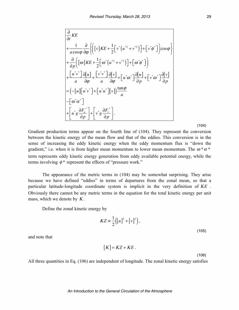
(104)Gradient production terms appear on the fourth line of (104). They represent the conversion between the kinetic energy of the mean flow and that of the eddies. This conversion is in the sense of increasing the eddy kinetic energy when the eddy momentum flux is “down the gradient,” i.e. when it is from higher mean momentum to lower mean momentum. The ω *α * term represents eddy kinetic energy generation from eddy available potential energy, while the terms involving φ * represent the effects of “pressure work.”

The appearance of the metric terms in (104) may be somewhat surprising. They arise because we have defined “eddies” in terms of departures from the zonal mean, so that a particular latitude-longitude coordinate system is implicit in the very definition of ΚE . Obviously there cannot be any metric terms in the equation for the total kinetic energy per unit mass, which we denote by Κ .

Define the zonal kinetic energy by

ΚZ ≡12

u[ ]2 + v[ ]2( ) ,

(105)and note that

Κ[ ] = ΚZ +ΚE .(106)

All three quantities in Eq. (106) are independent of longitude. The zonal kinetic energy satisfies



∂∂tKZ

+ 1acosϕ

∂∂ϕ

v[ ]KZ + u[ ] v*u*⎡⎣ ⎤⎦ + v[ ] v*v*⎡⎣ ⎤⎦ + v[ ] φ[ ]( )cosϕ{ }+ ∂∂p

ω[ ]KZ + u[ ] ω *u*⎡⎣ ⎤⎦ + v[ ] ω *v*⎡⎣ ⎤⎦ + ω[ ] φ[ ]( )

=v*u*⎡⎣ ⎤⎦a

∂ u[ ]∂ϕ

+v*v*⎡⎣ ⎤⎦a

∂ v[ ]∂ϕ

+ ω *u*⎡⎣ ⎤⎦∂ u[ ]∂p

+ ω *v*⎡⎣ ⎤⎦∂ v[ ]∂p

+ u[ ] v*u*⎡⎣ ⎤⎦ − v[ ] u*u*⎡⎣ ⎤⎦( ) tanϕa− ω[ ] α[ ]

+ u[ ]g ∂ Fu[ ]∂p

+ v[ ]∂ Fv[ ]∂p

.

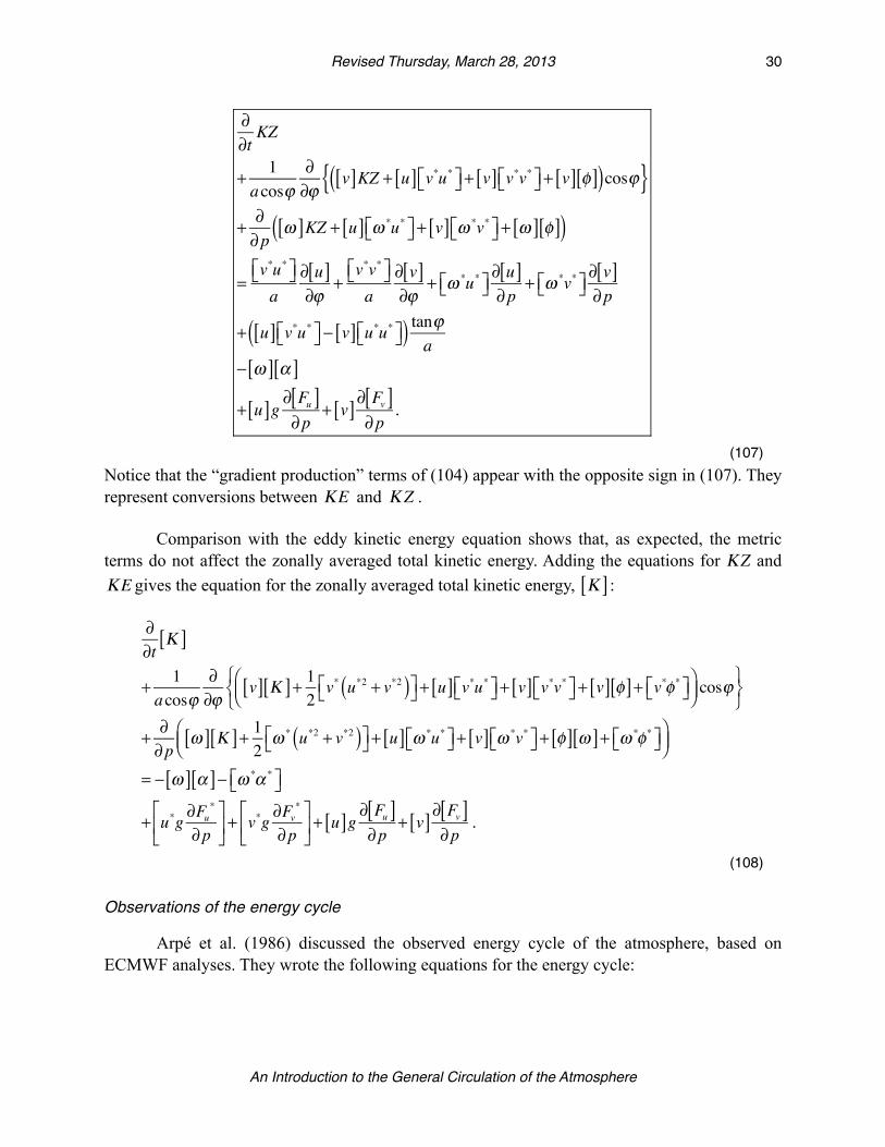
(107)Notice that the “gradient production” terms of (104) appear with the opposite sign in (107). They represent conversions between ΚE and ΚZ .

Comparison with the eddy kinetic energy equation shows that, as expected, the metric terms do not affect the zonally averaged total kinetic energy. Adding the equations for ΚZ and ΚE gives the equation for the zonally averaged total kinetic energy, Κ[ ] :

∂∂t

Κ[ ]

+ 1acosϕ

∂∂ϕ

v[ ] Κ[ ]+ 12 v* u*2 + v*2( )⎡⎣ ⎤⎦ + u[ ] v*u*⎡⎣ ⎤⎦ + v[ ] v*v*⎡⎣ ⎤⎦ + v[ ] φ[ ]+ v*φ*⎡⎣ ⎤⎦⎛⎝⎜

⎞⎠⎟ cosϕ

⎧⎨⎩

⎫⎬⎭

+ ∂∂p

ω[ ] Κ[ ]+ 12 ω * u*2 + v*2( )⎡⎣ ⎤⎦ + u[ ] ω *u*⎡⎣ ⎤⎦ + v[ ] ω *v*⎡⎣ ⎤⎦ + φ[ ] ω[ ]+ ω *φ*⎡⎣ ⎤⎦⎛⎝⎜

⎞⎠⎟

= − ω[ ] α[ ]− ω *α *⎡⎣ ⎤⎦

+ u*g ∂Fu*

∂p⎡

⎣⎢

⎤

⎦⎥ + v*g ∂Fv

*

∂p⎡

⎣⎢

⎤

⎦⎥ + u[ ]g ∂ Fu[ ]

∂p+ v[ ]∂ Fv[ ]

∂p.

(108)

Observations of the energy cycle

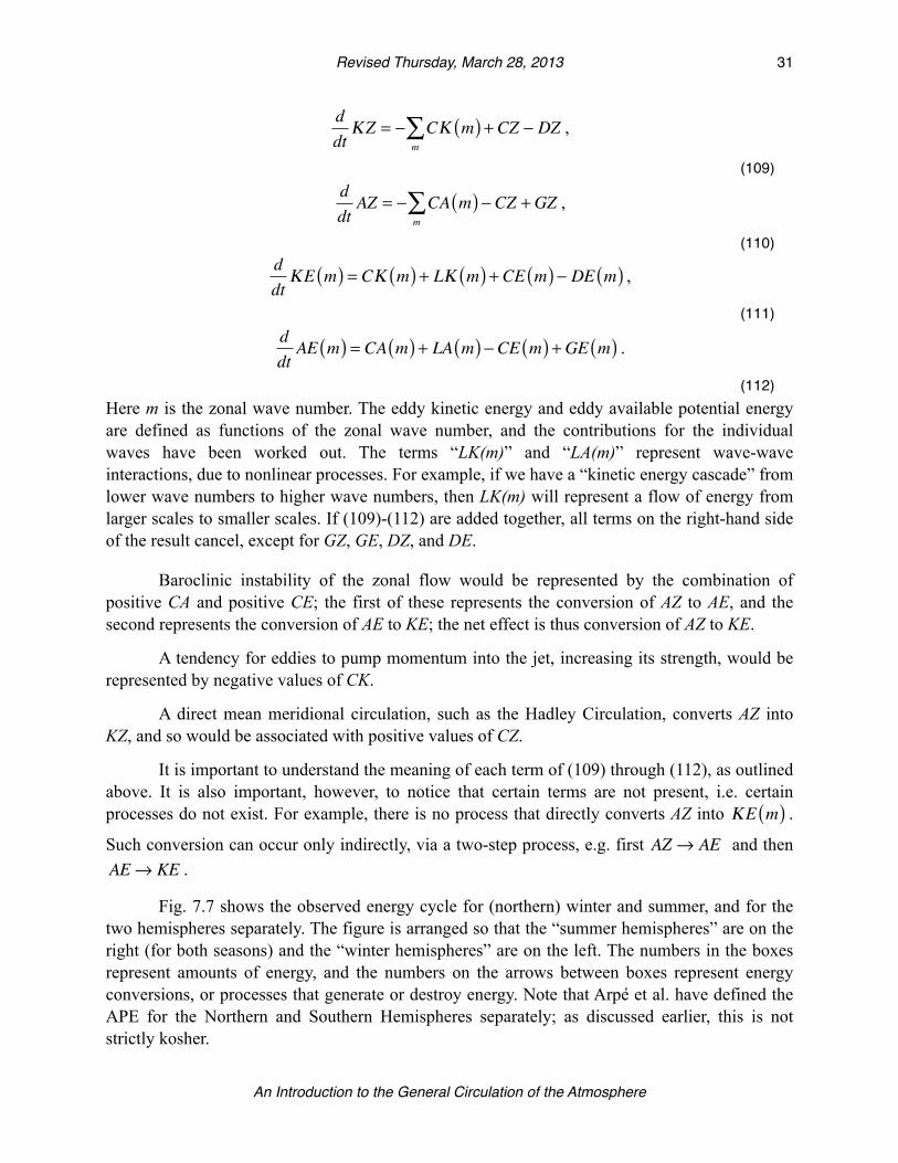
Arpé et al. (1986) discussed the observed energy cycle of the atmosphere, based on ECMWF analyses. They wrote the following equations for the energy cycle:



ddt

ΚZ = − CΚ m( ) + CZ − DZm∑ ,

(109)ddtAZ = − CA m( ) − CZ +GZ

m∑ ,

(110)ddt

ΚE m( ) = CΚ m( ) + LΚ m( ) + CE m( ) − DE m( ) ,

(111)ddtAE m( ) = CA m( ) + LA m( ) − CE m( ) +GE m( ) .

(112)Here m is the zonal wave number. The eddy kinetic energy and eddy available potential energy are defined as functions of the zonal wave number, and the contributions for the individual waves have been worked out. The terms “LK(m)” and “LA(m)” represent wave-wave interactions, due to nonlinear processes. For example, if we have a “kinetic energy cascade” from lower wave numbers to higher wave numbers, then LK(m) will represent a flow of energy from larger scales to smaller scales. If (109)-(112) are added together, all terms on the right-hand side of the result cancel, except for GZ, GE, DZ, and DE.

Baroclinic instability of the zonal flow would be represented by the combination of positive CA and positive CE; the first of these represents the conversion of AZ to AE, and the second represents the conversion of AE to KE; the net effect is thus conversion of AZ to KE.

A tendency for eddies to pump momentum into the jet, increasing its strength, would be represented by negative values of CK.

A direct mean meridional circulation, such as the Hadley Circulation, converts AZ into KZ, and so would be associated with positive values of CZ.

It is important to understand the meaning of each term of (109) through (112), as outlined above. It is also important, however, to notice that certain terms are not present, i.e. certain processes do not exist. For example, there is no process that directly converts AZ into ΚE m( ) .

Such conversion can occur only indirectly, via a two-step process, e.g. first AZ→ AE and then AE→ KE .

Fig. 7.7 shows the observed energy cycle for (northern) winter and summer, and for the two hemispheres separately. The figure is arranged so that the “summer hemispheres” are on the right (for both seasons) and the “winter hemispheres” are on the left. The numbers in the boxes represent amounts of energy, and the numbers on the arrows between boxes represent energy conversions, or processes that generate or destroy energy. Note that Arpé et al. have defined the APE for the Northern and Southern Hemispheres separately; as discussed earlier, this is not strictly kosher.



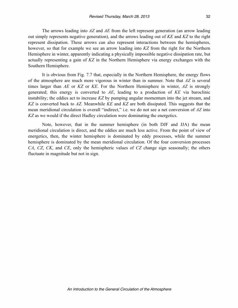
The arrows leading into AZ and AE from the left represent generation (an arrow leading out simply represents negative generation), and the arrows leading out of KE and KZ to the right represent dissipation. These arrows can also represent interactions between the hemispheres, however, so that for example we see an arrow leading into KZ from the right for the Northern Hemisphere in winter, apparently indicating a physically impossible negative dissipation rate, but actually representing a gain of KZ in the Northern Hemisphere via energy exchanges with the Southern Hemisphere.

It is obvious from Fig. 7.7 that, especially in the Northern Hemisphere, the energy flows of the atmosphere are much more vigorous in winter than in summer. Note that AZ is several times larger than AE or KZ or KE. For the Northern Hemisphere in winter, AZ is strongly generated; this energy is converted to AE, leading to a production of KE via baroclinic instability; the eddies act to increase KZ by pumping angular momentum into the jet stream, and KZ is converted back to AZ. Meanwhile KE and KZ are both dissipated. This suggests that the mean meridional circulation is overall “indirect,” i.e. we do not see a net conversion of AZ into KZ as we would if the direct Hadley circulation were dominating the energetics.

Note, however, that in the summer hemisphere (in both DJF and JJA) the mean meridional circulation is direct, and the eddies are much less active. From the point of view of energetics, then, the winter hemisphere is dominated by eddy processes, while the summer hemisphere is dominated by the mean meridional circulation. Of the four conversion processes CA, CZ, CK, and CE, only the hemispheric values of CZ change sign seasonally; the others fluctuate in magnitude but not in sign.



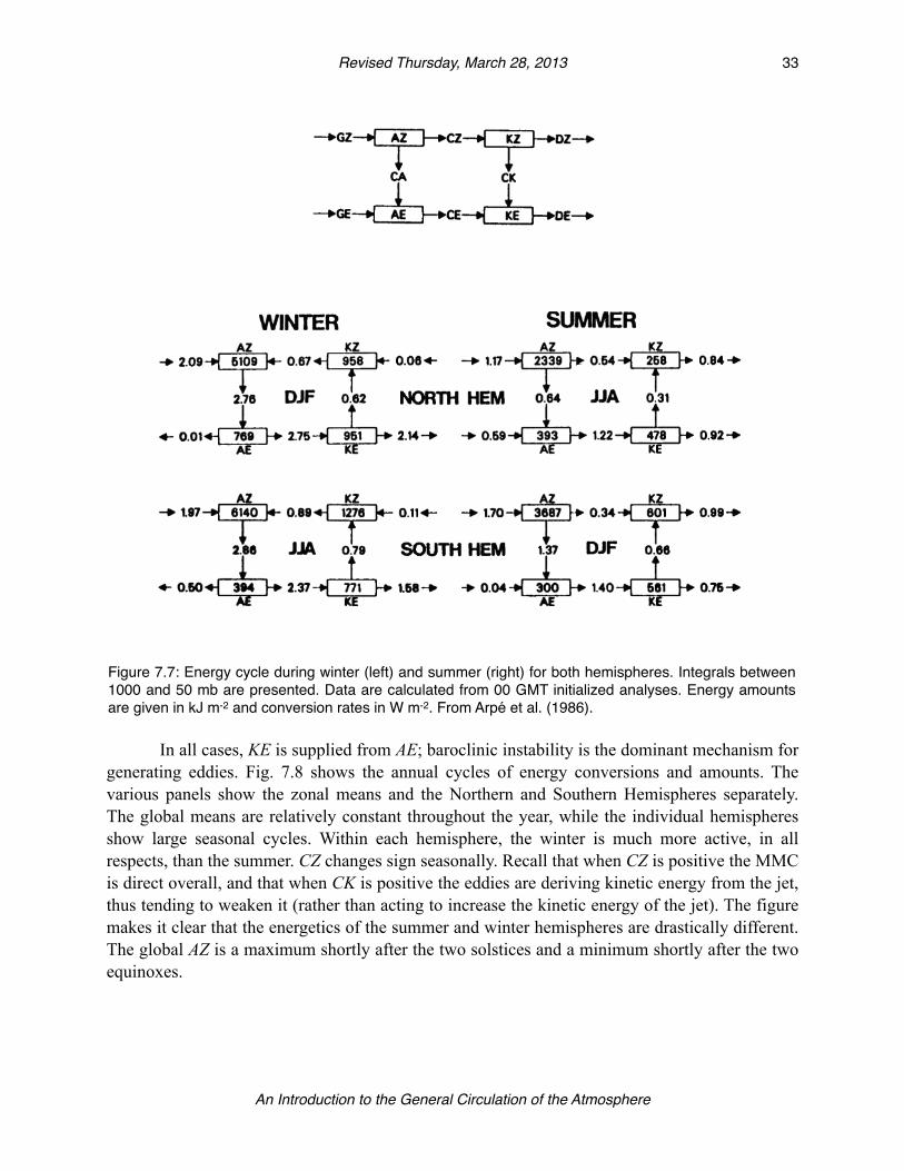
In all cases, KE is supplied from AE; baroclinic instability is the dominant mechanism for generating eddies. Fig. 7.8 shows the annual cycles of energy conversions and amounts. The various panels show the zonal means and the Northern and Southern Hemispheres separately. The global means are relatively constant throughout the year, while the individual hemispheres show large seasonal cycles. Within each hemisphere, the winter is much more active, in all respects, than the summer. CZ changes sign seasonally. Recall that when CZ is positive the MMC is direct overall, and that when CK is positive the eddies are deriving kinetic energy from the jet, thus tending to weaken it (rather than acting to increase the kinetic energy of the jet). The figure makes it clear that the energetics of the summer and winter hemispheres are drastically different. The global AZ is a maximum shortly after the two solstices and a minimum shortly after the two equinoxes.

Figure 7.7: Energy cycle during winter (left) and summer (right) for both hemispheres. Integrals between 1000 and 50 mb are presented. Data are calculated from 00 GMT initialized analyses. Energy amounts are given in kJ m-2 and conversion rates in W m-2. From Arpé et al. (1986).



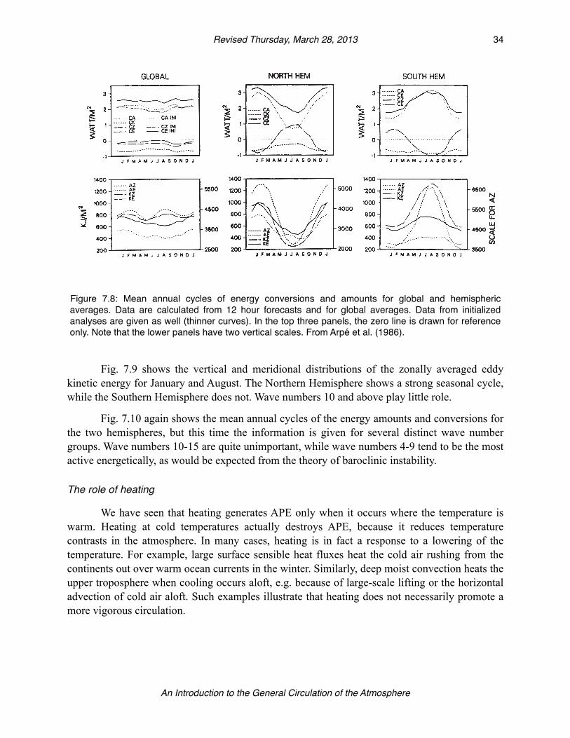
Fig. 7.9 shows the vertical and meridional distributions of the zonally averaged eddy kinetic energy for January and August. The Northern Hemisphere shows a strong seasonal cycle, while the Southern Hemisphere does not. Wave numbers 10 and above play little role.

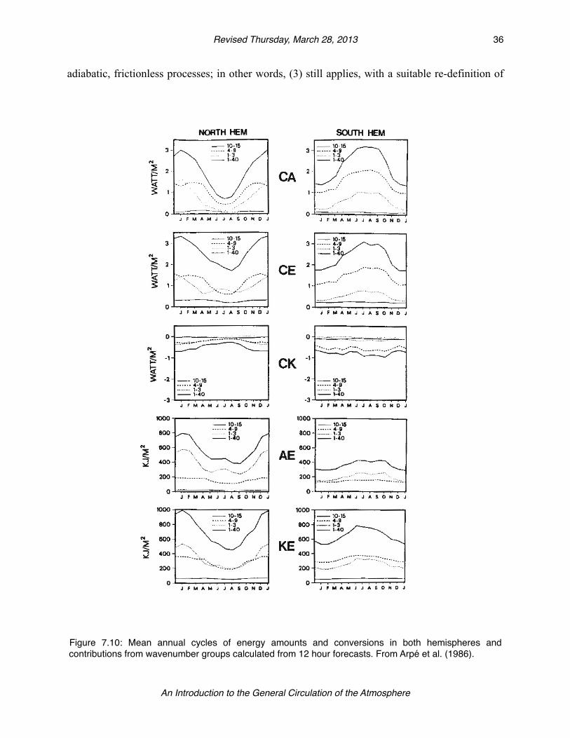
Fig. 7.10 again shows the mean annual cycles of the energy amounts and conversions for the two hemispheres, but this time the information is given for several distinct wave number groups. Wave numbers 10-15 are quite unimportant, while wave numbers 4-9 tend to be the most active energetically, as would be expected from the theory of baroclinic instability.

The role of heating

We have seen that heating generates APE only when it occurs where the temperature is warm. Heating at cold temperatures actually destroys APE, because it reduces temperature contrasts in the atmosphere. In many cases, heating is in fact a response to a lowering of the temperature. For example, large surface sensible heat fluxes heat the cold air rushing from the continents out over warm ocean currents in the winter. Similarly, deep moist convection heats the upper troposphere when cooling occurs aloft, e.g. because of large-scale lifting or the horizontal advection of cold air aloft. Such examples illustrate that heating does not necessarily promote a more vigorous circulation.

Figure 7.8: Mean annual cycles of energy conversions and amounts for global and hemispheric averages. Data are calculated from 12 hour forecasts and for global averages. Data from initialized analyses are given as well (thinner curves). In the top three panels, the zero line is drawn for reference only. Note that the lower panels have two vertical scales. From Arpé et al. (1986).



Moist available energy

Lorenz (1978, 1979) extended the concept of available potential energy by allowing moist adiabatic processes to occur during the transition to the A-state. In order to do this, he had to replace the dry enthalpy,cpΤ , by a moist enthalpy, which is approximately given by

h ≅ cpΤ − Ll .

(113)As before, it can be shown that the integral of the moist enthalpy over the whole atmosphere, added to the integral of the kinetic energy over the whole atmosphere, is invariant under moist

Figure 7.9: Vertical and meridional distribution of zonal mean eddy kinetic energy KE together with contributions by wavenumber groups to vertical integrals in January and August. Units in the cross-sections are J (m2Pa)-1 = 100 kJ (m2Bar)-1. From Arpé et al. (1986).



adiabatic, frictionless processes; in other words, (3) still applies, with a suitable re-definition of

Figure 7.10: Mean annual cycles of energy amounts and conversions in both hemispheres and contributions from wavenumber groups calculated from 12 hour forecasts. From Arpé et al. (1986).



H , based on (113).

With the conventional “dry available energy,” which we have been calling the available potential energy up to now, processes that involve phase changes can either create or destroy A . In the case of moist available energy, phase changes have no direct effect, but the surface fluxes of moisture due to evaporation and precipitation can be quite important (Lorenz, 1979). The concept of moist available energy has not been developed much up to now. It is ripe for further investigation.

Summary

We defined the available potential energy and the gross static stability, and studied the generation and conversion of available potential energy. Finally we presented observations of the atmospheric energy cycle.

The observations of Arpé et al. remind us again of the wide range of eddy scales that are simultaneously at work in the general circulation the atmosphere. All of these eddies undergo their life cycles in the presence of the same mean meridional circulation. The complicated nonlinear interactions among the eddies are the subject of a later chapter, in which we view the general circulation as a kind of large-scale turbulence.



Problems1. Prove that the mass-integrated potential energy of the entire atmosphere is lower in the A-

state than in the given state.

2. Derive (17).

3. Prove that

pκθ dp0

ps

∫ =1

1+κp1+κ dθ

0

∞

∫ .

(114)Note that on the right-hand side the lower limit of integration is zero. This result is used to derive (10) from (9).

4. Prove that S ≥ 0 , where S is given by (30). State any assumptions.

5. The shallow water equations are:

∂h∂t

+ ∇ ⋅ hV( ) = 0 ,

(115)∂V∂t

+ ζ + f( )k × V +∇ Κ + g h + hS( )⎡⎣ ⎤⎦ = 0 ,

(116)

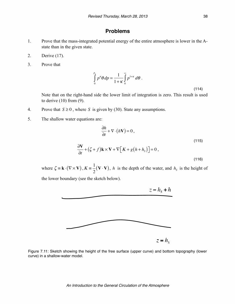
where ζ ≡ k ⋅ ∇ × V( ) ,Κ ≡12V ⋅V( ) , h is the depth of the water, and hS is the height of

the lower boundary (see the sketch below).

Figure 7.11: Sketch showing the height of the free surface (upper curve) and bottom topography (lower curve) in a shallow-water model.



a) Show that the available potential energy of the system, per unit area, is

A =12g H 2 − H 2( ) , where H ≡ h + hS , and the bar represents an average over the whole

domain.

b) Prove that

ddt

A + hΚ( ) = 0 .

(117)6.

a) For the example given in the discussion beginning with Eq. (34), calculate the variance of θ for both the given state and the A-state, and demonstrate that the two variances are equal.

b) Continuing the example, assume that

Fθ = −Da∂θ∂ϕ

,

(118)where D is a positive diffusion coefficient. Derive expressions for the time rates of change of the APE and the potential temperature variance, valid at the instant when θ ϕ( )

satisfies Eq. (34).

c) Suppose that we add a “heating” term to (47), so that it becomes

∂θ∂t

= −1

acosϕ∂∂ϕ

Fθ cosϕ( ) +Q ϕ( ) .

(119)Continue to use the form of Fθ given in part b) above. Find the form of Q ϕ( ) needed to

maintain a steady state. Plot Q ϕ( ) . Find the global mean of Q ϕ( ) . Find the covariance

of Q ϕ( ) and θ . Discuss.

7. Suppose that

ddtAZ = GZ −

AZτ Z

≅ 0,

ddt

ΚE = CE −ΚEτ E

≅ 0,

(120)



Estimate the values of the time scales τ Z and τ E , by using the numerical values given in

Fig. 7.7. Compare GZ and CE with the actual rates of change of AZ and KE as shown in Fig. 7.8.



7. The Energy Cycle - Colorado State Universitykiwi.atmos.colostate.edu/group/dave/at605pdf/Chapter_7.pdf · negative quantity A=H gs ... concept of available potential energy, ...

Documents