7 Statistical Intervals Based on a Single Sample

Welcome message from author
This document is posted to help you gain knowledge. Please leave a comment to let me know what you think about it! Share it to your friends and learn new things together.
Transcript

7Statistical Intervals Based on a Single
Sample

7.1 Basic Properties of Confidence Intervals

3
Basic Properties of Confidence Intervals
The basic concepts and properties of confidence intervals (CIs) are most easily introduced by first focusing on a simple and problem situation.
Suppose that the parameter of interest is a population mean and that
1. The population distribution is normal
2. The value of the population standard deviation is known

4
Basic Properties of Confidence Intervals
Irrespective of the sample size n, the sample mean X is normally distributed with expected value and standard deviation
Standardizing X by first subtracting its expected valueand then dividing by its standard deviation yields thestandard normal variable
(7.1)

5
Basic Properties of Confidence Intervals
Because the area under the standard normal curve between –1.96 and 1.96 is .95,
The equivalence of each set of inequalities to the original set implies that
(7.2)
(7.3)
6
Basic Properties of Confidence Intervals
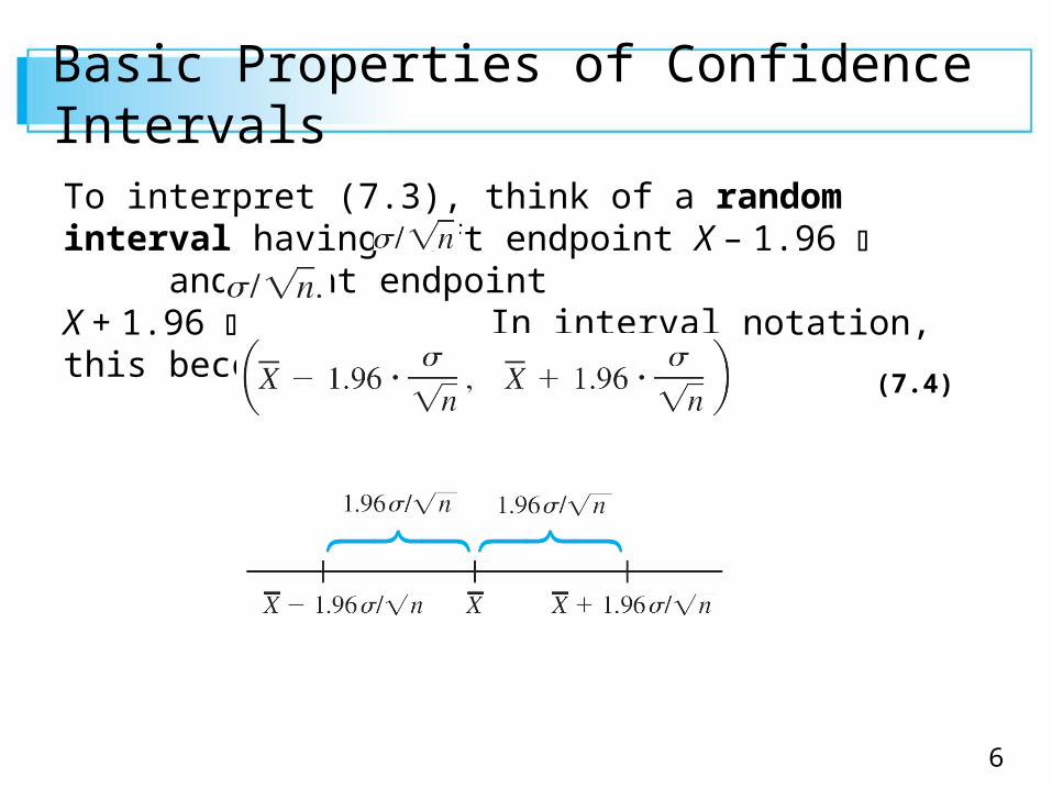
To interpret (7.3), think of a random interval having left endpoint X – 1.96 and right endpointX + 1.96 In interval notation, this becomes
(7.4)
7
Basic Properties of Confidence Intervals
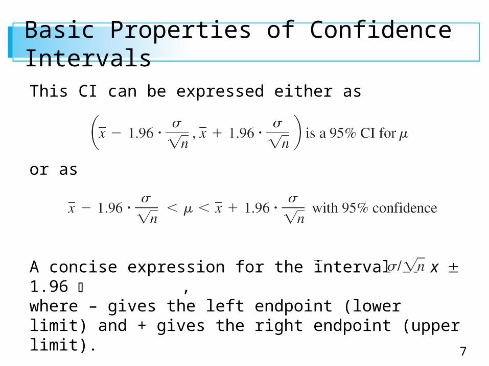
This CI can be expressed either as
or as
A concise expression for the interval is x 1.96 ,where – gives the left endpoint (lower limit) and + gives the right endpoint (upper limit).

8
Interpreting a Confidence IntervalWith 95% confidence, we can say
that µ should be within roughly
1.96 standard deviations
(1.96/√n) from our sample mean
.
• In 95% of all possible samples
of this size n, µ will indeed fall
in our confidence interval.
• In only 5% of samples would
be farther from µ.
n
x
x
9
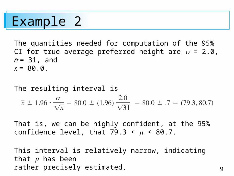
Example 2
The quantities needed for computation of the 95% CI for true average preferred height are = 2.0, n = 31, and x = 80.0.
The resulting interval is
That is, we can be highly confident, at the 95% confidence level, that 79.3 < < 80.7.
This interval is relatively narrow, indicating that has beenrather precisely estimated.
10
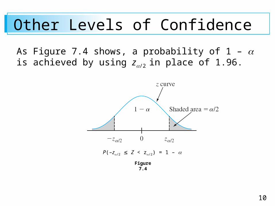
Other Levels of Confidence
As Figure 7.4 shows, a probability of 1 – is achieved by using z/2 in place of 1.96.
Figure 7.4
P(–z/2 Z < z/2) = 1 –

11
Other Levels of Confidence
DefinitionA 100(1 – )% confidence interval for the mean of a normal population when the value of is known is given by
or, equivalently, by
The formula (7.5) for the CI can also be expressed in words as point estimate of (z critical value) (standard error of the mean).
(7.5)
12
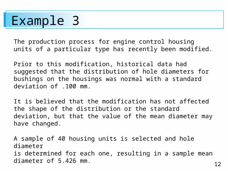
Example 3
The production process for engine control housing units of a particular type has recently been modified.
Prior to this modification, historical data had suggested that the distribution of hole diameters for bushings on the housings was normal with a standard deviation of .100 mm.
It is believed that the modification has not affected the shape of the distribution or the standard deviation, but that the value of the mean diameter may have changed.
A sample of 40 housing units is selected and hole diameteris determined for each one, resulting in a sample mean diameter of 5.426 mm.

13
Example 3
Let’s calculate a confidence interval for true average hole diameter using a confidence level of 90%.
This requires that 100(1 – ) = 90, from which = .10 andz/2 = z.05 = 1.645 (corresponding to a cumulative z-curve area of .9500). The desired interval is then
With a reasonably high degree of confidence, we can say that 5.400 < < 5.452.
This interval is rather narrow because of the small amount of variability in hole diameter ( = .100).
cont’d
14
User chooses the confidence interval
We want
High confidence
Small confidence interval
The confidence interval gets narrower when
z gets smaller
σ is smaller
n is larger
Properties of Confidence Intervals
15
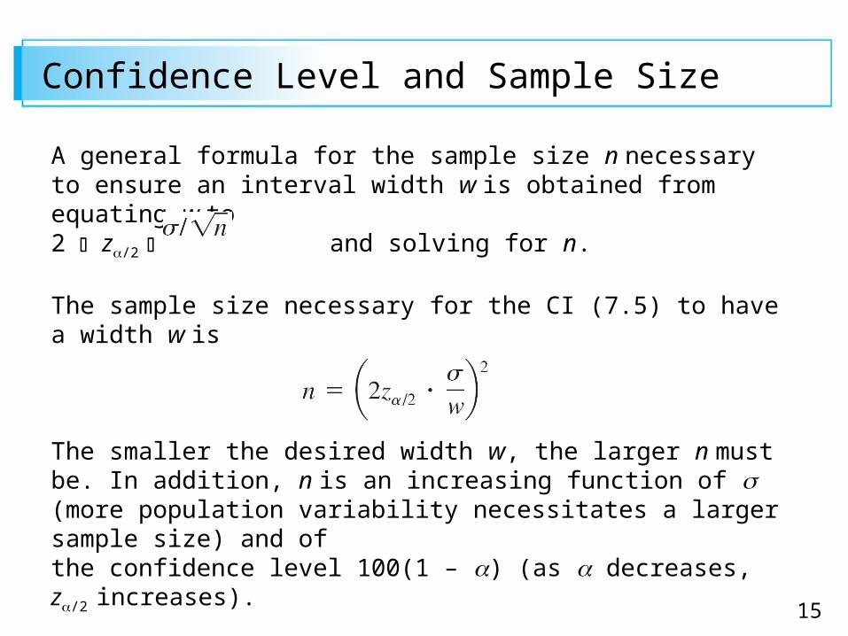
Confidence Level and Sample Size
A general formula for the sample size n necessary to ensure an interval width w is obtained from equating w to2 z/2 and solving for n.
The sample size necessary for the CI (7.5) to have a width w is
The smaller the desired width w, the larger n must be. In addition, n is an increasing function of (more population variability necessitates a larger sample size) and ofthe confidence level 100(1 – ) (as decreases, z/2
increases).
16
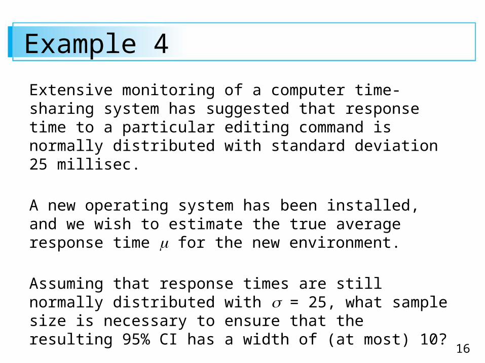
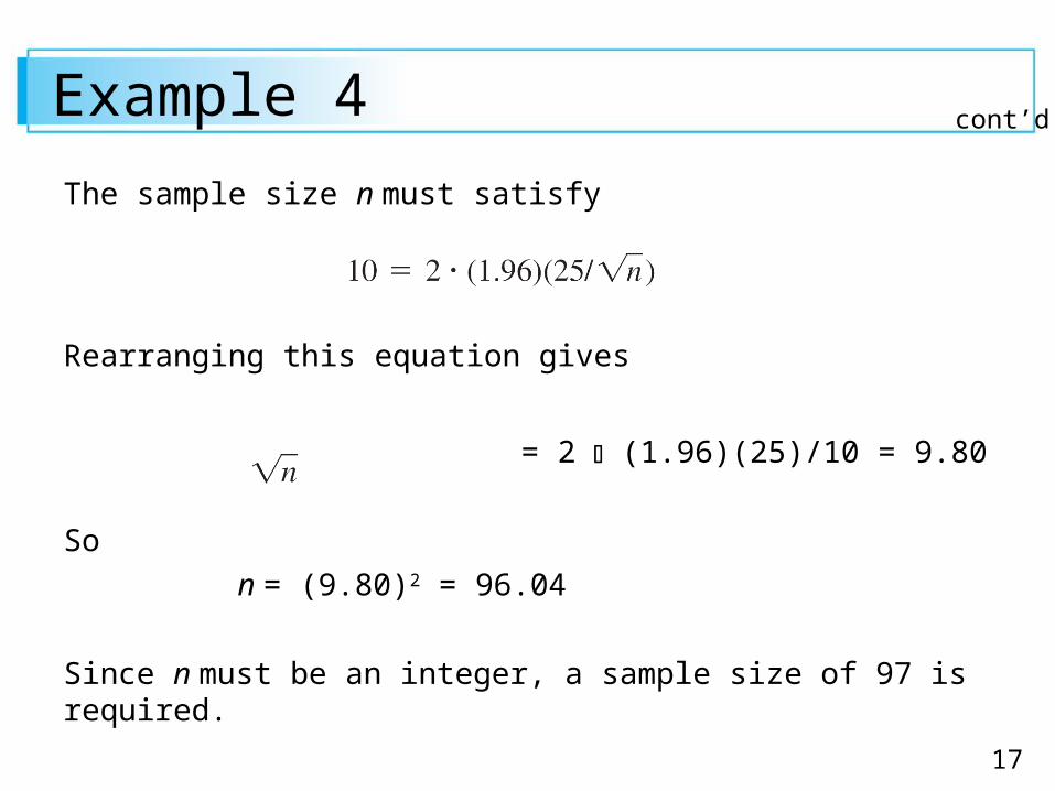
Example 4
Extensive monitoring of a computer time-sharing system has suggested that response time to a particular editing command is normally distributed with standard deviation 25 millisec.
A new operating system has been installed, and we wish to estimate the true average response time for the new environment.
Assuming that response times are still normally distributed with = 25, what sample size is necessary to ensure that the resulting 95% CI has a width of (at most) 10?
17
Example 4
The sample size n must satisfy
Rearranging this equation gives
= 2 (1.96)(25)/10 = 9.80
So
n = (9.80)2 = 96.04
Since n must be an integer, a sample size of 97 is required.
cont’d
18
7.2Large-Sample Confidence
Intervals for a Population Mean and Proportion
19
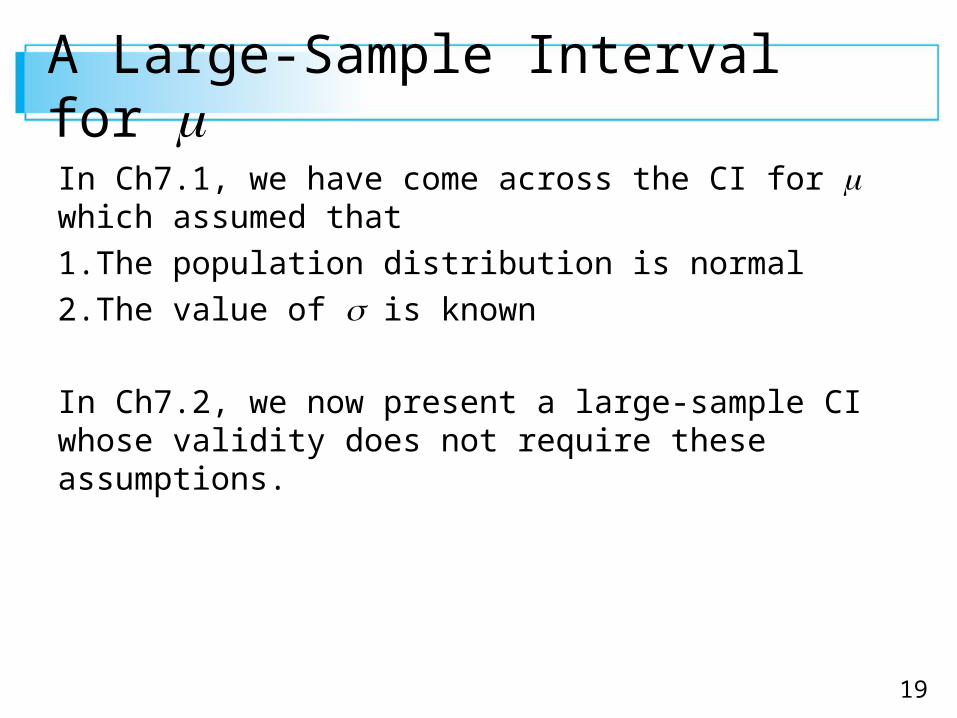
A Large-Sample Interval for In Ch7.1, we have come across the CI for which assumed that
1.The population distribution is normal
2.The value of is known
In Ch7.2, we now present a large-sample CI whose validity does not require these assumptions.

20
A Large-Sample Interval for Let X1, X2, . . . , Xn be a random sample from a population having a mean and standard deviation . Provided that n is large, the Central Limit Theorem (CLT) implies that has approximately a normal distribution whatever the nature of the population distribution.
It then follows that has approximately a standard normal distribution, so that
21
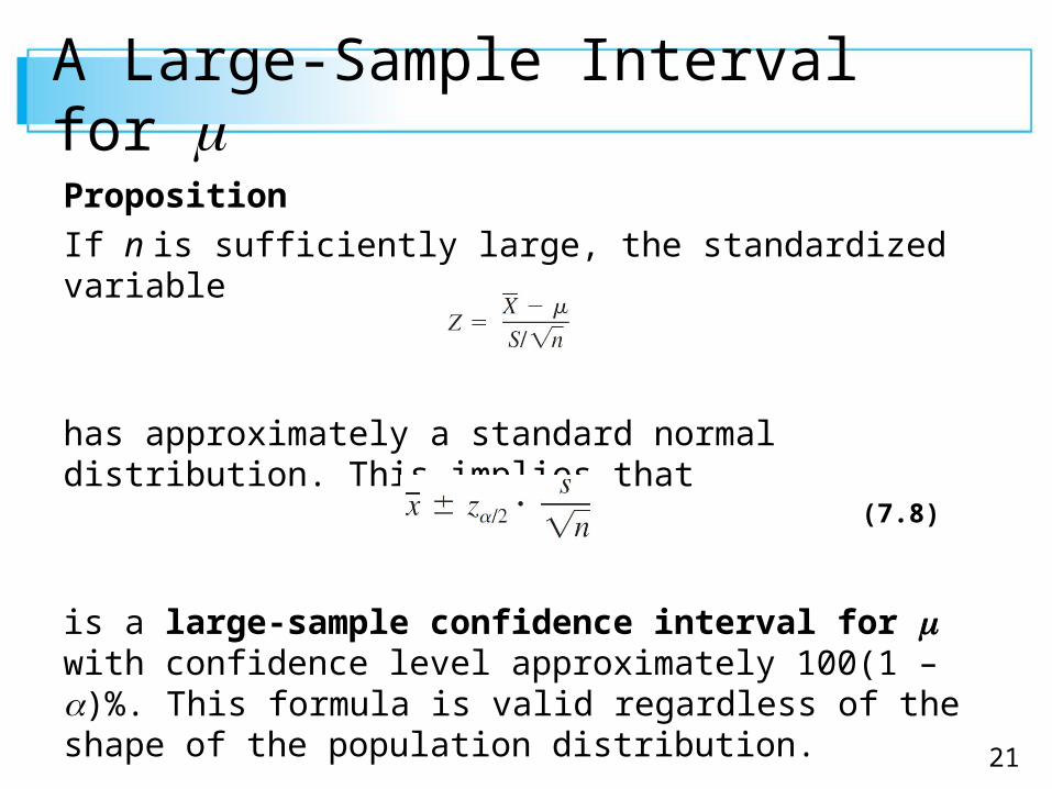
A Large-Sample Interval for Proposition
If n is sufficiently large, the standardized variable
has approximately a standard normal distribution. This implies that
is a large-sample confidence interval for with confidence level approximately 100(1 – )%. This formula is valid regardless of the shape of the population distribution.
(7.8)
22
A Large-Sample Interval for Generally speaking, n > 40 will be sufficient to justify the use of this interval.
This is somewhat more conservative than the rule of thumb for the CLT because of the additional variability introduced by using S in place of .

23
Example 6
Haven’t you always wanted to own a Porsche? The author thought maybe he could afford a Boxster, the cheapest model. So he went to www.cars.com on Nov. 18, 2009, and found a total of 1113 such cars listed.
Asking prices ranged from $3499 to $130,000 (the latter price was one of only two exceeding $70,000). The prices depressed him, so he focused instead on odometer readings (miles).
24
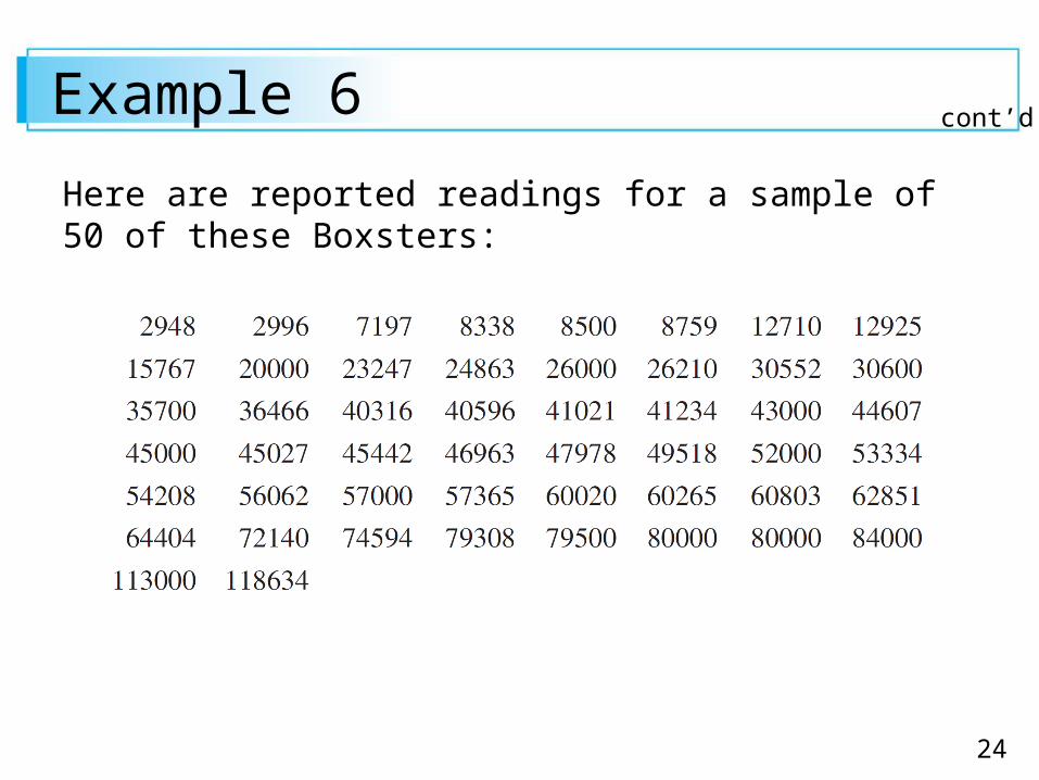
Example 6
Here are reported readings for a sample of 50 of these Boxsters:
cont’d
25
Example 6
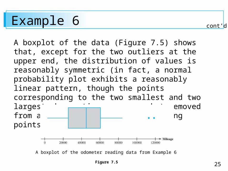
A boxplot of the data (Figure 7.5) shows that, except for the two outliers at the upper end, the distribution of values is reasonably symmetric (in fact, a normal probability plot exhibits a reasonably linear pattern, though the points corresponding to the two smallest and two largest observations are somewhat removed from a line fit through the remaining points).
A boxplot of the odometer reading data from Example 6
Figure 7.5
cont’d
26
Example 6
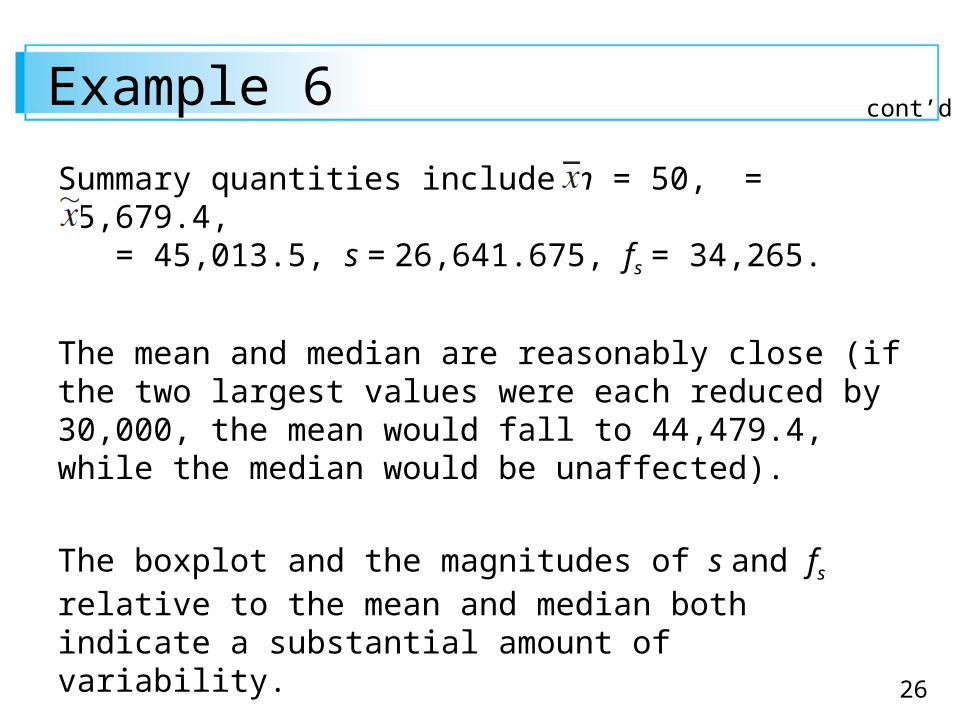
Summary quantities include n = 50, = 45,679.4, = 45,013.5, s = 26,641.675, fs = 34,265.
The mean and median are reasonably close (if the two largest values were each reduced by 30,000, the mean would fall to 44,479.4, while the median would be unaffected).
The boxplot and the magnitudes of s and fs relative to the mean and median both indicate a substantial amount of variability.
cont’d

27
Example 6
A confidence level of about 95% requires z.025 = 1.96, and the interval is
45,679.4 (1.96) = 45,679.4 7384.7
= (38,294.7, 53,064.1)
That is, 38,294.7 < < 53,064.1 with 95% confidence. This interval is rather wide because a sample size of 50, even though large by our rule of thumb, is not large enough to overcome the substantial variability in the sample. We do not have a very precise estimate of the population mean odometer reading.
cont’d

28
One-Sided Confidence Intervals (Confidence Bounds)
Starting with P(–1.645 < Z) .95 and manipulating the inequality results in the upper confidence bound. A similar argument gives a one-sided bound associated with any other confidence level.
Proposition
A large-sample upper confidence bound for is
and a large-sample lower confidence bound for is
29
7.3 Intervals Based on a Normal Population Distribution
30
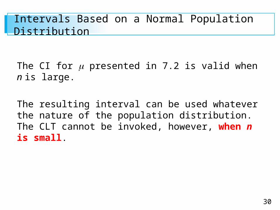
Intervals Based on a Normal Population Distribution
The CI for presented in 7.2 is valid when n is large.
The resulting interval can be used whatever the nature of the population distribution. The CLT cannot be invoked, however, when n is small.

31
Intervals Based on a Normal Population Distribution
The result on which inferences are based introduces a new family of probability distributions called t distributions.
Theorem
When is the mean of a random sample of size n from a normal distribution with mean , the rv
has a probability distribution called a t distribution with n – 1 degrees of freedom (df).
(7.13)

32
Properties of t Distributions
Properties of t Distributions
Let t denote the t distribution with df.1. Each t curve is bell-shaped and centered at 0.
2. Each t curve is more spread out than the standard normal (z) curve.
3. As increases, the spread of the corresponding t curve decreases.
4. As , the sequence of t curves approaches the standard normal curve (so the z curve is often called the t curve with df = ).

33
Properties of t Distributions
Figure 7.7 illustrates several of these properties for selected values of .
Figure 7.7
t and z curves

34
Properties of t Distributions
Notation
Let t, = the number on the measurement axis for which the area under the t curve with df to the right of t, is ; t, is called a t critical value.
For example, t.05,6 is the t critical value that captures an upper-tail area of .05 under the t curve with 6 df. The general notation is illustrated in Figure 7.8.
Figure 7.8
Illustration of a t critical value
35
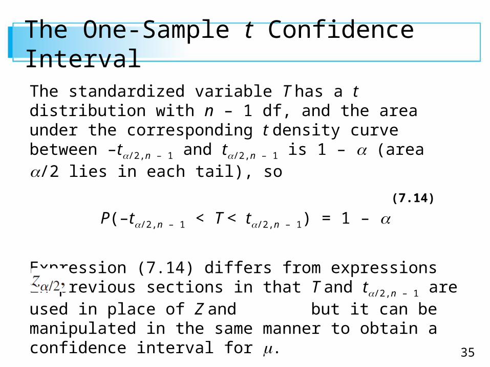
The One-Sample t Confidence Interval
The standardized variable T has a t distribution with n – 1 df, and the area under the corresponding t density curve between –t/2,n – 1 and t/2,n – 1 is 1 – (area /2 lies in each tail), so
P(–t/2,n – 1 < T < t/2,n – 1) = 1 –
Expression (7.14) differs from expressions in previous sections in that T and t/2,n – 1 are used in place of Z and
but it can be manipulated in the same manner to obtain a confidence interval for .
(7.14)

36
The One-Sample t Confidence Interval
Proposition
Let and s be the sample mean and sample standard deviation computed from the results of a random sample from a normal population with mean . Then a 100(1 – )% confidence interval for is
or, more compactly
(7.15)
37
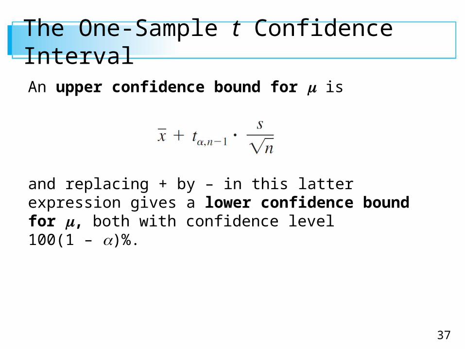
The One-Sample t Confidence Interval
An upper confidence bound for is
and replacing + by – in this latter expression gives a lower confidence bound for , both with confidence level 100(1 – )%.

38
Example 11
Even as traditional markets for sweetgum lumber have declined, large section solid timbers traditionally used for construction bridges and mats have become increasinglyscarce.
The article “Development of Novel Industrial Laminated Planks from Sweetgum Lumber” (J. of Bridge Engr., 2008: 64–66) described the manufacturing and testing of composite beams designed to add value to low-grade sweetgum lumber.
39
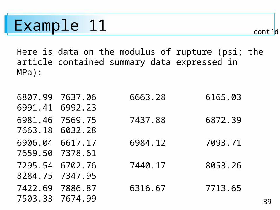
Example 11
Here is data on the modulus of rupture (psi; the article contained summary data expressed in MPa):
6807.99 7637.06 6663.28 6165.03 6991.41 6992.23
6981.46 7569.75 7437.88 6872.39 7663.18 6032.28
6906.04 6617.17 6984.12 7093.71 7659.50 7378.61
7295.54 6702.76 7440.17 8053.26 8284.75 7347.95
7422.69 7886.87 6316.67 7713.65 7503.33 7674.99
cont’d

40
Example 11
Figure 7.9 shows a normal probability plot from the R software.
Figure 7.9
A normal probability plot of the modulus of rupture data
cont’d

41
Example 11
The straightness of the pattern in the plot provides strong support for assuming that the population distribution of MOR is at least approximately normal.
The sample mean and sample standard deviation are 7203.191 and 543.5400, respectively (for anyone bent on doing hand calculation, the computational burden is eased a bit by subtracting 6000 from each x value to obtainyi = xi – 6000; then from which = 1203.191 and sy = sx as given).
cont’d

42
Example 11
Let’s now calculate a confidence interval for true average MOR using a confidence level of 95%. The CI is based on n – 1 = 29 degrees of freedom, so the necessary t critical value is t.025,29 = 2.045. The interval estimate is now
We estimate 7000.253 < < 7406.129 that with 95% confidence.
cont’d

43
Example 11
If we use the same formula on sample after sample, in the long run 95% of the calculated intervals will contain . Since the value of is not available, we don’t know whether the calculated interval is one of the “good” 95% or the “bad” 5%.
Even with the moderately large sample size, our interval is rather wide. This is a consequence of the substantial amount of sample variability in MOR values.
A lower 95% confidence bound would result from retaining only the lower confidence limit (the one with –) and replacing 2.045 with t.05,29 = 1.699.
cont’d
44
Intervals Based on Nonnormal Population Distributions
The one-sample t CI for is robust to small or even moderate departures from normality unless n is quite small.
By this we mean that if a critical value for 95% confidence, for example, is used in calculating the interval, the actual confidence level will be reasonably close to the nominal 95% level.
If, however, n is small and the population distribution is highly nonnormal, then the actual confidence level may be considerably different from the one you think you are using when you obtain a particular critical value from the t table.
45
Intervals Based on Nonnormal Population Distributions
It would certainly be distressing to believe that your confidence level is about 95% when in fact it was really more like 88%!
The bootstrap technique, has been found to be quite successful at estimating parameters in a wide variety of nonnormal situations.
In contrast to the confidence interval, the validity of the prediction and tolerance intervals described in this section is closely tied to the normality assumption.

46
Intervals Based on Nonnormal Population Distributions
These latter intervals should not be used in the absence of compelling evidence for normality.
The excellent reference Statistical Intervals, cited in the bibliography at the end of this chapter, discusses alternative procedures of this sort for various other situations.
Related Documents


![[1] Confidence Intervals. [2] Statistical Estimation sample statistic = parameter estimate = s=s= Example:](https://static.cupdf.com/doc/110x72/55143ca7550346494e8b4718/1-confidence-intervals-2-statistical-estimation-sample-statistic-parameter-estimate-ss-example.jpg)

