§7 Inhomogeneous Equations (31) y +2y - 3y =0, y(0) = 1, y (0) = 0 (32) y - 3y +2y =0, y(0) = 0, y (0) = 1 (33) y - 2y - 8y =0, y(2) = 1, y (2) = 0 (34) y +2y - 5y - 6y =0, y(0) = 1, y (0) = 0, y (0) = 0 (35) y - 4y - 21y =0, y(1) = 0, y (1) = 1 (36) y + y - 3 4 y =0, y(1) = 1, y (1) = 0 (37) y +2y + y =0, y(0) = 1, y (0) = 2 (38) y +6y +9y =0, y(0) = 1, y (0) = 0, y (0) = 0 (39) y +4y +3y =0, y(0) = 3, y (0) = -3, y (0) = 11 (40) y - 8y + 16y =0, y(0) = 0, y (0) = 0, y (0) = 0, y (0) = 0 (41) y + y + y + y =0 (42) y - y + y - y =0 (43) y +4y +6y +4y =0 (44) y +8y + 16y =0 (45) y +5y +4y - 10y =0, y(0) = 1, y (0) = 0, y (0) = 0 §7 Inhomogeneous Equations Discussion: Now that we have learned to solve homogeneous equations, the next topic is inhomogeneous equations. From the discussion in section 5, we know that all we need to find the general solution to an inhomogeneous equation is any one particular solution to the equation along with the general solution to the homogeneous equation. The main method we have to find such a particular solution is called undetermined coefficients . The reason it is called undetermined coefficients is that guessing is not nearly so impressive a name. The basic idea is that if we apply a constant coefficient linear differential operator to the function e rx for any constant r, the result is just Be rx for some constant B. So if we want to solve Ly = Be rx , we should guess the solution is of the form y = Ae rx for some constant A. Having made this guess we plug it into the equation Ly = Be rx and solve for A to find our particular solution. Of course, this guess won’t always work. Then we guess again using somewhat more sophisticated guesses. Undetermined coefficients qualifies as a method rather than just a trick because it is possible to write down a precise procedure for 87

Welcome message from author
This document is posted to help you gain knowledge. Please leave a comment to let me know what you think about it! Share it to your friends and learn new things together.
Transcript

§7 Inhomogeneous Equations
(31) y′′ + 2y′ − 3y = 0, y(0) = 1, y′(0) = 0
(32) y′′ − 3y′ + 2y = 0, y(0) = 0, y′(0) = 1
(33) y′′ − 2y′ − 8y = 0, y(2) = 1, y′(2) = 0
(34) y′′′ + 2y′′ − 5y′ − 6y = 0, y(0) = 1, y′(0) = 0, y′′(0) = 0
(35) y′′ − 4y′ − 21y = 0, y(1) = 0, y′(1) = 1
(36) y′′ + y′ − 34y = 0, y(1) = 1, y′(1) = 0
(37) y′′ + 2y′ + y = 0, y(0) = 1, y′(0) = 2
(38) y′′′ + 6y′′ + 9y′ = 0, y(0) = 1, y′(0) = 0, y′′(0) = 0
(39) y′′′ + 4y′′ + 3y′ = 0, y(0) = 3, y′(0) = −3, y′′(0) = 11
(40) y′′′′ − 8y′′ + 16y = 0, y(0) = 0, y′(0) = 0, y′′(0) = 0, y′′′(0) = 0
(41) y′′′ + y′′ + y′ + y = 0
(42) y′′′ − y′′ + y′ − y = 0
(43) y′′′ + 4y′′ + 6y′ + 4y = 0
(44) y′′′′ + 8y′′ + 16y = 0
(45) y′′′ + 5y′′ + 4y′ − 10y = 0, y(0) = 1, y′(0) = 0, y′′(0) = 0
§7 Inhomogeneous Equations
Discussion: Now that we have learned to solve homogeneous equations, the next topicis inhomogeneous equations. From the discussion in section 5, we know that all we needto find the general solution to an inhomogeneous equation is any one particular solutionto the equation along with the general solution to the homogeneous equation. The mainmethod we have to find such a particular solution is called undetermined coefficients. Thereason it is called undetermined coefficients is that guessing is not nearly so impressive aname. The basic idea is that if we apply a constant coefficient linear differential operatorto the function erx for any constant r, the result is just Berx for some constant B. So ifwe want to solve Ly = Berx, we should guess the solution is of the form y = Aerx for someconstant A. Having made this guess we plug it into the equation Ly = Berx and solve forA to find our particular solution. Of course, this guess won’t always work. Then we guessagain using somewhat more sophisticated guesses. Undetermined coefficients qualifies as amethod rather than just a trick because it is possible to write down a precise procedure for
87

Chapter 2: Linear Constant Coefficient Higher Order Equations
coming up with exactly the right guess. But doing so right now would be more confusingthan helpful. So we will instead deal with the simplest case first and then explain what todo if the obvious guess fails later in the examples.
Paradigm: y′′ + 4y′ + 3y = 4e−2x
STEP 1: Find the general solution to the homogeneous equation, yh(x).
We obtain D2 + 4D + 3 = 0 which has roots −1 and −3. So the general solution to thehomogeneous equation is yh(x) = c1e
−x + c2e−3x.
STEP 2: Guess the form of the particular solution yp(x).
As indicated in the discussion above, a good guess for the form of the particular solutionis yp(x) = Ae−2x.
STEP 3: Plug the guess for the particular solution, yp(x), into the equation and solve forthe undetermined coefficients.
We haveyp(x) = Ae−2x
y′p(x) = −2Ae−2x
y′′p (x) = 4Ae−2x
So plugging into the equation we find
y′′p (x) + 4y′p(x) + 3yp(x) = 4Ae−2x + 4(−2Ae−2x) + 3(Ae−2x)
= (4A− 8A+ 3A)e−2x
= −Ae−2x set= 4e−2x
Solving the last equation we get A = −4 so yp(x) = −4e−2x.
STEP 4: The general solution is now yp(x) + yh(x).
The general solution to the equation is
y(x) = −4e−2x + c1e−x + c2e
−3x
That is a very simple process. We now consider some of the situations where things cango wrong.
88
§7 Inhomogeneous Equations
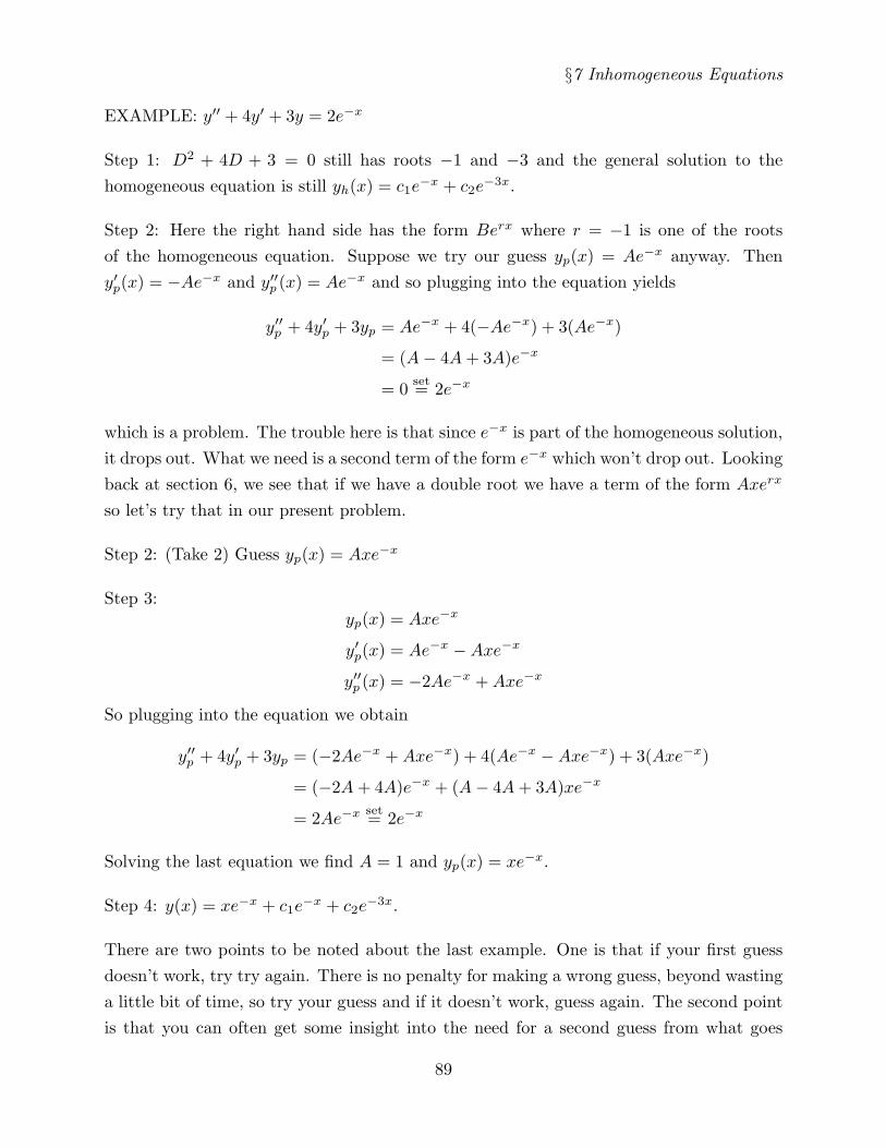
EXAMPLE: y′′ + 4y′ + 3y = 2e−x
Step 1: D2 + 4D + 3 = 0 still has roots −1 and −3 and the general solution to thehomogeneous equation is still yh(x) = c1e
−x + c2e−3x.
Step 2: Here the right hand side has the form Berx where r = −1 is one of the rootsof the homogeneous equation. Suppose we try our guess yp(x) = Ae−x anyway. Theny′p(x) = −Ae−x and y′′p (x) = Ae−x and so plugging into the equation yields
y′′p + 4y′p + 3yp = Ae−x + 4(−Ae−x) + 3(Ae−x)
= (A− 4A+ 3A)e−x
= 0 set= 2e−x
which is a problem. The trouble here is that since e−x is part of the homogeneous solution,it drops out. What we need is a second term of the form e−x which won’t drop out. Lookingback at section 6, we see that if we have a double root we have a term of the form Axerx
so let’s try that in our present problem.
Step 2: (Take 2) Guess yp(x) = Axe−x
Step 3:yp(x) = Axe−x
y′p(x) = Ae−x −Axe−x
y′′p (x) = −2Ae−x +Axe−x
So plugging into the equation we obtain
y′′p + 4y′p + 3yp = (−2Ae−x +Axe−x) + 4(Ae−x −Axe−x) + 3(Axe−x)
= (−2A+ 4A)e−x + (A− 4A+ 3A)xe−x
= 2Ae−x set= 2e−x
Solving the last equation we find A = 1 and yp(x) = xe−x.
Step 4: y(x) = xe−x + c1e−x + c2e
−3x.
There are two points to be noted about the last example. One is that if your first guessdoesn’t work, try try again. There is no penalty for making a wrong guess, beyond wastinga little bit of time, so try your guess and if it doesn’t work, guess again. The second pointis that you can often get some insight into the need for a second guess from what goes
89
Chapter 2: Linear Constant Coefficient Higher Order Equations
wrong with the first guess. In particular from this example, if you end up with an equationof the form 0 = Berx, you probably need to multiply your initial guess by x.
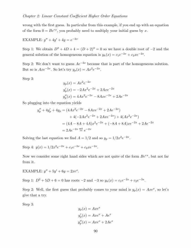
EXAMPLE: y′′ + 4y′ + 4y = e−2x
Step 1: We obtain D2 + 4D + 4 = (D + 2)2 = 0 so we have a double root of −2 and thegeneral solution of the homogeneous equation is yh(x) = c1e
−2x + c2xe−2x.
Step 2: We don’t want to guess Ae−2x because that is part of the homogeneous solution.But so is Axe−2x. So let’s try yp(x) = Ax2e−2x.
Step 3:yp(x) = Ax2e−2x
y′p(x) = −2Ax2e−2x + 2Axe−2x
y′′p (x) = 4Ax2e−2x − 8Axe−2x + 2Ae−2x
So plugging into the equation yields
y′′p + 4y′p + 4yp = (4Ax2e−2x − 8Axe−2x + 2Ae−2x)
+ 4(−2Ax2e−2x + 2Axe−2x) + 4(Ax2e−2x)
= (4A− 8A+ 4A)x2e−2x + (−8A+ 8A)xe−2x + 2Ae−2x
= 2Ae−2x set= e−2x
Solving the last equation we find A = 1/2 and so yp = 1/2x2e−2x.
Step 4: y(x) = 1/2x2e−2x + c1e−2x + c2xe
−2x.
Now we consider some right hand sides which are not quite of the form Berx, but not farfrom it.
EXAMPLE: y′′ + 5y′ + 6y = 2xex.
Step 1: D2 + 5D + 6 = 0 has roots −2 and −3 so yh(x) = c1e−2x + c2e
−3x.
Step 2: Well, the first guess that probably comes to your mind is yp(x) = Axex, so let’sgive that a try.
Step 3:yp(x) = Axex
y′p(x) = Axex +Aex
y′′p (x) = Axex + 2Aex
90

§7 Inhomogeneous Equations
Plugging into our equation we obtain
y′′p + 5y′p + 6yp = (Axex + 2Aex) + 5(Axex +Aex) + 6(Axex)
= (A+ 5A+ 6)xex + (2A+ 5A)ex
= 12Axex + 7Aex set= 2xex
Well that almost worked out. Unfortunately, we got that extra 7Aex term. So how shouldwe get rid of it? But no real harm done, we just have to guess again. And we use thefact that we got an extra 7Aex term to guess that we need a Bex term to go along withour Axex term. That makes sense. Whenever we’ve had an xex term in the past in anysolution we had an ex to go along with it.
Step 2: (Take 2) yp = Axex +Bex.
Step 3: (Take 2)yp(x) = Axex +Bex
y′p(x) = Axex + (A+B)ex
y′′p (x) = Axex + (2A+B)ex
Plugging into our equation we obtain
y′′p + 5y′p + 6yp = (Axex + (2A+B)ex) + 5(Axex + (A+B)ex) + 6(Axex +Bex)
= (A+ 5A+ 6A)xex + (2A+B + 5A+ 5B + 6B)ex
= 12Axex + (7A+ 12B)ex set= 2xex
From the last equation we find 12A = 2 and 7A + 12B = 0, so A = 1/6 and B = −7/72.Hence yp(x) = 1/6xex − 7/72ex.
Step 4: y(x) = 1/6xex − 7/72ex + c1e−2x + c2e
−3x.
Before we consider the next example, we state and prove an easy and useful theorem (thebest kind).
Theorem. Suppose L is a linear operator and Ly = f and Lz = g. Then L(y+z) = f+g.
Proof: This follows immediately from the definition of linearity. L(y + z) = Ly + Lz =f + g.
EXAMPLE: y′′ − 2y′ − 8y = ex − e−x
91
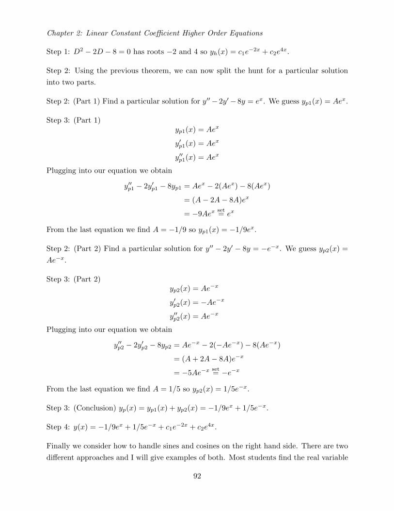
Chapter 2: Linear Constant Coefficient Higher Order Equations
Step 1: D2 − 2D − 8 = 0 has roots −2 and 4 so yh(x) = c1e−2x + c2e
4x.
Step 2: Using the previous theorem, we can now split the hunt for a particular solutioninto two parts.
Step 2: (Part 1) Find a particular solution for y′′− 2y′− 8y = ex. We guess yp1(x) = Aex.
Step 3: (Part 1)yp1(x) = Aex
y′p1(x) = Aex
y′′p1(x) = Aex
Plugging into our equation we obtain
y′′p1 − 2y′p1 − 8yp1 = Aex − 2(Aex)− 8(Aex)
= (A− 2A− 8A)ex
= −9Aex set= ex
From the last equation we find A = −1/9 so yp1(x) = −1/9ex.
Step 2: (Part 2) Find a particular solution for y′′ − 2y′ − 8y = −e−x. We guess yp2(x) =Ae−x.
Step 3: (Part 2)yp2(x) = Ae−x
y′p2(x) = −Ae−x
y′′p2(x) = Ae−x
Plugging into our equation we obtain
y′′p2 − 2y′p2 − 8yp2 = Ae−x − 2(−Ae−x)− 8(Ae−x)
= (A+ 2A− 8A)e−x
= −5Ae−x set= −e−x
From the last equation we find A = 1/5 so yp2(x) = 1/5e−x.
Step 3: (Conclusion) yp(x) = yp1(x) + yp2(x) = −1/9ex + 1/5e−x.
Step 4: y(x) = −1/9ex + 1/5e−x + c1e−2x + c2e
4x.
Finally we consider how to handle sines and cosines on the right hand side. There are twodifferent approaches and I will give examples of both. Most students find the real variable
92
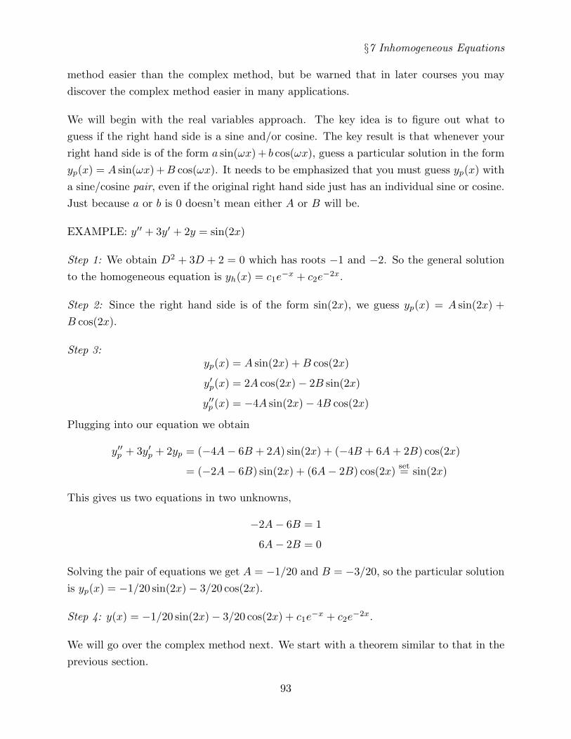
§7 Inhomogeneous Equations
method easier than the complex method, but be warned that in later courses you maydiscover the complex method easier in many applications.
We will begin with the real variables approach. The key idea is to figure out what toguess if the right hand side is a sine and/or cosine. The key result is that whenever yourright hand side is of the form a sin(ωx) + b cos(ωx), guess a particular solution in the formyp(x) = A sin(ωx) +B cos(ωx). It needs to be emphasized that you must guess yp(x) witha sine/cosine pair, even if the original right hand side just has an individual sine or cosine.Just because a or b is 0 doesn’t mean either A or B will be.
EXAMPLE: y′′ + 3y′ + 2y = sin(2x)
Step 1: We obtain D2 + 3D + 2 = 0 which has roots −1 and −2. So the general solutionto the homogeneous equation is yh(x) = c1e
−x + c2e−2x.
Step 2: Since the right hand side is of the form sin(2x), we guess yp(x) = A sin(2x) +B cos(2x).
Step 3:yp(x) = A sin(2x) +B cos(2x)
y′p(x) = 2A cos(2x)− 2B sin(2x)
y′′p (x) = −4A sin(2x)− 4B cos(2x)
Plugging into our equation we obtain
y′′p + 3y′p + 2yp = (−4A− 6B + 2A) sin(2x) + (−4B + 6A+ 2B) cos(2x)
= (−2A− 6B) sin(2x) + (6A− 2B) cos(2x) set= sin(2x)
This gives us two equations in two unknowns,
−2A− 6B = 1
6A− 2B = 0
Solving the pair of equations we get A = −1/20 and B = −3/20, so the particular solutionis yp(x) = −1/20 sin(2x)− 3/20 cos(2x).
Step 4: y(x) = −1/20 sin(2x)− 3/20 cos(2x) + c1e−x + c2e
−2x.
We will go over the complex method next. We start with a theorem similar to that in theprevious section.
93

Chapter 2: Linear Constant Coefficient Higher Order Equations
Theorem. If a, b and c are real and ay′′+by′+cy = f , then a(<[y])′′+b(<[y])′+c(<[y]) =<[f ] and a(=[y])′′ + b(=[y])′ + c(=[y]) = =[f ].
Proof: Take the real and imaginary parts of each side of the given equation ay′′ + by′ +cy = f .
This gives us a strategy to use with sines and cosines. We write them as the real part of acomplex exponential and then find a particular solution for the complex equation. Finallywe take the real part of the complex particular solution to find the particular solution tothe original real equation. This differs enough from the first paradigm that I will write itdown as a new paradigm.
Paradigm: y′′ + y′ − 2y = − cos(2x).
STEP 1: Find the general solution of the homogeneous equation.
The roots of D2 + D − 2 = 0 are −2 and 1 so the general solution of the homogeneousequation is yh(x) = c1e
−2x + c2ex.
STEP 2: Write the right hand side of the equation as the real part of a complex exponential.
− cos(2x) = <[−ei2x].
STEP 3: Find a particular solution to the corresponding complex equation.
Let yp denote a particular solution to y′′p + 2y′p − yp = −ei2x. Then we use the techniquesdeveloped earlier in this section to find yp(x).
SubStep 1: Guess the form of yp
yp = Ae2ix.
SubStep 2: Plug into the equation and solve for the undetermined coefficients.
yp = Ae2ix
y′p = 2iAe2ix
y′′p = −4Ae2ix
94

§7 Inhomogeneous Equations
Plugging into the equation we obtain
y′′p + y′p − 2yp = (−4Ae2ix) + (2iAe2ix)− 2(Ae2ix)
= (−4A+ 2iA− 2A)e2ix
= (−6 + 2i)Ae2ix set= −e2ix
Solving the last equation we find A = −1/(−6 + 2i) = 3/20 + 1/20i. So yp(x) = (3/20 +1/20i)e2ix.
STEP 4: Take the real part of the complex particular solution to find the real particularsolution.
yp(x) = <[yp(x)] = 3/20 cos(2x)− 1/20 sin(2x).
STEP 5: The general solution is y(x) = yp(x) + yh(x).
y(x) = 3/20 cos(2x)− 1/20 sin(2x) + c1e−2x + c2e
x.
We illustrate a few more possible difficulties in the final two examples.
EXAMPLE: y′′ + 3y′ + 2y = 3e−2x sin(x).
Step 1: The roots of D2 + 3D + 2 = 0 are −1 and −2 so the homogeneous solution isyh(x) = c1e
−x + c2e−2x.
Step 2: 3e−2x sin(x) = <[−3ie(−2+i)x]. (Note that we have to put the −3i to get a 3 aftermultiplying by i sin(x) in the identity for complex exponentials. It would also be possibleto write the real function as the imaginary part of a complex exponential rather than thereal part. In that case, we would have to take the imaginary part of the complex particularsolution in step 4.)
Step 3:
SubStep 1: yp(x) = Ae(−2+i)x
SubStep 2:yp(x) = Ae(−2+i)x
y′p(x) = (−2 + i)Ae(−2+i)x
y′′p (x) = (3− 4i)Ae(−2+i)x
95
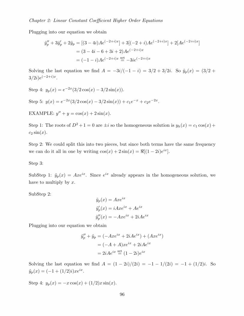
Chapter 2: Linear Constant Coefficient Higher Order Equations
Plugging into our equation we obtain
y′′p + 3y′p + 2yp = [(3− 4i)Ae(−2+i)x] + 3[(−2 + i)Ae(−2+i)x] + 2[Ae(−2+i)x]
= (3− 4i− 6 + 3i+ 2)Ae(−2+i)x
= (−1− i)Ae(−2+i)x set= −3ie(−2+i)x
Solving the last equation we find A = −3i/(−1 − i) = 3/2 + 3/2i. So yp(x) = (3/2 +3/2i)e(−2+i)x.
Step 4: yp(x) = e−2x(3/2 cos(x)− 3/2 sin(x)).
Step 5: y(x) = e−2x(3/2 cos(x)− 3/2 sin(x)) + c1e−x + c2e
−2x.
EXAMPLE: y′′ + y = cos(x) + 2 sin(x).
Step 1: The roots of D2 +1 = 0 are ±i so the homogeneous solution is yh(x) = c1 cos(x)+c2 sin(x).
Step 2: We could split this into two pieces, but since both terms have the same frequencywe can do it all in one by writing cos(x) + 2 sin(x) = <[(1− 2i)eix].
Step 3:
SubStep 1: yp(x) = Axeix. Since eix already appears in the homogeneous solution, wehave to multiply by x.
SubStep 2:yp(x) = Axeix
y′p(x) = iAxeix +Aeix
y′′p (x) = −Axeix + 2iAeix
Plugging into our equation we obtain
y′′p + yp = (−Axeix + 2iAeix) + (Axeix)
= (−A+A)xeix + 2iAeix
= 2iAeix set= (1− 2i)eix
Solving the last equation we find A = (1 − 2i)/(2i) = −1 − 1/(2i) = −1 + (1/2)i. Soyp(x) = (−1 + (1/2)i)xeix.
Step 4: yp(x) = −x cos(x) + (1/2)x sin(x).
96

§7 Inhomogeneous Equations
Step 5: y(x) = −x cos(x) + 1/2x sin(x) + c1 cos(x) + c2 sin(x).
After all these examples, the reader may have discovered the following general rules.
• If the right-hand side is of the form erx and erx is not already in the homogeneoussolution, then the guess should be Aerx.• If the right-hand side is of the form (anx
n + · · · a1x+ a0)erx with an 6= 0 and erx is notalready in the homogeneous solution, then the guess should be (Anx
n + · · ·A1x+A0)erx.
Note that while an 6= 0, the other aj terms may or may not be 0 in this case.• If the right-hand side is of the form (anx
n + · · · a1x+ a0)erx with an 6= 0 and xmerx isin the homogeneous solution, then the guess should be xm+1(Anx
n + · · ·A1x+A0)erx.
• If the right-hand side is of the form a sin(ωx) + b cos(ωx), guess A sin(ωx) + B cos(ωx).Note that you have to include both A and B even if a or b is 0.• You can also replace sines and cosines with complex exponentials to apply the aboverules to them.
Of course, if you misapply these rules all that will happen is that you will get stuck as wedid in the examples above where a wrong initial guess was made. In that case you justreconsider and guess again.
Exercises:
(1) y′′ + 3y′ + 2y = ex
(3) y′′ − 4y′ + 3y = e2x − e−2x
(5) y′′ + 2y′ − 3y = e−3x
(7) y′′ + 4y′ + 3y = cos(2x)
(9) y′′ − 2y′ − 15y = sin(x)− cos(x)
(2) y′′ − 5y′ + 6y = −e4x
(4) y′′ + y′ − 12y = xex
(6) y′′ + 2y′ + y = xe−x − 2e3x
(8) y′′ + 7y′ + 12y = ex cos(3x)
(10) y′′ + y = cos(x)
97
Chapter 2: Linear Constant Coefficient Higher Order Equations
(11) y′′ + 5y′ + 4y = e−x, y(0) = 0, y′(0) = 0
(12) y′′ − 3y′ − 4y = 3e−2x, y(0) = 1, y′(0) = 0
(13) y′′ + 4y′ + 4y = e−x + 2e2x, y(0) = 0, y′(0) = 1
(14) y′′ − y = sin(x), y(0) = 0, y′(0) = 0
(15) y′′ + 2y′ + 2y = ex(1 + cos(x)), y(0) = 3, y′(0) = 0
(16) y′′ + 3y′ + 2y = e3x, y(0) = 0, y′(0) = 0
(17) y′′ + y = cos(x), y(0) = 1, y′(0) = 1
(18) y′′ + 2y′ + 2y = ex, y(0) = 1, y′(0) = 0
(19) y′′ + 2y′ + y = e−x, y(0) = 0, y′(0) = 0
(20) y′′′ − y′ = e2x, y(0) = 1, y′(0) = 0, y′′(0) = 0
For problems 21 through 25, guess the form of the particular solution, but don’t solve theequations.
(21) y′′ + y′ + y = ex sin(2x)− x2
(22) y′′ − y′ + 3y = e2x − xex + cos(x)
(23) y′′ + y = ex sin(2x)− ex cos(3x− π/7)
(24) y′′ − y = x3ex + x2 cos(x)
(25) y′′ + 4y′ + y = x2e−3x cos(2x) + xe−3x sin(2x)
§8 Variation of Parameters
Discussion: The method of undetermined coefficients is the most efficient way to solvean inhomogeneous equation if we can guess the proper form for the particular solution.Unfortunately we can’t always guess the proper form. If we can find the general solutionto the homogeneous equation, the method of variation of parameters will always work.Because the method is complicated, we will only cover the second order case. Considerthe following example
y′′ + y = tan(x)
We first find two linearly independent solutions to the homogeneous equation y′′ + y = 0.In this case two linearly independent solutions are cos(x) and sin(x). We now guess thatthe solution to the inhomogeneous equation will take the form
y(x) = u(x) cos(x) + v(x) sin(x)
98

§8 Variation of Parameters
Differentiating this yields
y′(x) = −u(x) sin(x) + v(x) cos(x) + u′(x) cos(x) + v′(x) sin(x)
We should now differentiate this again to compute y′′ but this is getting ugly. y′′ will have 6terms. At this point I observe I have 2 degrees of freedom in my guess for the solution (i.e.2 unknown functions) and I only need to satisfy one equation. With 2 unknown functionsI should be able to satisfy 2 equations and I will now tack on the additional condition thatbesides solving the original problem, y′′ + y = tan(x), I will choose u and v so that
u′(x) cos(x) + v′(x) sin(x) = 0.
Using this I can then get
y′(x) = −u(x) sin(x) + v(x) cos(x)
and I then differentiate again to get
y′′(x) = −u(x) cos(x)− v(x) sin(x)− u′(x) sin(x) + v′(x) cos(x)
So plugging into y′′ + y = tan(x) we get
y′′ + y =− u(x) cos(x)− v(x) sin(x)− u′(x) sin(x) + v′(x) cos(x)
+ u(x) cos(x) + v(x) sin(x)set= tan(x)
From which we get the equation
−u′(x) sin(x) + v′(x) cos(x) = tan(x)
We now have two equations for u′(x) and v′(x).
(1)u′(x) cos(x) + v′(x) sin(x) = 0
−u′(x) sin(x) + v′(x) cos(x) = tan(x)
Multiplying the first equation by sin(x) and the second equation by cos(x) and adding weobtain
v′(x)(sin2(x) + cos2(x)) = sin(x)
v′(x) = sin(x)
v(x) = − cos(x) + C1
99

Chapter 2: Linear Constant Coefficient Higher Order Equations
Multiplying the first equation in (1) by cos(x) and the second equation in (1) by − sin(x)and adding we obtain
u′(x)(cos2(x) + sin2(x)) = − sin2(x)/ cos(x)
u′(x) = − sin2(x)/ cos(x)
u(x) = sin(x)− log(
sin(x) + 1cos(x)
)+ C2
Finally we get
y(x) = sin(x) cos(x)− log(
sin(x) + 1cos(x)
)cos(x) + C2 cos(x)− cos(x) sin(x) + C1 sin(x)
= − log(
sin(x) + 1cos(x)
)cos(x) + C2 cos(x) + C1 sin(x)
In this one case, I do not advise you to learn the procedure for solving inhomogeneousequations using variation of parameters. The manipulations given above are complicatedand most students have lots of trouble with them. Using them, I can derive the followingformula and I advise you to just copy down the formula on your crib sheet and use itwhenever necessary.
Theorem. If y1(x) and y2(x) are two linearly independent solutions to the second order
linear homogeneous equation y′′(x) + b(x)y′(x) + c(x)y(x) = 0 then
y(x) = −y1(x)∫ x
x0
y2(s)g(s)W (y1, y2)(s)
ds+ y2(x)∫ x
x0
y1(s)g(s)W (y1, y2)(s)
ds+ C1y1(x) + C2y2(x)
is the general solution to the inhomogeneous equation y′′(x) + b(x)y′(x) + c(x)y(x) = g(x)where x0, C1 and C2 are arbitrary constants and W (y1, y2)(s) is the Wronskian.
This looks at first glance to have three arbitrary constants but in fact it only has two. Anygiven solution can be obtained with every choice of x0 by making the right choice of C1
and C2. The advantage of this form is that while we often won’t be able to evaluate theintegrals, we will always be able to evaluate any definite integral from x0 to x0. So if wehave an initial value problem with the values given at x0, we will be able to work out thevalues of C1 and C2 even if we can’t compute the integrals directly.
Paradigm: Solve x2y′′ + xy′ − 4y = x given that two linearly independent solutions ofthe corresponding homogeneous equation are y1(x) = x2 and y2(x) = x−2.
100

§8 Variation of Parameters
STEP 1: Find two linearly independent solutions of the corresponding homogeneous prob-lem.
Here we are given that two solutions are y1(x) = x2 and y2(x) = x−2.
STEP 2: Evaluate the solution of the inhomogeneous problem using the formula.
W (y1, y2)(s) = s2 ×−2s−3 − 2s× s−2 = −4s−1
Pick x0 = 0 for convenience∫ x
0
s−2s
−4s−1ds =
∫ x
0
−14ds = −x/4∫ x
0
s2s
−4s−1ds =
∫ x
0
−s4
4ds = −x5/20
So we get
y(x) = −x2 ×−x/4 + x−2 ×−x5/20 + C1x2 + C2x
−2
= x3/5 + C1x2 + C2x
−2
EXAMPLE: Solve the initial value problem
y′′ + 6y′ + 5y =√x, y(1) = 0, y′(1) = 0
FIRST: Find the general solution
Step 1: The homogeneous equation is y′′ + 6y′ + 5y = 0
SubStep 1: (D2 + 6D + 5)y = (D + 5)(D + 1)y = 0
SubStep 2: roots are −5 and −1
SubStep 3: The general solution is C1e−5x + C2e
−x and e−5x and e−x are two linearlyindependent solutions of the homogeneous equation.
Step 2:
W (e−5x, e−x) = e−5x ×−e−x − (−5e−5x × e−x) = 4e−6x
101
Chapter 2: Linear Constant Coefficient Higher Order Equations
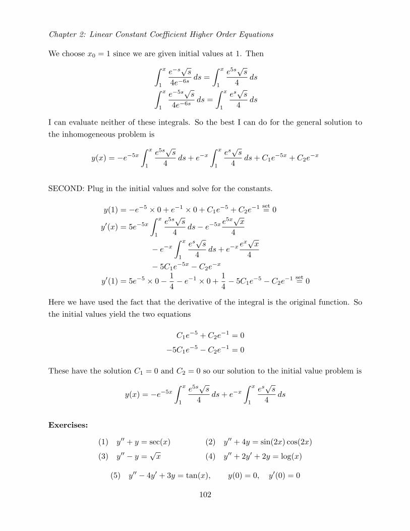
We choose x0 = 1 since we are given initial values at 1. Then∫ x
1
e−s√s
4e−6sds =
∫ x
1
e5s√s
4ds∫ x
1
e−5s√s
4e−6sds =
∫ x
1
es√s
4ds
I can evaluate neither of these integrals. So the best I can do for the general solution tothe inhomogeneous problem is
y(x) = −e−5x
∫ x
1
e5s√s
4ds+ e−x
∫ x
1
es√s
4ds+ C1e
−5x + C2e−x
SECOND: Plug in the initial values and solve for the constants.
y(1) = −e−5 × 0 + e−1 × 0 + C1e−5 + C2e
−1 set= 0
y′(x) = 5e−5x
∫ x
1
e5s√s
4ds− e−5x e
5x√x
4
− e−x
∫ x
1
es√s
4ds+ e−x e
x√x
4− 5C1e
−5x − C2e−x
y′(1) = 5e−5 × 0− 14− e−1 × 0 +
14− 5C1e
−5 − C2e−1 set= 0
Here we have used the fact that the derivative of the integral is the original function. Sothe initial values yield the two equations
C1e−5 + C2e
−1 = 0
−5C1e−5 − C2e
−1 = 0
These have the solution C1 = 0 and C2 = 0 so our solution to the initial value problem is
y(x) = −e−5x
∫ x
1
e5s√s
4ds+ e−x
∫ x
1
es√s
4ds
Exercises:
(1) y′′ + y = sec(x)
(3) y′′ − y =√x
(2) y′′ + 4y = sin(2x) cos(2x)
(4) y′′ + 2y′ + 2y = log(x)
(5) y′′ − 4y′ + 3y = tan(x), y(0) = 0, y′(0) = 0
102

§9 Boundary Value Problems
§9 Boundary Value Problems
A second order equation will have two arbitrary constants in its general solution, so if youwant to specify a particular solution you should expect to require two additional conditions.So far, the conditions we have considered have always been initial values, where you aregiven the value of the function and its derivative at a point. Physically, this correspondsto knowing the position and velocity at a given time. But it is quite possible to be givenother types of conditions. Another common example is boundary conditions, where youare told the value of the function at two different points. Physically, this corresponds toknowing the position at two different times. At first glance, there appears to be littledifferent about such problems. You just find the general solution, then plug in the twoconditions and solve to find the values of the constants. This is indeed how you go aboutsolving the problem. But there turn out to be various interesting difficulties that arise inboundary value problems that don’t arise in initial value problems.
EXAMPLE: Solve the boundary value problem y′′ + y = 0, y(0) = 1, y(1) = 2.
FIRST: Find the general solution. This is a homogeneous equation so it is easy to findthat the general solution is y(x) = c1 sin(x) + c2 cos(x).
SECOND: Plug in the boundary values and solve for the constants.
y(0) = c1 sin(0) + c2 cos(0) = c2set= 1
y(1) = c1 sin(1) + c2 cos(1) set= 2
Solving the equations we get
c1 =2− cos(1)
sin(1)c2 = 1
so the solution is y(x) = 2−cos(1)sin(1) sin(x) + cos(x).
That didn’t seem very exciting. But consider the next example.
EXAMPLE: y′′ + y = 0, y(0) = 1, y(π) = 2.
FIRST: As before, we find the general solution is y(x) = c1 sin(x) + c2 cos(x).
103
Chapter 2: Linear Constant Coefficient Higher Order Equations
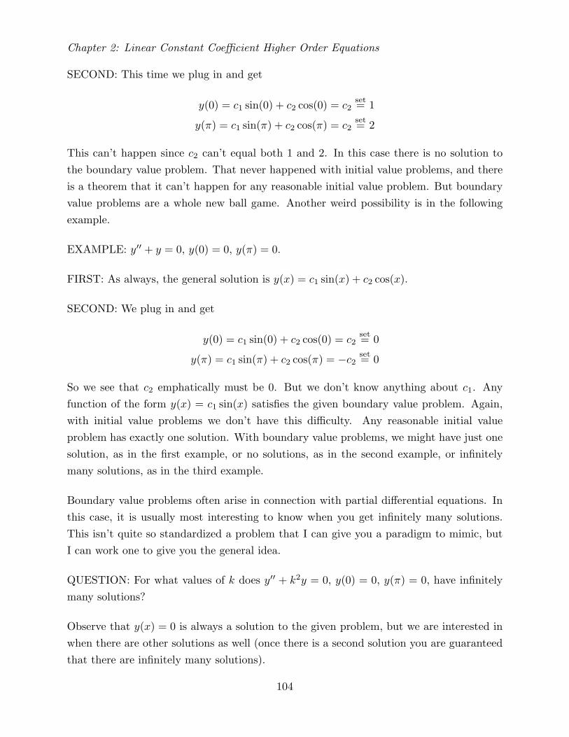
SECOND: This time we plug in and get
y(0) = c1 sin(0) + c2 cos(0) = c2set= 1
y(π) = c1 sin(π) + c2 cos(π) = c2set= 2
This can’t happen since c2 can’t equal both 1 and 2. In this case there is no solution tothe boundary value problem. That never happened with initial value problems, and thereis a theorem that it can’t happen for any reasonable initial value problem. But boundaryvalue problems are a whole new ball game. Another weird possibility is in the followingexample.
EXAMPLE: y′′ + y = 0, y(0) = 0, y(π) = 0.
FIRST: As always, the general solution is y(x) = c1 sin(x) + c2 cos(x).
SECOND: We plug in and get
y(0) = c1 sin(0) + c2 cos(0) = c2set= 0
y(π) = c1 sin(π) + c2 cos(π) = −c2set= 0
So we see that c2 emphatically must be 0. But we don’t know anything about c1. Anyfunction of the form y(x) = c1 sin(x) satisfies the given boundary value problem. Again,with initial value problems we don’t have this difficulty. Any reasonable initial valueproblem has exactly one solution. With boundary value problems, we might have just onesolution, as in the first example, or no solutions, as in the second example, or infinitelymany solutions, as in the third example.
Boundary value problems often arise in connection with partial differential equations. Inthis case, it is usually most interesting to know when you get infinitely many solutions.This isn’t quite so standardized a problem that I can give you a paradigm to mimic, butI can work one to give you the general idea.
QUESTION: For what values of k does y′′ + k2y = 0, y(0) = 0, y(π) = 0, have infinitelymany solutions?
Observe that y(x) = 0 is always a solution to the given problem, but we are interested inwhen there are other solutions as well (once there is a second solution you are guaranteedthat there are infinitely many solutions).
104

§10 Partial Differential Equations
The way to begin such a problem is to write out the general solution and plug in theboundary values. The general solution to y′′ + k2y = 0 is y(x) = c1 sin(kx) + c2 cos(kx).We plug in the boundary values to get
y(0) = c1 sin(0) + c2 cos(0) = c2set= 0
y(π) = c1 sin(kπ) + c2 cos(kπ) set= 0
From the first equation we know c2 must be 0. Plugging this into the second equation weget c1 sin(kπ) = 0, so either c1 = 0 or sin(kπ) = 0. If c1 = 0, we just get the solutiony(x) = 0, so if we want infinitely many solutions we need sin(kπ) = 0. This happensexactly when k is an integer.
Exercises:
Solve the following boundary value problems if possible. (1) y′′ + 3y′ + 2y = 0, y(0) = 0,y(1) = 1.
(2) y′′ + 2y′ + 10y = 0, y(0) = 1, y(1) = 0.
(3) y′′ + 10y′ + 21y = 0, y(0) = 4, y(1) = −1.
(4) y′′ + 9y′ + 10y = 0, y(0) = 0, y(π) = 5.
(5) y′′ + y = 0, y(0) = 0, y(π/2) = 0.
(6) y′′ + 4y = 0, y(0) = 0, y(π/2) = 0.
(7) y′′ + 9y = 0, y(0) = 0, y(π/2) = 0.
(8) y′′ + 16y = 0, y(0) = 0, y(π/2) = 0.
(9) y′′ − y = 0, y(0) = 0, y(π/2) = 0.
(10) y′′ = 0, y(0) = 0, y(π/2) = 0.
(11) For what values of k does y′′ + k2y = 0, y(0) = 0, y(π/2) = 0 have infinitely manysolutions?
(12) For what values of k does y′′ + k2y = 0, y(0) = 0, y(1) = 0 have infinitely manysolutions?
(13) For what values of ` does y′′+y = 0, y(0) = 0, y(`) = 0 have infinitely many solutions?
(14) For what values of k does y′′ + k2y = 0, y(0) = 0, y(π) = 1 have no solutions?
(15) For what values of ` does y′′ + y = 0, y(0) = 0, y(`) = 0 have no solutions?
§10 Partial Differential Equations
105
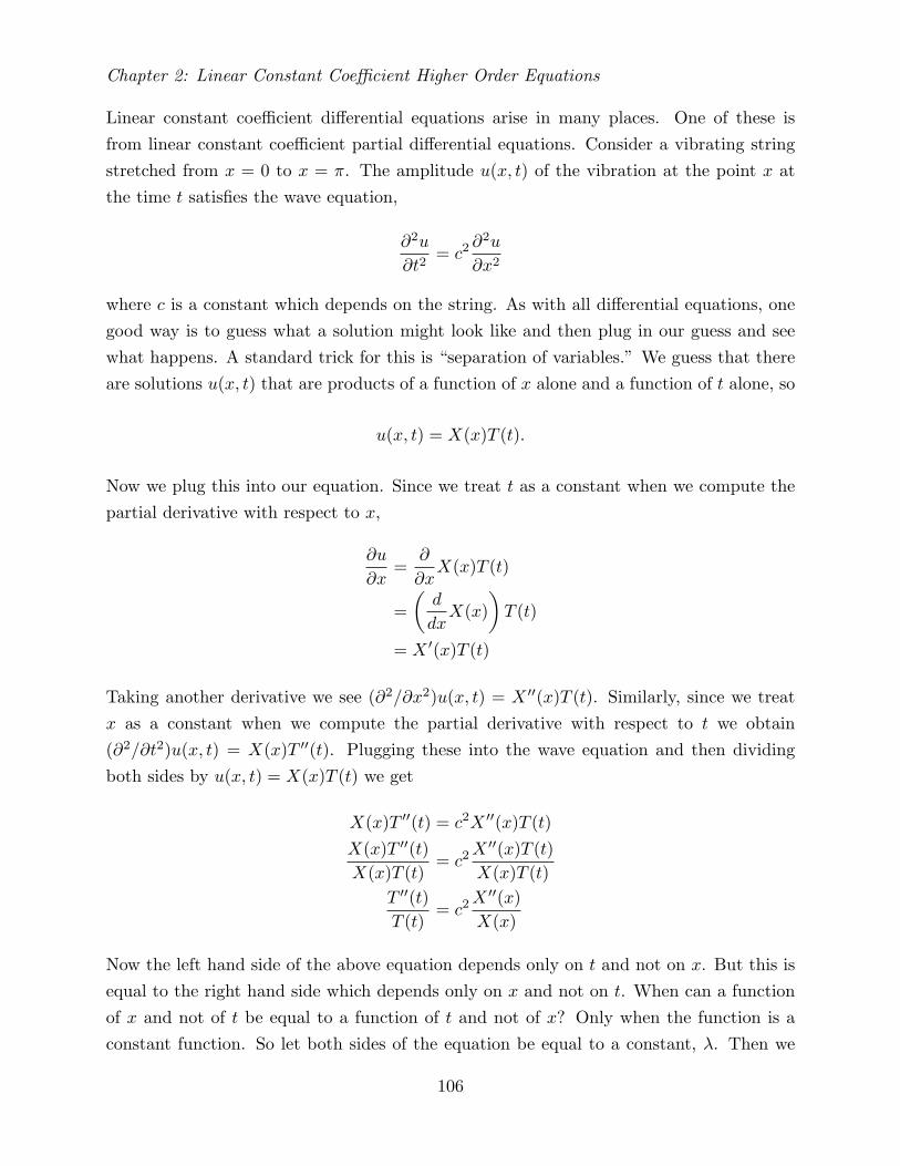
Chapter 2: Linear Constant Coefficient Higher Order Equations
Linear constant coefficient differential equations arise in many places. One of these isfrom linear constant coefficient partial differential equations. Consider a vibrating stringstretched from x = 0 to x = π. The amplitude u(x, t) of the vibration at the point x atthe time t satisfies the wave equation,
∂2u
∂t2= c2
∂2u
∂x2
where c is a constant which depends on the string. As with all differential equations, onegood way is to guess what a solution might look like and then plug in our guess and seewhat happens. A standard trick for this is “separation of variables.” We guess that thereare solutions u(x, t) that are products of a function of x alone and a function of t alone, so
u(x, t) = X(x)T (t).
Now we plug this into our equation. Since we treat t as a constant when we compute thepartial derivative with respect to x,
∂u
∂x=
∂
∂xX(x)T (t)
=(d
dxX(x)
)T (t)
= X ′(x)T (t)
Taking another derivative we see (∂2/∂x2)u(x, t) = X ′′(x)T (t). Similarly, since we treatx as a constant when we compute the partial derivative with respect to t we obtain(∂2/∂t2)u(x, t) = X(x)T ′′(t). Plugging these into the wave equation and then dividingboth sides by u(x, t) = X(x)T (t) we get
X(x)T ′′(t) = c2X ′′(x)T (t)X(x)T ′′(t)X(x)T (t)
= c2X ′′(x)T (t)X(x)T (t)
T ′′(t)T (t)
= c2X ′′(x)X(x)
Now the left hand side of the above equation depends only on t and not on x. But this isequal to the right hand side which depends only on x and not on t. When can a functionof x and not of t be equal to a function of t and not of x? Only when the function is aconstant function. So let both sides of the equation be equal to a constant, λ. Then we
106

§10 Partial Differential Equations
have reduced the second order partial differential equation to two second order ordinarydifferential equations:
T ′′(t)T (t)
= λ
c2X ′′(x)X(x)
= λ
We can now solve these equations simultaneously. If λ > 0, then it has a square root say√λ = µ so λ = µ2 and the solutions of the ordinary differential equations are
T ′′(t) = µ2T (t)
T ′′(t)− µ2T (t) = 0
(D2 − µ2)T (t) = 0
T (t) = C1eµt + C2e
−µt
c2X ′′(x) = µ2X(x)
c2X ′′(x)− µ2X(x) = 0
(c2D2 − µ2)X(x) = 0
X(x) = C3eµx/c + C4e
−µx/c
and so we have a collection of solutions of the partial differential equation of the form
u(x, t) = (C3eµx/c + C4e
−µx/c)(C1eµt + C2e
−µt)
Of course, it is also possible that λ is negative, in which case we let√−λ = ν so λ = −ν2
and the solutions of the ordinary differential equations are
T ′′(t) = −ν2T (t)
T ′′(t) + ν2T (t) = 0
(D2 + ν2)T (t) = 0
T (t) = C1 cos(νt) + C2 sin(νt)
c2X ′′(x) = −ν2X(x)
c2X ′′(x) + ν2X(x) = 0
(c2D2 + ν2)X(x) = 0
X(x) = C3 cos(νx/c) + C4 sin(νx/c)
and so we have another collection of solutions of the partial differential equations of theform
u(x, t) = (C1 cos(νt) + C2 sin(νt))(C3 cos(νx/c) + C4 sin(νx/c))
Finally, if λ = 0 then the solutions of the ordinary differential equation are
T ′′(t) = 0
T (t) = C1 + C2t
c2X ′′(x) = 0
X(x) = C3 + C4x
and so we have one last collection of solutions of the partial differential equation of theform
u(x, t) = (C1 + C2t)(C3 + C4x)
107

Chapter 2: Linear Constant Coefficient Higher Order Equations
The wave equation is a linear partial differential equation, which means that sums ofsolutions are still solutions, just as for linear ordinary differential equations. So now wecan form lots of different solutions out of our various collections of solutions. Usually wewill want to find solutions that have particular properties. For example, if our string istacked down at x = 0 and x = π so that the amplitude of vibration is always 0 at thosepoints, then we want u(0, t) = u(π, t) = 0 for all t. This condition will eliminate many ofthe different solutions given above (see problem 5). It turns out that all solutions of thewave equation satisfying the condition that the endpoints are tacked down can be writtenas linear combinations of the solutions we have found, so we will have the general solutionto the wave equation subject to this condition. But the situation is more complicated thanfor ordinary differential equations, because while we have eliminated many of the differentsolutions with our tacking down condition, we still have infinitely many solutions left soour general solution has infinitely many arbitrary constants. But that is a problem bestleft to a later course in Fourier series, or better yet partial differential equations. For now,we will settle for noting that the linear constant coefficient ordinary differential equationswe have been considering in this chapter often come up in solving linear constant coefficientpartial differential equations.
Exercises:(1) Find solutions in the form u(x, t) = X(x)T (t) for the heat equation ∂u/∂t = κ2∂2u/∂x2.(2) Find solutions in the form u(x, y) = X(x)Y (y) for Laplace’s equation ∂2u/∂x2 +∂2u/∂y2 = 0.(3) Find solutions in the form u(x, t) = X(x)T (t) for the equation ∂u/∂t = ∂2u/∂x2 − u
(heat equation with cooling).(4) Find solutions in the form u(x, y) = X(x)Y (y) for Poisson’s equation ∂2u/∂x2 +∂2u/∂y2 = u.(5) Show that the only solutions of the form u(x, t) = X(x)T (t) to the wave equation thatsatisfy u(0, t) = u(π, t) = 0 for all t are u(x, t) = (C1 cos(cnt) +C2 sin(cnt)) sin(nx) wheren is a positive integer.
§11 Free Motion
Consider a mass on a spring. The forces acting on the mass are gravity with a force mg,where m is the mass and g is the acceleration of gravity (9.8m/sec2), the restoring forceof the spring with a force −kl, where k is the spring constant, l is how much the spring is
108
Related Documents