Using FDTD for Other Types of Simulation In this chapter, we will discuss the use of the FDTD method for applications other than electro ma gnetics . The firstappl ic at ion is an acousti csimula ti on problem. The math emat ic s of ac ou st ic s is similarto el ec tromag ne tics [1] ,soit is nat uralthat the develo pm en ts of FDTD are used in aco usticsimulati on[2, 3]. The secondexampleis the si mulation of the Sc hr oedinger equation ,whichis at the heartofquantum me ch anic s. Quantum me chan ic s is radica llydi ff er en t from both aco ust ics and ele ctr oma gne tic s. However, the Schroedi ng er equatio nis still a wave equ at ionandit lends its elf to si mulation withFDTD.In both cases,onl y si mpleexamplesof one- dimens iona l simula tio ns are pre sen ted . 6.1 THE ACOUSTIC FDTD FORMULATION In the fo ll owin g de velopment, we willdeal only with press urewavesand ignoreelastic waves. We start with the fi rs t- order acou st ic eq ua ti on s, a " 8 t P (x , t) = V · u (6.1a) d PoP, dtu(x,t) = Vp(x,t), (6.1b) where pix, t) is the pressurefield [F 1m2] = [kgl(m - sec 2 ) ] , u(x, t ) is the vect orvelocityfield [mlsec] , Po is the ma ss densityof water [kg/m 3 ] , P, is the relative (t o water )massdensit y of the medi um, " isthe compressibilit y of the medium [(m - sec 2 ) / kg] . (Table 6.1) Not ice that waterhas been chosenas thebackgroundmedi uminst ead of air. The compress ibilityis 1 I K=--= , P · c 2 Po · Pr . c 2 wher e c is the velocityof sound. (6.2) 133

Welcome message from author
This document is posted to help you gain knowledge. Please leave a comment to let me know what you think about it! Share it to your friends and learn new things together.
Transcript
8/7/2019 6_Using FDTD for Other Types of Simulation
http://slidepdf.com/reader/full/6using-fdtd-for-other-types-of-simulation 1/14
Using FDTD for Other Types
of Simulation
In this chapter, we will discuss the use of the FDTD method for applications other than
electromagnetics. The firstapplication is anacousticsimulationproblem.Themathematics of
acoustics is similarto electromagnetics [1], so it is naturalthat thedevelopments ofFDTDare
used in acousticsimulation[2, 3]. The secondexampleis the simulation of the Schroedinger
equation,whichisattheheartofquantummechanics. Quantummechanics isradicallydifferent
fromboth acoustics and electromagnetics. However, theSchroedingerequationis still a wave
equationand it lendsitself to simulation withFDTD.In both cases,only simpleexamplesofone-dimensional simulations are presented.
6.1 THEACOUSTIC FDTDFORMULATION
In thefollowing development, wewilldealonlywithpressurewavesandignoreelasticwaves.Westartwith the first-order acoustic equations,
a" 8t P (x , t) = V· u (6.1a)
d
PoP, dtu(x,t) =Vp(x,t), (6.1b)
where pix, t) is the pressurefield [F1m2]= [kgl(m - sec2) ] ,
u(x, t) is the vectorvelocityfield [mlsec] ,
Po is the massdensityof water [kg/m3] ,
P, is the relative(to water)massdensityof themedium,
" is the compressibility of the medium [(m - sec2) / kg] . (Table 6.1)
Notice that waterhas been chosen as thebackgroundmediuminsteadof air. The compress
ibilityis
1 IK=--= ,P · c2 Po · Pr . c2
wherec is the velocityof sound.
(6.2)
133
8/7/2019 6_Using FDTD for Other Types of Simulation
http://slidepdf.com/reader/full/6using-fdtd-for-other-types-of-simulation 2/14
134 Chapter 6 • Using FDTD for OtherTypes of Simulation
TABLE6.1 Acoustic Properties of a Few Materials
Material
1. Water
2. Air
3. Metal
Speed ofSound (m/sec)
1500
343
5900
1000
1.21
7800
Compressibility (m • s2/kg)
4.4 X 10⁻⁸
7.02 X 10⁻⁶
Eq. (6.1a) can be written
dp(x, y, z. t) 1 [dUx(X, y, z, t) duy(x, y, z, t) duz(x, y, Z, t ) ]- - - -= + + .
dt K(X,y,Z) dx dy dz
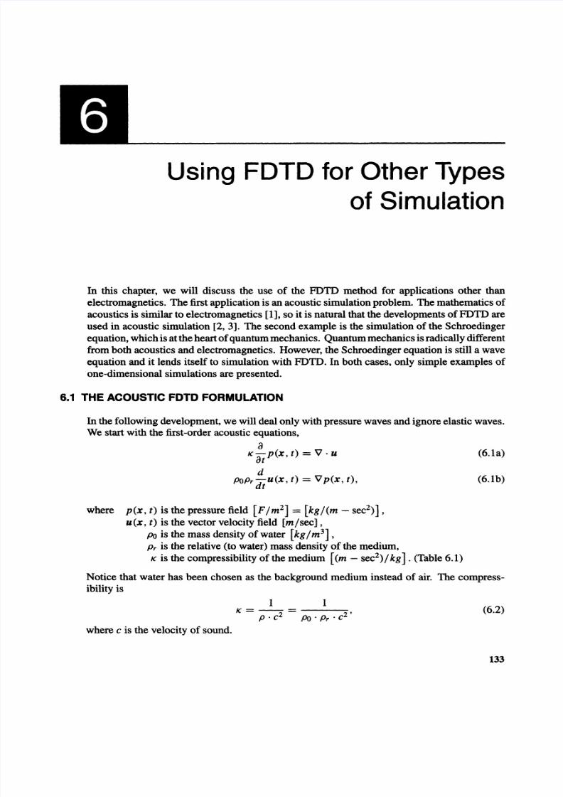
We will use a differencing scheme similar to Yee's FDTD for electromagnetics [4]; however,
we will assume that the pressure locations are at nodes in a three-dimensional lattice, and that
the velocities are located between the nodes, as shown in Fig. 6.1.
z
/'
//
/'
/
III
III
(i.j.k + 1).... _----- ....
uz(i,j,k + 1/2)
uy(i,j + 1/2,k)
//'
//
/'
y
Figure 6.1 The acoustic Yeecell.
Using first-order differencing in time and space, Eq. (6.1.a) can be written
pn+I/2(i, i, k) - pn-I/2(i, i, k) = 1 [ U ~ ( i + 1/2, j , k) - u ~ ( i - 1/2, j , k)]6.t K(i, j , k) Sx
1 [U;(i, j, k + 1/2) - u;(i, j, k - 1/2)]+ «(i, j, k) !!.y
1 [ U ~ ( i , i, k + 1/2) - u ~ ( i , j, k - 1/2)] .
+ «(i, j, k) !!.Z
First, the compressibility will be replaced by Eq. (6.2). Then L).t will be moved to the right
side, giving a difference equation suitable to the FDTD formulation:
n+l/2(. . k) - n-l/2(. . k) + 6.t· POPrc2
• [ n(. + 1/2 . k) _ n(" - 1/2 "k)]p I,J, -p I ,J, 6.x Ux I .r. ux ' ,J ,
~ · POPrc2
[ n ( " . 1/2 k) n(" . 1/2 k)]+ " u y I, I + , - uy I, l - ,dy
d t . POPrc2
[n( . i. k 1/2) n ( . . k 1/2)]+ · Uz I, j , + - Uz I, j , - ·dz
(6.3)
8/7/2019 6_Using FDTD for Other Types of Simulation
http://slidepdf.com/reader/full/6using-fdtd-for-other-types-of-simulation 3/14
Section 6.1 • The Acoustic FDTD Formulation 135
A similar procedure in Eq. (6.lb) yields three equations of the type
un+1/2(i j. k + 1/2) = un- 1/2(i j. k + 1/2)
z " z" Ilt (6.4)
+ C ' k+1/2) .. Il· [pn(i , j ,k+1)-pn(i , j ,k)] .P, r, t , Po z
Obviously, equations in the X and Y direction would be similar. Wewill limit ourselvesto a simple one-dimensional problem in the Z direction and rewrite Eqs. (6.3) and (6.4) as
follows:
pn+l/2(k) = pn-l/2(k) + ga(k). [ u ~ ( k + 1/2,) - u ~ ( k - 1/2)] (6.5a)
u ~ + l ( k + 1/2) = u ~ ( k + 1/2) + gb(k + 1/2) . [pn+l/2(k + 1) - pn+l/2(k)] , (6.5b)
where we have the parameters
ga(k) = Il t · PoPr · c2
~ ~
gb(k + 1/2) = (k 1/2) ·P + ·Po· ~
(6.6a)
(6.6b)
Notice that we have chosen to write ga in terms of the speed of sound and the pressure
rather than the compressibility since these are the parameters that are most widely used.
As before, I:1t is chosen after ~ is chosen according to
~ ~ t < -- cmax '
where emu is the fastest velocity of sound that we encounter. We will suppose that this will
be metal, in which the velocity of sound is 5900 meters per second. Just to give ourselves a
margin, we will take
~ ~ t = - .1()4
Since Po = 1000 kg/m, Eqs. (6.6) become
ga(k) = 10-1 • p, (k) c2 (k)
10-7
gb(k + 1/2) = k /'p,( + 1 2)
(6.7a)
(6.7b)
For water, which we will use as our backgroundmedium, Eqs. (6.7a) and (6.Th) tum out to be
ga(k) = 10-1 . P, (k) c; (k) = 10-1. 1 . (1, 500)2 = 2.25 X 10⁵ (6.8a)
gb(k + 1/2) = 10-7. (6.8b)
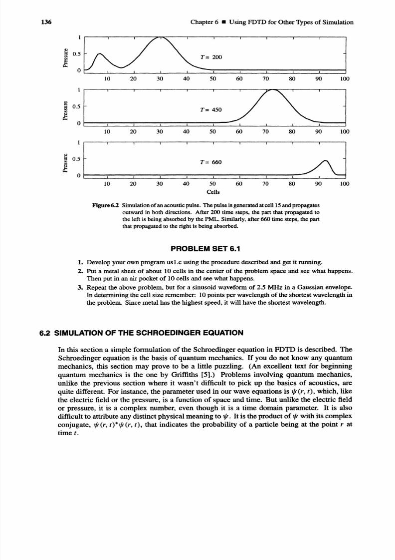
The program us l.c at the end of the chapter is a one-dimensional acoustic simulation
program. In its present form, it is only simulating water. Figure 6.2 shows the result. A pulse
is generated at one end and subtracted out at the other. So where did the PML come from?
Here is how this program was developed: I went back and made a copy of the program
fdld_l.l.c. Using the text editor, I replaced ex with p, and hy with u. Then I went to the
program we developed in Chapter 5 to simulate microstrip antennas, and I took the PML from
the lD incident buffer and copied it over. I added the parameters ga and gb, changed someconstants, and so forth, and there it was! The entire process took about 30 minutes. The point
is, an acoustic simulation program, complete with PML, was written by using the ideas we
had already developed for EM simulation.
8/7/2019 6_Using FDTD for Other Types of Simulation
http://slidepdf.com/reader/full/6using-fdtd-for-other-types-of-simulation 4/14
136 Chapter 6 • Using FDTD for Other Types of Simulation
OL--_--L__ __ ___J .__ ___J""___L...___ L____ .L _ .___ . .L._.__ ..L__ ___J
10 20 30 40 50 60 70 80 90 100
O t - - - ~ - - ~ - - ~ - - ~ - - ~ - - - -10 20 30 40 50 60 70 80 90 100
10000000
Cells
T= 660
40000
o . - . - ~ - - ~ - - ~ - - ~ - - ~ ~ - - ~ - - ~ - - . . . . . . - - " "
Figure6.2 Simulation ofan acoustic pulse. The pulse is generated atcell IS and propagates
outward in both directions. After 200 time steps, the part that propagated to
the left is being absorbed by the PML. Similarly, after 660 time steps, the part
that propagated to the right is being absorbed.
PROBLEM SET 6.1
1. Develop your own program usl. c using the procedure described and get it running.
2. Put a metal sheet of about 10 cells in the center of the problem space and see what happens.
Then put in an air pocket of 10 cells and see what happens.
3. Repeat the above problem, but for a sinusoid waveform of 2.5 MHz in a Gaussian envelope.
In determining the cell size remember: 10points per wavelength of the shortest wavelength in
the problem. Since metal has the highest speed, it will have the shortest wavelength.
6.2 SIMULATION OF THE SCHROEDINGER EQUATION
In this section a simple formulation of the Schroedinger equation in FDTD is described. The
Schroedinger equation is the basis of quantum mechanics. If you do not know any quantum
mechanics, this section may prove to be a little puzzling. (An excellent text for beginning
quantum mechanics is the one by Griffiths [5].) Problems involving quantum mechanics,
unlike the previous section where it wasn't difficult to pick up the basics of acoustics, are
quite different. For instance, the parameter used in our wave equations is 1/I(r, t) , which, like
the electric field or the pressure, is a function of space and time. But unlike the electric field
or pressure, it is a complex number, even though it is a time domain parameter. It is also
difficult to attribute any distinct physical meaning to 1/1. It is the product of 1/1 with its complex
conjugate, 1/J(r, t)*1/J(r, t), that indicates the probability of a particle being at the point r attime t.
8/7/2019 6_Using FDTD for Other Types of Simulation
http://slidepdf.com/reader/full/6using-fdtd-for-other-types-of-simulation 5/14
Section 6.2 • Simulation of the Schroedinger Equation
6.2.1 Formulating the Schroedinger Equation into FDTD
The time-dependent Schroedinger equation is given by [5-8]
01/l(r, t) n2in = --V 2
1/1 (r , t) + VCr, t) ·1/I(r, t)at 2m
ora1/l(r, t) n i
=i -\721/1(r, t) - t;"V (r, t) ·1/I(r, t) ,at 2m n
137
(6.9)
(6.10)
where m is the mass of the particle [kg],
Ii = 1.054 X 10⁻³⁴ [J - sec] is Plank's constant,
V is the potential [J]. (It will often bemore convenient to express
the potential in electron volts (eV), where 1 eV = 1.602 x 10⁻¹⁹J.)
Toavoid using complex numbers, we will split the variable 1/I(r, t) into its real and imaginary
components
1/1(r, t) = 1/1real(r, t) + i1/Iimag (r, t) . (6.11)
Inserting Eq. (6.11) into Eq. (6.10) and separating real and imaginary parts results in the
following coupled set of equations:
al/Jreal (r, t) n 2 1at = - 2m . V 1/Iimag(r, t) + hV 1frimag(r, t) (6.12a)
a1/limag(r, t) Ii 2 1at = 2m · V 1frreal(r, t) - hV 1/Ireal(r, t) . (6.12b)
We begin by assuming a one-dimensional space, arbitrarily taking the z direction. Starting
with Eq. (6.12a), the finite difference approximations in space and time result in
1/I:zeal (k) - 1 / I ~ ~ 1 (k)~ -a,,,n-I/2(k 1) 2-a,,,n-I/2(k) -a,,,n-l/2(k 1
Ii o/imag + - o/imag + o/imag -) 1 n-I/2= - 2m (.6.z)2 + h, V(k) '1/!imag (k),
from which we get
1/J:'eal (k) = 1 / J ~ - ; / (k)
_~
!!:-. [-a'I'!,-1/2(k+ 1) _ 2-a'I'.n-l/2(k) + -a'I'!,-1/2(k - 1)]~ Z 2m o/tmag o/tmag o/tmag (6.13)
~ n-I/2+r;V(k)·1/I imag (k).
We assume we are simulating an electron and therefore we will take m to be the mass of an
electron. Wewill take ~ to be one-tenth of an Angstrom, so
m = 9.1 x 10⁻³¹ [kg]
~ = 1 X 10-11 [m].
At this point, we don' t know what the time step, ~ t should be. Unfortunately, there is
no specific Courant condition to guide us, as was the case in EM simulation. We will startby assigning what seems to be a "reasonable" number, i.e., something that will likely keep
8/7/2019 6_Using FDTD for Other Types of Simulation
http://slidepdf.com/reader/full/6using-fdtd-for-other-types-of-simulation 6/14
138 Chapter 6 • Using FDTD for Other Types of Simulation
Eq. (6.13)fromblowing up. Let's just take 1/8for now:
~ Ii I- -=- ,~ Z 2m 8
(6.14)
whichmeans
(6.16a)
(6.15a)
(6.16b)
(6.15b)
1 2m 2 1 9.1 x 10-
31
kg ( - 11 )2 -1 9~ = 8 T ~ Z = 4· 1.05 X 10-34 J . sec· 10 m =2.165 x 10 sec.
Nowthe constantin frontof thepotentialtermcanbecalculated:
/1t = 2.165 x 1O-19sec = 2 053 X 1015 -1 . (1.602 X 10⁻¹⁹J) = 3 85 -4 -1
Ii 1.055 X 10⁻³⁴J .sec· J leV .2 x 10 eV ·
The twocoupledequations can then bewritten
1 / I ~ ( k ) = 1/I:e;/ (k)
- [Y,:;;:2(k + 1) - 2y,:;;:2(k) + y,:;;:2(k - 1)]
+ ~ V(k) . y , : : a ~ / 2 ( k )1 / J r : a ~ / 2 ( k ) = 1 / J ~ ~ / 2 ( k )
l[ n n n k ]+"8 1/Ireal(k + 1) - 21/1real(k) + 1/!real( - 1)
~ k n ·- h V( ) ·1/Ireal(l).
Tosimulate a particlemovingin free space,it is necessary to specifyboth the real and
imaginarypartsin thespatialdomain. Forexample, wewill initiatea particleat a wavelengthof A in a Gaussian envelope ofwidtha with the following twoequations:
y, (k) - - . 5 · ( ~ r (21r(k - ko»)real - e cos A
' " (k) - - . 5 · ( ~ r · (21r(k - ko»)real - e sin A '
whereko is thecenterof thepulse. Once theseequations arecalculated, the amplitudes mustbe normalized [5], to satisfy
i: y, * (x)·y,(x) dx = 1. (6.17)
6.2.2 CalCUlating the Expectation Values of the Observables
Twoquantities ofimportance inquantummechanics aretheexpectedvaluesofthekinetic
energyand thepotentialenergy. Theyare calculated from"" (x, t) as follows:
Kinetic energy. Theexpected valueof thekineticenergyis givenby
( Ili2
(2
1) li2
10
( 82
1/1 )T) = 1/1 --- 1/1 =-- 1/1*- dz.2m 8z2 2m - 0 0 8z2

8/7/2019 6_Using FDTD for Other Types of Simulation
http://slidepdf.com/reader/full/6using-fdtd-for-other-types-of-simulation 7/14
Problems
The Laplacian operator ::2 is approximated by
a2
1/Jreal2(k) [1/Freal (k - 1) - 21/Freal (k) + 1/Freal(k + 1)] / l:1z2
az
a21/Jimag(k) [k 'III' k 'III' k 1)] / 2--a-z-
2- = 1/Jimag( - 1) - 2tpimag( ) + tpimag( + L\z .
The kinetic energy in the simulation is calculated by
(T ) = - 2 .hmet {[/Freal(k) - i 1/Fimag (k)] • [ a 2 1 / F ~ ~ (k) + i a 2 1 / F ~ ~ (k) ] }.
Potential energy. The expected value of the potential energy is
(V ) = (1/FIVI1/F) =i: V (z) 11/F (z, t)12dz,
which is calculated by
N
(V) =L V (k) · [1/F?em(k) + 1 / F i ~ g ( k ) ] .i=1
where V (k) is the potential at that cell.
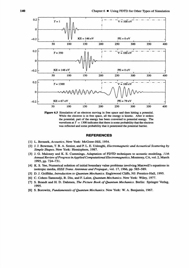
6.2.3 Simulation of an Electron Striking a Potential Barrier
139
(6.18)
(6.19)
Figure 6.3 shows a simulation of an electron moving in free space next to a region with
a potential of 100 eV. It is initiated at 146 eV, which is pure kinetic energy because there is
no potential. At 350 time steps, is has propagated to the right. The waveform has begun to
spread, but the total kinetic energy remains the same. After 1300 time steps, it has struck thepotential. Part of the waveformhas penetrated the potential barrier, and parthas been reflected.
Notice that the total energy has remained the same, but now part of it is in the form of potential
energy, because part of the waveform is at a potential of 100 eV. Does this mean the electron
has split into two parts? No. It means there is a certain probability that it has penetrated the
barrier and a certain probability that it has been reflected. These probabilities are calculated
by the following:
Probability of reflection =i: 1/F*(x)·1/F(x) dx (6.20a)
Probability of transmission =
1:1/F*(X)·1/F(X) dx, (6.20b)
where XPot. is the location where the potential begins. For this particular problem, Eq. (6.20a)
calculated 0.206 and Eq. (6.19b) calculated 0.794. Of course, the two must sum to one.
PROBLEM SET 6.2
1. The program se.c at the end of this section was used to do the simulation in Fig. 6.3. Get this
program running and duplicate the results.
2. Repeat the simulation of problem 6.2.1, but use a potential of -100 eV.
3. Repeat the simulation of problem 6.2.1 using a potential of 1000eVe
What happens? Does thismake sense?
8/7/2019 6_Using FDTD for Other Types of Simulation
http://slidepdf.com/reader/full/6using-fdtd-for-other-types-of-simulation 8/14
140 Chapter 6 • Using FDTD for Other Types of Simulation
4005000
PE=OeV
250
r - · _ · _ · _ · _ · _ _ · _ · _ · _ ·_ ·· V= lOOeV
I
20050
KE= 146eV
100
T= l
50
o. . . - - - - - - . .1-+,
0.2
-0.2
400500050
r - · _ · _ · _ · _ · - _ · _ · _ · _ · _ ·· V= lOOeV,
200SO00
T=350
50
0.. . ---------"
0.2
-0.2
r-·_·-·_·_·--·_·_·_·-·· V= lOOeV
I
T= 1300
ot------v:\. .1iJ-\
0.2
-0.2 KE=67 eV PE=7geV
50 100 150 200 250 300 350 400
Figure 6.3 Simulationof an electronmoving in free space and then hitting a potential.
While the electron is in free space, all the energy is kinetic. After it strikes
the potential, part of the energy has been convertedto potential energy. The
waveformat T =1300indicatesthatthere is someprobabilitythat theelectronwasreflectedand someprobabilitythatit penetratedthepotentialbarrier.
REFERENCES
[1] L. Beranek, Acoustics, New York: McGraw-Hill, 1954.
[2] J. J. Bowman, T. B. A. Senior, and P. L. E. Uslenghi, Electromagnetic andAcoustical Scattering by
Simple Shapes. New York: Hemisphere, 1987.
[3] J. G. Maloney and K. E. Cummings, Adaptation of FDTD techniques to acoustic modeling, 11th
AnnualReview ofProgress inAppliedComputational Electromagnetics,Monterey, CA, vol. 2,March
1995, pp. 724-731.[4] K. S. Vee, Numerical solution of initial boundary value problems involving Maxwell's equations in
isotropic media, IEEE Trans. Antennas and Propagat., vol. 17, 1966, pp. 585-589.
[5] D. J. Griffiths, Introduction to Quantum Mechanics. Englewood Cliffs, NJ: Prentice-Hall, 1995.
[6] C. Cohen-Tannoudji, B. Diu, and F. Laloe, QuantumMechanics. New York: Wiley, 1977.
[7] S. Brandt and H. D. Dahmen, The Picture Book ofQuantum Mechanics. Berlin: Springer Verlag,
1995.
[8] S. Borowitz, Fundamentals ofQuantum Mechanics. New York: W. A. Benjamin, 1967.
8/7/2019 6_Using FDTD for Other Types of Simulation
http://slidepdf.com/reader/full/6using-fdtd-for-other-types-of-simulation 9/14
C Programs 141
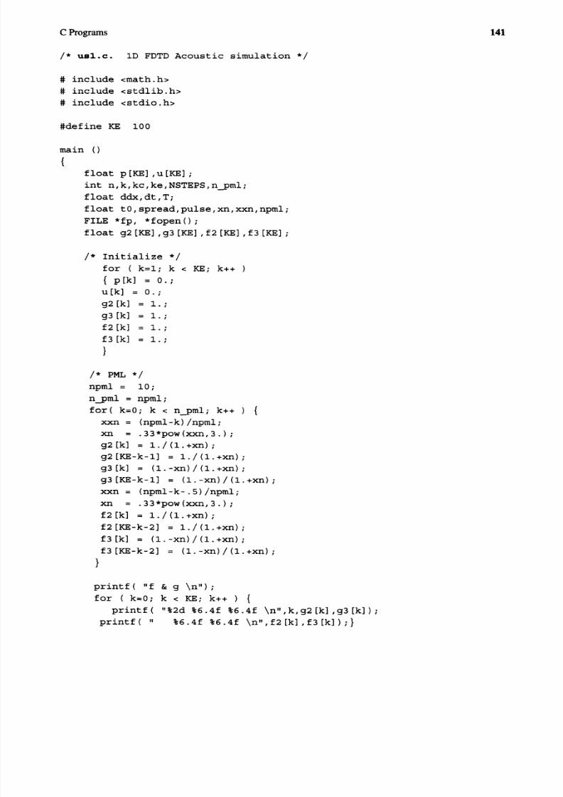
/* us l . c . 1D FDTD Acoustic s imu la ti on * /
# include <math.h>
# include <stdlib.h>
# i nc lude <stdio. h>
#define KE 100
main ()
{
f loa t p[KE] ,u[KE];
in t n,k,kc,ke,NSTEPS,n-pml;
f loa t ddx,dt,T;
f loat to,spread,pulse,xn,XXD,npml;
FILE *fp, *fopen(};
f loa t g2[KE] ,g3[KE] ,f2[KE] ,f3[KE];
/* In i t ia l ize */
for ( k=l; k < KE; k++ )
{ P [k ] = 0 . ;
u[k] = 0 .;
g2 [k ] 1 . i
g3 [k] 1 . ;
f2 [k ] 1 . i
f3 [k ] 1 . ;
}
/* PML */
npml = 10;
nJ>ml = npml;
fore k=O; k < n-pml; k++ ) {
xxn = (npml-k)/npml;
xn = .33*pow{xxn,3.) i
g2[k] = l . / ( l .+xn) ;
g2[KE-k-l] = 1./{1.+xn);
g3[k] = ( l . -xn)/{l .+xn);
g3[KE-k-l] = (1.-xn)/(1.+xn) ixxn = (npml-k-.S)/npmli
xn = .33*pow(xxn,3.);
f2[k] = 1. / ( l .+xn) i
f2[KE-k-2l = 1./(1.+xn);
f3[k] = ( l . -xn) /( l .+xn) ;
f3[KE-k-2] = ( l . -xn) /( l .+xn) ;
}
pr in t f ( Iff & 9 \n lf) i
for ( k=Oi k < KE; k++ ) {
pr in t f ( "%2d %6.4f %6.4f \n",k,g2[kl ,g3[k]) i
pr in t f ( If %6.4f %6.4f \n lf,f2[k],f3[k])i}
8/7/2019 6_Using FDTD for Other Types of Simulation
http://slidepdf.com/reader/full/6using-fdtd-for-other-types-of-simulation 10/14
142
kc = KE/2;
to = 150.0;
spread 50;
T = 0;
NSTEPS 1;
while ( NSTEPS > 0 ) {
pr in t f ( "NSTEPS - -> I I ) ;
scanf("%d", &NSTEPS);
printf("%d \n", NSTEPS);
n= 0;
for ( n=l; n <=NSTEPS n++)
{
T = T + 1;
/* Main FDTD Loop */
Chapter 6 • Using FDTD for Other Types of Simulation
/* Calcula te t he Pressure */
for ( k=l; k < KE; k++ )
{ P [k] 93 [k] *p [k] + 92 [k] *. (2 . 2SeS) * ( u [k-1] - u [k] )
/* Put a Gaussian pulse in the middle */
pulse = exp(-.S*(pow( (to-T)/spread,2.0) » ;
p[n-pml+S] = pulse;
pr in t f ( "%5.1f %6.2f\n",tO-T,p[nyml+S]);
/* Calcula te th e veloci ty */
for ( k=O; k < KE-l; k++ )
{ u [k] = f3 [k] *u [k] + f2 [k] * (6 . 67e- 8) * ( p [k] - P [k+l] )
/* End of the Main FDTD Loop */
/* At the end of the calculat ion, pr in t outthe pressure and veloci ty f ie ld s */
for ( k=1; k <= KE; k++ )
{ pr in t f ( "%3d %6.2f %6.2f\n",k,p[k],u[k]);
/* Write the P f ield out to a f i le "Pres" */
fp = fopen ( "Pres II , "w") ;
for ( k=l; k <= KE; k++ )
{ fpr in t f ( fp," %6.2f \n" ,p[k]) i
fclose(fp) ;
/* Write the U f ield out to a f i le "Vel" */
fp = fopen( "Vel II , "w") ;
for ( k=l; k <= KE; k++ )

8/7/2019 6_Using FDTD for Other Types of Simulation
http://slidepdf.com/reader/full/6using-fdtd-for-other-types-of-simulation 11/14
C Programs 143
{ fpr intf ( fp," %6.2f \n" ,u[k]) ; }
fclose (fp) ;
pr in t f ( liT = %5. Of\n" ,T) ;
8/7/2019 6_Using FDTD for Other Types of Simulation
http://slidepdf.com/reader/full/6using-fdtd-for-other-types-of-simulation 12/14
144 Chapter 6 • Using FDTD for Other Types of Simulation
/* se .c . 10 FOTO Schroedinger simulation */
# include <math.h>
# include <stdlib.h>
# i nc lude <stdio.h>
#define KE 400
main ()
{
f loa t psi_rl[KE] ,psi_im[KE] i
f loa t Vpot,vp[KE] i
in t n,k,kc,ke,kstart ,kcenter,NSTEPS,n-pml;
f loa t pi,melec,hbar;
f loa t lambda,sigma,ptot;
f loat ddx,dt , ra ,Ti
f loa t pulse,xn,xxn,npml;
FILE *fp, *fopen{);
f loa t lap_rl,lap_im,ke_rl,ke_im,kine,PE;
/* In i t ia l ize */
for ( k=Oi k < KE; k++ )
{ psi_rl[k] = 0 .;
psi_im[kl = 0 .;
vp [k] = 0 . ;
}
pi = 3.14159;
melec = 9.2e-31; /* Mass of an electron */
hbar = 1.0S5e-34; /* P lank's constant * /
ddx = .1e-lO; /* Cell s ize */
ra = 1 . /8 . ;
pr in t f ( "ra %e \n" , ra) ;
dt = .25* (melec/hbar)*pow{ddx,2.) ;
pr in t f ( " dt = %e \n" ,dt) i
printf{ " ks ta rt,Vpot ( in eV) --> I I ) ;
scanf{lI%d ",&kstart ) ;
scanf{"%f", &Vpot)i
for { k=kstart i k < KE; k++
{ vp[k] = Vpot*1.602e-19 ; /* Convert eV to Joules */
/* Write the Potent ia l to a f i le "Vpot" */
fp = fopen ( "Vpot", "w") ;
for ( k=O; k < KE; k++ )
{ fpr in t f ( fp," %6.2f \n",vp[kl*6.2415e18); /* Write in eV*/pr in t f (" %6.2f \n" , (d t /hbar)*vp[k]) ; }
fclose(fp);
8/7/2019 6_Using FDTD for Other Types of Simulation
http://slidepdf.com/reader/full/6using-fdtd-for-other-types-of-simulation 13/14
C Programs
/* In i t ia l ize the pulse */
pr in t f ( "lambda,sigma - -> ");
scanf("%f ",&lambda ) ;
scanf ( "%f" , &sigma);
kcenter = ksta r t /2 ;
pr in t f ( "kcenter = %3d \n lt, kcenter) ;
ptot = 0 .;
for ( k=l; k < ks tar t ; k++ )
{ psi_r l[kl = cos (2*pi* (k-kcenter)/lambda)
* exp( -.S*pow( (k-kcenter)/sigrna,2.) );
psi_im[kl = sin(2*pi*(k-kcenter) / lambda)
* exp( -.S*pow( (k-kcenter)/sigma,2.) );
ptot = ptot + pow(psi_rl[kl ,2.) + pow (psi_im[k] ,2 . ) ;
pr in t f ( " ptot= %f \n II , ptot) ;
/* Normalize the waveform */
for ( k=l; k < ks tar t ; k++ )
{ ps i_ rl [k l p si_ rl[k l/sq rt (p to t) ;
psi_im[kl = psi_im[kl /sqrt (ptot ) ;
kc = KE/2;
T = 0;
NSTEPS = 1;
while ( NSTEPS > 0 ) {
pr in t f ( "NSTEPS - -> I I ) ;
scanf ( II %d", &NSTEPS);
pr in t f ("%d \n", NSTEPS);
n= 0;
for ( n=l; n <=NSTEPS n++)
{
T = T + 1;
/* Main FDTD Loop */
/* Calc ula te th e Real part */
for { k=l; k < KE-l; k++
{ psi_rl[kJ = psi_rl[kJ
- ra*( psi_im[k+l] - 2.*psi_im[k] + psi_im[k-l] )
+ (dt/hbar)*vp[k]*psi_im[k] ; }
/* Calc ula te t he imaginary par t */
for ( k=l; k < KE-l; k++ )
{ psi_im[kJ = psi_im[kJ
+ ra*{ psi_rl[k+l] - 2.*psi_rl[k] + psi_r l [k- l ] )
145
8/7/2019 6_Using FDTD for Other Types of Simulation
http://slidepdf.com/reader/full/6using-fdtd-for-other-types-of-simulation 14/14
146 Chapter 6 • Using FDTD for Other Types of Simulation
- (dt/hbar)*vp[k] *psi_r l [k] ; }
/* End of the Main FDTD Loop */
/* Print out the rea land
imaginary par ts */for ( k=O; k < KE; k++ )
{ printf{ "%3d %6.2£ %6.2f\n",k,psi_rl[k] ,psi_im[k]);
/* Write the rea l pa rt to a f i le "prl" */
fp = fopen{ "pr l" , "w");
for ( k=O; k < KE; k++ )
{ fpr int f{ fp," %6.2f \n" ,ps i_r l [k] ) ;
fclose(fp) ;
/* Write the imaginary par t to a f i le "pim" */
fp = fopen ( "pim", "w") ;
for ( k=O; k < KE; k++ )
{ fprint£{ fp," %6.2f \n",psi_im[k]);
fclose{fp);
/* Calcula te th e KE and PE */
ke_rl = 0 .;
ke_im = O .i
PE = 0 .;
for { k=O; k < KE; k++ {
lap_rl = psi_r l[k+ll - 2.*psi_rl[k] + psi_r l[k- l ] ; /* Laplacian */
lap_im = psi_im[k+ll - 2.*psi_im[kl + psi_im[k-ll ;
ke_rl = ke_rl + psi_rl [k]*lap_rl + psi_im[kl*lap_im;
ke_im = ke_im + psi_rl[kl*lap_im - psi_im[kl*lap_rl;
PE = PE + vp[kl * {pow(psi_r l [kl ,2.) + pow{psi_im[k] , 2 . » ;
kine = .S*(hbar/melec)*(hbar/pow(ddx,2.»
*sqrt(pow(ke_rl ,2.) + pow(ke_im,2.»;
print f{ "k e %6.3f eV \n",6.23elS*kine); /* convert J to eV */print f{ " pe = %6.3f eV \n",6.23elS*PE);
pr in t f ( "T = %5.Of\n", T) ;
Related Documents


![FDTD Simulation of Exposure of Biological Material to ... · arXiv:physics/0407054v1 [physics.bio-ph] 12 Jul 2004 FDTD Simulation of Exposure of Biological Material to Electromagnetic](https://static.cupdf.com/doc/110x72/5ee1096fad6a402d666c1090/fdtd-simulation-of-exposure-of-biological-material-to-arxivphysics0407054v1.jpg)