6.241J Course Notes, Chapter 20: Stability robustness · Chapter 20 Stabilit y Robustness 20.1 In tro duction Last c hapter sho w ed ho the Nyquist stabilit y criterion pro vides

Lectures on Dynamic Systems and

Control

Mohammed Dahleh Munther A. Dahleh George Verghese

Department of Electrical Engineering and Computer Science

Massachuasetts Institute of Technology1

1�c

Chapter 20

Stability Robustness

20.1 Introduction

Last chapter showed how the Nyquist stability criterion provides conditions for the stability

robustness of a SISO system. It is possible to provide an extension of those conditions by gen-eralizing the Nyquist criterion for MIMO systems. This, however, turns out to be unnecessary

and a direct derivation is possible through the small gain theorem, which will be presented in

this chapter.

20.2 Additive Representation of Uncertainty

It is commonly the case that the nominal plant model is quite accurate for low frequencies

but deteriorates in the high-frequency range, because of parasitics, nonlinearities and/or time-varying e�ects that become signi�cant at higher frequencies. These high-frequency e�ects may

have been left unmodeled because the e�ort required for system identi�cation was not justi�ed

by the level of performance that was being sought, or they may be well-understood e�ects that

were omitted from the nominal model because they were awkward and unwieldy to carry along

during control design. This problem, namely the deterioration of nominal models at higher

frequencies, is mitigated to some extent by the fact that almost all physical systems have

strictly proper transfer functions, so that the system gain begins to roll o� at high frequency.

In the above situation, with a nominal plant model given by the proper rational matrix

P0(s), the actual plant represented by P (s), and the di�erence P (s) ; P0(s) assumed to be

stable, we may be able to characterize the model uncertainty via a bound of the form

�max

[P (j!) ; P0(j!)] � ` a(!) (20.1)

where (` a(!) �

\Small" � j!j � !c (20.2)\Bounded" � j!j � !c

This says that the response of the actual plant lies in a \band" of uncertainty around that of

the nominal plant. Notice that no phase information about the modeling error is incorporated

into this description. For this reason, it may lead to conservative results.

The preceding description suggests the following simple additive characterization of the

uncertainty set:

� � fP (s) j P (s) � P0(s) + W (s)�(s)g (20.3)

where � is an arbitrary stable transfer matrix satisfying the norm condition

k�k1

� sup �max(�(j!)) � 1 (20.4)

!

and the stable proper rational (matrix or scalar) weighting term W (s) is used to represent

any information we have on how the accuracy of the nominal plant model varies as a function

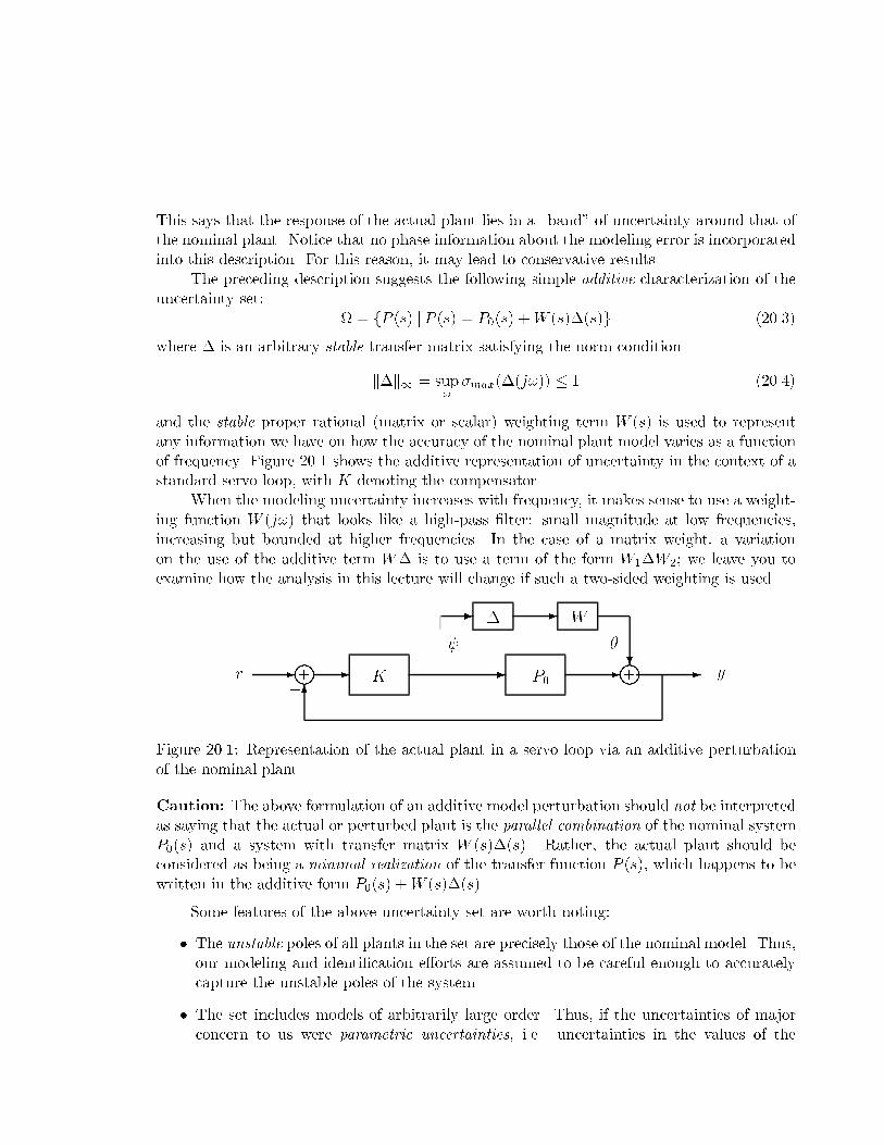
of frequency. Figure 20.1 shows the additive representation of uncertainty in the context of a

standard servo loop, with K denoting the compensator.

When the modeling uncertainty increases with frequency, it makes sense to use a weight-ing function W (j!) that looks like a high-pass �lter: small magnitude at low frequencies,

increasing but bounded at higher frequencies. In the case of a matrix weight, a variation

on the use of the additive term W � is to use a term of the form W1�W2� we leave you to

examine how the analysis in this lecture will change if such a two-sided weighting is used.

- -� W

� �

r

l+

- -. K

- P0

l+

-�

- y

; 6

Figure 20.1: Representation of the actual plant in a servo loop via an additive perturbation

of the nominal plant.

Caution: The above formulation of an additive model perturbation should not be interpreted

as saying that the actual or perturbed plant is the parallel combination of the nominal system

P0(s) and a system with transfer matrix W (s)�(s). Rather, the actual plant should be

considered as being a minimal realization of the transfer function P (s), which happens to be

written in the additive form P0(s) + W (s)�(s).

Some features of the above uncertainty set are worth noting:

� The unstable poles of all plants in the set are precisely those of the nominal model. Thus,

our modeling and identi�cation e�orts are assumed to be careful enough to accurately

capture the unstable poles of the system.

� The set includes models of arbitrarily large order. Thus, if the uncertainties of major

concern to us were parametric uncertainties, i.e. uncertainties in the values of the

parameters of a particular (e.g. state-space) model, then the above uncertainty set

would greatly overestimate the set of plants of interest to us.

The control design methods that we shall develop will produce controllers that are guar-anteed to work for every member of the plant uncertainty set. Stated slightly di�erently,

our methods will treat the system as though every model in the uncertainty set is a possible

representation of the plant. To the extent that not all members of the set are possible plant

models, our methods will be conservative.

20.3 Multiplicative Representation of Uncertainty

Another simple means of representing uncertainty that has some nice analytical properties is

the multiplicative perturbation, which can be written in the form

� � fP j P � P0(I + W �)� k�k1

� 1g: (20.5)

-- � W

� �

�

-. +m - P0

-

Figure 20.2: Representation of uncertainty as multiplicative perturbation at the plant input.

An alternative to this input-side representation of the uncertainty is the following output-side representation:

� � fP j P � (I + W �)P0� k�k1

� 1g: (20.6)

In both the multiplicative cases above, W and � are stable. As with the additive represen-tation, models of arbitrarily large order are included in the above sets. Still other variations

may be imagined� in the case of matrix weights, for instance, the term W � can be replaced

by W1�W2.

The caution mentioned in connection with the additive perturbation bears repeating

here: the above multiplicative characterizations should not be interpreted as saying that the

actual plant is the cascade combination of the nominal system P0

and a system I + W �.

Rather, the actual plant should be considered as being a minimal realization of the transfer

function P (s), which happens to be written in the multiplicative form.

Any unstable poles of P are poles of the nominal plant, but not necessarily the other

way, because unstable poles of P0

may be cancelled by zeros of I + W �. In other words,

the actual plant is allowed to have fewer unstable poles than the nominal plant, but all its

unstable poles are con�ned to the same locations as in the nominal model. In view of the

caution in the previous paragraph, such cancellations do not correspond to unstable hidden

modes, and are therefore not of concern.

20.4 More General Representation of Uncertainty

Consider a nominal interconnected system obtained by interconnecting various (reachable and

observable) nominal subsystems. In general, our representation of the uncertainty regarding

any nominal subsystem model such as P0

involves taking the signal � at the input or output

of the nominal subsystem, feeding it through an \uncertainty block" with transfer function

W � or W1�W2, where each factor is stable and k�k1

� 1, and then adding the output

� of this uncertainty block to either the input or output of the nominal subsystem. The

one additive and two multiplicative representations described earlier are special cases of this

construction, but the construction actually yields a total of three additional possibilities with

a given uncertainty block. Speci�cally, if the uncertainty block is W �, we get the following

additional feedback representations of uncertainty:

� P � P0(I ; W �P0);1�

� P � P0(I ; W �);1�

� P � (I ; W �);1P0.

A useful feature of the three uncertainty representations itemized above is that the unstable

poles of the actual plant P are not constrained to be (a subset of) those of the nominal plant

P0.

Note that in all six representations of the perturbed or actual system, the signals � and

� become internal to the actual subsystem model. This is because it is the combination of

P0

with the uncertainty model that constitutes the representation of the actual model P , and

the actual model is only accessed at its (overall) input and output.

In summary, then, perturbations of the above form can be used to represent many types of

uncertainty, for example: high-frequency unmodeled dynamics, unmodeled delays, unmodeled

sensor and/or actuator dynamics, small nonlinearities, parametric variations.

20.5 A Linear Fractional Description

We start with a given a nominal plant model P0, and a feedback controller K that stabilizes

P0. The robust stability question is then: under what conditions will the controller stabilize

all P 2 �� More generally, we assume we have an interconnected system that is nominally

internally stable, by which we mean that the transfer function from an input added in at

any subsystem input to the output observed at any subsystem output is always stable in

the nominal system. The robust stability question is then: under what conditions will the

interconnected system remain internally stable for all possible perturbed models.

If the plant uncertainty is speci�ed (additively, multiplicatively, or using a feedback

representation) via an uncertainty block of the form W �, where W and � are stable, then

the actual (closed-loop) system can be mapped into the very simple feedback con�guration

��

� �

-

G

w - z -

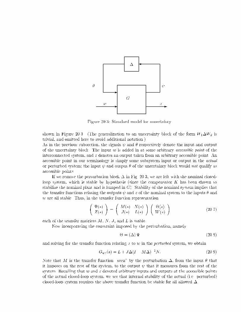
Figure 20.3: Standard model for uncertainty.

shown in Figure 20.3. (The generalization to an uncertainty block of the form W1�W2

is

trivial, and omitted here to avoid additional notation.)

As in the previous subsection, the signals � and � respectively denote the input and output

of the uncertainty block. The input w is added in at some arbitrary accessible point of the

interconnected system, and z denotes an output taken from an arbitrary accessible point. An

accessible point in our terminology is simply some subsystem input or output in the actual

or perturbed system� the input � and output � of the uncertainty block would not qualify as

accessible points.

If we remove the perturbation block � in Fig. 20.3, we are left with the nominal closed-loop system, which is stable by hypothesis (since the compensator K has been chosen to

stabilize the nominal plant and is lumped in G). Stability of the nominal system implies that

the transfer functions relating the outputs � and z of the nominal system to the inputs � and

w are all stable. Thus, in the transfer function representation � ! � ! � !

�(s) M(s) N(s) �(s)� (20.7)

Z(s) J(s) L(s) W (s)

each of the transfer matrices M , N , J , and L is stable.

Now incorporating the constraint imposed by the perturbation, namely

� � (�) � (20.8)

and solving for the transfer function relating z to w in the perturbed system, we obtain

Gwz(s) � L + J�(I ; M�);1N: (20.9)

Note that M is the transfer function \seen" by the perturbation �, from the input � that

it imposes on the rest of the system, to the output � that it measures from the rest of the

system. Recalling that w and z denoted arbitrary inputs and outputs at the accessible points

of the actual closed-loop system, we see that internal stability of the actual (i.e. perturbed)

closed-loop system requires the above transfer function be stable for all allowed �.

20.6 The Small-Gain Theorem

Since every term in Gwz

other than (I ;M�);1 is known to be stable, we shall have stability of

Gwz, and hence guaranteed stability of the actual closed-loop system, if (I ; M�);1 is stable

for all allowed �. In what follows, we will arrive at a condition | the small-gain condition

| that guarantees the stability of (I ; M�);1 . It can also be shown (see Appendix) that if

this condition is violated, then there is a stable � with k�k1

� 1 such that (I ; M�);1 and

�(I ; M�);1 are unstable, and Gwz

is unstable for some choice of z and w.

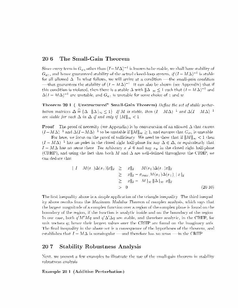
Theorem 20.1 (\Unstructured" Small-Gain Theorem) De�ne the set of stable pertur-4

bation matrices

6 � � f� j k�k1

� 1g. If M is stable, then (I ; M�);1 and �(I ; M�);1

are stable for each � in

6 � if and only if kMk1

� 1.

Proof. The proof of necessity (see Appendix) is by construction of an allowed � that causes

(I ;M�);1 and �(I ;M�);1 to be unstable if kMk1

� 1, and ensures that Gwz

is unstable.

For here, we focus on the proof of su�ciency. We need to show that if kMk1

� 1 then

(I ; M�);1 has no poles in the closed right half-plane for any � 2

6 �, or equivalently that

I ; M� has no zeros there. For arbitrary x 6� 0 and any s+

in the closed right half-plane

(CRHP), and using the fact that both M and � are well-de�ned throughout the CRHP, we

can deduce that

k[I ; M(s+)�(s+)]xk2

� kxk2

; kM(s+)�(s+)xk2

� kxk2

; �max[M(s+)�(s+)]k xk2

� kxk2

; kMk1

k�k1kxk2

� 0 (20.10)

The �rst inequality above is a simple application of the triangle inequality. The third inequal-ity above results from the Maximum Modulus Theorem of complex analysis, which says that

the largest magnitude of a complex function over a region of the complex plane is found on the

boundary of the region, if the function is analytic inside and on the boundary of the region.

In our case, both q0M 0Mq and q0�0�q are stable, and therefore analytic, in the CRHP, for

unit vectors q� hence their largest values over the CRHP are found on the imaginary axis.

The �nal inequality in the above set is a consequence of the hypotheses of the theorem, and

establishes that I ; M� is nonsingular | and therefore has no zeros | in the CRHP.

20.7 Stability Robustness Analysis

Next, we present a few examples to illustrate the use of the small-gain theorem in stability

robustness analysis.

Example 20.1 (Additive Perturbation)

For the con�guration in Figure 20.1, it is easily seen that

M � ;K(I + P0K);1W � ;(I + KP0);1KW

Example 20.2 (Multiplicative Perturbation)

A multiplicative perturbation of the form of Figure 20.2 can be inserted into the

closed-loop system at either the plant input or output. The procedure is then

identical to Example 20.1, except that M becomes a di�erent function. Again it

is easily veri�ed that for a multiplicative perturbation at the plant input,

M � ;(I + KP0);1KP0W� (20.11)

while a perturbation at the output yields

M � ;(I + P0K);1P0KW: (20.12)

What the above examples show is that stability robustness requires ensuring the weighted

versions of certain familiar transfer functions have H1

norms that are less than 1. For

instance, with a multiplicative perturbation at the output as in the last example, what we

require for stability robustness is kTW k1

� 1, where T is the complementary sensitivity

function associated with the nominal closed-loop system. This condition evidently has the

same �avor as the conditions we discussed earlier in connection with nominal performance of

the closed-loop system.

The small-gain theorem fails to take advantage of any special structure that there might

be in the uncertainty set

6 �, and can therefore be very conservative. As examples of the kinds

of situations that arise, consider the following two examples.

Example 20.3

Suppose we have a system that is best represented by the model of Figure 20.4.

When this system is reduced to the standard form, � will have a block-diagonal

Wa

- �a

�b

� Wb

66 � �

- +m - K

-. +m - P0

-+m -; 6

Figure 20.4: Plant with multiple uncertainties.

structure, since the two perturbations enter at di�erent points in the system: " #

�a

0

� � (20.13)0 �b

Thus, there is some added information about the plant uncertainty that can-not be captured by the unstructured small-gain theorem, and in general, even if

kMk1

� 1 for the M that corresponds to the � above, there may be no admissible

perturbation that will result in unstable (I ; M�);1 .

Example 20.4

Suppose that in addition to norm bounds on the uncertainty, we know that the

phase of the perturbation remains in the sector [;30�� 30�]. Again, even if kMk1

�

1 for the M that corresponds to the � for this system, there may be no admissible

perturbation that will result in unstable (I ; M�);1 .

In both of the preceding two examples, the unstructured small-gain theorem gives con-servative results.

Relating Stability Robustness to the (SISO) Nyquist Criterion

Suppose we have a SISO nominal plant with a multiplicative perturbation, and a nominally

stabilizing controller K. Then P � P0(1 + W �), and the compensated open-loop transfer

function is

PK � P0K + P0KW �: (20.14)

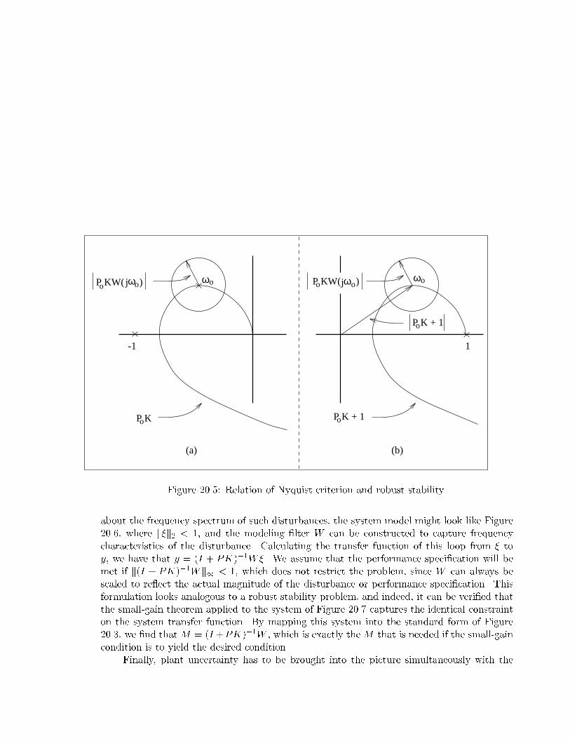
Since P0, K, and W are known and j�j � 1 with arbitrary phase, we may deduce from (20.14)

that the \real" Nyquist plot at any given frequency !0

is contained in a region delimited by

a circle centered at P0(j!0)K(j!0), with radius jP0KW (j!0)j. This is illustrated in Figure

20.5(a). Clearly, if the circle of uncertainty ever includes ;1, there is the possibility that the

\real" Nyquist plot has an extra encirclement, and hence is unstable. We may relate this

to the robust stability problem as follows. From Example 20.2, the SISO system is robustly

stable by the small gain theorem if ����

P0K

1 + P0K

W

����

� 1� 8 !: (20.15)

Equivalently,

jP0KW j � j1 + P0Kj: (20.16)

The right-hand side of (20.16) is the magnitude of a translation of the Nyquist plot of the

nominal loop transfer function. In Figure 20.5(b), because of the translation, encirclement

of zero will destabilize the system. Clearly, this cannot happen if (20.16) is satis�ed. This

makes the relationship of robust stability to the SISO Nyquist criterion clear.

Performance as Stability Robustness

Suppose that, for some plant model P , we wish to design a feedback controller that not only

stabilizes the plant (�rst order of priority!), but also provides some performance bene�ts, such

as improved output regulation in the presence of disturbances. Given that something is known

ωo ωojωjω

1

o oP K P K + 1

P K + 1

P KW( )

o

ooP KW( )o o

-1

(a) (b)

Figure 20.5: Relation of Nyquist criterion and robust stability.

about the frequency spectrum of such disturbances, the system model might look like Figure

20.6, where k�k2

� 1, and the modeling �lter W can be constructed to capture frequency

characteristics of the disturbance. Calculating the transfer function of this loop from � to

y, we have that y � (I + PK);1W�. We assume that the performance speci�cation will be

met if k(I + PK);1W k1

� 1, which does not restrict the problem, since W can always be

scaled to re�ect the actual magnitude of the disturbance or performance speci�cation. This

formulation looks analogous to a robust stability problem, and indeed, it can be veri�ed that

the small-gain theorem applied to the system of Figure 20.7 captures the identical constraint

on the system transfer function. By mapping this system into the standard form of Figure

20.3, we �nd that M � (I + PK);1W , which is exactly the M that is needed if the small-gain

condition is to yield the desired condition.

Finally, plant uncertainty has to be brought into the picture simultaneously with the

- - -

- - -

�

�

W

d�l+ +

Figure 20.6: Plant with disturbance.

�� �W

�

d

�

l6;

- -. K P

r y

l+ +

Figure 20.7: Mapping performance speci�cations into a stability problem.

performance constraints. This is necessary to formulate the performance robustness problem.

l6;

It should be evident that this will lead to situations with block-diagonal �, as was obtained

in the context of the last example in the previous subsection. The treatment of this case will

require the notion of structured singular values, as we shall see in the next lecture.

Appendix

Necessity of the small gain condition for robust stability can be proved by showing that if

�max[M(j!0)] � 1 for some !0, we can construct a � of norm less than one, such that the

resulting closed-loop map Gzv

is unstable. This is done as follows. Take the singular value

decomposition of M(j!0),

- - y. .K P

r

32

�1 64

75

�n

M(j!0) � U�V

0 � U V

0: (20.17)

. .

.

Since �max[M(j!0)] � 1, �1

� 1. Then �(j!0) can be constructed as: 32 66664

1��1

0 77775

�(j!0) � V U 0 (20.18). . .

0

Clearly, �max�(j!0) � 1. We then have 3232

�1

1��1 66664

�2

. . .

77775

V

0V

66664

0

. . .

77775

(I ; M�);1(j!0) � I ; U

0U

�n

0 22 33

1 66664

I ;

66664

77775

77775

0 0� U U (20.19). . .

0 32

� U

66664

0

1. . .

77775

0U

1

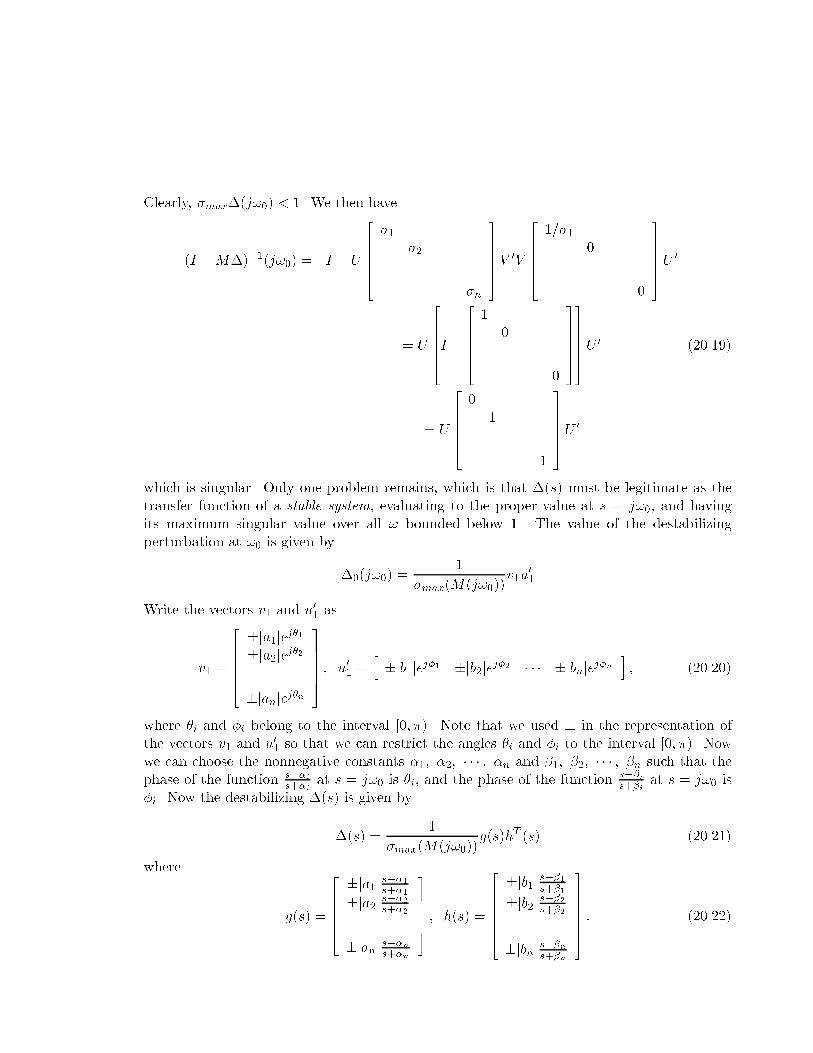
which is singular. Only one problem remains, which is that �(s) must be legitimate as the

transfer function of a stable system, evaluating to the proper value at s � j!0, and having

its maximum singular value over all ! bounded below 1. The value of the destabilizing

perturbation at !0

is given by

1 0�0(j!0) � v1u1�max(M(j!0))

Write the vectors v1

and u1

0 as 32 �ja1jej� 1

�ja2jej� 2

. . .

77775

v1

�

66664

ih 0

1

� �jb1jej�1 �jb2jej�2 � � � �jbnjej�n� u � (20.20)

�janjej� n

where �i

and �i

belong to the interval [0� �). Note that we used � in the representation of

the vectors v1

and u1

0 so that we can restrict the angles �i

and �i

to the interval [0� �). Now

we can choose the nonnegative constants �1� �2� � � � � �n

and �1� �2� � � � � �n

such that the

phase of the function

s;�i at s � j!0

is �i, and the phase of the function

s;�i at s � j!0

is s+�i

s+�i

�i. Now the destabilizing �(s) is given by

�(s) �

1

g(s)hT (s) (20.21)�max(M(j!0))

where 32 666664

�jb1j�jb j

s;�1

s+�1

s;�2

s+�2

777775

2 3 s;�1

s+�1�ja1j�ja j66664

77775

s;�2

s+�2

2 2

g(s) � � h(s) � : (20.22). .. .. .

�janj s;�n j s;�n

s+�n

�jbn s+�n

Exercises

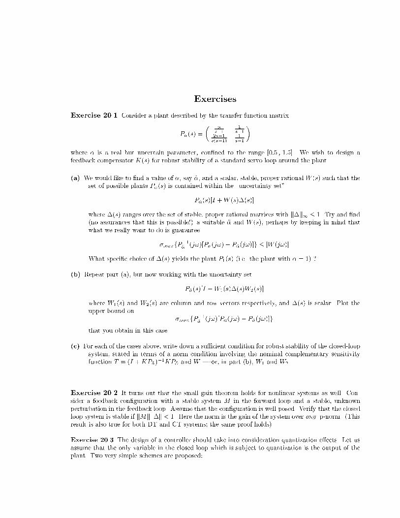
Exercise 20.1 Consider a plant described by the transfer function matrix � � 1

�

P�(s) �

s;1 s;1

2s;1 1

s(s;1) s;1

where � is a real but uncertain parameter, con�ned to the range [0:5 � 1:5]. We wish to design a

feedback compensator K(s) for robust stability of a standard servo loop around the plant.

(a) We would like to �nd a value of �, say �~ , and a scalar, stable, proper rational W (s) such that the

set of possible plants P�(s) is contained within the \uncertainty set"

P�~

(s)[I + W (s)�(s)]

where �(s) ranges over the set of stable, proper rational matrices with k�k1

� 1. Try and �nd

(no assurances that this is possible!) a suitable �~ and W (s), perhaps by keeping in mind that

what we really want to do is guarantee

�maxfP�~;

1(j!)[P�(j!) ; P�~

(j!)]g � jW (j!)j

What speci�c choice of �(s) yields the plant P1(s) (i.e. the plant with � � 1) �

(b) Repeat part (a), but now working with the uncertainty set

P�~

(s)[I + W1(s)�(s)W2

(s)]

where W1(s) and W2(s) are column and row vectors respectively, and �(s) is scalar. Plot the

upper bound on

�maxfP�;

1(j!)[P�(j!) ; P�~

(j!)]g~

that you obtain in this case.

(c) For each of the cases above, write down a su�cient condition for robust stability of the closed-loop

system, stated in terms of a norm condition involving the nominal complementary sensitivity

function T � (I + KP�~

);1KP�~

and W | or, in part (b), W1

and W2.

Exercise 20.2 It turns out that the small gain theorem holds for nonlinear systems as well. Con-sider a feedback con�guration with a stable system M in the forward loop and a stable, unknown

perturbation in the feedback loop. Assume that the con�guration is well-posed. Verify that the closed

loop system is stable if kMkk�k � 1. Here the norm is the gain of the system over any p-norm. (This

result is also true for both DT and CT systems� the same proof holds).

Exercise 20.3 The design of a controller should take into consideration quantization e�ects. Let us

assume that the only variable in the closed loop which is subject to quantization is the output of the

plant. Two very simple schemes are proposed:

- P0

K

� Q

�

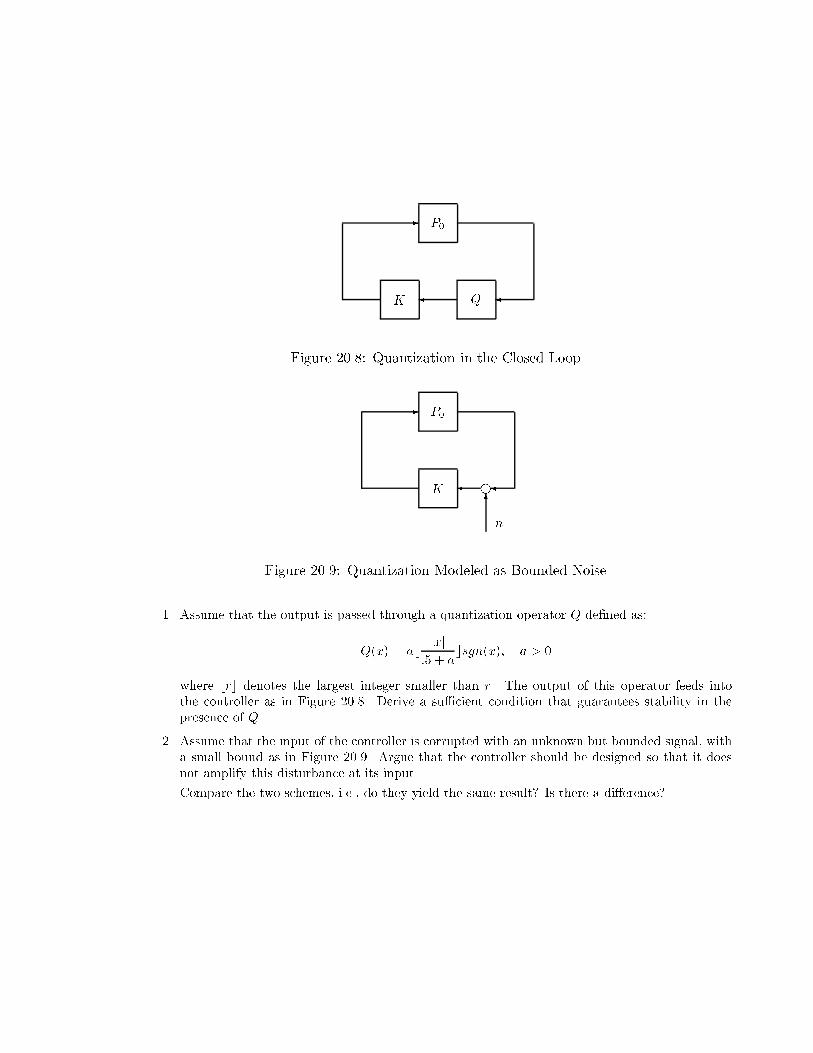
Figure 20.8: Quantization in the Closed Loop.

- P0

� f�K

6

n

Figure 20.9: Quantization Modeled as Bounded Noise.

1. Assume that the output is passed through a quantization operator Q de�ned as:

Q(x) � ab jxj csgn(x)� a � 0

:5 + a

where brc denotes the largest integer smaller than r. The output of this operator feeds into

the controller as in Figure 20.8. Derive a su�cient condition that guarantees stability in the

presence of Q.

2. Assume that the input of the controller is corrupted with an unknown but bounded signal, with

a small bound as in Figure 20.9. Argue that the controller should be designed so that it does

not amplify this disturbance at its input.

Compare the two schemes, i.e., do they yield the same result� Is there a di�erence�

MIT OpenCourseWarehttp://ocw.mit.edu

6.241J / 16.338J Dynamic Systems and Control Spring 2011

For information about citing these materials or our Terms of Use, visit: http://ocw.mit.edu/terms.