6 Parametrization and Vector Fields - Jay Daigle

Jay Daigle Occidental College Math 212: Multivariable Calculus

6 Parametrization and Vector Fields

So far in this course we’ve discussed two types of functions. Single-variable functions are

the ones you’re familiar with from single-variable calculus; multi-variable functions, like the

ones we’ve been studying, take in multiple variables, but output one.

However, we can also have functions that output more than one variables. In this section

we will lay out various types of functions that output multiple variables, and talk about

what situationst hey are used to describe. In future sections we will apply calculus ideas to

them.

6.1 Curves and Motion

In this section we want to study curves through space. By a curve we mean, essentially,

any shape that is in some sense “one-dimensional”. So a line, a circle, and a curving spiral

through three-dimensional space are all curves.

The essence of a curve is the one-dimensionality. We capture this idea by requiring

position on our curves to be described by one single real number. That is, we can describe

our position on the curve with exactly one coordinate. We say a system of coordinates

for an object is a “parametrization”, because it describes the object with some number of

parameters.

Definition 6.1. We say a function ~r : R→ Rn is a parametrization of a curve.

Sometimes we want to consider the components of the function. We will usually write

~r(t) = (x(t), y(t), z(t)) and say that the single-variable functions x(t), y(t), z(t) are the com-

ponents of ~r.

Example 6.2. Let’s find a parametrization for the curve y = x2.

We see that we can parametrize this by the function ~r(t) = (t, t2). You’ll notice that this

is basically the original function formula: we have x = t and y = t2 = x2. Any time we have

a curve that is the graph of a function, we effectively have a parametrization for free; the

input variable gives us a parametrization.

Example 6.3. Let’s parametrize a circle of radius 1. Notice that we can’t use the same

trick as last time, since this isn’t a function.

We could try something like x(t) = t, y(t) =√

1− t2 for −1 ≤ t ≤ 1. This sort of works,

but only captures the top half of the circle. We could keep trying to make this idea work,

but it baically won’t.

http://jaydaigle.net/teaching/courses/2018-spring-212/ 76

http://jaydaigle.net/teaching/courses/2018-spring-212/


Instead, we take advantage of the fact that circles are fundamentally trigonometric. We

see that ~r(t) = (cos(t), sin(t)) will give us every point on the circle—in fact, this is the usual

unit circle definition of sin and cos. In particular, we have ~r(0) = (1, 0) is the rightmost

point of the circle, and as t increases we move counterclockwise around the circle.

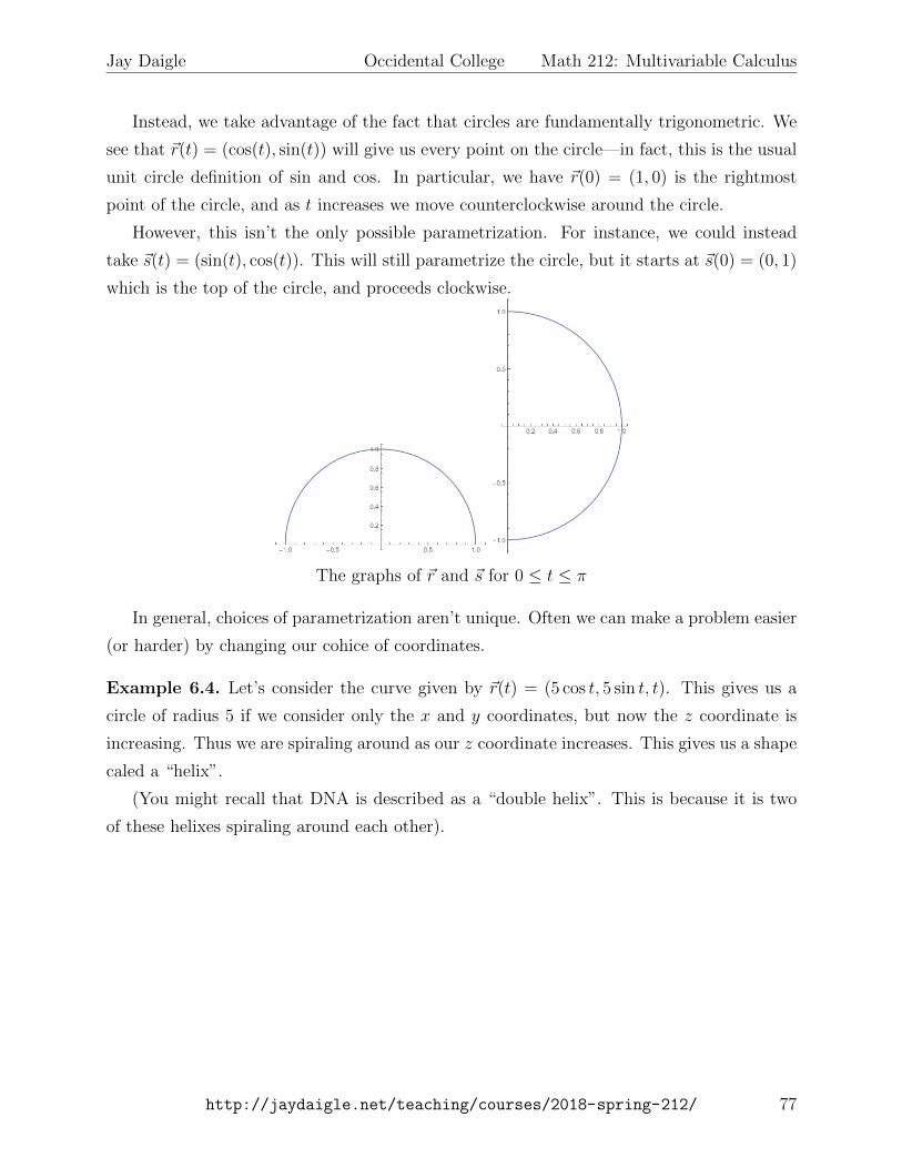
However, this isn’t the only possible parametrization. For instance, we could instead

take ~s(t) = (sin(t), cos(t)). This will still parametrize the circle, but it starts at ~s(0) = (0, 1)

which is the top of the circle, and proceeds clockwise.

The graphs of ~r and ~s for 0 ≤ t ≤ π

In general, choices of parametrization aren’t unique. Often we can make a problem easier

(or harder) by changing our cohice of coordinates.

Example 6.4. Let’s consider the curve given by ~r(t) = (5 cos t, 5 sin t, t). This gives us a

circle of radius 5 if we consider only the x and y coordinates, but now the z coordinate is

increasing. Thus we are spiraling around as our z coordinate increases. This gives us a shape

caled a “helix”.

(You might recall that DNA is described as a “double helix”. This is because it is two

of these helixes spiraling around each other).




The two most common shapes to parametrize are probably circles and lines. We’ve looked

at circles already; now let’s consider lines.

Example 6.5. Let’s parametrize the line through (1, 3, 5) in the direction of 2~i−~j + 3~k.

This is simple and straightforward. We get ~r(t) = (1, 3, 5) + t(2,−1, 3) = (1 + 2t, 3 −t, 5 + 3t)

In general, a line is described by a point and a direction. Therefore, if we want to

parametrize a line, we can use the equation ~r(t) = ~r0 + t~v where ~r0 is the known point and

~v is the direction.

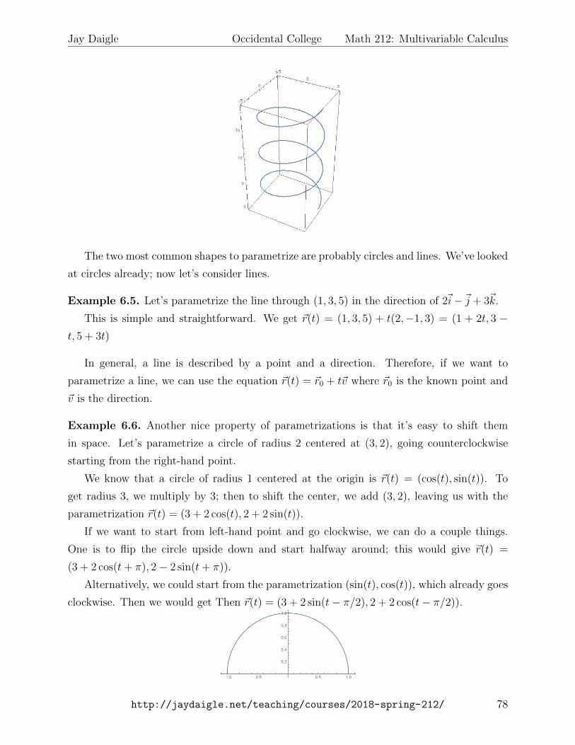
Example 6.6. Another nice property of parametrizations is that it’s easy to shift them

in space. Let’s parametrize a circle of radius 2 centered at (3, 2), going counterclockwise

starting from the right-hand point.

We know that a circle of radius 1 centered at the origin is ~r(t) = (cos(t), sin(t)). To

get radius 3, we multiply by 3; then to shift the center, we add (3, 2), leaving us with the

parametrization ~r(t) = (3 + 2 cos(t), 2 + 2 sin(t)).

If we want to start from left-hand point and go clockwise, we can do a couple things.

One is to flip the circle upside down and start halfway around; this would give ~r(t) =

(3 + 2 cos(t+ π), 2− 2 sin(t+ π)).

Alternatively, we could start from the parametrization (sin(t), cos(t)), which already goes

clockwise. Then we would get Then ~r(t) = (3 + 2 sin(t− π/2), 2 + 2 cos(t− π/2)).




We can use parametrizations of curves to find where they intersect surfaces.

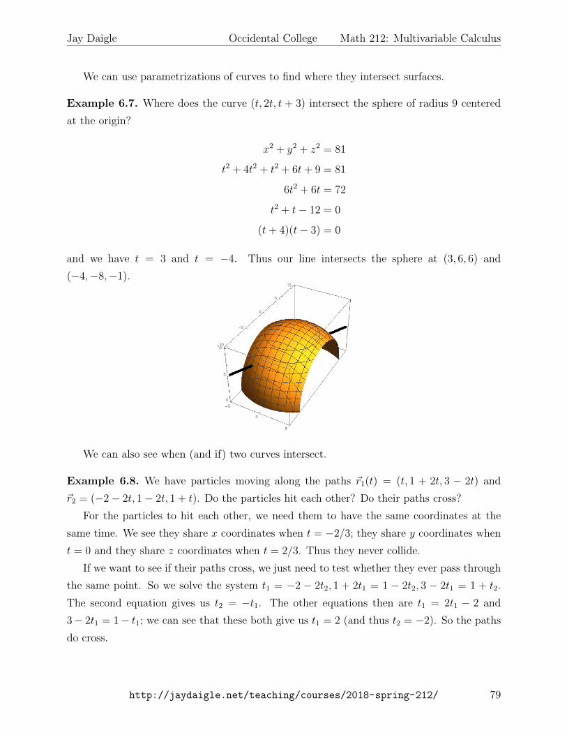
Example 6.7. Where does the curve (t, 2t, t + 3) intersect the sphere of radius 9 centered

at the origin?

x2 + y2 + z2 = 81

t2 + 4t2 + t2 + 6t+ 9 = 81

6t2 + 6t = 72

t2 + t− 12 = 0

(t+ 4)(t− 3) = 0

and we have t = 3 and t = −4. Thus our line intersects the sphere at (3, 6, 6) and

(−4,−8,−1).

We can also see when (and if) two curves intersect.

Example 6.8. We have particles moving along the paths ~r1(t) = (t, 1 + 2t, 3 − 2t) and

~r2 = (−2− 2t, 1− 2t, 1 + t). Do the particles hit each other? Do their paths cross?

For the particles to hit each other, we need them to have the same coordinates at the

same time. We see they share x coordinates when t = −2/3; they share y coordinates when

t = 0 and they share z coordinates when t = 2/3. Thus they never collide.

If we want to see if their paths cross, we just need to test whether they ever pass through

the same point. So we solve the system t1 = −2 − 2t2, 1 + 2t1 = 1 − 2t2, 3 − 2t1 = 1 + t2.

The second equation gives us t2 = −t1. The other equations then are t1 = 2t1 − 2 and

3− 2t1 = 1− t1; we can see that these both give us t1 = 2 (and thus t2 = −2). So the paths

do cross.




Remark 6.9. Here we have three equations in two variables, so it’s very easy for the paths

not to cross. But it’s also quite possible for them to cross in two or more points.

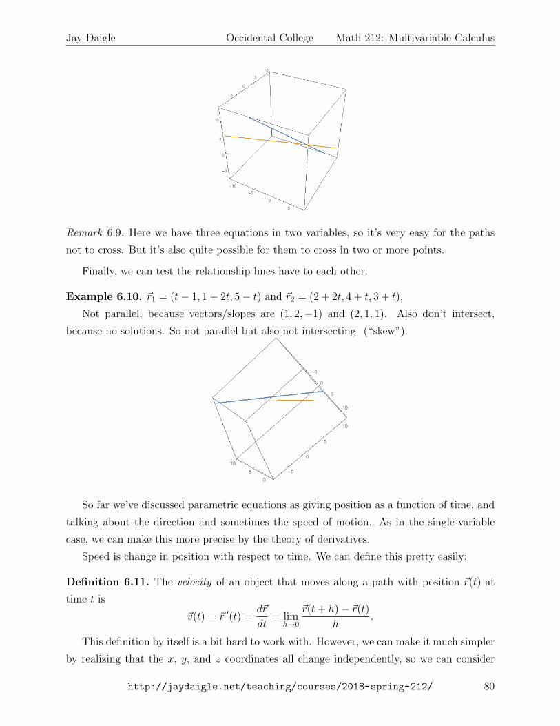
Finally, we can test the relationship lines have to each other.

Example 6.10. ~r1 = (t− 1, 1 + 2t, 5− t) and ~r2 = (2 + 2t, 4 + t, 3 + t).

Not parallel, because vectors/slopes are (1, 2,−1) and (2, 1, 1). Also don’t intersect,

because no solutions. So not parallel but also not intersecting. (“skew”).

So far we’ve discussed parametric equations as giving position as a function of time, and

talking about the direction and sometimes the speed of motion. As in the single-variable

case, we can make this more precise by the theory of derivatives.

Speed is change in position with respect to time. We can define this pretty easily:

Definition 6.11. The velocity of an object that moves along a path with position ~r(t) at

time t is

~v(t) = ~r ′(t) =d~r

dt= lim

h→0

~r(t+ h)− ~r(t)h

.

This definition by itself is a bit hard to work with. However, we can make it much simpler

by realizing that the x, y, and z coordinates all change independently, so we can consider




them independently. (This is implicitly because derivatives are always linear, so we can write

the derivative of a sum as the sum of the derivatives).

Proposition 6.12. Let ~r : R2 → R3 be a differentiable function. Then

~r ′(t) = (x′(t), y′(t), z′(t)).

Proof.

~r ′(t) = limh→0

~r(t+ h)− ~r(t)h

= limh→0

x(t+ h)~i+ y(t+ h)~j + z(t+ h)~k − x(t)~i− y(t)~j − z(t)~k

h

= limh→0

x(t+ h)− x(t)

h~iy(t+ h)− y(t)

h~j +

z(t+ h)− z(t)

h~k

= x′(t)~i+ y′(t)~j + z′(t)~k.

Example 6.13. Consider the circle parametrized by (cos(t), sin(t)). Then the derivative is

~r ′(t) = (− sin(t), cos(t)).

If we want to find the tangent vector at the point (1, 0), we compute the derivative and

plug in t = 0, so we get ~r ′(0) = (0, 1) as your vector, and the tangent line is (1, 0 + t).

Now suppose want the tangent line at (√

2/2,√

2/2). This occurs at time t = π/4 and

so we compute ~r ′(π/4) = (−√

2/2,√

2/2). Thus the tangent line is√

2/2(1− t, 1 + t).

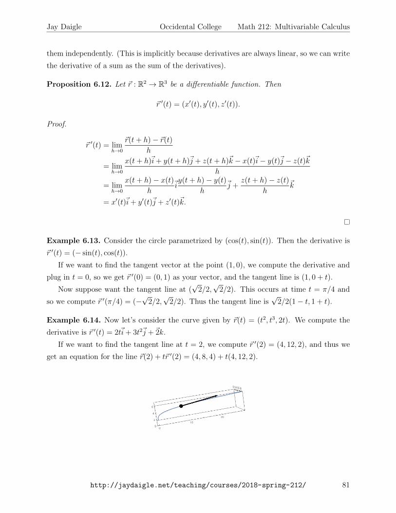
Example 6.14. Now let’s consider the curve given by ~r(t) = (t2, t3, 2t). We compute the

derivative is ~r ′(t) = 2t~i+ 3t2~j +~2k.

If we want to find the tangent line at t = 2, we compute ~r ′(2) = (4, 12, 2), and thus we

get an equation for the line ~r(2) + t~r ′(2) = (4, 8, 4) + t(4, 12, 2).




After taking the first derivative, we can also take the second (and further) derivatives.

As in the single variable case, if the function gives position, and the derivative gives velocity,

then the second derivative gives acceleration.

Definition 6.15. The acceleration of an object that moves along a path with position ~r(t)

at time t is

~a(t) = ~v ′(t) = ~r ′′(t) =d2~r

dt2= lim

h→0

~r ′(t+ h)− ~r ′(t)h

.

As you’d expect, we can compute the acceleration just by taking the componentwise

second derivatives: we have

~a(t) = ~v ′(t) = ~r ′′(t) = (x′′(t), y′′(t), z′′(t)).

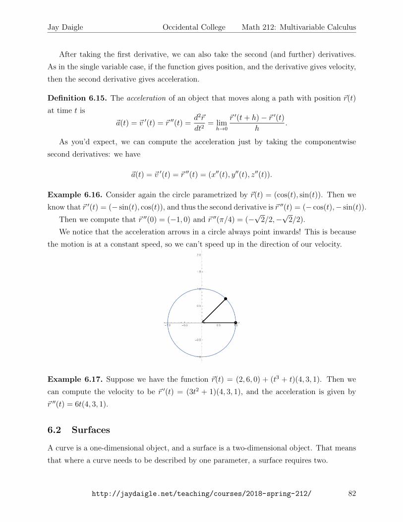
Example 6.16. Consider again the circle parametrized by ~r(t) = (cos(t), sin(t)). Then we

know that ~r ′(t) = (− sin(t), cos(t)), and thus the second derivative is ~r ′′(t) = (− cos(t),− sin(t)).

Then we compute that ~r ′′(0) = (−1, 0) and ~r ′′(π/4) = (−√

2/2,−√

2/2).

We notice that the acceleration arrows in a circle always point inwards! This is because

the motion is at a constant speed, so we can’t speed up in the direction of our velocity.

Example 6.17. Suppose we have the function ~r(t) = (2, 6, 0) + (t3 + t)(4, 3, 1). Then we

can compute the velocity to be ~r ′(t) = (3t2 + 1)(4, 3, 1), and the acceleration is given by

~r ′′(t) = 6t(4, 3, 1).

6.2 Surfaces

A curve is a one-dimensional object, and a surface is a two-dimensional object. That means

that where a curve needs to be described by one parameter, a surface requires two.




Definition 6.18. A parametrization of a surface is a function ~r : R2 → Rn.

Sometimes write in components: ~r(s, t) = (x(s, t), y(s, t), z(s, t)). Each component is a

multivariable function R2 → R.

We’ve already seen some very important examples.

Example 6.19. The graph of a function z = f(x, y) is given by the parametrization ~r(s, t) =

(s, t, f(s, t)).

Parametrizations and coordinate systems are the same idea—describing a point with a

collection of numbers. Thus the alternate coordinate systems we’ve seen can be viewed as

parametrizations.

Example 6.20. We can parametrize a sphere using spherical coordinates. A sphere of radius

5 is parametrized by ~r(θ, φ) = (5 sinφ cos θ, 5 sinφ sin θ, 5 cosφ).

Example 6.21. Let’s parametrize a cylinder of radius 1, centered at the origin. We can

do this, effectively, with cylindrical coordinates. We have the parametrization ~r(θ, z) =

(cos(θ), sin(θ), z).

If we want to parametrize a cylinder of radius 3 centered at the line y = 3, z = −4, then

we just need to tweak this. Notice that this cylinder is pointing in a new direction! We get

~r(θ, s) = (s, 3 cos(θ) + 3, 3 sin(θ)− 4).

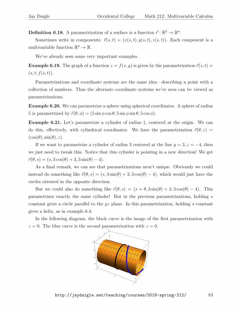
As a final remark, we can see that parametrizations aren’t unique. Obviously we could

instead do something like ~r(θ, s) = (s, 3 sin(θ) + 3, 3 cos(θ) − 4), which would just have the

circles oriented in the opposite direction.

But we could also do something like ~r(θ, s) = (s + θ, 3 sin(θ) + 3, 3 cos(θ) − 4). This

parametrizes exactly the same cylinder! But in the previous parametrizations, holding s

constant gives a circle parallel to the yz plane. In this parametrization, holding s constant

gives a helix, as in example 6.4.

In the following diagram, the black curve is the image of the first parametrization with

z = 0. The blue curve is the second parametrization with z = 0.




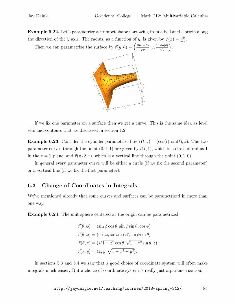
Example 6.22. Let’s parametrize a trumpet shape narrowing from a bell at the origin along

the direction of the y axis. The radius, as a function of y, is given by f(x) = 10√x.

Then we can parametrize the surface by ~r(y, θ) =(

10 cos(θ)√y

, y, 10 sin(θ)√y

).

If we fix one parameter on a surface then we get a curve. This is the same idea as level

sets and contours that we discussed in section 1.2.

Example 6.23. Consider the cylinder parametrized by ~r(t, z) = (cos(t), sin(t), z). The two

parameter curves through the point (0, 1, 1) are given by ~r(t, 1), which is a circle of radius 1

in the z = 1 plane; and ~r(π/2, z), which is a vertical line through the point (0, 1, 0).

In general every parameter curve will be either a circle (if we fix the second parameter)

or a vertical line (if we fix the first parameter).

6.3 Change of Coordinates in Integrals

We’ve mentioned already that some curves and surfaces can be parametrized in more than

one way.

Example 6.24. The unit sphere centered at the origin can be parametrized:

~r(θ, φ) = (sinφ cos θ, sinφ sin θ, cosφ)

~r(θ, φ) = (cosφ, sinφ cos θ, sinφ sin θ)

~r(θ, z) = (√

1− z2 cos θ,√

1− z2 sin θ, z)

~r(x, y) = (x, y,√

1− x2 − y2).

In sections 5.3 and 5.4 we saw that a good choice of coordinate system will often make

integrals much easier. But a choice of coordinate system is really just a parametrization.




Example 6.25. Let’s parametrize the xy plane. We can parametrize this:

~r(s, t) = (s, t)

~r(s, t) = (t, s)

~r(s, t) = (3s, s− t)

~r(s, t) = (s cos t, s sin t).

This last parametrization is just polar coordinates.

Remark 6.26. This is the same idea as “change of basis” in a linear algebra context.

In general, we can use customized parametrizations to make double integrals easier. If

we have a parametrization given by ~r(s, t) = (x(s, t), y(s, t)), this means we’ll divide our

region up into rectangles in (s, t) coordinates, and sum up the values in each rectangle. To

make this useful, we need to figure out how area in (s, t)-coordinates relates to area in (x, y)

coordinates.

Suppose we have a a small rectangle in (s, t) coordinates, with corners at

(s, t), (s+ ∆s, t), (s, t+ ∆t), (s+ ∆s, t+ ∆t).

Then its image under the ~r transformation is going to be some four-sided shape with curved

sides, with corners at the points

(x(s, t), y(s, t)), (x(s+∆s, t), y(s+∆s, t)), (x(s, t+∆t), y(s, t+∆t)), (x(s+∆s, t+∆t), y(s+∆s, t+∆t)).

When ∆s,∆t are small, we can treat this as a parallelogram. So we just need to find the

area of a parallelogram.

You might recall from section 2.4 proposition 2.39 that the area of a parallelogram with

sides given by the vectors ~u and ~v is ‖~u × ~v‖. So we need to figure out the vectors for the

sides of this parallelogram.

But since these vectors are just ∆x∆s~i+ ∆y

∆s~j and ∆x

∆t~i+ ∆y

∆t~j, we can approximate these with

directional derivatives. In particular, when the sides are small, they are approximately given

by ∂x∂s

∆s~i+ ∂y∂s~j and ∂x

∂t∆t~i+ ∂y

∂t∆t~j. Thus the area of the parallelogram is approximately∣∣∣∣(∂x∂s∆s~i+

∂y

∂s~j

)×(∂x

∂t∆t~i+

∂y

∂t∆t~j

)∣∣∣∣ =

∣∣∣∣∂x∂s∆s∂y

∂t∆t− ∂x

∂t∆t∂y

∂s∆s

∣∣∣∣=

∣∣∣∣∂x∂s ∂y∂d − ∂x

∂t

∂y

∂s

∣∣∣∣∆s∆t.http://jaydaigle.net/teaching/courses/2018-spring-212/ 85



Definition 6.27. We define the Jacobian of a function to be the determinant of the matrix

of partial derivatives. Thus the Jacobian of ~r : R2 → R2 is

∂(x, y)

∂(s, t)=∂x

∂s

∂y

∂t− ∂x

∂t

∂y

∂s=

∣∣∣∣∣∂x∂s ∂x∂t

∂y∂s

∂y∂t

∣∣∣∣∣ .Thus the area of the parallelogram we’re studying is approximately

∣∣∣∂(x,y)∂(s,t)

∣∣∣∆s∆t.So now let’s return to thinking about our integral. If we want to compute an integral,

we have the following computation:∫r

f(x, y) dA = lim∑

f(u∗ij, v∗ij)

∣∣∣∣∂(x, y)

∂(s, t)

∣∣∣∣∆s∆t= lim

∑f(x(s∗ij, t

∗ij), y(s∗ij, t

∗ij))

∣∣∣∣∂(x, y)

∂(s, t)

∣∣∣∣∆s∆t=

∫T

f(x(s, t), y(s, t))

∣∣∣∣∂(x, y)

∂(s, t)

∣∣∣∣ ds dt.Thus in summary, we can compute integrals in a new coordinate system by doing the

following:

1. Substitue x(s, t) and y(s, t) for x and y in the inside of the integral.

2. Change the region/bounds to be described in terms of s and t.

3. Make the substitution dx dy =∣∣∣∂(x,y)∂(s,t)

∣∣∣ ds dt.Remark 6.28. This is a generalization of u-substitution in single-variable calculus. Recall

there that if x = g(u) then ∫ b

a

f(g(u))g′(u) du =

∫ g(b)

g(a)

f(x) dx.

Just as in this reparametrization, we do a substitution inside the variable; we change the

bounds; and we have a correcting factor from the derivative of x = g(u).

Example 6.29. We can recover polar coordinates from this setup. Polar coordinates give

the parametrization x = r cos θ, y = r sin θ. Then we compute

∂(x, y)

∂(r, θ)=

∣∣∣∣∣∂x∂r ∂x∂θ

∂y∂r

∂y∂θ

∣∣∣∣∣ =

∣∣∣∣∣cos θ −r sin θ

sin θ r cos θ

∣∣∣∣∣ = r cos2 θ + r sin2 θ = r.

This gives us back exactly the conversion factor that we got before.




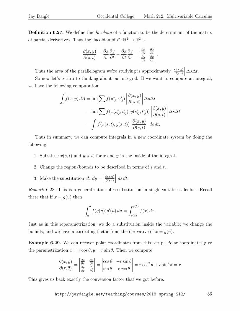
Example 6.30. Let’s find the area of an ellipse given by the equation x2/a2 + y2/b2 = 1.

We can parametrize this with x = as, y = bt. Then the equation becomes s2 + t2 = 1, so

the region is the unit circle in the st plane. We calculate the Jacobian is

∣∣∣∣∣a 0

0 b

∣∣∣∣∣ = ab. Thus

the area of the ellipse is∫R

1 dx dy =

∫T

1ab ds dt = ab

∫T

1 ds dt = abπ.

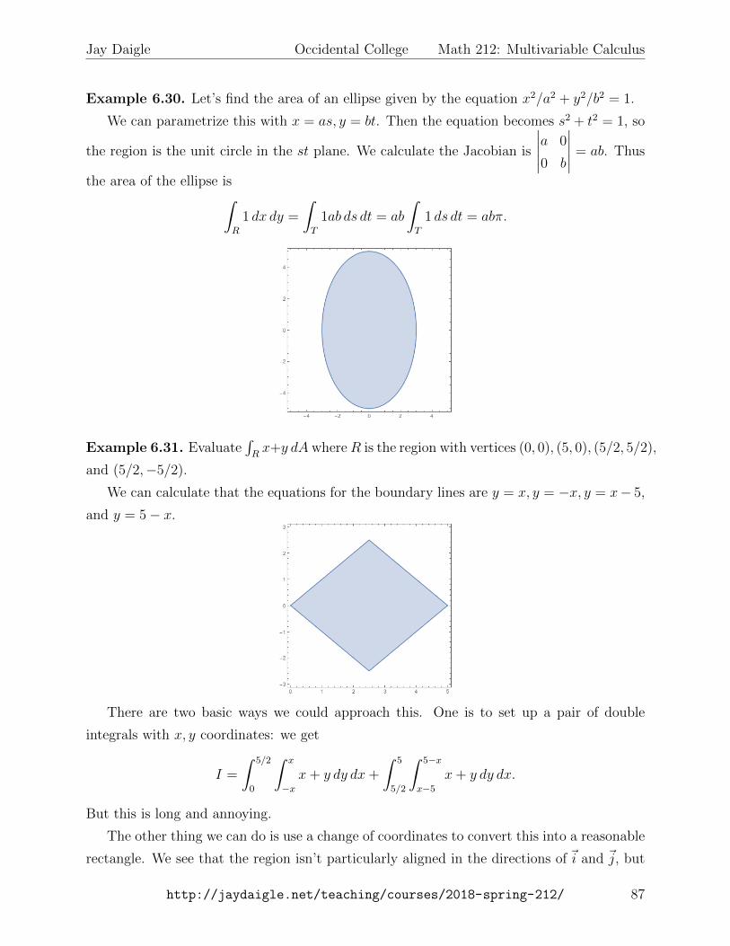
Example 6.31. Evaluate∫Rx+y dA whereR is the region with vertices (0, 0), (5, 0), (5/2, 5/2),

and (5/2,−5/2).

We can calculate that the equations for the boundary lines are y = x, y = −x, y = x− 5,

and y = 5− x.

There are two basic ways we could approach this. One is to set up a pair of double

integrals with x, y coordinates: we get

I =

∫ 5/2

0

∫ x

−xx+ y dy dx+

∫ 5

5/2

∫ 5−x

x−5

x+ y dy dx.

But this is long and annoying.

The other thing we can do is use a change of coordinates to convert this into a reasonable

rectangle. We see that the region isn’t particularly aligned in the directions of ~i and ~j, but




rather in the directions ~i + ~j and ~i − ~j. So we might try a parametrization x = s + t and

y = s− t.To find our new bounds we plug this into our boundary equations. For y = x we get

s− t = s+ t, which gives us t = 0. For y = −x we get s− t = −s− t, which gives us s = 0.

Similarly, for y = x− 5 we get s− t = s+ t− 5. Solving gives t = 5/2. Finally, we have

y = 5− x, which gives s− t = 5− s− t, which gives s = 5/2.

Thus, rather than having a complicated integral setup, we just get bounds 0 ≤ s ≤5/2, 0 ≤ t ≤ 5/2. Our integrand is x+ y = s+ t+ s− t = 2s. And our Jacobian is∣∣∣∣∣1 1

1 −1

∣∣∣∣∣ = | − 1− 1| = 2.

Thus we have the integral

I =

∫ 5/2

0

∫ 5/2

0

2s · 2 dt ds

=

∫ 5/2

0

4st|5/20 ds =

∫ 5/2

0

10s ds

= 5s2|5/20 =125

4.

Example 6.32. We can also generalize this to three variables. Spherical coordinates are

given by the transformation x = ρ sinφ cos θ, y = ρ sinφ sin θ, z = ρ cosφ. Then we compute

the Jacobian is∣∣∣∣∣∣∣∣∂x∂ρ

∂x∂θ

∂x∂φ

∂y∂ρ

∂y∂θ

∂y∂φ

∂z∂ρ

∂z∂θ

∂z∂φ

∣∣∣∣∣∣∣∣ =

∣∣∣∣∣∣∣∣sinφ cos θ −ρ sinφ sin θ ρ cosφ cos θ

sinφ sin θ ρ sinφ cos θ ρ cosφ sin θ

cosφ 0 −ρ sinφ

∣∣∣∣∣∣∣∣= | − ρ2 sin3 φ cos2 θ − ρ2 sin2 θ sinφ cos2 φ

− ρ2 sinφ cos2 φ cos2 θ − ρ2 sin3 φ sin2 θ|

= ρ2∣∣sin3 φ(cos2 θ + sin2 θ) + sinφ cos2 φ(sin2 θ + cos2 θ)

∣∣= ρ2

∣∣sin2 φ(sinφ+ cos2 φ)∣∣

= ρ2| sinφ| = ρ2 sinφ.

(We can drop the absolute values around sin because sinφ ≥ 0 when φ ∈ [0, π]).

6.4 Vector Fields

In subsection 6.1 we talked about curves, which are functions ~r : R→ R3. In subsection 6.2

we talked about surfaces, which are functions ~r : R2 → R3. Now we’ll discuss vector fields,




which are functions ~F : R3 → R3. (Or, more generally, functions ~F : Rn → Rn).

The basic idea is that sometimes we have a flow, or a force field, or a current. What these

all have in common is that for every point they have a direction and a magnitude, which

represents the flow of the current, or the force of the force field. Thus we want to write a

function that takes in a location, which is a point in R3, and outputs a vector in R3.

Example 6.33. � The current direction and distance you have to go to reach your des-

tination.

� The force exerted by the Earth’s gravitic force.

� The direction and speed of the currents in a river.

Definition 6.34. A vector field in Rn is a function F : Rn → Rn that takes in a point in Rn

and outputs a vector in Rn.

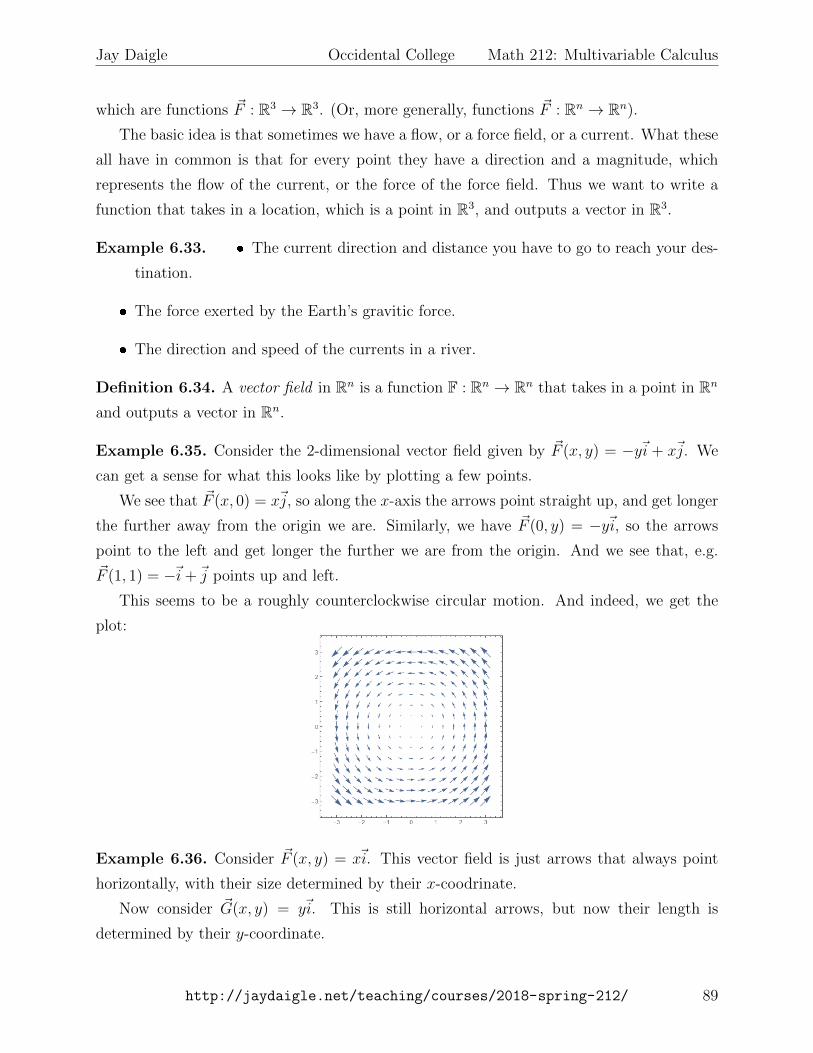
Example 6.35. Consider the 2-dimensional vector field given by ~F (x, y) = −y~i + x~j. We

can get a sense for what this looks like by plotting a few points.

We see that ~F (x, 0) = x~j, so along the x-axis the arrows point straight up, and get longer

the further away from the origin we are. Similarly, we have ~F (0, y) = −y~i, so the arrows

point to the left and get longer the further we are from the origin. And we see that, e.g.

~F (1, 1) = −~i+~j points up and left.

This seems to be a roughly counterclockwise circular motion. And indeed, we get the

plot:

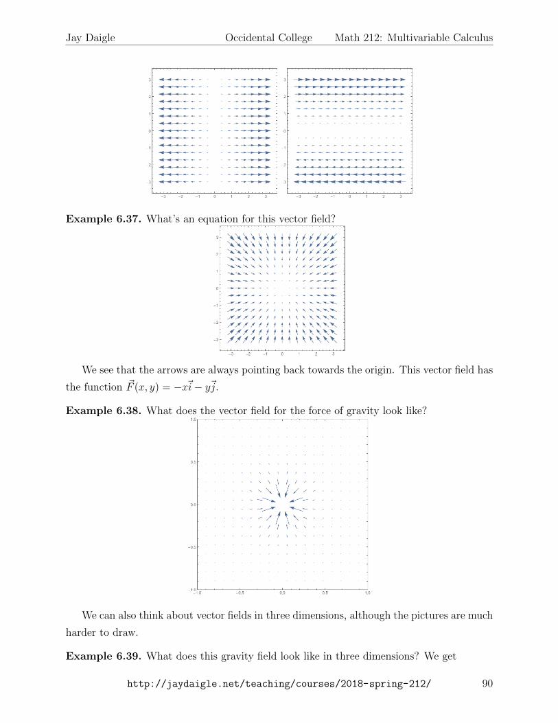
Example 6.36. Consider ~F (x, y) = x~i. This vector field is just arrows that always point

horizontally, with their size determined by their x-coodrinate.

Now consider ~G(x, y) = y~i. This is still horizontal arrows, but now their length is

determined by their y-coordinate.




Example 6.37. What’s an equation for this vector field?

We see that the arrows are always pointing back towards the origin. This vector field has

the function ~F (x, y) = −x~i− y~j.

Example 6.38. What does the vector field for the force of gravity look like?

We can also think about vector fields in three dimensions, although the pictures are much

harder to draw.

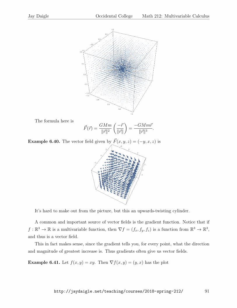
Example 6.39. What does this gravity field look like in three dimensions? We get




The formula here is

~F (~r) =GMm

‖~r‖2

(−~r‖~r‖

)=−GMm~r

‖~r‖3.

Example 6.40. The vector field given by ~F (x, y, z) = (−y, x, z) is

It’s hard to make out from the picture, but this an upwards-twisting cylinder.

A common and important source of vector fields is the gradient function. Notice that if

f : R3 → R is a multivariable function, then ∇f = (fx, fy, fz) is a function from R3 → R3,

and thus is a vector field.

This in fact makes sense, since the gradient tells you, for every point, what the direction

and magnitude of greatest increase is. Thus gradients often give us vector fields.

Example 6.41. Let f(x, y) = xy. Then ∇f(x, y) = (y, x) has the plot




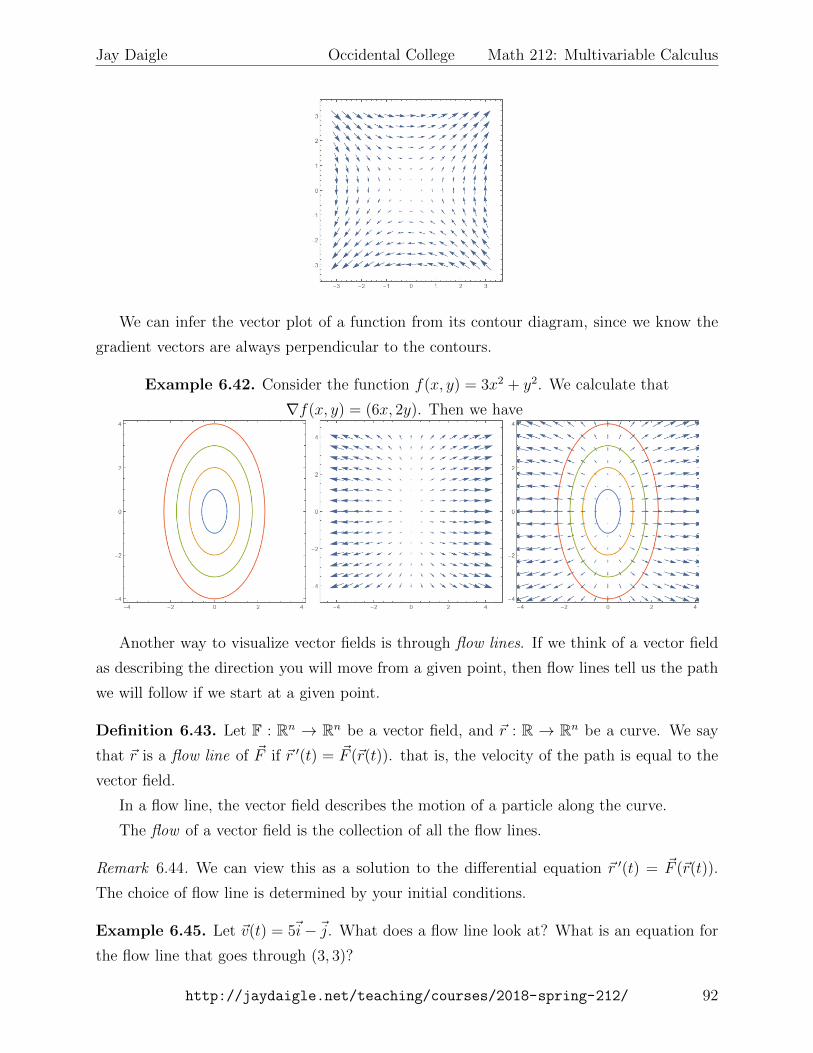
We can infer the vector plot of a function from its contour diagram, since we know the

gradient vectors are always perpendicular to the contours.

Example 6.42. Consider the function f(x, y) = 3x2 + y2. We calculate that

∇f(x, y) = (6x, 2y). Then we have

Another way to visualize vector fields is through flow lines. If we think of a vector field

as describing the direction you will move from a given point, then flow lines tell us the path

we will follow if we start at a given point.

Definition 6.43. Let F : Rn → Rn be a vector field, and ~r : R → Rn be a curve. We say

that ~r is a flow line of ~F if ~r ′(t) = ~F (~r(t)). that is, the velocity of the path is equal to the

vector field.

In a flow line, the vector field describes the motion of a particle along the curve.

The flow of a vector field is the collection of all the flow lines.

Remark 6.44. We can view this as a solution to the differential equation ~r ′(t) = ~F (~r(t)).

The choice of flow line is determined by your initial conditions.

Example 6.45. Let ~v(t) = 5~i−~j. What does a flow line look at? What is an equation for

the flow line that goes through (3, 3)?




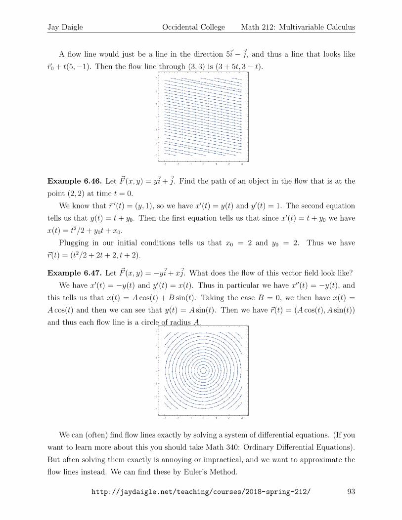
A flow line would just be a line in the direction 5~i − ~j, and thus a line that looks like

~r0 + t(5,−1). Then the flow line through (3, 3) is (3 + 5t, 3− t).

Example 6.46. Let ~F (x, y) = y~i +~j. Find the path of an object in the flow that is at the

point (2, 2) at time t = 0.

We know that ~r ′(t) = (y, 1), so we have x′(t) = y(t) and y′(t) = 1. The second equation

tells us that y(t) = t+ y0. Then the first equation tells us that since x′(t) = t+ y0 we have

x(t) = t2/2 + y0t+ x0.

Plugging in our initial conditions tells us that x0 = 2 and y0 = 2. Thus we have

~r(t) = (t2/2 + 2t+ 2, t+ 2).

Example 6.47. Let ~F (x, y) = −y~i+ x~j. What does the flow of this vector field look like?

We have x′(t) = −y(t) and y′(t) = x(t). Thus in particular we have x′′(t) = −y(t), and

this tells us that x(t) = A cos(t) + B sin(t). Taking the case B = 0, we then have x(t) =

A cos(t) and then we can see that y(t) = A sin(t). Then we have ~r(t) = (A cos(t), A sin(t))

and thus each flow line is a circle of radius A.

We can (often) find flow lines exactly by solving a system of differential equations. (If you

want to learn more about this you should take Math 340: Ordinary Differential Equations).

But often solving them exactly is annoying or impractical, and we want to approximate the

flow lines instead. We can find these by Euler’s Method.




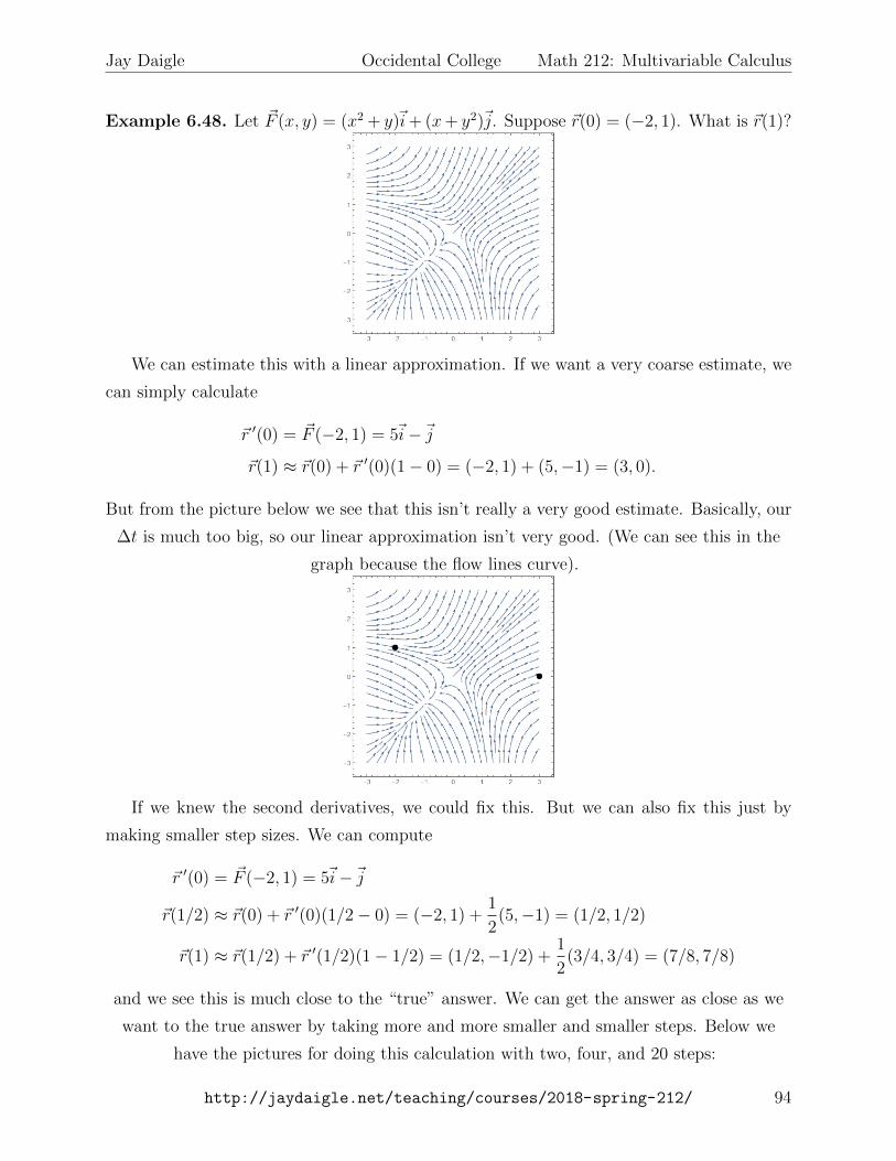
Example 6.48. Let ~F (x, y) = (x2 + y)~i+ (x+ y2)~j. Suppose ~r(0) = (−2, 1). What is ~r(1)?

We can estimate this with a linear approximation. If we want a very coarse estimate, we

can simply calculate

~r ′(0) = ~F (−2, 1) = 5~i−~j

~r(1) ≈ ~r(0) + ~r ′(0)(1− 0) = (−2, 1) + (5,−1) = (3, 0).

But from the picture below we see that this isn’t really a very good estimate. Basically, our

∆t is much too big, so our linear approximation isn’t very good. (We can see this in the

graph because the flow lines curve).

If we knew the second derivatives, we could fix this. But we can also fix this just by

making smaller step sizes. We can compute

~r ′(0) = ~F (−2, 1) = 5~i−~j

~r(1/2) ≈ ~r(0) + ~r ′(0)(1/2− 0) = (−2, 1) +1

2(5,−1) = (1/2, 1/2)

~r(1) ≈ ~r(1/2) + ~r ′(1/2)(1− 1/2) = (1/2,−1/2) +1

2(3/4, 3/4) = (7/8, 7/8)

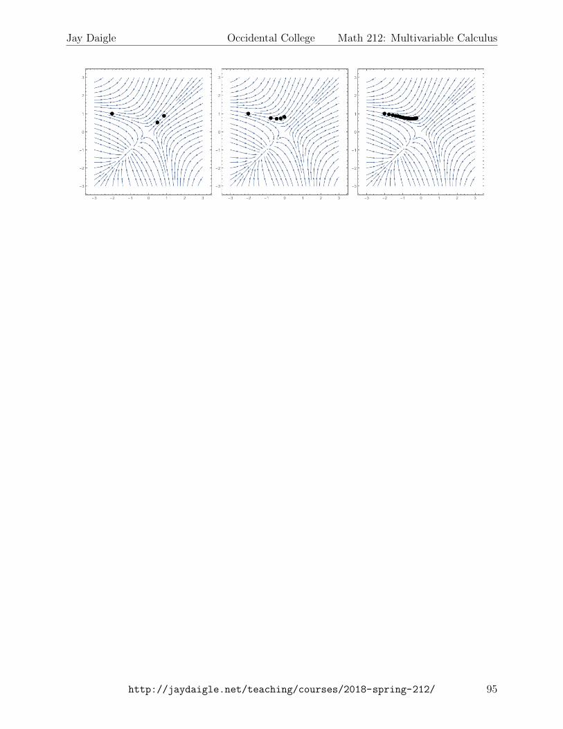
and we see this is much close to the “true” answer. We can get the answer as close as we

want to the true answer by taking more and more smaller and smaller steps. Below we

have the pictures for doing this calculation with two, four, and 20 steps:






6 Parametrization and Vector Fields - Jay Daigle

Documents