6 MATHEMATICAL MODELS IN MECHANICSuser.engineering.uiowa.edu/~kkchoi/Chapter_6.pdf6 MATHEMATICAL MODELS IN MECHANICS ... Theorem 6.1.2 (Green's Theorem). If real valued functions P(x1,

6

MATHEMATICAL MODELS IN MECHANICS

As an introduction to the study of partial differential equations that arise in engineering applications, it is helpful to define a set of model problems that contain many of the features of more complex applications. The differential equations that govern these model problems are derived, using techniques that may be employed in more general applications. The resulting equations represent typical models of more general field equations that are encountered in fluid dynamics, elasticity, and heat transfer. The purpose of this chapter is to illustrate methods of obtaining the governing equations for such problems. The differential equations derived here are studied in Chapters 7 and 8, where methods for solving specific classes of equations are developed and applied.

6.1 MULTIPLE INTEGRAL THEOREMS

Since the study of mechanics often deals with static and dynamic behavior of material or energy that is continuously distributed over one or more space dimensions, a method is required to quantify the properties of the material state, such as mass, momentum, volume, and other quantities that are associated with an infinite number of points that make up the continuum. Such quantities can be described in terms of multiple integrals. A few multiple integral theorems play a critical role in quantitatively expressing physicallaws that govern the state of a continuum. It is presumed that the reader is familiar with definitions and basic ideas of integration. The purpose of this section is to summarize multiple integral properties and theorems and derive results that will be used in the study of techniques for modelling the behavior of continua. A minimal number of proofs are included in this section. The interested reader is referred to Refs. 8 and 9 for details.

Properties of Multiple Integrals

Consider an area A in R2 and a volume Yin R3, both of which represent physical domains that are bounded by smooth curves and surfaces, respectively. A function f(x) denotes a scalar valued function of the vector variable x in either R 2 or R3. The integral of such scalar valued functions over an area A or volume Y is denoted as

J JA f(x) dx1 dx2, J J J v f(x) dx1 dx2 dx3 (6.1.1)

230

Sec. 6.1 MuHiple Integral Theorems 231

If c is a scalar and g(x) is a second function, then the following linear properties of multiple integrals hold:

J JA c f(x) dx1 dx2 = c J JA f(x) dx1 dx2

J J fv c f(x) dx1 dx2 dx3 = c J J fv f(x) dx1 dx2 dx3

J J A [ f(x) + g(x) ] dx 1 dx2 = J J A f(x) dx 1 dx2

+ J J A g(x) dxl dx2

J J Jv [ f(x) + g(x)] dx1 dx2 = J J Jv f(x) dx1 dx2 dx3

+ J J Jv g(x) dx1 dx2 dx3

(6.1.2)

If an area A is subdivided into areas A1 and A2, as shown in Fig. 6.1.1, and a volume V is likewise subdivided into volumes V 1 and V 2, then

(6.1.3)

Figure 6.1.1 Subdivision of Area A

If f(x) S g(x) throughout an area A or volume V, then

232 Chap. 6 Mathematical Models in Mechanics

(6.1.4)

It follows that, since - I f(x) I ~ f(x) ~ I f(x) I, Eq. 6.1.4 may be applied to obtain

I f fA f(x) dx1 dxzl ~ J fA I f(x) I dx1 dx2

I f f fv f(x) dx1 dxz dx31 S f f fv I f(x) I dx1 dx2 dx3

(6.1.5)

The Mean Value Theorem and Leibniz's Rule

An important result for derivation of differential equations of continuum mechanics is the Mean Value Theorem, which holds for a simply connected region; i.e., a region for which each closed curve or surface in the region encloses only points in the region. There are, thus, no holes in simply connected regions.

Theorem 6.1.1 (Mean Value Theorem). If the function f(x) is continuous in a simply connected area A or volume V, then there is a point x in A or V such that

f J fv f(x) dx1 dx2 dx3 = V f(i)

i.e., the function f(x) achieves its mean value at x.

Example 6.1.1

(6.1.6)

• The average value of f(x1, x2) = ax1- x12 on the rectangle -a~ x1 ~a, 0 ~ x2 ~ 1, can be found from

A = a - (-a) = 2a

and Eq. 6.1.6 may be used to obtain the mean value f(x) = -(2/3) ( a3/2a) = -a2/3, which gives x 1 = ( 1 - ...J 7/3 ) ( a/2) and x2 is any value in (0, 1 ). •

Sec. 6.1 MuHiple Integral Theorems 233

While Eq. 6.1.6 is not particularly useful from a computational point of view, it is often important to know that there is a point in a region of a continuum such that the integral can be expressed as the value of the integrand at that point times the area or volume of the region.

To illustrate use of the Mean Value Theorem, and as a precursor to development of derivative formulas associated with integrals, consider the integral of a function over an interval, where both the function and the end points depend on a scalar parameter a,

Jb(a)

J(a) = f(x, a) dx a( a)

(6.1.7)

It is clear that the value of this integral is a function of the parameter a, as indicated by the notation J(a). To differentiate this expression with respect to a, form the difference quotient

J( a+ 0)- J(a) 1 { J b(a+l)) J b(a) } 0 = B f(x, a+o) dx - f(x, a) dx

a(a+l)) a(a)

1 { J b(a+l)) J a(a+l)) = B f(x, a+o) dx- f(x, a+o) dx

b(a) a(a)

J b(~ } + [ f( x, a+ o ) - f(x, a) ] dx a( a)

If all functions involved are continuous, the Mean Value Theorem may be applied to each integral, to obtain

J(a+oi- J(a) = [ b(a+o~- b(a) J f(X., a+o)

_ [ a(a+o~- a(a) J f(~. a+o)

+ J b(a) [ f( x, a+ o ) - f(x, a) J dx a(a) 0

where xis between b(a) and b( a+ 0) and x is between a( a) and a( a+ o ). Assume now that the functions a( a), b(a), and f(x, a) are differentiable with respect to a. Taking the limit of both sides of the above expressions as o approaches 0, Leibniz's Rule of Differentiation is obtained as

dJ db da J b(a) af(x a) -d = -d f(b(a), a) - -d f(a(a), a) + a' dx

a a a a(a) a (6.1.8)


Example 6.1.2

Consider the following integral, which depends on a.:

Using Leibniz's Rule of Differentiation, the derivative ofF( a) is

a3

F'(a.) = 3a.2 tan ( a7 ) - 2a. tan ( a.5 ) + J a 2 x2 sec2 ( a.x2 ) dx •

Line and Surface Integrals

If Cis a continuous curve in R2 and Sis a connected surface in R3, then line integrals and surface integrals of a function f(x) on R2 and R3, defined on C and S, respectively, are denoted as

fc f(x) dC, (6.1.9)

where dC and dS are differential arc length and differential surface area on the curve C and the surfaceS, respectively. These integrals obey the same linearity, inequality, and mean value properties of Eqs. 6.1.2- 6.1.6. Such line and surface integrals play a key role in describing motion of material and energy across curves or surfaces in a continuum and are used frequently in developing governing equations for continuum behavior.

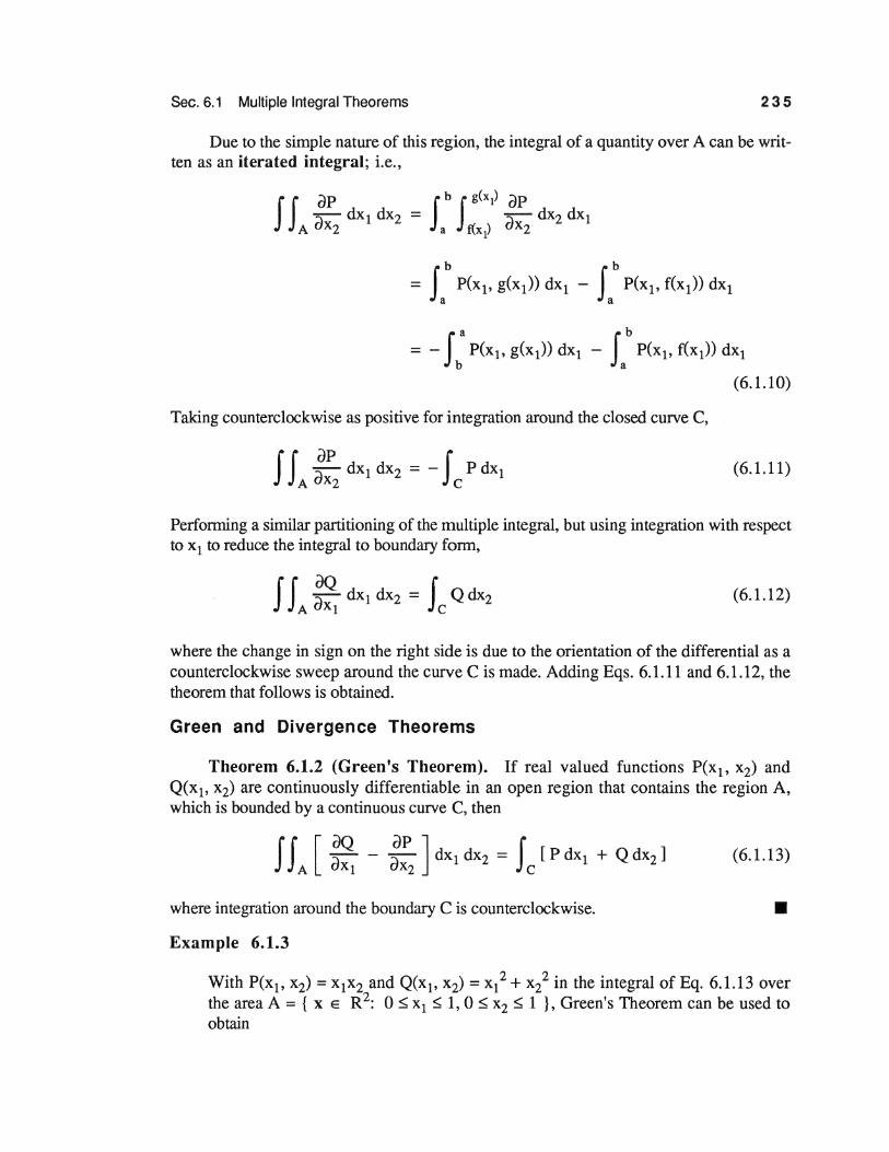
Let P(x) and Q(x) be scalar valued functions defined in R2• It is assumed that these functions are continuously differentiable on an open set in R2 that contains a region A that is bounded by a closed curve C, as shown in Fig. 6.1.2. Note that the region A has been selected so that a vertical line intersects curve C in only two points. A more complex region may be subdivided into several regions that satisfy such a condition.

n

a b

Figure 6.1.2 Domain of Integration

Sec. 6.1 Multiple Integral Theorems 235

Due to the simple nature of this region, the integral of a quantity over A can be written as an iterated integral; i.e.,

= - J: P(xl, g(x1)) dx1 - Jab P(x1, f(x1)) dx1

(6.1.10)

Taking counterclockwise as positive for integration around the closed curve C,

(6.1.11)

Performing a similar partitioning of the multiple integral, but using integration with respect to x1 to reduce the integral to boundary form,

(6.1.12)

where the change in sign on the right side is due to the orientation of the differential as a counterclockwise sweep around the curve Cis made. Adding Eqs. 6.1.11 and 6.1.12, the theorem that follows is obtained.

Green and Divergence Theorems

Theorem 6.1.2 (Green's Theorem). If real valued functions P(x1, x2) and Q(x1, x2) are continuously differentiable in an open region that contains the region A, which is bounded by a continuous curve C, then

(6.1.13)

where integration around the boundary C is counterclockwise. • Example 6.1.3

With P(x1, x2) = x1x2 and Q(x1, x2) = x12 + xl in the integral of Eq. 6.1.13 over the area A = { x e R2: 0 s;; x1 s;; 1, 0 S x2 S 1 }, Green's Theorem can be used to obtain


- .!. x211 - .!. - 2 1 - 2 0 •

From the diagram of Fig. 6.1.3, the unit normal and unit tangent vectors n and s, respectively, may be written as

(6.1.14)

where n1 and n2 are the direction cosines of the normal n. A vector valued function F(x) = [ F1 (x), F2(x) ]T may be integrated over the boundary C, in terms of either differential coordinates or differential arc length, as

L FTs dC = L [ F1, F2 ] [ ~:2] dC

= J c ( - F1 cos f3 + F2 cos a ) dC

n

A -1 n ..., =cos n2 = a+ 2

~----------------------------------------~ x1

Figure 6.1.3 Differential Arc dC

(6.1.15)


The geometric relations of Fig. 6.1.3 and Green's Theorem can be used to obtain

fcFTndC = fc[F1n1 + F2n2 ]dC = fc[F1 dx2 - F2 dxtJ

(6.1.16)

Defining the gradient operator as V = [ a:l, a:2 ]T in R2 and

v = [ :~.a , :~.a , :~.a JT in R3, VTF(x) = div F(x) is called the divergence of a ux1 ux2 ux3

vector valued function F(x), and the following theorem is obtained.

Theorem 6.1.3 (Divergence Theorem). If the vector valued function F(x) = [ F1 (x), F2(x) ]T is continuously differentiable in an open region of R2 that contains the domain A, which is bounded by the smooth curve C, then

J JA divFdx1dx2 = J JA VTFdx1dx2 = fcFTndC (6.1.17)

In a three dimensional space, an analogous formula holds; i.e.,

(6.1.18)

where F(x) = [ F1 (x), F2(x), F3(x) ]T is a continuously differentiable vector valued function in an open region ofR3 that contains V, which is bounded by a smooth surfaceS, and n(x) is the unit outward normal to surface S. •

For proof of the three dimensional Divergence Theorem, the reader is referred to Ref. 8.

Example 6.1.4

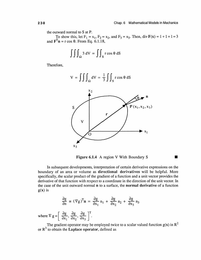
LetS be the surface of a region V of R3, as shown in Fig. 6.1.4, for which the Divergence Theorem is applicable. Let 0 be the origin of the coordinate system and let P(x1, x2, x3) be ii variable point on S. Then, the volume of the region is

Vol = J J J s r cos e dS

where r = I r I is the distance OP and e is the angle between the directed line OP and


the outward normal to S at P. To show this, let F1 = x1, F2 = x2, and F3 = x3• Then, div F(x) = 1 + 1 + 1 = 3

and FTn = r cos 9. From Eq. 6.1.18,

Therefore,

v = J J J 0 dV = ~ J J s r cos e dS

Figure 6.1.4 A region V With Boundary S • In subsequent developmeFlts, interpretation of certain derivative expressions on the

boundary of an area or volume as directional derivatives will be helpful. More specifically, the scalar product of the gradient of a function and a unit vector provides the derivative of that function with respect to a coordinate in the direction of the unit vector. In the case of the unit outward normal n to a surface, the normal derivative of a function g(x) is

[ ()g ()g ()g JT whereVg= ~. ~. :r- . ux1 ux2 ux3

The gradient operator may be employed twice to a scalar valued function g(x) in R2

or R3 to obtain the Laplace operator, defined as


(6.1.19)

Employing Eqs. 6.1.17 and 6.1.18, with F = Vg and Eq. 6.1.19, Green's Identities are obtained as

J J A V2g dx1 dx2 = Jc (Vg)Tn dC = Jc ~! dC (6.1.20)

J J Jv V2g dx1 dx2 dx3 = J Js (Vg)Tn dS = J Js * dS

for R2 and R3, respectively. From Eq. 6.1.16, with Fi = uv and Fj = 0, i :1: j, the following identity is obtained:

Jc uvni dC = J JA a~:~) dx1 dx2

= J J AU :i dx1 dx2 + J J A V ~:i dx1 dx2

This important result is summarized in the form of a theorem.

Theorem 6.1.4 (Integration by Parts). Let u(x) and v(x) be in C1(A), where A is a region in R2 with a smooth boundary C. Then,

J J A u ~:i dx 1 dx2 = J c uvni dC - J J A v ~:i dx 1 dx2 (6.1.21)

Similarly, if u(x) and v(x) are in C1(V), where V is a region in R3 with a smooth boundary, then

J J J v u ~;i dx 1 dx2 dx3 = J J s uvni dS - J J J v v ~:i dx 1 dx2 dx3

(6.1.22)

• Note the similarity between Eqs. 6.1.21 and 6.1.22 and the elementary integration

by parts formula [8, 9],

Jb du lb Jb dv

a v dx dx = v(x) u(x) a - a u dx dx


The Implicit Function Theorem

A final topic that is important in studying continuum behavior is the transformation of an integral quantity associated with the continuum. First, recall the standard implicit function theorem from advanced calculus [8].

Theorem 6.1.5 (Implicit Function Theorem). Let Yi• i = 1, ... , n, denote a set of coordinates in Rn, with the usual Cartesian system denoted xi, i = 1, ... , n. Let the coordinate systems be related by the transformation

xi = gi(y), i = 1, ... , n (6.1.23)

where the functions gi(Y) are differentiable. Equation 6.1.23 can be solved for y as a differentiable function of x in a neighborhood of each pointy in Rn if the Jacobian matrix of the functions gi(y) is nonsingular; i.e.,

Example 6.1.5

Consider the coordinate transformation

Since

X1 = gl(y) = Y1 + 2y2

x2 = g2(Y) = 3yl + Y2

I [ a~~;) J I = I! ~ I = - 5 # o

(6.1.24)

•

by the Implicit Function Theorem, the above equation can be solved to obtain

Example 6.1.6

Y1 = f1(x) = (- x1 + 2x2) I 5

Y2 = f2(x) = ( 3x1 - x2)/5 • Consider the transformation between x-y Cartesian coordinates and r-8 polar coordinates, given as

X = gl(r, 8) = rCOS 8

y = g2(r, 8) = r sin 8

The determinant of the Jacobian matrix of this transformation is


agl agl ar ae

ag2 ag2 ar ae

= I [ c~s 88 - r sineS] I = r cos2 8 + r sin2 8 = r sm rcos

As long as r ::t 0, by the Implicit Function Theorem, this coordinate transformation can be solved to yield

r = ,Jx2 + y2

8 -1 y =tan -X •

Often, variables will be changed to describe an area or volume in R 2 or R 3, over which a multiple integral is to be evaluated. Denote by A' and V' the transformed area and volume A and V, respectively, where the equations of transformation are as in Eq. 6.1.23.

Theorem 6.1.6. If the transformation of coordinates of Eq. 6.1.23 is continuously differentiable and if Eq. 6.1.24 holds, then for domains A and V in R2 and R3, respectively, with smooth boundaries,

J J A F(x) dx1 dx2 = J L F(g(y)) I [ il~~;> ] I dy1 dy2

(6.1.25)

• For proof, the reader is referred to Ref. 8.

EXERCISES 6.1

1. Show that if two functions f(x) and g(x) are continuous and if

or

J J J v f dx1 dx2 dx3 = J J J v g dx1 dx2 dx3

for all regions A and V in R2 or R3, respectively, then f(x) = g(x) throughout R2 and R3, respectively.


Ja . dUe> 2. Let J(e) = 0 sm (X+ e) dx. Compute de by

(a) using Leibniz's rule.

(b) evaluating the defmite integral and then differentiating with respect to e. 3. Let u(x) and v(x) be scalar valued functions in C2(A), where A is a domain in R2

with a continuous boundary C.

(a) Show that VT(uVv) = (Vu)T(Vv) + uV~; i.e.,

a: 1 ( u ;;1 ) + a:2 ( u ;;2 ) = [ ;;1 · ;;2 J[ £~] dX2

[ a2v rPv] +u -+-

axr ax~

(b) Apply the Divergence Theorem to prove Green's Formulas

and

J c [ u ~: - v ~~ J dC = J J A [ u V~ - v V2u ] dx1 dx2

4. Show that the results of Exercise 3 hold in R3, with C replaced by Sand A replaced byV.

5. Let u(x) and v(x) be in C2(A), with u(x) = v(x) = 0 on the boundary C of A. Show that, in this case,

J J A v V2u dx1 dx2 = J J Au V2v dx1 dx2 6. Show that if u(x) is in C2(A) and u(x) = 0 on the boundary C of A, then

-J J Au V2u dx1 dx2 ~ 0

7. Extend Exercise 6 to R 3.

8. Let p(x) denote the pressure in a three dimensional flow field. Let p(x) be differentiable and let V be a volume element of fluid with boundary S. Use the Divergence Theorem to transform the net force on S due to pressure pin the xi direction; i.e.,

-J fs pni dS, to an integral overV, namely,- J J Jv ~~i dx1 dx2 dx3.

Sec. 6.2 Material Derivative and Differential Forms 243

6.2 MATERIAL DERIVATIVE AND DIFFERENTIAL FORMS

Certain key concepts that are not apparently associated with multiple integral theorems play an important role in development of the governing equations of continuum behavior. Specifically, material derivatives are important in deriving the differential equations of motion for a continuum. The theory of differential forms also plays a key role in conservation laws of mechanics, as a direct result of multiple integral theorems.

Description of a Continuum

In this section, a continuum will be considered as a region of space that is composed of an infinite number of material particles. To keep track of these particles, a coordinate system is chosen and the coordinates of a particle at timet= 0 are a= [at' a2, a3 ]T. At a later time, the particle has moved to physical coordinates x = [ x1, x2, x3 ] . Thus, motion of the particles is described by the equations

(6.2.1)

where a locates the particle at t = 0. It is presumed that the functions xi(a, t) are continuously differentiable and that the determinant of the Jacobian matrix of their derivatives with respect to the ai does not vanish. Thus, a can be determined as a function of x and t. Consider a volume V that is made up of a collection of material particles at time t = 0. As time progresses, this volume will deform as the particles move. The deformed volume at timet is denoted V(t).

Example 6.2.1

A basic quantity in the study of motion is the mass of a collection of material points, which must be preserved. Thus, the law of conservation of mass may be written, in terms of material density p0(a) at timet= 0 and p(x(a, t)) at timet, as

J J J p(x(a, t)) dx1 dx2 dx3 = J J J p0(a) da1 daz da3 V(t) V(O)

(6.2.2)

where the integral on the left is taken over the deformed volume at time t and the integral on the right is taken over the initial volume of material at time t = 0. Employing Eq. 6.1.25, variables in the integral on the left side of Eq. 6.2.2 can be changed, to obtain

J J J V(O) p(x(a, t)) I [ ::; ] I da1 da, da3

= J J J p0(a) da1 da2 da3 V(O)

(6.2.3)

Since Eq. 6.2.3 must hold for any volume element in the continuum, V(O) can be taken as a very small neighborhood of point a. The Mean Value Theorem, as ex-


pressed by the second of Eqs. 6.1.6, yields

Vol(O)[ p(x(ii, t)) [ ::J -p0(a)] = 0

for some point a in V(O), where Vol(O) is the volume ofV(O). Since Vol(O) * 0,

[ dx·] p(x(a, t)) --!. - p0(a) = o da· J

Letting V(O) shrink to the point a, since all terms appearing are continuous in a and a must converge to a,

p(x(a, t)) --!. [ dX·] da· J

= Po(a) (6.2.4)

This provides a relationship between the initial density p0(a) and the density p(x(a, t)) at any time during the continuum motion. •

There are many integral quantities in continuum behavior that vary with time. Typi-cally, consider the integral

J(t) = J J J f(x, t) dx 1 dx2 dx3 V(t)

(6.2.5)

where f(x, t) denotes a property of the continuum, such as the density in Eq. 6.2.2. It is important to be able to detennine the rate of change of the quantity J with time, for the set of particles that occupy V(t). Any given particle at timet is located at a point x. After a differential time ~t, it will move to the new position x' = x + v~t, where vis its velocity. At timet+ ~t, the boundary S of V will deform to a neighboring surface S', which bounds the deformed volume V' = V(t + ~t) of Fig. 6.2.1.

dV= vi ni~tdS

Figure 6.2.1 Deformation of a Moving Volume


Material Derivative

Define the material derivative of J(t) in Eq. 6.2.5 as

(6.2.6)

There are two integral contributions to the difference on the right side of Eq. 6.2.6; one over the common domain V0 of V and V' and the other over the region V 1, where V and V' differ. The former contribution to the limit in Eq. 6.2.6 is simply

. J J J [ f(x', t + ~t) - f(x, t) J lim A dx1 dx2 dx3 6t~O y 0 t

- JJJ af(x, t) dx d d - :'1 1 x2 x3

y ut (6.2.7)

since in the limit as At approaches 0, V0 approaches V. The contribution due to motion normal to surface S is determined by the normal dis

placement of particles on the boundary S, which is viniAt, where ni are direction cosines of the outer normal n of S and summation notation is used. The volume within V 1 that is swept out by particles that occupy an element of area AS on S is A V = viniAtAS. Thus, the contribution to the integral of Eq. 6.2.6 from V 1 is

lim ! J J J f(x', t +At) vini At ds = J J f(x, t) vini ds 6t~O ut y 1 S(t)

Adding this to the contribution over V0 from Eq. 6.2.7, the material derivative of J(t) is

ddJ = dd J J J f(x, t) dx1 dx2 dx3 t t V(t)

J J J a f(x, t) J J = a dx1 dx2 dx3 + f(x, t) vini dS vw t sw (6.2.8)

It is interesting to note that this result is an extension of Leibniz's rule of differentiation of Eq. 6.1.8.

The surface integral in Eq. 6.2.8 is precisely the right side of Eq. 6.1.18, if the vector F is interpreted as having components Fi = fvi. Equation 6.1.18 then yields (note that summation notation is used)


~: = J J J v<t> [ ~: + a:i ( fvi ) J dx1 dx2 dx3 (6.2.9)

a af dx· av. Noting that -a ( fvi ) = -a -d 1 + f -0 1

, Eq. 6.2.9 can be rewritten as xi xi t xi

ddJ = dd J J J f(x, t) dxl dx2 dx3 t t V(t)

= JJJ [ df(x, t) + f avi(x, t)] dx dx dx V(t) dt axi 1 2 3

(6.2.10)

which is a useful alternate form of the material derivative of J(t). Equations 6.2.8 and 6.2.10 are alternate forms of the material derivative of the

spatial integral of the function f(x, t) over the volume V(t), which is moving with time. They play an important role in deriving the equations of fluid mechanics and other applications in which movement of the continuum occurs over time.

Example 6.2.2

Continuing with Example 6.2.1 involving the total mass in a given volume, as in Eq. 6.2.2, note that if mass is neither created nor destroyed in a given flow field, then for a fixed set of particles that occupy a continuously deforming volume V(t),

;t JJJ p(x, t) dx1 dx2 dx3 = 0 V(t)

(6.2.11)

Employing Eq. 6.2.10, this results in the integral form of the law of conservation of mass

JJJ [ dp(x, t)

V(t) dt (6.2.12)

or, using Eq. 6.2.8,

JJJ ap(x, t) JJ a dx1 dx2 dx3 + p(x, t) vi(x, t) ni dS = 0 V(t) t S(t)

(6.2.13)

If the integrand in Eq. 6.2.12 is continuous, then by the Mean Value Theorem, there is a point i in V(t) where

dp(i,t) - avi(i,t) dt + p(x, t) ax. = 0

1


Since the volume element V(t) is arbitrary, it can be shrunk to any point to yield the differential equation form of the law of conservation of mass (often called the continuity equations) as

or

dp avi -+p-a =O dt xi

a ( pvi) a = o X· 1

(6.2.14)

These continuity equations will be used in a later section to study fluid flow. Note that Eq. 6.2.14 is valid only if p and vi have continuous flrst derivatives. Even if these functions are not differentiable, Eq. 6.2.12 or Eq. 6.2.13 still have physical significance, as laws of conservation of mass. •

Differential Forms

A differential expression

fi(x) dxi (6.2.15)

where summation notation is used, is called a differential form in n variables. Such differential forms arise often in the study of problems of mechanics.

Example 6.2.3

For x e R3, the following expressions are differential forms:

fi(x) dxi = 2x2x3 dx1 + x1x3 dx2 + x1x2 dx3

gi(x) dxi = 2x1x2x3 dx1 + x12x3 dx2 + x12x2 dx3

Note that the second differential form is simply the product of x1 and the first differential form. •

Definition 6.2.1. The differential form of Eq. 6.2.15 is said to be an exact differential form at point x if there is a differentiable function F(x), defined in a neighborhood of x, such that

dF(x) = fi(x) dxi (6.2.16)

at all points in this neighborhood; i.e., if fi(x) = a :(x). xi •

Theorem 6.2.1. Let D be a simply connected open region in Rn and let fi(x) have continuous flrst partial derivatives in D. Then, the differential form of Eq. 6.2.15 is exact in D if and only if


i, j = 1, ... , n (6.2.17)

at each point in D. Further, if the form is exact in D, the function F(x) in Eq. 6.2.16 may be written as a line integral

F(x) - F(a) = J c fi(x) dxi (6.2.18)

where Cis any smooth curve in the domain D from point a to point x. Finally, the integral in Eq. 6.2.18 is independent of the path C. •

This theorem is proved here for n = 2. The proof for n ~ 3, the interested reader is referred to Refs. 3 and 8.

To show that the conditions of Eq. 6.2.17 are necessary, it will be shown that Eq. 6.2.17 holds when the function F(x) satisfies

f( ) _ oF(x) . X - ':1 1 oX· 1

(6.2.19)

Since the functions fi(x) are continuously differentiable, the function F(x) is twice continuously differentiable. Differentiating both sides of Eq. 6.2.19 with respect to xj yields

() fi(x) ()2F(x) o2F(x) ()fix) OX· = OX· OX· = ax. OX· = OX· (6.2.20)

J J 1 1 J 1

which is Eq. 6.2.17, as was to be shown. Conversely, beginning with the assumption that Eq. 6.2.17 holds, it must now be

shown that a function F(x) satisfying Eq. 6.2.16 exists and is given by Eq. 6.2.18. Choosing any fixed point a in D, let x1 be any other point in D. Let C be a smooth curve from a to x1 and define

(6.2.21)

Let C1 be any other smooth path to x1 in the domain D, as shown in Fig. 6.2.2.

a

Figure 6.2.2 Paths From a to x 1


It will now be shown that

(6.2.22)

which will show that the integral ofEq. 6.2.18 is independent of path from a to x1• This is equivalent to showing that the line integral of fi(x) dxi, around the closed curve in Fig. 6.2.2, is zero. Denoting this curve as r and the interior of the curve as region A, Green's Theorem (Theorem 6.2.1) can be used to obtain

(6.2.23)

where the integral over A is zero, by virtue of Eq. 6.2.17. Thus, the integral identity of Eq. 6.2.22 holds. This completes the proof of the theorem for n = 2. •

Example 6.2.4

To see if the differential forms of Example 6.2. 3 are exact, note that

so the ftrst differential form is not exact. Thus, there is no function F(x) for which dF(x) = fi(x) dxi.

For the second differential form,

a gl (x) = 2x1x3 =

a g2(x)

ax2 axl

a gl(x) = 2XtX2 =

a g3(x)

ax3 axl

a g2(x) xi

a g3(x)

ax3 = = ax2

so the second differential form is exact. In fact, a simple calculation shows that for G(x) = x12x2x3, d G(x) = gi(x) dxi. The factor u(x) = x1 that multiplies the ftrst differential form, which is not exact, to obtain the second differential form, which is exact, is called an integrating factor. •

As an application of the theory of exact differential forms in mechanics, consider the work done on an n-dimensional mechanical system, with generalized coordinates x and generalized force f(x) in Rn. The work done on the system in undergoing a differential displacement dx is


(6.2.24)

The total work done in displacing the system from point x1 to point x2, over a curve C, may be written as the integral

(6.2.25)

According to Theorem 6.2.1, this work is independent of the path C from x1 to x2, if and only if the differential form fi(x) dxi is exact; i.e., if and only if Eq. 6.2.17 holds. Mechanical systems for which work done by a force field is independent of path traversed are called conservative systems.

EXERCISES 6.2

1. Let V be a volume element in a flow field, with boundaries as in Exercise 8 of Section 6.1. Compute the time derivative of the momentum in the xi direction; i.e.,

dd J J J p(x, t) vi(x, t) dx1 dx2 dx3 t V(t)

2. Determine whether the following differential forms are exact:

3. If the factor u(x) = x1 is multiplied through the differential form of Exercise 2 (b) above, show that u(x) gi(x) dxi is exact.

4. Find functions F(x) and G(x) such that, for the differential forms fi(x) dxi and u(x) gi(x) dxi of Exercises 2 and 3,

aF(x) dF(x) = a dx· = f-(x) dx· X· 1 1 1

1

ao(x) dG(x) = a dxi = u(x) gi(x) dxi

X· 1

5. Evaluate the integral

f ( 2 x 2 dx + 2 y 2 dy ) s x-y y-x

where Sis a curve from (1, 0) to (5, 4) and lies between the lines y = x andy= -x.

Sec. 6.3 Vibrating Strings and Membranes 251

6.3 VIBRATING STRINGS AND MEMBRANES

The simplest examples of continuum mechanics problems that contain the basic elements found in more complex applications are strings and membranes [11, 17, 18]. These bodies represent the effect of distributed mass over one and two space dimensions, while avoiding the technical complexity of distributed systems that require higher order differential operators to represent force-displacement relations.

The Transversely Vibrating String

A string is fixed at both ends, as shown in Fig. 6.3.1(a). The abscissa x in this graph is a physical coordinate that is measured along the undeformed string and the ordinate u represents displacement of the string. For a given set of initial conditions (position and velocity) and applied forces, the string will move, or vibrate, in the plane of the applied loads. Denoting the time coordinate by t, the displacement function of the string will be a function of both the space and time variables; i.e., u = u(x, t).

u

(a) deflected string (b) free body diagram

Figure 6.3.1 Vibrating String

The string is initially stretched taut with tension T. It is presumed that deflection of the string occurs only in the u direction; i.e., normal to the x-axis. It is further assumed that only small amplitude oscillations occur, so that arc length, which is measured along the string, is approximately equal to distance measured along the x-axis. In this case, there is no significant elongation of the string. Thus, the tension in the string is constant and is directed tangent to the string at every point, as shown in Fig. 6.3.1(b). The projections of this tensile force in the x and u directions are

Tx<x) = T cos a = T

Tu(x) = T sin a = T tan a = Tux

(6.3.1)

(6.3.2)

where small angle approximations for cos a and sin a are employed; i.e., cos a= 1, sin a "" tan a = auJax = Ux·


Let x be a typical point along the string and select points x 1 and x2 on the string so that x1 < x < x2. The momentum of the segment [x1, xiJ of the string, in the direction of the u-axis, is

(6.3.3)

where p is the mass density per unit length of the string and ut is velocity. For any time t, select t1 and t2 so that t1 < t < t2. The change in momentum of the

segment [ x lt x2] of string in the time interval [ t 1, tiJ is

(6.3.4)

Similarly, the impulse of the force applied to this segment of the string, over the same time interval, is the time integral of the applied force, which is

J xz J 12 { [ ux(xz, t) - Ux(x1, t) J } = T + f(~, t) dt d~ X t X2 - X1

I I

(6.3.5)

where f(~, t) is the external force applied at point~ and timet. Equating the impulse to the change in momentum of this segment of the string, the

integral equation of motion is obtained as

J xz J tz p(~) [ ut(~, t2) - ut(~, t1) J dt d~ XI tl t2 - t1

If the displacement u(x, t) is presumed to have two continuous time and space derivatives with respect to x and t, then applying the Mean Value Theorem yields


where x1 :S X. :S x2 and t1 :S t :S t2. Taking the limit as t1 approaches t2 and x1 approaches x2, i approaches x1, t approaches t1, and letting t1 = t and x1 = x, the differential equation of motion is obtained as

p(x) Un = T Uxx + f(x, t) (6.3.7)

which must hold at each point along the string, for all time. In the case of constant mass density, this equation can be written in the form

(6.3.8)

where a2 = T/p and F(x, t) = ( 1/p) f(x, t). This is the second order partial differential equation for a vibrating string. It is called the wave equation. If F(x, t) = 0, it is called the homogeneous wave equation.

As in the case of dynamics of particles, initial conditions on displacement and velocity must be specified, in order to have a well-posed dynamics problem. In the case of a string, the initial displacement and velocity of each particle in the string must be specified; i.e.,

u(x, 0) = g(x)

u1(x, 0) = h(x) (6.3.9)

for all x in the open interval (0, .t). It is clear from Fig. 6.3.1(a) that the lateral displacement of the string at each end must be 0. This leads to the boundary conditions

u(O, t) = u(.t, t) = 0 (6.3.10)

for all t ~ 0. The differential equation of Eq. 6.3.8, initial conditions of Eq. 6.3.9, and boundary

conditions of Eq. 6.3.10 form what is commonly known as an initial-boundary-value . problem of partial differential equations. This problem for the vibrating string is a proto

type that is studied in the literature on mathematical physics. This prototype equation exhibits many of the characteristics of higher order partial differential equations and systems of partial differential equations that arise in the study of continuum mechanics. Most of the solution techniques studied in this text for this problem may be used to solve more complex problems of mechanics.

Example 6.3.1

An important assumption was made in the foregoing development, in order to obtain the second order differential equation of Eq. 6.3.8. It was assumed that continuous second derivatives of the deflection function exist. Such assumptions are common in derivation of the equations of continuum mechanics and must be recognized as limitations on the ability of the differential equation to describe all situations that may be of interest in applications. For example, consider a string that is loaded at a single


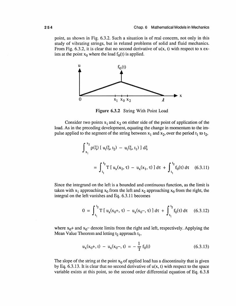
point, as shown in Fig. 6.3.2. Such a situation is of real concern, not only in this study of vibrating strings, but in related problems of solid and fluid mechanics. From Fig. 6.3.2, it is clear that no second derivative of u(x, t) with respect to x exists at the point x0 where the load f0(t) is applied.

u f0 (t)

Figure 6.3.2 String With Point Load

Consider two points x1 and x2 on either side of the point of application of the load. As in the preceding development, equating the change in momentum to the impulse applied to the segment of the string between x1 and x2, over the period t1 to t2,

Since the integrand on the left is a bounded and continuous function, as the limit is taken with x1 approaching x0 from the left and x2 approaching x0 from the right, the integral on the left vanishes and Eq. 6.3.11 becomes

where x0+ and x0- denote limits from the right and left, respectively. Applying the Mean Value Theorem and letting t2 approach t1,

(6.3.13)

The slope of the string at the point Xo of applied load has a discontinuity that is given by Eq. 6.3.13. It is clear that no second derivative ofu(x, t) with respect to the space variable exists at this point, so the second order differential equation of Eq. 6.3.8


cannot apply at point x0• This illustrates that assumptions made for mathematical convenience in deriving equations will often preclude the applicability of the resulting equations to situations that may be of practical interest. This example is provided simply to illustrate that assumptions concerning the regularity properties of functions involved in the problem being studied must be very carefully stated and interpreted .

• In summary, consider a smoothly loaded string, so that candidate deflection func

tions have two continuous derivatives. Also, consider the case in which the string is initially undeformed and at rest; i.e., g(x) = h(x) = 0 in Eq. 6.3.9. The set of admissible deflections can now be described as

D = { u(x, t) E C2: u(x, 0) = ut(x, 0) = 0 for all X in (0, .t) and

u(O, t) = u(.t, t) = 0 for all t ~ 0 } (6.3.14)

Note that functions in D satisfy the differentiability characteristics that are required of the solution, as well as the initial and boundary conditions of Eqs. 6.3.9 and 6.3.10.

A spatial linear operator A may now be associated with the differential equation of Eq. 6.3.8 and the collection of admissible displacements of Eq. 6.3.14,

(6.3.15)

This is called a linear operator since it satisfies the conditions

A ( u + v} = - a2 ( Uxx + v xx } = Au + A v

for all u(x, t) and v(x, t) that have two continuous derivatives with respect to x and for all constants a. The initial-boundary-value problem for motion of a string may now be stated as follows: Find a deflection function u(x, t) in D ofEq. 6.3.14 that satisfies the operator equation

Uu + Au = F(x, t) (6.3.16)

The Transversely Vibrating Membrane

A thin elastic film, called a membrane, is stretched over a closed plane curve r, as shown in Fig. 6.3.3. It offers no in-plane resistance to stretching and distortion. Due to transverse excitation, the membrane may be set into vibratory motion, as if the head of a drum were struck. The objective is to derive the differential equation that governs transverse vibration of the membrane.


u

X

Figure 6.3.3 Transversely Vibrating Membrane

Consider a deformed element of the membrane shown in Fig. 6.3.4 that contains a typical point (x, y) at timet A tension T per unit length acts in the membrane, on the curve C that bounds the element that is imagined cut from the membrane. The tension T is tangent to the membrane and normal to C, since the membrane can support no bending moment and no shear can be supported by the membrane material. In general, the tension can be a function of both space variables and time; i.e., the tension is T(x, y, t).

u

X

Figure 6.3.4 Element of Vibrating Membrane

In this study of small amplitude vibration of the membrane, the angle made by the tangent plane with the x-y plane is small, so squared terms in first derivatives can be ignored. It can be concluded, therefore, that projections of the surface tension onto the x-y plane and the u-axis are

T = T n

T ,.. Tau u an

(6.3.17)


As noted in the preceding, the tension T(x, y, t) can vary over the domain that is bounded by the curve f. Since only transverse vibration of the membrane occurs, there is no movement of the membrane in the x-y plane. This fact implies certain behavior of the tension, which may be investigated by considering the rectangular element of membrane shown in Fig. 6.3.5.

u

X

Figure 6.3.5 Rectangular Element of Membrane

Since there is no motion of the membrane in the x-y plane, the net force on the rectangular element in both the x andy directions must be 0; i.e.,

JYz [ T(x2, y, t) - T(x1, y, t)] dy = 0

Yt (6.3.18)

J x2

[ T(x, Y2• t) - T(x, Yt• t)] dx = 0 xl

Employing the Mean Value Theorem and taking limits as y1 approaches y2 and x1 approaches x2 in Eqs. 6.3.18,

T(x2, y, t) = T(x1, y, t)

T(x, y2, t) = T(x, y1, t) (6.3.19)

This implies that tension is independent of both x andy. Hence it is a function of only t. Since there is no spatial variation of tension in the membrane and no in-plane motion of the membrane, there is no impetus for temporal variation of the tension. Thus, the tension is constant; i.e.,

T(x, y, t) = T (6.3.20)

Equations of motion can now be written for the typical element of membrane shown in Fig. 6.3.4, whose projection onto the x-y plane is a domainS with boundary C. Setting the change in the z-component of momentum of the element from time t1 to ~equal to the


impulse of the z-components of force that act on the element during that period, the integral equation of motion is obtained as

= I ~I T ~~ dC dt + I ~I I f(x, y, t) dx dy dt (6.3.21) tl c tl s

where p(x, y) is the mass per unit area of the membrane and f(x, y, t) is the lateral force per unit area that is applied in the u direction to the membrane.

In order to transform Eq. 6.3.21 into a differential equation, it is assumed that two derivatives of u exist and are continuous. Note that this eliminates the possibility of point or line loads on the membrane. Putting F = Vu in the Divergence Theorem, the boundary integral on the right of Eq. 6.3.21 can be transformed to an integral over the domain S. A manipulation of the integral on the left side ofEq. 6.3.21 yields

f ~I I [ ut(x, y, t2) - ut(x, y, t1) ] t t p(x,y)dxdydt

tl s 2-1

= (' f fs T ( Uxx + Uyy) dx dy dt + f t,'z f f.r dx dy dt (6.3.22)

Employing the Mean Value Theorem yields

= T [ uxx<X, y, t) + uyy(x, y, t)] + f(x, y, t) (6.3.23)

where (i, y) is inS and t1 < t < t2• Taking the limit as the domainS shrinks to the point (x, y) and the time interval [t1, t2] shrinks tot, the differential equation of motion is obtained as

p(x, y) Utt - T ( Uxx + Uyy) = f(x, y, t) (6.3.24)

For a membrane of constant mass distribution over the domain n, p(x, y) is constant and this differential equation reduces to

Un - a2 ( Uxx + Uyy) = F(x, y, t) (6.3.25)

where a2 = T/p and F(x, y, t) = f(x, y, t)/p. This is called the wave equation in two space dimensions for the vibrating membrane.


As in particle equations of motion, it is essential to specify the initial value of the displacement of the membrane and its initial velocity, throughout the domain 0. This results in the initial conditions

u(x, y, 0) = g(x, y)

ut(x, y, 0) = h(x, y) (6.3.26)

in 0. Further, it is required that the displacement of the membrane at the boundary r is 0. This results in the boundary condition

u(x, y, t) = 0 (6.3.27)

on r, for all t ;;::: 0. It may be noted that the differential equation of Eq. 6.3.24, the initial conditions of

Eq. 6.3.26, and the boundary condition of Eq. 6.3.27 form an initial-boundary-value problem similar to that obtained for the vibrating string. The only difference between these problems is the fact that the membrane equation has one additional space variable. As will be noted in later studies of these differential equations, there is considerable similarity in behavior of their solutions. Techniques that can be used to solve the vibrating string problem can also be used to solve the vibrating membrane problem.

Considering the case of motion of a membrane that is initially undeformed and at rest; i.e., g(x, y) = h(x, y) = 0 in Eq. 6.3.26, the collection of admissible membrane deflections for a continuous load can be defmed as

D = { u(x, y, t) E C2(0): u(x, y, 0) = Ut(x, y, 0) = 0 in 0

and u(x, y, t) = 0 on r, for all t } (6.3.28)

A linear operator may be associated with Eq. 6.3.25 and the collection of admissible displacement functions D ofEq. 6.3.28,

(6.3.29)

The initial-boundary-value problem for motion of a membrane may now be stated as follows: Find the deflection function in D that satisfies the operator equation

Uu + Au = F(x, y, t) (6.3.30)

Steady State String and Membrane Problems

Steady state vibration, or harmonic oscillation, and static displacement of strings and membranes represent important classes of applications that arise in mechanics. Consider first harmonic oscillation of the string, in which the time dependence of the displacement function is harmonic; i.e.,

u(x, t) = v(x) sin rot (6.3.31)


where ro is the frequency of harmonic oscillation, or natural frequency of vibration. Substitution of u(x, t) from Eq. 6.3.31 into the homogeneous equation of Eq. 6.3.7; i.e., with f(x, t) = 0, yields

(Tv II + p(x) ro1v) sin rot = 0 (6.3.32)

The boundary condition ofEq. 6.3.10, for all t, is

v(O) sin rot = v(.t) sin rot = 0 (6.3.33)

Since Eqs. 6.3.32 and 6.3.33 must hold for all t, the coefficients of sin rot must be equal to zero. Defining ro2{f =A., an eigenvalue problem is obtained as

- vII = A. p(x) v

v(O) = v(.t) = 0 (6.3.34)

In case pis constant and a is as defined in Eq. 6.3.8, this problem can be solved by noting that the solution of Eq. 6.3.34 is v(x) = sin ( rox/a ). In order that v(.t) = 0, it is necessary that ro-t/a = n1t, where n is an integer. Thus, ron = n1ta/ .t. The eigenvalues and their associated eigenfunctions of Eqs. 6.3.34 are, thus

(6.3.35) ( ) . n1t

VnX = sm-x .t

Similar to the case of a harmonically vibrating string, consider harmonic vibration of a membrane; e.g., vibration of a drum head. As in the case of the string, the displacement is of the form

u(x, y, t) = v(x, y) sin rot (6.3.36)

In order that the boundary condition in Eq. 6.3.27 holds for all t, v(x, y) must satisfy

v(x, y) = 0 (6.3.37)

on r. The homogeneous form of the operator equation of Eq. 6.3.30 now becomes - m2 v(x, y) sin rot- a2V2v(x, y) sin rot= 0, for all t. Defining A.= ro2/a2, the eigenfunction v(x, y) must satisfy the operator eigenvalue equation

Av = -V1v = A.v (6.3.38)

where v(x, y) belongs to the set

DA = { v(x, y) E C2(Q): v(x, y) = 0 on r} (6.3.39)


Note the similarity between the eigenvalue equation of Eq. 6.3.38 for a function v(x, y) and the matrix eigenvalue problem of Eq. 3.1.1. While there are significant technical differences between matrix and differential operator eigenvalue problems, there are also striking similarities.

Having the equations of motion of a membrane, the differential equations that govern equilibrium of a membrane, under a given load f(x, y), may be obtained by noting that the lateral deflection of the membrane is not a function of time; i.e., u = u(x, y). Further, the initial conditions of Eq. 6.3.26 are not meaningful and the boundary condition of Eq. 6.3.27 is independent of time. Therefore, the differential equation

Uxx + llyy = ( 1/T) f(x, y)

in n and the boundary condition

u(x, y) = 0

(6.3.40)

(6.3.41)

on f govern equilibrium of the membrane. These equations form a boundary-value problem of partial differential equations.

The differential equation of Eq. 6.3.40 and the boundary condition of Eq. 6.3.41 can be characterized by the operator equation

Au = -V2u = - ( 1/T) f(x, y) (6.3.42)

D A = { u E C2(.Q): u = 0 on f }

for a continuous load f(x, y).

EXERCISES 6.3

1. Show that the set of admissible displacements D ofEq. 6.3.14 is a vector space. -

2. Define a collection of admissible deflections D for the case g(x) * 0 * h(x) in Eq. 6.3.9. Is this a vector space?

3. Given a function u(x, t) that satisfies Eq. 6.3.9, with g(x) '* 0 '* h(x), show that the change in variables ii(x, t) = u(x, t) - u(x, t) can be employed to reduce the initial conditions to homogeneous form. Obtain the modified equation of Eq. 6.3.8 for ii(x, t).

4. Derive the boundary condition at the right end of the string shown, where the mass of the pin that slides freely in the vertical slot is negligible.

0 ~-


5. Derive the equation of motion of a vibrating string in a viscous medium; i.e., with a resisting force

ou(x, t)

J.L at

in the negative u direction, where J.L is a coefficient of viscosity per unit length of the string.

6. Show that D ofEq. 6.3.28 is a vector space. -

7. Defme the set of admissible membrane deflections D, in case g(x, y) -:F 0 -:F h(x, y), in Eq. 6.3.26.

8. Given a function u(x, y, t) that satisfies Eq. 6.3.26 with g(x, y) -:F 0 -:F h(x, y), show that the transformation u(x, y, t) = u(x, y, t) + ii(x, y, t) can be employed to put the problem in the form of Eq. 6.3.25, with a modified right side and with the domain given in Eq. 6.3.28.

9. For a circular membrane, rewrite Eq. 6.3.25 in terms of polar coordinates.

10. Show that D A of Eq. 6.3.39 is a vector space.

11. Derive a boundary-value problem for equilibrium of a string under the action of a continuous load f(x) and boundary conditions of Eq. 6.3.10.

6.4 HEAT AND DIFFUSION PROBLEMS

In this section, problems of the flow of heat in solids and the flow of gas in porous materials are studied. While these problems have fundamentally different physical properties, it is interesting to note that their mathematical properties are virtually identical.

Conduction of Heat in Solids

Consider a domain .Q in R3 that is bounded by a closed surfacer. Let u(x, y, z, t) be the temperature at a point (x, y, z) at timet. The following important facts govern temperature distribution and heat flow:

(1) If the temperature is not constant, heat flows from regions of higher temperature to regions of lower temperature.

(2) Fourier's Law states that the rate of heat flow is proportional to the gradient of the temperature. Thus, the rate of heat flow v(x, y, z, t) = [ v1 (x, y, z, t), v2(x, y, z, t), v3(x, y, z, t) ]T in an isotropic body is

v =- KVu (6.4.1)

where K > 0 is a constant, called the thermal conductivity of the body.

Sec. 6.4 Heat and Diffusion Problems 263

Let V be an arbitrary region that is bounded by a closed surface S in n. Then, the rate of heat loss from V is

where n is the outward unit normal of S. By the Divergence Theorem, if u(x, y, z, t) is twice continuously differentiable with respect to x, y, and z,

(6.4.2)

The amount of heat in V at a given time is

(6.4.3)

where p is the density of the material of the body and a is its specific heat, both assumed to be constant. Assuming that the temperature u(x, y, z, t) is differentiable with respect to t and using Eq. 6.4.1, the rate of decrease in heat content of V is

(6.4.4)

Since the rate of decrease of heat contained in V must be equal to the amount of heat leaving V per unit of time, from Eqs. 6.4.2 and 6.4.4,

or

for an arbitrary region V in il. Using the Mean Value Theorem,

aput(x, y, z, t) - KV2u(x, y, z, t) = o

(6.4.5)

where (x, y, z) is in V. Letting the volume element V shrink to a typical point (x, y, z), the following differential equation is obtained:

ut - k2V2u = 0 (6.4.6)

where k2 = K/ap. This is known as the heat equation.


In addition to the differential equation of Eq. 6.4.6, the temperature distribution u(x, y, z, t) is determined by the initial temperature distribution within the body and by the temperature maintained at the boundary r of 0. These conditions result in the initial conditions

u(x, y, z, 0) = p(x, y, z)

in 0 and the boundary conditions

u(x, y, z, t) = q(x, y, z, t)

on r, and for all t ~ 0.

(6.4.7)

(6.4.8)

It may be noted that the differential equation ofEq. 6.4.6, the initial condition ofEq. 6.4.7, and the boundary condition of Eq. 6.4.8 form an initial-boundary-value problem that is similar to the problem defined for the vibrating string and vibrating membrane in Section 6.3. The essential difference is that only one time derivative occurs in the differential equation and only the value of the dependent variable u(x, y, z, t) is specified as an initial condition. The fact that only one time derivative of the dependent variable occurs in the differential equation leads to considerably different mathematical properties of the initial-boundary-value problem associated with heat conduction, as compared with the equations of the vibrating string and vibrating membrane. The reasons for these differences in behavior will become more apparent in Chapters 7 and 8.

It is worthy of note that for the study of heat transfer in a bar with one space dimension, or in a plate with two space dimensions, the differential equation ofEq. 6.4.6 maintains precisely the same form, with the spatial differential operator on the right side containing only those space derivatives that are appropriate.

It may be further noted that a steady state temperature distribution in a two dimensional body is independent of time, so the time derivative on the left side of Eq 6.4.6 vanishes and the initial condition of Eq. 6.4.7 is meaningless. The differential equation for steady state temperature u(x, y) is thus

in 0, and the boundary conditions are

u(x, y) = q(x, y)

onr.

(6.4.9)

(6.4.10)

Note that the boundary-value problem formed by Eqs 6.4.9 and 6.4.10 is of the same form as the boundary-value problem for static deflection of a membrane in Section 6.3. The difference is that the membrane differential equation is non-homogeneous and it has homogeneous boundary conditions. This suggests that there is a relation between the steady state temperature distribution in a plane body and the static deflection of a membrane that is stretched over a boundary of the same shape.

To make the analogy between thermal and membrane deflection problems sharper, presume that a C2(0) function u(x, y) that satisfies Eq. 6.4.10 is known. Defining ii(x, y) = u(x, y)- u(x, y), a set of admissible temperatures is obtained as

Sec. 6.4 Heat and Diffusion Problems

D = { ii(x, y) in C2(Q): ii(x, y) = 0 on r}

Then, the operator equation of Eq. 6.4.9 takes on the non-homogeneous form

in n, where the right side of Eq. 6.4.12 is known.

Diffusion of Gas in Porous Materials

265

(6.4.11)

(6.4.12)

If a porous material is non-uniformly filled with a gas, then diffusion of gas occurs from a region of higher concentration to a region of lower concentration. For illustrative purposes, diffusion of a gas along a one dimensional porous material is depicted in Fig. 6.4.1. At any instant of time, the mass per unit volume of gas in a plane normal to the axis of the porous solid is u(x, t).

Figure 6.4.1 Diffusion of Gas in a Porous Medium

For a general porous body Q in R3, with boundary r, the physical relation that governs motion of gas is Fick's law,

q = -DVu (6.4.13)

where u(x, y, z, t) is the mass density of gas, q(x, y, z, t) is the rate of mass flow of gas across a unit area, and the scalar D > 0 is the diffusion coefficient associated with the porous material. The rate of gas flow from a typical volume V in Q, with boundary S is

f f s q Tn dS = - D f f s V u T n dS = - D f f s * dS

where n(x, y, z) is the outward unit normal of S. By the Divergence Theorem,

(6.4.14)

The mass of gas in volume V at a given time is

Q = J J fv Cudxdydz (6.4.15)


where the constant C > 0 is the coefficient of porosity, which is the volume of pores (voids) per unit of volume occupied by the porous material. Thus, the rate of decrease of the mass of gas in V is

dQ JJJ au - - = - c - dx dy dz dt v dt

(6.4.16)

Equating the rate of gas flow out of V, from Eq. 6.4.14, to the rate of decrease in gas content in V, from Eq. 6.4.16,

(6.4.17)

Applying the Mean Value Theorem,

DV2u(x, y, z, t) - Cut(x, y, z, t) = o

where (x, y, z) is in V. Letting V shrink to a typical point (x, y, z) and defining k2 =D/C, the diffusion equation is obtained as

(6.4.18)

If the concentration of gas at the boundary r of Q and the initial concentration of gas in Q are known, then the initial conditions and boundary conditions that must be satisfied by the solution of the diffusion problem are

u(x, y, z, 0) = f(x, y, z), in n u(x, y, z, t) = g(x, y, z), on r, for all t ~ 0

(6.4.19)

Comparing these equations with Eqs. 6.4.6, 6.4.7, and 6.4.8, it is noted that the differential equation and the initial and boundary conditions for the diffusion problem are of precisely the same form as those for the heat conduction problem. Therefore, it can be expected that the mathematical characteristics of gas flow in a porous medium will be identical to those of heat propagation in a solid.

EXERCISES 6.4

1. Formulate an operator equation, with a set of admissible solutions, to represent the initial-boundary-value-problem of Eqs. 6.4.6 through 6.4.8. Is this operator linear?

2. Defme a change of variable in the operator equation of Exercise 1 that makes the set of admissible temperature distributions a linear space. (Hint: Assume that a function that satisfies the initial and boundary conditions ofEqs. 6.4.7 and 6.4.8 is known.)

Sec. 6.4 Heat and Diffusion Problems 267

3. Write the initial-boundary-value problem for the temperature in a rod of length .t that is thermally insulated along its lateral surface, has an initial temperature distribution u(x, 0) = f(x), and for which the ends of the rod are maintained at given temperatures u(O, t) = g(t) and u(.t, t) = h(t).

4. Repeat Exercise 3, but with the ends of the rod insulated; i.e., ux(O, t) = ux(.t, t) = 0.

5. On the lateral surface of a rod, heat is conducted into the surrounding medium at a rate v(x, t) = c [ u(x, t) - T(x, t) ] per unit length of rod, where c is the coefficient of convectivity, T(x, t) is the temperature of the surrounding gas, temperature variation across the cross section of the rod is negligible, and the ends of the rod are insulated. Write the governing initial-boundary-value equations for the system.

6. Derive a heat equation for a medium in which a chemical reaction generates heat at a rate Q(x, t) heat units per unit of mass of material.

7. Derive a heat transfer equation in a cylindrical body, where u = u(r, z, t), u(r0, z, t) = u(r, 0, t) = u(r, .t, t) = 0, and u(r, z, 0) = f(r, z).

X

y u=O

8. Write the equation for diffusion of a gas in a cylindrical volume of porous material, as shown in Fig. 6.4.1, where uniform concentration of gas across each cross section is assumed. The initial concentration is u(x, 0) = f(x) and the ends of the volume are sealed; i.e., ux(O, t) = ux(.t, t) = 0.

9. Repeat Exercise 8, but with the ends of the column semi-permeable; i.e., the rates of gas flow out of the tube are

q(O, t) = K [ u(O, t) - v(t) ]

q(.t, t) = K [ u(.t, t) - v(t) ]

where v(t) is the gas concentration outside the porous medium.


10. Write the diffusion equation for a column of porous material in which a chemical reaction generates gas at a rate Q(x, t) and gas flows out of the ends according to the law

q(O, t) = - D u(O, t)

q(.t, t) = Du(.t, t)

11. In case Q(x, t) does not depend on time, write a steady state equation of flow for the problem in Exercise 10.

12. Define a relationship between the thermal and diffusion constants and the initial conditions so that the temperature in Exercise 4 is identical to the gas density in Exercise 8.

6.5 FLUID DYNAMICS

A major topic in the field of continuum mechanics is fluid and gas dynamics. The basic equations that govern flow of fluids and gases are derived in this section, to include special cases that are of interest in applications.

Dynamics of Compressible Fluids

Fluid dynamics is considerably different, in a physical sense, from the dynamics problems discussed in Section 6.3. The fundamental difference is that an ideal fluid cannot resist shearing stress. That is, continued deformation of a fluid can occur such that rates of shearing strain are maintained and large deformations occur in the continuum. Thus, it is natural to study the flow of fluids from the point of view of determining a velocity distribution in the continuum, rather than determining displacements of individual fluid particles, as is done in vibration problems.

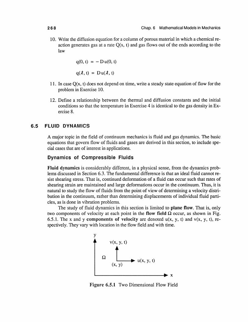
The study of fluid dynamics in this section is limited to plane flow. That is, only two components of velocity at each point in the flow field Q occur, as shown in Fig. 6.5.1. The x andy components of velocity are denoted u(x, y, t) and v(x, y, t), respectively. They vary with location in the flow field and with time.

y

v(x, y, t)

L u(x,y,t) (x, y)

~----------------------~ X

Figure 6.5.1 Two Dimensional Flow Field

Sec. 6.5 Fluid Dynamics 269

In addition to determining the velocity of the flow field, fluid density and pressure within the flow field must also be determined. Density of the fluid will be denoted by p(x, y, t) and pressure in the fluid will be denoted by p(x, y, t). Finally, an external force may act on each unit of mass in the flow field. The components of this force will be denoted Fx(x, y, t) and Fy(x, y, t). Such forces may arise from gravitational effects or from interaction of the fluid with some other field of influence, such as magnetic or electrostatic fields that may have some effect on the fluid

Consider a typical element of fluid in the flow field, as shown in Fig. 6.5.2, that occupies an area S c n and has boundary C. Consideration is limited here to ideal fluid, in which no viscosity exists. That is, only a pure pressure exists in the fluid and no shear is supported along any boundary in the flow field. Assuming that the pressure p is differentiable, the components of the resultant force that act on the element of fluid in S in the x and y directions are

-Jcpnxdr + JJsPFxdxdy =-JJs~ dxdy + JJsPFxdxdy

- J c pny dr + J J s pFy dx dy = - J J s ~~ dx dy + J J s pFy dx dy

(6.5.1)

where the Divergence Theorem has been used to transform boundary integrals over C to integrals over S.

y

~----------------------~ X

Figure 6.5.2 Element in Flow Field

For the set of mass points in S of Fig. 6.5.2, the components of the resultant applied force in Eq. 6.5.1 must equal the time derivatives of the corresponding components of momentum. The components of momentum of fluid in S in the x and y directions are

J Js pudxdy

(6.5.2)


Using the material derivative of Section 6.2 to compute the time rate of change of momentum and equating the results to the corresponding forces in Eq. 6.5.1,

J J s [ ( pu )t + ( pu2 )x + ( puv )y + Px - pFx] dx dy = 0

J J 8 [ ( pv )t + ( puv )x + ( pv2 )y + Py - pFy ] dx dy = 0

for all regions Sin the flow field. Applying the Mean Value Theorem and letting S shrink to a point, the equations of fluid motion are obtained in the form

( pu )t + ( pu2 + p )x + ( puv )y = pFx

( pv )t + ( puv )x + ( pv2 + p )y = pFy (6.5.3)

Recall from Eq. 6.2.14 of Section 6.2, the condition of conservation of mass is

Pt + ( pu )x + ( pv )y = 0 (6.5.4)

This is called the continuity equation and states that mass is neither created nor destroyed in the flow field. The equations of fluid dynamics of Eqs. 6.5.3 and 6.5.4 can be written in divergence form; i.e.,

[pu] [pu2+ p] [ puv ] [PFx] pv + puv + pv2 + p = pFY

P t pu x pv y 0

(6.5.5)

where u(x, y, t), v(x, y, t), p(x, y, t), and p(x, y, t) are unknowns. This form of the nonlinear equations of fluid motion is the direct result of conservation laws used in their derivation.

In order to extract physically meaningful conclusions from the two dimensional equations of fluid dynamics, it is occasionally helpful to write Eq. 6.5.3 in a slightly different form. Carrying out the differentiation in Eq. 6.5.3, employing the continuity equation of Eq. 6.5.4, and multiplying by 1/p(x, y, t),

1 Ut + UUx + VUy + - Px = Fx p

(6.5.6) 1

v t + uv X + VVy + - p = F p y y

In order to proceed further, it is necessary to introduce a relation between p and p. Without delving into the theory of thermodynamics, the case of constant entropy


(isentropic flow) is treated, for which there exists an algebraic relation p = f(p ), called the equation of state. An important special case that is valid for gases is the isentropic gas law

p = ApY (6.5.7)

where A is a constant and y is the ratio of specific heats of the ideal gas being studied. The condition A = constant along a particle path can be enforced by writing

dA dt = A1 + uAx + v Ay = 0 (6.5.8)

Using Eq. 6.5.7 to eliminate A from Eq. 6.5.8, a partial differential equation is obtained as

(6.5.9)

For gases, the ratio of specific heats y is not much greater than 1. In particular, y= 7/5 = 1.4 for air. Consequently, Eq. 6.5.9 plays a significant role in most problems of aerodynamics. On the other hand, the density for liquids is often virtually independent of pressure. Thus, in hydrodynamics, Eq. 6.5.7 can be replaced by the more elementary equation of incompressibility

p = constant (6.5.10)

and Eq. 6.5.9 can be omitted. A common condition that must be satisfied at a solid-fluid boundary r of the

flow field n is that the fluid does not penetrate the boundary and that no gaps occur between the boundary and the fluid. If the boundary is stationary, this condition may be stated as

on r; i.e., that the component of the fluid velocity normal to the boundary must be zero, where nx(x, y) and ny(x, y) are direction cosines of the normal to the boundary.

When the boundary is in motion, the fluid velocity component normal to the boundary must equal the normal component of velocity of the boundary. Letting u(x, y) represent the normal velocity of the boundary, the boundary condition becomes

onr.


lrrotational, Incompressible, and Steady Isentropic Flows

Note that the equations of motion for a fluid are non-linear in the variables of the problem. This fact tends to make the study of fluid dynamics considerably more complicated than that of vibrating strings and membranes, whose governing equations are linear. There are, however, special cases of fluid dynamics that can be treated by specialized techniques, which is the focus of the remainder of this section.

Circulation (Potential Flow): For any closed curve C in an isentropic flow field n that encloses a region S, as in Fig. 6.5.2, a quantity called the circulation associated with the curve is defined as the integral of the projection of the velocity vector onto the tangent to the curve,

(6.5.11)

where the integral overS is obtained by applying Green's theorem. Using the material derivative to compute the time derivative of ~. after some manipulation,

!: = J JS {;X ( Vt + UVx - UUy]

+ ;y (- Ut + VVx - VUy]} dx dy

Substituting from Eq. 6.5.6, with external forces equal to zero, yields

d~ = J J { ~ [ - .!_ p - vv - uu J dt sax pY Y Y

+ ;Y [ ~ Px + UUx + VVx J } dx dy

Using Green's theorem to transform this to a boundary integral and manipulating,

!: = - ~ J c [ d( u2 ) + d( v2 ) ] - J c ~ ( Px dx + Py dy )

=- fc ~ = 0

(6.5.12)

(6.5.13)

which follows since the first integrand is a total differential and since an equation of state such as p = f(p) determines p as a function of p. Thus, in the absence of external forces, the circulation in the flow field is invariant with time. If the flow starts without rotation, then ~ = 0 for all time; i.e., irrotational flow occurs throughout its time history.


LetS in Fig. 6.5.2 shrink to a typical point (x, y) in Eq. 6.5.11 and use the Mean Value Theorem to conclude that ()v(x, y, t)/i)x = ()u(x, y, t)/i)y. Thus the differential form u(x, y, t) dx + v(x, y, t) dy is exact, at each timet. Theorem 6.2.1 then implies that there exists a function <j>(x, y, t), called a velocity potential, such that

aq, ()y = v

(6.5.14)

Inserting Eq. 6.5.14 into Eq. 6.5.6, premultiplying the first equation by dx and the second by dy, adding, and integrating over a curve C that is not necessarily closed yields

J C [ (<I> tx + UUx + VVx + ~ Px) dx

+ (<I> ty + UUy + VVy + ~ Py) dy J = 0

providing there is no external force. With some rearrangement, this equation becomes

(6.5.15)

where H is a function of time alone. This equation is called Bernoulli's Law, or Bernoulli's equation. Along with a state equation p = f(p), it allows computation of the pressure field, once the velocity potential is known. In this sense, irrotational isentropic fluid dynamics problems are reduced to determination of the velocity potential that satisfies the continuity equation of Eq. 6.5.4, since the equations of motion of Eq. 6.5.6 are identically satisfied.

Incompressible Potential Flow: In case an isentropic, irrotational flow is also an incompressible flow, which is a good approximation for liquids, the density p is constant and Eq. 6.5.4 reduces to the familiar Laplace's Equation for the velocity potential <j>(x, y); i.e.,

V2q, = <l>xx + <!>yy = 0

Example 6.5.1

(6.5.16)

Consider the steady; i.e., time independent, flow around a cylinder (such as a bridge pile) in a flow field 0 that is rectilinear at infinity, as shown in Fig. 6.5.3. The flow velocity at infinity is taken as u leo= 1 and v loo = 0, so that at infmity, <j>(x, y) = x. At the boundary r of the cylinder, the normal velocity of fluid flow must be zero. This simply reflects the fact that the normal derivative of the velocity potential on r is


zero. This steady flow field is governed by the following boundary-value problem for the velocity potentialcp(x, y):

V2cp = 0, in n

()cp=O onr dn '

cploo =X

y

Figure 6.5.3 Steady Flow Around a Cylinder

(6.5.17)

• Steady Isentropic Flow: Regardless of whether the flow is irrotational, all time

derivatives in the equations of motion vanish in a case of steady flow. In this case, the continuity equation of Eq. 6.5.4 implies the existence of another potential function, called a stream function 'I' = 'JI(x, y), such that

pu = ~ (6.5.18)

pv = -~

in n. The time rate of change of the stream function along the path swept out by a particle is

1 'If = 'lfxU + 'JiyV = p ( 'l'x'l'y - 'Jiy'l'x) = 0 (6.5.19)

Thus, curves 'JI(x, y) = constant follow fluid particle paths, so they are called stream lines. A set of stream lines is shown in Fig. 6.5.3.


One-dimensional Isentropic Flow: In case of flow only in the x direction, without external forces, the equations of motion and continuity reduce to

1 Ut + UUx + p Px = 0

The isentropic equation of state for the fluid is

p = Ap"f

where A is a constant. Defining a new parameter c as

c2 = dp = Ayp"f-1 dp

which depends only on p, p may be eliminated from Eq. 6.5.20, to obtain

(6.5.20)

(6.5.21)

(6.5.22)

(6.5.23)

(6.5.24)

Steady, Isentropic, Irrotational Flow: For the steady isentropic flow case, Eq. 6.5.22 provides the equation of state, which may be substituted directly into Bernoulli's equation of Eq. 6.5.15, with <l>t = 0, to obtain

.!. ( u2 + v2) + Ayp"f-1 = H 2 y-1

(6.5.25)

where H is a constant. Differentiating this equation first with respect to x and then with respect to y allows development of the formulas

Px = - p2 ( u<l>xx + v<l>yx ) c

Writing Eq. 6.5.4 in terms of the velocity potential yields

Expanding the derivatives and substituting from the preceding equations, a second order partial differential equation is obtained as


(6.5.26)

Equation 6.5.26 is a special case of the non-linear equations of fluid flow. This equation will be important later in demonstrating flow characteristics as a function of the velocity of flow of the fluid.

Propagation of Sound in Gas

Consider a gas at rest that is subjected to a small initial excitation. Since only small motion of particles in the gas occurs, the process proceeds isentropically and the equation of state of Eq. 6.5.22 holds. Denoting the pressure and density in still gas as Po and p0, a new quantity s(x, t) is defined, called the compression,

s = ( P - Po ) I Po or (6.5.27)

p = Po ( 1 + s)

For small amplitude oscillations (sound waves) in the gas, the compression should be small and second order terms involving this variable can be neglected.

Employing the approximations

( pu )x = PxU + PUx "" PoUx

1 1 (6.5.28)

p Px "" i); Px

and ignoring product terms that involve gas flow velocities and their derivatives, Eqs. 6.5.4 and 6.5.6 become

1 ut + Po Px = 0

(6.5.29)

Pt + PoUx = 0

where no external force is applied. Employing Eq. 6.5.27, the equation of state of Eq. 6.5.22, and Eq. 6.5.23, the reduced equations are obtained as

u1 + c5sx = 0 (6.5.30)

where c0 denotes the value of c at the air density Po in still gas. Differentiating the first of Eqs. 6.5.30 with respect to x and the second with respect

to t and substituting the second into the first, the second order differential equation for the

Sec. 6.6 Analogies (Physical Classification) 277

compression s(x, t) is

(6.5.31)

It should be recalled that Eq. 6.5.31 holds only for small vibratory motion; i.e., propagation of sound in a gas, commonly known as the equation of acoustics. Note also that this is the same differential equation that governed the vibration of a string, so it can be expected that the same type of physical behavior will be associated with string vibration as occurs in propagation of sound in gas.

EXERCISES 6.5

1. For a static fluid in which x is horizontal and y is vertical, u = v = 0, Fx = 0, and Fy =-g. Reduce the general equations of motion to represent this static case, called hydrostatics.

2. If the static fluid in Exercise 1 is of constant density; e.g., water, derive an expression for pressure as a function of depth.

3. Extend the equations of motion and continuity to three space dimensions and time.

4. Which of the following are velocity potentials for incompressible irrotational flow:

(a) <1> = x + y

(b) <I> = x2 + l (c) <1> = sin ( x + y)

(d) <1> = In x

5. Use the results of Exercise 3 to define the flow field of an incompressible fluid that is spinning steadily counterclockwise with a vertical cylinder, about its axis, at angular speed ro rad/sec. Use the fact that u =-roy, v = rox, and w = 0, where w is the z component of velocity. Use the equations of motion to find the pressure p as a function of x, y, and z. Finally, put p =constant to find the shape of the free surface of the fluid.

6.6 ANALOGIES (PHYSICAL CLASSIFICATION)

As may be noted for the very different physical problems treated in the preceding sections, the same form of partial differential equations arise; with only variations in the form of the non-homogeneous terms in the differential equations, boundary conditions, and initial conditions. In some cases, the differential equations, boundary conditions, and initial conditions are identical, even for problems that have considerably different physical signif-


icance. Therefore, analogies can be considered in a mathematical sense, and even in a physical sense when experimentation in one problem may be readily performed but may be difficult in an analogous problem. To illustrate this point, four different forms of second order partial differential equations are shown in Table 6.6.1 and the physical problems that are described by each form of differential equation are tabulated.

Table 6.6.1 Analogous Physical Problems

u11 - a2V2u = f ut - k2V2u = f V2u = f -V2u = crl -u a2

Vibrating String Conduction of Heat Static Deflection of Harmonic Vibrating in Solids String String

Vibrating Static Deflection of Membrane Membrane

Sound Diffusion of Gas in Steady State Tern- Harmonic Vibrating Propagation a Porous Medium perature Distribution Membrane in Gas in Solids

Steady lncompres-sible, Irrotational Flow of Fluids

First note a fundamental difference between problems governed by Laplace's equation, in the third column, and those governed by the wave and heat equations in the first and second columns. Laplace's equation is associated with static or steady state (time independent) problems. It will be noted in Chapters 7 and 8 that very different mathematical and physical properties are associated with the solution of static problems, as compared with dynamics problems. Finally, as noted in the fourth column, harmonic vibration is governed by an eigenvalue problem.

Within the class of dynamics problems, the only essential difference between the wave and heat equations is the order of the highest time derivative that appears in the differential equation. While in some ways the solutions of these time dependent problems are similar, fundamental differences in the two classes will be noted in Chapters 7 and 8.

The model problems selected from different fields of mechanics in this chapter illustrate techniques that may be used to derive the partial differential equations of continuum behavior and to show that there are a limited number of basic types of differential equations that arise in the study of second order partial differential equations. Such problems and associated equations are commonly called Equations of Mathematical Physics. They are used to study the fundamental properties of differential equations, to provide insight into techniques that can be used for the study of more complex problems. When more complex problems arise, algebraic messiness of the governing equations involved

Sec. 6.6 Analogies (Physical Classification) 279

will occur. It will be found, however, that many of the fundamental features found in the model problems derived in this chapter are present in more general and complex problems. It is essential, therefore, to study the second order differential equations associated with these model problems, for the purposes of developing solution techniques and physical and mathematical insights into techniques for solving partial differential equations of mechanics.

A second key point that must be noted in this discussion is that the problems highlighted in Table 6.6.1 are linear and, as was noted in Section 6.5, problems such as those in fluid dynamics are governed by nonlinear differential equations. This is also true of the field of finite elasticity and other fields of nonlinear mechanics. While nonlinear differential equations arise naturally in general continua, no uniformly applicable solution technique is known. Solution techniques for the various types of nonlinear continua must, therefore, be studied on an ad-hoc basis. No attempt is made in this text to be complete in treatment of such nonlinear problems. Rather, concentration is on development of broadly applicable solution techniques and analysis methods that can be employed in studying problems that arise in mechanics and to provide experience and a stepping off point for the study of methods for solving the more complex problems of mechanics.

6 MATHEMATICAL MODELS IN MECHANICSuser.engineering.uiowa.edu/~kkchoi/Chapter_6.pdf6 MATHEMATICAL MODELS IN MECHANICS ... Theorem 6.1.2 (Green's Theorem). If real valued functions P(x1,

Documents