6. Chapter 6 Acquisition-geometry Survey Design

Chapter 6 Acquisition-geometry Survey Design

Introduction

Biondi (2007, p. 1) writes, “The main goal of conventional acquisition design is to obtain an adequately and regularly sampled stacked cube that can be imaged accurately by poststack migration . . . . However, in common acquisition geometries, sampling of the offset axes may be inadequate when the data require prestack processing that is more sophisticated prestack processing than simple stacking.” It could not be stated more clearly that the first imaging phase is survey design. That phase does not require the highest mathematical skill, but its consequences can be dramatic. There is an inter-esting contradiction between these two sentences in Biondi (2007), which are within the same paragraph of his text. It does not seem difficult to obtain an adequately sam-pled stacked cube, but how can common acquisition geometries offer inadequate sam-pling of the offset axes? That contradiction is very much like the “original sin” of survey design.

In the 3D survey-design workshop held at the 61st EAGE Conference and Exhibi-tion in 1999, Kees Hornman and Gijs Vermeer invited five specialists to present their solutions to the same survey-design problem. Five totally different solutions were pro-posed. All five designers had the same understanding of the technical side of the prob-lem, but they did not share the same understanding of its economic side. One designer proposed the best technical solution, ignoring all economic aspects, and another came with a proposal that focused on winning the bid. As could be expected, the solutions were very different.

Three-dimensional survey design has more to do with the art of compromise than with the science of wave propagation. In fact, the major borrowing that survey design makes from science is the necessity of adequately sampling the wavefield (the Shannon–Nyquist theorem tells us that adequate sampling requires two samples per wavelength). In Chapter 3, I indicated that although signal wavelengths usually are larger than a few tens of meters, noise wavelengths have a bad tendency to be significantly shorter. Rached (2007) observes an 8-m wavelength in a ground roll in the Middle East. Off-shore, low-velocity waves propagate along the streamer with wavelengths in an even shorter range. Those short wavelengths are the main reason why source and receiver arrays were and still are used widely.

In this chapter, I will rephrase Biondi’s guideline mentioned above (Biondi, 2007, p. 1) to make it more general and include a discussion of noise. The processing geophysi-cist generates an image of the underground from seismic data collected by his acquisi-tion colleague. Survey design consists of defining the conditions for those data to lead to an adequate image.

Distinguished Instructor Short Course • 129

Dow

nloa

ded

01/1

7/13

to 1

92.1

59.1

06.2

00. R

edis

trib

utio

n su

bjec

t to

SEG

lice

nse

or c

opyr

ight

; see

Ter

ms

of U

se a

t http

://lib

rary

.seg

.org

/

To construct a good seismic image, the reflected wavefield on a surface surrounding the imaging area must be known. Imperfection of the seismic image essentially results from three causes: (1) nonproportionality between the motion of the ground (or the pressure in the vicinity of the ocean surface) and the reflected wavefield (presence of noise), (2) inadequate sampling and limited size of the measurement surface, and (3) measurement and processing errors.

The next section discusses the first cause — nonproportionality. That is followed by a section on signal constraints, discussing the second cause, even though inadequate sampling also affects noise (often more than signal). The third section, on errors, will use 4D seismic to underscore the importance of error management. I will end with a fourth section on parameter selection.

Noise constraints

In early survey-design papers and lectures, the discussion of noise often was re-stricted to direct ground roll. Sometimes, scattering of the ground roll was considered. Ambient noise (i.e., noise independent from the source) was ignored. It was assumed (and the assumption probably was well justified) that the dynamite charge was large enough to reject ambient noise as negligible. Doubling the dynamite charge might not have a dramatic effect on survey cost, but multiplying the sweep length by a factor of four does. Therefore, ambient noise cannot be ignored.

Source-generated noise

It is convenient to start with the 2D problem. There are several ways to separate reflected body waves, whose arrival time follows a hyperbolic function from ground roll with linear arrival times. Two of those ways (spatial filtering in the field and velocity filtering in the processing center) are combined in most land-seismic imaging projects. They both use the same property of ground roll in the time-offset domain to show an apparent velocity significantly slower than that of reflections.

There are other ways to separate the body waves, particularly polarization filtering, which uses the fact that ground roll essentially consists of Rayleigh waves with elliptical polarization, although body waves are polarized linearly. Polarization filtering requires the use of three-component (3C) receivers to record the full particle motion. I shall not discuss those techniques, but one must keep in mind that when they are successful, they can relax the sampling constraints imposed by noise.

Spatial filtering in the field: Array forming

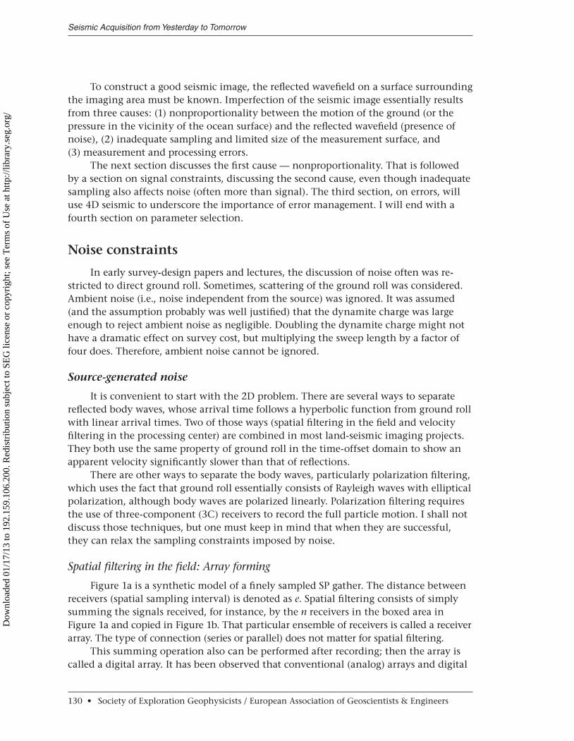
Figure 1a is a synthetic model of a finely sampled SP gather. The distance between receivers (spatial sampling interval) is denoted as e. Spatial filtering consists of simply summing the signals received, for instance, by the n receivers in the boxed area in Figure 1a and copied in Figure 1b. That particular ensemble of receivers is called a receiver array. The type of connection (series or parallel) does not matter for spatial filtering.

This summing operation also can be performed after recording; then the array is called a digital array. It has been observed that conventional (analog) arrays and digital

Seismic Acquisition from Yesterday to Tomorrow

130 • Society of Exploration Geophysicists / European Association of Geoscientists & Engineers

Dow

nloa

ded

01/1

7/13

to 1

92.1

59.1

06.2

00. R

edis

trib

utio

n su

bjec

t to

SEG

lice

nse

or c

opyr

ight

; see

Ter

ms

of U

se a

t http

://lib

rary

.seg

.org

/

arrays are practically identical. The result of such a summation is represented in Figure 1c, where it can be seen that ground-roll amplitude has been reduced signifi-cantly, although reflection amplitudes are conserved (except on the larger offsets). It is convenient to represent the summation of n sensors in an array

Array wf

= Â+ +

( , ), , , ... ,

t xx x e x e x1 1 1 2 2

(1)

as a convolution of the continuous wavefield wf(t, x) by a comb with n teeth followed by decimation:

Array decim wf rec= *( ( , ) ( , ), ).t x m e n (2)

Here, array represents the resulting data, decim(x, n) represents the operation of decimation of vector x by a factor n, and rec(m, e) represents an m-tooth comb filter with a tooth interval equal to the receiver interval e.



Offseta)

b) c)

0

0.2

0.4

0.6

0.8

1.0

1.2

1.4

1.6

0

0.2

0.4

0.6

0.8

1.0

1.2

1.4

1.65 10 15

0

0.2

0.4

0.6

0.8

1.0

1.2

1.4

1.6

0 10

e

eE1 E2

20 30 40 50 60 70 80

Tim

e

Reflection

Ground roll

Figure 1. The receiver array. (a) 2D seismic gather in the offset time domain. The trace interval is e. This gather is associated with a comb of tooth interval e. (b) Group of n traces to be summed together to constitute a receiver array. The “seismic length” of the array is E1 = ne. (c) Same gather as in part (a) after array forming and decimation. The new tooth interval is E2. Used by permission of CGGVeritas.

Dow

nloa

ded

01/1

7/13

to 1

92.1

59.1

06.2

00. R

edis

trib

utio

n su

bjec

t to

SEG

lice

nse

or c

opyr

ight

; see

Ter

ms

of U

se a

t http

://lib

rary

.seg

.org

/

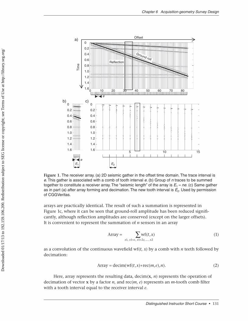
If those two expressions are indeed equivalent mathematically, the Fourier transform of the second expression offers a convenient representation of the array property. Such a representation is given in Figure 2. The array effect on the data is seen in the dashed curve obtained before the data have been decimated. The effect of decimation (which is a resampling) is seen in the gray curve. The difference between the dashed curve and the gray curve at wavenumbers lower than 0.01 m−1 (Nyquist wavenumber of the decimated data) is aliased energy in the decimated data. It shows a weakness of the spatial array filters. They are used as antialias filters to allow spatial resampling, but they are not perfect antialias filters.

In this particular case, the noise spectrum is maximal at wavenumbers significantly higher than the Nyquist wavenumber 1/2E2 = 0.01 m−1 (see Figure 1

for definitions of E1 and E2). The array filter does not fully attenuate that noise, which folds back around the Nyquist wavenumber in the resampling process. It turns out that this aliasing situation is not necessarily a significant problem. Array-filter efficiency is highest in the wavenumber region around 1/E1. After resampling from the geophone interval e to the station interval E2, this region folds back around the Nyquist wavenum-ber kN = 1/2E2 into 1/E1 − 1/E2. If E1 = E2, aliased noise will be attenuated in the wave-number area around zero, which is precisely the area where most of the signal is found. Therefore, it is recommended to select an array length equal to station interval.

Another solution is to record the signals of individual geophones rather than using field arrays. In this case, signal and noise are separated after recording, using numerical techniques that are more flexible and potentially more efficient. Recording individual geophone signals avoids problems associated with field arrays, such as intra-array statics (static differences between various elements of the array) and residual moveout, which is the normal-moveout (NMO) difference among the various elements of the array.

2D stack array

The term stack array, introduced by Anstey (1986), refers to the fact that the com-mon-midpoint (CMP) stack can be viewed as a spatial filter in the same manner as a source or receiver array. Seismic traces constituting a given CMP can be represented in the source-receiver offset domain in the same manner as individual sensors constituting a receiver array. Summing is performed numerically instead of electrically. In two dimensions, offset is taken as the modulus of the source-receiver vector. Therefore, it is

00

0.1

0.2

0.3

0.4

0.5

Tim

e (s

) 0.6

0.7

0.8

0.9

0.1

0.01 0.02

Filtered and decimated k-spectrum

Filtered k-spectrum

Original k-spectrum

Theoretical response

0.03Wavenumber (m–1)

0.04 0.05 0.06

Figure 2. Spatial filtering by the receiver array. The black line is the theoretical response of a six-element array with an 8.33-m interval. The dotted line is the wavenumber transform of the noise. The dashed line is the wavenumber transform of noise convolved by the array. The gray line is the wavenumber transform of deci-mated noise convolved by the array. Used by permission of CGGVeritas.



Dow

nloa

ded

01/1

7/13

to 1

92.1

59.1

06.2

00. R

edis

trib

utio

n su

bjec

t to

SEG

lice

nse

or c

opyr

ight

; see

Ter

ms

of U

se a

t http

://lib

rary

.seg

.org

/

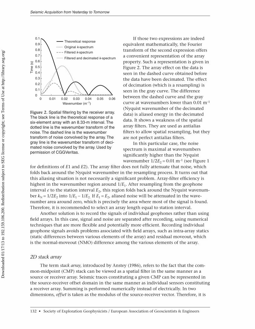
assumed implicitly that waves propagate with the same velocity forward and backward. Figure 3 shows the optimal 2D geometry, which often is called stack-array geometry. It should honor the following conditions:

Shotpoints (SP) should be recorded with receivers in the front and rear • (split-spread).Source and receiver intervals should be the same.• The SP should be located halfway between receivers.• The receiver interval should be • n (number of sensors) times the sensor interval.

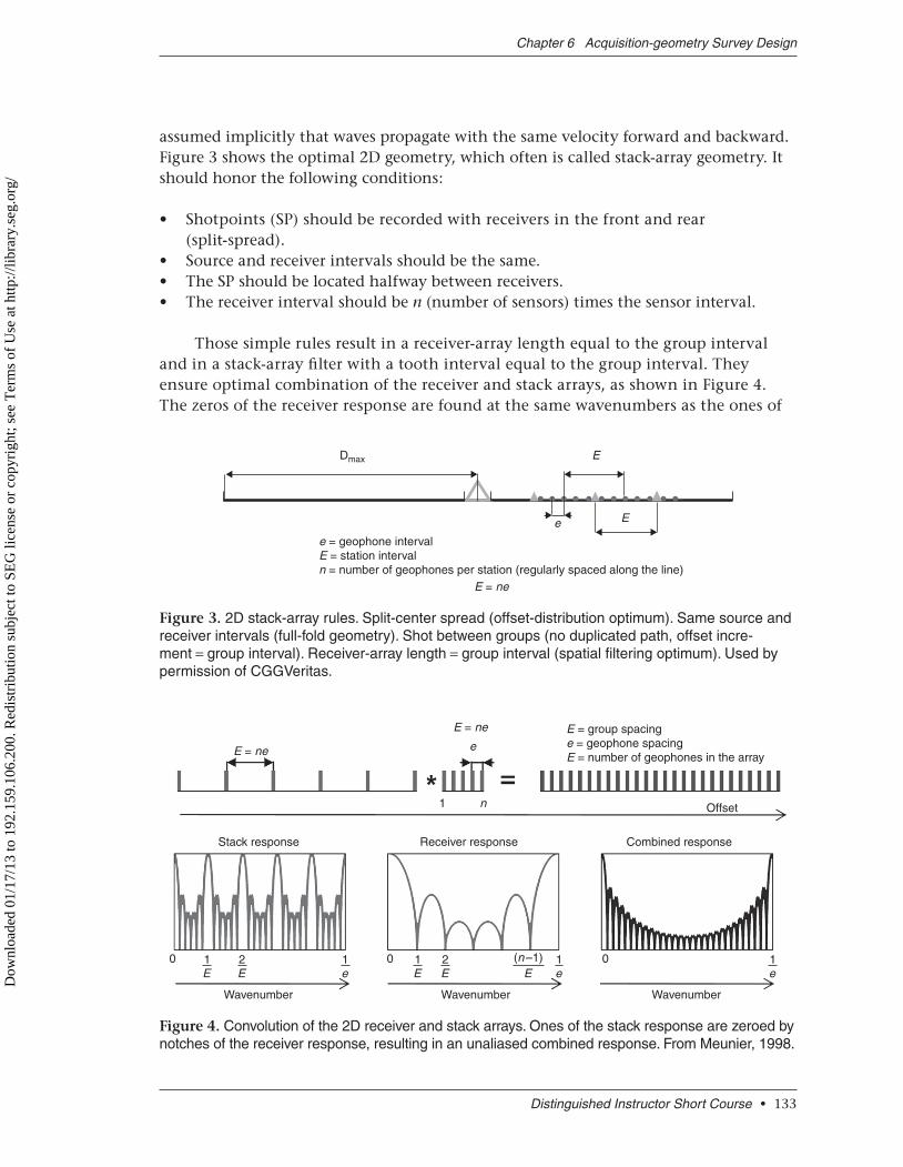
Those simple rules result in a receiver-array length equal to the group interval and in a stack-array filter with a tooth interval equal to the group interval. They ensure optimal combination of the receiver and stack arrays, as shown in Figure 4. The zeros of the receiver response are found at the same wavenumbers as the ones of



Dmax E

E

E = ne

e

e = geophone intervalE = station intervaln = number of geophones per station (regularly spaced along the line)

Figure 3. 2D stack-array rules. Split-center spread (offset-distribution optimum). Same source and receiver intervals (full-fold geometry). Shot between groups (no duplicated path, offset incre-ment = group interval). Receiver-array length = group interval (spatial filtering optimum). Used by permission of CGGVeritas.

E = ne e

Stack response

0 1E

0 0(n –1)

Wavenumber Wavenumber Wavenumber

Receiver response Combined response

E = ne

1 Offsetn

E = group spacinge = geophone spacingE = number of geophones in the array

1E

2E

2E E

1e

1e

1e

Figure 4. Convolution of the 2D receiver and stack arrays. Ones of the stack response are zeroed by notches of the receiver response, resulting in an unaliased combined response. From Meunier, 1998.

Dow

nloa

ded

01/1

7/13

to 1

92.1

59.1

06.2

00. R

edis

trib

utio

n su

bjec

t to

SEG

lice

nse

or c

opyr

ight

; see

Ter

ms

of U

se a

t http

://lib

rary

.seg

.org

/

the stack response. The resulting array is effective up to the inverse of the sensor interval. If the sensor interval is chosen to sample the noise wavefield properly, that combination will result in an effective attenuation of the noise. Figure 5 illustrates that property. In Figure 5a, a full-fold stack honoring the stack-array rules of Fig-ure 3 is compared with a half-fold stack (Figure 5b), in which every second SP is missing. Amplitude distortions can be seen on the half-fold stack, corresponding to ground roll leaking through the stack.

A property of the receiver-array response seen in Figure 4 is used to define the geophone interval. That response can be considered as a reject filter between the first and last zero of the response between wavenumbers 1/ne and (n − 1)/ne. Noise with wavenumbers outside that range will leak through the array. For example, with a five-element string, the highest wavenumber of the noise should be less than (5 − 1)/5 = 80% of the inverse geophone interval. Even though the number five is somewhat arbitrary, this statement is equiva-lent to

e ≤ 0 8. ,minl (3)

where e is the geophone interval and λmin is the shortest noise wavelength. If that condition is met and if the stack-array rules are applied, ground-roll leakage in the stack should be minimal. Note that the actual receiver interval does not appear directly in this condition. As shown in Chapter 3, the optimal receiver interval for ambient-noise attenuation is also 80% of the shortest ground-roll wavelength. The consistency of those two

results is not surprising because it was assumed in Chapter 3 that ground roll is the dominant component of ambient noise.

Ongkiehong and Askin (1988) present stack-array properties quite elegantly. In particular, they discuss a notable difference between the sum in a receiver array and the CMP stack. The former is a straight addition, and the latter is not. In particular, NMO always is applied before CMP stack. Ongkiehong and Askin (1988) show that NMO, designed to make apparent velocity of reflections infinite, also makes the apparent ve-locity of noise slightly faster. Consequently, the harmony of the combination essentially survives NMO. However, there are two obvious limitations to this theory. First, it assumes a 2D world with no possible wave scattering. It is well known how wrong that assump-tion can be. Second, it assumes plane waves. Very often, that is not the case. Three-di-mensional stack-array theory does not need the first assumption, but it does need the second one.



Full folda)

CMP number

0.0

0.5

Tim

e (s

) 1.0

1.5

2.0

b)

CMP number

Half fold0.0

0.5

Tim

e (s

) 1.0

1.5

2.0

Figure 5. Comparison of (a) full-fold stack honoring the stack-array recommendations and (b) half-fold stack. Used by permission of CGGVeritas.

Dow

nloa

ded

01/1

7/13

to 1

92.1

59.1

06.2

00. R

edis

trib

utio

n su

bjec

t to

SEG

lice

nse

or c

opyr

ight

; see

Ter

ms

of U

se a

t http

://lib

rary

.seg

.org

/

3D stack array

From a theoretical point of view, the extension of the 2D theory to three dimen-sions is not exactly straightforward. Source and receiver lines become source and receiver grids, and 1D arrays (combs) become 2D arrays (brushes). The source-receiver offset no longer can be considered a scalar as in two dimensions. It is a vector, with an azimuth ranging over 360°.

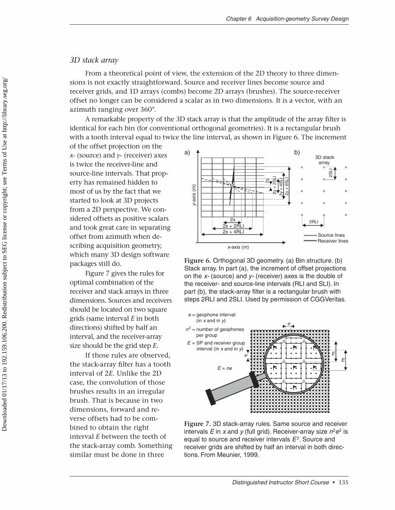
A remarkable property of the 3D stack array is that the amplitude of the array filter is identical for each bin (for conventional orthogonal geometries). It is a rectangular brush with a tooth interval equal to twice the line interval, as shown in Figure 6. The increment of the offset projection on the x- (source) and y- (receiver) axes is twice the receiver-line and source-line intervals. That prop-erty has remained hidden to most of us by the fact that we started to look at 3D projects from a 2D perspective. We con-sidered offsets as positive scalars and took great care in separating offset from azimuth when de-scribing acquisition geometry, which many 3D design software packages still do.

Figure 7 gives the rules for optimal combination of the receiver and stack arrays in three dimensions. Sources and receivers should be located on two square grids (same interval E in both directions) shifted by half an interval, and the receiver-array size should be the grid step E.

If those rules are observed, the stack-array filter has a tooth interval of 2E. Unlike the 2D case, the convolution of those brushes results in an irregular brush. That is because in two dimensions, forward and re-verse offsets had to be com-bined to obtain the right interval E between the teeth of the stack-array comb. Something similar must be done in three

y-ax

is (

m)

x-axis (m)

2x2x + 2RLI2x + 4RLI

2y

2RLI

Source lines

3D stackarray

Receiver lines

2SLI

2y +

2S

LI

2y +

4S

LI2y

+ 6

SLI

a) b)

Figure 6. Orthogonal 3D geometry. (a) Bin structure. (b) Stack array. In part (a), the increment of offset projections on the x- (source) and y- (receiver) axes is the double of the receiver- and source-line intervals (RLI and SLI). In part (b), the stack-array filter is a rectangular brush with steps 2RLI and 2SLI. Used by permission of CGGVeritas.



e = geophone interval (in x and in y)

n 2 = number of geophones

per group

E = SP and receiver group interval (in x and in y)

E = ne

e

e

EE

Figure 7. 3D stack-array rules. Same source and receiver intervals E in x and y (full grid). Receiver-array size n2e2 is equal to source and receiver intervals E 2. Source and receiver grids are shifted by half an interval in both direc-tions. From Meunier, 1999.

Dow

nloa

ded

01/1

7/13

to 1

92.1

59.1

06.2

00. R

edis

trib

utio

n su

bjec

t to

SEG

lice

nse

or c

opyr

ight

; see

Ter

ms

of U

se a

t http

://lib

rary

.seg

.org

/

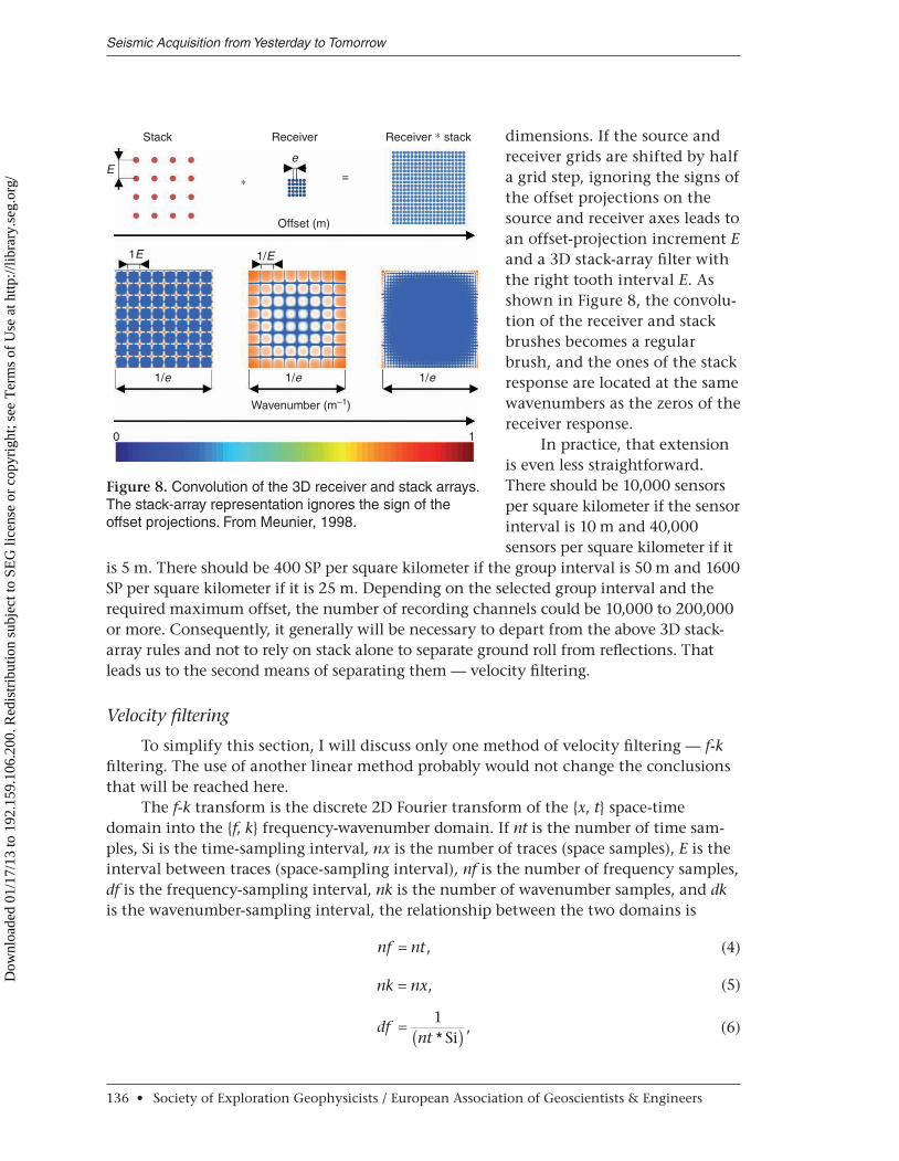
dimensions. If the source and receiver grids are shifted by half a grid step, ignoring the signs of the offset projections on the source and receiver axes leads to an offset-projection increment E and a 3D stack-array filter with the right tooth interval E. As shown in Figure 8, the convolu-tion of the receiver and stack brushes becomes a regular brush, and the ones of the stack response are located at the same wavenumbers as the zeros of the receiver response.

In practice, that extension is even less straightforward. There should be 10,000 sensors per square kilometer if the sensor interval is 10 m and 40,000 sensors per square kilometer if it

is 5 m. There should be 400 SP per square kilometer if the group interval is 50 m and 1600 SP per square kilometer if it is 25 m. Depending on the selected group interval and the required maximum offset, the number of recording channels could be 10,000 to 200,000 or more. Consequently, it generally will be necessary to depart from the above 3D stack-array rules and not to rely on stack alone to separate ground roll from reflections. That leads us to the second means of separating them — velocity filtering.

Velocity filtering

To simplify this section, I will discuss only one method of velocity filtering — f-k filtering. The use of another linear method probably would not change the conclusions that will be reached here.

The f-k transform is the discrete 2D Fourier transform of the {x, t} space-time domain into the {f, k} frequency-wavenumber domain. If nt is the number of time sam-ples, Si is the time-sampling interval, nx is the number of traces (space samples), E is the interval between traces (space-sampling interval), nf is the number of frequency samples, df is the frequency-sampling interval, nk is the number of wavenumber samples, and dk is the wavenumber-sampling interval, the relationship between the two domains is

nf nt= , (4)

nk nx= , (5)

dfnt *

,= ( )1

Si (6)



Stack

0 1

E

1E 1/E

1/e 1/e 1/e

e

Receiver

Offset (m)

Wavenumber (m–1)

=

Receiver ∗ stack

∗

Figure 8. Convolution of the 3D receiver and stack arrays. The stack-array representation ignores the sign of the offset projections. From Meunier, 1998.

Dow

nloa

ded

01/1

7/13

to 1

92.1

59.1

06.2

00. R

edis

trib

utio

n su

bjec

t to

SEG

lice

nse

or c

opyr

ight

; see

Ter

ms

of U

se a

t http

://lib

rary

.seg

.org

/

and

dknx E

*

.= ( )1

(7)

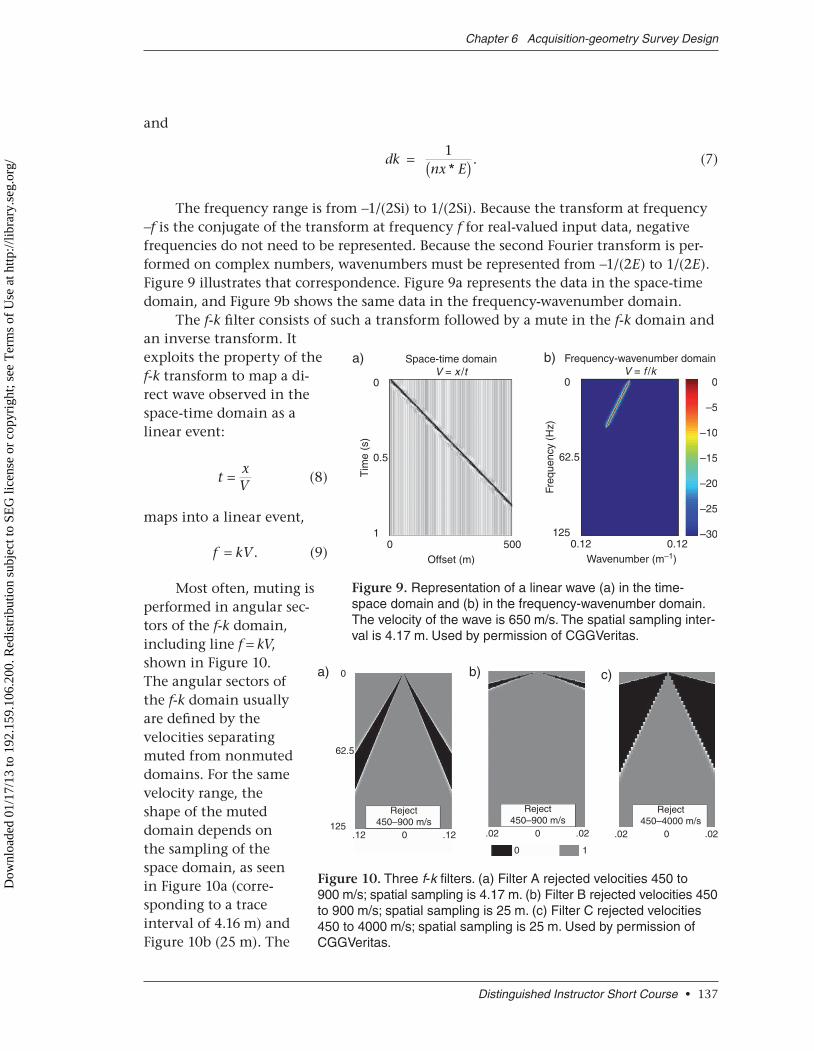
The frequency range is from −1/(2Si) to 1/(2Si). Because the transform at frequency −f is the conjugate of the transform at frequency f for real-valued input data, negative frequencies do not need to be represented. Because the second Fourier transform is per-formed on complex numbers, wavenumbers must be represented from −1/(2E) to 1/(2E). Figure 9 illustrates that correspondence. Figure 9a represents the data in the space-time domain, and Figure 9b shows the same data in the frequency-wavenumber domain.

The f-k filter consists of such a transform followed by a mute in the f-k domain and an inverse transform. It exploits the property of the f-k transform to map a di-rect wave observed in the space-time domain as a linear event:

t

xV

=

(8)

maps into a linear event,

f kV= . (9)

Most often, muting is performed in angular sec-tors of the f-k domain, including line f = kV, shown in Figure 10. The angular sectors of the f-k domain usually are defined by the velocities separating muted from nonmuted domains. For the same velocity range, the shape of the muted domain depends on the sampling of the space domain, as seen in Figure 10a (corre-sponding to a trace interval of 4.16 m) and Figure 10b (25 m). The



Tim

e (s

)

0.5

10 500

Offset (m)

Space-time domainV = x /t

0

a)

Freq

uenc

y (H

z)0.12 0.12

Wavenumber (m–1)

Frequency-wavenumber domainV = f /k

b)

62.5

125

0 0

–30

–25

–20

–15

–10

–5

Figure 9. Representation of a linear wave (a) in the time-space domain and (b) in the frequency-wavenumber domain. The velocity of the wave is 650 m/s. The spatial sampling inter-val is 4.17 m. Used by permission of CGGVeritas.

0 1

b)

Reject450–900 m/s

.02 0 .02

c)

Reject450–4000 m/s

0 .02.02

0a)

62.5

125.12

Reject450–900 m/s

.120

Figure 10. Three f-k filters. (a) Filter A rejected velocities 450 to 900 m/s; spatial sampling is 4.17 m. (b) Filter B rejected velocities 450 to 900 m/s; spatial sampling is 25 m. (c) Filter C rejected velocities 450 to 4000 m/s; spatial sampling is 25 m. Used by permission of CGGVeritas.

Dow

nloa

ded

01/1

7/13

to 1

92.1

59.1

06.2

00. R

edis

trib

utio

n su

bjec

t to

SEG

lice

nse

or c

opyr

ight

; see

Ter

ms

of U

se a

t http

://lib

rary

.seg

.org

/

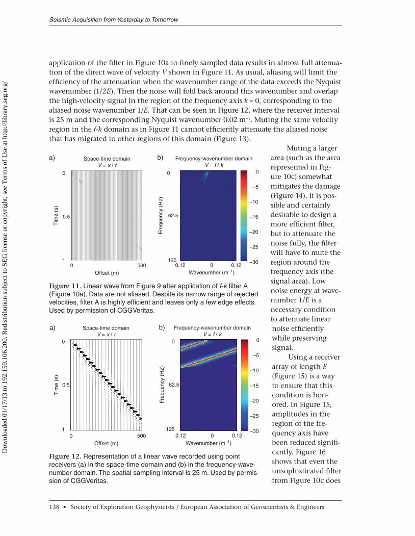
application of the filter in Figure 10a to finely sampled data results in almost full attenua-tion of the direct wave of velocity V shown in Figure 11. As usual, aliasing will limit the efficiency of the attenuation when the wavenumber range of the data exceeds the Nyquist wavenumber (1/2E). Then the noise will fold back around this wavenumber and overlap the high-velocity signal in the region of the frequency axis k = 0, corresponding to the aliased noise wavenumber 1/E. That can be seen in Figure 12, where the receiver interval is 25 m and the corresponding Nyquist wavenumber 0.02 m−1. Muting the same velocity region in the f-k domain as in Figure 11 cannot efficiently attenuate the aliased noise that has migrated to other regions of this domain (Figure 13).

Muting a larger area (such as the area represented in Fig-ure 10c) somewhat mitigates the damage (Figure 14). It is pos-sible and certainly desirable to design a more efficient filter, but to attenuate the noise fully, the filter will have to mute the region around the frequency axis (the signal area). Low noise energy at wave-number 1/E is a necessary condition to attenuate linear noise efficiently while preserving signal.

Using a receiver array of length E (Figure 15) is a way to ensure that this condition is hon-ored. In Figure 15, amplitudes in the region of the fre-quency axis have been reduced signifi-cantly. Figure 16 shows that even the unsophisticated filter from Figure 10c does



01

0.5

Tim

e (s

)

0

a)

500

Offset (m)

Space-time domainV = x / t

Freq

uenc

y (H

z)b)

–15

–20

–25

–30

0

–5

–10

125

62.5

0

0.12 0.120

Wavenumber (m–1)

Frequency-wavenumber domainV = f / k

Figure 11. Linear wave from Figure 9 after application of f-k filter A (Figure 10a). Data are not aliased. Despite its narrow range of rejected velocities, filter A is highly efficient and leaves only a few edge effects. Used by permission of CGGVeritas.

01

0.5

Tim

e (s

)

0

a)

500Offset (m)


Freq

uenc

y (H

z)

b)

–15

–20

–25

–30

0

–5

–10

125

62.5

0

0.12 0.120Wavenumber (m–1)


Figure 12. Representation of a linear wave recorded using point receivers (a) in the space-time domain and (b) in the frequency-wave-number domain. The spatial sampling interval is 25 m. Used by permis-sion of CGGVeritas.

Dow

nloa

ded

01/1

7/13

to 1

92.1

59.1

06.2

00. R

edis

trib

utio

n su

bjec

t to

SEG

lice

nse

or c

opyr

ight

; see

Ter

ms

of U

se a

t http

://lib

rary

.seg

.org

/

a good job of reducing all noise. The conclusion of this exercise could be that to allow optimal applica-tion of velocity filtering to an SP gather, the receiver-array length should equal the group interval. That recommendation is very similar to one of the stack-array recommendations. I shall not redo on cross-spread gathers the exercise conducted on SP gathers. Smith (1997) does that and shows that the conclusion derived above on SP gath-ers can be extrapolated in three dimensions to cross-spread gathers.

Smith (1997) develops the following rule: To allow optimal 3D velocity filter-ing of a cross-spread gather, the receiver-array length should equal the receiver interval, and the source-array length should equal the source interval. A vali-dation of that rule is shown in Figure 17, which repre-sents two receiver lines of the same cross-spread gather in three situations: (1) field filtering only (lin-ear arrays) in Figure 17a, (2) digital filtering only (ap-plied to point-source and point-receiver data) in Figure 17b, and (3) combined field and digital filtering in Figure 17c. The advantage of combining field arrays with velocity filter-ing is obvious. In this particular case, the field arrays are linear arrays along the source and receiver lines (as recommended by Smith [1997]). It must be noted that other solutions exist. The actual condition is that the convolution of the source by the receiver array be a 2D array of size equal to the source and receiver intervals. In particular, a point source associated with a square receiver array (or vice versa) will provide the same result, as can be appreciated from Figure 18.



01

0.5

Tim

e (s

)

0

a)

500Offset (m)


Freq

uenc

y (H

z)

b)

–15

–20

–25

–30

0

–5

–10

125

62.5

0



Figure 13. Linear wave shown in Figure 12 after application of f-k filter B (Figure 10b). Data are aliased. The reduced range of rejected velocities of filter B cannot attenuate aliased noise. Used by permission of CGGVeritas.

01

0.5

Tim

e (s

)

0

a)

500Offset (m)


Freq

uenc

y (H

z)

b)

–15

–20

–25

–30

0

–5

–10

125

62.5

0



Figure 14. Linear wave shown in Figure 12 recorded using point receivers (a) in the time-space domain and (b) in the fre-quency-wavenumber domain after application of f-k filter C (Figure 10c). The wider rejected range of velocity of filter C enables partial attenuation of the aliased noise but leaves the part of the noise that overlaps the signal area. Used by permis-sion of CGGVeritas.

Dow

nloa

ded

01/1

7/13

to 1

92.1

59.1

06.2

00. R

edis

trib

utio

n su

bjec

t to

SEG

lice

nse

or c

opyr

ight

; see

Ter

ms

of U

se a

t http

://lib

rary

.seg

.org

/

At this point, the following three rules have been established:

1) The critical interval for noise attenuation is the sensor interval (not the group interval). It should be shorter than 80% of the shortest noise wavelength.

2) In three dimensions, it generally will be necessary to combine field-array filtering with noise processing.

3) A condition for a harmonious combination of field and processing filters is that the array size be the same as the group intervals.

As in the 2D case, an alternative solution is not to use field arrays and to record signal received by each individual geophone separately. As in the 2D case, that solution will provide more flexibility and more efficiency in the separation of signal and noise. It also will reduce problems associated with arrays such as intra-array statics and residual move-out. However, keep in mind that not using arrays does not change the basic re-quirement of adequately sampling the noise. Conse-quently, to offer an indis-putable advantage over an acquisition using an n × n geophone array, the number of channels of a single-sensor acquisi-tion should be multiplied by n2.

Note that the above rules were obtained by using synthetic data. On real data, there are two major differences: (1) Sur-face waves do not behave smoothly. Their velocity and amplitude vary from place to place. (2) More-



01

0.5

Tim

e (s

)

0

a)

500Offset (m)


Freq

uenc

y (H

z)b)

–15

–20

–25

–30

0

–5

–10

125

62.5

0



Figure 15. Representation of a linear wave recorded using a 25-m receiver (a) in the space-time domain and (b) in the fre-quency-wavenumber domain. The spatial sampling interval is 25 m. Noise is attenuated in the wavenumber range, which folds back onto the zero wavenumber after aliasing. Used by permission of CGGVeritas.

01

0.5

Tim

e (s

)

0

a)

500Offset (m)


Freq

uenc

y (H

z)

b)

–15

–20

–25

–30

0

–5

–10

125

62.5

0



Figure 16. Linear wave in Figure 15 recorded (a) in the space-time domain and (b) in the frequency-wavenumber domain after application of f-k filter C (Figure 10c). The combination of linear arrays and wide-reject f-k filter results in an efficient attenuation of noise. Used by permission of CGGVeritas.

Dow

nloa

ded

01/1

7/13

to 1

92.1

59.1

06.2

00. R

edis

trib

utio

n su

bjec

t to

SEG

lice

nse

or c

opyr

ight

; see

Ter

ms

of U

se a

t http

://lib

rary

.seg

.org

/

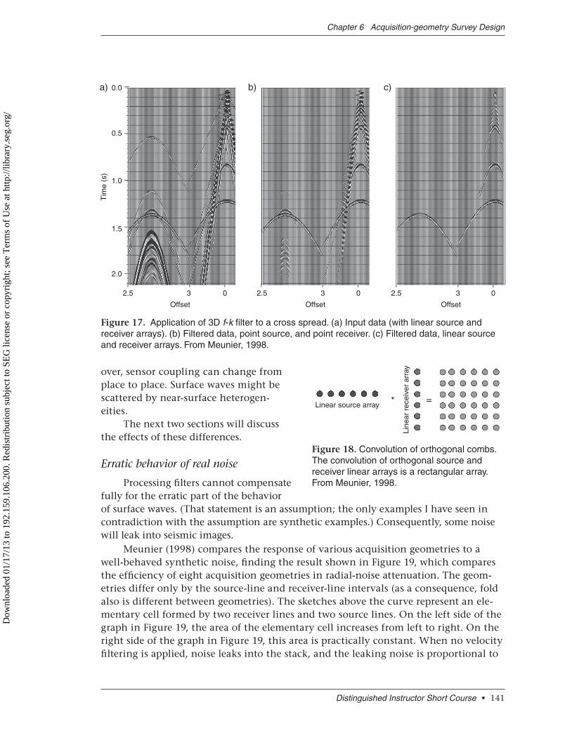
over, sensor coupling can change from place to place. Surface waves might be scattered by near-surface heterogen-eities.

The next two sections will discuss the effects of these differences.

Erratic behavior of real noise

Processing filters cannot compensate fully for the erratic part of the behavior of surface waves. (That statement is an assumption; the only examples I have seen in contradiction with the assumption are synthetic examples.) Consequently, some noise will leak into seismic images.

Meunier (1998) compares the response of various acquisition geometries to a well-behaved synthetic noise, finding the result shown in Figure 19, which compares the efficiency of eight acquisition geometries in radial-noise attenuation. The geom-etries differ only by the source-line and receiver-line intervals (as a consequence, fold also is different between geometries). The sketches above the curve represent an ele-mentary cell formed by two receiver lines and two source lines. On the left side of the graph in Figure 19, the area of the elementary cell increases from left to right. On the right side of the graph in Figure 19, this area is practically constant. When no velocity filtering is applied, noise leaks into the stack, and the leaking noise is proportional to



2.5

2.0

1.5

1.0

Tim

e (s

)

0.5

0.0a) b) c)

3

Offset

0 2.5 3 0 2.5 3 0

Offset Offset

Figure 17. Application of 3D f-k filter to a cross spread. (a) Input data (with linear source and receiver arrays). (b) Filtered data, point source, and point receiver. (c) Filtered data, linear source and receiver arrays. From Meunier, 1998.

Linear source array * =Li

near

rec

eive

r ar

ray

Figure 18. Convolution of orthogonal combs. The convolution of orthogonal source and receiver linear arrays is a rectangular array. From Meunier, 1998.

Dow

nloa

ded

01/1

7/13

to 1

92.1

59.1

06.2

00. R

edis

trib

utio

n su

bjec

t to

SEG

lice

nse

or c

opyr

ight

; see

Ter

ms

of U

se a

t http

://lib

rary

.seg

.org

/

the cell area. When velocity filtering is applied, the noise is virtually canceled, and the signal-to-noise ratio (S/N) no longer depends on line intervals.

The extrapolation from synthetic to real data turns out to be wrong because the implicit assumption that erratic behavior can be pro-cessed adequately is not true. Bianchi et al. (2008) com-pare real geometries; they explain and correct the con-clusions from Meunier (1998). The demonstration in Bianchi et al. (2008) starts with the 3D stack response. As defined in the stack-array section above, it is the 2D kx-ky transform of the 3D stack-array filter.

Such a stack response is represented in Figure 20. The signal area is shown by the red dot in the center (ampli-tude = 1) at kx = ky = 0. The other red dots correspond to wavenumbers vulnerable to noise leakage. Those peaks are the weak points of the stack response and are located at wavenumbers multiple of 1/2SLI and 1/2RLI. Chances of noise leakage are proportional to the density of the peaks in the stack response, and the response is proportional to the area between two source

lines and two receiver lines. Noise will leak through the stack in proportion to the area between two source and two receiver lines.

That is illustrated by the real-data example shown in Figure 21a through 21c, which represents slices of three migrated data volumes obtained with three acquisition



4

Dec

ibal

s

51015202530

300

300

200Source-line

interval

200

400

200

400

400 Receiver-line

interval

20040

0

600

600

300

300

150

600

9 16 36 8 9 8 9 Cell area(× 10,000 m2)

Linear arraysNo filter

Linear arraysfkxky filter

Figure 19. Signal-to-noise ratio estimated on CMP stack obtained with and without 3D f-k filter from eight acquisition geometries differing in source- and receiver-line intervals. From Meunier, 1998.

12RLI

Potential

Signal

noise

kx

leaksthroughthe stack

12SLI

12ymax

ky

12xmax

Figure 20. Stack response associated with orthogonal shooting with line intervals RLI and SLI and maximum inline and crossline distances xmax and ymax, respectively. From Bianchi et al., 2008.

Dow

nloa

ded

01/1

7/13

to 1

92.1

59.1

06.2

00. R

edis

trib

utio

n su

bjec

t to

SEG

lice

nse

or c

opyr

ight

; see

Ter

ms

of U

se a

t http

://lib

rary

.seg

.org

/

geometries differing essentially in source- and receiver-line intervals. The average kx-ky amplitude spectrum of several time slices is shown below each slice. The noise decreases from Figure 21a to 21c in the same proportion as the decrease in area between two source lines and two receiver lines and the decrease in density of white dots in the amplitude spectra. Those dots are found at the locations predicted by the stack response of the corresponding geometries. The receiver array was a single line of 12 receivers over 50 m along the receiver-line direction in all three cases.

It is interesting to note another dif ference among these geometries. Geometries of Figure 21a and 21b were recorded with a source interval of 25 m and an array of three vibrators over 25 m. The geometry in Figure 21c was recorded with a single vibrator with a 25-m source interval. Therefore, it presents less aliasing protection along the source-line dir ection. The effect of this reduced aliasing protection cannot be seen on the migrated data, perhaps because the effect is much lower than the line-interval footprint. I shall come back to this remark in the paragraph on high fold and aliasing.

At this point, it is possible to take into account the true behavior of the noise field and add a rule to those derived from synthetic data: Source- and receiver-line



0.01

a) b) c)

300

1.04 1.00 1.04 1.00 1.04 1.00

400

0.008

0.006

0.004

0.002

0

0.002

–0.004

–0.006

–0.008

–0.01–0.01 –0.008 –0.006 –0.004 –0.002 0 0.002 0.004 0.006 0.008 0.0

0.01

300

200

0.008

0.006

0.004

0.002

0

0.002

–0.004

–0.006

–0.008

–0.01–0.01 –0.008 –0.006 –0.004 –0.002 0 0.002 0.004 0.006 0.008 0.0

0.01

150

200

0.008

0.006

0.004

0.002

0

–0.002

–0.004

–0.006

–0.008

–0.01–0.01 –0.008 –0.006 –0.004 –0.002 0 0.002 0.004 0.006 0.008 0.0

Figure 21. Effect of source- and receiver-line intervals. Top images are time slices of migrated data volume, obtained with three acquisition geometries differing in source- (blue) and receiver-line (red) intervals, as indicated in the gray rectangles and in the source configuration: three vibrators with source interval 25 m on the (a) left and (b) center slices, and (c) one vibrator with source inter-val 25 m on the right. Bottom images represent average kx-ky amplitude spectrum of time slices. The noise decreases from left to right as the area decreases between two source lines and two receiver lines and as the density of white dots in the amplitude spectra decreases. From Bianchi et al., 2008.

Dow

nloa

ded

01/1

7/13

to 1

92.1

59.1

06.2

00. R

edis

trib

utio

n su

bjec

t to

SEG

lice

nse

or c

opyr

ight

; see

Ter

ms

of U

se a

t http

://lib

rary

.seg

.org

/

intervals eventually control residual noise attenuation by the 3D stack. Note that for a given receiver-patch area, stacking fold is inversely proportional to the area be-tween two source and two receiver lines. Am I saying that a higher stacking fold results in better noise reduction? Yes, but I am adding the information that noise is attenuated in proportion to the fold and not in proportion to the square root of the fold. Stacking is known to attenuate “random” noise in proportion to the square root of the fold. For a given receiver-patch area, stacking attenuates organized noise in direct proportion to the fold. Thus, this is not such a naive rule after all. It implies that line intervals, not fold (which is related to them), are the primary parameters to be considered.

Scattered noise

One of the most erratic behaviors of surface waves is their scattering by surface heterogeneities. The importance of that phenomenon makes it deserving of a special section. Meunier (1999) notes that in the cross-spread domain, scattered noise is found on diamondlike surfaces (sections of rounded pyramids) whose shape depends on the location of the diffracting point, and in the source and receiver domains, scattered noise is found on circles (sections of cones) whose shape is independent of the diffracting-point location. That is seen in Figure 22, which represents 2 × 2 simu-lated time slices in the same model observed in those two domains. The model con-sists of radial noise (the larger circle on each slice) and reemitted noise by three

surface points (the smaller circles or diamonds).

Figure 23 represents three frequency slices of the 3D f-k transforms of the total noise. In the SP domain (Fig-ure 23a), radial and scattered noises are found on the same cone (circles in the left and center slices corresponding with frequencies where noise is not aliased). The complex shape depicted in the right slice corresponds with a fre-quency at which noise is aliased. In the cross-spread domain (Figure 23b), the scattered field is scattered over the f-k volume, particu-larly in the signal area in the center of the frequency slices. Figure 23b corresponds to a frequency at which that noise is aliased. Meunier (1999)



x (m)

Cross spread

3D shotpoint

t = 3st = 2s

y (m

)

Figure 22. Time slices of a radial noise and three scattered noises. In the SP domain, the scattered noises are found on cones tangent to the radial cone. In the cross-spread domain, the radial noise is found on the cone, but the scattered noise is found on diamondlike surfaces. From Meunier, 1999.

Dow

nloa

ded

01/1

7/13

to 1

92.1

59.1

06.2

00. R

edis

trib

utio

n su

bjec

t to

SEG

lice

nse

or c

opyr

ight

; see

Ter

ms

of U

se a

t http

://lib

rary

.seg

.org

/

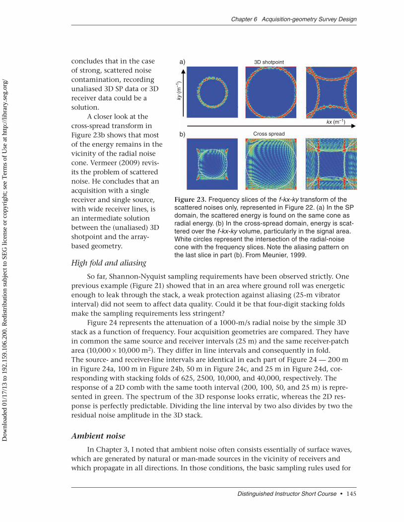
concludes that in the case of strong, scattered noise contamination, recording unaliased 3D SP data or 3D receiver data could be a solution.

A closer look at the cross-spread transform in Figure 23b shows that most of the energy remains in the vicinity of the radial noise cone. Vermeer (2009) revis-its the problem of scattered noise. He concludes that an acquisition with a single receiver and single source, with wide receiver lines, is an intermediate solution between the (unaliased) 3D shotpoint and the array-based geometry.

High fold and aliasing

So far, Shannon-Nyquist sampling requirements have been observed strictly. One previous example (Figure 21) showed that in an area where ground roll was energetic enough to leak through the stack, a weak protection against aliasing (25-m vibrator interval) did not seem to affect data quality. Could it be that four-digit stacking folds make the sampling requirements less stringent?

Figure 24 represents the attenuation of a 1000-m/s radial noise by the simple 3D stack as a function of frequency. Four acquisition geometries are compared. They have in common the same source and receiver intervals (25 m) and the same receiver-patch area (10,000 × 10,000 m2). They differ in line intervals and consequently in fold. The source- and receiver-line intervals are identical in each part of Figure 24 — 200 m in Figure 24a, 100 m in Figure 24b, 50 m in Figure 24c, and 25 m in Figure 24d, cor-responding with stacking folds of 625, 2500, 10,000, and 40,000, respectively. The response of a 2D comb with the same tooth interval (200, 100, 50, and 25 m) is repre-sented in green. The spectrum of the 3D response looks erratic, whereas the 2D res-ponse is perfectly predictable. Dividing the line interval by two also divides by two the residual noise amplitude in the 3D stack.

Ambient noise

In Chapter 3, I noted that ambient noise often consists essentially of surface waves, which are generated by natural or man-made sources in the vicinity of receivers and which propagate in all directions. In those conditions, the basic sampling rules used for



3D shotpointa)

b)

ky (

m–1

)

kx (m–1)

Cross spread

Figure 23. Frequency slices of the f-kx-ky transform of the scattered noises only, represented in Figure 22. (a) In the SP domain, the scattered energy is found on the same cone as radial energy. (b) In the cross-spread domain, energy is scat-tered over the f-kx-ky volume, particularly in the signal area. White circles represent the intersection of the radial-noise cone with the frequency slices. Note the aliasing pattern on the last slice in part (b). From Meunier, 1999.

Dow

nloa

ded

01/1

7/13

to 1

92.1

59.1

06.2

00. R

edis

trib

utio

n su

bjec

t to

SEG

lice

nse

or c

opyr

ight

; see

Ter

ms

of U

se a

t http

://lib

rary

.seg

.org

/

source-generated noise also apply for ambient noise. However, there is a major difference. Organization of source-generated noise, direct or scat-tered, is found in all possible gathers (common source, common receiver, common offset, cross spread, and CMP). Ambient noise is organized only in SP gathers. In those gathers, ambient noise associated with any surface source will be found in the f-k domain on noise cones similar to source-generated radial and scattered noises.

To take advantage of that prop-erty, velocity filtering should be

applied to SP gathers, which therefore should be unaliased in both directions. That is a very heavy constraint. However, in some geometries such as WesternGeco’s Q-Land fat-line geometry (Figure 25), SP gathers present some limited extension of unaliased areas and could benefit partially from that property. Generally, the property will con-cern only the receiver array. If the sensor interval is shorter than half the shortest ground-roll wavelength, the receiver array can reduce ambient noise slightly more than it would reduce random noise.



Figure 25. Fat-line acquisition geometry providing some limited unaliased areas. The resulting width of the receiver lines provides protection against transverse noise similar to the protection provided by an array of identical width. Used by permission of CGGVeritas.

Line interval 200 m0

a)

–10

–20

–30

–400 10 20

Frequency (Hz)30 40

Fold 625


b)

Dec

ibel

s

–10

–20

–30

–400 10 20

Frequency (Hz)30 40

Fold 2500

2D 3D


c)

–10

–20

–30

–400 10 20

Frequency (Hz)

30 40

Fold 10,000


d)

Dec

ibel

s

–10

–20

–30

–400 10 20

Frequency (Hz)

30 40

Fold 40,000

Figure 24. Ground-roll attenuation by 3D stack. When the line interval decreases, noise attenuation in-creases in two ways. First, the minimum attenuation increases (from 8 dB for an inter-val of 200 m to 20 dB for an interval of 25 m). Second, the number of unattenuated frequen-cies decreases (only 20, 28, and 40 Hz in this example). Used by permission of CGG-Veritas.

Dow

nloa

ded

01/1

7/13

to 1

92.1

59.1

06.2

00. R

edis

trib

utio

n su

bjec

t to

SEG

lice

nse

or c

opyr

ight

; see

Ter

ms

of U

se a

t http

://lib

rary

.seg

.org

/

Conclusions on noise constraints

We can draw several conclusions regarding noise constraints:

The critical interval for noise attenuation is the sensor interval, which should be • shorter than 80% of the shortest noise wavelength. That interval is adequate for both source- generated and ambient noises. This rule holds for single-sensor acquisition.In three dimensions, except for very high folds, the stack response does not attenu-• ate noise adequately. Generally, it will be necessary to combine field-array filtering with noise processing.A condition for harmonious combination is that the array size must be the same as • the group interval. In that sense, a single-sensor acquisition is always harmonious.Residual noise in the seismic image is proportional to the product of source- and • receiver-line intervals.Residual ambient noise in the seismic image is inversely proportional to the square • root of the total receiver area. That result was obtained in Chapter 4.

Signal constraints

As noted in the introduction to this chapter, two other types of limitations besides noise affect data quality — imaging limitations and human error. Imaging limitations — the finite size of the wavefield observation surface and the sampling of the surface — are discussed in this section. I will present an imaging exercise to highlight the relationship between acquisition and imaging. After a preliminary comment on sampling limitations, I will start the exercise in two dimensions for the sake of simplicity before looking at the more general 3D case. The same exercise also will be used to discuss survey-design strategy in case of obstacles.

Preliminary remark on sampling limitations

The shortest wavelength to be imaged should be sampled at least twice, according to the Shannon-Nyquist theorem. Some imaging procedures do not honor that con-straint strictly. It must be understood that the Shannon-Nyquist theorem holds, and that those imaging procedures replace the missing samples using some kind of assump-tion. This is not the place to discuss those assumptions.

The migration algorithm used in the following exercise is a Kirchhoff 2D depth migration (or 3D when applicable) with no antialias filtering. The signal is a band- limited wavelet with a spectrum extending as high as 40 Hz, represented in Figure 26. In a medium of velocity 2000 m/s, its wavenumber spectrum extends as high as 0.04 m−1. The image-sampling interval is 10 m, corresponding to a Nyquist wavenumber of 0.05 m−1. For display purposes (and as a reminder that the Shannon-Nyquist theorem is true), images have been interpolated at a sampling interval of 1 m. Such an interpolation of a perfectly migrated diffracting point (see below) is presented in Figure 27. The theo-retical image is circular. The input data in Figure 27a barely honor the Shannon-Nyquist criterion. The interpolated image (Figure 27b) is indeed circular. The other assumptions are that the velocity field is perfectly known and that there is no noise in the input data.



Dow

nloa

ded

01/1

7/13

to 1

92.1

59.1

06.2

00. R

edis

trib

utio

n su

bjec

t to

SEG

lice

nse

or c

opyr

ight

; see

Ter

ms

of U

se a

t http

://lib

rary

.seg

.org

/

2D imaging exercise

If the wavefield on a continuous surface surrounding the volume to be imaged (such as a sphere) could be determined, it theoretically would be possible to obtain an optimal image. However, for the image to be optimal, a third required condition is that adequate knowledge of wave-propagation properties (essentially velocity) be available.

The following imaging exercise gives an idea of what is lost because of the two funda-mental limitations (limited extension of the observation surface and inadequate sampling of the surface). The first experiment is depicted in Figure 28a. It represents three diffracting



–80

a)

–40

0

40

80

–100 –50 0

x (m)

z (m

)

50 100

b)–80

–40

0

40

80

–100 –50 0

x (m)

z (m

)

50 100

Figure 27. Interpolation of images from a 10-m sampling interval to a 1-m sampling interval. (a) The input data barely honor the Shannon-Nyquist theorem. (b) Interpolated data. Interpolation is performed in the wavenumber domain. The curve represents the input spatial wavelet. Used by permission of CGGVeritas.

b)

1

0.8

0.6

0.4

0.2

00 0.02 0.04

Wavenumber (m–1)

0.06 0.08

0.3a)

0.25

0.2

0.15

0.1

0.05

0

–0.05

–0.1–200 –100 0

Depth (m)

Am

plitu

de

100 200

Figure 26. Signal used in the imaging exercise (a) in the depth domain and (b) in the wavenumber domain. The wavenumber spectrum extends from 0.0004 to 0.04 m−1. Used by permission of CGGVeritas.

Dow

nloa

ded

01/1

7/13

to 1

92.1

59.1

06.2

00. R

edis

trib

utio

n su

bjec

t to

SEG

lice

nse

or c

opyr

ight

; see

Ter

ms

of U

se a

t http

://lib

rary

.seg

.org

/

points, D1, D2, and D3, in a homogeneous and isotropic 2D medium with velocity 2000 m/s. A large quantity of collocated source-receiver pairs is deployed on a circle of 1-km radius. The circle constitutes the wavefield observation “surface.” Diffracting point D1 is near the center; its diffraction response is represented in Figure 28b. If D1 moved toward the center of the circle, its diffraction response would flatten progressively around the two-way traveltime along a radius of the circle. Diffraction point D2 is still inside the circle but closer to its periphery; its response shows more variations (Figure 28c). Diffraction point D3 is outside the circle; its response has slightly more variations (Figure 28d).

Figure 29 represents the migrated image of those three points. The images of D1 (Figure 29a) and D2 (Figure 29b) are nearly perfect disks. The image of D3 (Figure 29c) is distorted and is contaminated by migration noise. Two nearly linear events that form a cross superimposed on the image are related to the limitation of observation angles. Fixing that image will require much more than a sophisticated migration algorithm. It requires the collection and input of more data in the imaging process. It is also conve-nient to analyze in the kx-kz domain.

Figure 30 shows the kx-kz transforms of the data in Figure 29. The transforms of points D1 (Figure 30a) and D2 (Figure 30b) have the same circular shape. The transform



2000

a)

b)

c)

d)0

0.5

1

1.5Tim

e (s

)

2

1500

1000

500

0

0.5

1

1.5

2

–1000 –500 0 500

Source/receiverpairs

D1

D2

D3

Diffracting-point acquisition geometry

Response of diffracting point D1



x (m)

Theta (°)

z (m

)

Tim

e (s

)

0

0.5

1

1.5

2T

ime

(s)

θ

α

1000 1500

50 100 150 200 250 300 350

Theta (°)

50 100 150 200 250 300 350

Theta (°)

50 100 150 200 250 300 350

Figure 28. Observation of 2D diffracting points on a circle in a homogeneous isotropic medium of velocity 2000 m/s. (a) Experiment description. The radius of the collocated source-receiver circle is 1 km. The angle of the ray relative to the vertical downward direction is α. D1 and D2 are inside the circle; D3 is outside. (b) Seismic response of D1. (c) Seismic response of D2. (d) Seismic response of D3. Used by permission of CGGVeritas.

Dow

nloa

ded

01/1

7/13

to 1

92.1

59.1

06.2

00. R

edis

trib

utio

n su

bjec

t to

SEG

lice

nse

or c

opyr

ight

; see

Ter

ms

of U

se a

t http

://lib

rary

.seg

.org

/

of D3 (Figure 30c) is missing two symmetrical portions. Angle α (represented in Fig-ure 28) is the limit of the illumination range; it is the same angle shown on the response of point D3 in Figure 30c. The missing portions of the D3 ring in Figure 30c correspond to the missing illumination. The ring can be considered as a set of wave-number vector components of equal amplitudes (discussed later), which are parallel to the direction of propagation.

When there is no raypath in a given direction, the amplitude in that direction goes to zero. In fact, it is not necessary for the target to be seen from a full 360° angle range — 180° is sufficient. That property is connected with the symmetry seen in Figure 30 and is



1000a)

1040

1080

1120

z (m

)

z (m

)

z (m

)

1160

1200300 350 400 450 500

D1 b)1400

D2

1440

1480

1520

1560

1600700 750 800 850 900

x (m)x (m)x (m)

c) D3800

840

880

920

960

10001100 1150 1200 1250 1300

Figure 29. Migrated image of diffracting points (constant velocity). (a) Point D1, inside and close to the center of the circle. (b) Point D2, inside and close to the periphery of the circle. (c) Point D3, outside the circle. Used by permission of CGGVeritas.

–35 –30 –25 –20

Decibels

–15 –10 –5 0

–0.06

a) b) c)

–0.04

–0.02

kz (

m–1

)

0

0.02

0.04

0.06–0.06 –0.02

kx (m–1)

0.020

D1

0.06

–0.06

–0.04

–0.02

0

0.02

0.04

0.06–0.06 –0.02

kx (m–1)

0.020

D2

0.06

–0.06

–0.04

–0.02

0

0.02

0.04

0.06–0.06 –0.02

kx (m–1)

0.020

D3

0.06

α

Figure 30. The kx-kz transforms of the images in Figure 29. The transforms of (a) D1 and (b) D2 are complete rings covering the full 360° angle range. (c) The transform of D3 is an incomplete ring. Contrary to D1 and D2, D3 is not illuminated fully. Angle α, which limits the observation range in Figure 28, is the same as angle α shown in the D3 response in part (c). Used by permission of CGGVeritas.

Dow

nloa

ded

01/1

7/13

to 1

92.1

59.1

06.2

00. R

edis

trib

utio

n su

bjec

t to

SEG

lice

nse

or c

opyr

ight

; see

Ter

ms

of U

se a

t http

://lib

rary

.seg

.org

/

illustrated in Figure 31. In Figure 31a, the circle has been split into two arcs (blue and red), from which diffracting point D2 is observed over a 180° range. Imaging of point D2 is performed twice using the blue (Figure 31b) and red (Figure 31c) arcs, respectively. Images remain circular, although an artifact can be observed that corresponds to the observation limit at ± 90° from vertical. Figure 31d represents the kx-kz transform of the blue image.

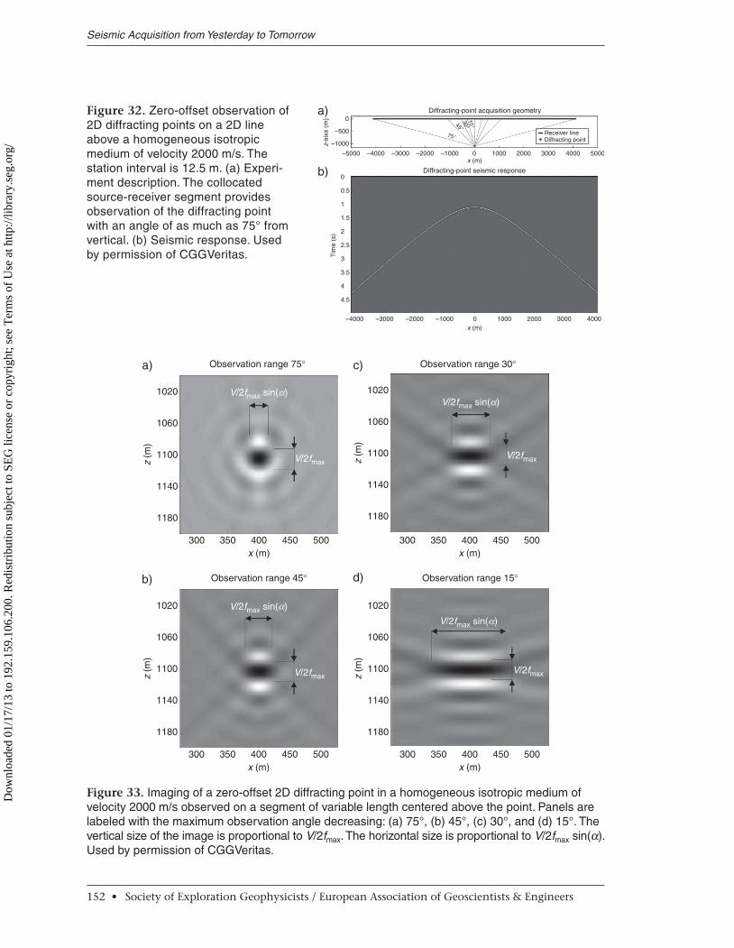
The next step is to deploy the collocated source-receiver pairs on the surface of a homogeneous and isotropic 2D medium. Figure 32 represents a corresponding 2D experiment and the modeled data. The line extent allows observation up to an angle of 75°. Figure 32a shows four observations angles along with the corresponding offset ranges; the angles are the maximum illumination angles seen in Figures 33 and 34. They progressively decrease from 75° to 15°. The largest angle (75°) corresponds to the full data set in Figure 32b. This unrealistic observation range yields an almost circular



2000

a)

1600

z (m

)

x (m)

1200

800

400

d)

–0.04

–0.02kz

(m

–1)

0

0.02

0.04

–1000 1000–500 5000

b)

1420

1460

z (m

)

1500

1540

1580

x (m)

700 900750 850800

c)

1420

1460

z (m

)

1500

1540

1580

x (m)

700 900750 850800

kx (m–1)

–0.06 0.04 0.06–0.04 –0.02 0.020

Figure 31. Imaging using a half-circle (180°). (a) The circle is split into two arcs (blue and red) that observe the diffracting point D2 over a 180° range. (b) The image obtained by using the blue arc. (c) The image obtained by using the red arc. (d) The kx-kz transform of the blue image. Its color scale goes from deep red (0 dB) to deep blue (−35 dB). Used by permission of CGGVeritas.

Dow

nloa

ded

01/1

7/13

to 1

92.1

59.1

06.2

00. R

edis

trib

utio

n su

bjec

t to

SEG

lice

nse

or c

opyr

ight

; see

Ter

ms

of U

se a

t http

://lib

rary

.seg

.org

/



Diffracting-point acquisition geometrya)

b) Diffracting-point seismic response

0

0

0.5

1

1.5

2

2.5

Tim

e (s

)

3

3.5

4

4.5

–4000 –3000 –2000 –1000 1000 2000 3000 40000x (m)

x (m)

–500

z-ai

xs (

m)

–1000

–5000 –4000 –3000 –2000 –1000 1000

75°

45°

30°15°

2000 3000 4000 50000

Receiver lineDiffracting point

Figure 32. Zero-offset observation of 2D diffracting points on a 2D line above a homogeneous isotropic medium of velocity 2000 m/s. The station interval is 12.5 m. (a) Experi-ment description. The collocated source-receiver segment provides observation of the diffracting point with an angle of as much as 75° from vertical. (b) Seismic response. Used by permission of CGGVeritas.

Observation range 75∞a)

1020

1060

z (m

)

1100

1140

1180

300 350 400 500450

V/2fmax sin(a)

V/2fmax

Observation range 45∞b)

1020

1060

z (m

)

x (m)

1100

1140

1180

300 350 400 500450

V/2fmax sin(a)

V/2fmax

x (m)

Observation range 30∞c)

1020

1060

z (m

)

x (m)

1100

1140

1180

300 350 400 500450

V/2fmax sin(a)

V/2fmax

Observation range 15∞d)

1020

1060

z (m

)

x (m)

1100

1140

1180

300 350 400 500450

V/2fmax sin(a)

V/2fmax

Figure 33. Imaging of a zero-offset 2D diffracting point in a homogeneous isotropic medium of velocity 2000 m/s observed on a segment of variable length centered above the point. Panels are labeled with the maximum observation angle decreasing: (a) 75°, (b) 45°, (c) 30°, and (d) 15°. The vertical size of the image is proportional to V/2fmax. The horizontal size is proportional to V/2fmax sin(α). Used by permission of CGGVeritas.

Dow

nloa

ded

01/1

7/13

to 1

92.1

59.1

06.2

00. R

edis

trib

utio

n su

bjec

t to

SEG

lice

nse

or c

opyr

ight

; see

Ter

ms

of U

se a

t http

://lib

rary

.seg

.org

/

image. When the range decreases toward more realistic values, the image picks up some noise and becomes progressively more elongated horizontally.

Analysis is performed best in the kx-ky domain. Figure 34 represents the kx-ky transform of the data in Figure 33. Despite some numerical complications in the region of the truncation, the truncation of the wavefield observation range is obvious. The missing parts of the ring increase steadily when the observation range decreases. Figure 35 is a close-up of Figure 34b. In Figure 35, fmax is the maximum frequency in the data (36 Hz), αmax is the maximum observation angle (45° for Figure 34b), and V is the (constant) velocity (2000 m/s). Note that although strictly speaking, the spectrum extends up to 40 Hz, fmax has been set to 36 Hz, the frequency at which the amplitude is divided by 2.

The maximum observation angles αmax indicated in Figure 33 are also the maxi-mum angles of the k(α) vector in the kx-ky domain shown in Figure 34. The image size



Observation range 75∞

75∞

a)

–0.04

–0.02

–0.06–0.04–0.02 0 0.02 0.04 0.06

kz (

m–1

)

0.02

0.04

0

kx (m–1)


45∞

b)

–0.04

–0.02

–0.06–0.04–0.02 0 0.02 0.04 0.06

kz (

m–1

)

0.02

0.04

0

kx (m–1)


30∞

c)

–0.04

–0.02

–0.06–0.04–0.02 0 0.02 0.04 0.06

kz (

m–1

)

0.02

0.04

0

kx (m–1)


15∞

d)

–0.04

–0.02

–0.06–0.04–0.02 0 0.02 0.04 0.06

kz (

m–1

)

0.02

0.04

0

kx (m–1)

Figure 34. The kx-kz transforms of the images shown in Figure 33. The maximum observation angle decreases: (a) 75°, (b) 45°, (c) 30°, and (d) 15°. The maximum angle of the k(α) vector decreases in precisely the same way. The color scale goes from deep red (0 dB) to deep blue (−35 dB). Used by permission of CGGVeritas.

Dow

nloa

ded

01/1

7/13

to 1

92.1

59.1

06.2

00. R

edis

trib

utio

n su

bjec

t to

SEG

lice

nse

or c

opyr

ight

; see

Ter

ms

of U

se a

t http

://lib

rary

.seg

.org

/

in any direction α of the space domain is inversely proportional to the maximum mod-ulus of the k(α) vector in that direction. In particular, the vertical and horizontal sizes of the image are

IszVf

IsxV

f

=

=

k

k a

2

2

max

max maxsin( )

.

(10)

Proportionality constant κ is a matter of appreciation. Isz and Isx are indicated in Figure 33 by using κ = 1.

After looking at the size of the observation surface, it remains to look at the sam-pling of the surface. Again, I shall restrict the surface to a single dimension. For this experiment, I chose a 20-m reference interval in such a way that the maximum observa-tion angle αmax verifies

sin( )

* *.max

maxa = V

f e4 ref (11)

With V = 2000 m/s, fmax = 36 Hz, and selecting the reference interval eref = 20 m, αmax = 44°.

Figure 36 shows the result of the sampling experiment. I used the same model from the segment-length experiment (velocity is 2000 m/s and point depth is 1100 m) and used eight sampling intervals of 5 to 40 m. Four sampling intervals are represented in Figure 36. The display gain is selected in such a way that the aliasing effect can be observed easily. With a 10-m interval (Figure 36a), the only observable artifacts are truncation artifacts. With a 20-m interval (Figure 36b), some noise starts to appear in the region of those artifacts. In Figure 36c and 36d, with intervals of 30 and 40 m, respectively, migration noise contaminates the image.



–0.06

–0.04

–0.02

0

kz (

m–1

)

0.02

0.04

–0.05 0 0.050.06

kx (m–1)

kmax sin(amax)

kmax = 2*fmax/V

kmin = 2*fmin/V

amax

k(amax)

Figure 35. Close-up of the 45° observation-range panel in Figure 34b. The kx-ky ring is limited by two circles with radii k f V k f Vmin min max max2 and 2= = . The nonzero parts of the ring are found between extreme observation angles −αmax and +αmax. The maximum value in the kx dimension is kmax sin(αmax). The color scale goes from deep red (0dB) to deep blue (−35dB). Used by permission of CGGVeritas.

Dow

nloa

ded

01/1

7/13

to 1

92.1

59.1

06.2

00. R

edis

trib

utio

n su

bjec

t to

SEG

lice

nse

or c

opyr

ight

; see

Ter

ms

of U

se a

t http

://lib

rary

.seg

.org

/

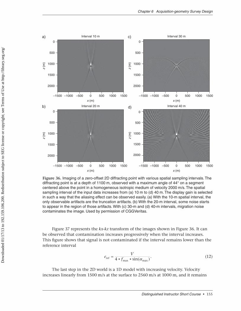
Figure 37 represents the kx-kz transform of the images shown in Figure 36. It can be observed that contamination increases progressively when the interval increases. This figure shows that signal is not contaminated if the interval remains lower than the reference interval

e

Vfref =

4 * * sin( ).

max maxa (12)

The last step in the 2D world is a 1D model with increasing velocity. Velocity increases linearly from 1500 m/s at the surface to 2560 m/s at 1000 m, and it remains



Interval 10 ma)0

500

1000

z (m

)

x (m)

1500

–1500 –1000 –500 500 1000 15000

2000

Interval 20 mb)0

500

1000

z (m

)

x (m)

1500

–1500 –1000 –500 500 1000 15000

2000

Interval 30 mc)0

500

1000

z (m

)

x (m)

1500

–1500 –1000 –500 500 1000 15000

2000

Interval 40 m

x (m)

–1500 –1000 –500 500 1000 15000

d)0

500

1000z

(m)

1500

2000

Figure 36. Imaging of a zero-offset 2D diffracting point with various spatial sampling intervals. The diffracting point is at a depth of 1100 m, observed with a maximum angle of 44° on a segment centered above the point in a homogeneous isotropic medium of velocity 2000 m/s. The spatial sampling interval of the input data increases from (a) 10 m to (d) 40 m. The display gain is selected in such a way that the aliasing effect can be observed easily. (a) With the 10-m spatial interval, the only observable artifacts are the truncation artifacts. (b) With the 20-m interval, some noise starts to appear in the region of those artifacts. With (c) 30-m and (d) 40-m intervals, migration noise contaminates the image. Used by permission of CGGVeritas.

Dow

nloa

ded

01/1

7/13

to 1

92.1

59.1

06.2

00. R

edis

trib

utio

n su

bjec

t to

SEG

lice

nse

or c

opyr

ight

; see

Ter

ms

of U

se a

t http

://lib

rary

.seg

.org

/

constant thereafter. The average velocity to 1100 m (depth of the diffracting point) is 2000 m/s, identical to the constant velocity of the previous model.

Figure 38 compares imaging in this variable-velocity model (Figure 38b and 38d) with imaging in a constant-velocity model (Figure 38a and 38c). Figure 38a and 38b illustrates the responses in the xz image space, and Figure 38c and 38d shows their respective kx-kz transforms. There are essentially two differences between the two models. First, the variable-velocity image is closer to a circle — its k transform shows a wider illumination. That phenomenon is connected with raypath bending associated



Interval 10 ma)–0.04

–0.04 –0.02 0 0.02 0.04

–0.02

0.02

0.04

0

kz (

m)

kx (m)

Interval 20 mb)–0.04

–0.04 –0.02 0 0.02 0.04

–0.02

0.02

0.04

0

kz (

m)

kx (m)

Interval 30 mc)–0.04

–0.04 –0.02 0 0.02 0.04

–0.02

0.02

0.04

0

kz (

m)

kx (m)

Interval 40 md)–0.04

–0.04 –0.02 0 0.02 0.04

–0.02

0.02

0.04

0

kz (

m)

kx (m)

Figure 37. The kx-kz transforms of the images shown in Figure 36. (a) With a 10-m sampling inter-val, the kx-kz map is not contaminated. (b) Some contamination is visible with a 20-m interval in the region of the maximum k values without affecting the signal. (c and d) With a larger interval, contamination affects lower k values outside and inside the signal area. The color scale goes from deep red (0 dB) to deep blue (−35dB). Used by permission of CGGVeritas.

Dow

nloa

ded

01/1

7/13

to 1

92.1

59.1

06.2

00. R

edis

trib

utio

n su

bjec

t to

SEG

lice

nse

or c

opyr

ight

; see

Ter

ms

of U

se a

t http

://lib

rary

.seg

.org

/

with refraction. The second difference is that the image size is larger because of the faster propagation velocity at the location of the diffracting point (2560 m/s instead of 2000 m/s.)

3D imaging exercise

Offset vector tiles (OVTs), described in Chapter 2, are singlefold 3D data subsets or pseudominimal data sets with a limited range of offsets and azimuths. They constitute an appropriate input into prestack migration. They have the property of



Image slice y = y0a)

1020

1060

x (m

)

1100

1140

1180

300 350 400

x (m)

450 500

Image slice z = z0b)

1020

1060

x (m

)

1100

1140

1180

300 350 400

x (m)

450 500

kx-ky transformd)

–0.04

–0.02kz

(m

–1)

0

0.02

0.04

–0.06 –0.04 –0.02 0 0.02 0.04 0.06

kx (m–1)

kx-kz transformc)

–0.04

–0.02

kz (

m–1

)

0

0.02

0.04

–0.06 –0.04 –0.02 0 0.02 0.04 0.06

kx (m–1)

45∞

56∞

Figure 38. Imaging comparison of two zero-offset 2D diffracting points at depth 1100 m (a and c) in a constant-velocity (2000-m/s) medium and (b and d) in a medium of increasing velocity (from 1500 m/s at the surface to 2560 m/s at 1000 m). (a and b) Center of the image in the spatial domain. (c and d) The kx-kz transforms. The same line length of 2 × 1100 m is used in both cases. It provides (c) a 45° illumination in the constant-velocity case and (d) a 56° illumination in the case of increasing velocity. The color scale for the k responses goes from deep red (0 dB) to deep blue (−35 dB). Used by permission of CGGVeritas.

Dow

nloa

ded

01/1

7/13

to 1

92.1

59.1

06.2

00. R

edis

trib

utio

n su

bjec

t to

SEG

lice

nse

or c

opyr

ight

; see

Ter

ms

of U

se a

t http

://lib

rary

.seg

.org

/

encompassing discontinuities in proportion of line intervals — many small disconti-nuities if line intervals are short and fewer, large discontinuities if line intervals are long. Consequently, prestack migration of OVTs should depend on source- and receiver-line intervals. Figure 39 represents two 3D orthogonal geometries, differing in line intervals (and consequently in fold) but covering the same area with the same source and receiver intervals (25 m) and with 160 receivers per line. Table 1 shows their parameters.

For each geometry, the survey areal extent is 4 km in x and 2 km in y. For each geom-etry, the same offset vector [x = 500 m, y = −600 m] is represented. That offset vector cor-responds to an average incidence angle of 40° for a reflector depth of 500 m; it defines the OVTs that will be constructed from the respective geometries. Figures 40 and 41 represent the data obtained from a diffracting point in the center of the source and receiver grids at



Table 1. Source and receiver parameters for geometries 1 and 2.

Parameter Geometry 1 Geometry 2

Receiver interval (m) 25 25

Receiver-line interval (m) 200 100

Number of receivers per line 160 160

Number of receiver lines 8 16

Source-point interval (m) 25 25

Source-line interval (m) 250 100

Aspect ratio 0.4 0.4

250a)

1

200

600

500 b)

2

100

100

Figure 39. Two orthogonal 3D geometries. Both have 160 stations per line, and source and receiver intervals are 25 m. (a) Geometry 1 has eight receiver lines; source-line interval SLI = 250 m and receiver-line interval RLI = 200 m. (b) Geometry 2 has 16 receiver lines; source-line interval SLI = 100 m and receiver-line interval RLI = 100 m. Blue circles represent receivers, red circles represent source points, light gray rectangles represent the receivers and sources associ-ated in offset vector tiles (OVTs), and dark gray rectangles represent the CMP coverage in each OVT. The x- and y-offsets between the centers of the receiver and source segments are identical (500 and −600 m, respectively). Used by permission of CGGVeritas.

Dow

nloa

ded

01/1

7/13

to 1

92.1

59.1

06.2

00. R

edis

trib

utio

n su

bjec

t to

SEG

lice

nse

or c

opyr

ight

; see

Ter

ms

of U

se a

t http

://lib

rary

.seg

.org

/

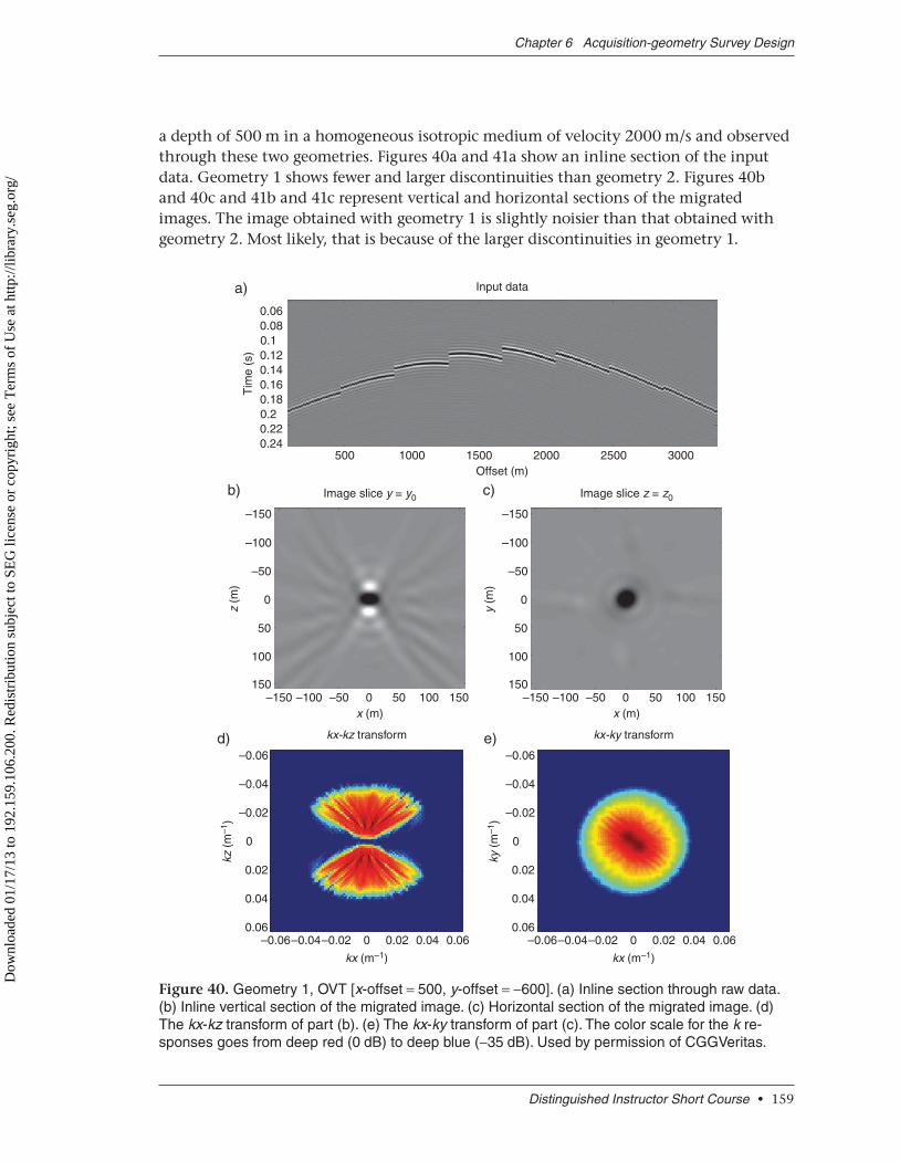
a depth of 500 m in a homogeneous isotropic medium of velocity 2000 m/s and observed through these two geometries. Figures 40a and 41a show an inline section of the input data. Geometry 1 shows fewer and larger discontinuities than geometry 2. Figures 40b and 40c and 41b and 41c represent vertical and horizontal sections of the migrated images. The image obtained with geometry 1 is slightly noisier than that obtained with geometry 2. Most likely, that is because of the larger discontinuities in geometry 1.



b) Image slice y = y0

–150

–100

–50

z (m

)

0

50

100

150–150 –100 –50 50 100 1500

x (m)

c) Image slice z = z0

–150

–100

–50

y (m

)

0

50

100

150–150 –100 –50 50 100 1500

x (m)

a) Input data

0.060.080.10.12

Tim

e (s

)

0.140.160.180.20.220.24

500 1000 1500Offset (m)

2000 30002500

d) kx-kz transform

–0.06

–0.04

–0.02

kz (

m–1

)

0

0.02

0.04

0.06–0.06–0.04–0.02 0.02 0.04 0.060

kx (m–1)

e) kx-ky transform

–0.06

–0.04

–0.02

ky (

m–1

)

0

0.02

0.04

0.06–0.06–0.04–0.02 0.02 0.04 0.060

kx (m–1)

Figure 40. Geometry 1, OVT [x-offset = 500, y-offset = −600]. (a) Inline section through raw data. (b) Inline vertical section of the migrated image. (c) Horizontal section of the migrated image. (d) The kx-kz transform of part (b). (e) The kx-ky transform of part (c). The color scale for the k re-sponses goes from deep red (0 dB) to deep blue (−35 dB). Used by permission of CGGVeritas.

Dow

nloa

ded

01/1

7/13

to 1

92.1

59.1

06.2

00. R

edis

trib

utio

n su

bjec

t to

SEG

lice

nse

or c

opyr

ight

; see

Ter

ms

of U

se a

t http

://lib

rary

.seg

.org

/

The horizontal image slices (Figures 40c and 41c) and their kx-ky transforms (Fig-ures 40e and 41e) show an elongated shape. Resolution in the direction of the average offset vector is reduced in a proportion similar to the observed reduction associated with a similar absolute offset in 2D, but it is virtually unchanged in the perpendicular direction. In other words, wide-azimuth geometry potentially provides a better resolu-tion than narrow-azimuth geometry. This comment was suggested to me by Thomas Bianchi during a discussion we had on these images.

Figure 40d and 40e and Figure 41d and 41e represent the 2D wavenumber trans-forms of Figure 40b and 40c and Figure 41b and 41c, respectively. They are very similar,



Input data

0.060.08

Tim

e (s

)

0.10.120.140.160.180.20.220.24

500 1000 1500Offset (m)

2000 2500 3000

a)

kx-kz transform–0.06

–0.06–0.04–0.02 0kx (m–1)

0.02 0.04 0.06

–0.04

kz (

m–1

) –0.02

0

0.02

0.04

0.06

d) kx-ky transform–0.06

–0.06–0.04–0.02 0kx (m–1)

0.02 0.04 0.06

–0.04

ky (

m–1

) –0.02

0

0.02

0.04

0.06

e)

Image slice y = y0 Image slice z = z0

–150

–150–100 –50 0

x (m)

50 100 150 –150–100 –50 0

x (m)

50 100 150

–100

z (m

)

–50

0

50

100

150

b)–150

–100

y (m

)

–50

0

50

100

150

c)

Figure 41. Geometry 2, OVT [x-offset = 500, y-offset = −600]. (a) Inline section through raw data. (b) Inline vertical section of the migrated image. (c) Horizontal section of the migrated image. (d) The kx-kz transform of part (b). (e) The kx-ky transform of part (c). The color scale for the k re-sponses goes from deep red (0 dB) to deep blue (−35 dB). Used by permission of CGGVeritas.

Dow

nloa

ded

01/1

7/13

to 1

92.1

59.1

06.2

00. R

edis

trib

utio

n su

bjec

t to

SEG

lice

nse

or c

opyr

ight

; see

Ter

ms

of U

se a

t http

://lib

rary

.seg

.org

/

with slightly more noise on geometry 1 again. Figure 42 has the same structure as Figures 40 and 41. It represents the response of the zero-offset OVT of geometry 1. The zero-off-set OVT is obtained by intersecting source and receiver segments. The section through the input data is now almost continuous. The most important observation for Figure 42 is the significant sharpening of both the vertical and horizontal spatial-domain images (Figure 42b and 42c), corresponding with the size increase of their wavenumber trans-



Input data

0.060.080.10.12

Tim

e (s

)

0.140.160.180.20.220.24

500 1000 1500Offset (m)

2000 2500 3000

a)

kx-kz transform

–0.06

kz (

m–1

)

kx (m–1)

–0.04

–0.02

0

0.02

0.04

0.06–0.06–0.04–0.02 0.02 0.060.040

d) kx-ky transform

–0.06

ky (

m–1

)

kx (m–1)

–0.04

–0.02

0

0.02

0.04

0.06–0.06–0.04–0.02 0.02 0.060.040

e)

Image slice y = y0

–150

z (m

)

x (m)

–100

–50

0

50

100

150–150 –100 –50 50 1501000

b) Image slice z = z0

–150

y (m

)

x (m)

–100

–50

0

50

100

150–150 –100 –50 50 1501000

c)

Figure 42. Geometry 1, OVT [0, 0]. (a) Inline section through raw data. (b) Inline vertical section of the migrated image. (c) Horizontal section of the migrated image. (d) The kx-kz transform of part (b). (e) The kx-ky transform of part (c). The color scale for the k responses goes from deep red (0 dB) to deep blue (−35 dB). Used by permission of CGGVeritas.

Dow

nloa

ded

01/1

7/13

to 1

92.1

59.1

06.2

00. R

edis

trib

utio

n su

bjec

t to

SEG

lice

nse

or c

opyr

ight

; see

Ter

ms

of U

se a

t http

://lib

rary

.seg

.org

/

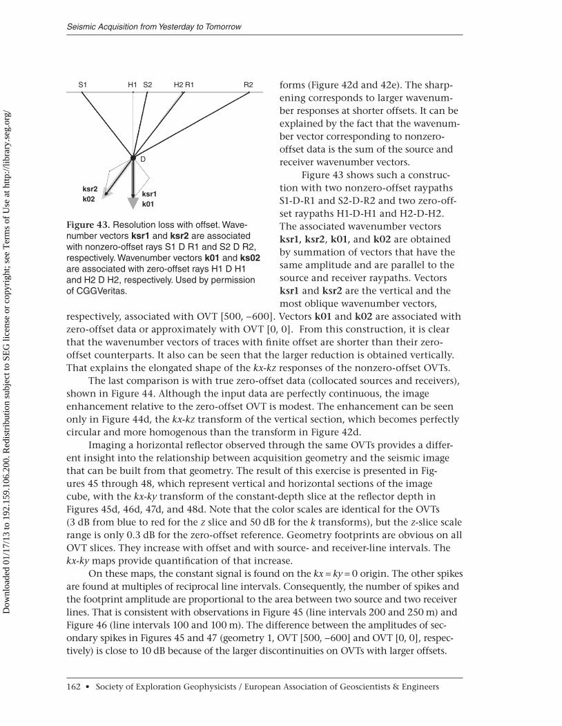
forms (Figure 42d and 42e). The sharp-ening corresponds to larger wavenum-ber responses at shorter offsets. It can be explained by the fact that the wavenum-ber vector corresponding to nonzero-offset data is the sum of the source and receiver wavenumber vectors.

Figure 43 shows such a construc-tion with two nonzero-offset raypaths S1-D-R1 and S2-D-R2 and two zero-off-set raypaths H1-D-H1 and H2-D-H2. The associated wavenumber vectors ksr1, ksr2, k01, and k02 are obtained by summation of vectors that have the same amplitude and are parallel to the source and receiver raypaths. Vectors ksr1 and ksr2 are the vertical and the most oblique wavenumber vectors,

respectively, associated with OVT [500, −600]. Vectors k01 and k02 are associated with zero-offset data or approximately with OVT [0, 0]. From this construction, it is clear that the wavenumber vectors of traces with finite offset are shorter than their zero-offset counterparts. It also can be seen that the larger reduction is obtained vertically. That explains the elongated shape of the kx-kz responses of the nonzero-offset OVTs.

The last comparison is with true zero-offset data (collocated sources and receivers), shown in Figure 44. Although the input data are perfectly continuous, the image enhancement relative to the zero-offset OVT is modest. The enhancement can be seen only in Figure 44d, the kx-kz transform of the vertical section, which becomes perfectly circular and more homogenous than the transform in Figure 42d.

Imaging a horizontal reflector observed through the same OVTs provides a differ-ent insight into the relationship between acquisition geometry and the seismic image that can be built from that geometry. The result of this exercise is presented in F ig-ures 45 through 48, which represent vertical and horizontal sections of the image cube, with the kx-ky transform of the constant-depth slice at the reflector depth in Figures 45d, 46d, 47d, and 48d. Note that the color scales are identical for the OVTs (3 dB from blue to red for the z slice and 50 dB for the k transforms), but the z-slice scale range is only 0.3 dB for the zero-offset reference. Geometry footprints are obvious on all OVT slices. They increase with offset and with source- and receiver-line intervals. The kx-ky maps provide quantification of that increase.

On these maps, the constant signal is found on the kx = ky = 0 origin. The other spikes are found at multiples of reciprocal line intervals. Consequently, the number of spikes and the footprint amplitude are proportional to the area between two source and two receiver lines. That is consistent with observations in Figure 45 (line intervals 200 and 250 m) and Figure 46 (line intervals 100 and 100 m). The difference between the amplitudes of sec-ondary spikes in Figures 45 and 47 (geometry 1, OVT [500, −600] and OVT [0, 0], respec-tively) is close to 10 dB because of the larger discontinuities on OVTs with larger offsets.



S1 H1 H2

D

ksr2k02

ksr1k01

R1 R2S2

Figure 43. Resolution loss with offset. Wave-number vectors ksr1 and ksr2 are associated with nonzero-offset rays S1 D R1 and S2 D R2, respectively. Wavenumber vectors k01 and ks02 are associated with zero-offset rays H1 D H1 and H2 D H2, respectively. Used by permission of CGGVeritas.

Dow

nloa

ded

01/1

7/13

to 1

92.1

59.1

06.2

00. R

edis

trib

utio

n su

bjec

t to

SEG

lice

nse

or c

opyr

ight

; see

Ter

ms

of U

se a

t http

://lib

rary

.seg

.org

/

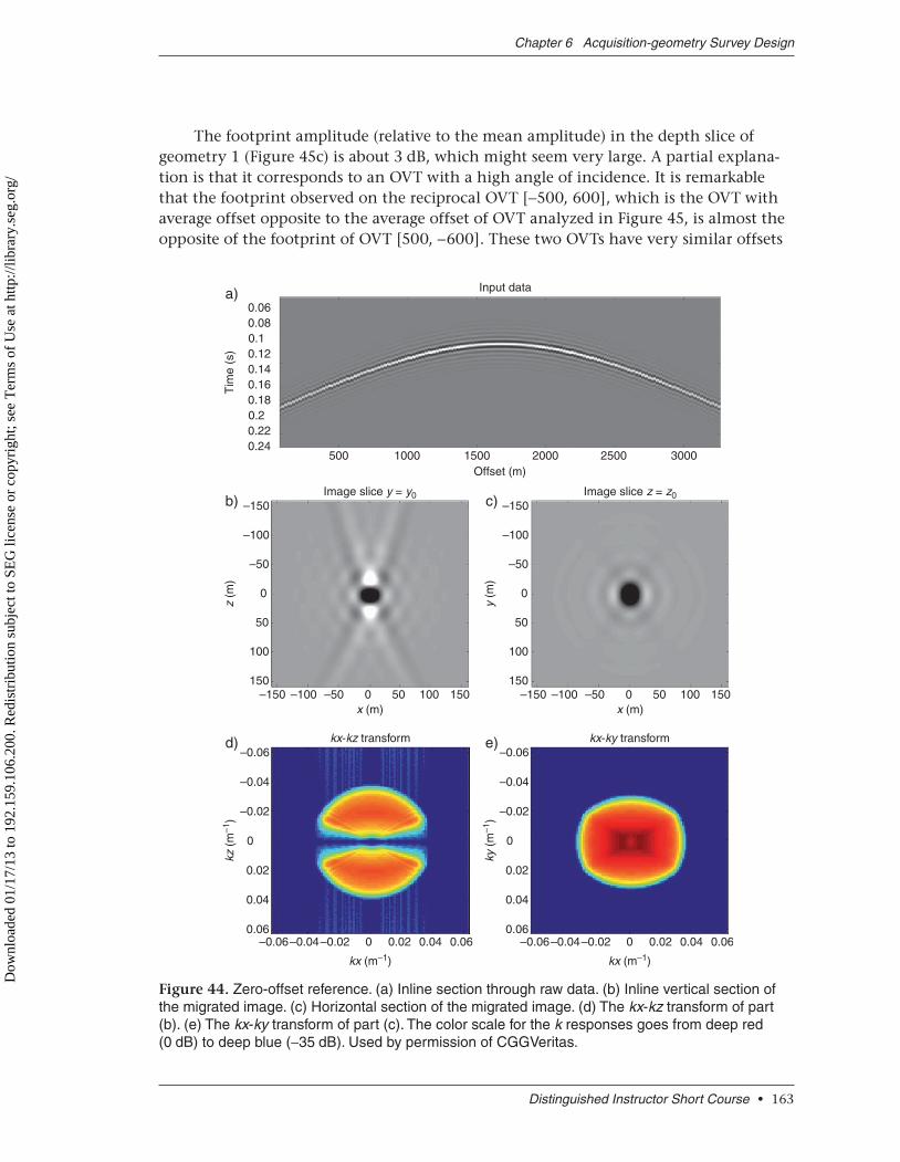
The footprint amplitude (relative to the mean amplitude) in the depth slice of geometry 1 (Figure 45c) is about 3 dB, which might seem very large. A partial explana-tion is that it corresponds to an OVT with a high angle of incidence. It is remarkable that the footprint observed on the reciprocal OVT [−500, 600], which is the OVT with average offset opposite to the average offset of OVT analyzed in Figure 45, is almost the opposite of the footprint of OVT [500, −600]. These two OVTs have very similar offsets



0.060.080.10.12

Tim

e (s

)

0.140.160.180.20.220.24

–150

–100

–50

0

50

z (m

)

100

150

–0.06

–0.04

–0.02

0

kz (

m–1

)

0.02

0.04

0.06–0.06–0.04–0.02 0

kx (m–1)

0.02 0.04 0.06

–150 –100 –50 0 50

kx-kz transform–0.06

–0.04

–0.02

0

ky (

m–1

)

0.02

0.04

0.06–0.06–0.04–0.02 0

kx (m–1)

0.02 0.04 0.06

kx-ky transform

100 150

500 1000

Image slice y = y0–150

–100

–50

0

50

y (m

)

100

150–150 –100 –50 0 50 100 150

Image slice z = z0

Offset (m)1500

Input data

2000 2500 3000

x (m) x (m)

a)

b) c)

d) e)

Figure 44. Zero-offset reference. (a) Inline section through raw data. (b) Inline vertical section of the migrated image. (c) Horizontal section of the migrated image. (d) The kx-kz transform of part (b). (e) The kx-ky transform of part (c). The color scale for the k responses goes from deep red (0 dB) to deep blue (−35 dB). Used by permission of CGGVeritas.

Dow

nloa

ded

01/1

7/13

to 1

92.1

59.1

06.2

00. R

edis

trib

utio

n su

bjec

t to

SEG

lice

nse

or c

opyr

ight

; see

Ter

ms

of U

se a

t http

://lib

rary

.seg

.org

/

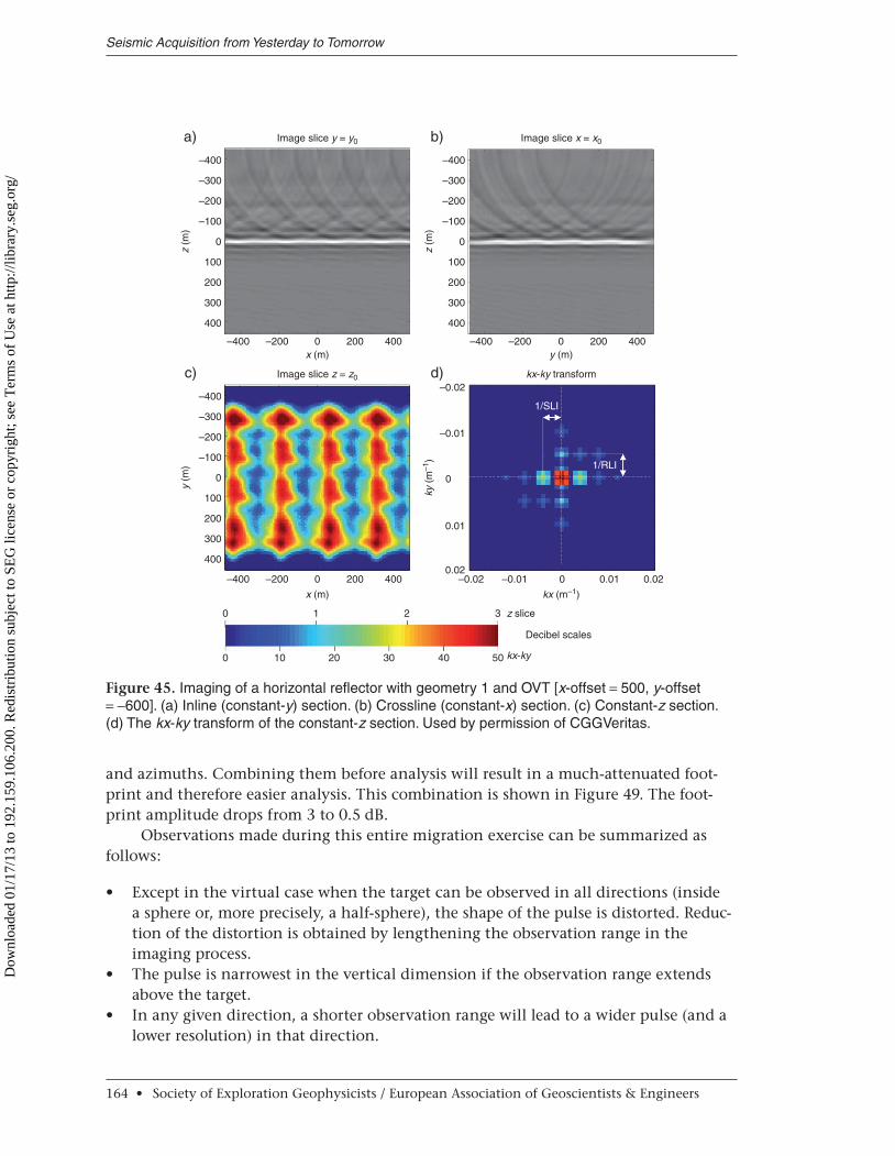
and azimuths. Combining them before analysis will result in a much-attenuated foot-print and therefore easier analysis. This combination is shown in Figure 49. The foot-print amplitude drops from 3 to 0.5 dB.

Observations made during this entire migration exercise can be summarized as follows:

Except in the virtual case when the target can be observed in all directions (inside • a sphere or, more precisely, a half-sphere), the shape of the pulse is distorted. Reduc-tion of the distortion is obtained by lengthening the observation range in the imaging process.The pulse is narrowest in the vertical dimension if the observation range extends • above the target.In any given direction, a shorter observation range will lead to a wider pulse (and a • lower resolution) in that direction.



–400

a) b)

c) d)

–300

–200

–100

0

100

z (m

)

200

300

400

–400 –200 0x (m)

Image slice y = y0

200 400

–400

–300

–200

–100

0

100

z (m

)

200

300

400

–400 –200 0y (m)

Image slice x = x0

200 400

–400

–300

–200

–100

0

100

y (m

)

200

300

400

–400 –200

0

0 10 20 30 40 50

1 2 3

Decibel scales

z slice

kx-ky

0

x (m)

Image slice z = z0

200 400

–0.02

–0.01

0

ky (

m–1

)

0.01

0.02–0.02 –0.01 0

kx (m–1)

kx-ky transform

1/SLI

1/RLI

0.01 0.02

Figure 45. Imaging of a horizontal reflector with geometry 1 and OVT [x-offset = 500, y-offset = −600]. (a) Inline (constant-y) section. (b) Crossline (constant-x) section. (c) Constant-z section. (d) The kx-ky transform of the constant-z section. Used by permission of CGGVeritas.

Dow

nloa

ded

01/1

7/13

to 1

92.1

59.1

06.2

00. R

edis

trib

utio

n su

bjec

t to

SEG

lice

nse

or c

opyr

ight

; see

Ter

ms

of U

se a

t http

://lib

rary

.seg

.org

/

Migration noise increases continuously when the spatial sampling interval increases.• For a given maximum observation angle • αmax, the signal part of the image is not

dis torted, although the sampling interval remains lower than eV

fref =4 * * sin( )max maxa

(equation 12).Zero-offset OVTs provide a close approximation of zero-offset data.• Larger line intervals lead to larger OVT discontinuities and ultimately to noisier data.• The above effect is stronger when the OVT offset increases.• Wide-azimuth geometry provides potentially higher resolution than narrow-azimuth • geometry.The sharpest images are obtained from zero-offset data.•



–400

a) b)

(c) d)

Image slice y = y0

–300

–200

–100

0

z (m

)

100

200

300

400

–400 –200 0

Image slice z = z0

x (m)200 400

–400

–300

–200

–100

0

y (m

)

ky (

m–1

)

100

200

300

400

–400

0

0 10 20 30 40 50

1 2 3 z slice

kx-ky

Decibel scales

–200 0 200 400 –0.02 –0.01 0 0.01 0.02

–400

Image slice x = x0

–300

–200

–100

0z

(m)

100

200

300

400

–0.02

–0.01

0

0.01

0.02

–400 –200

1/SLI

1/RLI

0y (m)

x (m) kx (m–1)

kx-ky transform

200 400

Figure 46. Imaging of a horizontal reflector with geometry 2 and OVT [x-offset = 500, y-offset = −600]. (a) Inline (constant-y) section. (b) Crossline (constant-x) section. (c) Constant-z section. (d) The kx-ky transform of the constant-z section. Used by permission of CGGVeritas.

Dow

nloa

ded

01/1

7/13

to 1

92.1

59.1

06.2

00. R

edis

trib

utio

n su

bjec

t to

SEG

lice

nse

or c

opyr

ight

; see

Ter

ms

of U

se a

t http

://lib

rary

.seg

.org

/

This last observation deserves some comments.

For this statement — that zero-offset data produce the best images — to be consid-• ered valid, wave-propagation characteristics should be known. How can velocity be derived from zero-offset data alone?The above exercise used a single diffracting point or a horizontal reflector in a • constant-velocity medium. In a complex environment (particularly in the case of multipaths), that analysis fails — multiple offsets are needed to construct the image. However, the zero-offset OVTs still provide the highest resolution.Finally, the cost of acquiring true zero-offset data would be very high. It would • require a dense grid of shotpoints and a dense grid of receivers. If one prediction can be made, it is that a move in the industry to acquire and use true zero-offset



–400

a) b)

c) d)

Image slice y = y0

–300

–200

–100

0

100

z (m

)

200

300

400

–400 –200 0x (m)

200 400

–400

Image slice x = x0

–300

–200

–100

0

100

z (m

)

200

300

400

–400 –200 0

1/SLI

1/RLI

y (m)200 400

–400

Image slice z = z0

–300

–200

–100

0

100

y (m

)

200

300

400

–400

0

0 10 20 30 40 50

1 2 3 z slice

kx-ky

Decibel scales

–200 0y (m)

200 400

–0.02kx-ky transform

–0.01

0

ky (

m–1

)

0.01

0.02–0.02 –0.01 0

kx (m–1)0.01 0.02

Figure 47. Imaging of a horizontal reflector with geometry 1 and OVT [0, 0]. (a) Inline (constant-y) section. (b) Crossline (constant-x) section. (c) Constant-z section. (d) The kx-ky transform of the constant-z section. Used by permission of CGGVeritas.

Dow

nloa

ded

01/1

7/13

to 1

92.1

59.1

06.2

00. R

edis

trib

utio

n su

bjec

t to

SEG

lice

nse

or c

opyr

ight

; see

Ter

ms

of U

se a

t http

://lib

rary

.seg

.org

/



–400

a) b)

c) d)

Image slice y = y0

–300

–200

–100

0

z (m

)

100

200

300

400

–400 –200 0x (m)

200 400

–400

Image slice x = x0

–300

–200

–100

0

z (m

)

100

200

300

400

–400 –200 0y (m)

200 400

–400

Image slice z = z0

–300

–200

–100

0

y (m

)

100

200

300

400

–400

0

0 10 20 30 40 50

0.1 0.2 0.3

Decibel scales

kx-ky

z slice

–200 0x (m)

200 400

–0.02kx-ky transform

–0.01

0

ky (

m–1

)

0.01

0.02–0.02 –0.01 0

kx (m–1)0.01 0.02

–500a) b) c)

–400

–300

–200

–100

100

200

300

400

500–600 –400 –200

31 32 33 34

0 200 400 600

0y (m

)

x (m)–600 –400 –200 0 200 400 600

x (m)–600 –400 –200 0 200 400 600

x (m)

Figure 49. Reciprocal offset vector tiles. (a) Geometry 1 and OVT [x-offset = 500, y-offset = −600]. Constant-depth slice. (b) Geometry 1 and OVT [x-offset = −500, y-offset = 600]. Constant depth slice (same as in Figure 43). (c) Geometry 1, (OVT [500, −600] + OVT [−500, 600])/2. Used by permission of CGGVeritas.

Figure 48. Imag-ing of a horizontal reflector. Zero-offset reference (a) Inline (con-stant-y) section. (b) Crossline (con-stant-x) section. (c) Constant-z section. (d) The kx-ky transform of the constant-z section. Used by permission of CGGVeritas.

Dow

nloa

ded

01/1

7/13

to 1

92.1

59.1

06.2

00. R

edis

trib

utio

n su

bjec

t to

SEG

lice

nse

or c

opyr

ight

; see

Ter

ms

of U

se a

t http

://lib

rary

.seg

.org

/

data is not likely. At least it is interesting to know that zero-offset data can be approximated by zero-offset OVTs. It is easier to take advantage of that property at sea than on land, where zero-offset OVTs often are contaminated by ground roll.

Most of the results from this exercise could have been predicted by a resolution analysis, as presented by Vermeer (2002, p. 159–174) and based on findings by Beylkin (1985). Sheriff (2006, p. 298) defines resolution as, “The ability to separate two features that are close together.” That ability is inversely proportional to the size of the pulses obtained in Figures 29 through 44. The value of the factor of proportionality (the κ factor in equation 10) depends on pulse shape and on the author. In Figure 33, the pulse widths obtained with κ = 1 extend roughly between the two zero crossings on each side of the pulse. In the absence of noise, it is very likely that actual resolution could be obtained with slightly lower values of κ. In the presence of noise, κ = 1 might be closer to the needed value.

This exercise illustrates the nature of the link between acquisition and imaging. Because the largest wavenumbers in seismic data often are noise wavenumbers, sampling requirements are dictated by noise but must not ignore signal. Source-receiver offsets and azimuths are needed primarily to analyze velocity and amplitude-variation-with-offset (AVO) and amplitude-variation-with-angle (AVA) behavior and to reduce noise (multiples, ground roll, and ambient noise). Source-receiver offsets and azimuths also are needed to resolve illumination and imaging difficulties in complex geologic environments, but they are not needed strictly for imaging simple structures.

In my view, the most important lesson here is the effect of source- and receiver-line intervals. In the section on noise constraints in this chapter, I showed that those inter-vals ultimately control noise reduction by stack. They also widely control imaging noise. Unfortunately, intervals are a major component of seismic cost, and they are the cause of conflict between economics and image quality. In that conflict, is it not remarkable that signal and noise, for once, have joined forces against financial officers? Today, the latter seem to retain some advantage, although there are signs that they are losing ground. Tomorrow, who knows if the need for better images might not swing the for-tune pendulum to the other side?

Errors: The lessons of 4D seismic surveys

Uncertainties and errors often are not discussed in the seismic industry, for several reasons. First, until the 1980s, the prevailing assumption in geophysics was that the world had only two dimensions. That certainly did not prevent some geophysicists from finding oil, but it did keep many of them away from sound scientific behavior. The nonvalidity of the 2D world assumption would hide measurement errors and imperfec-tions.

Second, onshore (and offshore to a lesser degree), variability in space and in time of the shallow layers in which seismic waves propagate results in a dispersion of phases and amplitudes of observed waves. Often, that dispersion is larger than the dispersion



Dow

nloa

ded

01/1

7/13

to 1

92.1

59.1

06.2

00. R

edis

trib

utio

n su

bjec

t to

SEG

lice

nse

or c

opyr

ight

; see

Ter

ms

of U

se a

t http

://lib

rary

.seg

.org

/

resulting from measurement errors or uncertainties, which makes the effects of measure-ment errors difficult to assess.

Finally, onshore and on the seafloor, sensor coupling with the formation is not perfect. In many cases, the relationship between ground motion and voltage measured at the geophone output is not linear over the full frequency range of interest. Error resulting from poor coupling can be orders of magnitude larger than error associated with geophone distortion or frequency dispersion.

The progression of 3D surveys has made us aware of the repeatability problem. Quality-control procedures were developed to assess positioning accuracy from the observation of refracted waves. Seismic crews working with single 3C receivers have understood the need and developed the procedures to ensure better receiver coupling. However, it was left to 4D seismic surveys to convince geophysicists that repeatability is a virtue we must cultivate.

There are two types of discrepancies in seismic acquisition. First, an experiment can be performed with parameters different than what they are supposed to be but with an accurate description of what they actually are. Sometimes these “errors” are unavoid-able because of various constraints such as safety distances around constructions. The second type of discrepancy is an unknown discrepancy. In a perfect experiment, the unknown discrepancy is the uncertainty of the measurement, which can be evaluated using statistical tools.

Reducing those discrepancies has been a constant concern of acquisition geophysi-cists. Offshore, positioning of sources and receivers is by far the most difficult parameter to control. A good example of such an effort to reduce both known and unknown posi-tioning discrepancies is given by Paulsen and Brown (Appendix E). They show how a combination of technical advances, including full-streamer acoustic positioning and automatic steering of vessel, sources, and streamers, can improve seismic repeatability.

Real experiments necessarily include human errors which can result in distortion of the statistical properties of the measure. That distortion can degrade the accuracy of the measure significantly and can jeopardize the estimation of uncertainty. Operators have set up quality-control procedures to track human errors as early as possible, either to repair them when the cost of repair (reshoot) is still acceptable or at least to describe them to mitigate the damage.

In the following, I will ignore human error and limit the discussion to three cases — an inaccessible area, a translation of source lines, and poor geophone coupling. For this study, I will use the orthogonal geometries presented in Figure 39 and the horizontal reflector at a depth of 500 m.

Inaccessible area

There are three ways to handle an inaccessible area:

1) Do not shoot the corresponding shotpoints or do not deploy the corresponding receivers.

2) Translate the line portion that cannot be deployed or shot in its theoretical place.3) Progressively bend the line(s) around the obstacle to keep the line(s) continuous.

That is the only possible solution in marine acquisition.



Dow

nloa

ded

01/1

7/13

to 1

92.1

59.1

06.2

00. R

edis

trib

utio

n su

bjec

t to

SEG

lice

nse

or c

opyr

ight

; see

Ter

ms

of U

se a

t http

://lib

rary

.seg

.org

/

Those three strategies are represented in Figure 50 for a circular no-shoot area of radius 250 m, using acquisition geometry 1 from Figure 39. Figure 51 illustrates the differ-ence between depth slices of the images of a horizontal reflector obtained in the three cases from Figure 50 and the same depth slice of the image obtained without perturba-tion. The depth of the reflector and of the slices is 500 m. The differences have been divided by the rms amplitude of the unperturbed image and are expressed in percentages. The corresponding percentage (50%) might seem quite high. Keep in mind that the OVT used has a large offset relative to the reflector depth. It also must be noted that the foot-print reduction associated with the reciprocal OVT is not obtained in this case. The advantage of inserting shotpoints as close as possible to the inaccessible area is obvious. Using continuous lines further reduces the amplitude of the perturbation at the cost of extending the size of the perturbed area.

In 4D acquisition, the effect of such an inaccessible area most often would be dev-astating. The skip strategy extended to all acquisition vintages might be a better

approach than trying to preserve the unperturbed image for the baseline survey and using either the translation or the continuous-line strategy for the repeat survey. When future obstructions are foreseen at the time a 4D baseline survey is recorded, a much better option would be to increase source (and perhaps receiver) density for the baseline in the area where obstructions are likely to be in-stalled. When the repeat survey is recorded, it will be possible to select the baseline and to repeat shotpoints closer to the inacces-sible area.



–800

z-slice skip Full translation

–1000 –500 0x (m)

500 1000

40

20

0

–20

–40

Continuous lines

–400

0

y (m

)

400

800

Figure 51. Inaccessible area. Difference between the images obtained using the three recording strategies of Figure 50 and the image obtained without perturbation. The differences are divided by the rms amplitude of the unperturbed image and are expressed in percentages. Used by permission of CGGVeritas.

Figure 50. Three recording strategies for an inacces-sible area. No source point is allowed inside the circle (no-shoot area). The acquisition geometry is the same as geometry 1 in Figure 39. (a) Skip: Do not replace the missing SP. (b) Full translation: Translate portions of source line next to the inaccessible area. (c) Con-tinuous lines: Bend the lines to come as close as pos-sible to the inaccessible area. For large areas, several lines can be bent. Used by permission of CGGVeritas.

Dow

nloa

ded

01/1

7/13

to 1

92.1

59.1

06.2

00. R

edis

trib

utio

n su

bjec

t to

SEG

lice

nse

or c

opyr

ight

; see

Ter

ms

of U

se a

t http

://lib

rary

.seg

.org

/

Translation of source lines

Figures 45 through 48 show that migration of OVT data would result in acquisition footprints. Therefore, it is to be expected that a translation of the acquisition grid will result in a translation of the footprint, and thus a lack of repeatability. Figure 52 illustrates that effect for a small (5-m) translation. It represents the difference between translated and original depth slices of images of the flat reflector obtained with geom-etries 1 and 2 of Figure 39. The reflector and the image-slice depths are 500 m. A small translation results in a significant difference for these relatively large-offset OVTs. The difference is relatively insensitive to line intervals. Because the footprint amplitude increases with line intervals (see the section titled “Signal constraints” in this chapter), line translations will affect geometries with large line intervals more seriously than geometries with short line intervals. Contrary to the case of the inaccessible area, asso-ciation with the reciprocal OVT will reduce the differences.

The effect of poor geophone coupling

In this example, geophone coupling is represented by a linear operator. It is given by its amplitude and phase spectra:

AA f

f B f

Bf

f

C

arctan

r

r r

cr

r

=-( ) +

=-( )

02

2 2 2

2

1 4

2

1j

,

(13)



–800

Geometry 1a) b) Geometry 2

–400

0

400

y (m

)

800

–800

–400

0

400

y (m

)

800

–1000 –500 0 500 1000x (m)

–1000 –500 0 500 1000 %

40

20

0

–20

–40

x (m)

Figure 52. Effect of a 5-m line translation on the image of a horizontal reflector. (a) The difference between two images of the same reflector obtained with acquisition geometry 1, translated in the direction perpendicular to the receiver lines. (b) The difference between two images of the same reflector obtained with acquisition geometry 2, translated in the direction perpendicular to the receiver lines. The differences are divided by the rms amplitude of the original image and are expressed in percentages. Used by permission of CGGVeritas.

Dow

nloa

ded

01/1

7/13

to 1

92.1

59.1

06.2

00. R

edis

trib

utio

n su

bjec

t to

SEG

lice

nse

or c

opyr

ight

; see

Ter

ms

of U

se a

t http

://lib

rary

.seg

.org

/

where fr is the reduced frequency fr = f/f0, f0 is the resonant frequency, A0 is an amplitude factor, and B is a damping factor.

The coupling variations are modeled as independent random distributions of the amplitude factor A0 and of the resonant frequency f0. The standard deviation of those distributions is 10% of the average. Average resonant frequency is 50 Hz. Operators and their spectra are represented in Figure 53.

The effect is shown in Figure 54 for geometry 1 and in Figure 55 for geometry 2. Those figures represent depth slices of the image of a horizontal reflector with constant receiver coupling in Figures 54a and 55a and with variable receiver coupling in Fig-ures 54b and 55b. Figures 54c and 55c show the difference between Figures 54a and 54b and 55a and 55b, respectively, divided by the rms of the constant coupling slice in Figures 54a and 55a, respectively. The depth of the reflector and of the slices is 500 m. A modest (10%) and random coupling variability can result in significant variations of the image obtained with these long-offset OVTs.



1

a) b) c)0

–10

–20

10

5

0

–5

–10

–30

–40

Am

piltu

de (

dB)

Pha

se (

°)

–50

–60

0.5

0

–0.5

–1

0.01 0.02 0.03Time (s)

0.04 0.05 10 20 30Frequency (Hz)

40 50 10 20 30Frequency (Hz)

40 50

Figure 53. Randomly perturbed receiver responses. (a) Receiver responses in time. (b) Amplitude spectrum of the responses, with standard deviation of 10%. The dotted white curve represents the unperturbed response. (c) Phase spectrum of the response (difference with mean) ± 10°. Used by permission of CGGVeritas.

–8003

2

8

4

0

–4

–8

1

0

Perfect couplinga) b) c)Perturbed coupling

–1000 –500 0x (m)

500 1000

Difference %dB

–400

0

y (m

)

400

800

–800

–400

0

y (m

)

400

800

–800

–400

0

y (m

)

400

800

Figure 54. Receiver-coupling variation. Depth slice of the image of a horizontal reflector using the OVT of geometry 1, with (a) constant geophone coupling and (b) variable geophone coupling. (c) Difference divided by the rms of the constant-coupling slice. The footprint amplitude is 3 dB. The relative difference goes up to nearly 10%. Used by permission of CGGVeritas.

Dow

nloa

ded

01/1

7/13

to 1

92.1

59.1

06.2

00. R

edis

trib

utio

n su

bjec

t to

SEG

lice

nse

or c

opyr

ight

; see

Ter

ms

of U

se a

t http

://lib

rary

.seg

.org

/

In the model used, variations are random, and therefore, the resulting perturbation associated with geometry 2 is expected to be reduced relative to geometry 1 in propor-tion to the square root of trace density. With more realistic coupling variations, that reduction would have been different. Variations of the weathered-zone properties will result in similar effects. If coupling (and weathered-zone variations) can be represented by a linear operator, as in the above exercise, their effects can be mitigated by surface-consistent (deconvolution) operators.

Parameter selection

Rules for selecting acquisition parameters are established on both noise and signal criteria. Although that remains debatable, noise is the major concern of the designer on land. In marine seismic, signal takes a larger share of design decisions.

There are essentially three ways to solve a survey-design problem:

1) Theoretical: Use general rules to define the parameters of the survey. The rules are taught in survey-design courses (see, for instance, Cordsen et al., 2000), and they rely on more or less sophisticated theories.

2) Experimental: Record a test and use it to define parameters.3) Empirical: Take advantage of your particular knowledge and that of others regard-

ing the particular problem to select parameters.

Each approach is useful but not always practical — all have advantages and incon-veniences. Combining them often will be most useful. I shall discuss them successively.

The theoretical approach

Station interval

The above imaging exercise showed that imaging noise continuously increases when the spatial sampling interval increases. When it overcomes a given threshold,



–800

Perfect couplinga) b) c)dB3

2

8

4

0

–4

–8

1

0–1000 –500 0 500 1000

Perturbed coupling Difference %

–400

0

400

y (m

)

800

–800

–400

0

400

y (m

)

800

–800

–400

0

400

y (m

)

800

x (m)

Figure 55. Receiver-coupling variation. Depth slice of the image of a horizontal reflector using the OVT of geometry 2, with (a) constant geophone coupling and (b) variable geophone coupling. (c) Difference divided by the rms of the constant coupling slice. The footprint amplitude is 3 dB. The relative difference goes up to nearly 10%. Used by permission of CGGVeritas.

Dow

nloa

ded

01/1

7/13

to 1

92.1

59.1

06.2

00. R

edis

trib

utio

n su

bjec

t to

SEG

lice

nse

or c

opyr

ight

; see

Ter

ms

of U

se a

t http

://lib

rary

.seg

.org

/

noise increase becomes faster and signal becomes distorted. That threshold also can be obtained by application of the sampling theorem to stack data (Figure 56). The travel-time difference between two rays reflected by the same interface and observed on two adjacent bins should be less than half the shortest period in the data. That condition leads to the classic formula

e

Vf= i

4 max sin( ) ,q (14)

where e is the CMP interval, Vi is the interval velocity, fmax is the maximum frequency in the data, and θ is the interface dip. In that approach, the station interval is twice the bin size.

This formula is identical to the formula that gives the reference spatial sampling interval in equation 12. Vermeer (2002) proposes a more precise and more general requirement that the sampling interval be less than half the minimum apparent veloc-ity divided by the maximum desired frequency (the minimum desired wavenumber in the data).

In areas with low geologic dips, equation 14 leads to very long intervals. In that case, it is usual to state that imaging routines will perform in a reasonably optimal way if they can focus diffraction hyperbolas up to an angle of 30°.

Offshore, streamer separa-tion is a difficult barrier to over-come. Crossline sampling can be increased by towing multiple source arrays. The introduction of streamer steering also can help to reduce streamer separation. Today, acquisition techniques still do not allow one to honor the Shannon criterion economically for the smallest apparent veloci-ties equal to 1500 m/s and the higher frequencies of interest. That problem has triggered a great deal of research on interpo-lation of aliased data. The basic principle of those techniques is to replace the missing data by using various assumptions. That pro-cess is accepted widely today.

On land, usually there is no technical barrier to the applica-tion of equation 14. However, economic constraints often take priority over technical



e

dt =

dt <

VZero

-offs

et ra

y

q

2e sin qV

e < V4f sin q

dt

12f

t2

⇔

Figure 56. Spatial sampling requirement. Application of the Nyquist requirement to the traveltime difference between zero-offset arrivals in adjacent bins. Used by permission of CGGVeritas.

Dow

nloa

ded

01/1

7/13

to 1

92.1

59.1

06.2

00. R

edis

trib

utio

n su

bjec

t to

SEG

lice

nse

or c

opyr

ight

; see

Ter

ms

of U

se a

t http

://lib

rary

.seg

.org

/

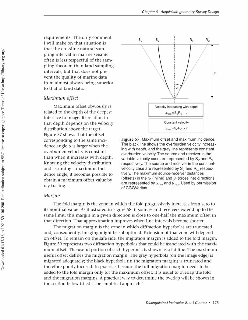
requirements. The only comment I will make on that situation is that the crossline natural sam-pling interval in marine seismic often is less respectful of the sam-pling theorem than land sampling intervals, but that does not pre-vent the quality of marine data from almost always being superior to that of land data.

Maximum offset

Maximum offset obviously is related to the depth of the deepest interface to image. Its relation to that depth depends on the velocity distribution above the target. Figure 57 shows that the offset corresponding to the same inci-dence angle α is larger when the overburden velocity is constant than when it increases with depth. Knowing the velocity distribution and assuming a maximum inci-dence angle, it becomes possible to obtain a maximum offset value by ray tracing.

Margins

The fold margin is the zone in which the fold progressively increases from zero to its nominal value. As illustrated in Figure 58, if sources and receivers extend up to the same limit, this margin in a given direction is close to one-half the maximum offset in that direction. That approximation improves when line intervals become shorter.

The migration margin is the zone in which diffraction hyperbolas are truncated and, consequently, imaging might be suboptimal. Extension of that zone will depend on offset. To remain on the safe side, the migration margin is added to the fold margin. Figure 59 represents two diffraction hyperbolas that could be associated with the maxi-mum offset. The useful portion of each hyperbola is shown as a fat line. The maximum useful offset defines the migration margin. The gray hyperbola (on the image edge) is migrated adequately; the black hyperbola (in the migration margin) is truncated and therefore poorly focused. In practice, because the full migration margin needs to be added to the fold margin only for the maximum offset, it is usual to overlap the fold and the migration margins. A practical way to determine the overlap will be shown in the section below titled “The empirical approach.”



SC SV RV

z

α

RC

Velocity increasing with depth

Constant velocity

xmax = SVRV ~ z

xmax = SCRC > z

Figure 57. Maximum offset and maximum incidence. The black line shows the overburden velocity increas-ing with depth, and the gray line represents constant overburden velocity. The source and receiver in the variable-velocity case are represented by SV and RV, respectively. The source and receiver in the constant-velocity case are represented by SC and RC, respec-tively. The maximum source-receiver distances (offsets) in the x- (inline) and y- (crossline) directions are represented by xmax and ymax. Used by permission of CGGVeritas.

Dow

nloa

ded

01/1

7/13

to 1

92.1

59.1

06.2

00. R

edis

trib

utio

n su

bjec

t to

SEG

lice

nse

or c

opyr

ight

; see

Ter

ms

of U

se a

t http

://lib

rary

.seg

.org

/

The experimental approach

The principle of an experi-mental approach is to try a set of parameters and select the param-eter set leading to the best image. In the section on noise constraints in this chapter, it was shown that the relationship between field data (elementary records) and image quality is not straightforward. Therefore, special care should be taken in the interpretation of a few elementary records before starting a high-density survey.

It does not seem reasonable to expect much from a few elemen-tary records. However, recording a few extra elementary records could be useful in confirming assump-tions in various cases. For instance, that can be done to check that the frequency spectrum at the time of the target does not fall abruptly at a frequency lower that the planned upper frequency, when the only available vintage data for the sur-vey design are band limited (vibro-seis), and improved resolution is one of the objectives of the new survey. A decision to lower the maximum sweep frequency or, most often, to keep it as intially planned then can be made.

That also can be done to compare the strength of various sources when it is necessary to mix sources in the new survey and data from only one source are available for survey design. Parameters of the other sources (charge of dyna-mite, for instance) can be adjusted.

However, selection of other parameters such as sweep length or line intervals requires more data



Migration margin

a

Imag

e ed

ge

Sur

vey

edge

Figure 59. Vertical section across the edge of a sur-vey. Angle α is the maximum angle used in migration or the maximum dip. The fat part of the diffraction hyperbolas is used to image this particular survey adequately. The gray hyperbola (on the image edge) is focused adequately. The black hyperbola (in the migra-tion margin) is truncated and poorly focused. Used by permission of CGGVeritas.

y max

ymax/2Receiver patch

Full-fold area

Single-fold area

SP

xmax

xmax/2

Figure 58. Fold margins. Top view of the edge of a survey area. If sources and receivers are both ex-tended to the edge of the survey area, the inline distance from the left or right edge to full fold is close to xmax 2 where xmax is the maximum inline offset. Sim-ilarly, the inline distance from the top or bottom edge to full fold is close to ymax 2. If line intervals are short, the fold margins are approximately half the maximum offsets in both directions. Used by permission of CGGVeritas.

Dow

nloa

ded

01/1

7/13

to 1

92.1

59.1

06.2

00. R

edis

trib

utio

n su

bjec

t to

SEG

lice

nse

or c

opyr

ight

; see

Ter

ms

of U

se a

t http

://lib

rary

.seg

.org

/

than a few records, and it takes more than a day or two to process and analyze them. In some large projects, a pilot survey can be recorded ahead of time to provide the neces-sary data (significantly more than a few records) and time (significantly more than a few days) to analyze the results adequately and use them for reasonable decisions.

In the era of 2D seismic, field tests were very popular because they could be recorded, interpreted, and processed relatively quickly. They required only a few days rather than months of data acquisition, and their cost was found to be very reasonable for the potential advantage they could bring. That time is gone.

The empirical approach

Today, seismic survey-design problems rarely are posed in areas that have not been imaged previously. Obviously, not looking at available images would be a mistake. More-over, if vintage seismic data can be accessed and manipulated, they can provide valuable assistance for the survey designer.

Illumination analysis

Conventional marine-seismic acquisition geometry is naturally anisotropic. Receivers are located in a rectangle of typical size 8 × 1 km on one side of the source. Moreover, sam-pling along the cables is different from sampling across the cables (typically 12.5 m and 50 to 100 m, respectively). Therefore, illumination will depend on the sail-line directions.

In complex cases, it could be advantageous to perform an illumination analysis. The input data needed for that analysis consist of selected horizon depths, interval velocities and, optionally, densities. They are converted into a depth model, which can be used for illumination analysis. The simplest analysis is a hit-count map (map of reflected points obtained by ray tracing). The map is limited in that it gives the same weight to rays that carry weak or strong amplitudes.

That limitation is overcome by simulated-migration-amplitude (SMA) maps, which can be computed with various degrees of sophistication. The maps can be generated for various sail-line directions and offset ranges; subsequently, they are used to select the optimal direction and maximum offset. The maps also could lead to the decision to acquire wide-azimuth data. In some cases, it becomes interesting to conduct the full modeling exercise up to migration. Figure 60 compares subbasalt images obtained from synthetic data with wide- and narrow-azimuth acquisition geometries. In this particular case, the wide-azimuth image is significantly more continuous.

Illumination analyses also can be used for land survey-design exercises. However, those analyses are more sensitive to aperture than to trace density. They do not provide much additional guidance for the choice of intervals (which are the main parameters) that are expected from land 3D designs studies. Therefore, their advantage often is not as convincing in land surveys as it is in marine, especially when the question is whether to choose narrow- or wide-acquisition geometry.

Noise conditions

A few SP displays will be useful to assess both organized and field-noise condi-tions. Recording parameters (source spectrum and field arrays in particular) must be taken into account in the assessment. Figure 61 represents three shotpoints along a



Dow

nloa

ded

01/1

7/13

to 1

92.1

59.1

06.2

00. R

edis

trib

utio

n su

bjec

t to

SEG

lice

nse

or c

opyr

ight

; see

Ter

ms

of U

se a

t http

://lib

rary

.seg

.org

/



2500

2400

2300

0SP 3550

Elevation (m)

SP 3990 SP 5060

0.5

1

1.5

2

Tim

e (s

)

2.5

3

3.5

45 km 5 km 5 km

Figure 61. Three shotpoints along a 2D line. The source consists of 5 kg of dynamite buried at 18 m. The receivers are single 3C accelerometers with a 25-m interval. Used by permission of CGGVeritas.

Figure 60. Imaging by (a) narrow-azimuth (NAZ) and (b) wide-azimuth (WAZ) data from a subba-salt model. The subbasalt image is improved significantly by WAZ geometry. Used by permission of CGGVeritas.

Dow

nloa

ded

01/1

7/13

to 1

92.1

59.1

06.2

00. R

edis

trib

utio

n su

bjec

t to

SEG

lice

nse

or c

opyr

ight

; see

Ter

ms

of U

se a

t http

://lib

rary

.seg

.org

/

line in a mountainous area. The source is a single charge of 5 kg of explosives buried at a depth of 18 m. The receivers are single 3C sensors. The group interval is 25 m. The processing applied is a multiplication by t2.5 to compensate approximately for spherical divergence and absorption losses and application of static corrections. Reflections can be seen down to 2.5 s, except below the highest elevations in the center of the line. Ground roll does not appear as a major problem. Ambient noise is relatively high.

Frequency content

Narrow bandpass filters applied to the above shotpoints will help to refine the analysis (ground-roll velocity and bandwidth and field-noise bandwidth). Figure 62 represents such an analysis applied to SP 5060 of Figure 61. Below 7 Hz, reflections are hidden by ground roll and ambient noise, and 80 Hz can be seen in the first second of data.



5 Hz0

1

2

Tim

e (s

)

3

Offset (km) Offset (km) Offset (km) Offset (km) Offset (km)2 4 6 2 4 6 2 4 6 2 4 6 2 4 6

7 Hz 10 Hz 14 Hz 20 Hz

28 Hz

Tim

e (s

)

Offset (km) Offset (km) Offset (km) Offset (km) Offset (km)2 4 6 2 4 6 2 4 6 2 4 6 2 4 6

40 Hz 56 Hz 80 Hz 112 Hz

Figure 62. Frequency analysis of field data. Ten narrow-bandpass filters are applied to SP 5060 of Figure 61. The panels are labeled with the center frequency of the filter. They are gained as fol-lows: 5 Hz (9 dB), 7 Hz (6 dB), 10 Hz (3 dB), 14 Hz (0 dB), 20 Hz (0 dB), 28 Hz (0 dB), 40 Hz (3 dB), 56 Hz (6 dB), 80 Hz (9 dB), 112 Hz (12 dB). Used by permission of CGGVeritas.

Dow

nloa

ded

01/1

7/13

to 1

92.1

59.1

06.2

00. R

edis

trib

utio

n su

bjec

t to

SEG

lice

nse

or c

opyr

ight

; see

Ter

ms

of U

se a

t http

://lib

rary

.seg

.org

/

The same exercise can be applied to a stack section. A wavelet extracted in the zone of interest might bring additional information. Figure 63 shows a way to extract the wavelet. An event is picked on a selected data set. Figure 63a shows the brute stack. The selected event is the reflection at 1.85 s. It is time-aligned and normalized (Figure 63b). The wavelet shown in Figure 63c is the average of data in Figure 63b after time alignment, windowed around the zone of interest. Figure 63d represents the amplitude spectrum of the wavelet. No frequency above 50 Hz can be seen at this depth. The limitation of this frequency content can have several causes, and it is the task of the designer to sort them out:

high noise contamination (Figure 62)• inadequate sweep parameters (if the spectrum of the wavelet looks truncated at the • sweep-limit frequencies) insufficient source strength. Increasing source strength at a given frequency will • increase the S/N at that frequency if noise is not source-generated. A way to assess whether the noise is generated by source (scattering) is to look at constant-gain data (no spherical-divergence compensation).absorption. Looking at how the amplitude decreases with frequency can provide • information on absorption.processing problem. A poor static solution or incorrect velocities could be mistaken • as high absorption. If there is a good reason to believe that processing can be improved, it could be a mistake not to reprocess some data.

Maximum offset

Looking at a CMP gather or a supergather can help to define the maximum usable offset. Figure 64 represents a supergather obtained by selecting 50 CMPs in an area of relatively flat reflectors, applying NMO corrections, and averaging traces with



c) d) 30

20

10

0

–10

–20

–300 20 40 60

Frequency (Hz)

Am

plitu

de (

dB)

80 100 120

1.2

a) b)

1.4

1.6

Tim

e (s

)

1.8

2.0

625 m 625 m

Figure 63. Frequency-content evaluation by wavelet analysis. (a) Brute stack. Selection of a reflec-tor at 1.85 s. (b) Reflector flattening and normalization. (c) Wavelet = average of flattened reflector and windowing. (d) Amplitude spectrum of wavelet. Used by permission of CGGVeritas.

Dow

nloa

ded

01/1

7/13

to 1

92.1

59.1

06.2

00. R

edis

trib

utio

n su

bjec

t to

SEG

lice

nse

or c

opyr

ight

; see

Ter

ms

of U

se a

t http

://lib

rary

.seg

.org

/

similar offsets. This large averaging is necessary because of poor data quality. In general, fewer CMPs need to be averaged. Offsets as great as 6 km are useful in imaging the reflection at 2.4 s.

Survey margins

Information on margins is one important thing survey designers can obtain from vintage data. A simple evaluation can be made if prestack data are available. The desired image limit (if vintage data cover it) or fictive image limit is defined on a migrated section. The limit must be far enough from the vintage section edge to ensure that optimum imaging is obtained. A few prestack survey limits can be simulated by selecting the appropriate sources and receivers in the vintage data and then forming the corresponding stack sections and migrating them (Figure 65). The full



0

0.5

1

1.5

Tim

e (s

)

2

2.5

3–6000 –4000 –2000 0

Offset (m)2000 4000 6000

Figure 64. Supergather formed by averaging 50 consecutive CMPs along a 2D line in an area that has nearly horizontal reflectors. This large averaging is necessary to observe the reflector at 2.4 s. Used by permission of CGGVeritas.

0

1

Tim

e (s

)

2

30 1250

1500 ma) b) c) d)1250 mMigration margin

1000 m 750 m

x (m)2500 0 1250

x (m)2500 0 1250

x (m)2500 0 1250

x (m)2500

Figure 65. Migration-margin evaluation. (a) Full-line migration is compared with the migrations obtained from (b through d) three simulations of line end. The simulations extend (b) 1250 m, (c) 1000 m, and (d) 750 m past the fault interpreted in black. Used by permission of CGGVeritas.

Dow

nloa

ded

01/1

7/13

to 1

92.1

59.1

06.2

00. R

edis

trib

utio

n su

bjec

t to

SEG

lice

nse

or c

opyr

ight

; see

Ter

ms

of U

se a

t http

://lib

rary

.seg

.org

/

line migration is shown in Figure 65a. The fault interpreted in white must be imaged properly. Three simulations of line truncation have been constructed in Figure 65b through 65d. They extend 1250, 1000, and 750 m, respectively, past the fault. The shorter margins do not allow adequate imaging of the fault.

In all cases, it must be remembered that vintage data were acquired with methods and equipment different than what will be used for the new survey. The most frequent difference (and probably the most difficult to account for fully) occurs when vintage data are in two dimensions and new data will be in three dimensions. For that reason, it is always necessary to weight the results obtained from this analysis with theoretical results. Finding the right weight is the key, and it is essentially a matter of experience.

Conclusion

Survey design makes a necessary compromise between economic constraints and the main causes of imperfection of the seismic image — noise contamination, inad-equate sampling and limited size of the measurement surface, and measurement and processing errors.

It is remarkable that the effect of the first two causes can be mitigated by the same remedy — interval reduction. The interval between sensors or source elements must be less than about 80% of the shortest noise wavelength. The interval between source and receiver stations must be less than half the minimum apparent velocity divided by the maximum desired frequency. The interval between source lines and receiver lines must be short enough so that it does not jeopardize prestack migration. That interval also must be as short as possible when noise cannot be attenuated satisfactorily by noise-reduction techniques other than stack and migration.



Dow

nloa

ded

01/1

7/13

to 1

92.1

59.1

06.2

00. R

edis

trib

utio

n su

bjec

t to

SEG

lice

nse

or c

opyr

ight

; see

Ter

ms

of U

se a

t http

://lib

rary

.seg

.org

/

6. Chapter 6 Acquisition-geometry Survey Design

Documents

surveydesign problem

d surveydesign workshop

original sin of survey

adequate image

short wavelengths

seismic data

noise wavelengths

common acquisition geometries