5D-BESS2

Five dimensional formulation of the Degenerate BESS model

Francesco Coradeschi, Stefania De Curtis and Daniele Dominici

Department of Physics, University of Florence,

and INFN, Via Sansone 1, 50019 Sesto F., (FI), Italy

(Dated: January 14, 2010)

We consider the continuum limit of a moose model corresponding to a generalization

to N sites of the Degenerate BESS model. The five dimensional formulation emerging

in this limit is a realization of a RS1 type model with SU(2)L⊗SU(2)R in the bulk,

broken by boundary conditions and a vacuum expectation value on the infrared

brane. A low energy effective Lagrangian is derived by means of the holographic

technique and corresponding bounds on the model parameters are obtained.

I. INTRODUCTION

The exact nature of the mechanism that leads to the breakdown of the electroweak (EW)

symmetry is one of the relevant open questions in particle physics. While waiting for the first

experimental data from the Large Hadron Collider, it is worthwhile to explore the potential

electroweak breaking scenarios from a theoretical point of view.

In the Standard Model (SM), the mechanism of the EW symmetry breaking implies the

presence a fundamental scalar particle, the Higgs boson, with a light mass as suggested by

EW fits. However, this mechanism is affected by a serious fine-tuning problem, the hierarchy

problem, because the mass of the Higgs boson is not protected against radiative corrections

and would naturally be expected to be as large as the physical UV cut-off of the SM, which

could be as high as MP ' 1019 GeV.

Possible solutions to the hierarchy problem are the technicolor (TC) theories [1–3]

(that postulate the presence of new strong interactions around the TeV scale) and extra-

dimensional theories [4–6]. These seemingly unrelated classes of theories have in fact a

profound connection through the AdS/CFT correspondence [7]. According to this conjec-

ture, five dimensional (5D) models on AdS space are “holographic duals” to 4D theories with

spontaneously broken conformal invariance. The duality means that when the 5D theory is

in a perturbative regime the holographic dual is strongly interacting and vice versa. This

2

fact provides an unique tool to make quantitative calculations in 4D strongly interacting

theories, and creates a very interesting connection between extra-dimensional and TC-like

theories.

Working in the framework suggested by the AdS/CFT correspondence, one considers

for the fifth dimension a segment ending with two branes (one ultraviolet, UV, and the

other one infrared, IR). Several choices of gauge groups in the bulk have been proposed:

there are models, with or without the Higgs, which assume a SU(2)L × SU(2)R × U(1)B−L

gauge group, [8–17], or SU(2) × U(1) [18–21] or a simpler SU(2) in the 5D bulk. [22, 23].

Compactification from five to four dimensions is often performed by the standard Kaluza

Klein mode expansion, however alternative methods have been suggested. Effective low

energy chiral Lagrangians in four dimensions, can be obtained by holographic versions of

5D theories in warped background [24–26] or via the deconstruction technique [27–35]. The

deconstruction mechanism provides a correspondence at low energies between theories with

replicated 4D gauge symmetries G and theories with a 5D gauge symmetry G on a lattice.

We will refer to the deconstructed models also as moose models. Several examples mainly

based on the gauge group SU(2) have recently received attention [36–44]. It is interesting to

note that even few sites of the moose give a good approximation of the 5D theory [45]. The

BESS model [46, 47], based on the symmetry SU(2)3, is a prototype of models of this kind:

with a particular choice of its parameters it can generate the recently investigated three site

model [48–52].

Generic TC models usually have difficulties in satisfying the constraints coming from EW

precision measurements on S, T, U observables [53, 54]. In this paper, we have reconsidered

the Degenerate BESS (D-BESS) model [55, 56], a low-energy effective theory which possesses

a (SU(2)⊗ SU(2))2 custodial symmetry that leads to a suppressed contribution from the

new physics to the EW precision observables, making possible to have new vector bosons

at a relatively low energy scale (around a TeV). This new vector states are interpreted as

composites of a strongly interacting sector. Starting from the generalization to N sites of

the D-BESS model (GD-BESS) [38, 57], based on the deconstruction or “moose” technique

[27], we consider the continuum limit to a 5D theory.

The D-BESS model and its generalization suffer the drawback of the unitarity constraint,

which is as low as that of the Higgsless SM [58, 59], that is around 1.7 TeV. However,

(at least for a particular choice of the extra-dimensional background) in the 5D model it

3

is meaningful to reintroduce an Higgs field, delaying unitarity violation to a scale & 10

TeV. In the “holographic” interpretation of AdS5 models [60, 61], inspired by the AdS/CFT

correspondence, this Higgs can be thought as a composite state and thus does not suffer from

the hierarchy problem. The 5-dimensional D-BESS (5D-DBESS) on AdS5 then provides a

coherent description of the low energy phenomenology of a new strongly interacting sector

up to energies significantly beyond the ∼ 2 TeV limit of the Higgsless SM, still showing

a good compatibility with EW precision observables. While studying this 5D extension,

furthermore, we have clarified a not-so-obvious fact: there is at least a particular limit,

where the 5D-DBESS can be related to a realization of the RS1 model [5], specifically the

one proposed in ref. [20].

In Section II we review the generalization of D-BESS to N sites. In Section III we

extend the model to five dimensions clarifying how the boundary conditions at the ends

of the 5D segment emerge from the deconstructed version of the model. The 5D model is

described by a SU(2)L×SU(2)R bulk Lagrangian with boundary kinetic terms, broken both

spontaneously and by boundary conditions. In Section IV we develop the expansion in mass

eigenstates consisting in two charged gauge sectors, left (including W ) and right, and one

neutral (including the photon and the Z). We also get obtain the expanded Lagrangian for

the modes. In Section V we derive the low energy Lagrangian by means of the holographic

technique and the EW precision parameters ε1,2,3. In Section VI we show the spectrum

of KK excitations and derive the bounds from EW precision measurements on the model

parameters for two choices of the 5D metric, the flat case and the RS one. Conclusions are

given in Section VII. In Appendix A, by following [62, 63], we develop the technique for

Kaluza-Klein expansion.

II. REVIEW OF THE GD-BESS MODEL

The GD-BESS model is a moose model with a [SU(2)]2N ⊗ SU(2)L ⊗ U(1)Y gauge sym-

metry, described by the Lagrangian [57]:

L =2N+1∑

i=1,i 6=N+1

f 2i Tr[DµΣ†

iDµΣi] + f 2

0 Tr[DµU†DµU ]

− 1

2g2Tr[(FW

µν)2]− 1

2g′2Tr[(FB

µν)2]− 1

2g2i

2N∑i=1

Tr[(Fiµν)

2],

(1)

4

Σ1

SU(2)L

Σ2 Σ2N Σ2N+1

U(1)Y

G1 GN GN+1 G2N

U

FIG. 1: Graphic representation of the moose model described by the Lagrangian given in Eq. (1).

The dashed lines represent the identification of the corresponding moose sites.

where

Fiµν = ∂µA

iν − ∂νA

iµ + i[Aµ,Aν ], i = 0, . . . 2N + 1 (2)

with Ai ≡ Aa i τa

2, i = 1, . . . 2N are the [SU(2)]2N gauge fields, A0 ≡ W ≡ W a τa

2and

A2N+1 ≡ B ≡ B τ3

2are the SU(2)L⊗U(1)Y gauge fields, and the chiral fields Σi and U have

covariant derivatives defined by

DµΣi = ∂µΣi + iAi−1µ Σi − iΣiAi

µ, i = 1, . . . 2N + 1, i 6= N + 1 (3)

DµU = ∂µU + iWµ U − iU Bµ (4)

The model has two sets of parameters, the gauge coupling constants g, g′, gi, i = 1, . . . 2N ,

and the “link coupling constants” fi, i = 1, . . . 2N + 1, i 6= N + 1. For simplicity, we will

impose a reflection invariance with respect to the ends of the moose, getting the following

relations among the model parameters

fi = f2N+2−i, gi = g2N+1−i. (5)

The model content in terms of fields and symmetries can be summarized by the moose in

Fig. 1.

The most peculiar feature is the absence in the Lagrangian given in Eq. (1) of any field

connecting the N th and the N + 1th sites of the moose. This situation was referred to in ref.

[38] as “cutting a link”. As it was shown there, this choice guarantees the vanishing of the

leading order corrections from new physics to the EW precision parameters; for instance,

in ref. [57], the contributions to the ε parameters [64–66] as well as the “universal” form

5

factors [26] were calculated, showing that all these contributions are of order m2Z/M2, where

M is the mass scale of the lightest new resonance in the theory.

III. GENERALIZATION TO 5 DIMENSIONS

We now want to describe the continuum limit N →∞ of the Lagrangian given in Eq. (1).

As it is well known, a [SU(2)]K linear moose model can be interpreted as the discretized

version of a SU(2) 5D gauge theory. The GD-BESS model, however, has a number of

new features with respect to a basic linear moose. In particular, we have the “cut link”

and the presence of an apparently nonlocal field U which connects the gauge fields of the

SU(2)L ⊗ U(1)Y local symmetry.

To be able to properly describe the 5D generalization, we need a representation for the

5D metric. Since the deconstructed model possesses ordinary 4D Lorentz invariance, the

extra-dimensional metric must be compatible with this symmetry. Such a metric can in

general be written in the form:

ds2 = b(y)ηµν dxµdxν + dy2, (6)

where η is the standard Lorentz metric with the (−, +, +, +) signature choice, y the variable

corresponding to the extra dimension and b(y) is a generic positive definite function, usually

known as the “warp factor”. We normalize b(y) by requiring that b(0) = 1. For definiteness,

we will consider a finite extra dimension, with y ∈ (0, πR). With this choice, it is possible

to write down an identification between the GD-BESS and the continuum limit parameters:

g2i

N→ g2

5

πR, f 2

i → b(y)N

πRg25

, (7)

where g5 is a 5D gauge coupling, with mass dimension −1/2. As can be seen, a general choice

for the gi implies that g5 is “running” , with an explicit dependence on the extra variable.

In the following, we will not consider this possibility, but rather restrict for simplicity to a

constant coupling (as it is standard in the literature), so, from the 4D side, we will have

gi ≡ gc.

The trickiest part of the generalization, however, is to interpret the cutting of the link.

To understand this properly, we can start by noticing that the cut link prevents any direct

contact between the two sides of the moose; the fields on the left only couple to those on the

6

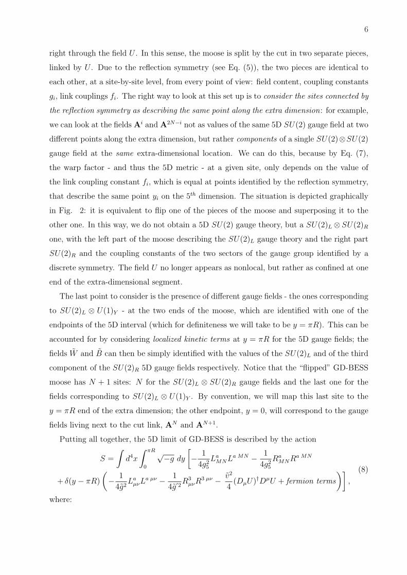
right through the field U . In this sense, the moose is split by the cut in two separate pieces,

linked by U . Due to the reflection symmetry (see Eq. (5)), the two pieces are identical to

each other, at a site-by-site level, from every point of view: field content, coupling constants

gi, link couplings fi. The right way to look at this set up is to consider the sites connected by

the reflection symmetry as describing the same point along the extra dimension: for example,

we can look at the fields Ai and A2N−i not as values of the same 5D SU(2) gauge field at two

different points along the extra dimension, but rather components of a single SU(2)⊗SU(2)

gauge field at the same extra-dimensional location. We can do this, because by Eq. (7),

the warp factor - and thus the 5D metric - at a given site, only depends on the value of

the link coupling constant fi, which is equal at points identified by the reflection symmetry,

that describe the same point yi on the 5th dimension. The situation is depicted graphically

in Fig. 2: it is equivalent to flip one of the pieces of the moose and superposing it to the

other one. In this way, we do not obtain a 5D SU(2) gauge theory, but a SU(2)L⊗ SU(2)R

one, with the left part of the moose describing the SU(2)L gauge theory and the right part

SU(2)R and the coupling constants of the two sectors of the gauge group identified by a

discrete symmetry. The field U no longer appears as nonlocal, but rather as confined at one

end of the extra-dimensional segment.

The last point to consider is the presence of different gauge fields - the ones corresponding

to SU(2)L ⊗ U(1)Y - at the two ends of the moose, which are identified with one of the

endpoints of the 5D interval (which for definiteness we will take to be y = πR). This can be

accounted for by considering localized kinetic terms at y = πR for the 5D gauge fields; the

fields W and B can then be simply identified with the values of the SU(2)L and of the third

component of the SU(2)R 5D gauge fields respectively. Notice that the “flipped” GD-BESS

moose has N + 1 sites: N for the SU(2)L ⊗ SU(2)R gauge fields and the last one for the

fields corresponding to SU(2)L ⊗ U(1)Y . By convention, we will map this last site to the

y = πR end of the extra dimension; the other endpoint, y = 0, will correspond to the gauge

fields living next to the cut link, AN and AN+1.

Putting all together, the 5D limit of GD-BESS is described by the action

S =

∫d4x

∫ πR

0

√−g dy

[− 1

4g25

LaMNLa MN − 1

4g25

RaMNRa MN

+ δ(y − πR)

(− 1

4g2La

µνLa µν − 1

4g′2R3

µνR3 µν − v2

4(DµU)†DµU + fermion terms

)],

(8)

where:

7

Σ1

SU(2)L

Σ2 Σ2N Σ2N+1

U(1)Y

G1 GN GN+1 G2N

U

⇓ΣN+2

y = 0

Σ2N−2 Σ2N−1 Σ2N Σ2N+1

U y = πR

ΣN Σ4 Σ3 Σ2 Σ1

GN+1 G2N−2 G2N−1 G2N

U(1)Y

GN G3 G2 G1

SU(2)L

FIG. 2: Interpretation of the cut link in the continuum limit of the GD-BESS model. The first

half of the moose is “flipped” and superimposed to the second half. In this way, the N th and the

N + 1th sites are identified with the y = 0 brane, while the 1st and the 2N + 1th with the y = πR

one.

• with the usual convention, the greek indices run from 0 to 3, while capital latin ones

take the values (0, 1, 2, 3, 5), with “5” labelling the extra direction

• g is the determinant of the metric tensor gMN , defined by

ds2 = gMNdxMdxN ≡ b(y) ηµνdxµdxν + dy2, (9)

• LaMN and Ra

MN are the SU(2)L ⊗ SU(2)R gauge field strengths:

L(R)aMN = ∂MW a

L(R) N − ∂NW aL(R) M + iεabcW b

L(R) MW cL(R) N ; (10)

the fields W aL(R) represent the continuum limit of the Aa i

• g, g′, g5 are three, in general different, gauge couplings. g and g′ are the direct

analogous of their deconstructed counterparts. g5 is the bulk coupling, it has mass

dimension −12, and it is the 5D limit of the gi, as can be seen by Eq. (7)

8

• the brane scalar U is a SU(2)-valued field, with its covariant derivative defined by:

DµU = ∂µU + iW aL µ

τa

2U − iW 3

R µUτ 3

2, (11)

in exact analogy with Eq. (4). Note that the field U is analogous to the one that

describes the standard Higgs sector in the limit of an infinite Higgs mass [58]. It can

be conveniently parametrized in terms of three real pseudo-scalar fields πa,

U = exp(iπaτa

2v); (12)

• the fermionic terms, which we take to be confined on the brane for simplicity, have

the usual SM form.

It is important to notice that the action (8) does not define the physics of the model

uniquely: we still have the freedom of choosing boundary conditions (BCs) for the fields.

This BC ambiguity is absent in deconstructed models: the BCs get implicitly specified by

the way in which the discretization of the 5th dimension is realized. This means that the

GD-BESS model described by Eq. (1) already has a specific set of “built-in” BCs. These

can be understood by looking at the residual gauge symmetry at the ends of the moose. It

is apparent that, after the “flipping” depicted in Fig. 2, at the N th and (N + 1)th sites,

corresponding to y = 0 in the continuum limit, we have the full SU(2)L ⊗ SU(2)R gauge

invariance. By contrast, at the 0th and (2N +1)th sites, corresponding to y = πR, the gauge

symmetry is broken down to SU(2)L⊗U(1)Y . To do this, we have to impose Dirichlet BCs

on two of the SU(2)R gauge fields at y = πR, while all the other fields, and all the fields at

y = 0 are unconstrained. The complete gauge symmetry breaking pattern is thus as follows:

we have a SU(2)L⊗SU(2)R gauge invariance in the bulk, unbroken on the y = 0 brane and

broken by a combination of Dirichlet BCs and scalar VEV (of the U field) to U(1)e.m. on

the y = πR brane.

In the following of this work, we will study the model defined by the action (8). First

of all, we will perform a general analysis of the full 5D theory by the standard technique

of the Kaluza-Klein (KK) expansion. Then we will look at the low-energy limit and derive

expression for the ε parameters; the results will confirm that this is indeed the 5D limit

of GD-BESS. Finally, we will make some remarks on the phenomenology of the model in

correspondence with two interesting choices for the geometry of the 5th dimension, that of

a flat dimension (b(y) ≡ 1) and that of a slice of AdS5 (b(y) = e−2ky).

9

IV. EXPANSION IN MASS EIGENSTATES

Since we wish to keep the metric generic for the moment, a convenient strategy is to

expand the gauge fields W aL(R) M (and the goldstones πa) directly in terms of mass eigenstates

[62, 63]. So we define:

W aL µ(x, y) =

∞∑j=0

faL j(y) V (j)

µ (x), W aL 5(x, y) =

∞∑j=0

gaL j(y) G(j)(x),

W aR µ(x, y) =

∞∑j=0

faR j(y) V (j)

µ (x), W aR 5(x, y) =

∞∑j=0

gaR j(y) G(j)(x),

πa(x) =∞∑

j=0

caj G(j)(x).

(13)

The expansion (13) is written in full generality. A priori, this means that fields with

different SU(2) index could be mixed. The index “(j)” labels all the mass eigenstates. This

procedure is in fact more general than it is needed; we will see that, with our choice of

BCs for the model, we will get three decoupled towers of eigenstates, so that many of the

above wave-functions (or constant coefficients in the case of the brane pseudo-scalars) are

vanishing. We will require that the wave-functions in eq.(13) form complete sets, and that

after substituting the expansion and performing the integration over the extra-dimensional

variable y, a diagonal bilinear Lagrangian result, i.e. the fields defined in eq. (13) are the

mass eigenstates. These requests lead to an equation of motion plus a set of BCs that the

profiles must satisfy. Details on the derivation are given in Appendix A; here we only report

the results.

Since the proof of the diagonalization is somewhat technical, we will proceed in reverse

order, first defining the three sectors of the model, together with the conditions that the

corresponding wave-functions have to satisfy, then show how the three sectors are derived

by the request of diagonalizing the KK expanded Lagrangian. The three sectors are:

• A left charged sector coming from the expansion of the (W 1, 2L )M fields and the brane

10

pseudo-scalars π1,2. The explicit form of the expansion is

W 1,2L µ(x, y) =

∞∑n=0

f 1,2L n(y) W

1,2 (n)L µ (x),

W 1,2L 5(x, y) =

∞∑n=0

g1,2L n(y) G

1,2 (n)L (x),

π1,2(x) =∞∑

n=0

c1,2n G(n)(x).

(14)

The wave-functions of the vector fields satisfy the equation of motion:

Df 1,2L n = −m2

L nf 1,2L n, (15)

where we defined the differential operator:

D ≡ ∂y(b(y)∂y(·)), (16)

and the set of BCs:

∂yf1,2L n = 0 at y = 0, (17)

(g2

g25∂y − b(πR) m2

L n + g2v2

4

)f 1, 2

L n = 0 at y = πR. (18)

The pseudo-scalar profiles are fixed by the conditions:

g1,2L n =

1

mL n

∂yf1,2L n, c1, 2

n =v

2mL n

f 1, 2L n

∣∣πR

. (19)

Note that in this sector no massless solution is allowed; in fact, eq. (15) together with

the Neumann BC at y = 0 (17) imply that a massless mode must have a constant

profile, and a constant, massless solution cannot satisfy the BC at y = πR (18). Also

note that eq. (15) and the BCs (17) and (18) are diagonal in the isospin index, so we

have f 1L n = f 2

L n.

Some caution must be used in writing down the completeness and orthogonality re-

lations for the f 1,2L n mode functions. The differential operator D (16) is in fact not

hermitian with respect to the ordinary scalar product when evaluated on functions

obeying BCs of the kind (18), due to the presence of terms explicitly containing the

eigenvalues mL n which are induced by πR-localized terms in the action. To obtain the

11

correct completeness and orthogonality properties of this function set, a generalized

scalar product must be used which takes into account such terms. This is given by

(f 1, 2

L n , f 1, 2L m

)g

= L2mδmn, (f, h)g =

1

g25

∫ πR

0

dy fh +1

g2fh|πR , (20)

where Lm sets the normalization. Since the scalar product (·, ·)g is dimensionless, we

will set: Lm ≡ 1. This will ensure that the kinetic terms of the bosons of this sector

are canonically normalized. From this definition we deduce the completeness relation:

1

g25

∑

k

f 1, 2L k (y)f 1, 2

L k (z) +1

g2δ(z − πR)

∑

k

f 1, 2L k (y)f 1, 2

L k (πR) = δ(y − z); (21)

• A right charged sector coming from the expansion of (W 1, 2R )M . The explicit form of

the expansion for this sector is

W 1,2R µ(x, y) =

∞∑n=0

f 1,2R n(y) W

1,2 (n)R µ (x),

W 1,2R 5(x, y) =

∞∑n=0

g1,2R n(y) G

1,2 (n)R (x).

(22)

The wave-functions of the vector fields satisfy a similar equation of motion:

Df 1,2R n = −m2

R nf1,2R n, (23)

and the set of BCs:

∂yf1,2R n = 0 at y = 0, (24)

f 1,2R n = 0 at y = πR. (25)

The scalar profiles are given by:

g1,2R n =

1

mR n

∂yf1,2R n. (26)

Again, in this sector there is no massless solution, for the constant profile of a massless

mode is incompatible with the BC (25). Also, the equation of motion and the BCs

are again diagonal in the isospin index, so f 1R n = f 2

R n. The right charged sector obeys

the usual L2 orthogonality property:

(f 1, 2

R n , f 1, 2R m

) ≡ 1

g25

∫ πR

0

dy f 1, 2R nf 1, 2

R m = R2mδmn, (27)

where the factor 1/g25 has been inserted to compensate for the mass dimension of the

integral, so that we can normalize: Rm ≡ 1, again ensuring that the kinetic terms will

have the canonical normalization.

12

• Finally, a neutral sector coming from the expansion of (W 3L)M , (W 3

R)M and π3. The

expansion has the form

W 3L µ(x, y) =

∞∑n=0

f 3L n(y) N (n)

µ (x), W 3L 5(x, y) =

∞∑n=0

g3L n(y) G

(n)N (x),

W 3R µ(x, y) =

∞∑n=0

f 3R n(y) N (n)

µ (x), W 3R 5(x, y) =

∞∑n=0

g3R n(y) G

(n)N (x),

π3(x) =∞∑

j=0

c3j G(j)(x);

(28)

the equation of motion and the BCs for the vector profiles are given by:

Df 3L,R n = −m2

N nf3L,R n, (29)

∂yf3L,R n = 0 at y = 0, (30)

(g2

g25∂y − b(πR) m2

N n + g2v2

4

)f 3

L n − g2v2

4f 3

R n = 0(

g′2

g25∂y − b(πR) m2

N n + g′2v2

4

)f 3

R n − g′2v2

4f 3

L n = 0at y = πR, (31)

and the pseudo-scalar profiles satisfy

g3L,R n =

1

mN n

f 3L,R n, if mN n 6= 0

g3L,R n = 0 if mN n = 0 (32)

c3n =

v

2mn

(f 3

L n − f 3R n

)∣∣πR

.

In contrast with the charged ones, the neutral sector admits a single massless solution;

we have mN 0 = 0. Eqs. (29) and (30) imply for a massless mode that both f 3L n and

f 3R n must be constant; then, using also eq. (31) we get:

f 3L 0 = f 3

R 0 ≡ f0, (33)

where f0 is a constant. The massless mode has to be identified with the photon

⇒ N(0)µ ≡ Aµ; since it is the only massless mode in the spectrum we have that the

symmetry of the vacuum is, correctly, just U(1)e.m.. The “charged” and “neutral”

labels we have given to the three sectors refer to their transformation properties with

respect to this unbroken symmetry.

As in the case of the left charged sector, the BCs at y = πR in this case explicitly

contain the mass of the nth mode, so that again the basis wave-functions f 3L n and f 3

R n

13

have nonstandard orthogonality properties. The correct relations are:

(f 3

L n, f3L m

)g

= (NLm)2δmn,

(f 3

R n, f3R m

)g′ = (NR

m)2δmn, (34)

where (·, ·)g′ is defined in a way analogous to (·, ·)g (eq. (20)). Completeness relations

similar to that in eq. (21) also hold. Note that it is not possible to set both NLn and

NRn to 1. In fact, since they obey the same differential equation (29) and the same BC

at y = 0 (30), f 3L n and f 3

R n are proportional to each other:

f 3L n = Knf 3

R n, (35)

and the constants Kn are fixed by the BCs at y = πR (31). To get, also in this case,

canonically normalized kinetic terms we have to set:

(NLn )2 + (NR

m)2 = 1; (36)

the ratio (NLn )/(NR

n ) will be fixed by the value of Kn and by eq. (34). In particular,

for the massless mode it is easy to get

1

f 20

=2πR

g25

+1

g2+

1

g′2. (37)

A. The expanded Lagrangian

After the expansion in mass eigenstates, the gauge Lagrangian, taking into account con-

tributions from both brane and bulk terms, is reduced to the form:

Lgauge =− 1

2W

+(n)L µν W

− (n) µνL − 1

2W

+(n)R µν W

− (n) µνR − 1

4N (n)

µν N (n) µν

−∣∣∣∂µG

+(n)L −mL nW

+(n)L µ

∣∣∣2

−∣∣∣∂µG

+(n)R −mR nW

+(n)L µ

∣∣∣2

− 1

2

(∂µG

(n)N −mN nN

(n)µ

)2

+

{i gL

klm

[N (m)

µν W+(k) µL W

− (l) νL + N (m)

µ (W− (l) µνL )W

+(k)L ν − h.c.)

]

+ g2 LLklmn

[W

+(k) µL W

− (l) νL W

+ (m) ρL W

− (n) σL (ηµρηνσ − ηµνηρσ)

]

+ g2 LNklmn

[W

+(k) µL W

− (l) νL N (m) ρN (n) σ(ηµρηνσ − ηµνηρσ)

]+ (L ↔ R)

}.

(38)

14

The bilinear part of the Lagrangian is, as announced, diagonal. The trilinear and quadrilin-

ear coupling constants gLklm, g2 LL

klmn, g2 LNklmn are defined in terms of the gauge profiles:

gLklm =

1

g25

∫ πR

0

dyf 1L kf

1L lf

3L m +

1

g2f 1

L kf1L lf

3L m|πR, (39)

g2 LLklmn =

1

g25

∫ πR

0

dyf 1L kf

1L lf

1L mf 1

L n +1

g2f 1

L kf1L lf

1L mf 1

L n|πR, (40)

g2 LNklmn =

1

g25

∫ πR

0

dyf 1L kf

1L lf

3L mf 3

L n +1

g2f 1

L kf1L lf

3L mf 3

L n|πR (41)

(remember that f 1L(R) n ≡ f 2

L(R) n); similar definitions hold for the coupling constants

gRklm, g2 RR

klmn , g2 RNklmn of the right sector, but without any contribution from boundary terms

due to eq. (25).

An important observation concerns the couplings gL(R)kl0 . These give the coupling of N (0) ,

which we identified with the photon, with the charged fields; as a consequence, they should

all be equal to the electric charge, for any value of k, l. By the definition (39) and eq. (33),

we immediately get:

gLkl0 = gR

kl0 ≡ f0δkl, (42)

thanks to the fact that the wave-functions f 1L k and f 1

R k form an orthonormal basis. Then

we conclude that

f0 = e. (43)

Then, from Eq. (37), we derive an expression for the electric charge as a function of the

model parameters:1

e2=

2πR

g25

+1

g2+

1

g′2. (44)

The actual profiles and masses can of course only be obtained by specifying the warp

factor b(y). However, it is possible to write, in general, the equations from (14) to (32)) in

a more compact form. In fact, equations of motion (15), (23) and (29) all have the same

form, Df = −m2f . This is a second order ODE, so it admits two independent solutions.

Following ref. [63], we can introduce two convenient linear combinations C(y, mn) and

S(y,mn) (“warped sine and cosine”) such that

C(0,m) = 1, ∂yC(0,m) = 0; S(0,m) = 0, ∂yS(0,m) = m (45)

with m 6= 0 (we have already seen that there is a single massless mode and that its profile

is constant). In the limit of a flat extra dimension, these functions reduce to the ordinary

sine and cosine.

15

Thanks to the Neumann BCs on the y = 0 brane (17), (24), (30), the vector profiles

faL,R n are all proportional to C(y, mn). The eigenvalues, that is the physical masses of the

vector fields mL n, mR n and mN n, are then fixed by the BCs on the IR brane (18), (25) and

(31). For the three sectors we can easily derive three eigenvalue equations:

Left charged:

g2

g25C ′(πR, mL n)− (b(πR) m2

L n − g2v2

4) C(πR, mL n) = 0 (46)

Right charged:

C(πR, mR n) = 0 (47)

Neutral:

(g2

g25C ′(πR,mN n)− (b(πR) m2

N n − g2v2

4) C(πR, mN n)

)·

(g′2

g25C ′(πR, mN n)− (b(πR) m2

N n − g′2v2

4) C(πR, mN n)

)

= g2g′2v4

16C(πR,mN n)2

(48)

In section VI we will make extensive use of these equations for specific choices of the warp

factor and of the parameters of the models to obtain explicit examples of the KK spectrum.

V. LOW ENERGY LIMIT AND EW PRECISION OBSERVABLES

We can obtain a convenient low-energy approximation of the theory by using the so-

called holographic approach [25, 60, 61, 67–70], which consists in integrating out the bulk

degrees of freedom in the functional integral. For the purposes of the present calculation it

is sufficient to take into account just the tree-level effects of the heavy resonances, so the

integration can be done by simply eliminating the bulk fields from the Lagrangian via their

classical equations of motion; moreover, bulk gauge self-interactions can be neglected.

The equations to be solved are:

D W aL(R) µ(p, y) = (p2δµν − pµpν)W

a νL(R)(p, y) (49)

with D defined in eq. (16)) and we have Fourier transformed with respect to the first four

coordinates. As previously discussed, on the y = 0 brane, we do not want to make any

16

assumptions on the value of the fields; so we leave their variations arbitrary, and since there

are no localized terms on the brane, this leads to Neumann boundary conditions for all of

the fields:

∂yWaL µ = 0

∂yWaR µ = 0

y = 0. (50)

At the other end of the AdS segment, we account for the presence of localized terms by

imposing four fields to be equal to generic source fields, while the other two (those corre-

sponding to the right charged sector) are vanishing:

W aL µ = W a

µ

W 3R µ = Bµ

W 1,2R µ = 0

y = πR. (51)

The first step in solving the equations is to split the fields in their longitudinal (aligned

with pµ) and transversal parts. The operator (p2δµν − pµpν) is vanishing when acting on the

longitudinal part, while it is simply equivalent to p2 when acting on the transversal one. In

this way, each equation can be split into two simpler ones:

D W a, trL/R µ = p2 W a, tr

L/R µ

D W a, longL/R µ = 0

(52)

Taking into account the boundary conditions (50), (51), and defining |p2| ≡ ω2, eqs. (52)

are simply solved; the solutions are given by

W a, trL µ = (C(y, ω)− C ′(0, ω)

S ′(0, ω)S(y, ω))W a, tr

µ

W a, longL µ = W a, long

µ

W 3, trR µ = (C(y, ω)− C ′(0, ω)

S ′(0, ω)S(y, ω))Btr

µ

W 3, longR µ = Blong

µ

W 1,2R µ = 0

(53)

with

D (S, C) =− ω2(S, C);

S(πR, ω) = 0, S ′(πR, ω) = ω;

C(πR, ω) = 1, C ′(πR, ω) = 0.

(54)

17

As it can be seen, the first two components of the right sector drop out from the low-energy

effective Lagrangian altogether; this corresponds to the fact that in general the right charged

sector does not contain any light mode, in contrast with the left charged and neutral ones.

Before substituting the solutions, note that the bulk contribution to the Lagrangian in

Eq. (8) can be reduced - through an integration by parts - to a surface term plus a term

proportional to the equations of motion,

L(2)bulk = − 1

2g25

(∂y(b(y)W a, tr

L µ W a, tr µL )−W a, tr

L µ ((D − p2)δµν + pµpν)W

a, tr νL

)

+ (L → R).

(55)

After the substitution, most of the terms vanish due to the BCs; we are left with

L(2)bulk = − 1

2g25

b(y)W aL µ ∂yW

a µL |πR + (L → R, a → 3); (56)

taking into account the definition of the C and S functions (54), eq. (56) reduces to

L(2)bulk =

ω b(πR)

2g25

C ′

S ′

∣∣∣∣∣0

(W a, tr

µ W a, tr µ + Btrµ Btr µ

). (57)

Eq. (57) has a complicated dependence on ω hidden in the functions S ′|0, C ′|0. In order

to extract the low-energy behaviour of the theory, let’s expand in ω. This can be done in

general, without needing to specify b(y). In fact, using eq. (54), it is not difficult to show

that the functions C(y, ω) and S(y, ω) obey the integral equations:

C(y, ω) = 1− ω2

∫ πR

y

dy′ b−1(y′)∫ πR

y′dy′′ C(y′′, ω) (58)

S(y, ω) = ω

∫ πR

y

dy′ b−1(y′)− ω2

∫ πR

y

dy′ b−1(y′)∫ πR

y′dy′′ S(y′′, ω), (59)

from which we can derive a low-energy expansion (small ω):

C(y, ω) = 1− ω2

∫ πR

y

dy′ y′ b−1(y′)

+ ω4

∫ πR

y

dy′ b−1(y′)∫ πR

y′dy′′

∫ πR

y′′dy′′′ y′′′b−1(y′′′) + . . . (60)

S(y, ω) = ω

∫ πR

y

dy′ b−1(y′)

− ω3

∫ πR

y

dy′ b−1(y′)∫ πR

y′dy′′

∫ πR

y′′dy′′′ b−1(y′′′) + . . . (61)

18

We will substitute expansions (60), (61) in eq. (57), keeping terms up to O(ω4), which -

as we will soon show - will reproduce the Standard model plus corrections of order m2Z/M2,

where M is given by 1 :

1

M2=

1

πR

∫ πR

0

dy

∫ πR

y

dz z b−1(z) (62)

and, as we will show later, is of the order of the mass of the lightest resonance that we have

integrated out. After the substitution, the bulk Lagrangian becomes

L(2)bulk =− πR

2g25

(W a

µ (p2ηµν − pµpν)(1− p2

M2)W a

ν

+ Bµ(p2ηµν − pµpν)(1− p2

M2)Bν

);

(63)

Finally, let us add the contribution coming from the brane. Switching back to the coor-

dinate space, the final expression is

L(2)eff =− 1

4g2W a

µνWa µν − 1

4g′2BµνB

µν

− v2

8

(W a

µW a µ + BµBµ − 2W 3

µBµ)

+πR

4g25

(W a

µν

¤M2

W a µν + Bµν¤

M2Bµν

)

+ bosonic self-interactions + fermion terms

(64)

where we have introduced the effective couplings

1

g2=

1

g2+

1

g25

,1

g′2=

1

g′2+

1

g25

. (65)

and

v = v b(πR), g25 = g2

5/πR. (66)

The same result was obtained in the deconstructed GD-BESS model [57]. In fact from

the correspondence in Eq. (7), taking the gauge couplings gi = gc, we get:

1 Notice that the parameter M can be related to the integrals introduced in [71],

1M2

= I2(πR)− I1(πR)

whereI1(y) =

1πR

∫ y

0

∫ z

0

dz′ z′b−1(z′), I2(y) =∫ y

0

dz′ z′b−1(z′)

19

1

g25

→ 1

G2 =

N∑

k=1

1

g2k

=N

g2c

(67)

1

M2

∣∣∣∣decon.

=N∑

i=1

1

g2c

2N+1∑j=N+i

j −N

f 2j g2

c

=N∑

i=1

1

g2c

N+1∑j=i

j

f 2j g2

c

, (68)

The Eq. (68) in the continuum limit reproduces Eq. (62).

Starting from Eq. (64), we can mirror the calculation done in ref. [57] to obtain the seven

form factors encoding the corrections from new physics to the EW precision observables [26],

and then the ε parameters. The results are

S = T = U = V = X = 0 (69)

W =g2c2

θm2Z

M2g25

, Y =g′2c2

θm2Z

M2g25

(70)

with tan θ = g′/g and

ε1 = −(c4θ + s4

θ)

c2θ

X, ε2 = −c2θX, ε3 = −X (71)

with

X =m2

Z

M2

(g

g5

)2

. (72)

The ε parameters can be tested against the experimental data. To do this, we need to

express the model parameters in terms of the physical quantities. Proceeding again as in

[57] we get the expressions the standard input parameters α, GF and mZ in terms of the

model parameters. For convenience we rewrite the results:

α ≡ e2

4π=

g2s2θ

4π, (73)

m2Z = M2

Z

(1− zZ

M2Z

M2

), m2

W = M2W

(1− zW

M2W

M2

), (74)

GF√2≡ e2

8s2θ0

c2θ0

m2Z

, s2θ0

c2θ0

= s2θc

2θ

(1 + zZ

m2Z

M2

), (75)

with

zZ =g2(c4

θ + s4θ)

c2θ g2

5

, M2Z =

v2(g2 + g′2)4

(76)

zW =g2

g25

, M2W =

v2g2

4(77)

20

In section VI, we will study the constraints on the model parameter space by EW precision

parameter for two choices of the warp factor, b(y) ≡ 1 (flat extra dimension) and b(y) = e−2ky

(a slice of AdS5). To this aim we need to invert (73), (74) and (75),

g2 =4πα

s2θ0

(1 +

4πα(c4θ0

+ s4θ0

)

g25s

2θ0

c2θ0

m2Z

M2

), (78)

g′2 =

4πα

c2θ0

(1− 4πα(c4

θ0+ s4

θ0)

g25c

2θ0

c2θ0

m2Z

M2

), (79)

v2 =4

g2 + g′2m2

Z

(1 +

4πα(c4θ0

+ s4θ0

)

g25s

2θ0

c2θ0

m2Z

M2

)=

1√2GF

; (80)

then, using definitions (65), obtain also g and g′.

A. Notes on unitarity and the Higgs field

As any gauge theory in 5 space-time dimensions, the 5D-DBESS model has couplings

with negative mass dimension and is therefore not renormalizable. In the KK expanded 4D

theory emerging from the compactification of the extra dimension, the nonrenormalizability

manifests as a partial wave unitarity violation at tree level at an energy scale proportional

to the inverse square of the gauge coupling [72]. A detailed study of the unitarity properties

of the model was beyond the scope of the present work, but it is still possible to give an

estimate based on naive dimensional analysis. In flat space, the naive estimate for a gauge

theory with dimensional coupling constant g5 gives a cut-off Λ = (16π2)/g25 [45].

In a warped space, the cut-off is dependent on the location along the fifth dimension:

starting from Λ at the y = 0 brane, it is redshifted along the interval (as any other energy

scale in the theory), getting down to Λ′ = Λ√

b(πR) upon reaching the y = πR brane. To

get an estimate for the Kaluza-Klein 4D effective theory, we will use the most restrictive

cut-off:

Λ′ =16π2

g25

√b(πR). (81)

In addition to the one coming from the negative mass dimension bulk coupling g5 (or

equivalently from the infinite tower of KK excitations), the 5D-DBESS has another, more

stringent unitarity bound: the one coming from the WW scattering. In this model, in fact,

the longitudinal components of the electroweak gauge bosons are only coupled to the U

field and, as a consequence, the corresponding scattering amplitudes violate partial wave

21

unitarity at the same energy scale as in the Higgsless SM [58], that is Λcut−off ' 1.7 TeV.

The violation of unitarity is not postponed to higher scales as in the 5D Higgsless model

[8, 10]. This situation exactly mirrors the one of the GD-BESS model [38, 57].

However, this problem can be easily cured by generalizing the U field to a matrix con-

taining an additional real scalar excitation ρ, mimicking the standard Higgs sector in the

matrix formulation:

U → M ≡ ρ√2U. (82)

Just as in the case of the SM, the exchange of the new scalar degree of freedom ρ cancels the

growing with energy terms in the scattering of the longitudinal EW gauge bosons, delaying

unitarity violation. A similar process of unitarization via the addition of scalar fields was

also studied in the context of the D-BESS model in ref. [73].

We also add self interactions of the extra scalar field ρ, described by the potential

V (ρ) = −µ2

2ρ2 +

λ

4ρ4, (83)

whereupon the field ρ acquires a VEV v = µ√λ

and a mass mh =√

2b(πR)µ. We then

expand as usual:

ρ = h + v; (84)

in this way the Lagrangian is equal to that of eq. (8) plus kinetic, mass and interaction

terms for h. The interactions between h and the gauge bosons help unitarizing the scattering

of the longitudinally polarized vectors, and the unitarity violation is postponed to the scale

typical of a 5D theory, Λ′.

In the GD-BESS case, the presence of a physical scalar was undesirable since it seemed to

reintroduce the hierarchy problem. In the continuum limit, however, at least for a particular

choice of the extra-dimensional background, the slice of AdS5 that we will analyze in section

VIB, the h field can be interpreted as a composite Higgs state - just as the KK excitations

of the gauge bosons - by the AdS/CFT correspondence [7, 60, 61, 67], sidestepping the

hierarchy problem.

VI. PHENOMENOLOGY

In this last section, we are going to do a brief phenomenological study of the continuum

GD-BESS in correspondence of two particular choices for the warp factor b(y): the flat limit,

22

b(y) ≡ 1 and the RS limit, b(y) = e−2ky. In both cases, we will report spectrum examples,

bounds from electroweak precision tests and naive unitarity cut-off.

A. Flat extra dimension

In this case, we have b(y) ≡ 1. This immediately implies (using eq. (62))

M =

√3

πR. (85)

To get an interesting phenomenology at an accessible scale, we need M ∼ TeV. The basic

parameters of the model are πR, the gauge couplings g5, g and g′, the VEV of the scalar

field v (which is ≡ v since b = 1) and its self-coupling constant λ. The latter is only used

in the determination of the Higgs mass mh; three out of four of the remaining parameters

can be expressed in terms of the three measured quantities that are customarily chosen as

input parameters for the SM, α, GF and mZ using Eqs. (78),(79),(80). The free parameters

of the model are then just πR and g5. The order of magnitude of πR is fixed by eq. (85)

together with the request M ∼ TeV, while g5 is constrained by eq. (65). In fact, since we

need g2 and g′2 to be positive, eq. (65) implies g5 > g, g′.

We are now ready to calculate the spectrum. In the flat limit, the C and S functions (eq.

(45)) reduce to ordinary trigonometric functions: C(y, m) = cos(my), S(y,m) = sin(my).

However, even in this very simple case only the eigenvalue equation for the right charged

sector (47) can be analytically solved. We get

mR n =2n− 1

2R, n = 1, 2, . . . (86)

The equations (46), (48) defining the eigenvalues for the other two sectors have to be solved

numerically. Some general remarks can be made at a qualitative level, however.

Eq. (46) can be recast in the form

mL n tan(mL nπR) = −g25

g2(m2

L n −g2v2

4); (87)

the eigenvalues of the left charged sector are then determined by the intersection of two

curves: the trigonometric curve tan(mπR) and the parabola −g25

g2 (m2 − g2v2

4). The − g2v2

4

term - originating from the y = πR brane mass term in the action (8) - raises the vertex of

the parabola, allowing for an intersection of the curves near m = 0. The corresponding light

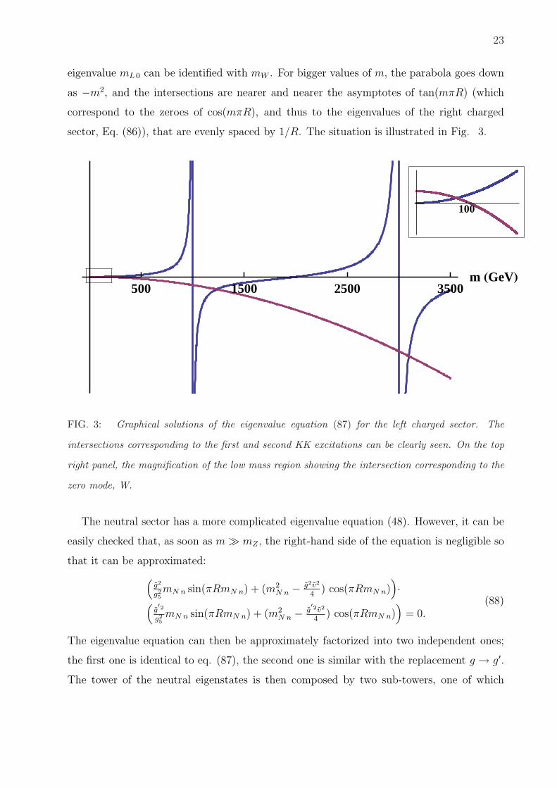
23

eigenvalue mL 0 can be identified with mW . For bigger values of m, the parabola goes down

as −m2, and the intersections are nearer and nearer the asymptotes of tan(mπR) (which

correspond to the zeroes of cos(mπR), and thus to the eigenvalues of the right charged

sector, Eq. (86)), that are evenly spaced by 1/R. The situation is illustrated in Fig. 3.

500 1500 2500 3500m HGeVL

100

FIG. 3: Graphical solutions of the eigenvalue equation (87) for the left charged sector. The

intersections corresponding to the first and second KK excitations can be clearly seen. On the top

right panel, the magnification of the low mass region showing the intersection corresponding to the

zero mode, W.

The neutral sector has a more complicated eigenvalue equation (48). However, it can be

easily checked that, as soon as m À mZ , the right-hand side of the equation is negligible so

that it can be approximated:

(g2

g25mN n sin(πRmN n) + (m2

N n − g2v2

4) cos(πRmN n)

)·

(g′2

g25mN n sin(πRmN n) + (m2

N n − g′2v2

4) cos(πRmN n)

)= 0.

(88)

The eigenvalue equation can then be approximately factorized into two independent ones;

the first one is identical to eq. (87), the second one is similar with the replacement g → g′.

The tower of the neutral eigenstates is then composed by two sub-towers, one of which

24

0 mode (GeV) 1st KK exc. (GeV) 2nd KK exc. (GeV)

Left charg. 80 1232 3096

Right charg. - 1000 3000

Neutral 0, 91 1056, 1232 3019, 3096

TABLE I: Low lying masses of the spectrum (zero modes and first two KK excitations) for the

model in the flat limit, with the following parameter choice: πR = 1.57 ·10−3 GeV−1, g5 = 1, naive

unitarity cut-off equal to 105 GeV.

almost identical to the one of the left sector. In Table I, we show the lightest part of the

spectrum in an explicit example corresponding to a particular choice of the parameters.

Let us now check the model against EW precision tests. In Fig. 4, we show the allowed

region at 95% C.L. in parameter space (M1, g5), based on the new physics contribution to

the ε parameters. Here M1 ≡ mR 1 = 1/2R is the mass of the lightest KK excitation, that is

of the first eigenstate of the right charged sector. The contour is obtained by a χ2 analysis,

based on the following experimental values for the ε parameters:

ε1 = (+5.4± 1.0)10−3

ε2 = (−8.9± 1.2)10−3

ε3 = (+5.34± 0.94)10−3

(89)

with correlation matrix

1 0.60 0.86

0.60 1 0.40

0.86 0.40 1

; (90)

(taken from [74]), and adding to the present model contribution the one from radiative

corrections in the SM. To fix the SM contribution, we set mt = 173.1 [75], α = 1/128.8

and consider two different test values of the Higgs mass, mH = 1 TeV and mH = 300 GeV.

Notice that, since we have considered SM fermion couplings, the new physics contribution

to εb is zero. Since the εb experimental value is very slightly correlated to ε1,2,3, we did not

25

100 TeV

50 TeV

20 TeV

500 1000 1500 2000

0.8

1.0

1.2

1.4

1.6

1.8

2.0

M1 HGeVL

g5

100 TeV

50 TeV

20 TeV

500 1000 1500 2000

0.8

1.0

1.2

1.4

1.6

1.8

2.0

M1 HGeVL

g5

FIG. 4: Allowed regions in the (M1, g5) parameter space for a flat extra dimension, for two values of

the Higgs mass: mH = 1 TeV (on the left) and mH = 300 GeV (on the right), based on electroweak

precision constraints. The corresponding naive unitarity cut-off is 105 GeV, so every shown state

is well within the unitarity limit. Also shown are the constraints from naive dimensional analysis

(contours correspond to different choices of the UV cut-off).

include this observable in the analysis. We get:

ε1 = 3.6 10−3, ε2 = −6.6 10−3, ε3 = 6.7 10−3, for mH = 1 TeV; (91)

ε1 = 4.8 10−3, ε2 = −7.1 10−3, ε3 = 6.1 10−3, for mH = 300 GeV; (92)

(these SM contributions are obtained as a linear interpolation from the values listed in [76]).

Fig. 4 also reports contours that correspond to several values of the naive unitarity cut-

off, (81). As it can be seen, the model is potentially compatible with EW precision data,

even for a relatively small mass scale for the new heavy vector states. Similarly to the SM

case a low Higgs mass is preferred. Even though a lighter Higgs mass seems to be preferred,

the limit it is not as stringent as in the SM: remember that, thanks to the decoupling, in the

limit M1 →∞ the SM picture is recovered, that is the region on the far right in Fig. 4 gives

the constraints in the SM case. The main drawback of the model in this limit is that since

it has a single extra dimension, which is compact, small and flat, it does not help solving

the hierarchy problem: the Higgs mass must still be adjusted through a fine-tuning exactly

as in the SM.

26

B. The model on a slice of AdS5

Probably, the most interesting case from the phenomenological point of view is that of

an exponentially warped extra-dimension, a slice of AdS5 space. This case corresponds to

choosing b(y) = e−2ky. The interest of this limit lies both in the possibility of solving the

hierarchy problem thanks to an exponential suppression of mass scales on the y = πR brane

(or IR brane where the Higgs is located) and in the AdS/CFT correspondence [7, 60, 61, 67],

according to which a model on AdS5 can be viewed as the dual description of a strongly

interacting model on four dimensions. In particular, in AdS/CFT fields localized near the IR

brane are interpreted as duals to composite states of the strong sector; in this interpretation

the Higgs field is no longer a fundamental field, but only an effective low-energy degree of

freedom, just like the KK excitations of the gauge fields.

With this choice we are in a sense come full circle, since we started my theoretical explo-

ration by considering the GD-BESS model, which gives a 4D low-energy effective description

of a strongly interacting sector; we generalized that model first to a moose one, then to a

5-dimensional one; finally, thanks to the AdS/CFT correspondence, we can read the gener-

alized 5D model again as an effective description of a strongly interacting theory.

The choice b(y) = e−2ky implies (again by eq. (62))

1

M2=

1

4k2

(e2kπR(2k2(πR)2 − 2kπR + 1)− 1

kπR

); (93)

the model has now an extra parameter, the curvature k, in addition to the usual πR, g5,

g, g′, v and λ. Eqs. (78), (79) and (80) still hold (with the new definition of M (93));

then, after fixing the standard EW input parameters, we are left with three free quantities,

πR and g5 and k. Then, if we want this model to be a potential solution to the hierarchy

problem, as the RS1 model [5], we need to fix the curvature parameter k to be around the

Planck scale, MP ' 1019 GeV. Then, to have M around one TeV, we need kπR ' 35.

Let’s look at the spectrum again. In this case, the C and S functions (eq. (45)) are given

by:

S(y, m) =eky

2kπ m

(J1

(mk

)Y1

(ekym

k

)− J1

(ekym

k

)Y1

(mk

))

C(y, m) =eky

2kπ m

(J1

(ekym

k

)Y0

(mk

)− J0

(mk

)Y1

(ekym

k

)),

(94)

where Ji and Yi are Bessel function of the first and of the second kind respectively. In this

case, not even the condition for the right charged eigenstates can be solved analytically.

27

0 mode (GeV) 1st KK exc. (GeV) 2nd KK exc. (GeV)

Left charg. 80 1316 16076

Right charg. - 1000 16054

Neutral 0, 91 1070, 1316 16058, 16076

TABLE II: Low lying masses of the spectrum (zero modes and first two KK excitations) for the

model in the RS limit, with the following parameter choice: k = 6.6 · 1018 GeV, kπR = 35, g5 = 1,

naive unitarity cut-off equal to 19 · 103 GeV.

0 mode (GeV) 1st KK exc. (GeV) 2nd KK exc. (GeV)

Left charg. 80 1307 8672

Right charg. - 1000 8632

Neutral 0, 91 1067, 1307 8640, 8672

TABLE III: Low lying masses of the spectrum (zero modes and first two KK excitations) for the

model in the RS limit, with the following parameter choice: k = 4.7 · 1018 GeV, kπR = 10, g5 = 1,

naive unitarity cut-off equal to 34 · 103 GeV.

However, using standard properties of the Bessel functions it is possible to give an estimate

for the first eigenvalue,

M1 ' k e−kπR 2√

2√4kπR− 3

, (95)

and for the characteristic spacing between two adjacent states, which is approximately con-

stant and equal to ∆M = πke−kπR. Notice that for kπR >> 1 the scale given by M is

nothing but M1.

The qualitative analysis made for the flat case generalizes almost verbatim to the AdS

case. The main difference is the typical distance between two adjacent eigenstates, which is

given by ∆M rather than simply by 1/R. In Tables II and III, we show examples of spectra

corresponding to particular choices of the model parameters. It is interesting to compare

this situation to the one of flat case; even though the masses of the first KK level in each

sector are roughly the same, the appearance of the second KK level is delayed to a much

higher scale.

28

50 TeV

15 TeV

5 TeV

500 1000 1500 2000

0.8

1.0

1.2

1.4

1.6

1.8

2.0

M1 HGeVL

g5

50 TeV

15 TeV

5 TeV

500 1000 1500 2000

0.8

1.0

1.2

1.4

1.6

1.8

2.0

M1 HGeVL

g5

FIG. 5: Allowed regions in the (M1, g5) parameter space for the model in the RS limit (b(y) = e−2ky,

with kπR fixed at 35), for two values of the Higgs mass: mH = 1 TeV (on the left) and mH = 300

GeV (on the right), based on electroweak precision constraints. Also shown are the constraints from

naive dimensional analysis (contours correspond to different choices of the UV cut-off).

Also in this case, we have checked the model against EW precision data using the ε

parameters. In Fig. 5, we show the allowed region at 95% C.L. in parameter space (M1, g5);

experimental data and SM radiative correction are the same of the flat case. The regions

slightly depend on the choice of kπR; here we have chosen kπR = 35; Fig. 5 also reports

contours that correspond to different values of the naive unitarity cut-off, (81) . Notice that

in this case, the UV cut-off due to unitarity is generally much lower than it was in the flat

case. Nevertheless, the model is again potentially compatible with EW precision data, even

when the new heavy vector states have masses around one TeV and an Higgs mass sensibly

greater than 100 − 200 GeV. The unitarity cut-off scale, which is quite low, calls for an

UV extension of the model at an energy scale which is not much higher than the potential

reach of the LHC; still the scenario described by the model seems interesting and deserves

an accurate study.

The physical content of the 5D D-BESS on an AdS background is very similar to the one of

the RS1-like model described in [20]. In that reference, the authors studied a SU(2)L⊗U(1)Y

5D gauge theory in AdS background, with localized kinetic terms on the IR brane. The main

difference between this set-up and the one we have outlined in this work is that we have

29

considered a larger SU(2)L ⊗ SU(2)R bulk gauge symmetry. Notice, however, that if we

add fermions in the simplest way, that is by localizing them on the IR brane (similarly

to what was done in refs. [38, 57]), then the extra gauge fields (that correspond to what

we called the “right charged sector”) are almost impossible to detect experimentally, since

they cannot interact with the fermions (by eq. (25) they have no superposition with the IR

brane). In fact, as can be seen by the effective Lagrangian calculation of section V, they

do not contribute to the ε parameters either. In conclusion, even if the bulk gauge group

is different, the phenomenology of the two models is almost identical (the situation change,

however, if fermions are allowed to propagate in the bulk).

This is a very interesting conclusion: working with a completely bottom-up approach,

starting from an effective 4D theory - the GD-BESS model - and generalizing, we have

arrived at a 5D model that quite closely reproduces a particular version of RS1.

VII. CONCLUSIONS

Acknowledgments

The authors would like to thank R. Contino and M. Redi for stimulating discussions and

V. Ciulli for clarifying comments on statistical analysis.

30

APPENDIX A: DERIVATION OF THE CONDITIONS FOR THE KK

EXPANSION

We will now show how eqs. from (14) to (32) can be derived from the request that the

effective 4D Lagrangian is diagonal. Throughout the following calculation, we will only need

to work with the bilinear gauge part of the action (8). Expanding the gauge fields as in

eq. (13) without assuming anything a priori on the form of the functions faj and ga

j and the

constants caj and carrying out the integration with respect to the extra dimension, we get

L(2) = −1

4V (j)

µν V (k) µνAjk − 1

2V (j)

µ V (k) µBjk

−1

2∂µG

(j)∂µG(k)Cjk + V (j)µ ∂µG(k)Djk,

(A1)

where we defined the matrices:

Ajk =1

g25

∫ πR

0

dy(fa

L jfaL k + fa

R jfaR k

)+

1

g2fa

L jfaL k

∣∣πR

+1

g′2f 3

R jf3R k

∣∣πR

;

Bjk =1

g25

∫ πR

0

dy b(y)(∂yf

aL j∂yf

aL k + ∂yf

aR j∂yf

aR k

)

+v2

4b(πR)

(fa

L jfaL k + f 3

R jf3R k − 2f 3

L jf3R k

) ∣∣πR

;

Cjk =1

g25

∫ πR

0

dy b(y)(ga

L jgaL k + ga

R jgaR k

)+ ca

j cak;

Djk =1

g25

∫ πR

0

dy b(y)∂y

(fa

L jgaL k + fa

R jgaR k

)

− v

2

(fa

L jcak − f 3

R jc3k

)∣∣πR

.

(A2)

In the expanded Lagrangian (A1), it is possible to recognize vector and scalar kinetic-like

terms, vector mass-like terms and vector / would-be goldstone mixings. However, all those

terms are in general not diagonal with respect to the KK number. This is of course a direct

consequence of the general nature of the expansion (13). However, if the expanded theory is

to be consistent, it must be possible to obtain the actual physical degrees of freedom - with

explicitly diagonal mass and kinetic terms - by defining appropriate linear combinations of

the modes V(j)µ and G(j). We then introduce a still general basis change in field space:

V (j)µ = Rjk V (k)

µ ; G(j) = Sjk G(k), (A3)

31

and require the Lagrangian (A1) to be diagonal in terms of the new degrees of freedom V(j)µ

and G(j). This means that the matrices RT AR, RT BR, ST CS and RT DS (all the fields are

real, so we can choose the matrices R and S to be orthogonal) have to be diagonal. Since in

general it is not possible to diagonalize four independent matrices using just two rotations,

we will need to impose a set of consistency conditions on the wave-functions faL,R j and ga

L,R j

and the constants caj , that will determine the wave functions uniquely.

Let’s define:

faL,R j = Rjk fa

L,R k; gaL,R j = Sjk ga

L,R k, caj = Sjk ca

k; (A4)

the conditions that we need to impose on the KK modes are then:

1

g25

∫ πR

0

dy(fa

L j faL k + fa

R j faR k

)+

1

g2fa

L j faL k

∣∣πR

+1

g′2f 3

R j f3R k

∣∣πR

= ajδjk;

(A5a)

1

g25

∫ πR

0

dy b(y)(∂yf

aL j∂yf

aL k + ∂yf

aR j∂yf

aR k

)

+v2

4b(πR)

(fa

L j faL k + f 3

R j f3R k − 2f 3

L j f3R k

) ∣∣πR

= bjδjk;

(A5b)

1

g25

∫ πR

0

dy b(y)(ga

L j gaL k + ga

R j gaR k

)+ ca

j cak = cjδjk; (A5c)

1

g25

∫ πR

0

dy b(y)(∂yf

aL j g

aL k + ∂yf

aR j g

aR k

)

− v

2

(fa

L j cak − f 3

R j c3k

)∣∣∣πR

= djδjk.

(A5d)

We want to reduce the set of eqs. (A5) to a more explicit form. As a first thing, consider

the integral appearing in the left-hand side of eq. (A5b). It can be rewritten∫ πR

0

b(y) ∂yfaL j∂yf

aL k dy + (L → R)

= −∫ πR

0

faL j∂y(b(y) ∂yf

aL k) dy + b(πR) fa

L j∂yfaL k

∣∣πR

0+ (L → R).

(A6)

If the eigenfunctions faL,R j satisfy the equation of motion:

DfaL,R j = −m2

jfaL,R j, (A7)

where we leave the eigenvalue mj for now unspecified, then the integral in eq. (A6) can be

further simplified to

−m2k

∫ πR

0

faL j f

aL k dy + b(πR) fa

L j∂yfaL k

∣∣πR

0+ (L → R). (A8)

32

Now notice from eqs. (A5) that the left and right wave-functions only mix through their

3rd isospin components. So the conditions (A5) receive three separate contributions, one

from left wave-functions with isospin a = 1, 2, another from a = 1, 2 right wave-functions

and the last one from mixed left/right a = 3 modes. The simplest, most natural choice is

to diagonalize the three contributions independently. In this way, we will get three different

sets of BCs, that is three decoupled towers of mass eigenstates. While this may not be the

most general solution to eqs. (A5), it is consistent with the symmetry breaking pattern.

The general expansion (13) can then be recast into a more explicit form:

W 1,2L µ(x, y) =

∞∑n=0

f 1,2L n(y) W

1,2 (n)L µ (x), W 1,2

L 5(x, y) =∞∑

n=0

g1,2L n(y) G

1,2 (n)L (x),

W 1,2R µ(x, y) =

∞∑n=0

f 1,2R n(y) W

1,2 (n)R µ (x), W 1,2

R 5(x, y) =∞∑

n=0

g1,2R n(y) G

1,2 (n)R (x),

W 3L µ(x, y) =

∞∑n=0

f 3L n(y) N (n)

µ (x), W 3L 5(x, y) =

∞∑n=0

g3L n(y) G

(n)N (x),

W 3R µ(x, y) =

∞∑n=0

f 3R n(y) N (n)

µ (x), W 3R 5(x, y) =

∞∑n=0

g3R n(y) G

(n)N (x),

π1,2(x) =∞∑

n=0

c1,2n G(n)(x), π3(x) =

∞∑n=0

c3n G(n)(x).

(A9)

As a consequence of this redefinition, the equation of motion (A7) can also be more explicitly

rewritten as three separate equations:

Df 1,2L n = −m2

L nf1,2L n, (A10)

Df 1,2R n = −m2

R nf 1,2R n, (A11)

Df 3L,R n = −m2

N nf3L,R n, (A12)

to emphasize the fact that to each sector corresponds a different set of eigenvalues. These

three equations reproduce precisely eq. (15), (23) and (29).

To go on, assume that the wave-functions obey orthogonality conditions:

(faL m, fa

L n)g = δmn,1

g25

(f 1,2R m, f 1,2

R n)L2 = δmn, (f 3R m, f 3

R n)g′ = δmn, (A13)

where the (·, ·)g scalar product was defined in eq. (20). With this assumption, the left-hand

side of eq. (A5a) becomes diagonal, and the equation itself is satisfied by choosing an ≡ 1.

33

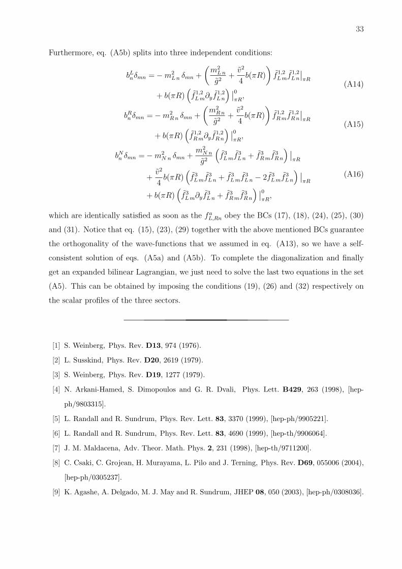
Furthermore, eq. (A5b) splits into three independent conditions:

bLnδmn =−m2

L n δmn +

(m2

L n

g2+

v2

4b(πR)

)f 1,2

L mf 1,2L n

∣∣πR

+ b(πR)(f 1,2

L m∂yf1,2L n

) ∣∣0πR

,

(A14)

bRn δmn =−m2

R n δmn +

(m2

R n

g2+

v2

4b(πR)

)f 1,2

R mf 1,2R n

∣∣πR

+ b(πR)(f 1,2

R m∂yf1,2R n

) ∣∣0πR

,

(A15)

bNn δmn =−m2

N n δmn +m2

N n

g2

(f 3

L mf 3L n + f 3

R mf 3R n

) ∣∣πR

+v2

4b(πR)

(f 3

L mf 3L n + f 3

L mf 3L n − 2f 3

L mf 3L n

) ∣∣πR

+ b(πR)(f 3

L m∂yf3L n + f 3

R mf 3R n

) ∣∣0πR

,

(A16)

which are identically satisfied as soon as the faL,Rn obey the BCs (17), (18), (24), (25), (30)

and (31). Notice that eq. (15), (23), (29) together with the above mentioned BCs guarantee

the orthogonality of the wave-functions that we assumed in eq. (A13), so we have a self-

consistent solution of eqs. (A5a) and (A5b). To complete the diagonalization and finally

get an expanded bilinear Lagrangian, we just need to solve the last two equations in the set

(A5). This can be obtained by imposing the conditions (19), (26) and (32) respectively on

the scalar profiles of the three sectors.

[1] S. Weinberg, Phys. Rev. D13, 974 (1976).

[2] L. Susskind, Phys. Rev. D20, 2619 (1979).

[3] S. Weinberg, Phys. Rev. D19, 1277 (1979).

[4] N. Arkani-Hamed, S. Dimopoulos and G. R. Dvali, Phys. Lett. B429, 263 (1998), [hep-

ph/9803315].

[5] L. Randall and R. Sundrum, Phys. Rev. Lett. 83, 3370 (1999), [hep-ph/9905221].

[6] L. Randall and R. Sundrum, Phys. Rev. Lett. 83, 4690 (1999), [hep-th/9906064].

[7] J. M. Maldacena, Adv. Theor. Math. Phys. 2, 231 (1998), [hep-th/9711200].

[8] C. Csaki, C. Grojean, H. Murayama, L. Pilo and J. Terning, Phys. Rev. D69, 055006 (2004),

[hep-ph/0305237].

[9] K. Agashe, A. Delgado, M. J. May and R. Sundrum, JHEP 08, 050 (2003), [hep-ph/0308036].

34

[10] C. Csaki, C. Grojean, L. Pilo and J. Terning, Phys. Rev. Lett. 92, 101802 (2004), [hep-

ph/0308038].

[11] G. Cacciapaglia, C. Csaki, C. Grojean and J. Terning, ECONF C040802, FRT004 (2004).

[12] G. Cacciapaglia, C. Csaki, C. Grojean and J. Terning, Phys. Rev. D71, 035015 (2005),

[hep-ph/0409126].

[13] G. Cacciapaglia, C. Csaki, C. Grojean and J. Terning, Phys. Rev. D70, 075014 (2004),

[hep-ph/0401160].

[14] R. Contino, T. Kramer, M. Son and R. Sundrum, JHEP 05, 074 (2007), [hep-ph/0612180].

[15] H. Davoudiasl, J. L. Hewett, B. Lillie and T. G. Rizzo, JHEP 05, 015 (2004), [hep-ph/0403300].

[16] G. Cacciapaglia, C. Csaki, G. Marandella and J. Terning, JHEP 02, 036 (2007), [hep-

ph/0611358].

[17] M. S. Carena, E. Ponton, J. Santiago and C. E. M. Wagner, Nucl. Phys. B759, 202 (2006),

[hep-ph/0607106].

[18] M. S. Carena, T. M. P. Tait and C. E. M. Wagner, Acta Phys. Polon. B33, 2355 (2002),

[hep-ph/0207056].

[19] C. Csaki, J. Erlich and J. Terning, Phys. Rev. D66, 064021 (2002), [hep-ph/0203034].

[20] M. S. Carena, E. Ponton, T. M. P. Tait and C. E. M. Wagner, Phys. Rev. D67, 096006 (2003),

[hep-ph/0212307].

[21] Y. Cui, T. Gherghetta and J. D. Wells, JHEP 11, 080 (2009), [0907.0906].

[22] R. Foadi and C. Schmidt, Phys. Rev. D73, 075011 (2006), [hep-ph/0509071].

[23] R. Casalbuoni, S. De Curtis, D. Dominici and D. Dolce, JHEP 08, 053 (2007),

[arXiv:0705.2510 [hep-ph]].

[24] Y. Nomura, JHEP 11, 050 (2003), [hep-ph/0309189].

[25] R. Barbieri, A. Pomarol and R. Rattazzi, Phys. Lett. B591, 141 (2004), [hep-ph/0310285].

[26] R. Barbieri, A. Pomarol, R. Rattazzi and A. Strumia, Nucl. Phys. B703, 127 (2004), [hep-

ph/0405040].

[27] N. Arkani-Hamed, A. G. Cohen and H. Georgi, Phys. Rev. Lett. 86, 4757 (2001), [hep-

th/0104005].

[28] N. Arkani-Hamed, A. G. Cohen and H. Georgi, Phys. Lett. B513, 232 (2001), [hep-

ph/0105239].

[29] C. T. Hill, S. Pokorski and J. Wang, Phys. Rev. D64, 105005 (2001), [hep-th/0104035].

35

[30] H.-C. Cheng, C. T. Hill, S. Pokorski and J. Wang, Phys. Rev. D64, 065007 (2001), [hep-

th/0104179].

[31] H. Abe, T. Kobayashi, N. Maru and K. Yoshioka, Phys. Rev. D67, 045019 (2003), [hep-

ph/0205344].

[32] A. Falkowski and H. D. Kim, JHEP 08, 052 (2002), [hep-ph/0208058].

[33] L. Randall, Y. Shadmi and N. Weiner, JHEP 01, 055 (2003), [hep-th/0208120].

[34] D. T. Son and M. A. Stephanov, Phys. Rev. D69, 065020 (2004), [hep-ph/0304182].

[35] J. de Blas, A. Falkowski, M. Perez-Victoria and S. Pokorski, JHEP 08, 061 (2006), [hep-

th/0605150].

[36] R. Foadi, S. Gopalakrishna and C. Schmidt, JHEP 03, 042 (2004), [hep-ph/0312324].

[37] J. Hirn and J. Stern, Eur. Phys. J. C34, 447 (2004), [hep-ph/0401032].

[38] R. Casalbuoni, S. De Curtis and D. Dominici, Phys. Rev. D70, 055010 (2004), [hep-

ph/0405188].

[39] R. S. Chivukula, E. H. Simmons, H.-J. He, M. Kurachi and M. Tanabashi, Phys. Rev. D70,

075008 (2004), [hep-ph/0406077].

[40] H. Georgi, Phys. Rev. D71, 015016 (2005), [hep-ph/0408067].

[41] J. Bechi, R. Casalbuoni, S. De Curtis and D. Dominici, Phys. Rev. D74, 095002 (2006),

[hep-ph/0607314].

[42] R. Foadi, S. Gopalakrishna and C. Schmidt, Phys. Lett. B606, 157 (2005), [hep-ph/0409266].

[43] R. Casalbuoni, S. De Curtis, D. Dolce and D. Dominici, Phys. Rev. D71, 075015 (2005),

[hep-ph/0502209].

[44] B. Coleppa, S. Di Chiara and R. Foadi, JHEP 05, 015 (2007), [hep-ph/0612213].

[45] D. Becciolini, M. Redi and A. Wulzer, 0906.4562.

[46] R. Casalbuoni, S. De Curtis, D. Dominici and R. Gatto, Phys. Lett. B155, 95 (1985).

[47] R. Casalbuoni, S. De Curtis, D. Dominici and R. Gatto, Nucl. Phys. B282, 235 (1987).

[48] R. S. Chivukula et al., Phys. Rev. D74, 075011 (2006), [hep-ph/0607124].

[49] S. Matsuzaki, R. S. Chivukula, E. H. Simmons and M. Tanabashi, Phys. Rev. D75, 073002

(2007), [hep-ph/0607191].

[50] S. Matsuzaki, R. S. Chivukula, E. H. Simmons and M. Tanabashi.

[51] S. Dawson and C. B. Jackson, Phys. Rev. D76, 015014 (2007), [hep-ph/0703299].

[52] T. Abe, S. Matsuzaki and M. Tanabashi, Phys. Rev. D78, 055020 (2008), [0807.2298].

36

[53] M. E. Peskin and T. Takeuchi, Phys. Rev. Lett. 65, 964 (1990).

[54] M. E. Peskin and T. Takeuchi, Phys. Rev. D46, 381 (1992).

[55] R. Casalbuoni et al., Phys. Lett. B349, 533 (1995), [hep-ph/9502247].

[56] R. Casalbuoni et al., Phys. Rev. D53, 5201 (1996), [hep-ph/9510431].

[57] R. Casalbuoni, F. Coradeschi, S. De Curtis and D. Dominici, Phys. Rev. D77, 095005 (2008),

[0710.3057].

[58] T. Appelquist and C. W. Bernard, Phys. Rev. D22, 200 (1980).

[59] A. C. Longhitano, Phys. Rev. D22, 1166 (1980).

[60] N. Arkani-Hamed, M. Porrati and L. Randall, JHEP 08, 017 (2001), [hep-th/0012148].

[61] R. Rattazzi and A. Zaffaroni, JHEP 04, 021 (2001), [hep-th/0012248].

[62] A. Falkowski, Phys. Rev. D75, 025017 (2007), [hep-ph/0610336].

[63] A. Falkowski, S. Pokorski and J. P. Roberts, JHEP 12, 063 (2007), [0705.4653].

[64] G. Altarelli and R. Barbieri, Phys. Lett. B253, 161 (1991).

[65] G. Altarelli, R. Barbieri and S. Jadach, Nucl. Phys. B369, 3 (1992).

[66] G. Altarelli, R. Barbieri and F. Caravaglios, Nucl. Phys. B405, 3 (1993).

[67] E. Witten, Adv. Theor. Math. Phys. 2, 253 (1998), [hep-th/9802150].

[68] M. Perez-Victoria, JHEP 05, 064 (2001), [hep-th/0105048].

[69] G. Burdman and Y. Nomura, Phys. Rev. D69, 115013 (2004), [hep-ph/0312247].

[70] M. A. Luty, M. Porrati and R. Rattazzi, JHEP 09, 029 (2003), [hep-th/0303116].

[71] A. Delgado and A. Falkowski, JHEP 05, 097 (2007), [hep-ph/0702234].

[72] R. Sekhar Chivukula, D. A. Dicus and H.-J. He, Phys. Lett. B525, 175 (2002), [hep-

ph/0111016].

[73] R. Casalbuoni, S. De Curtis, D. Dominici and M. Grazzini, Phys. Rev. D56, 5731 (1997),

[hep-ph/9704229].

[74] ALEPH, Phys. Rept. 427, 257 (2006), [hep-ex/0509008].

[75] Tevatron Electroweak Working Group, 0903.2503.

[76] G. Altarelli, Lectures given at Zuoz Summer School on Phenomenology of Gauge Interactions,

13-19 Aug 2000 , [hep-ph/0011078].