56:171 Fall 2002 Operations Research Homework Solutionsuser.engineering.uiowa.edu/~dbricker/OR_Sample_HW/OR_HW_F02_… · Fall 2002 Operations Research Homework Solutions ... Dept.

56:171

Fall 2002

Operations Research

Homework Solutions Instructor: D. L. Bricker

University of Iowa

Dept. of Mechanical & Industrial Engineering

56:171 O.R. -- HW #1 Solution Fall 2001 page 1 of 5

56:171 Operations ResearchHomework #1 Solutions –Fall 2002

1. The Keyesport Quarry has two different pits from which it obtains rock. The rock is run through acrusher to produce two products: concrete grade stone and road surface chat. Each ton of rock fromthe South pit converts into 0.75 tons of stone and 0.25 tons of chat when crushed. Rock from theNorth pit is of different quality. When it is crushed it produces a “50-50” split of stone and chat. TheQuarry has contracts for 60 tons of stone and 40 tons of chat this planning period. The cost per ton ofextracting and crushing rock from the South pit is 1.6 times as costly as from the North pit.

a. What are the decision variables in the problem? Be sure to give their definitions, not just theirnames!Answer: S_ROCK = # of tons of rocks from the South pit.

N_ROCK = # of tons of rocks from the North pit.

b. There are two constraints for this problem. • State them in words.Answer:1. # of tons of concrete grade stone which is the sum of concrete grade stone from South pit and

concrete grade stone from North pit is bigger than 60.2. # of tons of road surface chat which is the sum of road surface chat from South pit and road

surface chat from North pit is bigger than 40.• State them in equation or inequality form.Answer:

0.75 S_ROCK + 0.5 N_ROCK ≥ 600.25 S_ROCK + 0.5 N_ROCK ≥ 40

c. State the objective function.Answer:

Total cost of the processing rocks which is the sum of the cost of processing rocks fromSouth pit and North pit in the unit of the cost of processing 1 ton’s processing North pit(to be minimized):

Min 1.6 S_ROCK + N_ROCK

d. Graph the feasible region (in 2 dimensions) for this problem.


Answer:

e. Draw an appropriate objective function line on the graph and indicate graphically and numericallythe optimal solution.Answer:

f. Use LINDO (or other appropriate LP solver) to compute the optimal solution.


Answer:

LP OPTIMUM FOUND AT STEP 1

OBJECTIVE FUNCTION VALUE

1) 120.0000

VARIABLE VALUE REDUCED COSTS_ROCK 0.000000 0.100000N_ROCK 120.000000 0.000000

ROW SLACK OR SURPLUS DUAL PRICES2) 0.000000 -2.0000003) 20.000000 0.000000

◆ ◆ ◆ ◆ ◆ ◆ ◆ ◆ ◆ ◆ ◆ ◆ ◆ ◆

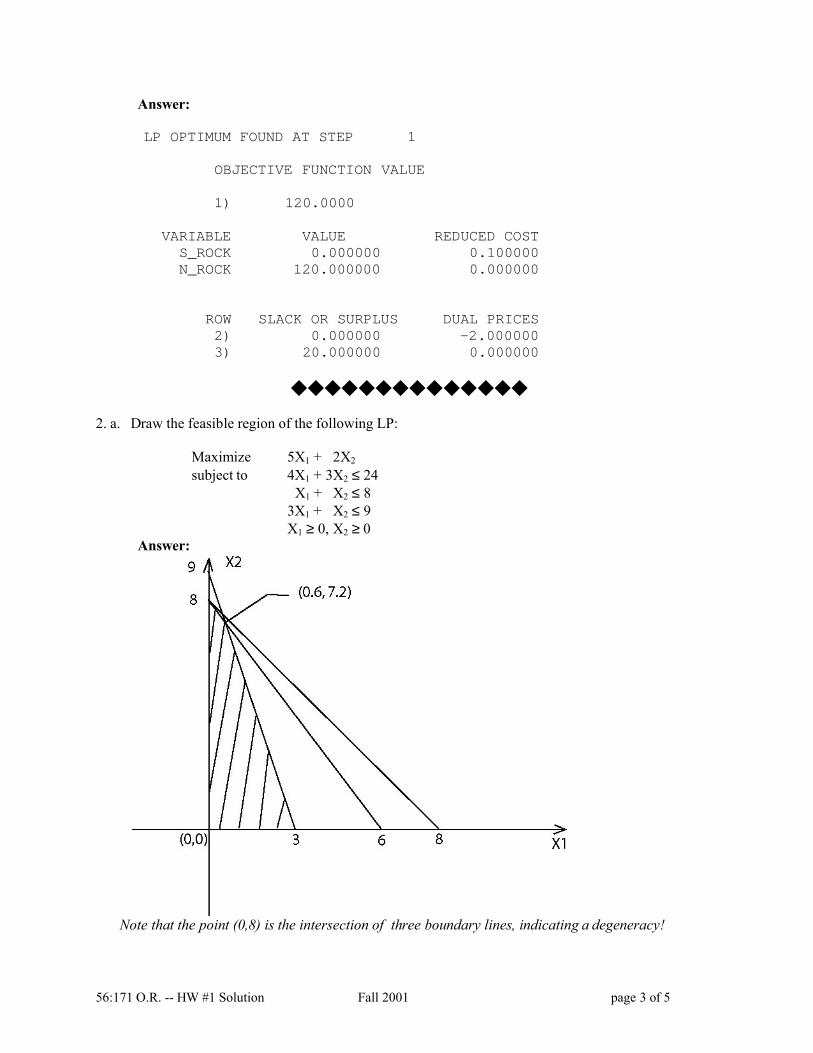
2. a. Draw the feasible region of the following LP:

Maximize 5X1 + 2X2

subject to 4X1 + 3X2 ≤ 24X1 + X2 ≤ 8

3X1 + X2 ≤ 9X1 ≥ 0, X2 ≥ 0

Answer:

Note that the point (0,8) is the intersection of three boundary lines, indicating a degeneracy!


b. Indicate on the graph the optimal solution.Answer:

◆ ◆ ◆ ◆ ◆ ◆ ◆ ◆ ◆ ◆ ◆ ◆ ◆ ◆

3. a. Compute the inverse of the matrix (showing your computational steps):

1 0 11 2 02 1 1

A−

= − −

Answer:1 0 1 1 0 01 2 0 0 1 02 1 0 0 0 1

− − −

2 2 1 2 2

3 3 1 3 3 2

1 0 1 1 0 0 / 22 0 2 1 1 1 0 / 2

~ 0 1 1 2 0 1 ~

R R R R RR R R R R R

= − − = = + − = + − −

1 1 3

2 2 3

3 3

21 0 1 1 0 0 1 0 0 2 1 20 1 1/ 2 1/ 2 1/ 2 0 0 1 0 1 1 1

20 0 1/ 2 3/ 2 1/ 2 1 0 0 1 3 1 2

~

R R RR R RR R

= −− − − −

= + − = − − − − −


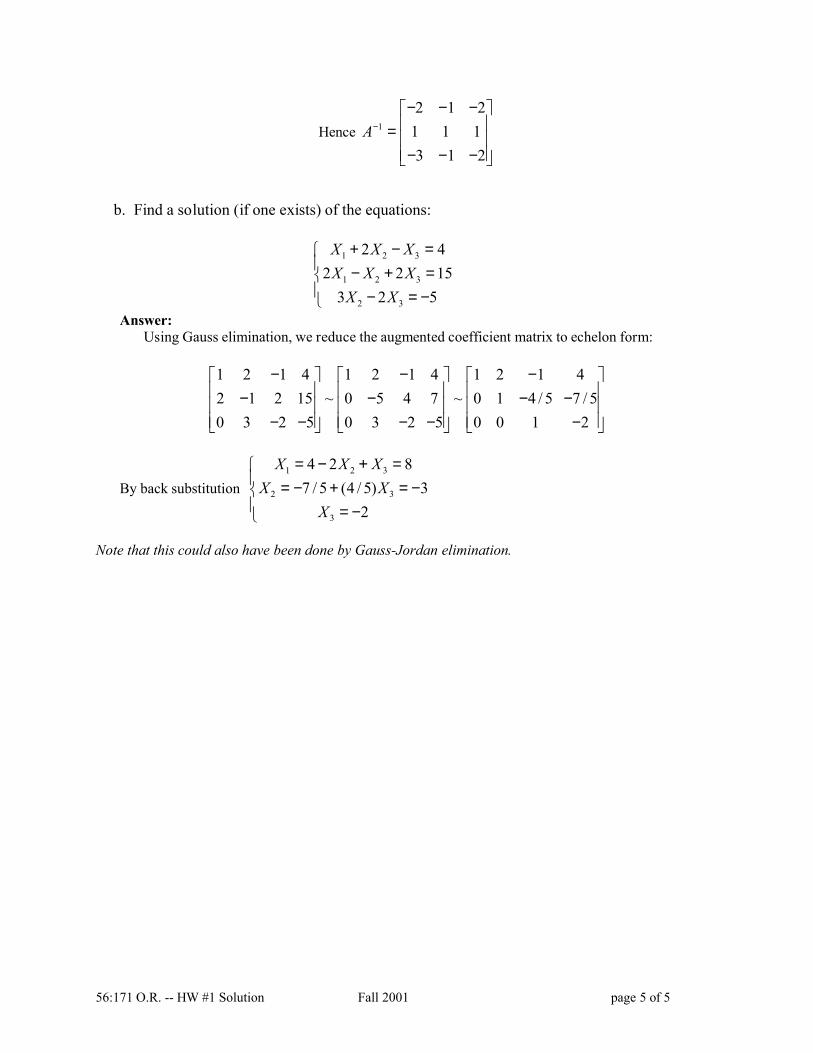
Hence 1

2 1 21 1 13 1 2

A−

− − − = − − −

b. Find a solution (if one exists) of the equations:

1 2 3

1 2 3

2 3

2 42 2 15

3 2 5

X X XX X X

X X

+ − = − + = − = −

Answer:Using Gauss elimination, we reduce the augmented coefficient matrix to echelon form:

1 2 1 4 1 2 1 4 1 2 1 42 1 2 15 ~ 0 5 4 7 ~ 0 1 4 / 5 7 / 50 3 2 5 0 3 2 5 0 0 1 2

− − − − − − − − − − − −

By back substitution 1 2 3

2 3

3

4 2 87 / 5 (4 / 5) 3

2

X X XX X

X

= − + = = − + = − = −

Note that this could also have been done by Gauss-Jordan elimination.

56:171 O.R. -- HW #2 Solution Fall 2001 page 1

56:171 Operations ResearchHomework #2 Solutions – Fall 2002

1. (Exercise 3.4-18, page 98, of Hillier&Lieberman text, 7th edition)“Oxbridge University maintains a powerful mainframe computer for research use

by its faculty, Ph.D. students, and research associates. During all working hours, anoperator must be able to operate and maintain the computer, as well as to performsome programming services. Beryl Ingram, the director of the computer facility,oversees the operation.

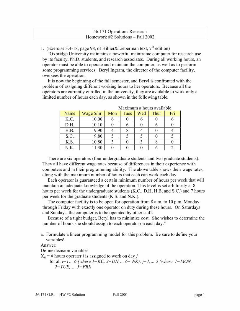
It is now the beginning of the fall semester, and Beryl is confronted with theproblem of assigning different working hours to her operators. Because all theoperators are currently enrolled in the university, they are available to work only alimited number of hours each day, as shown in the following table.

Maximum # hours availableName Wage $/hr Mon Tues Wed Thur FriK.C. 10.00 6 0 6 0 6D.H. 10.10 0 6 0 6 0H.B. 9.90 4 8 4 0 4S.C. 9.80 5 5 5 0 5K.S. 10.80 3 0 3 8 0N.K. 11.30 0 0 0 6 2

There are six operators (four undergraduate students and two graduate students). They all have different wage rates because of differences in their experience withcomputers and in their programming ability. The above table shows their wage rates,along with the maximum number of hours that each can work each day.

Each operator is guaranteed a certain minimum number of hours per week that willmaintain an adequate knowledge of the operation. This level is set arbitrarily at 8hours per week for the undergraduate students (K.C,, D.H, H.B, and S.C.) and 7 hoursper week for the graduate students (K.S. and N.K.).

The computer facility is to be open for operation from 8 a.m. to 10 p.m. Mondaythrough Friday with exactly one operator on duty during these hours. On Saturdaysand Sundays, the computer is to be operated by other staff.

Because of a tight budget, Beryl has to minimize cost. She wishes to determine thenumber of hours she should assign to each operator on each day.”

a. Formulate a linear programming model for this problem. Be sure to define yourvariables!

Answer:Define decision variablesXij = # hours operater i is assigned to work on day j

for all i=1… 6 (where 1=KC, 2=DH,… 6= NK); j=1,… 5 (where 1=MON,2=TUE, … 5=FRI)


Minimize z= 10(X11 + X13 + X15) + 10.1(X22 + X24) + 9.9(X31 + X32 + X33+X35) +9.8(X41 + X42 + X43 + X45) + 10.8(X51 + X53 + X54) + 11.3(X64 + X65)

subject tomaximum number hours available each day:X11≤6 X22≤6 X31≤4 X41≤5 X51≤3 X64≤6X13≤6 X24≤6 X32≤8 X42≤5 X53≤3 X65≤2X15≤6 X33≤4 X43≤5 X54≤8

X35≤4 X45≤5number of hours guaranteed for each operator:X11 + X13 + X15 ≥ 8 X41 + X42 + X43 + X45 ≥ 8X22 + X24 ≥ 8 X51 + X53 + X54 ≥ 7X31 + X32 + X33 + X35 ≥ 8 X64 + X65 ≥ 7

total number hours worked each day is 14:X11 + X31 + X41 + X51 = 14 X24 + X44 + X54 + X64 = 14X22 + X23 + X42 = 14 X15 + X35 + X45 + X65 = 14X13 + X33 + X43 + X53 = 14

nonnegativity:Xij ≥ 0 for all i & j

b. Use an LP solver (e.g. LINDO or LINGO) to find the optimal solution.

The LINGO model is as follows:MODEL: ! Oxbridge University Computer Center;

SETS:OPERATOR / KC, DH, HB, SC, KS, NK/: MINIMUM, PAYRATE;DAY /MON, TUE, WED, THU, FRI/: REQUIRED;ASSIGN(OPERATOR,DAY): AVAILABLE, X;

ENDSETS

DATA:MINIMUM = 8 8 8 8 7 7;PAYRATE = 10.00 10.10 9.90 9.80 10.80 11.30;REQUIRED = 14 14 14 14 14;AVAILABLE= 6 0 6 0 6

0 6 0 6 04 8 4 0 45 5 5 0 53 0 3 8 00 0 0 6 2;

ENDDATA

MIN = TOTALPAY;

! total weekly payroll cost;TOTALPAY = @SUM(ASSIGN(I,J)|AVAILABLE(I,J) #NE# 0:

PAYRATE(I)*X(I,J) );


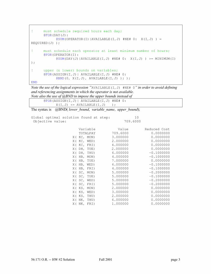
! must schedule required hours each day;@FOR(DAY(J):

@SUM(OPERATOR(I)|AVAILABLE(I,J) #NE# 0: X(I,J) ) =REQUIRED(J) );

! must schedule each operator at least minimum number of hours;@FOR(OPERATOR(I):

@SUM(DAY(J)|AVAILABLE(I,J) #NE# 0: X(I,J) ) >= MINIMUM(I));

! upper (& lower) bounds on variables;@FOR(ASSIGN(I,J)| AVAILABLE(I,J) #NE# 0:

@BND(0, X(I,J), AVAILABLE(I,J) ); );END

Note the use of the logical expression “AVAILABLE(I,J) #NE# 0” in order to avoid definingand referencing assignments in which the operator is not available.Note also the use of @BND to impose the upper bounds instead of

@FOR(ASSIGN(I,J)| AVAILABLE(I,J) #NE# 0:X(I,J) <= AVAILABLE(I,J) );

The syntax is @BND( lower_bound, variable_name, upper_bound);

Global optimal solution found at step: 10Objective value: 709.6000

Variable Value Reduced CostTOTALPAY 709.6000 0.0000000

X( KC, MON) 3.000000 0.0000000X( KC, WED) 2.000000 0.0000000X( KC, FRI) 4.000000 0.0000000X( DH, TUE) 2.000000 0.0000000X( DH, THU) 6.000000 -0.1000000X( HB, MON) 4.000000 -0.1000000X( HB, TUE) 7.000000 0.0000000X( HB, WED) 4.000000 -0.1000000X( HB, FRI) 4.000000 -0.1000000X( SC, MON) 5.000000 -0.2000000X( SC, TUE) 5.000000 -0.1000000X( SC, WED) 5.000000 -0.2000000X( SC, FRI) 5.000000 -0.2000000X( KS, MON) 2.000000 0.0000000X( KS, WED) 3.000000 0.0000000X( KS, THU) 2.000000 0.0000000X( NK, THU) 6.000000 0.0000000X( NK, FRI) 1.000000 0.0000000


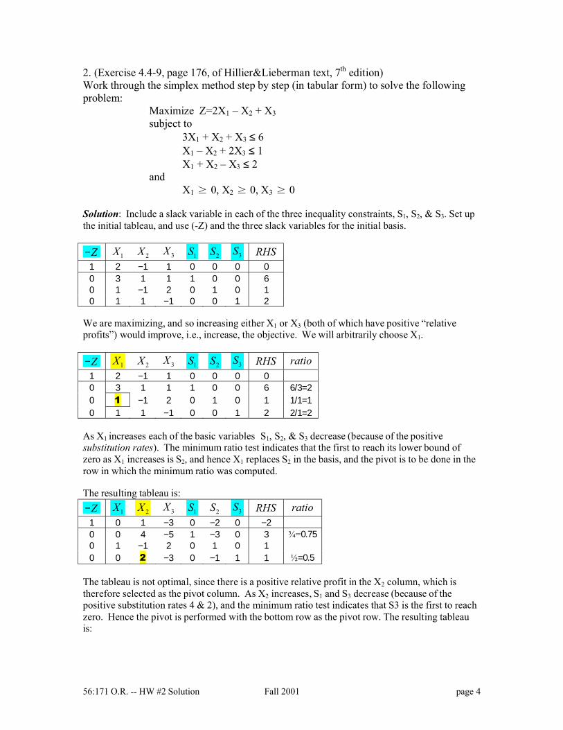
2. (Exercise 4.4-9, page 176, of Hillier&Lieberman text, 7th edition)Work through the simplex method step by step (in tabular form) to solve the followingproblem:

Maximize Z=2X1 – X2 + X3subject to

3X1 + X2 + X3 ≤ 6X1 – X2 + 2X3 ≤ 1X1 + X2 – X3 ≤ 2

andX1 ≥ 0, X2 ≥ 0, X3 ≥ 0

Solution: Include a slack variable in each of the three inequality constraints, S1, S2, & S3. Set upthe initial tableau, and use (-Z) and the three slack variables for the initial basis.

Z− 1X 2X 3X 1S 2S 3S RHS1 2 −1 1 0 0 0 0 0 3 1 1 1 0 0 6 0 1 −1 2 0 1 0 1 0 1 1 −1 0 0 1 2

We are maximizing, and so increasing either X1 or X3 (both of which have positive “relativeprofits”) would improve, i.e., increase, the objective. We will arbitrarily choose X1.

Z− 1X 2X 3X 1S 2S 3S RHS ratio1 2 −1 1 0 0 0 0 0 3 1 1 1 0 0 6 6/3=2 0 1 −1 2 0 1 0 1 1/1=1 0 1 1 −1 0 0 1 2 2/1=2

As X1 increases each of the basic variables S1, S2, & S3 decrease (because of the positivesubstitution rates). The minimum ratio test indicates that the first to reach its lower bound ofzero as X1 increases is S2, and hence X1 replaces S2 in the basis, and the pivot is to be done in therow in which the minimum ratio was computed.

The resulting tableau is:Z− 1X 2X 3X 1S 2S 3S RHS ratio1 0 1 −3 0 −2 0 −2 0 0 4 −5 1 −3 0 3 ¾=0.75 0 1 −1 2 0 1 0 1 0 0 2 −3 0 −1 1 1 ½=0.5

The tableau is not optimal, since there is a positive relative profit in the X2 column, which istherefore selected as the pivot column. As X2 increases, S1 and S3 decrease (because of thepositive substitution rates 4 & 2), and the minimum ratio test indicates that S3 is the first to reachzero. Hence the pivot is performed with the bottom row as the pivot row. The resulting tableauis:


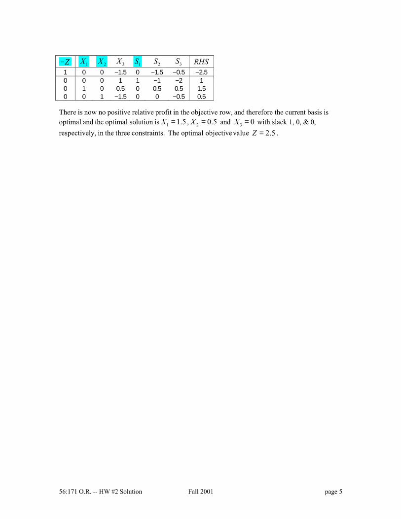
Z− 1X 2X 3X 1S 2S 3S RHS1 0 0 −1.5 0 −1.5 −0.5 −2.5 0 0 0 1 1 −1 −2 1 0 1 0 0.5 0 0.5 0.5 1.5 0 0 1 −1.5 0 0 −0.5 0.5

There is now no positive relative profit in the objective row, and therefore the current basis isoptimal and the optimal solution is 1 1.5X = , 2 0.5X = and 3 0X = with slack 1, 0, & 0,respectively, in the three constraints. The optimal objective value 2.5Z = .

Solutions

56:171 O.R. -- HW #3 Solutions Fall 2002 page 1 of 8

56:171 Operations ResearchHomework #3 Solutions – Fall 2002

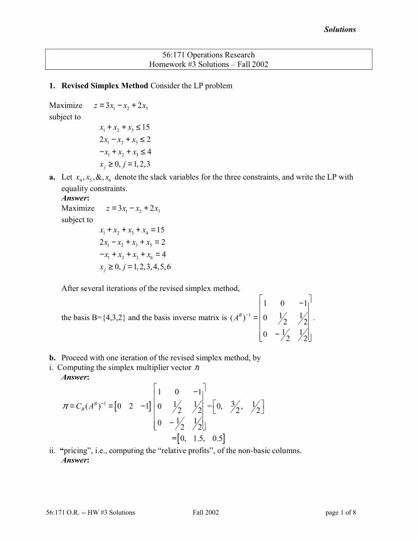
1. Revised Simplex Method Consider the LP problem

Maximize 1 2 33 2z x x x= − +subject to

1 2 3 15x x x+ + ≤

1 2 32 2x x x− + ≤

1 2 3 4x x x− + + ≤0, 1, 2,3jx j≥ =

a. Let 4 5 6, ,&,x x x denote the slack variables for the three constraints, and write the LP withequality constraints.Answer:Maximize 1 2 33 2z x x x= − +subject to

1 2 3 4 15x x x x+ + + =

1 2 3 52 2x x x x− + + =

1 2 3 6 4x x x x− + + + =0, 1, 2,3, 4,5,6jx j≥ =

After several iterations of the revised simplex method,

the basis B={4,3,2} and the basis inverse matrix is 1

1 0 11 1( ) 0 2 21 10 2 2

BA −

− = −

.

b. Proceed with one iteration of the revised simplex method, byi. Computing the simplex multiplier vector π

Answer:

[ ]1( ) 0 2 1BBC Aπ −= = −

1 0 11 10 2 21 10 2 2

− −

= 3 10, ,2 2

=[ ]0, 1.5, 0.5ii. “pricing”, i.e., computing the “relative profits”, of the non-basic columns.

Answer:

Solutions


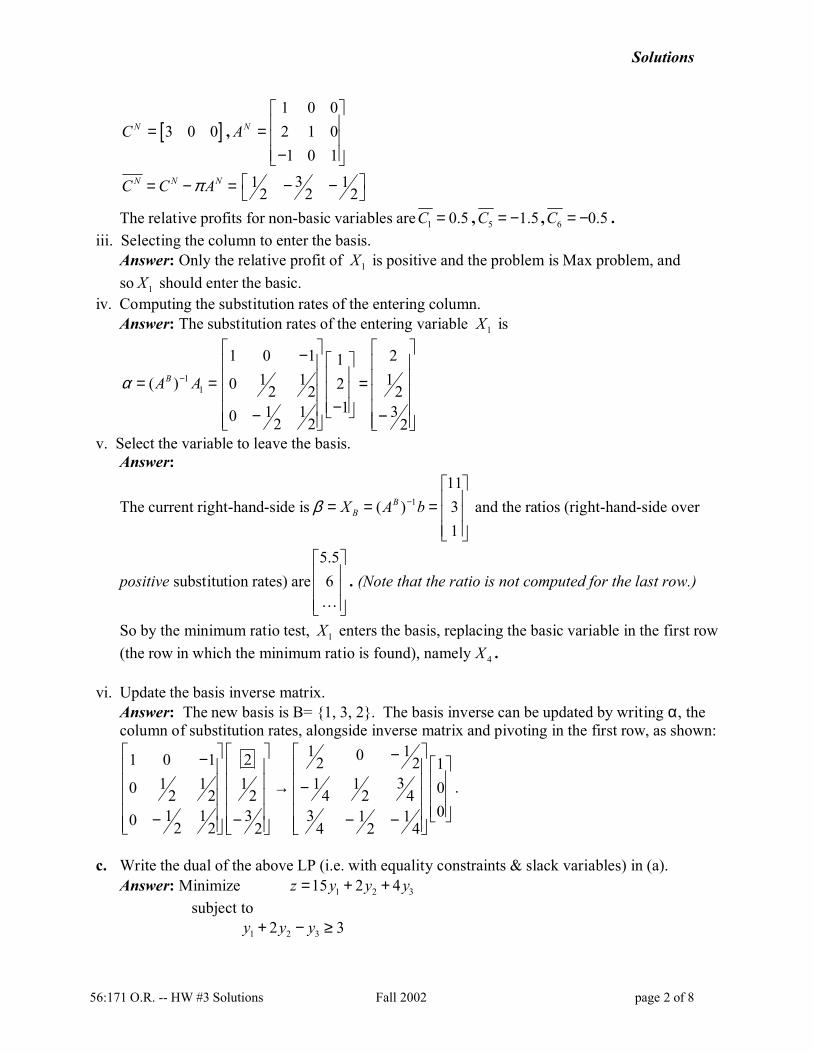
[ ]3 0 0NC = ,1 0 02 1 01 0 1

NA = −

N N NC C Aπ= − = 31 12 2 2

− − The relative profits for non-basic variables are 1 0.5C = , 5 1.5C = − , 6 0.5C = − .

iii. Selecting the column to enter the basis.Answer: Only the relative profit of 1X is positive and the problem is Max problem, andso 1X should enter the basic.

iv. Computing the substitution rates of the entering column.Answer: The substitution rates of the entering variable 1X is

11( )BA Aα −= =

1 0 1 211 1 10 22 2 2

11 1 30 2 2 2

− = − − −

v. Select the variable to leave the basis.Answer:

The current right-hand-side is 1

11( ) 3

1

BBX A bβ −

= = =

and the ratios (right-hand-side over

positive substitution rates) are5.56

. (Note that the ratio is not computed for the last row.)

So by the minimum ratio test, 1X enters the basis, replacing the basic variable in the first row(the row in which the minimum ratio is found), namely 4X .

vi. Update the basis inverse matrix.Answer: The new basis is B= {1, 3, 2}. The basis inverse can be updated by writing α, thecolumn of substitution rates, alongside inverse matrix and pivoting in the first row, as shown:

1 101 0 1 2 2 2 131 1 1 1 10 02 2 2 4 2 4

01 1 3 3 1 10 2 2 2 4 2 4

−− → − − − − −

.

c. Write the dual of the above LP (i.e. with equality constraints & slack variables) in (a).Answer: Minimize 1 2 315 2 4z y y y= + +

subject to1 2 32 3y y y+ − ≥

Solutions


1 2 3 1y y y− + ≥ −

1 2 3 2y y y+ + ≥0, 1, 2,3jy j≥ =

d. Substitute the vector π which you computed above in step (i) above to test whether it isfeasible in the dual LP. Which constraint(s) if any are violated? How does this relate to theresults in step (ii) above?Answer: If we substitute π = [ ]0, 1.5, 0.5 for the dual variables y, the first constraint

1 2 32 3y y y+ − ≥ is violated.Note: The simplex multipler vector π satisfies all the constraints in the dual problem if &only if the relative profits in (ii) are all non-positive (which implies that the solution isoptimal).

2. LP formulation: Staffing a Call Center (Case 3.3, pages 106-108, Intro. to O.R. by Hillier &Lieberman) Answer parts (a), (b), & (c) on page 108, using LINGO with sets to enter the model.

For the following analysis, consider the labor cost for the time employees spent answeringphones. The cost for paperwork time is charged to other cost centers.

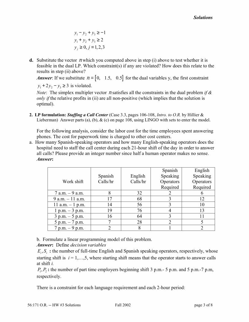
a. How many Spanish-speaking operators and how many English-speaking operators does thehospital need to staff the call center during each 21-hour shift of the day in order to answerall calls? Please provide an integer number since half a human operator makes no sense.Answer:

Work shiftSpanishCalls/hr

EnglishCalls/hr

SpanishSpeakingOperatorsRequired

EnglishSpeakingOperatorsRequired

7 a.m. – 9 a.m. 8 32 2 69 a.m. – 11 a.m. 17 68 3 1211 a.m. – 1 p.m. 14 56 3 101 p.m. – 3 p.m. 19 76 4 133 p.m. – 5 p.m. 16 64 3 115 p.m. – 7 p.m. 7 28 2 57 p.m. – 9 p.m. 2 8 1 2

b. Formulate a linear programming model of this problem.Answer: Define decision variables

,i iE S : the number of full-time English and Spanish speaking operators, respectively, whosestarting shift is i = 1,…,5, where starting shift means that the operator starts to answer callsat shift i.

1 2,P P : the number of part time employers beginning shift 3 p.m.- 5 p.m. and 5 p.m.-7 p.m,respectively.

There is a constraint for each language requirement and each 2-hour period:

Solutions


Minimize 1 1 2 2 3 3 4 4 5 5 1 240 40 40 40 40 40 44 44 44 44 44 48E S E S E S E S E S P P+ + + + + + + + + + +subject to

1 6E ≥ (English-speaking operator rqmts)

2 12E ≥

1 3 10E E+ ≥

2 4 13E E+ ≥

3 5 1 11E E P+ + ≥

4 1 2 5E P P+ + ≥

5 2 2E P+ ≥

1 2S ≥ (Spanish-speaking operator rqmts)

2 3S ≥

1 3 3S S+ ≥

2 4 4S S+ ≥

3 5 3S S+ ≥

4 2S ≥

5 1S ≥, , 0i i jE S P ≥ for all i=1,…,7 and j=1,2.

c. Obtain an optimal solution for the LP model formulated in part (b)Answer:

OBJECTIVE FUNCTION VALUE

1) 1640.000

VARIABLE VALUE REDUCED COSTE1 6.000000 0.000000S1 2.000000 0.000000E2 12.000000 0.000000S2 3.000000 0.000000E3 5.000000 0.000000S3 2.000000 0.000000E4 1.000000 0.000000S4 2.000000 0.000000E5 2.000000 0.000000S5 1.000000 0.000000P1 4.000000 0.000000P2 0.000000 40.000000

ROW SLACK OR SURPLUS DUAL PRICES2) 0.000000 -40.0000003) 0.000000 0.0000004) 1.000000 0.0000005) 0.000000 -40.0000006) 0.000000 -40.0000007) 0.000000 -4.0000008) 0.000000 -4.000000

Solutions


9) 0.000000 -40.00000010) 0.000000 -40.00000011) 1.000000 0.00000012) 1.000000 0.00000013) 0.000000 -40.00000014) 0.000000 -44.00000015) 0.000000 -4.000000

LINGO model: This is a bigger challenge than most other models we’ve looked at. We definethe sets LANGUAGE, PERIOD, & SHIFT, and then the derived sets which I’ve arbitrarilynames A, B, & D. The attribute W (of set B) specifies which 2-hour period each shift isanswering phones: W(i,j) = 1 if shift i is working in period j, and 0 otherwise. These binaryvalues are then used to compute the pay for each shift and to impose the requirements foroperators during each period. I have here defined the decision variables X(k,i) = # of operatorsspeaking language k working shift i. Thus X(1,1) & X(2,1) are identical to the variables E1 & S1,respectively, in the model shown above. Because none of the part-time operators speak Spanish, the variables X(2,6) = X(2,7) = 0 (where Spanish is the 2nd language and the part-time shifts are#6&7).

MODEL:

SETS:LANGUAGE/E S/;PERIOD/1..7/: RATE ;! Shifts 1-5 are full-time, and 6&7 are part-time;SHIFT/1..7/: PAY ;A(LANGUAGE,PERIOD): REQMT;B(SHIFT,PERIOD): W;D(LANGUAGE,SHIFT): X;

ENDSETS

DATA:! RATE is rate of pay for each 2-hour work period;RATE=20 20 20 20 20 24 24;! REQMT(i,j) is requirement for operators speaking language i

during 2-hour work period j;REQMT= 6 12 10 13 11 5 2

2 3 3 4 3 2 1;! W(j,k) indicates whether operator working shift j

is answering phones during 2-hr work period k;W= 1 0 1 0 0 0 0

0 1 0 1 0 0 00 0 1 0 1 0 00 0 0 1 0 1 00 0 0 0 1 0 10 0 0 0 1 1 00 0 0 0 0 1 1;

ENDDATA

Solutions


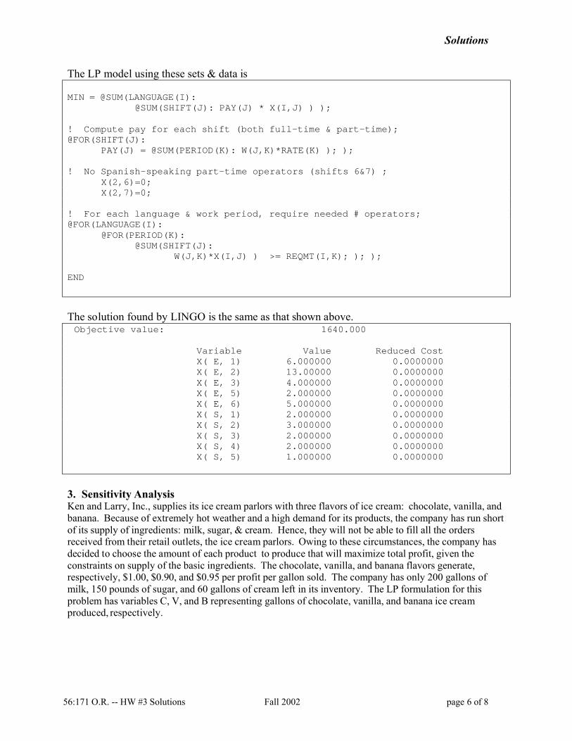
The LP model using these sets & data is

MIN = @SUM(LANGUAGE(I):@SUM(SHIFT(J): PAY(J) * X(I,J) ) );

! Compute pay for each shift (both full-time & part-time);@FOR(SHIFT(J):

PAY(J) = @SUM(PERIOD(K): W(J,K)*RATE(K) ); );

! No Spanish-speaking part-time operators (shifts 6&7) ;X(2,6)=0;X(2,7)=0;

! For each language & work period, require needed # operators;@FOR(LANGUAGE(I):

@FOR(PERIOD(K):@SUM(SHIFT(J):

W(J,K)*X(I,J) ) >= REQMT(I,K); ); );

END

The solution found by LINGO is the same as that shown above.Objective value: 1640.000

Variable Value Reduced CostX( E, 1) 6.000000 0.0000000X( E, 2) 13.00000 0.0000000X( E, 3) 4.000000 0.0000000X( E, 5) 2.000000 0.0000000X( E, 6) 5.000000 0.0000000X( S, 1) 2.000000 0.0000000X( S, 2) 3.000000 0.0000000X( S, 3) 2.000000 0.0000000X( S, 4) 2.000000 0.0000000X( S, 5) 1.000000 0.0000000

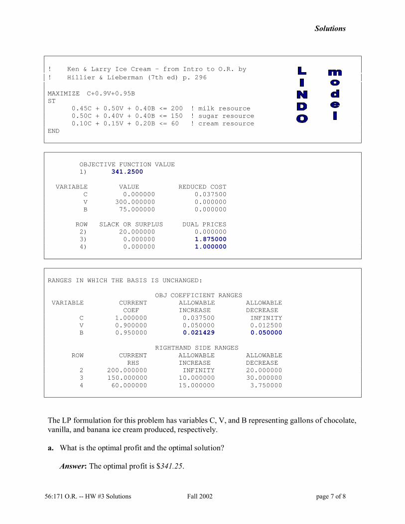
3. Sensitivity AnalysisKen and Larry, Inc., supplies its ice cream parlors with three flavors of ice cream: chocolate, vanilla, andbanana. Because of extremely hot weather and a high demand for its products, the company has run shortof its supply of ingredients: milk, sugar, & cream. Hence, they will not be able to fill all the ordersreceived from their retail outlets, the ice cream parlors. Owing to these circumstances, the company hasdecided to choose the amount of each product to produce that will maximize total profit, given theconstraints on supply of the basic ingredients. The chocolate, vanilla, and banana flavors generate,respectively, $1.00, $0.90, and $0.95 per profit per gallon sold. The company has only 200 gallons ofmilk, 150 pounds of sugar, and 60 gallons of cream left in its inventory. The LP formulation for thisproblem has variables C, V, and B representing gallons of chocolate, vanilla, and banana ice creamproduced, respectively.

Solutions


! Ken & Larry Ice Cream – from Intro to O.R. by! Hillier & Lieberman (7th ed) p. 296

MAXIMIZE C+0.9V+0.95BST

0.45C + 0.50V + 0.40B <= 200 ! milk resource0.50C + 0.40V + 0.40B <= 150 ! sugar resource0.10C + 0.15V + 0.20B <= 60 ! cream resource

END

OBJECTIVE FUNCTION VALUE1) 341.2500

VARIABLE VALUE REDUCED COSTC 0.000000 0.037500V 300.000000 0.000000B 75.000000 0.000000

ROW SLACK OR SURPLUS DUAL PRICES2) 20.000000 0.0000003) 0.000000 1.8750004) 0.000000 1.000000

RANGES IN WHICH THE BASIS IS UNCHANGED:

OBJ COEFFICIENT RANGESVARIABLE CURRENT ALLOWABLE ALLOWABLE

COEF INCREASE DECREASEC 1.000000 0.037500 INFINITYV 0.900000 0.050000 0.012500B 0.950000 0.021429 0.050000

RIGHTHAND SIDE RANGESROW CURRENT ALLOWABLE ALLOWABLE

RHS INCREASE DECREASE2 200.000000 INFINITY 20.0000003 150.000000 10.000000 30.0000004 60.000000 15.000000 3.750000

The LP formulation for this problem has variables C, V, and B representing gallons of chocolate,vanilla, and banana ice cream produced, respectively.

a. What is the optimal profit and the optimal solution?

Answer: The optimal profit is $341.25.

Solutions


The optimal quantities of the products are 0 gallons of chocolate ice cream, 300 gallons ofvanilla ice cream and 75 gallons of banana ice cream.

b. Suppose the profit per gallon of banana changes to $1.00. Will the optimal solution change,and what can be said about the effect on total profit?

Answer: An increase of profit of the banana ice cream to $1.00 is an increase of $0.05. Thisexceeds the “Allowable Increase” (0.021429) in which the basis is unchanged. So the basischanges, changing the optimal solution and the total profit (which would of course increase.)

c. Suppose the profit per gallon of banana changes to 92 cents. Will the optimal solutionchanges, and what can be said about the effect on total profit?

Answer: Because the decrease ($0.03) is less than the allowable decrease ($0.05) for whichthe basis is unchanged, the basic variables (& their values) are unchanged, but the total profitdecreases by $0.03/gal. × 75 gal. = $2.25.

d. Suppose the company discovers that 3 gallons of cream have gone sour and so must bethrown out. Will the optimal solution change, and what can be said about the effect on thetotal profit?Answer: The optimal solution would be changed because the quantity of cream whose slackis 0 is changed. Because the decrease (3 gal.) is less than the allowable decrease (which is3.75), the total profit would decrease by $3 (dual price of cream resource is $1.0/gal. so 3gal.× 1.0 $/gal. = $3).

e. Suppose that the company has the opportunity to buy an additional 15 pounds of sugar at atotal cost of $15. Should they buy it? Explain!

Answer: Inside the allowable range, the dual price is $1.875 so if 10 pounds of sugar isbought and used the profit increase by 10 × $1.875 = $18.75 which is more than the price of15 pounds of sugar and brings more profit (if 15 pounds of sugar is available, there would notbe less profit than when 10 pounds is used, and there possibly will be an additional increasein profit.) So the company should buy the 15 pounds of sugar at the stated price, since theywould obtain at least $18.75−$15.00 = $3.75 in additional net profits.

Solutions


56:171 Operations ResearchHomework #4 Solutions--Fall 2002

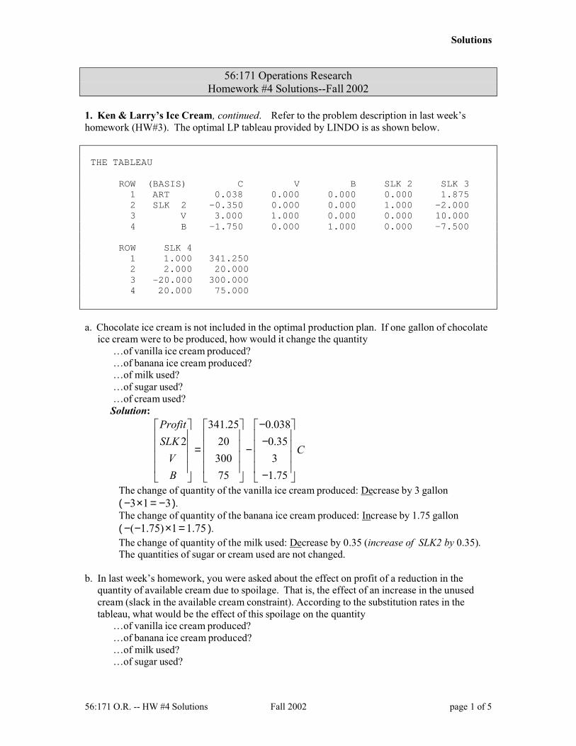
1. Ken & Larry’s Ice Cream, continued. Refer to the problem description in last week’shomework (HW#3). The optimal LP tableau provided by LINDO is as shown below.

THE TABLEAU

ROW (BASIS) C V B SLK 2 SLK 31 ART 0.038 0.000 0.000 0.000 1.8752 SLK 2 -0.350 0.000 0.000 1.000 -2.0003 V 3.000 1.000 0.000 0.000 10.0004 B -1.750 0.000 1.000 0.000 -7.500

ROW SLK 41 1.000 341.2502 2.000 20.0003 -20.000 300.0004 20.000 75.000

a. Chocolate ice cream is not included in the optimal production plan. If one gallon of chocolateice cream were to be produced, how would it change the quantity

…of vanilla ice cream produced?…of banana ice cream produced?…of milk used?…of sugar used?…of cream used?

Solution:341.25 0.038

2 20 0.35300 375 1.75

ProfitSLK

CVB

− − = − −

The change of quantity of the vanilla ice cream produced: Decrease by 3 gallon( 3 1 3− × = − ).The change of quantity of the banana ice cream produced: Increase by 1.75 gallon( ( 1.75) 1 1.75− − × = ).The change of quantity of the milk used: Decrease by 0.35 (increase of SLK2 by 0.35).The quantities of sugar or cream used are not changed.

b. In last week’s homework, you were asked about the effect on profit of a reduction in thequantity of available cream due to spoilage. That is, the effect of an increase in the unusedcream (slack in the available cream constraint). According to the substitution rates in thetableau, what would be the effect of this spoilage on the quantity

…of vanilla ice cream produced?…of banana ice cream produced?…of milk used?…of sugar used?

Solutions


Solution:341.25 1

2 20 24

300 2075 20

ProfitSLK

SLKVB

= − −

The spoilage implies that SLK4 is increased by 3 gallons.The change of quantity of the vanilla ice cream produced: Increase by 60 gallons(−(−20)×3 = 60). The change of quantity of the banana ice cream produced: Decrease by 60 gallons(−20×3 = −60).

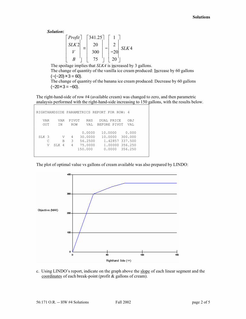
The right-hand-side of row #4 (available cream) was changed to zero, and then parametricanalaysis performed with the right-hand-side increasing to 150 gallons, with the results below.

RIGHTHANDSIDE PARAMETRICS REPORT FOR ROW: 4

VAR VAR PIVOT RHS DUAL PRICE OBJOUT IN ROW VAL BEFORE PIVOT VAL

0.0000 10.0000 0.000SLK 3 V 4 30.0000 10.0000 300.000

C B 3 56.2500 1.42857 337.500V SLK 4 4 75.0000 1.00000 356.250

150.000 0.0000 356.250

The plot of optimal value vs gallons of cream available was also prepared by LINDO:

c. Using LINDO’s report, indicate on the graph above the slope of each linear segment and thecoordinates of each break-point (profit & gallons of cream).

Solutions


❚❏❚❏❚❏❚❏❚❏❚❏❚❏❚❏❚❏❚❏❚❏❚❏❚❏❚❏❚❏❚❏❚❏❚❏❚❏❚❏❚❏❚❏❚❏❚❏❚❏❚❏❚❏❚❏❚❏❚❏❚

2. LP model formulation. Buster Sod’s younger brother, Marky Dee, operates three ranches inTexas. the acreage and irrigation water available for the three farms are shown below:

Farm AcreageWater available (acre-ft)

1 400 15002 600 20003 300 900

Three crops can be grown. However, the maximum acreage that can be grown of each crop islimited by the amount of appropriate harvesting equipment available. The three crops aredescribed below. Any combination of crops may be grown on a farm.

CropTotal harvesting capacity

(in acres)Water Reqmts (acre-ft per

acre)Expected profit

($/acre)Milo 700 6 400

Cotton 800 4 300Wheat 300 2 100

Using LINGO, the following sets were defined, with decision variables:

Xij = # acreas of crop j planted on farm i.

Solutions


MODEL: ! MARKY DEE SOD'S RANCHES;

SETS:FARM/1..3/:ACREAGE, H20_AVAIL;CROP/MILO, COTTON, WHEAT/:CAPACITY, H20_RQMT, PROFIT;COMBO(FARM,CROP):X;

ENDSETS

DATA:ACREAGE = 400 600 300;H20_AVAIL = 1500 2000 900;CAPACITY = 700 800 300;H20_RQMT = 6 4 2;PROFIT = 400 300 100;

ENDDATA

! INSERT OBJECTIVE & CONSTRAINTS HERE ;

END

a. Using LINGO, formulate the LP model to maximize the total expected profit of the threeranches. Solution:

MAX = @SUM(COMBO(I,J): PROFIT(J)*X(I,J) );@FOR(FARM(I):

@SUM(COMBO(I,J): X(I,J)) <= ACREAGE(I) ;@SUM(COMBO(I,J): H20_RQMT(J)*X(I,J)) <= H20_AVAIL(I) ;

);

@FOR(CROP(J):@SUM(COMBO(I,J): X(I,J)) <= CAPACITY(J) ;

);

b. Add the statements to the accompanying file (HW4_2.lg4) , and solve.Solution: The primal solution:

Variable Value Reduced CostX( 1, MILO) 0.0000000 0.0000000

X( 1, COTTON) 375.0000 0.0000000X( 1, WHEAT) 0.0000000 33.33333X( 2, MILO) 50.00000 0.0000000

X( 2, COTTON) 425.0000 0.0000000X( 2, WHEAT) 0.0000000 33.33333X( 3, MILO) 150.0000 0.0000000

X( 3, COTTON) 0.0000000 0.0000000X( 3, WHEAT) 0.0000000 33.33333

Solutions


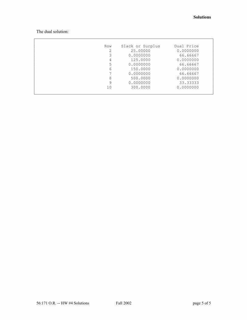
The dual solution:

Row Slack or Surplus Dual Price2 25.00000 0.00000003 0.0000000 66.666674 125.0000 0.00000005 0.0000000 66.666676 150.0000 0.00000007 0.0000000 66.666678 500.0000 0.00000009 0.0000000 33.3333310 300.0000 0.0000000

SOLUTION


56:171 Operations ResearchHomework #5 Solution– Fall 2002

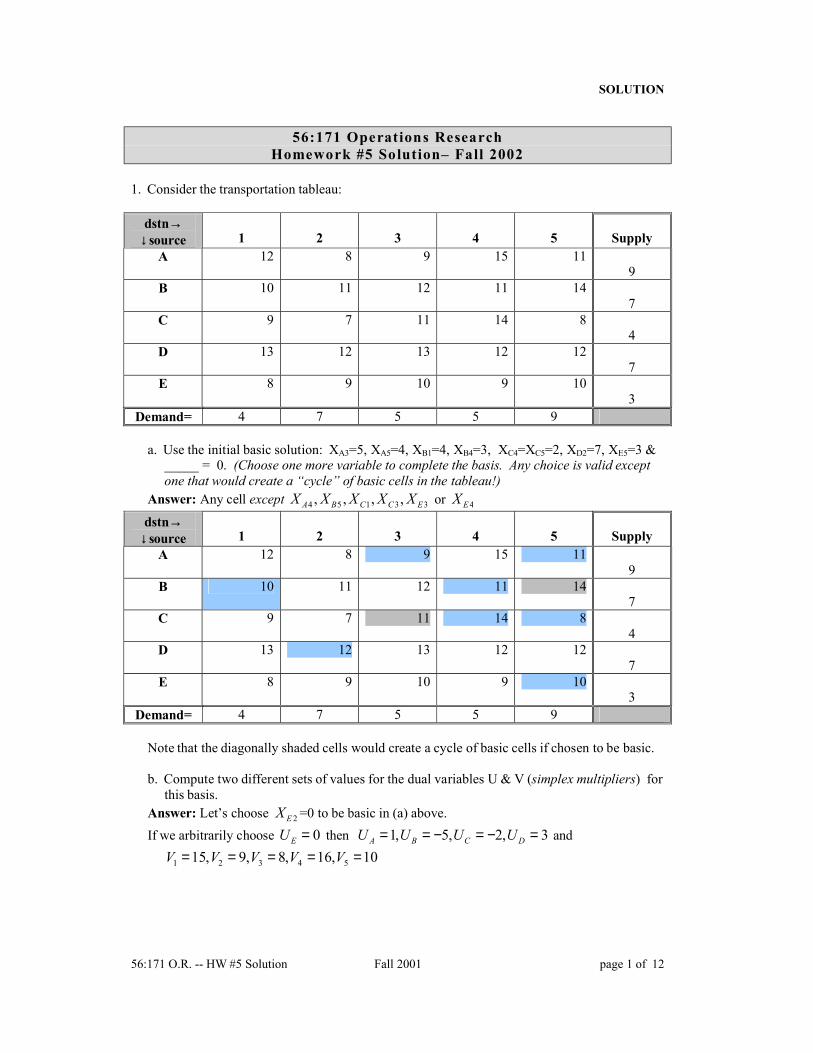
1. Consider the transportation tableau:

dstn→↓ source 1 2 3 4 5 Supply

A 12 8 9 15 119

B 10 11 12 11 147

C 9 7 11 14 84

D 13 12 13 12 127

E 8 9 10 9 103

Demand= 4 7 5 5 9

a. Use the initial basic solution: XA3=5, XA5=4, XB1=4, XB4=3, XC4=XC5=2, XD2=7, XE5=3 &_____ = 0. (Choose one more variable to complete the basis. Any choice is valid exceptone that would create a “cycle” of basic cells in the tableau!)

Answer: Any cell except 4 5 1 3 3, , , ,A B C C EX X X X X or 4EXdstn→

↓ source 1 2 3 4 5 SupplyA 12 8 9 15 11

9B 10 11 12 11 14

7C 9 7 11 14 8

4D 13 12 13 12 12

7E 8 9 10 9 10

3Demand= 4 7 5 5 9

Note that the diagonally shaded cells would create a cycle of basic cells if chosen to be basic.

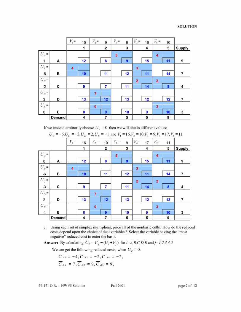
b. Compute two different sets of values for the dual variables U & V (simplex multipliers) forthis basis.

Answer: Let’s choose 2EX =0 to be basic in (a) above.If we arbitrarily choose 0EU = then 1, 5, 2, 3A B C DU U U U= = − = − = and

1 2 3 4 515, 9, 8, 16, 10V V V V V= = = = =

SOLUTION


1V = 15 2V = 9 3V = 8 4V = 16 5V = 101 2 3 4 5 Supply

AU = 5 41 A 12 8 9 15 11 9

BU = 4 3-5 B 10 11 12 11 14 7

CU = 2 2-2 C 9 7 11 14 8 4

DU = 73 D 13 12 13 12 12 7

EU = 0 30 E 8 9 10 9 10 3

Demand 4 7 5 5 9

If we instead arbitrarily choose 0AU = then we will obtain different values:6, 3, 2, 1B C D EU U U U= − = − = = − and 1 2 3 4 516, 10, 9, 17, 11V V V V V= = = = =

1V = 16 2V = 10 3V = 9 4V = 17 5V = 111 2 3 4 5 Supply

AU = 5 40 A 12 8 9 15 11 9

BU = 4 3-6 B 10 11 12 11 14 7

CU = 2 2-3 C 9 7 11 14 8 4

DU = 72 D 13 12 13 12 12 7

EU = 0 3-1 E 8 9 10 9 10 3

Demand 4 7 5 5 9

c. Using each set of simplex multipliers, price all of the nonbasic cells. How do the reducedcosts depend upon the choice of dual variables? Select the variable having the “mostnegative” reduced cost to enter the basis.

Answer: By calculating ( )ij ij i jC C U V= − + for i=A,B,C,D,E and j=1,2,3,4,5

We can get the following reduced costs, when 0EU = .

1 2 4

2 3 5

4 , 2 , 2 ,

7 , 9 , 9 ,A A A

B B B

C C C

C C C

= − = − = −

= = =

SOLUTION


1 2 3

1 3 4 5

1 3 4

4, 0, 5,

5, 2, 7, 1,

7, 2, 7

C C C

D D D D

E E E

C C C

C C C C

C C C

= − = =

= − = = − = −

= − == = −

When 0AU = , the results are exactly the same—the reduced costs depend on the sums (Ui

+ Vj), not on the values Ui & Vj individually!

The “most negative” (i.e., smallest) reduced cost is −7, which is that of each of the nonbasicvariables 4 1 4, ,D E EX X X .

d. What variable will leave the basis as the new variable enters the basis?

Answer: If, for example, we chose 4EX as a new basic variable then 4CX must leave thebasis.

e. Complete the computation of the optimal solution, using the transportation simplex method.

Answer: The optimal solution is the following.2 3

1 4

2 5

5

4 5

4, 5,4, 3,3, 1,7,2, 1

A A

B B

C C

D

E E

X XX XX XXX X

= == == === =

and all others are 0.

Cost = 291 (Solution is optimal!)

Next table is the following

1V = 9 2V = 10 3V = 9 4V = 10 5V = 111 2 3 4 5 Supply

AU = 3 -2 5 5 40 A 12 8 9 15 11 9

BU = 4 0 1 3 21 B 10 11 12 11 14 7

CU = 3 0 5 7 4-3 C 9 7 11 14 8 4

DU = 2 7 2 0 -12 D 13 12 13 12 12 7

EU = 0 0 2 2 1-1 E 8 9 10 9 10 3

Demand 4 7 5 5 9

SOLUTION


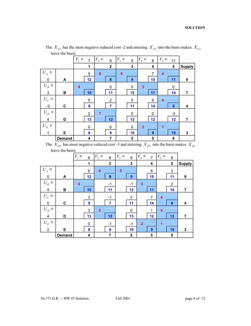
The 2AX has the most negative reduced cost -2 and entering 2AX into the basis makes 2EXleave the basis:

1V = 7 2V = 8 3V = 9 4V = 8 5V = 111 2 3 4 5 Supply

AU = 5 0 5 7 40 A 12 8 9 15 11 9

BU = 4 0 0 3 03 B 10 11 12 11 14 7

CU = 5 2 5 9 4-3 C 9 7 11 14 8 4

DU = 2 7 0 0 -34 D 13 12 13 12 12 7

EU = 0 0 0 2 11 E 8 9 10 9 10 3

Demand 4 7 5 5 9The 5DX has most negative reduced cost -3 and entering 5DX into the basis makes 5AX

leave the basis:

1V = 6 2V = 8 3V = 9 4V = 7 5V = 81 2 3 4 5 Supply

AU = 6 4 5 8 30 A 12 8 9 15 11 9

BU = 4 -1 -1 3 24 B 10 11 12 11 14 7

CU = 3 -1 2 7 40 C 9 7 11 14 8 4

DU = 3 3 0 1 44 D 13 12 13 12 12 7

EU = 0 -1 -1 2 12 E 8 9 10 9 10 3

Demand 4 7 5 5 9

SOLUTION


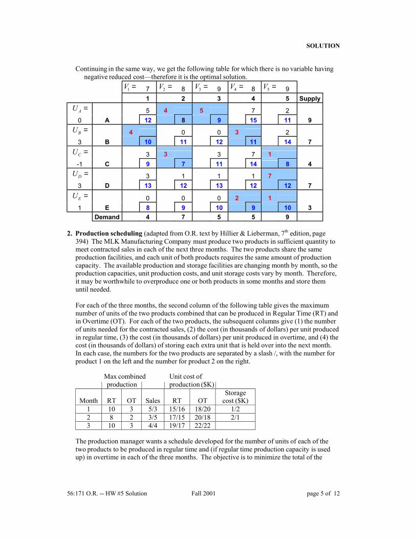
Continuing in the same way, we get the following table for which there is no variable havingnegative reduced cost—therefore it is the optimal solution.

1V = 7 2V = 8 3V = 9 4V = 8 5V = 91 2 3 4 5 Supply

AU = 5 4 5 7 20 A 12 8 9 15 11 9

BU = 4 0 0 3 23 B 10 11 12 11 14 7

CU = 3 3 3 7 1-1 C 9 7 11 14 8 4

DU = 3 1 1 1 73 D 13 12 13 12 12 7

EU = 0 0 0 2 11 E 8 9 10 9 10 3

Demand 4 7 5 5 9

2. Production scheduling (adapted from O.R. text by Hillier & Lieberman, 7th edition, page394) The MLK Manufacturing Company must produce two products in sufficient quantity tomeet contracted sales in each of the next three months. The two products share the sameproduction facilities, and each unit of both products requires the same amount of productioncapacity. The available production and storage facilities are changing month by month, so theproduction capacities, unit production costs, and unit storage costs vary by month. Therefore,it may be worthwhile to overproduce one or both products in some months and store themuntil needed.

For each of the three months, the second column of the following table gives the maximumnumber of units of the two products combined that can be produced in Regular Time (RT) andin Overtime (OT). For each of the two products, the subsequent columns give (1) the numberof units needed for the contracted sales, (2) the cost (in thousands of dollars) per unit producedin regular time, (3) the cost (in thousands of dollars) per unit produced in overtime, and (4) thecost (in thousands of dollars) of storing each extra unit that is held over into the next month. In each case, the numbers for the two products are separated by a slash /, with the number forproduct 1 on the left and the number for product 2 on the right.

Max combined Unit cost of| production | | production ($K)|

Month RT OT Sales RT OTStorage

cost ($K)1 10 3 5/3 15/16 18/20 1/22 8 2 3/5 17/15 20/18 2/13 10 3 4/4 19/17 22/22

The production manager wants a schedule developed for the number of units of each of thetwo products to be produced in regular time and (if regular time production capacity is usedup) in overtime in each of the three months. The objective is to minimize the total of the

SOLUTION


production and storage costs while meeting the contracted sales for each month. There is noinitial inventory, and no final inventory is desired after the three months.

a. Formulate this problem as a balanced transportation problem by constructing theappropriate transportation tableau.

b. Use the Northwest Corner Method to find an initial basic feasible solution. Is itdegenerate?

Answer for a) and b): The solution is not degenerate.

1A 1B 2A 2B 3A 3B EXCESS SUPPLY5 3 2

R1 15 16 16 18 18 19 0 101 2

O1 18 20 19 22 21 23 0 33 4 1

R2 inf inf 17 15 19 16 0 82

O2 inf inf 20 18 22 19 0 21 9

R3 inf inf inf inf 19 17 0 103

O3 inf inf inf inf 22 22 0 35 3 3 5 4 4 12SUM=410

c. Use the transportation simplex algorithm to find the optimal solution. Is it degenerate? Arethere multiple optima?

Answer: The optimal solution is the following.

1A 1B 2A 2B 3A 3B EXCESS SUPPLY5 3 2

R1 15 16 16 18 18 19 0 103

O1 18 20 19 22 21 23 0 31 5 2

R2 inf inf 17 15 19 16 0 82

O2 inf inf 20 18 22 19 0 24 2 4

R3 inf inf inf inf 19 17 0 103

O3 inf inf inf inf 22 22 0 3Demand 5 3 3 5 4 4 12SUM=389

SOLUTION


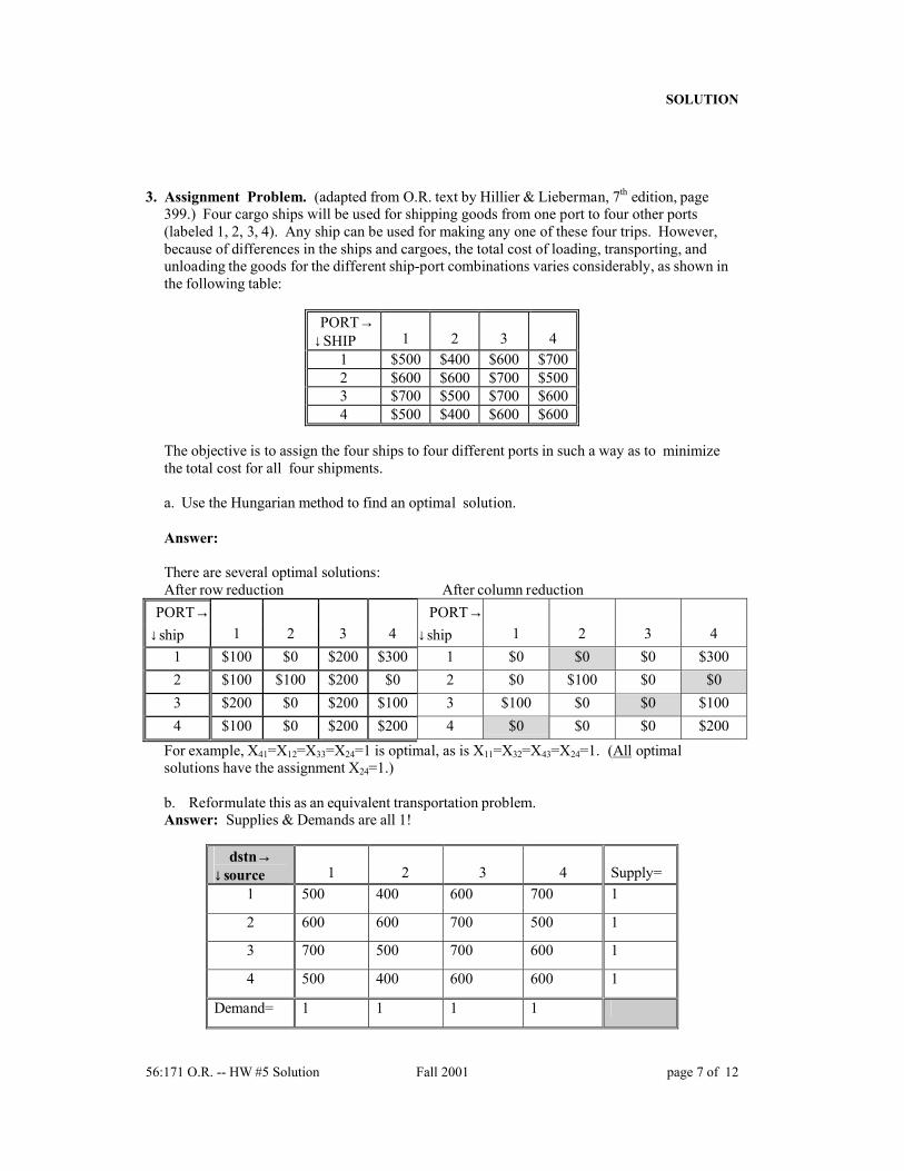
3. Assignment Problem. (adapted from O.R. text by Hillier & Lieberman, 7th edition, page399.) Four cargo ships will be used for shipping goods from one port to four other ports(labeled 1, 2, 3, 4). Any ship can be used for making any one of these four trips. However,because of differences in the ships and cargoes, the total cost of loading, transporting, andunloading the goods for the different ship-port combinations varies considerably, as shown inthe following table:

PORT→↓SHIP 1 2 3 4

1 $500 $400 $600 $7002 $600 $600 $700 $5003 $700 $500 $700 $6004 $500 $400 $600 $600

The objective is to assign the four ships to four different ports in such a way as to minimizethe total cost for all four shipments.

a. Use the Hungarian method to find an optimal solution.

Answer:

There are several optimal solutions:After row reduction After column reduction

PORT→ PORT→ ↓ship 1 2 3 4 ↓ship 1 2 3 4

1 $100 $0 $200 $300 1 $0 $0 $0 $3002 $100 $100 $200 $0 2 $0 $100 $0 $03 $200 $0 $200 $100 3 $100 $0 $0 $1004 $100 $0 $200 $200 4 $0 $0 $0 $200

For example, X41=X12=X33=X24=1 is optimal, as is X11=X32=X43=X24=1. (All optimalsolutions have the assignment X24=1.)

b. Reformulate this as an equivalent transportation problem.Answer: Supplies & Demands are all 1!

dstn→↓ source 1 2 3 4 Supply=

1 500 400 600 700 1

2 600 600 700 500 1

3 700 500 700 600 1

4 500 400 600 600 1

Demand= 1 1 1 1

SOLUTION


c. Use the Northwest Corner Method to obtain an initial basic feasible solution. (This will be adegenerate solution. Be sure to specify which variables are basic!)

Answer: Let the shaded cells form the initial basis.1 2 3 4 SUPPLY

11 500 400 600 700 1

12 600 600 700 500 1

13 700 500 700 600 1

14 500 400 600 600 1

Demand 1 1 1 1

d. Use the transportation simplex method to find the optimal solution.Answer:

500 400 500 4001 2 3 4 SUPPLY

1 0 100 3000 1 500 400 600 700 1

-100 1 0 -100200 2 600 600 700 500 1

0 -100 1 0200 3 700 500 700 600 1

-200 -200 -100 1200 4 500 400 600 600 1

Demand 1 1 1 1

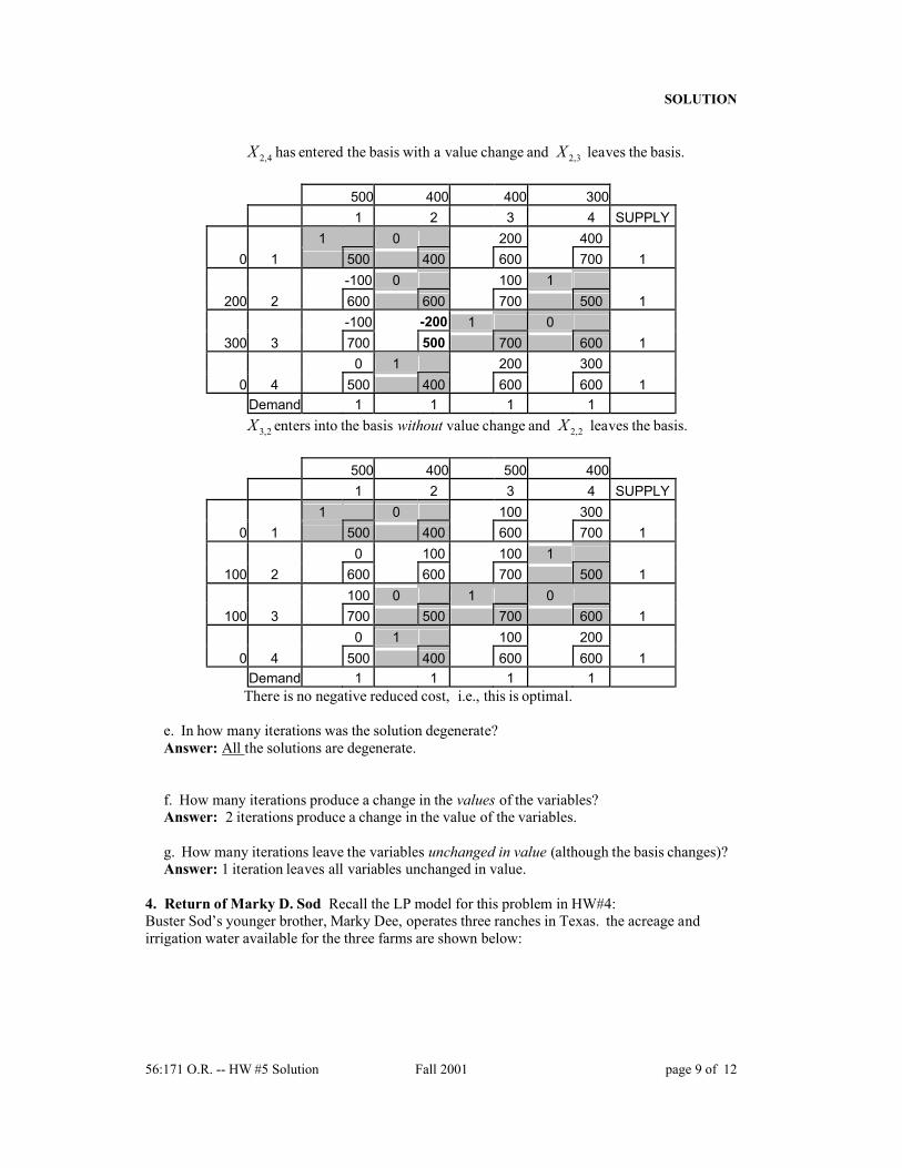
4,2X enters into the basis with value change and 4,4X leaves the basis.(Assignments, & therefore cost as well, have changed.)

500 400 500 4001 2 3 4 SUPPLY

1 0 100 3000 1 500 400 600 700 1

-100 0 1 -100200 2 600 600 700 500 1

0 -100 0 1200 3 700 500 700 600 1

0 1 100 2000 4 500 400 600 600 1Demand 1 1 1 1

SOLUTION


2,4X has entered the basis with a value change and 2,3X leaves the basis.

500 400 400 3001 2 3 4 SUPPLY

1 0 200 4000 1 500 400 600 700 1

-100 0 100 1200 2 600 600 700 500 1

-100 -200 1 0300 3 700 500 700 600 1

0 1 200 3000 4 500 400 600 600 1Demand 1 1 1 1

3,2X enters into the basis without value change and 2,2X leaves the basis.

500 400 500 4001 2 3 4 SUPPLY

1 0 100 3000 1 500 400 600 700 1

0 100 100 1100 2 600 600 700 500 1

100 0 1 0100 3 700 500 700 600 1

0 1 100 2000 4 500 400 600 600 1Demand 1 1 1 1

There is no negative reduced cost, i.e., this is optimal.

e. In how many iterations was the solution degenerate?Answer: All the solutions are degenerate.

f. How many iterations produce a change in the values of the variables?Answer: 2 iterations produce a change in the value of the variables.

g. How many iterations leave the variables unchanged in value (although the basis changes)?Answer: 1 iteration leaves all variables unchanged in value.

4. Return of Marky D. Sod Recall the LP model for this problem in HW#4:Buster Sod’s younger brother, Marky Dee, operates three ranches in Texas. the acreage andirrigation water available for the three farms are shown below:

SOLUTION


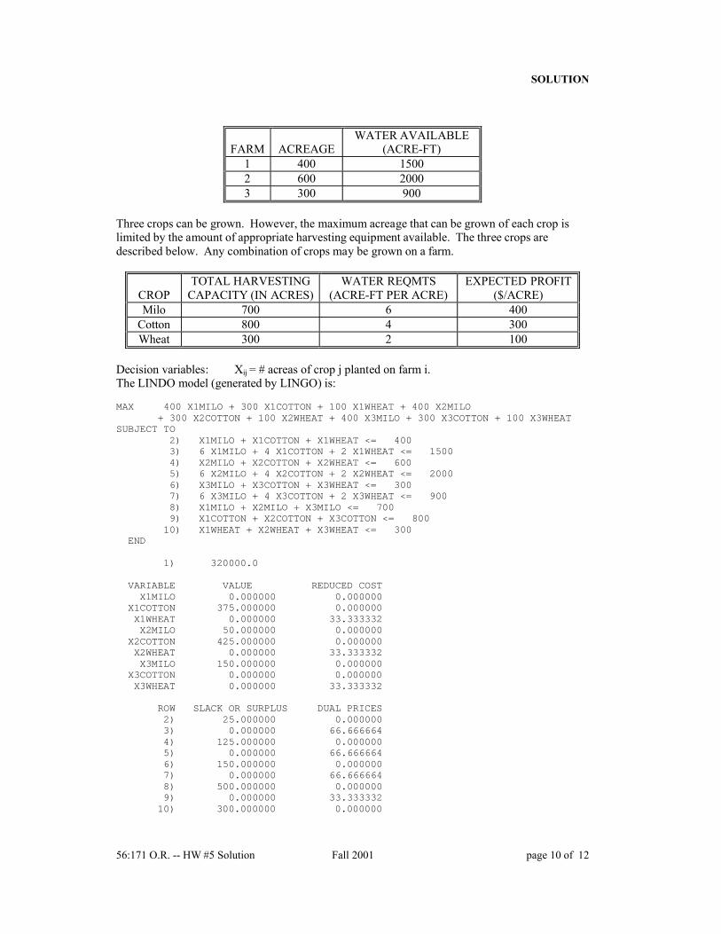
FARM ACREAGEWATER AVAILABLE

(ACRE-FT)1 400 15002 600 20003 300 900

Three crops can be grown. However, the maximum acreage that can be grown of each crop islimited by the amount of appropriate harvesting equipment available. The three crops aredescribed below. Any combination of crops may be grown on a farm.

CROPTOTAL HARVESTING

CAPACITY (IN ACRES)WATER REQMTS

(ACRE-FT PER ACRE)EXPECTED PROFIT

($/ACRE)Milo 700 6 400

Cotton 800 4 300Wheat 300 2 100

Decision variables: Xij = # acreas of crop j planted on farm i.The LINDO model (generated by LINGO) is:

MAX 400 X1MILO + 300 X1COTTON + 100 X1WHEAT + 400 X2MILO+ 300 X2COTTON + 100 X2WHEAT + 400 X3MILO + 300 X3COTTON + 100 X3WHEAT

SUBJECT TO2) X1MILO + X1COTTON + X1WHEAT <= 4003) 6 X1MILO + 4 X1COTTON + 2 X1WHEAT <= 15004) X2MILO + X2COTTON + X2WHEAT <= 6005) 6 X2MILO + 4 X2COTTON + 2 X2WHEAT <= 20006) X3MILO + X3COTTON + X3WHEAT <= 3007) 6 X3MILO + 4 X3COTTON + 2 X3WHEAT <= 9008) X1MILO + X2MILO + X3MILO <= 7009) X1COTTON + X2COTTON + X3COTTON <= 800

10) X1WHEAT + X2WHEAT + X3WHEAT <= 300END

1) 320000.0

VARIABLE VALUE REDUCED COSTX1MILO 0.000000 0.000000

X1COTTON 375.000000 0.000000X1WHEAT 0.000000 33.333332X2MILO 50.000000 0.000000

X2COTTON 425.000000 0.000000X2WHEAT 0.000000 33.333332X3MILO 150.000000 0.000000

X3COTTON 0.000000 0.000000X3WHEAT 0.000000 33.333332

ROW SLACK OR SURPLUS DUAL PRICES2) 25.000000 0.0000003) 0.000000 66.6666644) 125.000000 0.0000005) 0.000000 66.6666646) 150.000000 0.0000007) 0.000000 66.6666648) 500.000000 0.0000009) 0.000000 33.33333210) 300.000000 0.000000

SOLUTION


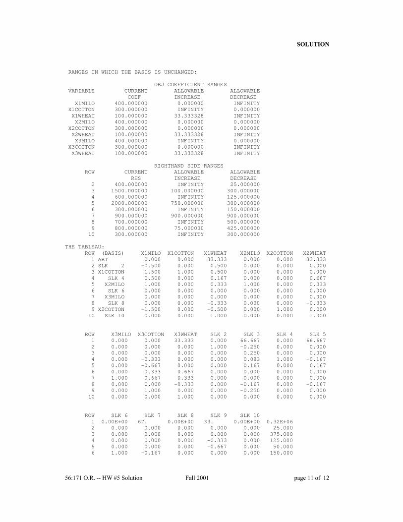
RANGES IN WHICH THE BASIS IS UNCHANGED:

OBJ COEFFICIENT RANGESVARIABLE CURRENT ALLOWABLE ALLOWABLE

COEF INCREASE DECREASEX1MILO 400.000000 0.000000 INFINITY

X1COTTON 300.000000 INFINITY 0.000000X1WHEAT 100.000000 33.333328 INFINITYX2MILO 400.000000 0.000000 0.000000

X2COTTON 300.000000 0.000000 0.000000X2WHEAT 100.000000 33.333328 INFINITYX3MILO 400.000000 INFINITY 0.000000

X3COTTON 300.000000 0.000000 INFINITYX3WHEAT 100.000000 33.333328 INFINITY

RIGHTHAND SIDE RANGESROW CURRENT ALLOWABLE ALLOWABLE

RHS INCREASE DECREASE2 400.000000 INFINITY 25.0000003 1500.000000 100.000000 300.0000004 600.000000 INFINITY 125.0000005 2000.000000 750.000000 300.0000006 300.000000 INFINITY 150.0000007 900.000000 900.000000 900.0000008 700.000000 INFINITY 500.0000009 800.000000 75.000000 425.00000010 300.000000 INFINITY 300.000000

THE TABLEAU:ROW (BASIS) X1MILO X1COTTON X1WHEAT X2MILO X2COTTON X2WHEAT1 ART 0.000 0.000 33.333 0.000 0.000 33.3332 SLK 2 -0.500 0.000 0.500 0.000 0.000 0.0003 X1COTTON 1.500 1.000 0.500 0.000 0.000 0.0004 SLK 4 0.500 0.000 0.167 0.000 0.000 0.6675 X2MILO 1.000 0.000 0.333 1.000 0.000 0.3336 SLK 6 0.000 0.000 0.000 0.000 0.000 0.0007 X3MILO 0.000 0.000 0.000 0.000 0.000 0.0008 SLK 8 0.000 0.000 -0.333 0.000 0.000 -0.3339 X2COTTON -1.500 0.000 -0.500 0.000 1.000 0.00010 SLK 10 0.000 0.000 1.000 0.000 0.000 1.000

ROW X3MILO X3COTTON X3WHEAT SLK 2 SLK 3 SLK 4 SLK 51 0.000 0.000 33.333 0.000 66.667 0.000 66.6672 0.000 0.000 0.000 1.000 -0.250 0.000 0.0003 0.000 0.000 0.000 0.000 0.250 0.000 0.0004 0.000 -0.333 0.000 0.000 0.083 1.000 -0.1675 0.000 -0.667 0.000 0.000 0.167 0.000 0.1676 0.000 0.333 0.667 0.000 0.000 0.000 0.0007 1.000 0.667 0.333 0.000 0.000 0.000 0.0008 0.000 0.000 -0.333 0.000 -0.167 0.000 -0.1679 0.000 1.000 0.000 0.000 -0.250 0.000 0.00010 0.000 0.000 1.000 0.000 0.000 0.000 0.000

ROW SLK 6 SLK 7 SLK 8 SLK 9 SLK 101 0.00E+00 67. 0.00E+00 33. 0.00E+00 0.32E+062 0.000 0.000 0.000 0.000 0.000 25.0003 0.000 0.000 0.000 0.000 0.000 375.0004 0.000 0.000 0.000 -0.333 0.000 125.0005 0.000 0.000 0.000 -0.667 0.000 50.0006 1.000 -0.167 0.000 0.000 0.000 150.000

SOLUTION


7 0.000 0.167 0.000 0.000 0.000 150.0008 0.000 -0.167 1.000 0.667 0.000 500.0009 0.000 0.000 0.000 1.000 0.000 425.00010 0.000 0.000 0.000 0.000 1.000 300.000

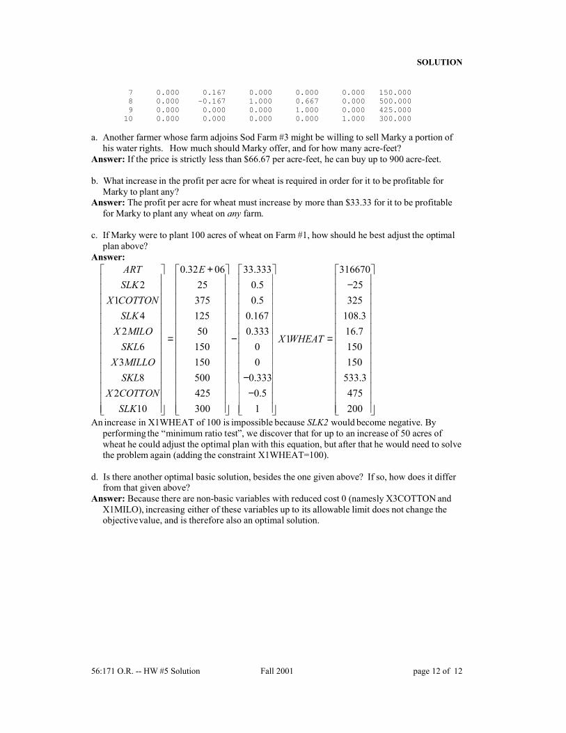
a. Another farmer whose farm adjoins Sod Farm #3 might be willing to sell Marky a portion ofhis water rights. How much should Marky offer, and for how many acre-feet?

Answer: If the price is strictly less than $66.67 per acre-feet, he can buy up to 900 acre-feet.

b. What increase in the profit per acre for wheat is required in order for it to be profitable forMarky to plant any?

Answer: The profit per acre for wheat must increase by more than $33.33 for it to be profitablefor Marky to plant any wheat on any farm.

c. If Marky were to plant 100 acres of wheat on Farm #1, how should he best adjust the optimalplan above?

Answer:0.32 06 33.333

2 25 0.51 375 0.5

4 125 0.1672 50 0.333

6 150 03 150 0

8 500 0.3332 425 0.5

10 300 1

ART ESLK

X COTTONSLK

X MILOSKL

X MILLOSKL

X COTTONSLK

+

= −

− −

31667025

325108.316.7

1150150

533.3475200

X WHEAT

−

=

An increase in X1WHEAT of 100 is impossible because SLK2 would become negative. Byperforming the “minimum ratio test”, we discover that for up to an increase of 50 acres ofwheat he could adjust the optimal plan with this equation, but after that he would need to solvethe problem again (adding the constraint X1WHEAT=100).

d. Is there another optimal basic solution, besides the one given above? If so, how does it differfrom that given above?

Answer: Because there are non-basic variables with reduced cost 0 (namesly X3COTTON andX1MILO), increasing either of these variables up to its allowable limit does not change theobjective value, and is therefore also an optimal solution.

SOLUTIONS

56:171 O.R. HW#7 Solutions Fall 2002 page 1 of 8

56:171 Operations ResearchHomework #7 Solutions -- Fall 2002

1. Decision Analysis (adapted from Exercise 15.2-7, page 784, Operations Research, 7th edition, byHillier & Lieberman.)Dwight Moody is the manager of a large farm with 1,000 acres of arable land. For greater efficiency,Dwight always devotes the farm to growing one crop at a time. He now needs to make a decision onwhich one of four crops to grow during the upcoming growing season. For each of these crops,Dwight has obtained the following estimates of crop yields and net incomes per bushel under variousweather conditions.

Weather Crop 1 Crop 2 Crop 3 Crop 4Dry 20 15 30 40Moderate 35 20 25 40Damp 40 30 25 40Net income/bushel $1.00 $1.50 $1.00 $0.50

After referring to historical meteorological records, Dwight also estimated the following probabilitiesfor the weather during the growing season:

Dry 0.3Moderate 0.5Damp 0.2

Using the criterion of “Maximize expected payoff”, determine which crop to grow.Solution: Expected payoffs

• Crop 1: (20 0.3 35 0.5 40 0.2) $1.00× + × + × × =$31.50• Crop 2: (15 0.3 20 0.5 30 0.2) $1.50 $30.75× + × + × × =• Crop 3: (30 0.3 25 0.5 25 0.2) $1.10 $26.50× + × + × × =• Crop 4: (40 0.3 40 0.5 40 0.2) $0.50 $20.00× + × + × × =Dwight Moody should choose crop 1 with $31.50 payoff.

2. Bayes’ Rule (Exercise 15.3-15, pp. 788-789, Operations Research, 7th edition, by Hillier &Lieberman)

There are two biased coins, coin A with probability of landing heads equal to 0.8 and the coin B withprobability of heads equal to 0.4. One coin is chosen at random (each with probability 50%) to betossed twice. You are to receive $100 if you correctly predict how many heads will occur in twotosses of this coin.

a. Using the “Maximum Expected Payoff” criterion, what is the optimal prediction, and what is thecorresponding expected payoff?

Solution: We are given P(H|A) = 0.8 and P(H|B) = 0.4P(2H | A) = (0.8)2 = 0.64 P(2H | B) = (0.4)2 = 0.16P(1H | A) = 1−0.64−0.04 = 0.32 P(2H | B) = 1−0.16−0.36 = 0.48P(0H | A) = (0.2)2 = 0.04 P(2H | B) = (0.6)2 = 0.36

P(2H) = P(2H | A)× P(A) + P(2H | B)× P(B) = 0.5×0.64 + 0.5×0.16 = 0.4P(1H) = P(1H | A)× P(A) + P(1H | B)× P(B) = 0.5×0.32 + 0.5×0.48 = 0.4P(0H) = P(0H | A)× P(A) + P(0H | B)× P(B) = 0.5×0.04 + 0.5×0.36 = 0.2

Should predict either 1 or 2 heads, each with expected payoff $40.00

SOLUTIONS


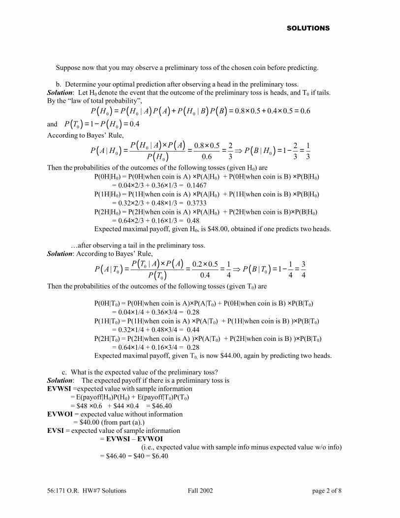
Suppose now that you may observe a preliminary toss of the chosen coin before predicting.

b. Determine your optimal prediction after observing a head in the preliminary toss. Solution: Let H0 denote the event that the outcome of the preliminary toss is heads, and T0 if tails.By the “law of total probability”,

( ) ( ) ( ) ( ) ( )0 0 0| | 0.8 0.5 0.4 0.5 0.6P H P H A P A P H B P B= + = × + × =

and ( ) ( )0 01 0.4P T P H= − =According to Bayes’ Rule,

( ) ( ) ( )( ) ( )0

0 00

| 0.8 0.5 2 2 1| | 10.6 3 3 3

P H A P AP A H P B H

P H× ×= = = ⇒ = − =

Then the probabilities of the outcomes of the following tosses (given H0) areP(0H|H0) = P(0H|when coin is A) ×P(A|H0) + P(0H|when coin is B) ×P(B|H0)

= 0.04×2/3 + 0.36×1/3 = 0.1467P(1H|H0) = P(1H|when coin is A) ×P(A|H0) + P(1H|when coin is B) ×P(B|H0)

= 0.32×2/3 + 0.48×1/3 = 0.3733P(2H|H0) = P(2H|when coin is A) ×P(A|H0) + P(2H|when coin is B)×P(B|H0)

= 0.64×2/3 + 0.16×1/3 = 0.48Expected maximal payoff, given H0, is $48.00, obtained if one predicts two heads.

…after observing a tail in the preliminary toss.Solution: According to Bayes’ Rule,

( ) ( ) ( )( ) ( )0

0 00

| 0.2 0.5 1 1 3| | 10.4 4 4 4

P T A P AP A T P B T

P T× ×= = = ⇒ = − =

Then the probabilities of the outcomes of the following tosses (given T0) are

P(0H|T0) = P(0H|when coin is A)×P(A|T0) + P(0H|when coin is B) ×P(B|T0)= 0.04×1/4 + 0.36×3/4 = 0.28

P(1H|T0) = P(1H|when coin is A) ×P(A|T0) + P(1H|when coin is B) )×P(B|T0)= 0.32×1/4 + 0.48×3/4 = 0.44

P(2H|T0) = P(2H|when coin is A) )×P(A|T0) + P(2H|when coin is B) )×P(B|T0)= 0.64×1/4 + 0.16×3/4 = 0.28

Expected maximal payoff, given T0, is now $44.00, again by predicting two heads.

c. What is the expected value of the preliminary toss?Solution: The expected payoff if there is a preliminary toss isEVWSI =expected value with sample information

= E(payoff|H0)P(H0) + E(payoff|T0)P(T0)= $48 ×0.6 + $44 ×0.4 = $46.40

EVWOI = expected value without information= $40.00 (from part (a).)

EVSI = expected value of sample information= EVWSI – EVWOI

(i.e., expected value with sample info minus expected value w/o info)= $46.40 − $40 = $6.40

SOLUTIONS


3. Integer Programming Model (based upon Case 12.3, page 649-653 of Operations Research, 7th

edition, by Hillier & Lieberman. See the text for the complete case description. What follows is acondensed version.)

Brenda Sims, the saleswoman on the floor at Furniture City, understood that Furniture City required anew inventory policy. Not only was the megastore losing money by making customers unhappy withdelivery delays, but it was also losing money by wasting warehouse space. By changing the inventorypolicy to stock only popular items and replenish them immediately when they are sold, Furniture Citywould ensure that the majority of customers receive their furniture immediately and that the valuablewarehouse space was utilized effectively.

She decided… to use her kitchen department as a model for the new inventory policy. She wouldidentify all kitchen sets comprising 85% of customers orders. Given the fixed amount of warehousespace allocated to the kitchen department, she would identify the items Furniture City should stock inorder to satisfy the greatest number of customer orders.

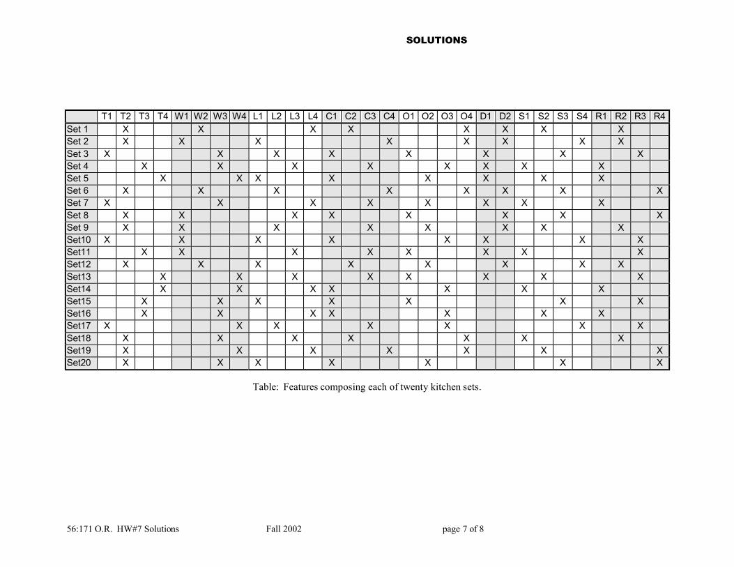
Brenda analyzed her records over the past three years and determined that 20 kitchen sets wereresponsible for 85% of customer orders. These 20 kitchen sets were composed of up to eight features,usually with four styles of each feature (except for the dishwashers, with two styles.)

• Floor tile: styles T1, T2, T3, T4• Wallpaper: styles W1, W2, W3, W4• Light fixtures: styles L1, L2, L3, L4• Cabinets: styles C1, C2, C3, C4• Countertops: styles O1, O2, O3, O4• Dishwashers: styles D1, D2• Sinks: styles S1, S2, S3, S4• Ranges: styles R1, R2, R3, R4

(Sets, 14 through 20, however, do not include dishwashers.)

The warehouse could hold 50 ft2 of tile and 12 rolls of wallpaper in the inventory bins. the inventoryshelves could hold two light fixtures, two cabinets, three countertops, and two sinks. Dishwashers andranges are similar in size, so Furniture City stored them in similar locations. The warehouse floorcould hold a total of four dishwashers and ranges.

Every kitchen set includes exactly 20 ft2 of tile and exactly 5 rolls of wallpaper. Therefore, 20 ft2 of aparticular style of tile and five rolls of a particular style of wallpaper are required for the styles to be instock.

SOLUTIONS


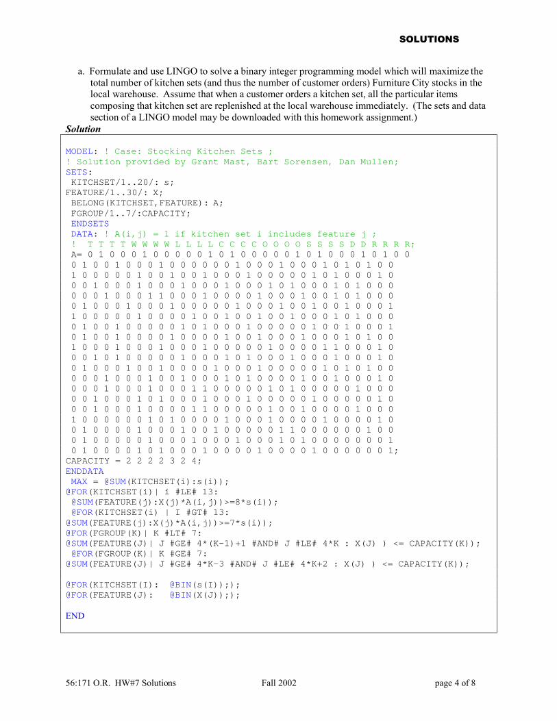
a. Formulate and use LINGO to solve a binary integer programming model which will maximize thetotal number of kitchen sets (and thus the number of customer orders) Furniture City stocks in thelocal warehouse. Assume that when a customer orders a kitchen set, all the particular itemscomposing that kitchen set are replenished at the local warehouse immediately. (The sets and datasection of a LINGO model may be downloaded with this homework assignment.)

Solution

MODEL: ! Case: Stocking Kitchen Sets ;! Solution provided by Grant Mast, Bart Sorensen, Dan Mullen;SETS:KITCHSET/1..20/: s;FEATURE/1..30/: X;BELONG(KITCHSET,FEATURE): A;FGROUP/1..7/:CAPACITY;ENDSETSDATA: ! A(i,j) = 1 if kitchen set i includes feature j ;! T T T T W W W W L L L L C C C C O O O O S S S S D D R R R R;A= 0 1 0 0 0 1 0 0 0 0 0 1 0 1 0 0 0 0 0 1 0 1 0 0 0 1 0 1 0 00 1 0 0 1 0 0 0 1 0 0 0 0 0 0 1 0 0 0 1 0 0 0 1 0 1 0 1 0 01 0 0 0 0 0 1 0 0 1 0 0 1 0 0 0 1 0 0 0 0 0 1 0 1 0 0 0 1 00 0 1 0 0 0 1 0 0 0 1 0 0 0 1 0 0 0 1 0 1 0 0 0 1 0 1 0 0 00 0 0 1 0 0 0 1 1 0 0 0 1 0 0 0 0 1 0 0 0 1 0 0 1 0 1 0 0 00 1 0 0 0 1 0 0 0 1 0 0 0 0 0 1 0 0 0 1 0 0 1 0 0 1 0 0 0 11 0 0 0 0 0 1 0 0 0 0 1 0 0 1 0 0 1 0 0 1 0 0 0 1 0 1 0 0 00 1 0 0 1 0 0 0 0 0 1 0 1 0 0 0 1 0 0 0 0 0 1 0 0 1 0 0 0 10 1 0 0 1 0 0 0 0 1 0 0 0 0 1 0 0 1 0 0 0 1 0 0 0 1 0 1 0 01 0 0 0 1 0 0 0 1 0 0 0 1 0 0 0 0 0 1 0 0 0 0 1 1 0 0 0 1 00 0 1 0 1 0 0 0 0 0 1 0 0 0 1 0 1 0 0 0 1 0 0 0 1 0 0 0 1 00 1 0 0 0 1 0 0 1 0 0 0 0 1 0 0 0 1 0 0 0 0 0 1 0 1 0 1 0 00 0 0 1 0 0 0 1 0 0 1 0 0 0 1 0 1 0 0 0 0 1 0 0 1 0 0 0 1 00 0 0 1 0 0 0 1 0 0 0 1 1 0 0 0 0 0 1 0 1 0 0 0 0 0 1 0 0 00 0 1 0 0 0 1 0 1 0 0 0 1 0 0 0 1 0 0 0 0 0 1 0 0 0 0 0 1 00 0 1 0 0 0 1 0 0 0 0 1 1 0 0 0 0 0 1 0 0 1 0 0 0 0 1 0 0 01 0 0 0 0 0 0 1 0 1 0 0 0 0 1 0 0 0 1 0 0 0 0 1 0 0 0 0 1 00 1 0 0 0 0 1 0 0 0 1 0 0 1 0 0 0 0 0 1 1 0 0 0 0 0 0 1 0 00 1 0 0 0 0 0 1 0 0 0 1 0 0 0 1 0 0 0 1 0 1 0 0 0 0 0 0 0 10 1 0 0 0 0 1 0 1 0 0 0 1 0 0 0 0 1 0 0 0 0 1 0 0 0 0 0 0 1;CAPACITY = 2 2 2 2 3 2 4;ENDDATAMAX = @SUM(KITCHSET(i):s(i));@FOR(KITCHSET(i)| i #LE# 13:@SUM(FEATURE(j):X(j)*A(i,j))>=8*s(i));@FOR(KITCHSET(i) | I #GT# 13:@SUM(FEATURE(j):X(j)*A(i,j))>=7*s(i));@FOR(FGROUP(K)| K #LT# 7:@SUM(FEATURE(J)| J #GE# 4*(K-1)+1 #AND# J #LE# 4*K : X(J) ) <= CAPACITY(K));@FOR(FGROUP(K)| K #GE# 7:@SUM(FEATURE(J)| J #GE# 4*K-3 #AND# J #LE# 4*K+2 : X(J) ) <= CAPACITY(K));

@FOR(KITCHSET(I): @BIN(s(I)););@FOR(FEATURE(J): @BIN(X(J)););

END

SOLUTIONS


The number of binary integer variables(20+30=50) exceeds the maximum number which is allowed bythe student version of LINGO. The solution shown below was found by using LINGO to create a file in“MPS” format which can be read by most solvers—in this case CPLEX.

SOLUTIONS


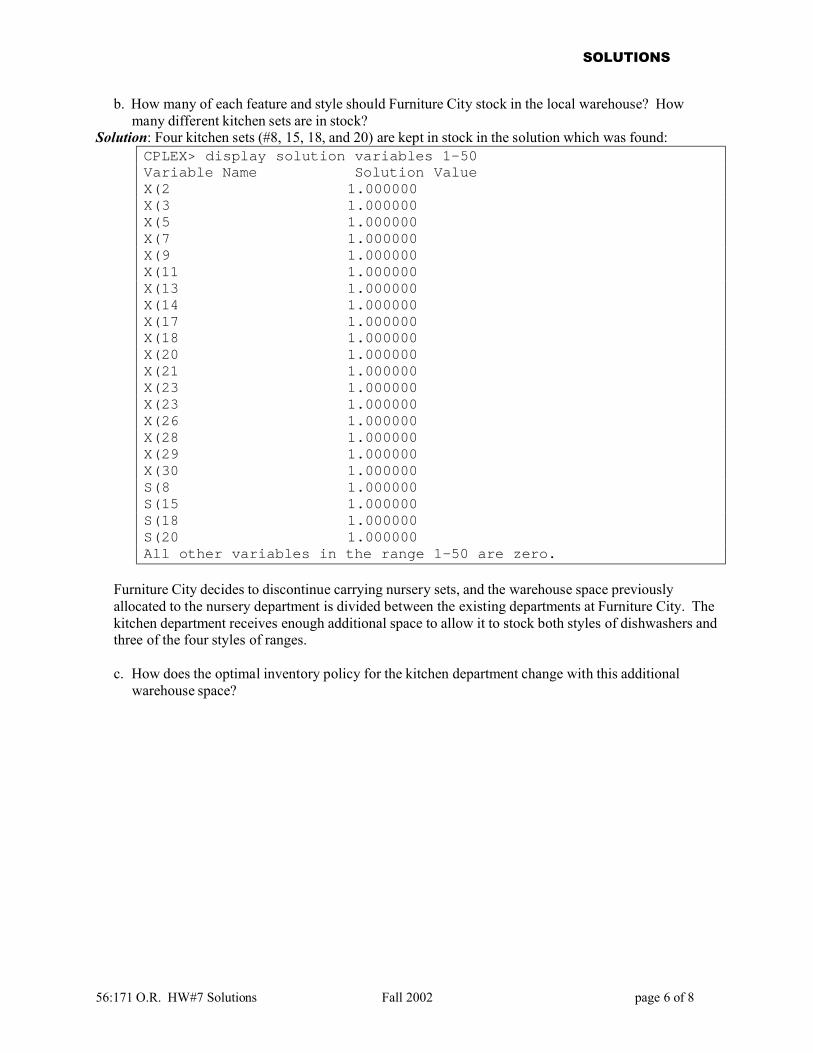
b. How many of each feature and style should Furniture City stock in the local warehouse? Howmany different kitchen sets are in stock?

Solution: Four kitchen sets (#8, 15, 18, and 20) are kept in stock in the solution which was found:CPLEX> display solution variables 1-50Variable Name Solution ValueX(2 1.000000X(3 1.000000X(5 1.000000X(7 1.000000X(9 1.000000X(11 1.000000X(13 1.000000X(14 1.000000X(17 1.000000X(18 1.000000X(20 1.000000X(21 1.000000X(23 1.000000X(23 1.000000X(26 1.000000X(28 1.000000X(29 1.000000X(30 1.000000S(8 1.000000S(15 1.000000S(18 1.000000S(20 1.000000All other variables in the range 1-50 are zero.

Furniture City decides to discontinue carrying nursery sets, and the warehouse space previouslyallocated to the nursery department is divided between the existing departments at Furniture City. Thekitchen department receives enough additional space to allow it to stock both styles of dishwashers andthree of the four styles of ranges.

c. How does the optimal inventory policy for the kitchen department change with this additionalwarehouse space?

SOLUTIONS


T1 T2 T3 T4 W1 W2 W3 W4 L1 L2 L3 L4 C1 C2 C3 C4 O1 O2 O3 O4 D1 D2 S1 S2 S3 S4 R1 R2 R3 R4Set 1 X X X X X X X XSet 2 X X X X X X X XSet 3 X X X X X X X XSet 4 X X X X X X X XSet 5 X X X X X X X XSet 6 X X X X X X X XSet 7 X X X X X X X XSet 8 X X X X X X X XSet 9 X X X X X X X XSet10 X X X X X X X XSet11 X X X X X X X XSet12 X X X X X X X XSet13 X X X X X X X XSet14 X X X X X X XSet15 X X X X X X XSet16 X X X X X X XSet17 X X X X X X XSet18 X X X X X X XSet19 X X X X X X XSet20 X X X X X X X

Table: Features composing each of twenty kitchen sets.

SOLUTIONS


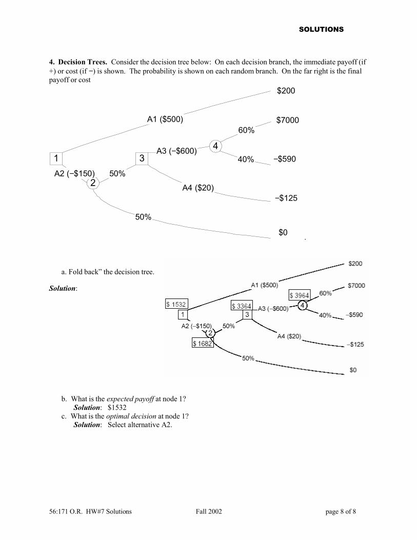
4. Decision Trees. Consider the decision tree below: On each decision branch, the immediate payoff (if+) or cost (if −) is shown. The probability is shown on each random branch. On the far right is the finalpayoff or cost

3

2

4

A1 ($500)

A2 (−$150) 50%

A3 (−$600)

A4 ($20)

50%

60%

40%

$0

−$125

−$590

$7000

$200

1

.

a. Fold back” the decision tree.

Solution:

b. What is the expected payoff at node 1?Solution: $1532

c. What is the optimal decision at node 1?Solution: Select alternative A2.

SOLUTION

56:171 O.R. HW#8 Solution Fall 2002 page 1 of 5

56:171 Operations ResearchHomework #8 Solution -- Fall 2002

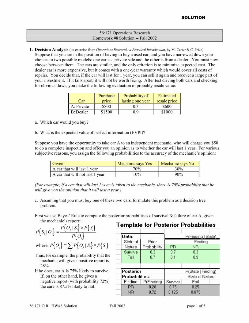
1. Decision Analysis (an exercise from Operations Research: a Practical Introduction, by M. Carter & C. Price)Suppose that you are in the position of having to buy a used car, and you have narrowed down yourchoices to two possible models: one car is a private sale and the other is from a dealer. You must nowchoose between them. The cars are similar, and the only criterion is to minimize expected cost. Thedealer car is more expensive, but it comes with a one-year warranty which would cover all costs ofrepairs. You decide that, if the car will last for 1 year, you can sell it again and recover a large part ofyour investment. If it falls apart, it will not be worth fixing. After test driving both cars and checkingfor obvious flaws, you make the following evaluation of probably resale value:

CarPurchase

priceProbability of

lasting one yearEstimated

resale priceA: Private $800 0.3 $600B: Dealer $1500 0.9 $1000

a. Which car would you buy?

b. What is the expected value of perfect information (EVPI)?

Suppose you have the opportunity to take car A to an independent mechanic, who will charge you $50to do a complete inspection and offer you an opinion as to whether the car will last 1 year. For varioussubjective reasons, you assign the following probabiliities to the accuracy of the mechanic’s opinion:

Given: Mechanic says Yes Mechanic says NoA car that will last 1 year 70% 30%A car that will not last 1 year 10% 90%

(For example, if a car that will last 1 year is taken to the mechanic, there is 70% probability that hewill give you the opinion that it will last a year.)

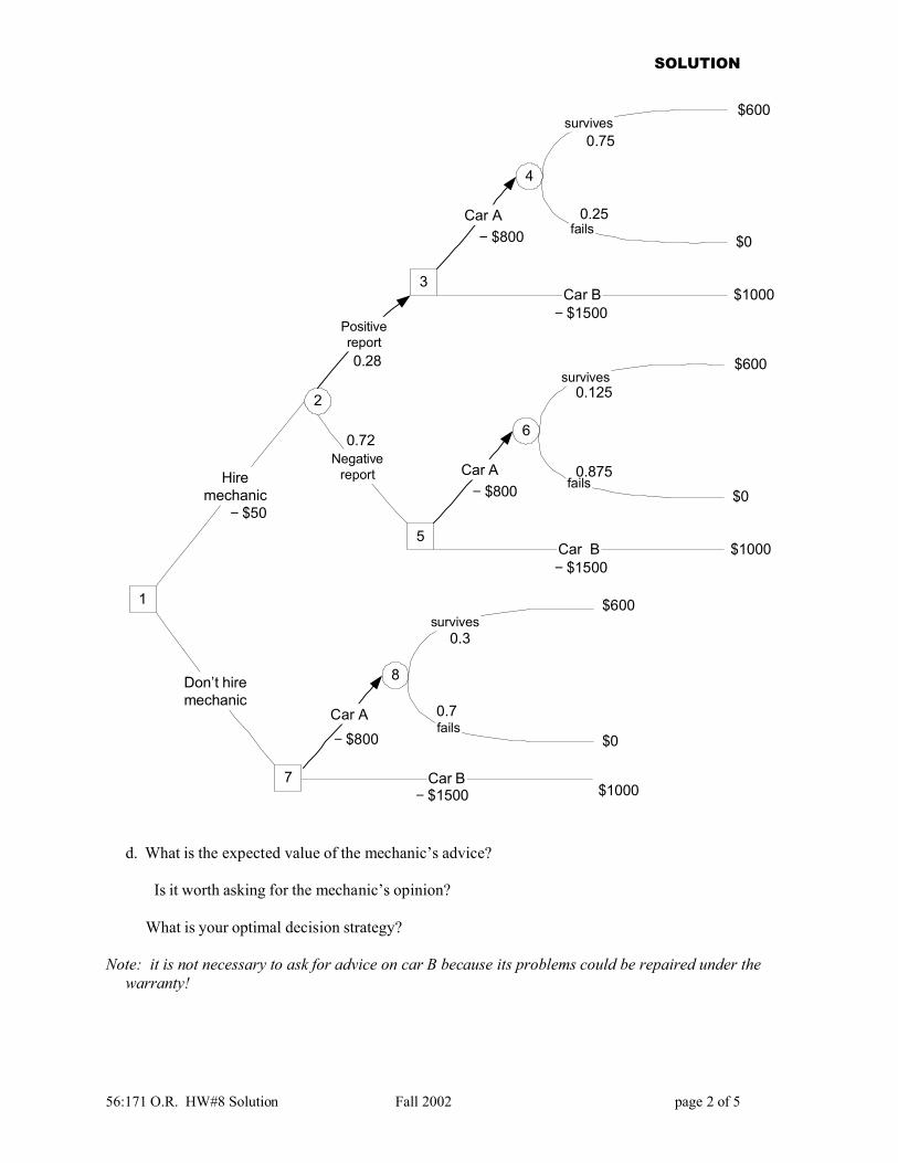
c. Assuming that you must buy one of these two cars, formulate this problem as a decision treeproblem.

First we use Bayes’ Rule to compute the posterior probabilities of survival & failure of car A, giventhe mechanic’s report::

{ } { } { }{ }

{ } { } { }

||

where |

j i ii j

j

j j i ii

P O S P SP S O

P O

P O P O S P S

×=

= ×∑Thus, for example, the probability that the

mechanic will give a positive report is28%.

If he does, car A is 75% likely to survive. If, on the other hand, he gives anegative report (with probability 72%)the care is 87.5% likely to fail.

SOLUTION


d. What is the expected value of the mechanic’s advice?

Is it worth asking for the mechanic’s opinion?

What is your optimal decision strategy?

Note: it is not necessary to ask for advice on car B because its problems could be repaired under thewarranty!

$600

$1000− $1500

3

4

Car A

Car B

survives

fails$0− $800

2

$600

$1000− $1500

5

6

Car A

Car B

survives

fails$0− $800

Positivereport

Negativereport

− $1500

8

Car A

Car B

survives

fails$0− $800

7

0.3

0.7

$1000

$6001

Hiremechanic

Don’t hiremechanic

− $50

0.28

0.72

0.125

0.875

0.75

0.25

SOLUTION


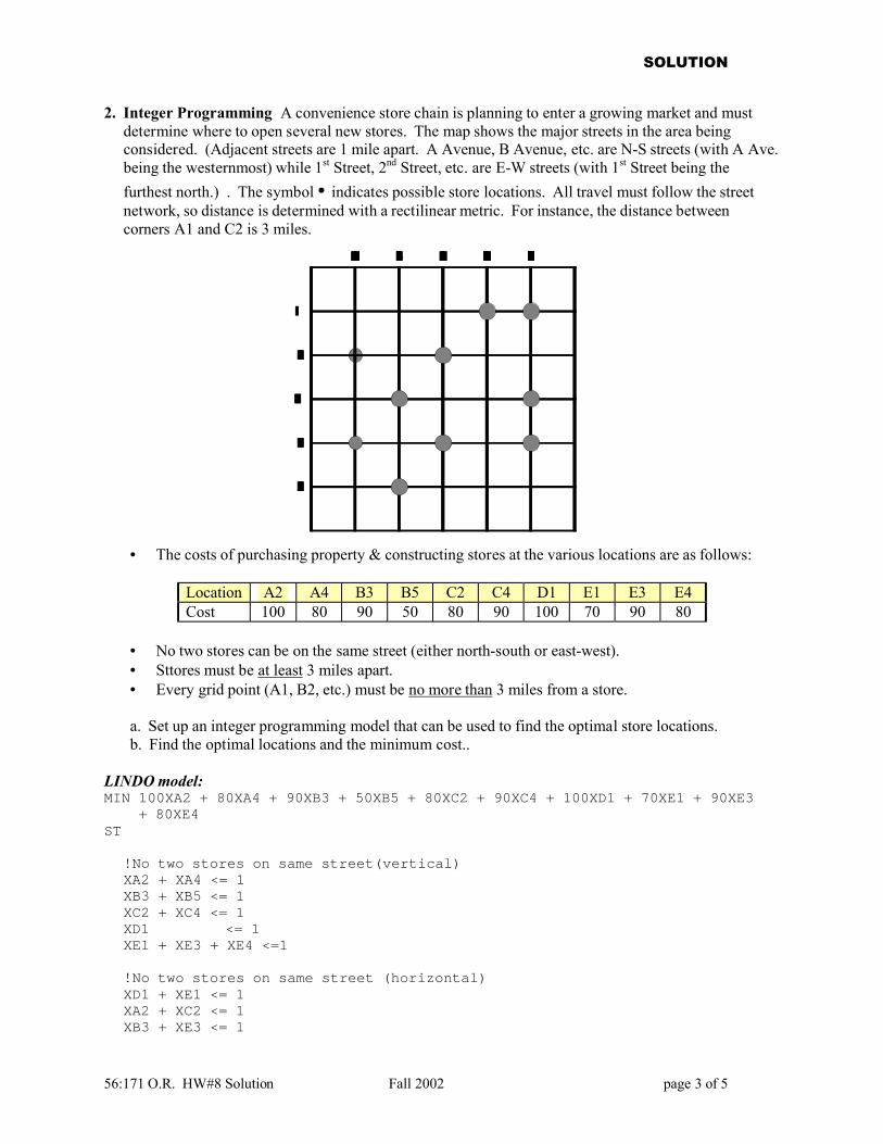
2. Integer Programming A convenience store chain is planning to enter a growing market and mustdetermine where to open several new stores. The map shows the major streets in the area beingconsidered. (Adjacent streets are 1 mile apart. A Avenue, B Avenue, etc. are N-S streets (with A Ave.being the westernmost) while 1st Street, 2nd Street, etc. are E-W streets (with 1st Street being thefurthest north.) . The symbol • indicates possible store locations. All travel must follow the streetnetwork, so distance is determined with a rectilinear metric. For instance, the distance betweencorners A1 and C2 is 3 miles.

• The costs of purchasing property & constructing stores at the various locations are as follows:

Location A2 A4 B3 B5 C2 C4 D1 E1 E3 E4Cost 100 80 90 50 80 90 100 70 90 80

• No two stores can be on the same street (either north-south or east-west).• Sttores must be at least 3 miles apart.• Every grid point (A1, B2, etc.) must be no more than 3 miles from a store.

a. Set up an integer programming model that can be used to find the optimal store locations.b. Find the optimal locations and the minimum cost..

LINDO model:MIN 100XA2 + 80XA4 + 90XB3 + 50XB5 + 80XC2 + 90XC4 + 100XD1 + 70XE1 + 90XE3

+ 80XE4ST

!No two stores on same street(vertical)XA2 + XA4 <= 1 XB3 + XB5 <= 1XC2 + XC4 <= 1XD1 <= 1XE1 + XE3 + XE4 <=1

!No two stores on same street (horizontal)XD1 + XE1 <= 1XA2 + XC2 <= 1XB3 + XE3 <= 1

SOLUTION


XA4 + XC4 + XE4 <= 1XB5 <= 1

!Store A2 3 mile constraintXA2 + XA4 <= 1XA2 + XB3 <= 1XA2 + XC2 <= 1

!Store A4 3 mile constraintXA4 + XB3 <= 1XA4 + XB5 <= 1XA4 + XC4 <= 1

!Store B3 3 mile constraintXB3 + XB5 <= 1XB3 + XC2 <= 1XB3 + XC4 <= 1

!Store B5 3 mile constraintXB5 + XC4 <= 1

!Store C2 3 mile constraintXC2 + XC4 <= 1XC2 + XD1 <= 1!XC2 + XE1 <= 1 !XC2 + XE3 <= 1

!Store C4 3 mile constraintXC4 + XE3 <= 1XC4 + XE4 <= 1

!Store D1 3 mile constraintXD1 + XE1 <= 1!XD1 + XE3 <= 1

!Store E1 3 mile constraintXE1 + XE3 <= 1!XE1 + XE4 <= 1

!Store E3 3 mile constraintXE3 + XE4 <= 1

!Grid Point 3 mile constraint

!AXA2 + XA4 + XB3 + XC2 >= 1XA2 + XA4 + XB3 + XC2 >= 1XA2 + XA4 + XB3 + XB5 + XC2 + XC4 >= 1XA2 + XA4 + XB3 + XB5 + XC4 >= 1XA2 + XA4 + XB3 + XB5 + XC4 >= 1

!BXA2 + XB3 + XC2 + XD1 + XE1 >= 1XA2 + XA4 + XB3 + XB5 + XC2 + XC4 + XD1 >= 1XA2 + XA4 + XB3 + XB5 + XC2 + XC4 + XE3 >= 1XA2 + XA4 + XB3 + XB5 + XC2 + XC4 + XE4 >= 1XA4 + XB3 + XB5 + XC4 >= 1

SOLUTION


!CXA2 + XB3 + XC2 + XC4 + XD1 + XE1 >= 1XA2 + XB3 + XC2 + XC4 + XD1 + XE1 + XE3 >= 1XA2 + XA4 + XB3 + XB5 + XC2 + XC4 + XD1 + XE3 + XE4 >= 1XA4 + XB3 + XB5 + XC2 + XC4 + XE3 + XE4 >= 1XA4 + XB3 + XB5 + XC2 + XC4 + XE4 >= 1

!DXC2 + XD1 + XE1 + XE3 >= 1XD2 + XA2 + XB3 + XC2 + XC4 + XD1 + XE1 + XE3 + XE4 >= 1XB3 + XC2 + XC4 + XD1 + XE1 + XE3 + XE5 >= 1XA4 + XB3 + XB5 + XC2 + XC4 + XD1 + XE3 + XE4 >= 1XB5 + XC4 + XE3 + XE4 >= 1

!EXC2 + XD1 + XE1 + XE3 + XE4 >= 1XE2 + XC2 + XD1 + XE1 + XE3 + XE4 >= 1XB3 + XC2 + XC4 + XB1 + XE1 + XE3 + XE4 >= 1XC4 + XE1 + XE3 + XE4 >= 1XB5 + XC4 + XE3 + XE4 >= 1

END

INT 10

Solution:OBJECTIVE FUNCTION VALUE

1) 200.0000

VARIABLE VALUE REDUCED COSTXB5 1.000000 50.000000XC2 1.000000 80.000000XE1 1.000000 70.000000

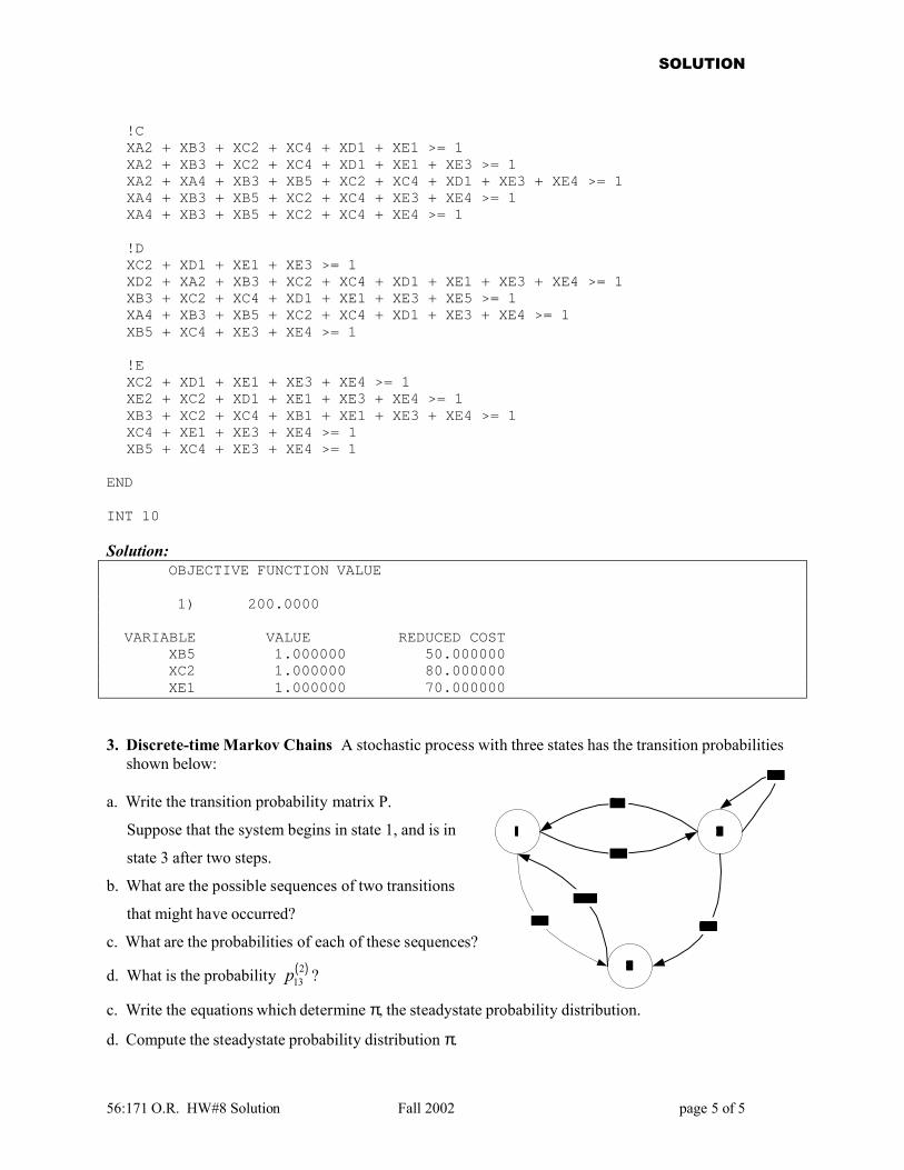
3. Discrete-time Markov Chains A stochastic process with three states has the transition probabilitiesshown below:

a. Write the transition probability matrix P.

Suppose that the system begins in state 1, and is in

state 3 after two steps.

b. What are the possible sequences of two transitions

that might have occurred?

c. What are the probabilities of each of these sequences?

d. What is the probability ( )213p ?

c. Write the equations which determine π, the steadystate probability distribution.

d. Compute the steadystate probability distribution π.

56:171 Fall 2002 Operations Research Homework Solutionsuser.engineering.uiowa.edu/~dbricker/OR_Sample_HW/OR_HW_F02_… · Fall 2002 Operations Research Homework Solutions ... Dept.

Documents