5.2 Matrix Equations - University of Utah matrix (3) below is a typical ... mate computation of the reduced row-echelon form of a matrix A. 320 ... a photo is taken.

316

5.2 Matrix Equations

Linear Equations. An m× n system of linear equations

a11x1 + a12x2 + · · ·+ a1nxn = b1,a21x1 + a22x2 + · · ·+ a2nxn = b2,

...am1x1 + am2x2 + · · ·+ amnxn = bm,

can be written as a matrix multiply equation A ~X = ~b. Let A be thematrix of coefficients aij , let ~X be the column vector of variable names

x1, . . . , xn and let ~b be the column vector with components b1, . . . , bn.Then, because equal vectors are defined by equal components,

A ~X =

a11 a12 · · · a1na21 a22 · · · a2n

...am1 am2 · · · amn

x1x2...xn

=

a11x1 + a12x2 + · · ·+ a1nxna21x1 + a22x2 + · · ·+ a2nxn

...am1x1 + am2x2 + · · ·+ amnxn

=

b1b2...bn

.

Therefore, A ~X = ~b. Conversely, a matrix equation A ~X = ~b correspondsto a set of linear algebraic equations, because of reversible steps aboveand equality of vectors.

A system of linear equations can be represented by its variable list x1,x2, . . . , xn and its augmented matrix

a11 a12 · · · a1n b1a21 a22 · · · a2n b2

...am1 am2 · · · amn bn

.(1)

The augmented matrix of system A ~X = ~b is denoted aug(A,~b) or al-ternatively < A|~b >. Given an augmented matrix C = aug(A,~b) anda variable list x1, . . . , xn, the conversion back to a linear system ofequations is made by expanding C~Y = 0, where ~Y has components x1,. . . , xn, −1. This expansion involves just dot products, therefore rapid

5.2 Matrix Equations 317

display is possible for the linear system corresponding to an augmentedmatrix. Hand work often contains the following kind of exposition:

x1 x2 · · · xna11 a12 · · · a1n b1a21 a22 · · · a2n b2

...am1 am2 · · · amn bn

(2)

In (2), a dot product is applied to the first n elements of each row, usingthe variable list written above the columns. The symbolic answer is setequal to the rightmost column’s entry, in order to recover the equations.

It is usual in homogeneous systems to not write the column of zeros, butto deal directly with A instead of aug(A,0). This convention is justifiedby arguing that the rightmost column of zeros is unchanged by swap,multiply and combination rules, which are defined for matrix equationsthe next paragraph.

Elementary Row Operations. The three operations on equationswhich produce equivalent systems can be translated directly to row op-erations on the augmented matrix for the system. The rules produceequivalent systems, that is, the three rules neither create nor destroysolutions.

Swap Two rows can be interchanged.

Multiply A row can be multiplied by multiplier m 6= 0.

Combination A multiple of one row can be added to a different row.

Documentation of Row Operations. Throughout the displaybelow, symbol s stands for source, symbol t for target, symbol m formultiplier and symbol c for constant.

Swap swap(s,t) ≡ swap rows s and t.

Multiply mult(t,m) ≡ multiply row t by m6= 0.

Combination combo(s,t,c) ≡ add c times row s to row t 6= s.

The standard for documentation is to write the notation next to thetarget row, which is the row to be changed. For swap operations, thenotation is written next to the first row that was swapped, and option-ally next to both rows. The notation was developed from early maple

notation for the corresponding operations swaprow, mulrow and addrow,appearing in the maple package linalg. In early versions of maple, an

318

additional argument A is used to reference the matrix for which the ele-mentary row operation is to be applied. For instance, addrow(A,1,3,-5)selects matrix A as the target of the combination rule, which is docu-mented in written work as combo(1,3,-5). In written work on paper,symbol A is omitted, because A is the matrix appearing on the previousline of the sequence of steps.

Maple Remarks. Versions of maple use packages to perform toolkitoperations. A short conversion table appears below.

On paper Maple with(linalg) Maple with(LinearAlgebra)

swap(s,t) swaprow(A,s,t) RowOperation(A,[t,s])

mult(t,c) mulrow(A,t,c) RowOperation(A,t,c)

combo(s,t,c) addrow(A,s,t,c) RowOperation(A,[t,s],c)

Conversion between packages can be controlled by the following functiondefinitions, which causes the maple code to be the same regardless ofwhich linear algebra package is used.6

Maple linalg

combo:=(a,s,t,c)->addrow(a,s,t,c);

swap:=(a,s,t)->swaprow(a,s,t);

mult:=(a,t,c)->mulrow(a,t,c);

Maple LinearAlgebra

combo:=(a,s,t,c)->RowOperation(a,[t,s],c);

swap:=(a,s,t)->RowOperation(a,[t,s]);

mult:=(a,t,c)->RowOperation(a,t,c);

macro(matrix=Matrix);

RREF Test. The reduced row-echelon form of a matrix, or rref, isdefined by the following requirements.

1. Zero rows appear last. Each nonzero row has first element 1, calleda leading one. The column in which the leading one appears,called a pivot column, has all other entries zero.

2. The pivot columns appear as consecutive initial columns of theidentity matrix I. Trailing columns of I might be absent.

The matrix (3) below is a typical rref which satisfies the preceding prop-erties. Displayed secondly is the reduced echelon system (4) in the vari-ables x1, . . . , x8 represented by the augmented matrix (3).

6The acronym ASTC is used for the signs of the trigonometric functions in quad-rants I through IV. The argument lists for combo, swap, mult use the same order,ASTC, memorized in trigonometry as All Students Take Calculus.


1 2 0 3 4 0 5 0 60 0 1 7 8 0 9 0 100 0 0 0 0 1 11 0 120 0 0 0 0 0 0 1 130 0 0 0 0 0 0 0 00 0 0 0 0 0 0 0 00 0 0 0 0 0 0 0 0

(3)

x1 + 2x2 + 3x4 + 4x5 + 5x7 = 6x3 + 7x4 + 8x5 + 9x7 = 10

x6 + 11x7 = 12x8 = 13

(4)

Matrix (3) is an rref and system (4) is a reduced echelon system. Theinitial 4 columns of the 7 × 7 identity matrix I appear in natural orderin matrix (3); the trailing 3 columns of I are absent.

If the rref of the augmented matrix has a leading one in the last col-umn, then the corresponding system of equations then has an equation“0 = 1” displayed, which signals an inconsistent system. It must beemphasized that an rref always exists, even if the corresponding equa-tions are inconsistent.

Elimination Method. The elimination algorithm for equations (seepage 198) has an implementation for matrices. A row is marked pro-cessed if either (1) the row is all zeros, or else (2) the row contains aleading one and all other entries in that column are zero. Otherwise, therow is called unprocessed.

1. Move each unprocessed row of zeros to the last row using swapand mark it processed.

2. Identify an unprocessed nonzero row having the least number ofleading zeros. Apply the swap rule to make this row the very firstunprocessed row. Apply the multiply rule to insure a leading one.Apply the combination rule to change to zero all other entries inthat column. The number of leading ones (lead variables) has beenincreased by one and the current column is a column of the identitymatrix. Mark the row as processed, e.g., box the leading one: 1 .

3. Repeat steps 1–2, until all rows have been processed. Then all lead-ing ones have been defined and the resulting matrix is in reducedrow-echelon form.

Computer algebra systems and computer numerical laboratories auto-mate computation of the reduced row-echelon form of a matrix A.

320

Literature calls the algorithm Gauss-Jordan elimination. Two exam-ples:

rref(0) = 0 In step 2, all rows of the zero matrix 0 are zero.No changes are made to the zero matrix.

rref(I) = I In step 2, each row has a leading one. No changesare made to the identity matrix I.

Visual RREF Test. The habit to mark pivots with a box leads to avisual test for a RREF. An illustration:

1 0 0 0 1/2

0 1 0 0 1/2

0 0 1 0 1/20 0 0 0 0

Each boxed leading one 1 appearsin a column of the identity matrix.The boxes trail downward, orderedby columns 1, 2, 3 of the identity.No 4th pivot, therefore trailing iden-tity column 4 is not used.

Frame Sequence. A sequence of swap, multiply and combinationsteps applied to a system of equations is called a frame sequence. Theviewpoint is that a camera is pointed over the shoulder of an expert whowrites the mathematics, and after the completion of each toolkit step,a photo is taken. The ordered sequence of cropped photo frames is afilmstrip or frame sequence. The First Frame displays the originalsystem and the Last Frame displays the reduced row echelon system.

The terminology applies to systems A~x = ~b represented by an augmentedmatrix C = aug(A,~b). The First Frame is C and the Last Frame isrref(C).

Documentation of frame sequence steps will use this textbook’s notation,page 317:

swap(s,t), mult(t,m), combo(s,t,c),

each written next to the target row t. During the sequence, consecutiveinitial columns of the identity, called pivot columns, are created assteps toward the rref . Trailing columns of the identity might not appear.An illustration:

Frame 1:

1 2 −1 0 11 4 −1 0 20 1 1 0 10 0 0 0 0

Original augmented matrix.

Frame 2:

1 2 −1 0 10 2 0 0 10 1 1 0 10 0 0 0 0

combo(1,2,-1)

Pivot column 1 completed.


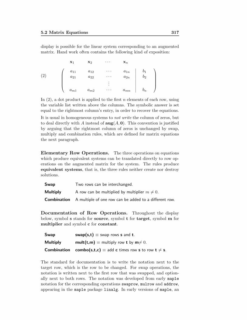
Frame 3:

1 2 −1 0 10 1 1 0 10 2 0 0 10 0 0 0 0

swap(2,3)

Frame 4:

1 2 −1 0 10 1 1 0 10 0 −2 0 −10 0 0 0 0

combo(2,3,-2)

Frame 5:

1 0 −3 0 −10 1 1 0 10 0 −2 0 −10 0 0 0 0

Pivot column 2 completed byoperation combo(2,1,-2).Back-substitution postponesthis step.

Frame 6:

1 0 −3 0 −10 1 1 0 10 0 1 0 1/20 0 0 0 0

All leading ones found.

mult(3,-1/2)

Frame 7:

1 0 −3 0 −10 1 0 0 1/20 0 1 0 1/20 0 0 0 0

combo(3,2,-1)

Zero other column 3 entries.Next, finish pivot column 3.

Last Frame:

1 0 0 0 1/20 1 0 0 1/20 0 1 0 1/20 0 0 0 0

combo(3,1,3)

rref found. Column 4 of theidentity does not appear!There is no 4th pivot column.

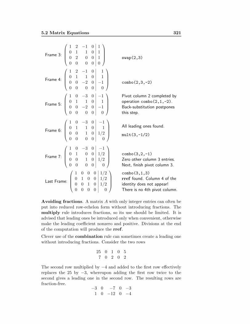
Avoiding fractions. A matrix A with only integer entries can often beput into reduced row-echelon form without introducing fractions. Themultiply rule introduces fractions, so its use should be limited. It isadvised that leading ones be introduced only when convenient, otherwisemake the leading coefficient nonzero and positive. Divisions at the endof the computation will produce the rref .

Clever use of the combination rule can sometimes create a leading onewithout introducing fractions. Consider the two rows

25 0 1 0 57 0 2 0 2

The second row multiplied by −4 and added to the first row effectivelyreplaces the 25 by −3, whereupon adding the first row twice to thesecond gives a leading one in the second row. The resulting rows arefraction-free.

−3 0 −7 0 −31 0 −12 0 −4

322

Rank and Nullity. What does it mean, if the first column of a rref isthe zero vector? It means that the corresponding variable x1 is a freevariable. In fact, every column that does not contain a leading onecorresponds to a free variable in the standard general solution of thesystem of equations. Symmetrically, each leading one identifies a pivotcolumn and corresponds to a leading variable.

The number of leading ones is the rank of the matrix, denoted rank(A).The rank cannot exceed the row dimension nor the column dimension.The column count less the number of leading ones is the nullity of thematrix, denoted nullity(A). It equals the number of free variables.

Regardless of how matrix B arises, augmented or not, we have the rela-tion

variable count = rank(B) + nullity(B).

If B = aug(A,~b) for A ~X = ~b, then the variable count n comes from ~Xand the column count of B is one more, or n+ 1. Replacing the variablecount by the column count can therefore lead to fundamental errors.

Back-substitution and efficiency. The algorithm implemented in thepreceding frame sequence is easy to learn, because the actual work is or-ganized by creating pivot columns, via swap, combination and multiply.The created pivot columns are initial columns of the identity. You areadvised to learn the algorithm in this form, but please change the algo-rithm as you become more efficient at doing the steps. See the examplesfor illustrations.

Back Substitution. Computer implementations and also hand compu-tation can be made more efficient by changing steps 2 and 3, then addingstep 4, as outlined below.

1. Move each unprocessed row of zeros to the last row using swapand mark it processed.

2a. Identify an unprocessed nonzero row having the least number ofleading zeros. Apply the swap rule to make this row the very firstunprocessed row. Apply the multiply rule to insure a leading one.Apply the combination rule to change to zero all other entries inthat column which are below the leading one.

3a. Repeat steps 1–2a, until all rows have been processed. The matrixhas all leading ones identified, a triangular shape, but it is notgenerally a RREF.

4. Back-Substitution. Identify a row with a leading one. Applythe combination rule to change to zero all other entries in thatcolumn which are above the leading one. Repeat until all rowshave been processed. The resulting matrix is a RREF.


Literature refers to step 4 as back-substitution, a process which isexactly the original elimination algorithm applied to the system createdby step 3a with reversed variable list.

Inverse Matrix. An efficient method to find the inverse B of a squarematrix A, should it happen to exist, is to form the augmented matrixC = aug(A, I) and then read off B as the package of the last n columnsof rref(C). This method is based upon the equivalence

rref(aug(A, I)) = aug(I,B) if and only if AB = I.

The next theorem aids not only in establishing this equivalence but alsoin the practical matter of testing a candidate solution for the inversematrix. The proof is delayed to page 332.

Theorem 8 (Inverse Test)If A and B are square matrices such that AB = I, then also BA = I.Therefore, only one of the equalities AB = I or BA = I is required tocheck an inverse.

Theorem 9 (The Matrix Inverse and the rref)Let A and B denote square matrices. Then

(a) If rref(aug(A, I)) = aug(I,B), then AB = BA = I and B is theinverse of A.

(b) If AB = BA = I, then rref(aug(A, I)) = aug(I,B).

(c) If rref(aug(A, I)) = aug(C,B), then C = rref(A). If C 6= I, thenA is not invertible. If C = I, then B is the inverse of A.

(d) Identity rref(A) = I holds if and only if A has an inverse.

The proof is delayed to page 333.

Finding Inverses. The method will be illustrated for the matrix

A =

1 0 10 1 −10 1 1

.Define the first frame of the sequence to be C1 = aug(A, I), then com-pute the frame sequence to rref(C1) as follows.

C1 =

1 0 1 1 0 00 1 −1 0 1 00 1 1 0 0 1

First Frame

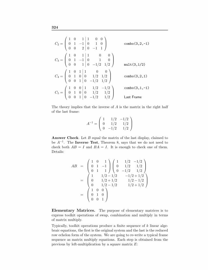
324

C2 =

1 0 1 1 0 00 1 −1 0 1 00 0 2 0 −1 1

combo(3,2,-1)

C3 =

1 0 1 1 0 00 1 −1 0 1 00 0 1 0 −1/2 1/2

mult(3,1/2)

C4 =

1 0 1 1 0 00 1 0 0 1/2 1/20 0 1 0 −1/2 1/2

combo(3,2,1)

C5 =

1 0 0 1 1/2 −1/20 1 0 0 1/2 1/20 0 1 0 −1/2 1/2

combo(3,1,-1)

Last Frame

The theory implies that the inverse of A is the matrix in the right halfof the last frame:

A−1 =

1 1/2 −1/20 1/2 1/20 −1/2 1/2

Answer Check. Let B equal the matrix of the last display, claimed tobe A−1. The Inverse Test, Theorem 8, says that we do not need tocheck both AB = I and BA = I. It is enough to check one of them.Details:

AB =

1 0 10 1 −10 1 1

1 1/2 −1/2

0 1/2 1/20 −1/2 1/2

=

1 1/2− 1/2 −1/2 + 1/20 1/2 + 1/2 1/2− 1/20 1/2− 1/2 1/2 + 1/2

=

1 0 00 1 00 0 1

Elementary Matrices. The purpose of elementary matrices is toexpress toolkit operations of swap, combination and multiply in termsof matrix multiply.

Typically, toolkit operations produce a finite sequence of k linear alge-braic equations, the first is the original system and the last is the reducedrow echelon form of the system. We are going to re-write a typical framesequence as matrix multiply equations. Each step is obtained from theprevious by left-multiplication by a square matrix E:


A ~X = ~b Original system

E1A ~X = E1~b After one toolkit step

E2E1A ~X = E2E1~b After two toolkit steps

E3E2E1A ~X = E3E2E1~b After three toolkit steps

(5)

Definition 5 (Elementary Matrix)An elementary matrix E is created from the identity matrix by applyinga single toolkit operation, that is, exactly one of the operations combi-nation, multiply or swap.

Elementary Combination Matrix. Create square matrix E by apply-ing combo(s,t,c) to the identity matrix. The result equals the identitymatrix except for the zero in row t and column s which is replaced by c.

I =

1 0 00 1 00 0 1

Identity matrix.

E =

1 0 00 1 00 c 1

Elementary combination matrix,combo(2,3,c).

Elementary Multiply Matrix. Create square matrix E by applyingmult(t,m) to the identity matrix. The result equals the identity matrixexcept the one in row t is replaced by m.

I =

1 0 00 1 00 0 1

Identity matrix.

E =

1 0 00 1 00 0 m

Elementary multiply matrix,mult(3,m).

Elementary Swap Matrix. Create square matrix E by applyingswap(s,t) to the identity matrix.

I =

1 0 00 1 00 0 1

Identity matrix.

E =

0 0 10 1 01 0 0

Elementary swap matrix,swap(1,3).

If square matrix E represents a combination, multiply or swap rule, thenthe definition of matrix multiply applied to matrix EB gives the same

326

matrix as obtained by applying the toolkit rule directly to matrix B. Thestatement is justified by experiment. See the exercises and Theorem 10.

Typical 3×3 elementary matrices (C=Combination, M=Multiply, S=Swap)can be displayed in computer algebra system maple as follows.

On Paper Maple with(linalg) Maple with(LinearAlgebra) 1 0 00 1 00 0 1

B:=diag(1,1,1); B:=IdentityMatrix(3);

combo(2,3,c) C:=addrow(B,2,3,c); C:=RowOperation(B,[3,2],c);

mult(3,m) M:=mulrow(B,3,m); M:=RowOperation(B,3,m);

swap(1,3) S:=swaprow(B,1,3); S:=RowOperation(B,[3,1]);

The reader is encouraged to write out several examples of elementarymatrices by hand or machine. Such experiments lead to the followingobservations and theorems, proofs delayed to the section end.

Constructing an Elementary Matrix E.

Combination Change a zero in the identity matrix to symbol c.

Multiply Change a one in the identity matrix to symbol m 6= 0.

Swap Interchange two rows of the identity matrix.

Constructing E−1 from an Elementary Matrix E.

Combination Change multiplier c in E to −c.

Multiply Change diagonal multiplier m 6= 0 in E to 1/m.

Swap The inverse of E is E itself.

Theorem 10 (Matrix Multiply by an Elementary Matrix)Let B1 be a given matrix of row dimension n. Select a toolkit operationcombination, multiply or swap, then apply it to matrix B1 to obtain matrixB2. Apply the identical toolkit operation to the n× n identity I to obtainelementary matrix E. Then

B2 = EB1.

Theorem 11 (Frame Sequence Identity)If C and D are any two frames in a sequence, then corresponding toolkitoperations are represented by square elementary matrices E1, E2, . . . , Ek

and the two frames C,D satisfy the matrix multiply equation

D = Ek · · ·E2E1C.


Theorem 12 (The rref and Elementary Matrices)Let A be a given matrix of row dimension n. Then there exist n × nelementary matrices E1, E2, . . . , Ek representing certain toolkit operationssuch that

rref(A) = Ek · · ·E2E1A.

Illustration. Consider the following 6-frame sequence.

A1 =

1 2 32 4 03 6 3

Frame 1, original matrix.

A2 =

1 2 30 0 −63 6 3

Frame 2, combo(1,2,-2).

A3 =

1 2 30 0 13 6 3

Frame 3, mult(2,-1/6).

A4 =

1 2 30 0 10 0 −6


A5 =

1 2 30 0 10 0 0


A6 =

1 2 00 0 10 0 0

Frame 6, combo(2,1,-3). Found rref .

The corresponding 3× 3 elementary matrices are

E1 =

1 0 0−2 1 0

0 0 1

Frame 2, combo(1,2,-2) applied to I.

E2 =

1 0 00 −1/6 00 0 1

Frame 3, mult(2,-1/6) applied to I.

E3 =

1 0 00 1 0−3 0 1


E4 =

1 0 00 1 00 −6 1


328

E5 =

1 −3 00 1 00 0 1


Because each frame of the sequence has the succinct form EB, where Eis an elementary matrix and B is the previous frame, the complete framesequence can be written as follows.

A2 = E1A1 Frame 2, E1 equals combo(1,2,-2) on I.

A3 = E2A2 Frame 3, E2 equals mult(2,-1/6) on I.




A6 = E5E4E3E2E1A1 Summary, frames 1-6. This relation isrref(A1) = E5E4E3E2E1A1, which is theresult of Theorem 12.

The summary is the equation

rref(A1) =

1−3 00 1 00 0 1

1 0 0

0 1 00−6 1

1 0 0

0 1 0−3 0 1

1 0 0

0−16 0

0 0 1

1 0 0−2 1 0

0 0 1

A1

The inverse relationship A1 = E−11 E−1

2 E−13 E−1

4 E−15 rref(A1) is formed

by the rules for constructing E−1 from elementary matrix E, page 326,the result being

A1 =

1 0 02 1 00 0 1

1 0 0

0−6 00 0 1

1 0 0

0 1 03 0 1

1 0 0

0 1 00 6 1

1 3 0

0 1 00 0 1

rref(A1)

Examples and Methods

1 Example (Identify a Reduced Row–Echelon Form) Identify the matri-ces in reduced row–echelon form using the RREF Test page 318.

A =

0 1 3 00 0 0 10 0 0 00 0 0 0

B =

1 1 3 00 0 0 10 0 0 00 0 0 0

C =

2 1 1 00 0 0 10 0 0 00 0 0 0

D =

0 1 3 00 0 0 11 0 0 00 0 0 0


Solution:

Matrix A. There are two nonzero rows, each with a leading one. The pivotcolumns are 2, 4 and they are consecutive columns of the 4× 4 identity matrix.Yes, it is a RREF.

Matrix B. Same as A but with pivot columns 1, 4. Yes, it is a RREF. Column2 is not a pivot column. The example shows that a scan for columns of theidentity is not enough.

Matrix C. Immediately not a RREF, because the leading nonzero entry inrow 1 is not a one.

Matrix D. Not a RREF. Swapping row 3 twice to bring it to row 1 will makeit a RREF. This example has pivots in columns 1, 4 but the pivot columns failto be columns 1, 2 of the identity (they are columns 3, 2).

Visual RREF Test. More experience is needed to use the visual test forRREF, but the effort is rewarded. Details are very brief. The ability to use thevisual test is learned by working examples that use the basic RREF test.

Leading ones are boxed:

A =

0 1 3 0

0 0 0 10 0 0 00 0 0 0

B =

1 1 3 0

0 0 0 10 0 0 00 0 0 0

C =

2 1 1 0

0 0 0 10 0 0 00 0 0 0

D =

0 1 3 0

0 0 0 1

1 0 0 00 0 0 0

Matrices A,B pass the visual test. Matrices C,D fail the test. Visually, we lookfor a boxed one starting on row 1. Boxes occupy consecutive rows, marchingdown and right, to make a triangular diagram.

2 Example (Reduced Row–Echelon Form) Find the reduced row–echelonform of the coefficient matrix A using the elimination method, page 319.Then solve the system.

x1 + 2x2 − x3 + x4 = 0,x1 + 3x2 − x3 + 2x4 = 0,

x2 + x4 = 0.

Solution: The coefficient matrix A and its rref are given by (details below)

A =

1 2 −1 11 3 −1 20 1 0 1

, rref(A) =

1 0 −1 −10 1 0 10 0 0 0

.

Using variable list x1, x2, x2, x4, the equivalent reduced echelon system is

x1 − x3 − x4 = 0,x2 + x4 = 0,

0 = 0.

330

which has lead variables x1, x2 and free variables x3, x4.

The last frame algorithm applies to write the standard general solution. Thisalgorithm assigns invented symbols t1, t2 to the free variables, then back-substitution is applied to the lead variables. The solution to the system is

x1 = t1 + t2,x2 = −t2,x3 = t1,x4 = t2, −∞ < t1, t2 <∞.

Details of the Elimination Method. 1∗ 2 −1 11 3 −1 20 1 0 1

The coefficient matrix A. Leading one identi-fied and marked as 1∗. 1 2 −1 1

0 1∗ 0 10 1 0 1

Apply the combination rule to zero the otherentries in column 1. Mark the row processed.Identify the next leading one, marked 1∗. 1 0 −1 −1

0 1 0 10 0 0 0

Apply the combination rule to zero the otherentries in column 2. Mark the row processed.The matrix passes the Visual RREF Test.

3 Example (Back-Substitution) Display a frame sequence which uses nu-merical efficiency ideas of back substitution, page 322, in order to find theRREF of the matrix

A =

1 2 −1 11 3 −1 20 1 0 1

,Solution: The answer for the reduced row-echelon form of matrix A is

rref(A) =

1 0 −1 00 1 0 00 0 0 1

.

Back-substitution details appear below.

Meaning of the computation. Finding a RREF is part of solving the ho-mogeneous system A ~X = ~0. The Last Frame Algorithm is used to write thegeneral solution. The algorithm requires a toolkit sequence applied to the aug-mented matrix aug(A,~0), ending in the Last Frame, which is the RREF withan added column of zeros. 1 2 −1 1

1 3 −1 20 1 0 2

The given matrix A. Identify row 1 for the firstpivot. 1 2 −1 1

0 1 0 10 1 0 2

combo(1,2,-1) applied to introduce zeros belowthe leading one in row 1.


1 2 −1 10 1 0 10 0 0 1

combo(2,3,-1) applied to introduce zeros belowthe leading one in row 2. The RREF has not yetbeen found. The matrix is triangular. 1 0 −1 −1

0 1 0 10 0 0 1

Begin back-substitution: combo(2,1,-2) appliedto introduce zeros above the leading one in row 2. 1 0 −1 0

0 1 0 00 0 0 1

Continue back-substitution: combo(3,2,-1) andcombo(3,1,1) applied to introduce zeros abovethe leading one in row 3. 1 0 −1 0

0 1 0 0

0 0 0 1

RREF Visual Test passed.This matrix is the answer.

4 Example (Answer Check a Matrix Inverse) Display the answer check de-tails for the given matrix A and its proposed inverse B.

A =

1 2 −1 10 1 0 10 0 0 10 1 1 1

, B =

1 −3 1 10 1 −1 00 −1 0 10 0 1 0

.

Solution:

Details. We apply the Inverse Test, Theorem 8, which requires one matrixmultiply:

AB =

1 2 −1 10 1 0 10 0 0 10 1 1 1

1 −3 1 10 1 −1 00 −1 0 10 0 1 0

Expect AB = I.

=

1 −3 + 2 + 1 1− 2 + 1 1− 10 1 −1 + 1 00 0 1 00 1− 1 −1 + 1 1

Multiply.

=

1 0 0 00 1 0 00 0 1 00 0 0 1

Simplify. Then AB = I.Because of Theorem 8, wedon’t check BA = I.

5 Example (Find the Inverse of a Matrix) Compute the inverse matrix of

A =

1 2 −1 10 1 0 10 0 0 10 1 1 1

.

332

Solution: The answer:

A−1 =

1 −3 1 10 1 −1 00 −1 0 10 0 1 0

.

Details. Form the augmented matrix C = aug(A, I) and compute its reducedrow-echelon form by toolkit steps.

1 2 −1 1 1 0 0 00 1 0 1 0 1 0 00 0 0 1 0 0 1 00 1 1 1 0 0 0 1

Augment I onto A.

1 2 −1 1 1 0 0 00 1 0 1 0 1 0 00 1 1 1 0 0 0 10 0 0 1 0 0 1 0

swap(3,4).

1 2 −1 1 1 0 0 00 1 0 1 0 1 0 00 0 1 0 0 −1 0 10 0 0 1 0 0 1 0

combo(2,3,-1). Triangular matrix.

1 2 −1 1 1 0 0 00 1 0 0 0 1 −1 00 0 1 0 0 −1 0 10 0 0 1 0 0 1 0

Back-substitution: combo(4,2,-1).

1 2 −1 0 1 0 −1 00 1 0 0 0 1 −1 00 0 1 0 0 −1 0 10 0 0 1 0 0 1 0

combo(4,1,-1).

1 0 −1 0 1 −2 1 00 1 0 0 0 1 −1 00 0 1 0 0 −1 0 10 0 0 1 0 0 1 0

combo(2,1,-2).

1 0 −1 0 1 −3 1 10 1 0 0 0 1 −1 00 0 1 0 0 −1 0 10 0 0 1 0 0 1 0

combo(3,1,1). Identity left, inverseright.

Details and Proofs

Proof of Theorem 8:

Assume AB = I. Let C = BA − I. We intend to show C = 0, then BA =C + I = I, as claimed.

Compute AC = ABA − A = AI − A = 0. It follows that the columns ~y of Care solutions of the homogeneous equation A~y = ~0. To complete the proof, we


show that the only solution of A~y = ~0 is ~y = ~0, because then C has all zerocolumns, which means C is the zero matrix.

First, B~u = ~0 implies ~u = I~u = AB~u = A~0 = ~0, hence B has an inverse, andthen B~x = ~y has a unique solution ~x = B−1~y.

Suppose A~y = ~0. Write ~y = B~x. Then ~x = I~x = AB~x = A~y = ~0. This implies~y = B~x = B~0 = ~0. The proof is complete.

Proof of Theorem 9:

Details for (a). Let C = aug(A, I) and assume rref(C) = aug(I,B). Solving

the n × 2n system C ~X = ~0 is equivalent to solving the system A~Y + I ~Z = ~0with n-vector unknowns ~Y and ~Z. This system has exactly the same solutionsas I ~Y + B~Z = ~0, by the equation rref(C) = aug(I,B). The latter is a

reduced echelon system with lead variables equal to the components of ~Y andfree variables equal to the components of ~Z. Multiplying by A gives A~Y +AB~Z = ~0, hence −~Z +AB~Z = ~0, or equivalently AB~Z = ~Z for every vector ~Z(because its components are free variables). Letting ~Z be a column of I showsthat AB = I. Then AB = BA = I by Theorem 8, and B is the inverse of A.

Details for (b). Assume AB = I. We prove the identity rref(aug(A, I)) =

aug(I,B). Let the system A~Y + I ~Z = ~0 have a solution ~Y , ~Z. Multiply by B

to obtain BA~Y +B~Z = ~0. Use BA = I to give ~Y +B~Z = ~0. The latter systemtherefore has ~Y , ~Z as a solution. Conversely, a solution ~Y , ~Z of ~Y +B~Z = ~0 is asolution of the system A~Y +I ~Z = ~0, because of multiplication by A. Therefore,A~Y + I ~Z = ~0 and ~Y +B~Z = ~0 are equivalent systems. The latter is in reducedrow-echelon form, and therefore rref(aug(A, I)) = aug(I,B).

Details for (c). Toolkit steps that compute rref(aug(A, I)) also computerref(A). Readers learn this fact first by working examples. Elementary matrixformulas can make the proof more transparent: see the Miscellany exercises.We conclude that rref(aug(A, I)) = aug(C,B) implies C = rref(A).

We prove C 6= I implies A is not invertible. Suppose not, then C 6= I andA is invertible. Then (b) implies aug(C,B) = rref(aug(A, I)) = aug(I,B).Comparing columns, this equation implies C = I, a contradiction.

To prove C = I implies B is the inverse of A, apply (a).

Details for (d). Assume A is invertible. We are to prove rref(A) = I. Part(b) says F = aug(A, I) satisfies rref(F ) = aug(I,B) where B is the inverse ofA. Part (c) says rref(F ) = aug(rref(A), b). Comparing matrix columns givesrref(A) = I.

Converse: assume rref(A) = I, to prove A invertible. Let F = aug(A, I), thenrref(F ) = aug(C,B) for some C,B. Part (c) says C = rref(A) = I. Part (a)says B is the inverse of A. This proves A is invertible and completes (d).

Proof of Theorem 10: It is possible to organize the proof into three cases,by considering the three possible toolkit operations. We don’t do the tediousdetails. Instead, we refer to the Elementary Matrix Multiply exercises page 335,for suitable experiments that provide the intuition needed to develop formalproof details.

Proof of Theorem 11: The idea of the proof begins with writing Frame 1as C1 = E1C, using Theorem 10. Repeat to write Frame 2 as C2 = E2C1 =

334

E2E1C. By induction, Frame k is Ck = EkCk−1 = Ek · · ·E2E1C. But Framek is matrix D in the sequence. The proof is complete.

Proof of Theorem 12: The reduced row-echelon matrix D = rref(A) pairedwith C = A imply by Theorem 11 that rref(A) = D = Ek · · ·E2E1C =Ek · · ·E2E1A. The proof is complete.

Exercises 5.2

Identify RREF. Mark the matriceswhich pass the RREF Test, page 318.Explain the failures.

1.

0 1 2 0 10 0 0 1 00 0 0 0 0

2.

0 1 0 0 00 0 1 0 30 0 0 1 2

3.

1 0 0 00 0 1 00 1 0 1

4.

1 1 4 10 0 1 00 0 0 0

Lead and Free Variables. For eachmatrix A, assume a homogeneous sys-tem A ~X = ~0 with variable list x1, . . . ,xn. List the lead and free variables.Then report the rank and nullity ofmatrix A.

5.

0 1 3 0 00 0 0 1 00 0 0 0 0

6.

0 1 0 0 00 0 1 0 30 0 0 1 2

7.

0 1 3 00 0 0 10 0 0 0

8.

1 2 3 00 0 0 10 0 0 0

9.

1 2 30 0 00 0 00 0 0

10.

1 1 00 0 10 0 0

11.

1 1 3 5 00 0 0 0 10 0 0 0 0

12.

1 2 0 3 40 0 1 1 10 0 0 0 0

13.

0 0 1 2 00 0 0 0 10 0 0 0 00 0 0 0 0

14.

0 0 0 1 10 0 0 0 00 0 0 0 00 0 0 0 0

15.

0 1 0 5 00 0 1 2 00 0 0 0 10 0 0 0 0

16.

1 0 3 0 00 1 0 1 00 0 0 0 10 0 0 0 0

Elementary Matrices. Write the 3×3elementary matrix E and its inverseE−1 for each of the following opera-tions, defined on page 317.

17. combo(1,3,-1)

18. combo(2,3,-5)

19. combo(3,2,4)


20. combo(2,1,4)

21. combo(1,2,-1)

22. combo(1,2,-e2)

23. mult(1,5)

24. mult(1,-3)

25. mult(2,5)

26. mult(2,-2)

27. mult(3,4)

28. mult(3,5)

29. mult(2,-π)

30. mult(1,e2)

31. swap(1,3)

32. swap(1,2)

33. swap(2,3)

34. swap(2,1)

35. swap(3,2)

36. swap(3,1)

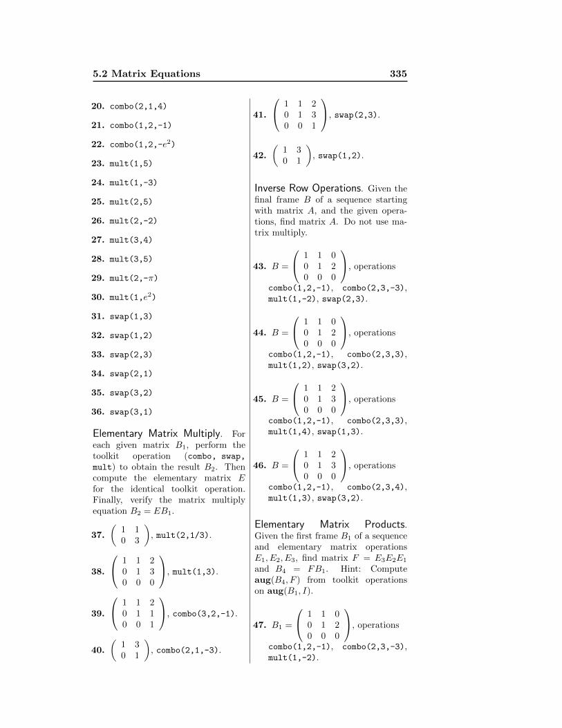
Elementary Matrix Multiply. Foreach given matrix B1, perform thetoolkit operation (combo, swap,

mult) to obtain the result B2. Thencompute the elementary matrix Efor the identical toolkit operation.Finally, verify the matrix multiplyequation B2 = EB1.

37.

(1 10 3

), mult(2,1/3).

38.

1 1 20 1 30 0 0

, mult(1,3).

39.

1 1 20 1 10 0 1

, combo(3,2,-1).

40.

(1 30 1

), combo(2,1,-3).

41.

1 1 20 1 30 0 1

, swap(2,3).

42.

(1 30 1

), swap(1,2).

Inverse Row Operations. Given thefinal frame B of a sequence startingwith matrix A, and the given opera-tions, find matrix A. Do not use ma-trix multiply.

43. B =

1 1 00 1 20 0 0

, operations

combo(1,2,-1), combo(2,3,-3),mult(1,-2), swap(2,3).

44. B =

1 1 00 1 20 0 0

, operations

combo(1,2,-1), combo(2,3,3),mult(1,2), swap(3,2).

45. B =

1 1 20 1 30 0 0

, operations


46. B =

1 1 20 1 30 0 0

, operations


Elementary Matrix Products.Given the first frame B1 of a sequenceand elementary matrix operationsE1, E2, E3, find matrix F = E3E2E1

and B4 = FB1. Hint: Computeaug(B4, F ) from toolkit operationson aug(B1, I).

47. B1 =

1 1 00 1 20 0 0

, operations

combo(1,2,-1), combo(2,3,-3),mult(1,-2).

336

48. B1 =

1 1 00 1 20 0 0

, operations

combo(1,2,-1), combo(2,3,3),swap(3,2).

49. B1 =

1 1 20 1 30 0 0

, operations

combo(1,2,-1), mult(1,4),swap(1,3).

50. B1 =

1 1 20 1 30 0 0

, operations

combo(1,2,-1), combo(2,3,4),mult(1,3).

Miscellany.

51. Justify with English sentenceswhy all possible 2×2 matrices in re-duced row-echelon form must looklike (

0 00 0

),

(1 ∗0 0

),(

0 10 0

),

(1 00 1

),

where ∗ denotes an arbitrary num-ber.

52. Display all possible 3× 3 matricesin reduced row-echelon form. Be-sides the zero matrix and the iden-tity matrix, please report five otherforms, most containing symbol ∗representing an arbitrary number.

53. Determine all possible 4×4 matri-ces in reduced row-echelon form.

54. Display a 6× 6 matrix in reducedrow-echelon form with rank 4 andonly entries of zero and one.

55. Display a 5 × 5 matrix in re-duced row-echelon form with nul-lity 2 having entries of zero, oneand two, but no other entries.

56. Display the rank and nullity of anyn× n elementary matrix.

57. Let F = aug(C,D) and let E be asquare matrix with row dimensionmatching F . Display the details forthe equality

EF = aug(EC,ED).

58. Let F = aug(C,D) and let E1, E2

be n × n matrices with n equal tothe row dimension of F . Displaythe details for the equality

E2E1F = aug(E2E1C,E2E1D).

59. Display details explaining whyrref(aug(A, I)) equals the ma-trix aug(rref(A), B), where ma-trix B = Ek · · ·E1. Symbols Ei

are elementary matrices in toolkitsteps taking aug(A, I) into re-duced row-echelon form. Sugges-tion: Use the preceding exercises.

60. Assume E1, E2 are elementarymatrices in toolkit steps takingA into reduced row-echelon form.Prove that A−1 = E2E1. In words,A−1 is found by doing the sametoolkit steps to the identity matrix.

61. Assume E1, . . . , Ek are elementarymatrices in toolkit steps takingaug(A, I) into reduced row-echelonform. Prove that A−1 = Ek · · ·E1.

62. Assume A,B are 2 × 2 matri-ces. Assume rref(aug(A,B)) =aug(I,D). Explain why the firstcolumn ~x of D is the unique solu-tion of A~x = ~b, where ~b is the firstcolumn of B.

63. Assume A,B are n × n matrices.Explain how to solve the matrixequation AX = B for matrix X us-ing the augmented matrix of A,B.

5.2 Matrix Equations - University of Utah matrix (3) below is a typical ... mate computation of the reduced row-echelon form of a matrix A. 320 ... a photo is taken.

Documents