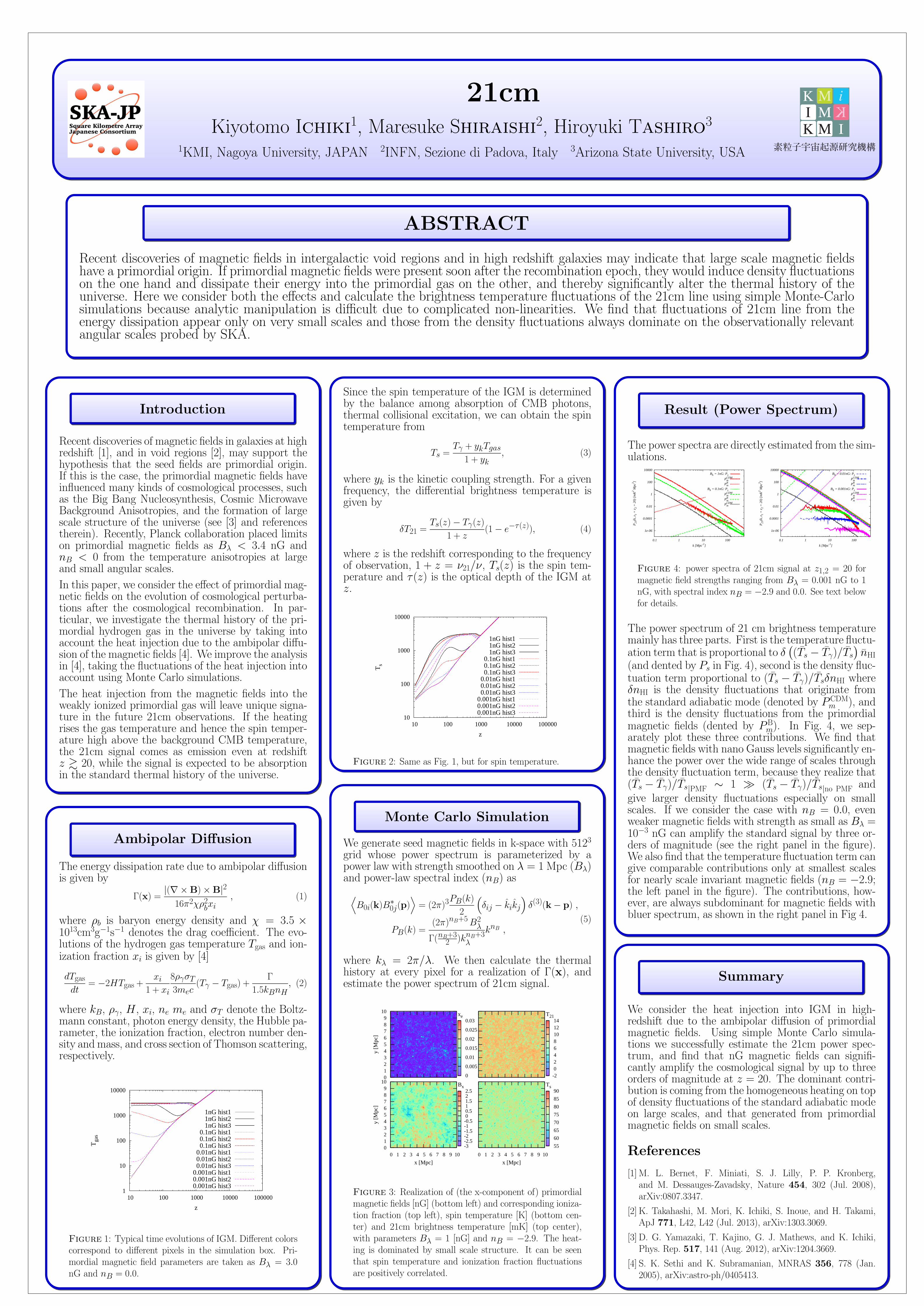
21cm Kiyotomo Ichiki 1 , Maresuke Shiraishi 2 , Hiroyuki Tashiro 3 1 KMI, Nagoya University, JAPAN 2 INFN, Sezione di Padova, Italy 3 Arizona State University, USA ABSTRACT Recent discoveries of magnetic fields in intergalactic void regions and in high redshift galaxies may indicate that large scale magnetic fields have a primordial origin. If primordial magnetic fields were present soon after the recombination epoch, they would induce density fluctuations on the one hand and dissipate their energy into the primordial gas on the other, and thereby significantly alter the thermal history of the universe. Here we consider both the effects and calculate the brightness temperature fluctuations of the 21cm line using simple Monte-Carlo simulations because analytic manipulation is difficult due to complicated non-linearities. We find that fluctuations of 21cm line from the energy dissipation appear only on very small scales and those from the density fluctuations always dominate on the observationally relevant angular scales probed by SKA. Introduction Recent discoveries of magnetic fields in galaxies at high redshift [1], and in void regions [2], may support the hypothesis that the seed fields are primordial origin. If this is the case, the primordial magnetic fields have influenced many kinds of cosmological processes, such as the Big Bang Nucleosynthesis, Cosmic Microwave Background Anisotropies, and the formation of large scale structure of the universe (see [3] and references therein). Recently, Planck collaboration placed limits on primordial magnetic fields as B λ < 3.4 nG and n B < 0 from the temperature anisotropies at large and small angular scales. In this paper, we consider the effect of primordial mag- netic fields on the evolution of cosmological perturba- tions after the cosmological recombination. In par- ticular, we investigate the thermal history of the pri- mordial hydrogen gas in the universe by taking into account the heat injection due to the ambipolar diffu- sion of the magnetic fields [4]. We improve the analysis in [4], taking the fluctuations of the heat injection into account using Monte Carlo simulations. The heat injection from the magnetic fields into the weakly ionized primordial gas will leave unique signa- ture in the future 21cm observations. If the heating rises the gas temperature and hence the spin temper- ature high above the background CMB temperature, the 21cm signal comes as emission even at redshift z 20, while the signal is expected to be absorption in the standard thermal history of the universe. Ambipolar Diffusion The energy dissipation rate due to ambipolar diffusion is given by Γ(x)= |(∇× B) × B| 2 16π 2 χρ 2 b x i , (1) where ρ b is baryon energy density and χ =3.5 × 10 13 cm 3 g −1 s −1 denotes the drag coefficient. The evo- lutions of the hydrogen gas temperature T gas and ion- ization fraction x i is given by [4] dT gas dt = −2HT gas + x i 1+ x i 8ρ γ σ T 3m e c (T γ − T gas )+ Γ 1.5k B n H , (2) where k B , ρ γ , H , x i , n e m e and σ T denote the Boltz- mann constant, photon energy density, the Hubble pa- rameter, the ionization fraction, electron number den- sity and mass, and cross section of Thomson scattering, respectively. 1 10 100 1000 10000 10 100 1000 10000 100000 T gas z 1nG hist1 1nG hist2 1nG hist3 0.1nG hist1 0.1nG hist2 0.1nG hist3 0.01nG hist1 0.01nG hist2 0.01nG hist3 0.001nG hist1 0.001nG hist2 0.001nG hist3 Figure 1: Typical time evolutions of IGM. Different colors correspond to different pixels in the simulation box. Pri- mordial magnetic field parameters are taken as B λ =3.0 nG and n B =0.0. Since the spin temperature of the IGM is determined by the balance among absorption of CMB photons, thermal collisional excitation, we can obtain the spin temperature from T s = T γ + y k T gas 1+ y k , (3) where y k is the kinetic coupling strength. For a given frequency, the differential brightness temperature is given by δT 21 = T s (z ) − T γ (z ) 1+ z (1 − e −τ (z ) ), (4) where z is the redshift corresponding to the frequency of observation, 1 + z = ν 21 /ν , T s (z ) is the spin tem- perature and τ (z ) is the optical depth of the IGM at z . 10 100 1000 10000 10 100 1000 10000 100000 T s z 1nG hist1 1nG hist2 1nG hist3 0.1nG hist1 0.1nG hist2 0.1nG hist3 0.01nG hist1 0.01nG hist2 0.01nG hist3 0.001nG hist1 0.001nG hist2 0.001nG hist3 Figure 2: Same as Fig. 1, but for spin temperature. Monte Carlo Simulation We generate seed magnetic fields in k-space with 512 3 grid whose power spectrum is parameterized by a power law with strength smoothed on λ = 1 Mpc (B λ ) and power-law spectral index (n B ) as B 0i (k)B ∗ 0j (p) = (2π ) 3 P B (k ) 2 δ ij − ˆ k i ˆ k j δ (3) (k − p) , P B (k )= (2π ) n B +5 B 2 λ Γ( n B +3 2 )k n B +3 λ k n B , (5) where k λ =2π/λ. We then calculate the thermal history at every pixel for a realization of Γ(x), and estimate the power spectrum of 21cm signal. 0 1 2 3 4 5 6 7 8 9 10 x [Mpc] 0 1 2 3 4 5 6 7 8 9 10 y [Mpc] -3 -2.5 -2 -1.5 -1 -0.5 0 0.5 1 1.5 2 2.5 B x 0 1 2 3 4 5 6 7 8 9 10 x [Mpc] 55 60 65 70 75 80 85 90 T s -2 0 2 4 6 8 10 12 14 T 21 0 1 2 3 4 5 6 7 8 9 10 y [Mpc] 0 0.005 0.01 0.015 0.02 0.025 0.03 x e Figure 3: Realization of (the x-component of) primordial magnetic fields [nG] (bottom left) and corresponding ioniza- tion fraction (top left), spin temperature [K] (bottom cen- ter) and 21cm brightness temperature [mK] (top center), with parameters B λ = 1 [nG] and n B = −2.9. The heat- ing is dominated by small scale structure. It can be seen that spin temperature and ionization fraction fluctuations are positively correlated. Result (Power Spectrum) The power spectra are directly estimated from the sim- ulations. 1e-06 0.0001 0.01 1 100 10000 0.1 1 10 100 P 21 (k, z 1 = z 2 = 20) [mK 2 Mpc 3 ] k [Mpc -1 ] B λ = 1nG: P s P CDM m P B m B λ = 0.1nG: P s P CDM m P B m P CDM m 1e-06 0.0001 0.01 1 100 10000 0.1 1 10 100 P 21 (k, z 1 = z 2 = 20) [mK 2 Mpc 3 ] k [Mpc -1 ] B λ = 0.01nG: P s P CDM m P B m B λ = 0.001nG: P s P CDM m P B m Figure 4: power spectra of 21cm signal at z 1,2 = 20 for magnetic field strengths ranging from B λ =0.001 nG to 1 nG, with spectral index n B = −2.9 and 0.0. See text below for details. The power spectrum of 21 cm brightness temperature mainly has three parts. First is the temperature fluctu- ation term that is proportional to δ ( ( ¯ T s − ¯ T γ )/ ¯ T s ) ¯ n HI (and dented by P s in Fig. 4), second is the density fluc- tuation term proportional to ( ¯ T s − ¯ T γ )/ ¯ T s δn HI where δn HI is the density fluctuations that originate from the standard adiabatic mode (denoted by P CDM m ), and third is the density fluctuations from the primordial magnetic fields (dented by P B m ). In Fig. 4, we sep- arately plot these three contributions. We find that magnetic fields with nano Gauss levels significantly en- hance the power over the wide range of scales through the density fluctuation term, because they realize that ( ¯ T s − ¯ T γ )/ ¯ T s |PMF ∼ 1 ≫ ( ¯ T s − ¯ T γ )/ ¯ T s |no PMF and give larger density fluctuations especially on small scales. If we consider the case with n B =0.0, even weaker magnetic fields with strength as small as B λ = 10 −3 nG can amplify the standard signal by three or- ders of magnitude (see the right panel in the figure). We also find that the temperature fluctuation term can give comparable contributions only at smallest scales for nearly scale invariant magnetic fields (n B = −2.9; the left panel in the figure). The contributions, how- ever, are always subdominant for magnetic fields with bluer spectrum, as shown in the right panel in Fig 4. Summary We consider the heat injection into IGM in high- redshift due to the ambipolar diffusion of primordial magnetic fields. Using simple Monte Carlo simula- tions we successfully estimate the 21cm power spec- trum, and find that nG magnetic fields can signifi- cantly amplify the cosmological signal by up to three orders of magnitude at z = 20. The dominant contri- bution is coming from the homogeneous heating on top of density fluctuations of the standard adiabatic mode on large scales, and that generated from primordial magnetic fields on small scales. References [1] M. L. Bernet, F. Miniati, S. J. Lilly, P. P. Kronberg, and M. Dessauges-Zavadsky, Nature 454, 302 (Jul. 2008), arXiv:0807.3347. [2]K. Takahashi, M. Mori, K. Ichiki, S. Inoue, and H. Takami, ApJ 771, L42, L42 (Jul. 2013), arXiv:1303.3069. [3] D. G. Yamazaki, T. Kajino, G. J. Mathews, and K. Ichiki, Phys. Rep. 517, 141 (Aug. 2012), arXiv:1204.3669. [4] S. K. Sethi and K. Subramanian, MNRAS 356, 778 (Jan. 2005), arXiv:astro-ph/0405413.

Welcome message from author
This document is posted to help you gain knowledge. Please leave a comment to let me know what you think about it! Share it to your friends and learn new things together.
Transcript
宇宙初期磁場と21cmシグナルKiyotomo Ichiki1, Maresuke Shiraishi2, Hiroyuki Tashiro3
1KMI, Nagoya University, JAPAN 2INFN, Sezione di Padova, Italy 3Arizona State University, USA
ABSTRACT
Recent discoveries of magnetic fields in intergalactic void regions and in high redshift galaxies may indicate that large scale magnetic fieldshave a primordial origin. If primordial magnetic fields were present soon after the recombination epoch, they would induce density fluctuationson the one hand and dissipate their energy into the primordial gas on the other, and thereby significantly alter the thermal history of theuniverse. Here we consider both the effects and calculate the brightness temperature fluctuations of the 21cm line using simple Monte-Carlosimulations because analytic manipulation is difficult due to complicated non-linearities. We find that fluctuations of 21cm line from theenergy dissipation appear only on very small scales and those from the density fluctuations always dominate on the observationally relevantangular scales probed by SKA.
Introduction
Recent discoveries of magnetic fields in galaxies at highredshift [1], and in void regions [2], may support thehypothesis that the seed fields are primordial origin.If this is the case, the primordial magnetic fields haveinfluenced many kinds of cosmological processes, suchas the Big Bang Nucleosynthesis, Cosmic MicrowaveBackground Anisotropies, and the formation of largescale structure of the universe (see [3] and referencestherein). Recently, Planck collaboration placed limitson primordial magnetic fields as Bλ < 3.4 nG andnB < 0 from the temperature anisotropies at largeand small angular scales.
In this paper, we consider the effect of primordial mag-netic fields on the evolution of cosmological perturba-tions after the cosmological recombination. In par-ticular, we investigate the thermal history of the pri-mordial hydrogen gas in the universe by taking intoaccount the heat injection due to the ambipolar diffu-sion of the magnetic fields [4]. We improve the analysisin [4], taking the fluctuations of the heat injection intoaccount using Monte Carlo simulations.
The heat injection from the magnetic fields into theweakly ionized primordial gas will leave unique signa-ture in the future 21cm observations. If the heatingrises the gas temperature and hence the spin temper-ature high above the background CMB temperature,the 21cm signal comes as emission even at redshiftz & 20, while the signal is expected to be absorptionin the standard thermal history of the universe.
Ambipolar Diffusion
The energy dissipation rate due to ambipolar diffusionis given by
Γ(x) =|(∇×B)×B|2
16π2χρ2bxi, (1)
where ρb is baryon energy density and χ = 3.5 ×1013cm3g−1s−1 denotes the drag coefficient. The evo-lutions of the hydrogen gas temperature Tgas and ion-ization fraction xi is given by [4]
dTgasdt
= −2HTgas +xi
1 + xi
8ργσT3mec
(Tγ − Tgas) +Γ
1.5kBnH, (2)
where kB, ργ, H , xi, ne me and σT denote the Boltz-mann constant, photon energy density, the Hubble pa-rameter, the ionization fraction, electron number den-sity and mass, and cross section of Thomson scattering,respectively.
1
10
100
1000
10000
10 100 1000 10000 100000
Tga
s
z
1nG hist11nG hist21nG hist3
0.1nG hist10.1nG hist20.1nG hist3
0.01nG hist10.01nG hist20.01nG hist3
0.001nG hist10.001nG hist20.001nG hist3
Figure 1: Typical time evolutions of IGM. Different colorscorrespond to different pixels in the simulation box. Pri-mordial magnetic field parameters are taken as Bλ = 3.0nG and nB = 0.0.
Since the spin temperature of the IGM is determinedby the balance among absorption of CMB photons,thermal collisional excitation, we can obtain the spintemperature from
Ts =Tγ + ykTgas
1 + yk, (3)
where yk is the kinetic coupling strength. For a givenfrequency, the differential brightness temperature isgiven by
δT21 =Ts(z)− Tγ(z)
1 + z(1− e−τ (z)), (4)
where z is the redshift corresponding to the frequencyof observation, 1 + z = ν21/ν, Ts(z) is the spin tem-perature and τ (z) is the optical depth of the IGM atz.
10
100
1000
10000
10 100 1000 10000 100000
Ts
z
1nG hist11nG hist21nG hist3
0.1nG hist10.1nG hist20.1nG hist3
0.01nG hist10.01nG hist20.01nG hist3
0.001nG hist10.001nG hist20.001nG hist3
Figure 2: Same as Fig. 1, but for spin temperature.
Monte Carlo Simulation
We generate seed magnetic fields in k-space with 5123
grid whose power spectrum is parameterized by apower law with strength smoothed on λ = 1 Mpc (Bλ)and power-law spectral index (nB) as
⟨
B0i(k)B∗0j(p)
⟩
= (2π)3PB(k)
2
(
δij − k̂ik̂j
)
δ(3)(k− p) ,
PB(k) =(2π)nB+5B2
λ
Γ(nB+32 )knB+3
λ
knB ,(5)
where kλ = 2π/λ. We then calculate the thermalhistory at every pixel for a realization of Γ(x), andestimate the power spectrum of 21cm signal.
0 1 2 3 4 5 6 7 8 9 10
x [Mpc]
0 1 2 3 4 5 6 7 8 9
10
y [M
pc]
-3-2.5-2-1.5-1-0.5 0 0.5 1 1.5 2 2.5
Bx
0 1 2 3 4 5 6 7 8 9 10
x [Mpc]
55
60
65
70
75
80
85
90Ts
-2 0 2 4 6 8 10 12 14
T21
0 1 2 3 4 5 6 7 8 9
10
y [M
pc]
0
0.005
0.01
0.015
0.02
0.025
0.03xe
Figure 3: Realization of (the x-component of) primordialmagnetic fields [nG] (bottom left) and corresponding ioniza-tion fraction (top left), spin temperature [K] (bottom cen-ter) and 21cm brightness temperature [mK] (top center),with parameters Bλ = 1 [nG] and nB = −2.9. The heat-ing is dominated by small scale structure. It can be seenthat spin temperature and ionization fraction fluctuationsare positively correlated.
Result (Power Spectrum)
The power spectra are directly estimated from the sim-ulations.
1e-06
0.0001
0.01
1
100
10000
0.1 1 10 100
P21
(k, z
1 =
z2
= 2
0) [
mK
2 Mpc
3 ]
k [Mpc-1]
Bλ = 1nG: Ps
PCDMm
PBm
Bλ = 0.1nG: Ps
PCDMm
PBm
PCDMm
1e-06
0.0001
0.01
1
100
10000
0.1 1 10 100
P21
(k, z
1 =
z2
= 2
0) [
mK
2 Mpc
3 ]
k [Mpc-1]
Bλ = 0.01nG: Ps
PCDMm
PBm
Bλ = 0.001nG: Ps
PCDMm
PBm
Figure 4: power spectra of 21cm signal at z1,2 = 20 formagnetic field strengths ranging from Bλ = 0.001 nG to 1nG, with spectral index nB = −2.9 and 0.0. See text belowfor details.
The power spectrum of 21 cm brightness temperaturemainly has three parts. First is the temperature fluctu-ation term that is proportional to δ
(
(T̄s − T̄γ)/T̄s
)
n̄HI
(and dented by Ps in Fig. 4), second is the density fluc-tuation term proportional to (T̄s − T̄γ)/T̄sδnHI whereδnHI is the density fluctuations that originate fromthe standard adiabatic mode (denoted by PCDM
m ), andthird is the density fluctuations from the primordialmagnetic fields (dented by PB
m). In Fig. 4, we sep-arately plot these three contributions. We find thatmagnetic fields with nano Gauss levels significantly en-hance the power over the wide range of scales throughthe density fluctuation term, because they realize that(T̄s − T̄γ)/T̄s|PMF ∼ 1 ≫ (T̄s − T̄γ)/T̄s|no PMF andgive larger density fluctuations especially on smallscales. If we consider the case with nB = 0.0, evenweaker magnetic fields with strength as small as Bλ =10−3 nG can amplify the standard signal by three or-ders of magnitude (see the right panel in the figure).We also find that the temperature fluctuation term cangive comparable contributions only at smallest scalesfor nearly scale invariant magnetic fields (nB = −2.9;the left panel in the figure). The contributions, how-ever, are always subdominant for magnetic fields withbluer spectrum, as shown in the right panel in Fig 4.
Summary
We consider the heat injection into IGM in high-redshift due to the ambipolar diffusion of primordialmagnetic fields. Using simple Monte Carlo simula-tions we successfully estimate the 21cm power spec-trum, and find that nG magnetic fields can signifi-cantly amplify the cosmological signal by up to threeorders of magnitude at z = 20. The dominant contri-bution is coming from the homogeneous heating on topof density fluctuations of the standard adiabatic modeon large scales, and that generated from primordialmagnetic fields on small scales.
References
[1] M. L. Bernet, F. Miniati, S. J. Lilly, P. P. Kronberg,and M. Dessauges-Zavadsky, Nature 454, 302 (Jul. 2008),arXiv:0807.3347.
[2] K. Takahashi, M. Mori, K. Ichiki, S. Inoue, and H. Takami,ApJ 771, L42, L42 (Jul. 2013), arXiv:1303.3069.
[3] D. G. Yamazaki, T. Kajino, G. J. Mathews, and K. Ichiki,Phys. Rep. 517, 141 (Aug. 2012), arXiv:1204.3669.
[4] S. K. Sethi and K. Subramanian, MNRAS 356, 778 (Jan.2005), arXiv:astro-ph/0405413.
Related Documents


![Esoterism hist2 sommar11 [Skrivskyddad] [Kompatibilitetsläge]/PPThomas2.pdf · 2011. 11. 4. · Microsoft PowerPoint - Esoterism hist2 sommar11 [Skrivskyddad] [Kompatibilitetsläge]](https://static.cupdf.com/doc/110x72/6042be0a6ec8624d5362e79b/esoterism-hist2-sommar11-skrivskyddad-kompatibilitetslge-2011-11-4.jpg)