5. the arctic - American Meteorological Society

5. THE ARCTICa. Overview—J. Richter-Menge and J. T. Mathis

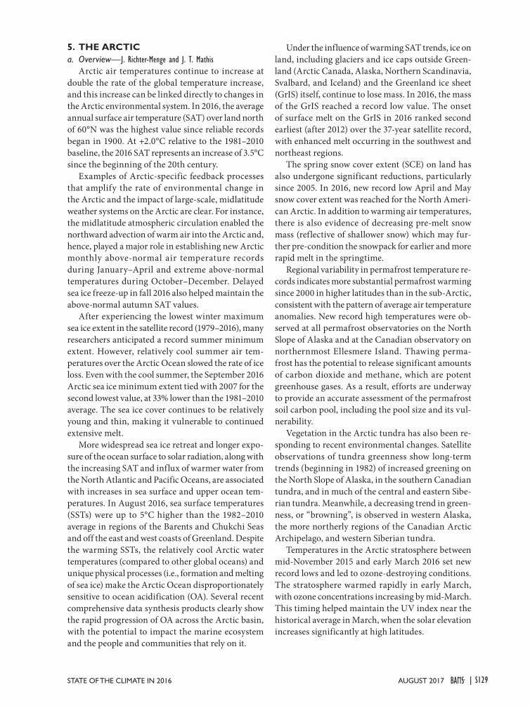
Arctic air temperatures continue to increase at double the rate of the global temperature increase, and this increase can be linked directly to changes in the Arctic environmental system. In 2016, the average annual surface air temperature (SAT) over land north of 60°N was the highest value since reliable records began in 1900. At +2.0°C relative to the 1981–2010 baseline, the 2016 SAT represents an increase of 3.5°C since the beginning of the 20th century.

Examples of Arctic-specific feedback processes that amplify the rate of environmental change in the Arctic and the impact of large-scale, midlatitude weather systems on the Arctic are clear. For instance, the midlatitude atmospheric circulation enabled the northward advection of warm air into the Arctic and, hence, played a major role in establishing new Arctic monthly above-normal air temperature records during January–April and extreme above-normal temperatures during October–December. Delayed sea ice freeze-up in fall 2016 also helped maintain the above-normal autumn SAT values.

After experiencing the lowest winter maximum sea ice extent in the satellite record (1979–2016), many researchers anticipated a record summer minimum extent. However, relatively cool summer air tem-peratures over the Arctic Ocean slowed the rate of ice loss. Even with the cool summer, the September 2016 Arctic sea ice minimum extent tied with 2007 for the second lowest value, at 33% lower than the 1981–2010 average. The sea ice cover continues to be relatively young and thin, making it vulnerable to continued extensive melt.

More widespread sea ice retreat and longer expo-sure of the ocean surface to solar radiation, along with the increasing SAT and influx of warmer water from the North Atlantic and Pacific Oceans, are associated with increases in sea surface and upper ocean tem-peratures. In August 2016, sea surface temperatures (SSTs) were up to 5°C higher than the 1982–2010 average in regions of the Barents and Chukchi Seas and off the east and west coasts of Greenland. Despite the warming SSTs, the relatively cool Arctic water temperatures (compared to other global oceans) and unique physical processes (i.e., formation and melting of sea ice) make the Arctic Ocean disproportionately sensitive to ocean acidification (OA). Several recent comprehensive data synthesis products clearly show the rapid progression of OA across the Arctic basin, with the potential to impact the marine ecosystem and the people and communities that rely on it.

Under the influence of warming SAT trends, ice on land, including glaciers and ice caps outside Green-land (Arctic Canada, Alaska, Northern Scandinavia, Svalbard, and Iceland) and the Greenland ice sheet (GrIS) itself, continue to lose mass. In 2016, the mass of the GrIS reached a record low value. The onset of surface melt on the GrIS in 2016 ranked second earliest (after 2012) over the 37-year satellite record, with enhanced melt occurring in the southwest and northeast regions.

The spring snow cover extent (SCE) on land has also undergone significant reductions, particularly since 2005. In 2016, new record low April and May snow cover extent was reached for the North Ameri-can Arctic. In addition to warming air temperatures, there is also evidence of decreasing pre-melt snow mass (reflective of shallower snow) which may fur-ther pre-condition the snowpack for earlier and more rapid melt in the springtime.

Regional variability in permafrost temperature re-cords indicates more substantial permafrost warming since 2000 in higher latitudes than in the sub-Arctic, consistent with the pattern of average air temperature anomalies. New record high temperatures were ob-served at all permafrost observatories on the North Slope of Alaska and at the Canadian observatory on northernmost Ellesmere Island. Thawing perma-frost has the potential to release significant amounts of carbon dioxide and methane, which are potent greenhouse gases. As a result, efforts are underway to provide an accurate assessment of the permafrost soil carbon pool, including the pool size and its vul-nerability.

Vegetation in the Arctic tundra has also been re-sponding to recent environmental changes. Satellite observations of tundra greenness show long-term trends (beginning in 1982) of increased greening on the North Slope of Alaska, in the southern Canadian tundra, and in much of the central and eastern Sibe-rian tundra. Meanwhile, a decreasing trend in green-ness, or “browning”, is observed in western Alaska, the more northerly regions of the Canadian Arctic Archipelago, and western Siberian tundra.

Temperatures in the Arctic stratosphere between mid-November 2015 and early March 2016 set new record lows and led to ozone-destroying conditions. The stratosphere warmed rapidly in early March, with ozone concentrations increasing by mid-March. This timing helped maintain the UV index near the historical average in March, when the solar elevation increases significantly at high latitudes.

AUGUST 2017STATE OF THE CLIMATE IN 2016 | S129

The Arctic chapter describes a range of observa-tions of essential climate variables (ECV; Bojinski et al. 2014) and other physical environmental variables, encompassing the atmosphere, ocean, and land in the Arctic and sub-Arctic. When possible, the current standard reference period (defined as 1981–2010 by the World Meteorological Organization and national agencies such as NOAA) is used for calculating cli-mate normals (averages) and anomalies. However, it cannot be used for all the variables described, as some organizations choose not to use 1981–2010 and many Arctic observational records post-date 1981.

While the use of different base periods to describe the state of different elements of the Arctic environ-ment is unavoidable, it does not alter the fact that rapid change is occurring throughout the Arctic en-vironmental system. There are numerous and diverse signals indicating that the Arctic environment con-tinues to be influenced by long-term upward trends in air temperature, modulated by natural variability in regional and seasonal anomalies. The accelera-tion of many of these signals, the interdependency of the physical and biological elements of the Arctic system, and the growing recognition that the Arctic is an integral part of the larger Earth system are increasing the pressure for more effective and timely communication of these scientific observations to diverse users. A key to meeting this challenging goal is to more directly convey the synthesis of observa-tions across disciplinary boundaries in an effort to better highlight Arctic system change.

b. Surface air temperature— J . Over land, E. Hanna , I. Hanssen-Bauer, S.-J. Kim, J. E. Walsh, M. Wang, U. S. Bhatt, and R. L. ThomanThe average annual surface air temperature

(SAT) anomaly for 2016 for land stations north of

60°N was +2.0°C, relative to the 1981–2010 average value (Fig. 5.1). This marks a new high for the record starting in 1900, and is a significant increase over the previous highest value of +1.2°C, which was observed in 2007, 2011, and 2015. Average global annual tem-peratures also showed record values in 2015 and 2016. Currently, the Arctic is warming at more than twice the rate of lower latitudes.

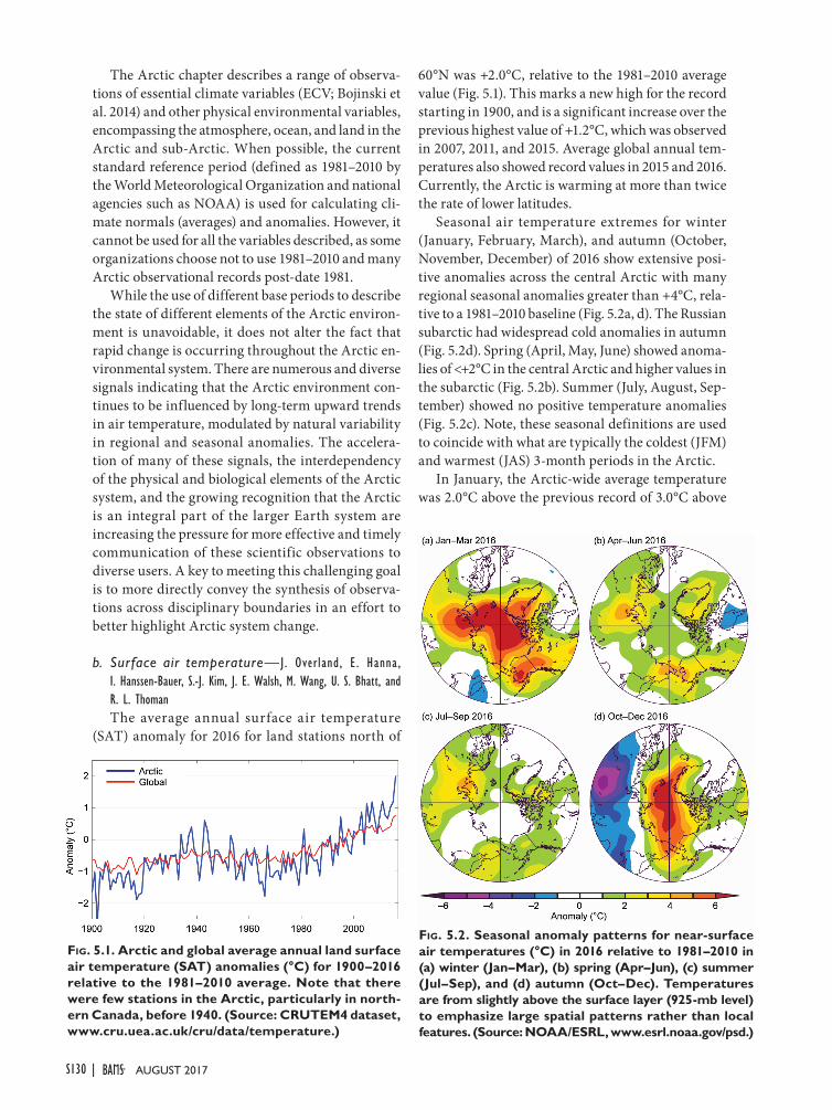
Seasonal air temperature extremes for winter (January, February, March), and autumn (October, November, December) of 2016 show extensive posi-tive anomalies across the central Arctic with many regional seasonal anomalies greater than +4°C, rela-tive to a 1981–2010 baseline (Fig. 5.2a, d). The Russian subarctic had widespread cold anomalies in autumn (Fig. 5.2d). Spring (April, May, June) showed anoma-lies of <+2°C in the central Arctic and higher values in the subarctic (Fig. 5.2b). Summer (July, August, Sep-tember) showed no positive temperature anomalies (Fig. 5.2c). Note, these seasonal definitions are used to coincide with what are typically the coldest (JFM) and warmest (JAS) 3-month periods in the Arctic.

In January, the Arctic-wide average temperature was 2.0°C above the previous record of 3.0°C above

Fig. 5.1. Arctic and global average annual land surface air temperature (SAT) anomalies (°C) for 1900–2016 relative to the 1981–2010 average. Note that there were few stations in the Arctic, particularly in north-ern Canada, before 1940. (Source: CRUTEM4 dataset, www.cru.uea.ac.uk/cru/data/temperature.)

Fig. 5.2. Seasonal anomaly patterns for near-surface air temperatures (°C) in 2016 relative to 1981–2010 in (a) winter (Jan–Mar), (b) spring (Apr–Jun), (c) summer (Jul–Sep), and (d) autumn (Oct–Dec). Temperatures are from slightly above the surface layer (925-mb level) to emphasize large spatial patterns rather than local features. (Source: NOAA/ESRL, www.esrl.noaa.gov/psd.)

AUGUST 2017|S130

the 1981–2010 normal. Some local January observa-tions were in excess of 7°C above normal (Overland and Wang 2016). Near-record high temperatures were experienced in some northern Greenland locations. From January through April, Alaska had record high minimum temperatures in all subregions and record high temperature maximums for most subregions (Walsh et al. 2017).

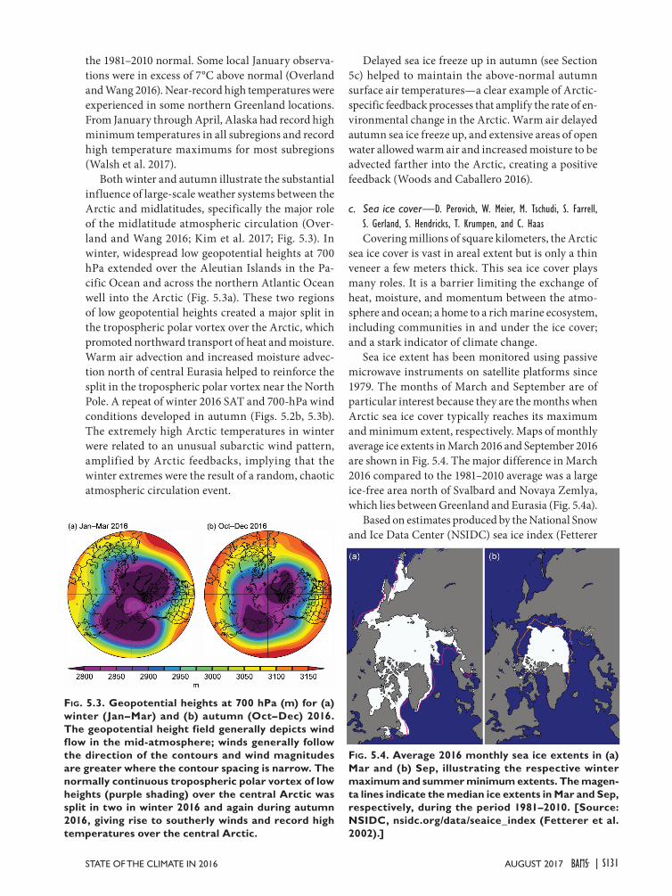
Both winter and autumn illustrate the substantial influence of large-scale weather systems between the Arctic and midlatitudes, specifically the major role of the midlatitude atmospheric circulation (Over-land and Wang 2016; Kim et al. 2017; Fig. 5.3). In winter, widespread low geopotential heights at 700 hPa extended over the Aleutian Islands in the Pa-cific Ocean and across the northern Atlantic Ocean well into the Arctic (Fig. 5.3a). These two regions of low geopotential heights created a major split in the tropospheric polar vortex over the Arctic, which promoted northward transport of heat and moisture. Warm air advection and increased moisture advec-tion north of central Eurasia helped to reinforce the split in the tropospheric polar vortex near the North Pole. A repeat of winter 2016 SAT and 700-hPa wind conditions developed in autumn (Figs. 5.2b, 5.3b). The extremely high Arctic temperatures in winter were related to an unusual subarctic wind pattern, amplified by Arctic feedbacks, implying that the winter extremes were the result of a random, chaotic atmospheric circulation event.

Delayed sea ice freeze up in autumn (see Section 5c) helped to maintain the above-normal autumn surface air temperatures—a clear example of Arctic-specific feedback processes that amplify the rate of en-vironmental change in the Arctic. Warm air delayed autumn sea ice freeze up, and extensive areas of open water allowed warm air and increased moisture to be advected farther into the Arctic, creating a positive feedback (Woods and Caballero 2016).

c. Sea ice cover—D. Perovich, W. Meier, M. Tschudi, S. Farrell, S. Gerland, S. Hendricks, T. Krumpen, and C. HaasCovering millions of square kilometers, the Arctic

sea ice cover is vast in areal extent but is only a thin veneer a few meters thick. This sea ice cover plays many roles. It is a barrier limiting the exchange of heat, moisture, and momentum between the atmo-sphere and ocean; a home to a rich marine ecosystem, including communities in and under the ice cover; and a stark indicator of climate change.

Sea ice extent has been monitored using passive microwave instruments on satellite platforms since 1979. The months of March and September are of particular interest because they are the months when Arctic sea ice cover typically reaches its maximum and minimum extent, respectively. Maps of monthly average ice extents in March 2016 and September 2016 are shown in Fig. 5.4. The major difference in March 2016 compared to the 1981–2010 average was a large ice-free area north of Svalbard and Novaya Zemlya, which lies between Greenland and Eurasia (Fig. 5.4a).

Based on estimates produced by the National Snow and Ice Data Center (NSIDC) sea ice index (Fetterer

Fig. 5.3. Geopotential heights at 700 hPa (m) for (a) winter (Jan–Mar) and (b) autumn (Oct–Dec) 2016. The geopotential height field generally depicts wind flow in the mid-atmosphere; winds generally follow the direction of the contours and wind magnitudes are greater where the contour spacing is narrow. The normally continuous tropospheric polar vortex of low heights (purple shading) over the central Arctic was split in two in winter 2016 and again during autumn 2016, giving rise to southerly winds and record high temperatures over the central Arctic.

Fig. 5.4. Average 2016 monthly sea ice extents in (a) Mar and (b) Sep, illustrating the respective winter maximum and summer minimum extents. The magen-ta lines indicate the median ice extents in Mar and Sep, respectively, during the period 1981–2010. [Source: NSIDC, nsidc.org/data/seaice_index (Fetterer et al. 2002).]


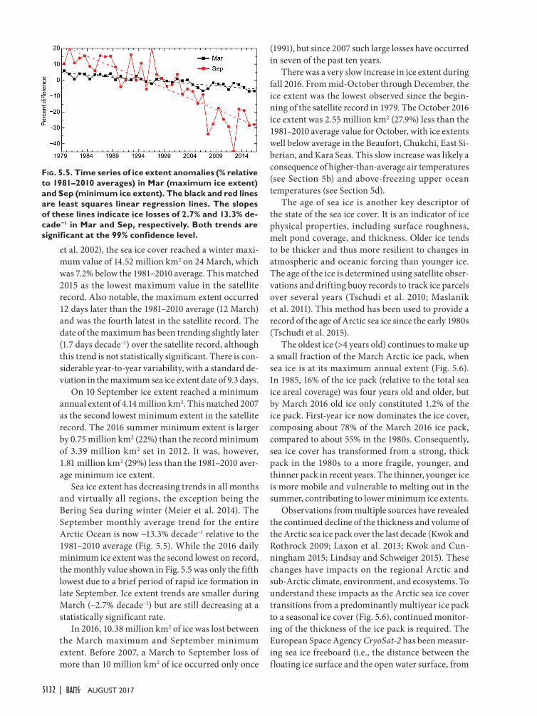
et al. 2002), the sea ice cover reached a winter maxi-mum value of 14.52 million km2 on 24 March, which was 7.2% below the 1981–2010 average. This matched 2015 as the lowest maximum value in the satellite record. Also notable, the maximum extent occurred 12 days later than the 1981–2010 average (12 March) and was the fourth latest in the satellite record. The date of the maximum has been trending slightly later (1.7 days decade−1) over the satellite record, although this trend is not statistically significant. There is con-siderable year-to-year variability, with a standard de-viation in the maximum sea ice extent date of 9.3 days.

On 10 September ice extent reached a minimum annual extent of 4.14 million km2. This matched 2007 as the second lowest minimum extent in the satellite record. The 2016 summer minimum extent is larger by 0.75 million km2 (22%) than the record minimum of 3.39 million km2 set in 2012. It was, however, 1.81 million km2 (29%) less than the 1981–2010 aver-age minimum ice extent.

Sea ice extent has decreasing trends in all months and virtually all regions, the exception being the Bering Sea during winter (Meier et al. 2014). The September monthly average trend for the entire Arctic Ocean is now −13.3% decade−1 relative to the 1981–2010 average (Fig. 5.5). While the 2016 daily minimum ice extent was the second lowest on record, the monthly value shown in Fig. 5.5 was only the fifth lowest due to a brief period of rapid ice formation in late September. Ice extent trends are smaller during March (−2.7% decade−1) but are still decreasing at a statistically significant rate.

In 2016, 10.38 million km2 of ice was lost between the March maximum and September minimum extent. Before 2007, a March to September loss of more than 10 million km2 of ice occurred only once

(1991), but since 2007 such large losses have occurred in seven of the past ten years.

There was a very slow increase in ice extent during fall 2016. From mid-October through December, the ice extent was the lowest observed since the begin-ning of the satellite record in 1979. The October 2016 ice extent was 2.55 million km2 (27.9%) less than the 1981–2010 average value for October, with ice extents well below average in the Beaufort, Chukchi, East Si-berian, and Kara Seas. This slow increase was likely a consequence of higher-than-average air temperatures (see Section 5b) and above-freezing upper ocean temperatures (see Section 5d).

The age of sea ice is another key descriptor of the state of the sea ice cover. It is an indicator of ice physical properties, including surface roughness, melt pond coverage, and thickness. Older ice tends to be thicker and thus more resilient to changes in atmospheric and oceanic forcing than younger ice. The age of the ice is determined using satellite obser-vations and drifting buoy records to track ice parcels over several years (Tschudi et al. 2010; Maslanik et al. 2011). This method has been used to provide a record of the age of Arctic sea ice since the early 1980s (Tschudi et al. 2015).

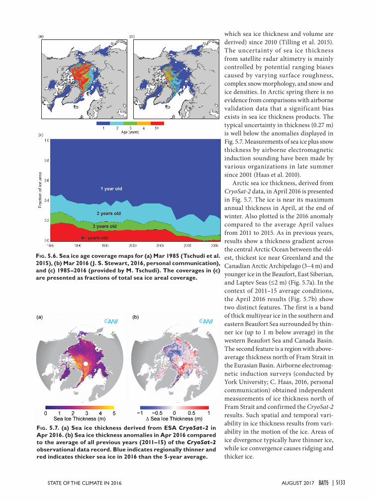
The oldest ice (>4 years old) continues to make up a small fraction of the March Arctic ice pack, when sea ice is at its maximum annual extent (Fig. 5.6). In 1985, 16% of the ice pack (relative to the total sea ice areal coverage) was four years old and older, but by March 2016 old ice only constituted 1.2% of the ice pack. First-year ice now dominates the ice cover, composing about 78% of the March 2016 ice pack, compared to about 55% in the 1980s. Consequently, sea ice cover has transformed from a strong, thick pack in the 1980s to a more fragile, younger, and thinner pack in recent years. The thinner, younger ice is more mobile and vulnerable to melting out in the summer, contributing to lower minimum ice extents.

Observations from multiple sources have revealed the continued decline of the thickness and volume of the Arctic sea ice pack over the last decade (Kwok and Rothrock 2009; Laxon et al. 2013; Kwok and Cun-ningham 2015; Lindsay and Schweiger 2015). These changes have impacts on the regional Arctic and sub-Arctic climate, environment, and ecosystems. To understand these impacts as the Arctic sea ice cover transitions from a predominantly multiyear ice pack to a seasonal ice cover (Fig. 5.6), continued monitor-ing of the thickness of the ice pack is required. The European Space Agency CryoSat-2 has been measur-ing sea ice freeboard (i.e., the distance between the floating ice surface and the open water surface, from

Fig. 5.5. Time series of ice extent anomalies (% relative to 1981–2010 averages) in Mar (maximum ice extent) and Sep (minimum ice extent). The black and red lines are least squares linear regression lines. The slopes of these lines indicate ice losses of 2.7% and 13.3% de-cade−1 in Mar and Sep, respectively. Both trends are significant at the 99% confidence level.

AUGUST 2017|S132

which sea ice thickness and volume are derived) since 2010 (Tilling et al. 2015). The uncertainty of sea ice thickness from satellite radar altimetry is mainly controlled by potential ranging biases caused by varying surface roughness, complex snow morphology, and snow and ice densities. In Arctic spring there is no evidence from comparisons with airborne validation data that a significant bias exists in sea ice thickness products. The typical uncertainty in thickness (0.27 m) is well below the anomalies displayed in Fig. 5.7. Measurements of sea ice plus snow thickness by airborne electromagnetic induction sounding have been made by various organizations in late summer since 2001 (Haas et al. 2010).

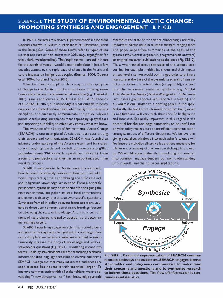
Arctic sea ice thickness, derived from CryoSat-2 data, in April 2016 is presented in Fig. 5.7. The ice is near its maximum annual thickness in April, at the end of winter. Also plotted is the 2016 anomaly compared to the average April values from 2011 to 2015. As in previous years, results show a thickness gradient across the central Arctic Ocean between the old-est, thickest ice near Greenland and the Canadian Arctic Archipelago (3–4 m) and younger ice in the Beaufort, East Siberian, and Laptev Seas (≤2 m) (Fig. 5.7a). In the context of 2011–15 average conditions, the April 2016 results (Fig. 5.7b) show two distinct features. The first is a band of thick multiyear ice in the southern and eastern Beaufort Sea surrounded by thin-ner ice (up to 1 m below average) in the western Beaufort Sea and Canada Basin. The second feature is a region with above-average thickness north of Fram Strait in the Eurasian Basin. Airborne electromag-netic induction surveys (conducted by York University; C. Haas, 2016, personal communication) obtained independent measurements of ice thickness north of Fram Strait and confirmed the CryoSat-2 results. Such spatial and temporal vari-ability in ice thickness results from vari-ability in the motion of the ice. Areas of ice divergence typically have thinner ice, while ice convergence causes ridging and thicker ice.

Fig. 5.6. Sea ice age coverage maps for (a) Mar 1985 (Tschudi et al. 2015), (b) Mar 2016 (J. S. Stewart, 2016, personal communication), and (c) 1985–2016 (provided by M. Tschudi). The coverages in (c) are presented as fractions of total sea ice areal coverage.

Fig. 5.7. (a) Sea ice thickness derived from ESA CryoSat-2 in Apr 2016. (b) Sea ice thickness anomalies in Apr 2016 compared to the average of all previous years (2011–15) of the CryoSat-2 observational data record. Blue indicates regionally thinner and red indicates thicker sea ice in 2016 than the 5-year average.


In 1979, I learned a few dozen Yupik words for sea ice from Conrad Oozeva, a Native hunter from St. Lawrence Island in the Bering Sea. Some of those terms refer to types of sea ice that are rare or non-existent in 2016 (e.g., tagneghneq for thick, dark, weathered ice). That Yupik terms—probably in use for thousands of years—would become obsolete in just a few decades attests to the rapid pace of change in the Arctic and to the impacts on Indigenous peoples (Berman 2004; Oozeva et al. 2004; Ford and Pearce 2010).

Scientists in many disciplines also recognize the rapid pace of change in the Arctic and the importance of being more timely and effective in conveying what we know (e.g., Post et al. 2013; Francis and Vavrus 2015; Grosse et al. 2016; Tedesco et al. 2016c). Further, our knowledge is most valuable to policy makers and affected communities when we synthesize across disciplines and succinctly communicate the policy-relevant points. Accelerating our science means speeding up syntheses and improving our ability to effectively convey what we know.

The evolution of the Study of Environmental Arctic Change (SEARCH) is one example of Arctic scientists accelerating their science and communication. SEARCH was founded to advance understanding of the Arctic system and its trajec-tory through synthesis and modeling (www.arcus.org/files /page/documents/19437/search_openletter_1997.pdf). From a scientific perspective, synthesis is an important step in an iterative process.

SEARCH and many in the Arctic research community have become increasingly convinced, however, that addi-tional important syntheses combining scientific research and indigenous knowledge are needed. From a scientific perspective, synthesis may be important for designing the next experiment, but policy makers, local communities, and others look to syntheses to answer specific questions. Syntheses framed in policy-relevant forms are more valu-able to these user communities than are framings focused on advancing the state of knowledge. And, in this environ-ment of rapid change, the policy questions are becoming increasingly urgent.

SEARCH now brings together scientists, stakeholders, and government agencies to synthesize knowledge from many disciplines—these syntheses are intended to simul-taneously increase the body of knowledge and address stakeholder questions (Fig. SB5.1). Translating science into forms usable by stakeholders calls for translating technical information into language accessible to diverse audiences. SEARCH recognizes that many interested audiences are sophisticated but not facile with technical jargon. To improve communication with all stakeholders, we are de-veloping “knowledge pyramids.” Each knowledge pyramid

SIDEBAR 5.1: THE STUDY OF ENVIRONMENTAL ARCTIC CHANGE: PROMOTING SYNTHESIS AND ENGAGEMENT—B. P. KELLY

assembles the state of the science concerning a societally important Arctic issue in multiple formats ranging from one-page, jargon-free summaries at the apex of the pyramid (www.arcus.org/search-program/arctic-answers) to original research publications at the base (Fig. SB5.2). Thus, when asked about the state of the science con-cerning, for example, melting ice sheets and their impact on sea level rise, we would point a geologist to primary literature at the base of the pyramid; a scientist from an-other discipline to a review article (midpyramid); a science journalist to a more condensed synthesis [e.g., NOAA Arctic Report Card essay (Richter-Menge et al. 2016); www .arctic.noaa.gov/Report-Card/Report-Card-2016]; and a Congressional staffer to a briefing paper in the apex. Naturally, the level at which someone enters the pyramid is not fixed and will vary with their specific background and interests. Especially important in this regard is the potential for the one-page summaries to be useful not only for policy makers but also for efficient communication among scientists of different disciplines. We believe that giving specialists windows into each other’s science will facilitate the multidisciplinary collaborations necessary for a fuller understanding of environmental change in the Arc-tic. We would argue further that translating our research into common language deepens our own understanding of our results and their broader implications.

Fig. SB5.1. Graphical representation of SEARCH commu-nication pathways and audiences. SEARCH engages diverse stakeholder and indigenous communities to understand their concerns and questions and to synthesize research to inform those questions. The flow of information is con-tinuous and iterative.

AUGUST 2017|S134

d. Sea surface temperature—M.-L. TimmermansSummer sea surface temperatures (SST) in the

Arctic Ocean are set mainly by absorption of solar radiation into the surface layer. In the Barents and Chukchi Seas, there is an additional contribution from advection of warm water from the North At-lantic and Pacific Oceans, respectively (for a recent assessment of this in the Chukchi Sea, see Serreze et al. 2016). Solar warming of the ocean surface layer is influenced by the distribution of sea ice (with more solar warming in ice-free regions), cloud cover, water color, and upper-ocean stratification. River influxes influence the latter two. SST data presented here are from the NOAA Optimum Interpolation (OI) SST Version 2 product (OISSTv2), which is a blend of in situ and satellite measurements (Reynolds et al. 2002, 2007). Compared to in situ temperature measure-ments, the OISSTv2 product shows average correla-tions of about 80%, with an overall cold SST bias of −0.02°C (Stroh et al. 2015).

August SSTs provide the most appropriate repre-sentation of Arctic Ocean summer SSTs, because they are not affected by the cooling and subsequent sea ice growth that typically takes place in the latter half of September. Average SSTs in August 2016 in ice-free

regions ranged from ~0°C in some regions to around +7° to +8°C in the Chukchi Sea and eastern Baffin Bay off the west coast of Greenland, and up to +11°C in the Barents Sea (Fig. 5.8a). Compared to the 1982–2010 August average (note the monthly SST record begins in December 1981), most boundary regions and mar-ginal seas of the Arctic had anomalously warm SSTs

Fig. SB5.2. Knowledge pyramids answer policy-relevant questions about the Arctic environment in a series of web-based products. Briefs are supported by documents of increasing detail in lower tiers of the pyramids.

We also appreciate and honor the valuable information found in the differences between scientific and indigenous perceptions of the Arctic. When Conrad Oozeva used numer-

ous Yupik words to describe sea ice, which I would have referred to using a single term, he drew my attention to differences in ice characteristics that I had over-looked.

The communities of St. Law-rence Island, like communities across the Arctic, are facing ex-tremely rapid changes, some of which may make obsolete certain terms in their language. Such cul-tural losses may challenge those communities, but Conrad advised young people to draw informa-tion from various sources—to synthesize—an approach likely to enhance the resilience of their

communities. The scientific community can also benefit from Conrad’s advice to think across disciplines and his example of translating his knowledge for diverse audiences.

Fig. 5.8. (a) Average SST (°C) in Aug 2016. White shading is the Aug 2016 average sea ice extent, and gray contours indicate the 10°C SST isotherm. (b) SST anomalies (°C) in Aug 2016 relative to the Aug 1982–2010 average. White shading is the Aug 2016 average ice extent and the black line indicates the median ice edge for Aug 1982–2010 average.


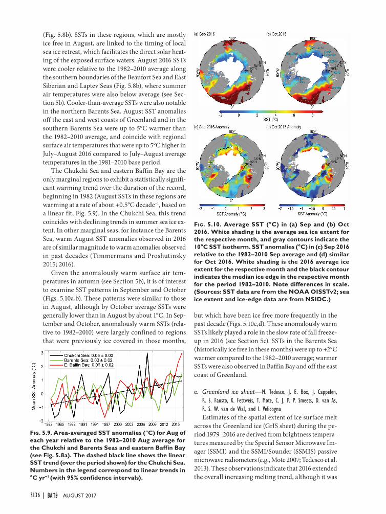
(Fig. 5.8b). SSTs in these regions, which are mostly ice free in August, are linked to the timing of local sea ice retreat, which facilitates the direct solar heat-ing of the exposed surface waters. August 2016 SSTs were cooler relative to the 1982–2010 average along the southern boundaries of the Beaufort Sea and East Siberian and Laptev Seas (Fig. 5.8b), where summer air temperatures were also below average (see Sec-tion 5b). Cooler-than-average SSTs were also notable in the northern Barents Sea. August SST anomalies off the east and west coasts of Greenland and in the southern Barents Sea were up to 5°C warmer than the 1982–2010 average, and coincide with regional surface air temperatures that were up to 5°C higher in July–August 2016 compared to July–August average temperatures in the 1981–2010 base period.

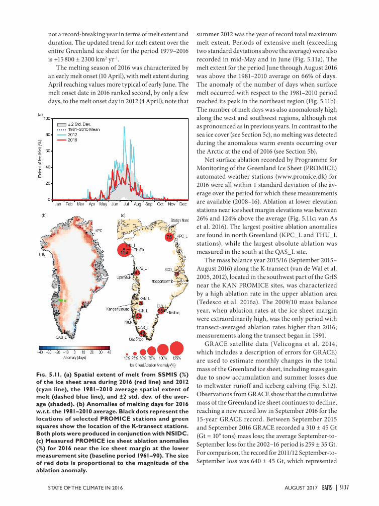
The Chukchi Sea and eastern Baffin Bay are the only marginal regions to exhibit a statistically signifi-cant warming trend over the duration of the record, beginning in 1982 (August SSTs in these regions are warming at a rate of about +0.5°C decade−1, based on a linear fit; Fig. 5.9). In the Chukchi Sea, this trend coincides with declining trends in summer sea ice ex-tent. In other marginal seas, for instance the Barents Sea, warm August SST anomalies observed in 2016 are of similar magnitude to warm anomalies observed in past decades (Timmermans and Proshutinsky 2015; 2016).

Given the anomalously warm surface air tem-peratures in autumn (see Section 5b), it is of interest to examine SST patterns in September and October (Figs. 5.10a,b). These patterns were similar to those in August, although by October average SSTs were generally lower than in August by about 1°C. In Sep-tember and October, anomalously warm SSTs (rela-tive to 1982–2010) were largely confined to regions that were previously ice covered in those months,

but which have been ice free more frequently in the past decade (Figs. 5.10c,d). These anomalously warm SSTs likely played a role in the slow rate of fall freeze-up in 2016 (see Section 5c). SSTs in the Barents Sea (historically ice free in these months) were up to +2°C warmer compared to the 1982–2010 average; warmer SSTs were also observed in Baffin Bay and off the east coast of Greenland.

e. Greenland ice sheet—M. Tedesco, J. E. Box, J. Cappelen, R. S. Fausto, X. Fettweis, T. Mote, C. J. P. P. Smeets, D. van As, R. S. W. van de Wal, and I. Velicogna Estimates of the spatial extent of ice surface melt

across the Greenland ice (GrIS sheet) during the pe-riod 1979–2016 are derived from brightness tempera-tures measured by the Special Sensor Microwave Im-ager (SSMI) and the SSMI/Sounder (SSMIS) passive microwave radiometers (e.g., Mote 2007; Tedesco et al. 2013). These observations indicate that 2016 extended the overall increasing melting trend, although it was

Fig. 5.10. Average SST (°C) in (a) Sep and (b) Oct 2016. White shading is the average sea ice extent for the respective month, and gray contours indicate the 10°C SST isotherm. SST anomalies (°C) in (c) Sep 2016 relative to the 1982–2010 Sep average and (d) similar for Oct 2016. White shading is the 2016 average ice extent for the respective month and the black contour indicates the median ice edge in the respective month for the period 1982–2010. Note differences in scale. (Sources: SST data are from the NOAA OISSTv2; sea ice extent and ice-edge data are from NSIDC.)

Fig. 5.9. Area-averaged SST anomalies (°C) for Aug of each year relative to the 1982–2010 Aug average for the Chukchi and Barents Seas and eastern Baffin Bay (see Fig. 5.8a). The dashed black line shows the linear SST trend (over the period shown) for the Chukchi Sea. Numbers in the legend correspond to linear trends in °C yr−1 (with 95% confidence intervals).

AUGUST 2017|S136

not a record-breaking year in terms of melt extent and duration. The updated trend for melt extent over the entire Greenland ice sheet for the period 1979–2016 is +15 800 ± 2300 km2 yr−1.

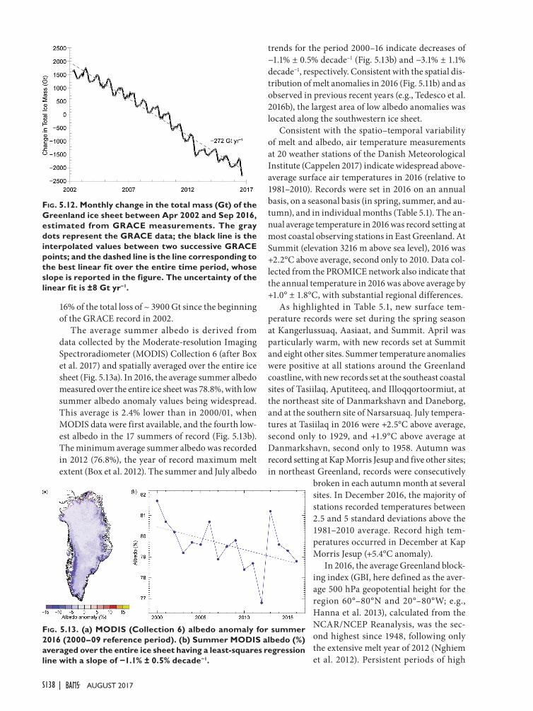
The melting season of 2016 was characterized by an early melt onset (10 April), with melt extent during April reaching values more typical of early June. The melt onset date in 2016 ranked second, by only a few days, to the melt onset day in 2012 (4 April); note that

summer 2012 was the year of record total maximum melt extent. Periods of extensive melt (exceeding two standard deviations above the average) were also recorded in mid-May and in June (Fig. 5.11a). The melt extent for the period June through August 2016 was above the 1981–2010 average on 66% of days. The anomaly of the number of days when surface melt occurred with respect to the 1981–2010 period reached its peak in the northeast region (Fig. 5.11b). The number of melt days was also anomalously high along the west and southwest regions, although not as pronounced as in previous years. In contrast to the sea ice cover (see Section 5c), no melting was detected during the anomalous warm events occurring over the Arctic at the end of 2016 (see Section 5b).

Net surface ablation recorded by Programme for Monitoring of the Greenland Ice Sheet (PROMICE) automated weather stations (www.promice.dk) for 2016 were all within 1 standard deviation of the av-erage over the period for which these measurements are available (2008–16). Ablation at lower elevation stations near ice sheet margin elevations was between 26% and 124% above the average (Fig. 5.11c; van As et al. 2016). The largest positive ablation anomalies are found in north Greenland (KPC_L and THU_L stations), while the largest absolute ablation was measured in the south at the QAS_L site.

The mass balance year 2015/16 (September 2015–August 2016) along the K-transect (van de Wal et al. 2005, 2012), located in the southwest part of the GrIS near the KAN PROMICE sites, was characterized by a high ablation rate in the upper ablation area (Tedesco et al. 2016a). The 2009/10 mass balance year, when ablation rates at the ice sheet margin were extraordinarily high, was the only period with transect-averaged ablation rates higher than 2016; measurements along the transect began in 1991.

GRACE satellite data (Velicogna et al. 2014, which includes a description of errors for GRACE) are used to estimate monthly changes in the total mass of the Greenland ice sheet, including mass gain due to snow accumulation and summer losses due to meltwater runoff and iceberg calving (Fig. 5.12). Observations from GRACE show that the cumulative mass of the Greenland ice sheet continues to decline, reaching a new record low in September 2016 for the 15-year GRACE record. Between September 2015 and September 2016 GRACE recorded a 310 ± 45 Gt (Gt = 109 tons) mass loss; the average September-to-September loss for the 2002–16 period is 259 ± 35 Gt. For comparison, the record for 2011/12 September-to-September loss was 640 ± 45 Gt, which represented

Fig. 5.11. (a) Spatial extent of melt from SSMIS (%) of the ice sheet area during 2016 (red line) and 2012 (cyan line), the 1981–2010 average spatial extent of melt (dashed blue line), and ±2 std. dev. of the aver-age (shaded). (b) Anomalies of melting days for 2016 w.r.t. the 1981–2010 average. Black dots represent the locations of selected PROMICE stations and green squares show the location of the K-transect stations. Both plots were produced in conjunction with NSIDC. (c) Measured PROMICE ice sheet ablation anomalies (%) for 2016 near the ice sheet margin at the lower measurement site (baseline period 1961–90). The size of red dots is proportional to the magnitude of the ablation anomaly.


16% of the total loss of ~ 3900 Gt since the beginning of the GRACE record in 2002.

The average summer albedo is derived from data collected by the Moderate-resolution Imaging Spectroradiometer (MODIS) Collection 6 (after Box et al. 2017) and spatially averaged over the entire ice sheet (Fig. 5.13a). In 2016, the average summer albedo measured over the entire ice sheet was 78.8%, with low summer albedo anomaly values being widespread. This average is 2.4% lower than in 2000/01, when MODIS data were first available, and the fourth low-est albedo in the 17 summers of record (Fig. 5.13b). The minimum average summer albedo was recorded in 2012 (76.8%), the year of record maximum melt extent (Box et al. 2012). The summer and July albedo

trends for the period 2000–16 indicate decreases of −1.1% ± 0.5% decade−1 (Fig. 5.13b) and −3.1% ± 1.1% decade−1, respectively. Consistent with the spatial dis-tribution of melt anomalies in 2016 (Fig. 5.11b) and as observed in previous recent years (e.g., Tedesco et al. 2016b), the largest area of low albedo anomalies was located along the southwestern ice sheet.

Consistent with the spatio–temporal variability of melt and albedo, air temperature measurements at 20 weather stations of the Danish Meteorological Institute (Cappelen 2017) indicate widespread above-average surface air temperatures in 2016 (relative to 1981–2010). Records were set in 2016 on an annual basis, on a seasonal basis (in spring, summer, and au-tumn), and in individual months (Table 5.1). The an-nual average temperature in 2016 was record setting at most coastal observing stations in East Greenland. At Summit (elevation 3216 m above sea level), 2016 was +2.2°C above average, second only to 2010. Data col-lected from the PROMICE network also indicate that the annual temperature in 2016 was above average by +1.0° ± 1.8°C, with substantial regional differences.

As highlighted in Table 5.1, new surface tem-perature records were set during the spring season at Kangerlussuaq, Aasiaat, and Summit. April was particularly warm, with new records set at Summit and eight other sites. Summer temperature anomalies were positive at all stations around the Greenland coastline, with new records set at the southeast coastal sites of Tasiilaq, Aputiteeq, and Illoqqortoormiut, at the northeast site of Danmarkshavn and Daneborg, and at the southern site of Narsarsuaq. July tempera-tures at Tasiilaq in 2016 were +2.5°C above average, second only to 1929, and +1.9°C above average at Danmarkshavn, second only to 1958. Autumn was record setting at Kap Morris Jesup and five other sites; in northeast Greenland, records were consecutively

broken in each autumn month at several sites. In December 2016, the majority of stations recorded temperatures between 2.5 and 5 standard deviations above the 1981–2010 average. Record high tem-peratures occurred in December at Kap Morris Jesup (+5.4°C anomaly).

In 2016, the average Greenland block-ing index (GBI, here defined as the aver-age 500 hPa geopotential height for the region 60°–80°N and 20°–80°W; e.g., Hanna et al. 2013), calculated from the NCAR/NCEP Reanalysis, was the sec-ond highest since 1948, following only the extensive melt year of 2012 (Nghiem et al. 2012). Persistent periods of high

Fig. 5.13. (a) MODIS (Collection 6) albedo anomaly for summer 2016 (2000–09 reference period). (b) Summer MODIS albedo (%) averaged over the entire ice sheet having a least-squares regression line with a slope of −1.1% ± 0.5% decade−1.

Fig. 5.12. Monthly change in the total mass (Gt) of the Greenland ice sheet between Apr 2002 and Sep 2016, estimated from GRACE measurements. The gray dots represent the GRACE data; the black line is the interpolated values between two successive GRACE points; and the dashed line is the line corresponding to the best linear fit over the entire time period, whose slope is reported in the figure. The uncertainty of the linear fit is ±8 Gt yr−1.

AUGUST 2017|S138

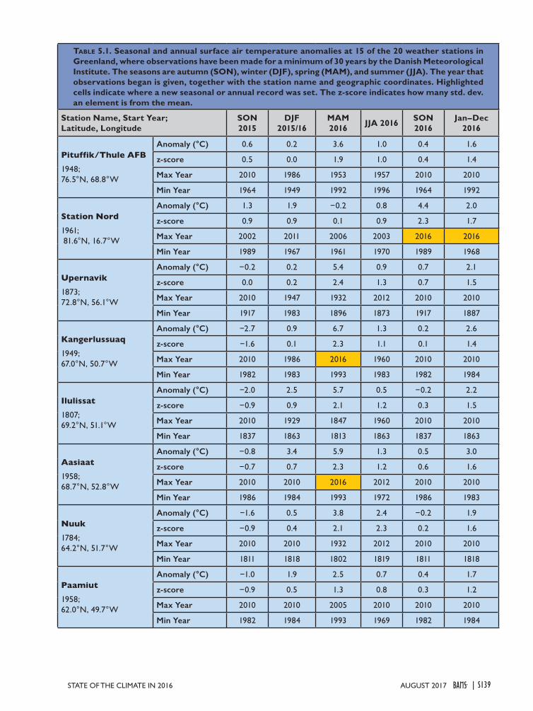
Table 5.1. Seasonal and annual surface air temperature anomalies at 15 of the 20 weather stations in Greenland, where observations have been made for a minimum of 30 years by the Danish Meteorological Institute. The seasons are autumn (SON), winter (DJF), spring (MAM), and summer (JJA). The year that observations began is given, together with the station name and geographic coordinates. Highlighted cells indicate where a new seasonal or annual record was set. The z-score indicates how many std. dev. an element is from the mean.

Station Name, Start Year; Latitude, Longitude

SON 2015

DJF 2015/16

MAM 2016 JJA 2016 SON

2016Jan–Dec

2016

Pituffik/Thule AFB1948; 76.5°N, 68.8°W

Anomaly (°C) 0.6 0.2 3.6 1.0 0.4 1.6

z-score 0.5 0.0 1.9 1.0 0.4 1.4

Max Year 2010 1986 1953 1957 2010 2010

Min Year 1964 1949 1992 1996 1964 1992

Station Nord1961; 81.6°N, 16.7°W

Anomaly (°C) 1.3 1.9 −0.2 0.8 4.4 2.0

z-score 0.9 0.9 0.1 0.9 2.3 1.7

Max Year 2002 2011 2006 2003 2016 2016

Min Year 1989 1967 1961 1970 1989 1968

Upernavik1873; 72.8°N, 56.1°W

Anomaly (°C) −0.2 0.2 5.4 0.9 0.7 2.1

z-score 0.0 0.2 2.4 1.3 0.7 1.5

Max Year 2010 1947 1932 2012 2010 2010

Min Year 1917 1983 1896 1873 1917 1887

Kangerlussuaq1949; 67.0°N, 50.7°W

Anomaly (°C) −2.7 0.9 6.7 1.3 0.2 2.6

z-score −1.6 0.1 2.3 1.1 0.1 1.4

Max Year 2010 1986 2016 1960 2010 2010

Min Year 1982 1983 1993 1983 1982 1984

Ilulissat1807; 69.2°N, 51.1°W

Anomaly (°C) −2.0 2.5 5.7 0.5 −0.2 2.2

z-score −0.9 0.9 2.1 1.2 0.3 1.5

Max Year 2010 1929 1847 1960 2010 2010

Min Year 1837 1863 1813 1863 1837 1863

Aasiaat1958; 68.7°N, 52.8°W

Anomaly (°C) −0.8 3.4 5.9 1.3 0.5 3.0

z-score −0.7 0.7 2.3 1.2 0.6 1.6

Max Year 2010 2010 2016 2012 2010 2010

Min Year 1986 1984 1993 1972 1986 1983

Nuuk1784; 64.2°N, 51.7°W

Anomaly (°C) −1.6 0.5 3.8 2.4 −0.2 1.9

z-score −0.9 0.4 2.1 2.3 0.2 1.6

Max Year 2010 2010 1932 2012 2010 2010

Min Year 1811 1818 1802 1819 1811 1818

Paamiut1958; 62.0°N, 49.7°W

Anomaly (°C) −1.0 1.9 2.5 0.7 0.4 1.7

z-score −0.9 0.5 1.3 0.8 0.3 1.2

Max Year 2010 2010 2005 2010 2010 2010

Min Year 1982 1984 1993 1969 1982 1984


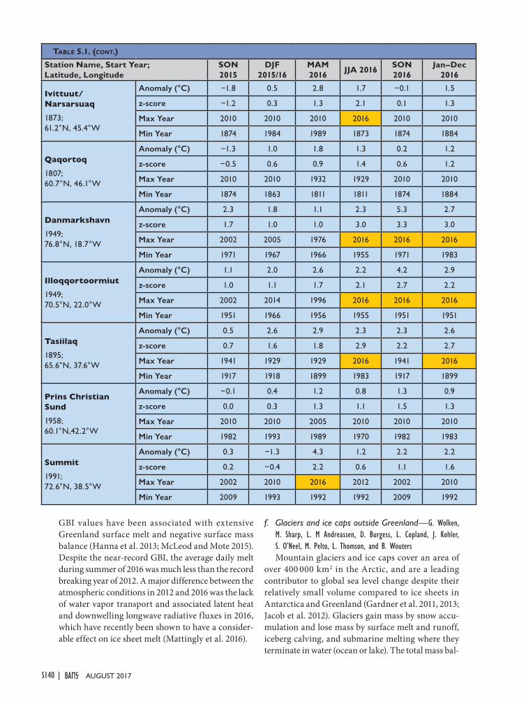
GBI values have been associated with extensive Greenland surface melt and negative surface mass balance (Hanna et al. 2013; McLeod and Mote 2015). Despite the near-record GBI, the average daily melt during summer of 2016 was much less than the record breaking year of 2012. A major difference between the atmospheric conditions in 2012 and 2016 was the lack of water vapor transport and associated latent heat and downwelling longwave radiative fluxes in 2016, which have recently been shown to have a consider-able effect on ice sheet melt (Mattingly et al. 2016).

f. Glaciers and ice caps outside Greenland—G. Wolken, M. Sharp, L. M Andreassen, D. Burgess, L. Copland, J. Kohler, S. O’Neel, M. Pelto, L. Thomson, and B. WoutersMountain glaciers and ice caps cover an area of

over 400 000 km2 in the Arctic, and are a leading contributor to global sea level change despite their relatively small volume compared to ice sheets in Antarctica and Greenland (Gardner et al. 2011, 2013; Jacob et al. 2012). Glaciers gain mass by snow accu-mulation and lose mass by surface melt and runoff, iceberg calving, and submarine melting where they terminate in water (ocean or lake). The total mass bal-

Table 5.1. (cont.)

Station Name, Start Year; Latitude, Longitude

SON 2015

DJF 2015/16

MAM 2016 JJA 2016 SON

2016Jan–Dec

2016

Ivittuut/ Narsarsuaq1873; 61.2°N, 45.4°W

Anomaly (°C) −1.8 0.5 2.8 1.7 −0.1 1.5

z-score −1.2 0.3 1.3 2.1 0.1 1.3

Max Year 2010 2010 2010 2016 2010 2010

Min Year 1874 1984 1989 1873 1874 1884

Qaqortoq1807; 60.7°N, 46.1°W

Anomaly (°C) −1.3 1.0 1.8 1.3 0.2 1.2

z-score −0.5 0.6 0.9 1.4 0.6 1.2

Max Year 2010 2010 1932 1929 2010 2010

Min Year 1874 1863 1811 1811 1874 1884

Danmarkshavn1949; 76.8°N, 18.7°W

Anomaly (°C) 2.3 1.8 1.1 2.3 5.3 2.7

z-score 1.7 1.0 1.0 3.0 3.3 3.0

Max Year 2002 2005 1976 2016 2016 2016

Min Year 1971 1967 1966 1955 1971 1983

Illoqqortoormiut1949; 70.5°N, 22.0°W

Anomaly (°C) 1.1 2.0 2.6 2.2 4.2 2.9

z-score 1.0 1.1 1.7 2.1 2.7 2.2

Max Year 2002 2014 1996 2016 2016 2016

Min Year 1951 1966 1956 1955 1951 1951

Tasiilaq1895; 65.6°N, 37.6°W

Anomaly (°C) 0.5 2.6 2.9 2.3 2.3 2.6

z-score 0.7 1.6 1.8 2.9 2.2 2.7

Max Year 1941 1929 1929 2016 1941 2016

Min Year 1917 1918 1899 1983 1917 1899

Prins Christian Sund1958; 60.1°N,42.2°W

Anomaly (°C) −0.1 0.4 1.2 0.8 1.3 0.9

z-score 0.0 0.3 1.3 1.1 1.5 1.3

Max Year 2010 2010 2005 2010 2010 2010

Min Year 1982 1993 1989 1970 1982 1983

Summit1991; 72.6°N, 38.5°W

Anomaly (°C) 0.3 −1.3 4.3 1.2 2.2 2.2

z-score 0.2 −0.4 2.2 0.6 1.1 1.6

Max Year 2002 2010 2016 2012 2002 2010

Min Year 2009 1993 1992 1992 2009 1992

AUGUST 2017|S140

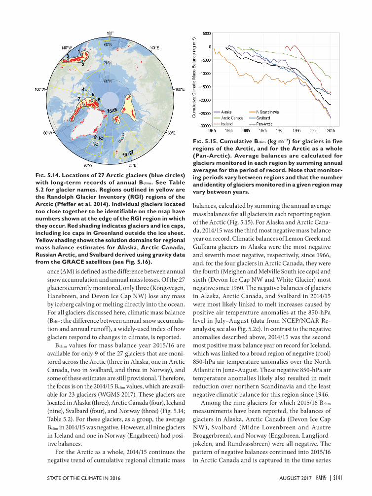
ance (ΔM) is defined as the difference between annual snow accumulation and annual mass losses. Of the 27 glaciers currently monitored, only three (Kongsvegen, Hansbreen, and Devon Ice Cap NW) lose any mass by iceberg calving or melting directly into the ocean. For all glaciers discussed here, climatic mass balance (Bclim; the difference between annual snow accumula-tion and annual runoff), a widely-used index of how glaciers respond to changes in climate, is reported.

Bclim values for mass balance year 2015/16 are available for only 9 of the 27 glaciers that are moni-tored across the Arctic (three in Alaska, one in Arctic Canada, two in Svalbard, and three in Norway), and some of these estimates are still provisional. Therefore, the focus is on the 2014/15 Bclim values, which are avail-able for 23 glaciers (WGMS 2017). These glaciers are located in Alaska (three), Arctic Canada (four), Iceland (nine), Svalbard (four), and Norway (three) (Fig. 5.14; Table 5.2). For these glaciers, as a group, the average Bclim in 2014/15 was negative. However, all nine glaciers in Iceland and one in Norway (Engabreen) had posi-tive balances.

For the Arctic as a whole, 2014/15 continues the negative trend of cumulative regional climatic mass

balances, calculated by summing the annual average mass balances for all glaciers in each reporting region of the Arctic (Fig. 5.15). For Alaska and Arctic Cana-da, 2014/15 was the third most negative mass balance year on record. Climatic balances of Lemon Creek and Gulkana glaciers in Alaska were the most negative and seventh most negative, respectively, since 1966, and, for the four glaciers in Arctic Canada, they were the fourth (Meighen and Melville South ice caps) and sixth (Devon Ice Cap NW and White Glacier) most negative since 1960. The negative balances of glaciers in Alaska, Arctic Canada, and Svalbard in 2014/15 were most likely linked to melt increases caused by positive air temperature anomalies at the 850-hPa level in July–August (data from NCEP/NCAR Re-analysis; see also Fig. 5.2c). In contrast to the negative anomalies described above, 2014/15 was the second most positive mass balance year on record for Iceland, which was linked to a broad region of negative (cool) 850-hPa air temperature anomalies over the North Atlantic in June–August. These negative 850-hPa air temperature anomalies likely also resulted in melt reduction over northern Scandinavia and the least negative climatic balance for this region since 1946.

Among the nine glaciers for which 2015/16 Bclim

measurements have been reported, the balances of glaciers in Alaska, Arctic Canada (Devon Ice Cap NW), Svalbard (Midre Lovenbreen and Austre Broggerbreen), and Norway (Engabreen, Langfjord-jøkelen, and Rundvassbreen) were all negative. The pattern of negative balances continued into 2015/16 in Arctic Canada and is captured in the time series

Fig. 5.14. Locations of 27 Arctic glaciers (blue circles) with long-term records of annual Bclim. See Table 5.2 for glacier names. Regions outlined in yellow are the Randolph Glacier Inventory (RGI) regions of the Arctic (Pfeffer et al. 2014). Individual glaciers located too close together to be identifiable on the map have numbers shown at the edge of the RGI region in which they occur. Red shading indicates glaciers and ice caps, including ice caps in Greenland outside the ice sheet. Yellow shading shows the solution domains for regional mass balance estimates for Alaska, Arctic Canada, Russian Arctic, and Svalbard derived using gravity data from the GRACE satellites (see Fig. 5.16).

Fig. 5.15. Cumulative Bclim (kg m−2) for glaciers in five regions of the Arctic, and for the Arctic as a whole (Pan-Arctic). Average balances are calculated for glaciers monitored in each region by summing annual averages for the period of record. Note that monitor-ing periods vary between regions and that the number and identity of glaciers monitored in a given region may vary between years.


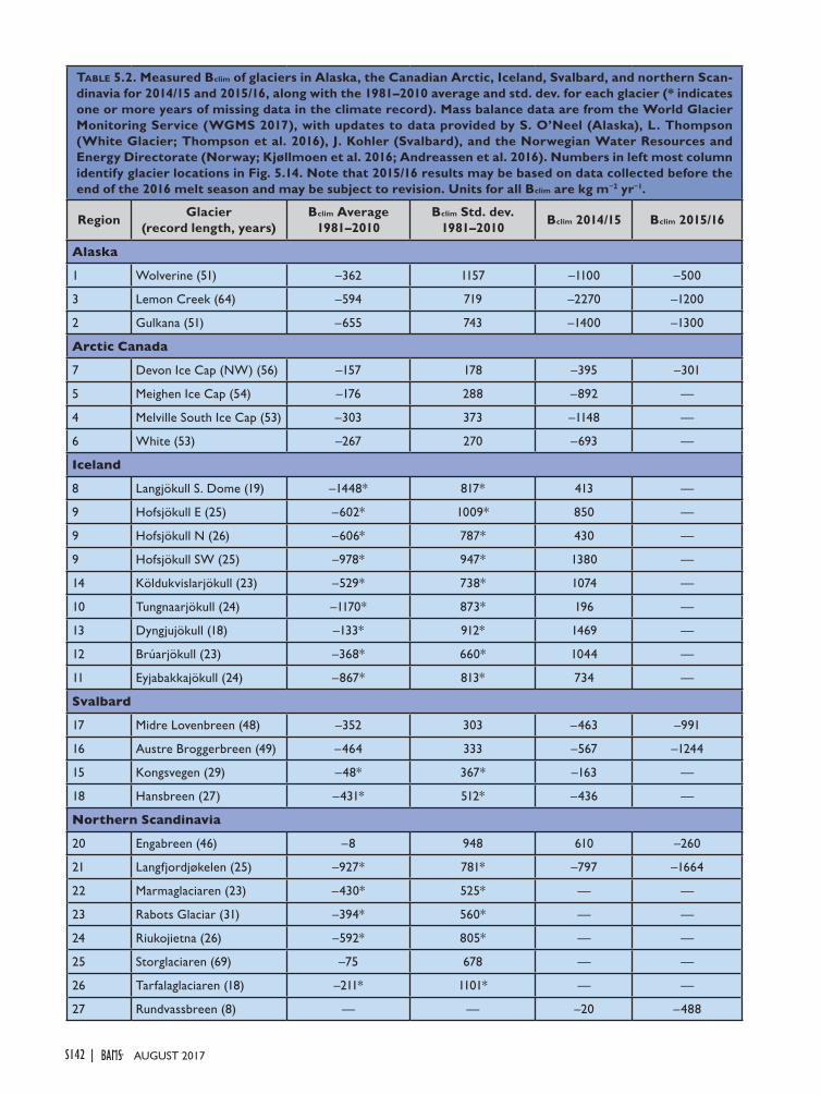
Table 5.2. Measured Bclim of glaciers in Alaska, the Canadian Arctic, Iceland, Svalbard, and northern Scan-dinavia for 2014/15 and 2015/16, along with the 1981–2010 average and std. dev. for each glacier (* indicates one or more years of missing data in the climate record). Mass balance data are from the World Glacier Monitoring Service (WGMS 2017), with updates to data provided by S. O’Neel (Alaska), L. Thompson (White Glacier; Thompson et al. 2016), J. Kohler (Svalbard), and the Norwegian Water Resources and Energy Directorate (Norway; Kjøllmoen et al. 2016; Andreassen et al. 2016). Numbers in left most column identify glacier locations in Fig. 5.14. Note that 2015/16 results may be based on data collected before the end of the 2016 melt season and may be subject to revision. Units for all Bclim are kg m−2 yr−1.

Region Glacier (record length, years)

Bclim Average 1981–2010

Bclim Std. dev. 1981–2010 Bclim 2014/15 Bclim 2015/16

Alaska

1 Wolverine (51) –362 1157 –1100 –500

3 Lemon Creek (64) –594 719 –2270 –1200

2 Gulkana (51) –655 743 –1400 –1300

Arctic Canada

7 Devon Ice Cap (NW) (56) –157 178 –395 –301

5 Meighen Ice Cap (54) –176 288 –892 —

4 Melville South Ice Cap (53) –303 373 –1148 —

6 White (53) –267 270 –693 —

Iceland

8 Langjökull S. Dome (19) –1448* 817* 413 —

9 Hofsjökull E (25) –602* 1009* 850 —

9 Hofsjökull N (26) –606* 787* 430 —

9 Hofsjökull SW (25) –978* 947* 1380 —

14 Köldukvislarjökull (23) –529* 738* 1074 —

10 Tungnaarjökull (24) –1170* 873* 196 —

13 Dyngjujökull (18) –133* 912* 1469 —

12 Brúarjökull (23) –368* 660* 1044 —

11 Eyjabakkajökull (24) –867* 813* 734 —

Svalbard

17 Midre Lovenbreen (48) –352 303 –463 –991

16 Austre Broggerbreen (49) –464 333 –567 –1244

15 Kongsvegen (29) –48* 367* –163 —

18 Hansbreen (27) –431* 512* –436 —

Northern Scandinavia

20 Engabreen (46) –8 948 610 –260

21 Langfjordjøkelen (25) –927* 781* –797 –1664

22 Marmaglaciaren (23) –430* 525* — —

23 Rabots Glaciar (31) –394* 560* — —

24 Riukojietna (26) –592* 805* — —

25 Storglaciaren (69) –75 678 — —

26 Tarfalaglaciaren (18) –211* 1101* — —

27 Rundvassbreen (8) — — –20 –488

AUGUST 2017|S142

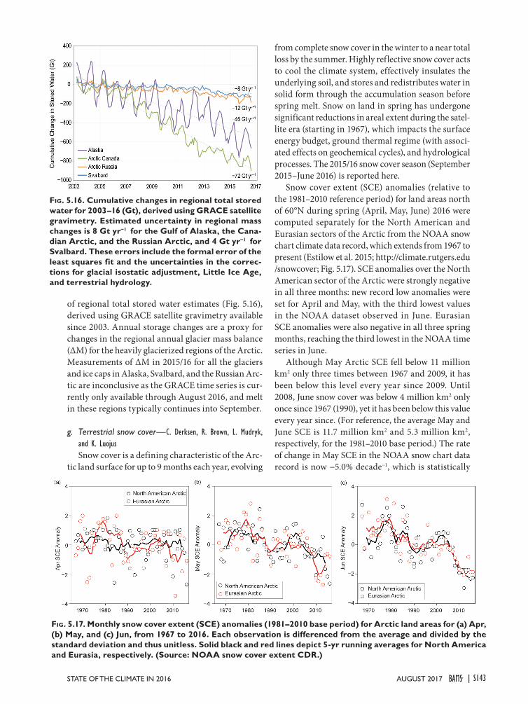
of regional total stored water estimates (Fig. 5.16), derived using GRACE satellite gravimetry available since 2003. Annual storage changes are a proxy for changes in the regional annual glacier mass balance (ΔM) for the heavily glacierized regions of the Arctic. Measurements of ΔM in 2015/16 for all the glaciers and ice caps in Alaska, Svalbard, and the Russian Arc-tic are inconclusive as the GRACE time series is cur-rently only available through August 2016, and melt in these regions typically continues into September.

g. Terrestrial snow cover—C. Derksen, R. Brown, L. Mudryk, and K. LuojusSnow cover is a defining characteristic of the Arc-

tic land surface for up to 9 months each year, evolving

from complete snow cover in the winter to a near total loss by the summer. Highly reflective snow cover acts to cool the climate system, effectively insulates the underlying soil, and stores and redistributes water in solid form through the accumulation season before spring melt. Snow on land in spring has undergone significant reductions in areal extent during the satel-lite era (starting in 1967), which impacts the surface energy budget, ground thermal regime (with associ-ated effects on geochemical cycles), and hydrological processes. The 2015/16 snow cover season (September 2015–June 2016) is reported here.

Snow cover extent (SCE) anomalies (relative to the 1981–2010 reference period) for land areas north of 60°N during spring (April, May, June) 2016 were computed separately for the North American and Eurasian sectors of the Arctic from the NOAA snow chart climate data record, which extends from 1967 to present (Estilow et al. 2015; http://climate.rutgers.edu /snowcover; Fig. 5.17). SCE anomalies over the North American sector of the Arctic were strongly negative in all three months: new record low anomalies were set for April and May, with the third lowest values in the NOAA dataset observed in June. Eurasian SCE anomalies were also negative in all three spring months, reaching the third lowest in the NOAA time series in June.

Although May Arctic SCE fell below 11 million km2 only three times between 1967 and 2009, it has been below this level every year since 2009. Until 2008, June snow cover was below 4 million km2 only once since 1967 (1990), yet it has been below this value every year since. (For reference, the average May and June SCE is 11.7 million km2 and 5.3 million km2, respectively, for the 1981–2010 base period.) The rate of change in May SCE in the NOAA snow chart data record is now −5.0% decade−1, which is statistically

Fig. 5.17. Monthly snow cover extent (SCE) anomalies (1981–2010 base period) for Arctic land areas for (a) Apr, (b) May, and (c) Jun, from 1967 to 2016. Each observation is differenced from the average and divided by the standard deviation and thus unitless. Solid black and red lines depict 5-yr running averages for North America and Eurasia, respectively. (Source: NOAA snow cover extent CDR.)

Fig. 5.16. Cumulative changes in regional total stored water for 2003–16 (Gt), derived using GRACE satellite gravimetry. Estimated uncertainty in regional mass changes is 8 Gt yr−1 for the Gulf of Alaska, the Cana-dian Arctic, and the Russian Arctic, and 4 Gt yr−1 for Svalbard. These errors include the formal error of the least squares fit and the uncertainties in the correc-tions for glacial isostatic adjustment, Little Ice Age, and terrestrial hydrology.


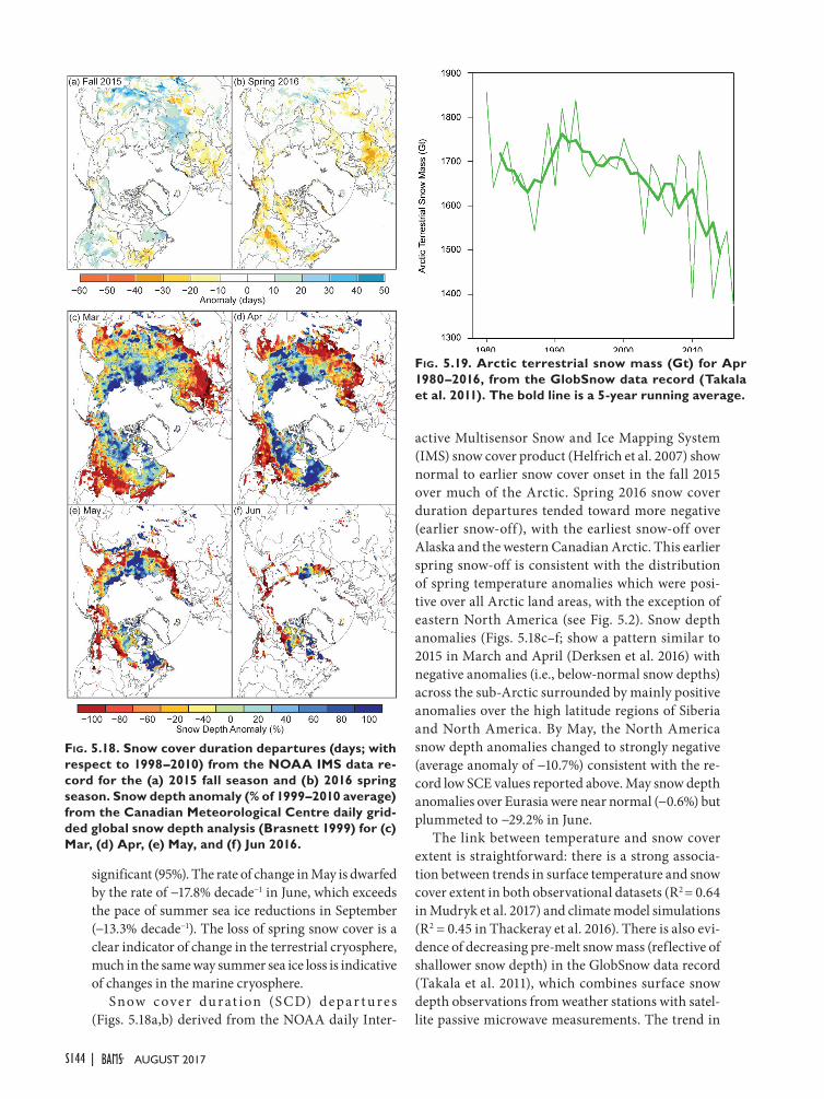
Fig. 5.18. Snow cover duration departures (days; with respect to 1998–2010) from the NOAA IMS data re-cord for the (a) 2015 fall season and (b) 2016 spring season. Snow depth anomaly (% of 1999–2010 average) from the Canadian Meteorological Centre daily grid-ded global snow depth analysis (Brasnett 1999) for (c) Mar, (d) Apr, (e) May, and (f) Jun 2016.

Fig. 5.19. Arctic terrestrial snow mass (Gt) for Apr 1980–2016, from the GlobSnow data record (Takala et al. 2011). The bold line is a 5-year running average.

significant (95%). The rate of change in May is dwarfed by the rate of −17.8% decade−1 in June, which exceeds the pace of summer sea ice reductions in September (−13.3% decade−1). The loss of spring snow cover is a clear indicator of change in the terrestrial cryosphere, much in the same way summer sea ice loss is indicative of changes in the marine cryosphere.

Snow cover du r at ion (SCD) depa r t u re s (Figs. 5.18a,b) derived from the NOAA daily Inter-

active Multisensor Snow and Ice Mapping System (IMS) snow cover product (Helfrich et al. 2007) show normal to earlier snow cover onset in the fall 2015 over much of the Arctic. Spring 2016 snow cover duration departures tended toward more negative (earlier snow-off), with the earliest snow-off over Alaska and the western Canadian Arctic. This earlier spring snow-off is consistent with the distribution of spring temperature anomalies which were posi-tive over all Arctic land areas, with the exception of eastern North America (see Fig. 5.2). Snow depth anomalies (Figs. 5.18c–f; show a pattern similar to 2015 in March and April (Derksen et al. 2016) with negative anomalies (i.e., below-normal snow depths) across the sub-Arctic surrounded by mainly positive anomalies over the high latitude regions of Siberia and North America. By May, the North America snow depth anomalies changed to strongly negative (average anomaly of −10.7%) consistent with the re-cord low SCE values reported above. May snow depth anomalies over Eurasia were near normal (−0.6%) but plummeted to −29.2% in June.

The link between temperature and snow cover extent is straightforward: there is a strong associa-tion between trends in surface temperature and snow cover extent in both observational datasets (R2 = 0.64 in Mudryk et al. 2017) and climate model simulations (R2 = 0.45 in Thackeray et al. 2016). There is also evi-dence of decreasing pre-melt snow mass (reflective of shallower snow depth) in the GlobSnow data record (Takala et al. 2011), which combines surface snow depth observations from weather stations with satel-lite passive microwave measurements. The trend in

AUGUST 2017|S144

April snow mass (the month of peak pre-melt Arctic snow mass) is −4.3% decade−1, with April 2016 hav-ing the lowest value in the record (Fig. 5.19). While early snow melt in previous years occurred despite above-average snow mass (e.g., 2011 and 2012), a shallower snowpack combined with above-average temperatures created ideal conditions for early and rapid snow melt, reflected in the new record low SCE values observed in 2016.

h. Tundra greenness—H. E. Epstein, U. S. Bhatt, M. K. Raynolds, D. A. Walker, B. C. Forbes, M. Macias-Fauria, M. Loranty, G. Phoenix, and J. BjerkeVegetation in the Arctic tundra has been respond-

ing dynamically to environmental changes, many of which are anthropogenically induced, since at least

the early 1980s. These vegetation changes throughout the circumpolar Arctic are not spatially homogenous, nor are they temporally consistent (e.g., Bhatt et al. 2013), suggesting that there are complex interactions among the atmosphere, ground (soils and perma-frost), vegetation, and herbivore components of the Arctic system. Changes in Arctic tundra vegetation may have a relatively small impact on the global carbon budget through photosynthetic uptake of CO2 compared to changes in other carbon cycling processes (Abbott et al. 2016). However, tundra veg-etation can have important effects on permafrost, hydrology, soil carbon fluxes, and the surface energy balance (e.g., Blok et el. 2010; Myers-Smith and Hik 2013; Parker et al. 2015). Tundra vegetation dynam-ics also control the diversity of herbivores (birds and

SIDEBAR 5.2: ARCTIC OCEAN ACIDIFICATION—J. N. CROSS AND J. T. MATHIS

A growing body of recent research has shown that the Arctic Ocean has rapidly acidified over the last several decades, in part due to the oceanic uptake of anthropo-genic carbon dioxide (CO2) from the atmosphere (e.g., Semiletov et al. 2016; Cross et al. 2017; Qi et al. 2017). While this long-term decrease in ocean pH does not produce acidic (e.g., pH <7) oceans, this gradual ocean acidification (OA) has been shown to compound natural variability in seawater carbonate chemistry. In some areas like the Arctic, the pH conditions observed today are now corrosive to biologically important carbonate minerals. Some studies indicate that these corrosive conditions can cover up to 40% of the Chukchi Sea benthos seasonally (Bates et al. 2013), and persist for 80% of the year in some hotspots (Cross et al. 2017).

Over the past five years, ocean acidif ication has emerged as one of the most prominent issues in marine research, especially given newfound public understand-ing of the potential biological threat to marine calcifiers (e.g., clams, pteropods) and associated fisheries, and the human impacts it poses for communities that directly or indirectly rely on them (e.g., Mathis et al. 2015a; Frisch et al. 2015). Cooler water and unique physical processes (i.e., formation and melting of sea ice) make the waters of the Arctic Ocean disproportionately sensitive to OA when compared to the rest of the global ocean. Even small amounts of human-derive (CO2) can cause significant chemical changes in the Arctic that other areas do not ex-perience; these could pose a threat to Arctic populations of calcifying marine organisms and their natural predators.

Recently, several comprehensive data synthesis prod-ucts (Bates 2015; Cross et al. 2017; Semiletov et al. 2016; Qi et al. 2017) were published using much of the available OA data collected in the Arctic Ocean. Several trends have emerged that clearly elucidate the rapid progres-sion of OA across the Arctic Basin, including rapid CO2 uptake from the atmosphere and increasing carbonate mineral corrosivity (e.g., Evans et al. 2015). A new analysis released this year suggests that corrosive conditions have been expanding since the late 1990s, spreading northward into the Arctic Basin over a thicker layer (Qi et al. 2017). These Pacific-origin corrosive waters have been observed as far north as the entrances to Amundsen Gulf and M’Clure Strait in the Canadian Arctic Archipelago (Cross et al. 2017).

Though the specifics remain uncertain, it is likely that the consequences of continuing OA will be detrimental for parts of the Arctic food web (Mathis et al. 2015a). For example, many large predators (e.g., seals, walrus, and salmon) rely on the small marine calcifiers most likely to be impacted by OA (Cross et al. 2017). Juvenile and larval life stages of some organisms are also particularly vulner-able to OA (e.g., crabs, Punt et al. 2014; shellfish, Ekstrom et al. 2015). In turn, many subsistence communities rely on seals, walrus, salmon, and other large predators. While biological impacts of OA are not presently visible, it is likely that OA conditions will intensify over the next two to three decades and may produce more prominent food web impacts with economic, ecological, and cultural implications (Mathis et al. 2015b; Punt et al. 2016).


mammals) in the Arctic, with species richness being positively related to vegetation productivity (Barrio et al. 2016).

Earth observing satellites with daily return in-tervals have provided the capacity to monitor Arctic tundra vegetation continuously since 1982. The data here are from the Global Inventory Modeling and Mapping Studies (GIMMS) version 3g dataset based largely on the AVHRR sensor onboard NOAA satel-

lites (Pinzon and Tucker 2014). The GIMMS product is a biweekly, maximum-value composited dataset of the normalized difference vegetation index (NDVI); NDVI is highly correlated with aboveground vegeta-tion (e.g., Raynolds et al. 2012). Two metrics based on the NDVI are used: MaxNDVI (peak NDVI for the yearly growing season, related to yearly maximum aboveground vegetation biomass) and time-inte-grated NDVI (TI-NDVI; sum of the biweekly NDVI values for the growing season, related to the total aboveground vegetation productivity). This section reports only through the end of the 2015 growing season (May–September), as a complete 2016 dataset was not available at the time of writing.

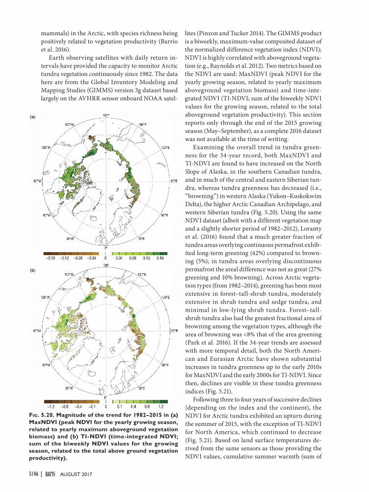
Examining the overall trend in tundra green-ness for the 34-year record, both MaxNDVI and TI-NDVI are found to have increased on the North Slope of Alaska, in the southern Canadian tundra, and in much of the central and eastern Siberian tun-dra, whereas tundra greenness has decreased (i.e., “browning”) in western Alaska (Yukon–Kuskokwim Delta), the higher Arctic Canadian Archipelago, and western Siberian tundra (Fig. 5.20). Using the same NDVI dataset (albeit with a different vegetation map and a slightly shorter period of 1982–2012), Loranty et al. (2016) found that a much greater fraction of tundra areas overlying continuous permafrost exhib-ited long-term greening (42%) compared to brown-ing (5%); in tundra areas overlying discontinuous permafrost the areal difference was not as great (27% greening and 10% browning). Across Arctic vegeta-tion types (from 1982–2014), greening has been most extensive in forest–tall-shrub tundra, moderately extensive in shrub tundra and sedge tundra, and minimal in low-lying shrub tundra. Forest–tall-shrub tundra also had the greatest fractional area of browning among the vegetation types, although the area of browning was <8% that of the area greening (Park et al. 2016). If the 34-year trends are assessed with more temporal detail, both the North Ameri-can and Eurasian Arctic have shown substantial increases in tundra greenness up to the early 2010s for MaxNDVI and the early 2000s for TI-NDVI. Since then, declines are visible in these tundra greenness indices (Fig. 5.21).

Following three to four years of successive declines (depending on the index and the continent), the NDVI for Arctic tundra exhibited an upturn during the summer of 2015, with the exception of TI-NDVI for North America, which continued to decrease (Fig. 5.21). Based on land surface temperatures de-rived from the same sensors as those providing the NDVI values, cumulative summer warmth (sum of

Fig. 5.20. Magnitude of the trend for 1982–2015 in (a) MaxNDVI (peak NDVI for the yearly growing season, related to yearly maximum aboveground vegetation biomass) and (b) TI-NDVI (time-integrated NDVI; sum of the biweekly NDVI values for the growing season, related to the total above ground vegetation productivity).

AUGUST 2017|S146

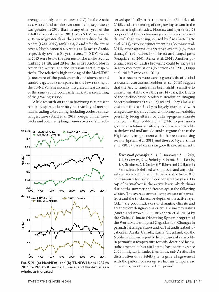
average monthly temperatures > 0°C) for the Arctic as a whole (and for the two continents separately) was greater in 2015 than in any other year of the satellite record (since 1982). MaxNDVI values in 2015 were greater than the average values for the record (1982–2015), ranking 8, 7, and 9 for the entire Arctic, North American Arctic, and Eurasian Arctic, respectively, over the 34-year record. TI-NDVI values in 2015 were below the average for the entire record, ranking 28, 28, and 29 for the entire Arctic, North American Arctic, and the Eurasian Arctic, respec-tively. The relatively high ranking of the MaxNDVI (a measure of the peak quantity of aboveground tundra vegetation) compared to the low ranking of the TI-NDVI (a seasonally integrated measurement of the same) could potentially indicate a shortening of the growing season.

While research on tundra browning is at present relatively sparse, there may be a variety of mecha-nisms leading to browning, including cooler summer temperatures (Bhatt et al. 2013), deeper winter snow packs and potentially longer snow cover duration ob-

served specifically in the tundra region (Bieniek et al. 2015), and a shortening of the growing season in the northern high latitudes. Phoenix and Bjerke (2016) propose that tundra browning could be more “event driven” than greening, caused by fire (Bret-Harte et al. 2013), extreme winter warming (Bokhorst et al. 2011), other anomalous weather events (e.g., frost damage), and outbreaks of insect and fungal pests (Graglia et al. 2001; Bjerke et al. 2014). Another po-tential cause of tundra browning could be increases in herbivore populations (Pederson et al. 2013; Hupp et al. 2015; Barrio et al. 2016).

In a recent remote sensing analysis of global terrestrial ecosystems, Seddon et al. (2016) suggest that the Arctic tundra has been highly sensitive to climate variability over the past 14 years, the length of the satellite-based Moderate Resolution Imaging Spectroradiometer (MODIS) record. They also sug-gest that this sensitivity is largely correlated with temperature and cloudiness, environmental variables presently being altered by anthropogenic climate change. Further, Seddon et al. (2016) report much greater vegetation sensitivity to climatic variability in the low and midlatitude tundra regions than in the High Arctic, in agreement with other remote sensing results (Epstein et al. 2012) and those of Myers-Smith et al. (2015), based on in situ growth measurements.

i. Terrestrial permafrost—V. E. Romanovsky, S. L. Smith,

N. I. Shiklomanov, D. A. Streletskiy, K. Isaksen, A. L. Kholodov, H. H. Christiansen, D. S. Drozdov, G. V. Malkova, and S. S. MarchenkoPermafrost is defined as soil, rock, and any other

subsurface earth material that exists at or below 0°C continuously for two or more consecutive years. On top of permafrost is the active layer, which thaws during the summer and freezes again the following winter. The average annual temperature of perma-frost and the thickness, or depth, of the active layer (ALT) are good indicators of changing climate and are therefore designated as essential climate variables (Smith and Brown 2009; Biskaborn et al. 2015) by the Global Climate Observing System program of the World Meteorological Organization. Changes in permafrost temperatures and ALT at undisturbed lo-cations in Alaska, Canada, Russia, Greenland, and the Nordic region are reported here. Regional variability in permafrost temperature records, described below, indicates more substantial permafrost warming since 2000 in higher latitudes than in the sub-Arctic. The distribution of variability is in general agreement with the pattern of average surface air temperature anomalies, over this same time period.

Fig. 5.21. (a) MaxNDVI and (b) TI-NDVI from 1982 to 2015 for North America, Eurasia, and the Arctic as a whole, as indicated.


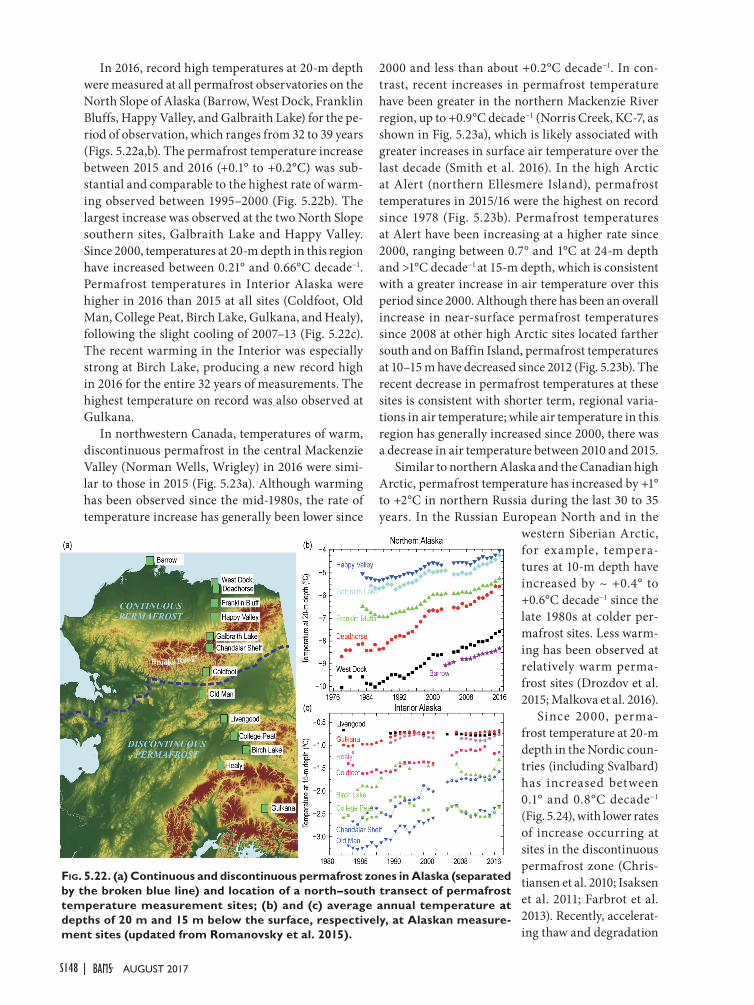
In 2016, record high temperatures at 20-m depth were measured at all permafrost observatories on the North Slope of Alaska (Barrow, West Dock, Franklin Bluffs, Happy Valley, and Galbraith Lake) for the pe-riod of observation, which ranges from 32 to 39 years (Figs. 5.22a,b). The permafrost temperature increase between 2015 and 2016 (+0.1° to +0.2°C) was sub-stantial and comparable to the highest rate of warm-ing observed between 1995–2000 (Fig. 5.22b). The largest increase was observed at the two North Slope southern sites, Galbraith Lake and Happy Valley. Since 2000, temperatures at 20-m depth in this region have increased between 0.21° and 0.66°C decade−1. Permafrost temperatures in Interior Alaska were higher in 2016 than 2015 at all sites (Coldfoot, Old Man, College Peat, Birch Lake, Gulkana, and Healy), following the slight cooling of 2007–13 (Fig. 5.22c). The recent warming in the Interior was especially strong at Birch Lake, producing a new record high in 2016 for the entire 32 years of measurements. The highest temperature on record was also observed at Gulkana.

In northwestern Canada, temperatures of warm, discontinuous permafrost in the central Mackenzie Valley (Norman Wells, Wrigley) in 2016 were simi-lar to those in 2015 (Fig. 5.23a). Although warming has been observed since the mid-1980s, the rate of temperature increase has generally been lower since

2000 and less than about +0.2°C decade−1. In con-trast, recent increases in permafrost temperature have been greater in the northern Mackenzie River region, up to +0.9°C decade−1 (Norris Creek, KC-7, as shown in Fig. 5.23a), which is likely associated with greater increases in surface air temperature over the last decade (Smith et al. 2016). In the high Arctic at Alert (northern Ellesmere Island), permafrost temperatures in 2015/16 were the highest on record since 1978 (Fig. 5.23b). Permafrost temperatures at Alert have been increasing at a higher rate since 2000, ranging between 0.7° and 1°C at 24-m depth and >1°C decade−1 at 15-m depth, which is consistent with a greater increase in air temperature over this period since 2000. Although there has been an overall increase in near-surface permafrost temperatures since 2008 at other high Arctic sites located farther south and on Baffin Island, permafrost temperatures at 10–15 m have decreased since 2012 (Fig. 5.23b). The recent decrease in permafrost temperatures at these sites is consistent with shorter term, regional varia-tions in air temperature; while air temperature in this region has generally increased since 2000, there was a decrease in air temperature between 2010 and 2015.

Similar to northern Alaska and the Canadian high Arctic, permafrost temperature has increased by +1° to +2°C in northern Russia during the last 30 to 35 years. In the Russian European North and in the

western Siberian Arctic, for example, tempera-tures at 10-m depth have increased by ~ +0.4° to +0.6°C decade−1 since the late 1980s at colder per-mafrost sites. Less warm-ing has been observed at relatively warm perma-frost sites (Drozdov et al. 2015; Malkova et al. 2016).

Since 2000, perma-frost temperature at 20-m depth in the Nordic coun-tries (including Svalbard) has increased between 0.1° and 0.8°C decade−1 (Fig. 5.24), with lower rates of increase occurring at sites in the discontinuous permafrost zone (Chris-tiansen et al. 2010; Isaksen et al. 2011; Farbrot et al. 2013). Recently, accelerat-ing thaw and degradation

Fig. 5.22. (a) Continuous and discontinuous permafrost zones in Alaska (separated by the broken blue line) and location of a north–south transect of permafrost temperature measurement sites; (b) and (c) average annual temperature at depths of 20 m and 15 m below the surface, respectively, at Alaskan measure-ment sites (updated from Romanovsky et al. 2015).

AUGUST 2017|S148

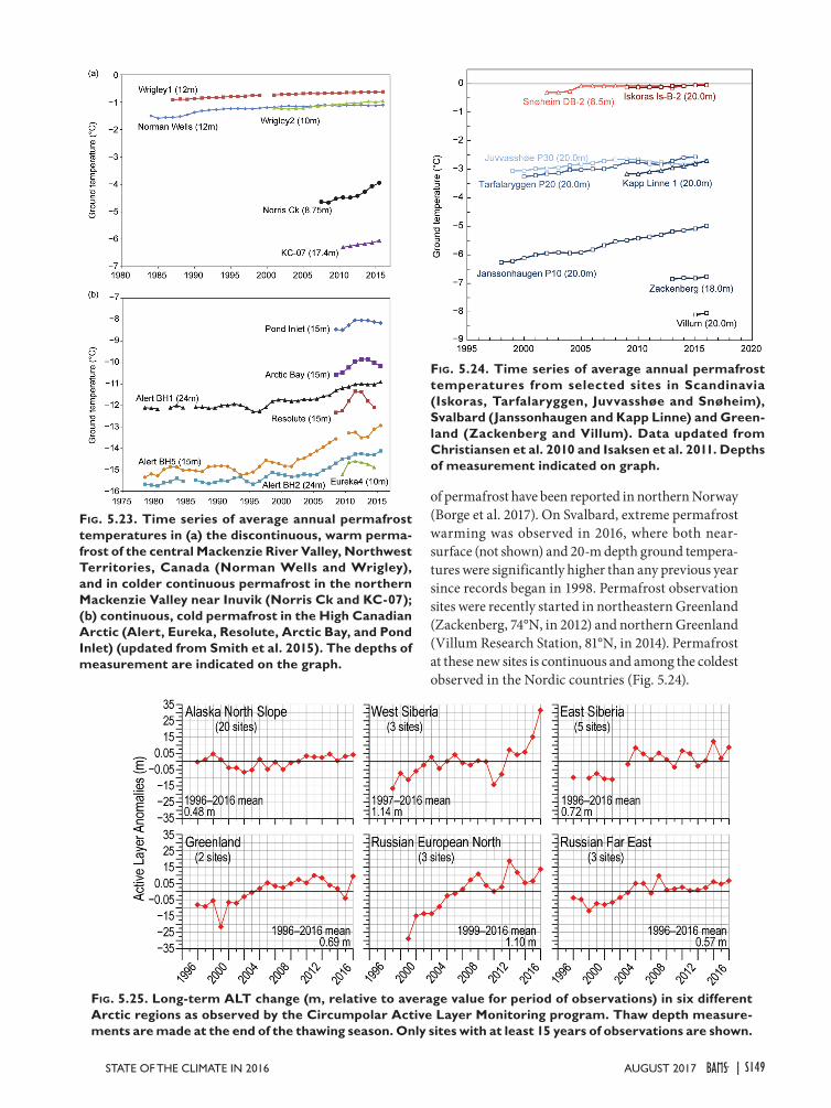
Fig. 5.23. Time series of average annual permafrost temperatures in (a) the discontinuous, warm perma-frost of the central Mackenzie River Valley, Northwest Territories, Canada (Norman Wells and Wrigley), and in colder continuous permafrost in the northern Mackenzie Valley near Inuvik (Norris Ck and KC-07); (b) continuous, cold permafrost in the High Canadian Arctic (Alert, Eureka, Resolute, Arctic Bay, and Pond Inlet) (updated from Smith et al. 2015). The depths of measurement are indicated on the graph.

Fig. 5.24. Time series of average annual permafrost temperatures from selected sites in Scandinavia (Iskoras, Tarfalaryggen, Juvvasshøe and Snøheim), Svalbard (Janssonhaugen and Kapp Linne) and Green-land (Zackenberg and Villum). Data updated from Christiansen et al. 2010 and Isaksen et al. 2011. Depths of measurement indicated on graph.

of permafrost have been reported in northern Norway (Borge et al. 2017). On Svalbard, extreme permafrost warming was observed in 2016, where both near-surface (not shown) and 20-m depth ground tempera-tures were significantly higher than any previous year since records began in 1998. Permafrost observation sites were recently started in northeastern Greenland (Zackenberg, 74°N, in 2012) and northern Greenland (Villum Research Station, 81°N, in 2014). Permafrost at these new sites is continuous and among the coldest observed in the Nordic countries (Fig. 5.24).

Fig. 5.25. Long-term ALT change (m, relative to average value for period of observations) in six different Arctic regions as observed by the Circumpolar Active Layer Monitoring program. Thaw depth measure-ments are made at the end of the thawing season. Only sites with at least 15 years of observations are shown.


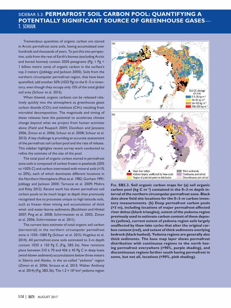
SIDEBAR 5.3: PERMAFROST SOIL CARBON POOL: QUANTIFYING A POTENTIALLY SIGNIFICANT SOURCE OF GREENHOUSE GASES—T. SCHUUR

Tremendous quantities of organic carbon are stored in Arctic permafrost zone soils, having accumulated over hundreds and thousands of years. To put this into perspec-tive, soils from the rest of Earth’s biomes (excluding Arctic and boreal biomes) contain 2050 petagrams (Pg; 1 Pg = 1 billion metric tons) of organic carbon in the surface’s top 3 meters (Jobbágy and Jackson 2000). Soils from the northern circumpolar permafrost region, that have been quantified, add another 50% (1025 Pg) to the 0–3 m inven-tory, even though they occupy only 15% of the total global soil area (Schuur et al. 2015).

When thawed, organic carbons can be released rela-tively quickly into the atmosphere as greenhouse gases carbon dioxide (CO2) and methane (CH4) resulting from microbial decomposition. The magnitude and timing of these releases have the potential to accelerate climate change beyond what we project from human activities alone (Field and Raupach 2004; Davidson and Janssens 2006; Zimov et al. 2006; Schuur et al. 2008; Schuur et al. 2013). A key challenge is providing an accurate assessment of the permafrost soil carbon pool and the rate of release. This sidebar highlights recent survey work conducted to refine the estimate of the size of the pool.

The total pool of organic carbon stored in permafrost zone soils is composed of carbon frozen in peatlands (20% to >50% C) and carbon intermixed with mineral soils (<1% to 20%), each of which dominates different locations in the Northern Hemisphere (Post et al. 1982; Gorham 1991; Jobbagy and Jackson 2000; Tarnocai et al. 2009; Mishra and Riley 2012). Recent work has shown permafrost soil carbon pools to be much larger at depth than previously recognized due to processes unique to high latitude soils, such as freeze–thaw mixing and accumulation of thick wind- and water-borne sediments (Bockheim and Hinkel 2007; Ping et al. 2008; Schirrmeister et al. 2002; Zimov et al. 2006; Schirrmeister et al. 2011).

The current best estimate of total organic soil carbon (terrestrial) in the northern circumpolar permafrost zone is 1330–1580 Pg (Schuur et al. 2015; Hugelius et al. 2014). All permafrost-zone soils estimated to 3-m depth contain 1035 ± 150 Pg C (Fig. SB5.3a). New revisions place between 210 ± 70 and 456 ± 45 Pg C in deep loess (wind-blown sediment) accumulations below three meters in Siberia and Alaska, in the so-called “yedoma” region (Zimov et al. 2006; Strauss et al. 2013; Walter Anthony et al. 2014) (Fig. SB5.3b). The 1.2 × 106 km2 yedoma region

Fig. SB5.3. Soil organic carbon maps for (a) soil organic carbon pool (kg C m−2) contained in the 0–3-m depth in-terval of the northern circumpolar permafrost zone. Black dots show field site locations for the 0–3-m carbon inven-tory measurements. (b) Deep permafrost carbon pools (>3 m), including locations of major permafrost-affected river deltas (black triangles), extent of the yedoma region previously used to estimate carbon content of these depos-its (yellow), current extent of yedoma region soils largely unaffected by thaw-lake cycles that alter the original car-bon content (red), and extent of thick sediments overlying bedrock (black hashed). Yedoma regions are generally also thick sediments. The base map layer shows permafrost distribution with continuous regions to the north hav-ing permafrost everywhere (>90%, purple shading), and discontinuous regions farther south having permafrost in some, but not all, locations (<90%, pink shading).

AUGUST 2017|S150

remained ice free during the last Ice Age. Even though carbon concentrations of these mineral soils are not remarkably high (0.2%–2% C) the depths of these sedi-ments give rise to large carbon inventories. Additional deep carbon pools beyond yedoma include river deltas, which are now thought to contain 91 ± 39 Pg C, much less than was originally estimated for these deep deposits (Hugelius et al 2014; Tarnocai et al. 2009).

Three additional pools of permafrost carbon not yet included in the permafrost carbon pool summarized here are: (1) the permafrost region of the Tibetan plateau and permafrost soils in northern China; (2) other deep terrestrial sediment deposits located over 5 × 106 km2 outside the yedoma and delta areas; and (3) a reservoir of organic carbon stored in permafrost on the continental shelf under the Arctic Ocean (Rogers and Morack 1980; Brown et al. 1998, revised February 2001). The amount of organic carbon in the Tibetan and North China region is currently estimated at 35.7 Pg (Luo et al. 2000; Wang et al. 2008; Mu et al. 2015; Ding et al. 2016). Simple cal-culations based on extremely limited data suggest that another ~350–465 Pg C can be found in additional deep terrestrial deposits, although more sampling and data syn-

thesis need to be done to verify or revise these potential deep permafrost carbon deposits (Schuur et al. 2015).

There are no reliable published estimates of total organic carbon inventory for the subsea permafrost pool. Undersea permafrost carbon initially formed on land as the continental shelf was exposed by sea levels that were 120 meters lower during the last glacial period (Walter et al. 2007). Subsequent inundation of this area at the Pleis-tocene/Holocene transition put this loess permafrost car-bon under water and also started thawing the permafrost surface (Rachold et al. 2007). Much of the shallow shelf is thought to have been covered with yedoma deposits when it was exposed during the last glacial period. The shallow shelf area exposed as dry land in the area around Alaska and Siberia during the last Ice Age is about 2.5 times the size of the current terrestrial yedoma region (Strauss et al. 2013; Brosius et al. 2012). Submergence over thousands of years helped to thaw the permafrost, exposing organic carbon to decomposition potentially under anaerobic conditions. This would have converted a portion of the carbon pool to CO2 and CH4 in the past, leaving an un-known quantity of organic carbon remaining both in the sediment and in permafrost that persists under the ocean.

In 2016, the active layer thickness (determined by mechanical probing) at all Arctic sites was at or near the long-term maximum for the entire period of observation, which ranges from 18 to 21 years (Fig. 5.25). The all-period record high was observed in 2016 at the West Siberian sites. At the Alaska North Slope and Greenland sites, ALT reached the previ-ously observed maxima, achieved in 1998 and 2013 (North Slope) and 2011 (Greenland). At the rest of the sites the 2016 values were the second highest for the entire period of observation. The largest increase in ALT (0.31 m) during the last two years was observed at the West Siberia sites, where ALT reached an ab-solute maximum of 1.45 m over the 20-year period of observation, suggesting that at some locations the active layer may not be freezing back completely during the winter.

j. Ozone and UV radiation—G. H. Bernhard, V. E. Fioletov, J.-U. Grooß, I. Ialongo, B. Johnsen, K. Lakkala, G. L. Manney, and R. Müller This report emphasizes the period November 2015

to April 2016 because chemically-induced loss of polar ozone mostly occurs during winter and spring (WMO 2014). These chemical processes are initiated by low temperatures in the lower stratosphere (alti-tude of approximately 15 to 25 km) in the presence of chlorine-containing substances (e.g., HCl and ClONO2). Temperatures in the Arctic stratosphere during November and December 2015 were the lowest in the 68-year observational record (Matthias et al. 2016), and temperatures in January 2016 were the lowest since at least 1979 (Manney and Lawrence 2016). Between 16 November 2015 and 10 March 2016, temperatures below about 195 K (−78°C) led to the formation of polar stratospheric clouds (PSCs), which act as a catalyst to transform inactive forms of chlorine to active, ozone-destroying substances.


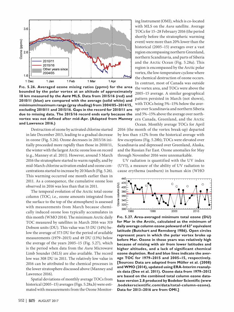
ing Instrument (OMI), which is co-located with MLS on the Aura satellite. Average TOCs for 15–28 February 2016 (the period shortly before the stratospheric warming event) were more than 20% lower than the historical (2005–15) averages over a vast region encompassing northern Greenland, northern Scandinavia, and parts of Siberia and the Arctic Ocean (Fig. 5.28a). This region is encompassed by the Arctic polar vortex, the low-temperature cyclone where the chemical destruction of ozone occurs. In contrast, most of Canada was outside the vortex area, and TOCs were above the 2005–15 average. A similar geographical pattern persisted in March (not shown), with TOCs being 5%–15% below the aver-age over Scandinavia and northern Siberia and 5%–15% above the average over north-ern Canada, Greenland, and the Arctic Ocean. Monthly average TOCs for April

2016 (the month of the vortex break-up) departed by less than ±12% from the historical average with few exceptions (Fig. 5.28b); TOCs were elevated over Scandinavia and depressed over Greenland, Alaska, and the Russian Far East. Ozone anomalies for May through November 2016 were unremarkable.

UV radiation is quantified with the UV index (UVI), a measure of the ability of UV radiation to cause erythema (sunburn) in human skin (WHO

Destruction of ozone by activated chlorine started in late December 2015, leading to a gradual decrease in ozone (Fig. 5.26). Ozone decreases in 2015/16 ini-tially proceeded more rapidly than those in 2010/11, the winter with the largest Arctic ozone loss on record (e.g., Manney et al. 2011). However, around 5 March 2016 the stratosphere started to warm rapidly, and by mid-March chlorine activation ended and ozone con-centrations started to increase by 20 March (Fig. 5.26). This warming occurred one month earlier than in 2011. As a consequence, the cumulative ozone loss observed in 2016 was less than that in 2011.

The temporal evolution of the Arctic total ozone column (TOC; i.e., ozone amounts integrated from the surface to the top of the atmosphere) is assessed with measurements from March because chemi-cally induced ozone loss typically accumulates in this month (WMO 2014). The minimum Arctic daily TOC measured by satellites in March 2016 was 319 Dobson units (DU). This value was 53 DU (14%) be-low the average of 373 DU for the period of available measurements (1979–2015) and 49 DU (13%) below the average of the years 2005–15 (Fig. 5.27), which is the period when data from the Aura Microwave Limb Sounder (MLS) are also available. The record low was 308 DU in 2011. The relatively low value in 2016 can be attributed to the chemical processes in the lower stratosphere discussed above (Manney and Lawrence 2016).

Spatial deviations of monthly average TOCs from historical (2005–15) averages (Figs. 5.28a,b) were esti-mated with measurements from the Ozone Monitor-

Fig. 5.26. Averaged ozone mixing ratios (ppmv) for the area bounded by the polar vortex at an altitude of approximately 18 km measured by the Aura MLS. Data from 2015/16 (red) and 2010/11 (blue) are compared with the average (solid white) and minimum/maximum range (gray shading) from 2004/05–2014/15, excluding 2010/11 and 2015/16. Gaps in the record for 2010/11 are due to missing data. The 2015/16 record ends early because the vortex was not defined after mid-Apr. (Adapted from Manney and Lawrence 2016.)

Fig. 5.27. Area-averaged minimum total ozone (DU) for Mar in the Arctic, calculated as the minimum of daily average column ozone poleward of 63° equivalent latitude (Butchart and Remsberg 1986). Open circles represent years in which the polar vortex broke up before Mar. Ozone in those years was relatively high because of mixing with air from lower latitudes and higher altitudes, and a lack of significant chemical ozone depletion. Red and blue lines indicate the aver-age TOC for 1979–2015 and 2005–15, respectively. [Sources: Data are adapted from Müller et al. (2008) and WMO (2014), updated using ERA-Interim reanaly-sis data (Dee et al. 2011). Ozone data from 1979–2012 are based on the combined total column ozone data-base version 2.8 produced by Bodeker Scientific (www .bodekerscientific.com/data/total-column-ozone). Data for 2013–2016 are from OMI.]

AUGUST 2017|S152

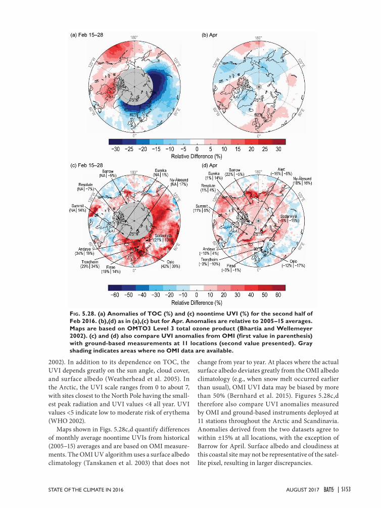
2002). In addition to its dependence on TOC, the UVI depends greatly on the sun angle, cloud cover, and surface albedo (Weatherhead et al. 2005). In the Arctic, the UVI scale ranges from 0 to about 7, with sites closest to the North Pole having the small-est peak radiation and UVI values <4 all year. UVI values <5 indicate low to moderate risk of erythema (WHO 2002).

Maps shown in Figs. 5.28c,d quantify differences of monthly average noontime UVIs from historical (2005–15) averages and are based on OMI measure-ments. The OMI UV algorithm uses a surface albedo climatology (Tanskanen et al. 2003) that does not

change from year to year. At places where the actual surface albedo deviates greatly from the OMI albedo climatology (e.g., when snow melt occurred earlier than usual), OMI UVI data may be biased by more than 50% (Bernhard et al. 2015). Figures 5.28c,d therefore also compare UVI anomalies measured by OMI and ground-based instruments deployed at 11 stations throughout the Arctic and Scandinavia. Anomalies derived from the two datasets agree to within ±15% at all locations, with the exception of Barrow for April. Surface albedo and cloudiness at this coastal site may not be representative of the satel-lite pixel, resulting in larger discrepancies.

Fig. 5.28. (a) Anomalies of TOC (%) and (c) noontime UVI (%) for the second half of Feb 2016. (b),(d) as in (a),(c) but for Apr. Anomalies are relative to 2005–15 averages. Maps are based on OMTO3 Level 3 total ozone product (Bhartia and Wellemeyer 2002). (c) and (d) also compare UVI anomalies from OMI (first value in parenthesis) with ground-based measurements at 11 locations (second value presented). Gray shading indicates areas where no OMI data are available.


Average noontime UVIs for 15–28 February 2016 (Fig. 5.28c) exceeded the 2005–15 averages by up to 60% over an area roughly matching the region where TOCs were abnormally low in 2016 (Fig. 5.28a). UVI anomalies show a larger spatial variability than TOCs because of their added dependence on cloud cover. While relative increases in the UVI were high, absolute increases remained below 1 UVI unit because solar elevations in February are below 23° for latitudes higher than 60°N (the latitude of Oslo,

Norway). Anomalies for March 2016 differed by less than ±15% from the historical average (not shown). Monthly average noontime UVIs for April 2016 were 5%–15% above the 2005–15 averages over most of the Arctic (Fig. 5.27d) with larger anomalies at Svalbard and the Denmark Strait east of Greenland. UVIs in southern Scandinavia were depressed in April. From May through November, UVIs at the ground stations varied within historical bounds.

AUGUST 2017|S154

5. the arctic - American Meteorological Society

Documents