5 Multiple regression analysis with qualitative information Multiple regression analysis with... · 5 Multiple regression analysis with qualitative information Ezequiel Uriel University

1

5 Multiple regression analysis with qualitative information Ezequiel Uriel University of Valencia Version: 09-2013

5.1 Introduction of qualitative information in econometric models. 1 5.2 A single dummy independent variable 2 5.3 Multiple categories for an attribute 5 5.4 Several attributes 8 5.5 Interactions involving dummy variables. 10

5.5.1 Interactions between two dummy variables 10 5.5.2 Interactions between a dummy variable and a quantitative variable 11

5.6 Testing structural changes 12 5.6.1 Using dummy variables 12 5.6.2 Using separate regressions: The Chow test 15

Exercises 18

5.1 Introducing qualitative information in econometric models.

Up until now, the variables that we have used in explaining the endogenous variable have a quantitative nature. However, there are other variables of a qualitative nature that can be important when explaining the behavior of the endogenous variable, such as sex, race, religion, nationality, geographical region etc. For example, holding all other factors constant, female workers are found to earn less than their male counterparts. This pattern may result from gender discrimination, but whatever the reason, qualitative variables such as gender seem to influence the regressand and clearly should be included in many cases among the explanatory variables, or the regressors. Qualitative factors often (although not always) come in the form of binary information, i.e. a person is male or female, is either married or not, etc. When qualitative factors come in the form of dichotomous information, the relevant information can be captured by defining a binary variable or a zero-one variable. In econometrics, binary variables used as regressors are commonly called dummy variables. In defining a dummy variable, we must decide which event is assigned the value one and which is assigned the value zero.

In the case of gender, we can define

1 if the person is a female

0 if the person is a malefemale

But of course we can also define

1 if the person is a male

0 if the person is a femalemale

Nevertheless, it is important to remark that both variables, male and female, contain the same information. Using zero-one variables for capturing qualitative information is an arbitrary decision, but with this election the parameters have a natural interpretation.

5.2 A single dummy independent variable

Let us see how we incorporate dichotomous information into regression models. Consider the simple model of hourly wage determination as a function of the years of education (educ):

2

1 2wage educ u (5-1)

To measure gender wage discrimination, we introduce a dummy variable for gender as an independent variable in the model defined above,

1 1 2wage female educ u (5-2)

The attribute gender has two categories: male and female. The female category has been included in the model, while the male category, which was omitted, is the reference category. Model 1 is shown in Figure 5.1, taking <0. The interpretation of is the following: is the difference in hourly wage between females and males, given the same amount of education (and the same error disturbance u). Thus, the coefficient determines whether there is discrimination against women or not. If <0 then, for the same level of other factors (education, in this case), women earn less than men on average. Assuming that the disturbance mean is zero, if we take expectation for both categories we obtain:

| 1 1 2

| 1 2

( | 1, )

( | 0, )

wage female

wage male

E wage female educ educ

E wage female educ educ

(5-3)

As can be seen in (5-3), the intercept is for males, and +for females. Graphically, as can be seen in Figure 5.1, there is a shift of the intercept, but the lines for men and women are parallel.

FIGURE 5.1. Same slope, different intercept.

In (5-2) we have included a dummy variable for female but not for male, because if we had included both dummies this would have been redundant. In fact, all we need is two intercepts, one for females and another one for males. As we have seen, if we introduce the female dummy variable, we have an intercept for each gender. Introducing two dummy variables would cause perfect multicollinearity given that female+male=1, which means that male is an exact linear function of female and of the intercept. Including dummy variables for both genders plus the intercept is the simplest example of the so-called dummy variable trap, as we shall show later on.

If we use male instead of female, the wage equation would be the following:

1 1 2wage male educ u (5-4)

wag

e

educ0

1

1

1 +

β2

β2

3

Nothing has changed with the new equation, except the interpretation of and : is the intercept for women, which is now the reference category, and +is the intercept for men. This implies the following relationship between the coefficients:

=+ and += =

In any application, it does not matter how we choose the reference category, since this only affects the interpretation of the coefficients associated to the dummy variables, but it is important to keep track of which category is the reference category. Choosing a reference category is usually a matter of convenience. It would also be possible to drop the intercept and to include a dummy variable for each category. The equation would then be

1 1 2wage male female educ u (5-5)

where the intercept is 1 for men and 1 for women.

Hypothesis testing is performed as usual. In model (5-2), the null hypothesis of no difference between men and women is 0 1: 0H , while the alternative hypothesis

that there is discrimination against women is 1 1: 0H . Therefore, in this case, we

must apply a one sided (left) t test.

A common specification in applied work has the dependent variable as the logarithm transformation ln(y) in models of this type. For example:

1 1 2ln( )wage female educ u (5-6)

Let us see the interpretation of the coefficient of the dummy variable in a log model. In model (5-6), taking u=0, the wage for a female and for a male is as follows:

1 1 2ln( )Fwage educ (5-7)

1 2ln( )Mwage educ (5-8)

Given the same amount of education, if we subtract (5-7) from (5-8), we have

1ln( ) ln( )F Mwage wage (5-9)

Taking antilogs in (5-9) and subtracting 1 from both sides of (5-9), we get

11 1F

M

wagee

wage (5-10)

That is to say

1 1F M

M

wage wagee

wage

(5-11)

According to (5-11), the proportional change between the female wage and the male wage, for the same amount of education, is equal to 1 1e . Therefore, the exact percentage change in hourly wage between men and women is 100 1( 1)e . As an

approximation to this change, 100×1 can be used. However, if the magnitude of the percentage is high, then this approximation is not so accurate.

EXAMPLE 5.1 Is there wage discrimination against women in Spain?

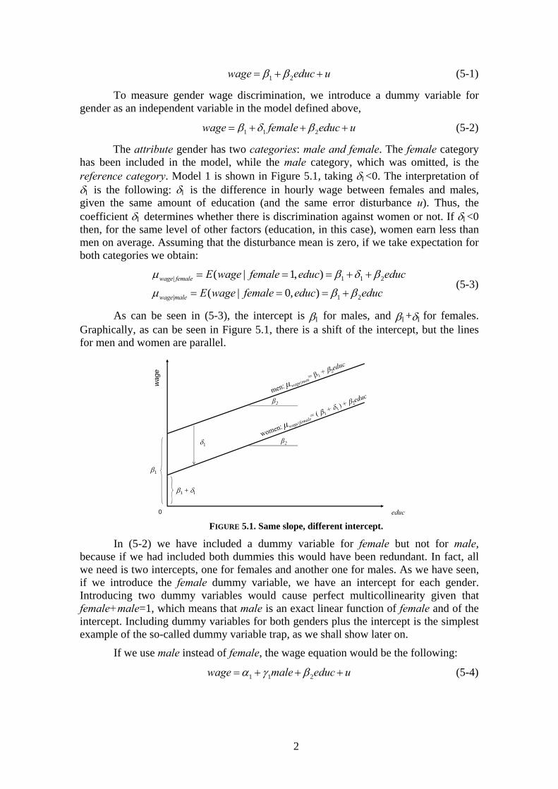
Using data from the wage structure survey of Spain for 2002 (file wage02sp), model (5-6) has been estimated and the following results were obtained:

4

(0.026) (0.022) (0.0025)

ln( ) 1.731 0.307 0.0548wage female educ = - +

RSS=393 R2=0.243 n=2000

where wage is hourly wage in euros, female is a dummy variable that takes the value 1 if it is a woman, and educ are the years of education. (The numbers in parentheses are standard errors of the estimators.)

To answer the question posed above, we need to test 0 1: 0H against 1 1: 0H . Given that

the t statistic is equal to -14.27, we reject the null hypothesis for =0.01. That is to say, there is a negative discrimination in Spain against women in the year 2002. In fact, the percentage difference in hourly wage between men and women is 0.307100 ( 1) 35.9%e , given the same years of education.

EXAMPLE 5.2 Analysis of the relation between market capitalization and book value: the role of ibex35

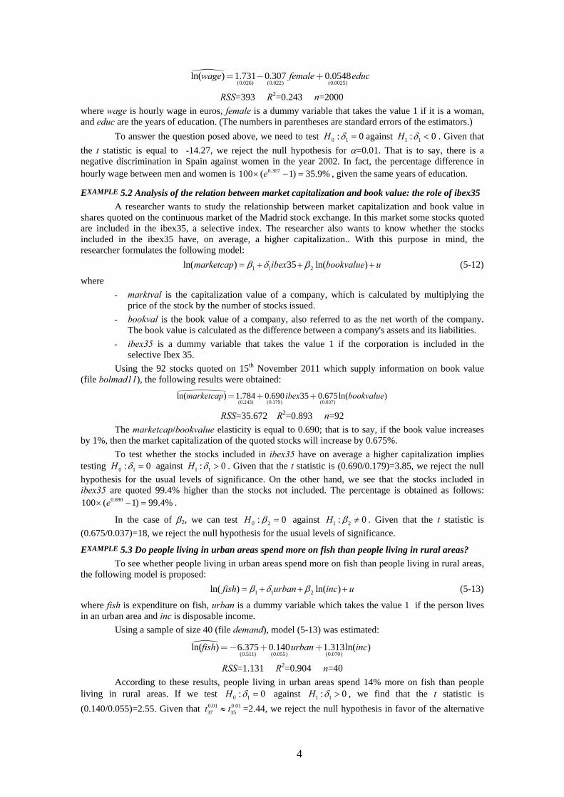
A researcher wants to study the relationship between market capitalization and book value in shares quoted on the continuous market of the Madrid stock exchange. In this market some stocks quoted are included in the ibex35, a selective index. The researcher also wants to know whether the stocks included in the ibex35 have, on average, a higher capitalization.. With this purpose in mind, the researcher formulates the following model:

1 1 2ln( ) 35 ln( )marketcap ibex bookvalue u (5-12)

where

- marktval is the capitalization value of a company, which is calculated by multiplying the price of the stock by the number of stocks issued.

- bookval is the book value of a company, also referred to as the net worth of the company. The book value is calculated as the difference between a company's assets and its liabilities.

- ibex35 is a dummy variable that takes the value 1 if the corporation is included in the selective Ibex 35.

Using the 92 stocks quoted on 15th November 2011 which supply information on book value (file bolmad11), the following results were obtained:

(0.243) (0.179) (0.037)

ln( ) 1.784 0.690 35 0.675ln( )marketcap ibex bookvalue= + +

RSS=35.672 R2=0.893 n=92

The marketcap/bookvalue elasticity is equal to 0.690; that is to say, if the book value increases by 1%, then the market capitalization of the quoted stocks will increase by 0.675%.

To test whether the stocks included in ibex35 have on average a higher capitalization implies testing 0 1: 0H against 1 1: 0H . Given that the t statistic is (0.690/0.179)=3.85, we reject the null

hypothesis for the usual levels of significance. On the other hand, we see that the stocks included in ibex35 are quoted 99.4% higher than the stocks not included. The percentage is obtained as follows:

0.690100 ( 1) 99.4%e .

In the case of 2, we can test 0 2: 0H against 1 2: 0H . Given that the t statistic is

(0.675/0.037)=18, we reject the null hypothesis for the usual levels of significance.

EXAMPLE 5.3 Do people living in urban areas spend more on fish than people living in rural areas?

To see whether people living in urban areas spend more on fish than people living in rural areas, the following model is proposed:

1 1 2ln( ) ln( )fish urban inc u (5-13)

where fish is expenditure on fish, urban is a dummy variable which takes the value 1 if the person lives in an urban area and inc is disposable income.

Using a sample of size 40 (file demand), model (5-13) was estimated:

(0.511) (0.055) (0.070)

ln( ) 6.375 0.140 1.313ln( )fish urban inc =- + +

RSS=1.131 R2=0.904 n=40

According to these results, people living in urban areas spend 14% more on fish than people living in rural areas. If we test 0 1: 0H against 1 1: 0H , we find that the t statistic is

(0.140/0.055)=2.55. Given that 0.01 0.0137 35t t =2.44, we reject the null hypothesis in favor of the alternative

5

for the usual levels of significance. That is to say, there is empirical evidence that people living in urban areas spend more on fish than people living in rural areas.

5.3 Multiple categories for an attribute

In the previous section we have seen an attribute (gender) that has two categories (male and female). Now we are going to consider attributes with more than two categories. In particular, we will examine an attribute with three categories

To measure the impact of firm size on wage, we can use a dummy variable. Let us suppose that firms are classified in three groups according to their size: small (up to 49 workers), medium (from 50 to 199 workers) and large (more than 199 workers). With this information, we can construct three dummy variables:

1 up to 49 workers

0 in other case

1 from 50 to 199 workers

0 in other case

1 more than 199 workers

0 in other case

small

medium

large

If we want to explain hourly wages by introducing the firm size in the model, we must omit one of the categories. In the following model, the omitted category is small firms:

1 1 2 2wage medium large educ u (5-14)

The interpretation of the j coefficients is the following: 1 (2) is the difference in hourly wage between medium (large) firms and small firms, given the same amount of education (and the same error term u).

Let us see what happens if we also include the category small in (5-14). We would have the model:

1 0 1 2 2wage small medium large educ u (5-15)

Now, let us consider that we have a sample of six observations: the observations 1 and 2 correspond to small firms; 3 and 4 to medium ones; and 5 and 6 to large ones. In this case the matrix of regressors X would have the following configuration:

1

2

3

4

5

6

1 1 0 0

1 1 0 0

1 0 1 0

1 0 1 0

1 0 0 1

1 0 0 1

educ

educ

educ

educ

educ

educ

X

As can be seen in matrix X, column 1 of this matrix is equal to the sum of columns 2, 3 and 4. Therefore, there is perfect multicollinearity due to the so-called dummy variable trap. Generalizing, if an attribute has g categories, we need to include only g1 dummy variables in the model along with the intercept. The intercept for the reference category is the overall intercept in the model, and the dummy variable

6

coefficient for a particular group represents the estimated difference in intercepts between that category and the reference category. If we include g dummy variables along with an intercept, we will fall into the dummy variable trap. An alternative is to include g dummy variables and to exclude an overall intercept. In the case we are examining, the model would be the following:

0 1 2 2wage small medium large educ u (5-16)

This solution is not advisable for two reasons. With this configuration of the model it is more difficult to test differences with respect to a reference category. Second, this solution only works in the case of a model with only one unique attribute.

EXAMPLE 5.4 Does firm size influence wage determination?

Using the sample of example 5.1 (file wage02sp), model (5-14), taking log for wage, was estimated:

(0.027) (0.025) (0.024) (0.0025)

ln( ) 1.566 0.281 0.162 0.0480wage medium large educ = + + +

RSS=406 R2=0.218 n=2000

To answer the question above, we will not perform an individual test on 1 or 2. Instead we must jointly test whether the size of firms has a significant influence on wage. That is to say, we must test whether medium and large firms together have a significant influence on the determination of wage. In this case, the null and the alternative hypothesis, taking (5-14) as the unrestricted model, will be the following:

0 1 2

1 0

: 0

: is not true

H

H H

The restricted model in this case is the following:

1 2ln( )wage educ u (5-17)

The estimation of this model is the following:

(0.026) (0.0026)

ln( ) 1.657 0.0525wage educ= +

RSS=433 R2=0.166 n=2000

Therefore, the F statistic is

/ 433 406 / 2

/ ( ) 406 / (2000 4)R UR

UR

RSS RSS qF

RSS n k

66.4

So, according to the value of the F statistic, we can conclude that the size of the firm has a significant influence on wage determination for the usual levels of significance.

Example 5.5 In the case of Lydia E. Pinkham, are the time dummy variables introduced significant individually or jointly?

In example 3.4, we considered the case of Lydia E. Pinkham in which sales of a herbal extract from this company (expressed in thousands of dollars) were explained in terms of advertising expenditures in thousands of dollars (advexp) and last year's sales (salest-1). However, in addition to these two variables, the author included three time dummy variables: d1, d2 and d3. These dummy variables encompass the various situations which took place in the company. Thus, d1 takes 1 in the period 1907-1914 and 0 in the remaining periods, d2 takes 1 in the period 1915-1925 and 0 in other periods, and finally, d3 takes 1 in the period 1926 - 1940 and 0 in the remaining periods. Thus, the reference category is the period 1941-1960. The final formulation of the model was therefore the following:

salest=+advexpt+salest-1+d1t+d2t+d3t+ut (5-18)

The results obtained in the regression, using file pinkham, were the following:

1

(96.3) (0.136) (0.0814) (89) (67) (67)254.6 0.5345 0.6073 133.35 1 216.84 2 202.50 3t t t t t tsales advexp sales d d d-= + + - + -

R2=0.929 n=53

7

To test whether the dummy variables individually have a significant effect on sales, the null and alternative hypotheses are:

0

1

0 1, 2,3

0i

i

Hi

H

qq

ìïïíï ¹ïî

The corresponding t statistics are the following:

1 2 3ˆ ˆ ˆ

133.35 216.84 202.501.50 3.22 3.02

89 67 67t t tq q q

- --

As can be seen, the regressor d1 is not significant for any of the usual levels of significance, whereas on the contrary the regressors d2 and d3 are significant for any of the usual levels.

The interpretation of the coefficient of the regressor d2, for example, is as follows: holding fixed the advertising spending and given the previous year's sales, sales for one year of the period 1915-1920 are $ 2.684 higher than for a year of the period 1941-1960.

To test jointly the effect of the time dummy variables, the null and alternative hypotheses are

0 1 2 3

1 0 is not true

H

H H

q q qìïïíïïî

and the corresponding test statistic is 2 2

2

( ) / (0.9290 0.8770) / 311.47

(1 0.9290) / (53 6)(1 ) / ( )UR R

UR

R R qF

R n k

For any of the usual significance levels the null hypothesis is rejected. Therefore, the time dummy variables have a significant effect on sales

5.4 Several attributes

Now we will consider the possibility of taking into account two attributes to explain the determination of wage: gender and length of workday (part-time and full-time). Let partime be a dummy variable that takes value 1 when the type of contract is part-time and 0 if it is full-time. In the following model, we introduce two dummy variables: female and partime:

1 1 1 2wage female partime educ u (5-19)

In this model, 1 is the difference in hourly wage between those who work part-time, given gender and the same amount of education (and also the same disturbance term u).

Each of these two attributes has a reference category, which is the omitted category. In this case, male is the reference category for gender and full-time for type of contract. If we take expectations for the four categories involved, we obtain:

| , 1 1 1 2

| , 1 1 2

| , 1 1 2

| ,

| , ,

| , ,

| , ,

wage female partime

wage female fulltime

wage male partime

wage male fulltime

E wage female partime educ educ

E wage female fulltime educ educ

E wage male partime educ educ

E w

1 2| , ,age male fulltime educ educ

(5-20)

The overall intercept in the equation reflects the effect of both reference categories, male and full-time, and so full-time male is the reference category. From (5-20), you can see the intercept for each combination of categories.

8

EXAMPLE 5.6 The influence of gender and length of the workday on wage determination

Model (5-19), taking log for wage, was estimated by using data from the wage structure survey of Spain for 2006 (file wage06sp):

(0.026) (0.021) (0.027) (0.0023)

ln( ) 2.006 0.233 0.087 0.0531wage female partime educ = - - +

RSS=365 R2=0.235 n=2000

According to the values of the coefficients and corresponding standard errors, it is clear that each one of the two dummy variables, female and partime, are statistically significant for the usual levels of significance.

EXAMPLE 5.7 Trying to explain the absence from work in the company Buenosaires

Buenosaires is a firm devoted to the manufacturing of fans, having had relatively acceptable results in recent years. The managers consider that these would have been better if absenteeism in the company were not so high. In order to analyze the factors determining absenteeism, the following model is proposed:

1 1 1 2 3 4absent bluecoll male age tenure wage u (5-21)

where bluecoll is a dummy indicating that the person is a manual worker (the reference category is white collar) and tenure is a continuous variable reflecting the years worked in the company.

Using a sample of size 48 (file absent), the following equation has been estimated:

(1.640) (0.669) (0.712) (0.047) (0.065) (0.007)

12.444 0.968 2.049 0.037 0.151 0.044absent bluecoll male age tenure wage = + + - - -

RSS=161.95 R2=0.760 n=48

Next, we will look at whether bluecoll is significant. Testing 0 1: 0H against 1 1: 0H , the

t statistic is (0.968/0.669)=1.45. As 0.10/ 240t =1.68, we fail to reject the null hypothesis for =0.10. And so

there is no empirical evidence to state that absenteeism amongst blue collar workers is different from white collar workers. But if we test 0 1: 0H against 1 1: 0H , as 0.10

40t =1.30 for =0.10, then we

cannot reject that absenteeism amongst blue collar workers is greater than amongst white collar workers.

On the contrary, in the case of the male dummy, testing 0 1: 0H against 1 1: 0H , given

that the t statistic is (2.049/0.712)=2.88 and 0.01/ 240t =2.70, we reject that absenteeism is equal in men and

women for the usual levels of significance.

EXAMPLE 5.8 Size of firm and gender in determining wage

In order to know whether the size of the firm and gender jointly are two relevant factors in determining wage, the following model is formulated:

1 1 1 2 2ln( )wage female medium large educ u (5-22)

In this case, we must perform a joint test where the null and the alternative hypotheses are

0 1 1 2

1 0

: 0

: is not true

H

H H

In this case, the restricted model is model (5-17) which was estimated in example 5.4 (file wage02sp). The estimation of the unrestricted model is the following:

(0.026) (0.021) (0.023) (0.023) (0.0024)

ln( ) 1.639 0.327 0.308 0.168 0.0499wage female medium large educ = - + + +

RSS=361 R2=0.305 n=2000

The F statistic is

/ 433 361 / 3

/ ( ) 361/ (2000 5)R UR

UR

RSS RSS qF

RSS n k

133

Therefore, according to the value of F, we can conclude that the size of the firm and gender jointly have a significant influence in wage determination.

9

5.5 Interactions involving dummy variables.

5.5.1 Interactions between two dummy variables

To allow for the possibility of an interaction between gender and length of the workday on wage determination, we can add an interaction term between female and partime in model (5-19), with the model to estimate being the following:

1 1 1 1 2wage female partime female partime educ u (5-23)

This allows working time to depend on gender and vice versa.

EXAMPLE 5.9 Is the interaction between females and part-time work significant?

Model (5-23), taking log for wage, was estimated by using data from the wage structure survey of Spain for 2006 (file wage06sp):

(0.026) (0.022) (0.047) (0.0024)(0.058)

ln( ) 2.007 0.259 0.198 0.167 0.0538wage female partime female partime educ = - - + ´ +

RSS=363 R2=0.238 n=2000

To answer the question posed, we have to test 0 1: 0H against 0 1: 0H . Given that the t

statistic is (0.167/0.058)=2.89 and taking into account that 0.01/ 260t =2.66, we reject the null hypothesis in

favor of the alternative hypothesis. Therefore, there is empirical evidence that the interaction between females and part-time work is statistically significant.

EXAMPLE 5.10 Do small firms discriminate against women more or less than larger firms?

To answer this question, we formulate the following model:

1 1 1 2

1 2 2

ln( )wage female medium large

female medium female large educ u

(5-24)

Using the sample of example 5.1 (file wage02sp), model (5-24) was estimated:

(0.027) (0.034) (0.028) (0.027)

(0.050) (0.051) (0.0024)

ln( ) 1.624 0.262 0.361 0.179

0.159 0.043 0.0497

wage female medium large

female medium female large educ

= - + +

- ´ - ´ +

RSS=359 R2=0.308 n=2000

If in (5-24) the parameters 1 and 2 are equal to 0, this will imply that in the equation for wage determination, there will be non interaction between gender and firm size. Thus to answer the above question, we take (5-24) as the unrestricted model. The null and the alternative hypothesis will be the following:

0 1 2

1 0

: 0

: is not true

H

H H

In this case, the restricted model is therefore model (5-22) estimated in example 5.7. The F statistic takes the value

/ 361 359 / 2

/ ( ) 359 / (2000 7)R UR

UR

RSS RSS qF

RSS n k

5.55

For =0.01, we find that 0.01 0.012,1993 2,60 4.98F F = . As F>5.61, we reject H0 in favor of H1. As H0 has

been rejected for =0.01, it will also be rejected for levels of 5% and 10%. Therefore, the usual levels of significance, the interaction between gender and firm size is relevant for wage determination.

5.5.2 Interactions between a dummy variable and a quantitative variable

So far, in the examples for wage determination a dummy variable has been used to shift the intercept or to study its interaction with another dummy variable, while keeping the slope of educ constant. However, one can also use dummy variables to shift the slopes by letting them interact with any continuous explanatory variables. For

10

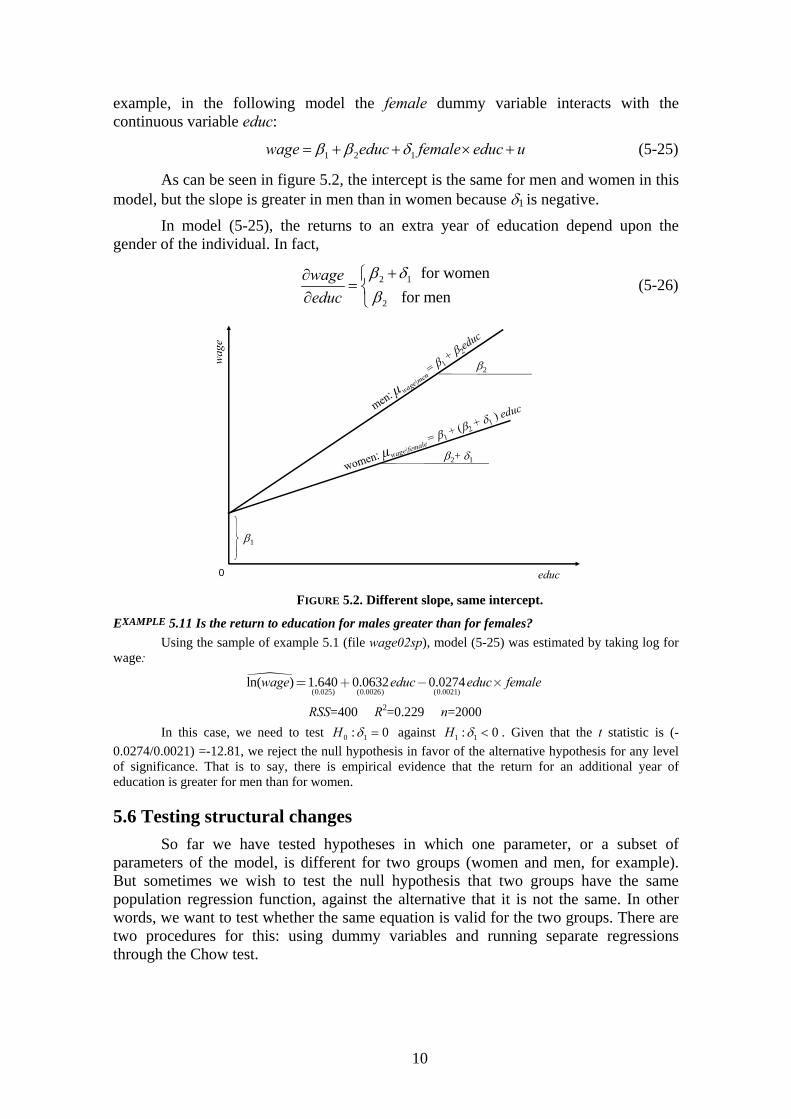
example, in the following model the female dummy variable interacts with the continuous variable educ:

1 2 1wage educ female educ u (5-25)

As can be seen in figure 5.2, the intercept is the same for men and women in this model, but the slope is greater in men than in women because 1 is negative.

In model (5-25), the returns to an extra year of education depend upon the gender of the individual. In fact,

2 1

2

for women

for men

wage

educ

(5-26)

FIGURE 5.2. Different slope, same intercept.

EXAMPLE 5.11 Is the return to education for males greater than for females?

Using the sample of example 5.1 (file wage02sp), model (5-25) was estimated by taking log for wage:

(0.025) (0.0026) (0.0021)

ln( ) 1.640 0.0632 0.0274wage educ educ female = + - ´

RSS=400 R2=0.229 n=2000

In this case, we need to test 0 1: 0H against 1 1: 0H . Given that the t statistic is (-

0.0274/0.0021) =-12.81, we reject the null hypothesis in favor of the alternative hypothesis for any level of significance. That is to say, there is empirical evidence that the return for an additional year of education is greater for men than for women.

5.6 Testing structural changes

So far we have tested hypotheses in which one parameter, or a subset of parameters of the model, is different for two groups (women and men, for example). But sometimes we wish to test the null hypothesis that two groups have the same population regression function, against the alternative that it is not the same. In other words, we want to test whether the same equation is valid for the two groups. There are two procedures for this: using dummy variables and running separate regressions through the Chow test.

wag

e

educ

2+ 1

0

1

2

11

5.6.1 Using dummy variables

In this procedure, testing for differences across groups consists in performing a joint significance test of the dummy variable, which distinguishes between the two groups and its interactions with all other independent variables. We therefore estimate the model with (unrestricted model) and without (restricted model) the dummy variable and all the interactions.

From the estimation of both equations we form the F statistic, either through the RSS or from the R2. In the following model for the determination of wages, the intercept and the slope are different for males and females:

1 1 2 2wage female educ female educ u (5-27)

The population regression function corresponding to this model is represented in figure 5.3. As can be seen, if female=1, we obtain

1 1 2 2( ) ( )wage educ u (5-28)

For women the intercept is 1 1 , and the slope 2 2 . For female=0, we

obtain equation (5-1). In this case, for men the intercept is 1 , and the slope 2 .

Therefore, 1 measures the difference in intercepts between men and women and, 2 measures the difference in the return to education between males and females. Figure 5.3 shows a lower intercept and a lower slope for women than for men. This means that women earn less than men at all levels of education, and the gap increases as educ gets larger; that is to say, an additional year of education shows a lower return for women than for men.

Estimating (5-27) is equivalent to estimating two wage equations separately, one for men and another for women. The only difference is that (5-27) imposes the same variance across the two groups, whereas separate regressions do not. This set-up is ideal, as we will see later on, for testing the equality of slopes, equality of intercepts, and equality of both intercepts and slopes across groups.

FIGURE 5.3. Different slope, different intercept.

EXAMPLE 5.12 Is the wage equation valid for both men and women?

If parameters 1 and 2 are equal to 0 in model (5-27), this will imply that the equation for wage determination is the same for men and women. In order to answer the question posed, we take (5-27), as

wag

e

educ

2+ 2

0

1

1 +

2

12

the unrestricted model but express wage in logs. The null and the alternative hypothesis will be the following:

0 1 2

1 0

: 0

: is not true

H

H H

Therefore, the restricted model is model (5-17). Using the same sample as in example 5.1 (file wage02sp), we have obtained the following estimation of models (5-27) and (5-17):

(0.030) (0.0546) (0.0030) (0.0054)

ln( ) 1.739 0.3319 0.0539 0.0027wage female educ educ female = - + - ´

RSS=393 R2=0.243 n=2000

(0.026) (0.0026)

ln( ) 1.657 0.0525wage educ= +

RSS=433 R2=0.166 n=2000

The F statistic takes the value

/ 433 393 / 2

/ ( ) 393 / (2000 4)R UR

UR

RSS RSS qF

RSS n k

102

It is clear that for any level of significance, the equations for men and women are different.

When we tested in example 5.1 whether there was discrimination in Spain against women (

0 1: 0H against 1 1: 0H ), it was assumed that the slope of educ (model (5-6)) is the same for men

and women. Now it is also possible to use model (5-27) to test the same null hypothesis, but assuming a different slope. Given that the t statistic is (-0.3319/0.0546)=-6.06, we reject the null hypothesis by using this more general model than the one in example 5.1.

In example 5.11 it was tested whether the coefficient 2 in model (5-25), taking log for wage, was 0, assuming that the intercept is the same for males and females. Now, if we take (5-27), taking log for wage, as the unrestricted model, we can test the same null hypothesis, but assuming that the intercept is different for males and females. Given that the t statistic is (0.0027/0.0054)=0.49, we cannot reject the null hypothesis which states that there is no interaction between gender and education.

EXAMPLE 5.13 Would urban consumers have the same pattern of behavior as rural consumers regarding expenditure on fish?

To answer this question, we formulate the following model which is taken as the unrestricted model:

1 1 2 2ln( ) ln( ) ln( )fish urban inc inc urban u (5-29)

The null and the alternative hypothesis will be the following:

0 1 2

1 0

: 0

: is not true

H

H H

The restricted model corresponding to this H0 is

1 2ln( ) ln( )fish inc u (5-30)

Using the sample of example 5.3 (file demand), models (5-29) and (5-30) were estimated:

(0.627) (1.095) (0.087) (0.152)

ln( ) 6.551 0.678 1.337 ln( ) 0.075ln( )fish urban inc inc urban=- + + - ´

RSS=1.123 R2=0.904 n=40

(0.542) (0.075)

ln( ) 6.224 1.302ln( )fish inc =- +

RSS=1.325 R2=0.887 n=40

The F statistic takes the value

/ 1.325 1.123 / 2

/ ( ) 1.123 / (40 4)R UR

UR

RSS RSS qF

RSS n k

3.24

If we look up in the F table for 2 df in the numerator and 35 df in the denominator for =0.10,

we find 0.10 0.102,36 2,35 2.46F F . As F>2.46 we reject 0H . However, as 0.05 0.05

2,36 2,35 3.27F F , we fail to

13

reject 0H in favour of H1 for =0.05 and, therefore, for =0.01. Conclusion: there is no strong evidence

that families living in rural areas have a different pattern of fish consumption than families living in rural areas.

Example 5.14 Has the productive structure of Spanish regions changed?

The question to be answered is specifically the following: Did the productive structure of Spanish regions change between 1995 and 2008? The problem posed is a problem of structural stability. To specify the model to be taken as a reference in the test, let us define the dummy y2008, which takes the value 1 if the year is 2008 and 0 if the year is 1995.

The reference model is a Cobb-Douglas model, which introduces additional parameters to collect the structural changes that may have occurred. Its expression is:

1 1 1 2 2 2ln( ) ln( ) ln( ) 2008 2008 ln( ) 2008 ln( )q k l y y k y l u (5-31)

It is easily seen, according to the definition of the dummy y2008, that the elasticities production/capital are different in the periods 1995 and 2008. Specifically, they take the following values:

(1995) 1 (2008) 1 2

ln( ) ln( ) +

ln( ) ln( )Q K Q K

Q Q

K K

In the case that 2 is equal to 0, then the elasticity of production/capital is the same in both periods.

Similarly, the production/labor elasticities for the two periods are given by

(1995) 1 (2008) 1 2

ln( ) ln( ) +

ln( ) ln( )Q K Q K

L L

K K

The intercept in the Cobb-Douglas is a parameter that measures efficiency. In model (5-31), the possibility that the efficiency parameter (PEF) is different in the two periods is considered. Thus

1 1 2(1995) (2008) + PEF PEF

If the parameters 1, 1 and 1 are zero in model (5-31), the production function is the same in both periods. Therefore, in testing structural stability of the production function, the null and alternative hypotheses are:

0 2 2 2

1 0

is not true

H

H H

(5-32)

Under the null hypothesis, the restrictions given in (5-32) lead to the following restricted model:

1 1 1ln( ) ln( ) ln( )q k l u (5-33)

The file prodsp contains information for each of the Spanish regions in 1995 and 2008 on gross value added in millions of euros (gdp), occupation in thousands of jobs (labor), and productive capital in millions of euros (captot). You can also find the dummy y2008 in that file.

The results of the unrestricted regression model (5-31) are shown below. It is evident that we cannot reject the null hypothesis that each of the coefficients 1, 1 and 1, taken individually, are 0, since none of the t statistics reaches 0.1 in absolute value.

(0.916) (0.185) (0.185)

(2.32) (0.419) (0.418)

ln( ) 0.0559 0.6743ln( ) 0.3291ln( )

0.1088 20108 0.0154 2008 ln( ) 0.0094 2008 ln( )

gva captot labor

y y captot y labor

+ +

- + ´ - ´

R2=0.99394 n=34

The results of the restricted model (5-33) are the following:

(0.200) (0.036) (0.042)

ln( ) 0.0690 0.6959ln( ) 0.311ln( )gva captot labor+ +

R2=0.99392 n=34

As can be seen, the R2 of the two models are virtually identical because they differ only from the fifth decimal. It is not surprising, therefore, that the F statistic for testing the null hypothesis (5-32) takes a value close to 0:

2 2

2

( ) / (0.99394 0.99392) / 30.0308

(1 0.99394) / (34 6)(1 ) / ( )UR R

UR

R R qF

R n k

14

Thus, the alternative hypothesis that there is structural change in the productive economy of the Spanish regions between 1995 and 2008 is rejected for any significance level.

5.6.2 Using separate regressions: The Chow test

This test was introduced by the econometrician Chow (1960). He considered the problem of testing the equality of two sets of regression coefficients. In the Chow test, the restricted model is the same as in the case of using dummy variables to distinguish between groups. The unrestricted model, instead of distinguishing the behaviour of the two groups by using dummy variables, consists simply of separate regressions. Thus, in the wage determination example, the unrestricted model consists of two equations:

11 21

12 22

:

:

female wage educ u

male wage educ u

(5-34)

If we estimate both equations by OLS, we can show that the RSS of the unrestricted model, RSSUR, is equal to the sum of the RSS obtained from the estimates for women, RSS1, and for men, RSS2. That is to say,

RSSUR=RSS1+RSS2

The null hypothesis states that the parameters of the two equations in (5-34) are equal. Therefore

11 120

21 22

1 0

:

: No

H

H H

By applying the null hypothesis to model (5-34), you get model (5-17), which is the restricted model. The estimation of this model for the whole sample is usually called the pooled (P) regression. Thus, we will consider that the RSSR and RSSP are equivalent expressions.

Therefore, the F statistic will be the following:

1 2

1 2

/

/ 2

PRSS RSS RSS kF

RSS RSS n k

(5-35)

It is important to remark that, under the null hypothesis, the error variances for the groups must be equal. Note that we have k restrictions: the slope coefficients (interactions) plus the intercept. Note also that in the unrestricted model we estimate two different intercepts and two different slope coefficients, and so the df of the model are n2k.

One important limitation of the Chow test is that under the null hypothesis there are no differences at all between the groups. In most cases, it is more interesting to allow partial differences between both groups as we have done using dummy variables.

The Chow test can be generalized to more than two groups in a natural way. From a practical point of view, to run separate regressions for each group to perform the test is probably easier than using dummy variables.

In the case of three groups, the F statistic in the Chow test will be the following:

15

1 2 3

1 2 3

( ) / 2

( ) / ( 3 )PRSS RSS RSS RSS k

FRSS RSS RSS n k

(5-36)

Note that, as a general rule, the number of the df of the numerator is equal to the (number of groups-1)k, while the number of the df of the denominator is equal to n minus (number of groups)k.

EXAMPLE 5.15 Another way to approach the question of wage determination by gender

Using the same sample as in example 5.1 (file wage02sp), we have obtained the estimation of the equations in (5-34), taking log for wage, for men and women, which taken together gives the estimation of the unrestricted model:

Female equation (0.042) (0.0041)

ln( ) 1.407 0.0566wage educ= +

RSS=104 R2=0.236 n=617

Male equation (0.031) (0.0032)

ln( ) 1.739 0.0539wage educ= +

RSS=289 R2=0.175 n=1383

The restricted model, estimated in example 5.4, has the same configuration as the equations in (5-34) but in this case refers to the whole sample. Therefore, it is the pooled regression corresponding to the restricted model. The F statistic takes the value

( ) / 433 (104 289) / 2

) / ( 2 ) (104 289) / (2000 2 2)P F M

F M

RSS RSS RSS kF

RSS RSS n k

102

The F statistic must be, and is, the same as in example 5.12. The conclusions are therefore the same.

EXAMPLE 5.16 Is the model of wage determination the same for different firm sizes?

In other examples the intercept, or the slope on education, was different for three different firm sizes (small, medium and large). Now we shall consider a completely different equation for each firm size. Therefore, the unrestricted model will be composed by three equations:

11 11 21

12 12 22

13 13 23

: ln( )

: ln( )

: ln( )

samall wage female edu u

medium wage female edu u

large wage female edu u

(5-37)

The null and the alternative hypothesis will be the following:

11 12 13

0 11 12 13

21 22 23

1 0

:

: No

H

H H

Given this null hypothesis, the restricted model is model (5-2).

The estimations of the three equations of (5-37), by using file wage02sp, are the following:

small (0.034) (0.031) (0.0038)

ln( ) 1.706 0.249 0.0396wage female educ = - +

RSS=121 R2=0.160 n=801

medium (0.051) (0.039) (0.0046)

ln( ) 1.934 0.422 0.0548wage female educ = - +

RSS =123 R2=0.302 n=590

large (0.046) (0.039) (0.0044)

ln( ) 1.749 0.303 0.0554wage female educ = - +

RSS =114 R2=0.273 n=609

The pooled regression has been estimated in example 5.1. The F statistic takes the value

16

( ) / 2

( ) / ( 3 )

393 (121 123 114) / 632.4

(121 123 114) / (2000 3 3)

P S M L

S M L

RSS RSS RSS RSS kF

RSS RSS RSS n k

For any level of significance, we reject that the equations for wage determination are the same for different firm sizes.

EXAMPLE 5.17 Is the Pinkham model valid for the four periods?

In example 5.5, we introduced time dummy variables and we tested whether the intercept was different for each period. Now, we are going to test whether the whole model is valid for the four periods considered. Therefore, the unrestricted model will be composed by four equations:

11 21 31 1

12 22 32 1

13 23 33 1

14 24 34

1907-1914

1915-1925

1926-1940

1941-1960

t t t t

t t t t

t t t t

t t

sales advexp sales u

sales advexp sales u

sales advexp sales u

sales advexp

1 t tsales u

(5-38)

The null and the alternative hypothesis will be the following:

11 12 13 14

0 21 22 23 24

31 32 33 34

1 0

:

: No

H

H H

Given this null hypothesis, the restricted model is the following model:

1 2 3 1 t t t tsales advexp sales u (5-39)

The estimations of the four equations of (5-38) are the following:

1

(603) (1.025) (0.425)1907-1914 64.84 0.9149 0.4630 36017 7 t tsales advexp sales SSR n-= + + = =

1(190) (0.557) (0.300)

1915-1925 221.5 0.1279 0.9319 400605 11t tsales advexp sales SSR n-= + + = =

1

(112) (0.115) (0.0827)1926-1940 446.8 0.4638 0.4445 201614 15t tsales advexp sales SSR n-= + + = =

1(134) (0.241) (0.111)

1941-1960 182.4 1.6753 0.3042 187332 20t tsales advexp sales SSR n-=- + + = =

The pooled regression, estimated in example 3.4, is the following:

1

(95.7) (0.156) (0.0915)138.7 0.3288 0.7593 2527215 53t tsales advexp sales SSR n-= + + = =

The F statistic takes the value

1 2 3 4

1 2 3 4

( ) / 3

( ) / ( 4 )

2527215 (36017 400605 201614 187332) / 99.16

(36017 400605 201614 187332) / (53 4 3)

PSSR SSR SSR SSR SSR kF

SSR SSR SSR SSR n k

For any level of significance, we reject that the model (5-39) is the same for the four periods considered.

Exercises

Exercise 5.1 Answer the following questions for a model with explanatory dummy variables:

a) What is the interpretation of the dummy coefficients? b) Why are not included in the model so many dummy variables as

categories there are?

17

Exercise 5.2 Using a sample of 560 families, the following estimations of demand for rental are obtained:

(0.11) (0.017) (0.026)ˆ 4.17 0.247 0.960i i iq p y

R2=0.371 n=560

(0.13) (0.030) (0.031) (0.120)ˆ 5.27 0.221 0.920 0.341i i i i iq p y d y

R2=0.380

where qi is the log of expenditure on rental housing of the ith family, pi is the logarithm of rent per m2 in the living area of the ith family, yi is the log of household disposable income of the ith family and di is a dummy variable that takes value one if the family lives in an urban area and zero in a rural area.

(The numbers in parentheses are standard errors of the estimators.)

a) Test the hypothesis that the elasticity of expenditure on rental housing with respect to income is 1, in the first fitted model.

b) Test whether the interaction between the dummy variable and income is significant. Is there a significant difference in the housing expenditure elasticity between urban and rural areas? Justify your answer.

Exercise 5.3 In a linear regression model with dummy variables, answer the following questions:

a) The meaning and interpretation of the coefficients of dummy variables in models with endogenous variable in logs.

b) Express how a model is affected when a dummy variable is introduced in a multiplicative way with respect to a quantitative variable.

Exercise 5.4 In the context of a multiple linear regression model,

a) What is a dummy variable? Give an example of an econometric model with dummy variables. Interpret the coefficients.

b) When is there perfect multicollinearity in a model with dummy variables?

Exercise 5.5 The following estimation is obtained using data for workers of a company: 500 50 200 00i i i iwage tenure college 1 male= + + +

where wage is the wage in euros per month, tenure is the number of years in the company, college is a dummy variable that takes value 1 if the worker is graduated from college and 0 otherwise and male is a dummy variable which takes value 1 if the worker is male and 0 otherwise.

a) What is the predicted wage for a male worker with six years of tenure and college education?

b) Assuming that all working women have college education and none of the male workers do, write a hypothetical matrix of regressors (X) for six observations. In this case, would you have any problem in the estimation of this model? Explain it.

c) Formulate a new model that allows to establish whether there are wage differentials between workers with primary, secondary and college education.

18

Exercise 5.6 Consider the following linear regression model:

1 1 2 2i i i i iy x d d u (1)

where y is the monthly salary of a teacher, x is the number of years of teaching experience y d1 y d2 are two dummy variables taking the following values:

1

1 if the teacher is male

0 otherwiseid

2

1 if the teacher is white

0 otherwiseid

a) What is the reference category in the model? b) Interpret 1 and 2. What is the expected salary for each of the possible

categories? c) To improve the explanatory power of the model, the following alternative

specification was considered:

1 1 2 2 3 1 2( )i i i i i i iy x d d d d u (2)

d) What is the meaning of the term 1 2( )i id d ? Interpret 3.

e) What is the expected salary for each of the possible categories in model (2)?

Exercise 5.7 Using a sample of 36 observations, the following results are obtained:

1 2 3(0.12) (0.34) (3.35) (0.07)

ˆ 1.10 0.96 4.56 0.34t t t ty x x x

2 2

1 1

ˆ ˆ109.24 20.22n n

t tt t

y y u

(The numbers in parentheses are standard errors of the estimators.)

a) Test the individual significance of the coefficient associated with x2. b) Calculate the coefficient of determination, R2, and explain its meaning. c) Test the joint significance of the model. d) Two additional regressions, with the same specification, were made for

the two categories A and B included in the sample (n1=21 y n2=15). In these estimates the following RSS were obtained: 11.09 y 2.17, respectively. Test if the behavior of the endogenous variable is the same in the two categories.

Exercise 5.8 To explain the time devoted to sport (sport), the following model was formulated

1 1 1 2sport female smoker age u b d j b+ + + + (1)

where sport is the minutes spent on sports a day, on average; female and smoker are dummy variables taking the value 1 if the person is a woman or smoker of at least five cigarettes per day, respectively.

a) Interpret the meaning of 1, 1j and 2.

b) What is the expected time spent on sports activities for all possible categories?

c) To improve the explanatory power of the model, the following alternative specification was considered:

1 1 1 1

2 2 2

depor mujer fumador mujer fumador

mujer edad fumador edad edad u

b d j gd j b

+ + + ´

+ ´ + ´ + + (2)

19

In model (2), what is the meaning of 1? What is the meaning of 2 and

2j ?

d) What are the possible marginal effects of sport with respect to age in the model (2)? Describe them.

Exercise 5.9 Using information for Spanish regions in 1995 and 2000, several production functions were estimated.

For the whole of the two periods, the following results were obtained:

ln( ) 5.72 0.26ln( ) 0.75ln( ) 1.14 0.11 ln( ) 0.05 ln( )q k l f f k f l= + + - + ´ - ´ (1) 2 20.9594 0.9510 0.9380 34R R RSS n

ln( ) 3.91 0.45ln( ) 0.60( )q k l= + + (2)

2 20.9567 0.9525 1.0007R R RSS

Moreover, the following models were estimated separately for each of the years:

1995 ln( ) 5.72 0.26ln( ) 0.75q k l= + + (3) 2 20.9527 0.9459 =0.6052R R RSS

2000 ln( ) 4.58 0.37 ln( ) 0.70q k l= + + (4) 2 20.9629 0.9555 =0.3331R R RSS

where q is output, k is capital, l is labor and f is a dummy variable that takes the value 1 for 1995 data and 0 for 2000.

a) Test whether there is structural change between 1995 and 2000. b) Compare the results of estimations (3) and (4) with estimation (1). c) Test the overall significance of model (1).

Exercise 5.10 With a sample of 300 service sector firms, the following cost function was estimated:

(0.025)

0.847 0.899 901.074 300i icost qty RSS n= + = =

where qtyi is the quantity produced.

The 300 firms are distributed in three big areas (100 in each one). The following results were obtained:

Area 1: 2

(0.038)ˆ1.053 0.876 0.457i icost qty s= + =

Area 2: 2

(0.096)ˆ3.279 0.835 3.154i icost qty s= + =

Area 3: 2

(0.10)ˆ5.279 0.984 4.255i icost qty s= + =

a) Calculate an unbiased estimation of 2 in the cost function for the sample of 300 firms.

b) Is the same cost function valid for the three areas?

Exercise 5.11 To study spending on magazines (mag), the following models have been formulated:

1 2 3 4ln( ) ln( )mag inc age male u (1)

1 2 3 4 5 6ln( ) ln( )mag inc age male prim sec u (2)

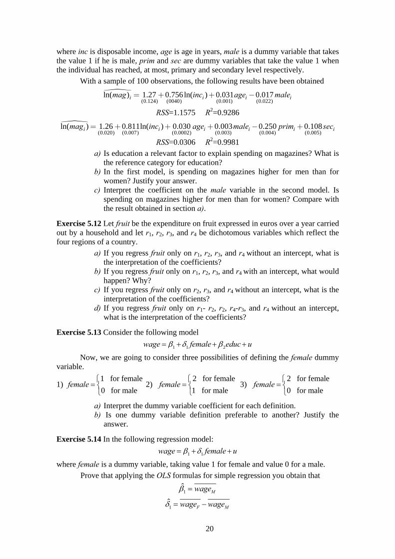
20

where inc is disposable income, age is age in years, male is a dummy variable that takes the value 1 if he is male, prim and sec are dummy variables that take the value 1 when the individual has reached, at most, primary and secondary level respectively.

With a sample of 100 observations, the following results have been obtained

(0.124) (0040) (0.001) (0.022)ln( ) 1.27 0.756 ln( ) 0.031 0.017i i i imag inc age male= + + -

RSS=1.1575 R2=0.9286

(0.020) (0.007) (0.0002) (0.003) (0.004) (0.005)ln( ) 1.26 0.811ln( ) 0.030 0.003 0.250 0.108i i i i i imag inc age male prim sec= + + + - +

RSS=0.0306 R2=0.9981

a) Is education a relevant factor to explain spending on magazines? What is the reference category for education?

b) In the first model, is spending on magazines higher for men than for women? Justify your answer.

c) Interpret the coefficient on the male variable in the second model. Is spending on magazines higher for men than for women? Compare with the result obtained in section a).

Exercise 5.12 Let fruit be the expenditure on fruit expressed in euros over a year carried out by a household and let r1, r2, r3, and r4 be dichotomous variables which reflect the four regions of a country.

a) If you regress fruit only on r1, r2, r3, and r4 without an intercept, what is the interpretation of the coefficients?

b) If you regress fruit only on r1, r2, r3, and r4 with an intercept, what would happen? Why?

c) If you regress fruit only on r2, r3, and r4 without an intercept, what is the interpretation of the coefficients?

d) If you regress fruit only on r1- r2, r2, r4-r3, and r4 without an intercept, what is the interpretation of the coefficients?

Exercise 5.13 Consider the following model

1 1 2wage female educ u

Now, we are going to consider three possibilities of defining the female dummy variable.

1) 1 for female

0 for malefemale

2) 2 for female

1 for malefemale

3) 2 for female

0 for malefemale

a) Interpret the dummy variable coefficient for each definition. b) Is one dummy variable definition preferable to another? Justify the

answer.

Exercise 5.14 In the following regression model:

1 1wage female u

where female is a dummy variable, taking value 1 for female and value 0 for a male.

Prove that applying the OLS formulas for simple regression you obtain that

1̂ Mwage

1̂ F Mwage wage

21

where F indicates female and M male.

In order to obtain a solution, consider that in the sample there are n1 females and n2 males: the total sample is n= n1+n2.

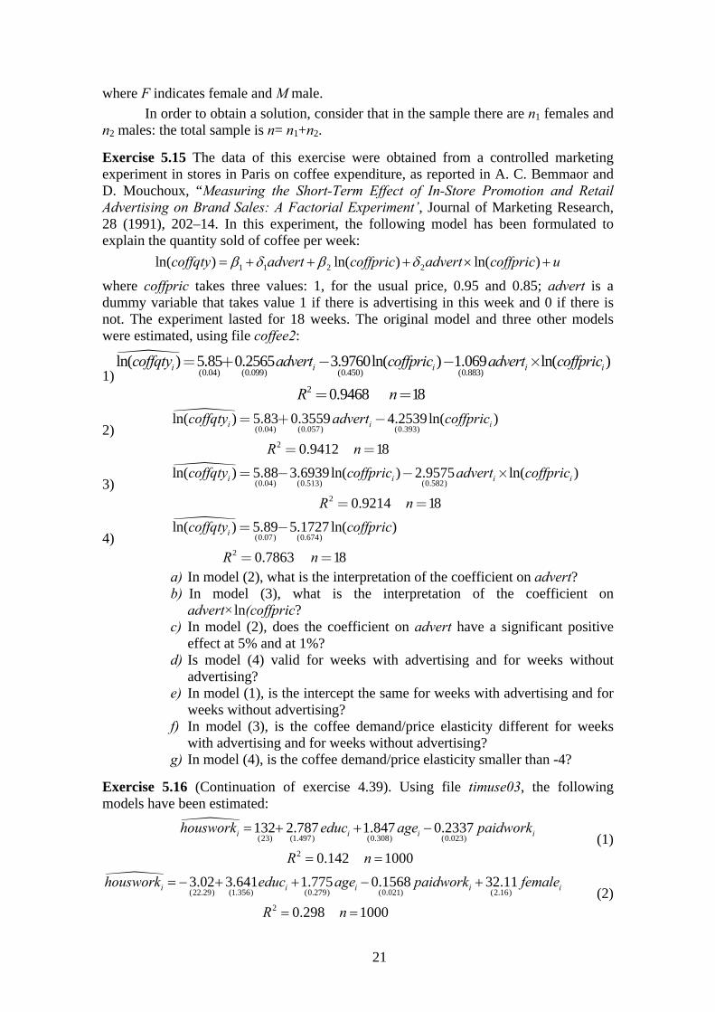
Exercise 5.15 The data of this exercise were obtained from a controlled marketing experiment in stores in Paris on coffee expenditure, as reported in A. C. Bemmaor and D. Mouchoux, “Measuring the Short-Term Effect of In-Store Promotion and Retail Advertising on Brand Sales: A Factorial Experiment’, Journal of Marketing Research, 28 (1991), 202–14. In this experiment, the following model has been formulated to explain the quantity sold of coffee per week:

1 1 2 2ln( ) ln( ) ln( )coffqty advert coffpric advert coffpric u

where coffpric takes three values: 1, for the usual price, 0.95 and 0.85; advert is a dummy variable that takes value 1 if there is advertising in this week and 0 if there is not. The experiment lasted for 18 weeks. The original model and three other models were estimated, using file coffee2:

1)

(0.04) (0.099) (0.450) (0.883)

2

ln( ) 5.85 0.2565 3.9760ln( ) 1.069 ln( )

0.9468 18

i i i i icoffqty advert coffpric advert coffpric

R n

= + - - ´

= =

2)

(0.04) (0.057) (0.393)

2

ln( ) 5.83 0.3559 4.2539ln( )

0.9412 18

i i icoffqty advert coffpric

R n

= + -

= =

3)

(0.04) (0.513) (0.582)

2

ln( ) 5.88 3.6939ln( ) 2.9575 ln( )

0.9214 18

i i i icoffqty coffpric advert coffpric

R n

= - - ´

= =

4)

(0.07) (0.674)

2

ln( ) 5.89 5.1727 ln( )

0.7863 18

icoffqty coffpric

R n

= -

= =

a) In model (2), what is the interpretation of the coefficient on advert? b) In model (3), what is the interpretation of the coefficient on

advert×ln(coffpric? c) In model (2), does the coefficient on advert have a significant positive

effect at 5% and at 1%? d) Is model (4) valid for weeks with advertising and for weeks without

advertising? e) In model (1), is the intercept the same for weeks with advertising and for

weeks without advertising? f) In model (3), is the coffee demand/price elasticity different for weeks

with advertising and for weeks without advertising? g) In model (4), is the coffee demand/price elasticity smaller than -4?

Exercise 5.16 (Continuation of exercise 4.39). Using file timuse03, the following models have been estimated:

(23) (1.497) (0.308) (0.023)

2

132 2.787 1.847 0.2337

0.142 1000

i i i ihouswork educ age paidwork

R n

(1)

(22.29) (1.356) (0.279) (0.021) (2.16)

2

3.02 3.641 1.775 0.1568 32.11

0.298 1000

i i i i ihouswork educ age paidwork female

R n

(2)

22

(35.18) (2.352) (0.502) (0.032) (8.15)

(0.546) (0.112) (0.009)

2

8.04 4.847 1.333 0.0871 32.75

0.1650 0.1019 0.02625

0.306 10

i i i i i

i i i i i i

houswork educ age paidwork female

educ female age female paidwork female

R n

00

(3)

a) In model (1), is there a statistically significant tradeoff between time devoted to paid work and time devoted to housework?

b) All other factors being equal and taking as a reference model (2), is there evidence that women devote more time to housework than men?

c) Compare the R2 of models (1) and (2). What is your conclusion? d) In model (3), what is the marginal effect of time devoted to housework

with respect to time devoted to paid work? e) Is interaction between paidwork and gender significant? f) Are the interactions between gender and the quantitative variables of the

model jointly significant?

Exercise 5.17 Using data from Bolsa de Madrid (Madrid Stock Exchange) on November 19, 2011 (file bolmad11), the following models have been estimated:

(0.243) (0.179) (0.0369)

ln( ) 1.784 0.6998 35 0.6749ln( )i i imarktval ibex bookval= + + (1)

RSS=35.69 R2=0.8931 n=92

(0.275) (0.778) (0.0423)

(0.088)

ln( ) 1.828 0.4236 35 0.6678ln( )

0.0310 35 ln( )

i i i

i i

marktval ibex bookval

ibex bookval

= + +

+ ´ (2)

RSS=35.622 R2=0.8933 n=92

(0.310) (0.785) (0.0405)

(0.089) (0.236) (0.221)

(0.263) (0.207)

ln( ) 2.323 0.1987 35 0.6688ln( )

0.0369 35 ln( ) 0.6613 0.6698

0.1931 0.3895 0.

i i i

i i i i

i i

marktval ibex bookval

ibex bookval services consump

energy industry

= + +

+ ´ - -

- - -(0.324)7020 iitt

(3)

RSS=30.781 R2=0.9078 n=92

(0.234) (0.0305)

ln( ) 1.366 0.7658ln( )i imarktval bookval= + (4)

RSS=41.625 R2=0.8753 n=92

For finance=1 (0.560) (0.0702)

ln( ) 0.558 0.9346ln( )i imarkval bookval= + (5)

RSS=2.7241 R2=0.9415 n=13

where

- marktval is the capitalization value of a company.

- bookval is the book value of a company.

- ibex35 is a dummy variable that takes the value 1 if the corporation is included in the selective Ibex 35.

- services, consumption, energy, industry and itc (information technology and communication) are dummy variables. Each of them takes the value 1 if the corporation is classified in this sector in Bolsa de Madrid. The category of reference is finance.

23

a) In model (1), what is interpretation of the coefficient on ibex35? b) In model (1), is the marktval/bookval elasticity equal to 1? c) In model (2), is the elasticity marktval/bookval the same for all

corporations included in the sample? d) Is model (4) valid both for corporations included in ibex 35 and for

corporations excluded? e) In model (3), what is interpretation of the coefficient on consump? f) Is the coefficient on consump significatively negative? g) Is the introduction of dummy variables for different sectors statistically

justifiable? h) Is the marktval/bookval elasticity for the financial sector equal to 1?

Exercise 5.18 (Continuation óf exercise 4.37). Using file rdspain, the equations which appear in the attached table have been estimated.

The following variables appear in the table:

- rdintens is expenditure on research and development (R&D) as a percentage of sales,

- sales are measured in millions of euros,

- exponsal is exports as a percentage of sales;

- medtech and hightech are two dummy variables which reflects if the firm belongs to a medium or a high technology sector. The reference category corresponds to the firms with low technology,

- workers is the number of workers.

24

(1)

rdintens (2)

rdintens (3)

rdintens

(4) (5) (6) rdintens rdintens rdintens for hightech=1 for medtech=1 for lowtech=1exponsal 0.0136 0.0101 0.00968 0.00584 0.0116 0.00977 (0.00195) (0.00193) (0.00189) (0.00792) (0.00300) (0.00169) workers 0.000433 0.000392 0.000394 0.00196 0.0000563 0.000393 (0.0000740) (0.0000725) (0.000208) (0.000338) (0.0000815) (0.000121) hightech 1.448 0.976 (0.141) (0.151) medtech 0.361 0.472 (0.109) (0.112) hightech× 0.00153 workers (0.000271) medtech× -0.000326 workers (0.000222) intercept 0.394 0.137 0.143 1.211 0.577 0.142 (0.0598) (0.0691) (0.0722) (0.313) (0.103) (0.0443) n 1983 1983 1983 296 616 1071R2 0.0507 0.0986 0.138 0.113 0.0278 0.0459RSS 9282.7 8815.0 8425.3 4409.0 2483.6 1527.5F 52.90 54.06 52.90 18.71 8.776 25.72df_n 2 4 6 2 2 2df_d 1980 1978 1976 293 613 1068

Standard errors in parentheses

a) In model (2), all other factors being equal, is there evidence that expenditure on research and development (expressed as a percentage of sales) in high technology firms is greater than in low technology firms? How strong is the evidence?

b) In model (2), all other factors being equal, is there evidence that rdintens in medium technology firms is equal to low technology firms? How strong is the evidence?

c) Taking as reference model (2), if you had to test the hypothesis that rdintens in high technology firms is equal to medium technology firms, formulate a model that allows you to test this hypothesis without using information on covariance matrix of the estimators

d) Is the influence of workers on rdintens associated with the level of technology in the firms?

e) Is the model (1) valid for all firms regardless of their technological level?

Exercise 5.19 To explain the overall satisfaction of people (stsfglo), the following model were estimated using data from the file hdr2010:

(0.584) (0.00000617) (0.009)

2

0.375 0.0000207 0.0858

0.642 144

i i istsfglo gnipc lifexpec

R n

(1)

25

(0.897) (0.00000572) (0.18)

(0.179) (0.259)

2

2.911 0.0000381 1.215

1.215 0.7901

0.748 144

i i i

i i

stsfglo gnipc lifexpec

dlatam dafrica

R n

(2)

(1.014) (0.000006) (0.0147) (0.177)

(1.712) (0.0000456) (0.0295)

2

1.701 0.0000327 0.0527 1.166

3.096 0.0000673 0.0699

0.760

i i i i

i i i i i

stsfglo gnipc lifexpec dlatam

dafrica gnipc dafrica lifexpec dafrica

R

144 n

(3)

where

- gnipc is gross national income per capita expressed in PPP 2008 US dollar terms,

- lifexpec is life expectancy at birth, i.e., number of years a newborn infant could be expected to live,

- dafrica is a dummy variable that takes value 1 if the country is in Africa,

- dlatam is a dummy variable that takes value 1 if the country is in Latin America.

a) In model (2), what is the interpretation of the coefficients on dlatam and dafrica?

b) In model (2), do dlatam and dafrica individually have a significant positive influence on global satisfaction?

c) In model (2), do dlatam and dafrica have a joint influence on global satisfaction?

d) Is the influence of life expectancy on global satisfaction smaller in Africa than in other regions of the world?

e) Is the influence of the variable gnipc greater in Africa than in other regions of the world at 10%?

f) Are the interactions of people living in Africa and the variables gnipc and lifexpec jointly significant?

Exercise 5.20 The equations which appear in the attached table have been estimated using data from the file timuse03. This file contains 1000 observations corresponding to a random subsample extracted from the time use survey for Spain carried out in 2002-2003.

The following variables appear in the table:

- educ is years of education attained,

- sleep, paidwork and unpaidwrk are measured in minutes per day,

- female, workday (Monday to Friday), spaniard and houswife are dummy variables.

a) In model (1), is there a statistically significant tradeoff between time devoted to paid work and time devoted to sleep?

b) In model (1), is the coefficient on unpaidwk statistically significant? c) In model (1), is there evidence that women sleep more than men? d) In model (2), are workday and spaniard individually significant? Are

they jointly significant? e) Is the coefficient on housewife statistically significant?

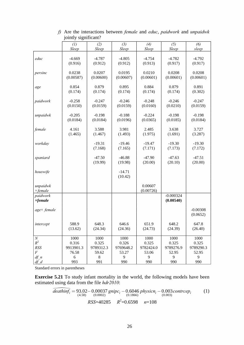
26

f) Are the interactions between female and educ, paidwork and unpaidwk jointly significant?

(1) (2) (3) (4) (5) (6) Sleep Sleep Sleep Sleep Sleep sleep

educ -4.669 -4.787 -4.805 -4.754 -4.782 -4.792 (0.916) (0.912) (0.912) (0.913) (0.917) (0.917)

persinc 0.0238 0.0207 0.0195 0.0210 0.0208 0.0208 (0.00587) (0.00600) (0.00607) (0.00601) (0.00601) (0.00601)

age 0.854 0.879 0.895 0.884 0.879 0.891 (0.174) (0.174) (0.174) (0.174) (0.174) (0.302)

paidwork -0.258 -0.247 -0.246 -0.248 -0.246 -0.247 (0.0150) (0.0159) (0.0159) (0.0160) (0.0210) (0.0159)

unpaidwk -0.205 -0.198 -0.188 -0.224 -0.198 -0.198 (0.0184) (0.0184) (0.0196) (0.0365) (0.0185) (0.0184)

female 4.161 3.588 3.981 2.485 3.638 3.727 (1.465) (1.467) (1.493) (1.975) (1.691) (3.287)

workday -19.31 -19.46 -19.47 -19.30 -19.30 (7.168) (7.165) (7.171) (7.173) (7.172)

spaniard -47.50 -46.88 -47.90 -47.63 -47.51 (19.99) (19.98) (20.00) (20.10) (20.00)

houswife -14.71 (10.42)

unpaidwk 0.00607 ×female (0.00726) paidwork -0.000324 ×female (0.00540)

age× female -0.00308 (0.0652)

intercept 588.9 648.3 646.6 651.9 648.2 647.8 (13.62) (24.34) (24.36) (24.73) (24.39) (26.40)

N 1000 1000 1000 1000 1000 1000 R2 0.316 0.325 0.326 0.325 0.325 0.325 RSS 9913901.3 9789312.3 9769648.2 9782424.0 9789276.9 9789290.3 F 76.58 59.62 53.27 53.06 52.95 52.95 df_n 6 8 9 9 9 9 df_d 993 991 990 990 990 990

Standard errors in parentheses

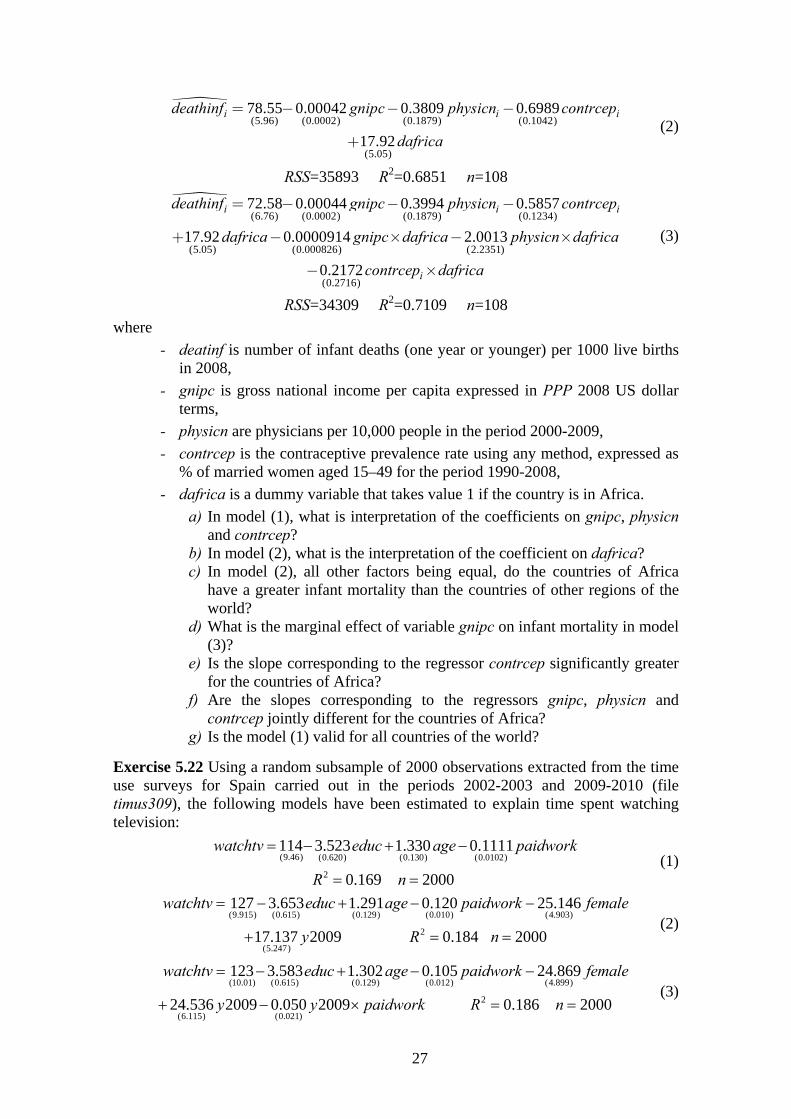
Exercise 5.21 To study infant mortality in the world, the following models have been estimated using data from the file hdr2010:

(4.58) (0.0002) (0.1866) (0.003)

93.02 0.00037 0.6046 0.003i i i ideathinf gnipc physicn contrcep= - - - (1)

RSS=40285 R2=0.6598 n=108

27

(5.96) (0.0002) (0.1879) (0.1042)

(5.05)

78.55 0.00042 0.3809 0.6989

17.92

i i ideathinf gnipc physicn contrcep

dafrica

= - - -

+ (2)

RSS=35893 R2=0.6851 n=108

(6.76) (0.0002) (0.1879) (0.1234)

(5.05) (0.000826) (2.2351)

(0.2716)

72.58 0.00044 0.3994 0.5857

17.92 0.0000914 2.0013

0.2172

i i i

i

deathinf gnipc physicn contrcep

dafrica gnipc dafrica physicn dafrica

contrcep dafr

= - - -

+ - ´ - ´

- ´ ica

(3)

RSS=34309 R2=0.7109 n=108

where

- deatinf is number of infant deaths (one year or younger) per 1000 live births in 2008,

- gnipc is gross national income per capita expressed in PPP 2008 US dollar terms,

- physicn are physicians per 10,000 people in the period 2000-2009,

- contrcep is the contraceptive prevalence rate using any method, expressed as % of married women aged 15–49 for the period 1990-2008,

- dafrica is a dummy variable that takes value 1 if the country is in Africa.

a) In model (1), what is interpretation of the coefficients on gnipc, physicn and contrcep?

b) In model (2), what is the interpretation of the coefficient on dafrica? c) In model (2), all other factors being equal, do the countries of Africa

have a greater infant mortality than the countries of other regions of the world?

d) What is the marginal effect of variable gnipc on infant mortality in model (3)?

e) Is the slope corresponding to the regressor contrcep significantly greater for the countries of Africa?

f) Are the slopes corresponding to the regressors gnipc, physicn and contrcep jointly different for the countries of Africa?

g) Is the model (1) valid for all countries of the world?

Exercise 5.22 Using a random subsample of 2000 observations extracted from the time use surveys for Spain carried out in the periods 2002-2003 and 2009-2010 (file timus309), the following models have been estimated to explain time spent watching television:

(9.46) (0.620) (0.130) (0.0102)

2

114 3.523 1.330 0.1111

0.169 2000

watchtv educ age paidwork

R n

(1)

(9.915) (0.615) (0.129) (0.010) (4.903)

2

(5.247)

127 3.653 1.291 0.120 25.146

17.137 2009 0.184 2000

watchtv educ age paidwork female

y R n

(2)

(10.01) (0.615) (0.129) (0.012) (4.899)

2

(6.115) (0.021)

123 3.583 1.302 0.105 24.869

24.536 2009 0.050 2009 0.186 2000

watchtv educ age paidwork female

y y paidwork R n

(3)

28

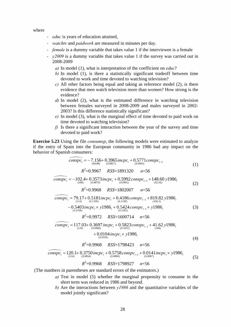
where

- educ is years of education attained,

- watchtv and paidwork are measured in minutes per day.

- female is a dummy variable that takes value 1 if the interviewee is a female

- y2009 is a dummy variable that takes value 1 if the survey was carried out in 2008-2009

a) In model (1), what is interpretation of the coefficient on educ? b) In model (1), is there a statistically significant tradeoff between time

devoted to work and time devoted to watching television? c) All other factors being equal and taking as reference model (2), is there

evidence that men watch television more than women? How strong is the evidence?

d) In model (2), what is the estimated difference in watching television between females surveyed in 2008-2009 and males surveyed in 2002-2003? Is this difference statistically significant?

e) In model (3), what is the marginal effect of time devoted to paid work on time devoted to watching television?

f) Is there a significant interaction between the year of the survey and time devoted to paid work?

Exercise 5.23 Using the file consumsp, the following models were estimated to analyze if the entry of Spain into the European community in 1986 had any impact on the behavior of Spanish consumers:

1(84.88) (0.0857) (0.0903)

7.156 0.3965 0.5771t t tconspc incpc conspc (1)

R2=0.9967 RSS=1891320 n=56

1(108) (0.0879) (0.0901) (92.56)

102.4 0.3573 0.5992 148.60 1986t t t tconspc incpc conspc y (2)

R2=0.9968 RSS=1802007 n=56

1

(114) (0.1100) (0.1199) (456.3)

1(0.2338) (0.2182)

79.17 0.5181 0.4186 819.82 1986

0.5403 1986 0.5424 1986

t t t t

t t t t

conspc incpc conspc y

incpc y conspc y

(3)

R2=0.9972 RSS=1600714 n=56

1

(118) (0.0968) (0.1051) (348)

(0.0326)

117.03 0.3697 0.5823 41.62 1986

0.0104 1986

t t t t

t t

conspc incpc conspc y

incpc y

(4)

R2=0.9968 RSS=1798423 n=56

1(114) (0.0854) (0.0890) (0.0087)

120.1 0.3750 0.5758 0.0141 1986t t t t tconspc incpc conspc incpc y (5)

R2=0.9968 RSS=1798927 n=56

(The numbers in parentheses are standard errors of the estimators.)

a) Test in model (5) whether the marginal propensity to consume in the short term was reduced in 1986 and beyond.

b) Are the interactions between y1986 and the quantitative variables of the model jointly significant?

29

c) Test whether there was a structural change in the consumption function in 1986.

d) Test whether the coefficient on conspct-1 changed in 1986 and beyond. e) Was there a gap between consumption before 1986, with respect to 1986

and beyond?