5 ELASTICITYANDITS APPLICATIONS - … · 5 ELASTICITYANDITS APPLICATIONS ... Learn the meaning of the concept of elasticity ... Distinguish between the price elasticity of demand

5 ELASTICITY AND ITSAPPLICATIONS

LEARNING OBJECTIVES

In this chapter you will:

• Learn the meaning of the concept of elasticity

• Learn the meaning of the elasticity of supply

• Examine what determines the elasticity of supply

• Apply the concept of elasticity to price, to both supplyand demand, to income and demand and therelationship between the changing prices of differentproducts on demand

• Examine what determines the elasticity of demand

• Understand the relevance of elasticity to totalexpenditure and total revenue

• Apply the concept of elasticity in two different markets

After reading this chapter you should be able to:

• Calculate elasticity using the midpoint method

• Calculate the price elasticity of supply

• Distinguish between an inelastic and elastic supplycurve

• Distinguish between the price elasticity of demand fornecessities and luxuries

• Calculate different elasticities – price, income and cross

• Demonstrate the impact of the price elasticity ofdemand on total expenditure and total revenue underconditions of different demand elasticities

87

ELASTICITY AND ITS APPLICATION

For businesses, the price they charge for the products they produce is a vital part of theirproduct positioning – what the product offering is in relation to competitors. We haveseen in Chapter 4 how markets are dynamic and that price acts as a signal to both sellersand buyers; when prices change, the signal is altered and producer and consumer behav-iour changes.

Imagine yourself as a producer of silicon chips for use in personal computers, laptopsand a variety of other electronic devices. Because you earn all your income from sellingsilicon chips, you devote much effort to making your factory as productive as it can be.You monitor how production is organized, staff recruitment and motivation levels, checksuppliers for cost effectiveness and quality, and study the latest advances in technology.You know that the more chips you manufacture, the more you will have available to sell,and the higher will be your income (assuming you sell them) and your standard ofliving.

One day a local university announces a major discovery. Scientists have devised a newmaterial to produce chips which would help to increase computing power by 50 per cent.How should you react to this news? Should you use the new material? Does this discov-ery make you better off or worse off than you were before? In this chapter we will seethat these questions can have surprising answers. The surprise will come from applyingthe most basic tools of economics – supply and demand – to the market for computerchips.

In any competitive market, such as the market for computer chips, the upward slop-ing supply curve represents the behaviour of sellers, and the downward sloping demandcurve represents the behaviour of buyers. The price of the good adjusts to bring thequantity supplied and quantity demanded of the good into balance. To apply this basicanalysis to understand the impact of the scientists’ discovery, we must first develop onemore tool: the concept of elasticity also referred to as price sensitivity. We know fromChapter 4 that when price rises, demand falls and supply rises. What we did not discussin the chapter was how far demand and supply change in response to changes in price –in other words, how sensitive supply and demand is to a change in prices. When study-ing how some event or policy affects a market, we can discuss not only the direction ofthe effects but their magnitude as well. Elasticity, a measure of how much buyers andsellers respond to changes in market conditions, allows us to analyse supply and demandwith greater precision.

PRICE ELASTICITY OF SUPPLY

When we introduced supply in Chapter 4, we noted that producers of a good offer to sellmore of it when the price of the good rises, when their input prices fall or when theirtechnology improves. To turn from qualitative to quantitative statements about quantitysupplied, we use the concept of elasticity.

The Price Elasticity of Supply and its Determinants

The law of supply states that higher prices raise the quantity supplied. The price elastic-ity of supply measures how much the quantity supplied responds to changes in theprice. Supply of a good is said to be elastic (or price sensitive) if the quantity suppliedresponds substantially to changes in the price. Supply is said to be inelastic (or priceinsensitive) if the quantity supplied responds only slightly to changes in the price.

The price elasticity of supply depends on the flexibility of sellers to change theamount of the good they produce. For example, seafront property has an inelastic supply

elasticity a measure of theresponsiveness of quantity demanded orquantity supplied to one of itsdeterminants

price elasticity of supply ameasure of how much the quantitysupplied of a good responds to a changein the price of that good, computed asthe percentage change in quantitysupplied divided by the percentagechange in price

88 Part 2 Microeconomics – the Market System

because it is almost impossible to produce more of it quickly – supply is not very sensi-tive to changes in price. By contrast, manufactured goods, such as books, cars and televi-sion sets, have relatively elastic supplies because the firms that produce them can runtheir factories longer in response to a higher price – supply is sensitive to changes inprice.

Elasticity can take any value greater than or equal to zero. The closer to zero the moreinelastic, and the closer to infinity the more elastic. We will look at the determinants ofsupply first and then look in more detail at how elasticity is computed.

The Determinants of Price Elasticity of Supply

The Time Period In most markets, a key determinant of the price elasticity of sup-ply is the time period being considered. Supply is usually more elastic in the long runthan in the short run. We can further distinguish between the short run and the veryshort run. Over very short periods of time, firms may find it impossible to respond to achange in price by changing output. In the short run firms cannot easily change the sizeof their factories or productive capacity to make more or less of a good but may havesome flexibility. For example, it might take a month to employ new labour but afterthat time some increase in output can be accommodated. Overall, in the short run, thequantity supplied is not very responsive to the price. By contrast, over longer periods,firms can build new factories or close old ones, hire new staff and buy in more capitaland equipment. In addition, new firms can enter a market and old firms can shut down.Thus, in the long run, the quantity supplied can respond substantially to price changes.

Productive Capacity Most businesses, in the short run, will have a finite capacity– an upper limit to the amount that they can produce at any one time determined by theamount of factor inputs they possess. How far they are using this capacity depends, inturn, on the state of the economy. In periods of strong economic growth, firms may beoperating at or near full capacity. If demand is rising for the product they produce andprices are rising, it may be difficult for the firm to expand output to meet this newdemand and so supply may be inelastic.

When the economy is growing slowly or is contracting, some firms may find theyhave to cut back output and may only be operating at 60 per cent of full capacity. Inthis situation, if demand later increased and prices started to rise, it may be much easierfor the firm to expand output relatively quickly and so supply would be more elastic.

The Size of the Firm/Industry It is possible that as a general rule, supply maybe more elastic in smaller firms or industries than in larger ones. For example, consider asmall independent furniture manufacturer. Demand for its products may rise and inresponse the firm may be able to buy in raw materials (wood, for example), to meetthis increase in demand. Whilst the firm will incur a cost in buying in this timber, it isunlikely that the unit cost for the material will increase. Compare this to a situationwhere a steel manufacturer increases its purchase of raw materials (iron ore, for exam-ple). Buying large quantities of iron ore on global commodity markets can drive up unitprice and, by association, unit costs.

A study of the coffee industry in Papua New Guinea1 found that the price elasticity ofsupply of smallholders was around 0.23 whereas that for large estates was much moreinelastic at 0.04. The study suggested that these figures compared well to estimatesderived in previous studies.

The response of supply to changes in price in large firms/industries, therefore, may beless elastic than in smaller firms/industries. This is also related to the number of firms in

1http://www.une.edu.au/bepp/working-papers/ag-res-econ/occasional-papers/agecop3.pdf

Chapter 5 Elasticity and its Applications 89

the industry – the more firms there are in the industry the easier it is to increase supply,other things being equal.

The Mobility of Factors of Production Consider a farmer whose land is cur-rently devoted to producing wheat. A sharp rise in the price of rape seed might encour-age the farmer to switch use of land from wheat to rape seed relatively easily. Themobility of the factor of production land, in this case, is relatively high and so supplyof rape seed may be relatively elastic.

A number of multinational firms that have plants in different parts of the world nowbuild each plant to be identical. What this means is that if there is disruption to oneplant the firm can more easily transfer operations to another plant elsewhere and con-tinue production ‘seamlessly’. Car manufacturers provide another example of this inter-changeability of parts and operations. The chassis, for example, may be identical across arange of branded car models. This is the case with some Audi, Volkswagen, Seat andSkoda models. This means that the supply may be more elastic as a result.

Compare this to the supply of highly skilled oncology consultants. An increase in thewages of oncology consultants (suggesting a shortage exists) will not mean that a renalconsultant or other doctors can suddenly switch to take advantage of the higher wages andincrease the supply of oncology consultants. In this example, the mobility of labour to switchbetween different uses is limited and so the supply of these specialist consultants is likely tobe relatively inelastic.

Ease of Storing Stock/Inventory In some firms, stocks can be built up toenable the firm to respond more flexibly to changes in prices. In industries where inven-tory build-up is relatively easy and cheap, the price elasticity of supply is more elasticthan in industries where it is much harder to do this. Consider the fresh fruit industry,for example. Storing fresh fruit is not easy because it is perishable and so the price elas-ticity of supply in this industry may be more inelastic.

Different cars? Different brands maybe but there are more similarities to these two cars thanthere are differences.

MAKSIM

TOOME/SHUTTERSTOCK

MAKSIM

TOOME/SHUTTERSTOCK


Computing the Price Elasticity of Supply

Now that we have discussed the price elasticity of supply in general terms, let’s be moreprecise about how it is measured. Economists compute the price elasticity of supply asthe percentage change in the quantity supplied divided by the percentage change in theprice. That is:

Price elasticity of supply ¼ Percentage change in quantity suppliedPercentage change in price

For example, suppose that an increase in the price of milk from €2.85 to €3.15 a litreraises the amount that dairy farmers produce from 90 000 to 110 000 litres per month.Using the midpoint method, we calculate the percentage change in price as:

Percentage change in price ¼ ð3:15� 2:85Þ=3:00� 100 ¼ 10%

Similarly, we calculate the percentage change in quantity supplied as:

Percentage change in quantity supplied ¼ ð110 000� 90 000Þ=100 000� 100 ¼ 20%

In this case, the price elasticity of supply is:

Price elasticity of supply ¼ 20%10%

¼ 2

In this example, the elasticity of 2 reflects the fact that the quantity supplied movesproportionately twice as much as the price.

The Midpoint Method of Calculating Percentage Changes

and Elasticities

If you try calculating the price elasticity of supply between two points on a supply curve,you will quickly notice an annoying problem: the elasticity for a movement from point Ato point B seems different from the elasticity for a movement from point B to point A.For example, consider these numbers:

Point A : Price ¼ €4 Quantity Supplied ¼ 80Point B : Price ¼ €6 Quantity Supplied ¼ 125

Going from point A to point B, the price rises by 50 per cent – the change in pricedivided by the original price � 100 (2/4 � 100) � and the quantity rises by 56.25 percent – the change in quantity supplied divided by the original supply � 100 (45/80 �100) � indicating that the price elasticity of supply is 56.25/50, or 1.125. By contrast,going from point B to point A, the price falls by 33 per cent (2/6 � 100), and thequantity falls by 36 per cent (45/125 � 100), indicating that the price elasticity of sup-ply is 36/33, or 1.09.

Note, in the working above we have rounded the fall in price to the nearest wholenumber (33 per cent). If we had not used this rounding, the price elasticity of supplywould be:

85� 125125

� �4� 66

� � ¼ 1:08


One way to avoid this problem is to use the midpoint method for calculating elastici-ties. In the example above we used a standard way to compute a percentage change –divide the change by the initial level and multiply by 100. By contrast, the midpointmethod computes a percentage change by dividing the change by the midpoint (or aver-age) of the initial and final levels. For instance, €5 is the midpoint of €4 and €6. There-fore, according to the midpoint method, a change from €4 to €6 is considered a 40 percent rise, because ((6 � 4)/5) � 100 ¼ 40. Similarly, a change from €6 to €4 is considered a40 per cent fall ((4 � 6)/5) � 100 ¼ �40. Looking at the quantity, moving from Point A toPoint B gives (125 � 80)/102.5 � 100 ¼ 43.9 per cent and for a price fall (80 � 125)/102.5� 100 ¼ �43.9 per cent.

Because the midpoint method gives the same answer regardless of the direction ofchange (as indicated by the negative sign), it is often used when calculating price elastic-ities between two points. In our example, the midpoint between point A and point B is:

Midpoint : Price ¼ €5 Quantity ¼ 102:5

According to the midpoint method, when going from point A to point B, the pricerises by 40 per cent, and the quantity rises by 43.9 per cent. Similarly, when going frompoint B to point A, the price falls by 40 per cent, and the quantity falls by 43.9 per cent.In both directions, the price elasticity of supply equals 1.1.

We can express the midpoint method with the following formula for the price elastic-ity of supply between two points, denoted (Q1, P1) and (Q2, P2):

Price elasticity of supply ¼ ðQ2 � Q1Þ=ð½Q2 þ Q1�=2ÞðP2 � P1Þ=ð½P2 þ P1�=2Þ

The numerator is the percentage change in quantity computed using the midpointmethod, and the denominator is the percentage change in price computed using themidpoint method. If you ever need to calculate elasticities, you should use thisformula.

The Variety of Supply Curves

Because the price elasticity of supply measures the responsiveness of quantity supplied tothe price, it is reflected in the appearance of the supply curve (again, assuming we areusing similar scales on the axes of diagrams being used). Figure 5.1 shows five cases. Inthe extreme case of a zero elasticity, as shown in panel (a), supply is perfectly inelasticand the supply curve is vertical. In this case, the quantity supplied is the same regardlessof the price. As the elasticity rises, the supply curve gets flatter, which shows that thequantity supplied responds more to changes in the price. At the opposite extreme,shown in panel (e), supply is perfectly elastic. This occurs as the price elasticity of supplyapproaches infinity and the supply curve becomes horizontal, meaning that very smallchanges in the price lead to very large changes in the quantity supplied.

In some markets, the elasticity of supply is not constant but varies over the supplycurve. Figure 5.2 shows a typical case for an industry in which firms have factories witha limited capacity for production. For low levels of quantity supplied, the elasticity ofsupply is high, indicating that firms respond substantially to changes in the price. Inthis region, firms have capacity for production that is not being used, such as buildingsand machinery sitting idle for all or part of the day. Small increases in price make itprofitable for firms to begin using this idle capacity. As the quantity supplied rises,firms begin to reach capacity. Once capacity is fully used, increasing production further


FIGURE 5.1

The Price Elasticity of Supply

The price elasticity of supply determines whether the supply curve is steep or flat (assuming that the scale used for the axes is the same).Note that all percentage changes are calculated using the midpoint method.

(a) Perfectly inelastic supply: Elasticity equals 0

SupplyPrice

€5

4

0 100 100 110Quantity

(b) Inelastic supply: Elasticity is less than 1

Supply

Price

€5

4

0 Quantity

1. An

increase

in price…

1. A 22%

increase

in price…

2. … leaves the quantity supplied unchanged. 2. … leads to a 10% increase in quantity supplied.

100 125

(c) Unit elastic supply: Elasticity equals 1

Supply

Price

€5

4

0 Quantity

1. A 22%

increase

in price…

2. … leads to a 22% increase in quantity supplied.

(d) Elastic supply: Elasticity is greater than 1

Supply

Price

€5

4

0 200100 Quantity

(e) Perfectly elastic supply: Elasticity equals infinity

Supply

Price

€4

0 Quantity

1. A 22%

increase

in price…

2. … leads to a 67% increase in quantity supplied. 3. At a price below €4, quantity supplied is zero.

1. At any price

above €4, quantity

supplied is infinite.

2. At exactly €4,

producers will

supply any quantity.


requires the construction of new factories. To induce firms to incur this extra expense,the price must rise substantially, so supply becomes less elastic.

Figure 5.2 presents a numerical example of this phenomenon. In each case we haveused the midpoint method and the numbers have been rounded for convenience. Whenthe price rises from €3 to €4 (a 29 per cent increase, according to the midpoint method),the quantity supplied rises from 100 to 200 (a 67 per cent increase). Because quantitysupplied moves proportionately more than the price, the supply curve has elasticitygreater than 1. By contrast, when the price rises from €12 to €15 (a 22 per cent increase),the quantity supplied rises from 500 to 525 (a 5 per cent increase). In this case, quantitysupplied moves proportionately less than the price, so the elasticity is less than 1.

Quick Quiz Define the price elasticity of supply • Explain why the price

elasticity of supply might be different in the long run from in the short run.

Total Revenue and the Price Elasticity of Supply

When studying changes in supply in a market we are often interested in the resultingchanges in the total revenue received by producers. In any market, total revenuereceived by sellers is P × Q, the price of the good times the quantity of the good sold.This is highlighted in Figure 5.3 which shows an upward sloping supply curve with anassumed price of €5 and a supply of 100 units. The height of the box under the supplycurve is P and the width is Q. The area of this box, P × Q, equals the total revenuereceived in this market. In Figure 5.3, where P ¼ €5 and Q ¼ 100, total revenue is€5 × 100, or €500.

FIGURE 5.2

How the Price Elasticity of Supply Can Vary

Because firms often have a maximum capacity for production, the elasticity of supply may be very high at low levels of quantity suppliedand very low at high levels of quantity supplied. Here, an increase in price from €3 to €4 increases the quantity supplied from 100 to 200.Because the increase in quantity supplied of 67 per cent (computed using the midpoint method) is larger than the increase in price of29 per cent, the supply curve is elastic in this range. By contrast, when the price rises from €12 to €15, the quantity supplied rises onlyfrom 500 to 525. Because the increase in quantity supplied of 5 per cent is smaller than the increase in price of 22 per cent, the supplycurve is inelastic in this range.

500 525

Price

€15

12

4

3

0 Quantity

Elasticity is large

(greater than 1).

Elasticity is small

(less than 1).

100 200

total revenue the amount receivedby sellers of a good, computed as theprice of the good times the quantity sold


How does total revenue change as one moves along the supply curve? The answerdepends on the price elasticity of supply. If supply is inelastic, as in Figure 5.4, then anincrease in the price which is proportionately larger causes an increase in total revenue. Herean increase in price from €4 to €5 causes the quantity supplied to rise only from 80 to 100,and so total revenue rises from €320 to €500.

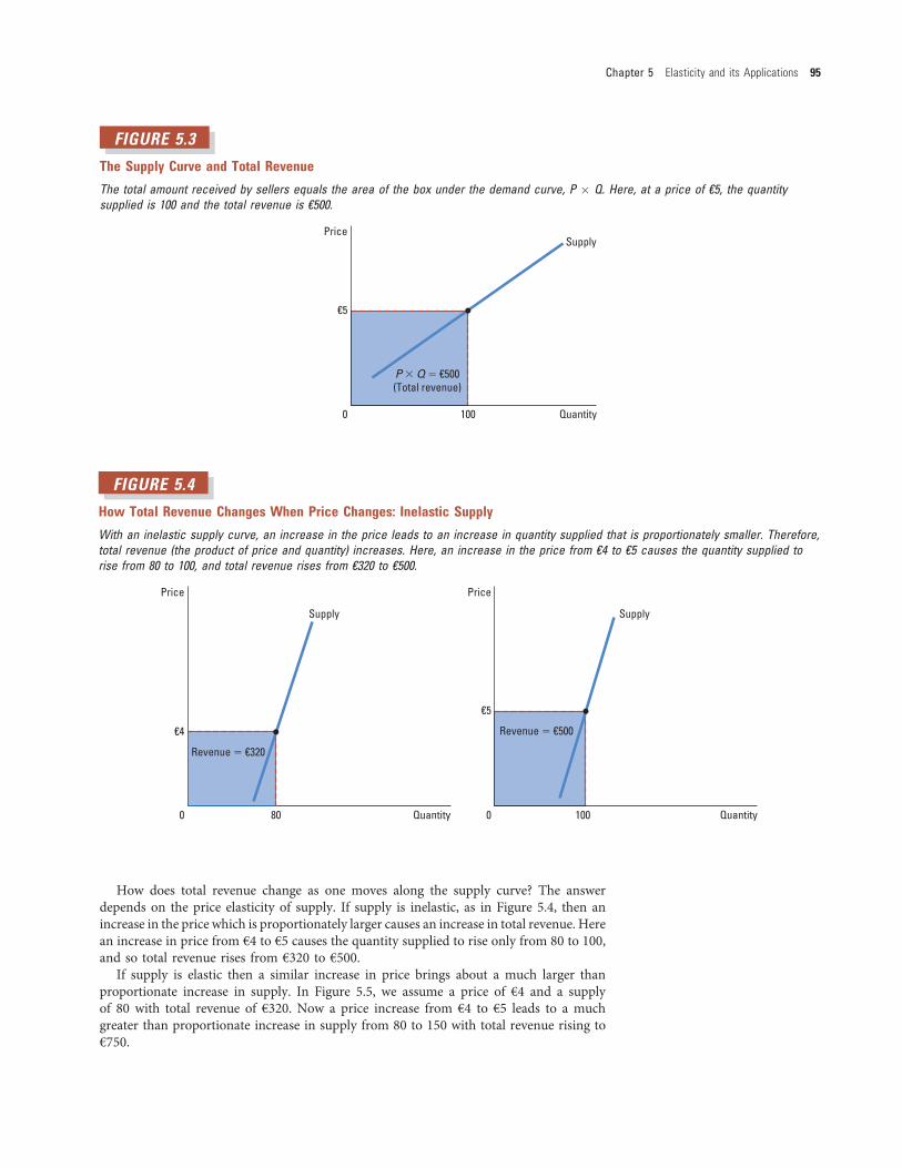
If supply is elastic then a similar increase in price brings about a much larger thanproportionate increase in supply. In Figure 5.5, we assume a price of €4 and a supplyof 80 with total revenue of €320. Now a price increase from €4 to €5 leads to a muchgreater than proportionate increase in supply from 80 to 150 with total revenue rising to€750.

FIGURE 5.3

The Supply Curve and Total Revenue

The total amount received by sellers equals the area of the box under the demand curve, P � Q. Here, at a price of €5, the quantitysupplied is 100 and the total revenue is €500.

Price

€5

0 Quantity100

Supply

P 3 Q 5 €500

(Total revenue)

FIGURE 5.4

How Total Revenue Changes When Price Changes: Inelastic Supply

With an inelastic supply curve, an increase in the price leads to an increase in quantity supplied that is proportionately smaller. Therefore,total revenue (the product of price and quantity) increases. Here, an increase in the price from €4 to €5 causes the quantity supplied torise from 80 to 100, and total revenue rises from €320 to €500.

Price

€4

0 Quantity80

Supply

Revenue 5 €320

Price

€5

0 Quantity100

Supply

Revenue 5 €500


THE PRICE ELASTICITY OF DEMAND

Businesses cannot directly control demand. They can seek to influence demand (and do)by utilizing a variety of strategies and tactics but ultimately the consumer decideswhether to buy a product or not. One important way in which consumer behaviourcan be influenced is through a firm changing the prices of its goods (many firms dohave some control over the price it can charge although as we have seen, in perfectlycompetitive markets this is not the case as the firm is a price taker). An understandingof the price elasticity of demand is important in anticipating the likely effects of changesin price on demand.

The Price Elasticity of Demand and its Determinants

The law of demand states that a fall in the price of a good raises the quantity demanded.The price elasticity of demand measures how much the quantity demanded responds to achange in price. Demand for a good is said to be elastic or price sensitive if the quantitydemanded responds substantially to changes in the price. Demand is said to be inelastic orprice insensitive if the quantity demanded responds only slightly to changes in the price.

The price elasticity of demand for any good measures how willing consumers are tomove away from the good as its price rises. Thus, the elasticity reflects the many economic,social and psychological forces that influence consumer tastes. Based on experience, how-ever, we can state some general rules about what determines the price elasticity of demand.

Availability of Close Substitutes Goods with close substitutes tend to havemore elastic demand because it is easier for consumers to switch from that good toothers. For example, butter and margarine are easily substitutable. A small increase inthe price of butter, assuming the price of margarine is held fixed, causes the quantity ofbutter sold to fall by a relatively large amount. As a general rule, the closer the substitutethe more elastic the good is because it is easier for consumers to switch from one to theother. By contrast, because eggs are a food without a close substitute, the demand foreggs is less elastic than the demand for butter.

FIGURE 5.5

How Total Revenue Changes When Price Changes: Elastic Supply

With an elastic supply curve, an increase in the price leads to an increase in quantity supplied that is proportionately larger. Therefore,total revenue (the product of price and quantity) increases. Here, an increase in the price from €4 to €5 causes the quantity supplied torise from 80 to 150, and total revenue rises from €320 to €750.

Price

€4

0 Quantity80

Supply

Revenue 5 €320

Price

€5

0 Quantity150

Supply

Revenue 5 €750

price elasticity of demand ameasure of how much the quantitydemanded of a good responds to achange in the price of that good,computed as the percentage change inquantity demanded divided by thepercentage change in price


Necessities versus Luxuries Necessities tend to have relatively inelasticdemands, whereas luxuries have relatively elastic demands. People use gas and electricityto heat their homes and cook their food. If the price of gas and electricity rose together,people would not demand dramatically less of them. They might try and be moreenergy-efficient and reduce their demand a little, but they would still need hot foodand warm homes. By contrast, when the price of sailing dinghies rises, the quantity ofsailing dinghies demanded falls substantially. The reason is that most people view hotfood and warm homes as necessities and a sailing dinghy as a luxury. Of course, whethera good is a necessity or a luxury depends not on the intrinsic properties of the good buton the preferences of the buyer. For an avid sailor with little concern over her health,sailing dinghies might be a necessity with inelastic demand and hot food and a warmplace to sleep a luxury with elastic demand.

Definition of the Market The elasticity of demand in any market depends onhow we draw the boundaries of the market. Narrowly defined markets tend to havemore elastic demand than broadly defined markets, because it is easier to find close sub-stitutes for narrowly defined goods. For example, food, a broad category, has a fairlyinelastic demand because there are no good substitutes for food. Ice cream, a narrowercategory, has a more elastic demand because it is easy to substitute other desserts for icecream. Vanilla ice cream, a very narrow category, has a very elastic demand becauseother flavours of ice cream are almost perfect substitutes for vanilla.

Proportion of Income Devoted to the Product Some products have a rela-tively high price and take a larger proportion of income than others. Buying a new suiteof furniture for a lounge, for example, tends to take up a large amount of incomewhereas buying an ice cream might account for only a tiny proportion of income. Ifthe price of a three-piece suite rises by 10 per cent, therefore, this is likely to have agreater effect on demand for this furniture than a similar 10 per cent increase in theprice of an ice cream. The higher the proportion of income devoted to the product thegreater the elasticity is likely to be.

Time Horizon Goods tend to have more elastic demand over longer time horizons.When the price of petrol rises, the quantity of petrol demanded falls only slightly in thefirst few months. Over time, however, people buy more fuel-efficient cars, switch to pub-lic transport and move closer to where they work. Within several years, the quantity ofpetrol demanded falls more substantially. Similarly, if the price of a unit of electricityrises much above an equivalent energy unit of gas, demand may fall only slightly in theshort run because many people already have electric cookers or electric heating appli-ances installed in their homes and cannot easily switch. If the price difference persistsover several years, however, people may find it worth their while to replace their oldelectric heating and cooking appliances with new gas appliances and the demand forelectricity will fall.

Computing the Price Elasticity of Demand

The principles for computing price elasticity of demand are similar to that discussedwhen we looked at price elasticity of supply. The price elasticity of demand is computedas the percentage change in the quantity demanded divided by the percentage change inthe price. That is:

Price elasticity of demand ¼ Percentage change in quantity demandedPercentage change in price


For example, suppose that a 10 per cent increase in the price of a packet of breakfastcereal causes the amount you buy to fall by 20 per cent. Because the quantity demanded ofa good is negatively related to its price, the percentage change in quantity will always havethe opposite sign to the percentage change in price. In this example, the percentage changein price is a positive 10 per cent (reflecting an increase), and the percentage change inquantity demanded is a negative 20 per cent (reflecting a decrease). For this reason, priceelasticities of demand are sometimes reported as negative numbers. In this book we followthe common practice of dropping the minus sign and reporting all price elasticities as pos-itive numbers. (Mathematicians call this the absolute value.) With this convention, a largerprice elasticity implies a greater responsiveness of quantity demanded to price.

Using this convention we calculate the elasticity of demand as:

Price elasticity of demand ¼ 20%10%

¼ 2

In this example, the elasticity is 2, reflecting that the change in the quantity demandedis proportionately twice as large as the change in the price.

Pitfall Prevention We have used the term ‘relatively’ elastic or inelastic at timesthroughout the analysis so far. It is important to remember that elasticity can be anyvalue greater than or equal to 0. We can look at two goods, therefore, both of which areclassed as ‘inelastic’ but where one is more inelastic than the other. If we are compar-ing good X, which has an elasticity of 0.2 and good Y, which has an elasticity of 0.5, thenboth are inelastic but good Y is relatively elastic by comparison. As with so much ofeconomics, careful use of terminology is important in conveying a clear understanding.

Using the Midpoint Method

As with the price elasticity of supply, we use the midpoint method to calculate price elas-ticity of demand for the same reasons. We can express the midpoint method with thefollowing formula for the price elasticity of demand between two points, denoted (Q1,P1) and (Q2, P2):

Price elasticity of demand ¼ ðQ2 � Q1Þ=½ðQ2 þ Q1Þ=2�ðP2 � P1Þ=½ðP2 þ P1Þ=2�

The numerator is the proportionate change in quantity computed using the midpointmethod, and the denominator is the proportionate change in price computed using themidpoint method.

The Variety of Demand Curves

Economists classify demand curves according to their elasticity. Demand is elastic whenthe elasticity is greater than 1, so that quantity changes proportionately more than theprice. Demand is inelastic when the elasticity is less than 1, so that quantity moves pro-portionately less than the price. If the elasticity is exactly 1, so that quantity moves thesame amount proportionately as price, demand is said to have unit elasticity.

Because the price elasticity of demand measures how much quantity demandedresponds to changes in the price, it is closely related to the slope of the demand curve.The following heuristic (rule of thumb) again, assuming we are using comparable scaleson the axes, is a useful guide: the flatter the demand curve that passes through a givenpoint, the greater the price elasticity of demand. The steeper the demand curve thatpasses through a given point, the smaller the price elasticity of demand.

Figure 5.6 shows five cases, each of which uses the same scale on each axis. This is animportant thing to remember because simply looking at a graph and the shape of the


FIGURE 5.6

The Price Elasticity of Demand

The steepness of the demand curve indicates the price elasticity of demand (assuming the scale used on the axes are the same). Notethat all percentage changes are calculated using the midpoint method.

(a) Perfectly inelastic demand: Elasticity equals 0

DemandPrice

€5

4

0 100 90 100Quantity

(b) Inelastic demand: Elasticity is less than 1

Demand

Price

€5

4

0 Quantity

1. A 22%

increase

in price…

2. … leads to an 11% decrease in quantity demanded.2. … leaves the quantity demanded unchanged.

1. An

increase

in price…

80 100

(c) Unit elastic demand: Elasticity equals 1

Demand

Price

€5

4

0 Quantity

1. A 22%

increase

in price…

2. … leads to a 22% decrease in quantity demanded.

(d) Elastic demand: Elasticity is greater than 1

Demand

Price

€5

4

0 10050 Quantity

(e) Perfectly elastic demand: Elasticity equals infinity

Demand

Price

€4

0 Quantity

1. A 22%

increase

in price…

2. … leads to a 67% decrease in quantity demanded.

1. At any price

above €4,quantity

demanded is zero.

2. At exactly €4,

consumers will

buy any quantity.

3. At a price below €4, quantity demanded is infinite.


curve without recognizing the scale can result in incorrect conclusions about elasticity. Inthe extreme case of a zero elasticity shown in panel (a), demand is perfectly inelastic, andthe demand curve is vertical. In this case, regardless of the price, the quantity demandedstays the same. As the elasticity rises, the demand curve gets flatter and flatter, as shownin panels (b), (c) and (d). At the opposite extreme shown in panel (e), demand is per-fectly elastic. This occurs as the price elasticity of demand approaches infinity and thedemand curve becomes horizontal, reflecting the fact that very small changes in theprice lead to huge changes in the quantity demanded.

Total Expenditure, Total Revenue and the Price Elasticity

of Demand

When studying changes in demand in a market, we are interested in the amount paid bybuyers of the good which will in turn represent the total revenue that sellers receive.Total expenditure is given by the total amount bought multiplied by the price paid.We can show total expenditure graphically, as in Figure 5.7. The height of the boxunder the demand curve is P, and the width is Q. The area of this box, P × Q, equalsthe total expenditure in this market. In Figure 5.7, where P ¼ €4 and Q ¼ 100, totalexpenditure is €4 × 100, or €400.

For businesses, having some understanding of the price elasticity of demand is impor-tant in decision making. If a firm is thinking of changing price how will the demand forits product react? The firm knows that there is an inverse relationship between price anddemand but the effect on its revenue will be dependent on the price elasticity of demand.It is entirely possible that a firm could reduce its price and increase total revenue.Equally, a firm could raise price and find its total revenue falling. At first glance thismight sound counter-intuitive but it all depends on the price elasticity of demand for theproduct.

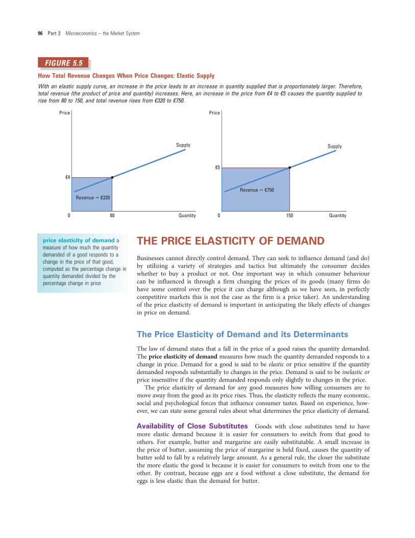
If demand is inelastic, as in Figure 5.8, then an increase in the price causes an increasein total expenditure. Here an increase in price from €1 to €3 causes the quantitydemanded to fall only from 100 to 80, and so total expenditure rises from €100 to€240. An increase in price raises P × Q because the fall in Q is proportionately smallerthan the rise in P.

We obtain the opposite result if demand is elastic: an increase in the price causes adecrease in total expenditure. In Figure 5.9, for instance, when the price rises from €4

FIGURE 5.7

Total Expenditure

The total amount paid by buyers, and received as expenditure by sellers, equals the area of the box under the demand curve, P � Q.Here, at a price of €4, the quantity demanded is 100, and total expenditure is €400.

Price

€4

0 Quantity100

DemandP 3 Q 5 €400

(expenditure)P

Q

total expenditure the amount paidby buyers, computed as the price of thegood times the quantity purchased


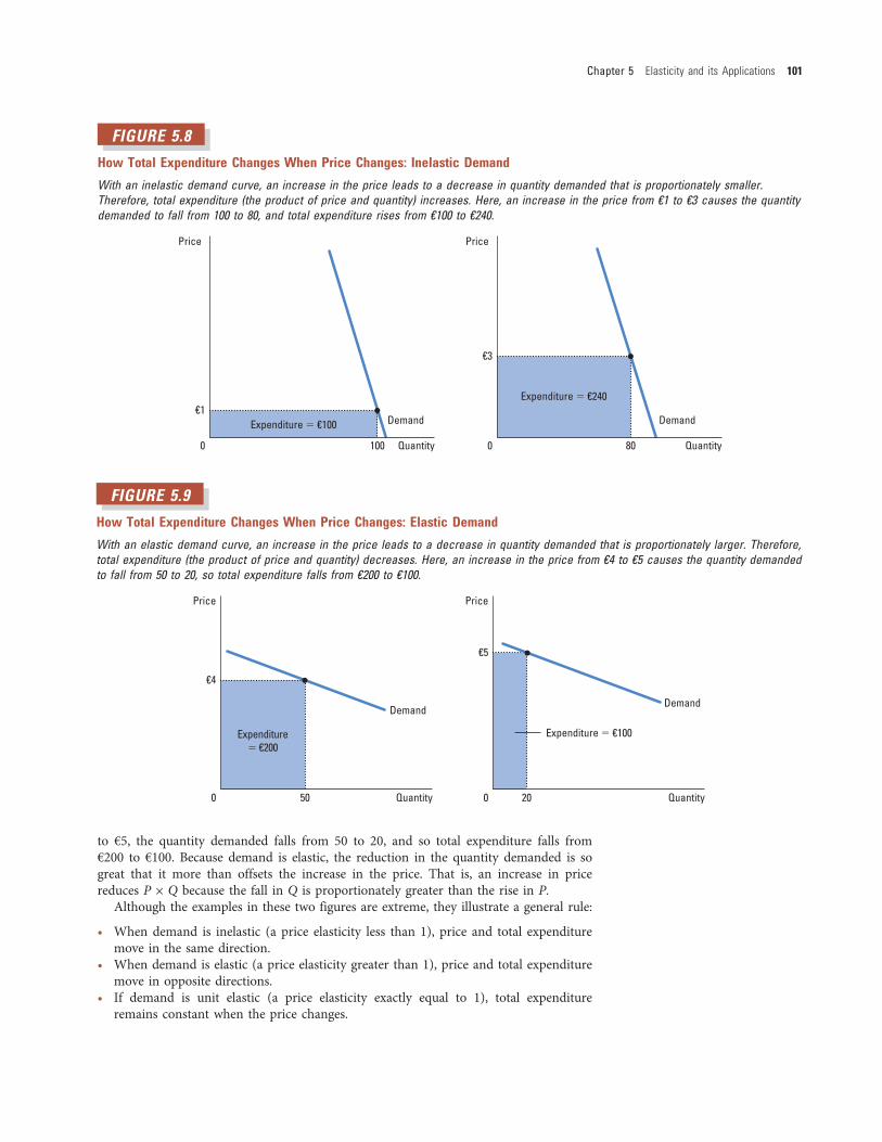
to €5, the quantity demanded falls from 50 to 20, and so total expenditure falls from€200 to €100. Because demand is elastic, the reduction in the quantity demanded is sogreat that it more than offsets the increase in the price. That is, an increase in pricereduces P × Q because the fall in Q is proportionately greater than the rise in P.

Although the examples in these two figures are extreme, they illustrate a general rule:

• When demand is inelastic (a price elasticity less than 1), price and total expendituremove in the same direction.

• When demand is elastic (a price elasticity greater than 1), price and total expendituremove in opposite directions.

• If demand is unit elastic (a price elasticity exactly equal to 1), total expenditureremains constant when the price changes.

FIGURE 5.8

How Total Expenditure Changes When Price Changes: Inelastic Demand

With an inelastic demand curve, an increase in the price leads to a decrease in quantity demanded that is proportionately smaller.Therefore, total expenditure (the product of price and quantity) increases. Here, an increase in the price from €1 to €3 causes the quantitydemanded to fall from 100 to 80, and total expenditure rises from €100 to €240.

Price

Quantity

Expenditure 5 €100 Demand€1

0 100

Price

Quantity

Expenditure 5 €240

Demand

€3

0 80

FIGURE 5.9

How Total Expenditure Changes When Price Changes: Elastic Demand

With an elastic demand curve, an increase in the price leads to a decrease in quantity demanded that is proportionately larger. Therefore,total expenditure (the product of price and quantity) decreases. Here, an increase in the price from €4 to €5 causes the quantity demandedto fall from 50 to 20, so total expenditure falls from €200 to €100.

Price

Quantity

Expenditure

5 €200

Demand

€4

0 50

Price

Quantity

Expenditure 5 €100

Demand

€5

0 20


? what if…a high street clothes retailer is planning its summer sales campaignand wants to cut prices to help it get rid of stock and also increase footfall (thenumber of customers entering its premises) and revenue. It knows of the conceptof price elasticity of demand but how does it set about estimating the price elas-ticity of demand for its products so that it can more accurately set price cutswhich will achieve its aims?

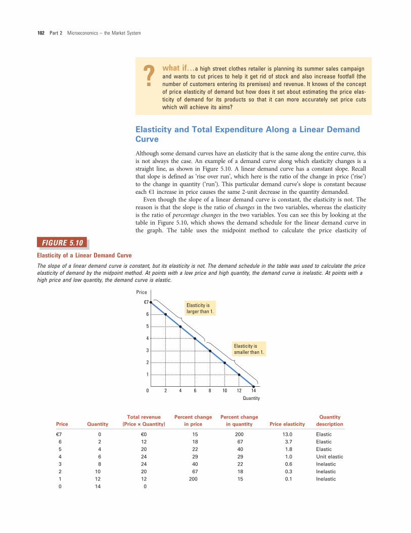
Elasticity and Total Expenditure Along a Linear Demand

Curve

Although some demand curves have an elasticity that is the same along the entire curve, thisis not always the case. An example of a demand curve along which elasticity changes is astraight line, as shown in Figure 5.10. A linear demand curve has a constant slope. Recallthat slope is defined as ‘rise over run’, which here is the ratio of the change in price (‘rise’)to the change in quantity (‘run’). This particular demand curve’s slope is constant becauseeach €1 increase in price causes the same 2-unit decrease in the quantity demanded.

Even though the slope of a linear demand curve is constant, the elasticity is not. Thereason is that the slope is the ratio of changes in the two variables, whereas the elasticityis the ratio of percentage changes in the two variables. You can see this by looking at thetable in Figure 5.10, which shows the demand schedule for the linear demand curve inthe graph. The table uses the midpoint method to calculate the price elasticity of

FIGURE 5.10

Elasticity of a Linear Demand Curve

The slope of a linear demand curve is constant, but its elasticity is not. The demand schedule in the table was used to calculate the priceelasticity of demand by the midpoint method. At points with a low price and high quantity, the demand curve is inelastic. At points with ahigh price and low quantity, the demand curve is elastic.

Price

Quantity

Elasticity is

larger than 1.

Elasticity is

smaller than 1.

€7

6

5

4

3

2

1

0 2 4 6 8 10 12 14

Price Quantity

Total revenue

(Price × Quantity)

Percent change

in price

Percent change

in quantity Price elasticity

Quantity

description

€7 0 €0 15 200 13.0 Elastic

6 2 12 18 67 3.7 Elastic

5 4 20 22 40 1.8 Elastic

4 6 24 29 29 1.0 Unit elastic

3 8 24 40 22 0.6 Inelastic

2 10 20 67 18 0.3 Inelastic

1 12 12 200 15 0.1 Inelastic

0 14 0


demand. At points with a low price and high quantity, the demand curve is inelastic. Atpoints with a high price and low quantity, the demand curve is elastic.

The table also presents total expenditure at each point on the demand curve. Thesenumbers illustrate the relationship between total expenditure and elasticity. When theprice is €1, for instance, demand is inelastic and a price increase to €2 raises total expen-diture. When the price is €5, demand is elastic, and a price increase to €6 reduces totalexpenditure. Between €3 and €4, demand is exactly unit elastic and total expenditure isthe same at these two prices.

In analysing markets, we will use both demand and supply curves on the same dia-gram. We will refer to changes in total revenue when looking at the effects of changesin equilibrium conditions but remember that revenue for sellers represents the sameidentity as expenditure for buyers.

C A S E S T U D YPutting Bums on Seats!

Imagine you are the owner of a coach company running a scheduled bus servicebetween a rural town and surrounding villages. The service runs every two hoursbetween 6 am and 8 pm. The price passengers pay for a return bus journey is astandard fare priced at €3.00. The maximum capacity of each bus is 80 seats.

You have noticed that the number of passengers on the services is falling andyou are considering options to try and increase the demand and fill more seatson each service. You know that price and demand are inversely related and soyou are planning on reducing the price to try and encourage more passengers touse your buses. However, a colleague cautions you against doing this until youhave thought it through in more detail. She suggests that reducing price mightnot be the best option and that you might actually be facing two different demandcurves with different elasticities.

You decide to investigate this idea in more detail. You look at the pattern of bususage throughout the day. Your investigations tell you that the occupancy rate forbuses (the proportion of seats taken up by passengers) on buses between the hoursof 6 am and 8 am is around 95 per cent on average. Between 8 am and 4 pm theoccupancy rate falls considerably to only 30 per cent and climbs again to 90 percent between 4 pm and 6 pm. After 6 pm, the rate falls again to 20 per cent.

The investigation suggests that the demand curve for bus travel in the morningand afternoon rush hour periods is relatively inelastic whereas at other times dur-ing the day the demand curve is more elastic. You reason that rather than justreducing the price as you originally planned, you will charge different prices at dif-ferent times of the day to exploit the different demand curves.

• During the hours of 6 am and 8 am and 4 pm and 6 pm, the price of a returnticket will rise by €1.00 to €4.00.

• Between 8 am and 4 pm the price of a return ticket will fall by 50 per cent to €1.50.• The bus service will stop running after 6.30 pm.

Your colleague advises you to monitor the effect on occupancy rates once thenew prices are introduced. After six months you go back to her with your findings.The increase in the ticket price has resulted in a fall in occupancy rates to 90 percent in the morning and 87 per cent in the afternoon. During the day, the 50 percent cut in the price has raised the occupancy rate from an average of 30 per centto 65 per cent. You are very pleased with the results because although the occu-pancy rates fell in the morning they only fell by a small amount and the increasein price meant that total revenue increased. At other times during the day thereduction in price encouraged more people to use the service and again, theincrease in numbers has led to a rise in revenue.

If the price of a bus ticket washigher would the number of pas-sengers decline?

TADEUSZIBROM/SHUTTERSTOCK


OTHER DEMAND ELASTICITIES

In addition to the price elasticity of demand, economists also use other elasticities todescribe the behaviour of buyers in a market.

The Income Elasticity of Demand

The income elasticity of demand measures how the quantity demanded changes as con-sumer income changes. It is calculated as the percentage change in quantity demandeddivided by the percentage change in income. That is,

Income elasticity of demand ¼ Percentage change in quantity demanded

Percentage change in income

As we discussed in Chapter 4, most goods are normal goods: higher income raisesquantity demanded. Because quantity demanded and income change in the same direc-tion, normal goods have positive income elasticities. A few goods, such as bus rides, areinferior goods: higher income lowers the quantity demanded. Because quantity demandedand income move in opposite directions, inferior goods have negative income elasticities.

Even among normal goods, income elasticities vary substantially in size. Necessities,such as food and clothing, tend to have small income elasticities because consumers,regardless of how low their incomes, choose to buy some of these goods. Luxuries, suchas caviar and diamonds, tend to have high income elasticities because consumers feelthat they can do without these goods altogether if their income is too low.

The Cross-Price Elasticity of Demand

The cross-price elasticity of demand measures how the quantity demanded of one goodchanges as the price of another good changes. It is calculated as the percentage change inquantity demanded of good 1 divided by the percentage change in the price of good 2.That is:

Cross-price elasticity of demand ¼ Percentage change in quantity demanded of good 1Percentage change in the price of good 2

Whether the cross-price elasticity is a positive or negative number depends on whetherthe two goods are substitutes or complements. As we discussed in Chapter 4, substitutesare goods that are typically used in place of one another, such as beef steak and Wienerschnitzel. An increase in the price of beef steak induces people to eat Wiener schnitzelinstead. Because the price of beef steak and the quantity of Wiener schnitzel demandedmove in the same direction, the cross-price elasticity is positive. Conversely, complementsare goods that are typically used together, such as computers and software. In this case, thecross-price elasticity is negative, indicating that an increase in the price of computersreduces the quantity of software demanded. As with price elasticity of demand, cross-price elasticity may increase over time: a change in the price of electricity will have littleeffect on demand for gas in the short run but much stronger effects over several years.

Pitfall Prevention When referring to elasticity it is easy to forget which type ofelasticity you are referring to. It is sensible to ensure that you use the correct terminol-ogy to make sure you are thinking clearly about the analysis and being accurate in yourreferencing to elasticity. If you are analysing the effect of changes in income on demandthen you must specify income elasticity, whereas if you are analyzing changes in priceson supply then you must specify price elasticity of supply and so on.

income elasticity of demand ameasure of how much the quantitydemanded of a good responds to achange in consumers’ income, computedas the percentage change in quantitydemanded divided by the percentagechange in income

cross-price elasticity of

demand a measure of how much thequantity demanded of one goodresponds to a change in the price ofanother good, computed as thepercentage change in quantitydemanded of the first good divided bythe percentage change in the price of thesecond good


Quick Quiz Define the price elasticity of demand. • Explain the rela-

tionship between total expenditure and the price elasticity of demand.

FYI

The Mathematics of Elasticity

We present this section for those whorequire some introduction to the mathsbehind elasticity. For those who do notneed such a technical explanation, thissection can be safely skipped withoutaffecting your overall understanding ofthe concept of elasticity.

Point Elasticity of Demand

Figure 5.10 showed that the value forelasticity can vary at every pointalong a straight line demand curve.Point elasticity of demand allows us tobe able to be more specific about theelasticity at different points. In the for-mula repeated below, the numerator(the top half of the fraction) describes

the change in quantity in relation to thebase quantity and the denominator thechange in price in relation to the baseprice.

ped ¼Q2 �Q1

ððQ2 þQ1Þ=2Þ� �

� 100

P 2 �P 1

ððP 2 þP 1Þ=2Þ� �

� 100

If we cancel out the 100s in theabove equation and rewrite it a littlemore elegantly we get:

ped ¼ΔQQΔPP

Where the ΔQ ¼ Q2 – Q1

Rearranging the above we get:

ped ¼ ΔQQ

� PΔP

There is no set order required tothis equation so it can be re-writtenas:

ped ¼ ΔQΔP

� PQ

The eagle eyed amongst you willnotice that the expression ΔQ/ΔP isthe slope of a linear demand curve.Look at the example in Figure 5.11:

FIGURE 5.11

Price(€)

Quantity

30

25

20

15

10

5

1 2 3 4 5 6

D1 D2


Here we have two demand curves,D1 and D2, given by the equations:

p ¼ 20� 5qand

Q ¼ 5� 0:25p

For demand curve D1, the verticalintercept is 20 and the horizontal interceptis 4 and so the slope of the line D1 is –5.

For demand curve D2, the verticalintercept is 20 and the horizontal inter-cept is 5, the slope of the line D2 is – 4.

To verify this let us take demandcurve D1, if price were 10 then thequantity would be 20 � 5q. Rearranginggives 5q = 20–10, 5q = 10 so q = 20.(Looking at the inverse of this wewould get: 4 � (0.2 � 10) ¼ 2).

Looking at demand curve D2, If pricewere 10, then the quantity would be5 � (0.25 � 10) ¼ 2.5.

Now let us assume that price fallsfrom 10 to 5 in each case. The quantitydemanded for D1 would now be 4 �(0.2 � 5) ¼ 3 and for D2, 5 � (0.25 �5) ¼ 3.75.

Representing this graphically fordemand curve D1, we get the resultshown in Figure 5.12.

The slope of the line as drawn is:

ΔpΔq

¼ �51

¼ �5

The slope is the same at all pointsalong a linear demand curve. The pricewhich we start with prior to a changewill give different ratios at differentpoints on the demand curve. Again,using demand curve D2, the ratio ofP/Q at the initial price of 10 is 10/2 ¼ 5.At a price of 5, the ratio of P/Q given bythe demand curve D2 would be 5/3¼ 1.67.

Going back to our formula:

ped ¼ ΔQΔP

� PQ

The first part of the equation (ΔQ/ΔP)is the slope of the demand curve and thesecond part of the equation P/Q gives usa specific point on the demand curverelating to a particular price and quantitycombination. Multiplying these two termsgives us the price elasticity of demand ata particular point and so is referred to aspoint elasticity of demand.

The price elasticity of demand whenprice changes from 10 to 5 in demandcurve D2 above, would be:

ped ¼ ΔQΔP

� PQ

ped ¼ 15� 10

2ped ¼ 1

If we were looking at a fall in pricefrom 15 to 10 we would get:

ped ¼ ΔQΔP

�PQ

ped ¼ 15� 15

1ped ¼ 3

And if looking at a price fall from 5 to2.5 then we would get:

ped ¼ ΔQΔP

�PQ

ped ¼ 0:55

� 103

ped ¼ 0:33

Calculus

The demand curve is often depicted asa linear curve but there is no reasonwhy it should be linear and can be cur-vilinear. To measure elasticity accu-rately in this case economists usecalculus.

The rules of calculus applied to ademand curve give a far more accuratemeasurement of ped at a particularpoint.

For a linear demand function, theapproximation to the point elasticity

FIGURE 5.12

Price(€)

Quantity

30

25

20

15

10

5

1 2 3 4 5 6

D1 : P � 20 � 5q�Q

�P


at the initial price and quantity is givenby:

ðq2 � q1Þðp2 � p1Þ

� p1q1

which gives exactly the same result asthe point elasticity which is defined interms of calculus and is given by :

dqdp

� pq

Point elasticity defined in terms ofcalculus give a precise answer; allthe other formulae are approximationsof some sort.

The formula looks similar but it mustbe remembered that what we are talkingabout in this instance is an infinitesimallysmall change in quantity following aninfinitesimally small change in priceexpressed by the formula:

ped ¼ dqdp

�PQ

where dq/dp is the derivative of a linearfunction. Given our basic linear equa-tion of the form q ¼ a � bp, the powerfunction rule gives dq/dp as the coeffi-cient of p � (�b).

Take the following demand equation:

q ¼ 60� 3p

To find the price elasticity ofdemand when price¼ 15. First of allwe need to find q.

q ¼ 60� 3pq ¼ 60� 3ð15Þq ¼ 15

We calculate dq/dp as �3.Substitute this into the formula to

get:

ped ¼ �31515

� �ped ¼ �3

Let us frame the demand equationso that p is now being written as afunction of q � this is the equation ofthe inverse demand function.

p ¼ 20� 13q

and we want to find ped when price ¼24 then:

p ¼ 20� 13q

24 ¼ 20� 13q

24� 20 ¼ � 13q

4 ¼ 13q

413

¼ q

12 ¼ q

In this particular case, we mustremember that we are now differentiat-ing p with respect to q so we get:

dp=dq ¼ �12

We cannot simply substitute thisnumber into the formula above, wehave to do a bit of rearranging to takeaccount of how we are viewing therelationship between price and quantityin this instance. So using the inversefunction rule:

dqdp

¼ 1dp=dq

dqdp

¼ � 112

Given that the price is 24 and thequantity is 17.3, the ped is:

ped ¼ dqdp

�PQ

ped ¼ 112

� 2417:3

� �

ped ¼ 0:116

It is useful to remember that given anelasticity figure we can calculate theexpected change in demand as a resultof a change in price. For example, if theped is given as 0.6 then an increase inprice of 5 per cent will result in a fall inquantity demanded of 3 per cent.

By using the inverse of the elasticityequation, for any given value of ped wecan calculate how much of a pricechange is required to bring about adesired change in quantity demanded.

Suppose that a government wanted toreduce the demand for motor vehiclesas part of a policy to reduce congestionand pollution. What sort of pricechange might be required to bringabout a 10 per cent fall in demand?

Assume that the ped for motor vehi-cles is 0.8. The inverse of the basicelasticity formula is:

1ped

¼ % Δp% ΔQ

Substituting our known values intothe formula we get:

10:8

¼ % Dp10

1:25 ¼ % Δp10

%Δp ¼ 12:5

To bring about a reduction indemand of 10 per cent, the price ofmotor vehicles would have to rise by12.5 per cent.

Other Elasticities

Income and cross-elasticity of demandare all treated in exactly the same wayas the analysis of price elasticity ofdemand above. So:

Point income elasticity would be:

yed ¼ dQdY

� YQ

Using calculus:

yed ¼ dqdY

� Yq

For cross-elasticity the formulaswould be:

xed ¼ ΔQa

ΔPb� PbQa

Where Qa is the quantity demandedof one good, a, and Pb is the price of arelated good, b (either a substitute or acomplement).

xed ¼ dqadPb

� PbQa

In Chapter 4 we saw that demandcan be expressed as a multivariatefunction where demand is dependent


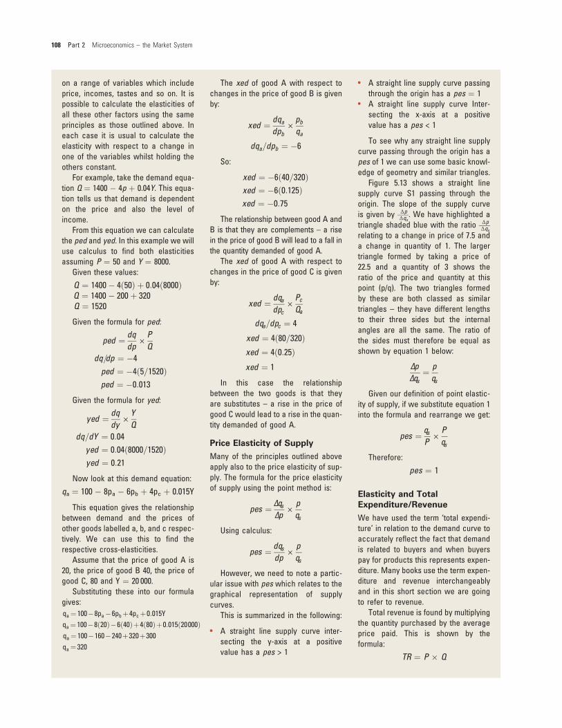
on a range of variables which includeprice, incomes, tastes and so on. It ispossible to calculate the elasticities ofall these other factors using the sameprinciples as those outlined above. Ineach case it is usual to calculate theelasticity with respect to a change inone of the variables whilst holding theothers constant.

For example, take the demand equa-tion Q ¼ 1400 � 4p þ 0.04Y. This equa-tion tells us that demand is dependenton the price and also the level ofincome.

From this equation we can calculatethe ped and yed. In this example we willuse calculus to find both elasticitiesassuming P ¼ 50 and Y ¼ 8000.

Given these values:

Q ¼ 1400� 4ð50Þ þ 0:04ð8000ÞQ ¼ 1400� 200þ 320Q ¼ 1520

Given the formula for ped:

ped ¼ dqdp

×PQ

dq=dp ¼ �4ped ¼ �4ð5=1520Þped ¼ �0:013

Given the formula for yed:

yed ¼ dqdy

×YQ

dq=dY ¼ 0:04yed ¼ 0:04ð8000=1520Þyed ¼ 0:21

Now look at this demand equation:

qa ¼ 100 � 8pa � 6pb þ 4pc þ 0.015Y

This equation gives the relationshipbetween demand and the prices ofother goods labelled a, b, and c respec-tively. We can use this to find therespective cross-elasticities.

Assume that the price of good A is20, the price of good B 40, the price ofgood C, 80 and Y ¼ 20 000.

Substituting these into our formulagives:qa¼ 100�8pa�6pbþ4pcþ0:015Yqa¼ 100�8ð20Þ�6ð40Þþ4ð80Þþ0:015ð20000Þqa¼ 100�160�240þ320þ300qa¼ 320

The xed of good A with respect tochanges in the price of good B is givenby:

xed ¼ dqadpb

×pbqa

dqa=dpb ¼ �6

So:

xed ¼ �6ð40=320Þxed ¼ �6ð0:125Þxed ¼ �0:75

The relationship between good A andB is that they are complements – a risein the price of good B will lead to a fall inthe quantity demanded of good A.

The xed of good A with respect tochanges in the price of good C is givenby:

xed ¼ dqadpc

×PcQa

dqa=dpc ¼ 4

xed ¼ 4ð80=320Þxed ¼ 4ð0:25Þxed ¼ 1

In this case the relationshipbetween the two goods is that theyare substitutes – a rise in the price ofgood C would lead to a rise in the quan-tity demanded of good A.

Price Elasticity of Supply

Many of the principles outlined aboveapply also to the price elasticity of sup-ply. The formula for the price elasticityof supply using the point method is:

pes ¼ ΔqsΔp

×pqs

Using calculus:

pes ¼ dqsdp

×pqs

However, we need to note a partic-ular issue with pes which relates to thegraphical representation of supplycurves.

This is summarized in the following:

• A straight line supply curve inter-secting the y-axis at a positivevalue has a pes > 1

• A straight line supply curve passingthrough the origin has a pes ¼ 1

• A straight line supply curve Inter-secting the x-axis at a positivevalue has a pes < 1

To see why any straight line supplycurve passing through the origin has apes of 1 we can use some basic knowl-edge of geometry and similar triangles.

Figure 5.13 shows a straight linesupply curve S1 passing through theorigin. The slope of the supply curveis given by Δp

Δqs. We have highlighted a

triangle shaded blue with the ratio ΔpΔqs

relating to a change in price of 7.5 anda change in quantity of 1. The largertriangle formed by taking a price of22.5 and a quantity of 3 shows theratio of the price and quantity at thispoint (p/q). The two triangles formedby these are both classed as similartriangles – they have different lengthsto their three sides but the internalangles are all the same. The ratio ofthe sides must therefore be equal asshown by equation 1 below:

ΔpΔqs

¼ pqs

Given our definition of point elastic-ity of supply, if we substitute equation 1into the formula and rearrange we get:

pes ¼ qsP

×Pqs

Therefore:

pes ¼ 1

Elasticity and Total

Expenditure/Revenue

We have used the term ‘total expendi-ture’ in relation to the demand curve toaccurately reflect the fact that demandis related to buyers and when buyerspay for products this represents expen-diture. Many books use the term expen-diture and revenue interchangeablyand in this short section we are goingto refer to revenue.

Total revenue is found by multiplyingthe quantity purchased by the averageprice paid. This is shown by theformula:

TR ¼ P � Q


Total revenue can change if eitherprice or quantity, or both, change there-fore. This can be seen in Figure 5.14where a rise in the price of a goodfrom Po to P1 has resulted in a fall inquantity demanded from Qo to Q1.

We can represent the change inprice as Δp so that the new price is(p þ Δp) and the change in quantity

as Δq so that the new quantity is (q þΔq) so TR can be represented thus:

TR ¼ (p þ Δp) (q þ Δq)

If we multiply out this expression asshown then we get:

TR ¼ pq þ p Δq þ Δpq þ ΔpΔq

In Figure 5.14, this can be seengraphically.

The original TR is found by multi-plying the original price (Po) by theoriginal quantity (Qo) and is shown bythe brown þ blue rectangles.

As a result of the change in pricethere is an additional amount of

FIGURE 5.13

Price(€)

Quantity

30

25

20

15

10

5

1 2 3 4 5 6

�Q

S1

P

�P

Q

FIGURE 5.14

Price(€)

Quantity

Q0Q1

�pq

p�q

D1

�p�qP1

P0

TR 5 (p 1 Δp) (q 1 Δq)


JEOPARDY PROBLEMA business selling plumbing equipment to the trade (i.e. professional plumbersonly) increases the price of copper piping by 4 per cent and reduces the price ofradiators by 5 per cent. A year later they analyse their sales figures and find thatrevenue for copper piping rose in the first three months after the price rise butthen fell dramatically thereafter, while the revenue for sales of radiators also fellthroughout the period.

Explain what might have happened to bring about this situation. Illustrate youranswer with diagrams where appropriate.

APPLICATIONS OF SUPPLY AND DEMANDELASTICITY

Can good news for the computing industry be bad news for computer chip manufac-turers? Why do the prices of ski holidays in Europe rise dramatically over public andschool holidays? At first, these questions might seem to have little in common. Yetboth questions are about markets and all markets are subject to the forces of supplyand demand. Here we apply the versatile tools of supply, demand and elasticity toanswer these seemingly complex questions.

Can Good News for the Computer Industry Be Bad News

for Chip Makers?

Let’s now return to the question posed at the beginning of this chapter: what happens tochip manufacturers and the market for chips when scientists discover a new material formaking chips that is more productive than silicon? Recall from Chapter 4 that we answersuch questions in three steps. First, we examine whether the supply or demand curve

revenue shown by the purple rectan-gle (q Δp). However, this is offset bythe reduction in revenue caused bythe fall in quantity demanded as aresult of the change in price shownby the blue rectangle (p Δq). There isalso an area indicated by the yellowrectangle which is equal to ΔpΔq.This leaves us with a formula forthe change in TR as:

ΔTR ¼ q Δp þ p Δq þ ΔpΔq

Let us substitute some figures intoour formula to see how this works inpractice. Assume the original price ofa product is 15 and the quantity de-manded at this price is 750. Whenprice rises to 20 the quantity de-manded falls to 500.

Using the equation:

TR ¼ pq þ p Δq þ Δpq þ ΔpΔq

TR is now:

TR ¼ 15ð750Þ þ 15ð�250Þ þ 5ð750Þþ 5ð�250ÞTR ¼ 10 000

The change in TR is:

ΔTR ¼ qΔp þ pΔq þ ΔpΔqΔTR ¼ 750ð5Þ þ 15ð�250Þ þ 5ð�250Þ

ΔTR ¼ 3750� 3750� 1250ΔTR ¼ �1250

In this example the effect of thechange in price has been negative onTR. We know from our analysis ofprice elasticity of demand that thismeans the percentage change inquantity demand was greater than

the percentage change in price – inother words, ped must be elastic atthis point (>1). For the change in TR tobe positive, therefore, the ped mustbe <1.

We can express the relationshipbetween the change in TR and pedas an inequality as follows:

ped ¼ ΔQΔP

×PQ> 1

When price increases, revenuedecreases if ped meets this inequali-ty. Equally, for a price increase toresult in a rise in revenue ped mustmeet the inequality below:

ped ¼ ΔQΔP

×PQ<1


shifts. Secondly, we consider which direction the curve shifts. Thirdly, we use the supplyand demand diagram to see how the market equilibrium changes.

This is a situation that is facing chip manufacturers. Scientists are investigating newmaterials to make computer chips. Such a material may allow the manufacturers to beable to work on building processing power at ever smaller concentrations and increase com-puting power considerably. In this case, the discovery of the new material affects the supplycurve. Because the material increases the amount of computing power that can be producedon each chip, manufacturers are now willing to supply more chips at any given price. Inother words, the supply curve for computing power shifts to the right. The demand curveremains the same because consumers’ desire to buy chips at any given price is not affectedby the introduction of the new material. Figure 5.15 shows an example of such a change.When the supply curve shifts from S1 to S2, the quantity of chips sold increases from 100to 110, and the price of chips falls from €10 per gigabyte to €4 per gigabyte.

But does this discovery make chip manufacturers better off? As a first stab at answeringthis question, consider what happens to the total revenue received by chip manufacturers;total revenue is P × Q, the price of each chip times the quantity sold. The discovery affectsmanufacturers in two conflicting ways. The new material allows manufacturers to producemore chips with greater computing power (Q rises), but now each chip sells for less (P falls).

Whether total revenue rises or falls depends on the elasticity of demand. We canassume that the demand for chips is inelastic; in producing a computer, chips representa relatively small proportion of the total cost but they also have few good substitutes.When the demand curve is inelastic, as it is in Figure 5.15, a decrease in price causestotal revenue to fall. You can see this in the figure: the price of chips falls substantially,whereas the quantity of chips sold rises only slightly. Total revenue falls from €1000 to€440. Thus, the discovery of the new material lowers the total revenue that chip manu-facturers receive for the sale of their products.

If manufacturers are made worse off by the discovery of this new material, why dothey adopt it? The answer to this question goes to the heart of how competitive marketswork. If each chip manufacturer is a small part of the market for chips, he or she takes

FIGURE 5.15

An Increase in Supply in the Market for Computer Chips

When an advance in chip technology increases the supply of chips from S1 to S2, the price of chips falls. Because the demand for chips isinelastic, the increase in the quantity sold from 100 to 110 is proportionately smaller than the decrease in the price from €10 to €4. As aresult, manufacturers’ total revenue falls from €1000 (€10 � 100) to €440 (€4 � 110).

Price of

chips

Quantity of

chips

2. … leads

to a large fall

in price…

€10

4

0 100 110

1. When demand is inelastic,

an increase in supply…

Demand

3. … and a proportionately smaller

increase in quantity sold. As a result,

revenue falls from €300 to €220.

S1 S2


the price of chips as given. For any given price of chips, it is better to use the new mate-rial in order to produce and sell more chips. Yet when all manufacturers do this, thesupply of chips rises, the price falls and manufacturers are worse off.

Although this example is only hypothetical, in fact a new material for making com-puter chips is being investigated. The material is called hafnium and is used in thenuclear industry. In recent years the manufacture of computer chips has changed dra-matically. In the early 1990s, prices per megabyte of DRAM (dynamic random accessmemory) stood at around $55 but fell to under $1 by the early part of the new century.Manufacturers who were first involved in chip manufacture made high profits but asnew firms joined the industry, supply increased and as the technology also spread, sup-ply rose and prices fell. The fall in prices led to a number of firms struggling to stay inbusiness. We assumed above that computer chip manufacturers were price takers but inreality the computer chip market is not perfectly competitive. However, the fact that somany smaller manufacturers struggled to survive as chip technology expanded at such arapid rate from the early 1990s shows that even markets dominated now by a relativelysmall number of firms exhibit many of the features we have described so far.

When analysing the effects of technology, it is important to keep in mind that what isbad for manufacturers is not necessarily bad for society as a whole. Improvement incomputing power technology can be bad for manufacturers who find it difficult to sur-vive unless they are very large, but it represents good news for consumers of this com-puting power (ultimately the users of PCs, laptops, smartphones and so on) who pay lessfor computing.

Why Do Prices of Ski Holidays Differ so Much at Different

Times of the Season?

Ski holidays in Europe are becoming ever more popular. There were over one millionpeople from the UK who were part of the snowsports travel market in 20112. For anincreasing number of people the pleasure of a holiday on the slopes is a part of the win-ter but people also face considerable changes in the prices that they have to pay for theirholiday. For example, a quick check of a ski company website for the 2011–2012 seasonrevealed the prices shown in Table 5.1 for seven-night ski trips per person to Austrialeaving from London.

There is a considerable variation in the prices that holidaymakers have to pay – £490being the greatest difference. Prices are particularly high leaving on 29 December and12 February – why? The reason is that at this time of the season the demand for ski

TABLE 5.1

Prices for 7-night Ski Holidays in Austria, From London

Departure date Price per person (£)

29 December 2011 262

8 January 2012 228

15 January 2012 194

22 January 2012 194

29 January 2012 194

5 February 2012 251

12 February 2012 684



2http://www.skiclub.co.uk/assets/files/documents/snowsportsanalysis2011.pdf


holidays increases dramatically because they coincide with annual holiday periods; 29December is part of the Christmas/New Year holidays and when schoolchildren arealso on holiday; 12 February is also a major school holiday for many UK children.

The supply of ski holidays does have a limit – there will be a finite number of accom-modation places and passes for ski-lifts and so the elasticity of supply is relatively inelas-tic (see Panel b, Figure 5.16). It is difficult for tour operators to increase supply ofaccommodation or ski-passes easily in the short run in the face of rising demand atthese times. The result is that the increase in demand for ski holidays at these peaktimes results in prices rising significantly to choke off the excess demand. If holiday-makers are able to be flexible about when they take their holidays then they will be ableto benefit from lower prices for the same holiday. Away from these peak periods thedemand for ski holidays is lower and so tour operators have spare capacity – the supplycurve out of peak times is more elastic in the short run. If there was a sudden increase indemand in mid-January, for example, then tour operators would have the capacity toaccommodate that demand so prices would not rise as much as when that capacity isstrictly limited.

Cases for which supply is very inelastic in the short run but more elastic in the longrun may see different prices exist in the market. Air and rail travel and the use of elec-tricity may all be examples where prices differ markedly at peak times compared withoff-peak times because of supply constraints and the ability of firms to be able to dis-criminate between customers at these times.

Quick Quiz How might a drought that destroys half of all farm crops be

good for farmers? If such a drought is good for farmers, why don’t farmers

destroy their own crops in the absence of a drought?

FIGURE 5.16

The Supply of Ski Holidays in Europe

Panel (a) shows the market for ski holidays in off-peak times. The supply curve S1 is relatively elastic in the short run. An increase indemand from D1 to D2 at this time leads to a relatively small increase in price because the increase can be accommodated by releasingsome of the spare capacity that tour operators have. Panel (b) shows the market during peak times. The supply of holidays shown by thecurve S1 is relatively inelastic in the short run. If demand now increases from D1 to D2 the result will be a sharp rise in price.

(a) Off peak (b) Peak times

Quantity of ski holidays

bought and sold (000s)

228

194

0 250 340

Price of

ski holidays

per person (£)

S1

D1 D2

S1

684

251

1300 1350

Quantity of ski holidays

bought and sold (000s)

Price of

ski holidays

per person (£)

D1D2


FYI

Estimates of Elasticities

We have discussed the concept ofelasticity in general terms but there isempirical evidence on elasticity of pro-ducts in the real world. We present

some examples of estimates of priceelasticity of supply and demand for arange of products in Table 5.2. It mustbe remembered that the following are

estimates and you may find other esti-mates where the elasticities differ fromthose given here.

TABLE 5.2

Estimates of Price Elasticity of Supply

Good PES estimate

Public transport in Sweden 0.44 to 0.64

Labour in South Africa 0.35 to 1.75

Beef• Zimbabwe

• Brazil

• Argentina

2.0

0.11 to 0.56

0.67 to 0.96

Corn (short run in US) 0.96

Housing, long run in selected US cities Dallas: 38.6

San Francisco:

2.4

New Orleans: 0.9

St. Louis: 8.1

Uranium 2.3 to 3.3

Recycled aluminium 0.5

Oysters 1.64 to 2.00

Retail store space 3.2

Natural gas (short run) 0.5

Source: http://signsofchaos.blogspot.com/2005/11/price-elasticity-of-sup-

ply-and-web.html

Estimates of Price Elasticity of Demand

Good PED estimate

Tobacco 0.4

Milk 0.3

Wine 0.6

Shoes 0.7

Cars 1.9

Particular brand of car 4.0

Movies 0.9

Entertainment 1.4

Furniture 3.04

Fuel 0.4

Bread 0.25


IN THE NEWS

Price Elasticity of Demand in the Hotel IndustryThere are few industries where the concept of elasticity is not relevant but it is just one factor inbusiness decision making. The hotel industry is not a perfectly competitive market but hotels doface considerable competition from rivals. Hotel owners have some influence over the price theycharge for the service they provide and a consideration of the concept of elasticity is important indecision making. This article refers to some of these other factors as well as emphasizing theimportance of factors affecting price elasticity of demand.

The Making of Mafraq

The National Investor’s (TNI) purchaseof the 15-year-old Mafraq Hotel in AbuDhabi in April 2007 was the company’sfirst direct hospitality acquisition. But,with the firm’s founding principlebeing to incubate UAE-based busi-nesses aligned to the Abu Dhabi 2030vision – in which tourism plays a pivotalrole – it was a ‘natural choice’, recallsTNI vice president, real estate agent,Robert Rowell.

Fast forward four and half years andthe company has since invested US $50million in extending and upgrading thehotel. Far more than a face lift, the fullrenovation has resulted in a sleek, mod-ern hotel with 250 rooms instead of 120,its dated former self a mere shadow. Allachieved while the hotel remainedopen, not quite on time but most defi-nitely on budget, reveals Rowell. Manyowners are forced to invest such sumsto bring their properties up to the brandstandards of their appointed operators,but this is where Mafraq has a point ofdifference – TNI decided to manage itin-house and keep the original name.

The general manager, GhassanFares, previously a GM at HabtoorHotels, joined Mafraq in November2007 to deliver TNI’s vision. And forFares, the freedom bestowed on himby the company has played a majorrole in the hotel’s ongoing success.Rowell and Fares appear to work sideby side, finishing each other’s sentencesand radiating a distinct sense of pride inwhat they have achieved at Mafraq.

The project marks TNI out as a boldnew hospitality investor, avoiding thebrand bandwagon and going it alone –

controversial perhaps at a time whenAbu Dhabi is welcoming numerousglobal names. It highlights the issue ofwhether brands are always best anddemonstrates that there are indeedother options, so Hotelier paid Mafraqa visit… and was pleasantly impressedwith this secluded Abu Dhabi hotel. Here,Rowell and Fares explain the philosophybehind their owner-operator partnershipand their ‘bullish’ approach to 2012.

What was the Mafraq Hotel like

when you acquired it?

Rowell: In 2007 we had a four-star hotelthat was around 15 years old. It was inneed of a refurbishment. The hotel had120 rooms with one all-day-dining facil-ity. We saw the occupancy levels in theexisting hotel and the local demand andrealized there was a clear investmentcase to expand it from 120 rooms to 250rooms and to fortify the product offeringby including a speciality restaurant anda ballroom, within the four-star target.

When will you see return on

investment on your acquisition?

Rowell: I think a rule of thumb for model-ling investment returns on a hotel wouldbe approximately, or under, 10 years interms of being able to return the initialamount invested, and I think we’ll com-fortably be within that return time frame.The hotel has already exceeded ourexpectations in terms of the room rateswhich increased rapidly; certainly for

the first couple of years after 2007 theroom rates were increasing but theoccupancy wasn’t decreasing so for usthere was a low price elasticity ofdemand, a low correlation of pricesgoing up and occupancy going down,so that gave us even more encourage-ment that the asset was a good one andwould be good for a long time.

Now the property has its

new-look, what will be your

approach to driving rates

and occupancy?

Fares: We’re in line with the market fora four-star property, in the AED 500s.During the Abu Dhabi Grand Prix wedid very well.

We are regaining all of our corpo-rate clients because during construc-tion some of them moved out. But wenever lost touch with them, we keptvisiting them, making sales calls atleast weekly, we invited them to differ-ent areas, sometimes took them to adifferent hotel because we didn’t havefacilities to serve clients here. Westayed proactive on that part of it.They don’t believe this is really theproperty they were staying in before!

I’m not worried at all in keeping thisproperty running and getting profit outof it. We did it in the tough days andwhen the property was really deterio-rated; it wasn’t that great in terms ofstanding, now it’s brand new with alot of facilities. It’s a product that cancompete with other properties,whereas earlier it was challenging forme to compete with other properties.


We can talk with more confidencenow and we can convince clients look-ing for meetings, incentives, confer-ences and exhibitions (MICE) businessthat we are the place for them. The AbuDhabi Tourism Authority (ADTA) hasdone well on promoting Abu Dhabi asa MICE sector; earlier we had 3–5 percent of business in MICE, now we’reexpecting to have 10 per cent.

What and where is your

competition?

Fares: The Yas Island hotels are com-peting because they are dropping their

rates tremendously. There are furn-ished hotel apartments coming up andthat’s also a challenge because lookingat the business around us it’s long-term,when you have a guest that stays withyou for a minimum stay of 10 nights,many look for cooking facilities; that’sa challenge there for us.

Rowell: It’s those other segmentsthat we’re not catering for, trying tocompete with our segment, possibly aserviced apartment coming in to thearea and competing for the long stayingguest; or it’s the five stars trying to com-pete on rate, which hurts them in thelong run, just to take those clients. Gen-erally it’s the closer hotels to us but it’s apretty captive market as there’s a limitednumber around us.

You’ve now celebrated the

official relaunch on November

18, what next?

Rowell: We’re very much focused onpushing forward into 2012, we’re verybullish on the short, medium and longterm of the hotel and the area around ithere so we’re focusing on operationsnow. We’ve just come out of develop-ment, so now it’s 100 per cent focus on

getting the operating efficiency back towhere it was and employing staff,retaining the right staff and eventuallymaking profit. We’re bullish over thenext 12 months despite the upcomingsupply.

Questions1. Why might TNI have wanted to keep

the Mafraq Hotel open during reno-vation and refurbishment?

2. Why might hotel chains establishbrands? Use examples to illustrateyour answer.

3. What do you think is meant by thephrase ‘return on investment’?

4. What factors might influence theprice elasticity of supply anddemand for hotel accommodationsuch as that at Mafraq?

5. How might a knowledge of the priceelasticity of demand for Mafraqbeing ‘low’ be useful to its ownersin making pricing decisions?

Source: adapted from http://www.hoteliermiddleeast.com/13087-the-making-of-mafraq/1/ 11 December 2011, accessed29 December 2011.

SUMMARY

• The price elasticity of supply measures how much the quan-tity supplied responds to changes in the price. This elasticityoften depends on the time horizon under consideration. Inmost markets, supply is more elastic in the long run than inthe short run.

• The price elasticity of supply is calculated as the percentagechange in quantity supplied divided by the percentagechange in price. If the elasticity is less than 1, so that quan-tity supplied moves proportionately less than the price, sup-ply is said to be inelastic. If the elasticity is greater than 1, sothat quantity supplied moves proportionately more than theprice, supply is said to be elastic.

• The price elasticity of demand measures how much thequantity demanded responds to changes in the price.Demand tends to be more elastic if close substitutes are

available, if the good is a luxury rather than a necessity, ifthe market is narrowly defined or if buyers have substantialtime to react to a price change.

• The price elasticity of demand is calculated as the percent-age change in quantity demanded divided by the percentagechange in price. If the elasticity is less than 1, so that quan-tity demanded moves proportionately less than the price,demand is said to be inelastic. If the elasticity is greaterthan 1, so that quantity demanded moves proportionatelymore than the price, demand is said to be elastic.

• Total revenue, the total amount received by sellers for agood, equals the price of the good times the quantity sold.For inelastic demand curves, total revenue rises as pricerises. For elastic demand curves, total revenue falls as pricerises.

©MAFRAQ

HOTELS


• The income elasticity of demand measures how much thequantity demanded responds to changes in consumers’income. The cross-price elasticity of demand measureshow much the quantity demanded of one good responds tochanges in the price of another good.

• The tools of supply and demand can be applied in many dif-ferent kinds of markets. This chapter uses them to analysethe market for computer chips and the market for skiholidays.

KEY CONCEPTS

elasticity, p. 88price elasticity of supply, p. 88total revenue, p. 94

price elasticity of demand, p. 96total expenditure, p. 100income elasticity of demand, p. 104

cross-price elasticity of demand, p. 104

QUEST IONS FOR REVIEW1. How is the price elasticity of supply calculated? Explain

what this measures.

2. Is the price elasticity of supply usually larger in the short runor in the long run? Why?

3. What are the main factors that affect the price elasticity ofsupply? Think of some examples to use to illustrate thefactors you cover.

4. Define the price elasticity of demand and the income elas-ticity of demand.

5. List and explain some of the determinants of the priceelasticity of demand. Think of some examples to use toillustrate the factors you cover.

6. If the elasticity is greater than 1, is demand elastic orinelastic? If the elasticity equals 0, is demand perfectlyelastic or perfectly inelastic?

7. On a supply and demand diagram, show equilibrium price,equilibrium quantity and the total revenue received byproducers.

8. If demand is elastic, how will an increase in price changetotal revenue? Explain.

9. What do we call a good whose income elasticity is lessthan 0?

10. In the 2000s, house prices in many parts of the world rosesignificantly. Outline some of the factors that will affect theelasticity of supply and demand for houses in the short runand the long run.

PROBLEMS AND APPL ICAT IONS1. Seafront properties along the promenade at Brighton on the

south coast of England have an inelastic supply, and carshave an elastic supply. Suppose that a rise in populationdoubles the demand for both products (that is, the quantitydemanded at each price is twice what it was).a. What happens to the equilibrium price and quantity in

each market?b. Which product experiences a larger change in price?c. Which product experiences a larger change in quantity?d. What happens to total consumer spending on each

product?

2. Because better weather makes farmland more productive,farmland in regions with good weather conditions is moreexpensive than farmland in regions with bad weather con-ditions. Over time, however, as advances in technology havemade all farmland more productive, the price of farmland(adjusted for overall inflation) has fallen. Use the concept ofelasticity to explain why productivity and farmland pricesare positively related across space but negatively relatedover time.

3. For each of the following pairs of goods, which good wouldyou expect to have a more price elastic demand and why?

a. Required textbooks or mystery novels.b. Beethoven recordings or classical music recordings in

general.c. Heating oil during the next six months or heating oil

during the next five years.d. Lemonade or water.

4. Suppose that business travellers and holidaymakers havethe following demand for airline tickets from Birmingham toNaples:

Price (€)

Quantity demanded

(business travellers)

Quantity demanded

(holidaymakers)

150 2100 1000

200 2000 800

250 1900 600

300 1800 400

a. As the price of tickets rises from €200 to €250, what isthe price elasticity of demand for (i) business travellersand (ii) holidaymakers? (Use the midpoint method in yourcalculations.)

b. Why might holidaymakers have a different elasticity frombusiness travellers?


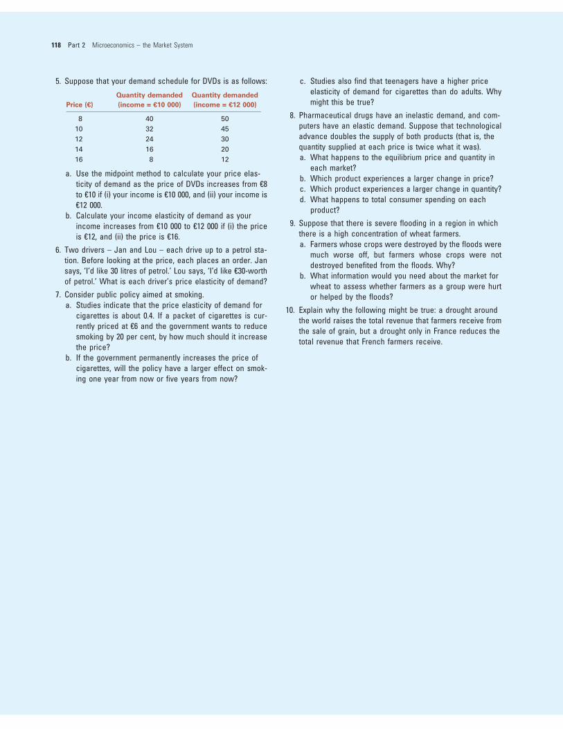
5. Suppose that your demand schedule for DVDs is as follows:

Price (€)

Quantity demanded

(income = €10 000)

Quantity demanded

(income = €12 000)

8 40 50

10 32 45

12 24 30

14 16 20

16 8 12

a. Use the midpoint method to calculate your price elas-ticity of demand as the price of DVDs increases from €8to €10 if (i) your income is €10 000, and (ii) your income is€12 000.

b. Calculate your income elasticity of demand as yourincome increases from €10 000 to €12 000 if (i) the priceis €12, and (ii) the price is €16.

6. Two drivers – Jan and Lou – each drive up to a petrol sta-tion. Before looking at the price, each places an order. Jansays, ‘I’d like 30 litres of petrol.’ Lou says, ‘I’d like €30-worthof petrol.’ What is each driver’s price elasticity of demand?

7. Consider public policy aimed at smoking.a. Studies indicate that the price elasticity of demand for

cigarettes is about 0.4. If a packet of cigarettes is cur-rently priced at €6 and the government wants to reducesmoking by 20 per cent, by how much should it increasethe price?

b. If the government permanently increases the price ofcigarettes, will the policy have a larger effect on smok-ing one year from now or five years from now?

c. Studies also find that teenagers have a higher priceelasticity of demand for cigarettes than do adults. Whymight this be true?

8. Pharmaceutical drugs have an inelastic demand, and com-puters have an elastic demand. Suppose that technologicaladvance doubles the supply of both products (that is, thequantity supplied at each price is twice what it was).a. What happens to the equilibrium price and quantity in

each market?b. Which product experiences a larger change in price?c. Which product experiences a larger change in quantity?d. What happens to total consumer spending on each

product?

9. Suppose that there is severe flooding in a region in whichthere is a high concentration of wheat farmers.a. Farmers whose crops were destroyed by the floods were

much worse off, but farmers whose crops were notdestroyed benefited from the floods. Why?

b. What information would you need about the market forwheat to assess whether farmers as a group were hurtor helped by the floods?

10. Explain why the following might be true: a drought aroundthe world raises the total revenue that farmers receive fromthe sale of grain, but a drought only in France reduces thetotal revenue that French farmers receive.


5 ELASTICITYANDITS APPLICATIONS - … · 5 ELASTICITYANDITS APPLICATIONS ... Learn the meaning of the concept of elasticity ... Distinguish between the price elasticity of demand

Documents