1 Paper 491-2013 DICHOTOMIZED_D: A SAS ® Macro for Computing Effect Sizes for Artificially Dichotomized Variables Patrice Rasmussen, Isaac Li, Patricia Rodriguez de Gil, Jeanine Romano, Rheta E. Lanehart, Aarti P. Bellara, George MacDonald, Harold Holmes, Yi-Hsin Chen, Jeffrey D. Kromrey, University of South Florida, Tampa, Fl. ABSTRACT Measures of effect size are recommended to communicate information on the strength of relationships between variables, providing information to supplement the reject / fail-to-reject decision obtained in statistical hypothesis testing. With artificially dichotomized response variables, seven methods have been proposed to estimate the standardized mean difference effect size that would have been realized before dichotomization. This paper provides a SAS macro for computing these seven effect size estimates by utilizing data from PROC FREQ output data sets. The paper provides the macro programming language, as well as results from an executed example of the macro. Keywords: EFFECT SIZES, DICHOTOMIZED VARIABLES, BASE SAS, SAS/STAT INTRODUCTION The topic of effect sizes can be a controversial issue for many journal editors, as well as for researchers. For instance, Pedhazur and Pedhazur-Schmelking (1991) argued that Cohen’s (1988) convention of small, medium, and large effect sizes distorted the distinction between the magnitude of an effect and its substantive importance, i.e., researchers relegating “small” effects as less important or considering “large” effects as important. Also, the use and interpretation of a specific effect size across studies can be problematic due to the variability of research design factors, the last edition of the Publication Manual of the American Psychological Association (6 th edition; 2010) as well as the 1999 report by Wilkinson and the APA Task Force on Statistical Inference have made clear the imperative for reporting effect sizes to supplement statistical hypothesis testing and ensure “accuracy of scientific knowledge” (p. 11). Effect sizes provide useful indices of the magnitudes of treatment effects in individual studies as well as representing the primary statistics that are used in synthetizing research or meta-analysis. Cohen (1977) defined effect size (ES) as “the degree to which the phenomenon is present in the population” (pp. 9 - 10), or “the degree to which the H0 is believed to be false” (1992; p. 156). Each statistical test has its own ES index, which is scale free and continuous; however, to convey meaning of any ES index, it is necessary to have an idea of its scale, for which he proposed the small, medium, and large ES conventions. One ES index of mean differences is d. That is, for studies comparing two groups on a continuous outcome variable, the standardized mean difference (also referred to as Cohen’s d) is the most common index of effect size. In a population, this ES is obtained as E C where E and C are the means of the experimental and control populations, respectively, and is the common population standard deviation. A sample estimate of this effect size (d) is obtained by substituting sample statistics for each of these parameters. The sampling variance of this estimate is given by 2 2 2 E C d E C E C n n d S nn n n . In medical and social science research, continuous outcome variables are often dichotomized using a cut score to delineate the two dichotomous values. For example, measures of blood pressure or depression may be obtained on a continuous scale, but are subsequently dichotomized to classify patients as hypertensive or clinically depressed. Similarly, educational achievement measures may be obtained as a continuous variable (number of test items correct or scale score on a standardized achievement test) and subsequently dichotomized into pass / fail. With such dichotomization, the standardized mean difference can no longer be directly estimated from sample data. A variety of statistics have been proposed to provide estimates of the standardized mean difference that would have Statistics and Data Analysis SAS Global Forum 2013

Welcome message from author
This document is posted to help you gain knowledge. Please leave a comment to let me know what you think about it! Share it to your friends and learn new things together.
Transcript

1
Paper 491-2013
DICHOTOMIZED_D: A SAS® Macro for Computing Effect Sizes for Artificially Dichotomized Variables
Patrice Rasmussen, Isaac Li, Patricia Rodriguez de Gil, Jeanine Romano,
Rheta E. Lanehart, Aarti P. Bellara, George MacDonald, Harold Holmes,
Yi-Hsin Chen, Jeffrey D. Kromrey,
University of South Florida, Tampa, Fl.
ABSTRACT
Measures of effect size are recommended to communicate information on the strength of relationships between variables, providing information to supplement the reject / fail-to-reject decision obtained in statistical hypothesis testing. With artificially dichotomized response variables, seven methods have been proposed to estimate the standardized mean difference effect size that would have been realized before dichotomization. This paper provides a SAS
macro for computing these seven effect size estimates by utilizing data from PROC FREQ output data sets.
The paper provides the macro programming language, as well as results from an executed example of the macro.
Keywords: EFFECT SIZES, DICHOTOMIZED VARIABLES, BASE SAS, SAS/STAT
INTRODUCTION
The topic of effect sizes can be a controversial issue for many journal editors, as well as for researchers. For instance, Pedhazur and Pedhazur-Schmelking (1991) argued that Cohen’s (1988) convention of small, medium, and large effect sizes distorted the distinction between the magnitude of an effect and its substantive importance, i.e., researchers relegating “small” effects as less important or considering “large” effects as important. Also, the use and interpretation of a specific effect size across studies can be problematic due to the variability of research design factors, the last edition of the Publication Manual of the American Psychological Association (6
th edition; 2010) as well
as the 1999 report by Wilkinson and the APA Task Force on Statistical Inference have made clear the imperative for reporting effect sizes to supplement statistical hypothesis testing and ensure “accuracy of scientific knowledge” (p. 11). Effect sizes provide useful indices of the magnitudes of treatment effects in individual studies as well as representing the primary statistics that are used in synthetizing research or meta-analysis.
Cohen (1977) defined effect size (ES) as “the degree to which the phenomenon is present in the population” (pp. 9-10), or “the degree to which the H0 is believed to be false” (1992; p. 156). Each statistical test has its own ES index,
which is scale free and continuous; however, to convey meaning of any ES index, it is necessary to have an idea of its scale, for which he proposed the small, medium, and large ES conventions.
One ES index of mean differences is d. That is, for studies comparing two groups on a continuous outcome variable, the standardized mean difference (also referred to as Cohen’s d) is the most common index of effect size. In a
population, this ES is obtained as
E C
where E and
C are the means of the experimental and control populations, respectively, and is the common
population standard deviation.
A sample estimate of this effect size (d) is obtained by substituting sample statistics for each of these parameters. The sampling variance of this estimate is given by
22
2
E Cd
E C E C
n n dS
n n n n
.
In medical and social science research, continuous outcome variables are often dichotomized using a cut score to delineate the two dichotomous values. For example, measures of blood pressure or depression may be obtained on a continuous scale, but are subsequently dichotomized to classify patients as hypertensive or clinically depressed. Similarly, educational achievement measures may be obtained as a continuous variable (number of test items correct or scale score on a standardized achievement test) and subsequently dichotomized into pass / fail. With such dichotomization, the standardized mean difference can no longer be directly estimated from sample data. A variety of statistics have been proposed to provide estimates of the standardized mean difference that would have
Statistics and Data AnalysisSAS Global Forum 2013

2
been obtained if the data had not been dichotomized. These effect sizes have been compared in Monte Carlo studies reported by Sanchez-Meca, Marín-Martínez and Chacón-Moscoso, (2003), and by Kromrey and Bell (2012).
ALTERNATIVE METHODS FOR COMPUTING DICHOTIZMIZED EFFECT SIZES
The standardized proportion difference (dp; Johnson, 1989) is a direct analogy to the standardized mean difference
E Cp
P Pd
S
where PE and PC are the sample success (or failure) proportions of the experimental and control groups. The pooled
standard deviation is obtained as
( 1) (1 ) ( 1) (1 )
2
E E E C C C
E C
n P P n P PS
n n
.
The sampling variance of this statistic is obtained as
2
2
2p
pE Cd
E C E C
dn nS
n n n n
.
The phi coefficient ( ) is commonly used as a measure of association for 2 X 2 tables. This index can be transformed to the scale of the standardized mean difference (Rosenthal, 1994). The phi coefficient is obtained as
1 2 2 1
1 2
E C E C
E C
O O O O
n n m m
where the OiE and OiC are the success and failure frequencies in the experimental and control groups, respectively, and the mi are the marginal success and failure frequencies.
The transformation of to the standardized mean difference metric is given by
2
2
1
E C E C
E C
n n n nd
n n
with sampling variance
2
221
E Cd
E C
n nS
n n
.
An arcsine transformation of the proportions in a 2 X 2 table was suggested by Cohen (1988)
2arcsin 2arcsinasin E Cd P P
with sampling variance
2 1 1asind
E C
Sn n
.
Hasselblad and Hedges (1995) suggested a transformation of the log odds ratio to the metric of the standardized mean difference
3( )HHd Ln OR
with sampling variance
2
2
1 2 1 2
3 1 1 1 1HHd
E E C C
SO O O O
.
Statistics and Data AnalysisSAS Global Forum 2013

3
A similar transformation of the log odds ratio was proposed by Cox (1970)
( )
1.65Cox
Ln ORd
with sampling variance
2
1 2 1 2
1 1 1 10.367
Coxd
E E C C
SO O O O
.
Glass, McGaw, and Smith (1981) proposed a probit transformation to obtain an effect size in the metric of the standardized mean difference
Probit E Cd Z Z
where ZE and ZC are the inverse of the standard normal distribution for PE and PC, respectively. That is,
1
i iZ P .
The sampling variance of dProbit can be estimated by
22
2 2 (1 )2 (1 ) CE
Probit
ZZ
C CE Ed
E C
P P eP P eS
n n
.
A final index is obtained by transforming the biserial-phi correlation coefficient into the metric of the standardized effect size (Becker & Thorndike, 1988). The biserial-phi coefficient is obtained as
bis
p q
y
where p and q are the marginal success and failure proportions from the 2 X 2 table, and y is the ordinate of the
standard normal distribution at p .
The biserial-phi coefficient is transformed to the scale of the standardized mean difference using
2
2
1
E C E Cbisbis
E Cbis
n n n nd
n n
with sampling variance
2
2
32 2
1
1bis
E C
d
E C bis
p q n nS
y n n
.
These indices were compared in a simulation study by Sanchez-Meca et al. (2003). The authors varied the sample sizes for the two groups, the cut points for dichotomization, and the population effect size, but maintained homogeneous variances in the two groups. The results suggested that dCox and dProbit provided nearly unbiased
estimates of the population effect size . This research was replicated and extended by Kromrey and Bell (2012)
who investigated heterogeneous variance conditions in addition to the homogeneous variance conditions studied by Sanchez-Meca et al. (2003). In the latter study, the Cox and Probit effect sizes showed smallest bias overall, but this advantage was limited to conditions in which population variances were equal. Under heterogeneous variances, all indices evidenced similar patterns of bias associated with changes in the cut point for dichotomization. An evaluation of the sampling errors of these indices or a consideration of the RMSE (which combines sampling error and bias into a metric of total error) suggested that the standardized proportion difference, the transformed phi coefficient, and the arcsine transformation have smaller sampling errors and smaller total errors than the Cox and Probit indices. These advantages were especially pronounced at smaller sample sizes and with populations presenting smaller effect sizes.
MACRO DICHOTOMIZED_D
The SAS macro DICHOTOMIZED_D provides calculations of the seven effect size indices described above, as well as their sampling variances. The macro is written in BASE SAS and makes use of output data files from PROC
Statistics and Data AnalysisSAS Global Forum 2013
4
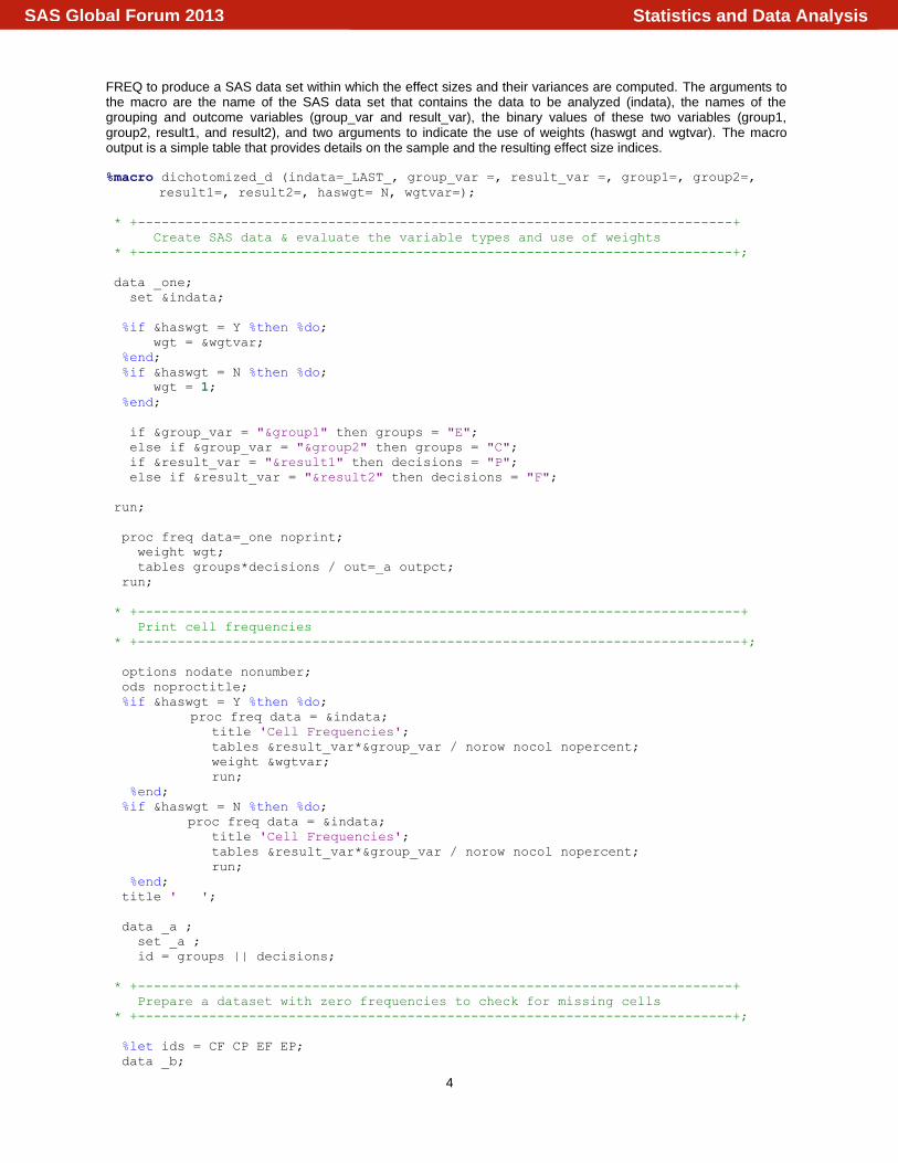
FREQ to produce a SAS data set within which the effect sizes and their variances are computed. The arguments to the macro are the name of the SAS data set that contains the data to be analyzed (indata), the names of the grouping and outcome variables (group_var and result_var), the binary values of these two variables (group1, group2, result1, and result2), and two arguments to indicate the use of weights (haswgt and wgtvar). The macro output is a simple table that provides details on the sample and the resulting effect size indices. %macro dichotomized_d (indata=_LAST_, group_var =, result_var =, group1=, group2=,
result1=, result2=, haswgt= N, wgtvar=);
* +---------------------------------------------------------------------------+
Create SAS data & evaluate the variable types and use of weights
* +---------------------------------------------------------------------------+;
data _one;
set &indata;
%if &haswgt = Y %then %do;
wgt = &wgtvar;
%end;
%if &haswgt = N %then %do;
wgt = 1;
%end;
if &group_var = "&group1" then groups = "E";
else if &group_var = "&group2" then groups = "C";
if &result_var = "&result1" then decisions = "P";
else if &result_var = "&result2" then decisions = "F";
run;
proc freq data=_one noprint;
weight wgt;
tables groups*decisions / out=_a outpct;
run;
* +----------------------------------------------------------------------------+
Print cell frequencies
* +----------------------------------------------------------------------------+;
options nodate nonumber;
ods noproctitle;
%if &haswgt = Y %then %do;
proc freq data = &indata;
title 'Cell Frequencies';
tables &result_var*&group_var / norow nocol nopercent;
weight &wgtvar;
run;
%end;
%if &haswgt = N %then %do;
proc freq data = &indata;
title 'Cell Frequencies';
tables &result_var*&group_var / norow nocol nopercent;
run;
%end;
title ' ';
data _a ;
set _a ;
id = groups || decisions;
* +---------------------------------------------------------------------------+
Prepare a dataset with zero frequencies to check for missing cells
* +---------------------------------------------------------------------------+;
%let ids = CF CP EF EP;
data _b;
Statistics and Data AnalysisSAS Global Forum 2013

5
%do v=1 %to 4;
%let idd = %scan(&ids,&v);
id = "&idd";
groups = substr("&idd",1,1);
decisions = substr("&idd",2,1);
count = .;
percent = .;
pct_row = .;
pct_col = .;
output;
%end;
run;
* +---------------------------------------------------------------------------+
Create a dataset with adjusted frequencies: if at least one cell has
frequency of zero, add 0.5 to each cell
* +---------------------------------------------------------------------------+;
proc sort data=_a; by id;
proc sort data=_b; by id;
data _two;
merge _b _a ;
by id;
cnt = .5;
proc sort data=_two; by cnt count; run;
data _two;
set _two;
retain mscnt;
by cnt;
if first.cnt then mscnt = count;
if mscnt = . then do;
if count = . then frq = cnt;
else frq = count + cnt;
end;
else frq = count;
if id = "CF" then call symputx("CFold",count);
if id = "CP" then call symputx("CPold",count);
if id = "EF" then call symputx("EFold",count);
if id = "EP" then call symputx("EPold",count);
if id = "CF" then call symputx("CF",frq);
if id = "CP" then call symputx("CP",frq);
if id = "EF" then call symputx("EF",frq);
if id = "EP" then call symputx("EP",frq);
* +---------------------------------------------------------------------------+
Calculate table elements using adjusted frequencies
* +---------------------------------------------------------------------------+;
data _three;
ocf = &CFold;
ocp = &CPold;
oef = &EFold;
oep = &EPold;
array actual(4) ocf ocp oef oep;
do i = 1 to 4;
if actual(i)=. then actual(i)=0;
end;
ncf = &CF;
ncp = &CP;
Statistics and Data AnalysisSAS Global Forum 2013
6
nef = &EF;
nep = &EP;
total = sum (of ncf ncp nef nep);
rowc = sum (of ncf ncp);
rowe = sum (of nef nep);
pcf = ncf/total;
pcp = ncp/total;
pef = nef/total;
pep = nep/total;
rcp = ncp/rowc;
rep = nep/rowe;
nc = ncf + ncp;
ne = nef + nep;
* +---------------------------------------------------------------------------+
Checking for invalid patterns of missing cells. If found, abort execution
and print message.
* +---------------------------------------------------------------------------+;
error = . ;
if ocf + ocp = 0 then error = 1;
if oef + oep = 0 then error = 1;
if ocf + oef = 0 then error = 1;
if ocp + oep = 0 then error = 1;
call symputx("error", error);
run;
%if &error = 1 %then %do;
%put "Please check data.";
data _null_;
file print notitles;
put @1 'Please check data.' /
'Effect size indices cannot be computed from this data table.';
return;
run;
%return;
%end;
data _three;
set _three;
* +---------------------------------------------------------------------------+
Computing the standardized proportion differences
* +---------------------------------------------------------------------------+;
s_prime = sqrt(((ne-1)*rep*(1-rep)+(nc-1)*rcp*(1-rcp))/(ne+nc-2));
d_p = (rep - rcp)/s_prime;
var_d_p =(ne + nc)/(ne*nc) + d_p**2/(2*(ne+nc));
* +---------------------------------------------------------------------------+
Computing standardized phi coefficient
* +---------------------------------------------------------------------------+;
phi = (nep*ncf-nef*ncp)/sqrt(ne*nc*(nep+ncp)*(nef+ncf));
d_phi = phi/sqrt(1-phi**2)*sqrt(((ne+nc-2)*(ne+nc))/(ne*nc));
var_d_phi = (ne+nc)/(ne*nc*(1-phi**2)**2);
* +---------------------------------------------------------------------------+
Computing standardized arcsin transformation d
* +---------------------------------------------------------------------------+;
d_asin = 2*arsin(sqrt(rep))-2*arsin(sqrt(rcp));
var_d_asin = 1/ne + 1/nc;
* +---------------------------------------------------------------------------+
Computing odds ratio based effect size
Statistics and Data AnalysisSAS Global Forum 2013
7
* +---------------------------------------------------------------------------+;
or = (rep*(1-rcp))/(rcp*(1-rep));
pi = constant('PI');
d_HH = log(or)*(sqrt(3)/pi);
var_d_HH = (3/pi**2)*(1/nep+1/ncp+1/nef+1/ncf);
* +---------------------------------------------------------------------------+
Computing Cox effect size
* +---------------------------------------------------------------------------+;
d_Cox = log(or)/1.65;
var_d_Cox = 0.367*(1/nep+1/ncp+1/nef+1/ncf);
* +---------------------------------------------------------------------------+
Computing probit effect size
* +---------------------------------------------------------------------------+;
d_probit = probit(rep) - probit(rcp);
var_d_probit = (2*pi*rep*(1-rep)*exp(probit(rep)**2))/ne +
(2*pi*rcp*(1-rcp)*exp(probit(rcp)**2))/nc;
* +---------------------------------------------------------------------------+
Computing biserial-phi coefficient
* +---------------------------------------------------------------------------+;
p_prime = pep + pcp;
q_prime = 1 - p_prime;
ordinate = pdf('NORMAL',PROBIT(p_prime));
phi_bis = sqrt(p_prime*q_prime)/ordinate*phi;
if phi_bis > .99 then phi_bis = .99;
if phi_bis < -.99 then phi_bis = -.99;
d_bis = (phi_bis/sqrt(1-phi_bis**2))*sqrt(((ne+nc-2)*(ne+nc))/(ne*nc));
var_d_bis = (p_prime*q_prime*(1-phi**2)*(ne+nc))/
(ordinate**2*ne*nc*(1-phi_bis**2)**3);
data _null_;
set _three;
* +---------------------------------------------------------------------------+
Print output using FILE PRINT
* +---------------------------------------------------------------------------+;
file print notitles;
put @1 'Estimated Effect Sizes for Dichotomized Variables' //
@1 'Index' @50 ' Value' @65 'Variance' /
@1 '------------------------------------' @49 '----------' @64 '----------' /
@1 'Standardized Proportion Difference' @50 d_p 8.4 @65 var_d_p 8.4 //
@1 'Standardized Phi' @50 d_phi 8.4 @65 var_d_phi 8.4 //
@1 'Arcsine D' @50 d_asin 8.4 @65 var_d_asin 8.4 //
@1 'dHH' @50 d_HH 8.4 @65 var_d_HH 8.4 //
@1 'Cox Effect Size' @50 d_Cox 8.4 @65 var_d_Cox 8.4 //
@1 'Probit Effect Size' @50 d_probit 8.4 @65 var_d_probit 8.4 //
@1 'Biserial-Phi Coefficient' @50 d_bis 8.4 @65 var_d_bis 8.4;
run;
* +---------------------------------------------------------------------------+
Clean up workspace: remove data sets created by the macro
* +---------------------------------------------------------------------------+;
proc datasets;
delete _one _two _three _a _b; quit;
%mend;
INVOKING THE MACRO
Statistics and Data AnalysisSAS Global Forum 2013

8
To better demonstrate how to use this macro, we will illustrate three datasets and associated calls to the macro. Dataset ONE uses alphanumeric variables for both treatment group and result. The arguments to the macro include the name of the SAS dataset (indata=one), the group variable (group_var=grp), and the result variable (result_var=decision). In addition, arguments specify the coding for grp and decision used in the dataset (group1=grp1, group2=grp2, result1=good, result2=bad).
data one;
input id grp $ decision $ ;
cards;
1 grp1 good
2 grp1 bad
3 grp2 good
4 grp2 good
.
.
;
%DICHOTOMIZED_d (indata=ONE,group_var=grp,result_var=decision,group1=grp1,
group2=grp2, result1=good, result2=bad);
For dataset TWO that uses numeric variables, the corresponding arguments to the macro should be the same as those for Dataset ONE, except for specifying the coding of the two numeric variables (group1=1, group2=2, result1=1, result2=2).
data two;
input id grp decision ;
cards;
1 1 1
2 1 2
3 2 1
4 2 1
.
.
;
%DICHOTOMIZED_d (indata=two,group_var=grp,result_var=decision,group1=1,group2=2,
result1=1,result2=2);
Dataset THREE illustrates the use of weights in calling the macro. This dataset has one row for each cell of the corresponding table, and a variable to indicate the number of observations in each cell. Because alphanumeric variables are used for grp and decision, the arguments are the same as those used for Dataset ONE, except for two additional arguments. One argument indicates that weights are used (haswgt=yes) and the other defines the name of the weight variable (wgtvar=frq). The output of the DICHOTOMIZED_D macro is presented in the next section.
data three;
input grp $ decision $ frq;
cards;
grp1 good 50
grp2 good 39
grp1 bad 20
grp2 bad 14
;
%DICHOTOMIZED_d (indata=three,group_var=grp,result_var=decision,group1=grp1,
group2=grp2,result1=good,result2=bad,haswgt=Y,wgtvar=frq);
OUTPUT FROM MACRO FOR DICHOTOMIZED EFFECT SIZES
Prior to displaying the effect sizes, the macro presents a two-dimensional frequency table providing the cell and marginal frequencies for the input data (Output 1). This table allows verification of the accuracy of the data being analyzed.
Statistics and Data AnalysisSAS Global Forum 2013

9
Cell Frequencies
Table of decision by grp
decision grp
Frequency‚grp1 ‚grp2 ‚ Total
ƒƒƒƒƒƒƒƒƒˆƒƒƒƒƒƒƒƒˆƒƒƒƒƒƒƒƒˆ
bad ‚ 4 ‚ 3 ‚ 7
ƒƒƒƒƒƒƒƒƒˆƒƒƒƒƒƒƒƒˆƒƒƒƒƒƒƒƒˆ
good ‚ 5 ‚ 7 ‚ 12
ƒƒƒƒƒƒƒƒƒˆƒƒƒƒƒƒƒƒˆƒƒƒƒƒƒƒƒˆ
Total 9 10 19
Output 1. A 2 by 2 Output Data File Generated Using PROC FREQ
The computed effect sizes and their variances are presented in a simple table (Output 2). In this example, the values of the estimated population effect sizes range between -.29 for Standardized Phi to -.38 for the Probit effect size. Note the Standardized Phi is the smallest effect size. The seven measures of effect size all fall within the same general range and are considered small population effect sizes (Cohen, 1977, 1988). The estimates for the variances of the effect sizes range between .21 for the Standardized Proportion Difference and Arcsine D and .38 for the Biserial-Phi coefficient. These are large variances; however, this is expected when the sample size is small.
Estimated Effect Sizes for Dichotomized Variables
Index Value Variance
------------------------------------ ---------- ----------
Standardized Proportion Difference -0.3029 0.2135
Standardized Phi -0.2865 0.2209
Arcsine D -0.3002 0.2111
dHH -0.3441 0.2815
Cox Effect Size -0.3783 0.3399
Probit Effect Size -0.3847 0.3495
Biserial-Phi Coefficient -0.3692 0.3778
Output 2. Estimated Effect Sizes for Dichotomized Variables
COMPARISON OF DICHOTOMIZED EFFECT SIZES FOR ACCURACY AND PRECISION
Kromrey and Bell (2012) investigated the accuracy and precision of the seven effect size indices using simulation methods. The Monte Carlo study investigated (a) overall sample size (n1 + n2 = 30, 60, 120, 240), (b) ratio of sample
sizes in the two groups (1:1, 1:2, 1:4), (c) population effect size (0, .2, .5, .8), (d) continuous score cut point for dichotomization (.10, .25, .40, .70), and (e) population variance ratio (1:1, 1:2, 1:3). For each condition, 100,000 replications were conducted. Using SAS/IML, normally distributed, continuous data were generated for two groups and the continuous variables were dichotomized at the specified cut points. In each sample, the standardized mean difference was computed prior to dichotomization and the seven effect size indices were computed after the data were dichotomized.
SIMULATION RESULTS
The overall distributions of statistical bias across all simulation conditions are presented as box and whisker plots in Figure 1. All seven indices tended to be negatively biased in their estimation of the effect size, yielding an effect size index that was smaller on average than the population effect size. Overall, the Cox, Probit, and biserial-phi indices evidenced notably smaller bias than the other indices, although the variability in the bias of the biserial-phi index was large relative to the others.
Statistics and Data AnalysisSAS Global Forum 2013

10
Figure 1. Distributions of Statistical Bias Estimates
In addition to the estimates of statistical bias, the sampling errors of the effect sizes were evaluation. The distributions of the empirical variances of the effect size indices across all conditions investigated in the simulation are presented in Figure 2. The average variances of the standardized proportion difference, the transformed phi coefficient, and the arcsine transformation were only slightly larger than the average variance of Cohen’s d effect size. In contrast, the other effect size indices yielded average variances that were nearly twice as large as these. Finally, the biserial-phi index evidenced exceptionally large sampling variance in many conditions.
The Root Mean Squared Error (RMSE) combines the bias and the standard error, resulting in the total error expected in a single sample estimate of the effect size. The distributions of RMSE across all simulation conditions are presented in Figure 3. In contrast to the statistical bias estimates, the smallest average RMSE values were obtained for the standardized proportion difference (dp), the transformed phi coefficient, and the arcsine transformation.
Notable also in Figure 3 is that the biserial-phi coefficient produces extremely large RMSE values in many conditions.
Figure 2. Distributions of Empirical Effect Size Variance Estimates
Statistics and Data AnalysisSAS Global Forum 2013

11
Figure 3. Distributions of RMSE Estimates
CONCLUSIONS
The macro Dichotomized_d provides calculations of the seven effect size indices described above, as well as their sampling variances. These indices have been proposed in the literature as methods to provide the estimated standardized mean difference after continuous data have been dichotomized. As noted in the simulation study conducted by Kromrey and Bell (2012), the statistical bias and sampling error for all seven of these indices compared to those of the effect size obtained prior to dichotomization (Cohen’s d), clearly demonstrate tenuous estimations of the effect size parameter after continuous variables have been dichotomized. This was especially problematic with smaller sample sizes and cut points in which the percentages were farther away from the median (e.g. .10 and .70 as opposed to .25 and .40). Working “backwards” to “undo” dichotomized continuous variables is a difficult task. A better choice is for researchers to also report the Cohen’s d value prior to the dichotomization. However, if the original data are not available, these indices provide a useful approximation.
The use of the Dichotomized_d macro is very easy; the researcher should simply read data using a regular SAS data step, then call the macro by specifying the data set name, the names of the grouping and outcome variables, the binary values of these two variables and two arguments to indicate the use of weights. The macro output is a simple table that provides details on the sample and the resulting effect size indices. Further, the macro may be easily modified to provide, for example, confidence intervals around the sample effect sizes (i.e., using the point estimates and estimated sampling variances) or to graph the effect size estimates with error bars (i.e., using SAS/GRAPH).
REFERENCES
American Psychological Association (2006). Publication manual of the American Psychological Association (6th ed.).
Washington, DC: Author.
Becker, G. & Thorndike, R. L. (1988). The biserial-phi correlation coefficient. Journal of Psychology, 122, 523-526.
Cohen, J. (1988). Statistical power analysis for the behavioral sciences (2nd
ed.). Hillsdale, NJ: Erlbaum.
Cox, D. R. (1970). Analysis of binary data. New York: Chapman & Hall.
Glass, G. V., McGaw, B., & Smith, M. L. (1981). Meta-analysis in social research. Beverly Hill, CA: Sage.
Hasselblad, V. & Hedges, L. V. (1995). Meta-analysis of screening and diagnostic tests. Psychological Bulletin, 117, 167-178.
Johnson, B. T. (1989). DSTAT: Software for the meta-analysis review of research [computer program and manual].
Hillsdale, NJ: Erlbaum.
Kromrey, J. D., & Bell, B. A. (2012). Effect size indices for dichotomized outcomes under variance heterogeneity: An empirical investigation of accuracy and precision. In JSM Proceedings. Social Statistics Section. Alexandria, VA: American Statistical Association.
Statistics and Data AnalysisSAS Global Forum 2013

12
Pedhazur, E. J., & Pedhazur Schmelkin, L. (1992). Measurement, Design, and Analysis: An Integral Approach. Hillsdale, NJ: Erlbaum.
Rosenthal, R. (1994). Parametric measures of effect size. In H. Cooper & L. V. Hedges (Eds.), Handbook of Research Synthesis (pp. 231-244). New York: Russell Sage Foundation.
Sanchez-Meca, J., Marin-Martinez, F., & Chacon-Moscoso, S. (2003). Effect size indices for dichotomized outcomes in meta-analysis. Psychological Methods, 8, 448-467.
SAS Institute Inc. (2008). SAS release 9.2 [computer program]. Carey, NC: SAS Institute Inc.
Wilkinson, L., & Task Force on Statistical Inference (1999). Statistical methods in psychological journals: Guidelines and Explanations. American Psychologist, 54, 594-604.
SAS and all other SAS Institute Inc. product or service names are registered trademarks or trademarks of SAS Institute Inc. in the USA and other countries. ® indicates USA registration.
Other brand and product names are trademarks of their respective companies.
CONTACT INFORMATION
Your comments and questions are valued and encouraged. Please contact: Patrice Rasmussen at: [email protected] University of South Florida, Tampa, FL 33620.
Statistics and Data AnalysisSAS Global Forum 2013
Related Documents