(where T 03 0 ¼ isentropic stagnation temperature at the diffuser outlet) or h c ¼ T 01 T 03 0 =T 01 2 1 T 03 2 T 01 Let P 01 be stagnation pressure at the compressor inlet and; P 03 is stagnation pressure at the diffuser exit. Then, using the isentropic P – T relationship, we get: P 03 P 01 ¼ T 03 0 T 01 g /ðg21Þ ¼ 1 þ h c ðT 03 2 T 01 Þ T 01 g /ðg21Þ ¼ 1 þ h c csU 2 2 C p T 01 g /ðg21Þ ð4:5Þ Equation (4.5) indicates that the pressure ratio also depends on the inlet temperature T 01 and impeller tip speed U 2 . Any lowering of the inlet temperature T 01 will clearly increase the pressure ratio of the compressor for a given work input, but it is not under the control of the designer. The centrifugal stresses in a rotating disc are proportional to the square of the rim. For single sided impellers of light alloy, U 2 is limited to about 460 m/s by the maximum allowable centrifugal stresses in the impeller. Such speeds produce pressure ratios of about 4:1. To avoid disc loading, lower speeds must be used for double-sided impellers. 4.7 DIFFUSER The designing of an efficient combustion system is easier if the velocity of the air entering the combustion chamber is as low as possible. Typical diffuser outlet velocities are in the region of 90 m/s. The natural tendency of the air in a diffusion process is to break away from the walls of the diverging passage, reverse its direction and flow back in the direction of the pressure gradient, as shown in Fig. 4.7. Eddy formation during air deceleration causes loss by reducing the maximum pressure rise. Therefore, the maximum permissible included angle of the vane diffuser passage is about 118. Any increase in this angle leads to a loss of efficiency due to Figure 4.7 Diffusing flow. Copyright 2003 by Marcel Dekker, Inc. All Rights Reserved

Welcome message from author
This document is posted to help you gain knowledge. Please leave a comment to let me know what you think about it! Share it to your friends and learn new things together.
Transcript

(where T030 ¼ isentropic stagnation temperature at the diffuser outlet) or
hc ¼ T01 T030=T01 2 1
� �
T03 2 T01
Let P01 be stagnation pressure at the compressor inlet and; P03 is stagnation
pressure at the diffuser exit. Then, using the isentropic P–T relationship, we get:
P03
P01
¼ T030
T01
� �g /ðg21Þ¼ 1þ hcðT03 2 T01Þ
T01
� �g /ðg21Þ
¼ 1þ hccsU2
2
Cp T01
� �g /ðg21Þð4:5Þ
Equation (4.5) indicates that the pressure ratio also depends on the inlet
temperature T01 and impeller tip speed U2. Any lowering of the inlet temperature
T01 will clearly increase the pressure ratio of the compressor for a given work
input, but it is not under the control of the designer. The centrifugal stresses in a
rotating disc are proportional to the square of the rim. For single sided impellers
of light alloy, U2 is limited to about 460m/s by the maximum allowable
centrifugal stresses in the impeller. Such speeds produce pressure ratios of about
4:1. To avoid disc loading, lower speeds must be used for double-sided impellers.
4.7 DIFFUSER
The designing of an efficient combustion system is easier if the velocity of the air
entering the combustion chamber is as low as possible. Typical diffuser outlet
velocities are in the region of 90m/s. The natural tendency of the air in a diffusion
process is to break away from thewalls of the diverging passage, reverse its direction
and flow back in the direction of the pressure gradient, as shown in Fig. 4.7. Eddy
formation during air deceleration causes loss by reducing the maximum pressure
rise. Therefore, the maximum permissible included angle of the vane diffuser
passage is about 118. Any increase in this angle leads to a loss of efficiency due to
Figure 4.7 Diffusing flow.
Chapter 4150
Copyright 2003 by Marcel Dekker, Inc. All Rights Reserved

boundary layer separation on the passage walls. It should also be noted that any
change from the design mass flow and pressure ratio would also result in a loss of
efficiency. The use of variable-angle diffuser vanes can control the efficiency loss.
The flow theory of diffusion, covered in Chapter 2, is applicable here.
4.8 COMPRESSIBILITY EFFECTS
If the relative velocity of a compressible fluid reaches the speed of sound in the fluid,
separation of flow causes excessive pressure losses. As mentioned earlier, diffusion
is a very difficult process and there is always a tendency for the flow to break away
from the surface, leading to eddy formation and reduced pressure rise. It is necessary
to control the Mach number at certain points in the flow to mitigate this problem.
The value of the Mach number cannot exceed the value at which shock waves
occur. The relative Mach number at the impeller inlet must be less than unity.
As shown in Fig. 4.8a, the air breakaway from the convex face of the
curved part of the impeller, and hence the Mach number at this point, will be very
important and a shock wave might occur. Now, consider the inlet velocity
triangle again (Fig. 4.5b). The relative Mach number at the inlet will be given by:
M1 ¼ V1ffiffiffiffiffiffiffiffiffiffiffigRT1
p ð4:6Þwhere T1 is the static temperature at the inlet.
It is possible to reduce the Mach number by introducing the prewhirl. The
prewhirl is given by a set of fixed intake guide vanes preceding the impeller.
As shown in Fig. 4.8b, relative velocity is reduced as indicated by the
dotted triangle. One obvious disadvantage of prewhirl is that the work capacity of
Figure 4.8 a) Breakaway commencing at the aft edge of the shock wave, and
b) Compressibility effects.
Centrifugal Compressors and Fans 151
Copyright 2003 by Marcel Dekker, Inc. All Rights Reserved

the compressor is reduced by an amount U1Cw1. It is not necessary to introduce
prewhirl down to the hub because the fluid velocity is low in this region due to
lower blade speed. The prewhirl is therefore gradually reduced to zero by
twisting the inlet guide vanes.
4.9 MACH NUMBER IN THE DIFFUSER
The absolute velocity of the fluid becomes a maximum at the tip of the impeller
and so the Mach number may well be in excess of unity. Assuming a perfect gas,
the Mach number at the impeller exit M2 can be written as:
M2 ¼ C2ffiffiffiffiffiffiffiffiffiffiffigRT2
p ð4:7ÞHowever, it has been found that as long as the radial velocity component (Cr2) is
subsonic, Mach number greater than unity can be used at the impeller tip without
loss of efficiency. In addition, supersonic diffusion can occur without the
formation of shock waves provided constant angular momentum is maintained
with vortex motion in the vaneless space. High Mach numbers at the inlet to the
diffuser vanes will also cause high pressure at the stagnation points on the diffuser
vane tips, which leads to a variation of static pressure around the circumference
of the diffuser. This pressure variation is transmitted upstream in a radial
direction through the vaneless space and causes cyclic loading of the impeller.
This may lead to early fatigue failure when the exciting frequency is of the same
order as one of the natural frequencies of the impeller vanes. To overcome this
concern, it is a common a practice to use prime numbers for the impeller vanes
and an even number for the diffuser vanes.
Figure 4.9 The theoretical centrifugal compressor characteristic.
Chapter 4152
Copyright 2003 by Marcel Dekker, Inc. All Rights Reserved

4.10 CENTRIFUGAL COMPRESSORCHARACTERISTICS
The performance of compressible flow machines is usually described in terms
of the groups of variables derived in dimensional analysis (Chapter 1). These
characteristics are dependent on other variables such as the conditions of
pressure and temperature at the compressor inlet and physical properties of
the working fluid. To study the performance of a compressor completely, it is
necessary to plot P03/P01 against the mass flow parameter mffiffiffiffiffiT01
pP01
for fixed
speed intervals of NffiffiffiffiffiT01
p . Figure 4.9 shows an idealized fixed speed
characteristic. Consider a valve placed in the delivery line of a compressor
running at constant speed. First, suppose that the valve is fully closed. Then
the pressure ratio will have some value as indicated by Point A. This
pressure ratio is available from vanes moving the air about in the impeller.
Now, suppose that the valve is opened and airflow begins. The diffuser
contributes to the pressure rise, the pressure ratio increases, and at Point B,
the maximum pressure occurs. But the compressor efficiency at this pressure
ratio will be below the maximum efficiency. Point C indicates the further
increase in mass flow, but the pressure has dropped slightly from the
maximum possible value. This is the design mass flow rate pressure ratio.
Further increases in mass flow will increase the slope of the curve until point
D. Point D indicates that the pressure rise is zero. However, the above-
described curve is not possible to obtain.
4.11 STALL
Stalling of a stage will be defined as the aerodynamic stall, or the breakaway of
the flow from the suction side of the blade airfoil. A multistage compressor may
operate stably in the unsurged region with one or more of the stages stalled, and
the rest of the stages unstalled. Stall, in general, is characterized by reverse flow
near the blade tip, which disrupts the velocity distribution and hence adversely
affects the performance of the succeeding stages.
Referring to the cascade of Fig. 4.10, it is supposed that some
nonuniformity in the approaching flow or in a blade profile causes blade B to
stall. The air now flows onto blade A at an increased angle of incidence due
to blockage of channel AB. The blade A then stalls, but the flow on blade C
is now at a lower incidence, and blade C may unstall. Therefore the stall
may pass along the cascade in the direction of lift on the blades. Rotating
stall may lead to vibrations resulting in fatigue failure in other parts of the
gas turbine.
Centrifugal Compressors and Fans 153
Copyright 2003 by Marcel Dekker, Inc. All Rights Reserved

4.12 SURGING
Surging is marked by a complete breakdown of the continuous steady flow
throughout the whole compressor, resulting in large fluctuations of flow with time
and also in subsequent mechanical damage to the compressor. The phenomenon
of surging should not be confused with the stalling of a compressor stage.
Figure 4.11 shows typical overall pressure ratios and efficiencies hc of a
centrifugal compressor stage. The pressure ratio for a given speed, unlike the
temperature ratio, is strongly dependent on mass flow rate, since the machine is
usually at its peak value for a narrow range of mass flows. When the compressor
is running at a particular speed and the discharge is gradually reduced, the
pressure ratio will first increase, peaks at a maximum value, and then decreased.
The pressure ratio is maximized when the isentropic efficiency has the
maximum value. When the discharge is further reduced, the pressure ratio drops
due to fall in the isentropic efficiency. If the downstream pressure does not drop
quickly there will be backflow accompanied by further decrease in mass flow. In
the mean time, if the downstream pressure drops below the compressor outlet
pressure, there will be increase in mass flow. This phenomenon of sudden drop
in delivery pressure accompanied by pulsating flow is called surging. The point
on the curve where surging starts is called the surge point. When the discharge
pipe of the compressor is completely choked (mass flow is zero) the pressure
ratio will have some value due to the centrifugal head produced by the impeller.
Figure 4.10 Mechanism of stall propagation.
Chapter 4154
Copyright 2003 by Marcel Dekker, Inc. All Rights Reserved

Between the zero mass flow and the surge point mass flow, the operation of the
compressor will be unstable. The line joining the surge points at different speeds
gives the surge line.
4.13 CHOKING
When the velocity of fluid in a passage reaches the speed of sound at any cross-
section, the flow becomes choked (air ceases to flow). In the case of inlet flow
passages, mass flow is constant. The choking behavior of rotating passages
Figure 4.11 Centrifugal compressor characteristics.
Centrifugal Compressors and Fans 155
Copyright 2003 by Marcel Dekker, Inc. All Rights Reserved

differs from that of the stationary passages, and therefore it is necessary to make
separate analysis for impeller and diffuser, assuming one dimensional, adiabatic
flow, and that the fluid is a perfect gas.
4.13.1 Inlet
When the flow is choked, C 2 ¼ a 2 ¼ gRT. Since h0 ¼ hþ 12C 2, then
CpT0 ¼ CpT þ 12g RT , and
T
T0
¼ 1þ gR
2Cp
� �21
¼ 2
gþ 1ð4:8Þ
Assuming isentropic flow, we have:
r
r0
� �¼ P
P0
� �T0
T
� �¼ 1þ 1
2g2 1� �
M 2
� � 12gð Þ= g21ð Þð4:9Þ
and when C ¼ a, M ¼ 1, so that:
r
r0
� �¼ 2
gþ 1� �
" #1= g21ð Þð4:10Þ
Using the continuity equation,_mA
� � ¼ rC ¼ r gRT 1=2
, we have
_m
A
� �¼ r0a0
2
gþ 1
� � gþ1ð Þ=2 g21ð Þð4:11Þ
where (r0 and a0 refer to inlet stagnation conditions, which remain unchanged.
The mass flow rate at choking is constant.
4.13.2 Impeller
When choking occurs in the impeller passages, the relative velocity equals the
speed of sound at any section. The relative velocity is given by:
V 2 ¼ a2 ¼ gRT
and T01 ¼ T þ gRT
2Cp
� �2
U 2
2Cp
Therefore,
T
T01
� �¼ 2
gþ 1
� �1þ U 2
2CpT01
� �ð4:12Þ
Chapter 4156
Copyright 2003 by Marcel Dekker, Inc. All Rights Reserved

Using isentropic conditions,
r
r01
� �¼ T
T01
� �1= g21ð Þand; from the continuity equation:
_m
A
� �¼ r0a01
T
T01
� �ðgþ1Þ=2ðg21Þ
¼ r01a012
gþ 1
� �1þ U 2
2CpT01
� �� �ðgþ1Þ=2ðg21Þ
¼ r01a012þ g2 1
� �U 2=a201
gþ 1
� �ðgþ1Þ=2ðg21Þ ð4:13Þ
Equation (4.13) indicates that for rotating passages, mass flow is dependent on
the blade speed.
4.13.3 Diffuser
For choking in the diffuser, we use the stagnation conditions for the diffuser and
not the inlet. Thus:
_m
A
� �¼ r02a02
2
gþ 1
� � gþ1ð Þ=2 g21ð Þð4:14Þ
It is clear that stagnation conditions at the diffuser inlet are dependent on the
impeller process.
Illustrative Example 4.1: Air leaving the impeller with radial velocity
110m/s makes an angle of 258300 with the axial direction. The impeller tip speed
is 475m/s. The compressor efficiency is 0.80 and the mechanical efficiency
is 0.96. Find the slip factor, overall pressure ratio, and power required to drive the
compressor. Neglect power input factor and assume g ¼ 1.4, T01 ¼ 298K, and
the mass flow rate is 3 kg/s.
Solution:
From the velocity triangle (Fig. 4.12),
tan b2
� � ¼ U2 2 Cw2
Cr2
tan 25:58ð Þ ¼ 4752 Cw2
110
Therefore, Cw2 ¼ 422:54m/s.
Centrifugal Compressors and Fans 157
Copyright 2003 by Marcel Dekker, Inc. All Rights Reserved

Now, s ¼ Cw2U2
¼ 422:54475
¼ 0:89
The overall pressure ratio of the compressor:
P03
P01
¼ 1þhcscU22
CpT01
� �g= g21ð Þ¼ 1þð0:80Þð0:89Þð4752Þ
ð1005Þð298Þ� �3:5
¼ 4:5
The theoretical power required to drive the compressor:
P¼ mscU 22
1000
� �kW¼ ð3Þð0:89Þð4752Þ
1000
� �¼ 602:42kW
Using mechanical efficiency, the actual power required to drive the
compressor is: P ¼ 602.42/0.96 ¼ 627.52 kW.
Illustrative Example 4.2: The impeller tip speed of a centrifugal
compressor is 370m/s, slip factor is 0.90, and the radial velocity component at the
exit is 35m/s. If the flow area at the exit is 0.18m2 and compressor efficiency is
0.88, determine the mass flow rate of air and the absolute Mach number at the
impeller tip. Assume air density ¼ 1.57 kg/m3 and inlet stagnation temperature
is 290K. Neglect the work input factor. Also, find the overall pressure ratio of the
compressor.
Solution:
Slip factor: s ¼ Cw2
U2Therefore: Cw2 ¼ U2s ¼ (0.90)(370) ¼ 333m/s
The absolute velocity at the impeller exit:
C2 ¼ffiffiffiffiffiffiffiffiffiffiffiffiffiffiffiffiffiffiffiffiC2r2 þ C2
v2
q¼
ffiffiffiffiffiffiffiffiffiffiffiffiffiffiffiffiffiffiffiffiffiffi3332 þ 352
p¼ 334:8m/s
The mass flow rate of air: _m ¼ r2A2Cr2 ¼ 1:57*0:18*35 ¼ 9:89 kg/s
Figure 4.12 Velocity triangle at the impeller tip.
Chapter 4158
Copyright 2003 by Marcel Dekker, Inc. All Rights Reserved

The temperature equivalent of work done (neglecting c):
T02 2 T01 ¼ sU22
Cp
Therefore, T02 ¼ T01 þ sU22
Cp¼ 290þ ð0:90Þð3702Þ
1005¼ 412:6K
The static temperature at the impeller exit,
T2 ¼ T02 2C22
2Cp
¼ 412:62334:82
ð2Þð1005Þ ¼ 356:83K
The Mach number at the impeller tip:
M2 ¼ C2ffiffiffiffiffiffiffiffiffiffiffigRT2
p ¼ 334:8ffiffiffiffiffiffiffiffiffiffiffiffiffiffiffiffiffiffiffiffiffiffiffiffiffiffiffiffiffiffiffiffiffiffiffiffiffið1:4Þð287Þð356:83Þp ¼ 0:884
The overall pressure ratio of the compressor (neglecting c):
P03
P01
¼ 1þ hcscU22
CpT01
� �3:5¼ 1þ ð0:88Þð0:9Þð3702Þ
ð1005Þð290Þ� �3:5
¼ 3:0
Illustrative Example 4.3: A centrifugal compressor is running at
16,000 rpm. The stagnation pressure ratio between the impeller inlet and outlet
is 4.2. Air enters the compressor at stagnation temperature of 208C and 1 bar.
If the impeller has radial blades at the exit such that the radial velocity at the exit
is 136m/s and the isentropic efficiency of the compressor is 0.82. Draw the
velocity triangle at the exit (Fig. 4.13) of the impeller and calculate slip. Assume
axial entrance and rotor diameter at the outlet is 58 cm.
Figure 4.13 Velocity triangle at exit.
Centrifugal Compressors and Fans 159
Copyright 2003 by Marcel Dekker, Inc. All Rights Reserved

Solution:
Impeller tip speed is given by:
U2 ¼ pDN
60¼ ðpÞð0:58Þð16000Þ
60¼ 486m/s
Assuming isentropic flow between impeller inlet and outlet, then
T020 ¼ T01 4:2ð Þ0:286 ¼ 441:69K
Using compressor efficiency, the actual temperature rise
T02 2 T01 ¼ T020 2 T01
� �
hc
¼ 441:692 293ð Þ0:82
¼ 181:33K
Since the flow at the inlet is axial, Cw1 ¼ 0
W ¼ U2Cw2 ¼ Cp T02 2 T01ð Þ ¼ 1005ð181:33ÞTherefore: Cw2 ¼ 1005 181:33ð Þ
486¼ 375m/s
Slip ¼ 486–375 ¼ 111m/s
Slip factor: s ¼ Cw2
U2
¼ 375
486¼ 0:772
Illustrative Example 4.4: Determine the adiabatic efficiency, temperature
of the air at the exit, and the power input of a centrifugal compressor from the
following given data:
Impeller tip diameter ¼ 1m
Speed ¼ 5945 rpm
Mass flow rate of air ¼ 28 kg/s
Static pressure ratio p3/p1 ¼ 2:2
Atmospheric pressure ¼ 1 bar
Atmospheric temperature ¼ 258C
Slip factor ¼ 0:90
Neglect the power input factor.
Solution:
The impeller tip speed is given by:
U2 ¼ pDN60
¼ ðpÞð1Þð5945Þ60
¼ 311m/s
The work input: W ¼ sU22 ¼ ð0:9Þð3112Þ
1000¼ 87 kJ/kg
Chapter 4160
Copyright 2003 by Marcel Dekker, Inc. All Rights Reserved

Using the isentropic P–T relation and denoting isentropic temperature by
T30, we get:
T30 ¼ T1
P3
P1
� �0:286
¼ ð298Þð2:2Þ0:286 ¼ 373:38K
Hence the isentropic temperature rise:
T30 2 T1 ¼ 373:382 298 ¼ 75:38K
The temperature equivalent of work done:
T3 2 T1 ¼ W
Cp
� �¼ 87/1:005 ¼ 86:57K
The compressor adiabatic efficiency is given by:
hc ¼ T30 2 T1
� �
T3 2 T1ð Þ ¼ 75:38
86:57¼ 0:871 or 87:1%
The air temperature at the impeller exit is:
T3 ¼ T1 þ 86:57 ¼ 384:57K
Power input:
P ¼ _mW ¼ ð28Þð87Þ ¼ 2436 kW
Illustrative Example 4.5: A centrifugal compressor impeller rotates at
9000 rpm. If the impeller tip diameter is 0.914m and a2 ¼ 208, calculate
the following for operation in standard sea level atmospheric conditions: (1) U2,
(2) Cw2, (3) Cr2, (4) b2, and (5) C2.
1. Impeller tip speed is given by U2 ¼ pDN60
¼ ðpÞð0:914Þð9000Þ60
¼ 431m/s
2. Since the exit is radial and no slip, Cw2 ¼ U2 ¼ 431m/s
3. From the velocity triangle,
Cr2 ¼ U2 tan(a2) ¼ (431) (0.364) ¼ 156.87m/s
4. For radial exit, relative velocity is exactly perpendicular to rotational
velocity U2. Thus the angle b2 is 908 for radial exit.5. Using the velocity triangle (Fig. 4.14),
C2 ¼ffiffiffiffiffiffiffiffiffiffiffiffiffiffiffiffiffiffiU2
2 þ C2r2
q¼
ffiffiffiffiffiffiffiffiffiffiffiffiffiffiffiffiffiffiffiffiffiffiffiffiffiffiffiffiffiffiffi4312 þ 156:872
p¼ 458:67m/s
Illustrative Example 4.6: A centrifugal compressor operates with no
prewhirl is runwith a rotor tip speed of 457m/s. IfCw2 is 95%ofU2 andhc ¼ 0.88,
Centrifugal Compressors and Fans 161
Copyright 2003 by Marcel Dekker, Inc. All Rights Reserved

calculate the following for operation in standard sea level air: (1) pressure ratio, (2)
work input per kg of air, and (3) the power required for a flow of 29 k/s.
Solution:
1. The pressure ratio is given by (assuming s ¼ c ¼ 1):
P03
P01
¼ 1þ hcscU22
CpT01
� �g= g21ð Þ
¼ 1þ ð0:88Þð0:95Þð4572Þð1005Þð288Þ
� �3:5¼ 5:22
2. The work per kg of air
W ¼ U2Cw2 ¼ ð457Þð0:95Þð457Þ ¼ 198:4 kJ/kg
3. The power for 29 kg/s of air
P ¼ _mW ¼ ð29Þð198:4Þ ¼ 5753:6 kW
Illustrative Example 4.7: A centrifugal compressor is running at
10,000 rpm and air enters in the axial direction. The inlet stagnation temperature
of air is 290K and at the exit from the impeller tip the stagnation temperature is
440K. The isentropic efficiency of the compressor is 0.85, work input factor
c ¼ 1.04, and the slip factor s ¼ 0.88. Calculate the impeller tip diameter,
overall pressure ratio, and power required to drive the compressor per unit mass
flow rate of air.
Figure 4.14 Velocity triangle at impeller exit.
Chapter 4162
Copyright 2003 by Marcel Dekker, Inc. All Rights Reserved

Solution:
Temperature equivalent of work done:
T02 2 T01 ¼ scU22
Cp
orð0:88Þð1:04ÞðU2
2Þ1005
:
Therefore; U2 ¼ 405:85m/s
and D ¼ 60U2
pN¼ ð60Þð405:85Þ
ðpÞð10; 000Þ ¼ 0:775m
The overall pressure ratio is given by:
P03
P01
¼ 1þ hcscU22
CpT01
� �g= g21ð Þ
¼ 1þ ð0:85Þð0:88Þð1:04Þð405:852Þð1005Þð290Þ
� �3:5¼ 3:58
Power required to drive the compressor per unit mass flow:
P ¼ mcsU22 ¼
ð1Þð0:88Þð1:04Þð405:852Þ1000
¼ 150:75 kW
Design Example 4.8: Air enters axially in a centrifugal compressor at a
stagnation temperature of 208C and is compressed from 1 to 4.5 bars. The
impeller has 19 radial vanes and rotates at 17,000 rpm. Isentropic efficiency of the
compressor is 0.84 and the work input factor is 1.04. Determine the overall
diameter of the impeller and the power required to drive the compressor when the
mass flow is 2.5 kg/s.
Solution:
Since the vanes are radial, using the Stanitz formula to find the slip factor:
s ¼ 120:63p
n¼ 12
0:63p
19¼ 0:8958
The overall pressure ratio
P03
P01
¼ 1þ hcscU22
CpT01
� �g= g21ð Þ; or 4:5
¼ 1þ ð0:84Þð0:8958Þð1:04ÞðU22Þ
ð1005Þð293Þ� �3:5
; soU2 ¼ 449:9m/s
The impeller diameter, D ¼ 60U2
pN¼ ð60Þð449:9Þ
pð17; 000Þ ¼ 0:5053m ¼ 50:53 cm.
Centrifugal Compressors and Fans 163
Copyright 2003 by Marcel Dekker, Inc. All Rights Reserved

The work done on the air W ¼ csU22
1000¼ ð0:8958Þð1:04Þð449:92Þ
1000¼
188:57 kJ/kg
Power required to drive the compressor: P ¼ _mW ¼ ð2:5Þð188:57Þ ¼471:43 kW
Design Example 4.9: Repeat problem 4.8, assuming the air density at the
impeller tip is 1.8 kg/m3 and the axial width at the entrance to the diffuser is
12mm. Determine the radial velocity at the impeller exit and the absolute Mach
number at the impeller tip.
Solution:
Slip factor: s ¼ Cw2
U2
; orCw2 ¼ ð0:8958Þð449:9Þ ¼ 403m/s
Using the continuity equation,
_m ¼ r2A2Cr2 ¼ r22pr2b2Cr2
where:
b2 ¼ axial width
r2 ¼ radius
Therefore:
Cr2 ¼ 2:5
ð1:8Þð2pÞð0:25Þð0:012Þ ¼ 73:65m/s
Absolute velocity at the impeller exit
C2 ¼ffiffiffiffiffiffiffiffiffiffiffiffiffiffiffiffiffiffiffiffiC2r2 þ C2
w2
q¼
ffiffiffiffiffiffiffiffiffiffiffiffiffiffiffiffiffiffiffiffiffiffiffiffiffiffiffiffi73:652 þ 4032
p¼ 409:67m/s
The temperature equivalent of work done:
T02 2 T01 ¼ 188:57/Cp ¼ 188:57/1:005 ¼ 187:63K
Therefore, T02 ¼ 293 þ 187.63 ¼ 480.63K
Hence the static temperature at the impeller exit is:
T2 ¼ T02 2C22
2Cp
¼ 480:632409:672
ð2Þð1005Þ ¼ 397K
Now, the Mach number at the impeller exit is:
M2 ¼ C2ffiffiffiffiffiffiffiffiffiffiffigRT2
p ¼ 409:67ffiffiffiffiffiffiffiffiffiffiffiffiffiffiffiffiffiffiffiffiffiffiffiffiffiffiffiffiffið1:4Þð287Þð397p Þ ¼ 1:03
Design Example 4.10: A centrifugal compressor is required to deliver
8 kg/s of air with a stagnation pressure ratio of 4 rotating at 15,000 rpm. The air
enters the compressor at 258C and 1 bar. Assume that the air enters axially with
velocity of 145m/s and the slip factor is 0.89. If the compressor isentropic
Chapter 4164
Copyright 2003 by Marcel Dekker, Inc. All Rights Reserved

efficiency is 0.89, find the rise in stagnation temperature, impeller tip speed,
diameter, work input, and area at the impeller eye.
Solution:
Inlet stagnation temperature:
T01 ¼ Ta þ C21
2Cp
¼ 298þ 1452
ð2Þð1005Þ ¼ 308:46K
Using the isentropic P–T relation for the compression process,
T030 ¼ T01
P03
P01
� � g21ð Þ=g¼ ð308:46Þ 4ð Þ0:286 ¼ 458:55K
Using the compressor efficiency,
T02 2 T01 ¼ T020 2 T01
� �
hc
¼ 458:552 308:46ð Þ0:89
¼ 168:64K
Hence, work done on the air is given by:
W ¼ Cp T02 2 T01ð Þ ¼ ð1:005Þð168:64Þ ¼ 169:48 kJ/kg
But,
W ¼ sU22 ¼
ð0:89ÞðU2Þ1000
; or :169:48 ¼ 0:89U22/1000
or:
U2 ¼ffiffiffiffiffiffiffiffiffiffiffiffiffiffiffiffiffiffiffiffiffiffiffiffiffiffiffiffiffiffið1000Þð169:48Þ
0:89
r
¼ 436:38m/s
Hence, the impeller tip diameter
D ¼ 60U2
pN¼ ð60Þð436:38Þ
p ð15; 000Þ ¼ 0:555m
The air density at the impeller eye is given by:
r1 ¼ P1
RT1
¼ ð1Þð100Þð0:287Þð298Þ ¼ 1:17 kg/m3
Using the continuity equation in order to find the area at the impeller eye,
A1 ¼_m
r1C1
¼ 8
ð1:17Þð145Þ ¼ 0:047m2
The power input is:
P ¼ _m W ¼ ð8Þð169:48Þ ¼ 1355:24 kW
Centrifugal Compressors and Fans 165
Copyright 2003 by Marcel Dekker, Inc. All Rights Reserved

Design Example 4.11: The following data apply to a double-sided
centrifugal compressor (Fig. 4.15):
Impeller eye tip diameter : 0:28m
Impeller eye root diameter : 0:14m
Impeller tip diameter: 0:48m
Mass flow of air: 10 kg/s
Inlet stagnation temperature : 290K
Inlet stagnation pressure : 1 bar
Air enters axially with velocity: 145m/s
Slip factor : 0:89
Power input factor: 1:03
Rotational speed: 15; 000 rpm
Calculate (1) the impeller vane angles at the eye tip and eye root, (2) power
input, and (3) the maximum Mach number at the eye.
Solution:
(1) Let Uer be the impeller speed at the eye root. Then the vane angle at
the eye root is:
aer ¼ tan21 Ca
Uer
� �
and
Uer ¼ pDerN
60¼ pð0:14Þð15; 000Þ
60¼ 110m/s
Hence, the vane angle at the impeller eye root:
aer ¼ tan21 Ca
Uer
� �¼ tan21 145
110
� �¼ 52848
0
Figure 4.15 The velocity triangle at the impeller eye.
Chapter 4166
Copyright 2003 by Marcel Dekker, Inc. All Rights Reserved

Impeller velocity at the eye tip:
Uet ¼ pDetN
60¼ pð0:28Þð15; 000Þ
60¼ 220m/s
Therefore vane angle at the eye tip:
aet ¼ tan21 Ca
Uet
� �¼ tan21 145
220
� �¼ 33823
0
(2) Work input:
W ¼ _mcsU22 ¼ ð10Þð0:819Þð1:03U2
2Þ
but:
U2 ¼ pD2N
60¼ pð0:48Þð15; 000Þ
60¼ 377:14m/s
Hence,
W ¼ ð10Þð0:89Þð1:03Þð377:142Þ1000
¼ 1303:86 kW
(3) The relative velocity at the eye tip:
V1 ¼ffiffiffiffiffiffiffiffiffiffiffiffiffiffiffiffiffiffiU2
et þ C2a
q¼
ffiffiffiffiffiffiffiffiffiffiffiffiffiffiffiffiffiffiffiffiffiffiffiffiffi2202 þ 1452
p¼ 263:5m/s
Hence, the maximum relative Mach number at the eye tip:
M1 ¼ V1ffiffiffiffiffiffiffiffiffiffiffigRT1
p ;
where T1 is the static temperature at the inlet
T1 ¼ T01 2C21
2Cp
¼ 29021452
ð2Þð1005Þ ¼ 279:54K
The Mach number at the inlet then is:
M1 ¼ V1ffiffiffiffiffiffiffiffiffiffiffigRT1
p ¼ 263/5ffiffiffiffiffiffiffiffiffiffiffiffiffiffiffiffiffiffiffiffiffiffiffiffiffiffiffiffiffiffiffiffiffiffiffið1:4Þð287Þð279:54p Þ ¼ 0:786
Design Example 4.12: Recalculate the maximum Mach number at the
impeller eye for the same data as in the previous question, assuming prewhirl
angle of 208.
Centrifugal Compressors and Fans 167
Copyright 2003 by Marcel Dekker, Inc. All Rights Reserved

Solution:
Figure 4.16 shows the velocity triangle with the prewhirl angle.
From the velocity triangle:
C1 ¼ 145
cosð208Þ ¼ 154:305m/s
Equivalent dynamic temperature:
C21
2Cp
¼ 154:3052
ð2Þð1005Þ ¼ 11:846K
Cw1 ¼ tanð208ÞCa1 ¼ ð0:36Þð145Þ ¼ 52:78m/s
Relative velocity at the inlet:
V21 ¼ C2
a þ Ue 2 Cw1ð Þ2¼ 1452 þ ð2202 52:78Þ2; orV1
¼ 221:3m/s
Therefore the static temperature at the inlet:
T1 ¼ T01 2C21
2Cp
¼ 2902 11:846 ¼ 278:2K
Hence,
M1 ¼ V1ffiffiffiffiffiffiffiffiffiffiffigRT1
p ¼ 221:3ffiffiffiffiffiffiffiffiffiffiffiffiffiffiffiffiffiffiffiffiffiffiffiffiffiffiffiffiffiffiffiffiffið1:4Þð287Þð278:2p Þ ¼ 0:662
Note the reduction in Mach number due to prewhirl.
Figure 4.16 The velocity triangle at the impeller eye.
Chapter 4168
Copyright 2003 by Marcel Dekker, Inc. All Rights Reserved

Design Example 4.13: The following data refers to a single-sided
centrifugal compressor:
Ambient Temperature: 288K
Ambient Pressure: 1 bar
Hub diameter : 0:125m
Eye tip diameter: 0:25m
Mass flow: 5:5 kg/s
Speed: 16; 500 rpm
Assume zero whirl at the inlet and no losses in the intake duct. Calculate the
blade inlet angle at the root and tip and the Mach number at the eye tip.
Solution:
Let: rh ¼ hub radius
rt ¼ tip radius
The flow area of the impeller inlet annulus is:
A1 ¼ p r2t 2 r2h� � ¼ p 0:1252 2 0:06252
� � ¼ 0:038m2
Axial velocity can be determined from the continuity equation but since the
inlet density (r1) is unknown a trial and error method must be followed.
Assuming a density based on the inlet stagnation condition,
r1 ¼ P01
RT01
¼ ð1Þð105Þð287Þð288Þ ¼ 1:21 kg/m3
Using the continuity equation,
Ca ¼_m
r1A1
¼ 5:5
ð1:21Þð0:038Þ ¼ 119:6m/s
Since the whirl component at the inlet is zero, the absolute velocity at the
inlet is C1 ¼ Ca.
The temperature equivalent of the velocity is:
C21
2Cp
¼ 119:62
ð2Þð1005Þ ¼ 7:12K
Therefore:
T1 ¼ T01 2C21
2Cp
¼ 2882 7:12 ¼ 280:9K
Centrifugal Compressors and Fans 169
Copyright 2003 by Marcel Dekker, Inc. All Rights Reserved

Using isentropic P–T relationship,
P1
P01
¼ T1
T01
� �g= g21ð Þ; or P1 ¼ 105
280:9
288
� �3:5
¼ 92 kPa
and:
r1 ¼ P1
RT1
¼ ð92Þð103Þð287Þð280:9Þ ¼ 1:14 kg/m3; and
Ca ¼ 5:5
ð1:14Þð0:038Þ ¼ 126:96m/s
Therefore:
C21
2Cp
¼ ð126:96Þ22ð1005Þ ¼ 8:02K
T1 ¼ 2882 8:02 ¼ 279:988K
P1 ¼ 105279:98
288
� �3:5
¼ 90:58 kPa
r1 ¼ ð90:58Þð103Þð287Þð279:98Þ ¼ 1:13 kg/m3
Further iterations are not required and the value of r1 ¼ 1.13 kg/m3 may be
taken as the inlet density and Ca ¼ C1 as the inlet velocity. At the eye tip:
Uet ¼ 2pretN
60¼ 2p ð0:125Þð16; 500Þ
60¼ 216m/s
The blade angle at the eye tip:
bet ¼ tan21 Uet
Ca
� �¼ tan21 216
126:96
� �¼ 59:568
At the hub,
Ueh ¼ 2pð0:0625Þð16; 500Þ60
¼ 108m/s
The blade angle at the hub:
beh ¼ tan21 108
126:96
� �¼ 40:398
Chapter 4170
Copyright 2003 by Marcel Dekker, Inc. All Rights Reserved

The Mach number based on the relative velocity at the eye tip using the
inlet velocity triangle is:
V1 ¼ffiffiffiffiffiffiffiffiffiffiffiffiffiffiffiffiffiC2a þ U2
1
q¼
ffiffiffiffiffiffiffiffiffiffiffiffiffiffiffiffiffiffiffiffiffiffiffiffiffiffiffiffiffiffiffi126:962 þ 2162
p; orV1 ¼ 250:6m/s
The relative Mach number
M ¼ V1ffiffiffiffiffiffiffiffiffiffiffigRT1
p ¼ 250:6ffiffiffiffiffiffiffiffiffiffiffiffiffiffiffiffiffiffiffiffiffiffiffiffiffiffiffiffiffiffiffiffiffiffiffið1:4Þð287Þð279:98p Þ ¼ 0:747
Design Example 4.14:A centrifugal compressor compresses air at ambient
temperature and pressure of 288K and 1 bar respectively. The impeller tip speed
is 364m/s, the radial velocity at the exit from the impeller is 28m/s, and the slip
factor is 0.89. Calculate the Mach number of the flow at the impeller tip. If the
impeller total-to-total efficiency is 0.88 and the flow area from the impeller is
0.085m2, calculate the mass flow rate of air. Assume an axial entrance at the
impeller eye and radial blades.
Solution:
The absolute Mach number of the air at the impeller tip is:
M2 ¼ C2ffiffiffiffiffiffiffiffiffiffiffigRT2
p
where T2 is the static temperature at the impeller tip. Let us first calculate
C2 and T2.
Slip factor:
s ¼ Cw2
U2
Or:
Cw2 ¼ sU2 ¼ ð0:89Þð364Þ ¼ 323:96m/s
From the velocity triangle,
C22 ¼ C2
r2 þ C2w2 ¼ 282 þ 323:962 ¼ ð1:06Þð105Þm2/s2
With zero whirl at the inlet
W
m¼ sU2
2 ¼ Cp T02 2 T01ð ÞHence,
T02 ¼ T01 þ sU22
Cp
¼ 288þ ð0:89Þð3642Þ1005
¼ 405:33K
Centrifugal Compressors and Fans 171
Copyright 2003 by Marcel Dekker, Inc. All Rights Reserved

Static Temperature
T2 ¼ T02 2C22
2Cp
¼ 405:332106000
ð2Þð1005Þ ¼ 352:6K
Therefore,
M2 ¼ ð1:06Þð105Þð1:4Þð287Þð352:6Þ
� �12
¼ 0:865
Using the isentropic P–T relation:
P02
P01
� �¼ 1þ hc
T02
T01
2 1
� �� �g= g21ð Þ
¼ 1þ 0:88405:33
2882 1
� �� �3:5¼ 2:922
P2
P02
� �¼ T2
T02
� �3:5
¼ 352:6
405:33
� �3:5
¼ 0:614
Therefore,
P2 ¼ P2
P02
� �P02
P01
� �P01
¼ ð0:614Þð2:922Þð1Þð100Þ¼ 179:4 kPa
r2 ¼ 179:4ð1000Þ287ð352:6Þ ¼ 1:773 kg/m3
Mass flow:
_m ¼ ð1:773Þð0:085Þð28Þ ¼ 4:22 kg/s
Design Example 4.15: The impeller of a centrifugal compressor rotates at
15,500 rpm, inlet stagnation temperature of air is 290K, and stagnation pressure
at inlet is 101 kPa. The isentropic efficiency of impeller is 0.88, diameter of the
impellar is 0.56m, axial depth of the vaneless space is 38mm, and width of the
vaneless space is 43mm. Assume ship factor as 0.9, power input factor 1.04, mass
flow rate as 16 kg/s. Calculate
1. Stagnation conditions at the impeller outlet, assume no fore whirl at the
inlet,
2. Assume axial velocity approximately equal to 105m/s at the impeller
outlet, calculate the Mach number and air angle at the impeller outlet,
Chapter 4172
Copyright 2003 by Marcel Dekker, Inc. All Rights Reserved

3. The angle of the diffuser vane leading edges and the Mach number at
this radius if the diffusion in the vaneless space is isentropic.
Solution:
1. Impeller tip speed
U2 ¼ pD2N
60¼ p £ 0:56 £ 15500
60
U2 ¼ 454:67m/s
Overall stagnation temperature rise
T03 2 T01 ¼ csU22
1005¼ 1:04 £ 0:9 £ 454:672
1005
¼ 192:53K
Since T03 ¼ T02Therefore, T02 2 T01 ¼ 192.53K and T02 ¼ 192.53 þ 290 ¼ 482.53K
Now pressure ratio for impeller
p02
p01¼ T02
T01
� �3:5
¼ 482:53
290
� �3:5
¼ 5:94
then, p02 ¼ 5.94 £ 101 ¼ 600 KPa
2.
s ¼ Cw2
U2
Cw2 ¼ sU2
orCw2 ¼ 0:9 £ 454:67 ¼ 409m/s
Let Cr2 ¼ 105m/s
Outlet area normal to periphery
A2 ¼ pD2 £ impeller depth
¼ p £ 0:56 £ 0:038
A2 ¼ 0:0669m2
From outlet velocity triangle
C 22 ¼ C 2
r2 þ C 2w2
¼ 1052 þ 4092
C 22 ¼ 178306
Centrifugal Compressors and Fans 173
Copyright 2003 by Marcel Dekker, Inc. All Rights Reserved

i:e: C2 ¼ 422:26m/s
T2 ¼ T02 2C 2
2
2Cp
¼ 482:532422:262
2 £ 1005
T2 ¼ 393:82K
Using isentropic P–T relations
P2 ¼ P02
T2
T02
� � gg21
¼ 600393:82
482:53
� �3:5
¼ 294:69 kPa
From equation of state
r2 ¼ P2
RT2
¼ 293:69 £ 103
287 £ 393:82¼ 2:61 kg/m3
The equation of continuity gives
Cr2 ¼_m
A2P2
¼ 16
0:0669 £ 2:61¼ 91:63m/s
Thus, impeller outlet radial velocity ¼ 91.63m/s
Impeller outlet Mach number
M2 ¼ C2ffiffiffiffiffiffiffiffiffiffiffigRT2
p ¼ 422:26
1:4 £ 287 £ 393:82ð Þ0:5
M2 ¼ 1:06
From outlet velocity triangle
Cosa2 ¼ Cr2
C2
¼ 91:63
422:26¼ 0:217
i.e., a2 ¼ 77.4783. Assuming free vortex flow in the vaneless space and for
convenience denoting conditions at the diffuser vane without a
subscript (r ¼ 0.28 þ 0.043 ¼ 0.323)
Cw ¼ Cw2r2
r¼ 409 £ 0:28
0:323
Cw ¼ 354:55m/s
Chapter 4174
Copyright 2003 by Marcel Dekker, Inc. All Rights Reserved

The radial component of velocity can be found by trial and error. Choose as a
first try, Cr ¼ 105m/s
C 2
2Cp
¼ 1052 þ 354:552
2 £ 1005¼ 68K
T ¼ 482.53 2 68 (since T ¼ T02 in vaneless space)
T ¼ 414.53K
p ¼ p02T2
T02
� �3:5¼ 600
419:53
482:53
� �3:5¼ 352:58 kPa
r ¼ p2
RT2
¼ 294:69
287 £ 393:82
r ¼ 2:61 kg/m3
The equation of continuity gives
A ¼ 2pr £ depth of vanes
¼ 2p £ 0:323 £ 0:038
¼ 0:0772m2
Cr ¼ 16
2:61 £ 0:0772¼ 79:41m/s
Next try Cr ¼ 79.41m/s
C 2
2Cp
¼ 79:412 þ 354:552
2 £ 1005¼ 65:68
T ¼ 482:532 65:68 ¼ 416:85K
p ¼ p02T
T02
� �3:5¼ 600
416:85
482:53
� �3:5
p ¼ 359:54 Pa
r ¼ 359:54
416:85 £ 287¼ 3 kg/m3
Centrifugal Compressors and Fans 175
Copyright 2003 by Marcel Dekker, Inc. All Rights Reserved

Cr ¼ 16
3:0 £ 0:772¼ 69:08m/s
Try Cr ¼ 69:08m/s
C 2
2Cp
¼ 69:082 þ 354:552
2 £ 1005¼ 64:9
T ¼ 482:532 64:9 ¼ 417:63K
p ¼ p02T
T02
� �3:5¼ 600
417:63
482:53
� �3:5
p ¼ 361:9 Pa
r ¼ 361:9
417:63 £ 287¼ 3:02 kg/m3
Cr ¼ 16
3:02 £ 0:772¼ 68:63m/s
Taking Cr as 62.63m/s, the vane angle
tan a ¼ Cw
Cr
¼ 354:5
68:63¼ 5:17
i.e. a ¼ 798Mach number at vane
M ¼ 65:68 £ 2 £ 1005
1:4 £ 287 £ 417:63
� �1=2¼ 0:787
Design Example 4.16: The following design data apply to a double-sided
centrifugal compressor:
Impeller eye root diameter : 18 cm
Impeller eye tip diameter: 31:75 cm
Mass flow: 18:5 kg/s
Impeller speed: 15500 rpm
Inlet stagnation pressure: 1:0 bar
Inlet stagnation temperature: 288K
Axial velocity at inlet ðconstantÞ: 150m/s
Chapter 4176
Copyright 2003 by Marcel Dekker, Inc. All Rights Reserved

Find suitable values for the impeller vane angles at root and tip of eye if the
air is given 208 of prewhirl at all radii, and also find the maximum Mach number
at the eye.
Solution:
At eye root, Ca ¼ 150m/s
[C1 ¼ Ca
cos208¼ 150
cos208¼ 159:63m/s
and Cw1 ¼ 150 tan 208 ¼ 54.6m/s
Impeller speed at eye root
Uer ¼ pDerN
60¼ p £ 0:18 £ 15500
60
Uer ¼ 146m/s
From velocity triangle
tanber ¼ Ca
Uer 2 Cw1
¼ 150
1462 54:6¼ 150
91:4¼ 1:641
i:e:; ber ¼ 58:648
At eye tip from Fig. 4.17(b)
Uet
pDetN
60¼ p £ 0:3175 £ 15500
60
Uet ¼ 258m/s
Figure 4.17 Velocity triangles at (a) eye root and (b) eye tip.
Centrifugal Compressors and Fans 177
Copyright 2003 by Marcel Dekker, Inc. All Rights Reserved

tan aet ¼ 150
2582 54:6¼ 150
203:4¼ 0:7375
i:e: aet ¼ 36:418
Mach number will be maximum at the point where relative velocity is
maximum.
Relative velocity at eye root is:
Ver ¼ Ca
sinber
¼ 150
sin 58:648¼ 150
0:8539
Ver ¼ 175:66m/s
Relative velocity at eye tip is:
Vet ¼ Ca
sinaet
¼ 150
sin 36:418¼ 150
0:5936
Vet ¼ 252:7m/s
Relative velocity at the tip is maximum.
Static temperature at inlet:
T1 ¼ T01 ¼ V 2et
2Cp
¼ 2882252:72
2 £ 1005¼ 2882 31:77
T1 ¼ 256:23K
Mmax ¼ Vet
gRT1
� �1=2 ¼252:7
ð1:4 £ 287 £ 256:23Þ1=2 ¼252:7
320:86
Mmax ¼ 0:788
Design Example 4.17: In a centrifugal compressor air enters at a
stagnation temperature of 288K and stagnation pressure of 1.01 bar. The impeller
has 17 radial vanes and no inlet guide vanes. The following data apply:
Mass flow rate: 2:5 kg/s
Impeller tip speed: 475m/s
Mechanical efficiency: 96%
Absolute air velocity at diffuser exit: 90m/s
Compressor isentropic efficiency: 84%
Absolute velocity at impeller inlet: 150m/s
Chapter 4178
Copyright 2003 by Marcel Dekker, Inc. All Rights Reserved

Diffuser efficiency: 82%
Axial depth of impeller: 6:5mm
Power input factor: 1:04
g for air: 1:4
Determine:
1. shaft power
2. stagnation and static pressure at diffuser outlet
3. radial velocity, absolute Mach number and stagnation and static
pressures at the impeller exit, assume reaction ratio as 0.5, and
4. impeller efficiency and rotational speed
Solution:
1. Mechanical efficiency is
hm ¼ Work transferred to air
Work supplied to shaft
or shaft power ¼ W
hm
for vaned impeller, slip factor, by Stanitz formula is
s ¼ 120:63p
n¼ 12
0:63 £ p
17
s ¼ 0:884
Work input per unit mass flow
W ¼ csU2Cw2
Since Cw1 ¼ 0
¼ csU 22
¼ 1:04 £ 0:884 £ 4752
Work input for 2.5 kg/s
W ¼ 1:04 £ 0:884 £ 2:5 £ 4752
W ¼ 518:58K
Centrifugal Compressors and Fans 179
Copyright 2003 by Marcel Dekker, Inc. All Rights Reserved

Hence; Shaft Power ¼ 518:58
0:96¼ 540:19kW
2. The overall pressure ratio is
p03
p01¼ 1þ hccsU
22
CpT01
" #g= g21ð Þ
¼ 1þ 0:84 £ 1:04 £ 0:884 £ 4752
1005 £ 288
� �3:5¼ 5:2
Stagnation pressure at diffuser exit
P03 ¼ p01 £ 5:20 ¼ 1:01 £ 5:20
P03 ¼ 5:25 bar
p3
p03¼ T3
T03
� �g=g21
W ¼ m £ Cp T03 2 T01ð Þ
[ T03 ¼ W
mCp
þ T01 ¼ 518:58 £ 103
2:5 £ 1005þ 288 ¼ 494:4K
Static temperature at diffuser exit
T3 ¼ T03 2C 2
3
2Cp
¼ 494:42902
2 £ 1005
T3 ¼ 490:37K
Static pressure at diffuser exit
p3 ¼ p03T3
T03
� �g=g21
¼ 5:25490:37
494:4
� �3:5
p3 ¼ 5:10 bar
3. The reaction is
0:5 ¼ T2 2 T1
T3 2 T1
Chapter 4180
Copyright 2003 by Marcel Dekker, Inc. All Rights Reserved

and
T3 2 T1 ¼ ðT03 2 T01Þ þ C 21 2 C 2
3
2Cp
� �¼ W
mCp
þ 1502 2 902
2 £ 1005
¼ 518:58 £ 103
2:5 £ 1005þ 7:164 ¼ 213:56K
Substituting
T2 2 T1 ¼ 0:5 £ 213:56
¼ 106:78K
Now
T2 ¼ T01 2C 2
1
2Cp
þ T2 2 T1ð Þ
¼ 2882 11:19þ 106:78
T2 ¼ 383:59K
At the impeller exit
T02 ¼ T2 þ C 22
2Cp
or
T03 ¼ T2 þ C 22
2Cp
ðSince T02 ¼ T03ÞTherefore,
C 22 ¼ 2Cp½ðT03 2 T01Þ þ ðT01 2 T2Þ�¼ 2 £ 1005ð206:4þ 288þ 383:59Þ
C2 ¼ 471:94m/s
Mach number at impeller outlet
M2 ¼ C2
1:4 £ 287 £ 383:59ð Þ1=2
M2 ¼ 1:20
Radial velocity at impeller outlet
C 2r2 ¼ C 2
2 2 C 2w2
¼ ð471:94Þ2 2 ð0:884 £ 475Þ2
Centrifugal Compressors and Fans 181
Copyright 2003 by Marcel Dekker, Inc. All Rights Reserved

C 2r2 ¼ 215:43m/s
Diffuser efficiency is given by
hD ¼ h30 2 h2
h3 2 h2¼ isentropic enthalpy increase
actual enthalpy increase¼ T3
0 2 T2
T3 2 T2
¼T2
T30
T22 1
� �
T3 2 T2
¼T2
p3p2
� �g21=g21
� �
T3 2 T2ð ÞTherefore
p3p2¼ 1þ hD
T3 2 T2
T2
� �� �3:5
¼ 1þ 0:821 £ 106:72
383:59
� �3:5
¼ 2:05
or p2 ¼ 5:10
2:05¼ 2:49 bar
From isentropic P–T relations
p02 ¼ p2T02
T2
� �3:5
¼ 2:49494:4
383:59
� �3:5
p02 ¼ 6:05 bar
4. Impeller efficiency is
hi ¼T01
p02p01
� �g21g
21
� �
T03 2 T01
¼288
6:05
1:01
� �0:286
21
" #
494:42 288
¼ 0:938
r2 ¼ p2
RT2
¼ 2:49 £ 105
287 £ 383:59
r2 ¼ 2:27 kg/m3
Chapter 4182
Copyright 2003 by Marcel Dekker, Inc. All Rights Reserved

_m ¼ r2A2Cr2
¼ 2pr2r2b2
But
U2 ¼ pND2
60¼ pN _m
r2pCr2b2 £ 60
N ¼ 475 £ 2:27 £ 246:58 £ 0:0065 £ 60
2:5
N ¼ 41476 rpm
PROBLEMS
4.1 The impeller tip speed of a centrifugal compressor is 450m/s with no
prewhirl. If the slip factor is 0.90 and the isentropic efficiency of the
compressor is 0.86, calculate the pressure ratio, the work input per kg of
air, and the power required for 25 kg/s of airflow. Assume that
the compressor is operating at standard sea level and a power input
factor of 1.
(4.5, 182.25 kJ/kg, 4556.3 kW)
4.2 Air with negligible velocity enters the impeller eye of a centrifugal
compressor at 158C and 1 bar. The impeller tip diameter is 0.45m and
rotates at 18,000 rpm. Find the pressure and temperature of the air at the
compressor outlet. Neglect losses and assume g ¼ 1.4.
(5.434 bar, 467K)
4.3 A centrifugal compressor running at 15,000 rpm, overall diameter of the
impeller is 60 cm, isentropic efficiency is 0.84 and the inlet stagnation
temperature at the impeller eye is 158C. Calculate the overall pressure ratio,and neglect losses.
(6)
4.4 A centrifugal compressor that runs at 20,000 rpm has 20 radial vanes, power
input factor of 1.04, and inlet temperature of air is 108C. If the pressure ratiois 2 and the impeller tip diameter is 28 cm, calculate the isentropic efficiency
of the compressor. Take g ¼ 1.4 (77.4%)
4.5 Derive the expression for the pressure ratio of a centrifugal compressor:
P03
P01
¼ 1þ hcscU22
CpT01
� �g= g21ð Þ
4.6 Explain the terms “slip factor” and “power input factor.”
Centrifugal Compressors and Fans 183
Copyright 2003 by Marcel Dekker, Inc. All Rights Reserved

4.7 What are the three main types of centrifugal compressor impellers? Draw
the exit velocity diagrams for these three types.
4.8 Explain the phenomenon of stalling, surging and choking in centrifugal
compressors.
4.9 A centrifugal compressor operates with no prewhirl and is run with a tip
speed of 475 the slip factor is 0.89, the work input factor is 1.03,
compressor efficiency is 0.88, calculate the pressure ratio, work input per
kg of air and power for 29 airflow. Assume T01 ¼ 290K and Cp ¼ 1.005
kJ/kg K.
(5.5, 232.4 kJ/kg, 6739 kW)
4.10 A centrifugal compressor impeller rotates at 17,000 rpm and compresses
32 kg of air per second. Assume an axial entrance, impeller trip radius is
0.3m, relative velocity of air at the impeller tip is 105m/s at an exit angle
of 808. Find the torque and power required to drive this machine.
(4954Nm, 8821 kW)
4.11 A single-sided centrifugal compressor designed with no prewhirl has the
following dimensions and data:
Total head /pressure ratio : 3:8:1
Speed: 12; 000 rpm
Inlet stagnation temperature: 293K
Inlet stagnation pressure : 1:03 bar
Slip factor: 0:9
Power input factor : 1:03
Isentropic efficiency: 0:76
Mass flow rate: 20 kg/s
Assume an axial entrance. Calculate the overall diameter of the impeller
and the power required to drive the compressor.
(0.693m, 3610 kW)
4.12 A double-entry centrifugal compressor designed with no prewhirl has the
following dimensions and data:
Impeller root diameter : 0:15m
Impeller tip diameter : 0:30m
Rotational speed: 15; 000 rpm
Mass flow rate: 18 kg/s
Chapter 4184
Copyright 2003 by Marcel Dekker, Inc. All Rights Reserved

Ambient temperature: 258C
Ambient pressure : 1:03 bar
Density of air
at eye inlet: 1:19 kg/m3
Assume the axial entrance and unit is stationary. Find the inlet angles of
the vane at the root and tip radii of the impeller eye and the maximum
Mach number at the eye.
(a1 at root ¼ 50.78, a1 ¼ 31.48 at tip, 0.79)
4.13 In Example 4.12, air does not enter the impeller eye in an axial direction
but it is given a prewhirl of 208 (from the axial direction). The remaining
values are the same. Calculate the inlet angles of the impeller vane at the
root and tip of the eye.
(a1 at root ¼ 65.58, a1 at tip ¼ 38.18, 0.697)
NOTATION
C absolute velocity
r radius
U impeller speed
V relative velocity
a vane angle
s slip factor
v angular velocity
c power input factor
SUFFIXES
1 inlet to rotor
2 outlet from the rotor
3 outlet from the diffuser
a axial, ambient
r radial
w whirl
Centrifugal Compressors and Fans 185
Copyright 2003 by Marcel Dekker, Inc. All Rights Reserved

5
Axial FlowCompressors and Fans
5.1 INTRODUCTION
As mentioned in Chapter 4, the maximum pressure ratio achieved in centrifugal
compressors is about 4:1 for simple machines (unless multi-staging is used) at an
efficiency of about 70–80%. The axial flow compressor, however, can achieve
higher pressures at a higher level of efficiency. There are two important
characteristics of the axial flow compressor—high-pressure ratios at good
efficiency and thrust per unit frontal area. Although in overall appearance, axial
turbines are very similar, examination of the blade cross-section will indicate a
big difference. In the turbine, inlet passage area is greater than the outlet. The
opposite occurs in the compressor, as shown in Fig. 5.1.
Thus the process in turbine blades can be described as an accelerating flow,
the increase in velocity being achieved by the nozzle. However, in the axial flow
compressor, the flow is decelerating or diffusing and the pressure rise occurs
when the fluid passes through the blades. As mentioned in the chapter on diffuser
design (Chapter 4, Sec. 4.7), it is much more difficult to carry out efficient
diffusion due to the breakaway of air molecules from the walls of the diverging
passage. The air molecules that break away tend to reverse direction and flow
back in the direction of the pressure gradient. If the divergence is too rapid, this
may result in the formation of eddies and reduction in useful pressure rise. During
acceleration in a nozzle, there is a natural tendency for the air to fill the passage
Copyright 2003 by Marcel Dekker, Inc. All Rights Reserved

walls closely (only the normal friction loss will be considered in this case).
Typical blade sections are shown in Fig. 5.2. Modern axial flow compressors may
give efficiencies of 86–90%—compressor design technology is a well-developed
field. Axial flow compressors consist of a number of stages, each stage being
formed by a stationary row and a rotating row of blades.
Figure 5.3 shows how a few compressor stages are built into the axial
compressor. The rotating blades impart kinetic energy to the air while increasing
air pressure and the stationary row of blades redirect the air in the proper direction
and convert a part of the kinetic energy into pressure. The flow of air through the
compressor is in the direction of the axis of the compressor and, therefore, it is
called an axial flow compressor. The height of the blades is seen to decrease as
the fluid moves through the compressor. As the pressure increases in the direction
of flow, the volume of air decreases. To keep the air velocity the same for each
stage, the blade height is decreased along the axis of the compressor. An extra
row of fixed blades, called the inlet guide vanes, is fitted to the compressor inlet.
These are provided to guide the air at the correct angle onto the first row of
moving blades. In the analysis of the highly efficient axial flow compressor,
the 2-D flow through the stage is very important due to cylindrical symmetry.
Figure 5.1 Cutaway sketch of a typical axial compressor assembly: the General
Electric J85 compressor. (Courtesy of General Electric Co.)
Chapter 5188
Copyright 2003 by Marcel Dekker, Inc. All Rights Reserved

Figure 5.3 Schematic of an axial compressor section.
Figure 5.2 Compressor and turbine blade passages: turbine and compressor housing.
Axial Flow Compressors and Fans 189
Copyright 2003 by Marcel Dekker, Inc. All Rights Reserved

The flow is assumed to take place at a mean blade height, where the blade
peripheral velocities at the inlet and outlet are the same. No flow is assumed in the
radial direction.
5.2 VELOCITY DIAGRAM
The basic principle of axial compressor operation is that kinetic energy is
imparted to the air in the rotating blade row, and then diffused through passages
of both rotating and stationary blades. The process is carried out over multiple
numbers of stages. As mentioned earlier, diffusion is a deceleration process. It is
efficient only when the pressure rise per stage is very small. The blading diagram
and the velocity triangle for an axial flow compressor stage are shown in Fig. 5.4.
Air enters the rotor blade with absolute velocity C1 at an angle a1 measured
from the axial direction. Air leaves the rotor blade with absolute velocity C2 at an
angle a2. Air passes through the diverging passages formed between the rotor
blades. As work is done on the air in the rotor blades, C2 is larger than C1. The
rotor row has tangential velocity U. Combining the two velocity vectors gives the
relative velocity at inlet V1 at an angle b1. V2 is the relative velocity at the rotor
outlet. It is less than V1, showing diffusion of the relative velocity has taken place
with some static pressure rise across the rotor blades. Turning of the air towards
the axial direction is brought about by the camber of the blades. Euler’s equation
Figure 5.4 Velocity diagrams for a compressor stage.
Chapter 5190
Copyright 2003 by Marcel Dekker, Inc. All Rights Reserved

provides the work done on the air:
Wc ¼ UðCw2 2 Cw1Þ ð5:1ÞUsing the velocity triangles, the following basic equations can be written:
U
Ca
¼ tana1 þ tanb1 ð5:2Þ
U
Ca
¼ tana2 þ tanb2 ð5:3Þ
in which Ca ¼ Ca1 ¼ C2 is the axial velocity, assumed constant through the stage.
The work done equation [Eq. (5.1)] may be written in terms of air angles:
Wc ¼ UCaðtana2 2 tana1Þ ð5:4Þalso,
Wc ¼ UCaðtanb1 2 tanb2Þ ð5:5ÞThewhole of this input energywill be absorbed usefully in raising the pressure and
velocity of the air and for overcoming various frictional losses. Regardless of the
losses, all the energy is used to increase the stagnation temperature of the air,KT0s.
If the velocity of air leaving the first stage C3 is made equal to C1, then the
stagnation temperature risewill be equal to the static temperature rise,KTs. Hence:
T0s ¼ DTs ¼ UCa
Cp
ðtanb1 2 tanb2Þ ð5:6Þ
Equation (5.6) is the theoretical temperature rise of the air in one stage. In reality,
the stage temperature rise will be less than this value due to 3-D effects in the
compressor annulus. To find the actual temperature rise of the air, a factor l, whichis between 0 and 100%, will be used. Thus the actual temperature rise of the air is
given by:
T0s ¼ lUCa
Cp
ðtanb1 2 tanb2Þ ð5:7Þ
If Rs is the stage pressure ratio and hs is the stage isentropic efficiency, then:
Rs ¼ 1þ hsDT0s
T01
� �g= g21ð Þð5:8Þ
where T01 is the inlet stagnation temperature.
Axial Flow Compressors and Fans 191
Copyright 2003 by Marcel Dekker, Inc. All Rights Reserved

5.3 DEGREE OF REACTION
The degree of reaction, L, is defined as:
L ¼ Static enthalpy rise in the rotor
Static enthalpy rise in the whole stageð5:9Þ
The degree of reaction indicates the distribution of the total pressure rise into the
two types of blades. The choice of a particular degree of reaction is important in
that it affects the velocity triangles, the fluid friction and other losses.
Let:
DTA ¼ the static temperature rise in the rotor
DTB ¼ the static temperature rise in the stator
Using the work input equation [Eq. (5.4)], we get:
Wc ¼ CpðDTA þ DTBÞ ¼ DTS
¼ UCaðtanb1 2 tanb2Þ¼ UCaðtana2 2 tana1Þ
)
ð5:10Þ
But since all the energy is transferred to the air in the rotor, using the steady flow
energy equation, we have:
Wc ¼ CpDTA þ 1
2ðC2
2 2 C21Þ ð5:11Þ
Combining Eqs. (5.10) and (5.11), we get:
CpDTA ¼ UCaðtana2 2 tana1Þ2 1
2ðC2
2 2 C21Þ
from the velocity triangles,
C2 ¼ Ca cosa2 and C1 ¼ Ca cosa1
Therefore,
CpDTA ¼ UCaðtana2 2 tana1Þ2 12C2aðsec2a2 2 sec2a1Þ
¼ UCaðtana2 2 tana1Þ2 12C2aðtan 2a2 2 tan 2a1Þ
Using the definition of degree of reaction,
L ¼ DTA
DTA þ DTB
¼ UCaðtana2 2 tana1Þ2 12C2aðtan 2a2 2 tan 2a1Þ
UCaðtana2 2 tana1Þ¼ 12 Ca
Uðtana2 þ tana1Þ
Chapter 5192
Copyright 2003 by Marcel Dekker, Inc. All Rights Reserved

But from the velocity triangles, adding Eqs. (5.2) and (5.3),
2U
Ca
¼ ðtana1 þ tanb1 þ tana2 þ tanb2ÞTherefore,
L ¼ Ca
2U
2U
Ca
22U
Ca
þ tanb1 þ tanb2
� �
¼ Ca
2Uðtanb1 þ tanb2Þ ð5:12Þ
Usually the degree of reaction is set equal to 50%, which leads to this interesting
result:
ðtanb1 þ tanb2Þ ¼ U
Ca
:
Again using Eqs. (5.1) and (5.2),
tana1 ¼ tanb2; i:e:; a1 ¼ b2
tanb1 ¼ tana2; i:e:; a2 ¼ b1
As we have assumed that Ca is constant through the stage,
Ca ¼ C1 cosa1 ¼ C3 cosa3:
Since we know C1 ¼ C3, it follows that a1 ¼ a3. Because the angles are equal,
a1 ¼ b2 ¼ a3, andb1 ¼ a2. Under these conditions, the velocity triangles become
symmetric. In Eq. (5.12), the ratio of axial velocity to blade velocity is called the
flow coefficient and denoted by F. For a reaction ratio of 50%,
(h2 2 h1) ¼ (h3 2 h1), which implies the static enthalpy and the temperature
increase in the rotor and stator are equal. If for a given value ofCa=U,b2 is chosen
to be greater than a2 (Fig. 5.5), then the static pressure rise in the rotor is greater
than the static pressure rise in the stator and the reaction is greater than 50%.
Figure 5.5 Stage reaction.
Axial Flow Compressors and Fans 193
Copyright 2003 by Marcel Dekker, Inc. All Rights Reserved

Conversely, if the designer chooses b2 less than b1, the stator pressure rise will be
greater and the reaction is less than 50%.
5.4 STAGE LOADING
The stage-loading factor C is defined as:
C ¼ Wc
mU 2¼ h03 2 h01
U 2
¼ lðCw2 2 Cw1ÞU
¼ lCa
Uðtana2 2 tana1Þ
C ¼ lF ðtana2 2 tana1Þð5:13Þ
5.5 LIFT-AND-DRAG COEFFICIENTS
The stage-loading factor C may be expressed in terms of the lift-and-drag
coefficients. Consider a rotor blade as shown in Fig. 5.6, with relative velocity
vectors V1 and V2 at angles b1 and b2. Let tan ðbmÞ ¼ ðtan ðb1Þ þ tan ðb2ÞÞ/2. Theflow on the rotor blade is similar to flow over an airfoil, so lift-and-drag forces will
be set up on the blade while the forces on the air will act on the opposite direction.
The tangential force on each moving blade is:
Fx ¼ L cosbm þ D sinbm
Fx ¼ L cosbm 1þ CD
CL
� �tanbm
� �ð5:14Þ
where: L ¼ lift and D ¼ drag.
Figure 5.6 Lift-and-drag forces on a compressor rotor blade.
Chapter 5194
Copyright 2003 by Marcel Dekker, Inc. All Rights Reserved

The lift coefficient is defined as:
CL ¼ L
0:5rV2mA
ð5:15Þwhere the blade area is the product of the chord c and the span l.
Substituting Vm ¼ Ca
cosbminto the above equation,
Fx ¼ rC2aclCL
2secbm 1þ CD
CL
� �tanbm
� �ð5:16Þ
The power delivered to the air is given by:
UFx ¼ m h03 2 h01ð Þ¼ rCals h03 2 h01ð Þ ð5:17Þ
considering the flow through one blade passage of width s.
Therefore,
¼ h03 2 h01
U 2
¼ Fx
rCalsU
¼ 1
2
Ca
U
� �c
s
� �secbmðCL þ CD tanbmÞ
¼ 1
2
c
s
� �secbmðCL þ CD tanbmÞ
ð5:18Þ
For a stage in which bm ¼ 458, efficiency will be maximum. Substituting this
back into Eq. (5.18), the optimal blade-loading factor is given by:
Copt ¼ wffiffiffi2
p c
s
� �CL þ CDð Þ ð5:19Þ
For a well-designed blade, CD is much smaller than CL, and therefore the optimal
blade-loading factor is approximated by:
Copt ¼ wffiffiffi2
p c
s
� �CL ð5:20Þ
5.6 CASCADE NOMENCLATUREAND TERMINOLOGY
Studying the 2-D flow through cascades of airfoils facilitates designing highly
efficient axial flow compressors. A cascade is a rowof geometrically similar blades
arranged at equal distance from each other and aligned to the flow direction.
Figure 5.7, which is reproduced from Howell’s early paper on cascade theory and
performance, shows the standard nomenclature relating to airfoils in cascade.
Axial Flow Compressors and Fans 195
Copyright 2003 by Marcel Dekker, Inc. All Rights Reserved

a10 and a2
0 are the camber angles of the entry and exit tangents the camber
line makes with the axial direction. The blade camber angle u ¼ a01 2 a
02. The
chord c is the length of the perpendicular of the blade profile onto the chord line.
It is approximately equal to the linear distance between the leading edge and the
trailing edge. The stagger angle j is the angle between the chord line and the axialdirection and represents the angle at which the blade is set in the cascade. The
pitch s is the distance in the direction of rotation between corresponding points on
adjacent blades. The incidence angle i is the difference between the air inlet angle
(a1) and the blade inlet angle a01
� �. That is, i ¼ a1 2 a
01. The deviation angle (d)
is the difference between the air outlet angle (a2) and the blade outlet angle a02
� �.
The air deflection angle, 1 ¼ a1 2 a2, is the difference between the entry and
exit air angles.
A cross-section of three blades forming part of a typical cascade is shown in
Fig. 5.7. For any particular test, the blade camber angle u, its chord c, and the pitch(or space) s will be fixed and the blade inlet and outlet angles a
01 and a
02 are
determined by the chosen setting or stagger angle j. The angle of incidence, i, isthen fixed by the choice of a suitable air inlet angle a1, since i ¼ a1 2 a
01.
An appropriate setting of the turntable on which the cascade is mounted can
accomplish this. With the cascade in this position the pressure and direction
measuring instruments are then traversed along the blade row in the upstream and
downstream position. The results of the traverses are usually presented as shown
Figure 5.7 Cascade nomenclature.
Chapter 5196
Copyright 2003 by Marcel Dekker, Inc. All Rights Reserved

in Fig. 5.8. The stagnation pressure loss is plotted as a dimensionless number
given by:
Stagnation pressure loss coefficient ¼ P01 2 P02
0:5rC21
ð5:21Þ
This shows the variation of loss of stagnation pressure and the air deflection,
1 ¼ a1 2 a2, covering two blades at the center of the cascade. The curves of
Fig. 5.8 can now be repeated for different values of incidence angle, and the whole
set of results condensed to the form shown in Fig. 5.9, in which the mean loss and
mean deflection are plotted against incidence for a cascade of fixed geometrical
form.
The total pressure loss owing to the increase in deflection angle of air is
marked when i is increased beyond a particular value. The stalling incidence of
the cascade is the angle at which the total pressure loss is twice the minimum
cascade pressure loss. Reducing the incidence i generates a negative angle of
incidence at which stalling will occur.
Knowing the limits for air deflection without very high (more than twice
the minimum) total pressure loss is very useful for designers in the design of
efficient compressors. Howell has defined nominal conditions of deflection for
Figure 5.8 Variation of stagnation pressure loss and deflection for cascade at fixed
incidence.
Axial Flow Compressors and Fans 197
Copyright 2003 by Marcel Dekker, Inc. All Rights Reserved
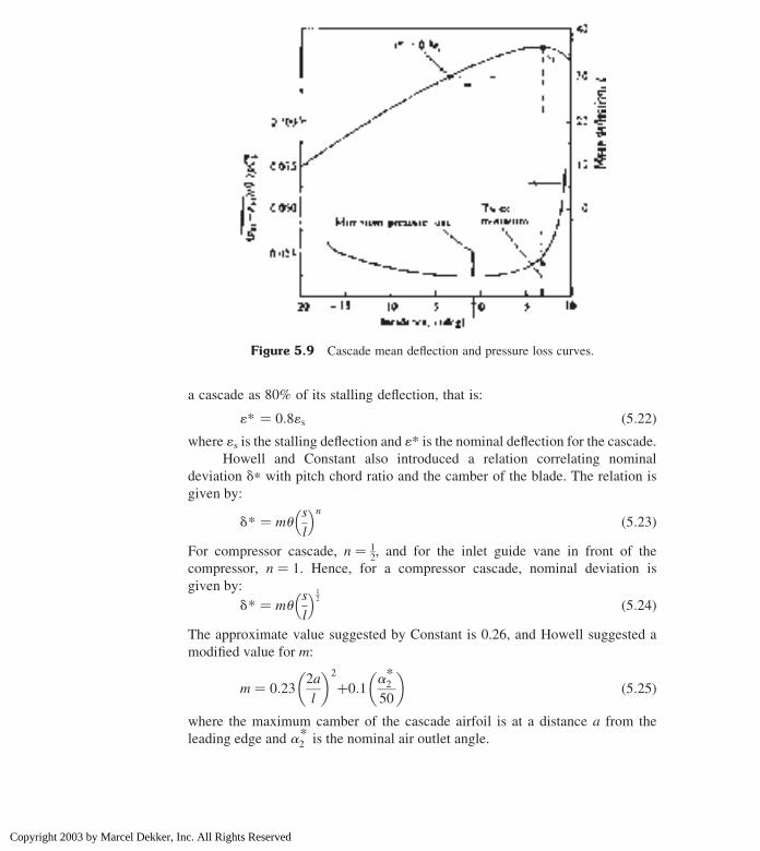
a cascade as 80% of its stalling deflection, that is:
1* ¼ 0:81s ð5:22Þwhere 1s is the stalling deflection and 1* is the nominal deflection for the cascade.
Howell and Constant also introduced a relation correlating nominal
deviation d* with pitch chord ratio and the camber of the blade. The relation is
given by:
d* ¼ mus
l
� �n ð5:23ÞFor compressor cascade, n ¼ 1
2, and for the inlet guide vane in front of the
compressor, n ¼ 1. Hence, for a compressor cascade, nominal deviation is
given by:
d* ¼ mus
l
� �12 ð5:24Þ
The approximate value suggested by Constant is 0.26, and Howell suggested a
modified value for m:
m ¼ 0:232a
l
� �2
þ0:1a*250
� �ð5:25Þ
where the maximum camber of the cascade airfoil is at a distance a from the
leading edge and a*2 is the nominal air outlet angle.
Figure 5.9 Cascade mean deflection and pressure loss curves.
Chapter 5198
Copyright 2003 by Marcel Dekker, Inc. All Rights Reserved
Then,
a*2 ¼ b2 þ d*
¼ b2 þ mus
l
� �12
and,
a*1 2 a*2 ¼ 1*
or:
a*1 ¼ a*2 þ 1*
Also,
i* ¼ a*1 2 b1 ¼ a*2 þ 1* 2 b1
5.7 3-D CONSIDERATION
So far, all the above discussions were based on the velocity triangle at one
particular radius of the blading. Actually, there is a considerable difference in
the velocity diagram between the blade hub and tip sections, as shown in
Fig. 5.10.
The shape of the velocity triangle will influence the blade geometry, and,
therefore, it is important to consider this in the design. In the case of a compressor
with high hub/tip ratio, there is little variation in blade speed from root to tip. The
shape of the velocity diagram does not change much and, therefore, little
variation in pressure occurs along the length of the blade. The blading is of the
same section at all radii and the performance of the compressor stage is calculated
from the performance of the blading at the mean radial section. The flow along
the compressor is considered to be 2-D. That is, in 2-D flow only whirl and axial
flow velocities exist with no radial velocity component. In an axial flow
compressor in which high hub/tip radius ratio exists on the order of 0.8, 2-D flow
in the compressor annulus is a fairly reasonable assumption. For hub/tip ratios
lower than 0.8, the assumption of two-dimensional flow is no longer valid. Such
compressors, having long blades relative to the mean diameter, have been used in
aircraft applications in which a high mass flow requires a large annulus area but a
small blade tip must be used to keep down the frontal area. Whenever the fluid
has an angular velocity as well as velocity in the direction parallel to the axis of
rotation, it is said to have “vorticity.” The flow through an axial compressor is
vortex flow in nature. The rotating fluid is subjected to a centrifugal force and to
balance this force, a radial pressure gradient is necessary. Let us consider
the pressure forces on a fluid element as shown in Fig. 5.10. Now, resolve
Axial Flow Compressors and Fans 199
Copyright 2003 by Marcel Dekker, Inc. All Rights Reserved

the forces in the radial direction Fig. 5.11:
du ðPþ dPÞðr þ drÞ2 Pr du2 2 Pþ dP
2
� �dr
du
2
¼ r dr r duC2w
rð5:26Þ
or
ðPþ dPÞðr þ drÞ2 Pr 2 Pþ dP
2
� �dr ¼ r dr C2
w
where: P is the pressure, r, the density, Cw, the whirl velocity, r, the radius.
After simplification, we get the following expression:
Pr þ P dr þ r dPþ dP dr 2 Pr þ r dr 21
2dP dr ¼ r dr C2
w
or:
r dP ¼ r dr C2w
Figure 5.10 Variation of velocity diagram along blade.
Chapter 5200
Copyright 2003 by Marcel Dekker, Inc. All Rights Reserved

That is,
1
r
dP
dr¼ C2
w
rð5:27Þ
The approximation represented by Eq. (5.27) has become known as radial
equilibrium.
The stagnation enthalpy h0 at any radius r where the absolute velocity is C
may be rewritten as:
h0 ¼ hþ 1
2C2a þ
1
2C2w; h ¼ cpT ; and C 2 ¼ C2
a þ C2w
� �
Differentiating the above equation w.r.t. r and equating it to zero yields:
dh0
dr¼ g
g2 1£ 1
r
dP
drþ 1
20þ 2Cw
dCw
dr
� �
Figure 5.11 Pressure forces on a fluid element.
Axial Flow Compressors and Fans 201
Copyright 2003 by Marcel Dekker, Inc. All Rights Reserved
or:
g
g2 1£ 1
r
dP
drþ Cw
dCw
dr¼ 0
Combining this with Eq. (5.27):
g
g2 1
C2w
rþ Cw
dCw
dr¼ 0
or:
dCw
dr¼ 2
g
g2 1
Cw
r
Separating the variables,
dCw
Cw
¼ 2g
g2 1
dr
r
Integrating the above equation
R dCw
Cw
¼ 2g
g2 1
Zdr
r
2g
g2 1lnCwr ¼ c where c is a constant:
Taking antilog on both sides,
g
g2 1£ Cw £ r ¼ e c
Therefore, we have
Cwr ¼ constant ð5:28ÞEquation (5.28) indicates that the whirl velocity component of the flow varies
inversely with the radius. This is commonly known as free vortex. The outlet
blade angles would therefore be calculated using the free vortex distribution.
5.8 MULTI-STAGE PERFORMANCE
An axial flow compressor consists of a number of stages. If R is the overall
pressure ratio, Rs is the stage pressure ratio, and N is the number of stages, then
the total pressure ratio is given by:
R ¼ ðRsÞN ð5:29ÞEquation (5.29) gives only a rough value of R because as the air passes
through the compressor the temperature rises continuously. The equation used to
Chapter 5202
Copyright 2003 by Marcel Dekker, Inc. All Rights Reserved

find stage pressure is given by:
Rs ¼ 1þ hsDT0s
T01
� � gg21
ð5:30Þ
The above equation indicates that the stage pressure ratio depends only on inlet
stagnation temperature T01, which goes on increasing in the successive stages. To
find the value of R, the concept of polytropic or small stage efficiency is very
useful. The polytropic or small stage efficiency of a compressor is given by:
h1;c ¼ g2 1
g
� �n
n2 1
� �
or:
n
n2 1
� �¼ hs
g
g2 1
� �
where hs ¼ h1,c ¼ small stage efficiency.
The overall pressure ratio is given by:
R ¼ 1þ NDT0s
T01
� � nn21
ð5:31Þ
Although Eq. (5.31) is used to find the overall pressure ratio of a
compressor, in actual practice the step-by-step method is used.
5.9 AXIAL FLOW COMPRESSORCHARACTERISTICS
The forms of characteristic curves of axial flow compressors are shown in
Fig. 5.12. These curves are quite similar to the centrifugal compressor.
However, axial flow compressors cover a narrower range of mass flow than the
centrifugal compressors, and the surge line is also steeper than that of a
centrifugal compressor. Surging and choking limit the curves at the two ends.
However, the surge points in the axial flow compressors are reached before the
curves reach a maximum value. In practice, the design points is very close to the
surge line. Therefore, the operating range of axial flow compressors is quite
narrow.
Illustrative Example 5.1: In an axial flow compressor air enters the
compressor at stagnation pressure and temperature of 1 bar and 292K,
respectively. The pressure ratio of the compressor is 9.5. If isentropic efficiency
of the compressor is 0.85, find the work of compression and the final temperature
at the outlet. Assume g ¼ 1.4, and Cp ¼ 1.005 kJ/kgK.
Axial Flow Compressors and Fans 203
Copyright 2003 by Marcel Dekker, Inc. All Rights Reserved

Solution:
T01 ¼ 292K; P01 ¼ 1 bar; hc ¼ 0:85:
Using the isentropic P–T relation for compression processes,
P02
P01
¼ T002
T01
� � gg21
where T02
0 is the isentropic temperature at the outlet.
Therefore,
T002 ¼ T01
P02
P01
� �g21g
¼ 292ð9:5Þ0:286 ¼ 555:92K
Now, using isentropic efficiency of the compressor in order to find the
actual temperature at the outlet,
T02 ¼ T01 þ T002 2 T01
� �
hc
¼ 292þ 555:922 292ð Þ0:85
¼ 602:49K
Figure 5.12 Axial flow compressor characteristics.
Chapter 5204
Copyright 2003 by Marcel Dekker, Inc. All Rights Reserved

Work of compression:
Wc ¼ CpðT02 2 T01Þ ¼ 1:005ð602:492 292Þ ¼ 312 kJ/kg
Illustrative Example 5.2: In one stage of an axial flow compressor, the
pressure ratio is to be 1.22 and the air inlet stagnation temperature is 288K. If the
stagnation temperature rise of the stages is 21K, the rotor tip speed is 200m/s, and
the rotor rotates at 4500 rpm, calculate the stage efficiency and diameter of the
rotor.
Solution:
The stage pressure ratio is given by:
Rs ¼ 1þ hsDT0s
T01
� � gg21
or
1:22 ¼ 1þ hsð21Þ288
� �3:5
that is,
hs ¼ 0:8026 or 80:26%
The rotor speed is given by:
U ¼ pDN
60; or D ¼ ð60Þð200Þ
pð4500Þ ¼ 0:85 m
Illustrative Example 5.3: An axial flow compressor has a tip diameter of
0.95m and a hub diameter of 0.85m. The absolute velocity of air makes an angle
of 288 measured from the axial direction and relative velocity angle is 568. Theabsolute velocity outlet angle is 568 and the relative velocity outlet angle is 288.The rotor rotates at 5000 rpm and the density of air is 1.2 kg/m3. Determine:
1. The axial velocity.
2. The mass flow rate.
3. The power required.
4. The flow angles at the hub.
5. The degree of reaction at the hub.
Solution:
1. Rotor speed is given by:
U ¼ pDN
60¼ pð0:95Þð5000Þ
60¼ 249m/s
Axial Flow Compressors and Fans 205
Copyright 2003 by Marcel Dekker, Inc. All Rights Reserved

Blade speed at the hub:
Uh ¼ pDhN
60¼ pð0:85Þð5000Þ
60¼ 223m/s
From the inlet velocity triangle (Fig. 5.13),
tana1 ¼ Cw1
Ca
and tanb1 ¼ U 2 Cw1ð ÞCa
Adding the above two equations:
U
Ca
¼ tana1 þ tanb1
or:
U ¼ Caðtan 288þ tan 568Þ ¼ Cað2:0146ÞTherefore, Ca ¼ 123.6m/s (constant at all radii)
2. The mass flow rate:
_m ¼ pðr2t 2 r2hÞrCa
¼ pð0:4752 2 0:4252Þð1:2Þð123:6Þ ¼ 20:98 kg/s
3. The power required per unit kg for compression is:
Wc ¼ lUCaðtanb1 2 tanb2Þ¼ ð1Þð249Þð123:6Þðtan 568 2 tan 288Þ1023
¼ ð249Þð123:6Þð1:4832 0:53Þ¼ 29:268 kJ/kg
Figure 5.13 Inlet velocity triangle.
Chapter 5206
Copyright 2003 by Marcel Dekker, Inc. All Rights Reserved

The total power required to drive the compressor is:
Wc ¼ _mð29:268Þ ¼ ð20:98Þð29:268Þ ¼ 614 kW
4. At the inlet to the rotor tip:
Cw1 ¼ Ca tana1 ¼ 123:6 tan 288 ¼ 65:72m/s
Using free vortex condition, i.e., Cwr ¼ constant, and using h as the
subscript for the hub,
Cw1h ¼ Cw1t
rt
rh¼ ð65:72Þ 0:475
0:425¼ 73:452m/s
At the outlet to the rotor tip,
Cw2t ¼ Catana2 ¼ 123:6 tan 568 ¼ 183:24m/s
Therefore,
Cw2h ¼ Cw2t
rt
rh¼ ð183:24Þ 0:475
0:425¼ 204:8m/s
Hence the flow angles at the hub:
tana1 ¼ Cw1h
Ca
¼ 73:452
123:6¼ 0:594 or; a1 ¼ 30:728
tanb1 ¼ Uhð ÞCa
2 tana1 ¼ 223
123:62 0:5942 ¼ 1:21
i.e., b1 ¼ 50.438
tana2 ¼ Cw2h
Ca
¼ 204:8
123:6¼ 1:657
i.e., a2 ¼ 58.898
tanb2 ¼ Uhð ÞCa
2 tana2 ¼ 223
123:62 tan 58:598 ¼ 0:1472
i.e., b2 ¼ 8.3785. The degree of reaction at the hub is given by:
Lh ¼ Ca
2Uh
ðtanb1 þ tanb2Þ ¼ 123:6
ð2Þð223Þ ðtan 50:438þ tan 8:378Þ
¼ 123:6
ð2Þð223Þ ð1:21þ 0:147Þ ¼ 37:61%
Axial Flow Compressors and Fans 207
Copyright 2003 by Marcel Dekker, Inc. All Rights Reserved

Illustrative Example 5.4: An axial flow compressor has the following
data:
Blade velocity at root: 140m/s
Blade velocity at mean radius: 185m/s
Blade velocity at tip: 240m/s
Stagnation temperature rise in this stage: 15K
Axial velocity ðconstant from root to tipÞ: 140m/s
Work done factor: 0:85
Degree of reaction at mean radius: 50%
Calculate the stage air angles at the root, mean, and tip for a free vortex
design.
Solution:
Calculation at mean radius:
From Eq. (5.1), Wc ¼ U(Cw2 2Cw1) ¼ UKCw
or:
CpðT02 2 T01Þ ¼ CpDT0s ¼ lUDCw
So:
DCw ¼ CpDT0s
lU¼ ð1005Þð15Þ
ð0:85Þð185Þ ¼ 95:87m/s
Since the degree of reaction (Fig. 5.14) at the mean radius is 50%, a1 ¼ b2
and a2 ¼ b1.
From the velocity triangle at the mean,
U ¼ DCw þ 2Cw1
or:
Cw1 ¼ U 2 DCw
2¼ 1852 95:87
2¼ 44:57m/s
Hence,
tana1 ¼ Cw1
Ca
¼ 44:57
140¼ 0:3184
that is,
a1 ¼ 17:668 ¼ b2
Chapter 5208
Copyright 2003 by Marcel Dekker, Inc. All Rights Reserved

and
tanb1 ¼ DCw þ Cw1ð ÞCa
¼ 95:87þ 44:57ð Þ140
¼ 1:003
i.e., b1 ¼ 45:098 ¼ a2
Calculation at the blade tip:
Using the free vortex diagram (Fig. 5.15),
ðDCw £ UÞt ¼ ðDCw £ UÞmTherefore,
DCw ¼ ð95:87Þð185Þ240
¼ 73:9m/s
Whirl velocity component at the tip:
Cw1 £ 240 ¼ ð44:57Þð185ÞTherefore:
Cw1 ¼ ð44:57Þð185Þ240
¼ 34:36m/s
tana1 ¼ Cw1
Ca
¼ 34:36
140¼ 0:245
Figure 5.14 Velocity triangle at the mean radius.
Axial Flow Compressors and Fans 209
Copyright 2003 by Marcel Dekker, Inc. All Rights Reserved

Therefore,
a1 ¼ 13:798
From the velocity triangle at the tip,
x2 þ DCw þ Cw1 ¼ U
or:
x2 ¼ U 2 DCw 2 Cw1 ¼ 2402 73:92 34:36 ¼ 131:74
tanb1 ¼ DCw þ x2
Ca
¼ 73:9þ 131:74
140¼ 1:469
i.e., b1 ¼ 55.758
tana2 ¼ Cw1 þ DCwð ÞCa
¼ 34:36þ 73:9ð Þ140
¼ 0:7733
i.e., a2 ¼ 37.718
tanb2 ¼ x2
Ca
¼ 131:74
140¼ 0:941
i.e., b2 ¼ 43.268
Calculation at the blade root:
ðDCw £ UÞr ¼ ðDCw £ UÞm
Figure 5.15 Velocity triangles at tip.
Chapter 5210
Copyright 2003 by Marcel Dekker, Inc. All Rights Reserved

or:
DCw £ 140 ¼ ð95:87Þð185Þ and DCw ¼ 126:69m/s
Also:
ðCw1 £ UÞr ¼ ðCw1 £ UÞmor:
Cw1 £ 140 ¼ ð44:57Þð185Þ and Cw1 ¼ 58:9m/s
and
ðCw2 £ UÞt ¼ ðCw2 £ UÞrso:
Cw2;tip ¼ Catana2 ¼ 140 tan 37:718 ¼ 108:24m/s
Therefore:
Cw2;root ¼ ð108:24Þð240Þ140
¼ 185:55m/s
tana1 ¼ 58:9
140¼ 0:421
i.e., a1 ¼ 22.828
From the velocity triangle at the blade root, (Fig. 5.16)
or:
x2 ¼ Cw2 2 U ¼ 185:552 140 ¼ 45:55
Figure 5.16 Velocity triangles at root.
Axial Flow Compressors and Fans 211
Copyright 2003 by Marcel Dekker, Inc. All Rights Reserved

Therefore:
tanb1 ¼ U 2 Cw1
Ca
¼ 1402 58:9
140¼ 0:579
i.e., b1 ¼ 30.088
tana2 ¼ Cw2
Ca
¼ 185:55
140¼ 1:325
i.e., a2 ¼ 52.968
tanb2 ¼ 2x2
Ca
¼ 245:55
140¼ 20:325
i.e., b2 ¼ 2188
Design Example 5.5: From the data given in the previous problem,
calculate the degree of reaction at the blade root and tip.
Solution:
Reaction at the blade root:
Lroot ¼ Ca
2Ur
ðtanb1rþ tanb2rÞ ¼ 140
ð2Þð140Þðtan30:088þ tan ð2188ÞÞ
¼ 140
ð2Þð140Þð0:57920:325Þ ¼ 0:127; or 12:7%
Reaction at the blade tip:
Ltip ¼ Ca
2Ut
ðtanb1t þ tanb2tÞ ¼ 140
ð2Þð240Þ ðtan55:758 þ tan43:268Þ
¼ 140
ð2Þð240Þ ð1:469þ 0:941Þ ¼ 0:7029; or 70:29%
Illustrative Example 5.6: An axial flow compressor stage has the
following data:
Air inlet stagnation temperature: 295K
Blade angle at outlet measured from the axial direction: 328
Flow coefficient: 0:56
Relative inlet Mach number: 0:78
Degree of reaction: 0:5
Find the stagnation temperature rise in the first stage of the compressor.
Chapter 5212
Copyright 2003 by Marcel Dekker, Inc. All Rights Reserved

Solution:
Since the degree of reaction is 50%, the velocity triangle is symmetric as
shown in Fig. 5.17. Using the degree of reaction equation [Eq. (5.12)]:
L ¼ Ca
2Uðtanb1 þ tanb2Þ and w ¼ Ca
U¼ 0:56
Therefore:
tanb1 ¼ 2L
0:562 tan 328 ¼ 1:16
i.e., b1 ¼ 49.248
Now, for the relative Mach number at the inlet:
Mr1 ¼ V1
gRT1
� �12
or:
V21 ¼ gRM2
r1 T01 2C21
2Cp
� �
From the velocity triangle,
V1 ¼ Ca
cosb1
; and C1 ¼ Ca
cosa1
and:
a1 ¼ b2ðsinceL ¼ 0:5ÞTherefore:
C1 ¼ Ca
cos328¼ Ca
0:848
Figure 5.17 Combined velocity triangles for Example 5.6.
Axial Flow Compressors and Fans 213
Copyright 2003 by Marcel Dekker, Inc. All Rights Reserved

and:
V1 ¼ Ca
cos 49:248¼ Ca
0:653
Hence:
C21 ¼
C2a
0:719; and V2
1 ¼C2a
0:426
Substituting for V1 and C1,
C2a ¼ 104:41 2952
C2a
1445
� �; so : Ca ¼ 169:51m/s
The stagnation temperature rise may be calculated as:
T02 2 T01 ¼ C2a
Cpwðtanb1 2 tanb2Þ
¼ 169:512
ð1005Þð0:56Þ ðtan 49:248 2 tan 328Þ ¼ 27:31K
Design Example 5.7: An axial flow compressor has the following
design data:
Inlet stagnation temperature: 290K
Inlet stagnation pressure: 1 bar
Stage stagnation temperature rise: 24K
Mass flow of air: 22kg/s
Axialvelocity through the stage: 155:5m/s
Rotational speed: 152rev/s
Work done factor: 0:93
Mean blade speed: 205m/s
Reaction at the mean radius: 50%
Determine: (1) the blade and air angles at the mean radius, (2) the mean
radius, and (3) the blade height.
Chapter 5214
Copyright 2003 by Marcel Dekker, Inc. All Rights Reserved
Solution:
(1) The following equation provides the relationship between the
temperature rise and the desired angles:
T02 2 T01 ¼ lUCa
Cp
ðtanb1 2 tanb2Þor:
24 ¼ ð0:93Þð205Þð155:5Þ1005
ðtanb1 2 tanb2Þso:
tanb1 2 tanb2 ¼ 0:814
Using the degree of reaction equation:
L ¼ Ca
2Uðtanb1 þ tanb2Þ
Hence:
tanb1 þ tanb2 ¼ ð0:5Þð2Þð205Þ155:5
¼ 1:318
Solving the above two equations simultaneously for b1 and b2,
2 tanb1 ¼ 2:132;
so : b1 ¼ 46:838 ¼ a2 ðsince the degree of reaction is 50%Þand:
tanb2 ¼ 1:3182 tan 46:838 ¼ 1:3182 1:066;
so : b2 ¼ 14:148 ¼ a1
(2) The mean radius, rm, is given by:
rm ¼ U
2pN¼ 205
ð2pÞð152Þ ¼ 0:215m
(3) The blade height, h, is given by:
m ¼ rACa, where A is the annular area of the flow.
C1 ¼ Ca
cosa1
¼ 155:5
cos14:148¼ 160:31m/s
T1 ¼ T01 2C21
2Cp
¼ 2902160:312
ð2Þð1005Þ ¼ 277:21K
Axial Flow Compressors and Fans 215
Copyright 2003 by Marcel Dekker, Inc. All Rights Reserved

Using the isentropic P–T relation:
P1
P01
¼ T1
T01
� � gg21
Static pressure:
P1 ¼ ð1Þ 277:21
290
� �3:5¼ 0:854 bar
Then:
r1 ¼ P1
RT1
¼ ð0:854Þð100Þð0:287Þð277:21Þ ¼ 1:073 kg/m3
From the continuity equation:
A ¼ 22
ð1:073Þð155:5Þ ¼ 0:132m2
and the blade height:
h ¼ A
2prm¼ 0:132
ð2pÞð0:215Þ ¼ 0:098m
Illustrative Example 5.8: An axial flow compressor has an overall
pressure ratio of 4.5:1, and a mean blade speed of 245m/s. Each stage is of 50%
reaction and the relative air angles are the same (308) for each stage. The axial
velocity is 158m/s and is constant through the stage. If the polytropic efficiency
is 87%, calculate the number of stages required. Assume T01 ¼ 290K.
Solution:
Since the degree of reaction at the mean radius is 50%, a1 ¼ b2 and
a2 ¼ b1. From the velocity triangles, the relative outlet velocity component
in the x-direction is given by:
Vx2 ¼ Catanb2 ¼ 158tan 308 ¼ 91:22m/s
V1 ¼ C2 ¼ ðU 2 Vx2Þ2 þ C2a
12
¼ ð2452 91:22Þ2 þ 1582 1
2¼ 220:48m/s
cos b1 ¼ Ca
V1
¼ 158
220:48¼ 0:7166
so: b1 ¼ 44.238
Chapter 5216
Copyright 2003 by Marcel Dekker, Inc. All Rights Reserved

Stagnation temperature rise in the stage,
DT0s ¼ UCa
Cp
ðtanb1 2 tanb2Þ
¼ ð245Þð158Þ1005
ðtan 44:238 2 tan 308Þ ¼ 15:21K
Number of stages
R ¼ 1þ NDT0s
T01
� � nn21
n
n2 1¼ h1
g
g2 1¼ 0:87
1:4
0:4¼ 3:05
Substituting:
4:5 ¼ 1þ N15:21
290
� �3:05
Therefore,
N ¼ 12 stages:
Design Example 5.9: In an axial flow compressor, air enters at a stagnation
temperature of 290K and 1 bar. The axial velocity of air is 180m/s (constant
throughout the stage), the absolute velocity at the inlet is 185m/s, the work done
factor is 0.86, and the degree of reaction is 50%. If the stage efficiency is 0.86,
calculate the air angles at the rotor inlet and outlet and the static temperature at
the inlet of the first stage and stage pressure ratio. Assume a rotor speed of
200m/s.
Solution:
For 50% degree of reaction at the mean radius (Fig. 5.18), a1 ¼ b2 and
a2 ¼ b1.
From the inlet velocity triangle,
cos a1 ¼ Ca
C1
¼ 180
185¼ 0:973
i.e., a1 ¼ 13.358 ¼ b2
From the same velocity triangle,
Cw1 ¼ C21 2 C2
a
� �12 ¼ 1852 2 1802
� �12 ¼ 42:72m/s
Axial Flow Compressors and Fans 217
Copyright 2003 by Marcel Dekker, Inc. All Rights Reserved
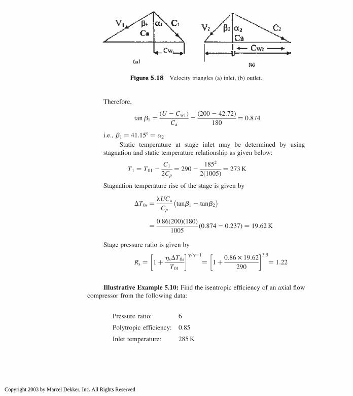
Therefore,
tanb1 ¼ U 2 Cw1ð ÞCa
¼ 2002 42:72ð Þ180
¼ 0:874
i.e., b1 ¼ 41.158 ¼ a2
Static temperature at stage inlet may be determined by using
stagnation and static temperature relationship as given below:
T1 ¼ T01 2C1
2Cp
¼ 29021852
2ð1005Þ ¼ 273K
Stagnation temperature rise of the stage is given by
DT0s ¼ lUCa
Cp
tanb1 2 tanb2
� �
¼ 0:86ð200Þð180Þ1005
0:8742 0:237ð Þ ¼ 19:62K
Stage pressure ratio is given by
Rs ¼ 1þ hsDT0s
T01
� �g=g21
¼ 1þ 0:86 £ 19:62
290
� �3:5¼ 1:22
Illustrative Example 5.10: Find the isentropic efficiency of an axial flow
compressor from the following data:
Pressure ratio: 6
Polytropic efficiency: 0:85
Inlet temperature: 285K
Figure 5.18 Velocity triangles (a) inlet, (b) outlet.
Chapter 5218
Copyright 2003 by Marcel Dekker, Inc. All Rights Reserved

Solution:
Using the isentropic P–T relation for the compression process,
T020 ¼ T01
P02
P01
� �g21g
¼ 285 6ð Þ0:286¼ 475:77K
Using the polytropic P–T relation for the compression process:
n2 1
n¼ g2 1
gh1;c¼ 0:4
1:4ð0:85Þ ¼ 0:336
Actual temperature rise:
T02 ¼ T01
p02
p01
� �ðn21Þ=n¼ 285 6ð Þ0:336¼ 520:36K
The compressor isentropic efficiency is given by:
hc ¼ T020 2 T01
T02 2 T01
¼ 475:772 285
5202 285¼ 0:8105; or 81:05%
Design Example 5.11: In an axial flow compressor air enters the
compressor at 1 bar and 290K. The first stage of the compressor is designed on
free vortex principles, with no inlet guide vanes. The rotational speed is 5500 rpm
and stagnation temperature rise is 22K. The hub tip ratio is 0.5, the work done
factor is 0.92, and the isentropic efficiency of the stage is 0.90. Assuming an inlet
velocity of 145m/s, calculate
1. The tip radius and corresponding rotor air angles, if the Mach number
relative to the tip is limited to 0.96.
2. The mass flow at compressor inlet.
3. The stagnation pressure ratio and power required to drive the
compressor.
4. The rotor air angles at the root section.
Solution:
(1) As no inlet guide vanes
a1 ¼ 0;Cw1 ¼ 0
Stagnation temperature, T01, is given by
T01 ¼ T1 þ C1
2Cp2
or
T1 ¼ T01 2C1
2Cp
¼ 29021452
2 £ 1005¼ 288:9K
Axial Flow Compressors and Fans 219
Copyright 2003 by Marcel Dekker, Inc. All Rights Reserved

The Mach number relative to tip is
M ¼ V1ffiffiffiffiffiffiffiffiffiffiffigRT1
p
or
V1 ¼ 0:96 1:4 £ 287 £ 288:9ð Þ0:5¼ 340:7m/s
i.e., relative velocity at tip ¼ 340.7m/s
From velocity triangle at inlet (Fig. 5.3)
V21 ¼ U2
t þ C21 orUt ¼ 340:72 2 1452
� �0:5¼ 308:3m/s
or tip speed,
Ut ¼ 2prtN
60
or
rt ¼ 308:3 £ 60
2p £ 5500¼ 0:535m:
tanb1 ¼ Ut
Ca
¼ 308:3
145¼ 2:126
i:e:; b1 ¼ 64:818
Stagnation temperature rise
DT0s ¼ tUCa
Cp
tanb1 2 tanb2
� �
Substituting the values, we get
22 ¼ 0:92 £ 308:3 £ 145
1005tanb1 2 tanb2
� �
or
tanb1 2 tanb2
� � ¼ 0:538
(2) Therefore, tanb2 ¼ 1.588 and b2 ¼ 57.88
root radius/tip radius ¼ rm 2 h/2
rm þ h/2¼ 0:5
(where subscript m for mean and h for height)
or rm 2 h/2 ¼ 0.5 rm þ 0.25 h
[ rm ¼ 1.5 h
but rt ¼ rm þ h/2 ¼ 1.5 h þ h/2
Chapter 5220
Copyright 2003 by Marcel Dekker, Inc. All Rights Reserved

or 0.535 ¼ 2 h or h ¼ 0.268m
and rm ¼ 1.5 h ¼ 0.402m
Area, A ¼ 2prmh ¼ 2p £ 0.402 £ 0.268 ¼ 0.677m2
Now, using isentropic relationship for p–T
p1
p01¼ T1
T01
� �g/ g21ð Þor p1 ¼ 1 £ 288:9
290
� �3:5¼ 0:987 bar
and
r1 ¼ p1
RT1
¼ 0:987 £ 105
287 £ 288:9¼ 1:19 kg/m3
Therefore, the mass flow entering the stage
_m ¼ rACa ¼ 1:19 £ 0:677 £ 145 ¼ 116:8 kg/s
(3) Stage pressure ratio is
Rs ¼ 1þ hsDT0s
T01
� �g/ g21ð Þ
¼ 1þ 0:90 £ 22
290
� �3:5¼ 1:26
Now,
W ¼ CpDT0s ¼ 1005 £ 22 ¼ 22110J/kg
Power required by the compressor
P ¼ _mW ¼ 116:8 £ 22110 ¼ 2582:4 kW
(4) In order to find out rotor air angles at the root section, radius at the
root can be found as given below.
rr ¼ rm 2 h/2
¼ 0:4022 0:268/2 ¼ 0:267m:
Impeller speed at root is
Ur ¼ 2prrN
60
¼ 2 £ p £ 0:267 £ 5500
60¼ 153:843m/s
Axial Flow Compressors and Fans 221
Copyright 2003 by Marcel Dekker, Inc. All Rights Reserved

Therefore, from velocity triangle at root section
tanb1 ¼ Ur
Ca
¼ 153:843
145¼ 1:061
i:e:; b1 ¼ 46:98
For b2 at the root section
DT0s ¼ tUrCa
Cp
tanb1 2 tanb2
� �
or
22 ¼ 0:92 £ 153:843 £ 145
1005tanb1 2 tanb2
� �
or
tanb1 2 tanb2
� � ¼ 1:078
[ b2 ¼ 20:9748
Design Example 5.12: The following design data apply to an axial flow
compressor:
Overall pressure ratio: 4:5
Mass flow: 3:5kg/s
Polytropic efficiency: 0:87
Stagnation temperature rise per stage: 22k
Absolute velocity approaching the last rotor: 160m/s
Absolute velocity angle; measured from the axial direction: 208
Work done factor: 0:85
Mean diameter of the last stage rotor is: 18:5cm
Ambient pressure: 1:0bar
Ambient temperature: 290K
Calculate the number of stages required, pressure ratio of the first and last
stages, rotational speed, and the length of the last stage rotor blade at inlet to the
stage. Assume equal temperature rise in all stages, and symmetrical velocity
diagram.
Chapter 5222
Copyright 2003 by Marcel Dekker, Inc. All Rights Reserved

Solution:
If N is the number of stages, then overall pressure rise is:
R ¼ 1þ NDT0s
T01
� �n21n
where
n2 1
n¼ hac
g
g2 1
(where hac is the polytropic efficiency)
substituting values
n2 1
n¼ 0:87 £ 1:4
0:4¼ 3:05
overall pressure ratio, R is
R ¼ 1þ N £ 22
290
� �3:05
or
4:5ð Þ 13:05 ¼ 1þ N £ 22
290
� �
[ N ¼ 8:4
Hence number of stages ¼ 8
Stagnation temperature rise, DT0s, per stage ¼ 22K, as we took 8
stages, therefore
DT0s ¼ 22 £ 8:4
8¼ 23:1
From velocity triangle
cos a8 ¼ Ca8
C8
or
Ca8 ¼ 160 £ cos20 ¼ 150:35m/s
Using degree of reaction, L ¼ 0.5
Then,
0:5 ¼ Ca8
2Utanb8 þ tanb9
� �
Axial Flow Compressors and Fans 223
Copyright 2003 by Marcel Dekker, Inc. All Rights Reserved

or
0:5 ¼ 150:35
2Utanb8 þ tanb9
� � ðAÞAlso,
DT0s ¼ tUCa8
Cp
tanb8 2 tanb9
� �
Now, DT0s ¼ 22K for one stage.
As we took 8 stages, therefore;
DT0s ¼ 22 £ 8:4
8¼ 23:1K
[ 23:1 ¼ 0:85 £ U £ 150:35
1005tanb8 2 tan20� � ðBÞ
Because of symmetry, a8 ¼ b9 ¼ 208From Eq. (A)
U ¼ 150:35 tanb8 þ 0:364� � ðCÞ
From Eq. (B)
U ¼ 181:66
tanb8 2 0:364ðDÞ
Comparing Eqs. (C) and (D), we have
150:35 tanb8 þ 0:364� � ¼ 181:66
tanb8 2 0:364� �
or
tan 2b8 2 0:3642� � ¼ 181:66
150:35¼ 1:21
or
tan2b8 ¼ 1:21þ 0:1325 ¼ 1:342
[ tanb8 ¼ffiffiffiffiffiffiffiffiffiffiffi1:342
p ¼ 1:159
i:e:;b8 ¼ 49:208
Substituting in Eq. (C)
U ¼ 150:35 tan 49:208þ 0:364ð Þ¼ 228:9m/s
Chapter 5224
Copyright 2003 by Marcel Dekker, Inc. All Rights Reserved

The rotational speed is given by
N ¼ 228:9
2p £ 0:0925¼ 393:69rps
In order to find the length of the last stage rotor blade at inlet to the stage, it
is necessary to calculate stagnation temperature and pressure ratio of the
last stage.
Stagnation temperature of last stage: Fig. 5.19
To8 ¼ T01 þ 7 £ T0s
¼ 290þ 7 £ 23:1 ¼ 451:7K
Pressure ratio of the first stage is:
R ¼ 1þ 1 £ 23:1
451:7
� �3:05
Now,
p08/p09 ¼ 1:1643
p09
p01¼ 4; and p09 ¼ 4bar
p08 ¼ 4
1:1643¼ 3:44bar
and
T08 ¼ T8 þ C28
2Cp
or
T8 ¼ T08 2C28
2Cp
¼ 451:721602
2 £ 1005
¼ 438:96K
Figure 5.19 Velocity diagram of last stage.
Axial Flow Compressors and Fans 225
Copyright 2003 by Marcel Dekker, Inc. All Rights Reserved

Using stagnation and static isentropic temperature relationship for the last
stage, we have
p8
p08¼ T8
T08
� �1:4/0:4
Therefore,
p8 ¼ 3:44438:96
451:7
� �3:5
¼ 3:112bar
andr8 ¼ p8
RT8
¼ 3:112 £ 105
287 £ 438:9¼ 2:471 kg/m3
Using mass flow rate
_m ¼ r8A8Ca8
or
3:5 ¼ 2:471 £ A8 £ 150:35
[ A8 ¼ 0:0094m 2
¼ 2prhor
h ¼ 0:0094
2p £ 0:0925¼ 0:0162m
i.e., length of the last stage rotor blade at inlet to the stage,
h ¼ 16.17mm.
Design Example 5.13: A 10-stage axial flow compressor is designed for
stagnation pressure ratio of 4.5:1. The overall isentropic efficiency of the
compressor is 88% and stagnation temperature at inlet is 290K. Assume equal
temperature rise in all stages, and work done factor is 0.87. Determine the air
angles of a stage at the design radius where the blade speed is 218m/s. Assume a
constant axial velocity of 165m/s, and the degree of reaction is 76%.
Solution:
No. of stages ¼ 10
The overall stagnation temperature rise is:
T0 ¼T01 R
g21g 2 1
� �
hc
¼ 290 4:50:286 2 1� �
0:88
¼ 155:879K
Chapter 5226
Copyright 2003 by Marcel Dekker, Inc. All Rights Reserved

The stagnation temperature rise of a stage
T0s ¼ 155:879
10¼ 15:588K
The stagnation temperature rise in terms of air angles is:
T0s ¼ tUCa
Cp
tana2 2 tana1ð Þ
or
tana2 2 tana1ð Þ ¼ T0s £ Cp
tUCa
¼ 15:588 £ 1005
0:87 £ 218 £ 165
¼ 0:501 ðAÞ
From degree of reaction
^ ¼ 12Ca
2Utana2 þ tana1ð Þ
� �
or
0:76 ¼ 12165
2 £ 218tana2 þ tana1ð Þ
� �
[ tana2 þ tana1ð Þ ¼ 0:24 £ 2 £ 218
165¼ 0:634 ðBÞ
Adding (A) and (B), we get
2 tana2 ¼ 1.135
or tana2 ¼ 0.5675
i.e., a2 ¼ 29.578
and tana1 ¼ 0.634 2 0.5675 ¼ 0.0665
i.e., a1 ¼ 3.808
Similarly, for b1 and b2, degree of reaction
tanb1 þ tanb2 ¼ 2.01
and tanb1 2 tan b2 ¼ 0.501
[ 2 tanb1 ¼ 2.511
i.e., b1 ¼ 51.468
and tanb2 ¼ 1.1256 2 0.501 ¼ 0.755
i.e., b2 ¼ 37.038
Axial Flow Compressors and Fans 227
Copyright 2003 by Marcel Dekker, Inc. All Rights Reserved

Design Example 5.14: An axial flow compressor has a tip diameter of
0.9m, hub diameter of 0.42m, work done factor is 0.93, and runs at 5400 rpm.
Angles of absolute velocities at inlet and exit are 28 and 588, respectively and
velocity diagram is symmetrical. Assume air density of 1.5 kg/m3, calculate mass
flow rate, work absorbed by the compressor, flow angles and degree of reaction at
the hub for a free vortex design.
Solution:
Impeller speed is
U ¼ 2prN
60¼ 2p £ 0:45 £ 5400
60¼ 254:57m/s
From velocity triangle
U ¼ Ca tana1 þ tanb1
� �
Ca ¼ U
tana1 þ tanb1
¼ 254:57
tan 288þ tan 588ð Þ ¼ 119:47 m/s
Flow area is
A ¼ p rtip 2 rroot
¼ p 0:452 2 0:422 ¼ 0:0833m2
Mass flow rate is
_m ¼ rACa ¼ 1:5 £ 0:0833 £ 119:47 ¼ 14:928 kg/s
Power absorbed by the compressor
¼ tU Cw2 2 Cw1ð Þ¼ tUCa tana2 2 tana1ð Þ¼ 0:93 £ 254:57 £ 119:47 tan 588 2 tan 288ð Þ¼ 30213:7Nm
Total Power;P ¼_m £ 30213:7
1000kW
¼ 451 kW
and whirl velocity at impeller tip Cwt ¼ Ca tan a1 ¼ 119.47 £tan 288 ¼ 63.52m/s
Now using free vortex condition
r Cw ¼ constant
[ rhCw1h ¼ rtCw1t (where subscripts h for hub and t for tip)
Chapter 5228
Copyright 2003 by Marcel Dekker, Inc. All Rights Reserved

or
Cw1h ¼ rtCw1t
rh¼ 0:45 £ 63:52
0:4¼ 71:46m/s
Similarly
Cw2t ¼ Ca tana2 ¼ 119:47 tan588 ¼ 191:2m/s
and
rhCw2h ¼ rtCw2t
or
Cw2h ¼ rtCw2t
rh¼ 0:45 £ 191:2
0:4¼ 215:09m/s
Therefore, the flow angles at the hub are
tana1 ¼ Cw1h
Ca
ðwhere Ca is constantÞ
¼ 71:46
119:47¼ 0:598
i.e., a1 ¼ 30.888
tanb1 ¼Uh 2 Catana1
Ca
where Uh at the hub is given by
Uh ¼ 2prhN ¼ 2 £ p £ 0:4 £ 5400
60¼ 226:29m/s
[ tanb1 ¼ 226:292 119:47 tan30:888
119:47
i.e., b1 ¼ 52.348
tana2 ¼ Cw2h
Ca
¼ 215:09
119:47¼ 1:80
i.e., a2 ¼ 60.958Similarly,
tanb2 ¼ Uh 2 Catana2
Ca
¼ 226:292 119:47 tan 60:958
119:47
i.e., b2 ¼ 5.368
Axial Flow Compressors and Fans 229
Copyright 2003 by Marcel Dekker, Inc. All Rights Reserved

Finally, the degree of reaction at the hub is
^ ¼ Ca
2Uh
tanb1 þ tanb2
� � ¼ 119:47
2 £ 226:29tan52:348þ tan5:368ð Þ
¼ 0:367 or 36:7%:
Design Example 5.15: An axial flow compressor is to deliver 22 kg of air per
second at a speed of 8000 rpm. The stagnation temperature rise of the first stage is
20K. The axial velocity is constant at 155m/s, and work done factor is 0.94. The
mean blade speed is 200m/s, and reaction at the mean radius is 50%. The rotor
blade aspect ratio is 3, inlet stagnation temperature and pressure are 290K and
1.0 bar, respectively. Assume Cp for air as 1005 J/kgK and g ¼ 1.4. Determine:
1. The blade and air angles at the mean radius.
2. The mean radius.
3. The blade height.
4. The pitch and chord.
Solution:
1. Using Eq. (5.10) at the mean radius
T02 2 T01 ¼ tUCa
Cp
tanb1 2 tanb2
� �
20 ¼ 0:94 £ 200 £ 155
1005tanb1 2 tanb2
� �
tanb1 2 tanb2
� � ¼ 0:6898
Using Eq. (5.12), the degree of reaction is
^ ¼ Ca
2Utanb1 þ tanb2
� �
or
tanb1 þ tanb2
� � ¼ 0:5 £ 2 £ 200
155¼ 1:29
Solving above two equations simultaneously
2 tanb1 ¼ 1:98
[ b1 ¼ 44:718 ¼ a2 ðas the diagram is symmetricalÞtanb2 ¼ 1:292 tan44:718
i.e.,
b2 ¼ 16:708 ¼ a1
Chapter 5230
Copyright 2003 by Marcel Dekker, Inc. All Rights Reserved

2. Let rm be the mean radius
rm ¼ U
2pN¼ 200 £ 60
2p £ 8000¼ 0:239m
3. Using continuity equation in order to find the annulus area of flow
C1 ¼ Ca
cosa1
¼ 155
cos16:708¼ 162m/s
T1 ¼ T01 2C21
2Cp
¼ 29021622
2 £ 1005¼ 276:94K
Using isentropic relationship at inlet
p1
p01¼ T1
T01
� � gg21
Static pressure is
p1 ¼ 1:0276:94
290
� �3:5
¼ 0:851bars
Density is
r1 ¼ p1
RT1
¼ 0:851 £ 100
0:287 £ 276:94¼ 1:07 kg/m3
From the continuity equation,
A ¼ 22
1:07 £ 155¼ 0:133m2
Blade height is
h ¼ A
2prm¼ 0:133
2 £ p £ 0:239¼ 0:089m:
4. At mean radius, and noting that blades b, an equivalent to cascade, a,nominal air deflection is
1 ¼ b1 2 b2
¼ 44:718 2 16:708 ¼ 28:018
Using Fig. 5.20 for cascade nominal deflection vs. air outlet angle, the
solidity,
s
c¼ 0:5
Blade aspect ratio ¼ span
chord
Axial Flow Compressors and Fans 231
Copyright 2003 by Marcel Dekker, Inc. All Rights Reserved

Blade chord,
C ¼ 0:089
3¼ 0:03m
Blade pitch,
s ¼ 0:5 £ 0:03 ¼ 0:015m:
PROBLEMS
5.1 An axial flow compressor has constant axial velocity throughout the
compressor of 152m/s, a mean blade speed of 162m/s, and delivers 10.5 kg
of air per second at a speed of 10,500 rpm. Each stage is of 50% reaction
and the work done factor is 0.92. If the static temperature and pressure at the
inlet to the first stage are 288K and 1 bar, respectively, and the stagnation
stage temperature rise is 15K, calculate: 1 the mean diameter of the blade
row, (2) the blade height, (3) the air exit angle from the rotating blades, and
(4) the stagnation pressure ratio of the stage with stage efficiency 0.84.
(0.295m, 0.062m, 11.378, 1.15)
5.2 The following design data apply to an axial flow compressor:
Stagnation temperature rise of the stage: 20K
Work done factor: 0:90
Blade velocity at root: 155m/s
Figure 5.20 Cascade nominal deflection versus air outlet angle.
Chapter 5232
Copyright 2003 by Marcel Dekker, Inc. All Rights Reserved

Blade velocity at mean radius: 208m/s
Blade velocity at tip: 255m/s
Axial velocity ðconstant through the stageÞ: 155m/s
Degree of reaction at mean radius: 0:5
Calculate the inlet and outlet air and blade angles at the root, mean radius
and tip for a free vortex design.
(188, 45.58, 14.848, 54.078, 39.718, 39.188, 23.568, 29.428, 53.758, 2208)
5.3 Calculate thedegreeofreactionat thetipandrootfor thesamedataasProb.5.2.
(66.7%, 10%)
5.4 Calculate the air and blade angles at the root, mean and tip for 50% degree
of reaction at all radii for the same data as in Prob. [5.2].
(47.868, 28.378, 43.988, 1.728)
5.5 Show that for vortex flow,
Cw £ r ¼ constant
that is, the whirl velocity component of the flow varies inversely with the
radius.
5.6 The inlet and outlet angles of an axial flow compressor rotor are 50 and 158,respectively. The blades are symmetrical; mean blade speed and axial
velocity remain constant throughout the compressor. If the mean blade
speed is 200m/s, work done factor is 0.86, pressure ratio is 4, inlet
stagnation temperature is equal to 290K, and polytropic efficiency of the
compressor is 0.85, find the number of stages required.
(8 stages)
5.7 In an axial flow compressor air enters at 1 bar and 158C. It is compressed
through a pressure ratio of four. Find the actual work of compression and
temperature at the outlet from the compressor. Take the isentropic
efficiency of the compressor to be equal to 0.84
. (167.66 kJ/kg, 454.83K)
5.8 Determine the number of stages required to drive the compressor for an
axial flow compressor having the following data: difference between the
tangents of the angles at outlet and inlet, i.e., tanb1 - tanb2 ¼ 0.55. The
isentropic efficiency of the stage is 0.84, the stagnation temperature at
the compressor inlet is 288K, stagnation pressure at compressor inlet is
1 bar, the overall stagnation pressure rise is 3.5 bar, and the mass flow rate is
15 kg/s. Assume Cp ¼ 1.005 kJ/kgK, g ¼ 1.4, l ¼ 0.86, hm ¼ 0.99
(10 stages, 287.5 kW)
Axial Flow Compressors and Fans 233
Copyright 2003 by Marcel Dekker, Inc. All Rights Reserved

5.9 From the data given below, calculate the power required to drive the
compressor and stage air angles for an axial flow compressor.
Stagnation temperature at the inlet: 288K
Overall pressure ratio: 4
Isentropic efficiency of the compressor: 0:88
Mean blade speed: 170m/s
Axial velocity: 120m/s
Degree of reaction: 0:5
(639.4 kW, b1 ¼ 77.88, b2 ¼ 272.698)
5.10 Calculate the number of stages from the data given below for an axial flow
compressor:
Air stagnation temperature at the inlet: 288K
Stage isentropic efficiency: 0:85
Degree of reaction: 0:5
Air angles at rotor inlet: 408
Air angle at the rotor outlet: 108
Meanblade speed: 180m/s
Work done factor: 0:85
Overall pressure ratio: 6
(14 stages)
5.11 Derive the expression for polytropic efficiency of an axial flow
compressor in terms of:
(a) n and g(b) inlet and exit stagnation temperatures and pressures.
5.12 Sketch the velocity diagrams for an axial flow compressor and derive the
expression:
P02
P01
¼ 1þ hsDT0s
T01
� � gg21
5.13 Explain the term “degree of reaction”. Why is the degree of reaction
generally kept at 50%?
5.14 Derive an expression for the degree of reaction and show that for 50%
reaction, the blades are symmetrical; i.e., a1 ¼ b2 and a2 ¼ b1.
5.16 What is vortex theory? Derive an expression for vortex flow.
5.17 What is an airfoil? Define, with a sketch, the various terms used in airfoil
geometry.
Chapter 5234
Copyright 2003 by Marcel Dekker, Inc. All Rights Reserved

NOTATION
C absolute velocity
CL lift coefficient
Cp specific heat at constant pressure
D drag
Fx tangential force on moving blade
h blade height, specific enthalpy
L lift
N number of stage, rpm
n number of blades
R overall pressure ratio, gas constant
Rs stage pressure ratio
U tangential velocity
V relative velocity
a angle with absolute velocity, measured from the axial direction
a*2 nominal air outlet angle
b angle with relative velocity, measure from the axial direction
DTA static temperature rise in the rotor
DTB static temperature rise in the stator
DT0s stagnation temperature rise
DTs static temperature rise
D* nominal deviation
e* nominal deflection
es stalling deflection
w flow coefficient
L degree of reaction
l work done factor
c stage loading factor
SUFFIXES
1 inlet to rotor
2 outlet from the rotor
3 inlet to second stage
a axial, ambient
m mean
r radial, root
t tip
w whirl
Axial Flow Compressors and Fans 235
Copyright 2003 by Marcel Dekker, Inc. All Rights Reserved


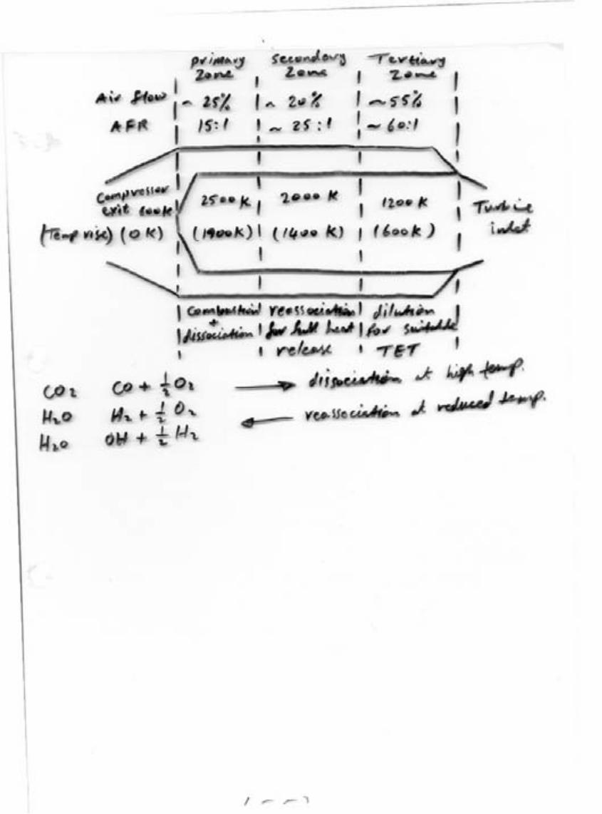


7
Axial Flow and Radial FlowGas Turbines
7.1 INTRODUCTION TO AXIAL FLOW TURBINES
The axial flow gas turbine is used in almost all applications of gas turbine power
plant. Development of the axial flow gas turbine was hindered by the need to
obtain both a high-enough flow rate and compression ratio from a compressor to
maintain the air requirement for the combustion process and subsequent
expansion of the exhaust gases. There are two basic types of turbines: the axial
flow type and the radial or centrifugal flow type. The axial flow type has been
used exclusively in aircraft gas turbine engines to date and will be discussed in
detail in this chapter. Axial flow turbines are also normally employed in industrial
and shipboard applications. Figure 7.1 shows a rotating assembly of the Rolls-
Royce Nene engine, showing a typical single-stage turbine installation. On this
particular engine, the single-stage turbine is directly connected to the main and
cooling compressors. The axial flow turbine consists of one or more stages
located immediately to the rear of the engine combustion chamber. The turbine
extracts kinetic energy from the expanding gases as the gases come from the
burner, converting this kinetic energy into shaft power to drive the compressor
and the engine accessories. The turbines can be classified as (1) impulse and
(2) reaction. In the impulse turbine, the gases will be expanded in the nozzle and
passed over to the moving blades. The moving blades convert this kinetic
energy into mechanical energy and also direct the gas flow to the next stage
Copyright 2003 by Marcel Dekker, Inc. All Rights Reserved

(multi-stage turbine) or to exit (single-stage turbine). Fig. 7.1 shows the axial
flow turbine rotors.
In the case of reaction turbine, pressure drop of expansion takes place in the
stator as well as in the rotor-blades. The blade passage area varies continuously to
allow for the continued expansion of the gas stream over the rotor-blades. The
efficiency of a well-designed turbine is higher than the efficiency of a
compressor, and the design process is often much simpler. The main reason for
this fact, as discussed in compressor design, is that the fluid undergoes a pressure
rise in the compressor. It is much more difficult to arrange for an efficient
deceleration of flow than it is to obtain an efficient acceleration. The pressure
drop in the turbine is sufficient to keep the boundary layer fluid well behaved, and
separation problems, or breakaway of the molecules from the surface, which
often can be serious in compressors, can be easily avoided. However, the turbine
designer will face much more critical stress problem because the turbine rotors
must operate in very high-temperature gases. Since the design principle and
concepts of gas turbines are essentially the same as steam turbines, additional
Figure 7.1 Axial flow turbine rotors. (Courtesy Rolls-Royce.)
Chapter 7284
Copyright 2003 by Marcel Dekker, Inc. All Rights Reserved

information on turbines in general already discussed in Chapter 6 on steam
turbines.
7.2 VELOCITY TRIANGLES AND WORK OUTPUT
The velocity diagram at inlet and outlet from the rotor is shown in Fig. 7.2. Gas
with an absolute velocity C1 making an angle a1, (angle measured from the axial
direction) enters the nozzle (in impulse turbine) or stator blades (in reaction
turbine). Gas leaves the nozzles or stator blades with an absolute velocity C2,
which makes and an a2 with axial direction. The rotor-blade inlet angle will be
chosen to suit the direction b2 of the gas velocity V2 relative to the blade at inlet.
b2 and V2 are found by subtracting the blade velocity vector U from the absolute
velocity C2.
It is seen that the nozzles accelerate the flow, imparting an increased
tangential velocity component. After expansion in the rotor-blade passages, the
gas leaves with relative velocity V3 at angle b3. The magnitude and direction of
the absolute velocity at exit from the rotor C3 at an angle a3 are found by
vectorial addition of U to the relative velocity V3. a3 is known as the swirl angle.
Figure 7.2 Velocity triangles for an axial flow gas turbine.
Axial Flow and Radial Flow Gas Turbines 285
Copyright 2003 by Marcel Dekker, Inc. All Rights Reserved

The gas enters the nozzle with a static pressure p1 and temperature T1. After
expansion, the gas pressure is p2 and temperature T2. The gas leaves the rotor-
blade passages at pressure p3 and temperature T3. Note that the velocity diagram
of the turbine differs from that of the compressor, in that the change in tangential
velocity in the rotor, DCw, is in the direction opposite to the blade speed U. The
reaction to this change in the tangential momentum of the fluid is a torque on the
rotor in the direction of motion. V3 is either slightly less than V2 (due to friction)
or equal to V2. But in reaction stage, V3 will always be greater than V2 because
part of pressure drop will be converted into kinetic energy in the moving blade.
The blade speed U increases from root to tip and hence velocity diagrams will be
different for root, tip, and other radii points. For short blades, 2-D approach in
design is valid but for long blades, 3-D approach in the designing must be
considered. We shall assume in this section that we are talking about conditions at
the mean diameter of the annulus. Just as with the compressor blading diagram, it
is more convenient to construct the velocity diagrams in combined form, as
shown in Fig. 7.3. Assuming unit mass flow, work done by the gas is given by
W ¼ U Cw2 þ Cw3ð Þ ð7:1Þ
From velocity triangle
U
Ca¼ tana2 2 tanb2 ¼ tanb3 2 tana3 ð7:2Þ
In single-stage turbine, a1 ¼ 0 and C1 ¼ Ca1. In multi-stage turbine, a1 ¼ a3 and
C1 ¼ C3 so that the same blade shape can be used. In terms of air angles, the stage
Figure 7.3 Combined velocity diagram.
Chapter 7286
Copyright 2003 by Marcel Dekker, Inc. All Rights Reserved

work output per unit mass flow is given by
W ¼ U Cw2 þ Cw3ð Þ ¼ UCa tana2 þ tana3ð Þ ð7:3Þor W ¼ UCa tanb2 þ tanb3
� � ð7:4ÞWork done factor used in the designing of axial flow compressor is not required
because in the turbine, flow is accelerating and molecules will not break away
from the surface and growth of the boundary layer along the annulus walls is
negligible. The stagnation pressure ratio of the stage p01/p03 can be found from
DT0s ¼ hsT01 121
p01/p03
� � g21ð Þ/g" #
ð7:5Þ
where hs is the isentropic efficiency given by
hs ¼ T01 2 T03
T01 2 T 003
ð7:6Þ
The efficiency given by Eq. (7.6) is based on stagnation (or total)
temperature, and it is known as total-to-total stage efficiency. Total-to-total stage
efficiency term is used when the leaving kinetics energy is utilized either in the
next stage of the turbine or in propelling nozzle. If the leaving kinetic energy
from the exhaust is wasted, then total-to-static efficiency term is used. Thus total-
to-static efficiency,
hts ¼ T01 2 T03
T01 2 T03
ð7:7Þ
where T 03 in Eq. (7.7) is the static temperature after an isentropic expansion from
p01 to p3.
7.3 DEGREE OF REACTION (L)
Degree of reaction is defined as
L ¼ Enthalpy drop in the moving blades
Enthalpy drop in the stage
¼ h2 2 h3
h1 2 h3¼ Ca
2Utanb1 2 tanb2
� � ð7:8Þ
This shows the fraction of the stage expansion, which occurs in the rotor, and it is
usual to define in terms of the static temperature drops, namely
L ¼ T2 2 T3
T1 2 T3
ð7:9Þ
Axial Flow and Radial Flow Gas Turbines 287
Copyright 2003 by Marcel Dekker, Inc. All Rights Reserved

Assuming that the axial velocity is constant throughout the stage, then
Ca2 ¼ Ca3 ¼ Ca1; and C3 ¼ C1
From Eq. (7.4)
Cp T1 2 T3ð Þ ¼ Cp T01 2 T03ð Þ ¼ UCa tanb2 þ tanb3
� � ð7:10Þ
Temperature drop across the rotor-blades is equal to the change in relative
velocity, that is
Cp T2 2 T3ð Þ ¼ 1
2V2
3 2 V22
� �
¼ 1
2Ca2 sec2b3 2 sec2b2
� �
¼ 1
2Ca2 tan2 b3 2 tan2 b2
� �
Thus
L ¼ Ca
2Utanb3 2 tanb2
� � ð7:11Þ
7.4 BLADE-LOADING COEFFICIENT
The blade-loading coefficient is used to express work capacity of the stage. It is
defined as the ratio of the specific work of the stage to the square of the blade
velocity—that is, the blade-loading coefficient or temperature-drop coefficient cis given by
c ¼ W12U 2
¼ 2CpDTos
U 2¼ 2Ca
Utanb2 þ tanb3
� � ð7:12Þ
Flow Coefficient (f)The flow coefficient, f, is defined as the ratio of the inlet velocity Ca to the
blade velocity U, i.e.,
f ¼ Ca
Uð7:13Þ
This parameter plays the same part as the blade-speed ratio U/C1 used in the
design of steam turbine. The two parameters, c and f, are dimensionless and
Chapter 7288
Copyright 2003 by Marcel Dekker, Inc. All Rights Reserved

useful to plot the design charts. The gas angles in terms of c, L, and f can be
obtained easily as given below:
Eqs. (7.11) and (7.12) can be written as
c ¼ 2f tanb2 þ tanb3
� � ð7:14ÞL ¼ f
2tanb3 2 tanb2
� � ð7:15ÞNow, we may express gas angles b2 and b3 in terms of c, L, and f as follows:
Adding and subtracting Eqs. (7.14) and (7.15), we get
tanb3 ¼ 1
2f
1
2cþ 2L
� �ð7:16Þ
tanb2 ¼ 1
2f
1
2c2 2L
� �ð7:17Þ
Using Eq. (7.2)
tana3 ¼ tanb3 21
fð7:18Þ
tana2 ¼ tanb2 þ 1
fð7:19Þ
It has been discussed in Chapter 6 that steam turbines are usually impulse or a
mixture of impulse and reaction stages but the turbine for a gas-turbine power
plant is a reaction type. In the case of steam turbine, pressure ratio can be of the
order of 1000:1 but for a gas turbine it is in the region of 10:1. Now it is clear that
a very long steam turbine with many reaction stages would be required to reduce
the pressure by a ratio of 1000:1. Therefore the reaction stages are used where
pressure drop per stage is low and also where the overall pressure ratio of the
turbine is low, especially in the case of aircraft engine, which may have only
three or four reaction stages.
Let us consider 50% reaction at mean radius. Substituting L ¼ 0.5 in
Eq. (7.11), we have
1
f¼ tanb3 2 tanb2 ð7:20Þ
Comparing this with Eq. (7.2), b3 ¼ a2 and b2 ¼ a3, and hence the velocity
diagram becomes symmetrical. Now considering C1 ¼ C3, we have a1 ¼ a3 ¼ b2,
and the stator and rotor-blades then have the same inlet and outlet angles. Finally,
for L ¼ 0.5, we can prove that
c ¼ 4f tanb3 2 2 ¼ 4f tana2 2 2 ð7:21Þand c ¼ 4f tanb2 þ 2 ¼ 4f tana3 þ 2 ð7:22Þand hence all the gas angles can be obtained in terms of c and f.
Axial Flow and Radial Flow Gas Turbines 289
Copyright 2003 by Marcel Dekker, Inc. All Rights Reserved

The low values of f and c imply low gas velocities and hence reduced
friction losses. But a low value of cmeans more stages for a given overall turbine
output, and low f means larger turbine annulus area for a given mass flow. In
industrial gas turbine plants, where low sfc is required, a large diameter, relatively
long turbine, of low flow coefficient and low blade loading, would be accepted.
However, for the gas turbine used in an aircraft engine, the primary consideration is
to have minimum weight, and a small frontal area. Therefore it is necessary to use
higher values of c and f but at the expense of efficiency (see Fig. 7.4).
7.5 STATOR (NOZZLE) AND ROTOR LOSSES
A T–s diagram showing the change of state through a complete turbine stage,
including the effects of irreversibility, is given in Fig. 7.5.
In Fig. 7.5, T02 ¼ T01 because no work is done in the nozzle,
ðp01 2 p02Þ represents the pressure drop due to friction in the nozzle. ðT01 2T
02Þ represents the ideal expansion in the nozzle, T2 is the temperature at the
nozzle exit due to friction. Temperature, T2 at the nozzle exit is higher than T02.
The nozzle loss coefficient, lN, in terms of temperature may be defined as
lN ¼ T2 2 T02
C22/2Cp
ð7:23Þ
Figure 7.4 Total-to-static efficiency of a 50% reaction axial flow turbine stage.
Chapter 7290
Copyright 2003 by Marcel Dekker, Inc. All Rights Reserved

Nozzle loss coefficient in term of pressure
yN ¼ p01 2 p02
p01 2 p2ð7:24Þ
lN and yN are not very different numerically. From Fig. 7.5, further expansion in
the rotor-blade passages reduces the pressure to p3. T03 is the final temperature
after isentropic expansion in the whole stage, and T003 is the temperature after
expansion in the rotor-blade passages alone. Temperature T3 represents the
temperature due to friction in the rotor-blade passages. The rotor-blade loss can
be expressed by
lR ¼ T3 2 T003
V23/2Cp
ð7:25Þ
As we know that no work is done by the gas relative to the blades, that is,
T03rel ¼ T02rel. The loss coefficient in terms of pressure drop for the rotor-blades
is defined by
lR ¼ p02 rel 2 p03 rel
p03 rel 2 p3ð7:26Þ
Figure 7.5 T–s diagram for a reaction stage.
Axial Flow and Radial Flow Gas Turbines 291
Copyright 2003 by Marcel Dekker, Inc. All Rights Reserved

The loss coefficient in the stator and rotor represents the percentage drop of
energy due to friction in the blades, which results in a total pressure and static
enthalpy drop across the blades. These losses are of the order of 10–15% but can
be lower for very low values of flow coefficient.
Nozzle loss coefficients obtained from a large number of turbine tests are
typically 0.09 and 0.05 for the rotor and stator rows, respectively. Figure 7.4 shows
the effect of blade losses, determined with Soderberg’s correlation, on the total-to-
total efficiency of turbine stage for the constant reaction of 50%. It is the evident
that exit losses become increasingly dominant as the flow coefficient is increased.
7.6 FREE VORTEX DESIGN
As pointed out earlier, velocity triangles vary from root to tip of the blade
because the blade speed U is not constant and varies from root to tip. Twisted
blading designed to take account of the changing gas angles is called vortex
blading. As discussed in axial flow compressor (Chapter 5) the momentum
equation is
1
r
dP
dr¼ C2
w
rð7:27Þ
For constant enthalpy and entropy, the equation takes the form
dh0
dr¼ Ca
dCa
drþ Cw
dCw
drþ C2
w
rð7:28Þ
For constant stagnation enthalpy across the annulus (dh0/dr ¼ 0) and constant
axial velocity (dCa/dr ¼ 0) then the whirl component of velocity Cw is
inversely proportional to the radius and radial equilibrium is satisfied. That is,
Cw £ r ¼ constant ð7:29ÞThe flow, which follows Eq. (7.29), is called a “free vortex.”
Now using subscript m to denote condition at mean diameter, the free
vortex variation of nozzle angle a2 may be found as given below:
Cw2r ¼ rCa2 tana2 ¼ constant
Ca2 ¼ constant
Therefore a2 at any radius r is related to a2m at the mean radius rm by
tana2 ¼ rm
r
� �
2tana2m ð7:30Þ
Similarly, a3 at outlet is given by
tana3 ¼ rm
r
� �
3tana3m ð7:31Þ
Chapter 7292
Copyright 2003 by Marcel Dekker, Inc. All Rights Reserved

The gas angles at inlet to the rotor-blade, from velocity triangle,
tanb3 ¼ tana2 2U
Ca
¼ rm
r
� �
2tana2m 2
r
rm
� �
2
Um
Ca2ð7:32Þ
and b3 is given by
tanb2 ¼ rm
r
� �
3tana3m þ r
rm
� �
3
Um
Ca3ð7:33Þ
7.7 CONSTANT NOZZLE ANGLE DESIGN
As before, we assume that the stagnation enthalpy at outlet is constant, that is,
dh0/dr ¼ 0. If a2 is constant, this leads to the axial velocity distribution given by
Cw2rsin 2a 2 ¼ constant ð7:34Þ
and since a2 is constant, then Ca2 is proportional to Cw1. Therefore
Ca2rsin 2a 2 ¼ constant ð7:35Þ
Normally the change in vortex design has only a small effect on the performance
of the blade while secondary losses may actually increase.
Illustrative Example 7.1 Consider an impulse gas turbine in which gas enters at
pressure ¼ 5.2 bar and leaves at 1.03 bar. The turbine inlet temperature is 1000K
and isentropic efficiency of the turbine is 0.88. If mass flow rate of air is 28 kg/s,
nozzle angle at outlet is 578, and absolute velocity of gas at inlet is 140m/s,
determine the gas velocity at nozzle outlet, whirl component at rotor inlet and
turbine work output. Take, g ¼ 1.33, and Cpg ¼ 1.147 kJ/kgK (see Fig. 7.6).
Figure 7.6 T-s diagram for Example 7.1.
Axial Flow and Radial Flow Gas Turbines 293
Copyright 2003 by Marcel Dekker, Inc. All Rights Reserved

Solution
From isentropic p–T relation for expansion process
T002
T01
¼ p02
p01
� �ðg21Þ/g
or T002 ¼ T01
p02
p01
� �ðg21Þ/g¼ 1000
1:03
5:2
� �ð0:248Þ¼ 669K
Using isentropic efficiency of turbine
T02 ¼ T01 2 ht T01 2 T002
� �¼ 10002 0:88 10002 669ð Þ
¼ 708:72K
Using steady-flow energy equation
1
2C2
2 2 C21
� � ¼ Cp T01 2 T02ð ÞTherefore, C2 ¼
ffiffiffiffiffiffiffiffiffiffiffiffiffiffiffiffiffiffiffiffiffiffiffiffiffiffiffiffiffiffiffiffiffiffiffiffiffiffiffiffiffiffiffiffiffiffiffiffiffiffiffiffiffiffiffiffiffiffiffiffiffiffiffiffiffiffiffiffiffiffiffiffið2Þð1147Þ 10002 708:72ð Þ þ 19600½ �
p¼ 829:33m/s
From velocity triangle, velocity of whirl at rotor inlet
Cw2 ¼ 829:33 sin 578 ¼ 695:5 m/s
Turbine work output is given by
W t ¼ mCpg T01 2 T02ð Þ ¼ ð28Þð1:147Þ 10002 708:72ð Þ¼ 9354:8 kW
Design Example 7.2 In a single-stage gas turbine, gas enters and leaves in axial
direction. The nozzle efflux angle is 688, the stagnation temperature and
stagnation pressure at stage inlet are 8008C and 4 bar, respectively. The exhaust
static pressure is 1 bar, total-to-static efficiency is 0.85, and mean blade speed is
480m/s, determine (1) the work done, (2) the axial velocity which is constant
through the stage, (3) the total-to-total efficiency, and (4) the degree of reaction.
Assume g ¼ 1.33, and Cpg ¼ 1.147 kJ/kgK.
Solution
(1) The specific work output
W ¼ Cpg T01 2 T03ð Þ¼ htsCpgT01 12 1/4ð Þ0:33/1:33
¼ ð0:85Þð1:147Þð1073Þ 12 ð0:25Þ0:248 ¼ 304:42 kJ/kg
Chapter 7294
Copyright 2003 by Marcel Dekker, Inc. All Rights Reserved

(2) Since a1 ¼ 0, a3 ¼ 0, Cw1 ¼ 0 and specific work output is given by
W ¼ UCw2 or Cw2 ¼ W
U¼ 304:42 £ 1000
480¼ 634:21m/s
From velocity triangle
sina2 ¼ Cw2
C2or
C2 ¼ Cw2
sina2
¼ 634:21
sin 688¼ 684 m/s
Axial velocity is given by
Ca2 ¼ 684 cos 688 ¼ 256:23 m/s
(3) Total-to-total efficiency, htt, is
htt ¼ T01 2 T03
T01 2 T 003
¼ ws
T01 2 T3 þ C23
2Cpg
� � ¼ ws
ws
hts
2C23
2Cpg
¼ 304:42
304:42
0:852
256:23ð Þ22 £ 1147
¼ 92:4%
(4) The degree of reaction
L ¼ Ca
2Utanb3 2 tanb2
� �
¼ Ca
2U£ U
Ca
� �2
Ca
2Utana2
� �þ U
Ca£ Ca
2U
� �
(from velocity triangle)
L ¼ 12Ca
2Utana2 ¼ 12
256:23
ð2Þð480Þ tan 688 ¼ 33:94%
Design Example 7.3 In a single-stage axial flow gas turbine gas enters at
stagnation temperature of 1100K and stagnation pressure of 5 bar. Axial velocity
is constant through the stage and equal to 250m/s. Mean blade speed is 350m/s.
Mass flow rate of gas is 15 kg/s and assume equal inlet and outlet velocities.
Nozzle efflux angle is 638, stage exit swirl angle equal to 98. Determine the rotor-
blade gas angles, degree of reaction, and power output.
Axial Flow and Radial Flow Gas Turbines 295
Copyright 2003 by Marcel Dekker, Inc. All Rights Reserved
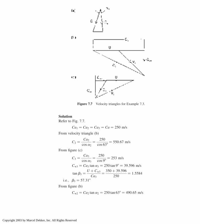
Solution
Refer to Fig. 7.7.
Ca1 ¼ Ca2 ¼ Ca3 ¼ Ca ¼ 250 m/s
From velocity triangle (b)
C2 ¼ Ca2
cosa2
¼ 250
cos 638¼ 550:67 m/s
From figure (c)
C3 ¼ Ca3
cosa3
¼ 250
cos 98¼ 253 m/s
Cw3 ¼ Ca3 tana3 ¼ 250 tan 98 ¼ 39:596 m/s
tanb3 ¼ U þ Cw3
Ca3¼ 350þ 39:596
250¼ 1:5584
i:e:; b3 ¼ 57:318
From figure (b)
Cw2 ¼ Ca2 tana2 ¼ 250 tan 638 ¼ 490:65 m/s
Figure 7.7 Velocity triangles for Example 7.3.
Chapter 7296
Copyright 2003 by Marcel Dekker, Inc. All Rights Reserved
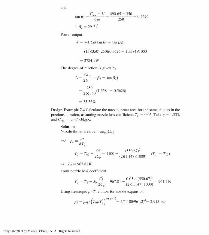
and
tanb2 ¼ Cw2 2 U
Ca2¼ 490:652 350
250¼ 0:5626
[ b2 ¼ 298210
Power output
W ¼ mUCað tanb2 þ tanb3Þ
¼ ð15Þð350Þð250Þð0:5626þ 1:5584Þ/1000
¼ 2784 kW
The degree of reaction is given by
L ¼ Ca
2Utanb3 2 tanb2
� �
¼ 250
2 £ 3501:55842 0:5626ð Þ
¼ 35:56%
Design Example 7.4 Calculate the nozzle throat area for the same data as in the
precious question, assuming nozzle loss coefficient, TN ¼ 0.05. Take g ¼ 1.333,
and Cpg ¼ 1.147 kJ/kgK.
Solution
Nozzle throat area, A ¼ m/r2Ca2
and r2 ¼ p2
RT2
T2 ¼ T02 2C22
2Cp
¼ 11002550:67ð Þ2
ð2Þð1:147Þð1000Þ T01 ¼ T02ð Þ
i.e., T2 ¼ 967:81K
From nozzle loss coefficient
T02 ¼ T2 2 lN
C22
2Cp
¼ 967:8120:05 £ 550:67ð Þ2ð2Þð1:147Þð1000Þ ¼ 961:2K
Using isentropic p–T relation for nozzle expansion
p2 ¼ p01= T01/T02
� �g/ g21ð Þ¼ 5/ 1100/961:2ð Þ4¼ 2:915 bar
Axial Flow and Radial Flow Gas Turbines 297
Copyright 2003 by Marcel Dekker, Inc. All Rights Reserved

Critical pressure ratio
p01/pc ¼ gþ 1
2
� �g/ g21ð Þ¼ 2:333
2
� �4
¼ 1:852
or p01/p2 ¼ 5/2:915 ¼ 1:715
Since p01p2
, p01pc, and therefore nozzle is unchoked.
Hence nozzle gas velocity at nozzle exit
C2 ¼ffiffiffiffiffiffiffiffiffiffiffiffiffiffiffiffiffiffiffiffiffiffiffiffiffiffiffiffiffiffiffiffiffiffiffi2Cpg T01 2 T2ð Þ q
¼ffiffiffiffiffiffiffiffiffiffiffiffiffiffiffiffiffiffiffiffiffiffiffiffiffiffiffiffiffiffiffiffiffiffiffiffiffiffiffiffiffiffiffiffiffiffiffiffiffiffiffiffiffiffiffiffiffiffiffiffiffiffiffiffiffiffiffiffið2Þð1:147Þð1000Þ 11002 967:81ð Þ½ �
p¼ 550:68 m/s
Therefore, nozzle throat area
A ¼ m
r2C2
; and r2 ¼ p2
RT2
¼ ð2:915Þð102Þð0:287Þð967:81Þ ¼ 1:05 kg/m3
Thus
A ¼ 15
ð1:05Þð550:68Þ ¼ 0:026 m2
Design Example 7.5 In a single-stage turbine, gas enters and leaves the turbine
axially. Inlet stagnation temperature is 1000K, and pressure ratio is 1.8 bar. Gas
leaving the stage with velocity 270m/s and blade speed at root is 290m/s. Stage
isentropic efficiency is 0.85 and degree of reaction is zero. Find the nozzle efflux
angle and blade inlet angle at the root radius.
Solution
Since L ¼ 0, therefore
L ¼ T2 2 T3
T1 2 T3;
hence
T2 ¼ T3
From isentropic p–T relation for expansion
T 003 ¼
T01
p01/p03� � g21ð Þ/g ¼
1000
1:8ð Þ0:249 ¼ 863:558 K
Chapter 7298
Copyright 2003 by Marcel Dekker, Inc. All Rights Reserved

Using turbine efficiency
T03 ¼ T01 2 ht T01 2 T 003
� �
¼ 10002 0:85ð10002 863:558Þ ¼ 884KIn order to find static temperature at turbine outlet, using static and
stagnation temperature relation
T3 ¼ T03 2C23
2Cpg
¼ 88422702
ð2Þð1:147Þð1000Þ ¼ 852K ¼ T2
Dynamic temperature
C22
2Cpg
¼ 10002 T2 ¼ 10002 852 ¼ 148K
C2 ¼ffiffiffiffiffiffiffiffiffiffiffiffiffiffiffiffiffiffiffiffiffiffiffiffiffiffiffiffiffiffiffiffiffiffiffiffiffiffiffiffiffiffiffiffiffiffiffið2Þð1:147Þð148Þð1000Þ½ �
p¼ 582:677 m/s
Since, CpgDTos ¼ U Cw3 þ Cw2ð Þ ¼ UCw2 ðCw3 ¼ 0Þ
Therefore, Cw2 ¼ ð1:147Þð1000Þ 10002 884ð Þ290
¼ 458:8 m/s
From velocity triangle
sina2 ¼ Cw2
C2
¼ 458:8
582:677¼ 0:787
That is, a2 ¼ 518540
tanb2 ¼ Cw2 2 U
Ca2¼ 458:82 290
C2 cosa2
¼ 458:82 290
582:677 cos 51:908¼ 0:47
i.e., b2 ¼ 25890
Design Example 7.6 In a single-stage axial flow gas turbine, gas enters the turbine
at a stagnation temperature and pressure of 1150K and 8 bar, respectively.
Isentropic efficiency of stage is equal to 0.88, mean blade speed is 300m/s, and
rotational speed is 240 rps. The gas leaves the stage with velocity 390m/s.
Assuming inlet and outlet velocities are same and axial, find the blade height at the
outlet conditions when the mass flow of gas is 34 kg/s, and temperature drop in the
stage is 145K.
Axial Flow and Radial Flow Gas Turbines 299
Copyright 2003 by Marcel Dekker, Inc. All Rights Reserved

Solution
Annulus area A is given by
A ¼ 2prmh
where h ¼ blade height
rm ¼ mean radius
As we have to find the blade height from the outlet conditions, in this case
annulus area is A3.
[ h ¼ A3
2prmUm ¼ pDmN
or Dm ¼ ðUmÞpN
¼ 300
ðpÞð240Þ ¼ 0:398
i.e., rm ¼ 0:199m
Temperature drop in the stage is given by
T01 2 T03 ¼ 145K
Hence T03 ¼ 11502 145 ¼ 1005K
T3 ¼ T03 2C23
2Cpg
¼ 100523902
ð2Þð1:147Þð1000Þ ¼ 938:697 K
Using turbine efficiency to find isentropic temperature drop
T 003 ¼ 11502
145
0:88¼ 985:23 K
Using isentropic p–T relation for expansion process
p03 ¼ p01
T01/T003
� �g/ g21ð Þ ¼8
1150/985:23ð Þ4 ¼8
1:856
i.e., p03 ¼ 4:31 bar
Also from isentropic relation
p3 ¼ p03
T 003/T3
� �g/ g21ð Þ ¼4:31
985:23/938:697ð Þ4 ¼4:31
1:214¼ 3:55 bar
r3 ¼ p3
RT3
¼ ð3:55Þð100Þð0:287Þð938:697Þ ¼ 1:32 kg/m3
A3 ¼ m
r3Ca3¼ 34
ð1:32Þð390Þ ¼ 0:066 m2
Chapter 7300
Copyright 2003 by Marcel Dekker, Inc. All Rights Reserved

Finally,
h ¼ A3
2prm¼ 0:066
ð2pÞð0:199Þ ¼ 0:053m
Design Example 7.7 The following data refer to a single-stage axial flow gas
turbine with convergent nozzle:
Inlet stagnation temperature; T01 1100K
Inlet stagnation pressure; p01 4 bar
Pressure ratio; p01/p03 1:9
Stagnation temperature drop 145K
Mean blade speed 345m/s
Mass flow; m 24 kg/s
Rotational speed 14; 500 rpm
Flow coefficient; F 0:75
Angle of gas leaving the stage 128
Cpg ¼ 1147 J/kgK; g ¼ 1:333; lN ¼ 0:05
Assuming the axial velocity remains constant and the gas velocity at inlet and
outlet are the same, determine the following quantities at the mean radius:
(1) The blade loading coefficient and degree of reaction
(2) The gas angles
(3) The nozzle throat area
Solution
ð1Þ C ¼ Cpg T01 2 T03ð ÞU 2
¼ ð1147Þð145Þ3452
¼ 1:4
Using velocity diagram
U/Ca ¼ tanb3 2 tana3
or tanb3 ¼ 1
Fþ tana3
¼ 1
0:75þ tan 128
b3 ¼ 57:18
From Equations (7.14) and (7.15), we have
C ¼ F tanb2 þ tanb3
� �
Axial Flow and Radial Flow Gas Turbines 301
Copyright 2003 by Marcel Dekker, Inc. All Rights Reserved
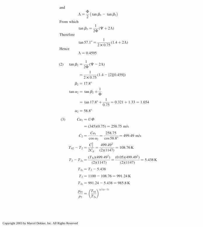
and
L ¼ F
2tanb3 2 tanb2
� �
From which
tanb3 ¼ 1
2FCþ 2Lð Þ
Therefore
tan 57:18 ¼ 1
2 £ 0:751:4þ 2Lð Þ
HenceL ¼ 0:4595
ð2Þ tanb2 ¼ 1
2FC2 2Lð Þ
¼ 1
2 £ 0:751:42 ½2�½0:459�ð Þ
b2 ¼ 17:88
tana2 ¼ tanb2 þ 1
F
¼ tan 17:88þ 1
0:75¼ 0:321þ 1:33 ¼ 1:654
a2 ¼ 58:88
ð3Þ Ca1 ¼ UF
¼ ð345Þð0:75Þ ¼ 258:75 m/s
C2 ¼ Ca1
cosa2
¼ 258:75
cos 58:88¼ 499:49 m/s
T02 2 T2 ¼ C22
2Cp
¼ 499:492
ð2Þð1147Þ ¼ 108:76K
T2 2 T2s ¼ ðTNÞð499:492Þð2Þð1147Þ ¼ ð0:05Þð499:492Þ
ð2Þð1147Þ ¼ 5:438K
T2s ¼ T2 2 5:438
T2 ¼ 11002 108:76 ¼ 991:24K
T2s ¼ 991:242 5:438 ¼ 985:8K
p01
p2¼ T01
T2s
� �g=ðg21Þ
Chapter 7302
Copyright 2003 by Marcel Dekker, Inc. All Rights Reserved

p2 ¼ 4 £ 985:8
1100
� �4
¼ 2:58
r2 ¼ p2
RT2
¼ ð2:58Þð100Þð0:287Þð991:24Þ ¼ 0:911 kg /m3
ð4Þ Nozzle throat area ¼ m
r1C1
¼ 24
ð0:907Þð499:49Þ ¼ 0:053m2
A1 ¼ m
r1Ca1¼ 24
ð0:907Þð258:75Þ ¼ 0:102m2
Design Example 7.8 A single-stage axial flow gas turbine with equal stage inlet
and outlet velocities has the following design data based on the mean diameter:
Mass flow 20 kg/s
Inlet temperature; T01 1150K
Inlet pressure 4 bar
Axial flow velocity constant through the stage 255m/s
Blade speed; U 345m/s
Nozzle efflux angle; a2 608
Gas-stage exit angle 128
Calculate (1) the rotor-blade gas angles, (2) the degree of reaction, blade-
loading coefficient, and power output and (3) the total nozzle throat area if the
throat is situated at the nozzle outlet and the nozzle loss coefficient is 0.05.
Solution
(1) From the velocity triangles
Cw2 ¼ Ca tana2
¼ 255 tan 608 ¼ 441:67 m/s
Cw3 ¼ Ca tana3 ¼ 255 tan 128 ¼ 55:2 m/s
Vw2 ¼ Cw2 2 U ¼ 441:672 345 ¼ 96:67 m/s
b2 ¼ tan21 Vw2
Ca¼ tan21 96:67
255¼ 20:88
Also Vw3 ¼ Cw3 þ U ¼ 345þ 55:2 ¼ 400:2 m/s
[ b3 ¼ tan21 Vw3
Ca¼ tan21 400:2
255¼ 57:58
Axial Flow and Radial Flow Gas Turbines 303
Copyright 2003 by Marcel Dekker, Inc. All Rights Reserved

ð2Þ L ¼ F
2tanb3 2 tanb2
� �
¼ 255
2 £ 345tan 57:58 2 tan 20:88ð Þ ¼ 0:44
C ¼ Ca
Utanb2 þ tanb3
� �
¼ 255
345tan 20:88þ tan 57:58ð Þ ¼ 1:44
Power W ¼ mU Cw2 þ Cw3ð Þ¼ ð20Þð345Þ 441:67þ 54:2ð Þ ¼ 3421:5 kW
ð3Þ lN ¼ Cp T2 2 T02
� �
12C22
;C2 ¼ Ca seca2 ¼ 255sec608 ¼ 510 m/s
or T2 2 T02 ¼
ð0:05Þð0:5Þð5102Þ1147
¼ 5:67
T2 ¼ T02 2C22
2Cp
¼ 115025102
ð2Þð1147Þ ¼ 1036:6K
T02 ¼ 1036:62 5:67 ¼ 1030:93K
p01
p2¼ T01
T2
� �g= g21ð Þ¼ 1150
1030:93
� �4
¼ 1:548
p2 ¼ 4
1:548¼ 2:584 bar
r2 ¼ p2
RT2
¼ 2:584 £ 100
0:287 £ 1036:6¼ 0:869 kg/m3
m ¼ r2A2C2
A2 ¼ 20
0:869 £ 510¼ 0:045m2
Chapter 7304
Copyright 2003 by Marcel Dekker, Inc. All Rights Reserved

Illustrative Example 7.9 A single-stage axial flow gas turbine has the
following data
Mean blade speed 340m/s
Nozzle exit angle 158
Axial velocity ðconstantÞ 105m/s
Turbine inlet temperature 9008C
Turbine outlet temperature 6708C
Degree of reaction 50%
Calculate the enthalpy drop per stage and number of stages required.
SolutionAt 50%,
a2 ¼ b3
a3 ¼ b2
C2 ¼ U
cos 158¼ 340
cos 158¼ 351:99 m/s
Heat drop in blade moving row ¼ C22 2 C2
3
2Cp
¼ ð351:99Þ2 2 ð105Þ2ð2Þð1147Þ
¼ 123896:962 11025
ð2Þð1147Þ¼ 49:2K
Therefore heat drop in a stage ¼ ð2Þð49:2Þ ¼ 98:41K
Number of stages ¼ 11732 943
98:41¼ 230
98:4¼ 2
Design Example 7.10 The following particulars relate to a single-stage turbine of
free vortex design:
Inlet temperature; T01 1100K
Inlet pressure; p01 4 bar
Mass flow 20 kg/s
Axial velocity at nozzle exit 250m/s
Blade speed at mean diameter 300m/s
Nozzle angle at mean diameter 258
Ratio of tip to root radius 1:4
Axial Flow and Radial Flow Gas Turbines 305
Copyright 2003 by Marcel Dekker, Inc. All Rights Reserved

The gas leaves the stage in an axial direction, find:
(1) The total throat area of the nozzle.
(2) The nozzle efflux angle at root and tip.
(3) The work done on the turbine blades.
Take
Cpg ¼ 1:147 kJ/kg K; g ¼ 1:33
SolutionFor no loss up to throat
p*
p01¼ 2
gþ 1
� �g=ðg21Þ¼ 2
2:33
� �4
¼ 0:543
p* ¼ 4 £ 0:543 ¼ 2:172 bar
Also T * ¼ 11002
2:33
� �4
¼ 944K
T01 ¼ T * þ C 2
2Cpg
C* ¼ffiffiffiffiffiffiffiffiffiffiffiffiffiffiffiffiffiffiffiffiffiffiffiffiffiffiffiffiffiffiffiffiffiffiffi
2Cpg T01 2 T *� �r
¼ffiffiffiffiffiffiffiffiffiffiffiffiffiffiffiffiffiffiffiffiffiffiffiffiffiffiffiffiffiffiffiffiffiffiffiffiffiffiffiffiffiffiffiffiffið2Þð1147Þ 11002 944ð Þ
p¼ 598 m/s
r* ¼ p*
RT *¼ ð2:172Þð100Þ
ð0:287Þð944Þ ¼ 0:802 kg/m3
(1) Throat area
A ¼ m
rC*¼ 20
ð0:802Þð598Þ ¼ 0:042m2
(2) Angle a1, at any radius r and a1m at the design radius rm are related by
the equation
tana1 ¼ rm
r1tana1m
Chapter 7306
Copyright 2003 by Marcel Dekker, Inc. All Rights Reserved

Given
Tip radius
Root radius¼ rt
rr¼ 1:4
[Mean radius
Root radius¼ 1:2
a1m ¼ 258
tana1r ¼ rmean
rroot£ tana1m
¼ 1:2 £ tan 258 ¼ 0:5596
[ a1r ¼ 29:238
tana1t ¼ rr
rt£ tana1r ¼ 1
1:4
� �ð0:5596Þ ¼ 0:3997
[ a1t ¼ 21:798
ð3Þ Cw2 ¼ rm
rrxCw2m ¼ rm
rr
Ca2
tana2m
¼ 1:2x250
tan 258¼ 643 m/s
W ¼ mUCw2 ¼ ð20Þð300Þð643Þ1000
¼ 3858 kW
7.8 RADIAL FLOW TURBINE
In Sec. 7.1 “Introduction to Axial Flow Turbines”, it was pointed out that in axial
flow turbines the fluid moves essentially in the axial direction through the rotor.
In the radial type the fluid motion is mostly radial. The mixed flow machine is
characterized by a combination of axial and radial motion of the fluid relative to
the rotor. The choice of turbine depends on the application, though it is not
always clear that any one type is superior. For small mass flows, the radial
machine can be made more efficient than the axial one. The radial turbine is
capable of a high-pressure ratio per stage than the axial one. However, multi-
staging is very much easier to arrange with the axial turbine, so that large overall
pressure ratios are not difficult to obtain with axial turbines. The radial flow
turbines are used in turbochargers for commercial (diesel) engines and fire
pumps. They are very compact, the maximum diameter being about 0.2m,
and run at very high speeds. In inward flow radial turbine, gas enters in the radial
direction and leaves axially at outlet. The rotor, which is usually manufactured of
Axial Flow and Radial Flow Gas Turbines 307
Copyright 2003 by Marcel Dekker, Inc. All Rights Reserved

Figure 7.9 Elements of a 908 inward flow radial gas turbine with inlet nozzle ring.
Figure 7.8 Radial turbine photograph of the rotor on the right.
Chapter 7308
Copyright 2003 by Marcel Dekker, Inc. All Rights Reserved

cast nickel alloy, has blades that are curved to change the flow from the radial to
the axial direction. Note that this turbine is like a single-faced centrifugal
compressor with reverse flow. Figures 7.8–7.10 show photographs of the radial
turbine and its essential parts.
7.9 VELOCITY DIAGRAMS ANDTHERMODYNAMIC ANALYSIS
Figure 7.11 shows the velocity triangles for this turbine. The same nomenclature
that we used for axial flow turbines, will be used here. Figure 7.12 shows the
Mollier diagram for a 908 flow radial turbine and diffuser.
As no work is done in the nozzle, we have h01 ¼ h02. The stagnation
pressure drops from p01 to p1 due to irreversibilities. The work done per unit mass
flow is given by Euler’s turbine equation
W t ¼ U2Cw2 2 U3Cw3ð Þ ð7:36ÞIf the whirl velocity is zero at exit then
W t ¼ U2Cw2 ð7:37Þ
Figure 7.10 A 908 inward flow radial gas turbine without nozzle ring.
Axial Flow and Radial Flow Gas Turbines 309
Copyright 2003 by Marcel Dekker, Inc. All Rights Reserved

Figure 7.12 Mollier chart for expansion in a 908 inward flow radial gas turbine.
Figure 7.11 Velocity triangles for the 908 inward flow radial gas turbine.
Chapter 7310
Copyright 2003 by Marcel Dekker, Inc. All Rights Reserved

For radial relative velocity at inlet
W t ¼ U22 ð7:38Þ
In terms of enthalpy drop
h02 2 h03 ¼ U2Cw2 2 U3Cw3
Using total-to-total efficiency
htt ¼ T01 2 T03
T01 2 T03 ss
;
efficiency being in the region of 80–90%
7.10 SPOUTING VELOCITY
It is that velocity, which has an associated kinetic energy equal to the isentropic
enthalpy drop from turbine inlet stagnation pressure p01 to the final exhaust
pressure. Spouting velocities may be defined depending upon whether total or
static conditions are used in the related efficiency definition and upon whether or
not a diffuser is included with the turbine. Thus, when no diffuser is used, using
subscript 0 for spouting velocity.
1
2C20 ¼ h01 2 h03 ss ð7:39Þ
or1
2C20 ¼ h01 2 h3 ss ð7:40Þ
for the total and static cases, respectively.
Now for isentropic flow throughout work done per unit mass flow
W ¼ U22 ¼ C2
0/2 ð7:41Þor U2/C0 ¼ 0:707 ð7:42ÞIn practice, U2/C0 lies in the range 0:68 ,
U2
C0
, 0:71.
7.11 TURBINE EFFICIENCY
Referring to Fig. 7.12, the total-to-static efficiency, without diffuser, is defined as
hts ¼ h01 2 h03
h01 2 h3 ss
¼ W
W þ 12C23 þ h3 2 h3ssð Þ þ h3s 2 h3 ssð Þ ð7:43Þ
Axial Flow and Radial Flow Gas Turbines 311
Copyright 2003 by Marcel Dekker, Inc. All Rights Reserved

Nozzle loss coefficient, jn, is defined as
jn ¼ Enthalpy loss in nozzle
Kinetic energy at nozzle exit
¼ h3s 2 h3 ss
0:5C22 T3/T2ð Þ ð7:44Þ
Rotor loss coefficient, jr, is defined as
jr ¼ h3 2 h3s
0:5V23
ð7:45Þ
But for constant pressure process,
T ds ¼ dh;
and, therefore
h3s 2 h3ss ¼ h2 h2sð Þ T3/T2ð ÞSubstituting in Eq. (7.43)
hts ¼ 1þ 1
2C2
3 þ V23jr þ C2jnT3/T2
� �W
� �21
ð7:46Þ
Using velocity triangles
C2 ¼ U2 coseca2;V3 ¼ U3 cosecb3;C3 ¼ U3 cotb3;W ¼ U22
Substituting all those values in Eq. (7.44) and noting that U3 ¼ U2 r3/r2, then
hts ¼ 1þ 1
2jn
T3
T2
cosec2a2 þ r3
r2
� �2
jr cosec2b3 þ cot2b3
� �( )" #21
ð7:47ÞTaking mean radius, that is,
r3 ¼ 1
2r3t þ r3hð Þ
Using thermodynamic relation for T3/T2, we get
T3
T2
¼ 121
2g2 1� � U2
a2
� �2
12 cot2a2 þ r3
r2
� �2
cot2b3
" #
But the above value of T3/T2 is very small, and therefore usually neglected. Thus
hts ¼ 1þ 1
2jncosec
2a2 þ r3 av
r2
� �2
jr cosec2b3 av þ cot2b3 av
� �( )" #21
ð7:48Þ
Chapter 7312
Copyright 2003 by Marcel Dekker, Inc. All Rights Reserved

Equation (7.46) is normally used to determine total-to-static efficiency. The hts
can also be found by rewriting Eq. (7.43) as
hts ¼ h01 2 h03
h01 2 h3 ss¼ h01 2 h3 ssð Þ2 h03 2 h3ð Þ2 h3 2 h3sð Þ2 h3s 2 h3 ssð Þ
h01 2 h3ssð Þ¼ 12 C2
3 þ jnC22 þ jrV
23
� �/C2
0ð7:49Þ
where spouting velocity C0 is given by
h01 2 h3 ss ¼ 1
2C20 ¼ CpT01 12 p3/p01
� �g21=gh i
ð7:50ÞThe relationship between hts and htt can be obtained as follows:
W ¼ U22 ¼ htsW ts ¼ hts h01 2 h3ssð Þ; then
htt ¼ W
W ts 212C23
¼ 1
1hts2
C23
2W
[1
htt
¼ 1
hts
2C23
2W¼ 1
hts
21
2
r3av
r22 cotb3av
� �2
ð7:51Þ
Loss coefficients usually lie in the following range for 908 inward flow turbines
jn ¼ 0:063–0:235
and
jr ¼ 0:384–0:777
7.12 APPLICATION OF SPECIFIC SPEED
We have already discussed the concept of specific speed Ns in Chapter 1 and
some applications of it have been made already. The concept of specific speed
was applied almost exclusively to incompressible flow machines as an important
parameter in the selection of the optimum type and size of unit. The volume flow
rate through hydraulic machines remains constant. But in radial flow gas turbine,
volume flow rate changes significantly, and this change must be taken into
account. According to Balje, one suggested value of volume flow rate is that at
the outlet Q3.
Using nondimensional form of specific speed
Ns ¼ NQ1/23
ðDh00Þ3/4
ð7:52Þ
where N is in rev/s, Q3 is in m3/s and isentropic total-to-total enthalpy drop
(from turbine inlet to outlet) is in J/kg. For the 908 inward flow radial turbine,
Axial Flow and Radial Flow Gas Turbines 313
Copyright 2003 by Marcel Dekker, Inc. All Rights Reserved

U2 ¼ pND2 and Dh0s ¼ 12C20; factorizing the Eq. (7.52)
Ns ¼ Q1/23
12C20
� �3/4U2
pD2
� �U2
pND2
� �1/2
¼ffiffiffi2
pp
� �3/2U2
C0
� �3/2Q3
ND32
� �1/2
ð7:53Þ
For 908 inward flow radial turbine, U2/C0 ¼ 1ffiffi2
p ¼ 0:707; substituting this value
in Eq. (7.53),
Ns ¼ 0:18Q3
ND32
� �1/2
; rev ð7:54Þ
Equation (7.54) shows that specific speed is directly proportional to the square
root of the volumetric flow coefficient. Assuming a uniform axial velocity at rotor
exit C3, so that Q3 ¼ A3C3, rotor disc area Ad ¼ pD22/4, then
N ¼ U2/ pD2ð Þ ¼ C0
ffiffiffi2
p2pD2
Q3
ND32
¼ A3C32pD2ffiffiffi2
pC0D
22
¼ A3
Ad
C3
C0
p2
2ffiffiffi2
p
Therefore,
Ns ¼ 0:336C3
C0
� �12 A3
Ad
� �12
; rev ð7:55Þ
¼ 2:11C3
C0
� �12 A3
Ad
� �12
; rad ð7:56Þ
Suggested values for C3/Co and A3/Ad are as follows:
0:04 , C3/C0 , 0:3
0:1 , A3/Ad , 0:5
Then 0:3 , Ns , 1:1; rad
Thus theNs range is very small and Fig. 7.13 shows the variation of efficiencywith
Ns, where it is seen to match the axial flow gas turbine over the limited range ofNs.
Design Example 7.11 A small inward radial flow gas turbine operates at its
design point with a total-to-total efficiency of 0.90. The stagnation pressure and
temperature of the gas at nozzle inlet are 310 kPa and 1145K respectively. The
flow leaving the turbine is diffused to a pressure of 100 kPa and the velocity of
Chapter 7314
Copyright 2003 by Marcel Dekker, Inc. All Rights Reserved

flow is negligible at that point. Given that the Mach number at exit from the
nozzles is 0.9, find the impeller tip speed and the flow angle at the nozzle exit.
Assume that the gas enters the impeller radially and there is no whirl at the
impeller exit. Take
Cp ¼ 1:147 kJ/kgK; g ¼ 1:333:
Solution
The overall efficiency of turbine from nozzle inlet to diffuser outlet is
given by
htt ¼ T01 2 T03
T01 2 T03 ss
Turbine work per unit mass flow
W ¼ U22 ¼ Cp T01 2 T03ð Þ; Cw3 ¼ 0ð Þ
Now using isentropic p–T relation
T01 12T03ss
T01
� �¼ T01 12
p03
p01
� �g21=g" #
Therefore
U22 ¼ httCpT01 12
p03
p01
� �g21=g" #
¼ 0:9 £ 1147 £ 1145 12100
310
� �0:2498" #
[ Impeller tip speed, U2 ¼ 539.45m/s
Figure 7.13 Variation of efficiency with dimensionless specific speed.
Axial Flow and Radial Flow Gas Turbines 315
Copyright 2003 by Marcel Dekker, Inc. All Rights Reserved

The Mach number of the absolute flow velocity at nozzle exit is given by
M ¼ C1
a1¼ U1
a1 sina1
Since the flow is adiabatic across the nozzle, we have
T01 ¼ T02 ¼ T2 þ C22
2Cp
¼ T2 þ U22
2Cp sin2a2
or T2
T01
¼ 12U2
2
2CpT01 sin2a2
; but Cp ¼ gR
g2 1
[T2
T01
¼ 12U2
2 g2 1� �
2gRT01 sin2a2
¼ 12U2
2 g2 1� �
2a201 sin2a2
But T2
T01
� �2
¼ a2
a01¼ a2
a02since T01 ¼ T02
and a2
a02¼ U2
M2a02 sina2
[U2
M2a02 sina2
� �2
¼ 12U2
2 g2 1� �
2a202 sin2a2
and 1 ¼ U2
a02 sina2
� �2 g2 1� �
2þ 1
M22
� �
or sin 2a2 ¼ U2
a02
� �2 g2 1� �
2þ 1
M22
� �
But a202 ¼ gRT02 ¼ ð1:333Þð287Þð1145Þ ¼ 438043m2/ s 2
[ sin 2a2 ¼ 539:452
438043
0:333
2þ 1
0:92
� �¼ 0:9311
Therefore nozzle angle a2 ¼ 758
Illustrative Example 7.12 The following particulars relate to a small inward
flow radial gas turbine.
Rotor inlet tip diameter 92mm
Rotor outlet tip diameter 64mm
Rotor outlet hub diameter 26mm
Ratio C3/C0 0:447
Chapter 7316
Copyright 2003 by Marcel Dekker, Inc. All Rights Reserved

Ratio U2/C0 ðidealÞ 0:707
Blade rotational speed 30; 500 rpm
Density at impeller exit 1:75 kg/m3
Determine
(1) The dimensionless specific speed of the turbine.
(2) The volume flow rate at impeller outlet.
(3) The power developed by the turbine.
Solution(1) Dimensionless specific speed is
Ns ¼ 0:336C3
C0
� �12 A3
Ad
� �12
; rev
Now
A3 ¼ p D23t 2 D2
3h
� �
4
¼ p 0:0642 2 0:0262� �
4¼ ð2:73Þð1023Þ m2
Ad ¼ pD22
4¼ p
4
� �ð0:0922Þ ¼ ð6:65Þð1023Þ m2
Dimensionless specific speed
Ns ¼ 0:336½0:447�½2:73�
6:65
� �12
¼ 0:144 rev
¼ 0:904 rad
(2) The flow rate at outlet for the ideal turbine is given by Eq. (7.54).
Ns ¼ 0:18Q3
ND32
� �1=2
0:144 ¼ 0:18½Q3�½60�
½30; 500�½0:0923�� �1=2
Hence
Q3 ¼ 0:253m3 /s
Axial Flow and Radial Flow Gas Turbines 317
Copyright 2003 by Marcel Dekker, Inc. All Rights Reserved

(3) The power developed by the turbine is given by
W t ¼ _mU23
¼ r3Q3U23
¼ 1:75 £ 0:253 £ pND2
60
� �2
¼ 1:75 £ 0:253 £ ½p�½30; 500�½0:092�60
� �2
¼ 9:565 kW
PROBLEMS
7.1 A single-stage axial flow gas turbine has the following data:
Inlet stagnation temperature 1100K
The ratio of static pressure at the
nozzle exit to the stagnation
pressure at the nozzle inlet 0:53
Nozzle efficiency 0:93
Nozzle angle 208
Mean blade velocity 454m/s
Rotor efficiency 0:90
Degree of reaction 50%
Cpg ¼ 1:147 kJ/kgK; g ¼ 1:33
Find (1) the work output per kg/s of air flow, (2) the ratio of the static
pressure at the rotor exit to the stagnation pressure at the nozzle inlet,
and (3) the total-to-total stage efficiency.
(282 kW, 0.214, 83.78%)
7.2 Derive an equation for the degree of reaction for a single-stage axial flow
turbine and show that for 50% reaction blading a2 ¼ b3 and a3 ¼ b2.
7.3 For a free-vortex turbine blade with an impulse hub show that degree of
reaction
L ¼ 12rh
r
� �2
where rh is the hub radius and r is any radius.
Chapter 7318
Copyright 2003 by Marcel Dekker, Inc. All Rights Reserved

7.4 A 50% reaction axial flow gas turbine has a total enthalpy drop of 288 kJ/kg.
The nozzle exit angle is 708. The inlet angle to the rotating blade row is
inclined at 208with the axial direction. The axial velocity is constant throughthe stage. Calculate the enthalpy drop per row of moving blades and the
number of stages required when mean blade speed is 310m/s. Take Cpg ¼1:147 kJ/kgK; g ¼ 1:33:
(5 stages)
7.5 Show that for zero degree of reaction, blade-loading coefficient, C ¼ 2.
7.6 The inlet stagnation temperature and pressure for an axial flow gas turbine
are 1000K and 8 bar, respectively. The exhaust gas pressure is 1.2 bar and
isentropic efficiency of turbine is 85%. Assume gas is air, find the exhaust
stagnation temperature and entropy change of the gas.
(644K, 20.044 kJ/kgK)
7.7 The performance date from inward radial flow exhaust gas turbine are as
follows:
Stagnation pressure at inlet to nozzles; p01 705 kPa
Stagnation temperature at inlet to nozzles; T01 1080K
Static pressure at exit from nozzles; p2 515 kPa
Static temperature at exit from nozzles; T2 1000K
Static pressure at exit from rotor; p3 360 kPa
Static temperature at exit from rotor; T3 923K
Stagnation temperature at exit from rotor; T03 925K
Ratio r2 avr2
0:5
Rotational speed; N 25; 500 rpm
The flow into the rotor is radial and at exit the flow is axial at all radii.
Calculate (1) the total-to-static efficiency of the turbine, (2) the impeller tip
diameter, (3) the enthalpy loss coefficient for the nozzle and rotor rows, (4)
the blade outlet angle at the mean diameter, and (5) the total-to-total
efficiency of the turbine.
[(1) 93%, (2) 0.32m, (3) 0.019, 0.399, (4) 72.28, (5) 94%]
NOTATION
A area
C absolute velocity
Axial Flow and Radial Flow Gas Turbines 319
Copyright 2003 by Marcel Dekker, Inc. All Rights Reserved

C0 spouting velocity
h enthalpy, blade height
N rotation speed
Ns specific speed
P pressure
rm mean radius
T temperature
U rotor speed
V relative velocity
YN nozzle loss coefficient in terms of pressure
a angle with absolute velocity
b angle with relative velocity
DT0s stagnation temperature drop in the stage
DTs static temperature drop in the stage
1n nozzle loss coefficient in radial flow turbine
1r rotor loss coefficient in radial flow turbine
f flow coefficient
hs isentropic efficiency of stage
L degree of reaction
Chapter 7320
Copyright 2003 by Marcel Dekker, Inc. All Rights Reserved


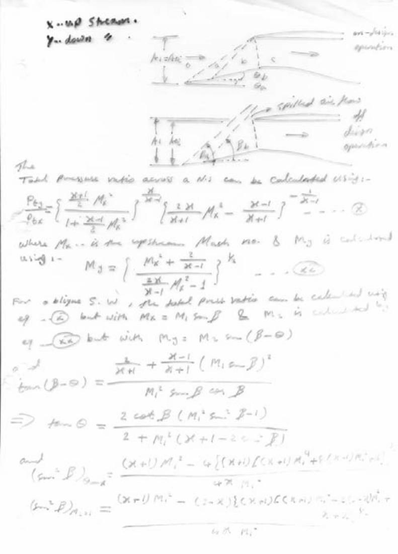


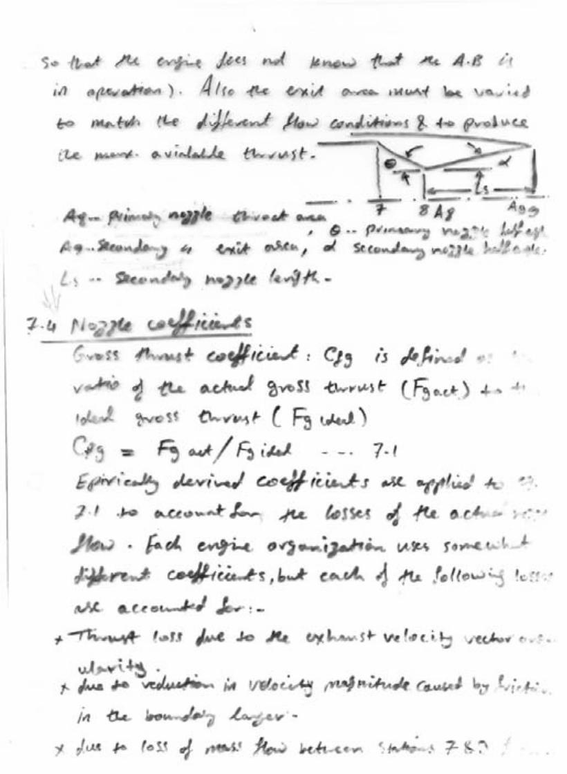
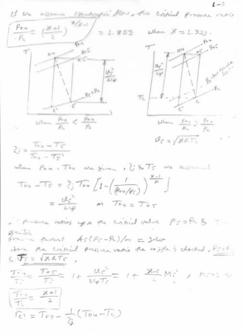

Related Documents


