Lecture slides by Kevin Wayne Copyright © 2005 Pearson-Addison Wesley http://www.cs.princeton.edu/~wayne/kleinberg-tardos Last updated on Feb 18, 2013 6:08 AM 4. G REEDY A LGORITHMS II ‣ Dijkstra's algorithm ‣ minimum spanning trees ‣ Prim, Kruskal, Boruvka ‣ single-link clustering ‣ min-cost arborescences

Welcome message from author
This document is posted to help you gain knowledge. Please leave a comment to let me know what you think about it! Share it to your friends and learn new things together.
Transcript
Lecture slides by Kevin WayneCopyright © 2005 Pearson-Addison Wesley
http://www.cs.princeton.edu/~wayne/kleinberg-tardos
Last updated on Feb 18, 2013 6:08 AM
4. GREEDY ALGORITHMS II
‣ Dijkstra's algorithm
‣ minimum spanning trees
‣ Prim, Kruskal, Boruvka
‣ single-link clustering
‣ min-cost arborescences

SECTION 4.4
4. GREEDY ALGORITHMS II
‣ Dijkstra's algorithm
‣ minimum spanning trees
‣ Prim, Kruskal, Boruvka
‣ single-link clustering
‣ min-cost arborescences
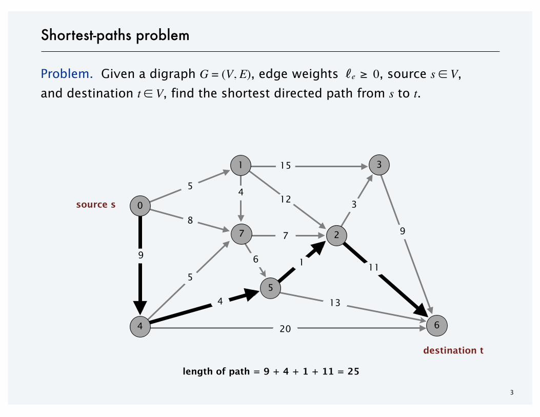
Problem. Given a digraph G = (V, E), edge weights ℓe ≥ 0, source s ∈ V,
and destination t ∈ V, find the shortest directed path from s to t.
Shortest-paths problem
3
7
1 3
source s
6
8
5
7
54
15
312
20
13
9
length of path = 9 + 4 + 1 + 11 = 25
destination t
0
4
5
2
6
9
4
1 11

Car navigation
4
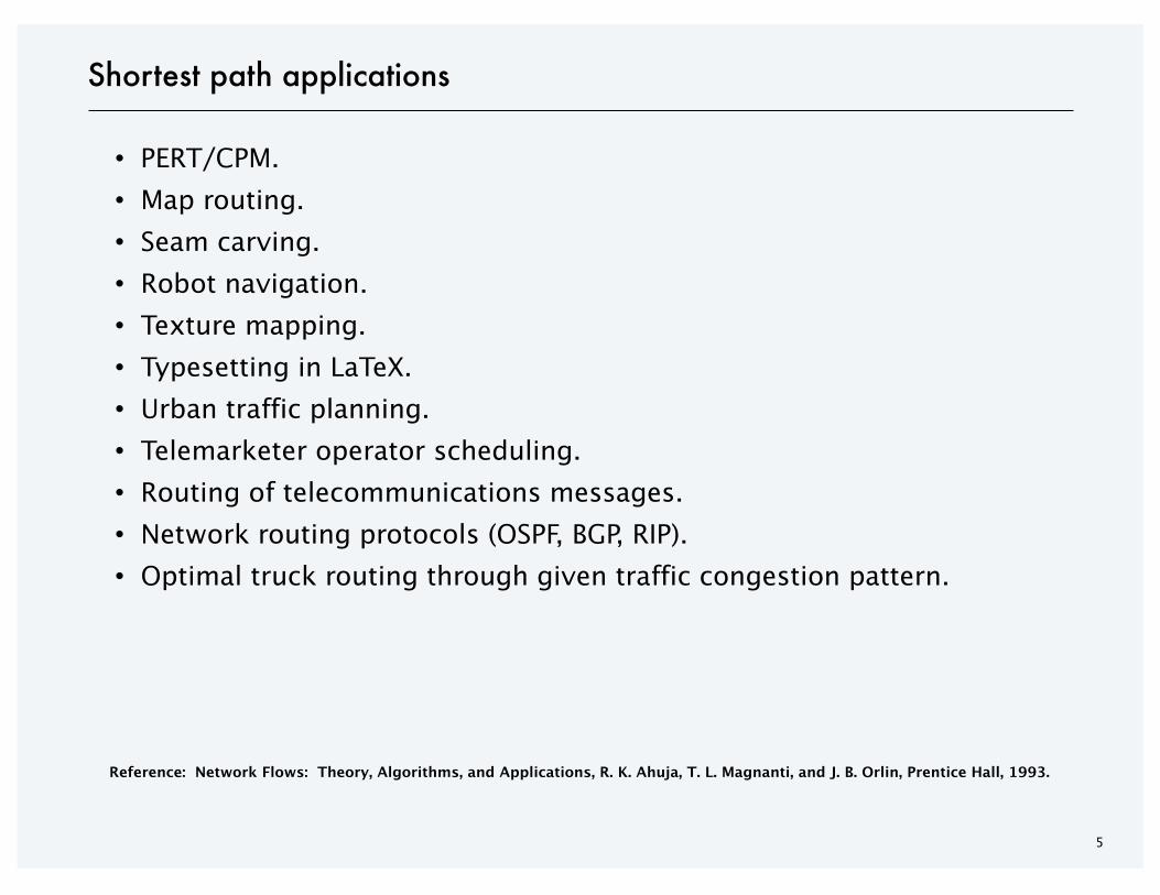
・PERT/CPM.
・Map routing.
・Seam carving.
・Robot navigation.
・Texture mapping.
・Typesetting in LaTeX.
・Urban traffic planning.
・Telemarketer operator scheduling.
・Routing of telecommunications messages.
・Network routing protocols (OSPF, BGP, RIP).
・Optimal truck routing through given traffic congestion pattern.
5
Reference: Network Flows: Theory, Algorithms, and Applications, R. K. Ahuja, T. L. Magnanti, and J. B. Orlin, Prentice Hall, 1993.
Shortest path applications

Greedy approach. Maintain a set of explored nodes S for which
algorithm has determined the shortest path distance d(u) from s to u.
・Initialize S = { s }, d(s) = 0.
・Repeatedly choose unexplored node v which minimizes
6
Dijkstra's algorithm
s
v
uS
shortest path to some node u in explored part, followed by a single edge (u, v)
d(u)ℓe

Greedy approach. Maintain a set of explored nodes S for which
algorithm has determined the shortest path distance d(u) from s to u.
・Initialize S = { s }, d(s) = 0.
・Repeatedly choose unexplored node v which minimizes
add v to S, and set d(v) = π(v).
7
Dijkstra's algorithm
s
v
uS
d(u)ℓe
d(v)
shortest path to some node u in explored part, followed by a single edge (u, v)

Invariant. For each node u ∈ S, d(u) is the length of the shortest s↝u path.
Pf. [ by induction on | S | ]Base case: | S | = 1 is easy since S = { s } and d(s) = 0.
Inductive hypothesis: Assume true for | S | = k ≥ 1.
・Let v be next node added to S, and let (u, v) be the final edge.
・The shortest s↝u path plus (u, v) is an s↝v path of length π(v).
・Consider any s↝v path P. We show that it is no shorter than π(v).
・Let (x, y) be the first edge in P that leaves S,
and let P' be the subpath to x.
・P is already too long as soon as it reaches y.
S
s
8
Dijkstra's algorithm: proof of correctness
ℓ(P) ≥ ℓ(P') + ℓ(x, y)
nonnegativeweights
v
u
y
P
P'x
Dijkstra chose vinstead of y
≥ π (v)
definitionof π(y)
≥ π (y)
inductivehypothesis
≥ d(x) + ℓ(x, y) ▪
9
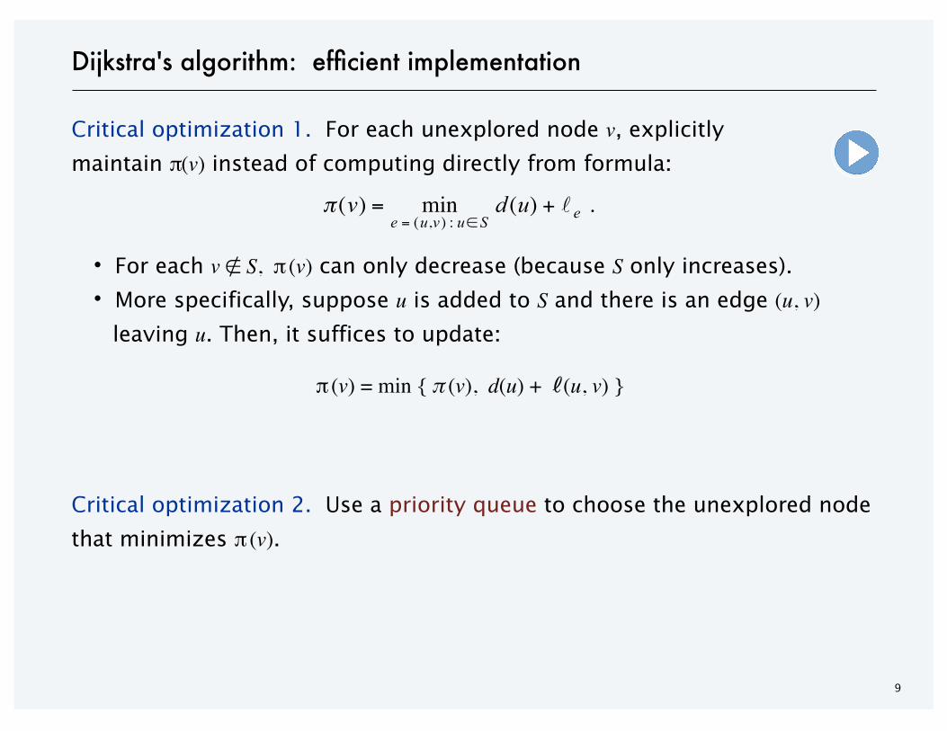
Dijkstra's algorithm: efficient implementation
Critical optimization 1. For each unexplored node v, explicitly
maintain π(v) instead of computing directly from formula:
・For each v ∉ S, π (v) can only decrease (because S only increases).
・More specifically, suppose u is added to S and there is an edge (u, v) leaving u. Then, it suffices to update:
Critical optimization 2. Use a priority queue to choose the unexplored node
that minimizes π (v).
€
π (v) = mine = (u,v) : u∈ S
d (u) + e .
π (v) = min { π (v), d(u) + ℓ(u, v) }
10
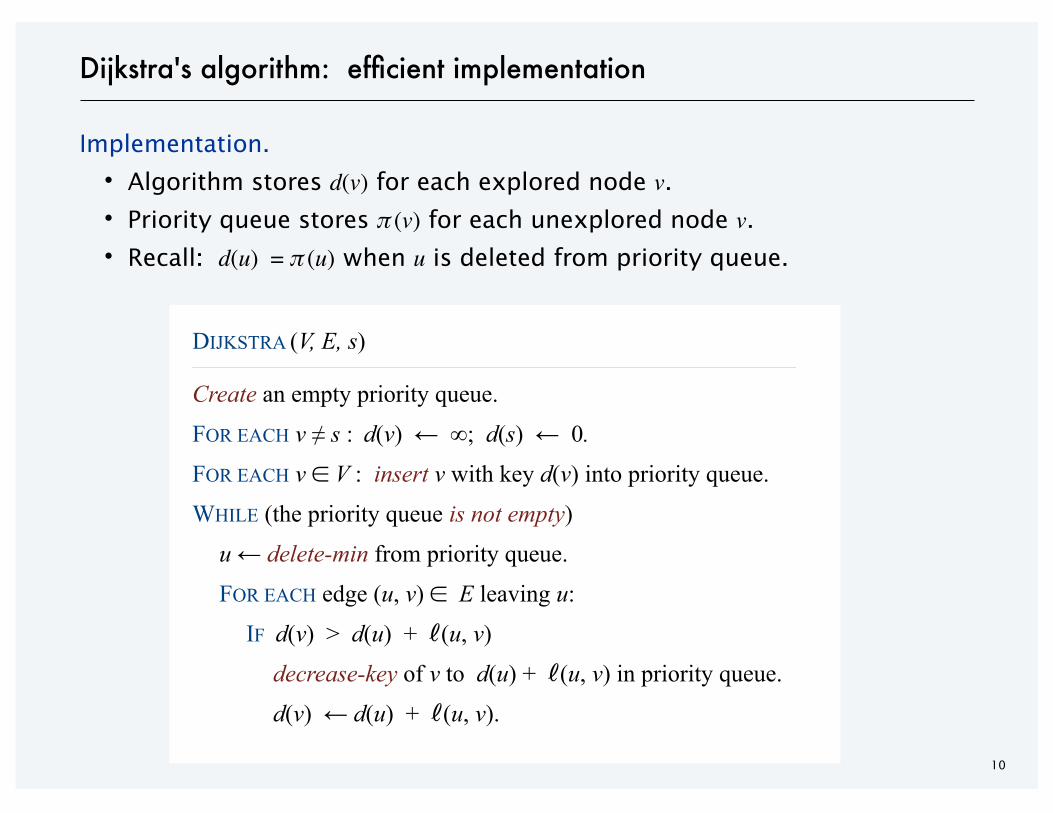
Dijkstra's algorithm: efficient implementation
Implementation.
・Algorithm stores d(v) for each explored node v.
・Priority queue stores π (v) for each unexplored node v.
・Recall: d(u) = π (u) when u is deleted from priority queue.
DIJKSTRA (V, E, s) _________________________________________________________________________________________________________________________________________________________________________________________________________________________________________________________________________________________________________________________________________________________________________________________________________________________________________________________________________________________________________________________________________________________________________________________________________________________________________________________________________________________________________________________________________________________________________________________________________________________________________________________________________________________________________________________________________________________________________________________________________________________________________________________________________________________________________________________________________________________________________________________________________________________________________________________
Create an empty priority queue.
FOR EACH v ≠ s : d(v) ← ∞; d(s) ← 0.
FOR EACH v ∈ V : insert v with key d(v) into priority queue.
WHILE (the priority queue is not empty)
u ← delete-min from priority queue.
FOR EACH edge (u, v) ∈ E leaving u:
IF d(v) > d(u) + ℓ(u, v)
decrease-key of v to d(u) + ℓ(u, v) in priority queue.
d(v) ← d(u) + ℓ(u, v)._________________________________________________________________________________________________________________________________________________________________________________________________________________________________________________________________________________________________________________________________________________________________________________________________________________________________________________________________________________________________________________________________________________________________________________________________________________________________________________________________________________________________________________________________________________________________________________________________________________________________________________________________________________________________________________________________________________________________________________________________________________________________________________________________________________________________________________________________________________________________________________________________________________________________________________________
11
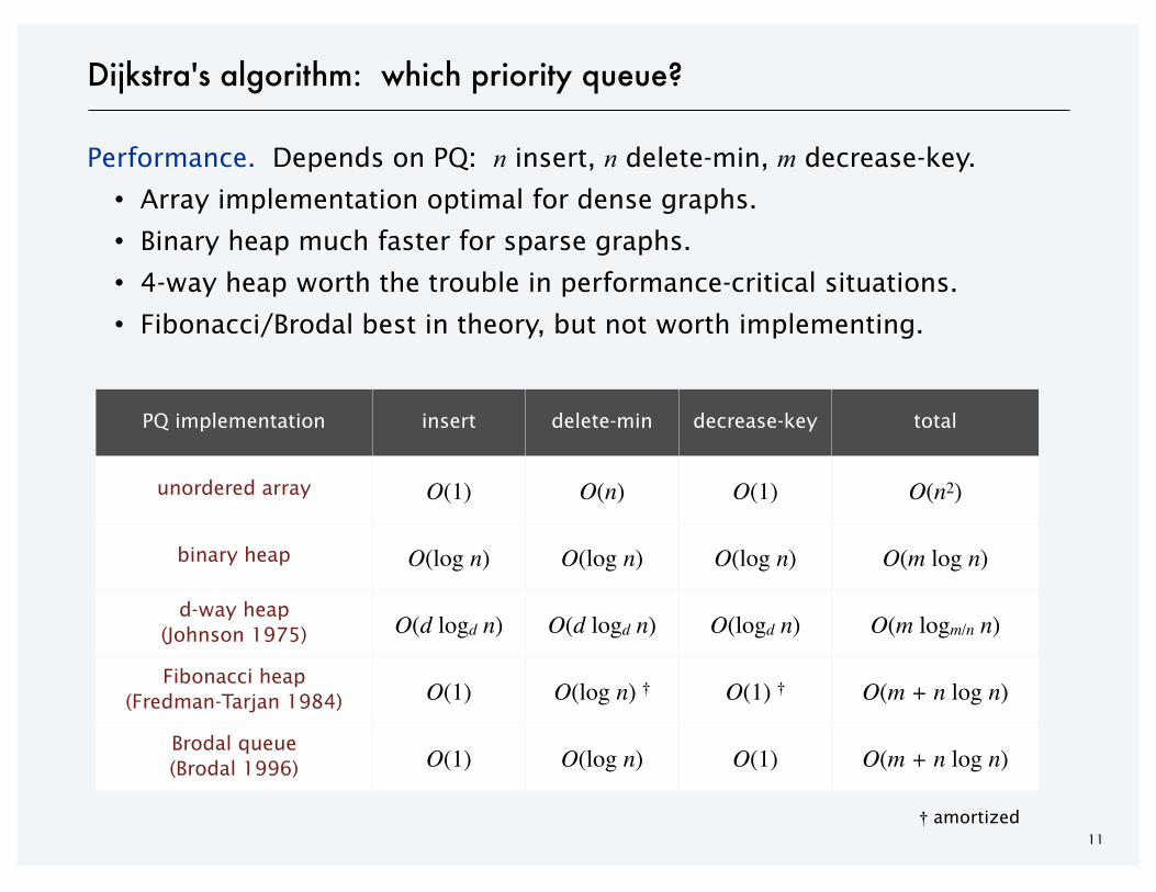
Performance. Depends on PQ: n insert, n delete-min, m decrease-key.
・Array implementation optimal for dense graphs.
・Binary heap much faster for sparse graphs.
・4-way heap worth the trouble in performance-critical situations.
・Fibonacci/Brodal best in theory, but not worth implementing.
Dijkstra's algorithm: which priority queue?
PQ implementation insert delete-min decrease-key total
unordered array O(1) O(n) O(1) O(n2)
binary heap O(log n) O(log n) O(log n) O(m log n)
d-way heap(Johnson 1975) O(d logd n) O(d logd n) O(logd n) O(m logm/n n)
Fibonacci heap(Fredman-Tarjan 1984) O(1) O(log n) † O(1) † O(m + n log n)
Brodal queue(Brodal 1996) O(1) O(log n) O(1) O(m + n log n)
† amortized

Dijkstra's algorithm and proof extend to several related problems:
・Shortest paths in undirected graphs: d(v) ≤ d(u) + ℓ(u, v).
・Maximum capacity paths: d(v) ≥ min { π (u), c(u, v) }.
・Maximum reliability paths: d(v) ≥ d(u) 𐄂 γ(u, v) .
・…
Key algebraic structure. Closed semiring (tropical, bottleneck, Viterbi).
12
Extensions of Dijkstra's algorithm
s
v
uS
d(u)ℓe
4. GREEDY ALGORITHMS II
‣ Dijkstra's algorithm
‣ minimum spanning trees
‣ Prim, Kruskal, Boruvka
‣ single-link clustering
‣ min-cost arborescences
SECTION 6.1
14
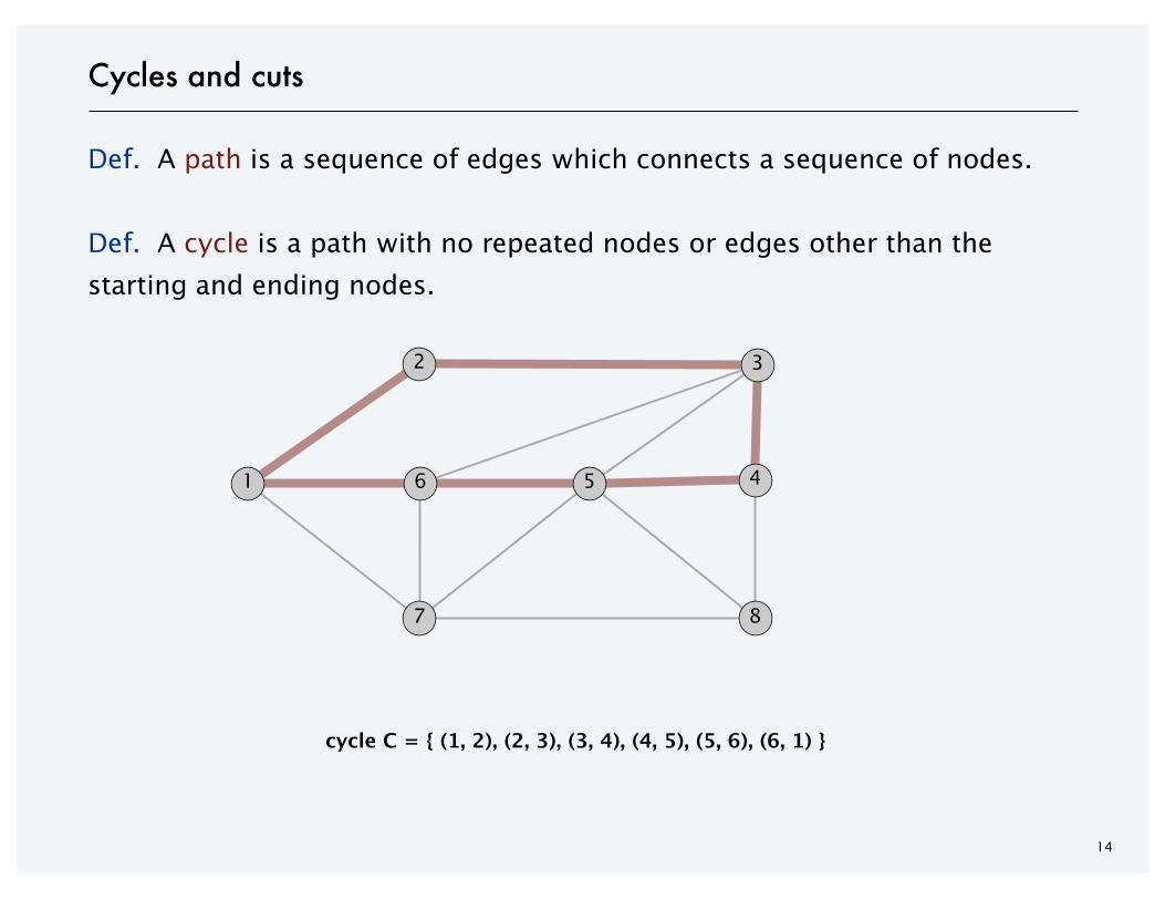
Cycles and cuts
Def. A path is a sequence of edges which connects a sequence of nodes.
Def. A cycle is a path with no repeated nodes or edges other than the
starting and ending nodes.
1
2 3
4
8
56
7
cycle C = { (1, 2), (2, 3), (3, 4), (4, 5), (5, 6), (6, 1) }
15
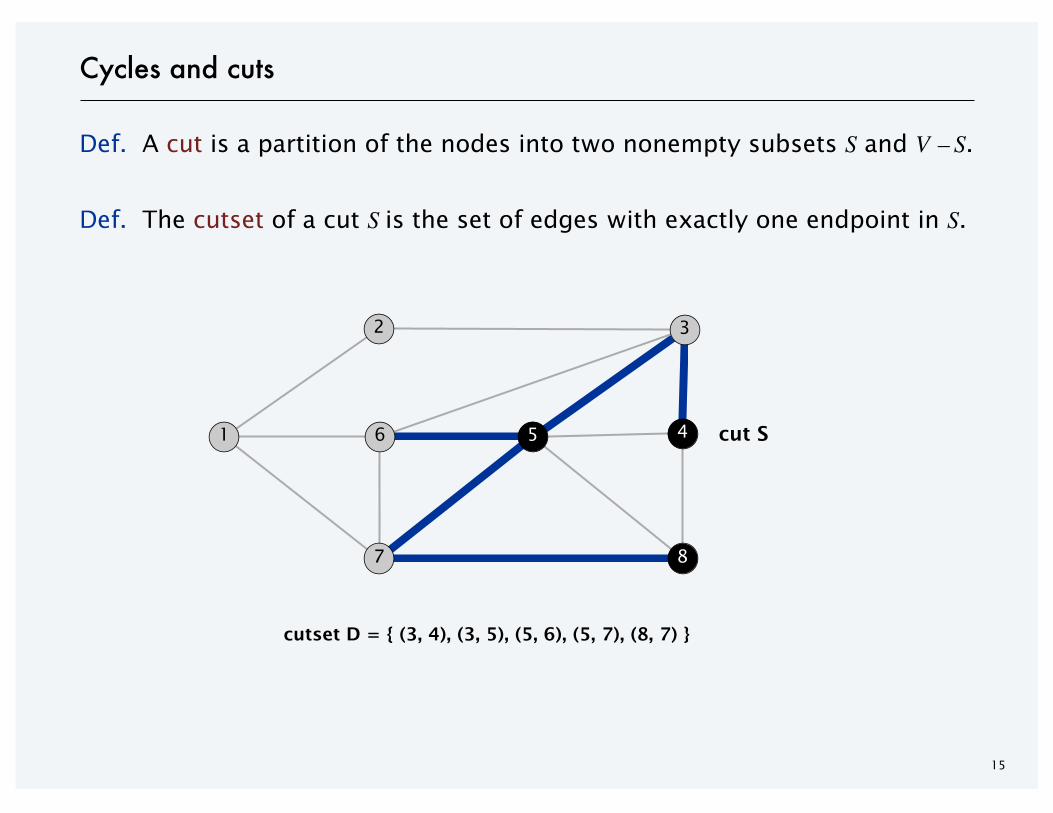
Cycles and cuts
Def. A cut is a partition of the nodes into two nonempty subsets S and V – S.
Def. The cutset of a cut S is the set of edges with exactly one endpoint in S.
1
2 3
4
8
56
7
cutset D = { (3, 4), (3, 5), (5, 6), (5, 7), (8, 7) }
cut S
16
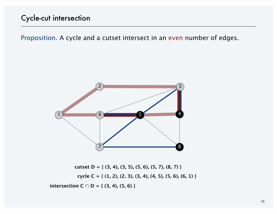
Cycle-cut intersection
Proposition. A cycle and a cutset intersect in an even number of edges.
1
2 3
4
8
56
7
cutset D = { (3, 4), (3, 5), (5, 6), (5, 7), (8, 7) }
intersection C ∩ D = { (3, 4), (5, 6) }
cycle C = { (1, 2), (2, 3), (3, 4), (4, 5), (5, 6), (6, 1) }
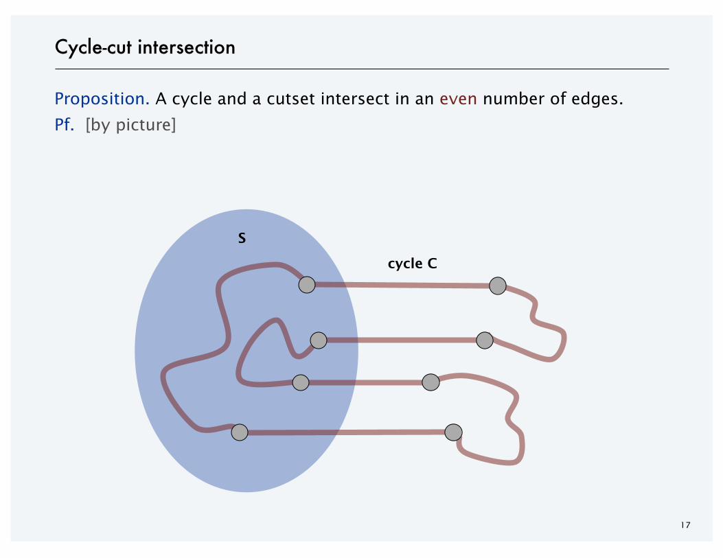
Proposition. A cycle and a cutset intersect in an even number of edges.
Pf. [by picture]
17
Cycle-cut intersection
cycle C
S
18
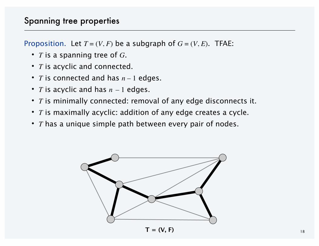
Spanning tree properties
Proposition. Let T = (V, F) be a subgraph of G = (V, E). TFAE:
・T is a spanning tree of G.
・T is acyclic and connected.
・T is connected and has n – 1 edges.
・T is acyclic and has n – 1 edges.
・T is minimally connected: removal of any edge disconnects it.
・T is maximally acyclic: addition of any edge creates a cycle.
・T has a unique simple path between every pair of nodes.
T = (V, F)
19
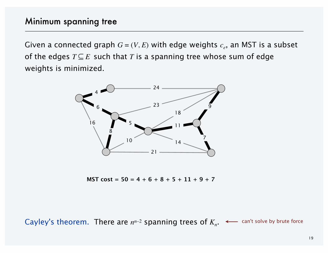
Minimum spanning tree
Given a connected graph G = (V, E) with edge weights ce, an MST is a subset
of the edges T ⊆ E such that T is a spanning tree whose sum of edge
weights is minimized.
Cayley's theorem. There are nn–2 spanning trees of Kn. can't solve by brute force
MST cost = 50 = 4 + 6 + 8 + 5 + 11 + 9 + 7
16
4
6 23
10
21
14
24
189
7
115
8
20
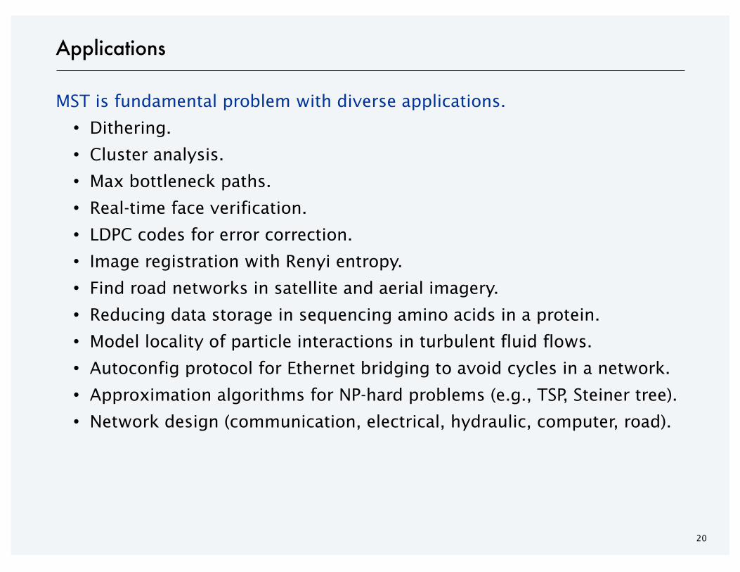
Applications
MST is fundamental problem with diverse applications.
・Dithering.
・Cluster analysis.
・Max bottleneck paths.
・Real-time face verification.
・LDPC codes for error correction.
・Image registration with Renyi entropy.
・Find road networks in satellite and aerial imagery.
・Reducing data storage in sequencing amino acids in a protein.
・Model locality of particle interactions in turbulent fluid flows.
・Autoconfig protocol for Ethernet bridging to avoid cycles in a network.
・Approximation algorithms for NP-hard problems (e.g., TSP, Steiner tree).
・Network design (communication, electrical, hydraulic, computer, road).
21
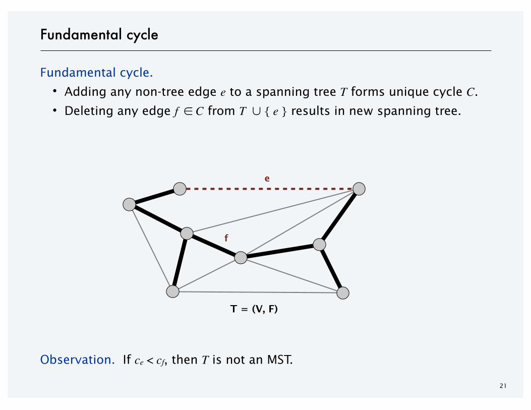
Fundamental cycle
Fundamental cycle.
・Adding any non-tree edge e to a spanning tree T forms unique cycle C.
・Deleting any edge f ∈ C from T ∪ { e } results in new spanning tree.
Observation. If ce < cf, then T is not an MST.
T = (V, F)
e
f

22
Fundamental cutset
Fundamental cutset.
・Deleting any tree edge f from a spanning tree T divide nodes into
two connected components. Let D be cutset.
・Adding any edge e ∈ D to T – { f } results in new spanning tree.
Observation. If ce < cf, then T is not an MST.
T = (V, F)
e
f
23
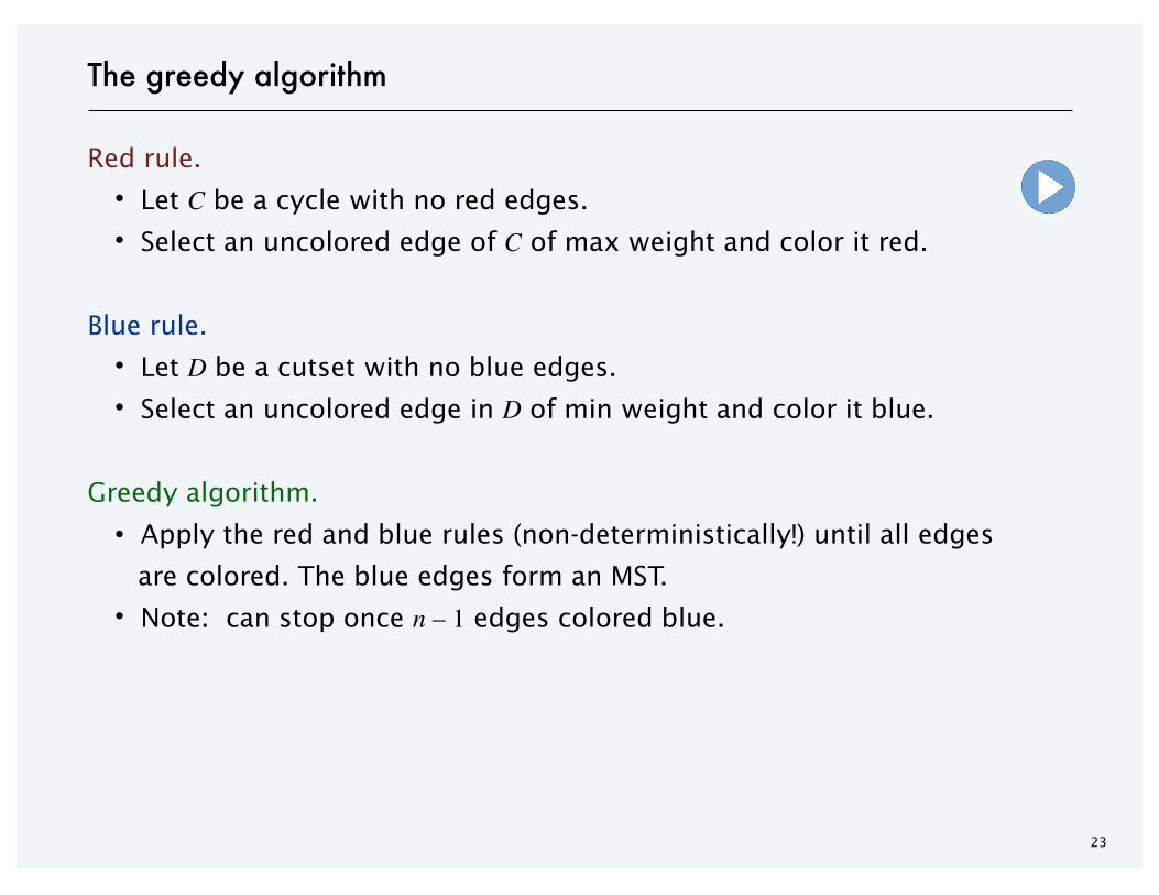
The greedy algorithm
Red rule.
・Let C be a cycle with no red edges.
・Select an uncolored edge of C of max weight and color it red.
Blue rule.
・Let D be a cutset with no blue edges.
・Select an uncolored edge in D of min weight and color it blue.
Greedy algorithm.
・Apply the red and blue rules (non-deterministically!) until all edges
are colored. The blue edges form an MST.
・Note: can stop once n – 1 edges colored blue.

24
Greedy algorithm: proof of correctness
Color invariant. There exists an MST T* containing all of the blue edges
and none of the red edges.
Pf. [by induction on number of iterations]
Base case. No edges colored ⇒ every MST satisfies invariant.
25
Greedy algorithm: proof of correctness
Color invariant. There exists an MST T* containing all of the blue edges
and none of the red edges.
Pf. [by induction on number of iterations]
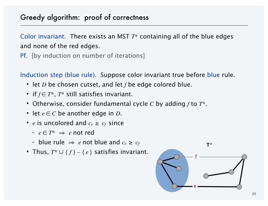
Induction step (blue rule). Suppose color invariant true before blue rule.
・let D be chosen cutset, and let f be edge colored blue.
・if f ∈ T*, T* still satisfies invariant.
・Otherwise, consider fundamental cycle C by adding f to T*.
・let e ∈ C be another edge in D.
・e is uncolored and ce ≥ cf since- e ∈ T* ⇒ e not red- blue rule ⇒ e not blue and ce ≥ cf
・Thus, T* ∪ { f } – { e } satisfies invariant.f
T*
e
26
Greedy algorithm: proof of correctness
Color invariant. There exists an MST T* containing all of the blue edges
and none of the red edges.
Pf. [by induction on number of iterations]
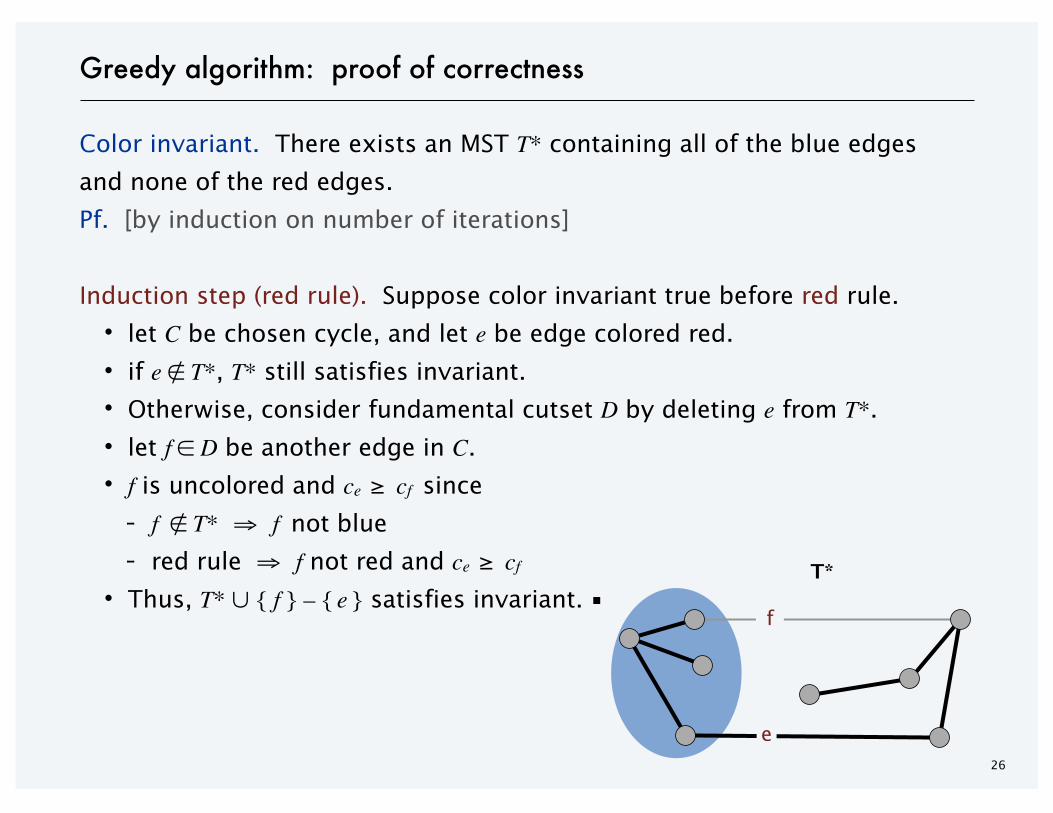
Induction step (red rule). Suppose color invariant true before red rule.
・let C be chosen cycle, and let e be edge colored red.
・if e ∉ T*, T* still satisfies invariant.
・Otherwise, consider fundamental cutset D by deleting e from T*.
・let f ∈ D be another edge in C.
・f is uncolored and ce ≥ cf since- f ∉ T* ⇒ f not blue- red rule ⇒ f not red and ce ≥ cf
・Thus, T* ∪ { f } – { e } satisfies invariant. ▪f
T*
e
27
Greedy algorithm: proof of correctness
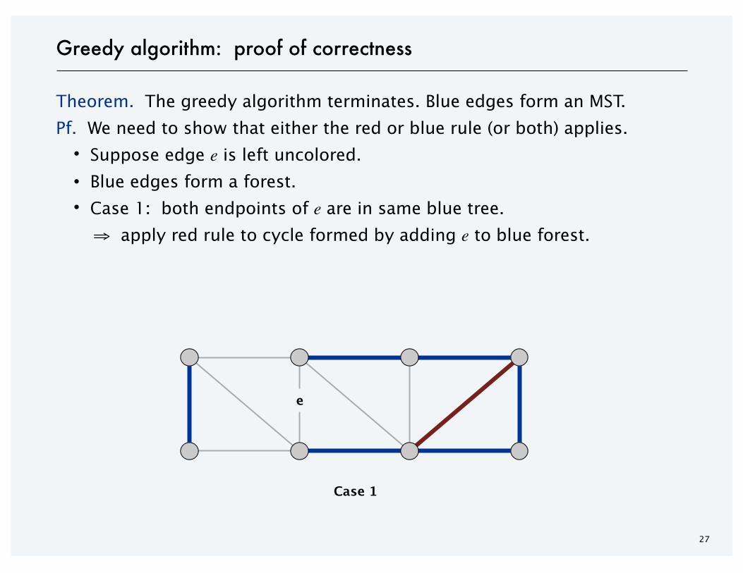
Theorem. The greedy algorithm terminates. Blue edges form an MST.
Pf. We need to show that either the red or blue rule (or both) applies.
・Suppose edge e is left uncolored.
・Blue edges form a forest.
・Case 1: both endpoints of e are in same blue tree.
⇒ apply red rule to cycle formed by adding e to blue forest.
Case 1
e

28
Greedy algorithm: proof of correctness
Theorem. The greedy algorithm terminates. Blue edges form an MST.
Pf. We need to show that either the red or blue rule (or both) applies.
・Suppose edge e is left uncolored.
・Blue edges form a forest.
・Case 1: both endpoints of e are in same blue tree.
⇒ apply red rule to cycle formed by adding e to blue forest.
・Case 2: both endpoints of e are in different blue trees.
⇒ apply blue rule to cutset induced by either of two blue trees. ▪
Case 2
e
4. GREEDY ALGORITHMS II
‣ Dijkstra's algorithm
‣ minimum spanning trees
‣ Prim, Kruskal, Boruvka
‣ single-link clustering
‣ min-cost arborescences
SECTION 6.2

30
Prim's algorithm
Initialize S = any node.
Repeat n – 1 times:
・Add to tree the min weight edge with one endpoint in S.
・Add new node to S.
Theorem. Prim's algorithm computes the MST.
Pf. Special case of greedy algorithm (blue rule repeatedly applied to S). ▪
S

31
Prim's algorithm: implementation
Theorem. Prim's algorithm can be implemented in O(m log n) time.
Pf. Implementation almost identical to Dijkstra's algorithm.
[ d(v) = weight of cheapest known edge between v and S ]
PRIM (V, E, c) _________________________________________________________________________________________________________________________________________________________________________________________________________________________________________________________________________________________________________________________________________________________________________________________________________________________________________________________________________________________________________________________________________________________________________________________________________________________________________________________________________________________________________________________________________________________________________________________________________________________________________________________________________________________________________________________________________________________________________________________________________________________________________________________________________________________________________________________________________________________________________________________________________________________________________________________
Create an empty priority queue.
s ← any node in V.
FOR EACH v ≠ s : d(v) ← ∞; d(s) ← 0.
FOR EACH v : insert v with key d(v) into priority queue.
WHILE (the priority queue is not empty)
u ← delete-min from priority queue.
FOR EACH edge (u, v) ∈ E incident to u:
IF d(v) > c(u, v)
decrease-key of v to c(u, v) in priority queue.
d(v) ← c(u, v)._________________________________________________________________________________________________________________________________________________________________________________________________________________________________________________________________________________________________________________________________________________________________________________________________________________________________________________________________________________________________________________________________________________________________________________________________________________________________________________________________________________________________________________________________________________________________________________________________________________________________________________________________________________________________________________________________________________________________________________________________________________________________________________________________________________________________________________________________________________________________________________________________________________________________________________________
32
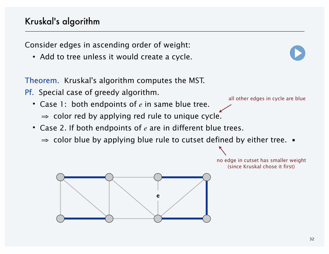
Kruskal's algorithm
Consider edges in ascending order of weight:
・Add to tree unless it would create a cycle.
Theorem. Kruskal's algorithm computes the MST.
Pf. Special case of greedy algorithm.
・Case 1: both endpoints of e in same blue tree.
⇒ color red by applying red rule to unique cycle.
・Case 2. If both endpoints of e are in different blue trees.
⇒ color blue by applying blue rule to cutset defined by either tree. ▪
e
all other edges in cycle are blue
no edge in cutset has smaller weight(since Kruskal chose it first)
33
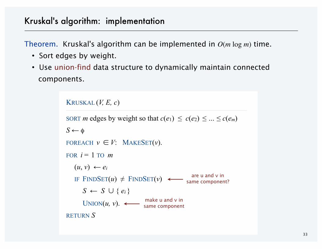
Kruskal's algorithm: implementation
Theorem. Kruskal's algorithm can be implemented in O(m log m) time.
・Sort edges by weight.
・Use union-find data structure to dynamically maintain connected
components.
KRUSKAL (V, E, c) ________________________________________________________________________________________________________________________________________________________________________________________________________________________________________________________________________________________________________________________________________________________________________________________________________________________________________________________________________________________________________________________________________________________________________________________________________________________________________________________________________________________________________________________________________________________________________________________________________________________________________________________________________________________________________________________________________________________________________________________________________________________________________________________________________________________________________________________________________________________________________________________________________________________________
SORT m edges by weight so that c(e1) ≤ c(e2) ≤ … ≤ c(em)S ← φ
FOREACH v ∈ V: MAKESET(v).
FOR i = 1 TO m(u, v) ← ei
IF FINDSET(u) ≠ FINDSET(v)S ← S ∪ { ei }
UNION(u, v).RETURN S________________________________________________________________________________________________________________________________________________________________________________________________________________________________________________________________________________________________________________________________________________________________________________________________________________________________________________________________________________________________________________________________________________________________________________________________________________________________________________________________________________________________________________________________________________________________________________________________________________________________________________________________________________________________________________________________________________________________________________________________________________________________________________________________________________________________________________________________________________________________________________________________________________________________
are u and v insame component?
make u and v insame component
34
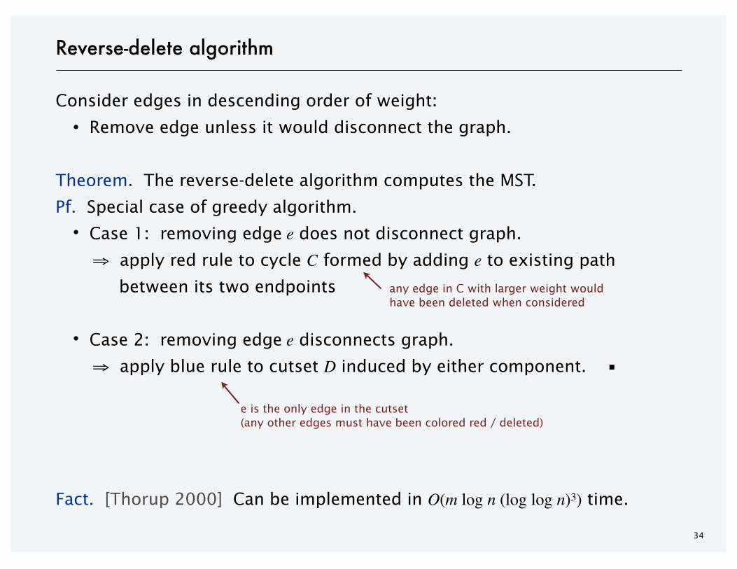
Reverse-delete algorithm
Consider edges in descending order of weight:
・Remove edge unless it would disconnect the graph.
Theorem. The reverse-delete algorithm computes the MST.
Pf. Special case of greedy algorithm.
・Case 1: removing edge e does not disconnect graph.
⇒ apply red rule to cycle C formed by adding e to existing path
between its two endpoints
・Case 2: removing edge e disconnects graph.
⇒ apply blue rule to cutset D induced by either component. ▪
Fact. [Thorup 2000] Can be implemented in O(m log n (log log n)3) time.
any edge in C with larger weight wouldhave been deleted when considered
e is the only edge in the cutset(any other edges must have been colored red / deleted)
35
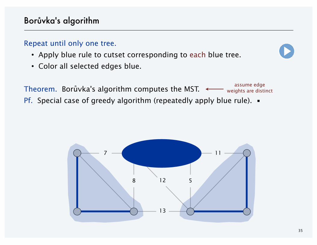
Borůvka's algorithm
Repeat until only one tree.
・Apply blue rule to cutset corresponding to each blue tree.
・Color all selected edges blue.
Theorem. Borůvka's algorithm computes the MST.
Pf. Special case of greedy algorithm (repeatedly apply blue rule). ▪
7 11
58 12
13
assume edgeweights are distinct
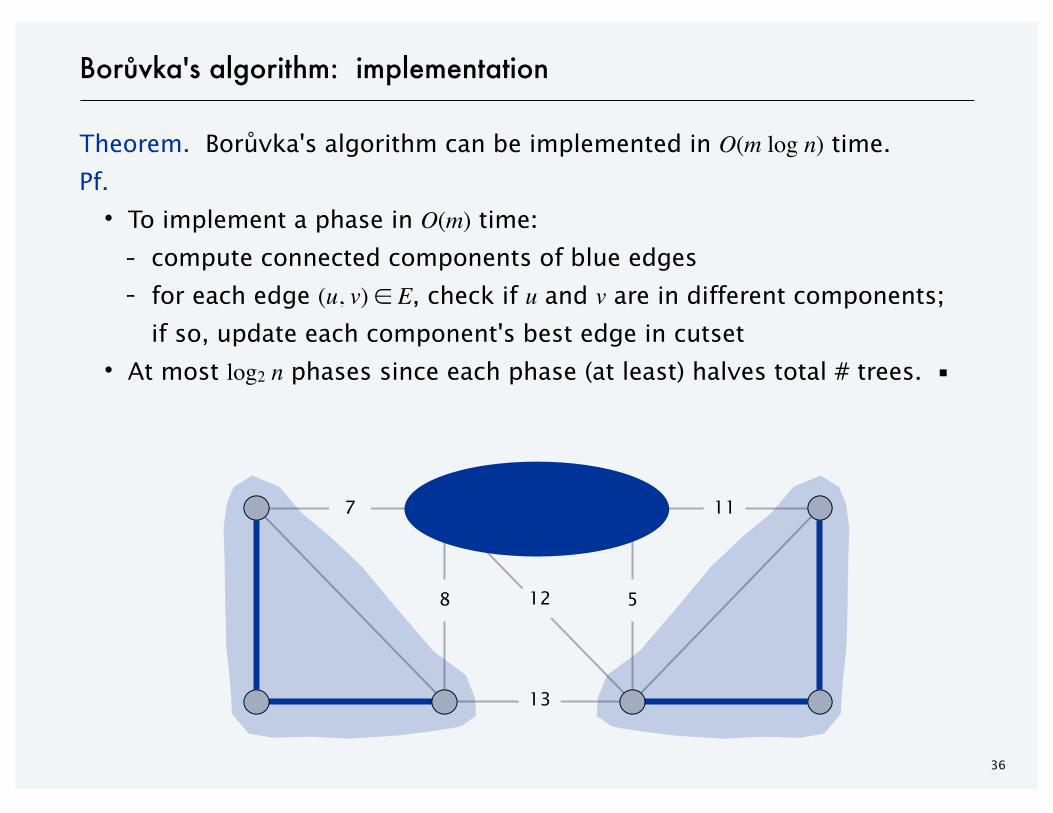
Theorem. Borůvka's algorithm can be implemented in O(m log n) time.
Pf.
・To implement a phase in O(m) time:
- compute connected components of blue edges- for each edge (u, v) ∈ E, check if u and v are in different components;
if so, update each component's best edge in cutset
・At most log2 n phases since each phase (at least) halves total # trees. ▪
36
Borůvka's algorithm: implementation
7 11
58 12
13

Edge contraction version.
・After each phase, contract each blue tree to a single supernode.
・Delete parallel edges, keeping only one with smallest weight.
・Borůvka phase becomes: take cheapest edge incident to each node.
37
Borůvka's algorithm: implementation
2 3
54 6
1 8
3 4 2
97
5
6 3
4 6
1
8
3 297
5
6
2, 5
3
4 6
1
8
3 297
5
2, 5
graph G contract edge (2 ,5)
delete parallel edges
1 1
1

Theorem. Borůvka's algorithm runs in O(n) time on planar graphs.
Pf.
・To implement a Borůvka phase in O(n) time:
- use contraction version of algorithm- in planar graphs, m ≤ 3n – 6.
- graph stays planar when we contract a blue tree
・Number of nodes (at least) halves.
・At most log2 n phases: cn + cn / 2 + cn / 4 + cn / 8 + … = O(n). ▪
38
Borůvka's algorithm on planar graphs
planar not planar

39
Borůvka-Prim algorithm
Borůvka-Prim algorithm.
・Run Borůvka (contraction version) for log2 log2 n phases.
・Run Prim on resulting, contracted graph.
Theorem. The Borůvka-Prim algorithm computes an MST and can be
implemented in O(m log log n) time.
Pf.
・Correctness: special case of the greedy algorithm.
・The log2 log2 n phases of Borůvka's algorithm take O(m log log n) time;
resulting graph has at most n / log2 n nodes and m edges.
・Prim's algorithm (using Fibonacci heaps) takes O(m + n) time on a
graph with n / log2 n nodes and m edges. ▪
O
�m +
n
log nlog
�n
log n
��

Remark 1. O(m) randomized MST algorithm. [Karger-Klein-Tarjan 1995]
Remark 2. O(m) MST verification algorithm. [Dixon-Rauch-Tarjan 1992]
40
deterministic compare-based MST algorithms
Does a linear-time MST algorithm exist?
year worst case discovered by
1975 O(m log log n) Yao
1976 O(m log log n) Cheriton-Tarjan
1984 O(m log*n) O(m + n log n) Fredman-Tarjan
1986 O(m log (log* n)) Gabow-Galil-Spencer-Tarjan
1997 O(m α(n) log α(n)) Chazelle
2000 O(m α(n)) Chazelle
2002 optimal Pettie-Ramachandran
20xx O(m) ???
SECTION 4.7
4. GREEDY ALGORITHMS II
‣ Dijkstra's algorithm
‣ minimum spanning trees
‣ Prim, Kruskal, Boruvka
‣ single-link clustering
‣ min-cost arborescences
42
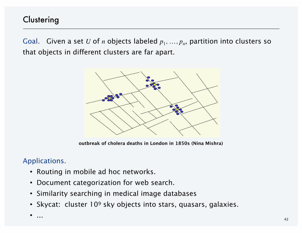
Goal. Given a set U of n objects labeled p1, …, pn, partition into clusters so
that objects in different clusters are far apart.
Applications.
・Routing in mobile ad hoc networks.
・Document categorization for web search.
・Similarity searching in medical image databases
・Skycat: cluster 109 sky objects into stars, quasars, galaxies.
・...
outbreak of cholera deaths in London in 1850s (Nina Mishra)
Clustering
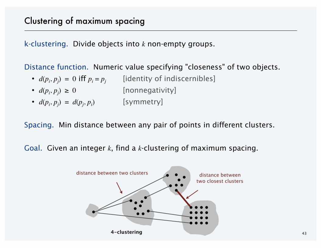
k-clustering. Divide objects into k non-empty groups.
Distance function. Numeric value specifying "closeness" of two objects.
・d(pi, pj) = 0 iff pi = pj [identity of indiscernibles]
・d(pi, pj) ≥ 0 [nonnegativity]
・d(pi, pj) = d(pj, pi) [symmetry]
Spacing. Min distance between any pair of points in different clusters.
Goal. Given an integer k, find a k-clustering of maximum spacing.
43
Clustering of maximum spacing
4-clustering
distance between two clusters distance betweentwo closest clusters
44
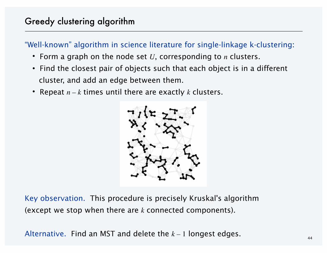
Greedy clustering algorithm
“Well-known” algorithm in science literature for single-linkage k-clustering:
・Form a graph on the node set U, corresponding to n clusters.
・Find the closest pair of objects such that each object is in a different
cluster, and add an edge between them.
・Repeat n – k times until there are exactly k clusters.
Key observation. This procedure is precisely Kruskal's algorithm
(except we stop when there are k connected components).
Alternative. Find an MST and delete the k – 1 longest edges.
Theorem. Let C* denote the clustering C*1, …, C*k formed by deleting the
k – 1 longest edges of an MST. Then, C* is a k-clustering of max spacing.
Pf. Let C denote some other clustering C1, …, Ck.
・The spacing of C* is the length d* of the (k – 1)st longest edge in MST.
・Let pi and pj be in the same cluster in C*, say C*r , but different clusters
in C, say Cs and Ct.
・Some edge (p, q) on pi – pj path in C*r spans two different clusters in C.
・Edge (p, q) has length ≤ d* since it wasn't deleted.
・Spacing of C is ≤ d* since p and q are in different clusters. ▪
45
Greedy clustering algorithm: analysis
p qpipj
Cs Ct
C*r
edges left after deletingk – 1 longest edges
from a MST

46
Tumors in similar tissues cluster together.
Reference: Botstein & Brown group
gene 1
gene n
gene expressed
gene not expressed
Dendrogram of cancers in human
SECTION 4.9
4. GREEDY ALGORITHMS II
‣ Dijkstra's algorithm
‣ minimum spanning trees
‣ Prim, Kruskal, Boruvka
‣ single-link clustering
‣ min-cost arborescences

48
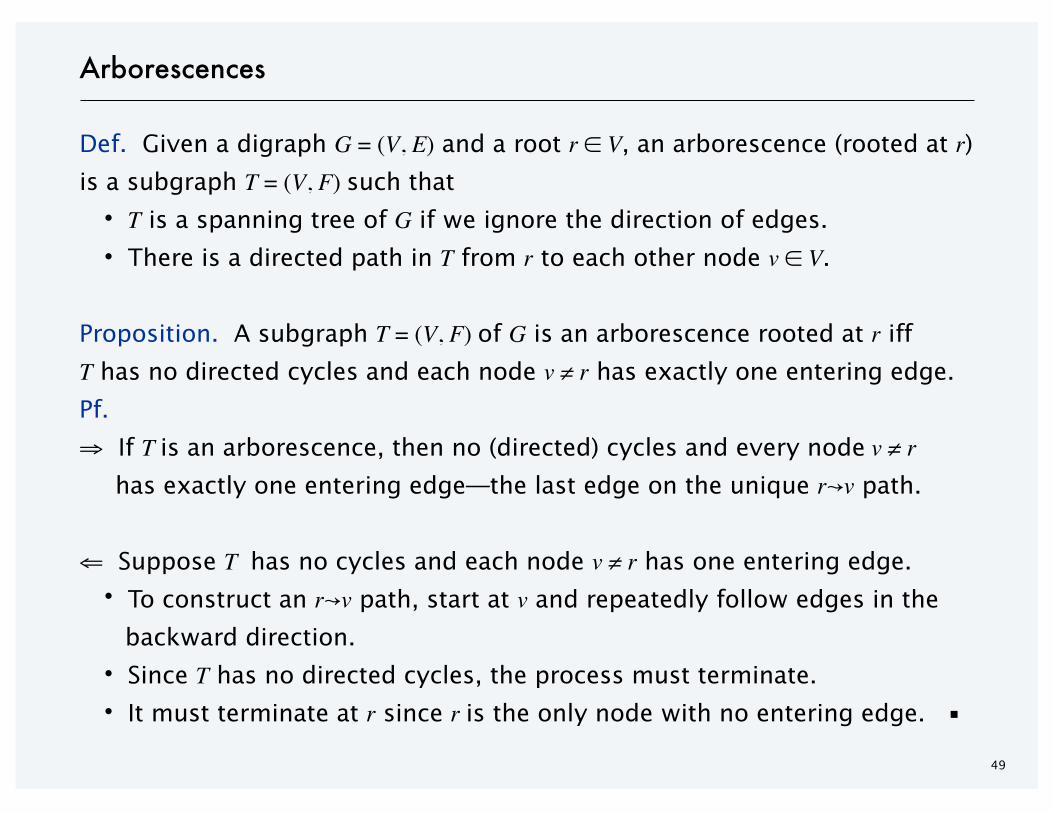
Def. Given a digraph G = (V, E) and a root r ∈ V, an arborescence (rooted at r) is a subgraph T = (V, F) such that
・T is a spanning tree of G if we ignore the direction of edges.
・There is a directed path in T from r to each other node v ∈ V.
Warmup. Given a digraph G, find an arborescence rooted at r (if one exists).
Algorithm. BFS or DFS from r is an arborescence (iff all nodes reachable).
Arborescences
r
49
Def. Given a digraph G = (V, E) and a root r ∈ V, an arborescence (rooted at r) is a subgraph T = (V, F) such that
・T is a spanning tree of G if we ignore the direction of edges.
・There is a directed path in T from r to each other node v ∈ V.
Proposition. A subgraph T = (V, F) of G is an arborescence rooted at r iffT has no directed cycles and each node v ≠ r has exactly one entering edge.
Pf.
⇒ If T is an arborescence, then no (directed) cycles and every node v ≠ r has exactly one entering edge—the last edge on the unique r↝v path.
⇐ Suppose T has no cycles and each node v ≠ r has one entering edge.
・To construct an r↝v path, start at v and repeatedly follow edges in the
backward direction.
・Since T has no directed cycles, the process must terminate.
・It must terminate at r since r is the only node with no entering edge. ▪
Arborescences

50
Problem. Given a digraph G with a root node r and with a nonnegative cost
ce ≥ 0 on each edge e, compute an arborescence rooted at r of minimum cost.
Assumption 1. G has an arborescence rooted at r.Assumption 2. No edge enters r (safe to delete since they won't help).
Min-cost arborescence problem
r
4
1
2
35
6
9
7
8
51
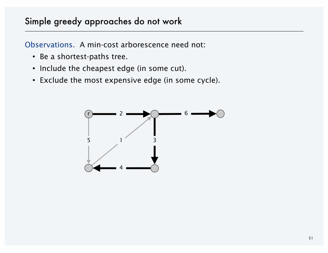
Observations. A min-cost arborescence need not:
・Be a shortest-paths tree.
・Include the cheapest edge (in some cut).
・Exclude the most expensive edge (in some cycle).
Simple greedy approaches do not work
r
4
1
2
35
6
52
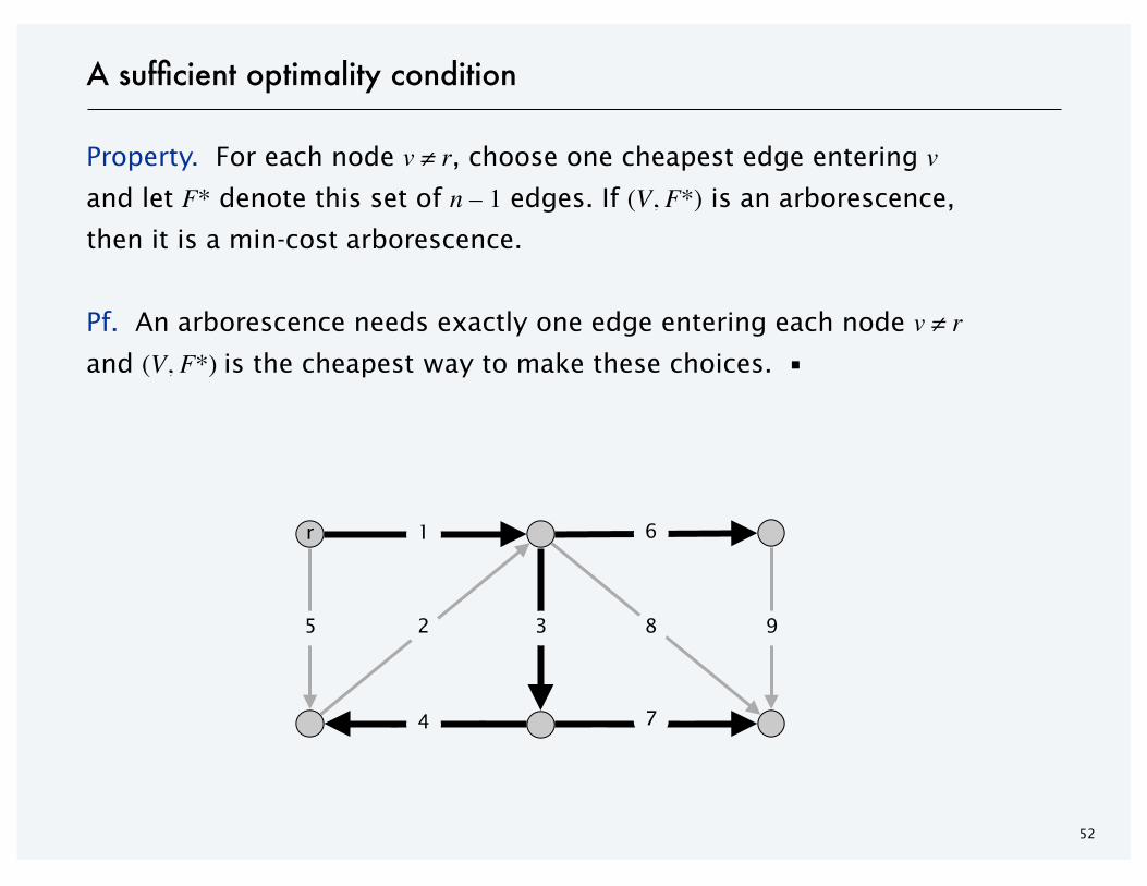
Property. For each node v ≠ r, choose one cheapest edge entering vand let F* denote this set of n – 1 edges. If (V, F*) is an arborescence,
then it is a min-cost arborescence.
Pf. An arborescence needs exactly one edge entering each node v ≠ rand (V, F*) is the cheapest way to make these choices. ▪
A sufficient optimality condition
r
4
2
1
35
6
9
7
8
53
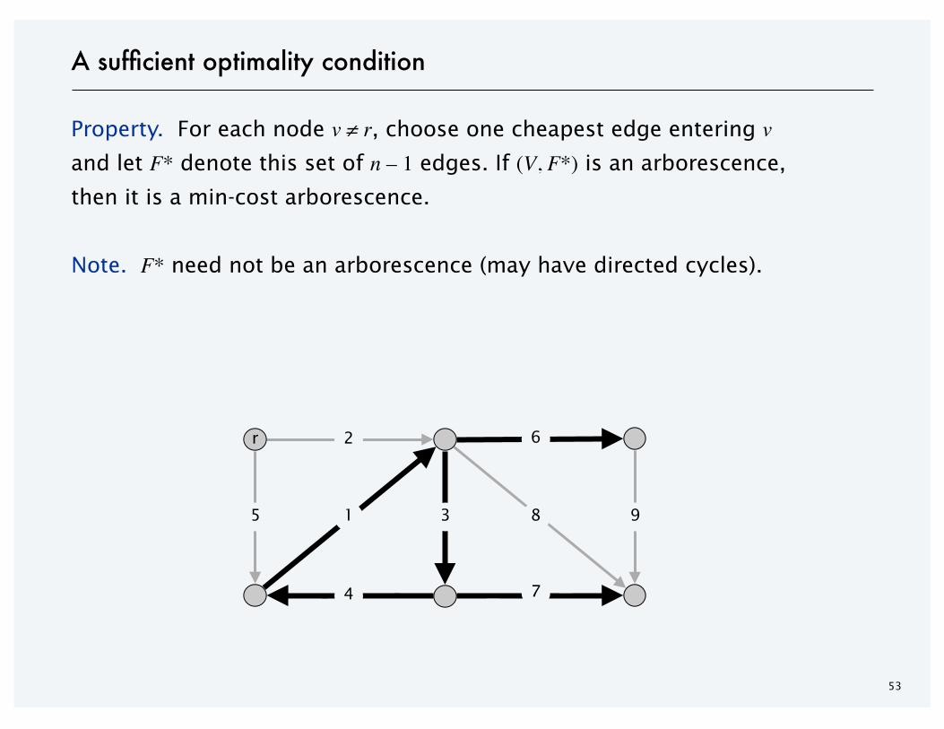
Property. For each node v ≠ r, choose one cheapest edge entering vand let F* denote this set of n – 1 edges. If (V, F*) is an arborescence,
then it is a min-cost arborescence.
Note. F* need not be an arborescence (may have directed cycles).
A sufficient optimality condition
r
4
1
2
35
6
9
7
8
54
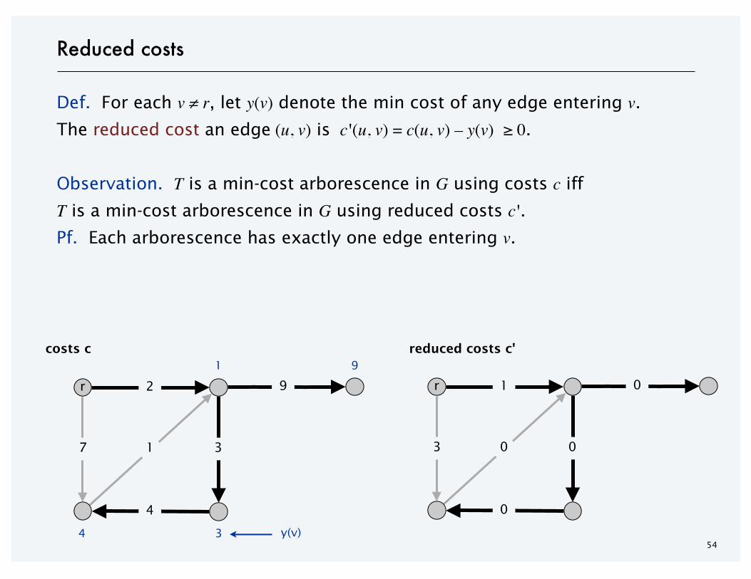
Def. For each v ≠ r, let y(v) denote the min cost of any edge entering v.The reduced cost an edge (u, v) is c'(u, v) = c(u, v) – y(v) ≥ 0.
Observation. T is a min-cost arborescence in G using costs c iffT is a min-cost arborescence in G using reduced costs c'.Pf. Each arborescence has exactly one edge entering v.
Reduced costs
r
4
1
2
37
9 r
0
0
1
03
0
costs c reduced costs c'1 9
4 3 y(v)

55
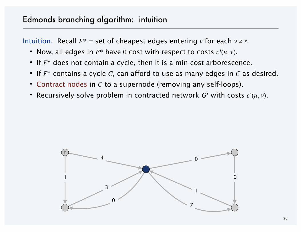
Intuition. Recall F* = set of cheapest edges entering v for each v ≠ r.
・Now, all edges in F* have 0 cost with respect to costs c'(u, v).
・If F* does not contain a cycle, then it is a min-cost arborescence.
・If F* contains a cycle C, can afford to use as many edges in C as desired.
・Contract nodes in C to a supernode.
・Recursively solve problem in contracted network G' with costs c'(u, v).
Edmonds branching algorithm: intuition
r
0
3
4
01
0
0
0
4 0
0
7
1
56
Intuition. Recall F* = set of cheapest edges entering v for each v ≠ r.
・Now, all edges in F* have 0 cost with respect to costs c'(u, v).
・If F* does not contain a cycle, then it is a min-cost arborescence.
・If F* contains a cycle C, can afford to use as many edges in C as desired.
・Contract nodes in C to a supernode (removing any self-loops).
・Recursively solve problem in contracted network G' with costs c'(u, v).
Edmonds branching algorithm: intuition
r
3
4
0
1
0
7
1
0

57
Edmonds branching algorithm
EDMONDSBRANCHING(G, r , c) _________________________________________________________________________________________________________________________________________________________________________________________________________________________________________________________________________________________________________________________________________________________________________________________________________________________________________________________________________________________________________________________________________________________________________________________________________________________________________________________________________________________________________________________________________________________________________________________________________________________________________________________________________________________________________________________________________________________________________________________________________________________________________________________________________________________________________________________________________________________________________________________________________________________________________________________________________________________________________________________________________________________________________________________________________________________________________________
FOREACH v ≠ r y(v) ← min cost of an edge entering v.c'(u, v) ← c'(u, v) – y(v) for each edge (u, v) entering v.
FOREACH v ≠ r: choose one 0-cost edge entering v and let F*be the resulting set of edges.IF F* forms an arborescence, RETURN T = (V, F*).ELSE
C ← directed cycle in F*.Contract C to a single supernode, yielding G' = (V', E').T' ← EDMONDSBRANCHING(G', r , c') Extend T' to an arborescence T in G by adding all but one edge of C.RETURN T.
_________________________________________________________________________________________________________________________________________________________________________________________________________________________________________________________________________________________________________________________________________________________________________________________________________________________________________________________________________________________________________________________________________________________________________________________________________________________________________________________________________________________________________________________________________________________________________________________________________________________________________________________________________________________________________________________________________________________________________________________________________________________________________________________________________________________________________________________________________________________________________________________________________________________________________________________________________________________________________________________________________________________________________________________________________________________________________________
58
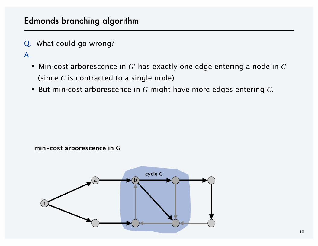
Q. What could go wrong?
A.
・Min-cost arborescence in G' has exactly one edge entering a node in C(since C is contracted to a single node)
・But min-cost arborescence in G might have more edges entering C.
Edmonds branching algorithm
ba
r
cycle C
min-cost arborescence in G
59
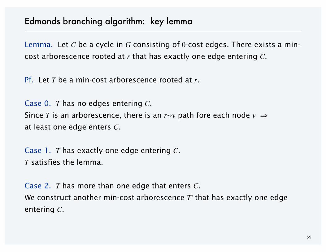
Lemma. Let C be a cycle in G consisting of 0-cost edges. There exists a min-
cost arborescence rooted at r that has exactly one edge entering C.
Pf. Let T be a min-cost arborescence rooted at r.
Case 0. T has no edges entering C.
Since T is an arborescence, there is an r↝v path fore each node v ⇒at least one edge enters C.
Case 1. T has exactly one edge entering C.
T satisfies the lemma.
Case 2. T has more than one edge that enters C.
We construct another min-cost arborescence T' that has exactly one edge
entering C.
Edmonds branching algorithm: key lemma

Case 2 construction of T'.
・Let (a, b) be an edge in T entering C that lies on a shortest path from r.
・We delete all edges of T that enter a node in C except (a, b).
・We add in all edges of C except the one that enters b.
b
60
Edmonds branching algorithm: key lemma
a
r
cycle CT
path from r to C usesonly one node in C

T
Case 2 construction of T'.
・Let (a, b) be an edge in T entering C that lies on a shortest path from r.
・We delete all edges of T that enter a node in C except (a, b).
・We add in all edges of C except the one that enters b.
Claim. T' is a min-cost arborescence.
・The cost of T' is at most that of T since we add only 0-cost edges.
・T' has exactly one edge entering each node v ≠ r.
・T' has no directed cycles.
(T had no cycles before; no cycles within C; now only (a, b) enters C)
b
61
Edmonds branching algorithm: key lemma
ba
T is an arborescence rooted at r
r
cycle CT'
path from r to C usesonly one node in C
and the only path in T' to a is the path from r to a
(since any path must follow unique entering
edge back to r)

Theorem. [Chu-Liu 1965, Edmonds 1967] The greedy algorithm finds a
min-cost arborescence.
Pf. [by induction on number of nodes in G]
・If the edges of F* form an arborescence, then min-cost arborescence.
・Otherwise, we use reduced costs, which is equivalent.
・After contracting a 0-cost cycle C to obtain a smaller graph G',the algorithm finds a min-cost arborescence T' in G' (by induction).
・Key lemma: there exists a min-cost arborescence T in G that
corresponds to T'. ▪
Theorem. The greedy algorithm can be implemented in O(m n) time.
Pf.
・At most n contractions (since each reduces the number of nodes).
・Finding and contracting the cycle C takes O(m) time.
・Transforming T' into T takes O(m) time. ▪
62
Edmonds branching algorithm: analysis

Theorem. [Gabow-Galil-Spencer-Tarjan 1985] There exists an O(m + n log n) time algorithm to compute a min-cost arborescence.
63
Min-cost arborescence
Related Documents


![Seam Carving A - 國立臺灣大學disp.ee.ntu.edu.tw/~pujols/CSVT.pdf · The seam carving algorithm, proposed by Avidan et al. [1], is also a popular method for image retargeting.](https://static.cupdf.com/doc/110x72/60a3c8a94930654c77755b1e/seam-carving-a-oececdispeentuedutwpujolscsvtpdf-the-seam.jpg)


![Seam Carving with Forward Gradient Difference Maps · The seam carving [2] is a simple contents-aware image resizing technique, which is composed of the following three steps: •](https://static.cupdf.com/doc/110x72/60a3c8a94930654c77755b1d/seam-carving-with-forward-gradient-difference-maps-the-seam-carving-2-is-a-simple.jpg)
