4. Estimating the Distribution of Wet-Day Amounts for … 4 4. Estimating the Distribution of Wet-Day Amounts for Areal Rainfall Using the Gamma Distribution Contents 4.1. Introduction

Chapter 4

4. Estimating the Distribution of Wet-Day Amounts for Areal Rainfall

Using the Gamma Distribution

Contents

4.1. Introduction.................................................................................................................. 90

4.2. The Gamma Distribution and Point and Areal Rainfall. ......................................... 91

4.2.1. Introduction to the Gamma Distribution.............................................................. 91

4.2.2. Fitting the Gamma Distribution to Daily Rainfall Data....................................... 93

4.2.3. Testing Goodness-of-Fit of the Gamma Distribution for Point and Areal Rainfall

95

4.3. Development of Methodology ................................................................................... 105

4.3.1. Spatial Dependence Between Wet-Day Values................................................. 106

4.3.2. Empirical Relationships Between Single-Station and n-Station Timeseries ..... 108

4.3.3. Estimation of n-Station-Mean Scale Parameter (βn) .......................................... 111

4.3.4. Estimation of n-Station-Mean Shape Parameter (αn)......................................... 114

4.3.5. Summary............................................................................................................ 123

4.4. Application of Methodology to the Estimation of Gamma Parameters of ‘True’

Areal Mean Precipitation...................................................................................................... 124

4.4.1. Extension of Methodology to the Estimation of Gamma Parameters of the ‘True’

Areal Mean .......................................................................................................................... 124

4.4.2. Estimated Gamma Parameters for ‘True’ Areal Mean ...................................... 130

4.4.3. Additional Uncertainty in Estimates of αN and βN for Small Values of n .......... 133

4.5. Estimating Distribution Extremes Using the Gamma Parameters ....................... 137

4.5.1. Assessment of Goodness-of-Fit at Distribution Tails........................................ 137

4.5.2. Estimating Percentile Values from the Gamma Distribution............................. 139

4.6. Discussion and Summary .......................................................................................... 142

90

4.1. Introduction

The objective of this chapter is to develop and test a technique for estimating the distribution of

wet-day areal rainfall amounts for a grid box, which requires only a limited number of stations.

As has been demonstrated in the previous chapter for the dry-day probability of daily rainfall

timeseries, it is expected that the approach developed will be suitable for application to the

quantitative assessment of climate model performance for any region of the world, even where

only a sparse station network is available.

Similarly to the approach taken in Chapter 3 for the dry-day probability, a method is initially

developed using three station datasets from UK, China and Zimbabwe, for estimating the

statistical parameters of the average of a number (n) of individual precipitation records. This

approach is then extended to the estimation of those parameters of the ‘true’ areal mean for a

region, which would include an infinite number of stations, N. The approach taken here also

makes use of relationships between point and areal scale rainfall, using the spatial dependence

between stations in a region.

This section will begin with a brief introduction to the gamma distribution and its application to

daily rainfall, and a demonstration that it is an appropriate distribution for both point and areal

rainfall wet-day amounts (Section 4.2). A methodology for estimating the parameters of the

gamma distribution for an n-station average series is developed and tested in Section 4.3 and then

this method is extended to the estimation of the parameters of an average series that is

representative of a ‘true’ areal mean (Section 4.4). The methodology and its application are

reviewed and discussed in Section 4.5.

Chapter 4: Estimating the Distribution of Wet-day Amounts for Areal Rainfall using the Gamma Distribution

91

4.2. The Gamma Distribution and Point and Areal Rainfall.

4.2.1. Introduction to the Gamma Distribution

The gamma distribution is often used to model the distribution of wet-day rainfall amounts (e.g

Groisman et al., 1999; Semenov and Bengtsson, 2002; Wilby and Wigley, 2002; Watterson and

Dix, 2003). Unlike the symmetrical Gaussian (Normal) distribution, the gamma distribution is

distinctly skewed to the right, which suits the distribution of daily rainfall and accommodates the

lower limit of zero which constrains rainfall values (Wilks, 2006).

Other distributions that have been used to model the distribution of wet-day rainfall amounts

include the Weibull distribution (e.g. Boulanger et al., 2007) the log-normal (e.g. Shoji and

Kitaura, 2006) and the mixed exponential distribution (e.g. Wilks, 1999b). Studies that have

compared the suitability of two or more different distributions such as Boulanger et al. (2007)

have found that no single distribution consistently suits all regions, seasons and climates better

than others. Whilst Wilks (1999), for example, found that the gamma distribution generally fitted

the least well for daily rainfall in the United States and the mixed exponential was more

appropriate, Gregory et al. (1993) tested a similar range of models for UK rainfall and found that

the gamma distribution performed best for most regions and seasons.

The gamma distribution is defined by two parameters; the shape (α) and scale (β) parameters, in

the following formula:

)(

)/exp()/()(

1

αβ

ββ α

Γ

−=

−xx

xf ,

Equation 4-1

where Γ(α) is a value of the standard mathematical function called the gamma function and is

defined by:

92

∫∞

−−=Γ0

1)( dtettαα

Equation 4-2

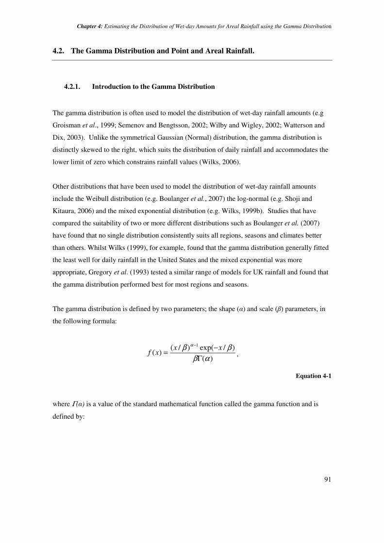
The shape parameter (α) essentially determines the level of positive skew (Figure 4-1, Left). This

value is always greater than 0, and for α < , the gamma distribution is very strongly skewed to the

right, and for the particular case of α=1, the distribution is exponential. When greater α > 1, the

shape of the distribution alters to approach the y-axis at the origin. The scale parameter (β)

determines the spread of values, stretching or squeezing the distribution when large or small,

respectively (Figure 4-1, Right).

Figure 4-1: Gamma distribution frequency distributions for a different values of the shape

parameter, α when scale parameter, β, is kept constant at 1 (left) and for values of the scale

parameter , β, when shape parameter α is kept constant at 2 (right).

The product of the shape and scale parameters (αβ) gives the mean of the distribution. As we are

dealing with the distribution of wet-day values only, this gives the mean wet-day amount, not the

mean daily amount. The distribution variance is given by αβ2 (Wilks, 2006).

α = 0.5

α = 2

α = 3

α = 4

α = 1

β = 0.5

β = 1

β =2

β = 5 β = 10


93

4.2.2. Fitting the Gamma Distribution to Daily Rainfall Data

The gamma distribution is fitted to the station and areal-average daily time series using an

analytical approximation to the maximum-likelihood technique. Wilks (2006) discusses the

advantages of this technique over the alternative approach of moment estimation. Whist the latter

is a more simple technique, it can be described as ‘inefficient’ as it does not make use of all the

distribution information available and the moments of the data may not correspond exactly to the

moments of its distribution. The method of moments can also give particularly bad results for

cases where the shape parameter is very low (Wilks, 2006), and because the shape parameter for

station precipitation data tends to be less than 1, the method of moments is avoided here.

The Thom (1958) approximation for the Maximum Likelihood is used here. The maximum

likelihood approach uses the concept that the ‘likelihood’ is a measure of the degree to which the

data support particular values of the parameters (Wilks, 2006). The Thom estimator for the shape

parameter is:

D

D

4

3/411 ++=α

Equation 4-3

Where the sample statistic, D, is the difference between the natural log of the sample mean and

the mean of the logs of the data.

∑=

−=n

i

ixn

xD1

)ln(1

)ln(

Equation 4-4

The gamma distribution is fitted to wet day values only (values on days where rainfall amount is

greater than or equal to 0.3mm), which means that the actual distribution of values provided to

the fitting procedure is truncated at this value. Whilst the 0.3mm threshold is necessary to

account for the limited precision of station records (see Section 3.3.1 for discussion of the choice

of threshold), it creates a difficulty in fitting the distribution because the gamma parameters are

94

chosen to give the best fit to a set of data that has no values between 0.0 and 0.3. The fitting

procedure tends to incorrectly favour higher values of the shape parameter than are appropriate

for the values above 0.3mm because α > 1 forces the distribution close to the origin at x=0. These

poorly fitting distributions also tend to underestimate the height of the data histogram’s peak

which normally occurs at, or close to, 0.3 mm (see Figure 4-2, left). The disparity occurs because

the fitting regime assumes that there are no values between 0 and 0.3mm, when actually, there are

an unknown number of values. The frequency of values between 0 and 0.3 mm should therefore

be treated as ‘unknown’ when the curve is fitted, rather than zero.

This is dealt with by subtracting 0.25 mm from each wet-day value to fit a shifted distribution

with the lowest values at 0.05 mm (the values are not shifted back to 0 mm by subtracting 0.3 mm

as this would leave a high proportion of zero values which would then be excluded from the fitted

distribution).

A shifted gamma distribution such as this is sometimes called the ‘Pearson Type III distribution’,

whereby the third parameter, the shift parameter, ζ, is included in the function (Equation 4-5). In

this application the shift parameter, ζ,, is known to be 0.25 (Wilks, 2006). Alternative approaches

to dealing with a truncated distribution such as this are demonstrated by Koning and Franses

(2005) and Wilks (1990).

)(

)/)(exp()/)(()(

1

αβ

βζβζ α

Γ

−−−=

−xx

xf

Equation 4-5


95

Figure 4-2: Example of the Gamma distribution fitted to (left) wet day values, and (right) to wet-day

values-0.25.

This ‘shifted’ distribution gives a much better fit to the data in the example in Figure 4-2. Most

notably, this is because it fits a shape parameter lower than 1.0, the threshold at which the shape

of the distribution changes such that zero values occur with greater frequency than zero.

4.2.3. Testing Goodness-of-Fit of the Gamma Distribution for Point and Areal

Rainfall

While the gamma distribution has been used frequently in previous studies to model both point

and areal daily rainfall amounts (e.g Groisman et al. 1999; Semenov and Bengtsson, 2002; Wilby

and Wigley, 2002; Watterson and Dix, 2003), there are also studies which suggest that the gamma

distribution does not provide an appropriate fit to daily precipitation data (Koning and Franses,

2005). Koning and Franses (2005) claim that the gamma distribution does not provide a good fit

to daily precipitation values because the fit is too heavily weighted towards the lower and more

frequently occurring values of the distribution, leading to poor fit (usually in the form of over-

estimation) at the upper-extremes. It is therefore prudent to assess how well the distribution fits

the data used here before applying it in this research.

96

4.2.3.1. Goodness-of-Fit Test Methods

The goodness-of-fit can be tested both qualitatively, by visual comparison of the data with the

distribution, and also quantitatively. The quantitative test most often used is the Lillefors test, a

variation on the Kolmogorov-Smirnov test used for testing the fit of a distribution when the test

is being conducted using the same data that were used to fit the distribution (Wilks, 2006). This

test compares the Dn test statistic (the largest difference, in absolute value, between the empirical

and fitted cumulative distribution functions) with a critical value determined by the number of

observations in the dataset and the chosen significance level (Wilks, 2006).

Qualitative fit-tests used often include simple plots of the data histogram with the fitted

distribution overlaid, and Quantile-Quantile (‘Q-Q’) plots and Percentile-Percentile (‘P-P’) plots.

Q-Q plots show the quantile values of each observed data value versus the theoretical value for

that quantile sorted into ascending order of observed values. A good fit will closely follow the

line x=y. Interpretation of Q-Q plots can be biased towards the highest extremes of the

distribution which are more dominant on the graph due to their high values, whilst the smaller,

but more numerous values are compacted into the lower corner of the graph. The 90%, 95% and

99% quantile values, therefore, are marked on all the Q-Q plots shown here for the purposes of

(a) illustrating the proportion of the graph which represents this portion of the data, and (b)

because the fit to the tail of the distribution is particularly important if the distribution is to be

used for estimating extremes later on. P-P plots show the values of the theoretical cumulative

distribution function (CDF) compared with the observed CDF. This gives a more balanced

impression of how well the fitted distribution represents the data across the whole distribution.

A sample of 20 stations from each of the three study regions is used to test the fit of the gamma

distribution to station data, and 20 randomly selected n-station average series’, and all of the tests

mentioned above are used. The rainfall data used are accurate to one decimal place, and this

causes a block or step effect in the deviations plotting in the P-P plot, which results in a larger

maximum Dn value than would occur in the data if they were given to a higher degree of

accuracy. Additional decimal places are therefore added to the data for the purposes of these tests

using uniformly distributed random values. The effect of this adjustment can be seen in Figure

4-3, particularly for the lowest probability values where the graph is particularly blocky. In most

cases, the addition of decimal places reduces the Dn value, and in the second example in Figure

4-3, this is enough to alter the result of the test.


97

Figure 4-3: PP plots, with Dn values, and Lillefors test results, for two stations based on original data

to 1 decimal place (left) and the for same stations but with uniform randomly selected additional

decimal places (right).

4.2.3.2. Goodness-of-Fit Test Results for Point Rainfall

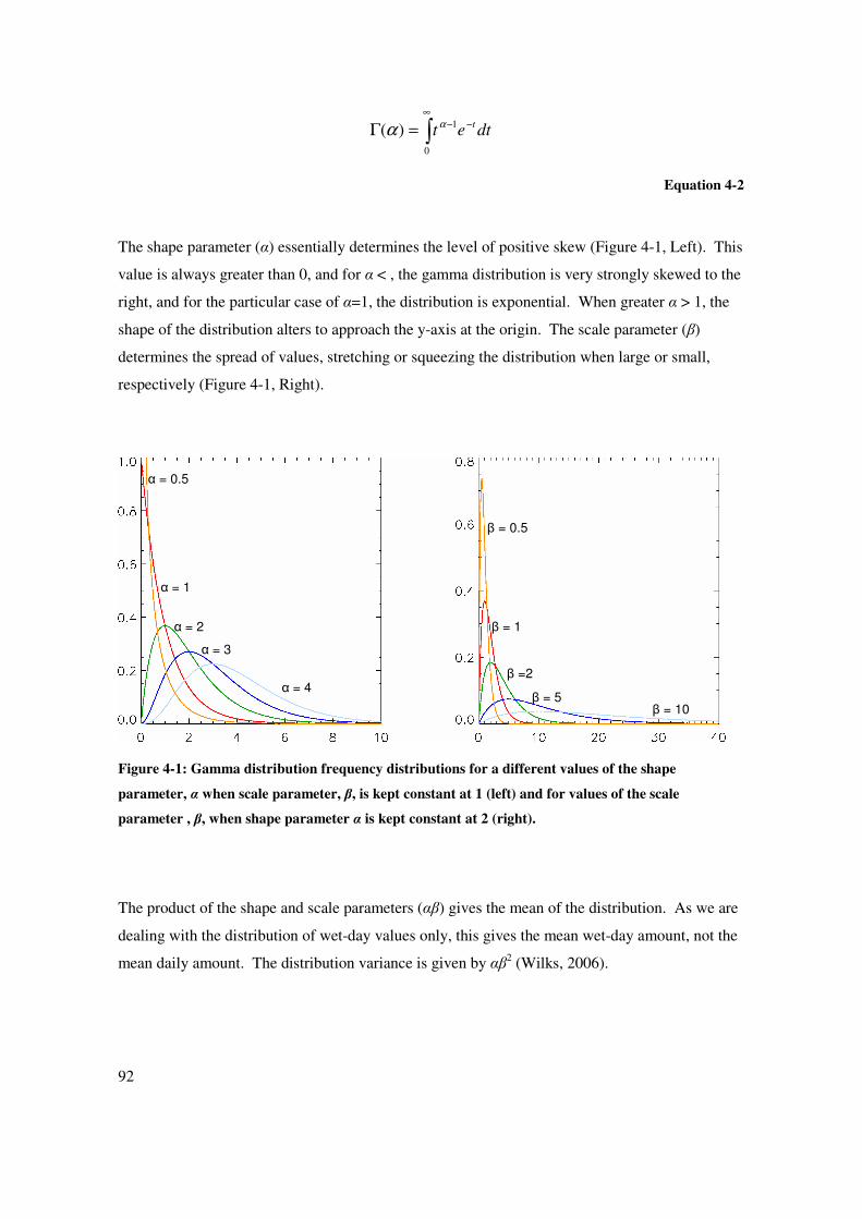
The plotted histograms demonstrate an overall good fit to the data (Figure 4-4, Figure 4-5 and

Figure 4-6). The exceptions to this are the cases where the number of data points is small (less

than 100), and this can be seen in Figure 4-6 for Zimbabwe where JJA is the dry season and there

are fewer wet days on which to fit the distribution. The results of the Lillefors test, however,

suggest that in most cases, the data differs significantly from the fitted distribution at the 90%

, 95%

and 99% level, and therefore the gamma distribution does not provide a good fit. The cases

98

where the Lillefors test does not indicate a poor fit, are few, and often those which are based on

small sample sizes, and therefore appear to fit the least well when the histograms are studied.

The result of this test is heavily influenced by the sample size, which determines the critical value

used. When the sample size is large the data values are expected to more closely follow the

gamma distribution, such that as the number of data points approaches infinity, it approaches a

perfect gamma distribution. This means that because the sample sizes used here are large (more

than 1000), it is expected that they will very closely follow the gamma distribution and the test

tends to fail, even though the data plots shown in Figure 4-4, Figure 4-5 and Figure 4-6 suggest a

relatively good fit to the data. The percentile values indicated on the Q-Q plots also indicate how

well the distribution fits the data at the tail of the distribution, and indicates that the fitted

distribution tends to underestimate the extremes of the distribution, but generally fits well up to

the 95th percentile.

While the gamma distribution may not provide a fit that is statistically significant, for the

purposes of this research, the approximation to the gamma distribution that the fitted parameters

give is good enough to represent the general form of the data which is all that is required here.


99

Figure 4-4: Goodness of fit test plots gamma distribution to JJA and DJF wet-day rainfall amounts

for an example station in UK. From left to right: Histogram, Q-Q plot (with 90th

, 95th

and 99th

percentile values marked), and P-P plot.

100


for an example station in China. From left to right: Histogram, Q-Q plot (with 90th

, 95th

and 99th



101


for an example station in Zimbabwe. From left to right: Histogram, Q-Q plot (with 90th

, 95th

and 99th


4.2.3.3. Goodness-of-Fit Test Results for Areal Rainfall

The distribution of daily rainfall values alters in shape as series are averaged, with the variance

becoming reduced and the skewness becoming less as the distribution becomes more ‘normal’.

It is therefore wise to test the fit of the gamma distribution to n-station average series’ as well as

to individual stations.

Randomly selected clusters of n stations are selected, averaged, and tested using the same

methods as for point rainfall above. This is done by selecting a box of a random size (limited to a

maximum 2.5 degrees latitude and longitude in size) and position (latitude and longitude of the

bottom left hand corner), and using the stations available within that box to create an average

series. The average series is created by averaging values at all stations for each day. Any day

102

which is missing a data value at any station is not included in the average series to avoid

producing, for example, a 10 station series, which for some days only contains data from 5 days

or 8 days, and ensures a true ‘n-station’ average series, albeit with a relatively large number of

missing data days. This provides a sample of areal-average series for each region which covers a

range of gauge densities and spatial resolutions. Again, 20 such samples are randomly selected

from each region but only an example is shown here (Figure 4-7, Figure 4-8 and Figure 4-9).

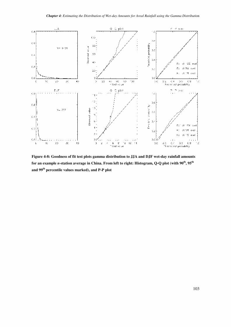
On the whole, the distribution shows a good fit when the histogram, Q-Q and P-P plots are

assessed. Some examples give a poor fit, but again this tends to be due to small sample size. The

number of valid data points becomes fewer as the number of stations included increases as the

chance of all stations containing real data becomes less. This is more of a problem for drier

regions and seasons (notably JJA in Zimbabwe and DJF in China) where there are fewest wet

days to which to fit the distribution.


for an example n-station average in UK. From left to right: Histogram, Q-Q plot (with 90th

, 95th

and

99th



103


for an example n-station average in China. From left to right: Histogram, Q-Q plot (with 90th

, 95th

and 99th

percentile values marked), and P-P plot

104


for an example n-station average in Zimbabwe. From left to right: Histogram, Q-Q plot (with 90th

,

95th

and 99th

percentile values marked), and P-P plot

.


105

4.3. Development of Methodology

In the previous chapter, it was shown that it is possible to make use of simple laws of probability,

together with the concept of ‘effective n’ , determined by a measure of spatial dependence

between stations, to estimate the dry day probability of any ‘n’ station mean. In this case,

however, such a convenient semi-theoretical relationship is not available so an empirical

approach is employed.

If it is assumed that the shape parameter (αn) of the n-station average series is related to the mean

shape parameter of the individual stations ( ni,α ) by an empirically determined function f1(x),

then:

)( ,1 nin f αα = .

Equation 4-6

Similarly:

)( ,2 nin f ββ = ’

Equation 4-7

where, f2(x) is a function by which the scale parameter (βn) of an n-station average series is

related to the mean scale parameter of all n stations ( ni ,β ) which contribute to the n-station mean.

The shape and scale parameters of the gamma distribution are known to be related, such that their

product gives the distribution mean.

αβ=x

Equation 4-8

This means that both parameters need not to be empirically predictable as long as we know the

distribution mean. The distribution mean is the Mean Wet-Day Amount (MWDA) and can be

estimated by the mean daily rainfall (MD) divided by the probability of a wet-day, hence:

106

])(1[ n

n

ndP

MDMWDA

−=

Equation 4-9

where x

MDn can be determined easily because the mean daily rainfall in an n-station average is, of

course, equal to the average of all mean rainfalls in the n individual stations ( niMD , ); and P(d)n

is calculated for the n-station average series using the methodology described in Chapter 3.

It can reasonably be expected that the functions f1(x) and f2(x), which relate the station parameters

to the n-station mean parameters, will depend to some extent on the degree of spatial dependence

between the stations, and the number of stations that are available.

4.3.1. Spatial Dependence Between Wet-Day Values

In Chapter 3 (Section 3.3.3), it was noted that the correlation coefficient, r, was not the most

appropriate measure of spatial dependence when dealing only with wet or dry day occurrences.

In this case, it is only the correlation between wet-day amounts that is of interest. It seems

appropriate therefore, to remove any day for which both stations in a pair are dry before

calculating the correlation between the station timeseries. Excluding those days where zero

values are registered at both stations can be expected to result in a lower correlation between the

two stations than would be obtained if coincident dry days were not removed. This is

demonstrated in Figure 4-10, Figure 4-11, and Figure 4-12, where r(wet) values are consistently

lower than r(all).


107

Figure 4-10: Comparison of ‘r’ with ‘r(wet)’ for randomly selected station pairs from the UK data

set.

Figure 4-11 Comparison of ‘r’ with ‘r(wet)’ for randomly selected station pairs from the

Zimbabwean data set.

108

Figure 4-12 Comparison of ‘r’ with ‘r(wet)’ for randomly selected station pairs from the Chinese data

set.

4.3.2. Empirical Relationships Between Single-Station and n-Station Timeseries

The functions f1(x) and f2(x) are expected to involve terms n and r(wet). While it may be possible

to fit these functions using both terms, the relationship can be simplified by consolidating these

two terms into one, again using the concept of effective independent sample size, where the n’

formula is modified to use r(wet). This application of ‘Effective n’ as a scaling factor which

encompasses the level of spatial variability and the station density in a region, allows the use of

data from all three regions, and for all four seasons, thus providing relationships that might be

universal to any region, season or climatic regime, regardless of the density of the available

station network. In the following analysis, data from UK, China and Zimbabwe are used

together, in order to seek universal empirical relationships. This is done using randomly selected

samples of n stations from all three datasets (UK, China and Zimbabwe, datasets described in

Section 3.4.1). For each sample, n′ is calculated and plotted against the ratio of the n-station

parameters (αn and βn) to the mean single-station parameters ( ni,α and ni ,β ) in order to identify

any useful relationships (Figure 4-13 and Figure 4-14).


109

In the case of the scale parameter (Figure 4-13), the two variables appear to be very strongly

related. However, for the shape parameter (Figure 4-14), the relationships between the variables

appear to vary systematically with region, which does not suit our requirement that any

relationship should be universal so that it can be applied in any region of the world.

Figure 4-13: Ratio of n-station to mean single-station β vs effective n (n’) for randomly selected

sample clusters of n stations from the UK (Blue), Zimbabwean (Green) and Chinese (Red) station

data sets. Plot symbols indicate different seasons: ◊= MAM, =JJA, ∆∆∆∆=SON, x=DJF.

110

Figure 4-14: Ratio of n-station to mean single-station α vs effective n (n’) for randomly selected

clusters of n stations from the UK (Blue), Zimbabwean (Green) and Chinese (Red) station data sets.

Plot symbols indicate different seasons: ◊= MAM, =JJA, ∆∆∆∆=SON, x=DJF.

The shape parameter of the distribution of daily rainfall is known to be more stable in space and

time than the scale parameter (Groisman et al., 1999). Alteration of the shape parameter with

spatial averaging is relatively minor, with values typically increasing from 0.75 to around 1.0.

While the alteration from a <1 shape parameter to >1 makes a significant alteration to the

distribution shape because it marks the shift from an exponential shape to one that begins at the

origin (see Figure 4-1, left for illustration) these small variations in the values are more likely to

be obscured by error in fitting distribution parameters to the limited sample of observations. This

may explain why the changes in the scale parameter with spatial averaging are more distinct and

thus more predictable, than those for the shape parameter.


111

The scale parameter shows a stronger and more regionally-consistent relationship than the shape

parameter, so a function is fit to this relationship which can then be used to estimate βn / ni ,β for a

set of n stations with any value of n’. If this function is demonstrated to give a good estimations

of βn then those approximations will be used together with estimated P(d)n to estimate αn using

Equation 4-8 and Equation 4-9.

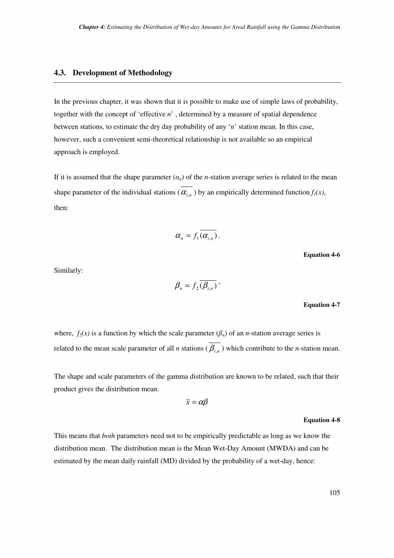
4.3.3. Estimation of n-Station-Mean Scale Parameter (βn)

The function fitted to the empirical relationship between βn / ni ,β and n’ takes the form:

)1(1 bxay −−−=’

Equation 4-10

where, in this case, a=0.8 and b=0.98 (Figure 4-15). This decay function is used because it

passes through the point y=1 when x=1 (i.e. an n-station average equivalent to 1 independent

station has the same scale parameter as a single station), and then levels off as x (n’) approaches

infinity, the ‘true’ areal mean.

The scale parameter of the station average, βn, is therefore calculated by:

[ ])1()(, anab

nin −+′= −ββ

Equation 4-11

112

Figure 4-15: Ratio of n-station to mean single-station β vs effective n (n’) for randomly selected

clusters of n stations from the UK (Blue), Zimbabwean (Green) and Chinese (Red) station data sets,

fitted with a negative exponential function. Plot symbols indicate different seasons: ◊= MAM,

=JJA, ∆∆∆∆=SON, x=DJF.

The values of βn estimated using Equation 4-11 are compared with the actual βn values,

determined by fitting a gamma distribution to the mean of the n available stations, for the random

clusters of n stations (Figure 4-16). This indicates that this approach is very successful over a

wide range of βn values. 95% confidence limits are estimated simply by finding the vertical

offsets necessary to encompass all but the 2.5% most positive and negative errors between the

estimated and actual values of βn. The assumption that the same confidence intervals apply to all

estimates regardless of the magnitude of either n’ or βn might be challenged on the basis of the

results shown in Figure 4-16 as it appears that the accuracy of the estimates increases with


113

decreasing values of βn, The accuracy of the estimated βn / ni ,β might also vary with the

magnitude of n’ (Figure 4-15). However, in these cases, there is not sufficient frequency of

points at the larger values in either case to determine whether this is warranted, and more

complex approaches to estimation error may suggest a higher degree of accuracy than can really

be offered by the data. This simple estimate is therefore applied to all cases values. The upper

and lower confidence bounds determined using this approach are +0.74 and -0.64, respectively

(Figure 4-15). This generalised approach may, however, result in broader uncertainty bounds for

some cases than is necessary (e.g. in cases where βn or βN is less than 3).

Figure 4-16: Estimated βn compared with actual βn for randomly selected clusters of n stations from

the UK (Blue), China (Red) and Zimbabwe (Green), with 95% confidence intervals. Plot symbols

indicate different seasons: ◊= MAM, =JJA, ∆∆∆∆=SON, x=DJF.

114

4.3.4. Estimation of n-Station-Mean Shape Parameter (αn)

The estimates of βn are now used together with estimates of nMD and P(d)n to estimate the shape

parameter for the distribution of the n-station mean (αn).

[ ]nn

n

ndP

MD

)(1−=

βα

Equation 4-12

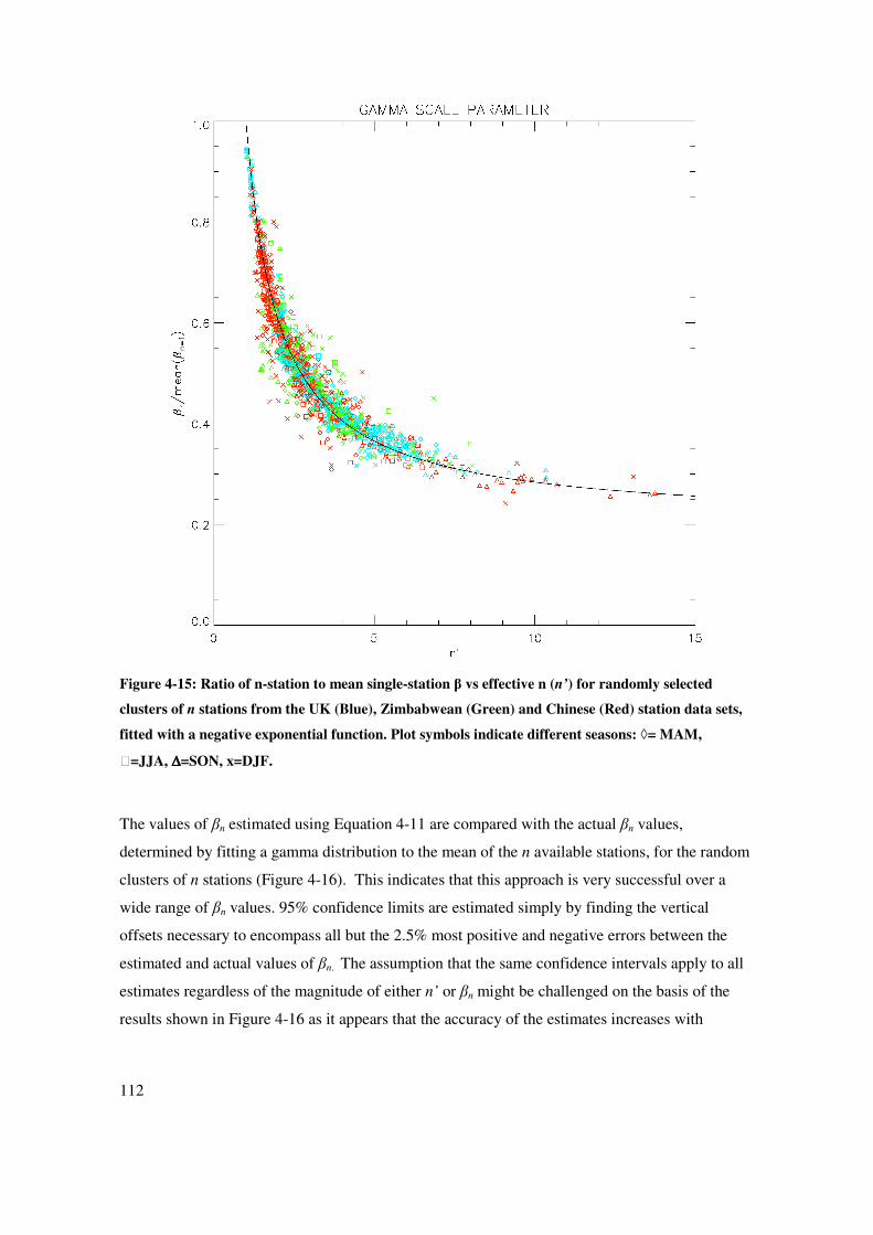
These estimates are compared to the actual values for the randomly selected clusters of n stations

in Figure 4-17. Although these estimates are relatively good (95% of the actual αn lie between

+0.28 and -0.11 of the estimated values), there are some systematic differences in skill between

regions. The different regions are shown separately in Figure 4-18, and demonstrate that while

this approach is very effective for the UK, as the estimates of αn consistently lie within close

range of the actual values across the range of different αn values, it is less successful for

Zimbabwe, for which the αn estimates deviate from the actual αn in a more systematic way,

overestimating at the top end of the range of values, and underestimating at the lower end of the

range. In the case of China, there is not a systematic bias in the slope of the relationship, but

there is a wide scatter, particularly towards underestimation of the shape parameters. The goal

that the method developed for estimating properties of an areal mean should be universally

applicable so that it can be transferred to other regions than those on which it is developed, means

that it is important to investigate the reasons behind these regional differences.


115

Figure 4-17: Estimated αn compared with actual αn for randomly selected clusters of n stations from

the UK (Blue), China (Red) and Zimbabwe (Green). Plot symbols indicate different seasons: ◊=

MAM, =JJA, ∆∆∆∆=SON, x=DJF.

116


the UK (Blue), Zimbabwe (Green) and China (Red). Plot symbols indicate different seasons: ◊=

MAM, =JJA, ∆∆∆∆=SON, x=DJF.

The error associated with the estimation of αn may be related to two possible sources:

a) Error is introduced via the estimated parameters P(d)n and βn which are used to estimate

αn. The errors associated with both these parameters have already been explored, for

P(d)n in Chapter 3 (Section 3.4.2), and for βn in Section 4.3.3. These errors are known

not to occur systematically for the different regions, and therefore it is unlikely that

these errors alone cause the errors in αn.


117

b) Error may also be introduced if the relationship αβ=x is a poor representation of the

data. This could occur for one of two reasons.

o The MWDA amount (the distribution mean) is calculated by the mean daily

rainfall ( NMD ) divided by the wet day probability (1-P(d)N) which is the

equivalent of dividing the total rainfall over all days by the number of wet-days.

A discrepancy may occur between a MWDA that is calculated in this way rather

than as the mean over all ‘wet’ days (>0.3mm) if the total of non-‘wet-day’

amounts (those between 0 and 0.3 mm) makes up a significant proportion of total

rainfall. This is likely to affect particularly dry regions and/or seasons, and may

therefore explain lack of skill for those particular cases.

o If the gamma distribution is not a perfect fit to the n-station series, the ‘actual’

shape and scale parameters may be inaccurate and their product may not equal

the mean of the sample. This is a possible outcome because the maximum

likelihood method that is used to fit the distribution finds the best parameters for

the observations, but does not necessarily choose parameters whose product

equals the sample mean, as the method of moments would. This is likely to

become a problem in regions with a small sample of data or where the gamma

distribution is a poorer fit to the data. These limitations may particularly apply to

drier regions/seasons where there are fewer ‘wet days’ to which the distribution

is fitted (i.e. a smaller sample of data).

The proportion of the error which can be attributed to these two sources is explored by calculating

αn from Equation 4-8 using the actual P(d)n and βn values that are determined by fitting gamma

distributions to the n-station mean series for each sample. This removes error caused by the

estimation of these parameters, leaving the error caused by the assumption that αnβn=MWDA.

Figure 4-19 therefore shows a comparison between the actual αn values (determined by fitting the

gamma distribution to the n-station mean) and the αn values estimated using Equation 4-12 and

the actual values of P(d)n and βn. . It is evident that for the Chinese dataset, almost exclusively for

winter, there is substantial error in estimated αn even when it is calculated from known values of

118

the P(d) and βn. This error is largest for larger values of αn, reaching +2 or more in the worst

cases. These poorly estimated values for the Chinese winter are distinct from the other regions

and seasons, for which the estimates are all very good and deviate only fractionally from the

actual values.


the UK (Blue), Zimbabwe (Green) and China (Red), when estimated αn values are based on actual βn

and P(d)n. Plot symbols indicate different seasons: ◊= MAM, =JJA, ∆∆∆∆=SON, x=DJF.


119

The substantial error that affects the Chinese winter values must therefore originate either

because for the fitted gamma parameters, αβ≠x (this may arise due to small sample size and/or

the gamma distribution fitting the data poorly), or because the exclusion of values <0.3 mm

causes errors in the estimation of MWDA. Plotting the size of the error against the mean daily

rainfall for each set of stations used demonstrates that it is the driest cases where this error is the

largest (Figure 4-20), with the large deviations affecting points where mean daily rainfall is less

than 0.3mm. However, these errors do not affect all the dry regions/seasons, as the Zimbabwean

dry season, JJA, has many points where mean daily rainfall is less than 0.3mm which do not

suffer from the same problems as the Chinese data.

Figure 4-20: Error in estimates of αn when based on actual values of βn and P(d)n compared with

mean daily rainfall (mm) for randomly selected clusters of n stations from the UK (Blue), Zimbabwe

(Green) and China (Red). Plot symbols indicate different seasons: ◊= MAM, =JJA, ∆∆∆∆=SON, x=DJF.

120

If the cases where mean daily rainfall is less than 0.3mm are excluded and Figure 4-17 is re-

plotted, an impression of the level of accuracy afforded by this estimation approach which is

appropriate to all remaining station cluster combinations is indicated using 95% confidence

intervals (Figure 4-21). These confidence intervals are now +0.18 and -0.09, a sizeable

improvement to the +0.28 and -0.11 bounds which were based on all points.

Splitting this cluster of points into different regions again (Figure 4-22) demonstrates that without

the cases where mean daily rainfall is less than 0.3mm, the performance is more consistent across

regions. The Zimbabwean data still demonstrates some overestimation for the higher values of

αn, and this overestimation appears to increase for larger values of αn. For the values of αn that are

within the range of the ‘example’ clusters of stations used here, the uncertainty bounds of +0.18

and -0.09 are reasonable enough to give useful estimates of the gamma parameters for grid-box

precipitation. However, these confidence bounds apply only to values of αn that lie within the

range covered by these station clustered of 0.5 to 1.5, and values beyond 1.5 may incur a larger

error margin.


121


the UK (Blue), China (Red) and Zimbabwe (Green), excluding cases where mean daily rainfall is less

than 0.3mm and with 95% confidence intervals +0.18 and -0.09. Plot symbols indicate different

seasons: ◊= MAM, =JJA, ∆∆∆∆=SON, x=DJF.

122


the UK (Blue), China (Red) and Zimbabwe (Green), excluding cases where mean daily rainfall is less

than 0.3mm. Plot symbols indicate different seasons: ◊= MAM, =JJA, ∆∆∆∆=SON, x=DJF.


123

4.3.5. Summary

The ratio of the gamma scale parameter of the distribution of wet-day rainfall amounts at

individual stations to that of an n-station average has been found to relate to the effective

independent sample size, n’, for a sample of n stations. This empirical relationship is used to

estimate the scale parameter of an n-station average series using the average scale parameter of

all n individual stations and the ‘effective n’ value for those stations, which is calculated via the

inter-station correlation between the wet days of the n stations.

When applied to example station clusters from the UK, China and Zimbabwe, the estimates of the

scale parameter for an n-station average are found to be reasonably accurate, with 95% of all

cases (based on 200 randomly selected clusters of n stations from each region, each of which has

points plotted separately for each season) lying within +0.74 and -0.64 mm of the actual values of

the scale parameter obtained when a distribution is fitted directly to the n-station average.

The scale parameter is used, together with the distribution mean (mean wet-day amount), to

estimate the shape parameter for the distribution of values in the same n-station average series’.

These estimates show larger error when compared to the actual distribution parameters in some

cases. Those cases where the error is the greatest tend to be those which experience the driest

climates, specifically the Chinese winter. These regions may experience large errors due to (a)

errors in fitting a distribution where there is less rainfall to model and/or (b) errors in calculating

the mean wet day amount using a rainfall total which includes the < 0.3mm values which are

excluded from the fitted distribution.

When very dry regions/seasons (where mean daily rainfall is less than 0.3mm) are excluded, the

estimates of the gamma shape parameter of an n-station mean series are found to be reasonably

good, with 95% of points lying within +0.18 and -0.09.

124

4.4. Application of Methodology to the Estimation of Gamma Parameters of ‘True’

Areal Mean Precipitation

It has been demonstrated in Section 4.3 that the distribution of wet day amounts in an n-station

mean can be estimated using an empirically derived relationship to predict the scale parameter,

from which the shape parameter can be derived via the mean wet day amount using the

relationship αβ=x This approach is now extended to the estimation of the gamma parameters

of a true areal mean, where the mean of an infinite number of stations, N, gives a grid-box mean.

This is illustrated using the same example UK grid box as was used in Chapter 3, containing 58

stations. The example grid box is then used to investigate the additional uncertainty introduced

by extrapolating to N from small values of n, and explore how this level of uncertainty varies with

the number of stations available (n) on which to base the estimates.

4.4.1. Extension of Methodology to the Estimation of Gamma Parameters of the

‘True’ Areal Mean

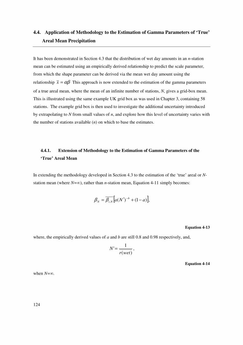
In extending the methodology developed in Section 4.3 to the estimation of the ‘true’ areal or N-

station mean (where N=∞), rather than n-station mean, Equation 4-11 simply becomes:

[ ])1()(, aNab

NiN −+′= −ββ ,

Equation 4-13

where, the empirically derived values of a and b are still 0.8 and 0.98 respectively, and,

)(

1'

wetrN = ,

Equation 4-14

when N=∞.


125

Equation 4-12 becomes:

[ ]])(1 NN

N

NdP

MD

−=

βα

Equation 4-15

It is necessary therefore to estimate the new values of :

(a) the average gamma scale parameter of station observations, Ni ,β ,

for the grid box, and the mean daily rainfall of station observations,

MDN , for the grid box, and;

(b) the average inter-station correlation of wet-day amounts, )(wetr , for

the grid box.

As was the case for the similar case of estimating P(d)N in Chapter 3 (Section 3.5), the estimation

of these values also incurs an additional uncertainty, which is also explored in the following

sections.

126

4.4.1.1. Estimating Mean Inter-Station Wet-Day Correlation for N Stations

In 3.4.1.1, correlation decay curves were used to estimate the mean inter-station correlation for

the whole grid box, instead of using the mean correlation between available stations, to give an

estimate of mean inter-station correlation for a grid box that is not biased by the particular sample

of station locations available. This same method is used here for wet-day correlation. Decay

curves are fitted for each station to its correlation with every other station in the UK dataset.

Some example correlation decay curves are shown in Figure 4-23.

In the majority of cases, the exponential function bdaewetr −=)( gives a good fit, at least for d

(separation distance) values up to around 400km, but for some stations, such as Cardington in

Figure 4-23 there is more scatter and therefore a wider range of possible positions or shapes for

the curve. For stations such as Stansted or Cardington, particularly in summer, the correlations

become negative for large separation distances and the exponential function does not fit well for

large d values, but this is acceptable as long as the curve fit is good up to the maximum separation

distance possible within the grid box (~400km). The curves fitted for r(wet) do not have such a

large ‘nugget’ as the curves fitted to r(wet/dry) shown in Section 3.4.1(i), passing much closer to

r(wet)=1 when d=0.


127

Figure 4-23: Example Correlation decay curves from four stations (Batheaston, Cardington, Oxford

and Stansted) from within the example UK grid box for JJA (left) and DJF (right).

128

The station correlation decay curves are then used to estimate a correlation decay curve for the

grid box by averaging the parameters of the curves from each of the n stations available, shown in

Figure 4-24. An r(wet) value for each of the 5000 randomly selected separation distances is then

estimated from this grid-box curve, and these are then averaged to obtain a mean inter-station

correlation value.

Figure 4-24: Grid-box average correlation decay curve (red) with those for each individual station

(black).

The grid-box )(wetr values, estimated using the curves in Figure 4-24 for the UK example grid

box, are given in Table 4-1 along with their corresponding N’ values for N=∞. These again show

notably lower correlation values for Summer (JJA) than for the other seasons, and therefore a

higher value of N’. The )(wetr values that have been calculated directly from the n available

stations are a little lower than those values for N stations, for all seasons except SON. This


129

suggests that the mean of the 58 available stations is less representative of the wet-day values true

of the areal mean than it is for the wet-day occurrences (see the similar comparison for the r(w/d)

values in the previous chapter, Section Table 3-2). This indicates that a greater density of station

coverage is required to give the distribution of wet-day amounts than to give the number of wet-

days in an average of individual stations which is intended to represent the true areal mean.

MAM JJA SON DJF

r(wet) for N stations

(mean r(wet) from available n stations)

0.45

(0.37)

0.37

(0.31)

0.49

(0.52)

0.55

(0.50)

N’

(n’)

2.22

(2.70)

2.70

(3.23)

2.04

(1.92)

1.82

(2.00)

Table 4-1: ‘True’ grid box mean r(wet) and N′ for an example UK grid box. The same values are

calculated, given in brackets, directly from the n available (58) stations for comparison.

4.4.1.2. Estimating Mean Station Gamma Scale Parameter and Mean Daily

Rainfall for N Stations

The value of Ni ,β is estimated using the arithmetic mean of β at the available stations ( ni ,β , thus

assuming that these available stations are representative of the grid box. The same principle is

applied for MDN. As has been discussed for the dry-day probability in Section 3.4.1.2, the degree

to which this assumption is valid will depend on the characteristics of a particular grid box and

the station coverage of available stations in that box. As the stations in this example grid box are

densely and evenly distributed within the grid box, and the region is relatively homogeneous in

topography and therefore in rainfall regime, the mean of the 58 station β values is assumed to

give a reasonable approximation to Ni ,β , and likewise MDn is considered representative of MDN.

130

4.4.2. Estimated Gamma Parameters for ‘True’ Areal Mean

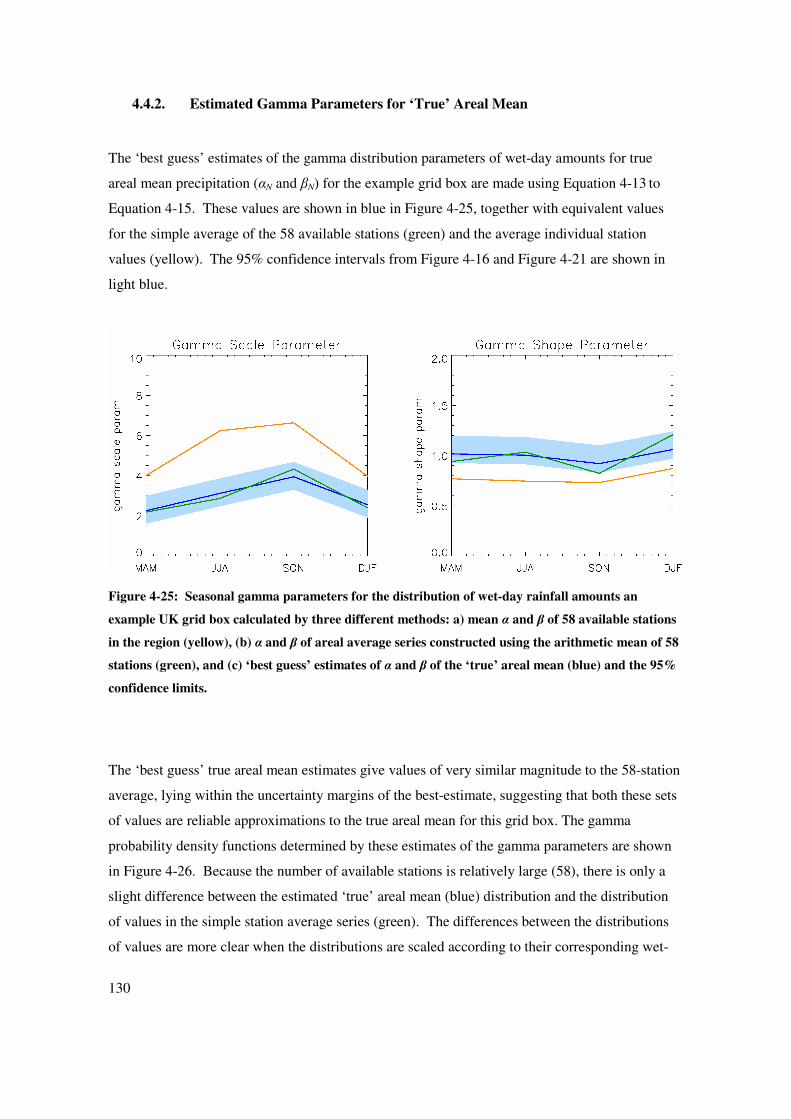
The ‘best guess’ estimates of the gamma distribution parameters of wet-day amounts for true

areal mean precipitation (αN and βN) for the example grid box are made using Equation 4-13 to

Equation 4-15. These values are shown in blue in Figure 4-25, together with equivalent values

for the simple average of the 58 available stations (green) and the average individual station

values (yellow). The 95% confidence intervals from Figure 4-16 and Figure 4-21 are shown in

light blue.

Figure 4-25: Seasonal gamma parameters for the distribution of wet-day rainfall amounts an

example UK grid box calculated by three different methods: a) mean α and β of 58 available stations

in the region (yellow), (b) α and β of areal average series constructed using the arithmetic mean of 58

stations (green), and (c) ‘best guess’ estimates of α and β of the ‘true’ areal mean (blue) and the 95%

confidence limits.

The ‘best guess’ true areal mean estimates give values of very similar magnitude to the 58-station

average, lying within the uncertainty margins of the best-estimate, suggesting that both these sets

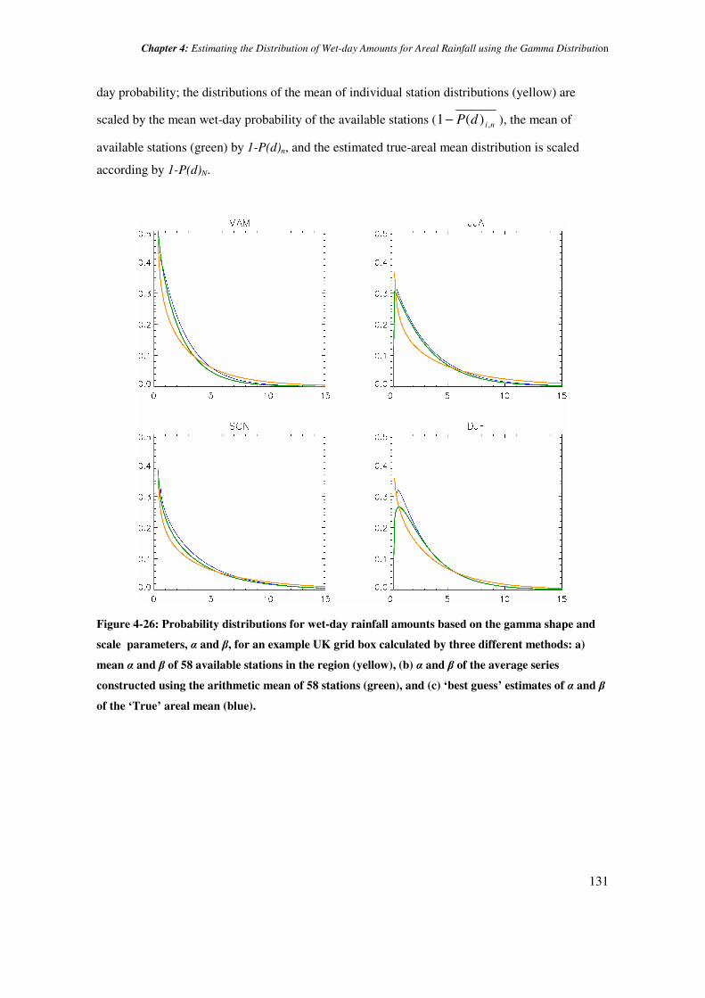
of values are reliable approximations to the true areal mean for this grid box. The gamma

probability density functions determined by these estimates of the gamma parameters are shown

in Figure 4-26. Because the number of available stations is relatively large (58), there is only a

slight difference between the estimated ‘true’ areal mean (blue) distribution and the distribution

of values in the simple station average series (green). The differences between the distributions

of values are more clear when the distributions are scaled according to their corresponding wet-


131

day probability; the distributions of the mean of individual station distributions (yellow) are

scaled by the mean wet-day probability of the available stations ( nidP ,)(1− ), the mean of

available stations (green) by 1-P(d)n, and the estimated true-areal mean distribution is scaled

according by 1-P(d)N.

Figure 4-26: Probability distributions for wet-day rainfall amounts based on the gamma shape and

scale parameters, α and β, for an example UK grid box calculated by three different methods: a)

mean α and β of 58 available stations in the region (yellow), (b) α and β of the average series

constructed using the arithmetic mean of 58 stations (green), and (c) ‘best guess’ estimates of α and β

of the ‘True’ areal mean (blue).

132

Figure 4-27: As for Figure 4-26 but the distributions are scaled according to their corresponding wet-

day probability.


133

4.4.3. Additional Uncertainty in Estimates of αN and βN for Small Values of n

In extending the methodology to allow for the extrapolation to large values of N, an additional

level of uncertainty is introduced when the values of )(wetr and Ni ,β for the grid box are

estimated from the n available stations. The example grid box given has a dense station coverage

at n=58, such that these estimates are likely to be relatively reliable. However, for cases where n

is considerably smaller than 58, and the methodology developed in this study is therefore

potentially more necessary, the estimated values required by the method become less certain as

they are based on information from fewer data points. In this section, sub-samples of n stations

from the available 58 in the example grid box are used to investigate the range of values, and

hence the additional uncertainty encountered, when smaller numbers of stations are available.

The method used is similar to that used for the dry-day probability in 3.4.1.1. Up to 30

combinations of n-stations are selected randomly, for values of n from 3 to 50. The results from

this investigation are shown in Figures 5-20 to 5-22. The range of values of the gamma scale and

shape parameters around the ‘best guess’ when all 58 stations are used are approximated for n

values up to 10, and 10 to 30, indicated by the shaded regions, and are intended simply as an

indication of the further uncertainties that might affect estimates, rather than as an accurate

quantification of uncertainty.

The range of values for the gamma scale parameter are approximated at +/-0.6 for values of n less

than 10 (Figure 4-28). This additional uncertainty is approximately halved for sample sizes 10 to

30 to +/-0.3. For the gamma shape parameter, these values are +/- 0.12 for n<10 and +/-0.06 for

10<n<30 (Figure 4-29).

134

Figure 4-28: Variations in estimated gamma scale parameter, β, of the ‘true’ areal mean rainfall

when, based on random sub-samples of n stations out of the available 58.

Figure 4-29: Variations in estimated gamma scale parameter, β, of the ‘true’ areal mean rainfall

when, based on random sub-samples of n stations out of the available 58.


135

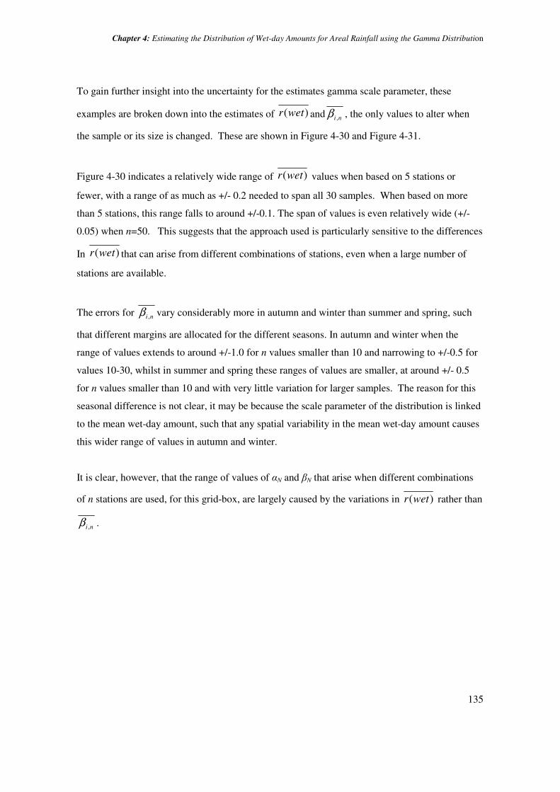
To gain further insight into the uncertainty for the estimates gamma scale parameter, these

examples are broken down into the estimates of )(wetr and ni ,β , the only values to alter when

the sample or its size is changed. These are shown in Figure 4-30 and Figure 4-31.

Figure 4-30 indicates a relatively wide range of )(wetr values when based on 5 stations or

fewer, with a range of as much as +/- 0.2 needed to span all 30 samples. When based on more

than 5 stations, this range falls to around +/-0.1. The span of values is even relatively wide (+/-

0.05) when n=50. This suggests that the approach used is particularly sensitive to the differences

In )(wetr that can arise from different combinations of stations, even when a large number of

stations are available.

The errors for ni ,β vary considerably more in autumn and winter than summer and spring, such

that different margins are allocated for the different seasons. In autumn and winter when the

range of values extends to around +/-1.0 for n values smaller than 10 and narrowing to +/-0.5 for

values 10-30, whilst in summer and spring these ranges of values are smaller, at around +/- 0.5

for n values smaller than 10 and with very little variation for larger samples. The reason for this

seasonal difference is not clear, it may be because the scale parameter of the distribution is linked

to the mean wet-day amount, such that any spatial variability in the mean wet-day amount causes

this wider range of values in autumn and winter.

It is clear, however, that the range of values of αN and βN that arise when different combinations

of n stations are used, for this grid-box, are largely caused by the variations in )(wetr rather than

ni ,β .

136

Figure 4-30: Variations in estimated grid-box mean inter-station wet-day correlation of rainfall,

)(wetr , based on random sub-samples of n stations out of the available 58.

Figure 4-31: Variations in estimated grid-box mean single-station gamma scale parameter,1=nβ ,

based on random sub-samples of n stations out of the available 58.


137

4.5. Estimating Distribution Extremes Using the Gamma Parameters

Having established that it is possible to estimate the distribution parameters for n-station or areal

rainfall averages, these parameters may also be useful for estimating the extremes of the

distribution, which are often of particular interest to the users of climate models due to their

severe impacts.

The gamma distribution has been used to study ‘extremes’ of daily rainfall in several studies

including (Groisman et al., 1999; Watterson and Dix, 2003; May, 2004). The term ‘extreme’ can

be interpreted in several different ways. Many studies of extremes use annual maximum values

only and fit an extreme value distribution such as the Gumbel distribution or the Generalised

Extreme Value distribution (GEV) to these values. These can then be used to estimate extreme

rainfall values for return periods of, say, 20, 50 or 100-years. The ‘extremes’ referred to here,

however, are the 90th, 95

th and 99

th percentile values (P90, P95 and P99 from hereon) of the

gamma distribution, which represent events that occur, approximately, once in every 10, 20 or

100 wet days (when their frequency is averaged over long periods of time). Whilst these values

are less ‘extreme’ than those used in many other extreme value studies the percentile values used

here are widely used in climate impacts work because they require less data to model accurately

and provide useful information for the users of climate model data and climate impact studies.

The following section will investigate how reliably the percentile values are estimated for areal

rainfall when derived from the estimated parameters of the gamma distribution.

4.5.1. Assessment of Goodness-of-Fit at Distribution Tails

Before using the estimated gamma parameters to estimate percentile values, it is important to

assess how well the gamma distribution fits the data at the tails. It is to be expected that the

higher extremes will be less well modeled by the fitted distribution, as there are fewer values on

which to fit the model (Koning and Franses, 2005). We therefore look for the highest percentile

value that can be estimated reliably. The Q-Q plots shown in Figure 4-4 to Figure 4-9 in 4.2.3

demonstrated that for the examples studied, the fitted distributions give a good fit up to the 95th

percentile, above which the distribution tends to underestimate the wet-day rainfall values. The

138

use of the P99 is therefore unlikely to be able to provide a reliable estimate, but the P90 and P95

are expected to be more reliably estimated.

This is assessed for a larger number of examples by plotting the fitted percentile value versus the

actual value for examples from all three study regions (Figure 4-32). In order to avoid the worst

fitting cases, those where the number of available data points with which to fit the distribution is

less than 100, are excluded. Figure 4-32 confirms that a substantial deterioration in fit occurs at

P99, but that the fit is relatively good up to P95. From here on, only P95 will be used as this is the

highest extreme value that can be modeled reliably.

Figure 4-32: Percentile threshold values from the fitted distribution compared with those calculated

directly from data for 90th

, 95th

and 99th

percentiles, for n-station average series’ from UK (blue),

China (red), and Zimbabwe (green).


139

4.5.2. Estimating Percentile Values from the Gamma Distribution

In order to test the estimates of P95 for the n-station average series (P95n) that are calculated via

the estimates of areal rainfall gamma distribution parameters (αn and βn), the estimates of P95 are

plotted against the ‘observed’ percentile values for the same n-station averages, made up from

randomly selected clusters of n stations from all 3 study regions. The ‘observed values’ can be

defined either as the percentile values calculated directly from the n-station average wet-day data,

or as the percentile values derived from the distribution fitted to the n-station average wet-day

data. These are both shown in Figure 4-33.

Figure 4-33: Estimated vs Observed values of P95n, when the Observed value is determined by (a)

the fitted distribution and (b) directly from the data.

The left hand plot in Figure 4-33 represents the error incurred by deriving P95n from the

estimated parameters αn and βn, and thus deviation in the estimated values form those that are

observed is caused by the errors in estimating αn and βn using the empirical approach developed in

Sections 4.3.3 and 4.3.4. The error margin is relatively narrow because the position of the tail and

extreme values of the distribution are largely dependent on the scale parameter, which is

estimated with narrow error margins in Section 4.3.3 (see Figure 4-16). The value of the shape

parameter, which has larger estimation errors, has less effect of the extreme percentiles.

140

The right hand plot shows a similar plot using the observed percentiles directly from the data, and

thus includes the error between the fitted distribution at P95n and the actual data value at P95n.

The distribution fit has been demonstrated to be good at P95 (4.5.1), and so this does not add

substantially to the overall estimation error.

From here on, the error estimation for P95n is defined by the latter of these ‘observed’ values (the

difference between the estimated P95n the value of P95n which is observed directly from the

data), so that the distribution-fit error is incorporated. It might be expected that this error in the

distribution fit will vary depending on the number of wet day data values available for fitting the

distribution to (nwet). If the fit error is demonstrated to relate to nwet, then the overall error could

be estimated more explicitly by using a fitted relationship between these two values. This is

tested by plotting the error against nwet for each case and shown in Figure 4-34. Whilst the

largest errors tend to occur where nwet is low, many examples of low nwet fit well resulting in a

low error, and therefore there is not a strong relationship between the two.

Figure 4-34: Relationship between the estimation error of P95n and the number of values on which

the distribution is fitted (nwet).

The estimates of error are therefore derived using confidence limits, which are fitted to

encompass 95% of the points in Figure 4-35. These values are estimated to be 3.17 and 0.36

above and below the estimated value, respectively. It should be noted that the error margins


141

estimated here are only appropriate when applied to cases where nwet is greater than 100, and

errors may be larger when a distribution is fitted to a smaller sample size.

Figure 4-35: 95% confidence limits for estimation of P95n.

142

4.6. Discussion and Summary

An empirical approach has been used in this study to relate the gamma distribution parameters of

wet day amounts in a grid-box areal mean to those at points within the grid box via the value of

the number of effective independent stations, n', which incorporates a measure of the spatial

dependence in that region. These estimates of the parameters of the gamma distribution or areal

rainfall can also be used to estimate the extreme values of the distribution using the 95th percentile

value of wet-day amounts. The resulting ‘best guess’ estimates of the ‘true’ areal mean for a grid

box are useful for quantitative assessment of GCM or RCM daily rainfall, which simulate grid-

box average quantities, and for other applications which require knowledge of areal precipitation

characteristics.

However, the degree to which these estimates can be considered as ‘useful’ in such applications

in dependent on the degree to which they can be relied upon. A range of uncertainty is suggested

for these estimates of αN and βN. The estimates of βN are found to be very good when based on a

large number of stations from within a grid box, within a range of +0.74 and -0.64. However,

investigation of the additional error that might be incurred when the estimates are based on

smaller numbers of stations suggest that this range might become twice as large, with an

additional +/-0.6 uncertainty when based on 10 stations or fewer, and an additional +/-0.3 for 10

to 30 stations.

The estimates of αN when calculated from the estimated values of βN and P(d)N, show greater

proportional error, with 95% of estimated values falling within +0.18 and -0.09 of the actual

values. This error is largely a result of the error estimation in the values P(d)N and βN, with which

αN is estimated. However, some additional error can be introduced to the estimates of αN in some

cases where mean daily rainfall is less than 0.3mm. This partly due to the fact that there are

insufficient wet-days in these very dry regions/seasons to allow a good fit to the gamma

distribution. The techniques developed for the estimation of the gamma distribution parameters

of areal rainfall are therefore recommended to be applied with caution for such dry

regions/seasons. This limitation to the approach for regions that are very dry may prove to

particularly disadvantageous as these which are least populated, and thus least well gauged.


143

In generalizing the uncertainty range for all regions and seasons upon which the methodology is

developed, the range inevitably becomes broader for some regions than might have been the case

if the uncertainty envelope were tailored to each particular region. This means that the

uncertainty bounds estimated here give an indication of the accuracy of the estimated ‘true’ areal

mean values, but that for specific regions or seasons, they maybe smaller.

The empirical relationship on βn is estimated from n' (Equation 4-11), and the 95% confidence

intervals which are estimated for those values (Figure 4-16), are established using data from three

regions. While the four seasons of the three regions represent a wide range of different climatic

conditions, they do not cover all possible climatic regimes. The regions used do not, for example,

include a region of very high elevation, which may experience differences in its climate due to its

topography. It may therefore be necessary to test the relationships before applying them to

regions with climatic regimes that differ considerably from all of the regions on which they are

based.

As these estimates are based on an empirical analysis, it is important to recognize that

extrapolation beyond the data on which the functions and uncertainty bounds are developed is

unwise. Specifically, the fitted function upon which the estimates are based in Figure 4-15 is

fitted to cases where n' is less than 14. It is unlikely that, at GCM grid scale, values of N' much

larger than this will arise often, as in order for a value of N' greater than 14 to arise based on

N=∞, )(wetr must be less than 0.07, which is unlikely even in regions where spatial dependence

is particularly low. If this technique is used in applications that require areal precipitation

estimates at a larger spatial scale then this may first require some further investigation to ensure

that the empirical relationships remain valid.

The uncertainties which accompany these estimates do not, however, de-value the estimates of

areal rainfall characteristics that have been developed here. Whilst the cases where the number or

distribution of stations is poorest are those which incur the greatest uncertainties, these are the

cases where the application of this technique yields the greatest benefit. The techniques should

be applied with due attention to the associated uncertainties.

144

4. Estimating the Distribution of Wet-Day Amounts for … 4 4. Estimating the Distribution of Wet-Day Amounts for Areal Rainfall Using the Gamma Distribution Contents 4.1. Introduction

Documents