4 Economic Costs (Students)

4 Economic Costs

Production Costs

Total production cost =(i.e. the cost of foregoing the opportunity to produce alternative goods & services).

Total production costs =

Explicit costs

The monetary payments to outside suppliers for supplying factors of production.

E.g. wages & salaries paid for labor services, cost of raw materials, payments for transport services, etc.

Implicit costs

The cost of using resources owned within the firm. Usually no outright payments are made.

E.g. depreciation (loss in value of buildings & machinery), entrepreneur’s risk-taking & time, normal profit.

Normal profit

The minimum profit that a firm must earn to stay in the current production.

Note: Normal profit is included in implicit costs.

Economic profit

Also known as Pure or Abnormal or Supernormal Profit

Economic Profit ==

(where TR = Price x Quantity sold)

Accounting profit

Accounting Profit =

Accounting profit > Economic Profit

Exercise:

Franco’s Pizza produces 100 pizzas a day.Price per pizza = $15Costs of tomatoes & pizza ingredients = $550Cost of electricity & water = $75Depreciation of oven = $50Wages = $250Minimum profit = $200

Q. Calculate Franco’s Pizza’s (i) economic profit, and (ii) accounting profit for a day.

Exercise:

The Short-Run

• That time period where certain factors of production can easily be varied to alter production, while some factors cannot.

E.g. To increase production, more labour can be hired, more raw materials can be bought, but cannot build another factory.

• Those factors of production that can easily be changed in quantity to alter output are called ________________.

E.g. labour, raw materials, electricity, water.• Factors of production that cannot be varied to alter output

are called _____________. E.g. heavy machinery, factories, land.

The Long-Run

• That time period long enough for all factors of production to be varied to alter output.

E.g. More labour can be hired, more factories can be built, more machinery can be installed.

• Therefore, in the long-run, there are __________________, only variable factors.

Note:Different firms in different markets may not have similar short-run or long-run time periods. The actual time period may be different for different firms.As long as there is at least _______ fixed factor, the firm is operating in the short-run.

Short-run production

We will look at what happens to output in the S/R when more or less of the variable factor are applied to a given fixed factor.

Assumptions:• Only 2 factors of production are used, i.e. labor (L) &

capital (K).• In the S/R, L is the variable factor, K is the fixed factor.

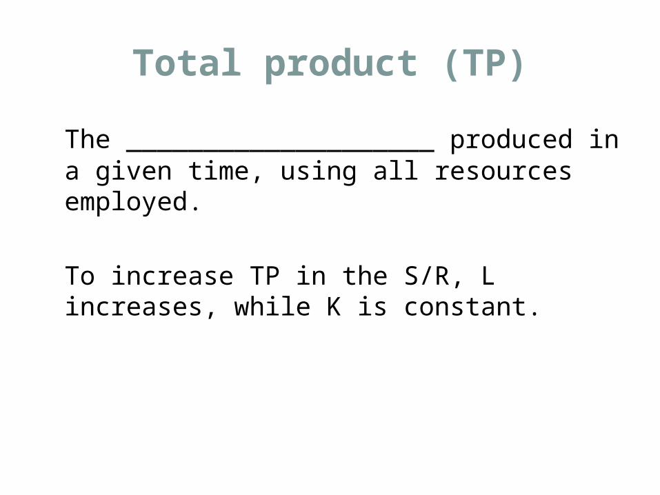
Total product (TP)

The ____________________ produced in a given time, using all resources employed.

To increase TP in the S/R, L increases, while K is constant.

Average product (AP)

The total product per unit of the variable factor. (e.g. output per worker)

AP = (where L is the quantity of labour)

Marginal product (MP)

The change in TP resulting from a one-unit change in the variable factor. (e.g. the additional output produced by an extra worker)

MP = (where is ‘change in’)

When MP falls, the firm is experiencing diminishing marginal returns/productivity.

Example:

Assume that K is fixed at 2 units.

Qty of Qty of LL

TPTP APAP MPMP

00 00 -- --

11 1515

22 3434

33 1616

44 1515

55 22

TP, AP, MP

Qty of labour (L)

The law of diminishing returns

• states that if increasing quantities of a variable factor are applied to a given fixed factor, there will come a point when an extra unit of the variable factor adds less to TP than the variable factor before it. (i.e. MP of the variable factor falls)e.g. as additional workers are hired to work on a fixed number of machines, there will come a time when an extra worker produces less than the previous worker.

Short-run production costs

We will look at how costs change as more or less of the variable factor are added to a given fixed factor to alter output.

Total fixed cost (TFC)

(also called overhead or unavoidable cost)• Cost of using the fixed factors.

E.g. rental, depreciation on buildings & machinery, insurance.

• TFC is __________, i.e. it does not change as output changes.

• Even if output is zero, TFC still has to be paid.

Total variable cost (TVC)

• Cost of using the variable factors. E.g. wages & salaries, payments for raw materials and electricity.

• TVC __________ as output increases (as more variable factors are hired).

• If output is zero; TVC is ______.

Total cost (TC)

• Cost of producing a certain level of output.

TC =

If output is zero; TC = _____.

Total costs for a firm

TC, TFC, TVC

Qty of output (Q)

Average fixed cost (AFC)

• Fixed cost per unit of output.

AFC = (where Q is quantity of output)

• As output (Q) increases; AFC _____ (i.e. spreading the overheads).

Average variable cost (AVC)

• Variable cost per unit of output.

AVC =

Average total cost (ATC or AC)

• Total cost per unit of output.

AC =

Marginal cost (MC)

• The change in TC resulting from a one-unit change in output. (The additional cost of producing one more unit of output.)

MC =

• When MP falls; MC _________ (diminishing returns).

Average and marginal costs

Cost per unit

Qty of output (Q)

Long-run production costs

• In the L/R, there are no fixed factors, therefore no fixed cost, only variable cost.

(Only look at AC, i.e. LRAC, and LRMC).

OutputO

Co

sts

A typical U-shaped long-run average cost curveA typical U-shaped long-run average cost curve

A typical bowl-shaped long-run average cost curve

OutputO

Co

sts

Economies of scale

• Where increasing the scale of production leads to ___________________ (falling LRAC).

Types of economies:• ____________ economies (e.g. larger machinery)• ____________ economies (e.g. lower bank interest rate)• ____________ economies (e.g. advertising & promotions)• ____________ economies (e.g. division of labour)• ____________ economies (e.g. product diversification)

Diseconomies of scale

• Where LRAC _________ as output expands.

Causes:• Problems of coordination & communication.• Increased monotony falling productivity.• Disruptions in long production lines.

Long-run average cost curve

OutputO

Co

sts

LRACEconomiesof scale

Constantcosts

Diseconomiesof scale

Revenue

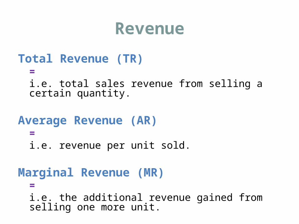
Total Revenue (TR)= i.e. total sales revenue from selling a certain quantity.

Average Revenue (AR)= i.e. revenue per unit sold.

Marginal Revenue (MR)= i.e. the additional revenue gained from selling one more unit.

Profit-maximising output level

Total economic profit = The profit-maximising firm will produce at that level of output where (TR-TC) is the greatest, i.e. where MC=MR.

2 approaches:Difference between TR-TC is the greatest.MC=MR.

Profit-maximising output level

1. Using total curves (TR-TC approach)

– maximising difference between TR and TC

-8

-6

-4

-2

0

2

4

6

8

10

12

14

16

18

20

22

24

1 2 3 4 5 6 7

TR

, TC

, T

(£

)

T

TR

TC

d

e

f

Quantity

Finding maximum profit using total curves

Profit-maximisingoutput

Profit-maximising output level

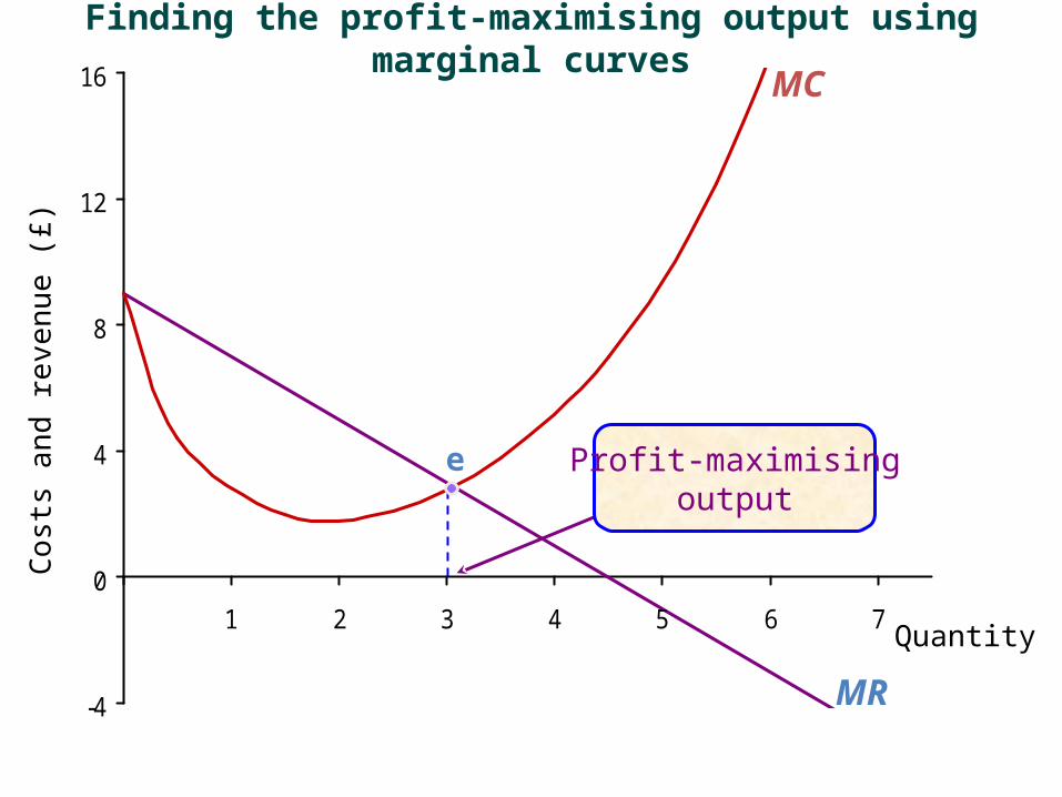
2. Using marginal and average curves (MR-MC approach)

– Profit is maximised where MR = MC.

Firms will produce output where MR>MC right up until MR=MC. Further production of output will leave MR<MC & losses will be made on those units above the MR=MC point.

-4

0

4

8

12

16

1 2 3 4 5 6 7Quantity

Co

sts

and

rev

enu

e (

£)

e

MR

MC

Profit-maximisingoutput

Finding the profit-maximising output using marginal curves