Ph.D. THESIS M. B. Patel 4 DATA COLLECTION & METHODOLOGY 55 DATA COLLECTION & METHODOLOGY 4 Data has been collected from Gujarat Water Resources Development Corporation Ltd. (GWRDC), Central Ground Water Board (CGWB), State Water Data Centre (SWDC), Vadodara Mahanagar Seva Sadan (VMSS), Central Water Commission (CWC), Water Resources Investigation Circle (WRIC), Vadodara Irrigation Circle (VIC), Mahi Irrigation Circle (MIC), Gujarat Engineering Research Institute (GERI), Sardar Sarovar Narmada Nigam Limited (SSNL) and Gujarat Electricity Corporation Ltd etc. are compiled and enlisted. The data to be used for model study as an input are prepared. In this chapter the model boundary is identified and construction of the model using GMS software is discussed. 4.1 RL’s of Mahi River Water Level Daily RL’s of Mahi water levels are collected at three sites namely Khanpur, Poicha and Dhuvaran for the duration June 1997 to June 1999, June 2003 to June 2005 and June 2005 to June 2007. RL’s at Khanpur are collected from the Central Water Commission (CWC), Gandhinagar, RL’s at Poicha are collected from Vadodara Mahanagar Seva Sadan (VMSS), Vadodara and RL’s at Dhuvaran are collected from Gujarat Electricity Corporation Ltd. This data is presented in Annexure-I and graphically plotted viz. graphs 4.1 to 4.6.

Welcome message from author
This document is posted to help you gain knowledge. Please leave a comment to let me know what you think about it! Share it to your friends and learn new things together.
Transcript
Ph.D. THESIS M. B. Patel
4 DATA COLLECTION & METHODOLOGY 55
DATA COLLECTION & METHODOLOGY 4
Data has been collected from Gujarat Water Resources Development Corporation Ltd.
(GWRDC), Central Ground Water Board (CGWB), State Water Data Centre (SWDC),
Vadodara Mahanagar Seva Sadan (VMSS), Central Water Commission (CWC), Water
Resources Investigation Circle (WRIC), Vadodara Irrigation Circle (VIC), Mahi Irrigation
Circle (MIC), Gujarat Engineering Research Institute (GERI), Sardar Sarovar Narmada
Nigam Limited (SSNL) and Gujarat Electricity Corporation Ltd etc. are compiled and
enlisted. The data to be used for model study as an input are prepared. In this chapter the
model boundary is identified and construction of the model using GMS software is discussed.
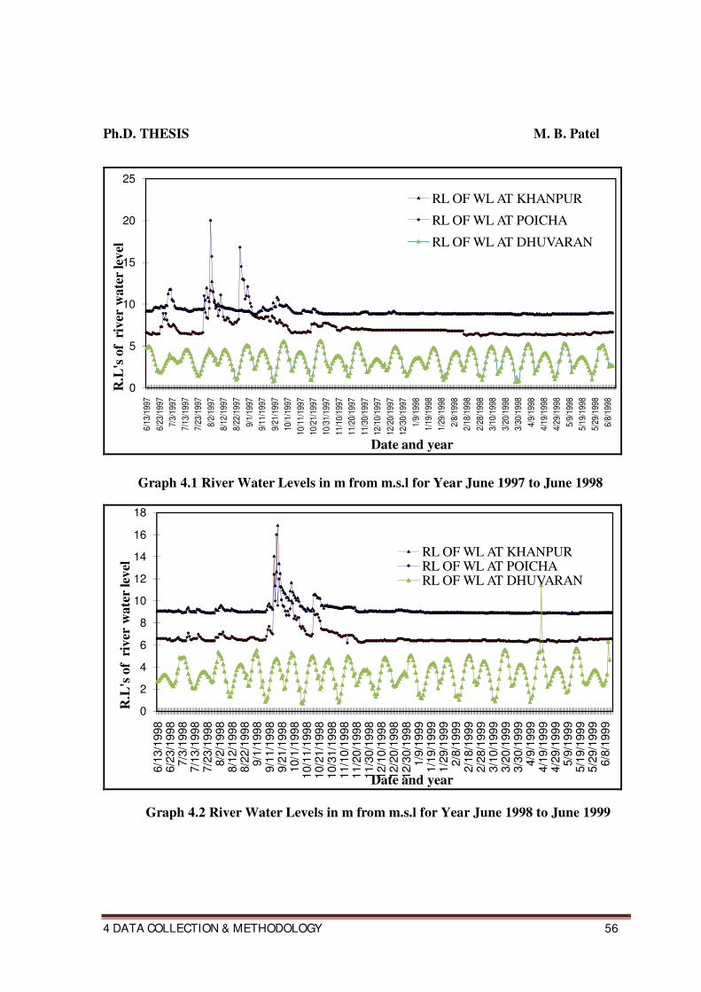
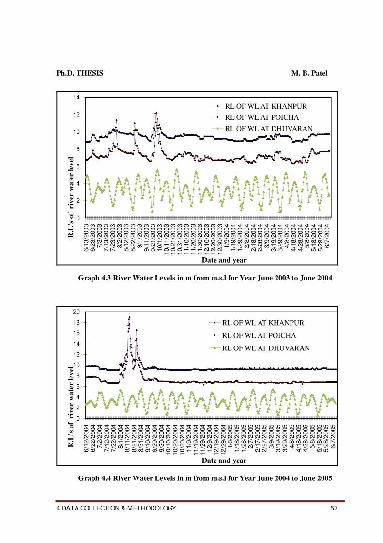
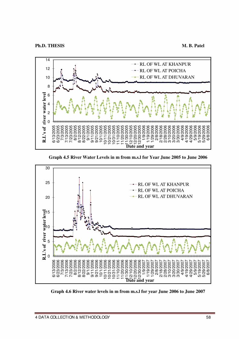
4.1 RL’s of Mahi River Water Level
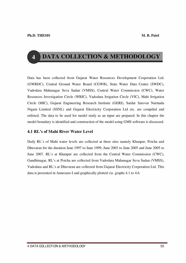
Daily RL’s of Mahi water levels are collected at three sites namely Khanpur, Poicha and
Dhuvaran for the duration June 1997 to June 1999, June 2003 to June 2005 and June 2005 to
June 2007. RL’s at Khanpur are collected from the Central Water Commission (CWC),
Gandhinagar, RL’s at Poicha are collected from Vadodara Mahanagar Seva Sadan (VMSS),
Vadodara and RL’s at Dhuvaran are collected from Gujarat Electricity Corporation Ltd. This
data is presented in Annexure-I and graphically plotted viz. graphs 4.1 to 4.6.
Ph.D. THESIS M. B. Patel
4 DATA COLLECTION & METHODOLOGY 56
Graph 4.1 River Water Levels in m from m.s.l for Year June 1997 to June 1998
Graph 4.2 River Water Levels in m from m.s.l for Year June 1998 to June 1999
0
5
10
15
20
25
6/1
3/1
997
6/2
3/1
997
7/3
/1997
7/1
3/1
997
7/2
3/1
997
8/2
/1997
8/1
2/1
997
8/2
2/1
997
9/1
/1997
9/1
1/1
997
9/2
1/1
997
10/1
/1997
10/1
1/1
997
10/2
1/1
997
10/3
1/1
997
11/1
0/1
997
11/2
0/1
997
11/3
0/1
997
12/1
0/1
997
12/2
0/1
997
12/3
0/1
997
1/9
/1998
1/1
9/1
998
1/2
9/1
998
2/8
/1998
2/1
8/1
998
2/2
8/1
998
3/1
0/1
998
3/2
0/1
998
3/3
0/1
998
4/9
/1998
4/1
9/1
998
4/2
9/1
998
5/9
/1998
5/1
9/1
998
5/2
9/1
998
6/8
/1998
R.L
's o
f r
iver
wate
r le
vel
Date and year
RL OF WL AT KHANPUR
RL OF WL AT POICHA
RL OF WL AT DHUVARAN
0
2
4
6
8
10
12
14
16
18
6/1
3/1
998
6/2
3/1
998
7/3
/1998
7/1
3/1
998
7/2
3/1
998
8/2
/1998
8/1
2/1
998
8/2
2/1
998
9/1
/1998
9/1
1/1
998
9/2
1/1
998
10/1
/1998
10/1
1/1
998
10/2
1/1
998
10/3
1/1
998
11/1
0/1
998
11/2
0/1
998
11/3
0/1
998
12/1
0/1
998
12/2
0/1
998
12/3
0/1
998
1/9
/1999
1/1
9/1
999
1/2
9/1
999
2/8
/1999
2/1
8/1
999
2/2
8/1
999
3/1
0/1
999
3/2
0/1
999
3/3
0/1
999
4/9
/1999
4/1
9/1
999
4/2
9/1
999
5/9
/1999
5/1
9/1
999
5/2
9/1
999
6/8
/1999
R.L
's o
f r
iver
wa
ter
level
Date and year
RL OF WL AT KHANPURRL OF WL AT POICHARL OF WL AT DHUVARAN
Ph.D. THESIS M. B. Patel
4 DATA COLLECTION & METHODOLOGY 57
Graph 4.3 River Water Levels in m from m.s.l for Year June 2003 to June 2004
Graph 4.4 River Water Levels in m from m.s.l for Year June 2004 to June 2005
0
2
4
6
8
10
12
14
6/1
3/2
003
6/2
3/2
003
7/3
/2003
7/1
3/2
003
7/2
3/2
003
8/2
/2003
8/1
2/2
003
8/2
2/2
003
9/1
/2003
9/1
1/2
003
9/2
1/2
003
10/1
/2003
10/1
1/2
003
10/2
1/2
003
10/3
1/2
003
11/1
0/2
003
11/2
0/2
003
11/3
0/2
003
12/1
0/2
003
12/2
0/2
003
12/3
0/2
003
1/9
/2004
1/1
9/2
004
1/2
9/2
004
2/8
/2004
2/1
8/2
004
2/2
8/2
004
3/9
/2004
3/1
9/2
004
3/2
9/2
004
4/8
/2004
4/1
8/2
004
4/2
8/2
004
5/8
/2004
5/1
8/2
004
5/2
8/2
004
6/7
/2004
R.L
's o
f r
iver
wa
ter
level
Date and year
RL OF WL AT KHANPUR
RL OF WL AT POICHA
RL OF WL AT DHUVARAN
0
2
4
6
8
10
12
14
16
18
20
6/1
2/2
004
6/2
2/2
004
7/2
/2004
7/1
2/2
004
7/2
2/2
004
8/1
/2004
8/1
1/2
004
8/2
1/2
004
8/3
1/2
004
9/1
0/2
004
9/2
0/2
004
9/3
0/2
004
10/1
0/2
004
10/2
0/2
004
10/3
0/2
004
11/9
/2004
11/1
9/2
004
11/2
9/2
004
12/9
/2004
12/1
9/2
004
12/2
9/2
004
1/8
/2005
1/1
8/2
005
1/2
8/2
005
2/7
/2005
2/1
7/2
005
2/2
7/2
005
3/9
/2005
3/1
9/2
005
3/2
9/2
005
4/8
/2005
4/1
8/2
005
4/2
8/2
005
5/8
/2005
5/1
8/2
005
5/2
8/2
005
6/7
/2005
R.L
's o
f r
iver
wate
r le
vel
Date and year
RL OF WL AT KHANPUR
RL OF WL AT POICHA
RL OF WL AT DHUVARAN
Ph.D. THESIS M. B. Patel
4 DATA COLLECTION & METHODOLOGY 58
Graph 4.5 River Water Levels in m from m.s.l for Year June 2005 to June 2006
Graph 4.6 River water levels in m from m.s.l for year June 2006 to June 2007
0
2
4
6
8
10
12
14
6/1
3/2
005
6/2
3/2
005
7/3
/2005
7/1
3/2
005
7/2
3/2
005
8/2
/2005
8/1
2/2
005
8/2
2/2
005
9/1
/2005
9/1
1/2
005
9/2
1/2
005
10/1
/2005
10/1
1/2
005
10/2
1/2
005
10/3
1/2
005
11/1
0/2
005
11/2
0/2
005
11/3
0/2
005
12/1
0/2
005
12/2
0/2
005
12/3
0/2
005
1/9
/2006
1/1
9/2
006
1/2
9/2
006
2/8
/2006
2/1
8/2
006
2/2
8/2
006
3/1
0/2
006
3/2
0/2
006
3/3
0/2
006
4/9
/2006
4/1
9/2
006
4/2
9/2
006
5/9
/2006
5/1
9/2
006
5/2
9/2
006
6/8
/2006
R.L
's o
f r
iver
wate
r le
vel
Date and year
RL OF WL AT KHANPUR
RL OF WL AT POICHA
RL OF WL AT DHUVARAN
0
5
10
15
20
25
30
6/1
3/2
006
6/2
3/2
006
7/3
/2006
7/1
3/2
006
7/2
3/2
006
8/2
/2006
8/1
2/2
006
8/2
2/2
006
9/1
/2006
9/1
1/2
006
9/2
1/2
006
10/1
/2006
10/1
1/2
006
10/2
1/2
006
10/3
1/2
006
11/1
0/2
006
11/2
0/2
006
11/3
0/2
006
12/1
0/2
006
12/2
0/2
006
12/3
0/2
006
1/9
/2007
1/1
9/2
007
1/2
9/2
007
2/8
/2007
2/1
8/2
007
2/2
8/2
007
3/1
0/2
007
3/2
0/2
007
3/3
0/2
007
4/9
/2007
4/1
9/2
007
4/2
9/2
007
5/9
/2007
5/1
9/2
007
5/2
9/2
007
6/8
/2007R
.L's
of
riv
er w
ate
r le
vel
Date and year
RL OF WL AT KHANPUR
RL OF WL AT POICHA
RL OF WL AT DHUVARAN
Ph.D. THESIS M. B. Patel
4 DATA COLLECTION & METHODOLOGY 59
4.2 RL’s of Ground Level of Wells and River Bed
Reduced levels of ground levels of wells, piezometers, villages, river banks, river bed etc are
collected from agencies like GWRDC, WRIC, VIC, CGWB and CWC. The river bed data
have been completed by interpolating intermediate values in software surfer. These data have
been contained in Annexure-II.
4.3 RL’s of Bottom of Wells in Unconfined Aquifer
Contours of bottom of unconfined aquifer in Sardar Sarovar Command area (Source:
Wallingford and Shah, (1994) “Data for Groundwater Model of Sardar Sarovar Command
Area” Sponsored by Narmada Planning Group, Gandhinagar. Vol. III- Plates) have been
transferred to base map of study area. They are used to work out RL’s of bottom of wells by
interpolation. They are presented in Annexure-III.
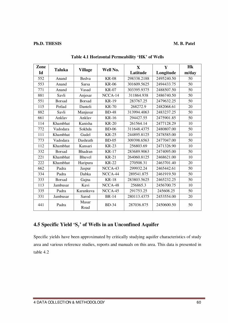
4.4 Horizontal Permeability ‘HK’ of Wells in an Unconfined Aquifer
Horizontal permeability of aquifer is estimated by superimposing figure of aquifer
permeability zones of Sardar Sarovar Command area given in EX3183: Main Report,
November 1995, Wallingford, by interpolation. They are represented in table 4.1
Ph.D. THESIS M. B. Patel
4 DATA COLLECTION & METHODOLOGY 60
Table 4.1 Horizontal Permeability ‘HK’ of Wells
Zone
Id Taluka Village Well No.
X
Latitude
Y
Longitude
Hk
m/day
552 Anand Bedva KR-08 298338.2188 2495240.50 50
553 Anand Sarsa KR-06 301609.5625 2494433.75 50
771 Anand Vasad KR-07 303395.9375 2488507.50 50
881 Savli Anjesar NCCA-14 311864.938 2486740.50 50
551 Borsad Borsad KR-19 283767.25 2479632.25 50
115 Petlad Danteli KR-70 268272.9 2482068.61 20
882 Savli Manjusar BD-48 313994.4063 2483237.25 50
661 Anklav Anklav KR-16 294427.55 2475901.85 50
114 Khambhat Kanisha KR-20 261564.14 2477128.29 10
772 Vadodara Sokhda BD-06 311648.4375 2480807.00 50
111 Khambhat Gudel KR-25 244895.8125 2478585.00 10
773 Vadodara Dashrath BD-05 309398.6563 2477047.00 50
112 Khambhat Kansari KR-23 256803.69 2471326.90 10
332 Borsad Bhadran KR-17 283689.9063 2474095.00 50
221 Khambhat Bhuvel KR-21 264060.8125 2468621.00 10
222 Khambhat Haripura KR-22 270508.31 2463701.40 20
662 Padra Jaspur NCCA-43 299932.24 2465442.61 50
334 Padra Dabka NCCA-44 289541.875 2461919.50 50
333 Borsad Gajna KR-18 283803.5625 2465232.25 50
113 Jambusar Kavi NCCA-48 256865.3 2456700.75 10
335 Padra Karankuva NCCA-45 291753.25 245608.25 50
331 Jambusar Sarod BR-14 280113.4375 2453554.00 20
441 Padra Masar
Road BD-34 287036.875 2450600.50 50
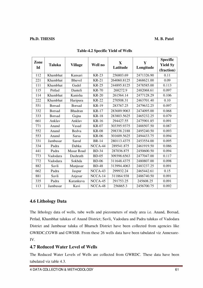
4.5 Specific Yield ‘Sy’ of Wells in an Unconfined Aquifer
Specific yields have been approximated by critically studying aquifer characteristics of study
area and various reference studies, reports and manuals on this area. This data is presented in
table 4.2
Ph.D. THESIS M. B. Patel
4 DATA COLLECTION & METHODOLOGY 61
Table-4.2 Specific Yield of Wells
Zone
Id Taluka Village Well no
X
Latitude
Y
Longitude
Specific
Yield Sy
(fraction)
112 Khambhat Kansari KR-23 256803.69 2471326.90 0.11
221 Khambhat Bhuvel KR-21 264060.8125 2468621.00 0.09
111 Khambhat Gudel KR-25 244895.8125 2478585.00 0.113
115 Petlad Danteli KR-70 268272.9 2482068.61 0.097
114 Khambhat Kanisha KR-20 261564.14 2477128.29 0.106
222 Khambhat Haripura KR-22 270508.31 2463701.40 0.10
551 Borsad Borsad KR-19 283767.25 2479632.25 0.097
332 Borsad Bhadran KR-17 283689.9063 2474095.00 0.068
333 Borsad Gajna KR-18 283803.5625 2465232.25 0.079
661 Anklav Anklav KR-16 294427.55 2475901.85 0.091
771 Anand Vasad KR-07 303395.9375 2488507.50 0.087
552 Anand Bedva KR-08 298338.2188 2495240.50 0.093
553 Anand Sarsa KR-06 301609.5625 2494433.75 0.094
331 Jambusar Sarod BR-14 280113.4375 2453554.00 0.095
334 Padra Dabka NCCA-44 289541.875 2461919.50 0.086
441 Padra Masar Road BD-34 287036.875 2450600.50 0.094
773 Vadodara Dashrath BD-05 309398.6563 2477047.00 0.117
772 Vadodara Sokhda BD-06 311648.4375 2480807.00 0.098
882 Savli Manjusar BD-48 313994.4063 2483237.25 0.091
662 Padra Jaspur NCCA-43 299932.24 2465442.61 0.15
881 Savli Anjesar NCCA-14 311864.938 2486740.50 0.091
335 Padra Karankuva NCCA-45 291753.25 245608.25 0.091
113 Jambusar Kavi NCCA-48 256865.3 2456700.75 0.092
4.6 Lithology Data
The lithology data of wells, tube wells and piezometers of study area i.e. Anand, Borsad,
Petlad, Khambhat talukas of Anand District; Savli, Vadodara and Padra talukas of Vadodara
District and Jambusar taluka of Bharuch District have been collected from agencies like
GWRDC,CGWB and GWSSB. From these 26 wells data have been tabulated viz Annexure-
IV.
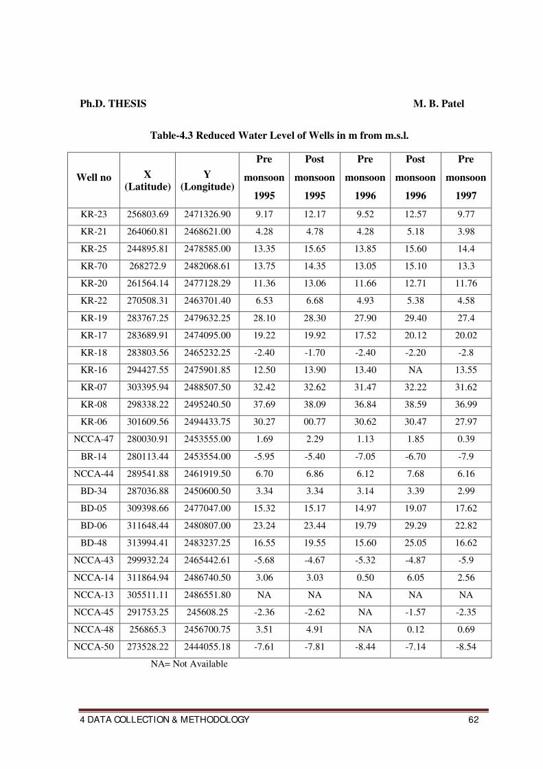
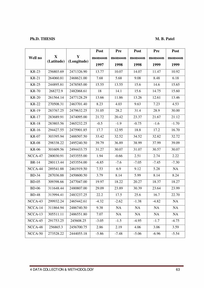
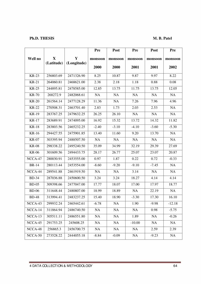
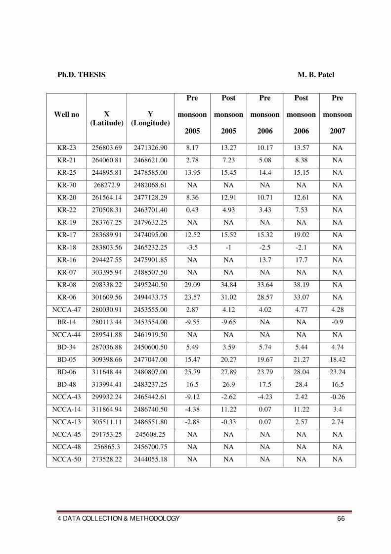
4.7 Reduced Water Level of Wells
The Reduced Water Levels of Wells are collected from GWRDC. These data have been
tabulated viz table 4.3.
Ph.D. THESIS M. B. Patel
4 DATA COLLECTION & METHODOLOGY 62
Table-4.3 Reduced Water Level of Wells in m from m.s.l.
Well no X
(Latitude)
Y
(Longitude)
Pre
monsoon
1995
Post
monsoon
1995
Pre
monsoon
1996
Post
monsoon
1996
Pre
monsoon
1997
KR-23 256803.69 2471326.90 9.17 12.17 9.52 12.57 9.77
KR-21 264060.81 2468621.00 4.28 4.78 4.28 5.18 3.98
KR-25 244895.81 2478585.00 13.35 15.65 13.85 15.60 14.4
KR-70 268272.9 2482068.61 13.75 14.35 13.05 15.10 13.3
KR-20 261564.14 2477128.29 11.36 13.06 11.66 12.71 11.76
KR-22 270508.31 2463701.40 6.53 6.68 4.93 5.38 4.58
KR-19 283767.25 2479632.25 28.10 28.30 27.90 29.40 27.4
KR-17 283689.91 2474095.00 19.22 19.92 17.52 20.12 20.02
KR-18 283803.56 2465232.25 -2.40 -1.70 -2.40 -2.20 -2.8
KR-16 294427.55 2475901.85 12.50 13.90 13.40 NA 13.55
KR-07 303395.94 2488507.50 32.42 32.62 31.47 32.22 31.62
KR-08 298338.22 2495240.50 37.69 38.09 36.84 38.59 36.99
KR-06 301609.56 2494433.75 30.27 00.77 30.62 30.47 27.97
NCCA-47 280030.91 2453555.00 1.69 2.29 1.13 1.85 0.39
BR-14 280113.44 2453554.00 -5.95 -5.40 -7.05 -6.70 -7.9
NCCA-44 289541.88 2461919.50 6.70 6.86 6.12 7.68 6.16
BD-34 287036.88 2450600.50 3.34 3.34 3.14 3.39 2.99
BD-05 309398.66 2477047.00 15.32 15.17 14.97 19.07 17.62
BD-06 311648.44 2480807.00 23.24 23.44 19.79 29.29 22.82
BD-48 313994.41 2483237.25 16.55 19.55 15.60 25.05 16.62
NCCA-43 299932.24 2465442.61 -5.68 -4.67 -5.32 -4.87 -5.9
NCCA-14 311864.94 2486740.50 3.06 3.03 0.50 6.05 2.56
NCCA-13 305511.11 2486551.80 NA NA NA NA NA
NCCA-45 291753.25 245608.25 -2.36 -2.62 NA -1.57 -2.35
NCCA-48 256865.3 2456700.75 3.51 4.91 NA 0.12 0.69
NCCA-50 273528.22 2444055.18 -7.61 -7.81 -8.44 -7.14 -8.54
NA= Not Available
Ph.D. THESIS M. B. Patel
4 DATA COLLECTION & METHODOLOGY 63
Well no X
(Latitude)
Y
(Longitude)
Post
monsoon
1997
Pre
monsoon
1998
Post
monsoon
1998
Pre
monsoon
1999
Post
monsoon
1999
KR-23 256803.69 2471326.90 13.77 10.07 14.07 11.47 10.92
KR-21 264060.81 2468621.00 7.68 5.68 9.08 8.48 6.18
KR-25 244895.81 2478585.00 15.55 13.55 15.6 14.6 15.65
KR-70 268272.9 2482068.61 18 14.1 15.6 14.75 15.60
KR-20 261564.14 2477128.29 13.66 11.86 13.26 12.61 13.46
KR-22 270508.31 2463701.40 8.23 4.03 9.63 7.23 4.53
KR-19 283767.25 2479632.25 31.05 28.2 31.4 28.9 30.00
KR-17 283689.91 2474095.00 21.72 20.42 23.37 21.67 21.12
KR-18 283803.56 2465232.25 -0.5 -1.9 -0.75 -1.6 -1.70
KR-16 294427.55 2475901.85 17.7 12.95 18.8 17.2 16.70
KR-07 303395.94 2488507.50 33.42 32.52 34.52 32.82 32.72
KR-08 298338.22 2495240.50 39.79 36.89 38.99 37.99 39.09
KR-06 301609.56 2494433.75 31.27 30.07 31.07 30.57 30.07
NCCA-47 280030.91 2453555.00 1.94 -0.66 2.51 2.74 2.22
BR-14 280113.44 2453554.00 -6.85 -7.6 -7.05 -7.45 -7.30
NCCA-44 289541.88 2461919.50 7.53 6.9 9.12 5.28 NA
BD-34 287036.88 2450600.50 3.79 8.14 5.99 8.14 8.24
BD-05 309398.66 2477047.00 19.97 18.22 20.27 18.37 18.27
BD-06 311648.44 2480807.00 29.09 23.89 30.39 23.64 23.99
BD-48 313994.41 2483237.25 22.2 17.5 25.6 16.7 22.70
NCCA-43 299932.24 2465442.61 -4.32 -2.62 -1.38 -4.82 NA
NCCA-14 311864.94 2486740.50 9.38 NA NA NA NA
NCCA-13 305511.11 2486551.80 7.07 NA NA NA NA
NCCA-45 291753.25 245608.25 -3.05 -1.5 -4.95 -1.7 -4.75
NCCA-48 256865.3 2456700.75 2.86 2.19 4.06 3.06 3.59
NCCA-50 273528.22 2444055.18 -5.86 -7.48 -5.06 -6.96 -5.54
Ph.D. THESIS M. B. Patel
4 DATA COLLECTION & METHODOLOGY 64
Well no X
(Latitude)
Y
(Longitude)
Pre
monsoon
2000
Post
monsoon
2000
Pre
monsoon
2001
Post
monsoon
2001
Pre
monsoon
2002
KR-23 256803.69 2471326.90 8.25 10.87 9.87 9.97 8.22
KR-21 264060.81 2468621.00 2.38 2.18 1.18 0.88 0.08
KR-25 244895.81 2478585.00 12.85 13.75 11.75 13.75 12.05
KR-70 268272.9 2482068.61 NA NA NA NA NA
KR-20 261564.14 2477128.29 11.36 NA 7.26 7.96 4.96
KR-22 270508.31 2463701.40 2.83 1.73 2.03 2.53 NA
KR-19 283767.25 2479632.25 26.25 26.10 NA NA NA
KR-17 283689.91 2474095.00 16.92 15.32 13.72 14.32 11.82
KR-18 283803.56 2465232.25 -2.40 -3.10 -4.10 -3.60 -5.30
KR-16 294427.55 2475901.85 13.40 11.60 9.20 13.70 NA
KR-07 303395.94 2488507.50 NA NA NA NA NA
KR-08 298338.22 2495240.50 35.09 34.99 32.19 29.39 27.69
KR-06 301609.56 2494433.75 28.17 26.77 25.07 23.07 20.87
NCCA-47 280030.91 2453555.00 0.97 1.87 0.22 0.72 -0.33
BR-14 280113.44 2453554.00 -8.60 -9.20 -9.10 -7.45 NA
NCCA-44 289541.88 2461919.50 NA NA 3.14 NA NA
BD-34 287036.88 2450600.50 3.24 3.24 18.27 4.14 4.14
BD-05 309398.66 2477047.00 17.77 18.07 17.00 17.97 18.77
BD-06 311648.44 2480807.00 18.99 18.89 NA 22.19 NA
BD-48 313994.41 2483237.25 15.40 18.90 -3.30 17.30 16.10
NCCA-43 299932.24 2465442.61 -6.78 NA 1.90 -9.98 -12.18
NCCA-14 311864.94 2486740.50 NA NA NA 0.98 -5.75
NCCA-13 305511.11 2486551.80 NA NA 1.89 NA -0.26
NCCA-45 291753.25 245608.25 NA NA -10.00 NA NA
NCCA-48 256865.3 2456700.75 NA NA NA 2.59 2.39
NCCA-50 273528.22 2444055.18 -8.84 -0.09 NA -9.23 NA

Ph.D. THESIS M. B. Patel
4 DATA COLLECTION & METHODOLOGY 65
Well no X
(Latitude)
Y
(Longitude)
Post
monsoon
2002
Pre
monsoon
2003
Post
monsoon
2003
Pre
monsoon
2004
Post
monsoon
2004
KR-23 256803.69 2471326.90 9.87 7.67 10.47 8.72 10.57
KR-21 264060.81 2468621.00 2.38 2.38 8.18 5.48 7.38
KR-25 244895.81 2478585.00 13.95 10.5 14.85 14.55 15.65
KR-70 268272.9 2482068.61 NA NA NA NA NA
KR-20 261564.14 2477128.29 7.76 5.06 12.06 8.51 12.36
KR-22 270508.31 2463701.40 2.03 0.33 4.53 2.48 1.33
KR-19 283767.25 2479632.25 NA NA NA NA NA
KR-17 283689.91 2474095.00 12.42 10.02 11.12 10.92 12.02
KR-18 283803.56 2465232.25 -3.80 -7.9 -1.6 -3.3 -1.5
KR-16 294427.55 2475901.85 NA NA NA NA NA
KR-07 303395.94 2488507.50 NA NA NA NA NA
KR-08 298338.22 2495240.50 28.39 27.19 29.59 29.34 31.39
KR-06 301609.56 2494433.75 22.47 21.37 24.97 24.27 27.97
NCCA-47 280030.91 2453555.00 0.39 -0.88 2.1 2.12 2.62
BR-14 280113.44 2453554.00 -8.85 NA -8.6 -9.1 -9.1
NCCA-44 289541.88 2461919.50 NA NA NA NA NA
BD-34 287036.88 2450600.50 4.34 5.89 3.24 3.14 4.44
BD-05 309398.66 2477047.00 17.97 15.97 19.17 17.47 19.57
BD-06 311648.44 2480807.00 NA 16.79 23.19 21.64 30.29
BD-48 313994.41 2483237.25 20.70 16.8 19.5 17.2 23.9
NCCA-43 299932.24 2465442.61 -11.14 -16.75 -10.38 -11.08 -9.08
NCCA-14 311864.94 2486740.50 2.75 -4.82 7.42 -2.58 6.72
NCCA-13 305511.11 2486551.80 0.00 -10.03 -2.58 -3.33 -1.78
NCCA-45 291753.25 245608.25 NA NA NA NA NA
NCCA-48 256865.3 2456700.75 2.72 1.94 3.09 2.74 3.24
NCCA-50 273528.22 2444055.18 NA NA NA NA NA
Ph.D. THESIS M. B. Patel
4 DATA COLLECTION & METHODOLOGY 66
Well no X
(Latitude)
Y
(Longitude)
Pre
monsoon
2005
Post
monsoon
2005
Pre
monsoon
2006
Post
monsoon
2006
Pre
monsoon
2007
KR-23 256803.69 2471326.90 8.17 13.27 10.17 13.57 NA
KR-21 264060.81 2468621.00 2.78 7.23 5.08 8.38 NA
KR-25 244895.81 2478585.00 13.95 15.45 14.4 15.15 NA
KR-70 268272.9 2482068.61 NA NA NA NA NA
KR-20 261564.14 2477128.29 8.36 12.91 10.71 12.61 NA
KR-22 270508.31 2463701.40 0.43 4.93 3.43 7.53 NA
KR-19 283767.25 2479632.25 NA NA NA NA NA
KR-17 283689.91 2474095.00 12.52 15.52 15.32 19.02 NA
KR-18 283803.56 2465232.25 -3.5 -1 -2.5 -2.1 NA
KR-16 294427.55 2475901.85 NA NA 13.7 17.7 NA
KR-07 303395.94 2488507.50 NA NA NA NA NA
KR-08 298338.22 2495240.50 29.09 34.84 33.64 38.19 NA
KR-06 301609.56 2494433.75 23.57 31.02 28.57 33.07 NA
NCCA-47 280030.91 2453555.00 2.87 4.12 4.02 4.77 4.28
BR-14 280113.44 2453554.00 -9.55 -9.65 NA NA -0.9
NCCA-44 289541.88 2461919.50 NA NA NA NA NA
BD-34 287036.88 2450600.50 5.49 3.59 5.74 5.44 4.74
BD-05 309398.66 2477047.00 15.47 20.27 19.67 21.27 18.42
BD-06 311648.44 2480807.00 25.79 27.89 23.79 28.04 23.24
BD-48 313994.41 2483237.25 16.5 26.9 17.5 28.4 16.5
NCCA-43 299932.24 2465442.61 -9.12 -2.62 -4.23 2.42 -0.26
NCCA-14 311864.94 2486740.50 -4.38 11.22 0.07 11.22 3.4
NCCA-13 305511.11 2486551.80 -2.88 -0.33 0.07 2.57 2.74
NCCA-45 291753.25 245608.25 NA NA NA NA NA
NCCA-48 256865.3 2456700.75 NA NA NA NA NA
NCCA-50 273528.22 2444055.18 NA NA NA NA NA
Ph.D. THESIS M. B. Patel
4 DATA COLLECTION & METHODOLOGY 67
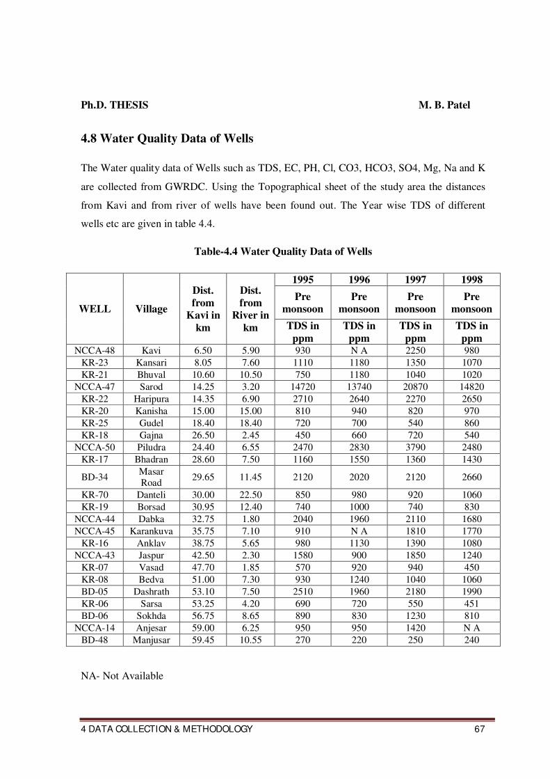
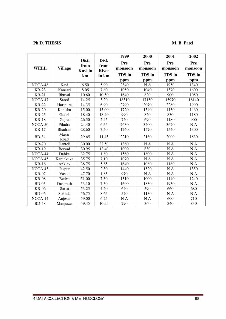
4.8 Water Quality Data of Wells
The Water quality data of Wells such as TDS, EC, PH, Cl, CO3, HCO3, SO4, Mg, Na and K
are collected from GWRDC. Using the Topographical sheet of the study area the distances
from Kavi and from river of wells have been found out. The Year wise TDS of different
wells etc are given in table 4.4.
Table-4.4 Water Quality Data of Wells
WELL Village
Dist.
from
Kavi in
km
Dist.
from
River in
km
1995 1996 1997 1998
Pre
monsoon
Pre
monsoon
Pre
monsoon
Pre
monsoon
TDS in
ppm
TDS in
ppm
TDS in
ppm
TDS in
ppm NCCA-48 Kavi 6.50 5.90 930 N A 2250 980
KR-23 Kansari 8.05 7.60 1110 1180 1350 1070
KR-21 Bhuval 10.60 10.50 750 1180 1040 1020
NCCA-47 Sarod 14.25 3.20 14720 13740 20870 14820
KR-22 Haripura 14.35 6.90 2710 2640 2270 2650
KR-20 Kanisha 15.00 15.00 810 940 820 970
KR-25 Gudel 18.40 18.40 720 700 540 860
KR-18 Gajna 26.50 2.45 450 660 720 540
NCCA-50 Piludra 24.40 6.55 2470 2830 3790 2480
KR-17 Bhadran 28.60 7.50 1160 1550 1360 1430
BD-34 Masar Road
29.65 11.45 2120 2020 2120 2660
KR-70 Danteli 30.00 22.50 850 980 920 1060
KR-19 Borsad 30.95 12.40 740 1000 740 830
NCCA-44 Dabka 32.75 1.80 2040 1960 2110 1680
NCCA-45 Karankuva 35.75 7.10 910 N A 1810 1770
KR-16 Anklav 38.75 5.65 980 1130 1390 1080
NCCA-43 Jaspur 42.50 2.30 1580 900 1850 1240
KR-07 Vasad 47.70 1.85 570 920 940 450
KR-08 Bedva 51.00 7.30 930 1240 1040 1060
BD-05 Dashrath 53.10 7.50 2510 1960 2180 1990
KR-06 Sarsa 53.25 4.20 690 720 550 451
BD-06 Sokhda 56.75 8.65 890 830 1230 810
NCCA-14 Anjesar 59.00 6.25 950 950 1420 N A
BD-48 Manjusar 59.45 10.55 270 220 250 240
NA- Not Available
Ph.D. THESIS M. B. Patel
4 DATA COLLECTION & METHODOLOGY 68
WELL Village
Dist.
from
Kavi in
km
Dist.
from
River
in km
1999 2000 2001 2002
Pre
monsoon
Pre
monsoon
Pre
monsoon
Pre
monsoon
TDS in
ppm
TDS in
ppm
TDS in
ppm
TDS in
ppm NCCA-48 Kavi 6.50 5.90 2340 N A 1950 1340
KR-23 Kansari 8.05 7.60 1050 1040 1370 1600
KR-21 Bhuval 10.60 10.50 1640 820 900 1080
NCCA-47 Sarod 14.25 3.20 18310 17150 15970 18140
KR-22 Haripura 14.35 6.90 2790 2070 2280 1990
KR-20 Kanisha 15.00 15.00 1720 1540 1130 1460
KR-25 Gudel 18.40 18.40 990 820 830 1180
KR-18 Gajna 26.50 2.45 720 690 1180 900
NCCA-50 Piludra 24.40 6.55 2630 3400 3620 N A
KR-17 Bhadran 28.60 7.50 1760 1470 1540 1300
BD-34 Masar
Road 29.65 11.45 2210 2160 2000 1830
KR-70 Danteli 30.00 22.50 1360 N A N A N A
KR-19 Borsad 30.95 12.40 1090 830 N A N A
NCCA-44 Dabka 32.75 1.80 1560 1800 N A N A
NCCA-45 Karankuva 35.75 7.10 1070 N A N A N A
KR-16 Anklav 38.75 5.65 1640 1080 1180 N A
NCCA-43 Jaspur 42.50 2.30 1440 1520 N A 1350
KR-07 Vasad 47.70 1.85 970 N A N A N A
KR-08 Bedva 51.00 7.30 1310 1000 1140 1240
BD-05 Dashrath 53.10 7.50 1600 1830 1930 N A
KR-06 Sarsa 53.25 4.20 640 590 660 680
BD-06 Sokhda 56.75 8.65 520 1130 N A N A
NCCA-14 Anjesar 59.00 6.25 N A N A 600 710
BD-48 Manjusar 59.45 10.55 290 360 340 830

Ph.D. THESIS M. B. Patel
4 DATA COLLECTION & METHODOLOGY 69
WELL Village
Dist.
from
Kavi in
km
Dist.
from
River
in km
2003 2004 2005 2006
Pre
monsoon
Pre
monsoon
Pre
monsoon
Pre
monsoon
TDS in
ppm
TDS in
ppm
TDS in
ppm
TDS in
ppm NCCA-48 Kavi 6.50 5.90 1170 N A N A N A
KR-23 Kansari 8.05 7.60 1460 1820 1420 1190
KR-21 Bhuval 10.60 10.50 1080 1360 1080 970
NCCA-47 Sarod 14.25 3.20 17890 20130 15970 18110
KR-22 Haripura 14.35 6.90 1760 1490 2260 2150
KR-20 Kanisha 15.00 15.00 1470 2080 1290 1070
KR-25 Gudel 18.40 18.40 1850 630 1040 860
KR-18 Gajna 26.50 2.45 1310 740 1080 930
NCCA-50 Piludra 24.40 6.55 N A N A N A N A
KR-17 Bhadran 28.60 7.50 1330 1600 1570 1690
BD-34 Masar Road 29.65 11.45 2340 2080 2150 3200
KR-70 Danteli 30.00 22.50 N A N A N A N A
KR-19 Borsad 30.95 12.40 N A N A N A N A
NCCA-44 Dabka 32.75 1.80 N A N A N A N A
NCCA-45 Karankuva 35.75 7.10 N A N A N A N A
KR-16 Anklav 38.75 5.65 N A N A N A 1160
NCCA-43 Jaspur 42.50 2.30 930 960 950 N A
KR-07 Vasad 47.70 1.85 N A N A N A N A
KR-08 Bedva 51.00 7.30 1000 1030 1190 1380
BD-05 Dashrath 53.10 7.50 2170 400 1830 2010
KR-06 Sarsa 53.25 4.20 440 740 750 630
BD-06 Sokhda 56.75 8.65 990 790 870 600
NCCA-14 Anjesar 59.00 6.25 470 590 510 370
BD-48 Manjusar 59.45 10.55 N A 350 320 250
Ph.D. THESIS M. B. Patel
4 DATA COLLECTION & METHODOLOGY 70
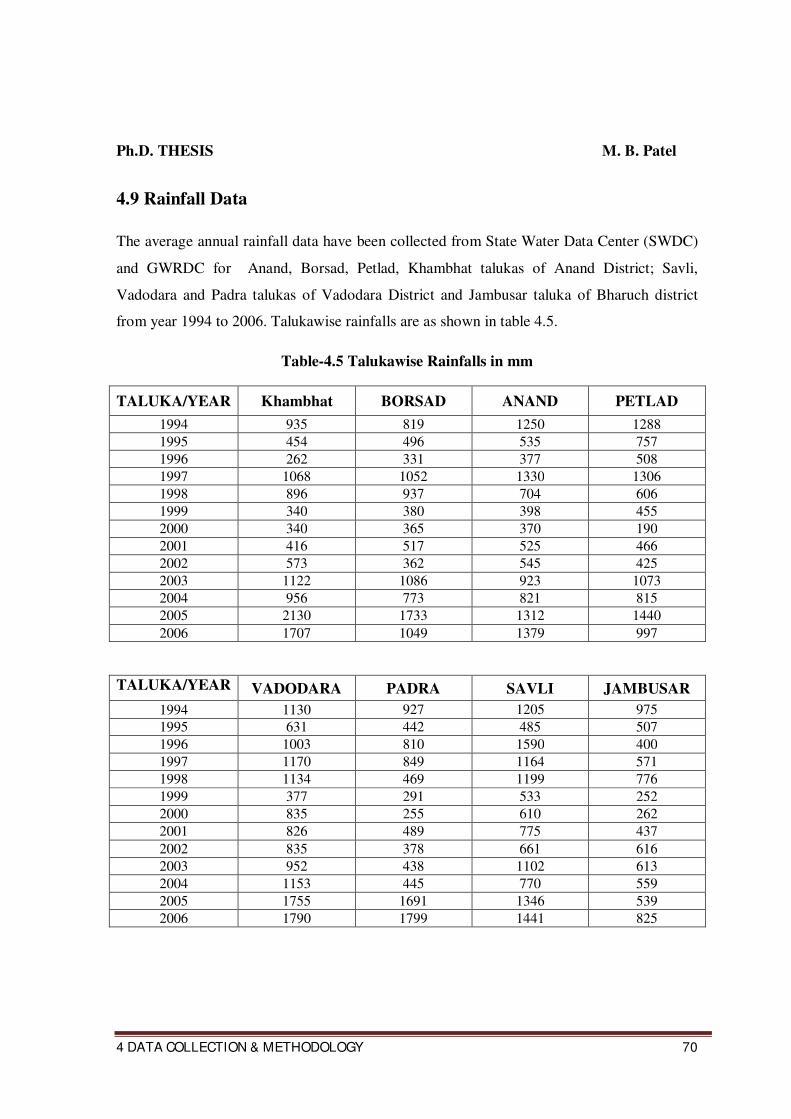
4.9 Rainfall Data
The average annual rainfall data have been collected from State Water Data Center (SWDC)
and GWRDC for Anand, Borsad, Petlad, Khambhat talukas of Anand District; Savli,
Vadodara and Padra talukas of Vadodara District and Jambusar taluka of Bharuch district
from year 1994 to 2006. Talukawise rainfalls are as shown in table 4.5.
Table-4.5 Talukawise Rainfalls in mm
TALUKA/YEAR Khambhat BORSAD ANAND PETLAD
1994 935 819 1250 1288
1995 454 496 535 757
1996 262 331 377 508
1997 1068 1052 1330 1306
1998 896 937 704 606
1999 340 380 398 455
2000 340 365 370 190
2001 416 517 525 466
2002 573 362 545 425
2003 1122 1086 923 1073
2004 956 773 821 815
2005 2130 1733 1312 1440
2006 1707 1049 1379 997
TALUKA/YEAR VADODARA PADRA SAVLI JAMBUSAR
1994 1130 927 1205 975
1995 631 442 485 507
1996 1003 810 1590 400
1997 1170 849 1164 571
1998 1134 469 1199 776
1999 377 291 533 252
2000 835 255 610 262
2001 826 489 775 437
2002 835 378 661 616
2003 952 438 1102 613
2004 1153 445 770 559
2005 1755 1691 1346 539
2006 1790 1799 1441 825
Ph.D. THESIS M. B. Patel
4 DATA COLLECTION & METHODOLOGY 71
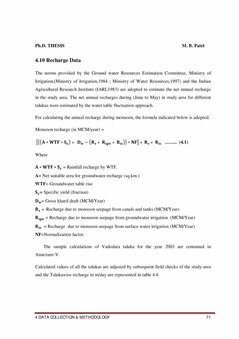
4.10 Recharge Data
The norms provided by the Ground water Resources Estimation Committee, Ministry of
Irrigation,(Ministry of Irrigation,1984 ; Ministry of Water Resources,1997) and the Indian
Agricultural Research Institute (IARI,1983) are adopted to estimate the net annual recharge
in the study area. The net annual recharges during (June to May) in study area for different
talukas were estimated by the water table fluctuation approach.
For calculating the annual recharge during monsoon, the formula indicated below is adopted.
Monsoon recharge (in MCM/year) =
∗ ∗ + − + + ∗ + + …….. (4.1)
Where ∗ ∗ = Rainfall recharge by WTF.
A= Net suitable area for groundwater recharge (sq.km.)
WTF= Groundwater table rise
= Specific yield (fraction)
= Gross kharif draft (MCM/Year)
= Recharge due to monsoon seepage from canals and tanks (MCM/Year)
= Recharge due to monsoon seepage from groundwater irrigation (MCM/Year)
= Recharge due to monsoon seepage from surface water irrigation (MCM/Year)
NF=Normalization factor.
The sample calculations of Vadodara taluka for the year 2003 are contained in
Annexure-V.
Calculated values of all the talukas are adjusted by subsequent field checks of the study area
and the Talukawise recharge in m/day are represented in table 4.6
Ph.D. THESIS M. B. Patel
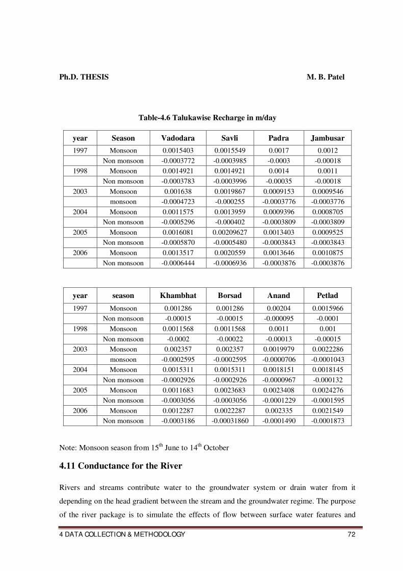
4 DATA COLLECTION & METHODOLOGY 72
Table-4.6 Talukawise Recharge in m/day
year Season Vadodara Savli Padra Jambusar
1997 Monsoon 0.0015403 0.0015549 0.0017 0.0012
Non monsoon -0.0003772 -0.0003985 -0.0003 -0.00018
1998 Monsoon 0.0014921 0.0014921 0.0014 0.0011
Non monsoon -0.0003783 -0.0003996 -0.00035 -0.00018
2003 Monsoon 0.001638 0.0019867 0.0009153 0.0009546
monsoon -0.0004723 -0.000255 -0.0003776 -0.0003776
2004 Monsoon 0.0011575 0.0013959 0.0009396 0.0008705
Non monsoon -0.0005296 -0.000402 -0.0003809 -0.0003809
2005 Monsoon 0.0016081 0.00209627 0.0013403 0.0009525
Non monsoon -0.0005870 -0.0005480 -0.0003843 -0.0003843
2006 Monsoon 0.0013517 0.0020559 0.0013646 0.0010875
Non monsoon -0.0006444 -0.0006936 -0.0003876 -0.0003876
year season Khambhat Borsad Anand Petlad
1997 Monsoon 0.001286 0.001286 0.00204 0.0015966
Non monsoon -0.00015 -0.00015 -0.000095 -0.0001
1998 Monsoon 0.0011568 0.0011568 0.0011 0.001
Non monsoon -0.0002 -0.00022 -0.00013 -0.00015
2003 Monsoon 0.002357 0.002357 0.0019979 0.0022286
monsoon -0.0002595 -0.0002595 -0.0000706 -0.0001043
2004 Monsoon 0.0015311 0.0015311 0.0018151 0.0018145
Non monsoon -0.0002926 -0.0002926 -0.0000967 -0.000132
2005 Monsoon 0.0011683 0.0023683 0.0023408 0.0024276
Non monsoon -0.0003056 -0.0003056 -0.0001229 -0.0001595
2006 Monsoon 0.0012287 0.0022287 0.002335 0.0021549
Non monsoon -0.0003186 -0.00031860 -0.0001490 -0.0001873
Note: Monsoon season from 15th
June to 14th
October
4.11 Conductance for the River
Rivers and streams contribute water to the groundwater system or drain water from it
depending on the head gradient between the stream and the groundwater regime. The purpose
of the river package is to simulate the effects of flow between surface water features and
Ph.D. THESIS M. B. Patel
4 DATA COLLECTION & METHODOLOGY 73
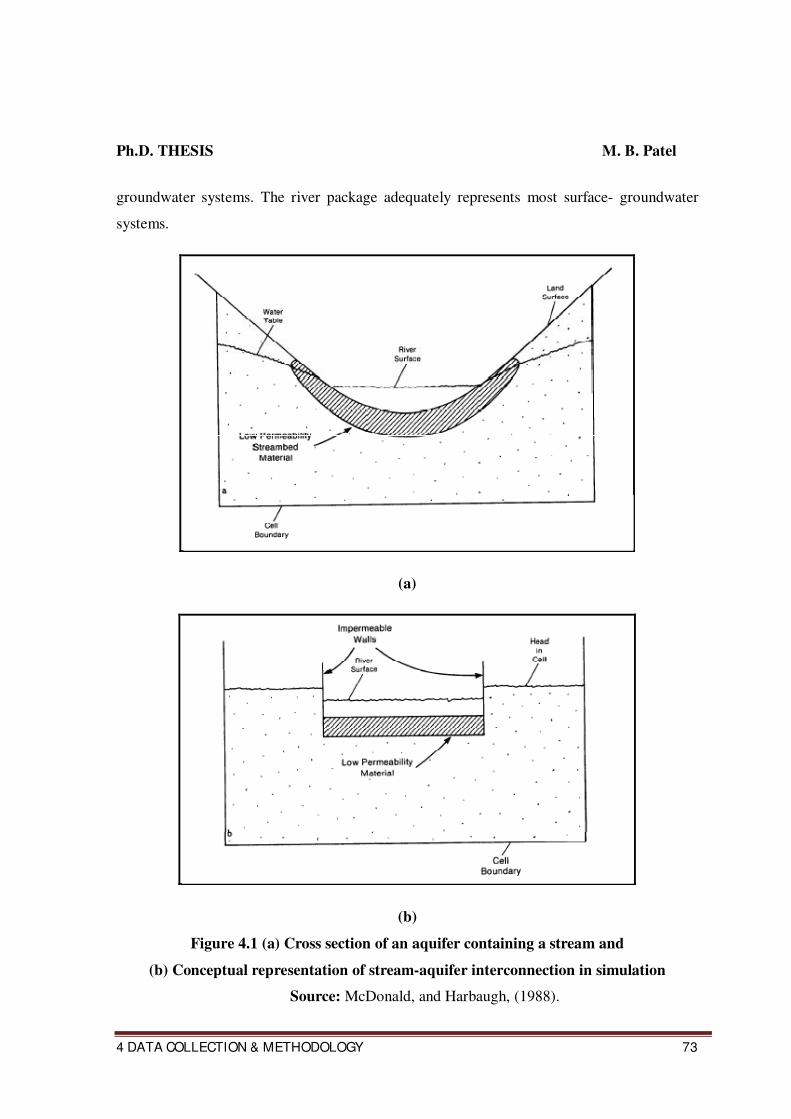
groundwater systems. The river package adequately represents most surface- groundwater
systems.
(a)
(b)
Figure 4.1 (a) Cross section of an aquifer containing a stream and
(b) Conceptual representation of stream-aquifer interconnection in simulation
Source: McDonald, and Harbaugh, (1988).
Ph.D. THESIS M. B. Patel
4 DATA COLLECTION & METHODOLOGY 74
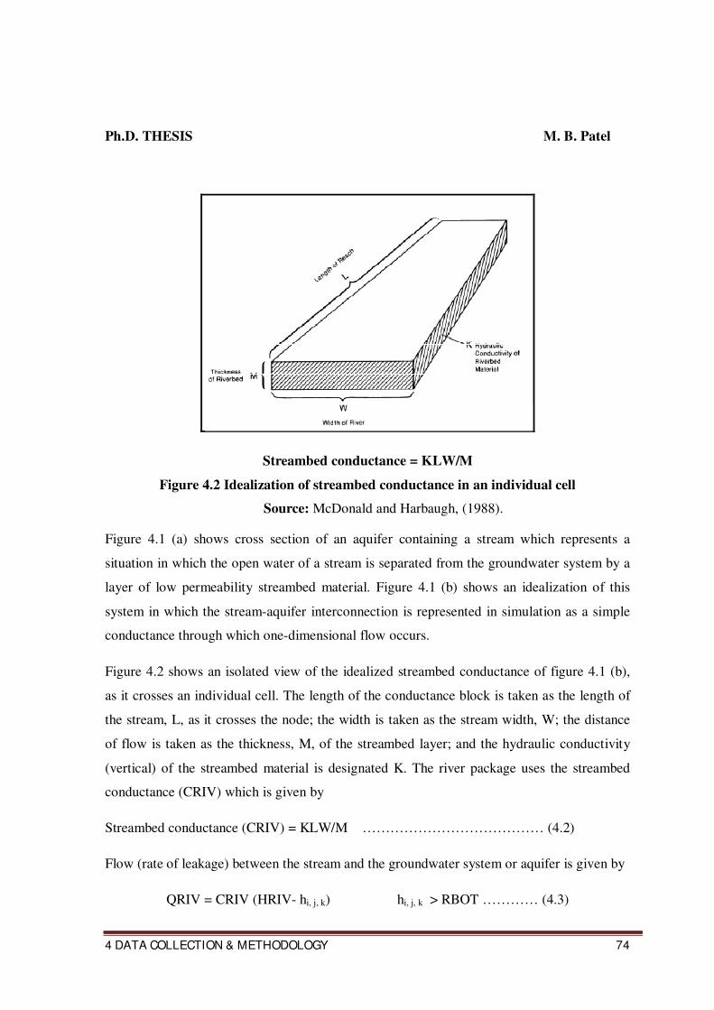
Streambed conductance = KLW/M
Figure 4.2 Idealization of streambed conductance in an individual cell
Source: McDonald and Harbaugh, (1988).
Figure 4.1 (a) shows cross section of an aquifer containing a stream which represents a
situation in which the open water of a stream is separated from the groundwater system by a
layer of low permeability streambed material. Figure 4.1 (b) shows an idealization of this
system in which the stream-aquifer interconnection is represented in simulation as a simple
conductance through which one-dimensional flow occurs.
Figure 4.2 shows an isolated view of the idealized streambed conductance of figure 4.1 (b),
as it crosses an individual cell. The length of the conductance block is taken as the length of
the stream, L, as it crosses the node; the width is taken as the stream width, W; the distance
of flow is taken as the thickness, M, of the streambed layer; and the hydraulic conductivity
(vertical) of the streambed material is designated K. The river package uses the streambed
conductance (CRIV) which is given by
Streambed conductance (CRIV) = KLW/M ………………………………… (4.2)
Flow (rate of leakage) between the stream and the groundwater system or aquifer is given by
QRIV = CRIV (HRIV- hi, j, k) hi, j, k > RBOT ………… (4.3)
Ph.D. THESIS M. B. Patel
4 DATA COLLECTION & METHODOLOGY 75
Where QRIV is the flow between the stream and the aquifer, taken positive if it is directed
into the aquifer; HRIV is the head in the stream; CRIV is the hydraulic conductance of the
stream-aquifer interconnection (KLW/M), hi, j, k is the head at the node in the cell (in the
aquifer) directly underlying the stream reach which corresponds to water table and RBOT is
the bottom of the streambed.
Sometimes the water level (table) in the aquifer has fallen below the bottom of the streambed
layer, leaving an unsaturated interval beneath that layer; if it is assumed that the streambed
layer itself remains saturated, the head at its base will simply be the elevation at that point. If
this elevation is designated RBOT, leakage stabilizes and the flow through the streambed
(QRIV) is given by QRIV = CRIV (HRIV- RBOT), hi, j, k ≤ RBOT ….. (4.4)
If reliable field measurements of stream seepage and associated head difference are available,
they may be used to calculate an effective conductance. Otherwise, a conductance value must
be chosen more or less arbitrarily and adjusted during model calibration (McDonald and
Harbaugh, 1988).
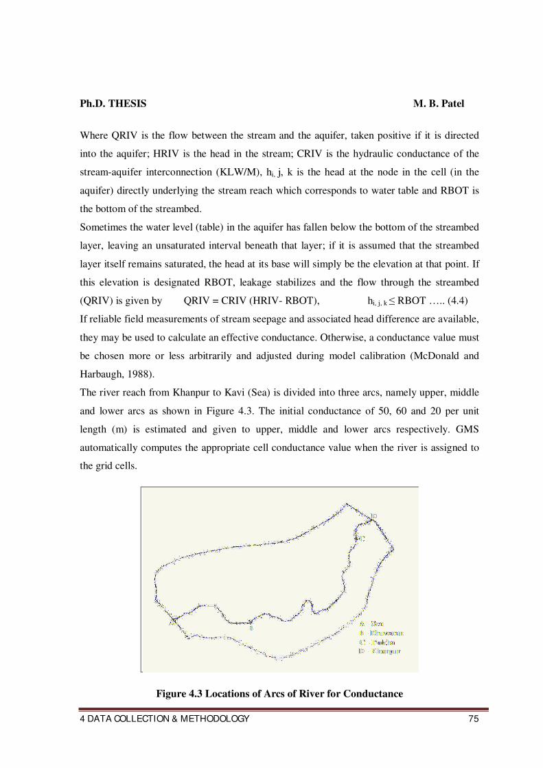
The river reach from Khanpur to Kavi (Sea) is divided into three arcs, namely upper, middle
and lower arcs as shown in Figure 4.3. The initial conductance of 50, 60 and 20 per unit
length (m) is estimated and given to upper, middle and lower arcs respectively. GMS
automatically computes the appropriate cell conductance value when the river is assigned to
the grid cells.
Figure 4.3 Locations of Arcs of River for Conductance
Ph.D. THESIS M. B. Patel
4 DATA COLLECTION & METHODOLOGY 76
4.12 GMS 6.0 Software
The Department of Defense Groundwater Modeling System (GMS) is a comprehensive
graphical user environment for performing groundwater simulations. The entire GMS system
consists of a graphical user interface for ground water modeling (the GMS program) and a
number of pre and post processor of multiple groundwater flow and contaminant transport
analysis codes like MODFLOW, MT3DMS, RT3D, SEAM3D, MODPATH, MODAEM,
SEEP2D, FEMWATER, WASH123D, UTCHEM (Goyal, R. 2003). The GMS interface was
developed by the Environmental Modeling Research Laboratory of Brigham Young
University in partnership with the U.S. Army Engineer Waterways Experiment Station. GMS
was designed as a comprehensive modeling environment. Several types of models are
supported and facilities are provided to share information between different models and data
types. Tools are provided for site characterization, model conceptualization, mesh and grid
generation, geostatistics, and post-processing.
GMS includes a powerful graphical interface to the MODFLOW 2000 model. Most popular
MODFLOW packages are supported. Models can be constructed using either the grid
approach or the conceptual model approach. Numerous options are provided for visualizing
MODFLOW simulation results.
4.12.1 MODFLOW
MODFLOW is a finite-difference modeling program, which simulates groundwater flow in
three dimensions. The code or computer program is written in FORTRAN 77. The program
has a modular format, and consists of a ‘main’ program and a series of highly independent
subroutines called ‘modules’. The modules are grouped into ‘packages’. Each package deals
with a specific feature of the hydrologic system which is to be simulated, such as flow of
rivers or flow into drains, or with a specific method of solving linear equations which
describe the flow system. The division of the program into modules facilitates examination of
each hydrologic feature in the model independently. Another advantage of having the
modular structure is that new options/features could be added to the program without much
change to the existing code.
Ph.D. THESIS M. B. Patel
4 DATA COLLECTION & METHODOLOGY 77
4.12.2 The Conceptual Model Approach
A MODFLOW model can be created in GMS using one of two methods: assigning and
editing values directly to the cells of a grid (the grid approach), or by constructing a high
level representation of the model using feature objects in the Map module and allowing GMS
to automatically assign the values to the cells (the conceptual model approach). Except for
simple problems, the conceptual model approach is typically the most effective.
In GMS, the term conceptual model is used in two different ways. In the generic sense, a
conceptual model is a simplified representation of the site to be modeled including the model
domain, boundary conditions, sources, sinks, and material zones. GMS also has a conceptual
model object, that can be defined in the map module using points, arcs, and polygons. Once
the conceptual model object is defined, a grid can be automatically generated and the
boundary conditions and model parameters are computed and assigned to the proper cells.
This approach to modeling fully automates the majority of the data entry and eliminates the
need for most or all of the tedious cell-by-cell editing traditionally associated with
MODFLOW modeling.
A complete conceptual model object consists of several coverages. One coverage is typically
used to define the sources and sinks such as wells, rivers, lakes, and drains. Coverage (or the
same coverage) is used to define the recharge zones. Other coverages can be used to define
the zones of hydraulic conductivity within each layer. Any number of coverages may be
used, or all these attributes may exist in the same coverage. In addition to the feature data, a
conceptual model may include other data (scatter points, boreholes, solids) to define the layer
elevations. A specialized set of tools for manipulating layer elevation data is provided in
GMS.
4.12.3 Advantages of the Conceptual Model Approach
There are numerous benefits to the conceptual model approach. First of all, the model can be
defined independently of the grid resolution. The modeler does not need to waste valuable
time computing the appropriate conductance to assign to a river cell based on the length of
the river reach within the cell. This type of computation is performed automatically.
Furthermore, transient parameters such as pumping rates for wells can also be assigned
independently of model discretization. Transient parameters are entered as a curve of the

Ph.D. THESIS M. B. Patel
4 DATA COLLECTION & METHODOLOGY 78
stress vs. time. When the conceptual model is converted to the numerical model, the transient
values of the stresses are automatically assigned to the appropriate stress periods. Since the
conceptual model is defined independently of the spatial and temporal discretization of the
numerical model, the conceptual model can be quickly and easily changed and a new
numerical model can be generated in seconds. This allows the modeler to evaluate numerous
alternative conceptual models in the space of time normally required to evaluate one,
resulting in a more accurate and efficient modeling process.
A further advantage of storing attributes with feature objects is that the method of applying
the boundary conditions to the grid cells reduces some of the instability that is inherent in
finite difference models such as MODFLOW and MT3DMS. When the user enters individual
values for heads and elevations, entering cell values one cell at a time can be tedious. It is
also difficult to determine the correct elevation along a river segment at each cell that it
crosses. The temptation is to select small groups of cells in series and apply the same values
to all of the cells in the group. This results in an extreme stair-step condition that can slow or
even prevent convergence of the numerical solver. By using GMS to interpolate values at
locations along a linear boundary condition such as a river, the user insures that there will be
no abrupt changes from cell to cell-thus minimizing the stair-step effect. It also produces a
model with boundary conditions that more accurately represent real world conditions.
4.12.4 Groundwater Flow Equation Used In MODFLOW
The simultaneous equations used by MODFLOW for each finite difference cell is derived
using Darcy’s Law and the law of conservation of mass. The derivation gives a partial
differential equation, which is used by MODFLOW. This partial-differential equation of
groundwater flow used in MODFLOW-2000 is
K + K + K + W = S ………………… (4.5)
Where,
Kxx, Kyy, and Kzz are values of hydraulic conductivity along the x, y, and z coordinate axes,
which are assumed to be parallel to the major axes of hydraulic conductivity (L/T);
h is the potentiometric head (L);
W is a volumetric flux per unit volume representing sources and/or sinks of water, with
W<0.0 for flow out of the ground-water system, and W>0.0 for flow in (T );
Ph.D. THESIS M. B. Patel
4 DATA COLLECTION & METHODOLOGY 79
S is the specific storage of the porous material (L ); and
t is time (T).
Above Equation, when combined with boundary and initial conditions, describes transient
three-dimensional ground-water flow in a heterogeneous and anisotropic medium, provided
that the principal axes of hydraulic conductivity are aligned with the coordinate directions.
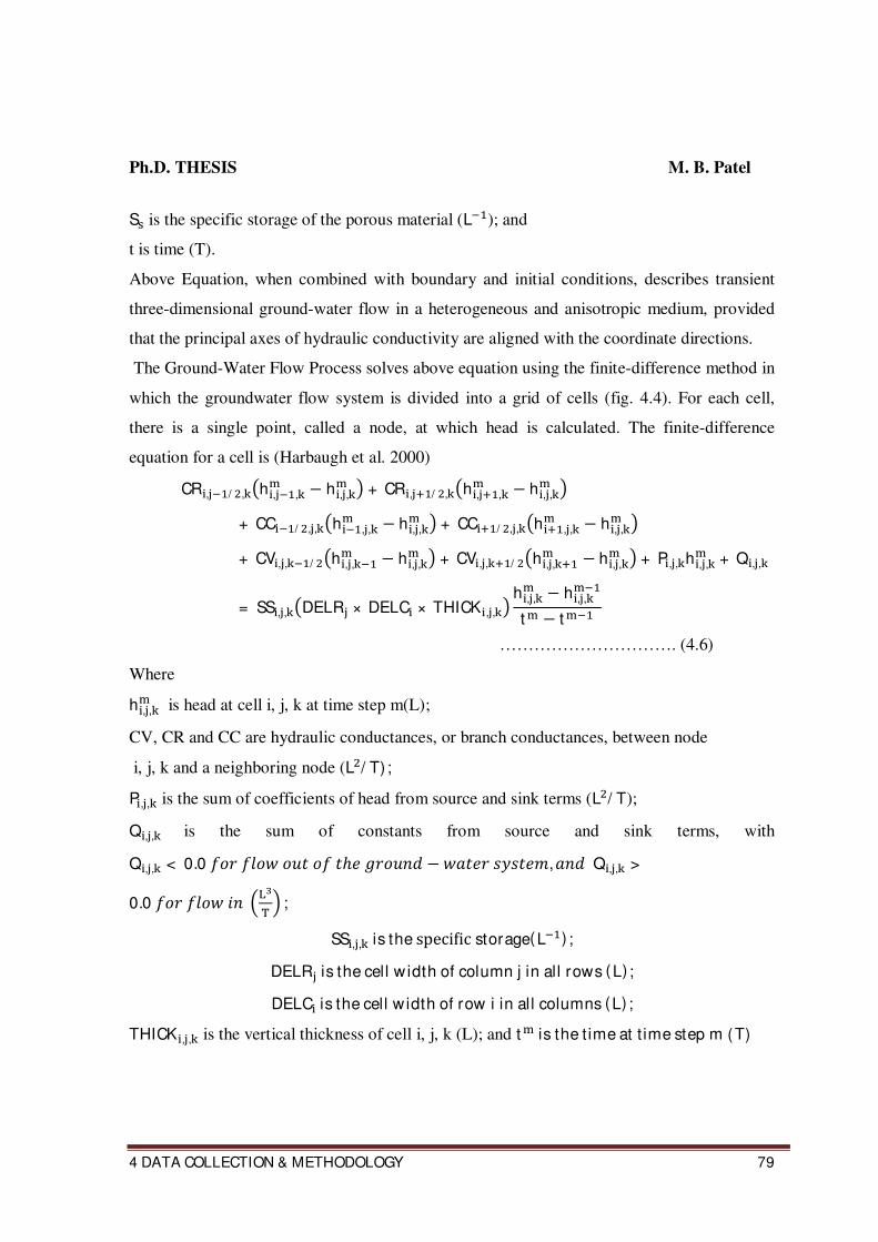
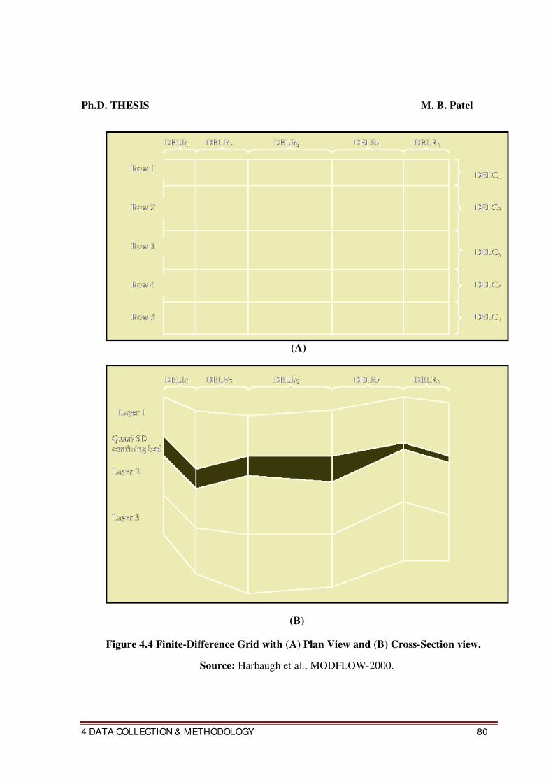
The Ground-Water Flow Process solves above equation using the finite-difference method in
which the groundwater flow system is divided into a grid of cells (fig. 4.4). For each cell,
there is a single point, called a node, at which head is calculated. The finite-difference
equation for a cell is (Harbaugh et al. 2000) CR , / , h , , − h , , + CR , / , h , , − h , , + CC / , , h , , − h , , + CC / , , h , , − h , ,
+ CV , , / h , , − h , , + CV , , / h , , − h , , + P, , h , , + Q , ,
= SS , , DELR × DELC × THICK , ,
h , , − h , ,
t − t
…………………………. (4.6)
Where
h , , is head at cell i, j, k at time step m(L);
CV, CR and CC are hydraulic conductances, or branch conductances, between node
i, j, k and a neighboring node (L / T) ;
P, , is the sum of coefficients of head from source and sink terms (L / T);
Q , , is the sum of constants from source and sink terms, with
Q , , < 0.0 ℎ − , Q , , >
0.0 ;
SS , , isthespeci icstorage(L ) ;
DELR isthecell widthofcolumnjinall rows(L) ;
DELC isthecell widthofrow i inallcolumns(L) ;
THICK , , is the vertical thickness of cell i, j, k (L); and t isthet imeat t imestepm(T)
Ph.D. THESIS M. B. Patel
4 DATA COLLECTION & METHODOLOGY 80
(A)
(B)
Figure 4.4 Finite-Difference Grid with (A) Plan View and (B) Cross-Section view.
Source: Harbaugh et al., MODFLOW-2000.
Ph.D. THESIS M. B. Patel
4 DATA COLLECTION & METHODOLOGY 81
4.13 Groundwater Modeling
Groundwater modeling is a powerful management tool which can serve multiple purposes
such as providing a framework for organizing hydrological data, quantifying the properties
and behavior of the systems and allowing quantitative prediction of the responses of those
systems to externally applied stresses. No other numerical groundwater management tool is
as effective as a 3-dimensional groundwater model. A number of groundwater modeling
studies have been carried out around the World for effective groundwater management. A
digital groundwater model is an idealized representation of a groundwater system and
describes in mathematical language, how the basin would function under various conditions.
It considers relationship among parts of the system and stresses on the system simultaneously
and describes the system studied in concise quantitative terms (ORG, 1982).
Conceptual models describe how water enters an aquifer system, flows through the aquifer
system and leaves the aquifer system. Conceptual models start with simple sketches although
in their final form they may be detailed three dimensional diagrams. Developing a conceptual
model is not straightforward. It is necessary to examine all available data, other information,
visit the area under different climatic conditions and talk to those who have used the aquifer.
Insights can be gained from case studies in similar areas, but there will be always be new
features to identify since every aquifer system has unique features. The conceptual model is
put into a form suitable for modeling. The step includes design of the grid, selecting time
steps, setting boundary, and initial conditions and preliminary selection of values for aquifer
parameters and hydrologic stress.
Perhaps the most demanding task in preparing a numerical model from a conceptual model is
the selection of appropriate values of the aquifer parameters. Inevitably there is insufficient
information. Even if additional fieldwork is carried out, the selection of suitable parameter
values requires skill, experience and judgment. Furthermore, the selection of parameter
values is a time consuming task. Unless it is carried out systematically and thoroughly, a
great deal of rethinking may required in later stages of model refinement. For each parameter
it is advisable to quote the best estimate and arrange which represents the uncertainty.
Numerical models should not have unnecessary complexity in terms of number of layers,
number of mesh divisions and size of time steps. Another issue which requires careful
Ph.D. THESIS M. B. Patel
4 DATA COLLECTION & METHODOLOGY 82
attention is that there are some features which are not conveniently represented in certain
numerical model codes. Refinement of numerical groundwater models when the model code
is run for the first time there are likely to be many differences between field and modeled
values of groundwater heads and flows. First of all there will be differences because of
mistakes in preparing the input data; very careful checks must be made to ensure that the
model boundaries parameter values, inflow and outflow are correctly included in the
numerical model (Rushton, 2003).
A protocol for modeling includes code selection and verification, model design, calibration,
sensitivity analysis and finally prediction (Anderson, 1992).
4.13.1 Assumptions and Considerations in Model Analysis
1. Basin is a single layered unconfined aquifer.
2. An impermeable basement boundary (either the basement is complex or the tertiary
clays) exists at the bottom of aquifer.
3. The storage coefficient (specific yield) is constant with time.
4. Vertical flow components are negligible compared to horizontal flow components.
4.13.2 Construction of the Model for the Study Area
Study area’s Northern and Southern limits are marked by catchment boundary of Mahi basin.
The western limit is determined by the Gulf of Khambhat and in the east the area stretches up
to Khanpur between catchment boundaries of Mahi basin. The study area comprises an area
of 2298.23 sq. km and is enclosed within the North latitude 22°05’06” to 22°33’36” and East
longitude 72°27’18” to 73°13’57”.
The selection of MODFLOW is widely accepted model all over the world and many regional
groundwater modeling studies based on MODFLOW are reported in the literature (Elango
and Senthilkumar (2006), Elango (2009)). It has capabilities to handle unsteady, three
dimensional groundwater flow problems with complex hydrogeogical features. Integration of
MODFLOW in GMS provides calibration utility. Hence GMS software is selected for
present study. Using the software Groundwater Modeling System (GMS 6.0) the Mahi
Ph.D. THESIS M. B. Patel
4 DATA COLLECTION & METHODOLOGY 83
estuarine area has been modeled. The analysis has been carried out using Layer Property
Flow (LPF) package of MODFLOW-2000 (based on Finite Difference Method) in GMS6.0.
4.13.2.1 Base Map Preparation
For base map, a scanned image of study area has been registered in appropriate co-ordinate
system (UTM co-ordinate system) using Arc view software (GIS) and shape (shp) file of this
Mahi estuarine area is established. This shape file is imported to GMS and a base map for
three dimensional groundwater flow model is obtained. Top elevation of Ground Level data
modeling have been taken from Annexure-II.
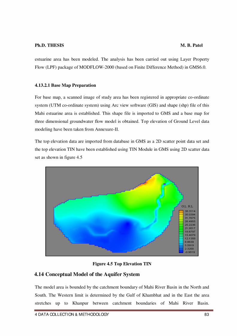
The top elevation data are imported from database in GMS as a 2D scatter point data set and
the top elevation TIN have been established using TIN Module in GMS using 2D scatter data
set as shown in figure 4.5
Figure 4.5 Top Elevation TIN
4.14 Conceptual Model of the Aquifer System
The model area is bounded by the catchment boundary of Mahi River Basin in the North and
South. The Western limit is determined by the Gulf of Khambhat and in the East the area
stretches up to Khanpur between catchment boundaries of Mahi River Basin.
Ph.D. THESIS M. B. Patel
4 DATA COLLECTION & METHODOLOGY 84
The aquifer system of the model area is typical alluvial. Recharge to the aquifer system is
mainly by infiltration of rainfall, seepage from rivers and the drainable surplus from
irrigation. At present the most important discharge component is pumpage from wells for
irrigation. It includes net groundwater recharge zones and other boundaries which can be
represented as head dependent flow boundaries.
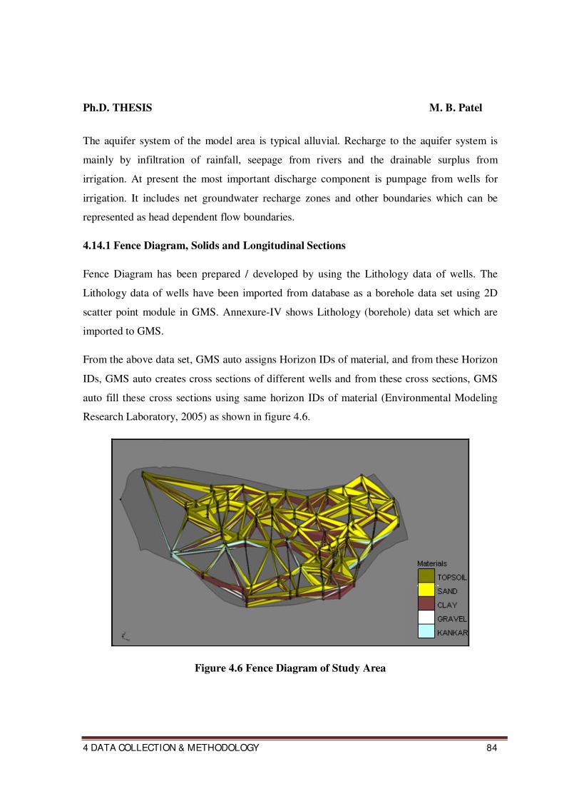
4.14.1 Fence Diagram, Solids and Longitudinal Sections
Fence Diagram has been prepared / developed by using the Lithology data of wells. The
Lithology data of wells have been imported from database as a borehole data set using 2D
scatter point module in GMS. Annexure-IV shows Lithology (borehole) data set which are
imported to GMS.
From the above data set, GMS auto assigns Horizon IDs of material, and from these Horizon
IDs, GMS auto creates cross sections of different wells and from these cross sections, GMS
auto fill these cross sections using same horizon IDs of material (Environmental Modeling
Research Laboratory, 2005) as shown in figure 4.6.
Figure 4.6 Fence Diagram of Study Area

Ph.D. THESIS M. B. Patel
4 DATA COLLECTION & METHODOLOGY 85
From the above cross sections of different wells, The Solid module of GMS is used to
construct three-dimensional models of stratigraphy using solids of study area created is
shown in figure 4.7.
Figure 4.7 Solids of Study Area
Once the three-dimensional model (Solids) is created, cross sections can be cut anywhere on
the model to create Longitudinal Sections. Fig 4.8 shows the three location of longitudinal
sections i.e. along right bank (A-A’), along River (B-B’) and along left bank (C-C’) that have
been cut for longitudinal sections as shown in figure 4.9 to 4.11.

Ph.D. THESIS M. B. Patel
4 DATA COLLECTION & METHODOLOGY 86
Figure 4.8 Three Locations of Longitudinal Section
Figure 4.9 Longitudinal Section Along Right Bank (Section A-A’)
From Kavi (sea) to Khanpur about 85 km U/S of Kavi
Ph.D. THESIS M. B. Patel
4 DATA COLLECTION & METHODOLOGY 87
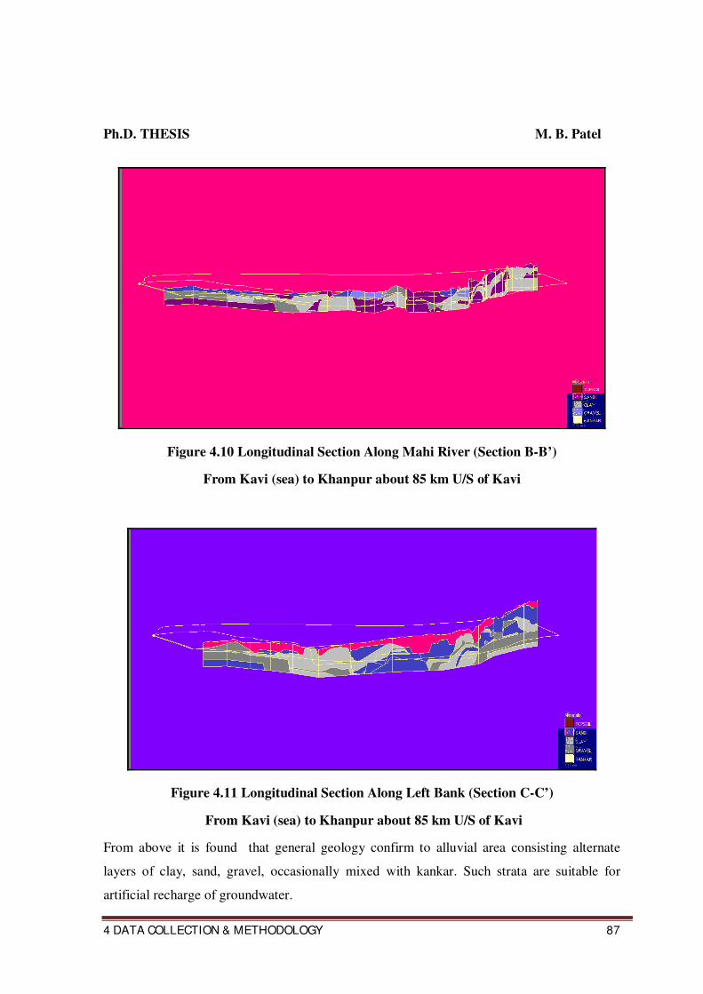
Figure 4.10 Longitudinal Section Along Mahi River (Section B-B’)
From Kavi (sea) to Khanpur about 85 km U/S of Kavi
Figure 4.11 Longitudinal Section Along Left Bank (Section C-C’)
From Kavi (sea) to Khanpur about 85 km U/S of Kavi
From above it is found that general geology confirm to alluvial area consisting alternate
layers of clay, sand, gravel, occasionally mixed with kankar. Such strata are suitable for
artificial recharge of groundwater.
Ph.D. THESIS M. B. Patel
4 DATA COLLECTION & METHODOLOGY 88
4.15 Three Dimensional Model for Present Study
From the detailed study of lithology of wells and previous study reports the aquifer is
considered as unconfined aquifer. As the thickness of unconfined aquifer is very less as
compared to extent of study area (2298.23sq.km), the consideration of single layer
unconfined aquifer in model to be appropriate for study of recharge. Using top elevation TIN
and bottom elevation from Reduced Levels of bottom of wells in unconfined aquifer
Annexure-III the three- dimensional groundwater model (solids) is created for present study.
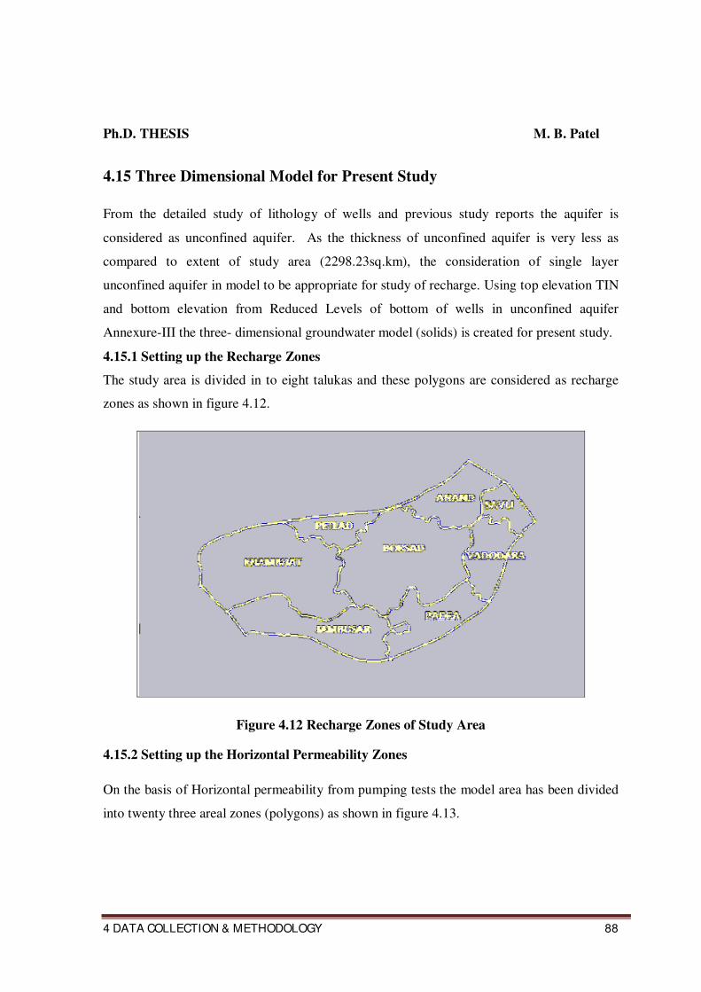
4.15.1 Setting up the Recharge Zones
The study area is divided in to eight talukas and these polygons are considered as recharge
zones as shown in figure 4.12.
Figure 4.12 Recharge Zones of Study Area
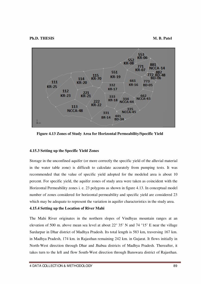
4.15.2 Setting up the Horizontal Permeability Zones
On the basis of Horizontal permeability from pumping tests the model area has been divided
into twenty three areal zones (polygons) as shown in figure 4.13.
Ph.D. THESIS M. B. Patel
4 DATA COLLECTION & METHODOLOGY 89
Figure 4.13 Zones of Study Area for Horizontal Permeability/Specific Yield
4.15.3 Setting up the Specific Yield Zones
Storage in the unconfined aquifer (or more correctly the specific yield of the alluvial material
in the water table zone) is difficult to calculate accurately from pumping tests. It was
recommended that the value of specific yield adopted for the modeled area is about 10
percent. For specific yield, the aquifer zones of study area were taken as coincident with the
Horizontal Permeability zones i. e. 23 polygons as shown in figure 4.13. In conceptual model
number of zones considered for horizontal permeability and specific yield are considered 23
which may be adequate to represent the variation in aquifer characteristics in the study area.
4.15.4 Setting up the Location of River Mahi
The Mahi River originates in the northern slopes of Vindhyas mountain ranges at an
elevation of 500 m. above mean sea level at about 22° 35’ N and 74 °15’ E near the village
Sardarpur in Dhar district of Madhya Pradesh. Its total length is 583 km, traversing 167 km.
in Madhya Pradesh, 174 km. in Rajasthan remaining 242 km. in Gujarat. It flows initially in
North-West direction through Dhar and Jhabua districts of Madhya Pradesh. Thereafter, it
takes turn to the left and flow South-West direction through Banswara district of Rajasthan.
Ph.D. THESIS M. B. Patel
4 DATA COLLECTION & METHODOLOGY 90
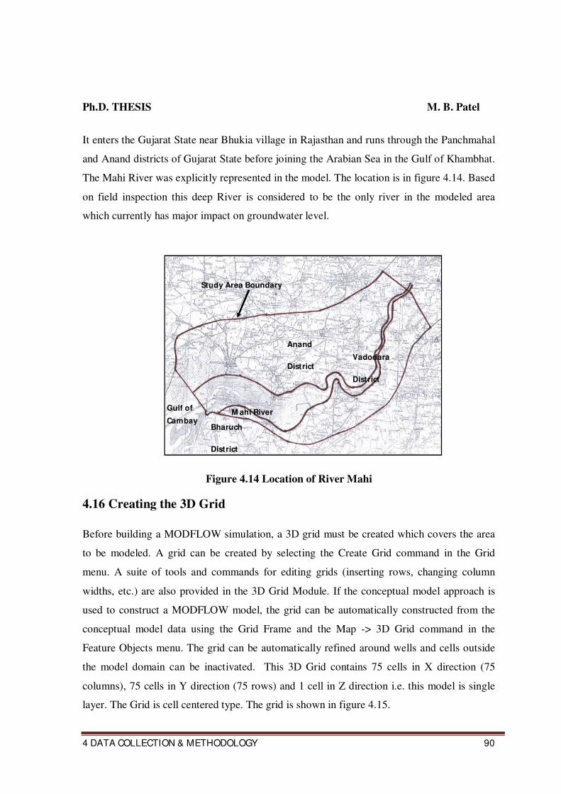
It enters the Gujarat State near Bhukia village in Rajasthan and runs through the Panchmahal
and Anand districts of Gujarat State before joining the Arabian Sea in the Gulf of Khambhat.
The Mahi River was explicitly represented in the model. The location is in figure 4.14. Based
on field inspection this deep River is considered to be the only river in the modeled area
which currently has major impact on groundwater level.
Figure 4.14 Location of River Mahi
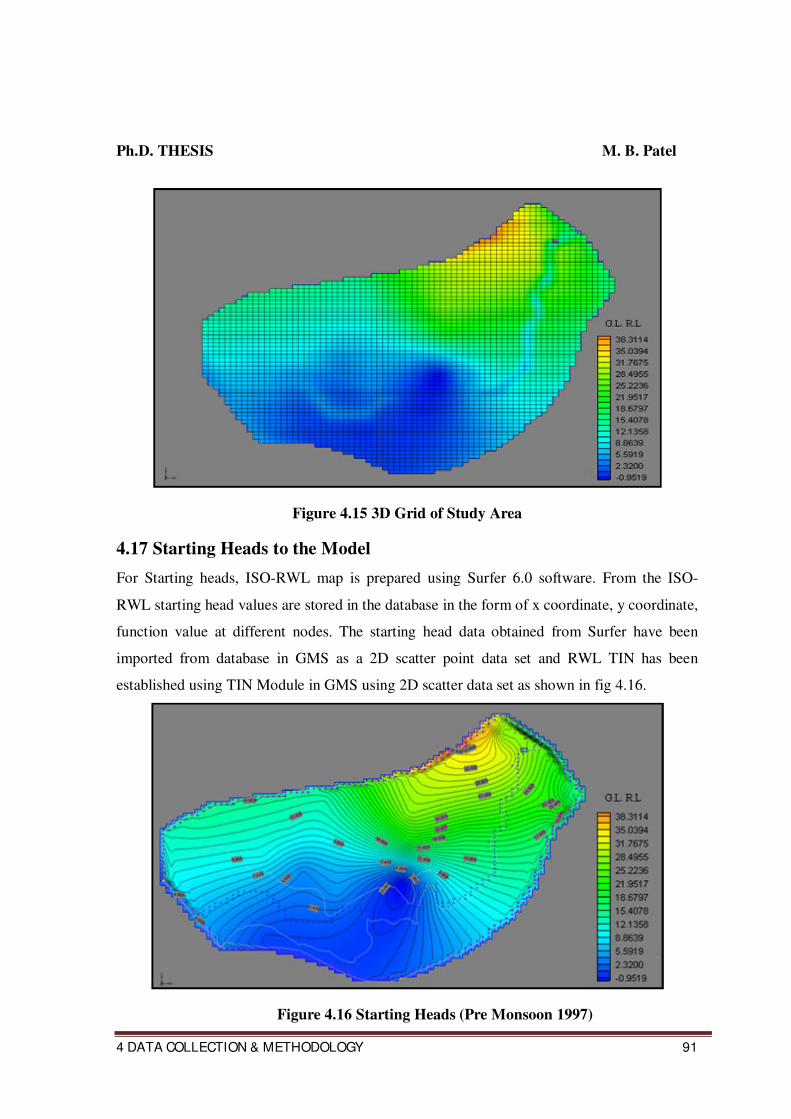
4.16 Creating the 3D Grid
Before building a MODFLOW simulation, a 3D grid must be created which covers the area
to be modeled. A grid can be created by selecting the Create Grid command in the Grid
menu. A suite of tools and commands for editing grids (inserting rows, changing column
widths, etc.) are also provided in the 3D Grid Module. If the conceptual model approach is
used to construct a MODFLOW model, the grid can be automatically constructed from the
conceptual model data using the Grid Frame and the Map -> 3D Grid command in the
Feature Objects menu. The grid can be automatically refined around wells and cells outside
the model domain can be inactivated. This 3D Grid contains 75 cells in X direction (75
columns), 75 cells in Y direction (75 rows) and 1 cell in Z direction i.e. this model is single
layer. The Grid is cell centered type. The grid is shown in figure 4.15.
Study Area Boundary
Anand
District Vadodara
District
Gulf of
Cambay M ahi River
Bharuch
District
Ph.D. THESIS M. B. Patel
4 DATA COLLECTION & METHODOLOGY 91
Figure 4.15 3D Grid of Study Area
4.17 Starting Heads to the Model
For Starting heads, ISO-RWL map is prepared using Surfer 6.0 software. From the ISO-
RWL starting head values are stored in the database in the form of x coordinate, y coordinate,
function value at different nodes. The starting head data obtained from Surfer have been
imported from database in GMS as a 2D scatter point data set and RWL TIN has been
established using TIN Module in GMS using 2D scatter data set as shown in fig 4.16.
Figure 4.16 Starting Heads (Pre Monsoon 1997)

Ph.D. THESIS M. B. Patel
4 DATA COLLECTION & METHODOLOGY 92
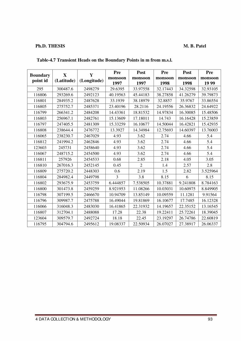
4.18 Boundary Conditions
The boundary is located along the catchment boundary of the Mahi Basin. The boundary of
the study area is divided into number of segments. Twenty four points are selected on the
perimeter of the study area as shown in figure 4.17. Heads on these points are obtained using
available reduced water level of wells for pre monsoon and post monsoon periods of years
1997, 1998, 1999, 2003, 2004, 2005, 2006 and 2007.The Iso-RWL contour maps are
prepared using surfer 6.0 Software and head at boundary points are interpolated or
extrapolated. The heads on the South-West and North-East boundary of the study area are
estimated using the RL’s of Mahi River water levels at Khanpur and at Dhuvaran
respectively. The flow domain is bounded by head-dependent flow (Transient head)
boundary conditions. The transient heads on the boundary points are presented in table 4.7.
Figure 4.17 Location of Boundary points on the Study Area
Ph.D. THESIS M. B. Patel
4 DATA COLLECTION & METHODOLOGY 93
Table-4.7 Transient Heads on the Boundary Points in m from m.s.l.
Boundary
point id
X
(Latitude)
Y
(Longitude)
Pre
monsoon
1997
Post
monsoon
1997
Pre
monsoon
1998
Post
monsoon
1998
Pre
monsoon
19 99
295 300487.6 2498279 29.6395 33.97558 32.17443 34.32598 32.93105
116806 293269.6 2492123 40.19563 45.44183 38.27858 41.26279 39.79873
116801 284935.2 2487628 33.1939 38.18979 32.8857 35.9767 33.86554
116805 275752.7 2485371 23.40196 28.2116 24.19556 26.36832 24.64922
116799 266341.2 2484208 14.43361 18.81532 14.97834 16.30085 15.48506
116803 256967.1 2482761 15.13609 17.18011 14.743 16.16428 15.23859
116797 247405.5 2481309 15.33259 16.10677 14.50044 16.42821 15.42935
116808 238644.4 2476772 13.3927 14.34984 12.75693 14.60397 13.76003
116065 238230.7 2467029 4.93 3.62 2.74 4.66 5.4
116812 241994.2 2462846 4.93 3.62 2.74 4.66 5.4
123603 245731 2458640 4.93 3.62 2.74 4.66 5.4
116067 248715.2 2454500 4.93 3.62 2.74 4.66 5.4
116811 257926 2454533 0.68 2.85 2.18 4.05 3.05
116810 267016.3 2452145 0.45 2 1.4 2.57 2.8
116809 275720.2 2448303 0.6 2.19 1.5 2.82 3.525964
116804 284982.4 2449798 3 3.8 8.15 6 8.15
116802 293675.9 2453759 6.444857 7.538505 10.37881 9.241808 8.784163
116800 301473.8 2459259 8.921953 11.08266 10.03031 10.60975 8.849905
116798 307199.5 2466670 10.94709 13.85149 10.09559 11.1281 9.91564
116796 309987.7 2475788 16.49044 19.81869 16.10677 17.7485 16.12328
116066 316048.3 2483030 16.41865 22.31932 14.19657 22.35152 13.16545
116807 312704.1 2488088 17.28 22.38 19.22411 25.72261 18.39045
123604 309579.7 2492724 18.18 22.45 23.19297 26.74786 22.60819
116795 304794.6 2495612 19.08337 22.50934 26.07027 27.38917 26.06337
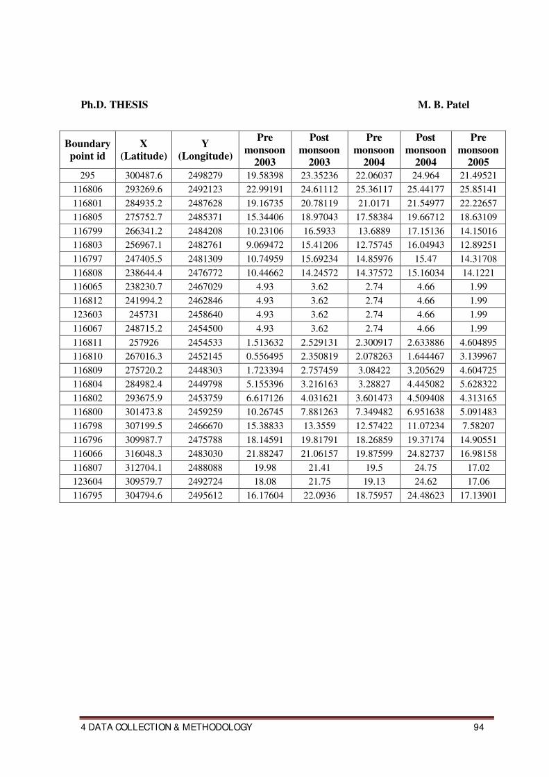
Ph.D. THESIS M. B. Patel
4 DATA COLLECTION & METHODOLOGY 94
Boundary
point id
X
(Latitude)
Y
(Longitude)
Pre
monsoon
2003
Post
monsoon
2003
Pre
monsoon
2004
Post
monsoon
2004
Pre
monsoon
2005
295 300487.6 2498279 19.58398 23.35236 22.06037 24.964 21.49521
116806 293269.6 2492123 22.99191 24.61112 25.36117 25.44177 25.85141
116801 284935.2 2487628 19.16735 20.78119 21.0171 21.54977 22.22657
116805 275752.7 2485371 15.34406 18.97043 17.58384 19.66712 18.63109
116799 266341.2 2484208 10.23106 16.5933 13.6889 17.15136 14.15016
116803 256967.1 2482761 9.069472 15.41206 12.75745 16.04943 12.89251
116797 247405.5 2481309 10.74959 15.69234 14.85976 15.47 14.31708
116808 238644.4 2476772 10.44662 14.24572 14.37572 15.16034 14.1221
116065 238230.7 2467029 4.93 3.62 2.74 4.66 1.99
116812 241994.2 2462846 4.93 3.62 2.74 4.66 1.99
123603 245731 2458640 4.93 3.62 2.74 4.66 1.99
116067 248715.2 2454500 4.93 3.62 2.74 4.66 1.99
116811 257926 2454533 1.513632 2.529131 2.300917 2.633886 4.604895
116810 267016.3 2452145 0.556495 2.350819 2.078263 1.644467 3.139967
116809 275720.2 2448303 1.723394 2.757459 3.08422 3.205629 4.604725
116804 284982.4 2449798 5.155396 3.216163 3.28827 4.445082 5.628322
116802 293675.9 2453759 6.617126 4.031621 3.601473 4.509408 4.313165
116800 301473.8 2459259 10.26745 7.881263 7.349482 6.951638 5.091483
116798 307199.5 2466670 15.38833 13.3559 12.57422 11.07234 7.58207
116796 309987.7 2475788 18.14591 19.81791 18.26859 19.37174 14.90551
116066 316048.3 2483030 21.88247 21.06157 19.87599 24.82737 16.98158
116807 312704.1 2488088 19.98 21.41 19.5 24.75 17.02
123604 309579.7 2492724 18.08 21.75 19.13 24.62 17.06
116795 304794.6 2495612 16.17604 22.0936 18.75957 24.48623 17.13901
Ph.D. THESIS M. B. Patel
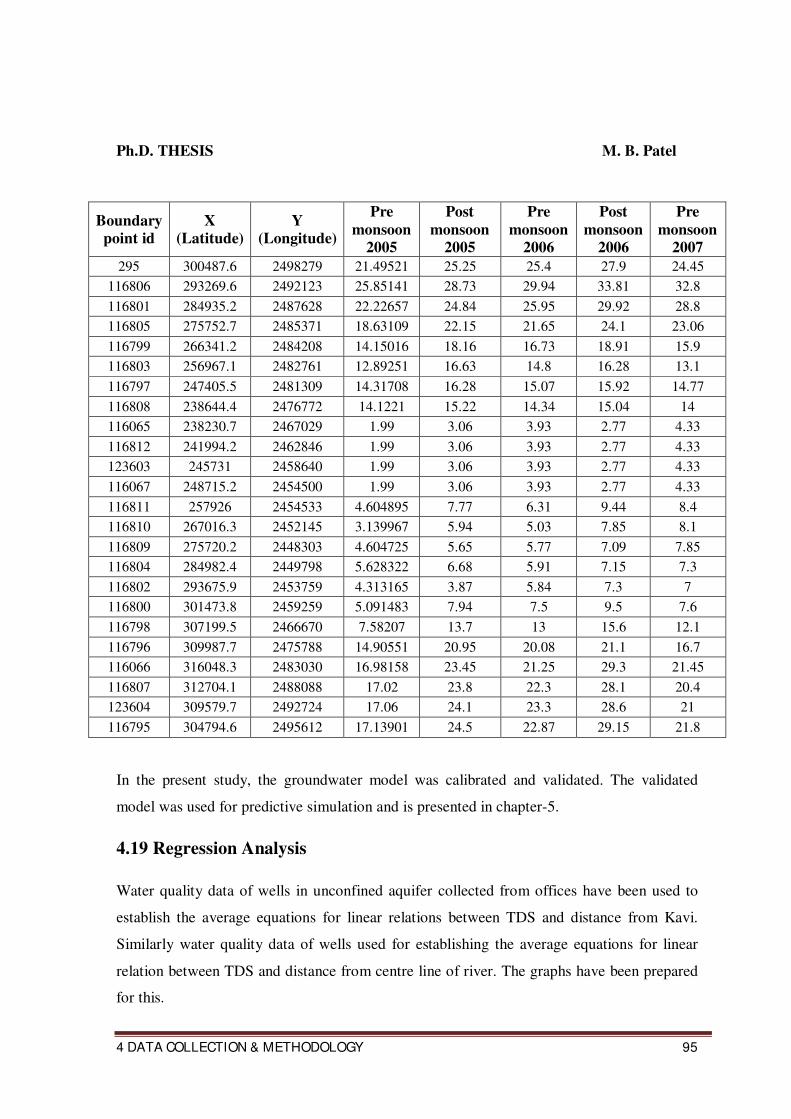
4 DATA COLLECTION & METHODOLOGY 95
In the present study, the groundwater model was calibrated and validated. The validated
model was used for predictive simulation and is presented in chapter-5.
4.19 Regression Analysis
Water quality data of wells in unconfined aquifer collected from offices have been used to
establish the average equations for linear relations between TDS and distance from Kavi.
Similarly water quality data of wells used for establishing the average equations for linear
relation between TDS and distance from centre line of river. The graphs have been prepared
for this.
Boundary
point id
X
(Latitude)
Y
(Longitude)
Pre
monsoon
2005
Post
monsoon
2005
Pre
monsoon
2006
Post
monsoon
2006
Pre
monsoon
2007
295 300487.6 2498279 21.49521 25.25 25.4 27.9 24.45
116806 293269.6 2492123 25.85141 28.73 29.94 33.81 32.8
116801 284935.2 2487628 22.22657 24.84 25.95 29.92 28.8
116805 275752.7 2485371 18.63109 22.15 21.65 24.1 23.06
116799 266341.2 2484208 14.15016 18.16 16.73 18.91 15.9
116803 256967.1 2482761 12.89251 16.63 14.8 16.28 13.1
116797 247405.5 2481309 14.31708 16.28 15.07 15.92 14.77
116808 238644.4 2476772 14.1221 15.22 14.34 15.04 14
116065 238230.7 2467029 1.99 3.06 3.93 2.77 4.33
116812 241994.2 2462846 1.99 3.06 3.93 2.77 4.33
123603 245731 2458640 1.99 3.06 3.93 2.77 4.33
116067 248715.2 2454500 1.99 3.06 3.93 2.77 4.33
116811 257926 2454533 4.604895 7.77 6.31 9.44 8.4
116810 267016.3 2452145 3.139967 5.94 5.03 7.85 8.1
116809 275720.2 2448303 4.604725 5.65 5.77 7.09 7.85
116804 284982.4 2449798 5.628322 6.68 5.91 7.15 7.3
116802 293675.9 2453759 4.313165 3.87 5.84 7.3 7
116800 301473.8 2459259 5.091483 7.94 7.5 9.5 7.6
116798 307199.5 2466670 7.58207 13.7 13 15.6 12.1
116796 309987.7 2475788 14.90551 20.95 20.08 21.1 16.7
116066 316048.3 2483030 16.98158 23.45 21.25 29.3 21.45
116807 312704.1 2488088 17.02 23.8 22.3 28.1 20.4
123604 309579.7 2492724 17.06 24.1 23.3 28.6 21
116795 304794.6 2495612 17.13901 24.5 22.87 29.15 21.8
Ph.D. THESIS M. B. Patel
4 DATA COLLECTION & METHODOLOGY 96
The Multiple Linear Regression Analysis has been carried out for establishing the linear
relationships between three parameters such as TDS, Distance from Kavi and RWL. TDS has
been taken as dependent variable because the analysis has been carried out to study the
variation of salinity in Mahi estuarine area and other two have been taken as independent
variables.
The effect of recharge due to Mahi Right Bank Canal (MRBC) irrigation have been observed
in the area on right bank of the river, while in the area on the left bank of the river, the
recharge due to irrigation is not observed as there is no left bank irrigation canal in past. So,
the analysis for left bank, right bank and for both bank have been carried out separately.
Similarly the Multiple Linear Regression Analysis has been carried out for establishing the
linear relationships between four parameters such as TDS, Distances from Kavi and RWL
and rainfall.
4.19.1 Year Wise Variation in TDS With Reference to Rainfall and Lab Analysis for
Water Quality
Another analysis which shows the year wise variation in TDS with reference to Rainfall for
different wells in Anand, Borsad, Khambhat (Cambay), Savli, Vadodara and Padra talukas
have been done.
Water samples of 36 wells parallel to Mahi river in May and Nov. 2003 collected and tested
for important parameters like EC, PH, TDS, Ca, Mg, Na, CO3,HCO3, Cl,SO4, K and TH
The results are graphically represented as TDS, Cl and TH v/s distances from Kavi and
distances from centre line of river.
Related Documents