Visualization, Summer Term 03 VIS, University of Stuttgart 1 4. Basic Mapping Techniques • Mapping from (filtered) data to renderable representation • Most important part of visualization • Possible visual representations: • Position • Size • Orientation • Shape • Brightness • Color (hue, saturation) • …. Visualization, Summer Term 03 VIS, University of Stuttgart 2 4. Basic Mapping Techniques • Efficiency and effectiveness depends on input data: • Nominal • Ordinal • Quantitative • Psychological investigations to evaluate the appropriateness of mapping approaches

Welcome message from author
This document is posted to help you gain knowledge. Please leave a comment to let me know what you think about it! Share it to your friends and learn new things together.
Transcript
Visualization, Summer Term 2002 11.06.2003
1
Visualization, Summer Term 03 VIS, University of Stuttgart1
4. Basic Mapping Techniques
• Mapping from (filtered) data to renderable representation• Most important part of visualization• Possible visual representations:
• Position• Size• Orientation• Shape• Brightness• Color (hue, saturation)• ….
Visualization, Summer Term 03 VIS, University of Stuttgart2
4. Basic Mapping Techniques
• Efficiency and effectiveness depends on input data:• Nominal• Ordinal• Quantitative
• Psychological investigations to evaluate the appropriateness of mapping approaches
Visualization, Summer Term 2002 11.06.2003
2
Visualization, Summer Term 03 VIS, University of Stuttgart3
4.1. Diagram Techniques
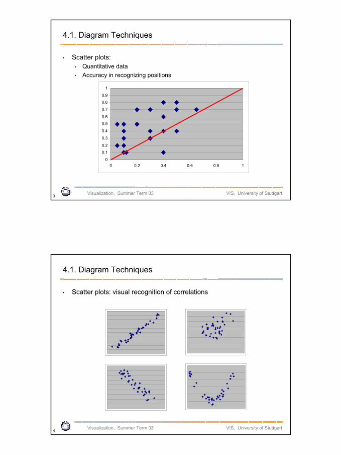
• Scatter plots:• Quantitative data• Accuracy in recognizing positions
0
0.1
0.2
0.3
0.4
0.5
0.6
0.7
0.8
0.9
1
0 0.2 0.4 0.6 0.8 1
Visualization, Summer Term 03 VIS, University of Stuttgart4
4.1. Diagram Techniques
• Scatter plots: visual recognition of correlations
Visualization, Summer Term 2002 11.06.2003
3
Visualization, Summer Term 03 VIS, University of Stuttgart5
4.1. Diagram Techniques
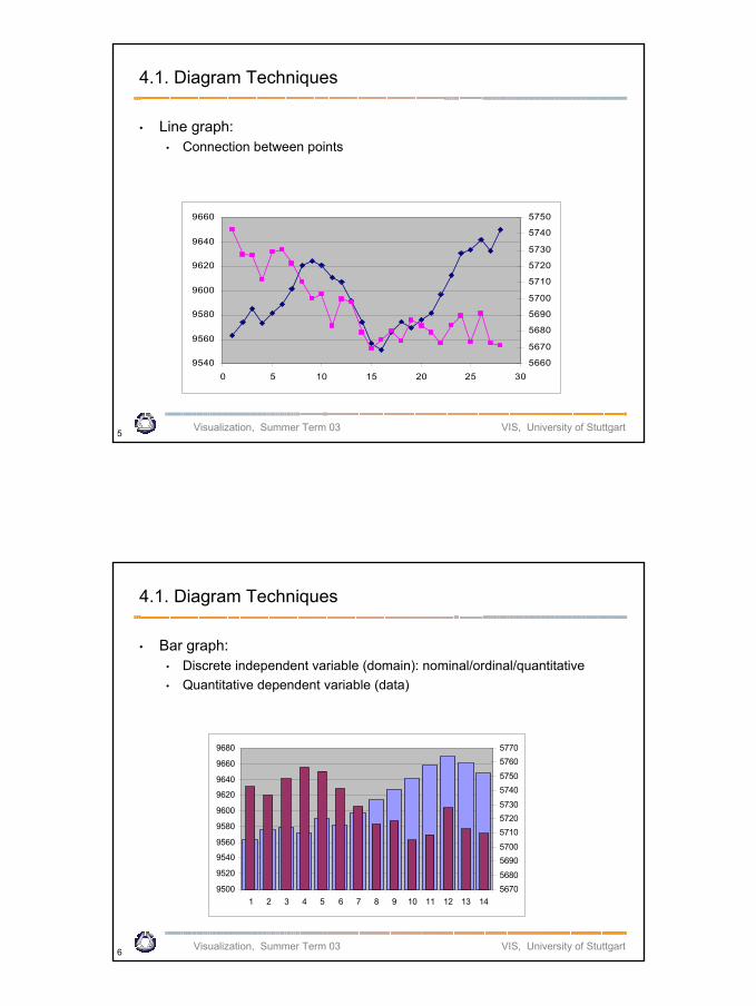
• Line graph:• Connection between points
9540
9560
9580
9600
9620
9640
9660
0 5 10 15 20 25 305660
5670
5680
5690
5700
5710
5720
5730
5740
5750
Visualization, Summer Term 03 VIS, University of Stuttgart6
4.1. Diagram Techniques
• Bar graph:• Discrete independent variable (domain): nominal/ordinal/quantitative• Quantitative dependent variable (data)
9500
9520
9540
9560
9580
9600
9620
9640
9660
9680
1 2 3 4 5 6 7 8 9 10 11 12 13 1456705680
56905700
571057205730
57405750
57605770
Visualization, Summer Term 2002 11.06.2003
4
Visualization, Summer Term 03 VIS, University of Stuttgart7
4.1. Diagram Techniques
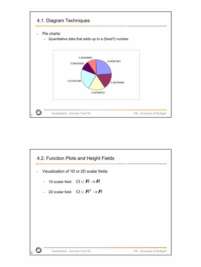
• Pie charts:• Quantitative data that adds up to a (fixed?) number
0.645901961
0.450794846
0.467508703
0.614301398
0.265353929
0.252258892
Visualization, Summer Term 03 VIS, University of Stuttgart8
4.2. Function Plots and Height Fields
• Visualization of 1D or 2D scalar fields
• 1D scalar field:
• 2D scalar field:
RIRI →⊂Ω
RIRI →⊂Ω 2
Visualization, Summer Term 2002 11.06.2003
5
Visualization, Summer Term 03 VIS, University of Stuttgart9
4.2. Function Plots and Height Fields
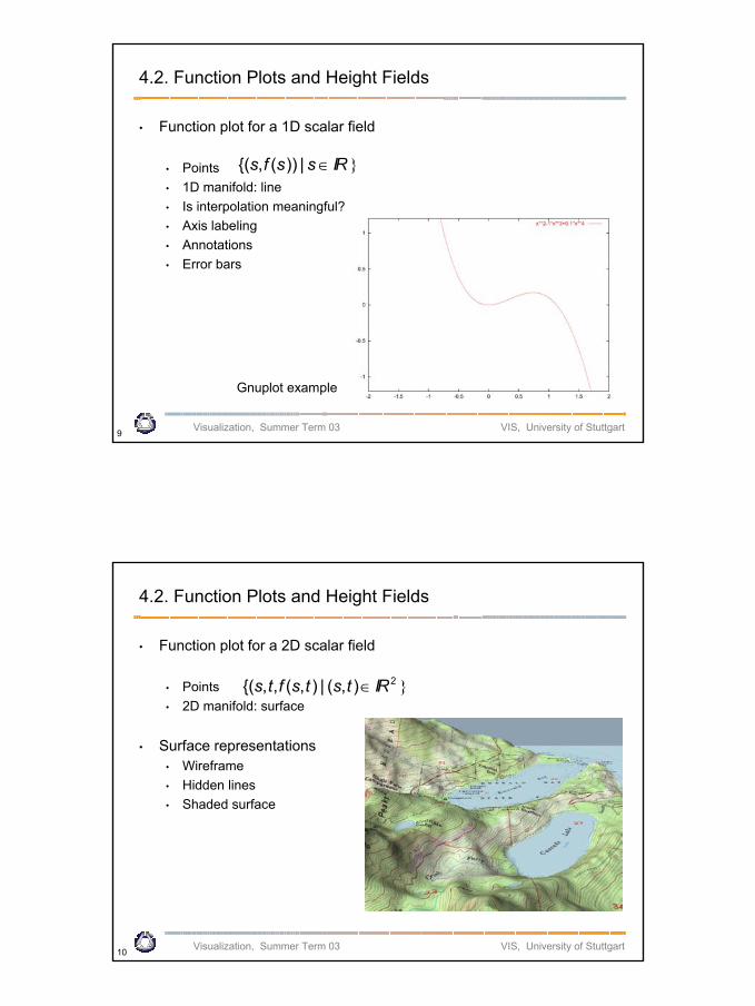
• Function plot for a 1D scalar field
• Points• 1D manifold: line• Is interpolation meaningful?• Axis labeling• Annotations• Error bars
RIssfs ∈|))(,(
Gnuplot example
Visualization, Summer Term 03 VIS, University of Stuttgart10
4.2. Function Plots and Height Fields
• Function plot for a 2D scalar field
• Points• 2D manifold: surface
• Surface representations• Wireframe• Hidden lines• Shaded surface
2),(|),(,,( RItstsfts ∈
Visualization, Summer Term 2002 11.06.2003
6
Visualization, Summer Term 03 VIS, University of Stuttgart11
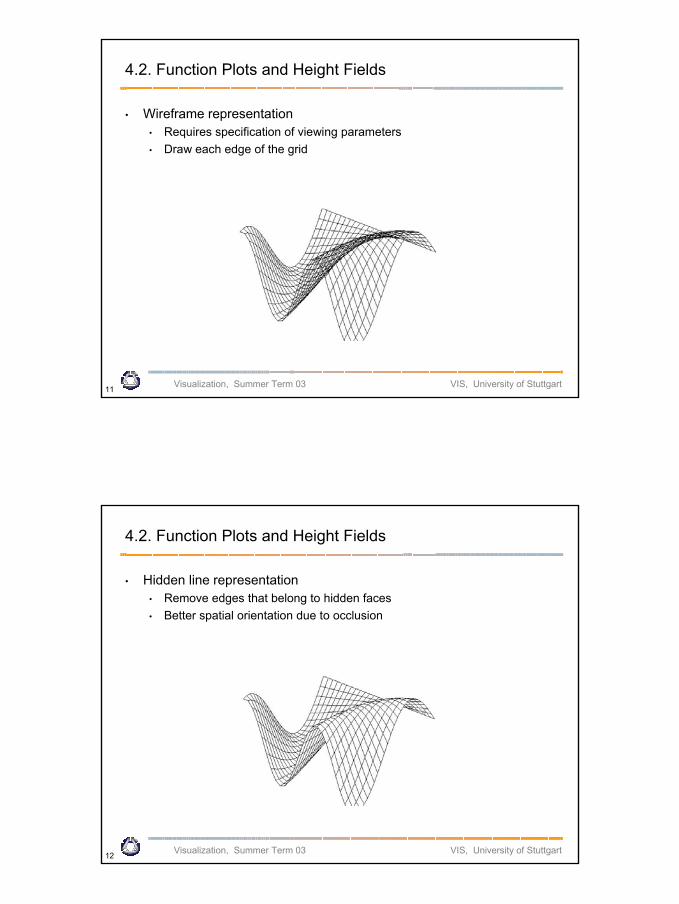
4.2. Function Plots and Height Fields
• Wireframe representation• Requires specification of viewing parameters• Draw each edge of the grid
Visualization, Summer Term 03 VIS, University of Stuttgart12
4.2. Function Plots and Height Fields
• Hidden line representation• Remove edges that belong to hidden faces• Better spatial orientation due to occlusion
Visualization, Summer Term 2002 11.06.2003
7
Visualization, Summer Term 03 VIS, University of Stuttgart13
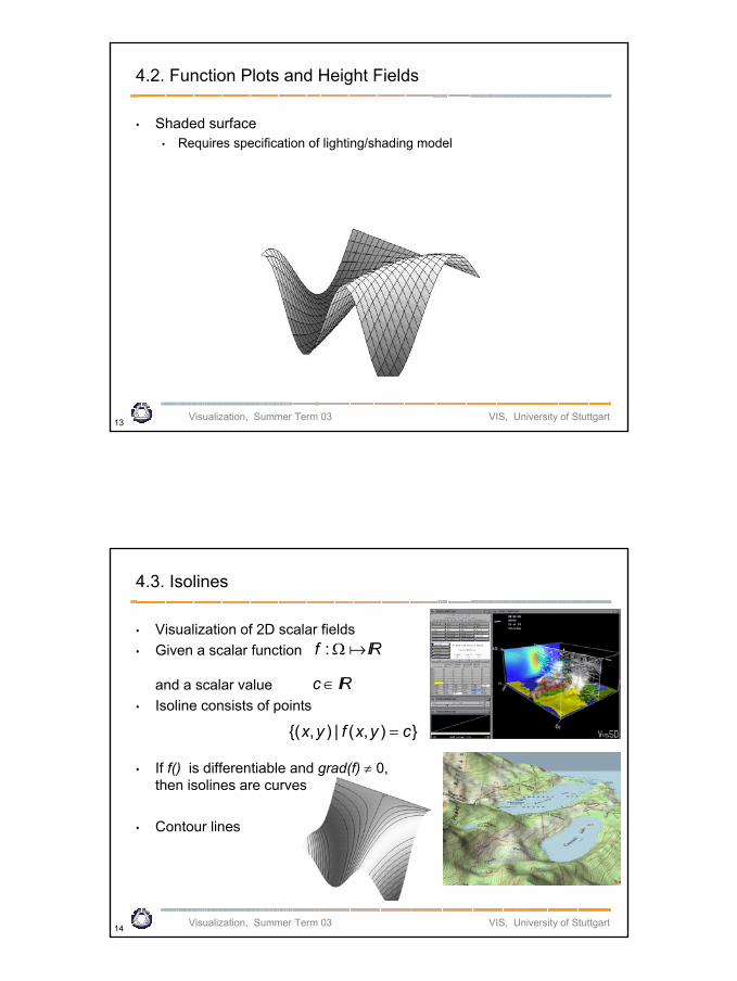
4.2. Function Plots and Height Fields
• Shaded surface• Requires specification of lighting/shading model
Visualization, Summer Term 03 VIS, University of Stuttgart14
4.3. Isolines
• Visualization of 2D scalar fields• Given a scalar function
and a scalar value • Isoline consists of points
• If f() is differentiable and grad(f) ≠ 0, then isolines are curves
• Contour lines
RIf aΩ:
RIc∈
),(|),( cyxfyx =
Visualization, Summer Term 2002 11.06.2003
8
Visualization, Summer Term 03 VIS, University of Stuttgart15
4.3. Isolines
Visualization, Summer Term 03 VIS, University of Stuttgart16
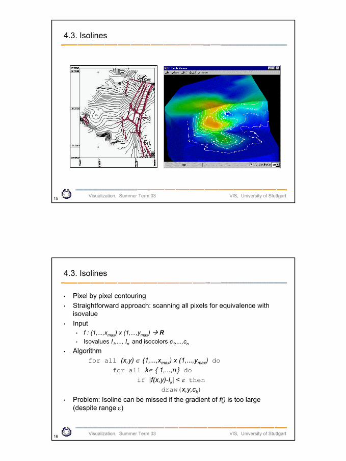
4.3. Isolines
• Pixel by pixel contouring• Straightforward approach: scanning all pixels for equivalence with
isovalue• Input
• f : (1,...,xmax) x (1,...,ymax) R• Isovalues I1,..., In and isocolors c1,...,cn
• Algorithmfor all (x,y) ∈ (1,...,xmax) x (1,...,ymax) do
for all k∈ 1,...,n doif |f(x,y)-Ik| < ε then
draw(x,y,ck)• Problem: Isoline can be missed if the gradient of f() is too large
(despite range ε)
Visualization, Summer Term 2002 11.06.2003
9
Visualization, Summer Term 03 VIS, University of Stuttgart17
4.3. Isolines
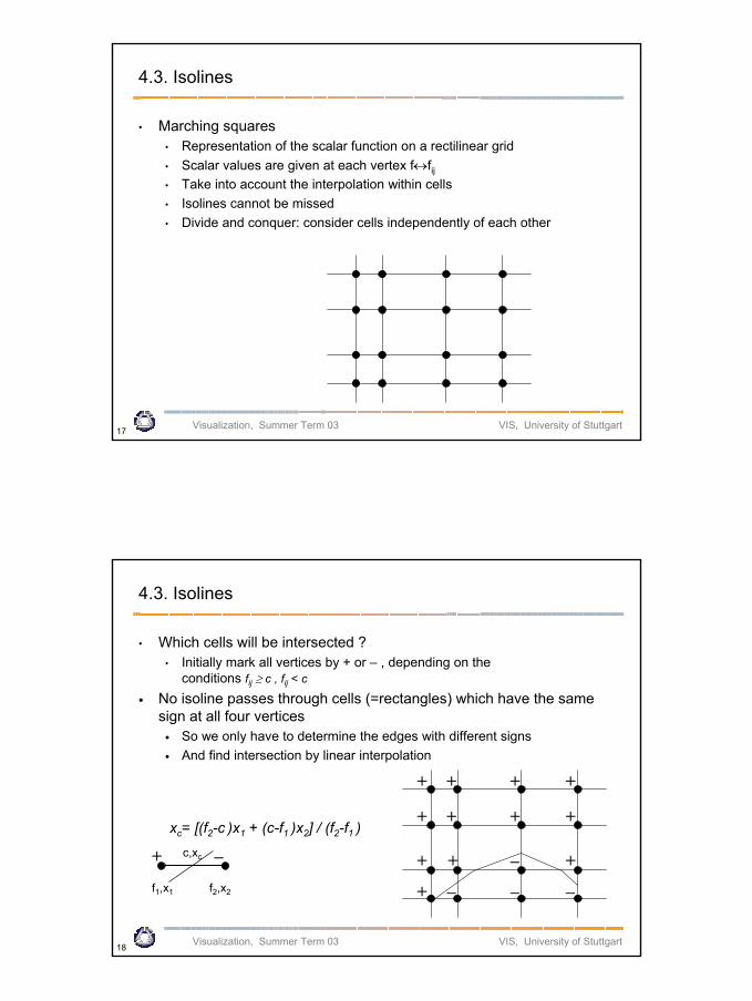
• Marching squares• Representation of the scalar function on a rectilinear grid• Scalar values are given at each vertex f↔fij• Take into account the interpolation within cells• Isolines cannot be missed• Divide and conquer: consider cells independently of each other
Visualization, Summer Term 03 VIS, University of Stuttgart18
4.3. Isolines
• Which cells will be intersected ?• Initially mark all vertices by + or – , depending on the
conditions fij ≥ c , fij < c
• No isoline passes through cells (=rectangles) which have the same sign at all four vertices • So we only have to determine the edges with different signs• And find intersection by linear interpolation
+ + + +
+ + + +
+ + +
+
–
–––
+ –
f1,x1 f2,x2
c,xc
xc= [(f2-c )x1 + (c-f1 )x2] / (f2-f1 )
Visualization, Summer Term 2002 11.06.2003
10
Visualization, Summer Term 03 VIS, University of Stuttgart19
4.3. Isolines
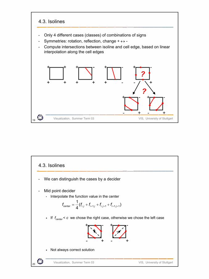
• Only 4 different cases (classes) of combinations of signs• Symmetries: rotation, reflection, change + ↔ -• Compute intersections between isoline and cell edge, based on linear
interpolation along the cell edges
+ +
+ +
+ -
+ +
+ -
+ -
+ -
- +?
+ -
- +
+ -
- +
?
Visualization, Summer Term 03 VIS, University of Stuttgart20
4.3. Isolines
• We can distinguish the cases by a decider
• Mid point decider• Interpolate the function value in the center
• If fcenter < c we chose the right case, otherwise we chose the left case
• Not always correct solution
+ -
- +
++ -
- +
-
)(41
1,11,,1,center ++++ +++= jijijiji fffff
Visualization, Summer Term 2002 11.06.2003
11
Visualization, Summer Term 03 VIS, University of Stuttgart21
4.3. Isolines
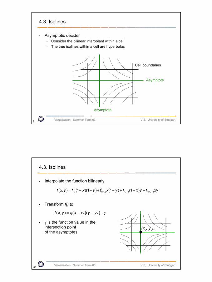
• Asymptotic decider• Consider the bilinear interpolant within a cell• The true isolines within a cell are hyperbolas
Asymptote
Cell boundaries
Asymptote
Visualization, Summer Term 03 VIS, University of Stuttgart22
4.3. Isolines
• Interpolate the function bilinearly
• Transform f() to
• γ is the function value in the intersection point of the asymptotes
xyfyxfyxfyxfyxf jijijiji 111,,1, )1()1()1)(1(),( ++++ +−+−+−−=
γη +−−= ))((),( 00 yyxxyxf
(x0, y0)
Visualization, Summer Term 2002 11.06.2003
12
Visualization, Summer Term 03 VIS, University of Stuttgart23
4.3. Isolines
• If γ ≤ c we chose the right case, otherwise we chose the left one
+
+ -
- +
-
+ -
- +
Visualization, Summer Term 03 VIS, University of Stuttgart24
4.3. Isolines
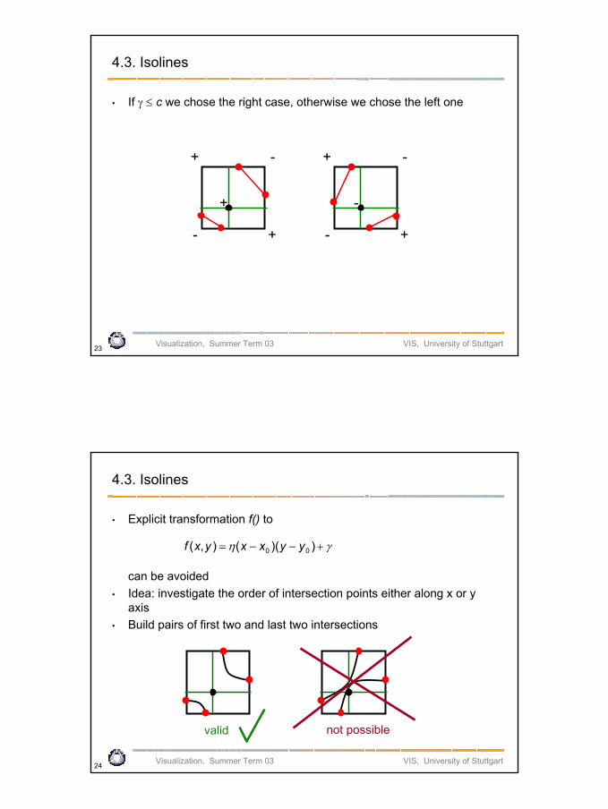
• Explicit transformation f() to
can be avoided• Idea: investigate the order of intersection points either along x or y
axis• Build pairs of first two and last two intersections
γη +−−= ))((),( 00 yyxxyxf
valid not possible
Visualization, Summer Term 2002 11.06.2003
13
Visualization, Summer Term 03 VIS, University of Stuttgart25
4.3. Isolines
• Cell order approach for marching squares• Traverse all cells of the grid• Apply marching squares technique to each single cell
• Disadvantage of cell order method• Every vertex (of the isoline) and every edge in the grid is processed twice• The output is just a collection of pieces of isolines which have to be post-
processed to get (closed) polylines
Visualization, Summer Term 03 VIS, University of Stuttgart26
4.3. Isolines
• Contour tracing approach• Start at a seed point of the isoline• Move to the neighboring cell into which the isoline enters• Trace isoline until
• Bounds of the domain are reached or• Isoline is closed
• Problem: How to find seed points efficiently?• In a preprocessing step, mark all cells which have a sign change• Remove marker from cells which are traversed during contour tracing
(unless there are 4 intersection edges! )
Visualization, Summer Term 2002 11.06.2003
14
Visualization, Summer Term 03 VIS, University of Stuttgart27
4.3. Isolines
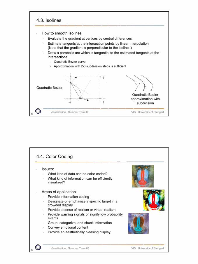
• How to smooth isolines• Evaluate the gradient at vertices by central differences• Estimate tangents at the intersection points by linear interpolation
(Note that the gradient is perpendicular to the isoline !)• Draw a parabolic arc which is tangential to the estimated tangents at the
intersections • Quadratic Bezier curve• Approximation with 2-3 subdivision steps is sufficient
•
•
+ +
+–
Quadratic Bezier
Quadratic Bezierapproximation with
subdivision
Visualization, Summer Term 03 VIS, University of Stuttgart28
4.4. Color Coding
• Issues:• What kind of data can be color-coded?• What kind of information can be efficiently
visualized?
• Areas of application• Provide information coding• Designate or emphasize a specific target in a
crowded display • Provide a sense of realism or virtual realism • Provide warning signals or signify low probability
events• Group, categorize, and chunk information• Convey emotional content • Provide an aesthetically pleasing display
Visualization, Summer Term 2002 11.06.2003
15
Visualization, Summer Term 03 VIS, University of Stuttgart29
4.4. Color Coding
• Possible problems:• Distract the user when inadequately used • Dependent on viewing and stimulus conditions • Ineffective for color deficient individuals (use redundancy)• Results in information overload • Unintentionally conflict with cultural conventions • Cause unintended visual effects and discomfort
Visualization, Summer Term 03 VIS, University of Stuttgart30
4.4. Color Coding
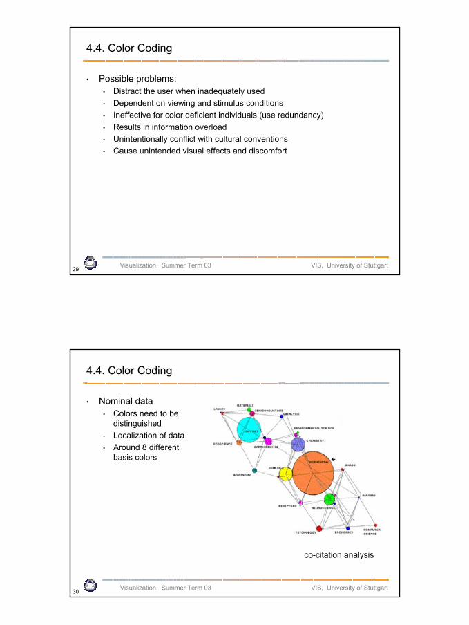
• Nominal data• Colors need to be
distinguished• Localization of data• Around 8 different
basis colors
co-citation analysis

Visualization, Summer Term 2002 11.06.2003
16
Visualization, Summer Term 03 VIS, University of Stuttgart31
4.4. Color Coding
• Nominal data
Visualization, Summer Term 03 VIS, University of Stuttgart32
4.4. Color Coding
• Ordinal and quantitative data• Ordering of data should be represented by ordering of colors• Psychological aspects• x1 < x2 < ... < xn E(c1) < E(c2 ) < ... < E(cn )
• Color coding for scalar data• Assign to each scalar value a different color value • Assignment via transfer function T
T : scalarvalue → colorvalue • Code color values into a color lookup table
0Scalar ∈(0,1)
RiGiBi
(0,1) → (0,N-1) 255
Visualization, Summer Term 2002 11.06.2003
17
Visualization, Summer Term 03 VIS, University of Stuttgart33
4.4. Color Coding
• Pre-shading vs. post-shading• Pre-shading
• Assign color values to original function values (e.g. at vertices of a cell)• Interpolate between color values (within a cell)
• Post-shading• Interpolate between scalar values (within a cell)• Assign color values to interpolated scalar values
• Linear transfer function for color coding• Specify color for fmin and for fmax
• (Rmin ,Gmin , Bmin) and (Rmax , Gmax , Bmax)• Linearly interpolate between them
)()( maxmaxmaxminmax
maxminminmin
minmax
min ,B,GRffff,B,GR
fffff
−−
+−−
a
Visualization, Summer Term 03 VIS, University of Stuttgart34
4.4. Color Coding
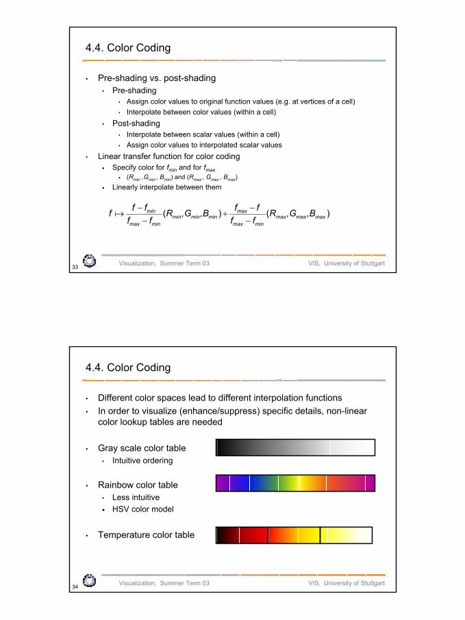
• Different color spaces lead to different interpolation functions• In order to visualize (enhance/suppress) specific details, non-linear
color lookup tables are needed
• Gray scale color table• Intuitive ordering
• Rainbow color table• Less intuitive• HSV color model
• Temperature color table
Visualization, Summer Term 2002 11.06.2003
18
Visualization, Summer Term 03 VIS, University of Stuttgart35
4.4. Color Coding
• Bivariate and trivariate color tables are not very useful:• No intuitive ordering• Colors hard to distinguish
• Many more color tables for specific applications• Design of good color tables depends on psychological / perceptional
issues
• Often interactive specification of transfer functions to extract important features
Visualization, Summer Term 03 VIS, University of Stuttgart36
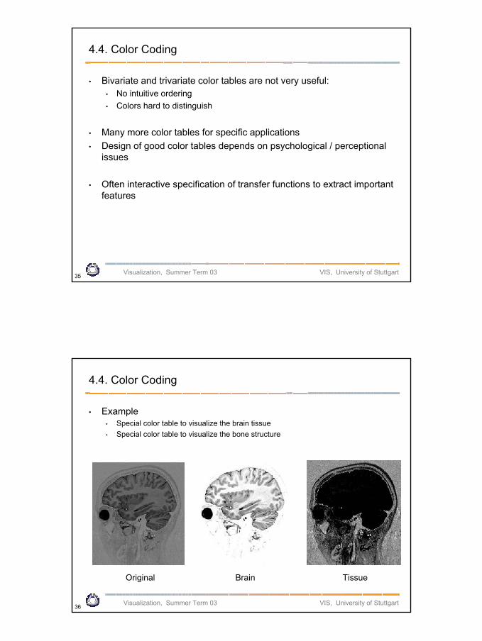
4.4. Color Coding
• Example• Special color table to visualize the brain tissue• Special color table to visualize the bone structure
Original Brain Tissue
Visualization, Summer Term 2002 11.06.2003
19
Visualization, Summer Term 03 VIS, University of Stuttgart37
4.5. Glyphs and Icons
• Glyphs and icons• Features should be easy to distinguish and combine• Icons should be separated from each other• Mainly used for multivariate data
Visualization, Summer Term 03 VIS, University of Stuttgart38
4.5. Glyphs and Icons
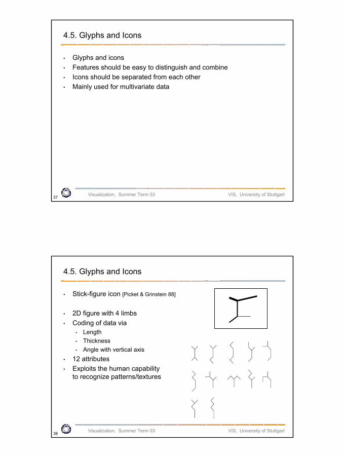
• Stick-figure icon [Picket & Grinstein 88]
• 2D figure with 4 limbs• Coding of data via
• Length• Thickness• Angle with vertical axis
• 12 attributes• Exploits the human capability
to recognize patterns/textures

Visualization, Summer Term 2002 11.06.2003
20
Visualization, Summer Term 03 VIS, University of Stuttgart39
4.5. Glyphs and Icons
• Stick-figure icon
Visualization, Summer Term 03 VIS, University of Stuttgart40
4.5. Glyphs and Icons
• Color icons [Levkowitz 91]
• Subdivision of a basic figure(triangle, square, …)into edges and faces
• Mapping of data to faces viacolor tables
• Grouping by emphasizing edgesor faces
Visualization, Summer Term 2002 11.06.2003
21
Visualization, Summer Term 03 VIS, University of Stuttgart41
4.5. Glyphs and Icons
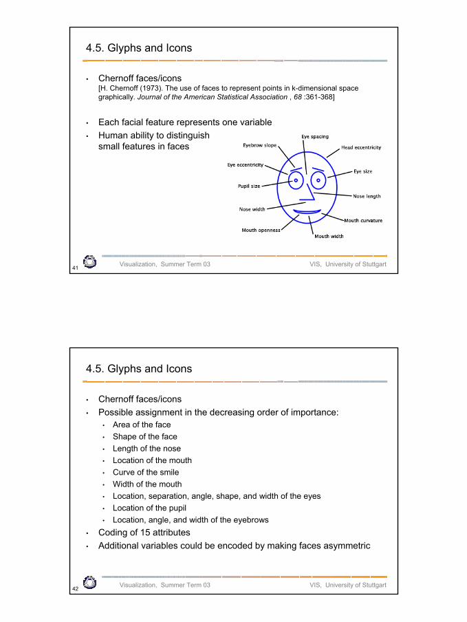
• Chernoff faces/icons [H. Chernoff (1973). The use of faces to represent points in k-dimensional space graphically. Journal of the American Statistical Association , 68 :361-368]
• Each facial feature represents one variable• Human ability to distinguish
small features in faces
Visualization, Summer Term 03 VIS, University of Stuttgart42
4.5. Glyphs and Icons
• Chernoff faces/icons• Possible assignment in the decreasing order of importance:
• Area of the face • Shape of the face • Length of the nose • Location of the mouth • Curve of the smile • Width of the mouth • Location, separation, angle, shape, and width of the eyes • Location of the pupil • Location, angle, and width of the eyebrows
• Coding of 15 attributes • Additional variables could be encoded by making faces asymmetric
Visualization, Summer Term 2002 11.06.2003
22
Visualization, Summer Term 03 VIS, University of Stuttgart43
4.5. Glyphs and Icons
• Chernoff faces/icons
Visualization, Summer Term 03 VIS, University of Stuttgart44
4.5. Glyphs and Icons
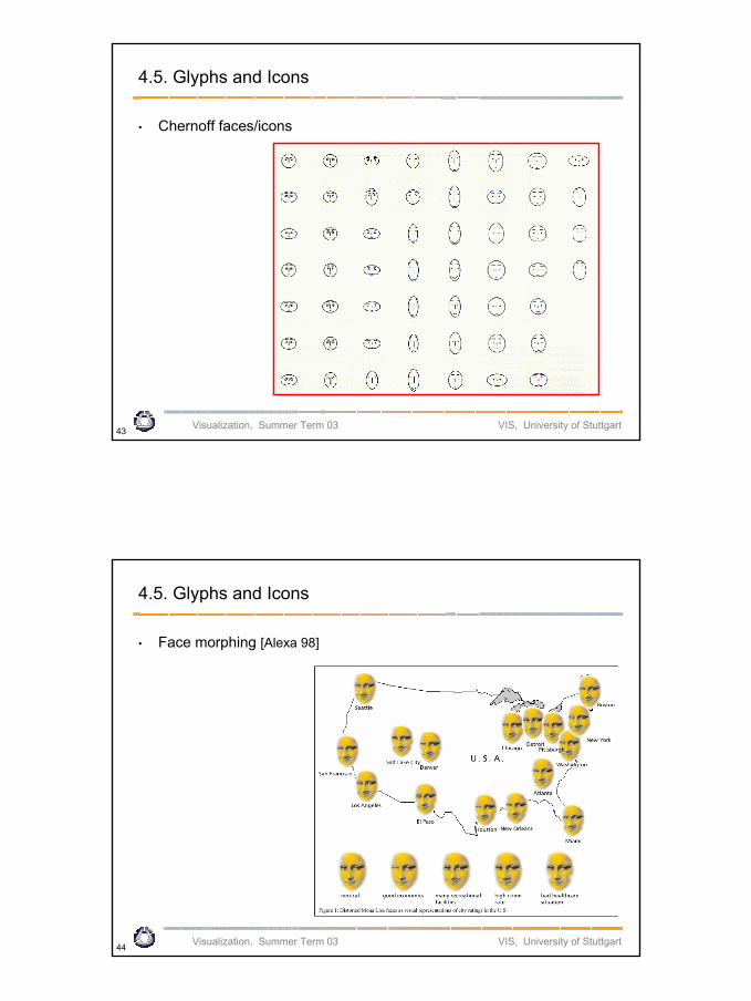
• Face morphing [Alexa 98]

Visualization, Summer Term 2002 11.06.2003
23
Visualization, Summer Term 03 VIS, University of Stuttgart45
4.5. Glyphs and Icons
• Circular icon plots:• Star plots• Sun ray plots• etc…
• Follow a "spoked wheel" format• Values of variables are represented by distances between the center
("hub") of the icon and its edges
Visualization, Summer Term 03 VIS, University of Stuttgart46
4.5. Glyphs and Icons
• Star glyphs [S. E. Fienberg: Graphical methods in statistics. The American Statistician, 33:165-178, 1979]
• A star is composed of equally spaced radii, stemming from the center• The length of the spike is proportional to the value of the respective
attribute • The first spike/attribute
is to the right• Subsequent spikes
are counter-clockwise • The ends of the rays
are connected by a line
Visualization, Summer Term 2002 11.06.2003
24
Visualization, Summer Term 03 VIS, University of Stuttgart47
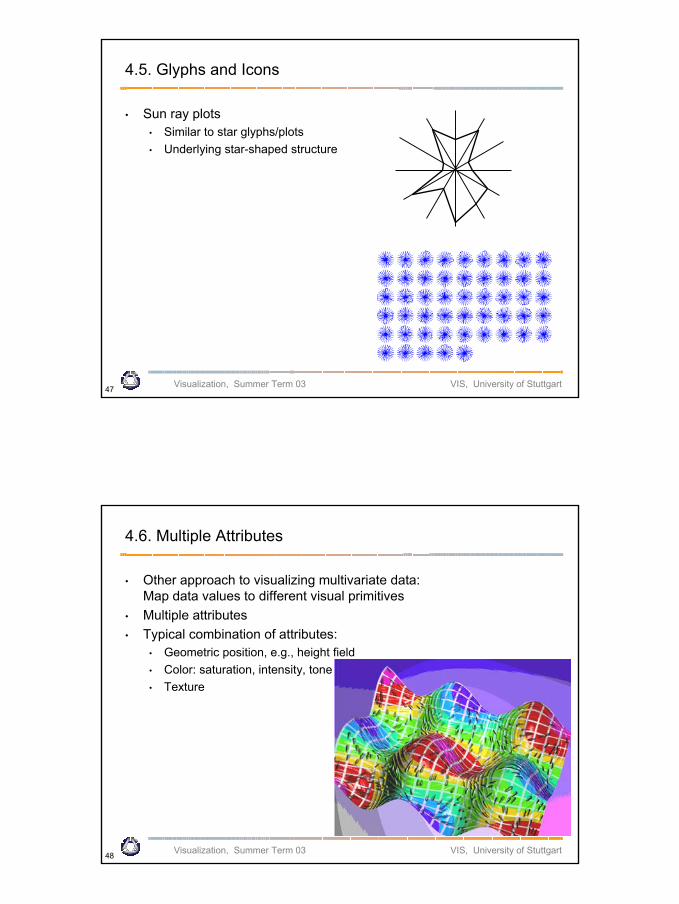
4.5. Glyphs and Icons
• Sun ray plots• Similar to star glyphs/plots• Underlying star-shaped structure
Visualization, Summer Term 03 VIS, University of Stuttgart48
4.6. Multiple Attributes
• Other approach to visualizing multivariate data:Map data values to different visual primitives
• Multiple attributes• Typical combination of attributes:
• Geometric position, e.g., height field• Color: saturation, intensity, tone • Texture
Related Documents


