4-5 The Poisson Distribution

Chapter 5, Triola, Elementary Statistics, MATH 1342

Slide 1Chapter 5

Normal Probability Distributions

5-1 Overview5-2 The Standard Normal Distribution5-3 Applications of Normal Distributions5-4 Sampling Distributions and Estimators5-5 The Central Limit Theorem5-6 Normal as Approximation to Binomial5-7 Determining Normality


Slide 2

Created by Erin Hodgess, Houston, Texas

Section 5-1 Overview


Slide 3

Continuous random variableNormal distribution

Overview

Figure 5-1 (p.226)

Formula 5-1

f(x) = σ 2 π

x-μσ )2(

e-12


Slide 4

Section 5-2 The Standard Normal

Distribution


Slide 5

Uniform Distribution is a probability distribution in which the continuous random variable values are spread evenly over the range of possibilities; the graph results in a rectangular shape.

Definitions


Slide 6

Density Curve (or probability density function is the graph of a continuous probability distribution.

Definitions (p.228)

1. The total area under the curve must equal 1.

2. Every point on the curve must have a vertical height that is 0 or greater.


Slide 7

Because the total area under the density curve is equal to 1,

there is a correspondence between area and probability.


Slide 8Using Area to

Find Probability

Figure 5-3 (p.228)


Slide 9Heights of Adult Men and Women

Figure 5-4 (p.229)


Slide 10DefinitionStandard Normal Distribution:

a normal probability distribution that has a mean of 0 and a standard deviation of 1.

Figure 5-5 (p.231)


Slide 11Table A-2

Inside front cover of text book

Formulas and Tables Card

Appendix (p.734)


Slide 12


Slide 13To find:z Scorethe distance along horizontal scale of the standard normal distribution; refer to the leftmost column and top row of Table A-2.

Areathe region under the curve; refer to the values in the body of Table A-2.


Slide 14

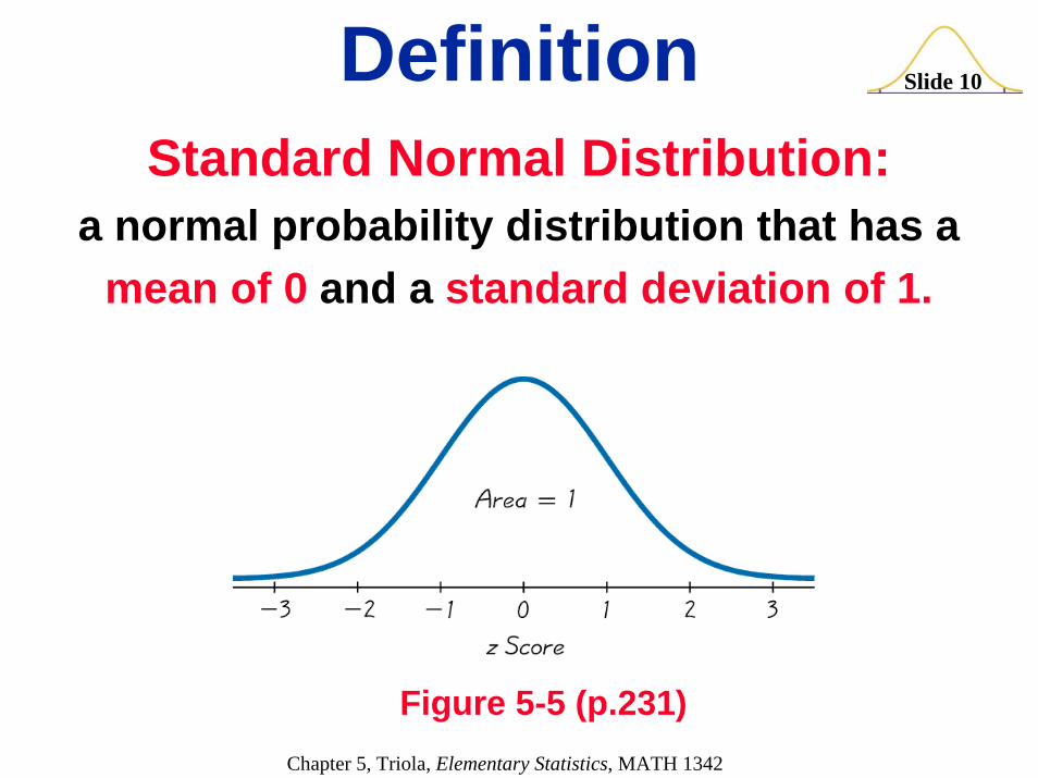
Example (p.232): If thermometers have an average (mean) reading of 0 degrees and a standard deviation of 1 degree for freezing water, and if one thermometer is randomly selected, find the probability that, at the freezing point of water, the reading is less than 1.58 degrees.

P(z < 1.58) =

Figure 5-6 (p.232)


Slide 15

Example: If thermometers have an average (mean) reading of 0 degrees and a standard deviation of 1 degree for freezing water and if one thermometer is randomly selected, find the probability that, at the freezing point of water, the reading is less than 1.58 degrees.

The probability that the chosen thermometer will measure freezing water less than 1.58 degrees is 0.9429.

P (z < 1.58) = 0.9429

Figure 5-6


Slide 16

Example: If thermometers have an average (mean) reading of 0 degrees and a standard deviation of 1 degree for freezing water and if one thermometer is randomly selected, find the probability that, at the freezing point of water, the reading is less than 1.58 degrees.

P (z < 1.58) = 0.9429

94.29% of the thermometers have readings less than 1.58 degrees.


Slide 17

Example: If thermometers have an average (mean) reading of 0 degrees and a standard deviation of 1 degree for freezing water, and if one thermometer is randomly selected, find the probability that it reads (at the freezing point of water) above –1.23 degrees.

The probability that the chosen thermometer with a reading above –1.23 degrees is 0.8907.

P (z > –1.23) = 0.8907


Slide 18

Example: If thermometers have an average (mean) reading of 0 degrees and a standard deviation of 1 degree for freezing water, and if one thermometer is randomly selected, find the probability that it reads (at the freezing point of water) above –1.23 degrees.

P (z > –1.23) = 0.8907

89.07% of the thermometers have readings above –1.23degrees.


Slide 19

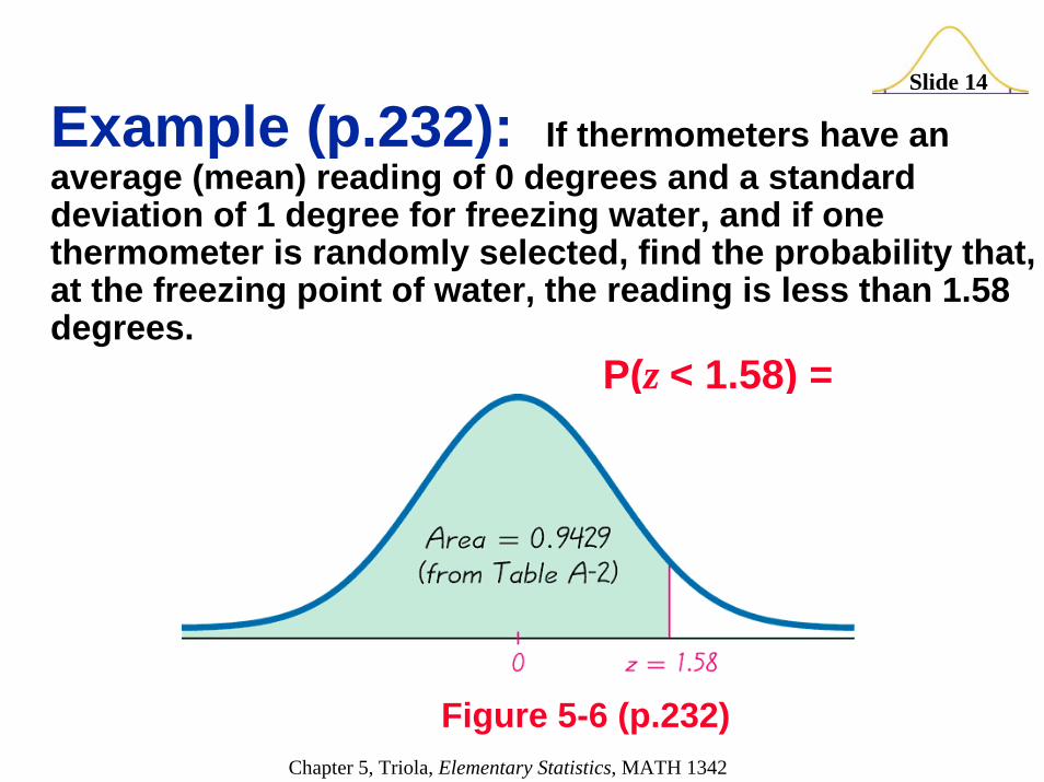
Example (p.233): A thermometer is randomly selected. Find the probability that it reads (at the freezing point of water) between –2.00 and 1.50 degrees.

P (z < –2.00) = 0.0228P (z < 1.50) = 0.9332P (–2.00 < z < 1.50) = 0.9332 – 0.0228 = 0.9104

The probability that the chosen thermometer has a reading between – 2.00 and 1.50 degrees is 0.9104.


Slide 20

Example: A thermometer is randomly selected. Find the probability that it reads (at the freezing point of water) between –2.00 and 1.50 degrees.

If many thermometers are selected and tested at the freezing point of water, then 91.04% of them will read between –2.00 and 1.50 degrees.

P (z < –2.00) = 0.0228P (z < 1.50) = 0.9332P (–2.00 < z < 1.50) = 0.9332 – 0.0228 = 0.9104


Slide 21

P(a < z < b) denotes the probability that the z score is

between a and bP(z > a)

denotes the probability that the z score is greater than aP(z < a)

denotes the probability that the z score is less than a

Notation (p.234)


Slide 22Finding a z - score when given a

probability Using Table A-2

1. Draw a bell-shaped curve, draw the centerline, and identify the region under the curve that corresponds to the given probability. If that region is not a cumulative region from the left, work instead with a known region that is a cumulative region from the left.

2. Using the cumulative area from the left, locate the closest probability in the body of Table A-2 and identify the corresponding z score.


Slide 23Finding z Scores

when Given Probabilities

Figure 5-10 (p.236)Finding the 95th Percentile

1.645

5% or 0.05

(z score will be positive)


Slide 24

Figure 5-11 (p.237) Finding the Bottom 2.5% and Upper 2.5%

(One z score will be negative and the other positive)

Finding z Scores when Given Probabilities

z


Slide 25


Section 5-3 Applications of Normal

Distributions


Slide 26Nonstandard Normal

DistributionsIf μ ≠ 0 or σ ≠ 1 (or both), we will convert values to standard scores using Formula 5-2, then procedures for working with all normal distributions are the same as those for the standard normal distribution.

Formula 5-2 (p.240)

x – µσz =


Slide 27

Figure 5-12 (p.240)

Converting to Standard Normal Distribution

x – μσz =


Slide 28

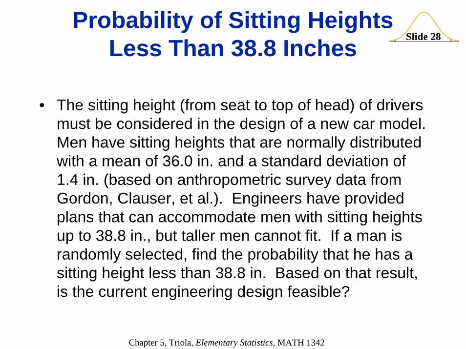
• The sitting height (from seat to top of head) of drivers must be considered in the design of a new car model. Men have sitting heights that are normally distributed with a mean of 36.0 in. and a standard deviation of 1.4 in. (based on anthropometric survey data from Gordon, Clauser, et al.). Engineers have provided plans that can accommodate men with sitting heights up to 38.8 in., but taller men cannot fit. If a man is randomly selected, find the probability that he has a sitting height less than 38.8 in. Based on that result, is the current engineering design feasible?

Probability of Sitting Heights Less Than 38.8 Inches


Slide 29Probability of Sitting Heights

Less Than 38.8 Inches

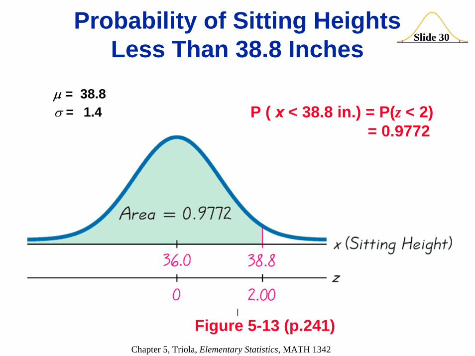
z = 38.8 – 36.01.4

= 2.00σ = 1.4 μ = 36.0

Figure 5-13 (p.241)


Slide 30Probability of Sitting Heights

Less Than 38.8 Inches

σ = 1.4 μ = 38.8

Figure 5-13 (p.241)

P ( x < 38.8 in.) = P(z < 2)= 0.9772


Slide 31

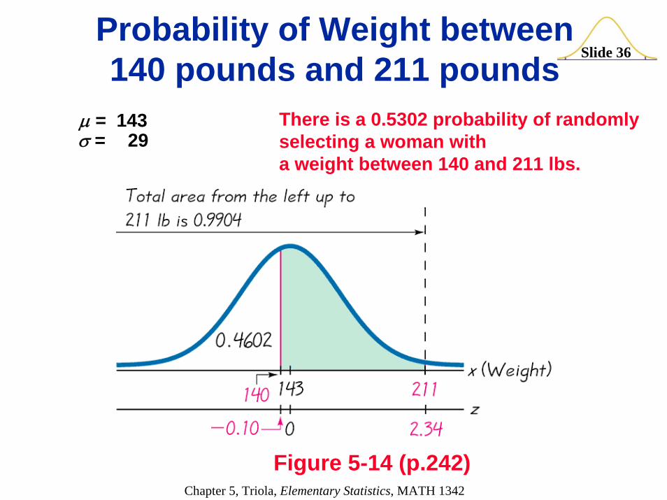
In the Chapter Problem, we noted that the Air Force had been using the ACES-II ejection seats designed for men weighing between 140 lb and 211 lb. Given that women’s weights are normally distributed with a mean of 143 lb and a standard deviation of 29 lb (based on data from the National Health survey), what percentage of women have weights that are within those limits?

Probability of Weight between 140 pounds and 211 pounds


Slide 32Probability of Weight between 140 pounds and 211 pounds

z = 211 – 14329

= 2.34σ = 29μ = 143

Figure 5-14 (p.242)



Figure 5-14 (p.242)

σ = 29μ = 143 z = 140 – 143

29= –0.10



Figure 5-14 (p.242)

σ = 29μ = 143 P( –0.10 < z < 2.34 ) =



Figure 5-14 (p.242)

σ = 29μ = 143 0.9904 – 0.4602 = 0.5302



Figure 5-14 (p.242)

σ = 29μ = 143 There is a 0.5302 probability of randomly

selecting a woman with a weight between 140 and 211 lbs.



σ = 29μ = 143

Figure 5-14 (p.242)

OR - 53.02% of women have weights between 140 lb and 211 lb.


Slide 38

1. Don’t confuse z scores and areas. z scores are distances along the horizontal scale, but areas are regions under the normal curve. Table A-2 lists z scores in the left column and across the top row, but areas are found in the body of the table.

2. Choose the correct (right/left) side of the graph. 3. A z score must be negative whenever it is located

to the left half of the normal distribution. 4. Areas (or probabilities) are positive or zero values,

but they are never negative.

Cautions to keep in mind


Slide 39Procedure for Finding Values

Using Table A-2 and Formula 5-21. Sketch a normal distribution curve, enter the given probability or

percentage in the appropriate region of the graph, and identify the xvalue(s) being sought.

2. Use Table A-2 to find the z score corresponding to the cumulative left area bounded by x. Refer to the BODY of Table A-2 to find the closest area, then identify the corresponding z score.

3. Using Formula 5-2, enter the values for µ, σ, and the z score found in step 2, then solve for x.

x = µ + (z • σ) (Another form of Formula 5-2)

(If z is located to the left of the mean, be sure that it is a negative number.)

4. Refer to the sketch of the curve to verify that the solution makes sense in the context of the graph and the context of the problem.


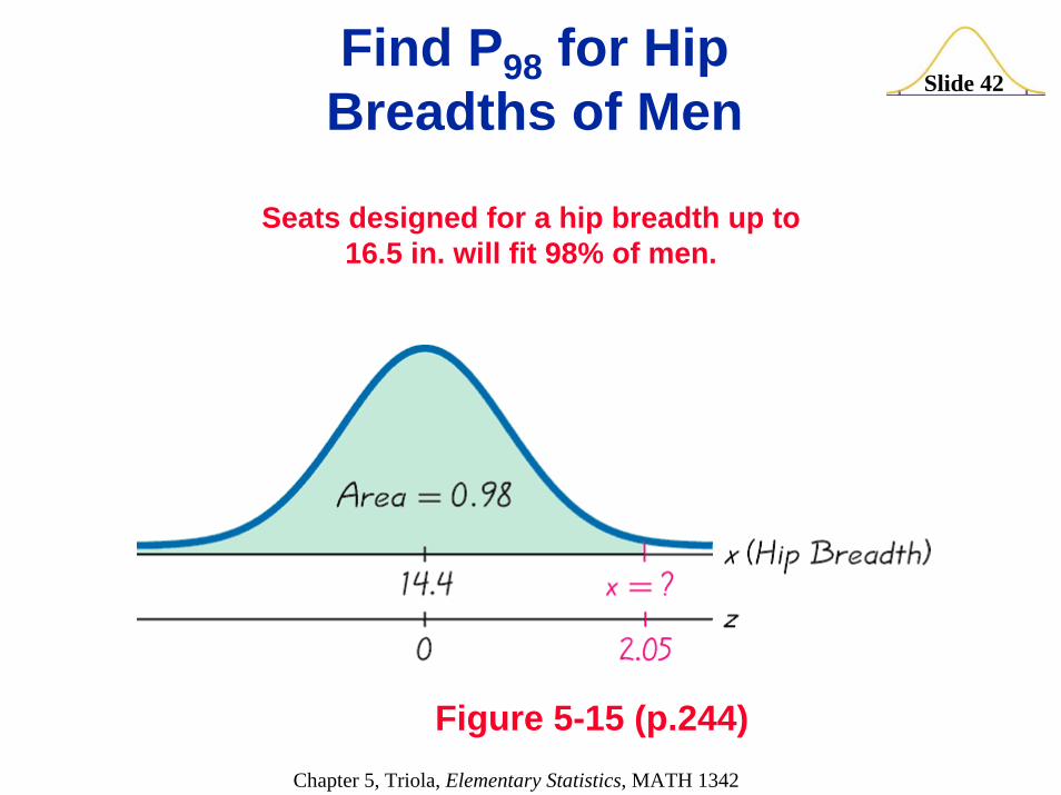
Slide 40Find P98 for Hip Breadths of Men

Figure 5-15 (p.244)

x = μ + (z ● σ)x = 14.4 + (2.05 • 1.0)x = 16.45



Figure 5-15 (p.244)

The hip breadth of 16.5 in. separates the lowest 98% from the highest 2%



Figure 5-15 (p.244)

Seats designed for a hip breadth up to 16.5 in. will fit 98% of men.


Slide 43

45% 50%

Figure 5-16 (p.245)

Finding P05 for Grips of Women

x = 27.0 + (–1.645 • 1.3) = 24.8615


Slide 44

45% 50%

Figure 5-16 (p.245)

Finding P05 for Grips of Women

The forward grip of 24.9 in. (rounded) separates the top 95% from the others.


Slide 45REMEMBER!

Make the z score negative if the value is located to the left (below) the mean. Otherwise, the z score will be positive.


Slide 46


Section 5-4Sampling Distributions

and Estimators


Slide 47

Sampling Distribution of the mean is the probability distribution of

sample means, with all samples having the same sample

size n.

Definition


Slide 48

Sampling Variability:The value of a statistic, such as the sample mean x, depends on the particular values included in the sample.

Definition


Slide 49

The Sampling Distribution of the Proportion is the probability distribution of sample proportions, with all samples having the same sample size n.

Definition


Slide 50

A population consists of the values 1, 2, and 5. We randomly select samples of size 2 with replacement. There are 9 possible samples.

a. For each sample, find the mean, median, range, variance, and standard deviation.

b. For each statistic, find the mean from part (a)

See Table 5-2 (p.251) on the next slide.

Sampling Distributions


Slide 51


Slide 52Interpretation of

Sampling Distributions

We can see that when using a sample statistic to estimate a population parameter, some statistics are good in the sense that they target the population parameter and are therefore likely to yield good results. Such statistics are called unbiased estimators.

Statistics that target population parameters: mean, variance, proportion

Statistics that do not target population parameters: median, range, standard deviation


Slide 53


Section 5-5The Central Limit

Theorem


Slide 54Central Limit Theorem

1. The random variable x has a distribution (which may or may not be normal) with mean µ and standard deviation σ.

2. Samples all of the same size n are randomly selected from the population of x values.

Given (p.260):


Slide 55

1. The distribution of sample x will, as the sample size increases, approach a normaldistribution.

2. The mean of the sample means will be the population mean µ.

3. The standard deviation of the sample means will approach σ/ . n

Conclusions (p.260):

Central Limit Theorem


Slide 56Practical Rules

Commonly Used:

1. For samples of size n larger than 30, the distribution of the sample means can be approximated reasonably well by a normal distribution. The approximation gets better as the sample size n becomes larger.

2. If the original population is itself normally distributed, then the sample means will be normally distributed for any sample size n (not just the values of n larger than 30).


Slide 57Notation (p.261)

the mean of the sample means

the standard deviation of sample mean

(often called standard error of the mean)

µx = µ

σx = σn


Slide 58Distribution of 200 digits from

Social Security Numbers(Last 4 digits from 50 students)

Figure 5-19 (p.262)


Slide 59


Slide 60Distribution of 50 Sample Means

for 50 Students

Figure 5-20 (p.262)


Slide 61

As the sample size increases, the sampling distribution of sample means approaches a

normal distribution.


Slide 62

Example (p.262): Given the population of men has normally distributed weights with a mean of 172 lb and a standard deviation of 29 lb,

a) if one man is randomly selected, find the probability that his weight is greater than 167 lb.

b) if 12 different men are randomly selected, find the probability that their mean weight is greater than 167 lb.


Slide 63

Example: Given the population of men has normally distributed weights with a mean of 172 lb and a standard deviation of 29 lb,


z = 167 – 172 = –0.1729


Slide 64


a) if one man is randomly selected, the probability that his weight is greater than 167 lb. is 0.5675.


Slide 65


b) if 12 different men are randomly selected, find the probability that their mean weight is greater than 167 lb.

z = 167 – 172 = –0.602936


Slide 66

z = 167 – 172 = –0.602936


b.) if 12 different men are randomly selected, the probability that their mean weight is greater than 167 lb is 0.7257.


Slide 67


b) if 12 different men are randomly selected, their mean weight is greater than 167 lb.

P(x > 167) = 0.7257It is much easier for an individual to deviate from the mean than it is for a group of 12 to deviate from the mean.


P(x > 167) = 0.5675


Slide 68Sampling Without

Replacement (p.266)

If n > 0.05 N

N – nσx = σn N – 1

finite populationcorrection factor


Slide 69


Section 5-6Normal as Approximation

to Binomial


Slide 70Review

Binomial Probability Distribution1. The procedure must have fixed number of trials.2. The trials must be independent.3. Each trial must have all outcomes classified into

two categories.4. The probabilities must remain constant for each

trial.

Solve by binomial probability formula, Table A-1, or technology


Slide 71Approximate a Binomial Distribution

with a Normal Distribution if:

np ≥ 5

nq ≥ 5

then µ = np and σ = npq

and the random variable has

distribution.(normal)

a


Slide 72

Figure 5-23

Solving Binomial

Probability Problems

Using a Normal

Approximation


Slide 73

12

3

4

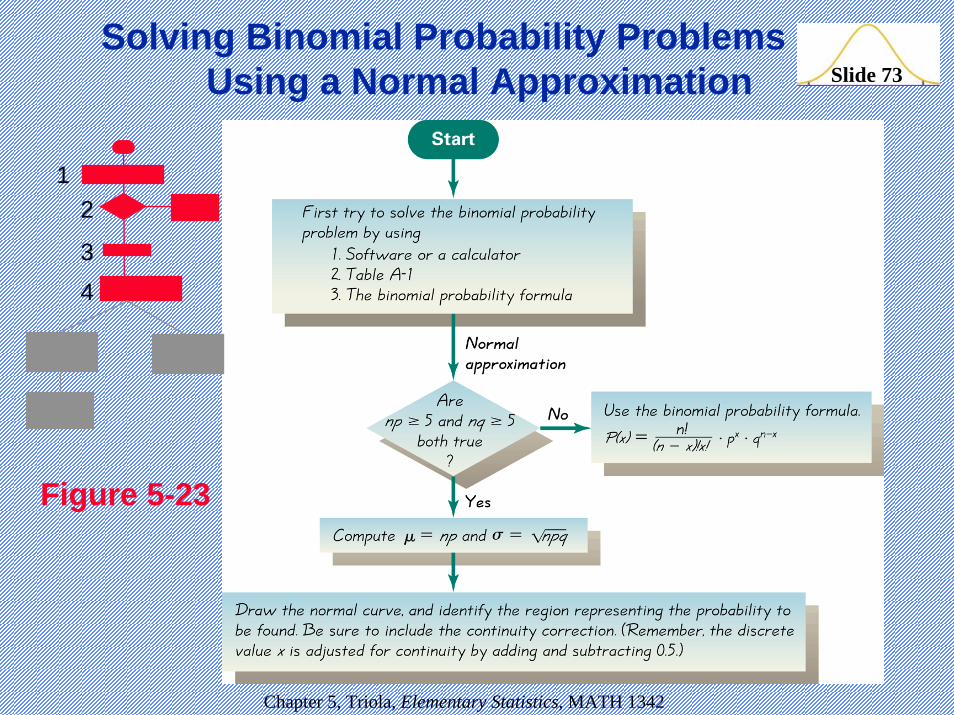
Figure 5-23

Solving Binomial Probability Problems Using a Normal Approximation


Slide 74Solving Binomial Probability Problems

Using a Normal Approximation

5

6

4 Use a TI-83 calculator

Figure 5-23


Slide 75Procedure for Using a Normal Distribution to Approximate

a Binomial Distribution1. Establish that the normal distribution is a suitable

approximation to the binomial distribution by verifying np ≥ 5 and nq ≥ 5.

2. Find the values of the parameters µ and σ by calculating µ = np and σ = npq.

3. Identify the discrete value of x (the number of successes). Change the discrete value x by replacing it with the interval from x – 0.5 to x + 0.5. Draw a normal curve and enter the values of µ , σ, and either x– 0.5 or x + 0.5, as appropriate.

continued


Slide 76

4. Change x by replacing it with x – 0.5 or x + 0.5, as appropriate.

5. Find the area corresponding to the desired probability.

continued

Procedure for Using a Normal Distribution to Approximate

a Binomial Distribution


Slide 77

Figure 5-24

Finding the Probability of “At Least”

120 Men Among 200 Accepted Applicants


Slide 78DefinitionWhen we use the normal distribution

(which is continuous) as an approximation to the binomial

distribution (which is discrete), a continuity correction is made to a

discrete whole number x in the binomial distribution by representing the single

value x by the interval from x – 0.5 to x + 0.5.


Slide 79Procedure for

Continuity Corrections 1. When using the normal distribution as an approximation to the

binomial distribution, always use the continuity correction.

2. In using the continuity correction, first identify the discrete whole number x that is relevant to the binomial probability problem.

3. Draw a normal distribution centered about µ, then draw a vertical strip area centered over x . Mark the left side of the strip with the

number x – 0.5, and mark the right side with x + 0.5. For x =120, draw a strip from 119.5 to 120.5. Consider the area of the strip to represent the probability of discrete number x.

continued


Slide 80

4. Now determine whether the value of x itself should be included in the probability you want. Next, determine whether you want the probability of at least x, at most x, more than x, fewer than x, or

exactly x. Shade the area to the right or left of the strip, as

appropriate; also shade the interior of the strip itself if and only if xitself is to be included. The total shaded region corresponds to probability being sought.

continued

Procedure for Continuity Corrections


Slide 81

Figure 5-25

x = at least 120= 120, 121, 122, . . .

x = more than 120= 121, 122, 123, . . .

x = at most 120= 0, 1, . . . 118, 119, 120

x = fewer than 120= 0, 1, . . . 118, 119


Slide 82x = exactly 120

Interval represents discrete number 120


Slide 83


Section 5-7Determining Normality


Slide 84Definition

A Normal Quantile Plot is a graph of points (x,y), where each x value is from the original set of sample data, and each y value is a z score corresponding to a quantile value of the standard normal distribution.


Slide 85Procedure for Determining

Whether Data Have a Normal Distribution

1. Histogram: Construct a histogram. Reject normality if the histogram departs dramatically from a bell shape.

2. Outliers: Identify outliers. Reject normality if there is more than one outlier present.

3. Normal Quantile Plot: If the histogram is basically symmetric and there is at most one outlier, construct a normal quantile plot as follows:


Slide 86

a. Sort the data by arranging the values from lowest to highest.

b. With a sample size n, each value represents a proportion of 1/nof the sample. Using the known sample size n, identify the areas of 1/2n, 3/2n, 5/2n, 7/2n, and so on. These are the cumulative areas to the left of the corresponding sample values.

c. Use the standard normal distribution (Table A-2) to find the zscores corresponding to the cumulative left areas found in Step (b).

continued

3. Normal Quantile Plot

Procedure for Determining Whether Data Have a Normal Distribution


Slide 87

d. Match the original sorted data values with their corresponding z scores found in Step (c), then plot the points (x, y), where each x is an original sample value and y is the corresponding z score.

e. Examine the normal quantile plot using these criteria:If the points do not lie close to a straight line, or if the points exhibit some systematic pattern that is not a straight-line pattern, then the data appear to come from a population that does not have a normal distribution. If the pattern of the points is reasonably close to a straight line, then the data appear to come from a population that has a normal distribution.

continued



Slide 88

Examine the normal quantile plot and reject normality if the the points do not

lie close to a straight line, or if the points exhibit some systematic pattern that is

not a straight-line pattern.


4-5 The Poisson Distribution

Documents