4 - 0 4.1. Levels of Image Data Representation 4.2. Traditional Image Data Structures 4.3. Hierarchical Data Structures Chapter 4 – Data structures for.

4 - 1

4.1. Levels of Image Data Representation

4.2. Traditional Image Data Structures

4.3. Hierarchical Data Structures

Chapter 4 – Data structures for image analysis

4 - 2

4.1. Levels of Image Data Representation

(i) Pixel-level representation

Intensity image

Range image

4 - 3

Color image

Indexed (or palette) color image

4 - 4

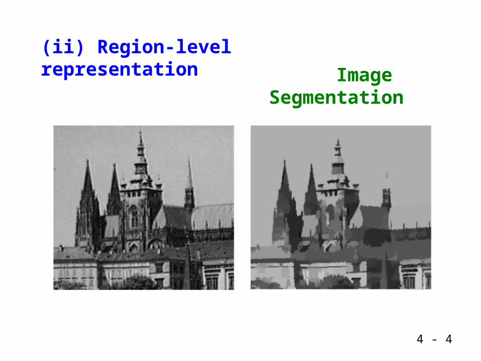
(ii) Region-level representation

Image Segmentation

4 - 5

(iii) Abstract level representation

Region adjacency graphs

Semantic nets

Segmented Image

Binary Image

4 - 6

4.2. Traditional Image Data Structures

4.2.1. Matrices

Matrices, chains, graphs, tables

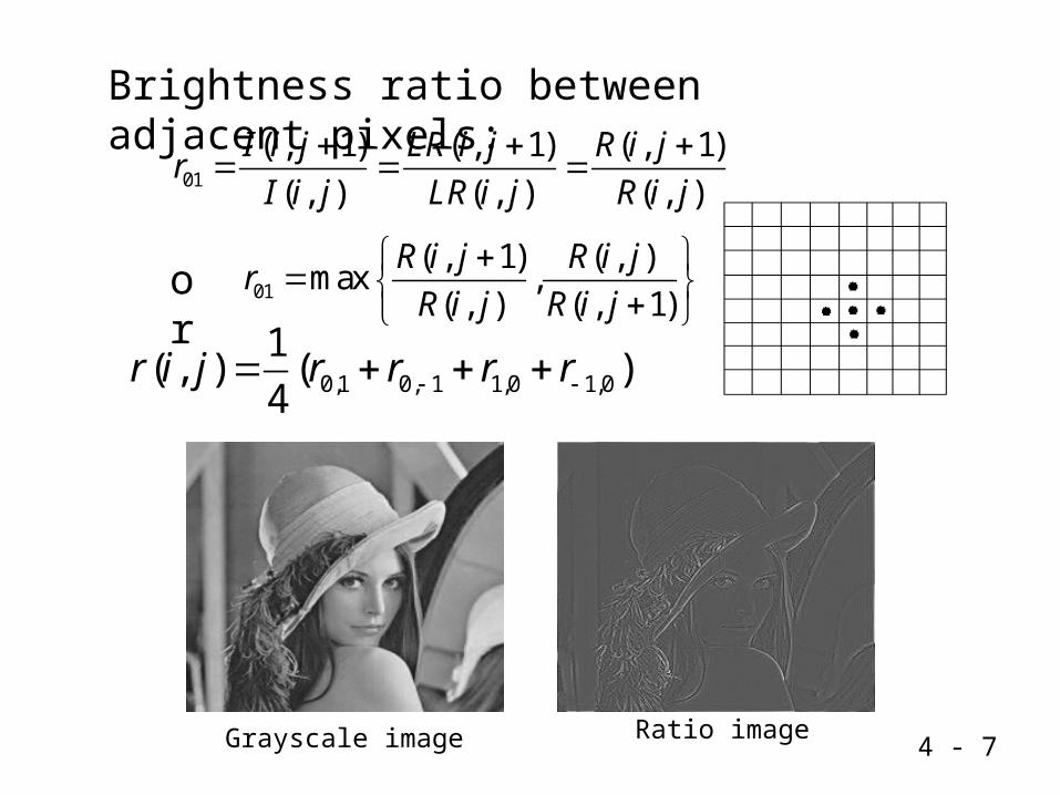
(i) Ratio image – removes the effect of illumination variation

( , ) ( , )I i j LR i jImage model:

4 - 7

0,1 0, 1 1,0 1,0

1( , ) ( )

4r i j r r r r

01

( , 1) ( , 1) ( , 1)

( , ) ( , ) ( , )

I i j LR i j R i jr

I i j LR i j R i j

Brightness ratio between adjacent pixels:

or

Grayscale image Ratio image

01

( , 1) ( , )max ,

( , ) ( , 1)

R i j R i jr

R i j R i j

4 - 8

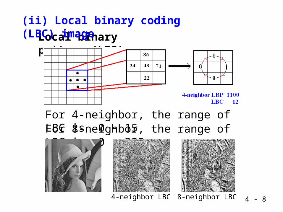
Local binary pattern (LBP)

(ii) Local binary coding (LBC) image

For 4-neighbor, the range of LBC is 0 - 15For 8-neighbor, the range of LBC is 0 - 255

4-neighbor LBC 8-neighbor LBC

4 - 9

Intrinsic Image Extraction

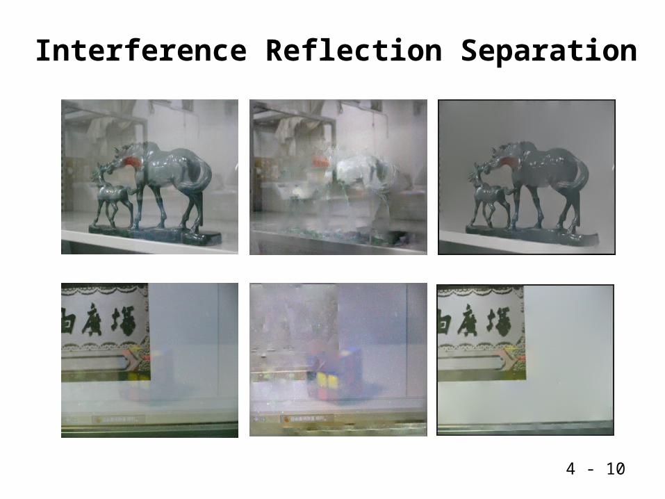
Interference Reflection Separation

4 - 10

4 - 11

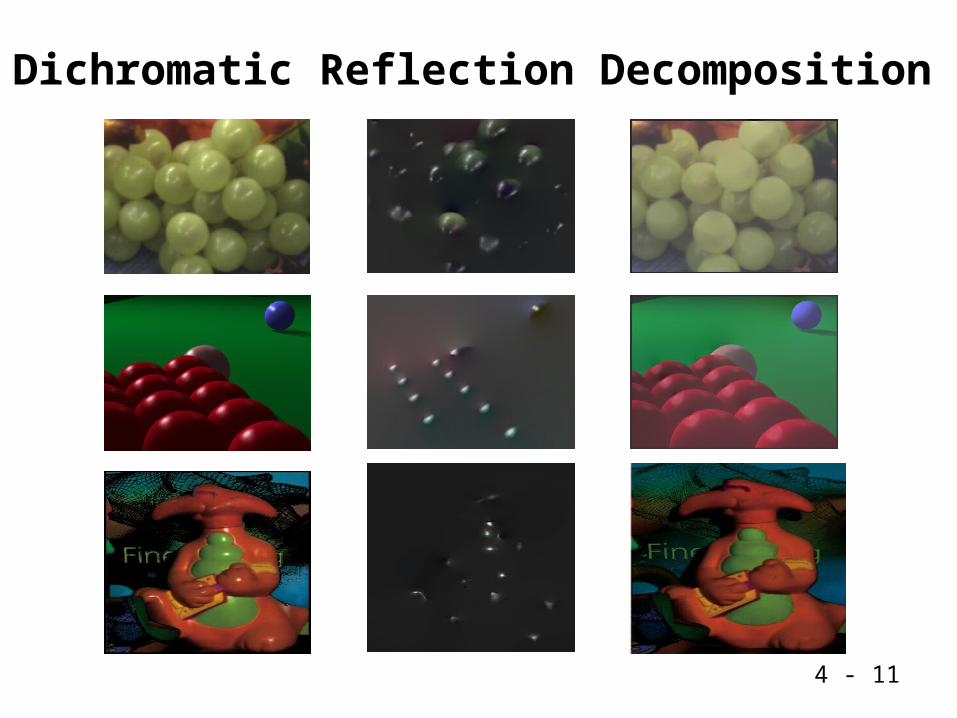
Dichromatic Reflection Decomposition

Dehaze

4 - 13

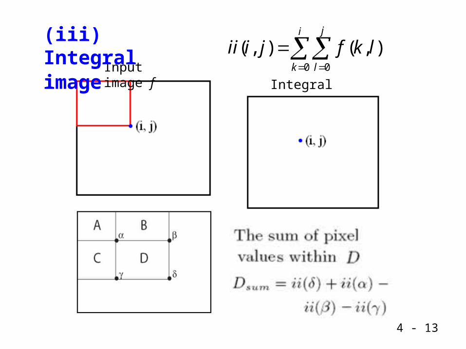
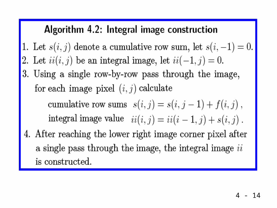
Integral image ii

0 0

( , ) ( , )ji

k l

ii i j f k l

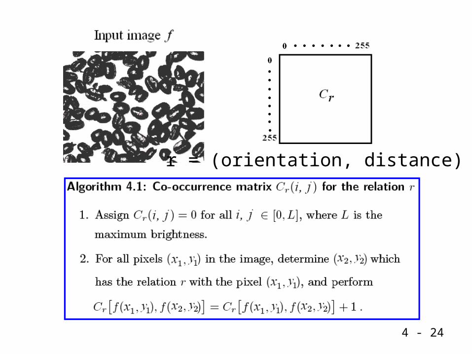
Input image f

(iii) Integral image

4 - 14

4 - 15

Application: Face location

4 - 16

4 - 17

Adaboost (learning) algorithm (10.6)

1 2( ,1), ( ,1), , ( ,1)mx x x

n training samples:

i x X 0,1iy Y : data space, : label space

tD

m positive samples:

l negative samples: 1 2( ,0), ( ,0), , ( ,0)m m m l x x x

( , )i iyx

4 - 18

1 2{ , , , }nF f f fFeature set:

1 2{ , , , }nH h h h Classifier set associated with F:

Sample’s distribution at time t :

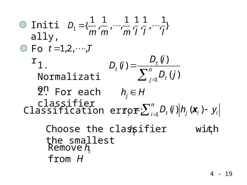
For 1,2, ,t T

1. Normalization 1

( )( )

( )t

t n

tj

D iD i

D j

4 - 19

2. For each classifier jh H

1( ) ( )

n

j t j i iiD i h y

xClassification error:

Choose the classifier with the smallestth t

Remove from Hth

Initially,

1

1 1 1 1 1 1{ , , , , , , , }D

m m m l l l

1logt

t

Construct the strong classifier

1 1

11 ( )

( ) 2

0 otherwise

T T

t t tt t

hH

xx

where

Extension: Cascaded adaboost algorithm

4 - 20

1t

tt

1

( )( ) ( )

1 ( )t t i i

t tt i i

h yD i D i

h y

x

x

3. Update

where

4 - 21

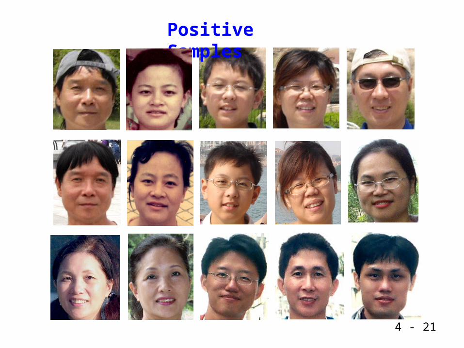
Positive Samples

4 - 22

Negative Samples

4 - 23

(iv) Co-occurrence matrix (or Spatial gray-level

dependence matrix)Texture analysis

Texture: closely interwoven elements

4 - 24

r = (orientation, distance)

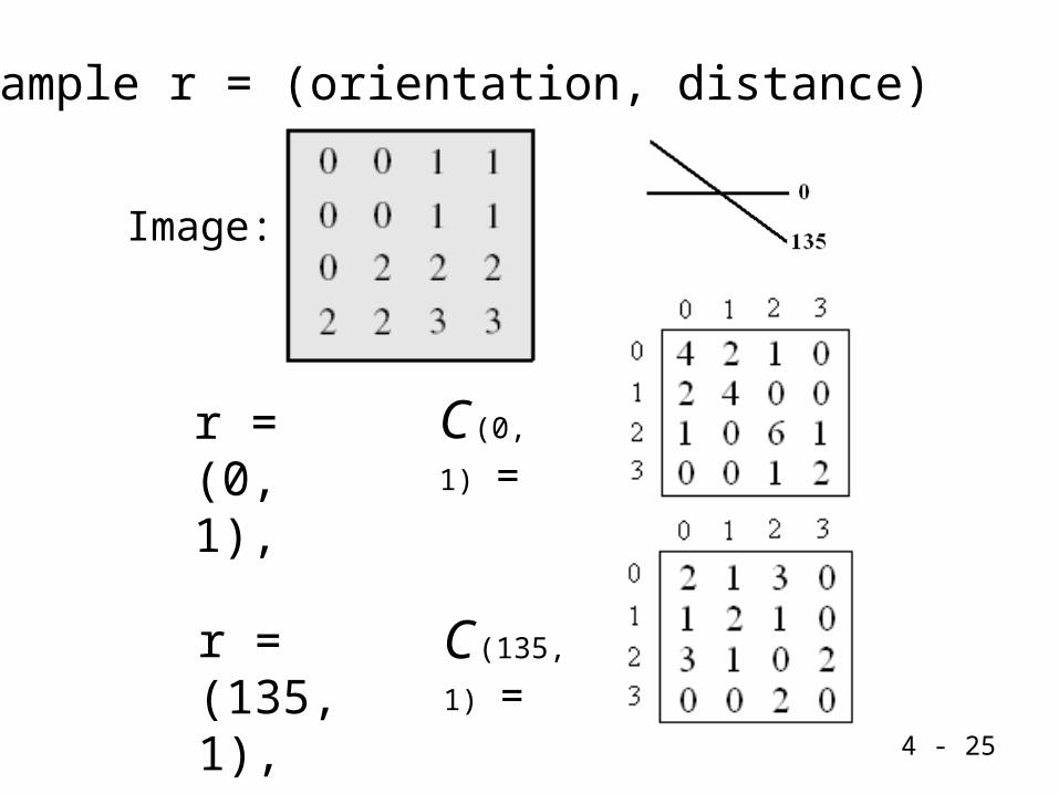
Example r = (orientation, distance)

Image:

r = (0, 1), C (0, 1) =

r = (135, 1), C (135, 1)

= 4 - 25

4 - 26

Potential features calculated from co-occurrence matrices

1 12

0 0

( ) ( , )L L

ri j

E r C i j

Energy:

1 1

0 0

( ) ( , ) log ( , )L L

r ri j

H r C i j C i j

Entropy:

Correlation:1 1

2

0 0

( ) ( ) ( , )L L

ri j

I r i j C i j

Homogeneity:

1 1

0 0

2

( , )

( )1 ( )

L L

ri j

C i j

L ri j

4 - 27

Inertia:

1 1

0 0

( )( ) ( , )

( )

L L

x y ri j

x y

i j C i j

C r

1 1

0 0

( , )L L

x ri j

i C i j

1 1

0 0

( , )L L

y rj i

j C i j

1 12 2

0 0

( ) ( , ),L L

x x ri j

i C i j

1 12 2

0 0

( ) ( , )L L

y y rj i

j C i j

where

4 - 28

Feature vector formed from features

e.g., ( ) ( , , , , )r E H I L Cv

1 2, , , nr r rDifferent relations

4 - 29

4.2.2. Chains

(i)Chain code: for description of object borders

4 - 30

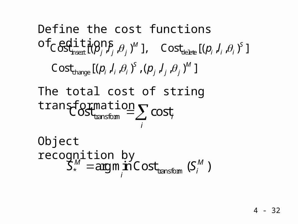
(ii) Attributed strings

1 1 1 2 2 2( , , )( , , ) ( , , )n n nS p l p l p l

where : polyline, : length, : directionp l

4 - 31

String matching

1 1 1 2 2 2( , , ) ( , , ) ( , , )S S S Sm m mS p l p l p l Scene

string: Model string:

1 1 1 2 2 2( , , ) ( , , ) ( , , )M M M Mn n nS p l p l p l

Types of edition: insert, delete, change

Calculate the cost of transforming toSS MS

String transformation through editions

The larger the cost the larger the difference between

the two strings, and in turn the larger the difference

between the two shapes described by the strings.

4 - 32

Define the cost functions of editions

insertCost [( , , ) ],Mj j jp l deleteCost [( , , ) ]S

i i ip l

changeCost [( , , ) , ( , , ) ]S Mi i i j j jp l p l

The total cost of string transformation

transformCost cost ii

Object recognition by

* transformarg min Cost ( )M Mi

iS S

4 - 33

(iii) Run length code: to represent strings of symbols in an image (e.g., for transmission)Binary images:(Row#, (beginning col., end col.) .... (beginning col., end col.)) ………………………………………(Row#, (beginning col., end col.) .... (beginning col., end col.))

Gray level images:(Row#, (beginning col., end col., brightness) .... (beginning col., end col., brightness)) …………....…………………. (Row#, (beginning col., end col., brightness) .... (beginning col., end col., brightness))

4 - 34

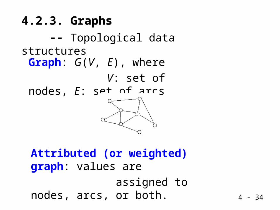
4.2.3. Graphs

-- Topological data structures

Graph: G(V, E), where

V: set of nodes, E: set of arcs

Attributed (or weighted) graph: values are

assigned to nodes, arcs, or both.

4 - 35

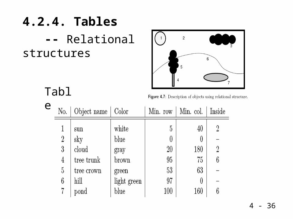
Region adjacency graphs

Semantic nets

Images are described as a set of elements and

their relations.

4 - 36

4.2.4. Tables

-- Relational structures

Table

4 - 37

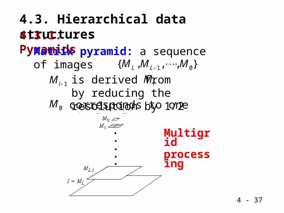
4.3. Hierarchical data structures4.3.1. Pyramids

Matrix pyramid: a sequence of images1 0{ , , , }L LM M M

0M

1iM is derived from by reducing the resolution by 1/2

iM

corresponds to one pixel only

Multigrid processing

4 - 38

the set of nodes at level k

{( , , ) | , [0, 2 1]}, [0, ] :kkP k i j i j k L

Let : the size of an image2L

Tree pyramid:

4 - 39

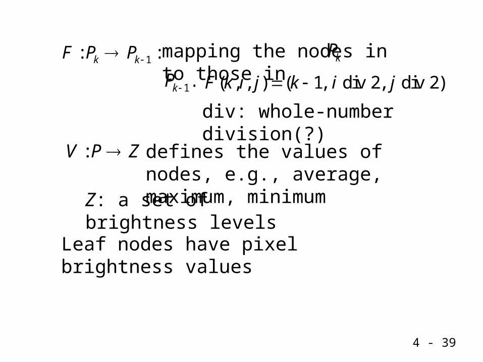
1: :k kF P P

Z: a set of brightness levels

:V P Z

mapping the nodes in to those in

( , , ) ( 1, div 2, div 2)F k i j k i j

Leaf nodes have pixel brightness values

defines the values of nodes, e.g., average, maximum, minimum

div: whole-number division(?)

1.kP

kP

4 - 40

e.g.,

{(1,0,0), (1,0,1), (1,1,0), (1,1,1)}

(1,0,1) (0,0,0),F

(1,1,1) (0,0,0)F (1,1,0) (0,0,0),F

, [0, 2 1] [0,1]ki j

{( , , ) | , [0, 2 1]}kkP k i j i j

( , , ) ( 1, div 2, div 2)F k i j k i j

1 {(1, , ) | , [0,1]}P i j i j

00, {(0, , ) | , [0,0]} {(0,0,0)}k P i j i j

From

From

k = 1,

(1,0,0) (0,0,0),F

4 - 41

k = 2,

2 {(2,0,0), (2,0,1), (2,0,2), (2,0,3), (2,1,0), (2,1,1),

(2,1,2), (2,1,3), (2,2,0), (2,2,1), (2,2,2), (2,2,3),

(2,3,0), (2,3,1), (2,3,2), (2,3,3)}

P

, [0, 2 1] [0,3]ki j

( , , ) ( 1, div 2, div 2)F k i j k i j

(2,1, 2) (1,0,1),F e.g.,

(2,3,1) (1,1,1)F

{( , , ) | , [0, 2 1]}kkP k i j i j From

4 - 42

4.3.2. Quadtrees

4 - 43

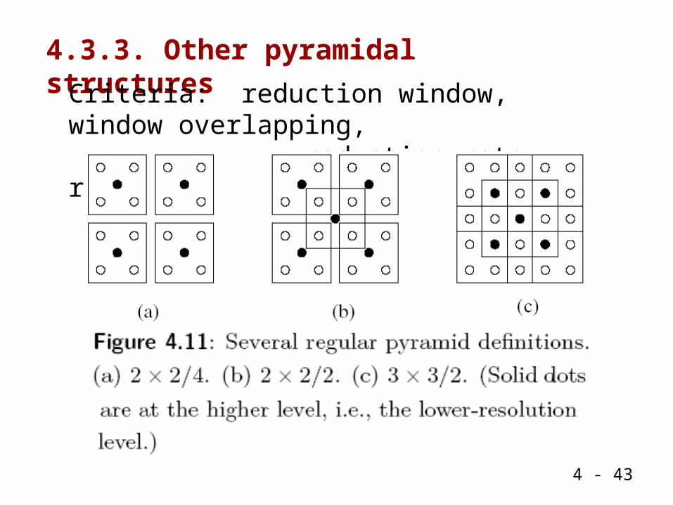
4.3.3. Other pyramidal structures

Criteria: reduction window, window overlapping, reduction rate, regularity