3D video-based deformation measurement of the pelvis bone under dynamic cyclic loading

RESEARCH Open Access

3D video-based deformation measurement of thepelvis bone under dynamic cyclic loadingBeat Göpfert1*, Zdzislaw Krol2, Marie Freslier3 and Andreas H Krieg2

* Correspondence: [email protected] of Biomechanics &Biocalorimetry, CM&BE, Universityof Basel, c/o Bio/Pharmazentrum,Klingelbergstrasse 50-70, 4056Basel, SwitzerlandFull list of author information isavailable at the end of the article

Abstract

Background: Dynamic three-dimensional (3D) deformation of the pelvic bones is acrucial factor in the successful design and longevity of complex orthopaediconcological implants. The current solutions are often not very promising for thepatient; thus it would be interesting to measure the dynamic 3D-deformation of thewhole pelvic bone in order to get a more realistic dataset for a better implantdesign. Therefore we hypothesis if it would be possible to combine a materialtesting machine with a 3D video motion capturing system, used in clinical gaitanalysis, to measure the sub millimetre deformation of a whole pelvis specimen.

Method: A pelvis specimen was placed in a standing position on a material testingmachine. Passive reflective markers, traceable by the 3D video motion capturingsystem, were fixed to the bony surface of the pelvis specimen. While applying adynamic sinusoidal load the 3D-movement of the markers was recorded by thecameras and afterwards the 3D-deformation of the pelvis specimen was computed.The accuracy of the 3D-movement of the markers was verified with 3D-displacementcurve with a step function using a manual driven 3D micro-motion-stage.

Results: The resulting accuracy of the measurement system depended on thenumber of cameras tracking a marker. The noise level for a marker seen by twocameras was during the stationary phase of the calibration procedure ± 0.036 mm,and ± 0.022 mm if tracked by 6 cameras. The detectable 3D-movement performedby the 3D-micro-motion-stage was smaller than the noise level of the 3D-videomotion capturing system. Therefore the limiting factor of the setup was the noiselevel, which resulted in a measurement accuracy for the dynamic test setup of ±0.036 mm.

Conclusion: This 3D test setup opens new possibilities in dynamic testing of widerange materials, like anatomical specimens, biomaterials, and its combinations. Theresulting 3D-deformation dataset can be used for a better estimation of materialcharacteristics of the underlying structures. This is an important factor in a reliablebiomechanical modelling and simulation as well as in a successful design of compleximplants.

Göpfert et al. BioMedical Engineering OnLine 2011, 10:60http://www.biomedical-engineering-online.com/content/10/1/60

© 2011 Göpfert et al; licensee BioMed Central Ltd. This is an Open Access article distributed under the terms of the Creative CommonsAttribution License (http://creativecommons.org/licenses/by/2.0), which permits unrestricted use, distribution, and reproduction inany medium, provided the original work is properly cited.

BackgroundVideo motion capturing (MoCap) systems are widely used in animation industries and

also in biomechanical applications with the main focus of macroscopic gait analysis

[1]. Due to systems improvements over the last years, they are now capable of resolu-

tions of 4704 × 3456 pixels (T160, Vicon, Oxford, UK) and sampling rates up to 10000

frames per second (Raptor 4, Motion Analysis Corporation, Santa Rosa, CA, USA).

This increased technology opens new application areas where high camera resolution

is needed such as in measuring small deformations of biological tissues, dynamic

three-dimensional (3D) deformation of bone-implant systems, or to determine move-

ment after fracture fixation [2-6]. Further, micro motion between bone and implant is

an important factor in the longevity of a stable bone-implant interface [7-9]. In parti-

cular, the characteristics of complex implant systems with bio-absorbable materials or

bioactive surface coatings are not completely known [10]. Variation in daily activities

may alter the loading conditions in the bone-implant system because of changing

material properties on one hand and the influences of operations on the other. How-

ever, biomechanical loading tests can never cover the whole variety of different loading

conditions during daily activity or consider all the changes over time in the biological

or implant structure [11]. Although computation-based modelling tries to include in

its calculation process changes of the bone-implant system; its original data must be

based on real validated measurements otherwise it can lead to false conclusions

[12,13]. Nevertheless local deformation can be measured highly precise with strain

gauges [14,15], or linear variable differential transducers [16]. To measure the

3D-deformation of a whole specimen other methods give a better spatial resolution.

Therefore the hypothesis was that a three-dimensional video MoCap system has the

potential to measure the sub millimetre 3D-deformation of a whole pelvis specimen.

This study describes the application of dynamic 3D-deformation measurement using

a 3D video MoCap system to gain data for the development of complex orthopaedic

oncological implants around the hip joint of the pelvis including the determination of

its accuracy with a 3D micrometre stage. The measurement of 3D-deformation was

done by recording the 3D-movement of passive reflective markers glued onto bone

surface while applying a dynamic, cyclic, non-constrained, uni-axial load to the pelvic

bone. The results will help achieve more stable implant fixation to the bone, which

improves the initial conditions for successful osseointegration and therefore support

the durability of the implant in a complex environment after a reconstructive surgery

for bone tumour.

MethodsDetermination of the accuracy of the 3D motion-capture system

The accuracy of the measurement setup was determined under the same conditions as

the pelvis specimen test was performed. A rigid steel framework equipped with 10 digital

high-speed cameras (6 cameras Vicon MX13+, 4 cameras Vicon T40, Vicon, Oxford,

UK) was placed around a Servo-hydraulic testing machine (MTS Bionix 858, MTS Eden

Prairie, MN, USA). The framework was screwed to the concrete floor and walls of the

room to avoid movement of the cameras and have the 10 cameras in the same stable

position during measurements. A 3D linear stage (M-461-XYZ-M, Newport Spectra-

Physics GmbH, Darmstadt, Germany) equipped with three manually-driven differential

Göpfert et al. BioMedical Engineering OnLine 2011, 10:60http://www.biomedical-engineering-online.com/content/10/1/60

Page 2 of 13

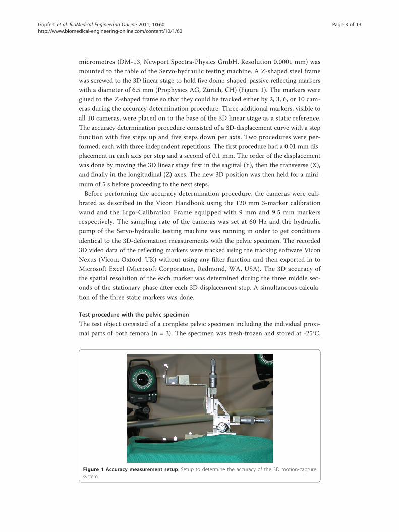
micrometres (DM-13, Newport Spectra-Physics GmbH, Resolution 0.0001 mm) was

mounted to the table of the Servo-hydraulic testing machine. A Z-shaped steel frame

was screwed to the 3D linear stage to hold five dome-shaped, passive reflecting markers

with a diameter of 6.5 mm (Prophysics AG, Zürich, CH) (Figure 1). The markers were

glued to the Z-shaped frame so that they could be tracked either by 2, 3, 6, or 10 cam-

eras during the accuracy-determination procedure. Three additional markers, visible to

all 10 cameras, were placed on to the base of the 3D linear stage as a static reference.

The accuracy determination procedure consisted of a 3D-displacement curve with a step

function with five steps up and five steps down per axis. Two procedures were per-

formed, each with three independent repetitions. The first procedure had a 0.01 mm dis-

placement in each axis per step and a second of 0.1 mm. The order of the displacement

was done by moving the 3D linear stage first in the sagittal (Y), then the transverse (X),

and finally in the longitudinal (Z) axes. The new 3D position was then held for a mini-

mum of 5 s before proceeding to the next steps.

Before performing the accuracy determination procedure, the cameras were cali-

brated as described in the Vicon Handbook using the 120 mm 3-marker calibration

wand and the Ergo-Calibration Frame equipped with 9 mm and 9.5 mm markers

respectively. The sampling rate of the cameras was set at 60 Hz and the hydraulic

pump of the Servo-hydraulic testing machine was running in order to get conditions

identical to the 3D-deformation measurements with the pelvic specimen. The recorded

3D video data of the reflecting markers were tracked using the tracking software Vicon

Nexus (Vicon, Oxford, UK) without using any filter function and then exported in to

Microsoft Excel (Microsoft Corporation, Redmond, WA, USA). The 3D accuracy of

the spatial resolution of the each marker was determined during the three middle sec-

onds of the stationary phase after each 3D-displacement step. A simultaneous calcula-

tion of the three static markers was done.

Test procedure with the pelvic specimen

The test object consisted of a complete pelvic specimen including the individual proxi-

mal parts of both femora (n = 3). The specimen was fresh-frozen and stored at -25°C.

Figure 1 Accuracy measurement setup. Setup to determine the accuracy of the 3D motion-capturesystem.

Göpfert et al. BioMedical Engineering OnLine 2011, 10:60http://www.biomedical-engineering-online.com/content/10/1/60

Page 3 of 13

After thawing to room temperature, soft tissues were removed cautiously, leaving the

joint capsule, the ventral and dorsal sacroiliac ligaments, the sacrotuberal and sacrosp-

inal ligaments, and the obturator membrane intact. The femora were then fixed with

polymethyl methacrylate (PMMA, Beracryl, Swiss-composite, Jegenstorf, CH) in the

holding fixture, which was mounted on the table of the Servo-hydraulic testing

machine to simulate a two-leg standing position. The load was applied vertically onto

the sacrum by the axial actuator of the testing machine with an adjustable fixture at

the sacrum, allowing unconstrained rotational and transverse motion [17]. After adjust-

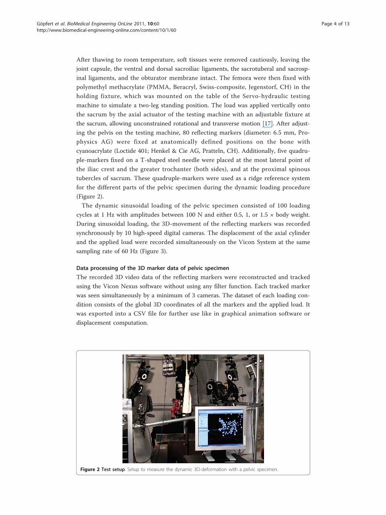
ing the pelvis on the testing machine, 80 reflecting markers (diameter: 6.5 mm, Pro-

physics AG) were fixed at anatomically defined positions on the bone with

cyanoacrylate (Loctide 401; Henkel & Cie AG, Pratteln, CH). Additionally, five quadru-

ple-markers fixed on a T-shaped steel needle were placed at the most lateral point of

the iliac crest and the greater trochanter (both sides), and at the proximal spinous

tubercles of sacrum. These quadruple-markers were used as a ridge reference system

for the different parts of the pelvic specimen during the dynamic loading procedure

(Figure 2).

The dynamic sinusoidal loading of the pelvic specimen consisted of 100 loading

cycles at 1 Hz with amplitudes between 100 N and either 0.5, 1, or 1.5 × body weight.

During sinusoidal loading, the 3D-movement of the reflecting markers was recorded

synchronously by 10 high-speed digital cameras. The displacement of the axial cylinder

and the applied load were recorded simultaneously on the Vicon System at the same

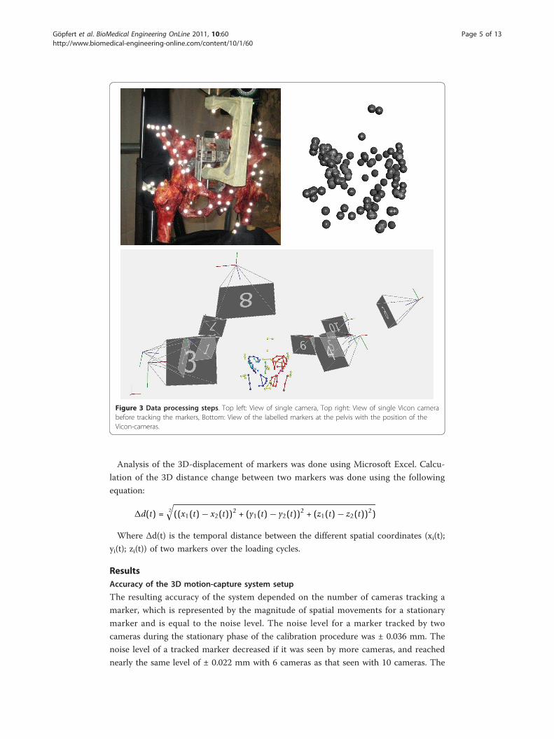
sampling rate of 60 Hz (Figure 3).

Data processing of the 3D marker data of pelvic specimen

The recorded 3D video data of the reflecting markers were reconstructed and tracked

using the Vicon Nexus software without using any filter function. Each tracked marker

was seen simultaneously by a minimum of 3 cameras. The dataset of each loading con-

dition consists of the global 3D coordinates of all the markers and the applied load. It

was exported into a CSV file for further use like in graphical animation software or

displacement computation.

Figure 2 Test setup. Setup to measure the dynamic 3D-deformation with a pelvic specimen.

Göpfert et al. BioMedical Engineering OnLine 2011, 10:60http://www.biomedical-engineering-online.com/content/10/1/60

Page 4 of 13

Analysis of the 3D-displacement of markers was done using Microsoft Excel. Calcu-

lation of the 3D distance change between two markers was done using the following

equation:

�d(t) = 2

√((x1(t) − x2(t))2 + (y1(t) − y2(t))2 + (z1(t) − z2(t))2)

Where Δd(t) is the temporal distance between the different spatial coordinates (xi(t);

yi(t); zi(t)) of two markers over the loading cycles.

ResultsAccuracy of the 3D motion-capture system setup

The resulting accuracy of the system depended on the number of cameras tracking a

marker, which is represented by the magnitude of spatial movements for a stationary

marker and is equal to the noise level. The noise level for a marker tracked by two

cameras during the stationary phase of the calibration procedure was ± 0.036 mm. The

noise level of a tracked marker decreased if it was seen by more cameras, and reached

nearly the same level of ± 0.022 mm with 6 cameras as that seen with 10 cameras. The

Figure 3 Data processing steps. Top left: View of single camera, Top right: View of single Vicon camerabefore tracking the markers, Bottom: View of the labelled markers at the pelvis with the position of theVicon-cameras.

Göpfert et al. BioMedical Engineering OnLine 2011, 10:60http://www.biomedical-engineering-online.com/content/10/1/60

Page 5 of 13

noise level of the 3D position of the static markers tracked by all 10 cameras was ±

0.020 mm (Table 1).

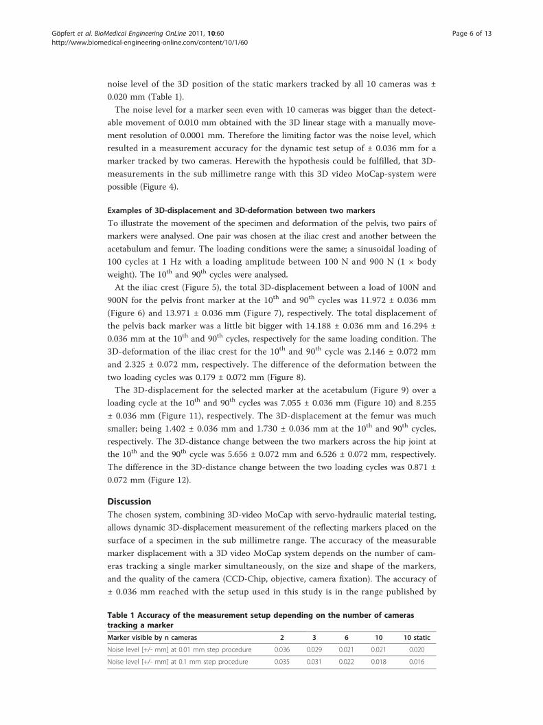
The noise level for a marker seen even with 10 cameras was bigger than the detect-

able movement of 0.010 mm obtained with the 3D linear stage with a manually move-

ment resolution of 0.0001 mm. Therefore the limiting factor was the noise level, which

resulted in a measurement accuracy for the dynamic test setup of ± 0.036 mm for a

marker tracked by two cameras. Herewith the hypothesis could be fulfilled, that 3D-

measurements in the sub millimetre range with this 3D video MoCap-system were

possible (Figure 4).

Examples of 3D-displacement and 3D-deformation between two markers

To illustrate the movement of the specimen and deformation of the pelvis, two pairs of

markers were analysed. One pair was chosen at the iliac crest and another between the

acetabulum and femur. The loading conditions were the same; a sinusoidal loading of

100 cycles at 1 Hz with a loading amplitude between 100 N and 900 N (1 × body

weight). The 10th and 90th cycles were analysed.

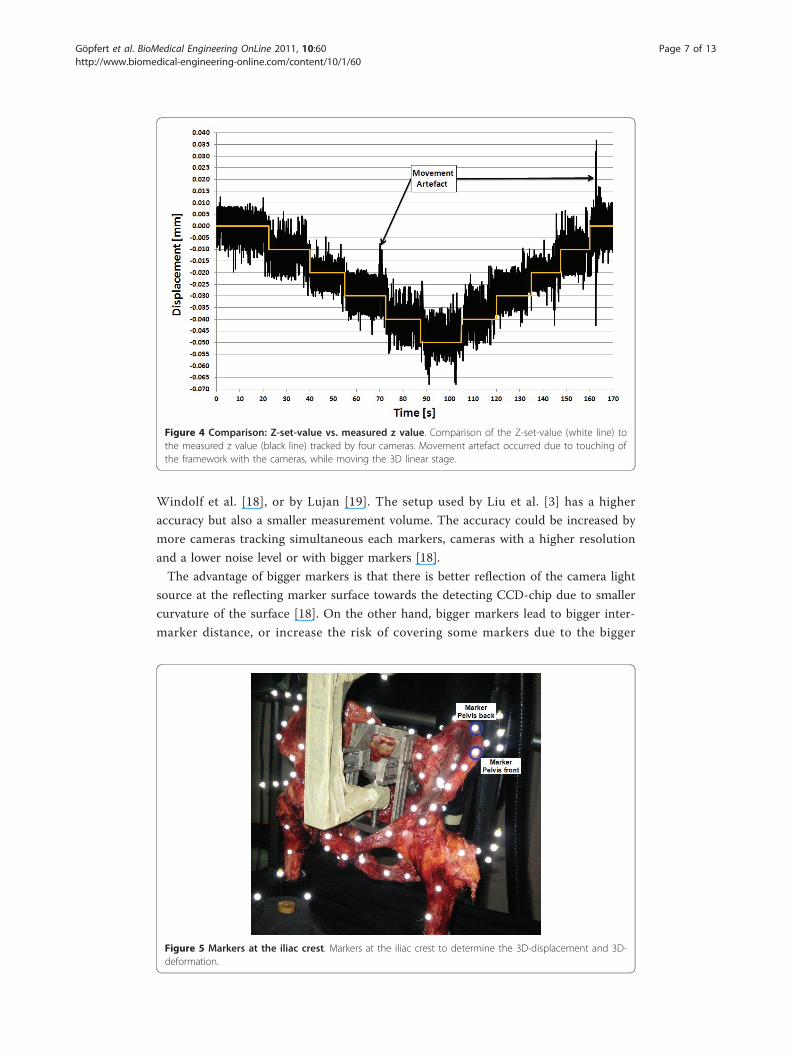
At the iliac crest (Figure 5), the total 3D-displacement between a load of 100N and

900N for the pelvis front marker at the 10th and 90th cycles was 11.972 ± 0.036 mm

(Figure 6) and 13.971 ± 0.036 mm (Figure 7), respectively. The total displacement of

the pelvis back marker was a little bit bigger with 14.188 ± 0.036 mm and 16.294 ±

0.036 mm at the 10th and 90th cycles, respectively for the same loading condition. The

3D-deformation of the iliac crest for the 10th and 90th cycle was 2.146 ± 0.072 mm

and 2.325 ± 0.072 mm, respectively. The difference of the deformation between the

two loading cycles was 0.179 ± 0.072 mm (Figure 8).

The 3D-displacement for the selected marker at the acetabulum (Figure 9) over a

loading cycle at the 10th and 90th cycles was 7.055 ± 0.036 mm (Figure 10) and 8.255

± 0.036 mm (Figure 11), respectively. The 3D-displacement at the femur was much

smaller; being 1.402 ± 0.036 mm and 1.730 ± 0.036 mm at the 10th and 90th cycles,

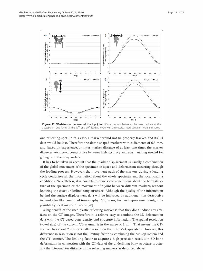
respectively. The 3D-distance change between the two markers across the hip joint at

the 10th and the 90th cycle was 5.656 ± 0.072 mm and 6.526 ± 0.072 mm, respectively.

The difference in the 3D-distance change between the two loading cycles was 0.871 ±

0.072 mm (Figure 12).

DiscussionThe chosen system, combining 3D-video MoCap with servo-hydraulic material testing,

allows dynamic 3D-displacement measurement of the reflecting markers placed on the

surface of a specimen in the sub millimetre range. The accuracy of the measurable

marker displacement with a 3D video MoCap system depends on the number of cam-

eras tracking a single marker simultaneously, on the size and shape of the markers,

and the quality of the camera (CCD-Chip, objective, camera fixation). The accuracy of

± 0.036 mm reached with the setup used in this study is in the range published by

Table 1 Accuracy of the measurement setup depending on the number of camerastracking a marker

Marker visible by n cameras 2 3 6 10 10 static

Noise level [+/- mm] at 0.01 mm step procedure 0.036 0.029 0.021 0.021 0.020

Noise level [+/- mm] at 0.1 mm step procedure 0.035 0.031 0.022 0.018 0.016

Göpfert et al. BioMedical Engineering OnLine 2011, 10:60http://www.biomedical-engineering-online.com/content/10/1/60

Page 6 of 13

Windolf et al. [18], or by Lujan [19]. The setup used by Liu et al. [3] has a higher

accuracy but also a smaller measurement volume. The accuracy could be increased by

more cameras tracking simultaneous each markers, cameras with a higher resolution

and a lower noise level or with bigger markers [18].

The advantage of bigger markers is that there is better reflection of the camera light

source at the reflecting marker surface towards the detecting CCD-chip due to smaller

curvature of the surface [18]. On the other hand, bigger markers lead to bigger inter-

marker distance, or increase the risk of covering some markers due to the bigger

Figure 4 Comparison: Z-set-value vs. measured z value. Comparison of the Z-set-value (white line) tothe measured z value (black line) tracked by four cameras. Movement artefact occurred due to touching ofthe framework with the cameras, while moving the 3D linear stage.

Figure 5 Markers at the iliac crest. Markers at the iliac crest to determine the 3D-displacement and 3D-deformation.

Göpfert et al. BioMedical Engineering OnLine 2011, 10:60http://www.biomedical-engineering-online.com/content/10/1/60

Page 7 of 13

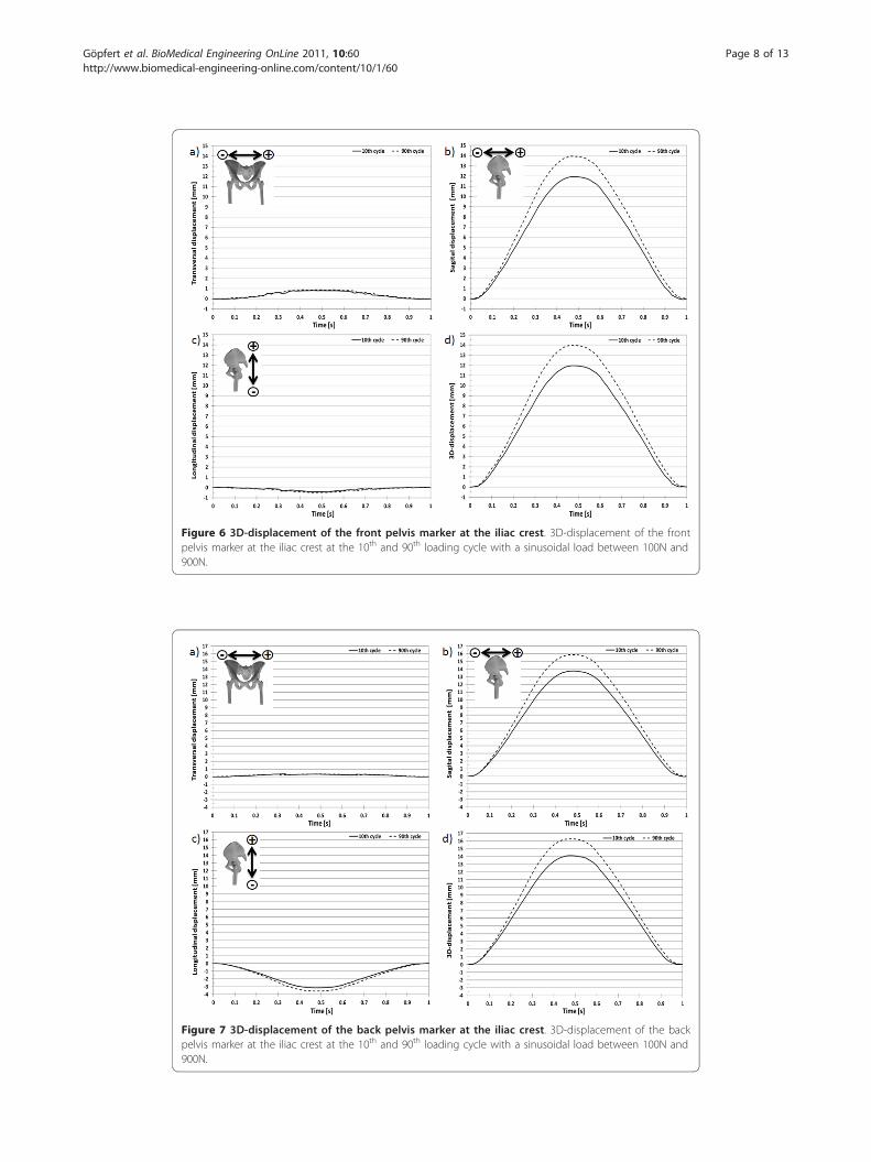
Figure 6 3D-displacement of the front pelvis marker at the iliac crest. 3D-displacement of the frontpelvis marker at the iliac crest at the 10th and 90th loading cycle with a sinusoidal load between 100N and900N.

Figure 7 3D-displacement of the back pelvis marker at the iliac crest. 3D-displacement of the backpelvis marker at the iliac crest at the 10th and 90th loading cycle with a sinusoidal load between 100N and900N.

Göpfert et al. BioMedical Engineering OnLine 2011, 10:60http://www.biomedical-engineering-online.com/content/10/1/60

Page 8 of 13

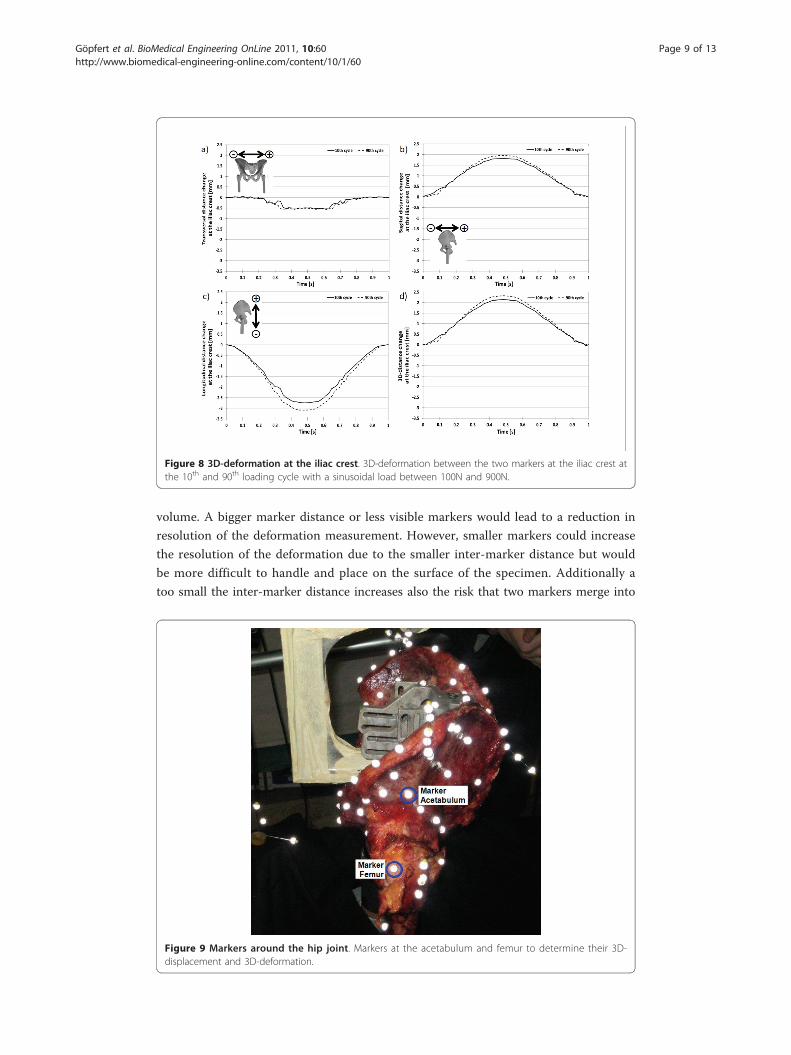
volume. A bigger marker distance or less visible markers would lead to a reduction in

resolution of the deformation measurement. However, smaller markers could increase

the resolution of the deformation due to the smaller inter-marker distance but would

be more difficult to handle and place on the surface of the specimen. Additionally a

too small the inter-marker distance increases also the risk that two markers merge into

Figure 8 3D-deformation at the iliac crest. 3D-deformation between the two markers at the iliac crest atthe 10th and 90th loading cycle with a sinusoidal load between 100N and 900N.

Figure 9 Markers around the hip joint. Markers at the acetabulum and femur to determine their 3D-displacement and 3D-deformation.

Göpfert et al. BioMedical Engineering OnLine 2011, 10:60http://www.biomedical-engineering-online.com/content/10/1/60

Page 9 of 13

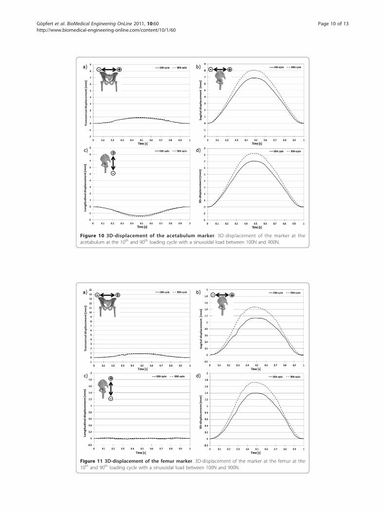
Figure 10 3D-displacement of the acetabulum marker. 3D-displacement of the marker at theacetabulum at the 10th and 90th loading cycle with a sinusoidal load between 100N and 900N.

Figure 11 3D-displacement of the femur marker. 3D-displacement of the marker at the femur at the10th and 90th loading cycle with a sinusoidal load between 100N and 900N.

Göpfert et al. BioMedical Engineering OnLine 2011, 10:60http://www.biomedical-engineering-online.com/content/10/1/60

Page 10 of 13

one reflecting spot. In this case, a marker would not be properly tracked and its 3D

data would be lost. Therefore the dome-shaped markers with a diameter of 6.5 mm,

and, based on experience, an inter-marker distance of at least two times the marker

diameter are a good compromise between high accuracy and easy handling needed for

gluing onto the bony surface.

It has to be taken in account that the marker displacement is usually a combination

of the global movement of the specimen in space and deformation occurring through

the loading process. However, the movement path of the markers during a loading

cycle comprises all the information about the whole specimen and the local loading

conditions. Nevertheless, it is possible to draw some conclusions about the bony struc-

ture of the specimen or the movement of a joint between different markers, without

knowing the exact underline bony structure. Although the quality of the information

behind the surface displacement data will be improved by additional non-destructive

technologies like computed tomography (CT) scans, further improvements might be

possible by local micro-CT scans [20].

A big benefit of the used plastic reflecting marker is that they don’t induce any arti-

facts on the CT-images. Therefore it is relative easy to combine the 3D-deformation

data with the CT-based bone-density and structure information. The spatial resolution

(voxel size) of the current CT-scanner is in the range of 1 mm. That means the CT-

scanner has about 20-times smaller resolution than the MoCap-system. However, this

difference in resolution is not the limiting factor by combining the MoCap-system and

the CT-scanner. The limiting factor to acquire a high precision resolution 3D bone

deformation in connection with the CT-data of the underlining bony structure is actu-

ally the inter-marker distance of the reflecting markers as described above.

Figure 12 3D-deformation around the hip joint. 3D-movement between the two markers at theacetabulum and femur at the 10th and 90th loading cycle with a sinusoidal load between 100N and 900N.

Göpfert et al. BioMedical Engineering OnLine 2011, 10:60http://www.biomedical-engineering-online.com/content/10/1/60

Page 11 of 13

ConclusionsThe combination of 3D video MoCap, and material testing opens new possibilities in

dynamic testing. Combined with CT-data of the underlining bony structure, it becomes

highly valuable framework for finite element modelling of complex implants [13]. It

may also improve the development process of new implant technologies through better

biomechanical compatibility with the patient specific musculoskeletal anatomy.

Acknowledgements and FundingThis project was support by a grant from the ENDO-Stiftung, Hamburg, Germany. We thank Cora Huber, CorinaNüesch, Sarah Schelldorfer, and Dieter Wirz for their help during the measurements.

Author details1Laboratory of Biomechanics & Biocalorimetry, CM&BE, University of Basel, c/o Bio/Pharmazentrum, Klingelbergstrasse50-70, 4056 Basel, Switzerland. 2Paediatric Orthopaedic Department, Children’s University Hospital Basel (UKBB)Spitalstrasse 33, 4056 Basel, Switzerland. 3Laboratory for Movement Analysis Basel, Children’s University Hospital Basel(UKBB), Spitalstrasse 33, 4056 Basel, Switzerland.

Authors’ contributionsAHK, ZK and BG planned the study, BG and MF analyzed the data, AHK and BG wrote the first draft of the manuscript.AHK, MF, ZK and BG took care of revisions. BG, ZK and AHK contributed to interpretation of the results and writing ofthe manuscript. All authors have read and approved the final manuscript.

Competing interestsThe authors declare that they have no competing interests.

Received: 19 January 2011 Accepted: 17 July 2011 Published: 17 July 2011

References1. Blake R, Ferguson H: The motion analysis system for dynamic gait analysis. Clinics in podiatric medicine and surgery

1993, 10-3:501.2. Windolf M, Klos K, Wähnert D, Van Der Pol B, Radtke R, Schwieger K, Jakob R: Biomechanical investigation of an

alternative concept to angular stable plating using conventional fixation hardware. BMC Musculoskeletal Disorders2010, 11-1:95.

3. Liu H, Holt C, Evans S: Accuracy and repeatability of an optical motion analysis system for measuring smalldeformations of biological tissues. J Biomech 2007, 40-1:210-4.

4. Hirokawa S, Yamamoto K, Kawada T: Circumferential measurement and analysis of strain distribution in the humanACL using a photoelastic coating method. Journal of biomechanics 2001, 34-9:1135.

5. Green T, Allvey J, Adams M: Spondylolysis: bending of the inferior articular processes of lumbar vertebrae duringsimulated spinal movements. Spine 1994, 19-23:2683.

6. Häggman Henrikson B, Eriksson P, Nordh E, Zafar H: Evaluation of skin versus teeth attached markers in wirelessoptoelectronic recordings of chewing movements in man. Journal of oral rehabilitation 1998, 25-7:527-34.

7. Kienapfel H, Sprey C, Wilke A, Griss P: Implant fixation by bone ingrowth. The Journal of arthroplasty 1999, 14-3:355-68.8. Tarala M, Janssen D, Telka A, Waanders D, Verdonschot N: Experimental versus computational analysis of

micromotions at the implant-bone interface. Proceedings of the Institution of Mechanical Engineers, Part H: Journal ofEngineering in Medicine 2010, 224:1-8.

9. Widmer K, Wu J, Zurfluh B, Gopfert B, Morscher E: Three-dimensional secondary stability of cemented and non-cemented acetabular implants ex-vivo under dynamic load. Journal of biomechanics 1998, 31-1001:166.

10. Roach P, Eglin D, Rohde K, Perry C: Modern biomaterials: a review–bulk properties and implications of surfacemodifications. Journal of Materials Science: Materials in Medicine 2007, 18-7:1263-77.

11. Currey J: Bone strength: What are we trying to measure? Calcified Tissue International 2001, 68-4:205-10.12. Henninger H, Reese S, Anderson A, Weiss J: Validation of computational models in biomechanics. Proceedings of the

Institution of Mechanical Engineers, Part H: Journal of Engineering in Medicine 2010, 224-7:801-12.13. Cristofolini L, Schileo E, Juszczyk M, Taddei F, Martelli S, Viceconti M: Mechanical testing of bones: the positive

synergy of finite-element models and in vitro experiments. Philosophical Transactions of the Royal Society A:Mathematical, Physical and Engineering Sciences 2010, 368-1920:2725.

14. Gray H, Zavatsky A, Taddei F, Cristofolini L, Gill H: Experimental validation of a finite element model of a compositetibia. Proceedings of the Institution of Mechanical Engineers, Part H: Journal of Engineering in Medicine 2007, 221-3:315-24.

15. Anderson A, Peters C, Tuttle B, Weiss J: Subject-specific finite element model of the pelvis: development, validationand sensitivity studies. Journal of Biomechanical Engineering 2005, 127:364.

16. Abdul-Kadir M, Hansen U, Klabunde R, Lucas D, Amis A: Finite element modelling of primary hip stem stability: Theeffect of interference fit. Journal of biomechanics 2008, 41-3:587-94.

17. Widmer KH, Zurfluh B, Morscher EW: Contact surface and pressure load at implant-bone interface in press-fit cupscompared to natural hip joints. Orthopade 1997, 26-2:181-9.

18. Windolf M, Gotzen N, Morlock M: Systematic accuracy and precision analysis of video motion capturing systems–exemplified on the Vicon-460 system. J Biomech 2008, 41-12:2776-80.

19. Lujan TJ, Lake SP, Plaizier TA, Ellis BJ, Weiss JA: Simultaneous measurement of three-dimensional joint kinematicsand ligament strains with optical methods. J Biomech Eng 2005, 127-1:193-97.

Göpfert et al. BioMedical Engineering OnLine 2011, 10:60http://www.biomedical-engineering-online.com/content/10/1/60

Page 12 of 13

20. Rho J, Hobatho M, Ashman R: Relations of mechanical properties to density and CT numbers in human bone.Medical Engineering & Physics 1995, 17-5:347-55.

doi:10.1186/1475-925X-10-60Cite this article as: Göpfert et al.: 3D video-based deformation measurement of the pelvis bone under dynamiccyclic loading. BioMedical Engineering OnLine 2011 10:60.

Submit your next manuscript to BioMed Centraland take full advantage of:

• Convenient online submission

• Thorough peer review

• No space constraints or color figure charges

• Immediate publication on acceptance

• Inclusion in PubMed, CAS, Scopus and Google Scholar

• Research which is freely available for redistribution

Submit your manuscript at www.biomedcentral.com/submit

Göpfert et al. BioMedical Engineering OnLine 2011, 10:60http://www.biomedical-engineering-online.com/content/10/1/60

Page 13 of 13