3D THERMAL MODEL AND EXPERIMENTAL VALIDATION ...

1

3D THERMAL MODEL AND EXPERIMENTAL VALIDATION OF A LOW VOLTAGE THREE-PHASE BUSDUCT

F.Delgado, C.J.Renedo, A.Ortiz, I. Fernández, A. Santisteban Dept. Electrical and Energy Engineering (ETSII)

University of Cantabria Santander, Spain

e-mail: [email protected] Abstract The thermal behavior of an industrial Low Voltage non-segregated three-phase busduct was analyzed by means of the comparison of a 3D numerical model with experimental results. This model has been carried out using COMSOL Multiphysics, software based on finite element method. The numerical model replicates the short-circuit test, using the same geometry configuration and the boundary conditions of the laboratory in which this assay was carried out. The standard IEC 61439 was applied, both in test and model, in order to obtain the steady state temperatures in several parts of the busbar system. As a result of the data comparison can be concluded that the experimental test was replicated by the numerical model with sufficient accuracy. The temperature differences between simulation results and those of the heating tests were in a narrow range. On the other hand, a sensitivity analysis was carried out with the intention to study the influence of sensors positioning on the temperature measurement in the laboratory test, thus concluding no high precision was needed in the location of the temperature meters. As a final conclusion of this study, it is needed to point out that the numerical model has the enough exactness to be used in the first steps of the busbar design. Keywords Busbar Trunking System (BTS), busway, busduct, 3D Thermal modelling, Numerical Simulation, Experimental validation.

b r o u g h t t o y o u b y C O R EV i e w m e t a d a t a , c i t a t i o n a n d s i m i l a r p a p e r s a t c o r e . a c . u k

p r o v i d e d b y U C r e a

2

Nomenclature Symbols Cp specific heat capacity (J/kg·K) G irradiation (W/m2) h convective heat transfer coefficient (W/m2·K) I rated current (A) k thermal conductivity (W/m·K) L length (m) n normal vector P power losses (W) Q heat production (W/m3) q heat flux by conduction (W/m2) R electrical resistance (Ω) r electrical resistance per unit of length (Ω/m) S section (m2) T temperature (K) Tti tightening torque (N·m) u velocity vector (m/s) V volume (m3) yp proximity effect factor ys skin effect factor Subscribs ac alternate current contact joint Cu copper (conductor) dc direct current F fluid Joule Joule effect S surface Greek letters Nabla operator ε emissivity ρ material density (kg/m3) ρe,20ºC resistivity of copper at 20ºC σ Stefan-Boltzmann constant (W/m2·K4) α coefficient of the resistivity variation with temperature (K-1)

3

1. Introduction An electric Busbar Trunking System (BTS) is an enclosed electrical distribution system comprising solid conductors separated by insulating materials. They are used in many electrical applications due to their technical advantages and cost effectiveness. For instance, the most common use is in the power distribution in a predetermined area, thus feeding applications such as light fittings, factories, offices, etc. Even more, they can be also used in the interconnection between switchboards or between switchboards and transformers.

Many technical specifications have to be fulfilled in these assemblies. Their design is habitually done according the Standard [1], in which many technical requirements are established. Many and very expensive laboratory tests have to be carried out in order to verify that these requirements are fulfilled.

As a consequence of the above, an adequate theoretical design would be needed. This would allow to minimize as much as possible the number of verification tests. The numerical modeling, jointly with the great development of the computational resources, both in hardware and software, seems to be a good way to accomplish the aforementioned goal. Many models can be developed. For instance, the temperature-rise test can be replicated by means of a thermal model.

The thermal modeling is basically employed with two objectives: to determine the temperature distribution in an element and/or to know the heat generated or absorbed by it. Many articles can be found in databases in which this technique is applied looking for these objectives. Several types of software are used in these papers. For example, some authors used MATLAB language programming in order to model the thermal equations, [2-3]. Others authors carried out similar work using others general programming languages in the development of genetic algorithms, [4-5]. This methodology allows the authors to consider (or not) all the physical phenomena they want to model but they need to be expertise in heat transfer and in general programming.

In contrast, other authors used software tools that do not require of programming knowledge. For instance, those applications that are based on finite element method, such as ANSYS and COMSOL Multiphysics. In spite of this type of software allows to obtain the two objectives mentioned above, its main goal is usually to ease the design, the optimization or the control of devices or processes. All of the works that are carried out with this kind of tools in last years are looking for these last objectives. For instance, in 2009, ANSYS Fluent was employed by Rodriguez et al. to model the ice cube production by means of a thermoelectric ice-maker [6]. Two years later, the same program was used by Hu et al. with the intention to obtain the thermal model of a battery [7]. ANSYS is also used in [8]. In this work of 2014 the heat losses in a low-voltage switchgear is calculated. Regarding COMSOL Multiphysics, several devices have been modeled with this tool in the same period. For instance, a mathematical model of a lithium ion battery was developed by Long Cai et al. in 2011, in which thermal effects were considered, [9]. Thermal models of electric machines are developed using this software in papers [10-11], in 2010 and 2013 respectively. More recently, in 2015, Lecuna et al. have carried out a thermal-fluid model of a power transformer, [12].

TOUGH2 is other software that allows to model any device, but in contrast with ANSYS y COMSOL Multiphysics, it can only be applied to heat and moisture transfer problems. That is, it is a specific purpose software. Also, it is based in a different spatial discretization method, the integral finite method. This software is used by Li et al. to study numerically and experimentally the performance of U-vertical ground coupled heat exchanger, [13]. Motor-CAD is other specific purpose software. This analytical network software, developed to study the cooling of electrical machines, is used in 2010 by Staton et al. to analyze the thermal models for small induction motors, [14]. More recently, in 2015, Malumbres et al. used this software to study the thermal and hydraulic modeling of an open self-ventilated electrical machine, [15]. As can be seen in the paragraph above, the thermal models of electrical machines and systems are very usual since their operating conditions and lifetime depend on their heat losses. For instance, in relation to electrical cables, several papers in which thermal models are developed have been made in last years. In 1999, the ampacity derating of electric cables in wrapped trays of nuclear power stations are determined by Figueiredo et al., [16]. Heat losses in underground cables were studied by Kovac et al. in [17], De Lieto et al. in [18] and Chatziathanasiou et al. in [19].

4

Two heat sources have to be considered in the numerical models of electrical conductors: Joule losses in themselves and in the joints between them. These losses result in a temperature increase. As a result of this increase, the electrical conductors can be damaged. For that reason, it is necessary to study their cooling. Heat transfer by conduction, convection and radiation are the three physical phenomena that have to be considered in this cooling. To take into account these phenomena in the numerical models, assumptions and simplifications have to be performed in order to avoid high computational times and requirements.

Considering the above-mentioned issues, a thermal model of a low-voltage non-segregated three phase BTS is presented in this article. This model was carried out by using the heat transfer module of COMSOL Multiphysics. The simulation results were validated by comparing them with experimental results obtained from a heating test. The model validity allows to design new low voltage three-phase BTS. New geometries and materials can be checked or the thermal behaviour of the busways can be studied a priori in different operating conditions. This way, more efficient BTSs can be designed, thus reducing their weight and cost.

Section two presents the BTS definition and its classification. The third section shows the geometrical description of the BTS studied. Experimental test is presented in the fourth section. Fifth section introduces the numerical model developed. Simulation results and their comparison with experimental ones are shown in the sixth section. Finally, conclusions are presented in last section.

2. BTS definition and its classification

According to [20], a BTS can be defined as a type-tested assembly in the form of a conductor system comprising busbars which are spaced and supported by insulating material in a duct, trough or similar enclosure.

In relation to their classification, many criteria can be used to carry out this labour [20]. For instance, according the voltage level, they can be classified in Low Voltage (V1 kV) and High Voltage (V>1 kV) assemblies. Other classification can be obtained with the phase distribution criterion:

o Nonsegregated-phase bus (all phase conductors are in a common enclosure without barriers between the phases, Figures 1.a, 1.b and 1.c.).

o Segregated-phase bus (all phase conductors are in a common enclosure but are segregated by metal barriers between phases).

o Isolated-phase bus (each phase conductor is enclosed by an individual housing separated from the adjacent conductor housing by an air space, Figure 1.d).

If the enclosure is considered, two criteria can be applied. The first of them considers the conductivity of the enclosure: Non-electrical conductive (insulating material with high dielectric strength, Figures 1.a and 1.b) or Metal-enclosed (Figure 1.c.). The second criterion that can be considered is the cooling type applied to the enclosure: Non-ventilated enclosure (an enclosure so constructed as to provide no intentional circulation of external air through the enclosure, Figures 1.a, 1.b and 1.c.), and ventilated enclosure (an enclosure provided with means to permit circulation of sufficient air to remove an excess of heat, fumes, or vapours, Figure 1.d).

5

Figure 1.a. Non segregated-phase Figure 1.b. Non segregated-phase with two

protection conductors

Figure 1.c. Non segregated-phase with metal enclosure

Figure 1.d. Isolated-phase bus with two conductors per phase

Figure 1. Several examples of busbar trunking systems

3. Geometrical description of the BTS studied

As mentioned above, a low voltage non-segregated three-phase busbar system was analyzed in this paper. This busway was designed considering an operating voltage smaller than 1 kV (or equal) and a rated current of 1.5 kA. It is made up six copper bars with two different sections: the larger sections belong to the three phases and the ground, while the two smaller ones belong to the protective conductors. Main dimensions of the studied busway are shown in Figures 2 and 3.

Figure 2.a. Straight lenght Figure 2.b. Joint among straight lengths

Figure 2. Busduct dimensions (mm)

6

Figure 3. Geometrical description of the tested BST (mm)

Different methods can be used to carry out the connection of the straight parts in a busbar. For instance, plates and screws were first used (Figure 4.a). Nowadays, monoblock connections are usually done (Figure 4.b). Applying the correct torque to the screws on these connections allows ensure electrical continuity with a minimum voltage drop.

Figure 4.a. Traditional (with plates and screws) Figure 4.b. Monoblock (with plates and a screw)

Figure 4. Types of Joint pieces

4. Laboratory test

This section is divided in two subsections: test requirements and description test.

4.1. Test requirements

The performance of a BTS is fixed by means of the compliance of the International Standard IEC 61439-6 [1]. Many electrical, mechanical and fire-safety requirements are established by this Standard. The temperature rises of the different components of the BTSs with respect to ambient temperature is one of these requirements. The limits of these temperature rises are prescribed in other part of the Standard, IEC 61439-1, [20]. The verification of these limits can be carried out using several methods. For instance, it can be verified by means of a laboratory test with current, or it can be deduced from the design rules, or it can be calculated using some algebraic method.

In relation to the laboratory test, the climatic chamber have to fulfill several requirements. For instance, its ambient temperature must be among 10ºC and 40ºC, and its average value referred to a 24 hours’ period shall not exceed 35ºC during this test. Also, this chamber must not have forced airflow.

After satisfying the ambient conditions of the laboratory, the previously mentioned temperature limits in the different components of busway must not be exceeded during the temperature-rise

7

test. In this case, the maximum temperature rise is 40ºC for the accessible external enclosure and 105ºC for bare copper busbars.

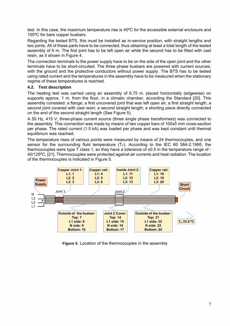
Regarding the tested BTS, this must be installed as in-service position, with straight lengths and two joints. All of these parts have to be connected, thus obtaining at least a total length of the tested assembly of 6 m. The first joint has to be left open air while the second has to be filled with cast resin, as it shown in Figure 4.

The connection terminals to the power supply have to be on the side of the open joint and the other terminals have to be short-circuited. The three phase busbars are powered with current sources, with the ground and the protective conductors without power supply. The BTS has to be tested using rated current and the temperatures in the assembly have to be measured when the stationary regime of these temperatures is reached.

4.2. Test description

The heating test was carried using an assembly of 6.75 m. placed horizontally (edgewise) on supports approx. 1 m. from the floor, in a climatic chamber, according the Standard [20]. This assembly consisted: a flange; a first uncovered joint that was left open air; a first straight length; a second joint covered with cast resin; a second straight length; a shorting piece directly connected on the end of the second straight length (See Figure 5).

A 50 Hz, 415 V, three-phase current source (three single phase transformers) was connected to the assembly. This connection was made by means of two copper bars of 100x5 mm cross-section per phase. The rated current (1.5 kA) was loaded per phase and was kept constant until thermal equilibrium was reached.

The temperature rises of various points were measured by means of 24 thermocouples, and one sensor for the surrounding fluid temperature (TF). According to the IEC 60 584-2:1995, the thermocouples were type T class 1, so they have a tolerance of ±0.5 in the temperature range of -40/125ºC, [21]. Thermocouples were protected against air currents and heat radiation. The location of the thermocouples is indicated in Figure 5.

Figure 5. Location of the thermocouples in the assembly

8

5. Numerical model

This section presents the governing equations and its boundary and initial conditions, the computational domain and its mesh, and the material properties that were used in the numerical model. This was solved considering stationary regime.

5.1. Governing equations

This study was based on the numerical solution of the heat transfer equations, Eqs. (1) and (2).

T ∙ (1)

k (2)

where is the material density, Cp is the specific heat capacity and k is the thermal conductivity. Also, u, is the velocity vector. Moreover, q and Q are the heat flux by conduction and the heat production, respectively.

5.2. Boundary and initial conditions

Two uniform volumetric heat sources were considered: one of them was applied on the straight lengths and the other on the joints. This disparity is due to the different electrical resistance (R) of both parts as a consequence of the contact resistance (Rcontact) that only appears in the aforementioned joints. Subsection 5.4 shows how to calculate the Rs of both parts.

In order to obtain the two heat sources, the Joule losses (PJoule) were determined in both parts of the assembly by using the Eq. (3), in which it was used the rated current (I, 1.5 kA) and the Rs. Obviously, more heat is produced in the connection area than in the rest of the joint piece. However, the high thermal conductivity of copper leads to obtain a similar temperature in this part of the assembly [22]. This way, in first approximation, the heat produced in the connection area can be considered as distributed homogeneously in all the joint piece. This assumption allowed to diminish the computational requirements. Moreover, the experimental results showed that this supposition has sufficient accuracy.

Finally, Q are calculated using Eq. (4), where V is the volume of the parts.

P ∙

(3)

QPV

(4)

Inside the copper the term of the left part of the Eq. (1) is zero since velocity vector has zero value. So, all of the generated heat in the copper is evacuated to the outer surfaces by conduction and the Eq. (1) can be rewritten as Eq. (5).

∙ k (5)

The surfaces of the electrical connection flange were considered as adiabatic areas in order to replicate the heating test in which this flange was covered with a thermal insulated coating of 20 cm width (foam). This boundary condition can be expressed by means of the Eq. (6) that is obtained from Eq. (2) with the right part of the expression equal to zero.

∙ 0 (6)

Heat generated within the assembly flows by conduction to the outer walls, and is emitted outside by convection and radiation, Eq. (7). In this equation, h is the convective heat transfer coefficient, is the emissivity, G is the irradiation (the radiation flux incident on a surface from all directions) and is the Stefan–Boltzmann constant. Finally, TF and Ts are the surrounding fluid temperature and surface temperature, respectively.

9

∙ ∙ ∙ ∙ 7

The convective heat transfer coefficient was calculated depending on the orientation of the surface: vertical wall, horizontal plate upside and horizontal plate downside, [23]. The air temperature in the climatic chamber was 33.9ºC. This temperature has been considered both in the surrounding of the enclosure surfaces and in the space between bars. The two previous approximations have been validated by the experimental results.

Surface-to-ambient radiation has been also considered. The radiative surfaces are the same than those used in convective heat transfer. The insulating surfaces have much higher emissivity than that of the copper (See Table 3 in subsection 5.5).

The above physical model has been solved via “Heat Transfer in solids” interface of the commercial finite elements-based software COMSOL Multiphysics v5.0. This interface allows to combine the heat transfer by conduction, convection and radiation.

5.3. Computational domain and mesh

The 3D entire assembly used in the heating test has been drawn in order to validate the simulation results with those obtained in the experimental test.

The solid parts of the geometry and the air between copper plates in non-insulated joint were considered as computational domain. This was done with the intention to calculate the temperature distribution in the entire model.

Three different free tetrahedral meshing densities were studied: 1.2/2.5/4.6 millions of elements with a quality of 0.64/0.7/0.73, respectively. Similar solutions have been obtained in the three cases. In this paper, among these configurations, the largest meshing density model was selected in order to obtain the most accurate solution, as can be seen in Figure 6.

Figure 6. Computational mesh of the solid domains in the insulating joint

The solution of simulations was reached between 40 and 60 minutes using a workstation with two processors (6 cores/processor) at 2.66 GHz and 48 Gbytes of RAM with a convergence criterion of 10-4 for the residuals values.

5.4. Calculation of the electrical resistances

As mentioned in subsection 5.2, it is needed to calculate the Rs in both parts of the bustduct in order to obtain their heating losses. According the classical theory, in alternate current (a.c.), the RCu was calculated using the Eq. (8).

(8)

10

where rac is the resistance per unit of length and L is the length of the conductor.

At the same time, rac is the sum of the resistance of direct current (rdc) of the conductor plus the skin effect resistance (ysrdc) and the proximity effect resistance (yprdc). The last two resistances only appear in a.c. This can be expressed by means of the Eq. (9) in which ys (skin effect factor) and yp (proximity effect factor) depict both effects.

1 (9)

The proximity effect can be considered negligible (yp0) since the phase conductors are far enough separated so that the magnetic field of each conductor does not affect the current densities of the remaining ones. In the other hand, according [24], the value of the skin effect factor is 0.093.

Regarding the value of rdc, this can be calculated using the Eq. (10), in which S is the section of the conductor, L is the unit length of this conductor and is the resistivity of the copper at 20ºC. This way, the value of rdc at 20ºC (rdc,20ºC) was determined. Nonetheless, the resistivity depends on the operating temperature and in this case the temperatures are close to 85ºC. For that reason, it is necessary to extrapolate rdc,20ºC to the new temperature by using the Eq. (11) in which is the coefficient of the resistivity variation with temperature. In the case of copper, this coefficient is 0.00393.

, ° , ° 1.71 101

0.12 0.00623.75 μΩ (10)

, ,20° 1 – 20

23.75 1 0.00393 85– 20 29.82 μΩ (11)

As a result of the above, and according with Eq. (9), the value of rac is 32.6 /m.

On the other hand, in the joints, apart from the resistance calculated above, there is an additional one, the contact resistance (Rcontact). This mainly depends on the tightening torque (TTi) of the screws. For that reason, Rcontact were measured experimentally for several tightening torques (See Table nº1) in one of the joint of the assembly.

Table 1. Contact resistances vs. tightening torques

TTi (Nm) 5 15 30 45 60

Rcontact (μ) 13 7 4 3 3

In this case, a tightening torque of 45 Nm was used in the joints. So, the Rcontact associated to this torque is 3 μ.

Finally, the total resistances (RTotal) of both parts, shown in Table 2, were calculated by addition.

Table 2. Total resistances of both parts

Straight lengths Joint

RCu 32.6 5.3 172.78 μ 32.6 0.7 22.82μ

Rcontact - 3μ

RTotal 172.78 μ 25.82μ

5.5. Material properties

The physical properties (, k, Cp , and ), shown in Table 3, of the busway solid materials were assumed constant with temperature, except the electrical resistivity, . The enclosure for strength lengths and joints is an insulating material that is made with a mixture of polymeric resins and aggregates. Dimensions are given in Figs. 2 and 3.

11

Table 3. Physical properties of solid materials

[kg/m3]

k [W/(m K)]

Cp

[J/(kg K)] ,

( m)

(1/K) Copper 8,700 400 385 0.19 1.71 10-8 0.00393 Enclosure 1,930 1.05 1,900 0.89

6. Results and discussions

This section presents a base case in which the numerical model of the reference geometry is validated at nominal power rate. Also, other two cases are shown in subsection Other cases in order to corroborate the validity of the model when some variable is changed. Finally, a sensitivity analysis of the sensors position is carried out with the intention to determine if the temperatures values measured depend on the location of the thermocouples.

6.1. Base case

The temperatures distribution of the assembly in stationary regime is shown in Figure 7 (In the sake of clarity, the BST is shown in two parts). According the temperatures range, higher temperatures can be seen in the joints, especially in the non-insulated one.

Figure 7. Temperatures distribution of the assembly

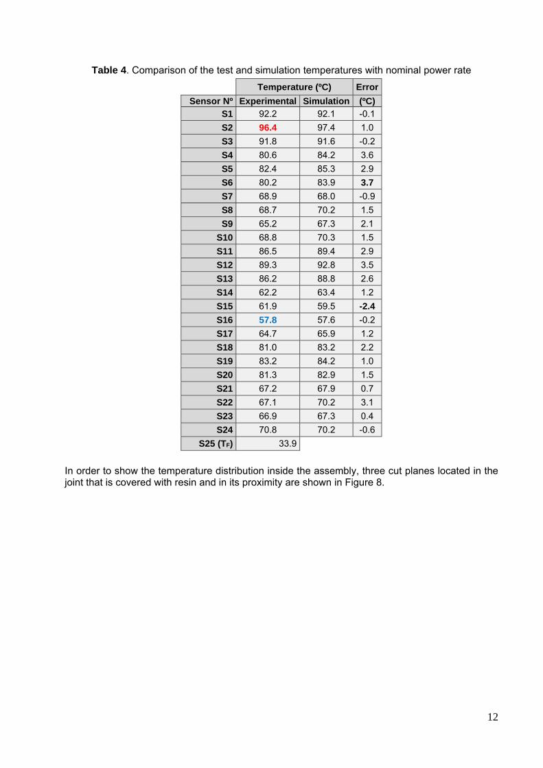
The comparison of the temperature values of the test and the simulation can be seen in Table 4. Also, absolute errors are shown in this table, using test temperature as base value.

According Table 4, the maximum temperature is situated in the inner bar of the joint that is left on air, both in the test and the simulation (sensor 2). On the other hand, the minimum temperature is located in the upper horizontal surface of the joint that is covered with cast resin (sensor 16). Regarding the absolute errors, the differences between both results are in a narrow range, (-2.4+3.7ºC, sensors 15 and 6, respectively).

12

Table 4. Comparison of the test and simulation temperatures with nominal power rate Temperature (ºC) Error

Sensor Nº Experimental Simulation (ºC)

S1 92.2 92.1 -0.1

S2 96.4 97.4 1.0

S3 91.8 91.6 -0.2

S4 80.6 84.2 3.6

S5 82.4 85.3 2.9

S6 80.2 83.9 3.7

S7 68.9 68.0 -0.9

S8 68.7 70.2 1.5

S9 65.2 67.3 2.1

S10 68.8 70.3 1.5

S11 86.5 89.4 2.9

S12 89.3 92.8 3.5

S13 86.2 88.8 2.6

S14 62.2 63.4 1.2

S15 61.9 59.5 -2.4

S16 57.8 57.6 -0.2

S17 64.7 65.9 1.2

S18 81.0 83.2 2.2

S19 83.2 84.2 1.0

S20 81.3 82.9 1.5

S21 67.2 67.9 0.7

S22 67.1 70.2 3.1

S23 66.9 67.3 0.4

S24 70.8 70.2 -0.6

S25 (TF) 33.9

In order to show the temperature distribution inside the assembly, three cut planes located in the joint that is covered with resin and in its proximity are shown in Figure 8.

13

Figure 8a. Cut planes in joint with resin Figure 8b. Joint with resin and straight

lengths Figure 8. Temperatures distribution in the joint with resin and straight lengths

As can be seen in Table 4 and in Figure 8, the highest temperatures are located in the inner bar, decreasing in relation to it with the distance. Also, in spite of a higher heat generation per volume unit of the joint in comparison to the straight lengths due to its Rcontact, its outer insulating surfaces have lower temperatures.

6.2. Other cases

This subsection presents the results of two cases in which some variable of the model has been changed. In the first one, an overload of 20% was applied to the reference geometry. A different BTS geometry was considered in the second one.

6.2.1. Overload case (20%)

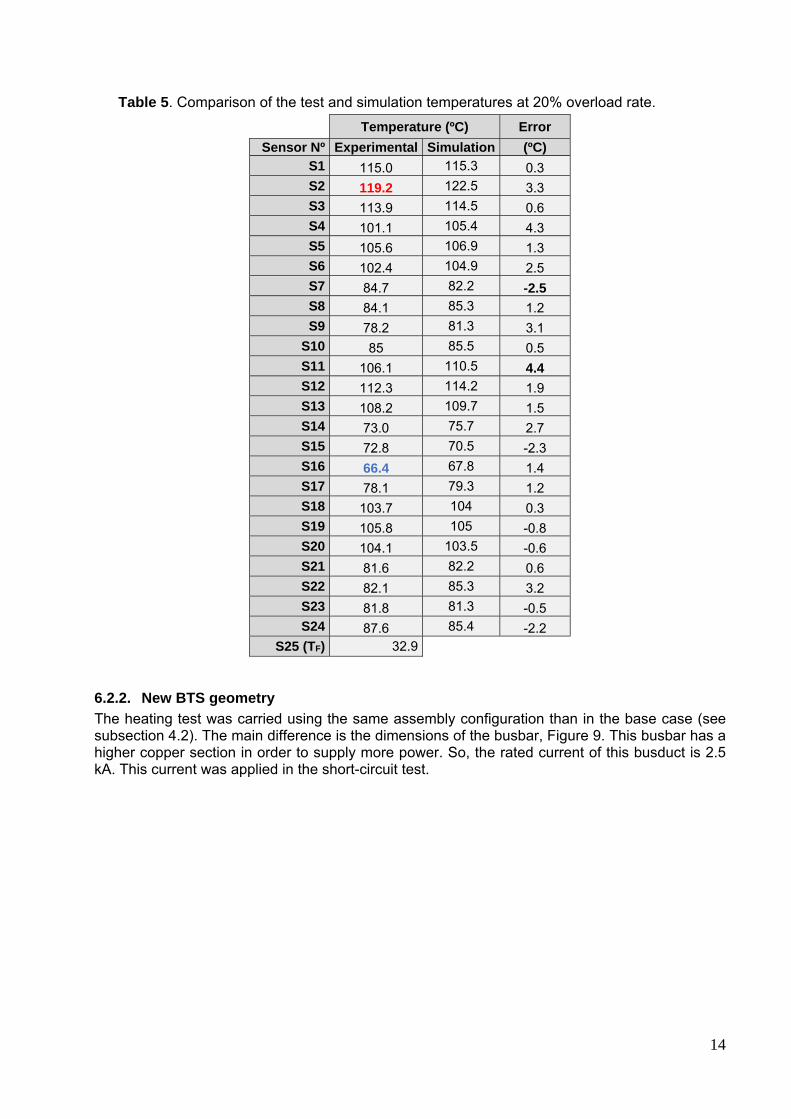
Table 5 shows the comparison of the experimental and simulation data with 1.8 kA (20% overload). The maximum and minimum temperatures are measured with the same sensors than in the base case (S2 and S16). The absolute values of the error are in a range that is slightly higher than the original case (-2.54.4ºC, sensors 7 and 11, respectively).

14

Table 5. Comparison of the test and simulation temperatures at 20% overload rate. Temperature (ºC) Error

Sensor Nº Experimental Simulation (ºC)

S1 115.0 115.3 0.3 S2 119.2 122.5 3.3 S3 113.9 114.5 0.6 S4 101.1 105.4 4.3 S5 105.6 106.9 1.3 S6 102.4 104.9 2.5 S7 84.7 82.2 -2.5S8 84.1 85.3 1.2 S9 78.2 81.3 3.1

S10 85 85.5 0.5 S11 106.1 110.5 4.4 S12 112.3 114.2 1.9 S13 108.2 109.7 1.5 S14 73.0 75.7 2.7 S15 72.8 70.5 -2.3 S16 66.4 67.8 1.4 S17 78.1 79.3 1.2 S18 103.7 104 0.3 S19 105.8 105 -0.8 S20 104.1 103.5 -0.6 S21 81.6 82.2 0.6 S22 82.1 85.3 3.2 S23 81.8 81.3 -0.5 S24 87.6 85.4 -2.2

S25 (TF) 32.9

6.2.2. New BTS geometry

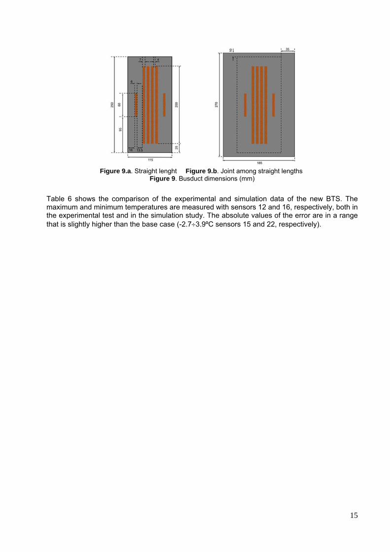
The heating test was carried using the same assembly configuration than in the base case (see subsection 4.2). The main difference is the dimensions of the busbar, Figure 9. This busbar has a higher copper section in order to supply more power. So, the rated current of this busduct is 2.5 kA. This current was applied in the short-circuit test.

15

Figure 9.a. Straight lenght Figure 9.b. Joint among straight lengths

Figure 9. Busduct dimensions (mm)

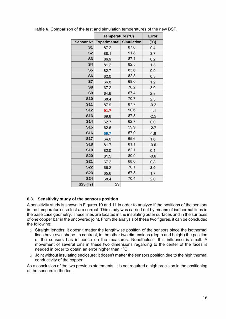
Table 6 shows the comparison of the experimental and simulation data of the new BTS. The maximum and minimum temperatures are measured with sensors 12 and 16, respectively, both in the experimental test and in the simulation study. The absolute values of the error are in a range that is slightly higher than the base case (-2.73.9ºC sensors 15 and 22, respectively).

16

Table 6. Comparison of the test and simulation temperatures of the new BST. Temperature (ºC) Error

Sensor Nº Experimental Simulation (ºC)

S1 87.2 87.6 0.4 S2 88.1 91.8 3.7 S3 86.9 87.1 0.2 S4 81.2 82.5 1.3 S5 82.7 83.6 0.9 S6 82.0 82.3 0.3 S7 66.8 68.0 1.2 S8 67.2 70.2 3.0 S9 64.6 67.4 2.8

S10 68.4 70.7 2.3 S11 87.9 87.7 -0.2 S12 91.7 90.6 -1.1 S13 89.8 87.3 -2.5 S14 62.7 62.7 0.0 S15 62.6 59.9 -2.7 S16 59.7 57.9 -1.8 S17 64.0 65.6 1.6 S18 81.7 81.1 -0.6 S19 82.0 82.1 0.1 S20 81.5 80.9 -0.6 S21 67.2 68.0 0.8 S22 66.2 70.1 3.9 S23 65.6 67.3 1.7 S24 68.4 70.4 2.0

S25 (TF) 29

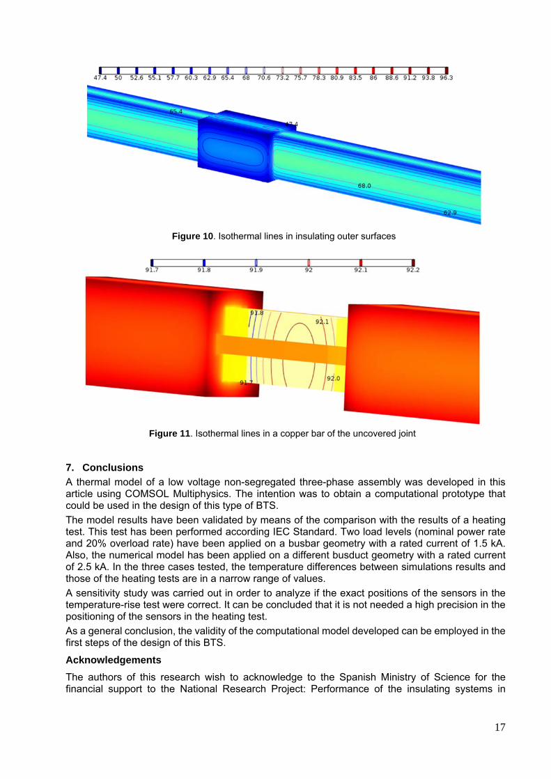
6.3. Sensitivity study of the sensors position

A sensitivity study is shown in Figures 10 and 11 in order to analyze if the positions of the sensors in the temperature-rise test are correct. This study was carried out by means of isothermal lines in the base case geometry. These lines are located in the insulating outer surfaces and in the surfaces of one copper bar in the uncovered joint. From the analysis of these two figures, it can be concluded the following:

o Straight lengths: it doesn't matter the lengthwise position of the sensors since the isothermal lines have oval shape. In contrast, in the other two dimensions (depth and height) the position of the sensors has influence on the measures. Nonetheless, this influence is small. A movement of several cms in these two dimensions regarding to the center of the faces is needed in order to obtain an error higher than 1ºC.

o Joint without insulating enclosure: it doesn’t matter the sensors position due to the high thermal conductivity of the copper.

As a conclusion of the two previous statements, it is not required a high precision in the positioning of the sensors in the test.

17

Figure 10. Isothermal lines in insulating outer surfaces

Figure 11. Isothermal lines in a copper bar of the uncovered joint

7. Conclusions

A thermal model of a low voltage non-segregated three-phase assembly was developed in this article using COMSOL Multiphysics. The intention was to obtain a computational prototype that could be used in the design of this type of BTS.

The model results have been validated by means of the comparison with the results of a heating test. This test has been performed according IEC Standard. Two load levels (nominal power rate and 20% overload rate) have been applied on a busbar geometry with a rated current of 1.5 kA. Also, the numerical model has been applied on a different busduct geometry with a rated current of 2.5 kA. In the three cases tested, the temperature differences between simulations results and those of the heating tests are in a narrow range of values.

A sensitivity study was carried out in order to analyze if the exact positions of the sensors in the temperature-rise test were correct. It can be concluded that it is not needed a high precision in the positioning of the sensors in the heating test.

As a general conclusion, the validity of the computational model developed can be employed in the first steps of the design of this BTS.

Acknowledgements

The authors of this research wish to acknowledge to the Spanish Ministry of Science for the financial support to the National Research Project: Performance of the insulating systems in

18

transformers: alternative dielectrics. thermal-fluid modelling and post-mortem analysis (DPI2013-43897-P).

References

[1] IEC. IEC 61439-6: Low-voltage switchgear and controlgear assemblies - part 6: Busbar trunking systems (busways). 2012).

[2] M. A. Rey-Ronco. T. Alonso-Sánchez. J. Coppen-Rodríguez and M. P. Castro-García. "A thermal model and experimental procedure for a point-source approach to determining the thermal properties of drill cuttings." Journal of Mathematical Chemistry. vol. 51. pp. 1139-1152. 2013.

[3] S. Taheri. A. Gholami. I. Fofana and H. Taheri. "Modeling and simulation of transformer loading capability and hot spot temperature under harmonic conditions." Electr. Power Syst. Res.. vol. 86. pp. 68-75. 2012.

[4] V. Galdi. L. Ippolito. A. Piccolo and A. Vaccaro. "Parameter identification of power transformers thermal model via genetic algorithms." Electr. Power Syst. Res.. vol. 60. pp. 107-113. 2001.

[5] W. H. Tang. Q. H. Wu and Z. J. Richardson. "A simplified transformer thermal model based on thermal-electric analogy." IEEE Trans. Power Del.. vol. 19. pp. 1112-1119. 2004.

[6] A. Rodríguez. J. G. Vián and D. Astrain. "Development and experimental validation of a computational model in order to simulate ice cube production in a thermoelectric ice-maker." Appl. Therm. Eng.. vol. 29. pp. 2961-2969. 2009.

[7] X. Hu. S. Lin. S. Stanton and W. Lian. "A Foster network thermal model for HEV/EV battery modeling." IEEE Trans. Ind. Appl.. vol. 47. pp. 1692-1699. 2011.

[8] M. Bedkowski. J. Smolka. K. Banasiak. Z. Bulinski. A. J. Nowak. T. Tomanek and A. Wajda. "Coupled numerical modelling of power loss generation in busbar system of low-voltage switchgear." International Journal of Thermal Sciences. vol. 82. pp. 122-129. 2014.

[9] L. Cai and R. E. White. "Mathematical modeling of a lithium ion battery with thermal effects in COMSOL Inc. Multiphysics (MP) software." J. Power Sources. vol. 196. pp. 5985-5989. 2011.

[10] T. A. Jankowski. F. C. Prenger. D. D. Hill. S. R. O'Bryan. K. K. Sheth. E. B. Brookbank. D. F. A. Hunt and Y. A. Orrego. "Development and validation of a thermal model for electric induction motors." IEEE Trans. Ind. Electron.. vol. 57. pp. 4043-4054. 2010.

[11] M. Zhang. M. Chudy. W. Wang. Y. Chen. Z. Huang. Z. Zhong. W. Yuan. J. Kvitkovic. S. V. Pamidi and T. A. Coombs. "AC loss estimation of HTS armature windings for electric machines." IEEE Trans. Appl. Supercond.. vol. 23. 2013.

[12] R. Lecuna. F. Delgado. P. Castro. A. Ortiz. I. Fernández and C. J. Renedo. "Thermal-fluid Characterization of Alternative Liquids of Power Transformers: a Numerical Approach." IEEE Transactions on Dielectrics and Electrical Insulation. 10/2015. 2015.

[13] X. Li. Z. Chen and J. Zhao. "Simulation and experiment on the thermal performance of U-vertical ground coupled heat exchanger." Appl. Therm. Eng.. vol. 26. pp. 1564-1571. 2006.

[14] D. Staton and M. Popescu. "Analytical thermal models for small induction motors." COMPEL - the International Journal for Computation and Mathematics in Electrical and Electronic Engineering. vol. 29. pp. 1345-1360. 2010.

[15] J. A. Malumbres. M. Satrustegui. I. Elosegui. J. C. Ramos and M. Martínez-Iturralde. "Analysis of relevant aspects of thermal and hydraulic modeling of electric machines. Application in an Open Self Ventilated machine." Appl. Therm. Eng.. vol. 75. pp. 277-288. 2015.

[16] R. D. C. A. Figueiredo. S. Carneiro Jr. and M. E. C. Cruz. "Experimental validation of a thermal model for the ampacity derating of electric cables in wrapped trays." IEEE Trans. Power Del.. vol. 14. pp. 735-742. 1999.

[17] N. Kovac. I. Sarajcev and D. Poljak. "Nonlinear-coupled electric-thermal modeling of underground cable systems." IEEE Trans. Power Del.. vol. 21. pp. 4-14. 2006.

[18] R. De Lieto Vollaro. L. Fontana and A. Vallati. "Thermal analysis of underground electrical power cables buried in non-homogeneous soils." Appl. Therm. Eng.. vol. 31. pp. 772-778. 2011.

19

[19] V. Chatziathanasiou. P. Chatzipanagiotou. I. Papagiannopoulos. G. De Mey and B. Wiȩcek. "Dynamic thermal analysis of underground medium power cables using thermal impedance. time constant distribution and structure function." Appl. Therm. Eng.. vol. 60. pp. 256-260. 2013.

[20] IEC. IEC 61439-1: Low-voltage switchgear and controlgear assemblies - part 1: General rules. 2012.

[21] IEC. IEC 60 584-2: Thermocouples. Part 2: Tolerances. 1995.

[22] J. Lotiya. "Thermal analysis and optimization of temperature rise in busbar joints configuration by FEM." 6th IEEE Power India International Conference, PIICON 2014, 2014.

[23] COMSOL. Heat transfer module user's guide. COMSOL 5.0. October 2014).

[24] P. Silvester. "AC Resistance and Reactance of Isolated Rectangular Conductors." IEEE Transactions on Power Apparatus and Systems. vol. PAS-86. pp. 770-774. 1967.