3D-Modeling of Long span Bridges and Fluid-Structure ...

Journal of Al Azhar University Engineering Sector

Vol. 12, No. 45, October, 2017, 1267-1284

3D-MODELING OF LONG SPAN BRIDGES AND FLUID-STRUCTURE

INTERACTION DOMAINS

Mohamed O. Elgohary and Walid A. Attia:

Department of structural engineering, Cairo University ABSTRACT

Analysis of long span cable bridge such as: Cable stead or Suspension bridges under the effect of fluid structure interaction (FSI) became the main parameter affect design and safety of long spans bridges. In this research we will discussed, the 3D-CFD Finite element modeling of the wind flows around bridges. The 2D-modeling of the bridge deck and the fluid domain around it to get the critical wind speed without flutter occurs, aren’t more accurse in the bridge modeling. There are many out of plane parameters that affect the critical wind speed and flutter. But also the 3D-Modeling of the bridge and the fluid domain using the finite element theory in all of computer programs are very difficult because it need a huge disk space and long time to run the analysis. Therefore the research studies the reshape of fluid interaction 3D-domain, and How to make it optimum in analysis, time, and efficient results. The optimum 3D-domain takes every in plane and out of plane parameters the affect the long span bridge modeling. That gets accurate nearest simulation to bridge behavior in fluid structure interaction closed to the wind tunnel test. I. INTRODUCTION The design of bridges, in particular long spanned ones, is challenging in the sense that there are many complicated issues to be considered. Amidst the loads to be considered, like dead load, live load, wind load, and earthquake load, the wind load becomes the prime concern for the design of the bridges. Traditionally, analysis of a bridge structure and the wind effects are studied using wind tunnel experiments. This usually takes 6-8 weeks and also it is very costly. With the explosive growth in the electronic and computer industry there has been a tremendous increase in the computing power and speed. Therefore, now the shift is towards computer modeling of the wind induced effects on a bridge structure by using the principles of Computational Structural Dynamics (CSD) and Computational Fluid Dynamics (CFD). This reduces cost and time considerably when compared to the traditional approach of wind tunnel experiments for design and analysis of bridges.

The Tacoma Narrows Bridge at Washington, opened in 1940, is a well-known classical example of a bridge failure due to wind. This bridge had abnormally excessive deflections both during construction and service. A wind velocity as low as 42 mph ripped apart the bridge and tore it, buckling the stiffening girders at the mid span (Bowers, 1940). This failure was due to the phenomenon of flutter.

Flutter occurs if the velocity of wind is higher than the critical velocity for a given bridge. This failure brought awareness to the designers around the world that wind can cause aerodynamic instability of bridges resulting in failure. Thus it becomes necessary and important to conduct sufficient aerodynamic studies of the bridge before construction so that the stability of the bridge against wind can be ensured.

3D-MODELING OF LONG SPAN BRIDGES AND FLUID-STRUCTURE INTERACTION DOMAINS

(a)

(b)

Fig (1) show The collapse of the Tacoma Narrows Bridge, (a) torsional motion led to collapse, (b) separated

vortex descending by flow visualization.

Torsional motion of the bridge superstructure that lead to bridge collapse, and the vertical displacement occurs as shown in Figure (1-1) a ,d. Since this accident, the importance of wind-resistant design for long-span suspension bridges has been highly recognized and has led to many research works and investigations on bridge aerodynamics. Farquharson et al. [2] conducted a series of wind tunnel experiments on the Tacoma Narrows Br. Bleich [3] made analytical studies on the flutter problem. In them they developed the instability analysis using motion-dependent forces on a thin airfoil given by The odorsen [4] in the field of aeronautics. The odorsen’s formulas are written for the form of harmonic motion as

2. Computational bridge aerodynamics review

The need for numerical models is highly desirable because the high Re present at full scale cannot be reproduced in Conventional wind tunnel experiments. Numerical bridge aerodynamics studies are still a young field in computational fluid dynamics research. In the late 1990s a series of publications revealed that significant computational research had begun in this area. In the following, a brief review is given on numerical bridge deck studies. We will learn that the majority of the studies done to model flow around bridge decks numerically include 2-D fluid-only analyses (i.e., flow past stationary decks); both with/without turbulence models. Results from these analyses are typically steady-state coefficients (drag, lift and moment) and Strouhal number. Comprehensive studies have also been carried out on elastically suspended bridge decks which involve analyses with prescribed deck motion allowing linearized aerodynamic motional force coefficients (flutter derivatives) to be determined (Scanlan and Tomko, 1971).


The literature also revealed that numerical bridge flutter models usually are 2D without

attempts to include a turbulence model formulation. Other aero elastic phenomena, for example, buffeting [e.g., Turbelin and Gibert (2002)] and vortex-induced oscillation [e.g., Lee et al.(1995) ] have gotten less attention with regard to computational predictions. We note that this does not necessarily imply they are less important.

The Re is about a factor 10 lower compared to the flow near the flutter limit. As with other bluff bodies, capturing three-dimensional (3-D) effects and turbulence in the free-stream and in flow instability zones play an important role in replicating these phenomena which in turn make them more difficult to model accurately. Dealing with moderate/high Re naturally raises questions with regard to the importance of modeling three-dimensionality and turbulence. However, accurate flutter predictions appear to be mainly affected by the leading edge separations and the associated pressure forces. Further we note, for sharp leading edges, accurate turbulence modeling and 3-D effects may not be important, whereas it could play a strong role for bridge decks with rounded edges.

One of the first numerical bridge deck simulations relate to the finite-difference method (FDM) and was explored by Fujiwara et al.(1993) , both on stationary and moving 2-D grids discredited by 20451 grid points. The Navier–Stokes solutions presented were for Re in the range of 2100 – 4000 following wind tunnel experiments. Onset wind-speed predictions agreed in general with the wind tunnel experiments, but discrepancies were found in the amplitudes, these being overestimated by the numerical model. Fujiwara et al .reported that a possible explanation could be the loss of 3-D effects, the 2-D solution predicting larger fluctuations of lift. Furthermore, Onyemelukwe (1993) developed a 2-D finite difference solver on boundary fitted grids. Laminar Navier–Stokes flow solutions were presented for a variety of fixed bridge decks around Re of 1 _ 105: The comprehensive numerical flow visualization studies of Onyemelukwe (1993) were however suppressed by restrictions in CPU and memory. He reported that static force coefficients could not be computed on his IBM 386 PC. It is interesting to note that 10 years after this is no longer a barrier.

Later Onyemelukwe et al.(1998) reported on SunSPARC10 simulations but those were related to flow around circular cylinders. In the mid-1990s Kuroda (1997) developed a laminar Navier–Stokes solver discredited also based on the FDM. Solutions for a fixed bridge embedded in an O-grid-type discredited flow domain with 221 _ 101 grid points were shown. Pressure distributions on the deck and static coefficients for Re of 3 _ 105 for a range of angle of attacks agreed well with the results of the wind tunnel tests. Comparable studies to the present FE flutter simulations include the work of Jenssen and Kvamsdal (1999), who uses the finite volume method (FVM) to model the flow field on moving unstructured regular grids. Jenssen and Kvamsdal (1999) show results based on parallel computing techniques.

Following the wind tunnel tests and in recognition of inadequate turbulence modeling, the Re was physically incorrect ð0:45 _ 105Þ and was kept constant for all wind velocities. The flutter limit was based on 2-D analyses with prescribed deck motions (as opposed to self-excited motions) which was in good agreement with the flutter limit derived from the wind tunnel tests. In contrast to the fully coupled FSI solutions presented in the present simulations, Jenssen and Kvamsdal have a coupling module included in their numerical approach between the FVM fluid solver and an FE structural solver, which resulted in weakly coupled solutions (as described later in Section 3; also shown in Fig.5 ).A background to staggered transient analysis for coupled mechanical system is described in detail by Felippa and Park (1980).Furthermore, Jenssen and Kvamsdal (1999) are currently one of the few researchers who have done numerical bridge studies on 3-D flow models.Their investigations include large eddy simulations on stationary grids expanding a 2-D model of 75 000 cells to 40 _ 75 000 cells over a distance of 0:2 _ B (where B is the width of the bridge of 31 m) along the span, from which they conclude that the pressure distribution, the steady state lift and pitching moment are in closer agreement with the results of the wind tunnel [see also Jenssen, 1998].However, the present investigations indicate that it does not appear evident that models of this size are required nor that 3-D simulations are


required for the flutter limit prediction as 2D coarse models (E1900 nodes in an irregular unstructured grid) without boundary layer modeling seems sufficient, as shown later in Section 5. Other investigators have also used and developed FVM solvers .For example, De Foy (1998) applied his unsteady incompressible finite volume solver to the Great Belt East bridge deck section. Fluid-only simulations in 2-D were performed for a Re of 1:38 _ 108; assuming laminar flow .De Foy found an St ¼ 0:17 which compares reasonable well with the section model of the wind tunnel (0.11– 0.15), where Re was in the order of 0:4 _ 105 to 1:5 _ 105:

Furthermore, Bruno et al.(2001) applied the FVM which includes a k–e-model when solving the flow past the complicated leading edge detail (including railings) of the Normandy cable-stayed bridge (France).Using parallel computations, Bruno et al.(2001) present 2-D flow results for the stationary bridge deck. Their optimized fluid model consist of an unstructured irregular grid with domain size of 50B _ 40B: The fluid domain is discredited by 29 000 nodes with a cell thickness at the wall of 2 _ 10_3B; where the width of the bridge deck, BE21:2 m: They reported good agreement with the wind tunnel results when comparing force coefficients for the fixed bridge deck. Previous numerical studies using the FE method have been undertaken by, e.g., Lee et al.(1995) , Mendes and Branco (1998) and Selvam et al.(2002) . Lee et al.(1995) modeled FSI through moving structured regular grids adopting the ALE formulation. Their 2-D fluid model included a k–e-model and a streamlined-upwind

Petrov Galerkin (SUPG) approximation was assumed. Lee et al.(1995) explored the use of this FE approach on several bridges.The static force coefficients agreed with the results obtained in the wind tunnel but some discrepancies were found with regard to the onset velocity of vortex-induced resonance. Mendes and Branco (1998) carried out flow investigations on the Vasco da Gama cable-stayed bridge (Portugal).They assumed laminar flow. However in recognition of the high prototype Re, an incorrect low value of Re ð3 _ 103Þ was used in the demonstration of the flow solutions. For this flow regime, their studies demonstrated that a cross-section with baffles aids the suppression of torsional instability. Furthermore, Selvam (1998) developed an FE model on a rotating moving frame of reference. Their FE model was to the approach bridges of the Great Belt East (Denmark) and, in a more recent analysis, to the main suspension bridge (Selvam et al., 2002).

Selvam et al.present large eddy simulations for an Re in the order of 105: In their recent analysis they use structured regular grids of 14 805 nodes contained within a control volume 3B _ 8B: They report on drag coefficients and the flutter instability limit which are in agreement with the wind tunnel tests.

In recent years the spectral method, described by Karniadakis and Sherwin (1999), has made interesting contributions to modelling moving boundaries.A main advantage is resolving the steep boundary layer gradients and shear layers with high-order resolution.Spectral element methods also allow for advecting the flow structures with greater accuracy similar to the vortex methods described below.Using spectral elements also seem to be less CPU demanding compared to the ALE approach. Li et al.(2002) developed and applied their spectral method based on a rotating moving frame of reference.In a 2-D case study, they applied their model to predict the flutter limit of the Second Forth Road Bridge, UK (Robertson et al., 2003b).

The computational irregular unstructured mesh was made up of 1789 elements and Re

ranged between 4167 to 11 667.Good agreement with wind tunnel tests were found although the physical small-scale experiments were based on Re in the order of 1 _ 105 to 1 _ 106:

Futhermore, the spectral method of Li et al.(2002) was also applied to explore the single degree of freedom instability problem of galloping of bluff bodies, e.g.,Robertson et al.(2003a) .Recent investigations provide more detail on bridge deckbehavior, as described by Robertson et al.(2003c) . Grid generation (even in 2-D) can be a time-consuming process, especially when the grids involve bluff bodies. Tothis end, avoiding the use of grids, the discrete-vortex method


(DVM) pioneered in the 1960s by Sarpkaya and Chorin as described in the comprehensive reviews [e.g., Sarpkaya (1989), Chorin (1989)], is attractive for FSI analysis.DVM has been popular for many decades (Leonard, 1980).In particular, the method of source panels has been used for studying aerodynamic interactions among various components of an aircraft.The vortex elements are naturally concentrated into areas of nonzero vorticity and unlike the grid-based methods, this means that the small-scale flow structures will automatically be captured.However, DVM developers are faced with other difficulties in that several parameters must be prescribed, such as the core radius, defining the maximum circulation to be released for one boundary element and at which distance the surface vorticity is to be released from the bridge surface.

The 2-D DVM has been applied to bridge decks by, e.g., Walther (1994), Morgenthal and McRobie (2002), Taylor and Vezza (2002).

In a series of publications, e.g., Walther and Larsen (1997) show flow solutions for fixed bridge decks and flutter limit predictions in agreement with wind tunnel results. Taylor and Vezza (2002) have also developed a DVM solver and present results on stationary and oscillating bridge decks.The derived flutter limit based on prescribed motion compare well with wind tunnel tests.In addition, they show extensive investigations of the flutter motion being suppressed by inclusion of active control vanes. Finally, it should be mentioned that various investigators have used hybrid models.

For example, Brar (1997) developed a coupled finite-difference and vortex-method scheme.An Eulerian finite-difference grid was located in the viscous region next to the bluff body section and the Lagrangian vortex element domain in the flow regions away form the wall boundaries.Flow solutions were presented for Re of 100–1000.St predictions agreed in general with the solutions of others.In some case, the numerical solution overpredicted the St.

This present paper explores the use of a fully coupled FE FSI solver to simulate (1) flow past a fixed deck and (2) to predict the self-excited flutter instability limit.

3. The FE formulation & Turbulence flow The numerical solutions of the convection-dominated flow are obtained from a semi-discrete FE formulation of the flow field equations assuming isothermal incompressible viscous flow contained within the multiphysics FE code Spectrum (Ansys Inc., 1999).A brief theoretical background of Spectrum is presented here and is limited to the context of the application to long-span bridge aeroelasticity.To the knowledge of the author, this is a new application of Spectrum. The most closely related work is the project of Okstad and Mathisen (1998) and Remseth et al.(1999) .They used Spectrum to carry out the FSI simulations for a Reynolds number of 12 812 on a submerged road bridge. They showed results from 2-D simulations of water flow past an elastically suspended circular cross-section.The cylinder displacements agreed quantitatively well with the water-tank experiments reported in Dahle et al.(1990) . Okstad and Mathisen (1998) also concluded that the FSI simulations indicated a larger dependency on the FE mesh than the corresponding fixed cylinder case.Although difficulties in the numerical experiments were experienced, these were mainly due to the free surface behavior, and thus not particularly relevant to the bridge aerodynamic problem.

In this study, investigations into the FSI mechanisms due to wind action on either a stationary or a moving long-span bridge deck are carried out.The FE model of this coupled FSI problem consists of three main regions: (i) the fluid domain where the incompressible Navier–Stokes equations (NSEs) are to be solved; (ii) the structural domain where nonlinear elasticity equations are to be solved; and (iii) the interface region.For this application the mathematical formulation strongly couples the incompressible isothermal Navier–Stokes equations of the fluid to the structural equations. This is achieved by means of an ALE formulation, where the FE mesh is allowed to move independently of the motion of the fluid particles themselves. The


numerical results presented herein are based on 2-D models. For the FE theory however, the third dimension does not complicate the formulation and no such restriction is imposed. CHOOSING TURBULENCE MODEL It is an unfortunate fact that no single turbulence is universally accepted as being superior for all classes of problems. The choice of turbulence model will depend on considerations such as the physics encompassed in the flow, the established practice for a specific class of problem, the level of accuracy required, the available computational resource, and the amount of time available for the simulation. To make the most appropriate choice of model for your application, you need to understand the capabilities and limitations of the various options. Thus we give over view of turbulence models types will depend on the flow type that you are model:

A- Reynolds-Average Approach vs. LES. B- Reynolds Averaging. C- Boussinesq Approach vs. Reynolds Stress Transport Models

A-Reynolds-Average Approach vs. LES. Time-dependent solution of Navier-Stokes equations for high Reynolds-number turbulent flow in complex geometry which set out to resolve all the way down to the smallest scales of the motions are unlikely to be attainable for some time to come. Two alternative methods can be employed to render the Navier-Stokes equations tractable so that the small-scale turbulent fluctuations do not have to be directly simulated; Reynolds-averaging and filtering. Both methods introduce additional terms in the governing equations that need to be modeled in order to achieve “closure” for the unknowns. The Reynolds-averaged Navier stokes (RANS) equations govern the transport of the average flow quantities, with the whole range of the scales of turbulence being modeled. The RANS based modeling approach therefore greatly reduced the required computational effort and resource, and is widely adopted for practical engineering applications. An entire hierarchy of closure is available in ANSYS FLUENT including Spalart-allarams, and its variants, and its variants, and the RSM. The RANS equations are often used to compute time-dependent flows, whose unsteadiness may be externally imposed (e.g., time-dependent boundary conditions or sources) or self-sustained (e.g., vortex-shedding, flow instability). LES provides an alternative approach in which large eddies are explicitly computer (resolved) in a time –dependent simulation using the “filtered “ Navier-Stokes equations. The rationale behind LES is that by modeling less of turbulence (and resolving more), the error introduced by turbulence modeling can be reduced. It is also believed to be easier to find a “universal” model for small scales, since they tend to be more isotropic and less affected by the macroscopic features like boundary conditions, than the large eddies .Filtering is essentially a mathematical manipulation of the exact Navier-Stokes equations to remove the eddies that are smaller than the size of the filter, which is usually taken as the mesh size when spatial filtering is employed as in ANSYS FLUENT. Like Reynolds-averaging, the filtering process creates additional unknowns terns that must be modeled to achieves closure. Statistics of the time-varying flow-field such as time-average and r.m.s. values of the solutions variables, which are generally of most engineering interest, can be collected during the time-dependent simulation. Les for high Reynolds number industrial flow requires significant computational resources. This is mainly because of the need to accurately resolved the energy-containing turbulent eddies in both space and time domains, which becomes most accurate in near wall regions where the scales to become much smaller. Wall functions in combination with a coarse near wall mesh can be employed, often with some success, to reduce the cost of LES for wall-bounded flow. However, one needs to carefully consider the ramification of using wall functions for the flow in question. For the same reason (to accurately resolve the eddies), LES also requires highly accurate special and temporal discretizations.


B-Reynolds (Ensemble) Averaging

In Reynolds averaging, the solution variables in the instantaneous (exact) Naier-Stokes equations

are decomposed into the mean (ensemble-average or time –averaged) and fluctuating

components. For the velocity components:

Where: are the mean and fluctuating velocity components (i =1, 2, 3).

Likewise, for pressure and other scalar quantities:

Where denotes a scalar such as pressure, energy, or species concentration.

Substituting expressions of this for the flow variables into the instantaneous continuity and

momentum equations and taking a time (or ensemble) average (and dropping the overbar on the

mean velocity, ) yields the ensemble-average momentum equations. They can be written in

Cartesian tensor form as:

These two equations are called Reynolds-average Navier-stoke (RANS) equations. They have

the same general form as the instantaneous Navier-Stokes equations, with the velocity and other

solution variables now presenting ensemble-averaged (or time averaged) values. Additional

terms now apper that present the effect of turbulence. These Reynolds stresses , must

be modeled in order to close the second equation .

For variables-density flows, the above tow equations can be interpreted as Favre-averaged

Navier-Stokes equations with the velocity representing mass-averaged values.

C- BOUSSINESQ APPROACH VS. REYNOLDS STRESS TRANSPORT MODELS

The Reynolds-averaged approach to turbulence modeling requires that Reynolds stresses in

Navier equations are appropriately modeled. A common method employs the Boussinesq

hypothesis to relate Reynolds stresses to the mean velocity gradients:

The Boussinesq hypothesis is used in the Spalart Allarmas model, the models, and

the models. The advantage of this approach is the relatively low computational cost associated

with the computational of the turbulent viscosity, .

4. Fluid Domain

A-The 2D-Fluid Domain models &Parameters affect this analysis

The incompressible laminar flow for wind around the bridge region induced the bridge critical

wind speed that occur flutter instability motion. The governing equations of motion are the

incompressible isothermal NSEs described (gravity term here excluded) by:


And the continuity equation.

Where the gradient operator is defined as

The dependent variables are the pressure p; and the fluid particle 2D-velocity vector

with reference to x and y Cartesian directions, where i and j unit vectors only. The

fluid flow is assumed to be laminar and Newtonia with a constant air density .The

kinematic viscosity is assumed constant with a value

of m2 for air at

Figure ( 2 ) show the 2D-Domain that used in the old studies

To obtain a unique solution for the governing equations, it is necessary to specify initial and

boundary conditions. For the transient analyses herein, the initial conditions are typically set

(somewhat arbitrarily) to the free-stream velocity and zero pressure throughout the domain. A

more realistic flow usually appears after several seconds of real time simulation; that is, letting

the process settle for a while until an arbitrary particle has gone through the computational

domain once or twice.

The parameters that assumed in the 2D-boundary condition

The 2D-boundary conditions for the fluid domain is surrounded by boundaries

A) Fixed in space rigid boundaries

B) Zero mesh velocity at these boundaries

The boundary denotes the moving interface between the fluid and the structural domains. The

fluid particle velocity, mesh velocity and structural velocity are denoted ; where

in denotes the horizontal and vertical directions.


The assumptions of the 2D-flow

1-Assume laminar flow.

2-Asumme Constant velocity at the inflow

3- No turbulence is included in the incoming mean wind speeds,

4- Flow past around fixed bridge deck and there is no mesh motion specified at the interface,

i.e., 0 (and likewise in the entire fluid domain).

Note:

The boundary conditions are here divided into nodal boundary conditions (acting on )

and element boundary conditions at the outlet, The nodal boundary conditions (Dirichlet

conditions) are applied on the three fluid boundaries as specified in Fig.2:

(i) Inflow boundary: prescribed free-stream velocity, ; mesh movement is

constrained, ;

(ii) Upper and lower domain boundaries: tangential slip ; mesh movement is constrained,

;

(iii) Entire fluid domain in 2-D analyses: out-of-plane fluid particle velocity, w = 0; out-of-plane

mesh velocity, :

The element boundary conditions (Neumann conditions) are applied only at the outlet.

Here we prescribe zero outlet pressure p = 0; and tangential tractions, ; where is

the unit outward vector normal and viscous stress tensor defined as :

The mesh movement is also constrained. Note that , is legitimate only if the outlet

boundary is far enough from the bridge deck. For the case studies herein this distance is

equivalent to four times the width of the bridge deck (measured from the tip of the trailing edge).

B-The 3D-Fluid Domain models &parameters affect this analysis

In this case the governing equations of motion are the incompressible isothermal NSEs described

(gravity term here excluded) by: Reynolds averaging, the solution variables in the instantaneous

(exact) Naier-Stokes equations are in three direction velocity X, Y, and Z.

The dependent variables in this case are the pressure p; and the fluid particle velocity vector

with reference to x; y and z Cartesian directions, where i; j and k are unit vectors.

We assume a constant air density .The kinematic viscosity

is assumed constant with a value of m2

for air at

The figure (2) show the elevation and side of the bridge that we are study with a complete 3D-

Domain this study will take in the considerations some parameters that has been neglect in the

2D-Domain study as :

1- The pylon stiffness and height.

2- The bridge main span and secondary span

3- The bridge cable effect in the analysis

4- The wind speed and motion all-around the bridge not in one side.


Figure (3) show the general view of the bridge that we are study

RESULTS After this study we consider a three important shaped of the wind 3D-Domain around the bridge. Using a complete

3D-bridge with a complete domain is difficult and has long time and large space in computer analysis. Thus we

conclude using a half bridge model with a half 3D-Doamin shape or rectangle and making a symmetric cutting wall

with symmetric boundary condition and initial condition.

(a) (b)

Figure (4-a) show the complete 3D bridge with Complete 3D-Domain and, (4-b) A half model with half

Domain.

(a) (b)

Figure (5-a) show the sharp half 3D-Domain and, (5-b) the flow the complete Domain.


(a) (b)

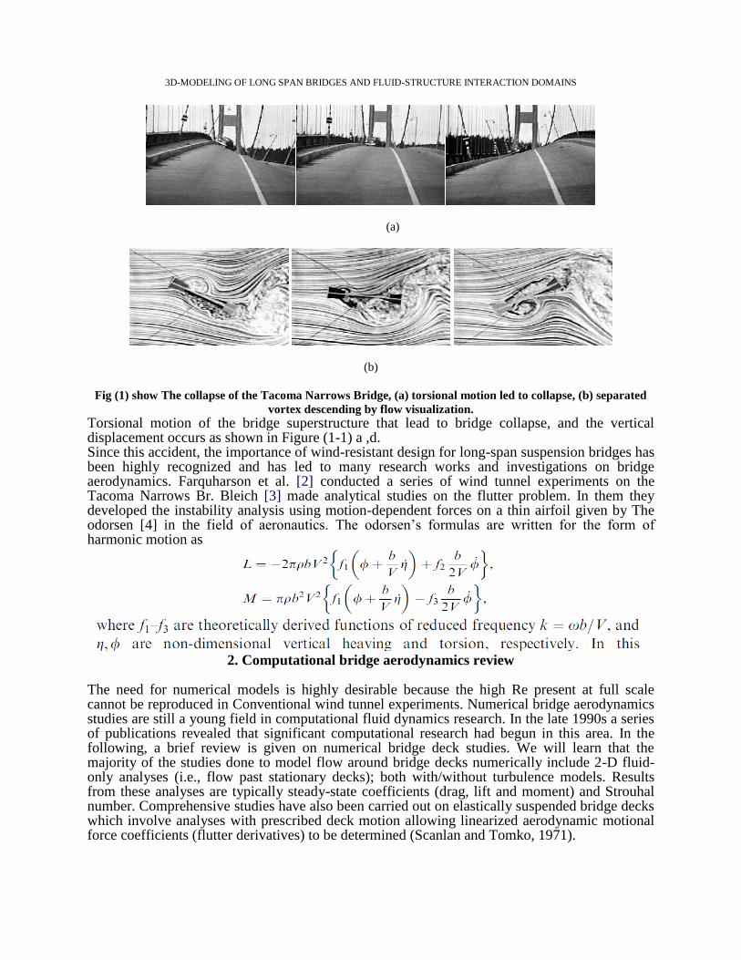
Figure (6 ) show the pressure distribution (a) in the 2D-Model and (b) in the 3D-Model. Dd222

In the case studies presented in the following section, prior to the full fluid–structure analyses of

moving bridge decks ,a series of simulations are undertaken to observe the unsteady flow

patterns around a stationary structure in an attempt to establish mesh-modeling criteria for the

flow phenomena of interest. The solution of the fluid equations results in computed pressures

and tractions which act on the bridge. The resulting forces on the bridge deck are then computed

by integrating the pressures and friction components along the boundary on the deck surfaces.

The net forces (per unit span) are usually expressed in a dimensionless form, and referred to as

the aerodynamic coefficients, the drag ; the lift and the moment

(a) (b)

Figure (7-a) show the momentum coefficients from 3D analysis, (7-b) A half 3D model with half Domain.

(a) (b)


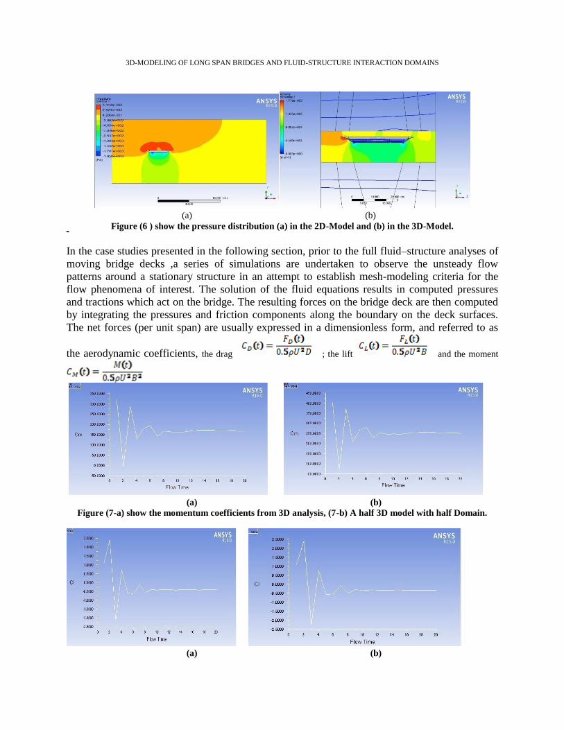
Figure (8-a) show the left coefficients from 3D analysis, (8-b) A half 3D model with half Domain.

(a) (b)

Figure (9-a) show the Drag coefficients from 3D analysis, (9-b) A half 3D model with half Domain.

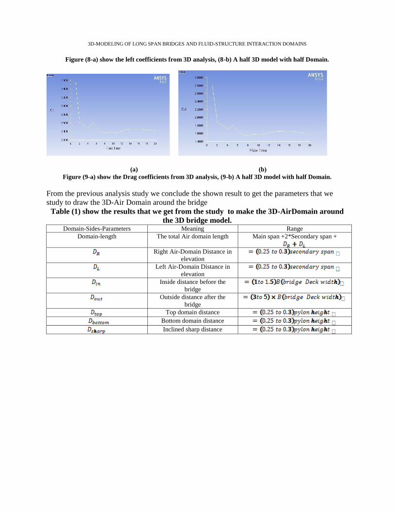
From the previous analysis study we conclude the shown result to get the parameters that we

study to draw the 3D-Air Domain around the bridge

Table (1) show the results that we get from the study to make the 3D-AirDomain around

the 3D bridge model. Domain-Sides-Parameters Meaning Range

Domain-length The total Air domain length Main span +2*Secondary span +

Right Air-Domain Distance in

elevation

Left Air-Domain Distance in

elevation

Inside distance before the

bridge

Outside distance after the

bridge

Top domain distance

Bottom domain distance

Inclined sharp distance



Structural Domain The structure considered is essentially 2-D, and is mounted on elastic springs with viscous dashpots appropriate to the structural mode of vibration under consideration.In effect, the structure is modelled as an elastic boundary condition embedded within the fluid domain.On this boundary, structural elements are attached to model a rigid bridge deck.The structural equations of motion for the dynamical behavior of a damped linear mechanical system with n degrees of freedom are

whereMs; Cs and Ks denote the mass, damping and stiffness matrices, and xsi and Fsi the displacements and fluid forces. The subscript i ¼ fx; y; yg denotes the horizontal, vertical and rotational directions.The right-hand side of Eq. (4) contains the resultants of the surface traction of fluid.Further we note that the fluid velocity is identical to the structural velocity ðusiÞ at the interface due to the specified no-slip condition.The matrix contents of Ms; Cs and Ks depend on whether the simulations are vortex-induced oscillations or flutter.In the flutter simulation, the vertical and rotational degrees of freedom couple and off-diagonal terms are included in the matrices.If large rotations occur during these simulations, extra stiffness terms are automatically generated through nonlinear specification in Spectrum.Using special lumped elements (in user-defined functions), stiffness and damping are specified through springs and dashpots and the mass is lumped.The Spectrum program was developed for 3-D models and therefore does not offer an interface between structural beam elements and fluid shell elements.Instead the structural elements are modelled using four-node quadrilateral elements, which are given an artificial high stiffness to simulate rigid bridge deck boundaries together with specified zero continuous mass.The fluid domain contains either eight-noded hexahedral or six-noded triangular prism elements.The major drawback of using Spectrum for 2-D modelling is a model which contains twice the numbers of nodes intended and therefore double the amount of equations to be solved.

The no-slip condition is prescribed along the fluid–structure interfaces.This means that the following velocity condition must be satisfied, Where: Usi and Ui represent the velocity fields of the structure and the fluid particles, respectively. In addition to the kinematic boundary conditions, it is also necessary to impose continuity of traction at the fluid–structure interfaces,

A plane-strain condition is used to simulate the structural domain in 2-D, i.e., the nodal boundary condition set for

all nodes of the deck is defined to consist of zero out-of-plane displacements and zero x- and y-rotations.

The fluid – structure interface Most fluid FE analyses are accomplished using the Eulerian description in which the mesh is fixed in space and the material particles flow through the mesh, as shown in Fig.3 (a).Each FE is crossed by the fluid flow. In an aero elastic analysis, the Eulerian description is inadequate as the domain surrounding the structure is itself in motion.The usual numerical representation for structural motion is the Lagrangian description in which the mesh motion coincides with the motion of the material particles, as illustrated in Fig.3 (b).The fluid domain is free to move, but the mesh movement and the velocity of the fluid particles are constrained to be the same. This may result in severe mesh distortions due to, for example, vortex-induced oscillations as each element always contain the same fluid particles. The ALE approach, supported by the general


kinematic theory in Hughes et al.(1981) , provides a method for the solution of the equations describing fluid flow through a moving mesh, as shown in Fig.3 (c). The nodes of the mesh are free to move independently of the fluid flow. The concept of the moving and deforming reference frame (ALE) has been introduced in finite differences by Noh (1964).Later, it was implemented in FEs by Donea et al.(1977) .Inthe ALE scheme, the convective term in the NSEs contains the relative velocity between particles and mesh.The specific application of the ALE scheme to a moving bridge deck is illustrated in Fig.4 .No deforming fluid domain boundaries are specified in the current FSI analyses, and the bridge deck is kept as a moving rigid body. In the present work flow simulation around a stationary bridge deck adopts adopts the Eulerian scheme in the entire fluid domain, whereas the simulations around a moving bridge deck adopt the ALE scheme in the whole fluid domain. Several investigators, among these Anju et al.(1997) , Mendes and Branco (1999) and Nomura and Hughes (1992), have described a way of reducing computations by having only a small part of the mesh around the structure as a moving ALE mesh, and the nonadjacent fluid mesh following the standard Eulerian scheme. The mesh motion is solved as a quasi-static problem from

Where: Km is the stiffness matrix which depends on the mesh movement xmi; if large deformations are encountered. The subscript i ¼ fx; y; yg denotes horizontal, vertical and rotation. We note the inertia and damping terms are not actually included in the solution process. It should be emphasized that the mesh formulation has no physical interpretation, i.e., terms such as Cauchy stresses and elastic moduli do not have the usual physical interpretation within this context. In effect, the mesh is modeled as an elastic solid, whose interior node positions are computed as if all nearest nodal neighbors were coupled by an elastic medium and which sets the positions and velocities of the boundary nodes to precisely match the boundary motions. In reality, it is a purely mathematical construct, i.e., a method for updating the mesh in such a way that it maintains integrity.

Note that the model does not absolutely guarantee mesh integrity, as it may be violated if very large deformations or twisting motions are simulated. In such cases, the problem must be remeshed. The boundary conditions for the FSI analyses are shown in Fig.2 .The domain Ds is the moving idealized rigid bridge deck supported on elastic springs, and Dx is the moving spatial domain of viscous incompressible fluid elements over which the fluid motion is described. For the FSI analyses, further boundary conditions are specified in the mesh equations to keep the fluid mesh in contact with the moving structure. It is through the specification of compatibility and equilibrium at the interfaces the fluid and the moving structure is achieved. Only a compatibility condition is imposed on the mesh equations, i.e., the mesh follows the structure and fluid interfaces.


Figure (11) F.E schemes : (a) Eulerian scheme, (b) Lagrangian scheme and (c) ALE scheme.


Figure (12) The ALE scheme applied to a wind moving bridge deck.

At the interfaces, continuity of displacement, velocity and traction fields must be satisfied for all times at all points on the boundary CI; where I denote the interface. CONCLUSION Long-span bridges require extensive wind tunnel testing. The objective of this research is to determine the 3D-Airodynamic model that make the computer model is very similar to the expensive physical model tests that are currently required to determine the aerodynamic cross-section of a single structure. This study describes the use of a coupled fluid–structure interaction (FSI) finite element (FE) solver. Aerodynamic effects of flutter-bridge motion are investigated using fluid and structural two-dimension FEs on moving non adaptive grids. The moving interface between fluid and structure is modelled through the arbitrary Lagrangian–Eulerian (ALE) formulation. First, simulation of fluid flow around a fixed bridge deck was simulated. The FE model was validated using different meshes for a range of high Reynolds numbers. Time-domain vortex-shedding analysis was presented. Some questions as to model accuracy were raised due to a discrepancy in Strouhal number compared to physical experiments. The reason being that the turbulent flow around the fixed deck problem was not captured reliably with the present viscous FE solver. However, it was shown, that the mechanisms of flutter are independent of the much higher-frequency bluff body shedding phenomenon and was therefore not explored any further in this study. Second, flutter simulations were presented showing the ability of the FE model to self-excite into flexural–torsional flutter. The FE simulations showed that, when the flutter limit is reached, the structure controls the fluid flow. The flutter limit of the long-span bridge deck was found to be in good agreement with the wind tunnel results and other numerical methods. Furthermore, it is also recognized that the flat-plate flutter theory of Theodore (1935) gives comparatively accurate solutions despite the assumption of in viscid flow, suggesting that accurate modeling of the boundary layer may not be so critical for this aero elastic phenomenon. The models used, despite the laminar flow assumption and the coarseness of the meshes compared to those of other investigators, may be close to what is required for this type of flow simulation, that is about 1900 nodes in an irregular unstructured grid. However, a higher CPU requirement, but not necessarily parallel processing, than those used here is desirable if the FE


ALE approach is to prove to be a viable supplementary tool to the wind tunnel. In conclusion, prediction of flutter instability for sharp edge bridge decks does not appear sensitive to turbulence and three-dimensional flow structure modeling. Acknowledgement I am very grateful to Prof.Dr.Walid Abd elateif, Department of structural engineering, Cairo University for the many help and advices that he give to me. REFERENCES 1. (1)-Anju, A., Maruoka, A., Kawahara, M., 1997. 2-D fluid–structure interaction problems

by an arbitrary Lagrangian )Eulerian finite element method.International Journal of Computational Fluid Dynamics 8, 1–9.

2. (2)Ansys Inc., 1999. Spectrum Solver (Version 2.0) Command Reference and Theory Manual. Ansys Inc., USA (Spectrum wascommercially available in 1993–1999 and is a registered trademark of Ansys Inc.).

3. (3)Brar, P.S., 1997. Numerical calculation of bluff body flutter derivatives via computational fluid dynamics. Ph.D. Thesis, The John Hopkins University, Baltimore, MD, USA.

4. (4)Bruno, L., Khris, S., Marcillat, J., 2001. Numerical simulation of the effect of section details and partial streamlining on the aerodynamics of bridge decks.Journal of Wind and Structures 4, 315–332.

5. (5)Chorin, A.J., 1989. Numerical study of slightly viscous flow. Journal of Fluid Mechanics 57(4), 785–796. 1973.

6. (6)Dahle, L.A., Reed, K., Aarsnes, J.V., 1990. Model tests with submerged floating tube bridges. In: Krokeborg, J. (Ed.), Proceedings of the Second Symposium on Strait Crossings.Balkema, Trondheim, Norway.

7. (7)De Foy, B., 1998. Unsteady incompressible flow solver with optimised operators. Ph.D. Thesis, Cambridge University, Department of Engineering, Cambridge, England.

8. (8)DMI and SINTEF, 1993a.Wind-tun nel tests. Storebælt East Bridge.Suspensio n bridge.Section model tests, II. Technical Report 92063.00.01, Danish Maritime Institute, Lyngby, Denmark (Used with permission from Storebælt A/S).

9. (9)DMI and SINTEF, 1993b.Wind-tunnel tests.Storebælt East Bridge.Tender evaluation, suspension bridge. Alternative sections.

10. (10)Section model tests, I. Technical Report 91023-10.00. Revision 0., Danish Maritime Institute, Lyngby, Denmark (Used with permission from Storebælt A/S). Donea, J., Fasoli-stella, P., Giuliani, S., 1977. Lagrangian and Eulerian finite element techniques for transient fluid–structure interaction problems. Transactio ns Fourth SMIRT Conference, San Fransisco, 15–19 August 1977, USA (Paper B1/2).

3D-Modeling of Long span Bridges and Fluid-Structure ...

Documents