C. R. Mecanique 335 (2007) 269–279 http://france.elsevier.com/direct/CRAS2B/ Melting and solidification: processes and models/Flows in solidification 3D macrosegregation simulation with anisotropic remeshing Sylvain Gouttebroze a , Michel Bellet a , Hervé Combeau b,∗ a CEMEF, École des mines de Paris, BP207, 06904 Sophia Antipolis cedex, France b LSG2M, Écoles des mines de Nancy, parc de Saurupt, 54000 Nancy, France Abstract The article presents a three-dimensional coupled numerical solution of momentum, mass, energy and solute conservation equations, for binary alloy solidification. The interdendritic flow in the mushy zone is assumed to obey the Darcy’s law. Mi- crosegregation is governed by the lever rule, assuming local equilibrium at phase interfaces. The resulting energy and solute advection–diffusion equations are solved using the Streamline-Upwind/Petrov–Galerkin (SUPG) finite element method. A SUPG- PSPG velocity-pressure formulation is applied for the momentum equation. The full algorithm was implemented in the 3D code THERCAST, together with an anisotropic remeshing method. Two applications have been considered: a small ingot of Pb-48wt%Sn alloy and a large steel ingot. The numerical results of these two cases are presented with the evolution of temperature, liquid veloc- ity, and solute concentration fields during solidification. To cite this article: S. Gouttebroze et al., C. R. Mecanique 335 (2007). © 2007 Académie des sciences. Published by Elsevier Masson SAS. All rights reserved. Résumé Simulation 3D de la macroségrégation avec remaillage anisotrope. Un modèle numérique de simulation des transferts couplés de chaleur, de masse et de quantité de mouvement pendant la solification d’un alliage binaire est présenté. Les équations du modèle sont classiques, l’écoulement du liquide interdendritrique est décrit par une loi de type Darcy. Le modèle des bras de levier (équilibre complet entre les phases liquide et solide) a été adopté pour la microsgégrégation. Le modèle numérique a été élaboré suivant la méthode des éléments finis pour des géométries tri-dimensionnelles dans le code THERCAST. Les équations de conservation de l’énergie et de la masse de soluté ont été discrétisées à l’aide d’un schéma SUPG et celles de la quantité de mouvement et de la masse totale par un schéma SUPG-PSPG. L’originalité de ce travail provient de la mise en oeuvre d’une méthode de maillage évolutif qui permet d’obtenir une bonne précision de calcul avec un nombre d’éléments de calcul raisonnable. Deux applications illustratives sont présentées, une première application concerne le cas d’un petit domaine pour un alliage Pb- 48wt%Sn et la deuxième, un lingot d’acier. Pour citer cet article : S. Gouttebroze et al., C. R. Mecanique 335 (2007). © 2007 Académie des sciences. Published by Elsevier Masson SAS. All rights reserved. Keywords: Computational fluid mechanics; Solidification; Macrosegregation; Finite element; Remeshing Mots-clés : Mécanique des fluides numérique ; Solidification ; Macroségrégation ; Eléments finis ; Remaillage * Corresponding author. E-mail addresses: [email protected] (S. Gouttebroze), [email protected] (H. Combeau). 1631-0721/$ – see front matter © 2007 Académie des sciences. Published by Elsevier Masson SAS. All rights reserved. doi:10.1016/j.crme.2007.05.005

Welcome message from author
This document is posted to help you gain knowledge. Please leave a comment to let me know what you think about it! Share it to your friends and learn new things together.
Transcript
C. R. Mecanique 335 (2007) 269–279
http://france.elsevier.com/direct/CRAS2B/
Melting and solidification: processes and models/Flows in solidification
3D macrosegregation simulation with anisotropic remeshing
Sylvain Gouttebroze a, Michel Bellet a, Hervé Combeau b,∗
a CEMEF, École des mines de Paris, BP207, 06904 Sophia Antipolis cedex, Franceb LSG2M, Écoles des mines de Nancy, parc de Saurupt, 54000 Nancy, France
Abstract
The article presents a three-dimensional coupled numerical solution of momentum, mass, energy and solute conservationequations, for binary alloy solidification. The interdendritic flow in the mushy zone is assumed to obey the Darcy’s law. Mi-crosegregation is governed by the lever rule, assuming local equilibrium at phase interfaces. The resulting energy and soluteadvection–diffusion equations are solved using the Streamline-Upwind/Petrov–Galerkin (SUPG) finite element method. A SUPG-PSPG velocity-pressure formulation is applied for the momentum equation. The full algorithm was implemented in the 3D codeTHERCAST, together with an anisotropic remeshing method. Two applications have been considered: a small ingot of Pb-48wt%Snalloy and a large steel ingot. The numerical results of these two cases are presented with the evolution of temperature, liquid veloc-ity, and solute concentration fields during solidification. To cite this article: S. Gouttebroze et al., C. R. Mecanique 335 (2007).© 2007 Académie des sciences. Published by Elsevier Masson SAS. All rights reserved.
Résumé
Simulation 3D de la macroségrégation avec remaillage anisotrope. Un modèle numérique de simulation des transferts couplésde chaleur, de masse et de quantité de mouvement pendant la solification d’un alliage binaire est présenté. Les équations dumodèle sont classiques, l’écoulement du liquide interdendritrique est décrit par une loi de type Darcy. Le modèle des bras delevier (équilibre complet entre les phases liquide et solide) a été adopté pour la microsgégrégation. Le modèle numérique a étéélaboré suivant la méthode des éléments finis pour des géométries tri-dimensionnelles dans le code THERCAST. Les équationsde conservation de l’énergie et de la masse de soluté ont été discrétisées à l’aide d’un schéma SUPG et celles de la quantité demouvement et de la masse totale par un schéma SUPG-PSPG. L’originalité de ce travail provient de la mise en oeuvre d’uneméthode de maillage évolutif qui permet d’obtenir une bonne précision de calcul avec un nombre d’éléments de calcul raisonnable.Deux applications illustratives sont présentées, une première application concerne le cas d’un petit domaine pour un alliage Pb-48wt%Sn et la deuxième, un lingot d’acier. Pour citer cet article : S. Gouttebroze et al., C. R. Mecanique 335 (2007).© 2007 Académie des sciences. Published by Elsevier Masson SAS. All rights reserved.
Keywords: Computational fluid mechanics; Solidification; Macrosegregation; Finite element; Remeshing
Mots-clés : Mécanique des fluides numérique ; Solidification ; Macroségrégation ; Eléments finis ; Remaillage
* Corresponding author.E-mail addresses: [email protected] (S. Gouttebroze), [email protected] (H. Combeau).
1631-0721/$ – see front matter © 2007 Académie des sciences. Published by Elsevier Masson SAS. All rights reserved.doi:10.1016/j.crme.2007.05.005
270 S. Gouttebroze et al. / C. R. Mecanique 335 (2007) 269–279
1. Introduction
Solidification of alloys generates the segregation of solutes (chemical species) at the scale of the microstructure,called microsegregation. This inhomogeneity can be redistributed by any driving force promoting a relative velocitybetween the solid and the liquid phases; this is called macrosegregation. Only the natural thermal and solutal convec-tion of the liquid phase has been considered in this work, the solid phase being considered as fixed. Macrosegregationcan affect mechanical and chemical properties and so its prediction is essential to optimize cast products. This phe-nomenon is particularly important in the solidification of large ingots. However, most three-dimensional simulationsare currently made on small ingots or pieces of about 10 centimeters high [1,2]. This is due to the fact that the flowfield is more complex and unstable in larger casting, and that a good accuracy in the prediction of macrosegregationrequires a fine mesh in the mushy zone. In order to overcome such difficulties, the main idea of the present contribu-tion relies on the implementation of an adaptive remeshing technique. This strategy allows a good accuracy combinedwith an optimal computational effort particularly for large ingot simulation.
The equations of the macrosegregation model and the strategy adopted in THERCAST, a three-dimensional finiteelement solidification code developed by CEMEF [3] are presented in the first part. Then, the remeshing method isdescribed. Finally, the capabilities of the method are illustrated on two cases: a small ingot reproducing the conditionsof the Hebditch–Hunt experiment for a Pb-48wt%Sn alloy and a large steel ingot of 2 m height with a pseudo-2Dapproach.
2. Conservation equations and discretization
The conservation equations for mass, momentum, solute and energy constitute the core of a macrosegregationmodel. These equations can be derived from three main approaches: volumetric averaging techniques [4], continuummodel of mixture theory [5], and stochastic averaging [6]. This last method has been used for this work. We referto [7] for a discussion on the range of validity of the different assumptions of the model. The conservation equationsare recalled and their finite element discretization is presented.
2.1. Conservation of mass and momentum
The main hypotheses of the mechanical model are the following:
– rigid and fixed solid phase;– the liquid is Newtonian, the viscosity constant and the flow laminar;– solid and liquid phase densities are equal (ρ = ρs = ρl) and constant (ρ = ρ0), except in the buoyancy term (ρ̃g)
according to the Boussinesq approximation. The density of the liquid phase depends on the temperature T andthe solute content in the liquid phase cl :
ρ̃ = ρ0[1 − βT (T − Tref) − βc(cl − cref
l )]
(1)
where βT and βc are the thermal and solutal expansion coefficients respectively, and ρ0 is the density in the liquidassumed constant. Tref is the reference temperature imposed equal to the liquidus temperature at the initial soluteconcentration in the liquid, cref
l ;– a saturated mixture, i.e.:
gs + gl = 1 (2)
where gs and gl are the solid and liquid volumetric fraction respectively;– the mushy region is modelled as an isotropic porous medium whose permeability, K , is defined by the Carman–
Kozeny formula:
K = λ22g
3l
180(1 − gl)2(3)
One can notice that λ2 in Eq. (3) corresponds to a characteristic size of the microstructure in the mushy zone, whichis generally estimated as an average secondary dendrite arm spacing. More complex models of permeability [8] are
S. Gouttebroze et al. / C. R. Mecanique 335 (2007) 269–279 271
available in the literature and could be easily implemented in the model. The choice of this permeability law has beendone mainly for comparison reasons with previous results (from Refs. [1] and [14]).
Due to the fact that the densities of the solid and liquid phases are equal and constant, notably shrinkage is ne-glected, the mass conservation equation is reduced to:
∇ · V = 0 (4)
where V is the so-called mixture velocity. According to Eq. (2) we have: V = glVl + gsVs = glVl.As presented in a previous paper [9], the classical mixture theory [5] yields to the following momentum conserva-
tion equation:
ρ0dVdt
= ∇ · (μ∇V) − ∇P + ρ̃g − μ
KV (5)
where V and P are the unknown velocity and pressure fields, and μ is the dynamic viscosity of the liquid.A SUPG-PSPG formulation has been used to discretise the momentum equation together with the mass conserva-
tion equation. The SUPG-PSPG formulation, presented for CFD finite element calculations by Tezduyar et al. [10],is based on three stabilization coefficients: a τSUPG coefficient (Streamline-Upwind/Petrov–Galerkin), a τPSPG coeffi-cient (Pressure-Stabilizing/Petrov–Galerkin) and a τLSIC coefficient (least-squares on incompressibility constraint) aspresented in Eq. (6).∫
Ω
(ρ0
∂V∂t
+ ρ0∇ · (V × V) − ∇ · (μ∇V) + μ
KV − ρ̃g
)· V∗ dΩ +
∫Ω
P ∗∇ · V dΩ
+nelt∑e=1
∫Ωe
(ρ0
∂V∂t
+ ρ0∇ · (V × V) − ∇ · (μ∇V) + μ
KV − ρ̃g
)· 1
ρ0(τSUPGρ0V · ∇V∗ + τPSPG∇P ∗)dΩ
+nelt∑e=1
∫Ωe
τLSIC∇ · V∗ρ0∇ · V dΩ = 0 (6)
where V∗ and P ∗ are the test functions of the finite elements for the velocity and pressure fields respectively. Thestabilisation coefficients (τSUPG, τPSPG and τLSIC) depend on the local mesh size, which is calculated in the flowdirection. As this isotropic stabilisation is applied on anisotropic mesh, the accuracy of the solution might be affected.However, in the remeshing strategy, presented in the next section, the stretching of the elements is limited and so isthe possible inaccuracy.
2.2. Energy conservation equation
Using the above hypotheses, the energy balance can be written in the form:
∂H
∂t+ V · ∇(ρcpT ) − ∇ · (k∇T ) = 0 (7)
Assuming that the specific heat cp is constant and equal for the liquid and solid phases, T is related to the averagevolumic enthalpy H by the following equation:
H = cp(T − T0) + gl�Hls (8)
where �Hls is the latent heat of fusion. Eq. (7) is a non-linear equation in enthalpy. Thus this equation is solved usinga Newton–Raphson scheme with a Euler-backward time discretization.
2.3. Solute mass conservation equation
The present model of binary alloy solidification assumes that the phase diagram is linearized (constant liquidusslope and constant partition coefficient). At the scale of the microstructure, the solid and liquid phases are assumed tobe at thermodynamic equilibrium (lever rule), which yields the equilibrium relations:
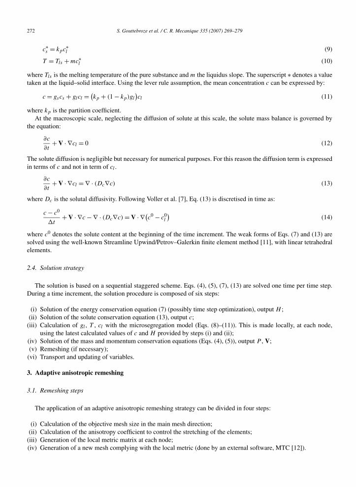
272 S. Gouttebroze et al. / C. R. Mecanique 335 (2007) 269–279
c∗s = kpc∗
l (9)
T = Tls + mc∗l (10)
where Tls is the melting temperature of the pure substance and m the liquidus slope. The superscript ∗ denotes a valuetaken at the liquid–solid interface. Using the lever rule assumption, the mean concentration c can be expressed by:
c = gscs + glcl = (kp + (1 − kp)gl
)cl (11)
where kp is the partition coefficient.At the macroscopic scale, neglecting the diffusion of solute at this scale, the solute mass balance is governed by
the equation:
∂c
∂t+ V · ∇cl = 0 (12)
The solute diffusion is negligible but necessary for numerical purposes. For this reason the diffusion term is expressedin terms of c and not in term of cl .
∂c
∂t+ V · ∇cl = ∇ · (Dc∇c) (13)
where Dc is the solutal diffusivity. Following Voller et al. [7], Eq. (13) is discretised in time as:
c − c0
�t+ V · ∇c − ∇ · (Dc∇c) = V · ∇(
c0 − c0l
)(14)
where c0 denotes the solute content at the beginning of the time increment. The weak forms of Eqs. (7) and (13) aresolved using the well-known Streamline Upwind/Petrov–Galerkin finite element method [11], with linear tetrahedralelements.
2.4. Solution strategy
The solution is based on a sequential staggered scheme. Eqs. (4), (5), (7), (13) are solved one time per time step.During a time increment, the solution procedure is composed of six steps:
(i) Solution of the energy conservation equation (7) (possibly time step optimization), output H ;(ii) Solution of the solute conservation equation (13), output c;
(iii) Calculation of gl , T , cl with the microsegregation model (Eqs. (8)–(11)). This is made locally, at each node,using the latest calculated values of c and H provided by steps (i) and (ii);
(iv) Solution of the mass and momentum conservation equations (Eqs. (4), (5)), output P , V;(v) Remeshing (if necessary);
(vi) Transport and updating of variables.
3. Adaptive anisotropic remeshing
3.1. Remeshing steps
The application of an adaptive anisotropic remeshing strategy can be divided in four steps:
(i) Calculation of the objective mesh size in the main mesh direction;(ii) Calculation of the anisotropy coefficient to control the stretching of the elements;
(iii) Generation of the local metric matrix at each node;(iv) Generation of a new mesh complying with the local metric (done by an external software, MTC [12]).
S. Gouttebroze et al. / C. R. Mecanique 335 (2007) 269–279 273
3.2. Metric definition
A metric M is represented by a symmetric, definite positive (3, 3) matrix (for a 3D case), which is used to calculatescalar products and hence distances. Given a vector u, the norm of u according to the metric M is defined by:
‖u‖M =√
uT · M · u (15)
So when using a locally defined metric M (varying with spatial coordinates), the distance between two points isdependent on their position. This allows a control of the mesh size in the different spatial directions because themesher tries to obtain a uniform mesh (using the metric to calculate the size of the elements). The generation of thelocal metric at each node is performed in two steps: first an objective mesh size h is computed and then the orientationand the elongation of the new mesh are calculated. Then the metric matrix is build:
M = RT ·⎛⎜⎝
1h2 0 0
0 1(coef·h)2 0
0 0 1(coef·h)2
⎞⎟⎠ · R (16)
where R is the rotation matrix defined by the main direction vector and two perpendicular vectors, coef is the valueof the elongation ratio.
3.3. Objective mesh size
A main direction is defined locally. The direction of a gradient or of the velocity of the liquid is used to determine it.The procedure is described in the next section. The objective mesh size is the size of the element in the main directionprescribed by the adaptation procedure. The local mesh size is determined by three criteria for mushy and liquid areas:
– gradient of liquid fraction, ‖∇gl‖;– gradient of mean concentration, ‖∇c‖;– gradient of the velocity norm, ‖∇‖V‖‖.
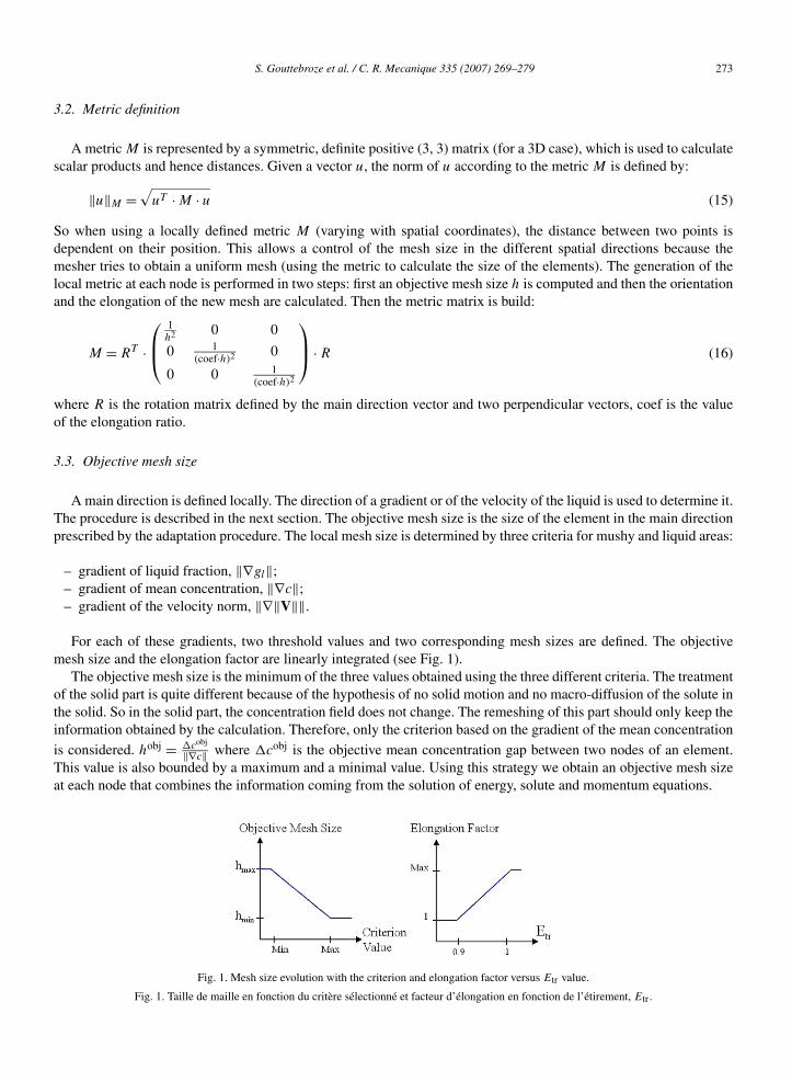
For each of these gradients, two threshold values and two corresponding mesh sizes are defined. The objectivemesh size and the elongation factor are linearly integrated (see Fig. 1).
The objective mesh size is the minimum of the three values obtained using the three different criteria. The treatmentof the solid part is quite different because of the hypothesis of no solid motion and no macro-diffusion of the solute inthe solid. So in the solid part, the concentration field does not change. The remeshing of this part should only keep theinformation obtained by the calculation. Therefore, only the criterion based on the gradient of the mean concentration
is considered. hobj = �cobj
‖∇c‖ where �cobj is the objective mean concentration gap between two nodes of an element.This value is also bounded by a maximum and a minimal value. Using this strategy we obtain an objective mesh sizeat each node that combines the information coming from the solution of energy, solute and momentum equations.
Fig. 1. Mesh size evolution with the criterion and elongation factor versus Etr value.
Fig. 1. Taille de maille en fonction du critère sélectionné et facteur d’élongation en fonction de l’étirement, Etr.
274 S. Gouttebroze et al. / C. R. Mecanique 335 (2007) 269–279
3.4. Anisotropy factors
The local anisotropy factors are the orientation of the mesh and the elongation factor. The first controls the directionin which the objective mesh size is applied and the second determines the objective mesh size in the two otherdirections. The calculation of the anisotropy is independent of the mesh size calculation, so different criteria areapplied. The domain is divided in three different areas:
– the solid zone, controlled by the mean concentration gradient;– the mushy zone, controlled by the liquid fraction gradient;– the liquid zone, controlled by the velocity.
In each zone the main mesh direction is given by the unitary vector collinear to the relevant vector (e.g. the velocityvector in liquid zone). Then, the elongation factor is calculated using the change in direction of these vectors in anelement following this formula:
Etr = maxk=1,4
(Vk · Vcenter
‖Vk‖‖Vcenter‖)
(17)
where k denotes the local node numbering and Vcenter denotes the velocity at the center of the element. After calcu-lating the elongation factor, according to Fig. 1, the objective mesh size is multiplied by the elongation factor in thedirections perpendicular to the mesh direction. On the other hand, in the liquid zone, the elongation factor is appliedin the direction of the velocity. The metric is built using all these elements and sent to the remesher MTC, which willoptimize the mesh topology using the local metric matrix.
3.5. Automatic control of the number of elements
Currently the remeshing is applied periodically; this period is fixed by the user. However, to avoid a huge increaseof the number of elements, a control function has been added. After each remeshing we estimate the new correctionfactor and the corrected mesh size as followed:
f newcorr =
(nelt
nobjelt
)1/3
· f oldcorr and hcorr
obj = f newcorr · hobj (18)
where nelt is the current number of elements and nobjelt the objective number of elements prescribed by the user. So the
minimum mesh size evolves during the calculation as illustrated in the second application case, resulting in a numberof elements maintained approximately constant. The minimum mesh size is reduced because the refined areas aregrowing due to the increasing complexity of the flow and the enlargement of the mushy zone and the correspondingboundary layer.
4. Applications
Two cases are presented in this section. For these two cases, a pseudo-2D approach has been used to shorten thecalculation time. In this approach we consider that this is a plane case, and we impose two symmetry planes and useonly one element in the thickness direction. Moreover, for the first case a full 3D computation has been performed.
4.1. Pb-48wt%Sn ingot
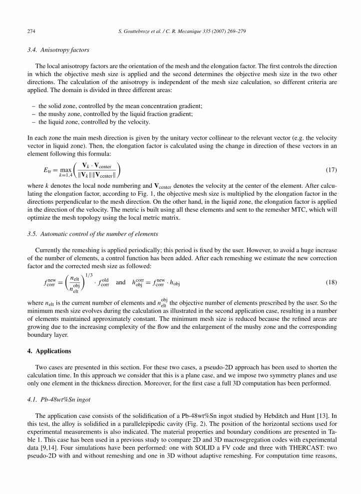
The application case consists of the solidification of a Pb-48wt%Sn ingot studied by Hebditch and Hunt [13]. Inthis test, the alloy is solidified in a parallelepipedic cavity (Fig. 2). The position of the horizontal sections used forexperimental measurements is also indicated. The material properties and boundary conditions are presented in Ta-ble 1. This case has been used in a previous study to compare 2D and 3D macrosegregation codes with experimentaldata [9,14]. Four simulations have been performed: one with SOLID a FV code and three with THERCAST: twopseudo-2D with and without remeshing and one in 3D without adaptive remeshing. For computation time reasons,
S. Gouttebroze et al. / C. R. Mecanique 335 (2007) 269–279 275
Fig. 2. Hebditch–Hunt case geometry.
Fig. 2. Géométrie du cas test Hebditch–Hunt.
Table 1Material properties and physical parameters for the Pb-48wt%Sn ingot
Tableau 1Propriétés du matériau et paramètres physiques pour le lingot utilisant l’alliage Pb-48wt%Sn
Thermal conductivity k 50 W m−1 K−1 Initial temperature Tinit 216 ◦CSpecific heat cp 200 J kg−1 K−1 Initial concentration c0 48 wt%Latent heat of fusion �Hls 53.5 kJ kg−1 Reference density ρ0 9000 kg m−3
Melting temperature Tls 327.5 ◦C Dynamic viscosity μ 10−3 Pa sLiquidus line slope m −2.3 K (wt%)−1 Dendrite arm spacing λ2 40 µmPartition coefficient kp 0.307 Heat convection coefficient h 400 W m−2 K−1
Eutectic temperature Teut 183 ◦C Thermal expansion coefficient βT 10−4 K−1
External temperature Text 25 ◦C Solutal expansion coefficient βT 4.5 × 10⁻³ (wt%)−1
Solutal diffusivity Dc 10−9 m2 s−1
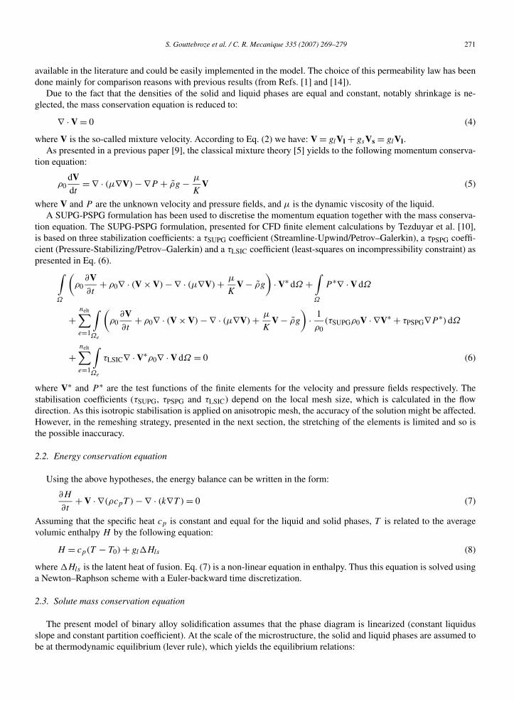
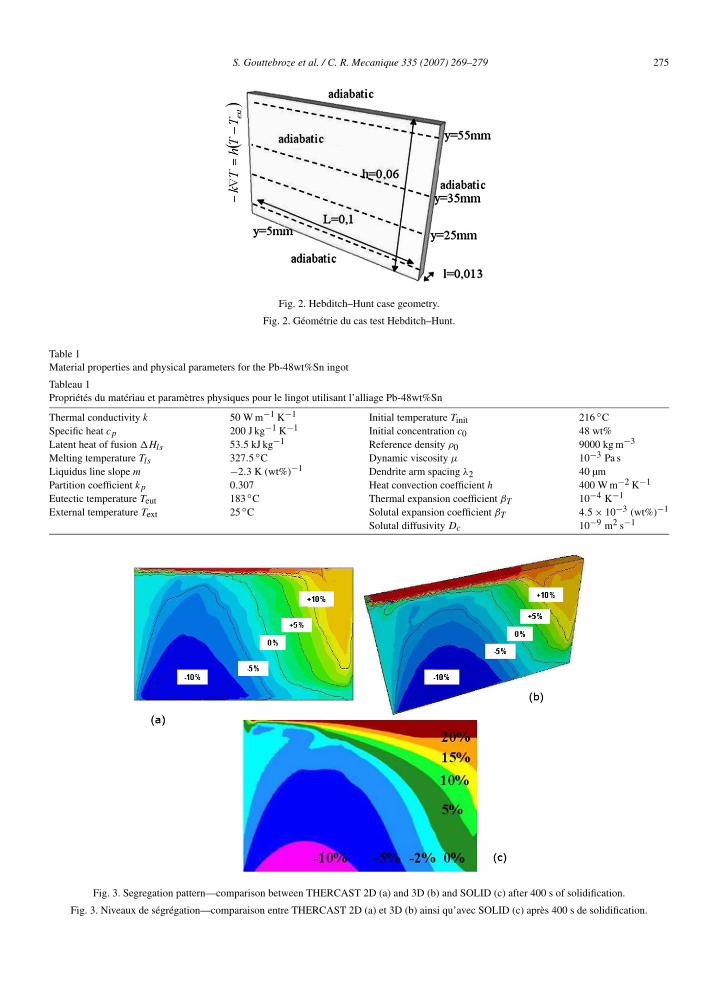
Fig. 3. Segregation pattern—comparison between THERCAST 2D (a) and 3D (b) and SOLID (c) after 400 s of solidification.
Fig. 3. Niveaux de ségrégation—comparaison entre THERCAST 2D (a) et 3D (b) ainsi qu’avec SOLID (c) après 400 s de solidification.
276 S. Gouttebroze et al. / C. R. Mecanique 335 (2007) 269–279
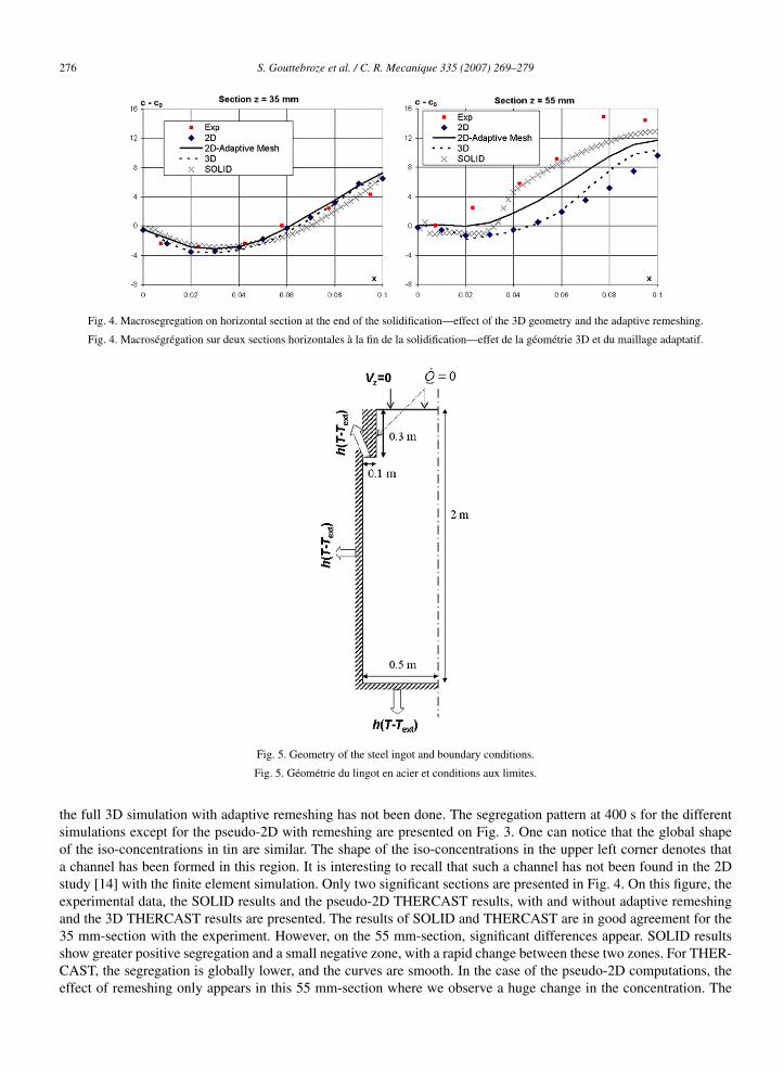
Fig. 4. Macrosegregation on horizontal section at the end of the solidification—effect of the 3D geometry and the adaptive remeshing.
Fig. 4. Macroségrégation sur deux sections horizontales à la fin de la solidification—effet de la géométrie 3D et du maillage adaptatif.
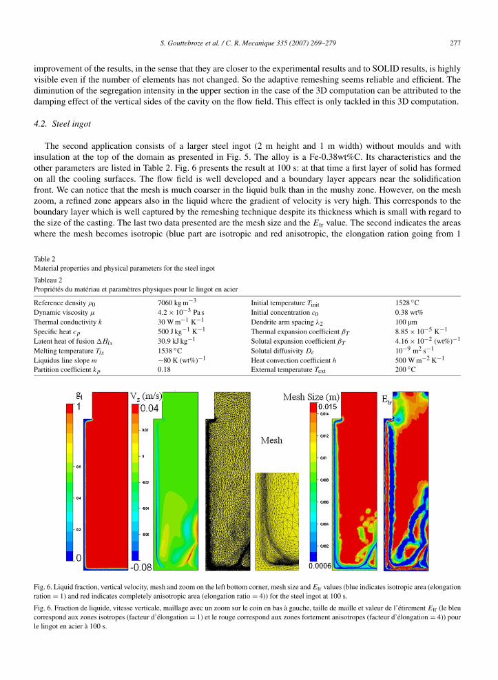
Fig. 5. Geometry of the steel ingot and boundary conditions.
Fig. 5. Géométrie du lingot en acier et conditions aux limites.
the full 3D simulation with adaptive remeshing has not been done. The segregation pattern at 400 s for the differentsimulations except for the pseudo-2D with remeshing are presented on Fig. 3. One can notice that the global shapeof the iso-concentrations in tin are similar. The shape of the iso-concentrations in the upper left corner denotes thata channel has been formed in this region. It is interesting to recall that such a channel has not been found in the 2Dstudy [14] with the finite element simulation. Only two significant sections are presented in Fig. 4. On this figure, theexperimental data, the SOLID results and the pseudo-2D THERCAST results, with and without adaptive remeshingand the 3D THERCAST results are presented. The results of SOLID and THERCAST are in good agreement for the35 mm-section with the experiment. However, on the 55 mm-section, significant differences appear. SOLID resultsshow greater positive segregation and a small negative zone, with a rapid change between these two zones. For THER-CAST, the segregation is globally lower, and the curves are smooth. In the case of the pseudo-2D computations, theeffect of remeshing only appears in this 55 mm-section where we observe a huge change in the concentration. The
S. Gouttebroze et al. / C. R. Mecanique 335 (2007) 269–279 277
improvement of the results, in the sense that they are closer to the experimental results and to SOLID results, is highlyvisible even if the number of elements has not changed. So the adaptive remeshing seems reliable and efficient. Thediminution of the segregation intensity in the upper section in the case of the 3D computation can be attributed to thedamping effect of the vertical sides of the cavity on the flow field. This effect is only tackled in this 3D computation.
4.2. Steel ingot
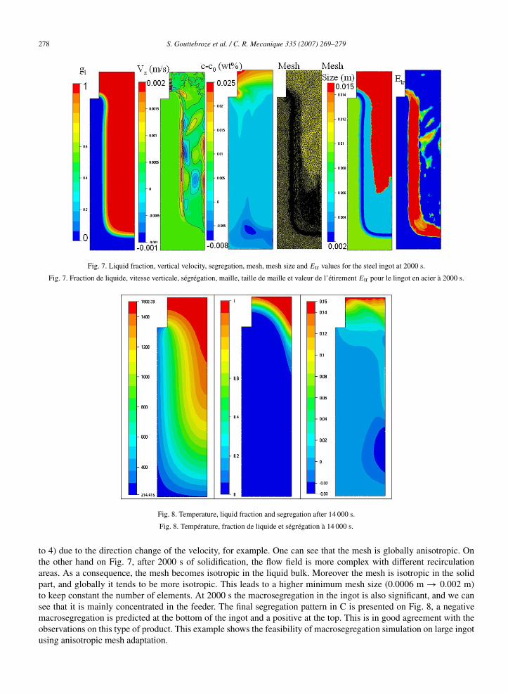
The second application consists of a larger steel ingot (2 m height and 1 m width) without moulds and withinsulation at the top of the domain as presented in Fig. 5. The alloy is a Fe-0.38wt%C. Its characteristics and theother parameters are listed in Table 2. Fig. 6 presents the result at 100 s: at that time a first layer of solid has formedon all the cooling surfaces. The flow field is well developed and a boundary layer appears near the solidificationfront. We can notice that the mesh is much coarser in the liquid bulk than in the mushy zone. However, on the meshzoom, a refined zone appears also in the liquid where the gradient of velocity is very high. This corresponds to theboundary layer which is well captured by the remeshing technique despite its thickness which is small with regard tothe size of the casting. The last two data presented are the mesh size and the Etr value. The second indicates the areaswhere the mesh becomes isotropic (blue part are isotropic and red anisotropic, the elongation ration going from 1
Table 2Material properties and physical parameters for the steel ingot
Tableau 2Propriétés du matériau et paramètres physiques pour le lingot en acier
Reference density ρ0 7060 kg m−3 Initial temperature Tinit 1528 ◦CDynamic viscosity μ 4.2 × 10⁻³ Pa s Initial concentration c0 0.38 wt%Thermal conductivity k 30 W m−1 K−1 Dendrite arm spacing λ2 100 µmSpecific heat cp 500 J kg−1 K−1 Thermal expansion coefficient βT 8.85 × 10⁻⁵ K−1
Latent heat of fusion �Hls 30.9 kJ kg−1 Solutal expansion coefficient βT 4.16 × 10⁻² (wt%)−1
Melting temperature Tls 1538 ◦C Solutal diffusivity Dc 10−9 m2 s−1
Liquidus line slope m −80 K (wt%)−1 Heat convection coefficient h 500 W m−2 K−1
Partition coefficient kp 0.18 External temperature Text 200 ◦C
Fig. 6. Liquid fraction, vertical velocity, mesh and zoom on the left bottom corner, mesh size and Etr values (blue indicates isotropic area (elongationration = 1) and red indicates completely anisotropic area (elongation ratio = 4)) for the steel ingot at 100 s.
Fig. 6. Fraction de liquide, vitesse verticale, maillage avec un zoom sur le coin en bas à gauche, taille de maille et valeur de l’étirement Etr (le bleucorrespond aux zones isotropes (facteur d’élongation = 1) et le rouge correspond aux zones fortement anisotropes (facteur d’élongation = 4)) pourle lingot en acier à 100 s.
278 S. Gouttebroze et al. / C. R. Mecanique 335 (2007) 269–279
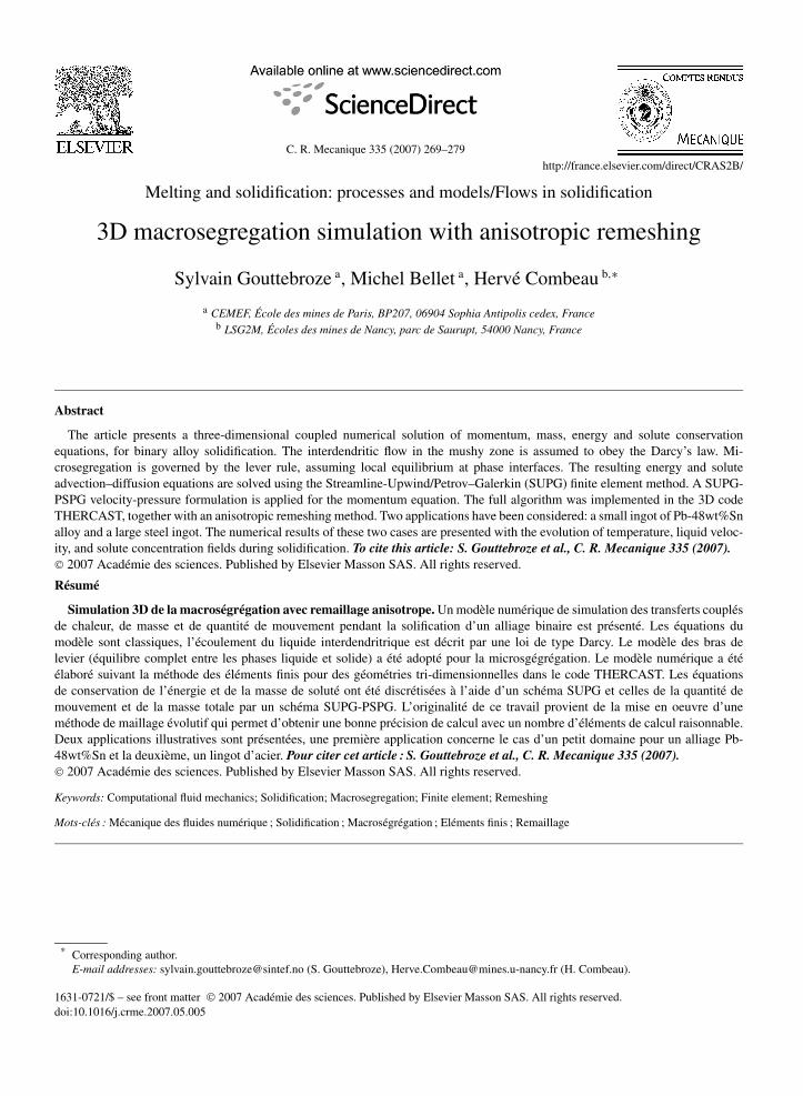
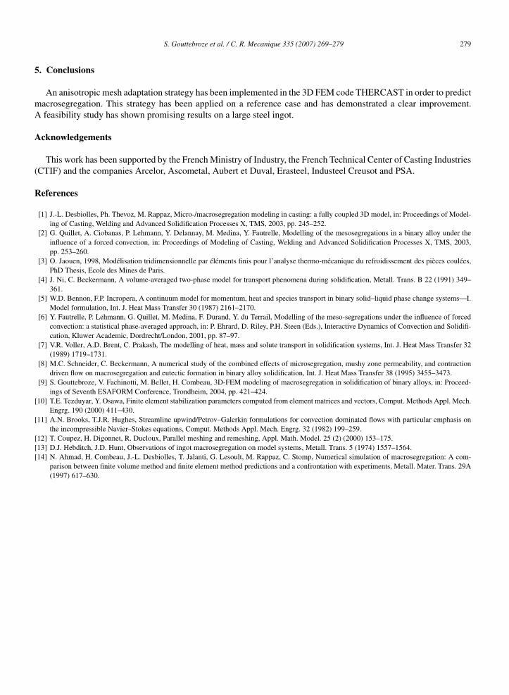
Fig. 7. Liquid fraction, vertical velocity, segregation, mesh, mesh size and Etr values for the steel ingot at 2000 s.
Fig. 7. Fraction de liquide, vitesse verticale, ségrégation, maille, taille de maille et valeur de l’étirement Etr pour le lingot en acier à 2000 s.
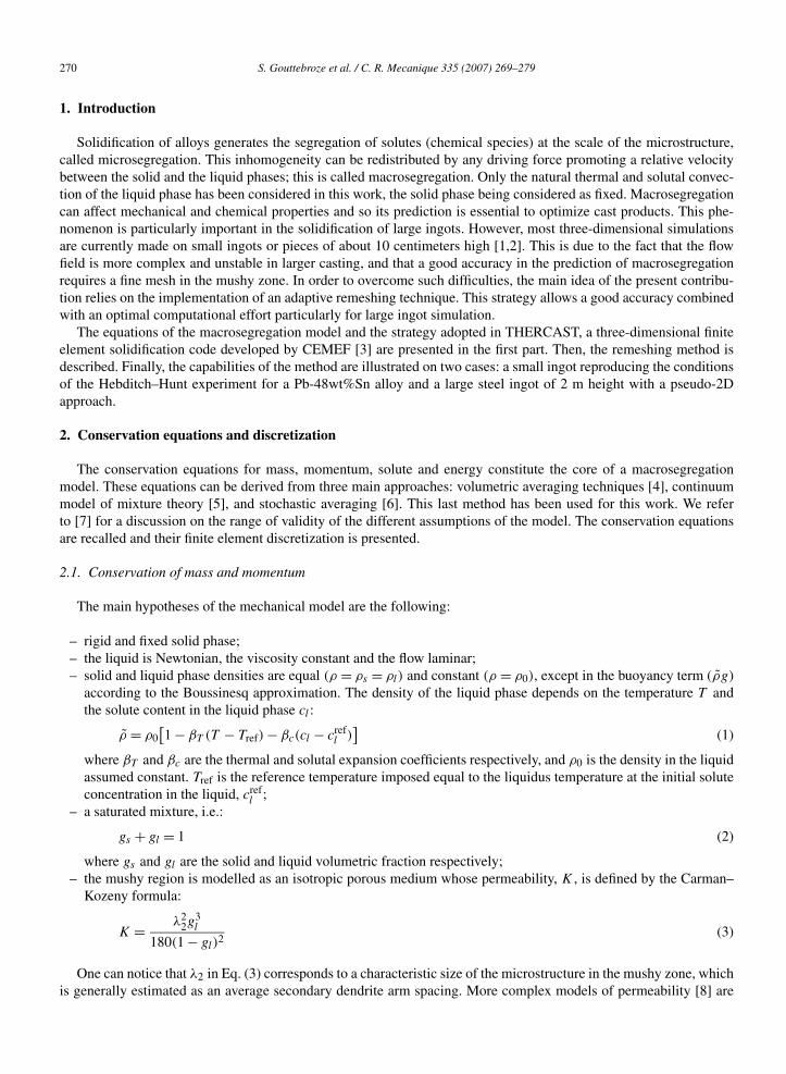
Fig. 8. Temperature, liquid fraction and segregation after 14 000 s.
Fig. 8. Température, fraction de liquide et ségrégation à 14 000 s.
to 4) due to the direction change of the velocity, for example. One can see that the mesh is globally anisotropic. Onthe other hand on Fig. 7, after 2000 s of solidification, the flow field is more complex with different recirculationareas. As a consequence, the mesh becomes isotropic in the liquid bulk. Moreover the mesh is isotropic in the solidpart, and globally it tends to be more isotropic. This leads to a higher minimum mesh size (0.0006 m → 0.002 m)to keep constant the number of elements. At 2000 s the macrosegregation in the ingot is also significant, and we cansee that it is mainly concentrated in the feeder. The final segregation pattern in C is presented on Fig. 8, a negativemacrosegregation is predicted at the bottom of the ingot and a positive at the top. This is in good agreement with theobservations on this type of product. This example shows the feasibility of macrosegregation simulation on large ingotusing anisotropic mesh adaptation.
S. Gouttebroze et al. / C. R. Mecanique 335 (2007) 269–279 279
5. Conclusions
An anisotropic mesh adaptation strategy has been implemented in the 3D FEM code THERCAST in order to predictmacrosegregation. This strategy has been applied on a reference case and has demonstrated a clear improvement.A feasibility study has shown promising results on a large steel ingot.
Acknowledgements
This work has been supported by the French Ministry of Industry, the French Technical Center of Casting Industries(CTIF) and the companies Arcelor, Ascometal, Aubert et Duval, Erasteel, Industeel Creusot and PSA.
References
[1] J.-L. Desbiolles, Ph. Thevoz, M. Rappaz, Micro-/macrosegregation modeling in casting: a fully coupled 3D model, in: Proceedings of Model-ing of Casting, Welding and Advanced Solidification Processes X, TMS, 2003, pp. 245–252.
[2] G. Quillet, A. Ciobanas, P. Lehmann, Y. Delannay, M. Medina, Y. Fautrelle, Modelling of the mesosegregations in a binary alloy under theinfluence of a forced convection, in: Proceedings of Modeling of Casting, Welding and Advanced Solidification Processes X, TMS, 2003,pp. 253–260.
[3] O. Jaouen, 1998, Modélisation tridimensionnelle par éléments finis pour l’analyse thermo-mécanique du refroidissement des pièces coulées,PhD Thesis, Ecole des Mines de Paris.
[4] J. Ni, C. Beckermann, A volume-averaged two-phase model for transport phenomena during solidification, Metall. Trans. B 22 (1991) 349–361.
[5] W.D. Bennon, F.P. Incropera, A continuum model for momentum, heat and species transport in binary solid–liquid phase change systems—I.Model formulation, Int. J. Heat Mass Transfer 30 (1987) 2161–2170.
[6] Y. Fautrelle, P. Lehmann, G. Quillet, M. Medina, F. Durand, Y. du Terrail, Modelling of the meso-segregations under the influence of forcedconvection: a statistical phase-averaged approach, in: P. Ehrard, D. Riley, P.H. Steen (Eds.), Interactive Dynamics of Convection and Solidifi-cation, Kluwer Academic, Dordrecht/London, 2001, pp. 87–97.
[7] V.R. Voller, A.D. Brent, C. Prakash, The modelling of heat, mass and solute transport in solidification systems, Int. J. Heat Mass Transfer 32(1989) 1719–1731.
[8] M.C. Schneider, C. Beckermann, A numerical study of the combined effects of microsegregation, mushy zone permeability, and contractiondriven flow on macrosegregation and eutectic formation in binary alloy solidification, Int. J. Heat Mass Transfer 38 (1995) 3455–3473.
[9] S. Gouttebroze, V. Fachinotti, M. Bellet, H. Combeau, 3D-FEM modeling of macrosegregation in solidification of binary alloys, in: Proceed-ings of Seventh ESAFORM Conference, Trondheim, 2004, pp. 421–424.
[10] T.E. Tezduyar, Y. Osawa, Finite element stabilization parameters computed from element matrices and vectors, Comput. Methods Appl. Mech.Engrg. 190 (2000) 411–430.
[11] A.N. Brooks, T.J.R. Hughes, Streamline upwind/Petrov–Galerkin formulations for convection dominated flows with particular emphasis onthe incompressible Navier–Stokes equations, Comput. Methods Appl. Mech. Engrg. 32 (1982) 199–259.
[12] T. Coupez, H. Digonnet, R. Ducloux, Parallel meshing and remeshing, Appl. Math. Model. 25 (2) (2000) 153–175.[13] D.J. Hebditch, J.D. Hunt, Observations of ingot macrosegregation on model systems, Metall. Trans. 5 (1974) 1557–1564.[14] N. Ahmad, H. Combeau, J.-L. Desbiolles, T. Jalanti, G. Lesoult, M. Rappaz, C. Stomp, Numerical simulation of macrosegregation: A com-
parison between finite volume method and finite element method predictions and a confrontation with experiments, Metall. Mater. Trans. 29A(1997) 617–630.
Related Documents