388023.pdf - University of Bristol Research Portal

This electronic thesis or dissertation has beendownloaded from Explore Bristol Research,http://research-information.bristol.ac.uk

Author:Wee, Victor Eng Lye

Title:An analysis of tax reform in Malaysia.

General rightsAccess to the thesis is subject to the Creative Commons Attribution - NonCommercial-No Derivatives 4.0 International Public License. Acopy of this may be found at https://creativecommons.org/licenses/by-nc-nd/4.0/legalcode This license sets out your rights and therestrictions that apply to your access to the thesis so it is important you read this before proceeding.

Take down policySome pages of this thesis may have been removed for copyright restrictions prior to having it been deposited in Explore Bristol Research.However, if you have discovered material within the thesis that you consider to be unlawful e.g. breaches of copyright (either yours or that ofa third party) or any other law, including but not limited to those relating to patent, trademark, confidentiality, data protection, obscenity,defamation, libel, then please contact [email protected] and include the following information in your message:

•Your contact details•Bibliographic details for the item, including a URL•An outline nature of the complaint

Your claim will be investigated and, where appropriate, the item in question will be removed from public view as soon as possible.

AN ANALYSIS OF TAX REFORM IN MALAYSIA

Victor Eng Lye WEE Department of Economics

University of Bristol

A thesis submitted to the University of Bristol in accordance with the requirements for the degree of

Doctor of Philosophy, in the Faculty of Social Sciences, May 1997

Resubmit June 1997

ABSTRACT

This thesis considers the implications of reforming the tax system of a developing

country, using Malaysia as the case study. It examines two main issues. First is to

analyse the macroeconomic effects of reforming the tax system, and second is to estimate the l. abour supply functions with taxation at the microeconomic level.

The thesis reviews the literature on the experiences of other countries in tax

reform. It examines in detail the Malaysian macroeconomy and tax system to gain an insight into the processes and interactions between economic performance, fiscal policy,

and tax structure for the last twenty five years.

In examining the first main issue, the computable general equilibrium (CGE)

model is used to perform counterfactual analysis of tax reforms on the Malaysian

economy. From the simulations on revenue-enhancing tax reform, we found that

corporate tax would be the best instrument to raise revenue without hurting households

or negatively affecting GDP aggregates. The simulations on revenue-neutral tax reform

showed that the current tax system could be made more efficient by changing the

structure of direct taxes and adopting VAT.

On the second issue, we adopt the instrumental variable approach with selectivity

adjustment to estimate the parameters of labour supply with taxation for Malaysia. The

modelling procedure estimates the equations for participation, wage, and hours of work.

The results show that the effect of taxes on the Malaysian labour supply response is

weak. In addition, the labour supply curve is backward bending starting from the lowest

wage level. Without the welfare and benefit system found in Western societies, workers

with low wages increase their hours of work in order to reach an income level that could

meet their household consumption needs.

ii

ACKNOWLEDGEMENTS

I am very pleased to acknowledge the guidance and help of my supervisors, David

Demery and Professor Andrew Chesher, in the preparation of this thesis as well as

throughout my study at Bristol. I am deeply indebted to them for their continual support

and encouragement, programming assistance, as well as invaluable comments. I am

grateful for the help given by Dr. Frank Harrigan at the Asian Development Bank on the

CGE model. I benefited from the input of members of the Economics Department who

had made helpful contributions.

I thank the Malaysian Federal Government for the financial support. I

acknowledge with gratitude the permission granted by the Economic Planning Unit of

the Prime Minister's Department, Malaysia, for allowing me access to the national

survey data. I would particularly like to thank Tan Sri Ali Abul Hassan bin Sulaiman and

Dato Annuar Ma'aruf at EPU, as well as Encik Zainol Abidin Abdul Rashid for

encouraging me to pursue Ph. D. I am grateful to Dr. Wan Abdul Aziz bin Wan Abdullah,

K. Govindan, Lynn Gosewell, Katherine Davis, Teo Thiam Teng (Chang Qing Shih), Ma

Bee Bian, Regina Lee, Loh Thiam Huat, and Royce Yee, the residents at Richmond

Terrace (where I served as a Senior Resident for three years), and the research students at

the Economics Department for their support, concern and good spirit. I am also grateful

to Fun Swee Pin for his weekly e-mail correspondence, which provided me a good

diversion from economics, and Tony Au who brought the Pentium computer into my life

at the crucial stage of the thesis preparation.

I am very grateful for the love and support from all my family members and to

whom I render my heartfelt thanks and deep appreciation. I particularly wish to thank my

sisters, Ivy and Mabel, who kept me constantly updated me with developments back

home and my nephews, Ellery, Edgar, and Aaron, for keeping in touch.

iii

DECLARATION

Except where otherwise acknowledged in the text, this study is entirely my own work

and has not been submitted for any academic award in this or any other university or institution.

Signed:

Victor E. L. Wee

June 1997

iv

CONTENTS

A bstract

Acknowledgments

Declaration iv List of Tables xi List of Figures xiv Abbreviations xvii

CHAPTER 1 INTRODUCTION I

1. Background 1

2. Economy in Transition 2

3. Tax Issues in Malaysia 4

4. Study Focus and Methodology 6

5. Structure of Thesis 9

CHAPTER 2 TAx REFORM IN DEVELOPING COUNTRIES 11

1. Introduction 11

2. Goals of Tax Reform 12

2.1 Revenue Generation 12

2.1.1 Tax revenue and level of development 13

2.2 Promotion of Growth, Saving and Investment 15

2.2.1 Growth 15

2.2.2 Savings and investment 15

2.3 Promotion of Equity 17

2.3.1 Benefit Principle 17

2.3.2 Taxing consumption 18

2.4 Promotion of Efficiency 19

2.4.1 Minimising excess burden 19

2.4.2 Optimal commodity taxation 20

2.4.3 Optimal income taxation 21

V

2.5 Simplicity of Administration and Compliance 25

I Approaches to Development Taxation 26

3.1 Optimal Tax Reform 26

3.2 Market-Oriented Reform 28

3.2.1 Supply Side Economics 28

4. Experience of Developing Countries in Tax Reform 30

4.1 Scope 30

4.2 Context, substance and timing 31

5. Lessons and Trends 34

6. Conclusion 37

CHAPTER 3 ECONomic TRANSFORMATION AND FISCAL REFORM 38

1. Introduction 38

2. Economic Transformation 39

2.1 Phase I High Growth With Equity (1970-79) 39

2.1.1 Adoption of the New Economic Policy 39

2.1.2 Economic Performance 42

2.2 Phase II-Boom With Growing Macro Imbalances (1980-84) 45

2.3 Phase III-Policy Reorientation and Recession (1985-86) 49

2.4 Phase IV-Recovery and Rapid Growth (1987-1995) 54

3. Public Expenditure and Revenue, 1970-95 57

3.1 Public Expenditure, 1970-80 57

3.2 Public Expenditure, 1981-95 60

3.3 Public Revenue and Finance, 1970-80 65

3.4 Public Revenue and Finance, 1981-95 68

4. Policies for the Nineties and Beyond 71

4.1 Vision 2020 and National Development Plan 71

4.2 Framework for Future Policies 73

4.3 Implications for Fiscal Policy 74

5. Summary and Conclusion 76

VI

CHAPTER 4 THE STRUCTURE AND TREND OF THE TAX SYSTEM 80

1. Introduction 80

2. Overview of the Tax Structure 81

2.1 Incidence of Taxation 87

2.2 Tax Revenue in an International Context 88

3. Changes in the Structure of Taxes, 1970-95 93

3.1 Direct Taxes 93

3. LI Personal Income Tax 94

3.1.2 Corporate Income Tax 104

3.1.3 Petroleum Income Tax III

3.2 Indirect Taxes 115

3.2.1 Export Duties 116

3.2.2 Import Duties 118

3.2.3 Excise Duties 121

3.2.4 Sales Tax 123

3.2.5 Service Tax 126

3.3 Weaknesses of Sales and Service Taxes 128

3.3.1 Rationale For Adopting VAT 129

4. Tax Buoyancy and Prospects for Future Revenue 130

4.1 Tax Buoyancy Estimates 134

4.2 Issues on Tax Reform 135

5. Conclusion 138

CHAPTER 5 TAx REFORM SIMULATIONS 140

1 Introduction 140

2 Overview of CGE Models 143

3 Economic Models of Malaysia 151

3.1 EPU Models 151

3.2 Non-EPU Models 154

4 Description of the Malaysian Micro-Macro Model 155

4.1 Links Between Real-Financial Economies 156

4.2 Model Structure 158

vii

4.3 Data Base and Updating 160

4.4 Model Specifications 160

5 Model Calibration 166

6 Tax Policy Simulations 172

6.1 Revenue-Enhancing Tax Reform Simulations 175

6. LI Increasing personal income tax (SI) 175

6.1.2 Increasing corporate income tax (S2) 178

6.1.3 Increasing export tax (S3) 181

6.1.4 Increasing import tax (S4) 183

6.1.5 Increasing domestic indirect taxes (S5) 185

6.1.6 Increasing non-commodity taxes (S6) 187

6.2 Revenue-Neutral Tax Simulations 187

62.1 Reducing personal income tax and increasing corporate tax (S7) 189

6 2.2 Adopting VA T and abolishing sales and service taxes (S8) 191

6.3 Revenue Enhancing Value Added Tax Reform (S9) 194

7 Summary of Findings 196

8 Conclusion 102

CHAPTER 6 LITERATURE REVIEW ON LABOUR SUPPLY WITH TAXATION 202

1. Introduction 202

2. Literature Survey On Static Labour Supply Models 203

2.1 First Generation Studies 203

2.2 Second Generation Studies 206

3. Empirical Results 209

4. Taxes and Labour Supply 213

4.1 Piecewise-Linear Budget Constraint Approach 217

4.2 Instrumental Variable Approach 222

5. Results of Empirical Labour Supply Studies With Taxes 225

6. Empirical Studies in Developing Countries 228

7. Conclusion 231

viii

CHAPTER 7 MODELLING LABOUR SUPPLY WITH TAXATION 233

1. Introduction 233

2. Data on Labour Force and Household Income 236

2.1 Labour Force Survey 236

2.1.1 Determining Labour Force Status 238

2.2 Household Income Survey ' 238

2.3 Concept of Household Income 239

2.3.1 Earnings 239

2.3.2 Income Other Than Earnings 241

2.4 Sample Used for Analysis 241

2.5 Concepts Used in the Model 242

3. Labour Force and Income Characteristics 245

4. Model Specification 252

4.1 Participation Equation 254

4.2 Wage Equation 256

4.3 Hours of Work Equation 257

5. Taxes and Labour Supply 258

6. Estimation Results 261

6.1 Baseline Participation Equation 261

6 LI Male 261

6.1.2 Female 264

6.2 Instrumenting for Wage and Virtual Income 267

6 2.1 Baseline Wage Equation 267

6.2. LI Male 269

6.2.1.2 Female 275

6 2.2 Virtual Income 276

6.3 Baseline Hours Equation 277

6.3.1 Male 278

6.3.2 Female 282

6.3.3 Simultaneous Equations and Testfor Exogeneity 283

6.4 Regression Procedures Using Different Assumptions 284

ix

6.4.1 Procedure II With and Without Selectivity Adjustments 287

6.4.2 Restricting to 25-60 Hours Per Week 292

6.4.3 Pre-Tax Estimations and Effect of Taxes on Labour Supply 291

7. Regression by Subgroups 294

7.1 Occupation 295

7.2 Education 299

7.3 Employee and Self-Employed 302

8. Discussion 302

8.1 Studies With Similar Results 304

8.2 Are the Results Supportable? 305

8.3 Model Specification and Data Limitations 313

9. Conclusion 316

CHAPTER 8 SUMMARY AND CONCLUSION 320

1. Introduction 320

2. Tax Reform in Developing Countries 320

3. Economic Transformation and Fiscal Reform 322

4. Structure and Trend of the Tax System 324

5. Malaysian Tax Reform Simulations 327

6. Literature Review on Labour Supply With Taxation 329

7. Modelling Labour Supply With Taxation 330

8. Areas For Future Research 334

Appendix I Model Structure 336

Appendix 2 Model Specifications 346

Bibliography 353

x

LIST OF TABLES

3.1 Malaysia's Fiscal Deficit, Terms of Trade, Exchange Rates and Interest 49

Rates, 1970-87

3.2 Decomposition of Annual Changes in Malaysia's Trade Balance, 1979-87 51

3.3 Central Government Expenditure As a Share of GNP Among Selected 58

Asian Countries

3.4 Consolidated Public Sector Finance, 1970-95 59

3.5 Public Development Expenditure, 1970-95 61

3.6 Federal Goverment Revenue 66

3.7 Source of Financing 68

4.1 Total Tax to GDP Ratio, 1970-95 82

4.2 Selected Revenue Indicators of the Federal Govermnent 84

4.3 Direct and Indirect Taxes to GDP, 1970-95 85

4.4 Malaysia's Tax Collection in an International Context 89

4.5 Tax Structures of Selected Countries 90

4.6 Federal Government Revenue 91

4.7 Annual Rate of Growth for Direct Taxes, 1970-95 93

4.8 Contribution of Direct Taxes to Tax Revenue 95

4.9 Income Tax Rates for Resident Individuals. ) 1980-95 96

4.10 Personal Income Tax for the Year of Assessment 1991 97

4.11 Personal Income Tax by Categories of Taxpayers, Y/A 1991 98

4.12 Marginal Tax Rates of Selected Countries, 1984-85 99

4.13 Progressivity of Personal Income Tax, 1984-95 102

4.14 Corporate Income Tax Rates 105

4.15 Corporate Chargeable Income and Income Tax, 1991 106

4.16 Marginal Effective Tax Rates in Selected East Asian Countries 109

4.17 Tax Revenue from Petroleum, 1987-89 109

4.18 Annual Rate of Growth of Indirect Taxes, 1970-95 112

4.19 Contribution of Indirect Taxes to Tax Revenue 113

4.20 Structure of Export Duties, 1989 and 1993 117

xi

4.21 Structure of Import Duties, 1989 and 1993 120

4.22 Excise Duty by Production Type, 1989-95 12-)

4.23 Sales Tax Collected on Local and Imported Goods, 1985-89 124

4.24 Sales Tax on Domestic Goods by Industry 125

4.25 Service Tax by Types of Business, 1988 and 1989 127

4.26 Buoyancy of Direct Taxes, 1970-95 131

4.27 Buoyancy of Indirect Taxes, 1970-95 132

4.28 First Difference Estimates of Taxes, 1970-95 133

5.1 Model Assumptions 161

5.2 Baseline Simulation: Comparisons With Economic Report Data 167

5.3 Baseline Government Revenue: Comparisons With Economic Report Data 170

5.4 Control Totals for Simulation on Value Added Tax 193

5.5 Comparison of Simulation Results 197

6.1 Summary of Labour Supply Elasticities in First Generation Studies 209

7.1 Annual Household Income During the Last 12 Months 240

7.2 Mean and Standard Deviation of Variables 248

7.3 Hours Worked by Stratum 249

7.4 Distribution of Taxes Paid 250

7.5 Distribution of Marginal Tax Rates 251

7.6 Male Participation Equation 264

7.7 Female Participation Equation 266

7.8 Male Instrumental Variables for Net Wages 270

7.9 Female Instrumental Variables for Net Wages 274

7.10 Instrumenting for Virtual Income 277

7.11 Male Hours of Work Equation 279

7.12 Labour Supply Elasticities After Tax 280

7.13 Female Hours of Work Equation 281

7.14 Exogeneity Tests for Instrumental Variables 284

7.15 Summary of Regression Results from Alternative Assumptions for Males 288

7.16 Summary of Regression Results from Alternative Assumptions for Females 289

7.17 Summary of Elasticity Estimates from Alternative Assumptions for Males 290

7.18 Summary of Elasticity Estimates from Alternative Assumptions for Females 291

xii

7.19 Exogeneity Tests for Instrumental Variables Before Taxes 294

7.20 Male Wage and Virtual Income Coefficients by Occupational Groups 296

7.21 Female Wage and Virtual Income Coefficients by Occupational Groups 297

7.22 Uncompensated Wage Effect by Occupational Groups 299

7.2 33 Male Wage and Virtual Income Coefficients by Educational Levels 300

7.24 Female Wage and Virtual Income Coefficients by Educational Levels 301

7.25 Uncompensated Wage Effect by Educational Levels 302

7.26 Wage and Virtual Income Coefficients for Employees and Self Employed 303

7.27 Mean and Standard Deviation of Hours Worked by Wage Level 308

7.28 Working More Than 60 Hours Per Week 310

xiii

LIST OF FIGURES

2.1 Linear Income Tax 23

2.2 Optimal Non-Linear Income Tax 33

3.1 Growth of Gross Domestic Product 43

3.2 Terms of Trade 43

3.3 Export Prices of Petroleum and Tin 43

3.4 Export Prices of Palm Oil 43

3.5 Export Prices of Rubber and Sawlogs 44

3.6 Value of Primary Exports 44

3.7 Merchandise Account and Services Account 44

3.8 Current Account and Development Expenditure 44

3.9 Change in Government Expenditure 46

3.10 Growth of Government Employment 46

3.11 Inflation and Interest Rate 46

3.12 Rate of Change in Money Supply (M3) 46

3.13 Government Revenue and Expenditure 47

3.14 Current and Overall Surplus/Deficit 47

3.15 Nominal and Real Effective Exchange Rates 47

3.16 GDP Growth Rate and Unemployment Rate 47

3.17 Share of Manufacturing to Total Exports 56

3.18 Foreign Investment in Approved Projects 56

3.19 Government Operating and Development Expenditures 56

3.20 Public Sector Sources of Finance 56

4.1 Composition of Tax Revenue, 1970 86



4.4 Direct Taxes as Share of Tax Revenue 86

4.5 Indirect Taxes as Share of Tax Revenue 114

5.1 Composition of Direct Taxes, 1990-95 167

5.2 BL: Growth of Tax Revenue 171

xiv

5.3 BL: Composition of Tax Revenue 171

5.4 BL: Contribution to GDP 171

5.5 BL: Goverment Finance 171

5.6 BL: GDP Aggregates (In 1983 Prices) 173 5.7 BL: Aggregate Prices 173

5.8 BL: Real Wages (In 1983 Prices) 171

5.9 BL: Household Aggregates (In 1983 Prices) 173

5.10 S 1: GDP Aggregates (In 1983 Prices) 177

5.11 S 1: Aggregate Prices 177

5.12 Sl: Real Wages (In 1983 Prices) 177

5.13 S I: Household Aggregates (In 1983 Prices) 177

5.14 S2: GDP Aggregates (In 1983 Prices) 180

5.15 S2: Aggregate Prices 180

5.16 S2: Real Wages (In 1983 Prices) 180

5.17 S2: Household Aggregates (In 1983 Prices) 180


















xv

5.35 S7: Aggregate Prices 190 5.36 S7: Real Wages (In 1983 Prices) 190 5.37 S7: Household Aggregates (In 1983 Prices) 190 5.38 S8: GDP Aggregates (In 1983 Prices) 192 5.39 S8: Aggregate Prices 192 5.40 S8: Real Wages (In 1983 Prices) 192 5.41 S8: Household Aggregates (In 1983 Prices) 192 5

. 42 S9: GDP Aggregates (In 1983 Prices) 195




6.1 The Effects of Proportional Tax on the Budget Constraint 214

6.2 The Effects of Varying Marginal Tax Rates on the Budget Constraint 215

6.3 Multiple Tangencies in a Non-Concave Budget Set 216

7.1 Determining Labour Force Status 237

7.2 Male Participation by Experience, 1984 262

7.3 Male Participation by Experience, 1992 262

7.4 Male Participation by Non-Labour Income, 1984 262

7.5 Male Participation by Non-Labour Income, 1992 262

7.6 Female Participation by Age, 1984 265

7.7 Female Participation by Age, 1992 265

7.8 Female Participation by Non-Labour Income, 1984 265

7.9 Female Participation by Non-Labour Income, 1992 265

7.10 Male Net Wage by Experience, 1984 272

7.11 Male Net Wage by Experience, 1992 272

7.12 Female Net Wage by Age, 1984 272

7.13 Female Net Wage by Age, 1992 272

7.14 Plot of Hours of Work and Net Wages for Males, 1984 306

7.15 Plot of Hours of Work and Net Wages for Females, 1984 307

xvi

ABBREVIATIONS

AGE Applied General Equilibrium

CGE Computable General Equilibrium

CPI Consumer Price Index

EPU Economic Planning Unit

ER Economic Report

FDI Foreign Direct Investment

GOM Government of Malaysia

HIS Household Income Survey

ITA Investment Tax Allowance

IV Instrumental Variable

LFS Labour Force Survey

LNG Liquefied Natural Gas

METR Marginal effective tax rate

NEP New Economic Policy

NFPE Non-Financial Public Enterprise

OPPI First Outline Perspective Plan

OPP2 Second Outline Perspective Plan

PETRONAS National Petroleum Corporation

PIA Promotion of Investments Act

RM Ringgit Malaysia (Malaysian Ringgit)

SAM Social Accounting Matrix

xvii

Chapter I

INTRODUCTION AND SCOPE OF STUDY

1. BACKGROUND

Although some developing countries have made various attempts at reforming their tax

systems after the Second World War, tax reforms in the eighties and nineties have

become for many a matter of urgency. Many countries faced widening fiscal deficits and high debt burden. Reducing fiscal deficits requires some combination of lower public

spending and higher public revenue. Given their heavy public expenditure commitments,

many governments are reluctant to make a drastic cut into their spending since this

would place their development aspirations in jeopardy. Money creation in excess of real

economic growth is, at best, a temporary source of finance since it can cause inflation.

Many developing countries have limited amount of resources available for debt service

and their governments do not wish to increase their debt burdens that are already high.

Ultimately, the level of public spending that can be committed by a country is

determined by the amount of taxes and revenue it can raise as well as the public debt it

can commit on the basis of future taxes. Taxes remain the principal income source for the

central government. Therefore, improving the tax system is a necessary and sustainable

way to raise government resources. However, the attempt to raise tax revenue does not

necessarily imply increasing tax rates, since this can potentially distort the incentive

mechanisms of private agents and encourage them to evade tax (Hamada, 1994). Many

countries turn to tax reforms as a way of raising revenue and increasing the efficiency

and equity of their tax systems. Indeed, when planning a tax reform the government will

need to explore ways of raising tax revenue without creating a burden for the tax payers

and distortions in the economy.

CHAPTER I INTRODUCTIONAND SCOPE OF STUDY

The major purpose of this thesis is to examine the implications of reforming the tax system of a developing country. We briefly assess the experiences of other developing countries in terms of their efforts in tax reforms with the view of drawing

some lessons from them. For the rest of the thesis, we use the case of Malaysia for our study. We examine the transformation in Malaysia's fiscal and tax policies during the last 25 years, perform simulations of tax reforms on its macroeconomy, as well as estimate the parameters of its labour supply with taxation.

2. ECONOMY IN TRANSITION

The last two and a half decades brought significant changes to the Malaysian economy. From a largely agrarian economy, it is now transformed into a rapidly industrialising

economy that has successfully pursued growth with distributional objectives. Its

economy grew rapidly in the seventies as a result of buoyant commodity prices and favourable external conditions. The rapid growth provided the country with the resources

necessary for its ambitious socio-economic development programmes aimed at

eradicating poverty and restructuring society. Public development programmes as well as

the non-financial public enterprises grew rapidly during the seventies.

At the start of the eighties, prolonged world recession and poor export

performance prompted the government to adopt counter-cyclical programmes. While

these programmes boosted the economy in the short-term, they soon resulted in growing

deficits on the government budget and the current account of the balance of payments.

Foreign loans grew sharply to finance the deficits and public debts rose to an

unprecedented level. The government acted quickly to deal with the situation. Since 1984

it adopted wide-ranging adjustment measures that had a profound effect on the direction

of fiscal policies and economic management for the country. The measures include

consolidation of the public sector, arresting the rapid expansion of public expenditure to

reduce budgetary deficits, privatisation of public enterprises, relaxing certain guidelines

and legislative measures that constrain public enterprise, and providing liberal

investment incentives to investors.

These policy measures, coupled with improved external conditions, helped the

economy to turn around in 1987 and make rapid recovery. Since then the Malaysian

2

CHAPTER I INTRODt,, 'CTIO, \'. 4, %D SCOPE OF STUDY

economy has consistently registered growth rates above 8 percent per annum. The

country's commitment to implement programmes under the New Economic policy brought significant improvements in income distribution, poverty reduction, and increased participation of Malays and other indigenous groups in modern economic

activities. The quality of life, literacy, longevity and health of the population have

improved markedly.

As part of the efforts to re-orientate Malaysia's development strategies in the

mid-1980sl, the government took steps to improve the tax system to stimulate private

sector investment and economic growth. By 1986, several tax reforms were underway. The corporate income tax rate was reduced in stages to stimulate investment and keep

abreast with the tax regimes of neighbouring countries. The investment incentives and

tax allowances for the manufacturing sector were expanded, especially with the adoption

of the Promotion of Investment Act, 1986. The marginal personal income tax rates were

brought down to encourage work and savings. Following the decline in oil prices and

exploration activities in the early eighties, the Second Generation Production Sharing

Contracts were adopted to improve the terms and incentives to the contractor. Export

duties on most primary commodities were reduced and later eliminated. Excise and

import duties were gradually reduced as a means of keeping consumer prices down and

relieving the tax burden on the poor.

At the beginning of the nineties, the Malaysian goverm-nent adopted the Second

Outline Perspective Plan that builds on the experiences and lessons from the past two

decades of development. The plan aims at creating an environment of sustained

economic growth, with manufacturing and modern services performing the role of

growth sectors. There are several fiscal policy implications under this plan. They include

the adoption of fiscal policies that help Malaysian businesses to be more efficient and

competitive, concentrating public expenditure in areas with the highest economic and

social payoffs, and reforming the tax system so that it could generate revenue to meet

public expenditure requirements without distorting the incentives to work and invest.

CHAPTER I INTROD UCTIO. VAA'D SCOPE OF STUDY

3. TAX ISSUES IN MALAYSIA

Although tax rates were reduced after 1986, tax collection efforts were able to keep

abreast with economic growth and public expenditure. In fact, tax revenue as a percentage of total expenditure grew from 49 percent in 1986 to 80 percent in 1995. This

was partly due to the rapid economic growth that increased revenue collection from income and commodity taxes, as well as the restrained growth of public expenditure through greater fiscal discipline and privatisation public enterprises. However, there are problems with the current tax system, which can benefit from reform to increase efficiency and equity.

Petroleum had been an important source of revenue in the eighties. Since oil

prices are volatile and petroleum production in Malaysia has reached a plateau, the tax

burden in the nineties would increasingly have to be shouldered by income and

consumption taxes. While Malaysia appears to be fairly successful in mobilising income

tax revenue, the tax payers are predominantly employees and more effort would have to

be made to reach the 'hard-to-tax' groups. The tax system has become complex as a

result of amendments adopted during successive annual budgets and the wide range of

tax holidays, tax exemptions and allowances used to promote investments. When the

benefits from different tax incentives occur simultaneously, not only are some of the

incentives made redundant but they also erode Malaysia's tax base.

Indirect taxes contribute a declining share of tax revenue, partly as a result of the

revision in tax rates. The reduction in import duties and particularly export duties had

resulted in a decline in revenue from trade taxes. The current sales and services taxes

recorded a sharp decline in the share of tax revenue despite dynamism in business

activities and private consumption because of the narrow base of these two taxes. In

addition, sales tax is complex, expensive to administer, and provides a wide scope for tax

evasion. The adoption of value added tax to replace the sales and service taxes seems to

be a logical step to raise the revenue of indirect tax on consumption and increase fiscal

neutrality.

The tax system is deficient in many ways despite attempts to improve it since the

late eighties. Although the Malaysian tax system exhibits a relatively high degree of

revenue productivity, a tax reform will be needed to address these deficiencies and set in

4

CHAP TER I INTROD UCTIONAN'D SCOPE OF STUDY

place a broad-based, more equitable and neutral system of taxes that would be easier to

administer and comply with. According to Ahmad and Stern (1991: 2), tax reform

concerns the search for, and analysis of, systems which are improvements on the existing

state of affairs, while tax design is concerned more with the specification of an

appropriate tax structure. The analysis of tax reform would involve examining the initial

position of the tax system and the impact of tax changes on the economy and households.

In this thesis,, we will be asking the following questions:

1. What are the goals and approaches to tax reform? What are the experiences of developing countries in tax reforms in terms of the scope, context, substance,

and timing? Are there lessons and trends from the variety of reforms adopted

in developing countries that we can draw upon?

2. How had Malaysia's economy and fiscal policies evolved during the last

twenty five years? What are the implications of Malaysia's development

policy on the direction of future fiscal and tax policies?

3. What are the characteristics and trend of the tax system? How responsive are

the different tax instruments to income growth? What are the strengths and

weaknesses of the tax system?

4. What are the effects of raising each category of taxes on the economy, such as

macroeconomic aggregates, prices, real wages and real household income,

consumption and savings? If the government wishes to raise tax revenue,

which category of taxes would be the best instruments to achieve this, at least

cost to the macroeconomy and households? Can the tax system be reformed

in a way that improves efficiency and equity while maintaining or increasing

tax revenue?

5. What are the functional parameters of labour supply with taxation for a

developing country with socio-economic and institutional characteristics that

differ from developed countries? Would an increase in tax bring about a

reduction in participation and labour supply? Since most of the studies on

labour supply with taxation are conducted in developed countries, are there

any notable differences in the results obtained from this empirical analysis?

5

CHAPTER I INTROD UCTIOA', 4,, %'D SCOPE OF STUDY

4. STUDY FocuS AND METHODOLOGY

In addressing the questions above, the thesis takes up the question of reforming the Malaysian tax system in three stages. In the first stage. we perform a detailed

examination of the characteristics and trends of the Malaysian macro economy and tax

system, and trace the factors shaping the evolution of economic, fiscal and tax policies. The purpose of this examination is to gain an insight into the processes and interactions

between economic performance, fiscal policy, and tax structure in Malaysia during the

last twenty five years.

The issue of how much tax revenue to raise is very much tied up with the issue of

the growth of public expenditure and how public resources are utilised. In Malaysia, it is

necessary to examine the economic transformation and the establishment of development

priorities since 1970. As we shall see later in Chapter 3, public expenditure grew rapidly

during the seventies and early eighties not only because of socioeconomic development

priorities, but also as a result and in anticipation of rapid growth in tax revenue that

benefited from the boom in commodity prices. Faced with growing budgetary deficit and

the onset of a recession in the first half of the eighties, the Malaysian government

adopted a series of radical measures to improve economic management, control public

expenditure, and alter the nature of fiscal and tax policies. With fiscal prudence and

better management of public resource utilisation, the tax system was able to generate the

revenue required to fund public expenditure programmes despite tax rate reductions. In

this stage of the analysis, we also examine how the tax structure had evolved from being

dependent on taxes on foreign trade and natural resources to one which generates more

revenue from direct taxation. The analysis highlights the inherent weaknesses in the tax

system despite being relatively productive in revenue generation. As a diagnostic tool,

buoyancy coefficients are estimated for each major category of taxes to provide an

indication on the trend of tax revenue generation and the directions for future tax reform.

The question of tax reform is examined against the background of the experiences

of other countries. During the eighties, a large number of countries had chosen to reform

their tax system, either through the pressure of fiscal difficulties or to seek new ways to

6

CHAPTER I INTRODUCTIONAND SCOPE OF STUDY

update their taxes. I In addition, substantial progress was made towards broadening the base of income tax and rate reduction, which brought about horizontal gains in equity and efficiency in countries throughout the world (Musgrave cited in Khalilzadeh-Shirezi

and Shah, 1991: 247). There is also a new approach adopted in the more recent reforms which de-emphasises tax as a means for achieving vertical equity, which is a far cry from

the highly progressive tax regimes advocated by Kaldor and Kalecki for developing

countries in the 1950s. Among the more significant development in tax reform is the

widespread adoption of value added tax (VAT) among countries. The World Bank (1988:

88) noted that most successful tax reforms in developing countries have introduced some form of VAT,, both to reduce distortions in production and trade as well as to generate

adequate revenues to compensate for revenues lost through rationalising other tax

instruments.

The second stage of our analysis on tax reform is simulate the economic effects of

varying each category of taxes within a general equilibrium framework. The traditional

way of using the partial equilibrium approach for tax policy evaluation has its limitations

since it relies on ceteris paribus assumptions. This approach is unable to address the

interlocking general equilibrium effects arising from the tax change. In a computable

general equilibrium (CGE) model, both quantities and relative prices are determined

endogenously, and numerical solutions for market clearing prices are found on all

product and factor markets. Many studies on taxation, including those using the CGE

approach, look at tax incidence on sectors and households. In our analysis, we take

account of initial positions and use the CGE model to trace the effects of the tax reform

along various dimensions of the macro economy, such as GDP, consumption,

investment, consumer prices, exchange rates, real wages, and household aggregates. The

thesis explores into the categories of taxes that could be raised to generate a certain level

of government revenue, with minimal negative effects for the households and the

economy. The thesis also investigates whether there could be some efficiency gains from

reforming the structure of direct and indirect taxes in a revenue-neutral context. One of

I The countries include Austria, Australia, Barbados, Bolivia, Canada, Colombia, Denmark, El Salvador,

Finland, Guatemala, Germany (F. R. ), Grenada, Greece, Huntc: yary, Indonesia, Jamaica, Japan, Kenya,

Malawi, Mexico, Philippines, Portugal, Republic of Korea, Singapore, Spain, Turkey, and Zimbabwe

(Gillis, 1989b; Thirsk, 1991; Bardai, 1993).

7

CHAP TER I INTROD UCTIONA AD SCOPE OF STUDY

the policy experiments involve the adoption of value added tax in place of the existing sales and services taxes.

In the third stage of our analysis, we adopt a micro econometric approach of estimating the parameters of labour supply with taxation using the combined data from

the Labour Force Survey and Household Income Survey. A fundamental question is whether changes in taxes have an impact, if at all, on the response of individuals towards

participation and hours of work. Most of the estimations on post-tax labour supply function parameters are derived from studies conducted in developed countries, while hardly any empirical work have been done in developing countries, with a few notable

exceptions. In Rochjadi and Leuthold (1994), the CES direct utility function was used in

their estimation of the labour supply function parameters for Indonesia. Since this functional form constrains the income effect to be negative, they produce positive

compensated wage elasticity estimates that are generally in conformity with the results

obtained from studies in developed countries. Although the methodology produces non-

controversial elasticity estimates for Indonesia, there are no additional insights to be

gained from their estimation with regards to the labour supply response of a developing

country. To avoid any preconceived notions on the shape of the labour supply curve, we

use the two stage least square instrumental variable approach with selectivity

adjustments. In this approach, we estimate the participation equation, wage equation, and

hours of work equation for male and female heads of households.

There is no reason why the labour supply response of a developing country, with

their own set of socio-economic and institutional characteristics, should correspond with

the general findings of empirical studies conducted in developed countries. Many

developing countries, such as Malaysia, do not have an equivalent welfare and benefit

system found in developed countries. Without unemployment benefits and income

support programmes, there is a stronger motivation for a person without a job to get back

to work or perform some part-time work. There is no financial benefit for remaining

unemployed or limiting his hours of work as might be the case if he stands to benefit

from welfare transfer payments. In addition, at low levels of wages, members of poor

households in developing countries have to increase their hours of work in order to meet

the income and consumption requirements.

8

CHAP TER I INTRODUCTIONAND SCOPE OF STUDY

5. STRUCTURE OF THESIS

The structure of the thesis follows from the questions raised in Section 3 and the three stages of analysis discussed above. Chapter 2 contains a review of the theoretical and empirical literature of tax reform in developing countries. On the theoretical aspect, it discusses some principal goals of a tax reform and the approaches to development

taxation. From the empirical literature, we learn about the experiences of many developing countries that have adopted tax reforms in recent years. This chapter examines the approaches to tax reform, citing examples and lessons from developing

countries. Finally, it discusses some common themes that emerge from the experiences of countries that embark on tax reforms,, and which point towards the direction of future

tax reforms.

Chapter 3 examines the last twenty five years of economic transformation and

policy reform in Malaysia. The issues on tax reform should not be examined in isolation,

but considered in relation to the overall economic and fiscal policies of the country. This

chapter provides a historical review of the country's economic development, public

revenue and expenditure patterns, and the underlying reasons for policy reforms. Many

of the radical policies adopted after 1984 have fundamentally altered and transformed

Malaysia's economic management, the size and role of its public sector, as well as its

fiscal and tax policies. We consider the policy framework of Malaysia's Second Outline

Perspective Plan and the implications it has for fiscal policies in the nineties and beyond.

In Chapter 4, we analyse the Malaysian tax structure and trend since 1970. We

consider changes in the structure of taxes and the contribution of direct and indirect taxes

and their components to government revenue. Upon examination, some taxes are found

to be saddled with inherent problems. As a diagnosis of the prospects for future revenue,

we estimate the tax buoyancy coefficients and identify areas of weaknesses that should

be addressed in a tax reform.

After the discussion on the structure, trend and characteristics of various

categories of taxes, Chapter 5 uses a micro-macro applied general equilibrium model for

Malaysia to examine the effects of tax reform simulations on the economy. The chapter

provides an overview of CGE models that have been developed since 1960 for policy

evaluation, as well as some economic models developed for Malaysia. After calibrating

9

CHAPTER I IATROD UC TIONA AD SCOPE OF STUDY

the Malaysian Micro-Macro Model, we perform nine tax reform simulations and

compare the results with the baseline simulations in terms of four sets of indicators,

namely, real GDP aggregates, price movements, wage movements by skills and

occupational groups, and household aggregates. The chapter examines the category of taxes that could raise 10 percent of government revenue for 1990-99 with minimal

negative effects for households and the economy. In addition, it also investigates if a

reform in the structure of direct and indirect taxes within a revenue-neutral context could

result in some efficiency gains.

The next two chapters take up the question of the effect of taxation on labour

supply. Given the large volume of literature on this topic, as well as a wide variety of

estimation techniques and model specifications used in previous studies, Chapter 6

performs a literature review on the theoretical and empirical aspects of estimating the

parameters of labour supply with taxation. In Chapter 7, we draw from the

methodological experience of second generation work on labour supply estimation and

use the instrumental variable approach for Malaysia. Using micro econometric

techniques, we estimate the participation equation, wage equation, and hours of work

equation for male and female heads of households in 1984 and 1992. The chapter

discusses the findings in the light of the results from other studies, and put forward some

reasons why the estimation results seem reasonable in the Malaysian context.

In the final chapter of the thesis, we assemble the findings and results of our

research. We draw together the lessons gained from the analysis of reforming Malaysia's

tax system, and propose some areas for future research.

10

Chapter 2

TAX REFORM IN DEVELOPING COUNTRIES

1. INTRODUCTION

Taxes are used by governments for a variety of purposes. They are raised to meet public

expenditure for the provision of goods and services and transfer payments. They are used

in fiscal policy to regulate aggregate demand in the economy, as well as bring about

greater equity in the distribution of income and welfare in the country. Furthermore,

taxes are imposed to control the volume of inports into the country in order to achieve

balance of payment equilibrium. In a tax reform, goverm-nents are generally concerned

that their tax system facilitates the attainment of several public policy objectives. Besides

raising adequate revenue for the government, the tax system must spread its burden

equitably and avoid the misallocation of resources. The tax reform should not disrupt the

pattern of production, trade, consumption, saving, and investment. In addition, the tax

system should also be administratively feasible to facilitate compliance and collection.

Clearly, it is difficult to satisfy all these objectives simultaneously. As noted by the

World Bank (1988), tax reform is a matter of trade-offs.

In this chapter, we undertake a review of the theoretical and empirical literature

of tax reform in developing countries. First, we review some of the goals of a tax reform:

revenue generation, promotion of growth, savings and investment, promotion of equity

and efficiency, and simplicity of administration and compliance. Next we discuss the

approaches to development taxation, namely, optimal tax reform and market-oriented tax

reform. This is followed by an examination of the experience of developing countries in

tax reform. Finally, we draw some lessons from the experience of developing countries

in tax reforms and the emerging themes that point towards the future direction of reform

issues.

CHAPTER 2 T-ix REFORA 1 IA, DE va OPIxG CO UXTRIES

2. GOALS OF TAx REFORM

This section discusses some of the goals of tax reform: revenue generation, promotion of growth, saving and investment, achievement of equity and efficiency, and simplicity in administration and compliance.

1 Revenue Generation

The most important reason why taxes are levied is to raise revenue for the

government. Governments require resources to meet a wide variety of expenditures,

ranging from public administration and defence to the provision of social services and infrastructure. In developing countries, raising the level of government expenditure,

particularly public investment in key areas of the economy, has often been regarded as a

necessary element of the development process (Ahmad and Stern 1989).

Over the long term, revenue generation must keep pace with the expansion of

expenditure. The government should ideally choose a tax base that will expand in

relation with spending so that a few changes in tax rates can meet the revenue

requirement of public expenditure groWth. The importance of tax revenue generation in

developing countries cannot be overstated. Total central government expenditure as a

percentage of GNP for middle income countries was 21.7 per cent in 1972 and 27.5 per

cent in 1986, while the percentage for total tax revenue to GNP was 14.8 per cent in 1972

and 17.6 per cent in 1986 (World Bank 1988: Tables 23 and 24). The shortfall in tax

revenue in 1986 was substantial, amounting to over 10 per cent of GNP.

The revenue requirement of a country is closely related to the efficiency of

revenue utilisation. The additional revenue raised could either be used to improve the

quality of life and lay the foundation for growth or be wasted on inefficient projects not

linked to development. While growth in public expenditure would need to be matched by

revenue expansion, the relationship can also operate the other way. As noted by Please

(1971), the rapid growth in revenue can sometimes stimulate the rapid expansion of the

expenditure pattern that would call for further revenue growth. When these effects work

quickly, the rapid growth in expenditure can give rise to public finance difficulties, as

12

CHAPTER T4-v REFORA f 1, \'DEI'ELOPI, \'G COUNTRIES

was experienced by countries such as Mexico and Nigeria after receiving revenue windfalls from the oil price increases of the 1970s.

2.1.1 Tax revenue and level of development

In a study of the tax structure of 86 countries around 1981, Tanzi (1987) finds

that on average, the ratios of taxes to GDP collected by developing countries amounted to 13 per cent for countries with per capita income below $849 and 18 per cent for

countries with per capita income between $850-$1,699. Ten low-income countries had

tax ratios of less than 10 per cent, while eleven medium income countries had tax ratios

exceeding 25 per cent. Variations in tax ratios to GDP could only be expected because of differences in the levels public spending, tax base and structure, administrative capacity,

as well as historical and cultural factors.

Tax revenue differences between groups of countries are also partly a matter of different stages of development. The capacity of countries to raise taxes increases with

the size of their per capita incomes, as revealed in studies relating the level of

development and the structure of taxation (Hinrichs 1966; Musgrave 1969). As incomes

grow and countries become more urbanised, there will be greater demand for public

services and higher level of tax revenue. This is shown by the growth in the share of

central government revenue to GDP that rose from 14 per cent in 1960 to 18 per cent in

1970 and 24 per cent in 1980 for middle income countries (Newbery and Stern 1987).

Studies undertaken in the 1970s have shown that there are many factors that influence the

level of taxation. They include urbanisation, monetisation, the relative importance of the

mining and agricultural sectors, and the importance of foreign trade.

Countries in the early stages of development lack 'tax handles' or simple ways of

collecting revenue. Hinrichs (1966: 106-108) relates the pattern of change in tax structure

with level of development with a fourfold classification: traditional, transitional (which

include 'breakaway' from old and 'adoption' of new), and modem. Traditional societies

rely on direct taxes on agriculture, poll taxes and non-tax revenue. As the society

becomes more developed, indirect taxation becomes more important, particularly trade

taxes if it is an open economy. Indirect and direct taxation gain in importance as

domestic production capability, monetisation and transactions increase within the

13

CHAPTER T-ixREFORAI 1, \'DET'ELOPI, \'G COUNTRIES

society. This is only a stylised characterisation and does not suggest a deterministic

pattern that all countries will follow. The averaging of the tax structures of low-income

countries used in the study may be misleading since the trends of direct and indirect taxes

of individual countries may be different.

The Fiscal Affairs Department of IMF had undertaken studies that explore the cross-country relationship between identifiable tax handles and tax ratio. These 'handles'

are taken to be a proxy for taxable capacity. ' Studies on tax elastiCitY2 and buoyancy 3

carried out for various individual countries 4 have found that general sales taxes, excises

and consumption taxes have elasticities in excess of unity. Income taxes are found to be

an elastic source of revenue in some studies but not in others. Custom duties and stamp duties are relatively inelastic (Ahmad and Stern 1989). While these studies are

interesting, they do not provide direct guidance for policy since the estimated elasticity

of a particular tax relates only to the actual revenue collections during the period under

consideration.

Although many tax reforms are intended to enhance revenue, in some cases they

are designed to be revenue neutral, at least in the short term. The revenue neutral tax

reforms merely seek to replace the revenues the tax system would have generated had the

reforms not taken place. Gillis (1989) cites some examples of tax reform packages where

immediate enhancement of revenue was not the priority. These include the tax-reform

initiative for Japan in 1949-50, Brazil in 1965, Liberia in 1969, Bolivia in 1976-77, and Colombia in 1986. The Indonesian reform of 1983-84 was intended to be revenue neutral

over the short run, although the system would be capable of revenue enhancement should

the need arise over the longer term.

Goode (1984) defines 'taxable capacity' as the ability of people to pay and the ability of the government to collect. The 'tax effort' reflects the degree to which taxable capacity is used. The tax ratio i. e. the ratio of total tax revenue to GNP, reflects both tax capacity and tax effort.

Tax elasticity shows the ability of the tax structure to generate revenue growth arising from changes in gross income

or output levels.

I ' Tax buoyancy is the relationship of total revenue to income or output.

4 In Latin America countries the study for Paraguay was undertaken by Mansfield (1972), Colombia by Levin (1968),

and Central America by Wilford and Wilford (1978). The revenue elasticity and buoyancy in the Indian tax system

were examined by Purohit (1981) and Bagchi and Govinda Rao (1982).

14

CHAPTER 2 T4xREFORA 1 iýv DE VEL OPING CO UNTRIES

2.2 Promotion of Growth, Saving and Investment

2.2.1 Growth

In examining the relation between the level of taxation and the rate of economic growth for twenty countries, Marsden (1983) concludes that countries with lower taxes

experienced higher rates of growth. In the countries studied, lower taxes are associated

with higher real returns to savings, investment, work, and irinovation, as well as increasing the supply of factors of production and raising total output. The fiscal

incentives provided by low-tax countries appear to have shifted resources from less

productive to more productive sectors and activities, thereby increasing the overall

efficiency of resource utilisation. The reverse appears to be true for some high-tax

countries. While this finding is illuminating and points towards 'supply side' economics,

there are problems of comparability and interpretation at the level of aggregation

adopted. In the World Development Report 1988 (World Bank 1988), tax levels are

shown to be rising in all countries in recent years regardless of income levels, economic

structures, or growth rates.

In designing a growth-promoting tax system, Carl Shoup (1966) emphasises the

need to exempt the poor from taxation and to keep taxes on profits low or non-existent in

order to stimulate entrepreneurship, and especially risk taking. By explicitly exempting

capital income, it is possible to achieve economically neutral taxation of new investment

(Harberger 198 1; Meade et al. 1978; Bradford 1986). Shoup (1966) notes the importance

of the administrative and political factors in a growth-promoting tax system. Favourable

administrative and political factors are important because private capital investment and

private savings are strongly encouraged by a stable and predictable fiscal system. As

Pigou (1947) argues the accumulation of capital is discouraged in a system that has

unequal treatment of different people without a good cause since this leaves a sense of

insecurity as to who may be the next victim.

2.2.2 Savings and investment

There is a the large body of studies examining the economic effects of taxes on

savings and investment in the developed countries, most notably in the United States (see

Summers 1981; Sandmo 1985; Bosworth 1984). However, no clear conclusions have

15

CHAPTER Tix R EFORA 1 ix DE VEL OPIA'G CO UNTRIES

emerged on the key issues. Aggregate level of savings is not particularly sensitive to tax- induced changes in the rate of return, although tax factors may alter the composition of financial savings (Bird and Oldman, 1990). Total national saving consists of domestic

private saving, public saving and foreign saving. As argued in Musgrave (196-33), the

effect of taxes in discouraging private savings can be offset by the resulting increase in

public savings.

Many developing countries use incentives to encourage investments. Shah and Toye (1978) perform a survey of the range and type of incentives commonly employed in

developing countries and their effect on investment. There are essentially three

approaches that researchers have used to examine the relationship. One method used to

measure the impact of fiscal incentive schemes is to look for changes in the share of investment in gross national product after the incentives have been introduced. This

approach was adopted by Katz (1972) for Mexico and Tanzi (1969) for Ecuador. The

second approach is to interview a representative sample of businessmen who have

benefited from the schemes on how much their investment decisions were influenced by

the incentives. This approach was used in case studies of Mexico (Ross and Christensen

1959), Jamaica (Chen-Young 1967), Pakistan (Azhar and Sharif 1974), Brazil (Goodman

1972), and Nigeria (Olaloku 1976). The third method is to make inferences from the

published profit levels of tax exempt firms by calculating the net present value of the

firm's profits with and without tax exemptions. Azhar and Sharif (1974) and Kemal

(1975) used this approach for Pakistan and Bilsborrow and Porter (1972) for Colombia.

Shah and Toye (1978) argue that there are conceptual difficulties and data inadequacies

that handicap attempts to evaluate the effectiveness of the investment incentives. Despite

these problems, the studies seem to point towards little or no effect of the investment

schemes in inducing new investment. Usher (1977) asserts that the interaction of tax

systems in host and home countries is important in examining the economics of tax

incentives. He argues that the incentives granted by host investors to foreign investors

will be ineffective unless the home country of the investors allows them to claim a credit

against taxes owed to the residence countries for the tax incentives enjoyed in the host

country.

16

CHA P TER 2 TA, v REFORM ix DE FEL OPING CO UNTRIES

2.3 Promotion of Equity

2.3.1 Bene t Principle

Equity concern has always been at the core of tax policy. There are two interpretations regarding equality or equity. First, contributions should match benefits

received or the 'benefit principle'. Second, contributions should reflect ability to pay or the 'ability to pay principle'.

The benefit criterion links expenditure with tax and where each taxpayer would be taxed in line with his or her demand for public services. While the general benefit tax

may be of theoretical interest, this principle is applied to the provision of particular services through the charging of fees, user charges, or tolls. The World Development Report 1988 argues that user charge are efficient in funding public expenditure and should be used wherever a publicly produced good or service can be sold. Tax financing

should be reserved for cases where user charges are not appropriate, such as where the

costs or benefits of public goods cannot be assigned to individuals, or taxes are used to

compensate for market failures, or to achieve a distributional goal (World Bank 1988:

79).

Benefit theorists differ in opinion whether burden distribution should be

proportional or progressive. In interpreting the benefit principle, the issue is whether to

focus on the cost of the service rendered to a particular person, or whether it is on what a

person would be willing to pay (Musgrave 1985). In the first approach, the optimal 5

quantity to produce and cost a public good is where the marginal benefits of individuals

equal the marginal costs of production, and each individual is taxed according to the

marginal benefit derived from the public good (Cullis and Jones 1992). In the latter

approach,, the benefit tax becomes a Lindahl price. 6

Samuelson (1954: 387) defines a public good as one 'which all eRjoy in common in the sense that each individual's

consumption of such a good leads to no subtraction from any other individual's consumption of that good. '

If there are two consumers who must share in the cost of a public good, the more A pays, the less B will have to pay. Given the cost schedule for the product, A's offer curve can be translated into a supply curve from B's point of view, and vice versa. The intersection of the two curves determines the quantity to be supplied. At this solution each pays the Lindahl tax price which is equal to the value of the marginal utility he derives. The sum of the two tax prices adds up to the cost of the product. Lindahl notes that the intersection is reached only on the assumption of equal bargaining power (Musgrave and Peacock, 1958: 89).

17

CHAPTER 2 T4,1'REFORAI i, \'DEI'ELOP1. %'G COU, VTRIES

The ability to pay principle has a long history as well, dating from Mill's 7 formulation in the 1840s. Under this principle people with equal capacity should pay

the same (horizontal equity), and people with greater ability should pay more (vertical

equity). It will be necessary to define how the ability to pay is measured. Ideally, this measure should reflect all the factors contributing to a person's entire welfare, including

consumption, wealth holding, and enjoyment of leisure. Since the value of leisure cannot be measured, the second best approach is using an index such as income, consumption, or wealth.

2.3.2 Taxing consumption

Income has been widely used as the tax base. However, there has been support for

consumption as the better choice for a more equitable tax base. The consumption tax

approach differs from the income tax approach by excluding savings and places the same burden on people with equal potential consumption (Musgrave and Musgrave 1989). As

Kay wrote in the Telegraph on 3 April 1995, the share of general consumption tax in tax

revenue for the OECD countries increased from 1.7 per cent in 1965 to 17.1 per cent in

1992,, while corporate income tax, specific taxes on goods, and property taxes declined

during the period. The trend has been movement away from taxes that require the excise

of judgement to taxes that are based simply on transactions. In developing countries, the

burden of income tax is predominantly shouldered by workers in the formal sectors. The

difficulties in implementing income taxes in developing countries as well as under

inflationary conditions have led a growing number of tax economists in recent years to

advocate shifting from income tax to consumption tax (Bird and Oldman 1990).

Experience with the direct consumption taxes in both developed and developing

countries has been limited. Kaldor proposed the direct consumption tax for India (1956)

and Ceylon (1960), but it was not successfully adopted. Direct consumption tax still has

its merits for developing countries. Compared with the income tax, it is easier to

7 Gillis (1989) notes that virtually all tax reform initiatives in developing countries have specific equity ob ' jectives in

rnind. Tax reforms are redistributive in nature when they seek to enhance vertical equity through reduction of after-

tax income inequality. However, tax reforms can also be distributionally neutral when they are intended to leave

the distribution of income essentially unchanged. This option is sometimes chosen to prevent the triggering of distributional battles that could side-track the adoption of the tax reform.

18

CHAP TER T4X REFORM 1,,, N'DE I'EL OPING CO UATRIES

administer, more equitable, gets around issues such as timing for depreciation and income adjustment for inflation, economically neutral, and consistent with economic growth (McLure, 1989).

2.4 Promotion of Efficiency

2.4.1 Minimising excess burden

Efficiency is an important requirement of a good taxation system. The operation of the tax system is costly not only because of the costs of tax administration and compliance, but also for the excess burden it creates. Excess burden is also known as dead-weight loss or efficiency cost, which is a loss of welfare above and beyond the

revenues collected. Taxes change the economic environment in which a consumer may be made better off or worse off. Some levels of utility should be used as reference for the

compensated demand function arising from price changes as a result of taxation.

Following Hicks (1942), the two commonly used measures of the welfare effect

of a price change are equivalent variation (EV) and compensating variation (CV). r- Lquivalent variation uses the current prices as the base and asks what income change at

the current prices would be equivalent to the proposed change in terms of its impact on

utility. Compensating variation uses the new prices as the base and asks what income

change would be necessary to compensate the consumer for the price change (Varian

1992: 161).

An important way of assessing the efficiency of a tax system is to measure the

excess burden, which is the loss of welfare in excess of the tax revenues collected. Using

the simple Marshallian approach, when the consumer price is raised from po to the post-

tax price (po + t) and demand changed from xO to xj, the excess burden as suggested by

Dupuit is approximately

W='12t(xo-xl)= 1/2tAx

If il is the price elasticity of demand, the excess burden is given by 8

I/ 21, t2 ýP(

For derivation, see Cullis and Jones (1992: 185).

19

CHAP TER T4x REFORAI 1, \, DE IEL OPING CO UXTRIES

When considering the effects of several taxes at once, the HIckslan varlations are used as measures. Mohring (1971) uses the equivalent variation and suggests that the excess burden of taxation is how much more taxes could be collected from the consumer than is currently collected, with no loss in utility, if the collection method were lump sum taxation. 9 On the other hand, Diamond and McFadden (1974) suggest the use of the compensating variation by defining excess burden to be that amount, in addition to

revenues collected, that the government must supply to the consumer to allow him to

maintain the initial utility level.

Harberger has pioneered the measurement of excess burden in a series of papers. By using the excess burden formulae, he examines the non-tax distortions caused by

monopolistic pricing (Harberger 1954). He also considers the welfare cost of a

progressive tax on labour income by individual income classes (Harberger 1964) and the dead-weight loss from the production distortion caused by differential taxation of the

return to capital in the corporate and non-corporate sectors (Harberger 1966). The

weakness of the earlier studies is the assumption of fixed producer prices. Chamley

(1981) has shown the sensitivity of this assumption in his study of the welfare cost of

capital income taxation.

2.4.2 Optimal commodity taxation

Since the application of the lump sum tax is limited, 10a normative question in

taxation is how to design a tax system that will yield efficient and fair outcomes. The

trade-off between equity and efficiency loss is central to the concept of optimal taxation.

In the case of optimal commodity taxation, the 'first best' solution is to tax all goods,

including leisure, at the same rate since this would be equivalent to a lump sum tax that

has no excess burden. Since it is impossible to place a tax on leisure, neutral taxation is

not efficient. Some excess burden is inevitable when taxes are imposed on goods other

than leisure. It will be necessary to choose a 'second best' solution to minimise the

9A lump sum tax has no excess burden. It causes a parallel shift In the budget line and does not change the relative prices of goods. If a lump sum tax is used to raise the same revenue as a commodity tax, the lump sum will leave

the consumer on a higher indifference curve.

10 Although lump sum tax is efficient, It Is not widely used because of the difficult), In establishing a tax that has no effect on individual behaviour. If it is to be truly non-distortionary, the tax must be based on potential income rather than actual income which is very difficult to assess.

20

CHAPTER T-i, vREFORAI 1. %'DEI'ELOPI, %'G COUNTRIES

overall excess burden of collecting tax revenues. According to the Ramsey rule (Ramsey 1927), excess burden is minimised when the percentage reductions in quantity demanded

are equal:

t'T 11 x=tI

Ti I,

where x and y refers to two categories of goods, il, and TI, are the price elasticity of demand for goods x and y, t., and ý, are the rate of tax on goods x and y. Dividing both

sides of the equation by t,, ij, would yield the inverse elasticity rule:

tx- III,

tY lix

As long as there are no cross effects between goods, tax rates on commodities are set inversely proportional to price elasticities of the goods. Taxes on goods should not be set

uniformly in an efficient tax system. Higher taxes are levied on relatively inelastic goods

where the potential for distortion is much lower than goods with higher elasticity of

demand.

Building on the implications of the Ramsey Rule, Corlett and Hague (1953)

suggest that revenue can be increased efficiently by taxing more heavily the goods that

are complementary to leisure. The intuitive reasoning is that if it is possible to tax

leisure, then the 'first best' result would be obtained without excess burden. Since the

authorities cannot tax leisure, taxing goods that are complementary with leisure can

indirectly lower the demand for leisure.

In practice, it is necessary to depart from efficient taxation rules to meet

distributional goals. The strict adherence to the Ramsey Rule can be highly regressive

since this involves imposing higher taxes on necessities which will place greater burden

on the poor. For greater vertical equity, society may be prepared to tolerate a higher level

of excess burden in return for more equitable income distribution.

2.4.3 Optimal income taxation

The government would also be interested to design an optimal income tax to raise

revenue. The optimal income tax system should maximise

21

CILIPTER 2 T4. N'REFORAf iN,, DEf'ELOPIN'G COUATRIES

W=UI+U7+--- +Un

where U, is the utility of the ,h individual, W is social welfare, and n is the number of people in the society. The model assumes that the total income available is fixed and individuals have identical utility functions that depend only on income and exhibit diminishing marginal utility functions. For maximisation of social welfare, each person's marginal utility of income should be equal, implying that income levels should be equal. In policy terms, the government should impose income taxes such that the after-tax distribution of income should be as equal as possible. This model implies a highly

progressive tax structure where the rich are taxed heavily up to 100 per cent marginal tax

rate, until complete equality is reached.

One way of accomplishing this is for the governinent to make income transfers

from the rich to the poor by means of a negative income tax which consists of a lump-

sum payment made to everybody, and thereafter a tax is levied on all other income. II

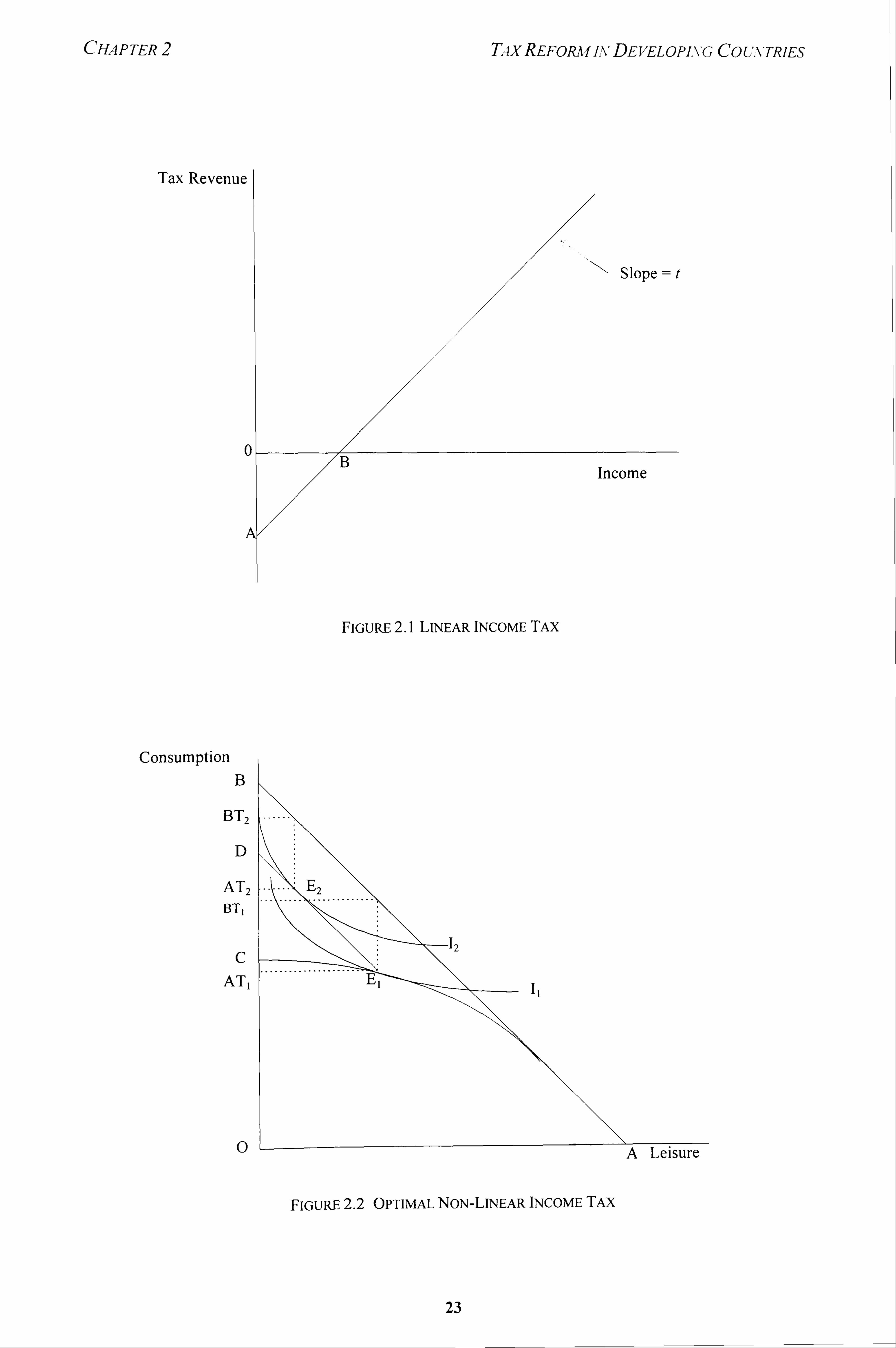
Figure 2.1 shows a linear income tax schedule where OA is the lump-sum payment (or

negative tax handout) and a constant rate of tax t is levied on income. The linear income

tax schedule is given by:

Tax revenue = -oc + tY

where -(x corresponds to the lump-sum payment, t is the marginal tax rate and Y is

income. The issue is to set the values for t and (x that would minimise the excess burden

associated with income redistribution. Higher value of t is associated with greater tax

progressiveness and larger excess burdens. The optimal linear income tax will be the

'best' combination of a and t that maximises social welfare subject to the constraint of

the required revenue to be raised. In his -discussion of models of optimum income

taxation, Stem (1976) suggests that social welfare is maximised when t= 19 per cent,

assuming that the elasticity of substitution between leisure and income is 0.6 and the

required government revenue is 20 per cent of income. He shows that a more elastic

labour supply is associated with a higher cost of redistribution, and hence the optimal

value of t is lower. In a society with extremely egalitarian objectives, where weights are

II Meade (1978) provides a discussion of such arrangements.

22

CHAPTER 2

Tax Revenuc

T4xREFoRmj, N'DEJ, 'ELOPI, \'G COUNTNES

FjGuRE 2.1 LINEAR INCOME TAX

Consumption B

BT2

D

AT2 BTI

C

AT,

0 A LeISUFC

FIGURE 2.2 OPTIMAL NON-LINEAR INCOME TAX

23

CHAPTER 2 Tix REFORA 1u DE lEL OPING CO UNTRIES

only assigned to the social welfare function of persons with minimum utility, Stern finds

that the maximum criterion for the marginal tax rate is about 80 per cent.

In the progressive income tax system, the marginal rate of tax varies with income. From an 'ability to pay' argument, the highest income earners pay the highest rates of taxation for the system to be 'fair'. However,, there are some disagreement with this

policy emerging from the literature on optimal non-linear taxation. Instead of taxing the highest marginal rate on the highest income earner, Seade (1977) argues that social

welfare is maximised when individuals at the very top of the income scale pay marginal tax rate of zero. Commenting on the UK income tax, Kay and King (1986: 214) note that

the marginal tax rates are high at the top as well as bottom levels of income, that is a U-

shaped schedule. Contrary to previously held belief, the principle that emerges is that

marginal tax rates should be low at both the highest and the lowest levels of income.

High marginal tax rates on the largest incomes bring in very little revenue and are not

worth pursuing if they have adverse consequences. On the other hand, the welfare

support for low income families comes to nothing if their receipts are taken away by high

marginal rates of tax.

It can be shown that even if the marginal tax rate of the higher income-earner is

brought to zero, this would not bring a loss of tax revenue for redistribution to the poor.

Figure 2.2 shows the optimal non-linear income tax. The budget line AB is the trade-off

between leisure and income before tax for the individual with the highest income. After

income tax, the budget line is a curvilinear AC. The individual maximises his income at

El where his indifference curve 11 touches the budget line. His after-tax income is AT,

and the tax revenue is (BTI-ATI). If the marginal tax rate is set to zero for income

earned above BT1, the budget line for this segment is given by EID, which is parallel to

AB. The budget line for the individual is now AEID. The new equilibrium for the

individual is E2, as he increases his work effort and earns up to BT2. The total tax paid

remains the same, i. e. (BT2-AT2) ý (BTI-ATI) but the individual is better off since he

has a higher after tax income of AT2and is on a higher indifference curve12. This implies

that the welfare of the top income-earner can either increase or be held constant without

the corresponding loss of welfare to others.

24

CH, -I P TER 2 T4. vREFORA f 1, N, DEVELOPIA'G COUNTRIES

2.5 Simplicity ofAdministration and Compliance

An important aspect often overlooked during attempts in reforming taxes is the improvement of the institutions governing tax administration and tax compliance. 12

According to Gillis (1989), most of the early post-war reforms focused primarily upon changing the tax structure alone,, which would be a sufficient condition for the failure of comprehensive, if not partial reforms. In reforming the tax system, it is necessary to keep

the system as simple as possible for effective implementation. This is especially the case

in developing countries given a lack of trained administrative personnel, resource limitations,, and a lack of accounting sophistication amongst taxpayers.

Voluntary compliance is central to taxation where the large mass of taxpayers

submit accurate reports of income and make timely payments of tax. Without voluntary

compliance, the scale and scope of problems may be more than what any tax agency can handle (Radian 1980). A complicated reform can generate serious implications on tax

administrators and taxpayers. The tax administration that requires high level of expertise

to absorb the new procedures would be depleted of its personnel. As the public demand

for more tax expertise to cope with the new procedures, the former tax administration

employees would sell their skills as private tax advisers (Radian and Sharkansky 1979).

In the case of Indonesia, the two proximate objectives of its tax reform which are

considered essential for obtaining the other tax goals are the drastic simplification of the

tax structure and the depersonalisation of tax administration. Before the reform, the

criteria for exemptions for small firms were complicated and tax officials had many

discretionary authorities to grant them. Hundreds of ad hoc amendments had been

adopted, which created a law that was incomprehensible to tax payers and tax collectors

alike. The tax system, which was used to serve numerous non-revenue goals, became

excessively complicated, replete with anomalies and vulnerable to corruption. The

adoption of transparent criteria and the reduction of frequent contact between tax

officials and tax payers reduce the scope of corruption in tax compliance and collection

(Gillis 1985). The tax simplification in Indonesia does not only mean having lower and

12 For an excellent and provocative discussion of the administrative dimension of taxation in developing countries. see Radian (1980).

25

CHAPTER T-1. vREFORA I I. %'DE VEL OPING CO UNTRIES

more unified tax rates, it also involves dismantling all kinds of tax incentives and broadening of the tax base.

According to the World Bank (1988), some approaches that can be adopted for

simplifying commodity taxes are: (a) shifting from the taxation of production to the

taxation of consumption and (b) shifting from the taxation of international trade to the

taxation of domestic transactions. Income taxes can be simplified by: (a) restructuring

company taxes so that average effective rates are high for revenue purposes and marginal

effective rate low for investment purposes, and (b) restructuring of personal taxes to

include all sources of income,, with lower maximum rates, fewer brackets, higher

exemptions, and the elimination of most existing special allowances.

3. APPROACHES To DEVELOPMENT TAXATION

After the Second World War, there are essentially two traditions influencing the design

to development tax policies. First is the interventionist tradition that believes that the

government could and should influence the achievement of a variety of policy objectives

through the tax system. Prominent analysts using this approach include Heller (1954),

Kaldor (1965), and Lewis (1966). The second is the reductionist tradition that argues the

government cannot achieve many of the intended policy goals and it should not try to do

so. The second approach, first advocated by Bauer (1957), is very much in the mould of

the classical economics tradition and is now gathering a wider appeal (Bird and Oldman

1990).

1 Optimal Tax Reform

Optimal taxation, which has been the subject of theoretical research in recent

decades , is very much linked with interventionism. Newbery and Stem (1987) explore

into the application and implications of the optimal tax approach for developing

countries. The optimal tax theory provides the foundation for sound empirical work by

sorting out 'the grammar of the argument' (Atkinson and Stiglitz 1980) and increasing

rigour and formalisation of the analysis (Bird and Oldman 1990). Ahmad and Stern

(1984,1986,1987) have examined questions such as the design and reform of indirect

taxation in terms of optimal taxation for India and Pakistan.

26

CHAP TER 2 T-i, vREFORA1 1, v DE VEL OPING CO UNTRIES

The central question in reforming a tax system is how best to raise additional

revenue, since the extra taxation would affect the pattern of incentives and costs for

different households and the productive system. The government has to consider how the

tax changes are to be enforced and at what cost. The goal of optimal commodity taxation is to raise revenue from taxes on goods with as little loss of household welfare as

possible.

The usefulness of the optimal approach to tax reform should be weighed against

the reservations expressed on some of the policy recommendations of the optimal tax

theory (Lindbeck 1987), the demands it makes on data requirements (Deaton 1987) and

its insufficient recognition of the administrative dimension of tax reform (Bird 1989).

Lindbeck provides three arguments against using optimum taxation as a basis for actual

policy advice both in developing as well as developed countries. Firstly, optimum

taxation formula captures very few types of mechanisms for adjustment by the individual

agents (such as a shift between leisure and work or the consumption of different

commodities), while in reality there are many other adjustment mechanisms for taxes.

Secondly, even to calculate a single type of adjustment mechanism would require the

optimum tax formula that relies on extremely special assumptions, such as identical

preferences of all individuals, and special forms of the production function, such as the

Cobb-Douglas functions. Thirdly, the calculations are very sensitive to alternative

specifications of the various functions and the statistical parameterisation and are,

therefore,, subject to arbitrary decisions.

In contrast to Ahmad and Stern, Lindbeck (1987) recommends the adoption of

uniform commodity taxes as the basis for the tax system, although selective taxes on

goods can be used where the supply and demand elasticities are very low and the goods

are consumed more by the rich than the poor (see also Cnossen 1978). The adoption of

uniform indirect taxes differs from the optimum tax theory in that the adjustment of tax

rates to differences in demand and supply elasticities would be an exception rather than

the rule, and the functioning of the political process is an essential consideration.

27

CHAPTER 2 T-ixREFORI f i, \, DEVELOPING COUNTRIES

3.2 Market-Oriented Reform

Lindbeck (1987) suggests that tax reform forms part of the overall effort of

adopting liberalisation policies and 'getting the prices right' so that the market (rather

than the government) is left to play the role of allocating resources. In many countries,

this would imply the reversal of existing policies such as reducing protectionism, freeing

interest rates, and removing tax disincentives to save, invest, and work. It is not clear

whether liberalisation would result in higher or lower levels of taxation. The reduction in

tariffs may call for new sources of tax revenue, while the uneven distribution of income

that arises from reliance on the market may require higher public budgets and taxes for

redistribution. On the other hand, liberalisation could lead to lower taxes with the

reduction of subsidies to enterprises, greater reliance on users' fees for various types of

public services, a reduction of public bureaucracy and higher efficiency in the public

sector. There could be increased incentive for private saving, thereby reducing the need

for public savings and substantial tax reduction.

3.2.1 Supply Side Economics

The adoption of liberalisation and market-oriented policies has now more or less

become the accepted conventional wisdom for economists. In the 1980s some

economists advocate market reforms under the guise of 'supply-side economics' which

was considered by some as the remedy for the economic problems of the eighties.

Supply-side economists believe that free markets, with few exceptions, allocate resources

most efficiently. While they accept the existence of pure public goods and some merit

goods, they argue that policy makers would not necessarily provide even these goods in

the optimum quantity or at the lowest possible costs.

The political philosophy underlying supply-side economics comes from the

writings of Downs (1957), Buchanan and Tullock (1969), Niskanen (1971), and Breton

(1974). These writers regard governments as essentially inefficient because of their lack

of market discipline, and the agents of government have personal objectives that differ

from the goals of society. Supply-side economists maintain those government regulations

that are aimed at protecting consumers and workers distort relative prices and should be

eliminated to improve resource allocation in the economy. Most welfare and entitlement

28

CM P TER 2 T-ix REFORA f i. v DEI, 'ELOPI,, \'G COUNTRIES

programmes as well as high personal income tax discourage work effort. The reduction of these distortions would encourage savings and production by allowing the economic incentives of a free market to work.

The basic propositions of supply-side economics are not new. In a sense, supply- side economics that emphasises the objective of efficient allocation of resources and the importance of negative substitution effects of government economic policies are beliefs

held in mainstream classical and neo-classical economics. The merits of adopting the

supply-side approach in development economics are discussed by Peter Bauer (Bauer

1957; Bauer and Yamey 1957) even before this approach was 'popularised' in the 1970s.

Gandhi (1987) notes that the difference of this 'new' approach is the conviction 13 by popular supply-side economists that a substantial reduction of tax burdens

, in

general, and the rates of income tax, in particular, will have significant effects on

stimulating output and growth rates. The great importance placed on nominal marginal income tax rates by supply-siders is a reaction to the traditional literature on taxation that

gives an overwhelming bias towards equity and the accentuation of the progressive

income tax systems in recent years. Popular supply-side economists claim that the

negative substitution effects of income taxes are extremely high. As summarised by

Feldstein (1986: 27) 14 a reduction in marginal income tax rates is believed to result in

'rapid growth, dramatic increases in tax revenue, a sharp rise in saving, and a relatively

painless reduction in inflation. ' The reduction in marginal income tax rates will lead to a

change in the economic behaviour of households and businesses in favour of work,

savings, and productive investments and against leisure, consumption, and unproductive

investment.

An excellent assessment of the relevance of the popular supply-side economics to

developing countries is given in Gandhi (1987). Generally, it was found that the tax

structures of most developing countries depend more on commodity taxes than on

13 Popular supply-side economics have caught the public attention since the mid-1970s and been the subject of major debate in the United States and other developed countries. Unlike the basic supply-side position of the classical and

neo-classical economists, proponents of popular supply-side economics made wide-ranging claims on the efficacy

of efficiency-enhancing government economic policies and income tax policies. The writers on popular supply-side

economics include Laffer and Seymour (1979), Meyer (1981), Bartlett (1982), Fink (1982). Hailstones (1982),

Roberts (1982,1984). Guilder (198 1), and Canto, Joines, and Laffer (1983).

14 He does not believe in what is perceived as rather extravagent claims of the popular supply-siders.

U'- 29 OF i

CHAPTER 2 T4. ic REFORA 1 L\, DE VEL OPING CO UXTRIES

income taxes. Very generous tax incentives and tax reliefs are given to encourage savings

and investment. The income taxes rates in these countries are much too low for the Laffer

curve to be relevant. For developing countries to reach their full growth potential, they

would need to go beyond the issues of marginal rates of income taxes, which are

maintained by popular supply-siders as being of key importance. They need to reform

their entire tax system to increase efficiency.

4. EXPERIENCE OF DEVELOPING COUNTRIES IN TAX REFORMS

In recent years, many developing countries have undertaken tax reforms that vary in

scope, context, substance, and timing. For some countries, the reforms set in place

effective and viable tax systems that survive for many years. A notable example is the

Japanese tax reform packages of 1949-50 that were based on the recommendations of a

team led by Carl Shoup. 15 For some other countries, the reforms were short-lived or

efforts had not proceeded beyond the proposal stage. The comprehensive reform effort in

Bolivia was aborted in 1976-77, while the expenditure taxes proposed for India and Sri

Lanka were discarded because of unsatisfactory performance.

4.1 Scope

Tax reforms can vary in breadth and scope. Many tax reforms, especially the early

post war reforms, are concerned with changes in tax structure, but this is not a sufficient

condition for successful reform in developing countries. There is a need to introduce

changes to the tax system to address problems with tax administration and tax

compliance. As noted by Gillis (1989), tax reform can be comprehensive in

encompassing most or all important revenue sources, or efforts can be partial by being

confined to one or two tax sources. ' 6

Among the very first countries to adopt a comprehensive post-war tax reform was

Japan (1949-5 0) which tried to rebuilt itself after the war (Shoup et al., 1949). The reform

package involved improving the entire tax system to make income taxation as the basic

15 Shoup had teamed up with Musgrave and organised innovative reform packages for Liberia, Venezuela (Shoup).

Colombia, Korea, Taiwan, and Bolivia (Musgrave).

16 Gillis ( 1989: 11) considers a tax reform to be partial if it involves one or two tax sources affecting less than maybe

a third of collections.

30

CHAPTER 2 T-i, ýý,

REFOR, ýf I. %, DEI'ELOPI. \'G COUNTRIES

source of revenue in Japan, raising the level of tax sophistication, and improving tax

administration (Pechman and Kaizuka 1976: 321). Indonesia enacted comprehensive tax

reforms in the mid- I 980s to the entire tax system that had become inordinately complex. Jamaica reformed its taxes to simplify the tax system and minimises the adverse effects

of incentives. Its complicated, narrowly based income tax was replaced with a broadly

based, single-rate tax (Bahl 1989). Several countries in Latin America drew up proposals for major tax reforms as well. They include Columbia, which was based on the proposals

of the classic Musgrave Report (Musgrave and Gillis 1971), Venezuela (Shoup 1959),

Chile (Harberger 1989), and Bolivia (Musgrave et al. 1981; Gillis, 1989). Other

countries that have attempted comprehensive tax reforms are Liberia (Shoup 1970). and

Pakistan (National Tax Reform Commission, 1986).

Instead of adopting comprehensive reform, countries may undertake tax

adjustments or reform their tax system partially by introducing one or two taxes to

replace the existing ones. India (Kaldor 1956) and Sri Lanka (Kaldor 1960; Jenkins

1989) attempted to introduce a direct tax on expenditure but the proposal was later

abandoned. Brazil (Shoup 1965) and Uruguay (Harberger 1989) were among the first to

introduce value-added taxes (VAT) extending through the retail level which was later

adopted in twenty other developing countries during 1970-86 (Casanegra 1986). Gillis

(1989) notes that virtually every developing country that has enacted sales tax reform 17 18

since 1965 has chosen either the retail type form of VAT or the manufacturer's VAT.

4.2 Context, Substance and Timing

Countries have adopted a variety of reforms to rectify weaknesses in the tax

system and meet certain goals, such as revenue, equity and resource allocation. Tax

reforms are often motivated by the need to raise revenue in order to meet increasing

public sector expenditure commitment or overcome a financial crisis. The partial reforms

in Colombia in 1965-66 and Peru in 1968 were motivated by a financial crisis, while

17 Used in practically all Western European nations. According to Gillis (1989), twenty countries switched from

cruder forms of sales tax to value-added taxes extending through the retail stage. These include Ecuador (1970),

Bolivia (1973); Chile, Costa Rica, and Argentina (1975); Honduras (1976). Korea and Panama (1977). Mexico

(1980)-, Peru, Nicaragua, and Haiti (1982). Guatemala (1983). Colombia, Dominican Republic, and Madagascar

(1984), Turkey (1985); Niger. Portugal, and Taiwan (1986).

18 Enacted in Colombia in 1966, Indonesia in 1984. and proposed for Pakistan in 1987 (Gillis, 1989).

31

CHAP TER 2 T4xREFORA, f I. %'DEI"ELOPIXG COUNTRIES

those adopted for Venezuela in 1958-59 and Colombia in 1968-70 were meant to raise revenue to finance new expenditure on education and health (Gillis, 1989). However.

revenue enhancement was not always the primary consideration. For instance, the post- war reform programmes for Japan did not place revenue enhancement high on the agenda. Japan was in a state of near ruin and the priority was the creation and operation of a sound tax system (Shoup 1949; 1989). The Indonesian reform was motivated by the

need to enhance the size and 'elasticity' of non-oil revenue. The policies are intended to be revenue neutral in the short run, although the simplification of the tax system is expected to increase the effectiveness of tax administration'and compliance and generate increased revenue in the long run (Gillis 1989). The Indonesian experience has shown that the circumstances of the country should be central in organising and carrying out the

tax reform. As a strategy for improving the acceptability and success of the tax reform, foreign consultants kept a low profile while domestic expertise and policy makers were involved from the beginning in the formulation of the reform package.

The earlier post war efforts at tax reforms in developing countries place great

emphasis on income distribution and progressivity of the tax system (see Kaldor 1956,

1960; Shoup, 195%, 1970; Musgrave and Gillis 1971). By mid-1970s there was growing

scepticism on the efficacy of taxes to bring about income redistribution. According to the

World Bank (1988) taxes in developing countries often fail badly in terms of horizontal

equity because of poor tax coverage and arbitrary enforcement. Some formal activities

may be captured by the tax net, but not the informal or hard-to-tax formal activities,

thereby undermining the system's credibility and the willingness of the taxpayer to

comply. The tax systems are also not successful in vertical equity despite the highly

progressive rate structures. The World Bank asserts that the role of taxes in promoting

equity lies more in the revenue that is raised for distributive spending, especially for

poverty alleviation, rather than the structure of taxation per se.

Tax provisions have traditionally been used by governments to guide private

firms and individuals either towards or away from particular investments and activities. 19

Among some of the countries that relied heavily upon tax incentives to promote growth

and development through the 1960s into the 1980s are Bolivia,, Brazil, Colombia, Ghana,

19 For surveys of tax incentives, see Shah and Toye (1978); Heller and Kauffman (1963), Lent ( 1967).

32

CHAPTER 2 T4, v REFORM IvDE FEL OPING CO L'ATRIES

Indonesia, Liberia, Jamaica, Malaysia, Nigeria, Pakistan, Singapore, Sri Lanka, Sudan, Venezuela, and Turkey (Gillis, 1989; Shah and Toye, 1978). There are at least four

strategies that can be used in subsidising investments through the granting of investment incentives: (a) subsidise all new firms or all new investments; (b) limit subsidies to all firms within a well-defined set of industries; (c) subsidise firms which meet a set of criteria; and (d) restrict subsidies to firms that would not invest without a subsidy (Usher 1977).

Despite the pervasive use of tax incentives, there have been few attempts to

evaluate the effectiveness of these incentives (Bird and Oldman 1990). The evidence of the effectiveness of incentives on investments in developing countries remains unclear. Shah and Toye (1978) conclude that 'their impact is either slight or unknown' and the

persistence of their use is influenced by political economy. According to Gillis (1989),

later reforms in the 1970s and 1980s have moved towards tax neutrality in view of the

scepticism of the efficacy of tax incentives. For instance, the Indonesian reform of 1983-

84 abolished all special tax incentive provisions, while the Bolivian reforms of 1986 and

the Jamaican reforms of 1986-87 were addressed toward 'getting prices right'. The

Bolivian reform shifted away from incentives and adopted a uniform rate of VAT with

no exemptions, while the Jamaican reform abolished 16 special purpose tax credits in the

personal income tax and curtailed company tax incentives for agricultural and industrial firms (Gillis 1989; Bahl 1989).

Timing for the adoption of tax reforms can be contemporaneous, phased or

successive. Governments that attempt to adopt all the reform provisions at once, in stages

or enact reform measures on a tax-by-tax basis over a period of time. For instance, the

tax reform in Colombia, the Republic of Korea, and Turkey was a long drawn out period,

while major changes in the tax system for Indonesia and Malawi were implemented

quickly. Gillis (1989) argues that there is an advantage of implementing comprehensive

tax reform contemporaneously since this reduces the danger of revenue dislocation and

neutralises the opposition from interest groups who might lose in one element of the tax

reform but gain in another. The disadvantage of contemporaneous reform is the short

time available to the tax administration to deal with the changes in tax laws and

administrative procedures.

33

CHA P TER 2 T-ix REFOJU f lxDE rEL OPING COUNTRIES

Colombia has had major tax reforms in 1953.1961,1974 and 1986, which suggest that tax reform is inherently neither a continuous nor a once for all process, but a

periodic one. Tax systems must change to accommodate fundamental changes in

economic and political environment of developing countries (World Bank 1988: Box

4.7).

5. LESSONS AND TRENDS

Despite the variety of reforms adopted in developing countries, some coherent themes

emerge about the current status of tax reforms and point to wards the future directions in

the coming years. A comprehensive discussion on the experiences of developing

countries at tax reform transpired at the Conference of Tax Policy in Developing

Countries organised by the World Bank. 20 Some common themes and important lessons

that emerged may be summarised as follows:

1. Using the VAT The VAT is the preferred instrument for most developing

countries because of its strengths in revenue enhancement, tax neutrality,

vertical equity and improving the collection of other taxes. From the

experiences of countries with VAT, the following points should be noted: (a)

pre-retail VATs are not worth adopting because of distortion and

administrative complexities; (b) all services, except health care, education,

social welfare, banking, and insurance, should be included in the base; (c)

rate differentiation should be minimised, although the poor should be

protected; (d) VAT is an ideal tax for large, integrated economies with

sophisticated production and distribution channels and is less suitable for

small, island-type economies with narrow manufacturing base and large

cross-border trade.

2. Broadening tax bases. The base of existing taxes should be broadened to

enhance revenue and improve the simplicity, neutrality, and equity of the tax

system. The lack of success in implementing tax reforms is due to selective

20 World Bank Conference on Tax policY in Developing Countries, held in Washington, D. C. . in March 1990. The

papers from this conference are published in the World Bank Econotnic Review, Volume 5 September 1991,

Number I

34

CHAPTER 2 T-ix REFORA 1 1. \'DE VEL OPLVG CO UXTRIES

and lax enforcement, ineffective tax administration, institutional and political difficulties in taxing agricultural incomes, and an overall disenchantment

with income taxes as revenue instruments in an evasion-prone environment.

Limiting special tax preference. The provision of special tax preferences

often drains the national treasury. The potential gains of these preferences

should be weighted against the potential losses in efficiency and revenue. While there is a role for investment incentives that can offset the corporate

tax distortion,, attract foreign investment, create employment, promote risk

sharing, and correct information asymmetries, the granting of some of these

incentives often depends on administrative discretion that discourages

potential investors, especially non-residents.

4. Taxation offinancial assets. Contrary to belief, Chamley (199 1) found that

the financial sector in many developing countries is heavily taxed if one

considers both explicit and implicit taxes. Implicit taxes include seigniorage,

reserve requirements, lending targets at non-market rates, interest ceilings

combined with inflation. Using a partial equilibrium framework, Chamley

argues that most of the incidence of the effective taxation of financial

institutions falls on deposits.

5. Distributional impact of taxation. Shah and Whalley (1991) argues that

developing countries have very different non-tax policies and regulatory

environments from industrial countries. When these features are taken into

account, they can yield significantly different tax incidence estimates

calculated on the assumptions about tax shifting that are used in studies of

developed countries.

6. Taxing multinationals. The design of tax reform must reflect initial conditions

at home and abroad since developing countries are not only constrained by

their own institutional settings but also by the tax structure in capital-

exporting countries. The taxation of multinationals by a developing country

should be examined in terms of the tax regime of the home country, tax

havens and conduit countries, and transfer pricing practices. Home country

35

CHAPTER T4. v REFORA 1 lý, \'DE VEL OPING CO UNTR1ES

taxes influence the user cost of capital, while foreign f irms in a typical host

country face substantial variations in the user cost of capital. The incentive to invest depends upon the effective marginal tax rate, which can differ from an

average tax rate concept. In their study of Mexico, Shah and Slemrod (1991)

conclude that foreign direct investment (FDI) in Mexico is sensitive to tax

regimes in Mexico and in the United States, to the credit status of

multinationals, to country credit ratings, and to the regulatory environment.

7. Iniproving credibility. The success of any tax reform depends on the

credibility of the tax regime. Establishing business confidence in the

credibility of the tax regime requires greater attention to preparation, analysis

of reforms, advance consultation, and provision of a reasonable period of

adjustment before implementation.

8. Co-ordinating tax reform. A co-ordinated reform ensures consistency of individual tax changes with the overall objectives, including revenue

enhancement, protection (through custom duties) and economic performance.

A reform on reducing tariffs should be accompanied by reform of other

indirect taxes to offset potential losses and public revenue.

9. Considering the political economy. Tax reform proposals must carefully

consider the institutional features and tax administration of each country.

When it is difficult to get politicians to commit to comprehensive reforms

with medium to long term benefits, having periodic, incremental reforms

may be a pragmatic strategy. Where tax evasion is pervasive and the earlier

tax preferences are restored after the initial tax reform as a result of political

pressure, broadening bases and lowering rates can lead to a tax 'deform'.

10. Quantitative tools for tax policy analysis. There is a scope for a quantitative

evaluation of the impact of changes in tax structures for economic and

political economic analysis. As illustration, Dahl and Mitra (1991) use the

applied general equilibrium analysis to address questions in tax policy for

Bangladesh, India, and China. They argue that the costliest element of

modelling is establishing a consistent data set and the cost should be weighed

36

CHAPTER 2 TA, vREFORAf L\, 'DET'ELOPL\'G COUNTRIES

against the gains from modelling in producing consistent recommendations for sound policy formulation.

11. Optimal Taxation. There is limited scope of adopting the optimal tax theory

for developing countries because the optimal commodity tax rule assumes

global knowledge of preferences both in the present period and intertemporally, the absence of other tax instruments, and the representative

consumer. Once these assumptions are relaxed, the usefulness of the Ramsey

Rule is less clear cut. The optimal tax theory can serve as a guide to designing

(optimal tax systems' only if it considers the technology of tax collection,

such as the feasibility of tax instruments and the cost of tax administration

and compliance (Slemrod, 1990).

12. Taxation of agricultural land. Skinner (1991) examines the possibility of

replacing distorting taxes on agriculture with land tax. He concludes that a

land tax is not necessarily a superior alternative to export taxes for raising

federal government revenue, while progressive tax rates on land holdings are

nearly impossible to administer. A land tax may be suitable for local

government financing though.

6. CONCLUSION

In discussing tax reform in developing countries, this chapter considers the taxation

theory, empirical evidence, and political and administrative realities that are required for

producing reform proposals that can be implemented successfully. Since the post-war

and especially during the 1980s, many developing countries have embarked on tax

reforms, which range from comprehensive to partial reforms. The accumulated

experience garnered from the reform efforts of a wide range of countries is instructive

and has shaped the way development taxation is now approached. This review provides

the context and sets the stage for discussions in the later chapters on reforming the

Malaysian tax system and its implications on the economy.

37

Chapter 3

ECONOMIC TRANSFORMATION AND FISCAL REFORM

1. INTRODUCTION

During the last twenty five years, Malaysia enjoyed rapid economic growth and high

standard of living despite experiencing two recessions in the last two decades. Its per

capita income rose faster than that of the developed countries and most resource-rich Latin American countries which shared similar economic structures. The country has a

good track record of sound economic management, high savings and investment, and low

inflation. It has successfully reduced poverty and made notable progress in restructuring

the society.

Although growth was rapid during the last twenty five years, the economy

experienced sharp fluctuations. In addition, it faced problems of poverty and disparities

among ethnic groups and regions. In response to changing domestic needs and external

circumstances, the Malaysian development policies during the last twenty five years had

shifted from one of fiscal activism to fiscal restraint, from an expansionary to a much

trimmer public sector, from the government acting as the 'spearhead' of development to

the private sector as the engine of growth. Despite the policy shifts, the country

maintained a high degree of consistency and effectiveness in policy formulation and

implementation. This had enabled Malaysia to overcome its problems and move ahead to

its next stage of development in a relatively short time.

This chapter provides an overview of Malaysia's economic performance as well

as economic management and fiscal policies since 1970. It gives a historical review of

the country's economic development and analyses the underlying reasons for embarking

on policy reforms. This discussion is aimed at providing the background and socio-

CHAPTER 3 Eco, %, oAilc TRANSFORAMTIONAND Fisc. 4L REFORAI

economic context for our analysis on the tax system, which will be pursued in the later

chapters. In the next section, we discuss the four phases in Malaysia's economic

transformation and accompanying development policies. The third section examines

public expenditure and revenue for the last twenty five years, while the fourth section discusses the policies for the nineties and their implications on fiscal policies.

2. ECONomic TRANSFORMATION

For analytical purpose, it may be useful to examine the Malaysian economy in terms of

four phases of business cycle and economic management policies. The first phase (1970

to 1979) is a period of high growth accompanied with the adoption of the New Economic

Policy. The second phase (1980 to 1984) saw economic boom amidst the spiralling of

public expenditure and debts that made it necessary for the country to re-orientate its

programmes and fiscal policies. In the third phase (1985 to 1986), the country

experienced the worst recession since independence. The fourth phase (1987 onwards)

marked the rapid turnaround in the economy that placed it on a path of high economic

growth.

2.1 Phase I High Growth With Equity (19 70- 79)

2.1.1 Adoption of the New Economic Policy

It would be useful to provide a brief background to the formulation of the New

Economic Policy that was to become the watershed in Malaysia's socioeconomic

policies. In the 1960s, Malaysia was one of the most prosperous Southeast Asian

countries, with an economic growth rate averaging 6 percent per year. It had just attained

independence and was resource rich, being the world's leading exporter of rubber and tin.

Despite economic success at the aggregate level, poverty was prevalent and disparities

among different segments of society were widening. The incidence of poverty was

disproportionately high among the Malays, whose per capita income was only half that

of the Chinese and two-thirds of the national average. Clearly, the benefits of economic

growth had not 'trickled down' as was believed by the fashionable development theories

at that time, and dissatisfaction of the people was lurking beneath the calm surface of

fragile communal stability. The inter-ethnic dissatisfaction was heightened by pre-

39

CHAPTER 3 EcONOMIC TP, 4, \SFOR. 1f. 4TioA,, 4. \, D Fisc, AL REFORM

election political campaigns of 1969 that touched on the raw nerves of racial sensitivities. These culminated in the outbreaks of racial conflicts in major towns of the peninsula during the aftermath of the national elections, a traumatic event known as 'May 13'.

This inter-ethnic violence sent shock waves down the country. Parliament was

suspended and a state of emergency was declared. The National Operations Council was

formed to govern the country. In 1971 the New Economic Policy (NEP) was formulated

and pronounced in the Second Malaysia Plan. I Since background papers on the

formulation of NEP are not available in the public domain, it is probably fair to say that

the policy makers realised that the communal riots represented an alarming fissure in the

Malaysian society, which was composed of three major races, each with its own

language and dialects, customs and traditions, religious beliefs, dietary preferences and

habits. Even occupations and locations were identified with race. There are ample

examples of societies with more homogenous characteristics which were torn apart by

years of political tension and conflict. For a society that was so differently constituted, it

became even more crucial for the situation to be handled with great care and foresight. If

handled well, the country could be on the road of national reconciliation. Even more, it

had every potential of becoming a vibrant, dynamic society, combining the strengths of

different ethnic groups and where the inter-ethnic differences could even become a

source of creative stimulation and enterprise. However, if handled badly, this would

result in a volatile cocktail that could lead to the disruption and eventual break-up of the

Malaysian nation.

Accordingly, national unity was elevated into the over-riding objective of

national development efforts. The strategies to achieve this national objective were two

pronged: poverty eradication and restructuring of society. This pronouncement was an

acknowledgement that certain affirmative actions were needed to redress the imbalances

in society. It was also a recognition that the pursuit of economic growth by itself was no

I The Malaysia Plans are medium-term five year development plans encompassing all aspects of

socioeconomic development of the country. Development expenditure allocations made at the start of

the plan are revised in the midterm review. Malaysia's development in the 1970s was covered by the

Second Malaysia Plan (1971-75) and the Third Malaysia Plan (1976-80), while developments in the

1980s was under the Fourth Malaysia Plan (1981-85) and the Fifth Malaysia Plan (1986-90). These four

plans were guided by the long term First Outline Perspective Plan (1971-90). The Sixth Malaysia Plan

(1991-95) and the Seventh Malaysia Plan (1996-2000) contain policies, strategies and programmes for

the nineties and are directed towards achieving the overall objectives of the Second Outline Perspective

Plan (1990-2000).

40

CHAPTER 3 EcoA'OAiic TR, 4ASFOR. lf4TIOA'AAD FISC4L REFORAf

longer considered to be adequate or sufficient in developmental terms. In 1971 Malaysia

decided that its economic growth must be coupled with equity. This was a substantial

advance of the policies of many developing countries where discussions were about 'trade-offs' between growth and equity (see Killick, 1983: 151-153). Later, the influential World Bank's study Redistribution With Growth (Chenery et al., 1974) called for a

paradigm shift in the approach to development. In the introduction of the book, Chenery

noted that despite a decade of rapid growth in underdeveloped countries during the

sixties, this growth had been very unequally distributed, thereby calling into question the

very idea of aggregate growth as a social objective.

Given the set of circumstances the policy was conceived and formulated, there

was a single-minded commitment at all levels of government in implementing the NEP

strategies, which was itself a basic ingredient for the policy's success. Many policies and

targets were set for this purpose, while special entries for poverty and restructuring

programmes were made for the allocation of public ftinds. The NEP also called for a

bigger pro-active role of government to rectify what might seem to be 'market failures'.

In the implementation of this policy, however, two provisos were made clear: 1) that no

segment of society should feel deprived in pursuit of distributional goals; and 2) that the

policies were to be implemented within the context of rapid economic growth.

The net result of NEP was a major improvement in the transformation of

Malaysian society. There was greater equality among different communities than ever

before and incidence of poverty was reduced to a low level. The wide ranging support by

voters from all communities for the ruling coalition party after two decades of NEP

implementation might be taken to be an indication of the support by the general

population for these policies. However, these policies also brought about the rapid

growth of the public sector, not only in general administration but also in commercial

and other activities. The issues of the inefficiency and poor performance of public

enterprises in most countries are well known since they had to fulfil a multiplicity of

potentially conflicting objectives (see Killick, 1983: 277-301). The problem of the rapid

growth of Malaysia's public sector was brought to a head barely one decade later when

the deterioration of budgetary deficits and recession necessitated a policy reversal to this

trend.

41

CHAP TER 3 ECONOAfic Tk4N'SFORAf A TIO, %'. A, \, D FISCAL REFORAf

2.1.2 Economic Performance

The Malaysian economy performed well during the seventies, with the exception

of the recession in 1975. Gross domestic product (GDP) grew at a sustained average rate

of 7.8 percent per annum, while per capital income rose to RM3,738 in 1980.2 Despite

experiencing economic fluctuations, the country registered rapid growth given its wealth

in natural resources, especially large reserves of arable land, as well as its successful

adoption of the export-oriented growth strategy, prudent economic and financial

management, and stable social and political institutions. During the seventies, the rubber

sector recorded sharp productivity increases, which cushioned the effects of steep price

declines. As part of diversifying the economy, palm oil production and the extraction of

timber expanded, while the country promoted the rapidly growing manufacturing sector

that was increasingly export-oriented.

As an open economy in which imports and exports each constituted about 50

percent of the GDP in 1971-80, the Malaysian economic performance faced the vagaries

of the world growth trend. The peaks and troughs in economic growth generally

correspond to movements in the terms of trade (see Figures 3.1 and 3.2). This pattern is

particularly apparent during the recessions in 1975 and 1985-86 as well as growth since

1976. There was a sharp increase in the terms of trade between 1975-79 when the prices

of crude oil, tin, palm oil, rubber, and sawlogs all rose simultaneously (Figures 3.3-3.5).

The past investments in oil palm cultivation in estates and land development schemes

contributed to the increased production and export of the crop. In value terms, the export

share of petroleum grew dramatically, up from 9 percent in 1975 to 17 percent in 1979.

During this period, the manufacturing sector grew at 11.3 percent per annum, while

manufactured exports rose by 25 percent per annum.

2 RM is 'Rinogit Malaysia', the Malaysian currency. As an indication, the exchange rate for fl. 00 was 11: ) RM5.30 in 1980 and RM3.92 in 1995.

42

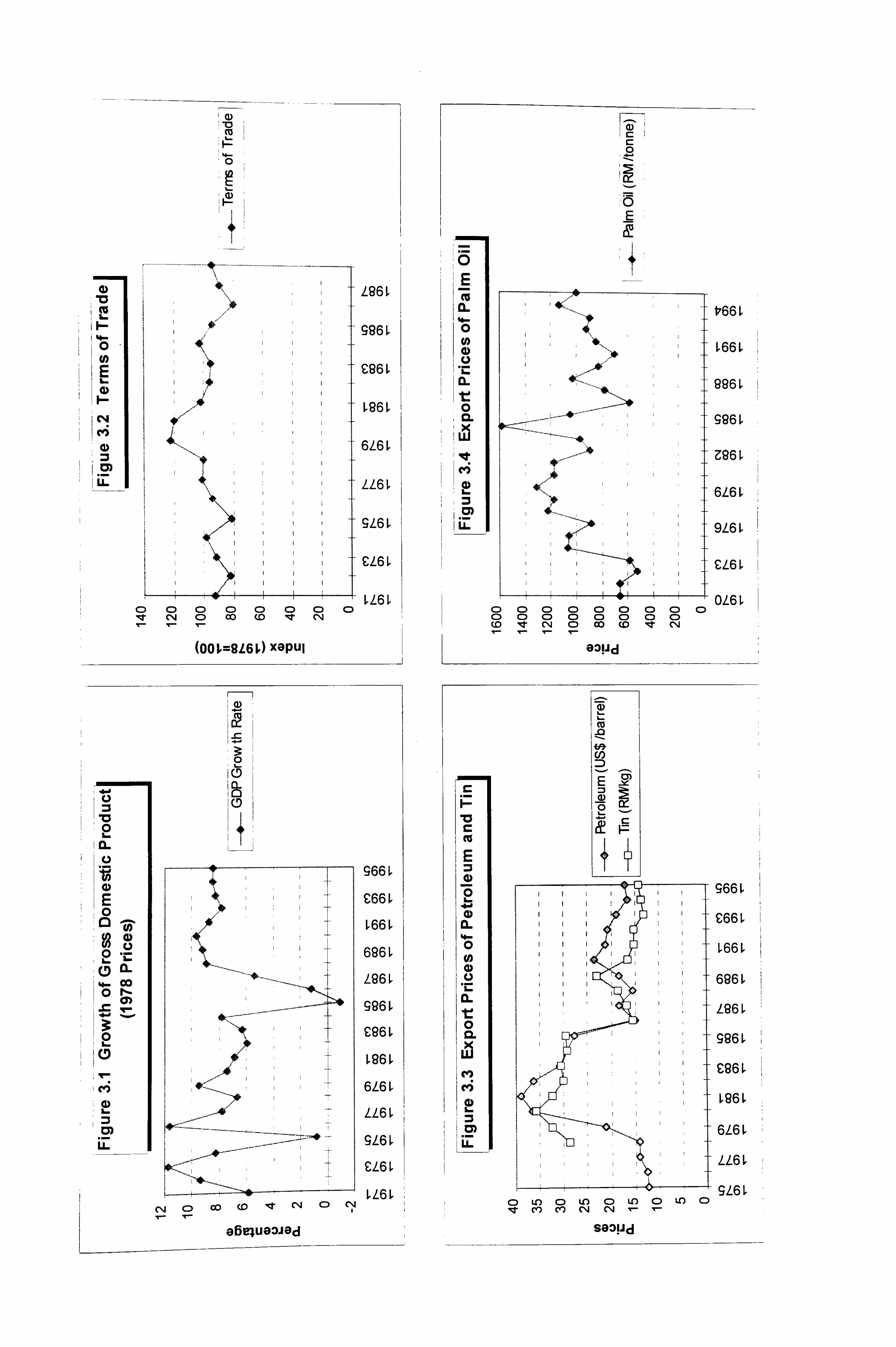
imý

4) lo

LL

6

L96 L

996 L

C86 L

ML

6L6 L

LL6 L

9L61

CL6 L

I Ir-I 1 bli-v bl ý CD 0 CD C: ) C: ) CD CD CD 1 le C, 4 CD OD (D le cli

(ook=BL6k)XGPUI

I CL C. )

II

cl)

0

0 E

CL

CL

Ul

ý, 0 16.

LL

t7661

ý66L

996 ý

996 ý

Z96 L

6L6 L

9L61

CL6

C: ) CD C: ) C: ) C: ) a c) 0 CD C) CD C) C) CD CD CD CD (D le C, 4 C) 00 (0 le cli

r_

P V

E

7F)

4) IL

0

4)

CL it 0 CL

6

CO) C-i

12

6d). U)

E

0 -

C66

L66L

696 L

L96 L

996 L

C96 L

L96L

6L6 L

LL6 L

9L6 L C) LO C) LO C) U-) 0 1.0 C) 114" V) CO CN CN r-- V--

SGOIJd

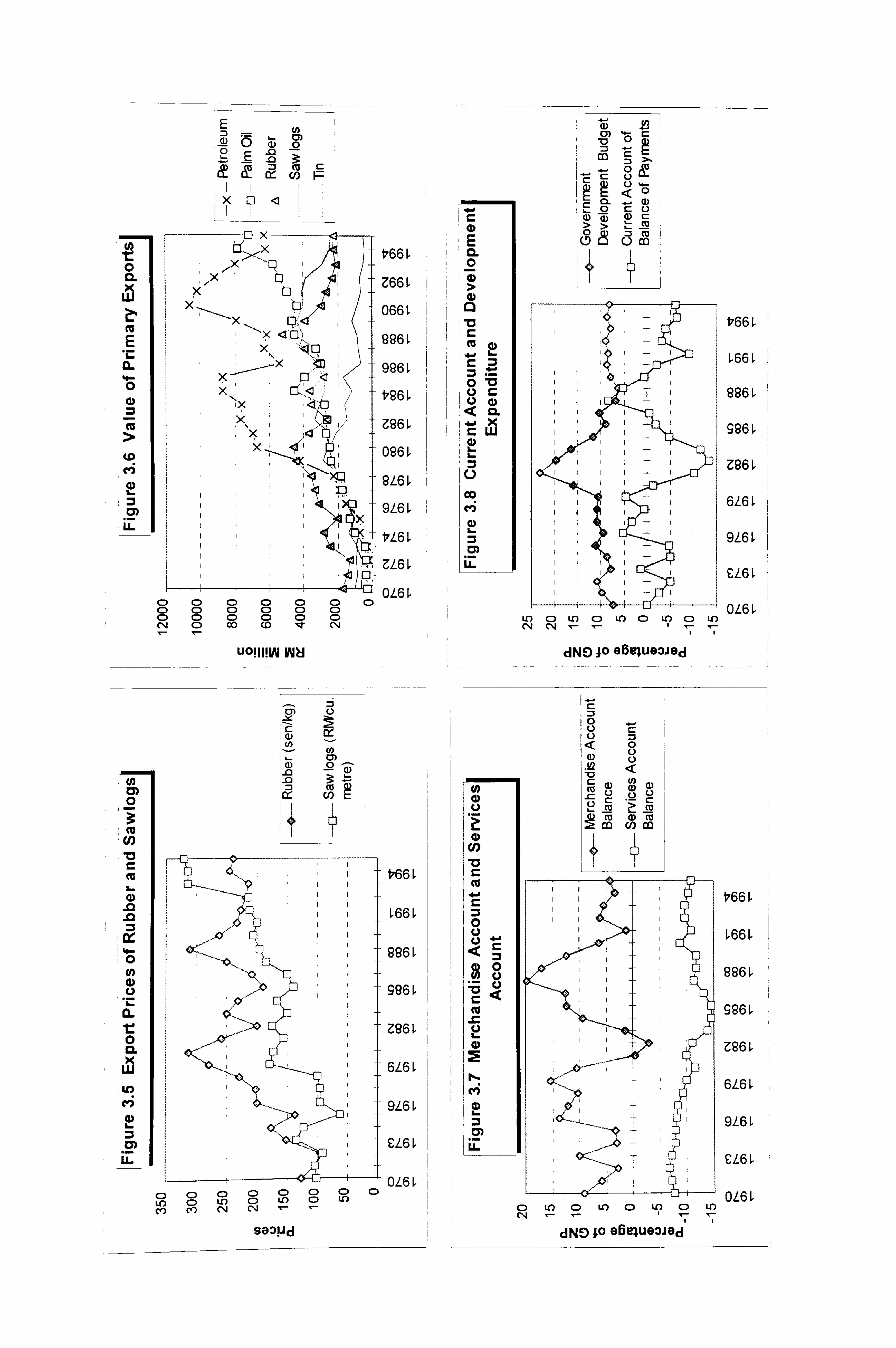
0 CL Lb

m E L. IL 4- 0

L-

ý0 cn 0

«a r_

4- 0

0 CL

Ul

E-

E =3 (L) 0

= o Q) U) 0) 0

1

01 m :3 m

x0

x t, 66 CL x0

Z66 > (D

066ý iIý !a

x <76y, 896 x

x 996ý 0M x tM

IX (D CL

Z86 Ul

(D L 0961

U61 X3 co AD 9 L6L co X--

VL6ý

ZL6ý

OL6 0 C) C) 00 C) C) C) C) C) C) 00 C) C) C) C) CN C) 00 co lq; r CN

UOIII! W INH

CO)

cu ?i

V661

ý66ý

996 ý

996 ý

Z96 L

6L6 ý

9L6 ý

CL6 ý

I OL6 C) C) C) C) 00 U*) C) Lf) C) U')

ce) C14 cli V-

SGOIJd

C, ) a) 0

a) Cl)

0 0

wo wo

.c 0 L. a)

H- C)

21 lu.

1. -

c 1 -0 0

M

o

<1 46

0c L) (D Wc > CU

t, 66

ý66ý

9961

996

Z961

6L6 ý

9L6 ý

Iýýý 0- CL6 L

OL6 L U') C) U') C) LO C) U') C) LO N CN

dND 10 8Be4uG3J8d

0

< 0

a) <

co (D L) cu - ffi a) (o m cn m

t, 66

ý66ý

886 ý

996 ý

Z86 ý

6L6 ý

9L6 ý

CL6 ý

OL6 L C) LO C) LO 0 LO C) LO N

dNE) 10 0614UOOJGd

CHAPTER EcONOMIC TRANSFORAIA TIOA'. -i, %D FISCA LR EFORA I

2.2 Phase H Boom With Growing Macro Imbalances (1980-84)

After the economic upswing in the late seventies, the Malaysian economy entered a new phase of its development in the 1980s. Its terms of trade 3 peaked towards the

middle of 1980 and then took a sharp decline that continued until 1986, with a brief

respite in 1984. The decline in the terms of trade was around 20 percent, while the slowdown in the international economic activities as a result of the recession in OECD

countries reduced the demand for Malaysian exports. On the supply side, the real growth

of important agricultural commodities, especially rubber and timber, had reached a

plateau, although this was compensated by increased exploitation of petroleum and

natural gas (Figure 3-6).

The declining terms of trade reduced the scope of private investment. The slowdown in demand, coupled with the decline in commodity prices, gave rise to a deterioration in the merchandise account and the current account of the balance of

payments (Figures 3.7-3.8). In response to the depressed external sector, the government

adopted an accelerated public investment and expenditure programme in 1980 and 1981

to boost economic activity and sustain real growth at a high level (Figure 3.9). While

some sectors were in the doldrums, employment in government services expanded

rapidly during 1980-82 (Figure 3.10). The counter-cyclical fiscal policy was in

anticipation of a rebound in petroleum prices and a quick recovery of OECD growth.

Although this sheltered the economy against the international recession, the temporary

relief was at a cost of an inflated current account deficit.

The strong growth in the domestic economy as a result of expansionary fiscal

policy and the tight labour market imposed pressure on the domestic price level. From an

inflation rate of 3.6 percent in 1979, consumer prices shot up and peaked at 9.7 percent in

1981 before falling rapidly to 0.4 percent in 1985 (Figure 3.11). The anti-inflation

measures include promotion of domestic savings and tightening conditions on

consumption credit. In addition, the government continued with the tight monetary

I Terms of trade index is calculated by dividing the export price index with the import price index.

45

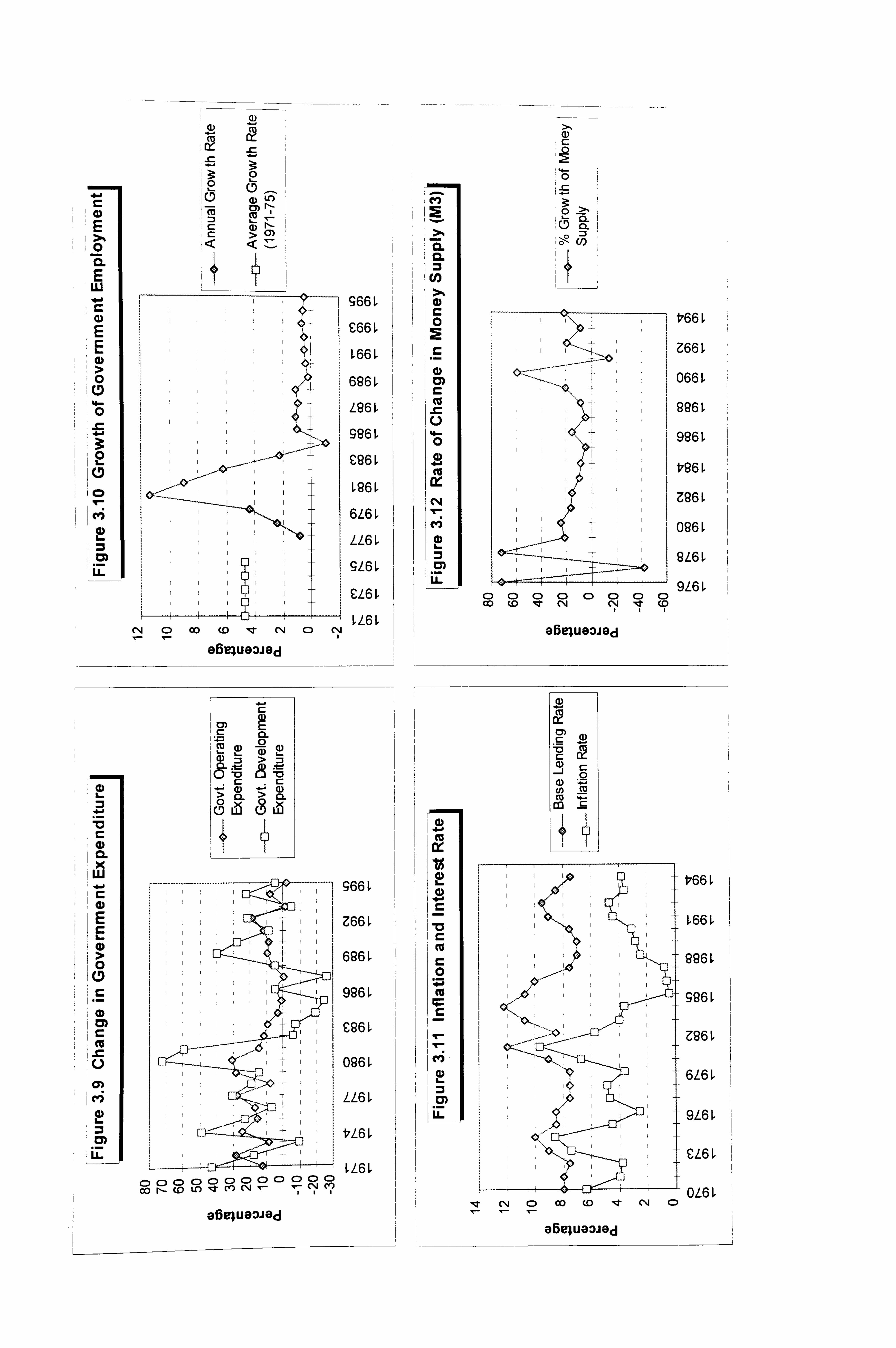
, 10 «a E w

E

ý jo

ýý en

: cm

: iz

ý10.

(D U') 75- CY)

cc

I C:

966 L

C66 L

L66L

696 L

L96 L

996 L

C96 L

L96L

6L6 L

LL6 L

9L6 L

CL6 L

LML C14 C) co co 'IT C14 C) CN

GrMU83JGd

CL M a) CD > :3 CL :R` 0 -0

Cl) Cl) > C)- > rL 00.

Lb

96 L iýIIII cc 11.

Z66

696

996

C96

0961

LL6

tL6 L

LL6ý C: ) C) C: ) C: ) C:: ) C: ) C: ) C) C) C) C) C) co r- (D Lo q- m 04 - -1 Cý C?

eBe4u83J8d

CL

co

0 Ez

a m

Ii 0) ý 11 ýI

CL ! ý (D 0- l :3'

CD CD CD C) C) CD C) CD OD (D lit clq (N 't (0

12

ý «a 1c i Co

CV)

5'

r 41)

t, 66 ý

Z66 L

066 L

996 L

986 L

V96 L

Z96 L

096 L

SL6 L

V66ý

ý66ý

986 L

T 996 L

Z86 ý

6L6 L

9L6 L

CL6 L

_J OL6 L , q- C, 4 C: ) co CD 14' CN C)

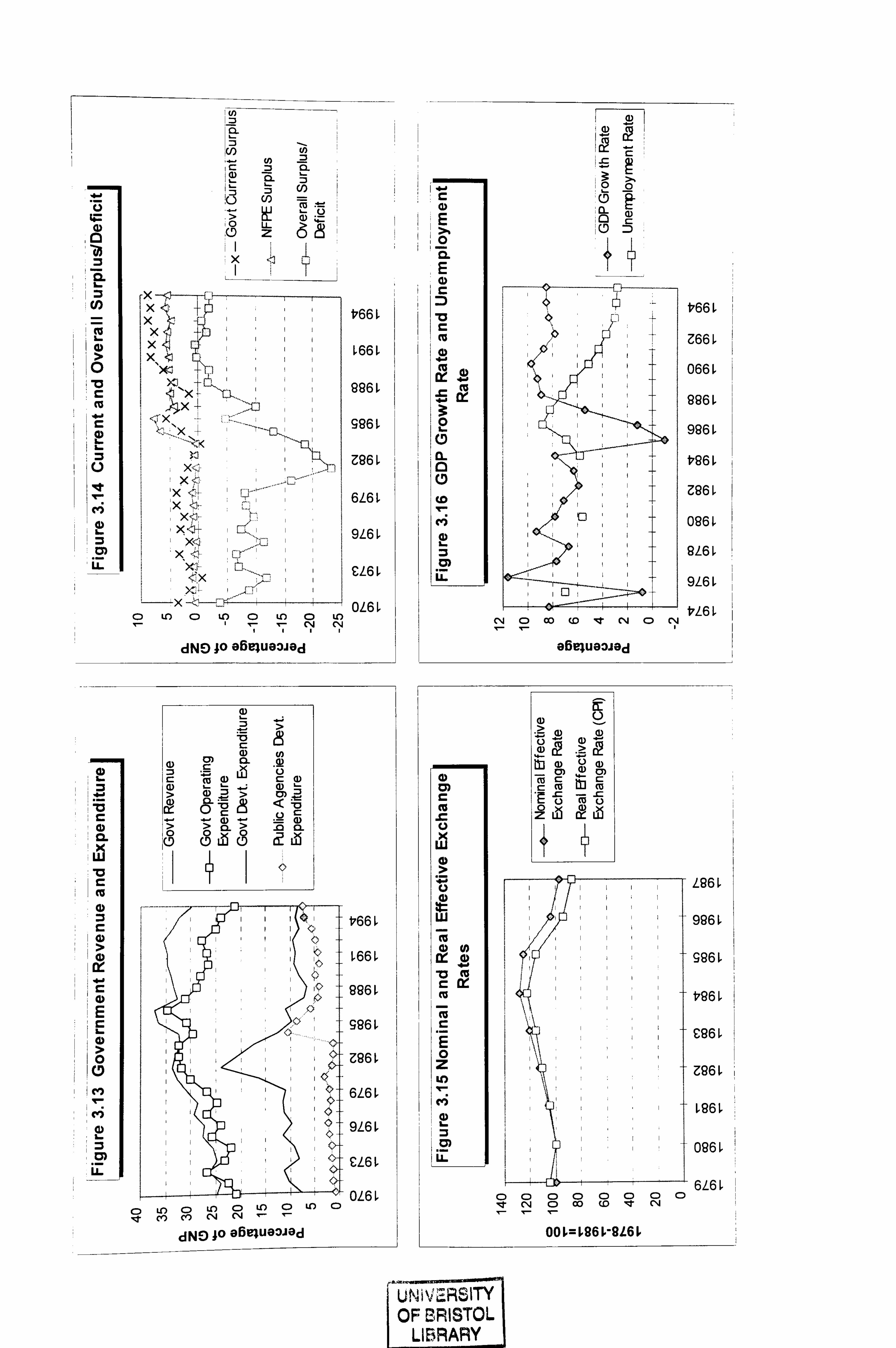
i U) M

ý Eý L- :3

[U)

c :3 CL

1 4.0 :3 (n I JI

sj L) >- (1) Z; '- 1 (D 0 LL

z

Cl) ix t, 66 IX x

> x x ý661

0 ' W ýj ý

ýC XI -11 i -x '.,., C: ýý IiI ! R96

986

Z96 x

x 6L6 L

9L6

CL61

OL6 ý U*) U') 0 Lr) a U')

T- T- II

Cý Cý

dNO 10 OBe4u83JGd

CL

Lb

C

(D 0 C

1 (D

r (D

E ý1 4)

> 0

LL

AD LD

C (D (D

Ad > <

0

CL 0 Lb

> 0 -0 CL

?L Lb

V66

ý66ý

886 L

996 L

Z96L

6Mý

iý 0-- Mý

iI

CL6 ý 0- <>- .. I OL6 ý

C) Ul) C) U-) C) U*) 0 LO C) M CO 04 04 --

dNO 10 GBeluG3JOd

=

CT

10 0

t'661

Z66 L

0661

996

9961

t, 86 ý

Z86 ý

086 ý

9L6 ý

9L61

VL6 L C*4 C) co (0 it N C) CN

oBinuGOJGd

a)

-c C. )

a) >

UNiV ir--- RES I TY OF BRISTOL

LIBRARY

(D

(D (152 (2

(D (D 0) 0) c C: cc (0

0 z Lb 12 Lb

CHAP TER 3 EcoN, w fic TR, 4,, NsFoRm, 4 Tjo, v .4 ýN, "D FISC. 4 LR EFORA f

stance adopted in the last few years to contain the inflationary effects from the second wave of oil price hike (Figure 3.12). Coupled with the expansion of aggregate demand, the tight monetary policy had the effect of pushing up interest rates with negative implications on investment and profitability in the tradable sectors. As shown in Figure 3.11 the base lending rate rose by 4.5 percentage points, from around 7.5 percent in 1979 to 12 percent in 1981 and again to 12.5 percent in 1984.

Already the processes of destabilisation were apparent when high growth rates

were sustained at the cost of inflation and growing current account deficit in the balance

of payments. The rapid expansion of the development expenditure by both the

government and non-financial public enterprises (NFPEs) during 1980-82 deepened the

overall budgetary deficit in the consolidated public sector financial accounts (Figures

3.13-3.14).

Demery and Demery (1992: 36-39) noted that the three main factors responsible for Malaysia's external imbalances over the period 1979-84 were the OECD recession

and the associated deterioration in the country's terms of trade, an expansionary fiscal

policy which caused a debt-induced interest rate shock, and an appreciation in the

nominal and real exchange rate. The income loss arising from the decline in the terms of

trade was considerable. As a percentage of GDP, the real income loss amounted to 7

percent in 1981 and 3 percent in 1982. However, the external imbalances could have

been avoided if this situation was accompanied by significant cuts in real expenditure

rather than the 'expenditure smoothing' behaviour on the part of the public and private

sectors. While pursuing an expansionary fiscal policy, there was monetary restraint

where lending to the public and private sector was curbed as part of the explicit anti-

inflationary policy. In Gan's study (1988) of exchange rates during the period of

destabilisation, he found that the inflow of external capital to finance the budget deficit

causes the appreciation of the nominal and real effective exchange rates (Table 3.1 and

Figure 3.15). This seriously eroded Malaysia's competitiveness in the world market,

dampened its exports of major commodities, and soon brought the country to a deep

recession.

48

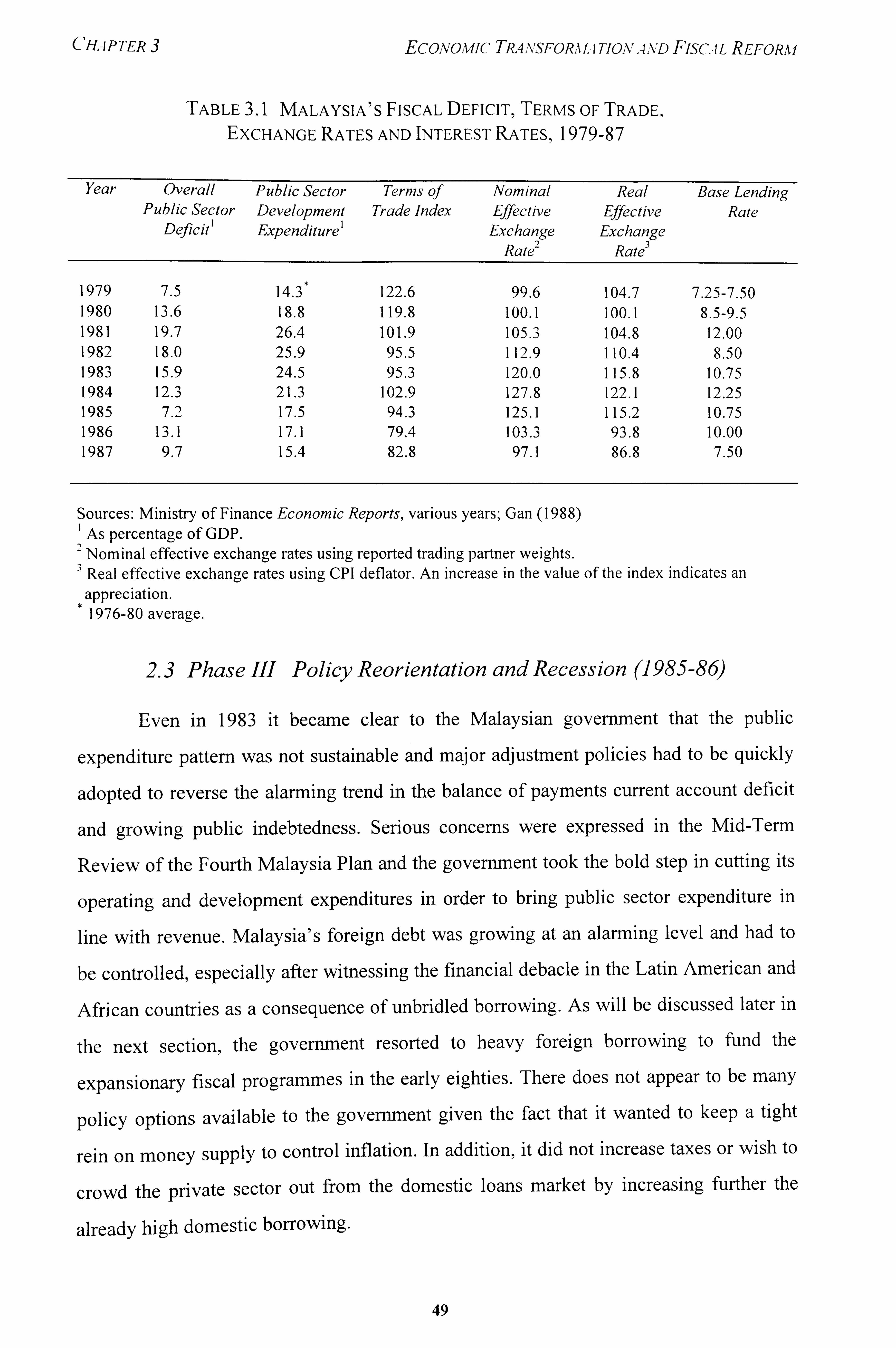
CH, -1 P TER 3 EcONOAfIc TP, 4ASFORA I. -I TIONAND Fisc.. ILR EFORA f

TABLE 3.1 MALAYSIA'S FISCAL DEFICITý TERMS OF TRADE, EXCHANGE RATES AND INTEREST RATES, 1979-87

Year Overall Public Sector

Deficit

Public Sector Development Expenditure'

Terms of Trade Index

Nominal Effective Exchange

Rate 2

Real Ef

. Tective

Exchange Rate 3

Base Lending Rate

1979 7.5 14.3) 122.6 99.6 104.7 7.25-7.50 1980 13.6 18.8 119.8 100.1 100.1 8.5-9.5 1981 19.7 26.4 101.9 105.3 3 104.8 12.00 1982 18.0 25.9 95.5 112.9 110.4 8.50 1983 15.9 24.5 95.3 120.0 115.8 10.75 1984 3 12. ) 21.3 102.9 127.8 122.1 12.25 1985 7.2 17.5 94.3 125.1 115.2 10.75 1986 13.1 17.1 79.4 103.3 3 93.8 10.00 1987 9.7 15.4 82.8 97.1 86.8 7.50

Sources: Ministry of Finance Economic Reports, various years; Gan (1988) 1 As percentage of GDP. 2 Nominal effective exchange rates using reported trading partner weights.

Real effective exchange rates using CPI deflator. An increase in the value of the index indicates an appreciation. 1976-80 average.

2.3 Phase III Policy Reorientation and Recession (1985-86)

Even in 1983 it became clear to the Malaysian government that the public

expenditure pattern was not sustainable and major adjustment policies had to be quickly

adopted to reverse the alarming trend in the balance of payments current account deficit

and growing public indebtedness. Serious concerns were expressed in the Mid-Term

Review of the Fourth Malaysia Plan and the government took the bold step in cutting its

operating and development expenditures in order to bring public sector expenditure in

line with revenue. Malaysia's foreign debt was growing at an alarming level and had to

be controlled, especially after witnessing the financial debacle in the Latin American and

African countries as a consequence of unbridled borrowing. As will be discussed later in

the next section, the government resorted to heavy foreign borrowing to fund the

expansionary fiscal programmes in the early eighties. There does not appear to be many

policy options available to the government given the fact that it wanted to keep a tight

rein on money supply to control inflation. In addition, it did not increase taxes or wish to

crowd the private sector out from the domestic loans market by increasing further the

already high domestic borrowing.

49

CHAPTER EcONOA, fIc TZ4 NSFORAIIA TION, 4,, NTD FisCA LR EFORA f

A reversal in the development approach was clearly needed to reduce the high fiscal deficit and related external borrowing requirement. The previous policy of fiscal

expansion and monetary restraint gave way to a policy of fiscal restraint and monetary

expansion. In addition, the real exchange rate was allowed to depreciate to restore the

competitiveness and profitability of the tradable sector. Wide ranging measures were

adopted in the Mid-Term Review of the Fourth Malaysia Plan to re-orientate public

policies and set the stage for a reduced role of government in development after the mid-

eighties. This proved to be the next milestone in Malaysia's development thrust after the

adoption of NEP in 1971. These policies were adopted in 1984 and continued to be

implemented even during the recession period in 1985-86. The budget restraint was

applied without resorting to counter-cyclical policies that could stimulate the economy from the demand side. While limiting the expansion of the public sector, the government

sought to revitalise the economy from the supply side by removing what were perceived

as the factors constraining economic growth.

From the national accounts identity, Demery and Demery (1991: 53) examined

the overall pattern of expenditure changes which brought about the initial destabilisation

and the subsequent adjustment in Malaysia. The decomposition of the observed changes

in the trade balance into the various expenditure components are shown in Table 3.2.

During the phase of rapid fiscal expansion in 1979-82, public consumption and

particularly public investment contributed the main bulk of the expansion in absorption

and accounted for 98 percent of the change in the trade balance as a ratio of GDP. The

situation was different during 1982-87 when the trade deficit was narrowing. During this

period, the burden of expenditure change was more evenly spread, with private

consumption being most important component. As noted by Demery and Demery,

reductions in expenditure during the adjustment phase were principally borne by the

private sector (66 percent), in direct contrast to the expansionary and destabilisation

phase.

50

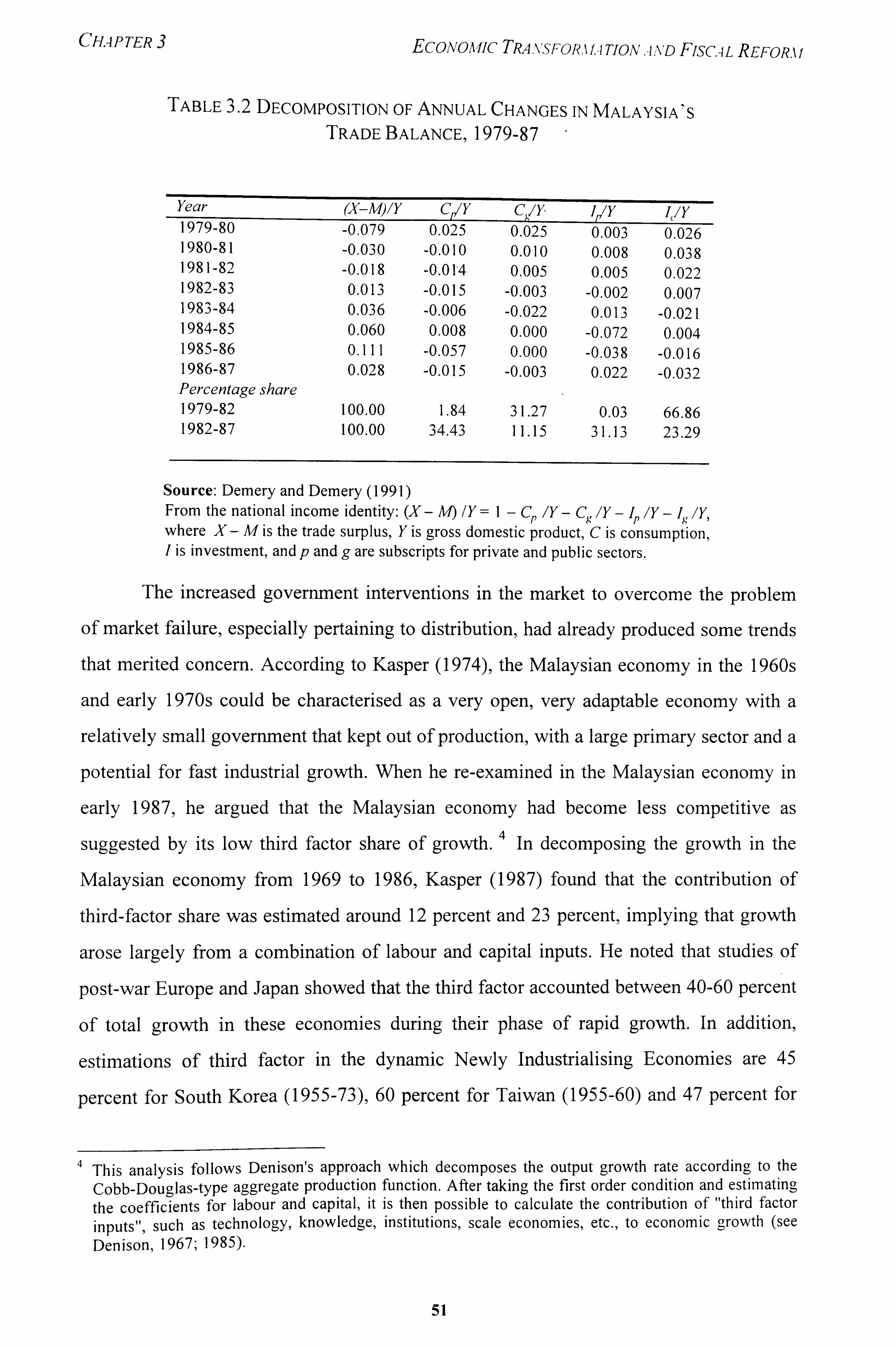
CHAPTER 3 EcONOAlIc TRANSFORI f. -I TIONA AD Fisc. 4 L REFORA f

TABLE 3.2 DECOMPOSITION OF ANNUAL CHANGES IN MALAYSIA'S TRADE BALANCE, 1979-87 -

Year (X-Al)/Y CI/Y Cý, /y ip/y I, /Y 1979-80 -0.079 0.025 0.025 0.003 0.026 1980-81 -0.030 -0.010 0.010 0.008 0.038 1981-82 -0.018 -0.014 0.005 0.005 0.022 1982-83 0.013 -0.015 -0.003 -0.002 0.007 1983) -84 0.036 -0.006 -0.022 0.013) -0.021 1984-85 0.060 0.008 0.000 -0.072 0.004 1985-86 0.111 -0.057 0.000 -0.038 -0.016 1986-87 0.028 -0.015 -0.003 0.022 "' 2 -0.01 Percentage share 1979-82 100.00 1.84 31.27 0.03 66.86 1982-87 100.00 34.43 11.15 31.13 23.29

Source: Demery and Demery (199 1) From the national income identity: (X - M) 1Y =I- CP 1Y - Cýý 1Y - IP 1Y - Iýý 1Y, where X-M is the trade surplus, Y is gross domestic product, C is consumption, I is investment, and p and g are subscripts for private and public sectors.

The increased government interventions in the market to overcome the problem

of market failure, especially pertaining to distribution, had already produced some trends

that merited concern. According to Kasper (1974), the Malaysian economy in the 1960s

and early 1970s could be characterised as a very open, very adaptable economy with a

relatively small government that kept out of production, with a large primary sector and a

potential for fast industrial growth. When he re-examined in the Malaysian economy in

early 1987, he argued that the Malaysian economy had become less competitive as 4 suggested by its low third factor share of growth . In decomposing the growth in the

Malaysian economy from 1969 to 1986, Kasper (1987) found that the contribution of

third-factor share was estimated around 12 percent and 23 percent, implying that growth

arose largely from a combination of labour and capital inputs. He noted that studies of

post-war Europe and Japan showed that the third factor accounted between 40-60 percent

of total growth in these economies during their phase of rapid growth. In addition,

estimations of third factor in the dynamic Newly Industrialising Economies are 45

percent for South Korea (1955-73), 60 percent for Taiwan (1955-60) and 47 percent for

This analysis follows Denison's approach which decomposes the output growth rate according to the Cobb-Douglas-type aggregate production function. After taking the first order condition and estimatina 2-=) 1_-:, 'In the coefficients for labour and capital, it is then possible to calculate the contribution of "third factor

inputs", such as technology, knowledge, institutions, scale economies, etc., to economic growth (see Denison, 1967; 1985).

51

CHA P TER ECONOxf1c TRANSFORMATION'AYD FISCAL REFORM

Hong Kong (1960-70) (Chenery, 1986: 21-22). The low third factor estimate for Malaysia implied low growth of labour and capital productivity and high incremental capital- output ratio (ICOR), raising questions about the quality of technology and innovation,

entrepreneurship, as well as policy and institutional framework. He argued that when governments intervene in markets, entrepreneurial energies are directed away from

genuine economic enterprise towards rentier profiteering that could cause the markets to lose structural flexibility. Kasper's study, which was undertaken just after the period of macro destabilisation and adjustment, painted a rather dismal picture of the Malaysian

political economy. His estimate of the third factor share in Malaysia's economic growth is biased downwards because it included the cost of large investment projects made in the early eighties but not their forthcoming benefits in contributing to economic growth

after the gestation period. Investment projects, such as the Heavy Industries Corporation

of Malaysia (HICOM), the liquefaction plant in Bintulu, purchase of LNG tankers, and

expansion of port facilities in Labuan, initiated in the early eighties had long gestation

periods and the benefits of which would only arise after the period of his study. While

one can dispute over the quantitative aspects of his estimates, the general tenor of his

arguments on the dangers of too much government intervention in the economy would

still be relevant.

To redress the structural problems, the government introduced economic

liberalisation and deregulation which improved the investment policies and incentives to

promote private sector participation. This appeared to be an important change from the

previous policy stance of increased public sector intervention which led to 'big

government'. Real public sector consumption and investments generally grew faster than

that for the private sector throughout the seventies to the early eighties. The exception

was during 1978-79 when private sector consumption and investment were buoyant with

the high prices of primary produce, the windfall earnings from petroleum and gas, and a

robust expansion of money supply. The Mid-Term Review of the Fourth Malaysia Plan

(Malaysia, 1984) and the Fifth Malaysia Plan (Malaysia, 1986) expressed the Malaysian

government's intention to make every effort in ensuring that growth was private sector

led, while the role of the public sector was to facilitate and promote a conducive

environment for economic growth and efficiency. Instead of competing with the private

52

CH. -IPTER EcONOA, fIc TP, 4 NSFORA M TIOA',, 4, NID Fisc. 4 L REFORAI

sector, the public sector was to complement private sector efforts. To quote the Fifth

Malaysia Plan (Malaysia, 1986: 4), 'The public sector will no longer play an

expansionary role in spearheading economic growth. It will, however, continue to

provide leadership through its efforts in creating a more suitable environment and

climate in which the private sector can play an enhanced role of generating growth ...

Among some of the policy measures to redress the structural economic problems

include:

1) Greater emphasis on management and financial prudence in the public sector

to reduce wastage and improve efficiency;

2) Privatisation programme of public enterprises such as Telekom, Malaysian

Shipping Corporation and the Kelang Container Terminal, and the

programme of Build-Operate-Transfer for highways and water supply; and

3) Relaxation of several NEP guidelines and legislative measures, such as the

Industrial Coordination Act of 1975 and the Companies Amendments Bill,

1984, which were earlier adopted to facilitate the restructuring process but

were later regarded as constraining private sector investment.

Some other important policy measures adopted to release the supply side potential of the

economy were:

1) Industrial Master Plan (IMP) in 1985 which provided the strategies for the

rapid expansion of industries;

2) National Agricultural Policy (NAP) in 1984 aimed at income maximisation

and increasing greater productivity, efficiency and competitiveness in the

sector;

3) 'Look East' policy, for Malaysians to emulate the work ethics, attitudes and

management practices of successful Far East nations; and

4) 'Malaysia Incorporated' concept to forge a working partnership between the

public and private sector in promoting a dynamic and prosperous business

environment.

53

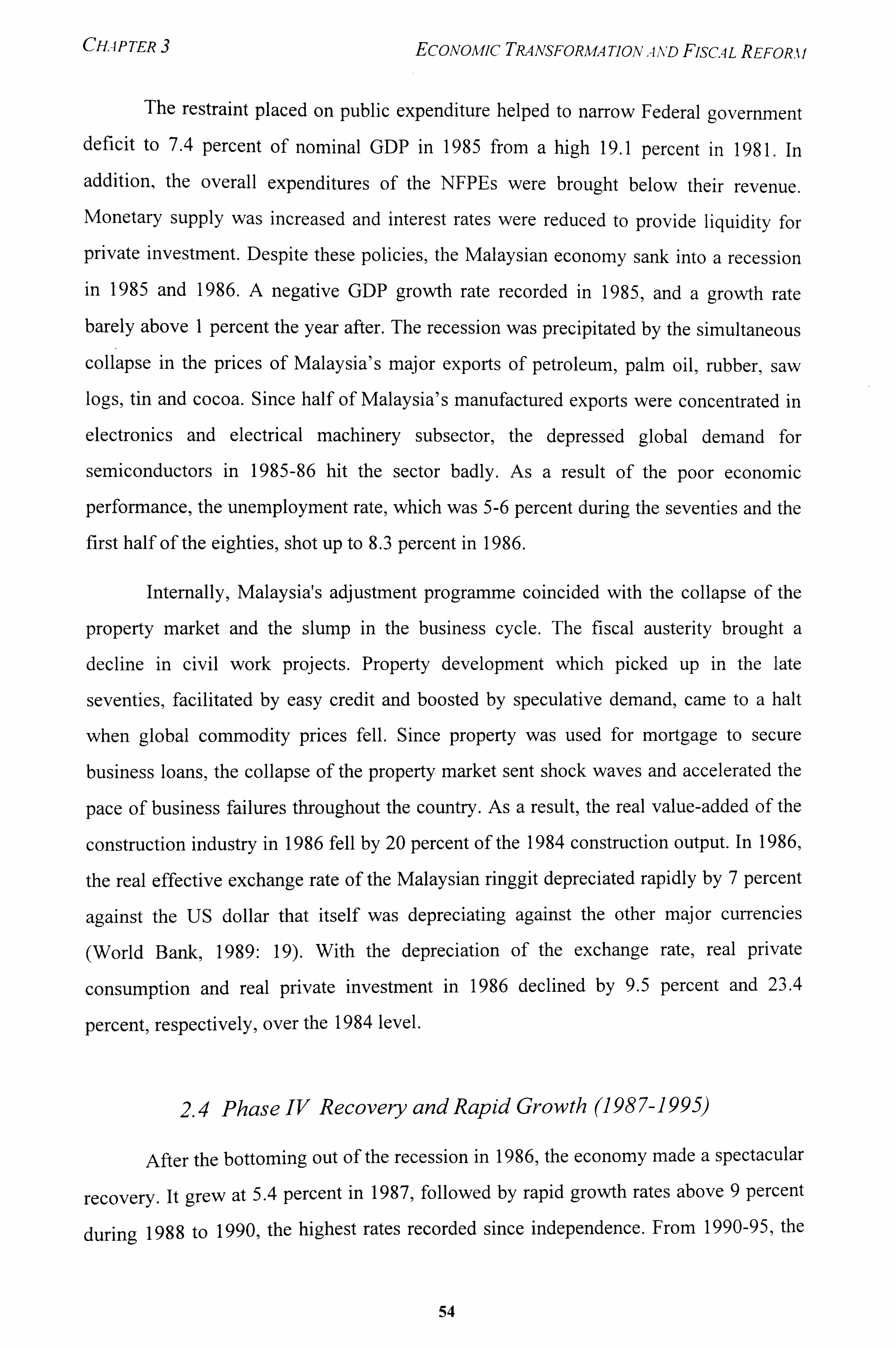
CHAPTER EcONomic TRANSFORMATION A AD FJsCA L REFOR. 1 I

The restraint placed on public expenditure helped to narrow Federal government deficit to 7.4 percent of nominal GDP in 1985 from a high 19.1 percent in 198 1. In

addition, the overall expenditures of the NFPEs were brought below their revenue. Monetary supply was increased and interest rates were reduced to provide liquidity for

private investment. Despite these policies, the Malaysian economy sank into a recession in 1985 and 1986. A negative GDP growth rate recorded in 1985, and a growth rate barely above I percent the year after. The recession was precipitated by the simultaneous

Coll apse in the prices of Malaysia's major exports of petroleum, palm oil, rubber, saw logs, tin and cocoa. Since half of Malaysia's manufactured exports were concentrated in

electronics and electrical machinery subsector, the depressed global demand for

semiconductors in 1985-86 hit the sector badly. As a result of the poor economic

performance, the unemployment rate, which was 5-6 percent during the seventies and the

first half of the eighties, shot up to 8.3 percent in 1986.

Internally, Malaysia's adjustment programme coincided with the collapse of the

property market and the slump in the business cycle. The fiscal austerity brought a

decline in civil work projects. Property development which picked up in the late

seventies, facilitated by easy credit and boosted by speculative demand, came to a halt

when global commodity prices fell. Since property was used for mortgage to secure

business loans, the collapse of the property market sent shock waves and accelerated the

pace of business failures throughout the country. As a result, the real value-added of the

construction industry in 1986 fell by 20 percent of the 1984 construction output. In 1986,

the real effective exchange rate of the Malaysian ringgit depreciated rapidly by 7 percent

against the US dollar that itself was depreciating against the other major currencies

(World Bank, 1989: 19). With the depreciation of the exchange rate, real private

consumption and real private investment in 1986 declined by 9.5 percent and 23.4

percent, respectively, over the 1984 level.

2.4 Phase IV Recovery and Rapid Growth (198 7-1995)

After the bottoming out of the recession in 1986, the economy made a spectacular

recovery. It grew at 5.4 percent in 1987, followed by rapid growth rates above 9 percent

during 1988 to 1990, the highest rates recorded since independence. From 1990-95, the

54

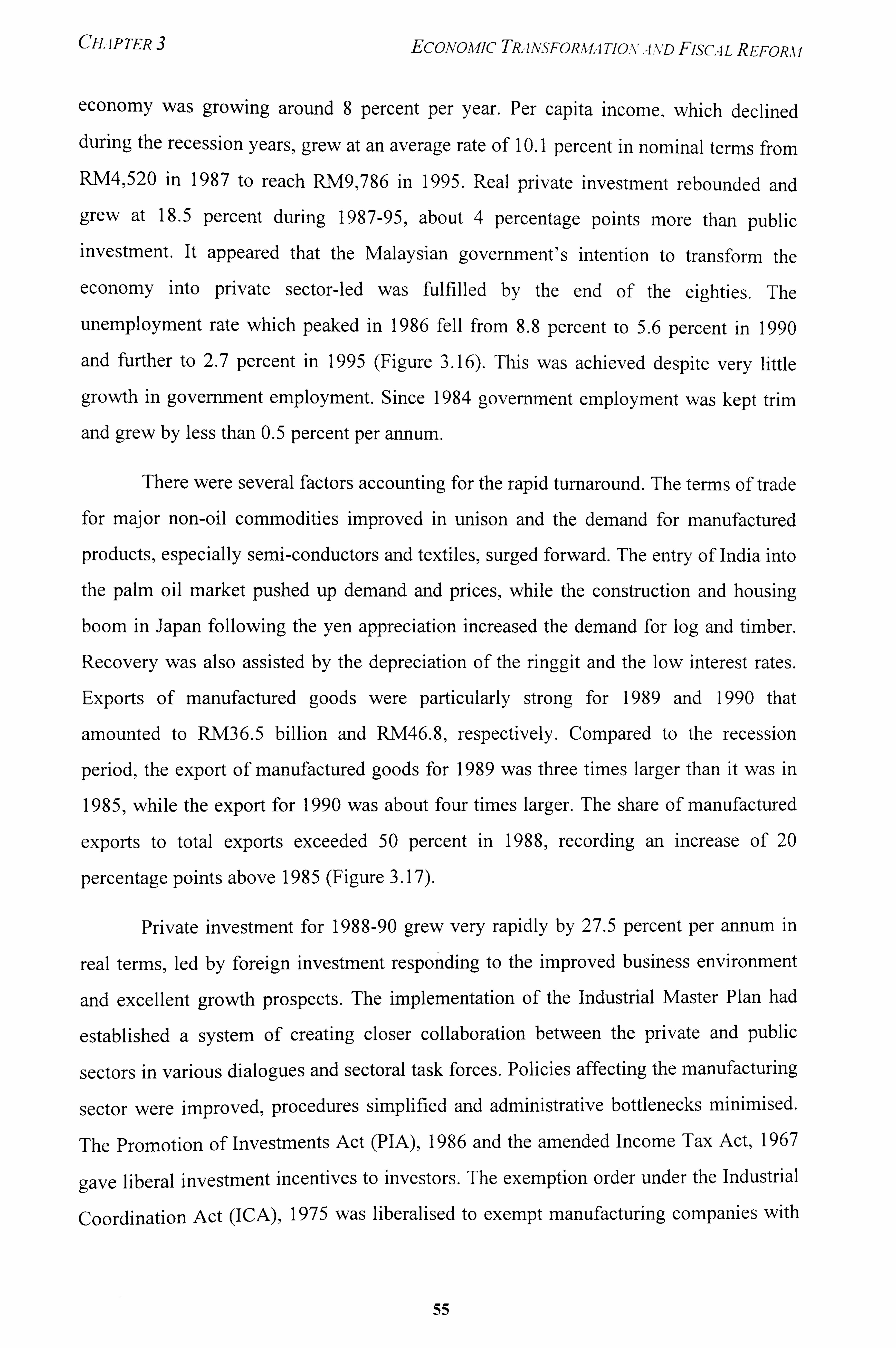
CHAPTER EcONOMIC TR, -i NSFORMA TIONAND FISCA LR EFORA f

economy was growing around 8 percent per year. Per capita income, which declined

during the recession years, grew at an average rate of 10.1 percent in nominal terms from

RM4,520 in 1987 to reach RM9,786 in 1995. Real private investment rebounded and grew at 18.5 percent during 1987-95, about 4 percentage points more than public investment. It appeared that the Malaysian government's intention to transform the

economy into private sector-led was fulfilled by the end of the eighties. The

unemployment rate which peaked in 1986 fell from 8.8 percent to 5.6 percent in 1990

and further to 2.7 percent in 1995 (Figure 3.16). This was achieved despite very little

growth in government employment. Since 1984 government employment was kept trim

and grew by less than 0.5 percent per annum.

There were several factors accounting for the rapid turnaround. The terms of trade

for major non-oil commodities improved in unison and the demand for manufactured

products, especially semi-conductors and textiles, surged forward. The entry of India into

the palm oil market pushed up demand and prices, while the construction and housing

boom in Japan following the yen appreciation increased the demand for log and timber.

Recovery was also assisted by the depreciation of the ringgit and the low interest rates.

Exports of manufactured goods were particularly strong for 1989 and 1990 that

amounted to RN436.5 billion and RM46.8, respectively. Compared to the recession

period, the export of manufactured goods for 1989 was three times larger than it was in

1985, while the export for 1990 was about four times larger. The share of manufactured

exports to total exports exceeded 50 percent in 1988, recording an increase of 20

percentage points above 1985 (Figure 3.17).

Private investment for 1988-90 grew very rapidly by 27.5 percent per annum in

real terms, led by foreign investment responding to the improved business environment

and excellent growth prospects. The implementation of the Industrial Master Plan had

established a system of creating closer collaboration between the private and public

sectors in various dialogues and sectoral task forces. Policies affecting the manufacturing

sector were improved, procedures simplified and administrative bottlenecks minimised.

The Promotion of Investments Act (PIA), 1986 and the amended Income Tax Act, 1967

gave liberal investment incentives to investors. The exemption order under the Industrial

Coordination Act (ICA), 1975 was liberalised to exempt manufacturing companies with

55

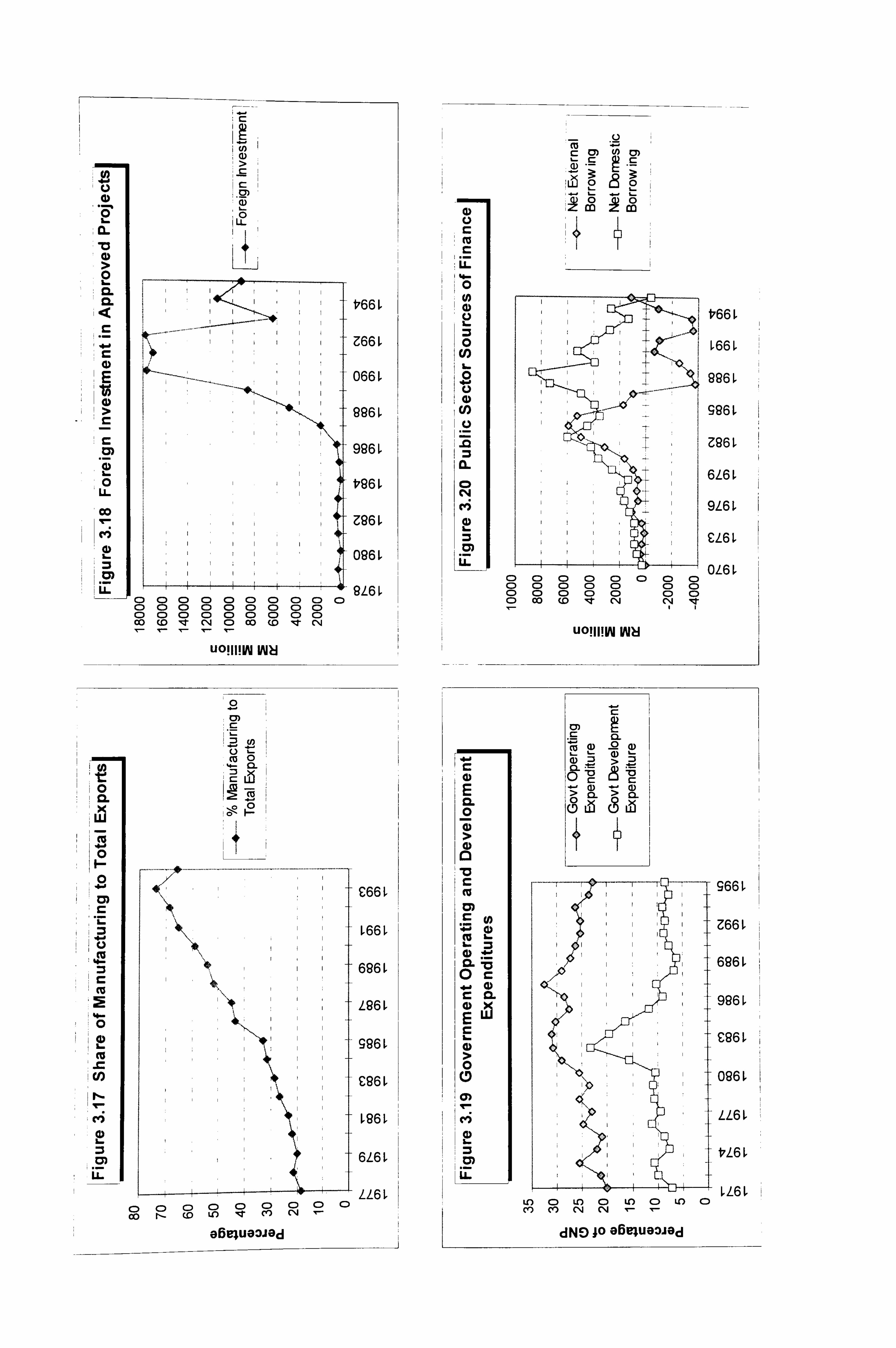
U)

�a) > U)

16. CL

0 L. CL CL

r_

m

0 U-

Co

1 LL

i0

t, 661

Z66

066[

996

926

V961

Z961

096

9L6 C) C) C) 0 C) C) C) C) C) C) C) C) 00 C) C) C) C) C) C) C) CC) (D C) CD CD C) CD C) C) CN C) co (D 14T CN

UOIII! W WN

io ýý0.

cm

LL

0 c7)

m0 4- 0-

76

C66 ý

166 L

6961

L861

996 ý

C961

186 L

6L6 ý

LL6 L Cý C) C) C) C) 0 C) C) a 00 r-- (D U-) lq; r cr) 04

GB14U83J8d

10

U) 0

(D U)

CD N C-i (D

-U.

E CL 0

(D

1.0

CL 0

CD

Lb E C

0

- 4-

C 0) U) 0) '-C C

Pu a +

.9 0- Co (D -9 (D

>

CL > 0-

Lb Lb

966 ý

Z66

6861

926 ý

C96 ý

096 ý

LL6 L

VL6 L

U') C) U") C) Lr) C) U") C) CIO CIO CN CN T. -

dNO 10 OBBIU03.10d

CHAPTER EcONOA fiC Tit4,, N'SFORl 1.4 TIONAAD FISCA L REFORA f

owners equity of less than RM2.5 million or 75 workers from being licensed. The equity

guidelines for foreign investment were liberalised. The cost of energy was reduced since March 1989 while the government introduced special rebate schemes for rubber and

textiles subsectors and additional incentives for the wood-based industries (Malaysia,

1991: 126-7).

There was a remarkable growth in proposed foreign capital investment from RM I

billion in 1985 to RM18 billion in 1992. As shown in Figure 3.18, growth of foreign

investment after 1987 is nothing short of spectacular, especially for 1990-92 when

Malaysia enjoyed an exceptionally favourable set of conditions for incoming

investments. During the late 1980s, Malaysia benefited from the relocation of industries

from Japan, South Korea and Taiwan in response to rising costs of production and

currency appreciation in those countries (Malaysia, 1991b: 134). Foreign investment in

approved projects from Taiwan, Japan, Singapore, United Kingdom, United States,

Indonesia and Hong Kong accounted for 78 per cent of the total proposed investments.

Goverm-nent operating expenditure which started to decline in 1983 rose again in 1987

(as a result of the backlog of expenditure deferred during the recession years) before

declining again towards the tail end of the eighties. Government development

expenditure as a share of GDP was brought to the levels of early seventies (Figure 3.19).

In the next section that follows, we consider public expenditure and revenue

during 1970-95 in greater detail, before proceeding to the third section on the policies for

1990s and their implications for fiscal policies.

3. PUBLIC EXPENDITURE AND REVENUE, 1970-95

3.1 Public Expenditure, 1970-80

Even at the start of the decade, Malaysia had a substantially larger government presence

in the economy compared with its Asian neighbours. In 1971 central government

expenditure as a share of GNP was 27.7 percent in Malaysia compared with 13-18

percent for Singapore, Thailand, Indonesia and South Korea. The increased public sector

role in the financing and implementation of programmes under the Second and Third

57

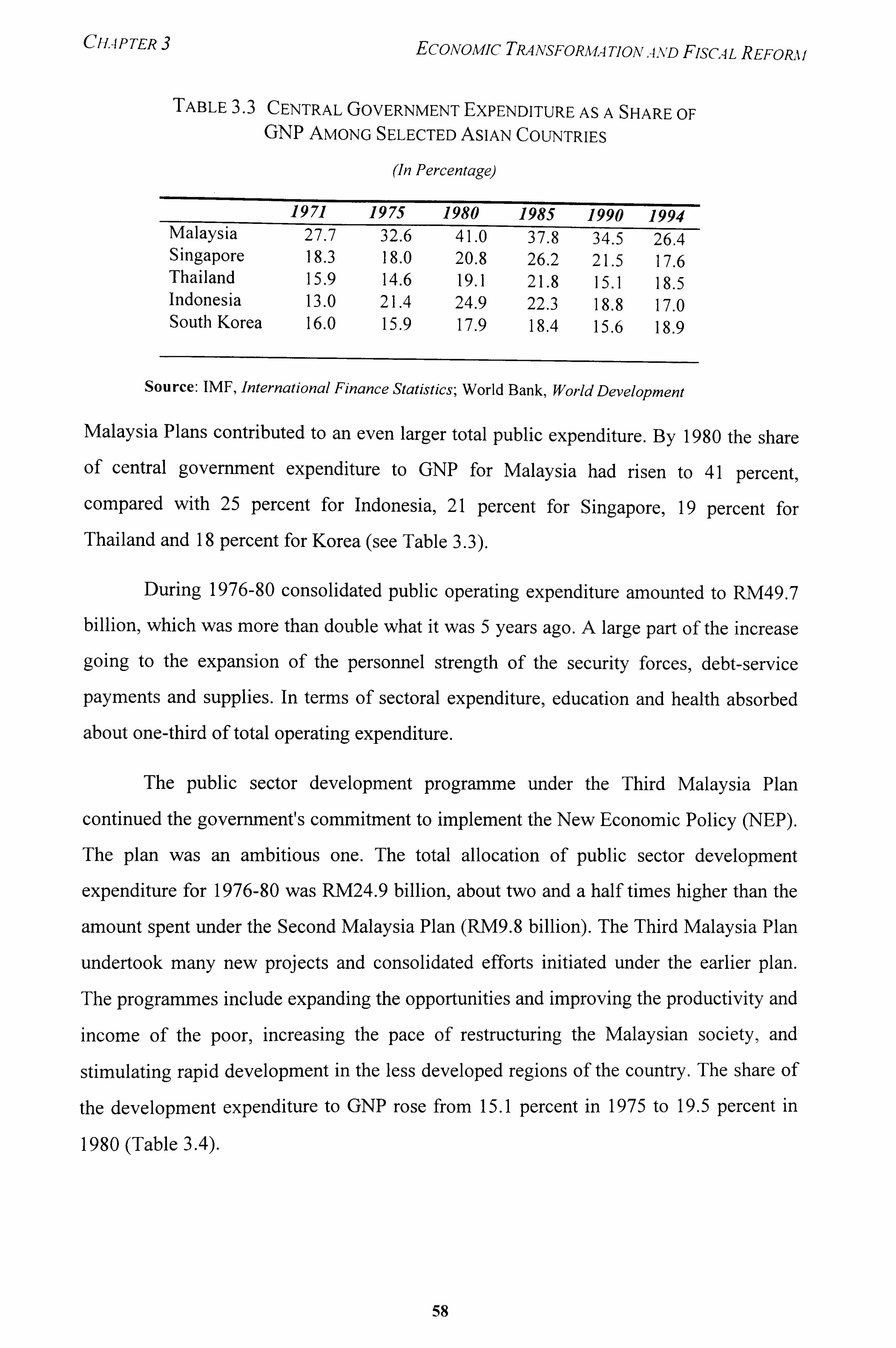
CHAPTER 3 EcoAromic TRANSFORA, 1.4TION, 4., %, D Fisc, 4L REFOPll

TABLE 3.3 CENTRAL GOVERNMENT EXPENDITURE AS A SHARE OF GNP AMONG SELECTED ASIAN COUNTRIES

(In Percentage)

1971 1975 1980 1985 1990 1994 Malaysia 27.7 32.6 41.0 37.8 34.5 26.4 Singapore 18.3 18.0 20.8 26.2 21.5 17.6 Thailand 15.9 14.6 19.1 21.8 15.1 18.5 Indonesia 13.0 21.4 24.9 22.3 18.8 17.0 South Korea 16.0 15.9 17.9 18.4 15.6 18.9

Source: IMF, International Finance Statistics; World Bank, World Development

Malaysia Plans contributed to an even larger total public expenditure. By 1980 the share of central government expenditure to GNP for Malaysia had risen to 41 percent,

compared with 25 percent for Indonesia, 21 percent for Singapore, 19 percent for

Thailand and 18 percent for Korea (see Table 3.3).

During 1976-80 consolidated public operating expenditure amounted to RM49.7

billion, which was more than double what it was 5 years ago. A large part of the increase

going to the expansion of the personnel strength of the security forces, debt-service

payments and supplies. In terms of sectoral expenditure, education and health absorbed

about one-third of total operating expenditure.

The public sector development programme under the Third Malaysia Plan

continued the government's commitment to implement the New Economic Policy (NEP).

The plan was an ambitious one. The total allocation of public sector development

expenditure for 1976-80 was RM24.9 billion, about two and a half times higher than the

amount spent under the Second Malaysia Plan (RM9.8 billion). The Third Malaysia Plan

undertook many new projects and consolidated efforts initiated under the earlier plan.

The programmes include expanding the opportunities and improving the productivity and

income of the poor, increasing the pace of restructuring the Malaysian society, and

stimulating rapid development in the less developed regions of the country. The share of

the development expenditure to GNP rose from 15.1 percent in 1975 to 19.5 percent in

1980 (Table 3.4).

58

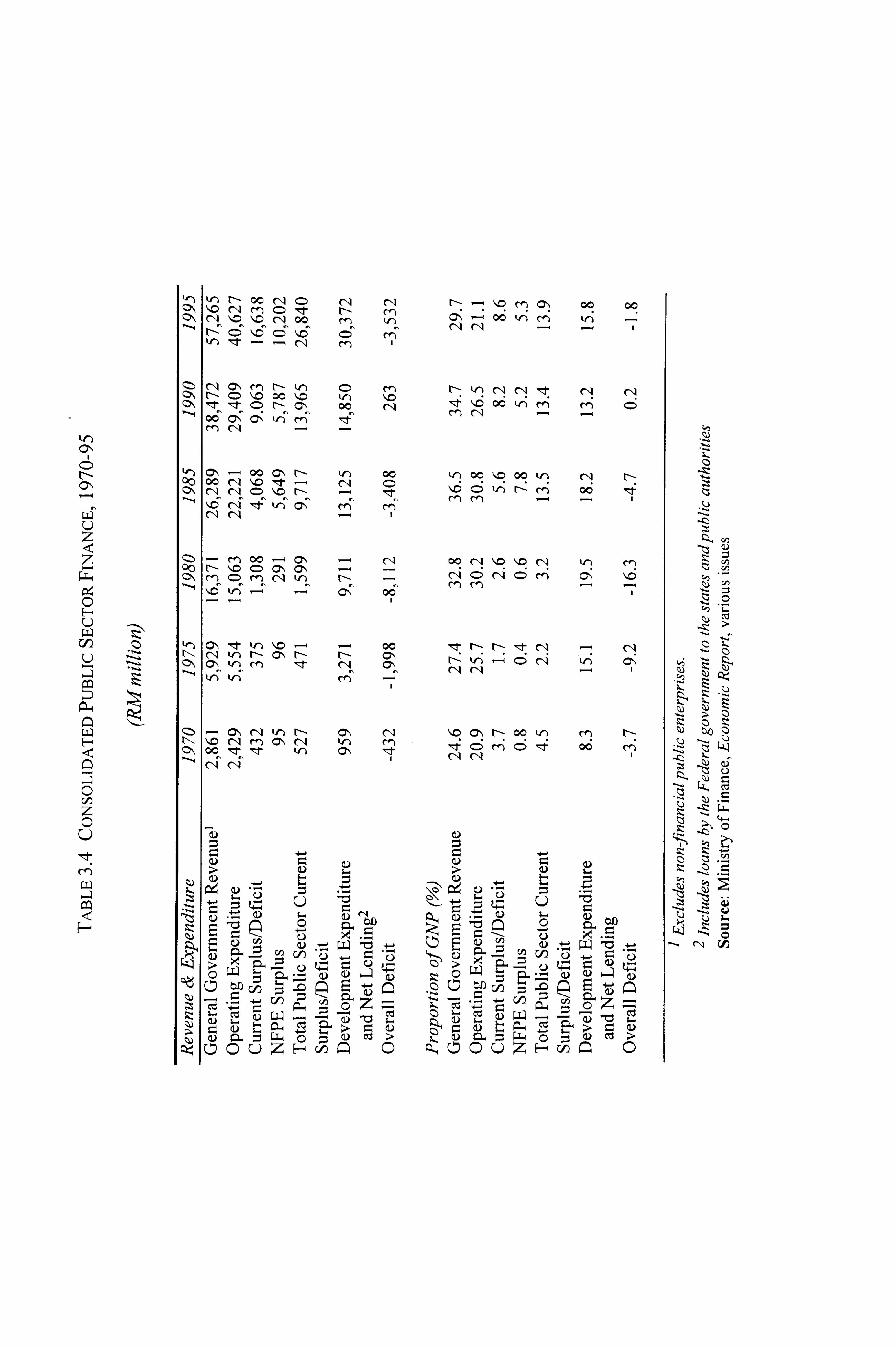
CNI

os\

CD u

1Z1: rf)

-ii\

.

. �-

k-) V-) r- 00 CA CD ri rq r- - 1,0 m cý 00 00 ý> ý'm (-q m CD e r-- cýd ý> rq �0 �0 c-i = rn V')

ýd cý r, ý (1111

ý> r-- C> ýo 00 Ilz v-) 1%c e -e CD r-- vý , c; oý 06 cý, cl ky-ý rlý

cq

"r) (2, - oo c> r- kn 00 V') 00 1,0 00 (n (11 r- 00 ('-l \, O et - CD cq rý CD �0 r- le �0 CD kn r, -, 4 ýd rý, ý, ýý cý,

(Z - rn 00 ---4 Cý --4 CI-1 00 cq "0 ýlo ri V') rn (DO r- 110 CD clý C> ý> rn CD m rý krý r- - (-q C) C-q c> cý cl "0

clý clq V-ý r-- C> CA rq m 0., ci V'ý rn c3

(V r_ C) Q) r_ C) >

4-J

C) rq C)

(D . -tý W -0 . -4-1 C) . 't: ý W "0 . 4-ý

v5 CZ Z cn 1) x- c) ý+. r- Z), C) Gn f, ) A-, r. Z') >Zx C LZ

Ct ýD t)ü cn = -c cEZ ýf) Z 25 tü cn Z -0 cz EZ ýz rý) -= -4- VD = -- CD. Z-. - '-, cn ZJ -V-2 12. Z C) k. - -e (D -0 ;Z cli Lz. > ru (V Z. t- C) =ut. ' Z. m>

CD. ý4 cd > rm. Z :Zu CD r4 (D CD uZ ý- UD Z CD cý, 21 1) cD (-) Zý- CA Z CD

rn

;Z

CH. -IP TER EcONOI fic TRA ASFORAIA Tiav . 4,, \, D Fisc4 L REFORM

In 1971 the ratio of total expenditure of the consolidated public finance 5 to GNP

was 29.2 percent (Table 3.4). It rose to 40.8 percent in 1975 and 49.7 percent in 1980,

with the largest expenditure going to education, defence, infrastructure, agriculture and rural development. In mid-1970s education received close to one-fifth of total public expenditure, while infrastructure accounted for over 12 percent and agriculture and rural development 9 percent. Programmes to improve the physical and social infrastructure

were considered important in improving the life of the people, besides creating a

conducive environment for economic growth and employment generation. Although

there was a current operating surplus during the seventies, the large development

expenditure for the Second Malaysia Plan and Third Malaysia Plan programmes resulted in an overall deficit of RM7.6 billion in 1971-75 and RM12.3 billion in 1976-80.

3.2 Public Expenditure, 1981-95

In the early 1980s, public expenditure on economic services, such as agriculture

and rural development, commerce and industry, expanded rapidly. Health and education

programmes received more resources as well. The government embarked on a major

recruitment exercise to fill up existing vacancies under Operasi Isi Penuh. 6 This was in

response to the general perception that shortage of manpower in the public sector was a

major factor accounting for the large shortfalls in the implementation of the Third

Malaysia Plan programmes. The expansion of the civil service and the salary revisions

pushed up general administration expenditure from RM752 million in 1979 to RM2.1

billion in 1982. Given the increasing size of loans taken by the public sector, the interest

payments for debt servicing doubled from RMI. 3 billion in 1979 to RM2.7 billion in

1982. Expenditure on transfer and subsidies by the Federal government increased

substantially too, from RM2.3 billion in 1979 to RM5.2 billion at the end of 1982.

The sum of operating and development expenditure. 6 Translated literally as 'Operation Fill Up'. In fact, about 180,000 new jobs in government services were

initially planned under the Fourth Malaysia Plan (Malaysia, 1981: 228), but this target was substantially t) revised during the recession as part of fiscal prudence and consolidation in the public sector.

60

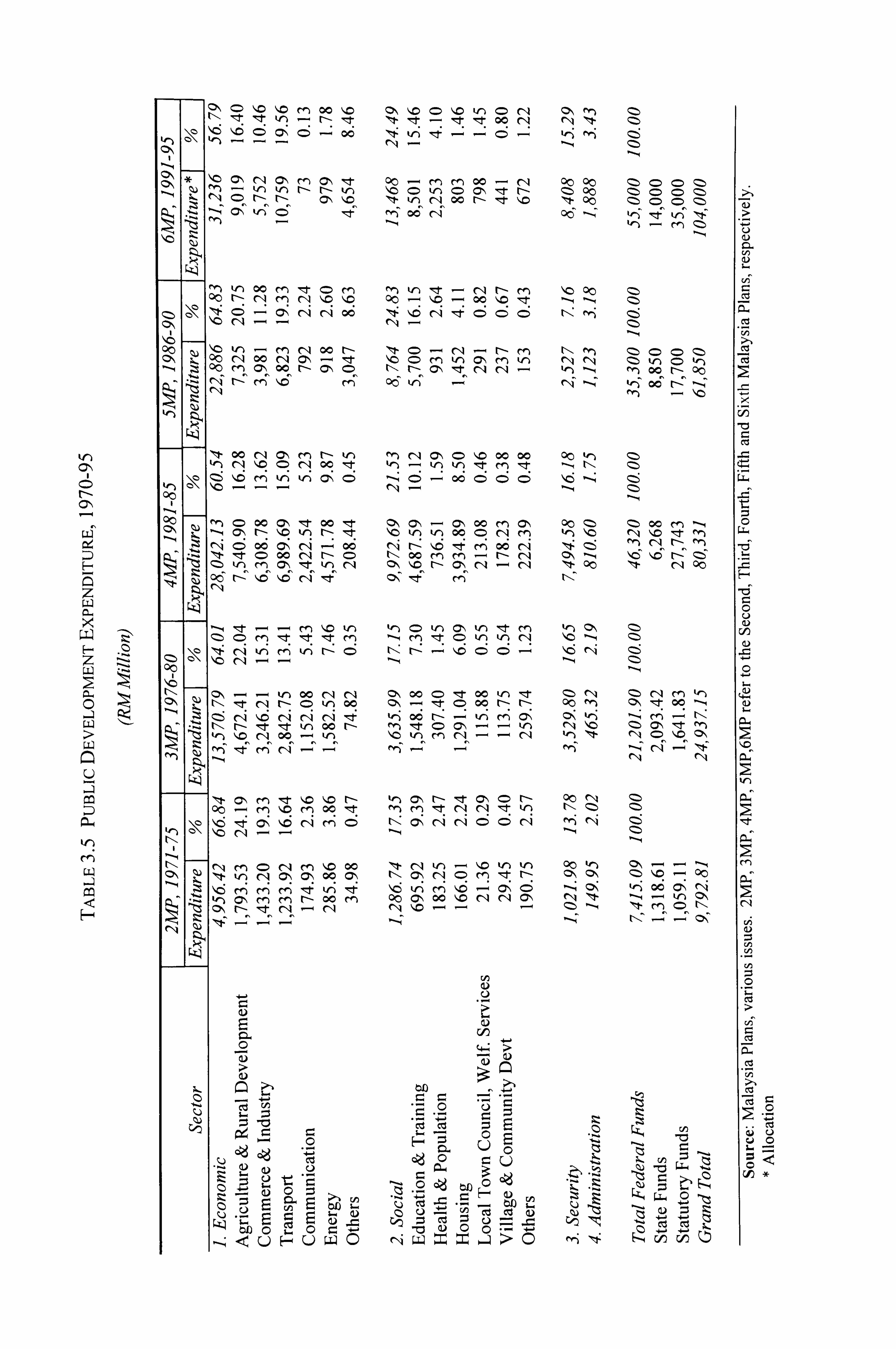
r1)

ý> c> -0 1,0 rn oo �0 t'- ee kl-ý ý r- e

', Z c-, CA o', rn cý -e rn - v) tr) r- r- kr) t"i C> r- t- alý "0 --; cý vý

rn tn 00 m -! T C> m 00 t-- rq m" "C ý, o ,, -1- 6 cq 00 1ý0 rq

"o kf) - m " 00 r-- 00 N 00 C14 Cý - tt oo m (7ý 00 r- (7ý, c)

'Iýt N Cý r-- V") 00

en C) 00 C*N Itt 00 Itt 1 (01-1 r- IC V-) r- Itt

6 C06 Cý C'i -. o6 I: t C) 00 ("1 r- C-) kr) m CIA Itt kn "

06 rz 116 116 CNý llztý' IN

Itt --M

kn m kr; \0 CA --4 -0

kn C14 " r- kn 00

kn 00 r- kn ý, c " 00 - kf)

"tt Cý, en tl- "o I'D t-- 00 - rn 1.0 rn 00 , 1-

110 4 Cý N

N m C) " m 1ý0 00 , \-t C, ý cy" 00 \cs cl; 4 klý tn Cýl m m rl- 00 cn ON r- tT " - Cq

1)

. U U C. )

l' Z Z E - 5 rz u u . - r. ý- u

CD

IC C> \ýc tf) C) 'It - 00

00 C) C) a, llzt r-- V) 00 r- Itt \10

rn V) e- rA r- m 00 - \Z - 00 1,0 mt -In- 110 rq -zý C> CD C) r"ý -

'11- CD - rl - r- rn

en Cý C) 11C 00 00 kn kr) -ýt m Tt

C) 06 C) (6 6

F l C% clý 00 m Cý, o kfý tn 00 c) C-4 C'. )

00 m rn ON O'ý cl CIA

cpý rrý

tn CIN kn c? ) (= kn tn C14

00 C> 00 tr) Iti- CN - -1- 00 1-- t-

kn 06 r-- - Vý al rn zt C) C) - V) \%o m CA

'Iýt rj kn -- \ýc tr) kn clý " C) m IZI- rl-

klý cl; 110 - (71 6 00 a, 00 110 C14 C14 a, N \, c -. 4 ý -4

-- ,Z

. - tü

Q2

-a Q) 0 0 . - Zj rli ý2 Z Z ý CD

CD CD (Z2) Z) 00 (Z CD (= (Z2) '11- CD CD (Z 06 "r (rý Illz kr, ) - rn (Z

m

110 CO

t, -, rn r111 f", 1

(ZS <Z

(Z) V_ý CD (-ý 00 t-

uý rZ, rn - \ýc

00 In , t"

00

00 en Oý klý N 'No

r-I (Z)

Oo kn

rl

z

-. . -

..

(Z oo m ---4 r1-1 ýo rn rn cli rn

Z) (Z zý (Z

4

czý C, 4 m

%C

Z) (Z

cs (Z

(: z "o - 00

00 al N ý-

lý

-a

-4-4 -4--1 ; ý.

E2 En En C. ý

cz

C', cw

03

CHAP TER 3 EcONomic Tpi ., %'SFOR, If, -l TIO, \'. 4,, %, D Fisc. 4 LR EFORA I

During this period the Federal government increased transfers for pensions and to the

state governrnents, as well as subsidies for agriculture, scholarships, textbook loans

programmes, and milk and food programmes. Together, these factors contributed to the

rapid increase in the current expenditure of the government that rose from 26 percent of GNP in 1979 to 31 percent in 1982.

Among the four Malaysia plans during 1970-90, the Fourth Malaysia Plan had

the largest development expenditure. In terms of Federal Government expenditure, it was

more than twice the size of the Third Malaysia Plan and about one-third larger than the

Fifth Malaysia Plan (Table 3.5). The scale of fiscal expansion in 1981 and 1982 was

unprecedented as the government increased the development budget, as shown in Figure

3.19. Government development expenditure alone for 1981 and 1982 was over 23

percent of GNP, compared to the average of 14.3 percent in 1976-80. The largest

category of development expenditure was for defence and internal security. A large part

of the expenditure went to infrastructure, in which the allocation for transport, education

and irrigation doubled between 1980 and 1982.

Commerce and industry was the other area which received increased allocation of

funds in the Fourth Malaysia Plan. Although part of the expenditure was financed from

profits generated by the National Petroleum Corporation (PETRONAS) and its

subsidiaries, the consolidated public sector deficit increased from 8 percent of GNP in

1979 to 22 percent and 19 percent in 1981 and 1982, respectively (World Bank, 1989: 6).

When financial resources turned out to be lower than expectations, it became clear that

this expenditure pattern was not sustainable. Expenditure cutbacks and rescheduling of

projects were initiated with the launching of the Mid-Term Review of the Fourth

Malaysia Plan. The task of reducing the original allocations in midstream could not have

been an easy one since most of the projects were in different stages of implementation,

with contractual obligations for the government. The larger projects that were started in

one plan period would continue into another and require public resources for their

successful completion and operation. In addition, the programmes for the eradication of

poverty and restructuring of society were not to be affected by the cutbacks. The

consolidation of public sector expenditure that ensued set the stage for the approach that

was to be applied throughout the decade and into the nineties. This is illustrated by the

62

CHAPTER EcONOA, fIc TRANSFORMA TION. -iND FISCAL REFORAI

fact that the public sector development allocation in the Fifth Malaysia Plan was RM 10 billion smaller than the Fourth Malaysia Plan allocation.

Recession years: The operating expenditure during the recession years was kept

within one-quarter the size of GNP. The debt service charges for 1985-86 had risen quite dramatically. About one-fourth of the total operating expenditure of the Federal

government (or over RM5 billion) were allocated to pay interest on outstanding loans

and make contributions to the sinking fund. By comparison, the amount allocated for this

purpose in 1980 was only 11 percent of total operating expenditure. The rapid

appreciation of the Yen by 34.7 percent during 1985-86 increased Malaysia's debt service

obligations substantially since loans from Japan constituted 20 percent of Federal

government outstanding foreign debt in 1985. The other major expenditure was for social

services so that the quality of essential social infrastructure, such as education and health,

was maintained even during the recession. About two-thirds of the expenditure for social

services went to education and another one-fifth to health services.

In the development expenditure of the Federal government, spending for security

registered negative growth of around 38 percent for both 1985 and 1986. Allocation for

social services increased by 12 percent in 1986 as a result of increased spending for

education and housing. For the economic services, the expenditure for agriculture and

rural development, public utilities and commerce and industry in 1986 fell below the

1985 level. This was partly due to planning and implementation problems arising from

the reordering of programme priorities as well as from contractors who were unable to

complete projects on time. However, the expenditure for transport and communications

increased by 32 percent to provide for greater private sector expansion.

The consolidated public sector deficit fell to 7.2 percent of nominal GDP in 1985,

but rose again to 13.1 percent a year later. It is generally difficult to cut budget deficits

during recession when revenues are low. Revenue derived from direct taxes declined by

6 percent in 1985-86 as the income of companies, individuals and petroleum operations

fell as a result of the recession. In 1986 very little revenue was collected from the export

of rubber and palm oil which were facing depressed prices.

63

CHAP TER 3 EcoNavic TPANSFORAL4TJOA'. 4, vD FISC. 4L REFORM

The narrowing public sector deficit in 1985 was attributed to the increased profits from the NFPEs, especially from the petroleum and gas operations. When the price of

crude petroleum fell by 47 percent from US$27.60 per barrel in 1985 to US$14.80 per barrel in 1986, this drastically cut into PETRONAS' profits and reduced expected Federal

goverm, nent revenue since petroleum and gas contributed 22 percent of the total revenue. The NFPE accounts went into deficit again, thereby exacerbating the fiscal deficit.

To stimulate growth without fiscal expansion, the Anti-Recession Committee was

formed to draw up short-term programmes to generate growth in employment and output.

Growth in money supply (Ml) increased from 2.8 percent in 1986 to 13.0 percent in

1987, while nominal interest rate declined. The average rate of discount for three month

treasury bills declined from 4.12 percent (1985) to 3.22 percent (1987) and the base

lending rates from 10.75 percent (1985) to 7.50 percent (1987). The New Investment

Fund (NIF) and a small industries development fund was established to increase the

credit supply in the economy.

Expenditure, 1986-95. Operating expenditure during this period was kept within

manageable limits and grew at 6.3 percent per year. This comparatively slower growth

was in keeping with the fiscal discipline following the 1985-86 recession. The

expenditure on emoluments, which accounted for 36 percent of total current expenditure,

increased by 5.8 percent per annum due to annual salary increments and salary

adjustments for civil servants. In line with financial prudence, spending on supplies and

services as well as transfers to government agencies were curtailed selectively.

With economic recovery, public sector development programmes that facilitate

growth were reinstated and the total development expenditure for the Fifth Malaysia

Plan, 1986-90, was RM35.3 billion. Programmes on agriculture and rural development

were aimed at poverty eradication and restructuring of society. Public investment grew

by 15 percent per annum during 1988-90, particularly for upgrading and expanding the

infrastructure facilities to ease constraints and bottlenecks to growth and cope with the

demands of the expanding trade and industry. The government placed emphasis on social

and physical infrastructural development to improve the quality of life as well as to

provide the country with a broad-based foundation to facilitate investments and growth.

64

CILAP TER ECONOMIC TRANSFORA IA TIONAND FISCA L REFOkk f

Improvements in the financial position of the public sector enabled additional

resources to be allocated for the Sixth Malaysia Plan, 1991-95. Although its total public

sector development allocation (RM104 billion) was much higher than that for the Fifth

Malaysia Plan (RM61.8 billion), the ratio of development expenditure to GNP was

maintained at 14 percent. This reflects the government's on-going efforts at fiscal

prudence and more efficient management of public sector programmes and finances,

following the directions established since 1983. The bulk of the increase in expenditure

was directed towards facilitating economic growth and the provision of infrastructure to facilitate expansion of the private sector. In addition, the'social sector was given one

quarter of the Federal government development allocations to improve services in

education and training, health, and housing. The poverty eradication programmes were

directed towards the hard-core poverty groups, while the programmes for restructuring

society were devoted to education and training, as well as the development of

Bumiputera commercial enterprises.

3.3 Public Revenue and Finance, 19 70-80

As the range and complexity of government operations increased during the

1970s,, the country adopted prudent fiscal and monetary policies to have low price

inflation and high credit worthiness. The general government revenue rose from RM2.9

billion in 1970 to RM16.4 billion in 1980. The average growth rate of total revenue was

15.7 percent per year during the first half of the decade and accelerated to 22.5 percent

per year in the second half of the decade. For the five-year periods corresponding to the

Malaysian development plans, the total government revenue for 1971-75 was RM22.0

billion and it increased to RM54.7 billion in 1976-80 (Malaysia, 1981: Table 6-6). As a

share of GNP, this corresponds to 34.1 percent for 1971-75 and 58.6 percent for 1976-80.

The rapid growth of public revenue in the late seventies was fuelled by

exceptional set of favourable conditions. Rubber and tin prices reached their peak for the

decade with their 1980 prices more than triple the 1970 prices (see Figure 3.5). The rapid

growth in export volume for oil palm arising from the expansion in oil palm cultivation

in the 1960s and early 1970s as well as the increased production capacity of petroleum

from new oil fields off shore coincided with the buoyant commodity prices. The good

65

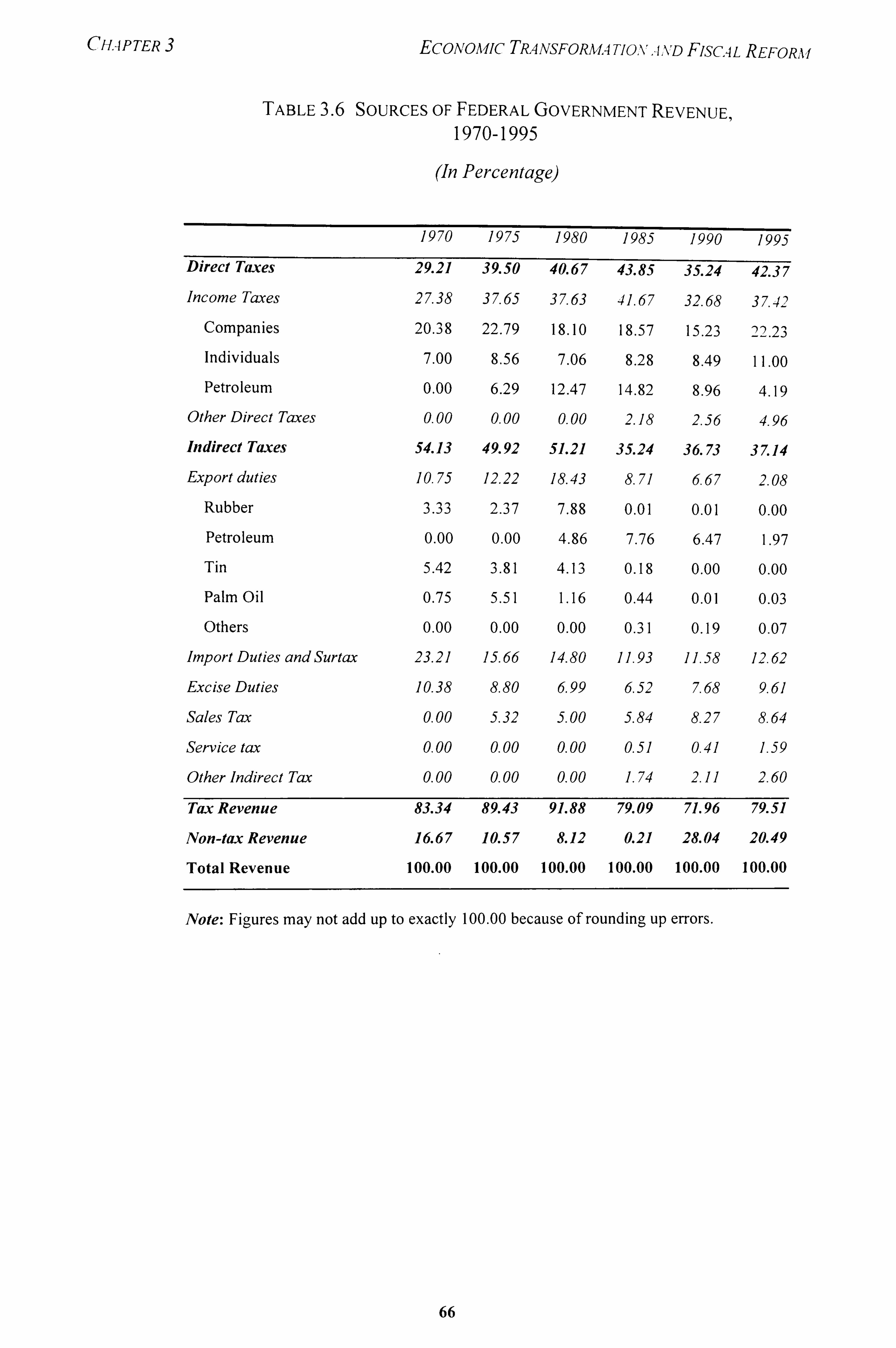
CHAPTER EcONOAlIc TP, 4NSFORA4,4 Tlo, \'. -i, \D Fisc. AL REFORM

TABLE 3.6 SOURCES OF FEDERAL GOVERNMENT REVENUE, 1970-1995

(In Percentage)

1970 1975 1980 1985 1990 1995

Direct Taxes 29.21 39.50 40.67 43.85 35.24 42.37

Income Taxes 27.38 37.65 37.63 41.67 32.68 37.42

Companies 20.3'8 22.79 18.10 18.57 15.23 2 2.2 3

Individuals 7.00 8.56 7.06 8.28 8.49 11.00

Petroleum 0.00 6.29 12.47 14.82 8.96 4.19

Other Direct Taxes 0.00 0.00 0.00 2.18 2.56 4.96

Indirect Taxes 54.13 49.92 51.21 35.24 36.73 37.14

Export duties 10.75 12.22 18.43 8.71 6.67 2.08

Rubber 3.33 2.37 7.88 0.01 0.01 0.00

Petroleum 0.00 0.00 4.86 7.76 6.47 1.97

Tin 5.42 3.81 4.13 0.18 0.00 0.00

Palm Oil 0.75 5.51 1.16 0.44 0.01 0.03

Others 0.00 0.00 0.00 0.31 0.19 0.07

Import Duties and Surtax 23.21 15.66 14.80 11.93 11.58 12.62

Excise Duties 10.38 8.80 6.99 6.52 7.68 9.61

Sales Tax 0.00 5.32 5.00 5.84 8.27 8.64

Service tax 0.00 0.00 0.00 0.51 0.41 1.59

Other Indirect Tax 0.00 0.00 0.00 1.74 2.11 2.60

Tax Revenue 83.34 89.43 91.88 79.09 71.96 79.51

Non-tax Revenue 16.67 10.57 8.12 0.21 28.04 20.49

Total Revenue 100.00 100.00 100.00 100.00 100.00 100.00

Note: Figures may not add up to exactly 100.00 because of rounding up errors. Z-: ) t: )

66

CHAP TER EcONOAfIc TRANSFORAIA TION AND FISCAL REFORAI

export performance for the commodities coupled with the booming business conditions contributed to a marked increase in revenue from direct and indirect taxes in the country.

Direct taxes, which contributed 29.2 percent of the total Federal government

revenue in 1970,, increased to 40.7 percent in 1980 (Table 3.6). Following the growth of income and improvement in the tax collection machinery, revenue from this source was

growing at 23.2 percent per year during the seventies. Income tax on petroleum

production began to increase in importance in the second half of the decade. Taxes on foreign trade and domestic indirect taxes grew at an average rate of 18.5 percent per year

as a result of increased volume of foreign trade, increased prices of both export and import commodities, as well as accelerated growth of domestic production. To expand

the tax base, sales tax was introduced in 1972 and service tax in 1975. The sales tax is an

ad valorem single stage tax imposed at the import and the manufacturing levels.

Exemptions were given to smaller manufacturers, certain food stuffs, building materials

and books, as well as to exports. The service tax was imposed on large hotels and

restaurants.

In view of the large development expenditure of the Second and Third Malaysia

Plans, the overall deficit grew from RM7.6 billion in 1971-75 to RM12.3 billion in 1976-

80. The larger deficit in the Third Malaysia Plan called for higher level of borrowing

without creating inflationary pressure on the economy. Domestic borrowing provided

between half to two-thirds of the fund requirements during the decade (see Table 3-7).

The bulk of this source was derived from the non-bank private sector, such as the

national social security organisation, National Savings Bank and insurance companies.

As a result of higher revenue base, the amount of domestic borrowing during 1976-80

was much lower than the amount targeted in the Third Malaysia Plan, that is, RM7.8

billion of actual borrowing as against the target of RM1 I billion. At this level of resource

mobilisation, the monetary expansion was consistent with the growth in nominal GNP.

The public sector programmes under the Third Malaysia Plan was undertaken within an

environment of financial and price stability as is evident from the consumer price index

67

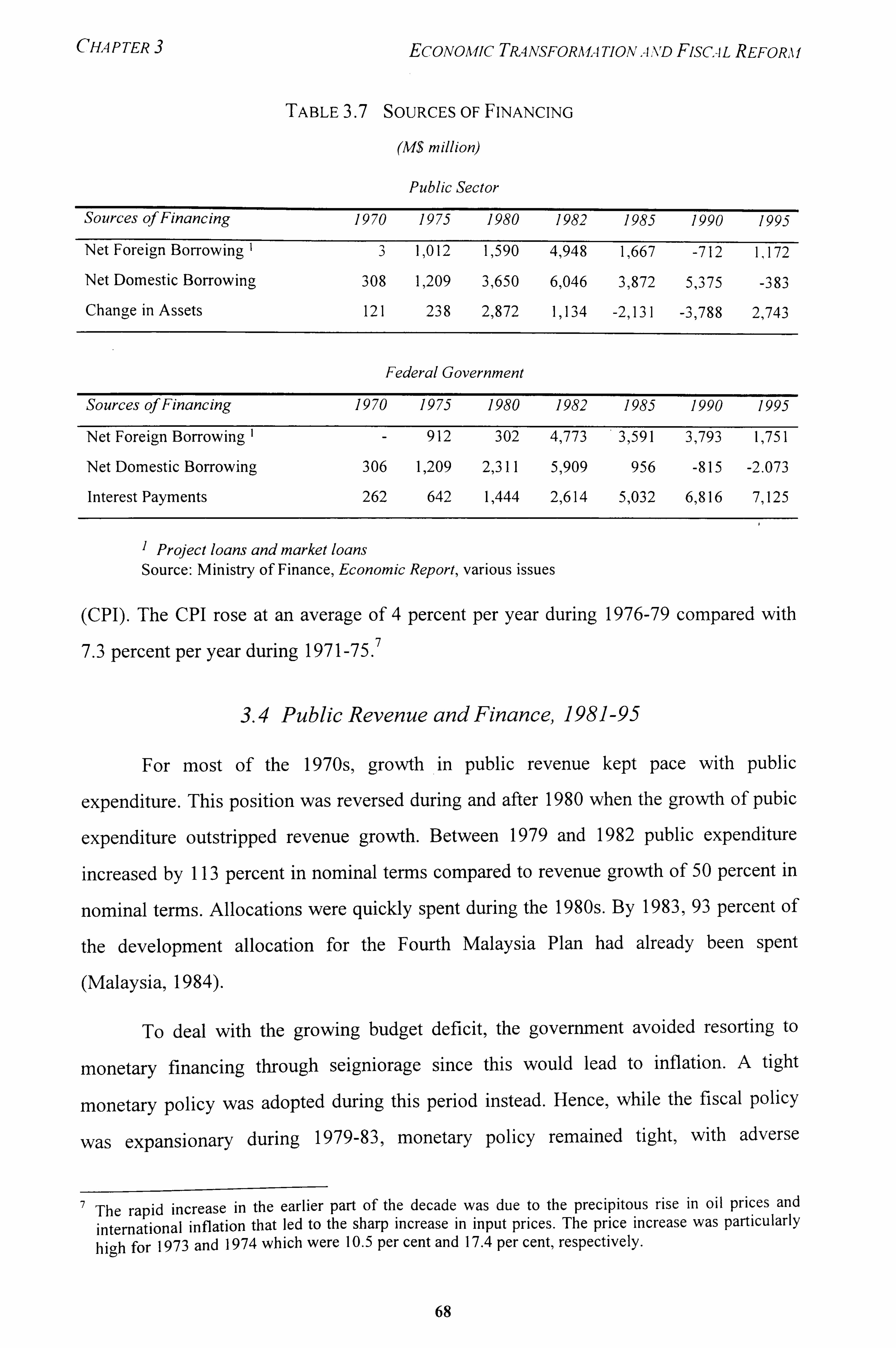
CHAPTER 3 EcONOAlIc TPANSFORAI, 4TlON. -i, vD FJsc, -IL REFORM

TABLE 3.7 SOURCES OF FINANCING

(M$ million)

Public Sector

Sources of Financing 1970 1975 1980 1982 1985 1990 1995

Net Foreign Borrowing 1,012 1,590 4,948 1,667 -712 1,172

Net Domestic Borrowing 308 1,209 3,650 6,046 3,872 5,3 75 -33 83

Change in Assets 121 2-33 8 2,872 1,134 -2,131 -3 ), 788 2,743

Federal Government

Sources o Financing )f 1970 1975 1980 1982 1985 1990 1995

Net Foreign Borrowing I - 912 302 4,773 3,591 3,793 1,751

Net Domestic Borrowinc, 306 1,209 2,311 5,909 956 -815 -2.073 Interest Payments 262 642 1,444 2,614 5,032 6,816 7,125

I Project loans and market loans Source: Ministry of Finance, Economic Report, various issues

(CPI). The CPI rose at an average of 4 percent per year during 1976-79 compared with 7

7.3 percent per year during 1971-75 .

3.4 Public Revenue and Finance, 1981-95

For most of the 1970s, growth in public revenue kept pace with public

expenditure. This position was reversed during and after 1980 when the growth of pubic

expenditure outstripped revenue growth. Between 1979 and 1982 public expenditure

increased by 113 percent in nominal terms compared to revenue growth of 50 percent in

nominal terms. Allocations were quickly spent during the 1980s. By 1983,93 percent of

the development allocation for the Fourth Malaysia Plan had already been spent

(Malaysia, 1984).

To deal with the growing budget deficit, the government avoided resorting to

monetary financing through seigniorage since this would lead to inflation. A tight

monetary policy was adopted during this period instead. Hence, while the fiscal policy

was expansionary during 1979-83, monetary policy remained tight, with adverse

7 The rapid increase in the earlier part of the decade was due to the precipitous rise in oil prices and international inflation that led to the sharp increase in input prices. The price increase was particularly high for 1973 and 1974 which were 10.5 per cent and 17.4 per cent, respectively.

68

CHAP TER ECONOxfic TPNNSFORMA Tlo, %', -i vD FiSCA L REFORA f

implications for interest rates and depressed private investment. Monetary growth in the first half of the 1980s decelerated not only because of the decline in the net foreign

reserves but also due to the fall in net lending to the public and private sectors. In fact,

the growth rate of MI (which consists of currency and demand deposits of the private

sector) declined in 1983 and 1984, even before the contraction of economic activity in

1985 (Ariff, 1991: 33). The annual rate of growth of money supply and private sector liquidity declined every year during 1980-84, while inflation was relatively low at an

average rate of 4.7 percent.

The deficit was financed from both domestic and foreign borrowings. Domestic

borrowing by the Federal Government rose in the early eighties and peaked in 1982 at

two and the half times the level of the domestic loans made in 1980. The more important

source of financing the deficit was borrowing from external sources, rose from RM302

billion in 1980 to RM4.8 billion in 1982. As a result of the large financial resource

requirement in the early 1980s, borrowing from foreign sources increased sharply and

closely matched the amount borrowed from domestic sources (Figure 3.20). As a result

the Federal government outstanding foreign debt as a ratio of GNP rose from 9 percent in

1980 to an unprecedented level of 32 percent in 1985.

During 1980-85, the tax revenue was around 23-25 percent of GNP and registered

a growth rate of 5.5 percent per annum. This was a considerable achievement since this

period also coincided with tax cuts as well as the fall in export tax receipts. With the

decline of commodity prices, the collection from export duties for 1985 was RMI. 8

billion or 30 percent lower than the RM2.6 billion collected in 1980. This decline was

more than compensated by the revenue from direct and indirect taxes on petroleum

which doubled from RM2.4 billion in 1980 to RM4.8 billion in 1985. In 1981 for the

first time PETRONAS remitted dividends on its earnings to the goverm-nent and emerged

as a major financier of government deficits through purchases of the government debt

(World Bank, 1983: 49).

Budget deficit. The consolidated public sector budget deficit 8 to GDP increased

markedly from 7.5 percent in 1979 to a peak of 19.7 percent in 1981. Deficits of this

8 The consolidated public sector account refers to the combined revenue and expenditure of the Federal

government, state government and non-financial public enterprises.

69

CHAPTER 3 EcONOA fic TP, 4 NSFORMA Tio. \,,, i,, \, D Fisc. 4 L REFORA f

magnitude were unparalleled given that the level reached in the previous decade was no higher than II percent of GDP. The widening deficit of the public sector was not only attributed to the counter-cyclical policies, but also the reduction in tax revenue as a result of poor commodity prices and expenditure growth of the expanding public sector.

In 1983, the government adopted measures to consolidate and rationalise the

public sector to control the large public sector deficit. The Federal government development expenditure fell from RMII. 5 billion in 1982 to RM8.4 billion in 1984,

representing a reduction of 14.4 percent per annum. Uncommitted projects were

suspended, while projects in their initial stages that did not have high social or economic

costs were terminated or rescheduled. The government instituted a wage freeze in the

public sector and adopted cost saving measures at all levels of government. These

measures brought immediate results since the expenditure on wages and salaries as well

as purchases of goods and services came to a standstill in 1983. Transfers and subsidies, the second largest category of expenditures, grew by less than 3 percent in nominal

terms, compared with an average of 36 percent two years before. As a result of increasing

debt commitments, the interest payment was the only item showing a rapid increase of 40

percent over the 1982 position. The effectiveness of the fiscal rationalisation on the

government budgetary position were reinforced by a healthy operating surplus arising from PETRONAS petroleum operations and the sharp reduction in the development

budget. Despite the fiscal austerity adopted by the Federal government, the non-financial

public enterprises were not affected by these measures. They continued to increase their

own investment programmes from domestic and foreign sources of funding. This

situation was brought under control in 1984 when they were made accountable to the

Treasury with regards to their investment and financing programmes.

Revenue, 1986-95. The general government revenue grew by 8 percent per annum

during 1986-90, but as a percentage of GNP it declined from 36.5 percent in 1985 to 29.7

percent in 1995. The decline had been attributed to the deterioration of the overall tax

buoyancy which fell from 1 .0 during the Fourth Plan period to 0.6 during the Fifth Plan

period (Malaysia, 1991b: 67). During the 1980s, there was increased tax exemptions,

allowances and incentives given to the private sector to promote investment as well as

lower petroleum and commodity prices.

70

CHAPTER EcONomic TRANSFORAIA TION, A., ND FisCAL REFORAf

During 1987-95, the period of recovery and rapid economic growth, company income tax and individual income tax grew at 18.2 percent per annum and 14.2 percent,

respectively, as profits and personal income increased during the economic upswing. Income tax derived from petroleum companies increased to RM2.6 billion in 1990 but

declined thereafter as production and oil price declined in the early nineties. Indirect

taxes also recorded a rapid growth of 21.7 percent per annum and accounted for 37

percent of total federal government revenue by 1995. The main sources of revenue were from import duties, surtax, excise duties and sales tax which arose from higher imports,

stronger consumer spending, and improvements in the tax administration.

The overall deficit narrowed,, brought about by prudent public sector spending, increased revenue accruing from rapid economic recovery, as well as the operating

surplus of NFPEs. The overall deficit in the consolidated public sector finance from 4.9

percent of GNP in 1987 to around zero in 1989-90, before rising to 1.8 percent of GNP in

1995. Public sector borrowing to finance the deficit declined rather spectacularly from

RM7.0 billion in 1987 to RM789 million in 1995. With the exception of 1995, the source

of financing for 1987-94 came from non-inflationary domestic sources.

4. POLICIES FOR THE NINETIES AND BEYOND

4.1 Vision 2020 and National Development Plan

The year 1990 marked the end of the First Outline Perspective Plan (OPP I). During the

20 years of its implementation, Malaysia had come a long way in socio-economic

development. Its economy grew at an average rate of 6.7 percent per annum, while its per

capita income doubled. Exports of goods and services grew by 9.2 percent per annum

accompanied by the expansion of manufactured exports that contributed 60 percent of

total exports in 1990.

Much progress had been achieved in addressing the problems of poverty and

socio-economic inequality among ethnic groups. Poverty among all ethnic groups was

significantly reduced. The proportion of poor households in Peninsular Malaysia

declined from 49.3 percent in 1970 to around 15 percent in 1990 (Malaysia, 1991 a: 9).

71

CHAP TER 3 EcONO, kfIc TK4ASFORA IA Tjo, \'ýA ý\D FISC, 4 LR EFORA f

During the same period, the proportion of Bumiputera employed in the manufacturing

sector increased from 28.9 percent to 49.1 percent, while their employment in agriculture fell from 50.3 percent to 22.2 percent. More Bumiputera were also engaged in

professional, managerial and technical occupations, while their share ownership9 grew from RM125.6 million in 1970 to RM22,298 million in 1990, accounting for 20.3)

percent of total share ownership. Although Bumiputera share ownership fell short of the NEP target of 30 percent, the growth had been remarkable. Bumiputera share ownership

registered an average annual growth of 30 percent (as against 16 percent for overall

growth) during the OPP1 period and was 177 times larger in 1990 than it was twenty

years ago.

After the end of the OPPI period, the direction for the country's development

efforts for the next thirty years will be guided by the policy pronouncement of Vision 10 2020 . Under this vision, Malaysia strives to be a united, fully developed nation by the

year 2020. The development approach spans several dimensions, encompassing not only

economic growth, but also other aspects of development, such as the achievement of

national pride and confidence, political maturity, spiritual values, liberal and tolerant

society, scientific and technological progress, as well as a caring, economically just,

competitive and prosperous society.

The first decade within this thirty years development perspective is addressed by

the Second Outline Perspective Plan (OPP2) which sets out policies, strategies and

targets for 1991-2000. As in the First Outline Perspective Plan, national unity will

remain the over-riding goal of socio-economic development. The basic strategies of NEP

are given a new focus: (a) eradicating hard-core poverty; (b) developing an active

Bumiputera Commercial and Industrial Community; (c) greater involvement of the

private sector in restructuring society; and (d) greater emphasis on human resource

development. Poverty eradication programmes will target on the hard-core poor and the

poverty rate is projected to decline from 17.1 percent in 1990 to 7.2 percent by the year

2000. The restructuring strategy will focus on developing a Bumiputera Commercial and

9 This include the share holdings of Bumiputera individuals and trust agencies.

10 In the inaugural meeting of the Malaysian Business Council in February 28,1991, the Prime Minister

presented a paper entitled, "Malaysia: The Way Forward", which charted out the vision of Malaysia as a fully developed nation by the year 2020.

72

CHAP TER EcONomic Tk4 AISFORAIIA TION A ND FISCA L REFORA f

Industrial Community to increase the participation of this community in the corporate and non-corporate sectors. The growth target for the next 30 years will require the doubling of GDP every 10 years or achieving a sustained average growth of 7 percent per annum throughout the period. By the year 2000 the share of manufacturing in GDP is

projected to increase to 37 percent and manufacturing exports will account for 81 percent

of total exports.

4.2 Frameworkfor Future Policies

The government aims at maintaining economic stability and growth by formulating policies that improve efficiency, productivity and macro policy management. It will seek an appropriate balance of fiscal, monetary and trade policies, help revitalise

the primary sector, improve physical and social infrastructure, and enhance the business

environment. In particular, the Second Outline Perspective Plan enumerates four policy

areas that will be given attention (Malaysia, 1991 a: 8 8-93):

(1) Improvement of economic efficiency. Policies will be formulated to increase

the competitiveness of the industrial sector and promote greater neutrality in

the use of labour and capital. Tariff protection will be reduced or removed and

the tax and incentive systems will be reformed. The privatisation programme

will continue, while public-private sector co-operation and R&D efforts will

be intensified. The tax and incentive systems will be reformed such that they

will promote reinvestment, strengthen government revenue as well as achieve

the distributional objectives in a more efficient manner.

(2) Policies to support private investment. Wage increases should correspond to

productivity growth. The regulated prices of industrial raw materials will be

reduced to lower the cost of production. The public sector will play a

supportive role by improving the physical and social infrastructure as well as

the administrative procedures to strengthen business confidence. The financial

and capital markets will be strengthened to mobilise funds for private

investments.

73

CH, 4pTER Eco, %,, o, i, fic TRAN'sFopui. 4 TioA,. 4, \, D Fisc. -I L REFOR. ý f

(3) Human resource development. Priority will be given to develop a large pool

of skilled manpower for modern services and industry. Training programmes

will be market oriented and the education and training systems will be

monitored more closely so that there is better matching of the demand and

supply of skills in the labour market.

(4) Policies to stabilise public debt, deficits and spending. Consistent with its

policy to develop a private sector-led export-oriented economy, the

government will refrain from an expansionary fiscal stance and involvement

in commercial activities. To consolidate public sector finances, the

government will reduce subsidies, strengthen the revenue base, and increase

the effectiveness of tax administration. It will also encourage greater use of

user-charges and self-financing in the funding of specific programmes. There

will also be less reliance on external market borrowing to reduce the country's

exposure to exchange rate fluctuations.

4.3 Implications for Fiscal Policy

There are several fiscal policy implications from the four policy areas of the

Second Outline Perspective Plan. First, the objectives and targets of the National

Development Policy are to be pursued in the environment of sustained economic growth,

where the leading growth sectors will be manufacturing and services-related activities.

Accordingly it is reasonable to expect that the government will adopt fiscal policies that

would help the manufacturing sector to be efficient, competitive and broad-based. Some

of the measures would include reviewing the fiscal and tariff-related policies and

removing factor price distortions. In view of the focus of the National Development

Policy towards eradicating poverty, the government would be concerned that changes in

the fiscal policy should have minimal negative impact on poor households. In addition,

taxes that affect the income of poor households are also candidates for review, such as

taxation on agriculture. In this regard, most export taxes on primary commodities, such

as rubber, tin, and palm oil, have already been reduced or completely removed because of

their regressive effect on poor households. There would also be continuing investment to

raise the quality of human resource through improvements in health and education. It is

74

CHAP TER EcoA, Omlc TR-iA'SFORA IA TIOA, '. 4,, \TD Fisc. 4L REFORA f

possible that further tax incentives would be offered to institutions and employers that contribute to increasing the quality of human resources in the country.

Second, -the maintenance of macroeconomic stability is crucial to safeguard the

excellent growth record of the country, especially that achieved during the last few years. Any adverse fiscal developments would have to be closely monitored such that public spending would be matched with the revenue base. The restraint on public spending would continue, while public expenditure would be in the areas with the highest payoffs,

such as enhancing the country's economic growth potential and productivity, stimulating

private sector investment, improving the quality of life of the people, and upgrading human capital. In addition, to keep public expenditure on social services small, there

would probably be a more pervasive adoption of user-charges on public services and

amenities. On the revenue side, some taxes would have to be reduced. This is to ensure that that these taxes are not too out of line with the tax regimes of neighbouring countries

or in fulfilment of Malaysia's obligations with regards to international agreements on free trade. To compensate for the revenue loss, the government would probably be

looking for tax handles that can increase revenue with minimal distortions on the

economy. This would imply the move to broaden the tax base and increase the tax buoyancy so that tax revenue would keep pace with or grow faster than the rate of

economic growth. It could also involve tapping into potential sources of revenue and

eliminating unnecessary business tax incentives and subsidies.

Third, the public sector would focus on providing public goods characterised by

market failure such as primary education and preventive health, while reducing activities

that compete with the private sector. On the other hand, there has been increasing private

sector participation in the provision of infrastructure, which in the past was considered

the preserve of the public sector. The provision of social services, health and education

have traditionally accounted for the largest single category in the budget. The

privatisation of non-financial public enterprises during the Fifth Malaysia Plan was found

to be effective in raising the efficiency of providing of infrastructure, reducing the burden

on public finance, and expanding equity ownership for the Bumiputera. With greater

involvement of the private sector in providing physical infrastructure, health and

educational services, the focus for the government in the future would move from direct

75

CHAPTER 3 Ecavo, vfIc TRA ASFORA f -1 TIO, \', 4, ND FisCA L REFORA I

provision of services to the monitoring of standards and regulating the delivery of social services by the private sector.

Fourth, an important consideration for the government is to reform the tax system

so that it could meet expenditure requirements without distorting incentives to work and invest. The wide range of fiscal incentives that are currently offered to the corporate

sector are associated with revenue loss and social and economic costs of inefficient

industrialisation. When the effective rates of protection vary across industries and

categories of operations, the allocation of investment across sectors tend to be distorted,

since business decisions are based on subsidies and exemptions rather competitive

market rates of return. The complex system of sales, excise and service taxes cause

variations in tax rates as well as exemptions that are inefficient and complicated to

administer. Furthermore, the service and sales taxes also caused distortions by tax

cascading on the agents based on their position on the production process. It is probably

timely for Malaysia to put in place a broad-based, more equitable and neutral system of

taxes that would be easier to administer and comply with. It would appear that the value-

added tax or its variant can comply with many of these requirements and merit strong

consideration by the government for adoption.

SUMMARY AND CONCLUSION

This chapter analysed the transformation of Malaysia's economy and the corresponding

changes in its fiscal policies during the last 25 years. For analytical clarity, the evolution

of the Malaysian economy was examined in terins of four phases: (1) High economic

growth and adoption of the New Economic Policy (1970-79); (2) Economic boom with

growing macro imbalances (1980-84); (3) Policy reorientation and recession (1985-86);

and (4) Recovery and rapid growth (1987-95). The first phase started with the adoption

of the New Economic Policy aimed at eradicating poverty and redressing socioeconomic

disparities among ethnic groups. This policy, which has a far reaching effect on the

Malaysian way of life, ushered in a larger, pro-active government role in development

during the seventies and the early eighties. The Malaysian economy grew at an average

rate of 7.8 percent per annum, as a result of the successful adoption of the export-

oriented growth strategy, favourable prices and productivity growth of primary

76

CH. 4PTER EcONOMc TR, -INSFORAI. 4 TIONAND Fisc. -IL REFOPk f

commodities, prudent economic and financial management, and stable social and political institutions.

During the second phase, Malaysia's terms of trade declined by 20 percent, which

was accompanied by the deterioration in the merchandise account and the current

account of the balance of payments. The government adopted anti-inflation measures,

such as tight monetary policy, and embarked on a counter-cyclical fiscal policy. Following further deterioration in commodity prices, this policy stance worsened the

overall budgetary deficit in the public accounts and foreign debt increased to an

unprecedented level. At this juncture, the government took the bold step of reducing

public expenditure and initiated wide ranging re-orientation of policy measures.

In the third phase, the cut in public expenditure coincided with the price collapse

of Malaysia's major exports, such as petroleum, Palm oil, rubber, saw logs, tin and

cocoa. The economy sank into recession in 1985-86. Along with anti-recession measures,

the government adopted further policy measures to redress structural Problems. These

include reducing the size and role of the public sector, giving greater emphasis on the

management and utilisation of public resources, introducing policies for economic

liberalisation and deregulation, widening investment incentives to promote private sector

participation, and embarking on the privatisation of public enterprises, utilities and

infrastructure.

The period after 1987 is the phase of recovery of the Malaysian economy, with

rapid growth and low inflation. The terms of trade for major non-oil commodities

improved. Assisted by the depreciation of the ringgit and low interest rates, export

demand for manufactured goods was strong and private investment grew rapidly. During

1987-95, the economy was growing at an average rate of 8-9 percent per annum in real

terms and real private investment expanded at an annual average rate of 18.5 percent,

about 4 percentage points higher than public investment. The unemployment rate, which

peaked in 1986, declined to 5.6 percent in 1990. The country reached full employment in

the early nineties.

The chapter analysed public expenditure and revenue during 1970-95. Even at the

start of the seventies, the presence of government in the Malaysian economy was larger

77

CHA P TER EcONOA. fic TP, 4NSFORA f. -I TJONAAD FiscA L REFORA f

than its neighbours. However, with the ambitious development programmes in the seventies, the share of public expenditure to GNP rose from 29 percent in 1970 to 50

percent in 1980. Until the fiscal cutback after 1984, public expenditure on economic services, health, and education expanded rapidly in the early eighties. Besides giving significant allocation of funds to the non-financial public enterprises, the government invested in heavy industries, purchased LNG tankers and foreign-held plantation companies, and expanded port facilities. During 1985-95, operating expenditure was kept

within manageable limits, while public development programmes were reinstated following economic recovery. Public investment was directed towards upgrading and expanding the infrastructure facilities, as well as poverty and restructuring programmes. Although the allocation for the Sixth Malaysia Plan (1991-95) was larger than the Fifth

Malaysia Plan (1986-90), the ratio of development expenditure to GNP was maintained

at 14 percent. The share of public expenditure to GNP was 37 percent in 1995, or 13

percentage points lower than it was in 1980.

For most of the 1970s,, growth in public revenue kept pace with public

expenditure, which was undertaken within an environment of financial and price

stability. However, between 1979 and 1982, public expenditure increased by 113 percent

in nominal terms compared to revenue growth of 50 percent in nominal terms. Fiscal

policy was expansionary, while the government kept a tight monetary policy, which

resulted in high interest rates and depressed private investment. The deficit was financed

from domestic and foreign borrowing, both of which increased rapidly. The Federal

government outstanding foreign debt as a ratio of GNP rose from 9 percent in 1980 to an

unprecedented level of 32 percent in 1985.

In the face of growing deficit and public debt, the government adopted measures

in 1983 to rationalise activities of the public sector. Fiscal austerity was extended to the

non-financial public enterprises in 1984 to control their high levels of borrowing from

domestic and foreign sources. During the 1980s, increased tax exemptions, allowances

and incentives were given to the private sector to promote investment. Although

government revenue grew by 8 percent per annum during 1986-95, its percentage to GNP

declined from 36 percent in 1985 to 30 percent in 1995. During 1987-95, the overall

public sector deficit narrowed as a result of the combination of prudent spending by the

78

CH, AP TER EcoNoA, fic Tk4A'SFORAf, 4TIO, %', 4, \'D FiscAL REFORAf

public sector, increased revenue derived from better economic performance, and the

operating surplus from the non-financial public enterprises.

The Second Outline Perspective Plan, which contained the policies, strategies and targets for 1991-2000, was adopted at the start of the nineties. The four policy areas that

would be given attention are: (1) improvement of economic efficiency, (2) increased

support for private investment, (3) enhanced human resource development, and (4)

stabilisation of public debt, deficits and spending. These policy areas have some

implications on fiscal policy. First, there would be the need to adopt fiscal policies that

promote efficiency, reduce price distortions, and lessen the negative impact on the poor. Second, public expenditure would have to be closely monitored and the government

would need to broaden the tax base and increase the tax handles so that revenue can be

raised with minimal costs to the economy. Third, with privatisation and greater involvement of the private sector in the provision of physical infrastructure, health and

education,, the government would need to shift emphasis from providing these services to

monitoring standards and regulating the delivery of these services. Finally, there would

be a greater need to reform the taxes in order to set in place a broad-based, equitable and

neutral tax system that could fulfil the expenditure requirements in a manner consistent

with work incentives and private investment.

Malaysia's recent economic experience as well as changing revenue and

expenditure patterns help to establish the ground rules for the new directions in fiscal

policy. Many of the features of the reformed fiscal policy were in place since 1983 as

part of the fiscal austerity and policy adjustment measures adopted by the government.

Future public spending would be kept be in line with revenue and the government would

limit its activities to areas characterised by market failure. Privatisation of public

enterprises and services would continue, implying a larger role for private sector

involvement in the provision of services. Changes in the tax system is necessary for the

government to raise more revenue without distorting incentives for work and investment.

The next two chapters will consider the Malaysian tax structure and the issue of

reforming its tax system.

79

Chapter 4

STRUCTUREANDTRENDOFTHETAXSYSTEM

1. INTRODUCTION

After independence in 1957, Malaya (now, Malaysia) I inherited the tax system introduced during the British colonial era. Although profit and income tax was collected by the colonial government, the first comprehensive tax system was introduced in 1947.

The main objective of the tax system was to achieve more equitable distribution of the

tax burden as well as generate revenue for the government. 2 Under the Federal

Constitution, the federal government is empowered to raise revenue from a variety of

important sources such as income tax, trade taxes and sales taxes. Except for the states

with oil fields,, the sources of revenue for the other states are less lucrative, being limited

to land taxes, mining royalties, entertainment duties, license fees and several minor

revenue sources. In 1990, the federal government accounted for 77 percent of the total

government revenue (RM38.4 billion) in the consolidated public sector finance, while

state governments and local governments accounted for 17 percent and 5 percent of total

government revenue, respectively. Over 70 percent of federal government revenues were

derived from taxes.

The Malaysian tax system shows a relatively high degree of revenue productivity.

For most years, tax collection efforts kept up with growth in the economy and public

expenditure. Nevertheless, some of features of the tax system can still benefit from

reform to increase efficiency and equity. The tax system has become complex as a result

of amendments adopted during successive annual budgets that were aimed at changing

I Malaysia was formed in 1963 comprising a federation of II states in Malaya, two states in North Borneo (Sabah and Sarawak) and Singapore. Two years later, Singapore left the federation.

For historical details on the development of the tax system in the peninsula, see Edwards (1970). The

post- independence tax structure for 1960-73 is discussed at some length in Salleh (1977).

CHAPTER 4 STRUCTURE AND TREAD OF THE T-i. vS)'STE, ý f

business and trade conditions. As a result, the tax system has become more difficult to administer and provides opportunities for tax evasion and avoidance.

In keeping with the practice of countries within the Asia Pacific region, Malaysia

reduced its income tax and tariff rates in the latter part of the eighties and early nineties. Although the potential tax revenue that could be collected by the government was

affected by the rates reduction, it did not lead to public finance difficulties. The rapid

economic growth after 1988 generated the required tax revenue, while the policy of

public expenditure consolidation adopted during this period reduced the pressure for

rapid expansion of tax revenue. The current Malaysian tax system can benefit from a

reform that sets in place a broad-based, equitable and neutral tax system, facilitates

administration and tax compliance, as well as generates revenue without distorting work

and investment incentives.

This chapter examines the Malaysian tax structure since 1970 and how the

composition of tax revenue has changed across time. Next, it considers the trend and

characteristics of each of the major taxes during the last 25 years, and considers

proposals to improve them. The weaknesses and drawbacks of the current sales tax and

service tax have been long recognised. One proposal under consideration is to replace

them with the value added tax (VAT). A useful indicator of the revenue generating

capacity of the tax system is tax buoyancy. In the final section, we estimate the buoyancy

coefficients of some taxes and consider some implications of the tax buoyancy estimates

in terms of future tax policy directions.

2. OVERVIEW OF THE TAX STRUCTURE

Table 4.1 shows the share of revenue to Gross Domestic Product (GDP) in current prices.

The share of revenue to GDP rose steadily from 1970 to a peak of around 25 percent in

1980-81. Revenue growth was particularly rapid during the second half of the seventies,

registering an average growth rate of 19.5 percent per annum during 1976-81. This

exceptional growth rate was the result of extremely buoyant commodity prices and

increased petroleum production from new oil fields off shore. With the economic

slowdown, tax revenue collections for 1982-86 was lower, around 21 percent of GDP.

There was a distinct break in the pattern in 1987 when the tax revenue share dipped to

81

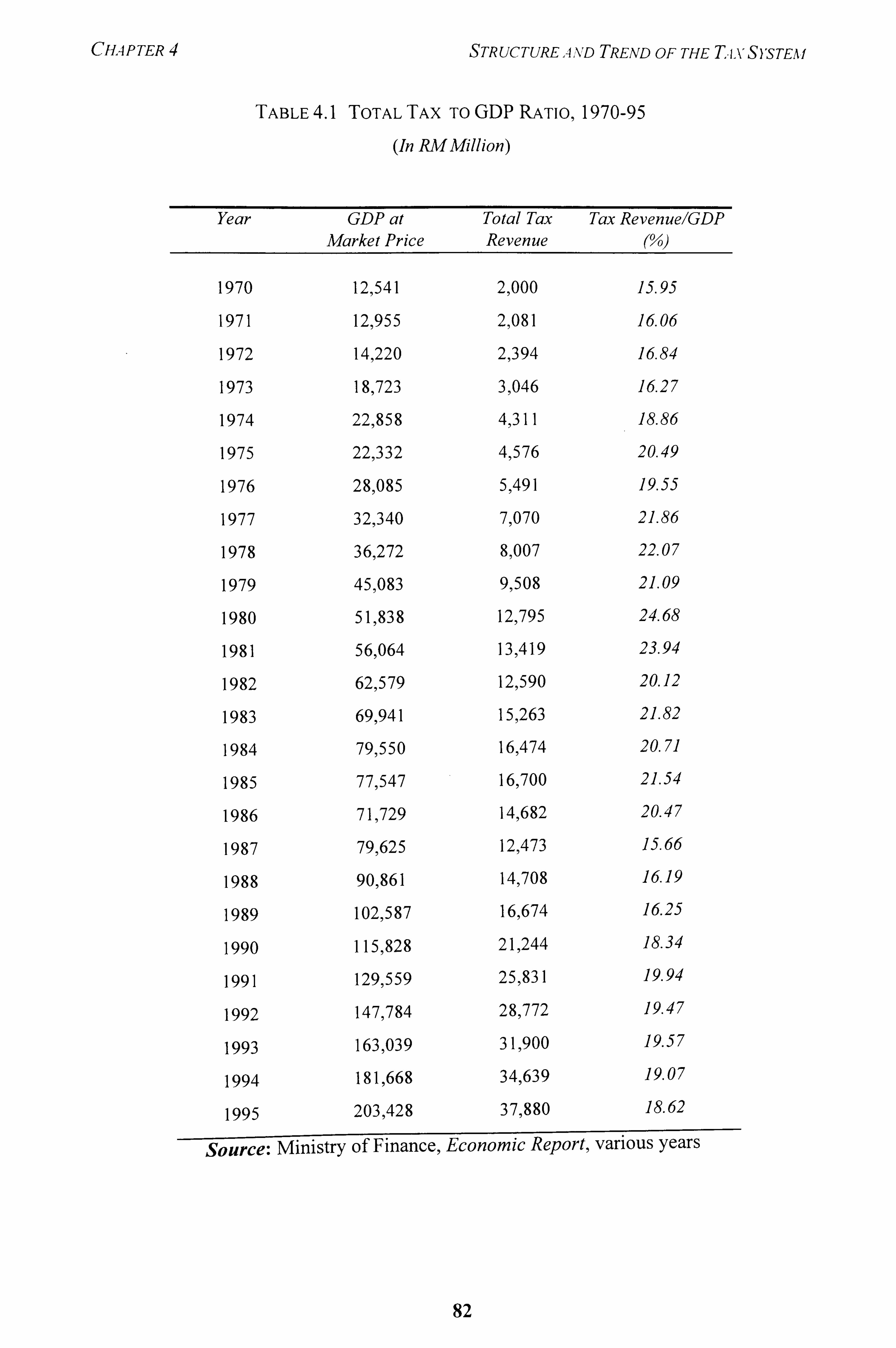
CRAP TER STRUCTUREAA"D TREND OF THE T-i, \, S)'STEA, f

TABLE 4.1 TOTAL TAX To GDP RATIO, 1970-95

(In RAII Million)

Year GDP at Total Tax Tax RevenuelGDP Market Price Revenue (0/0)

1970 12,541 2,000 15.95

1971 12ý955 2,081 16.06

1972 14ý220 2,394 16.84

1973 18,723 3,046 16.27

1974 22,858 4ý31 1 18.86

1975 22,332 4,576 20.49

1976 281085 5 ý491 19.55

1977 32,340 7ý070 21.86

1978 36,272 8,007 22.07

1979 45,083 9ý508 21.09

1980 51ý838 12ý795 24.68

1981 565064 13 ý419 23.94

1982 62,579 12ý590 20.12

1983 69,941 15ý263 21.82

1984 791550 16,474 20.71

1985 77,547 165700 21.54

1986 71 ý729 l4ffl2 20.47

1987 79,625 12,473 15.66

1988 90,861 14,708 16.19

1989 102,587 16ý674 16.25

1990 115ý828 211)244 18.34

1991 1291559 25ý831 19.94

1992 147ý784 28ý772 19.47

1993 163,039 31,900 19.57

1994 1819668 345639 19.07

1995 203ý428 37,880 18.62

Source: Ministry of Finance, Economic Report, various years

82

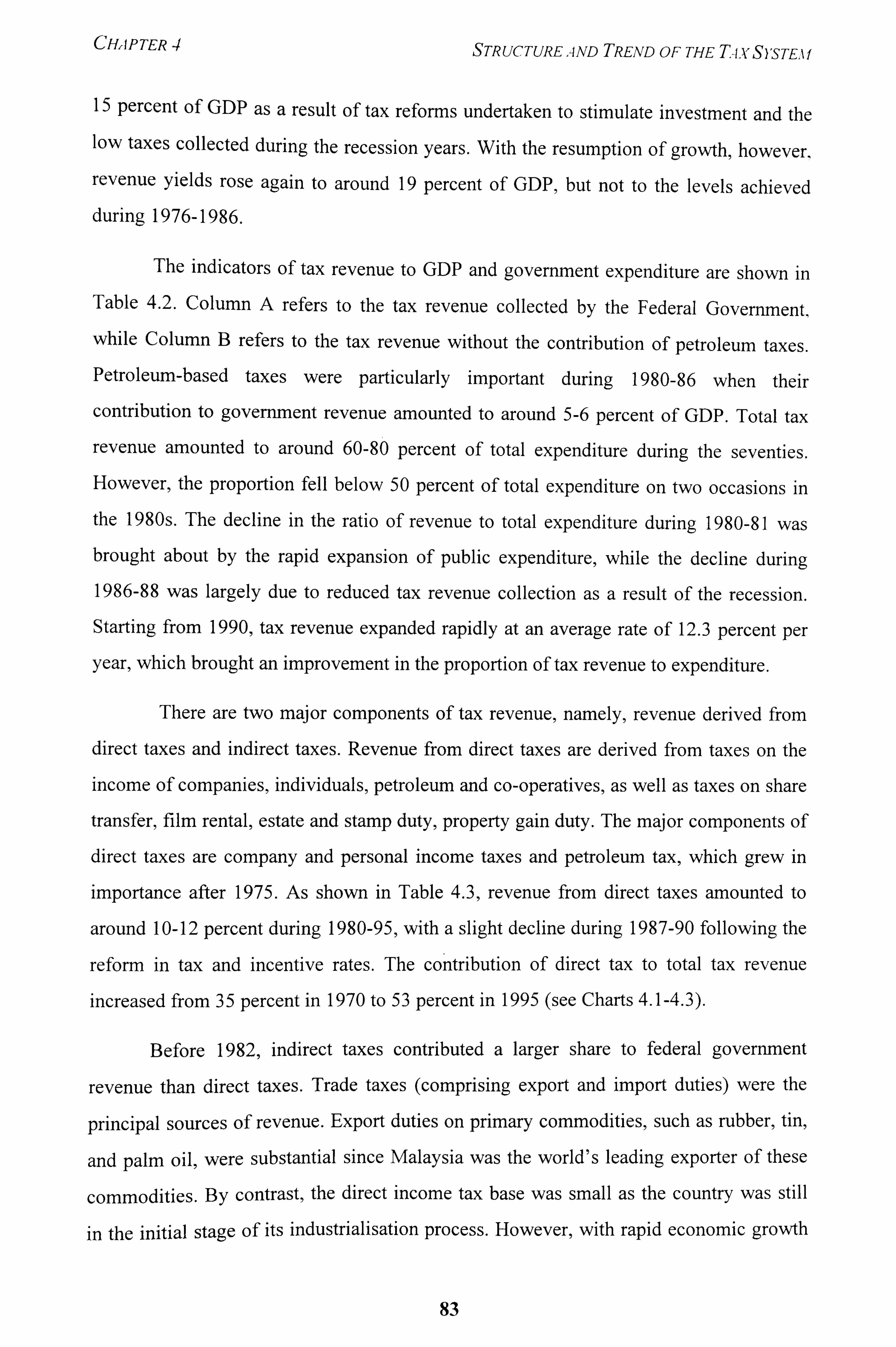
CHAPTER 4 STRUCTUREqND TREND OF THE T-i. vS), sTEM

15 percent of GDP as a result of tax reforms undertaken to stimulate investment and the low taxes collected during the recession years. With the resumption of growth, however.

revenue yields rose again to around 19 percent of GDP, but not to the levels achieved during 1976-1986.

The indicators of tax revenue to GDP and government expenditure are shown in Table 4.2. Column A refers to the tax revenue collected by the Federal Government.

while Column B refers to the tax revenue without the contribution of petroleum taxes. Petroleum-based taxes were particularly important during 1980-86 when their

contribution to government revenue amounted to around 5-6 percent of GDP. Total tax

revenue amounted to around 60-80 percent of total expenditure during the seventies. However,, the proportion fell below 50 percent of total expenditure on two occasions in the 1980s. The decline in the ratio of revenue to total expenditure during 1980-81 was brought about by the rapid expansion of public expenditure, while the decline during

1986-88 was largely due to reduced tax revenue collection as a result of the recession. Starting from 1990, tax revenue expanded rapidly at an average rate of 12.3 percent per

year, which brought an improvement in the proportion of tax revenue to expenditure.

There are two major components of tax revenue, namely, revenue derived from

direct taxes and indirect taxes. Revenue from direct taxes are derived from taxes on the

income of companies, individuals, petroleum and co-operatives, as well as taxes on share

transfer, film rental, estate and stamp duty, property gain duty. The major components of

direct taxes are company and personal income taxes and petroleum tax, which grew in

importance after 1975. As shown in Table 4.3, revenue from direct taxes amounted to

around 10-12 percent during 1980-95, with a slight decline during 1987-90 following the

reform in tax and incentive rates. The contribution of direct tax to total tax revenue

increased from 35 percent in 1970 to 53 percent in 1995 (see Charts 4.1-4.3).

Before 1982, indirect taxes contributed a larger share to federal government

revenue than direct taxes. Trade taxes (comprising export and import duties) were the

principal sources of revenue. Export duties on primary commodities, such as rubber, tin,

and palm oil, were substantial since Malaysia was the world's leading exporter of these

commodities. By contrast, the direct income tax base was small as the country was still

in the initial stage of its industrialisation process. However, with rapid economic growth

83

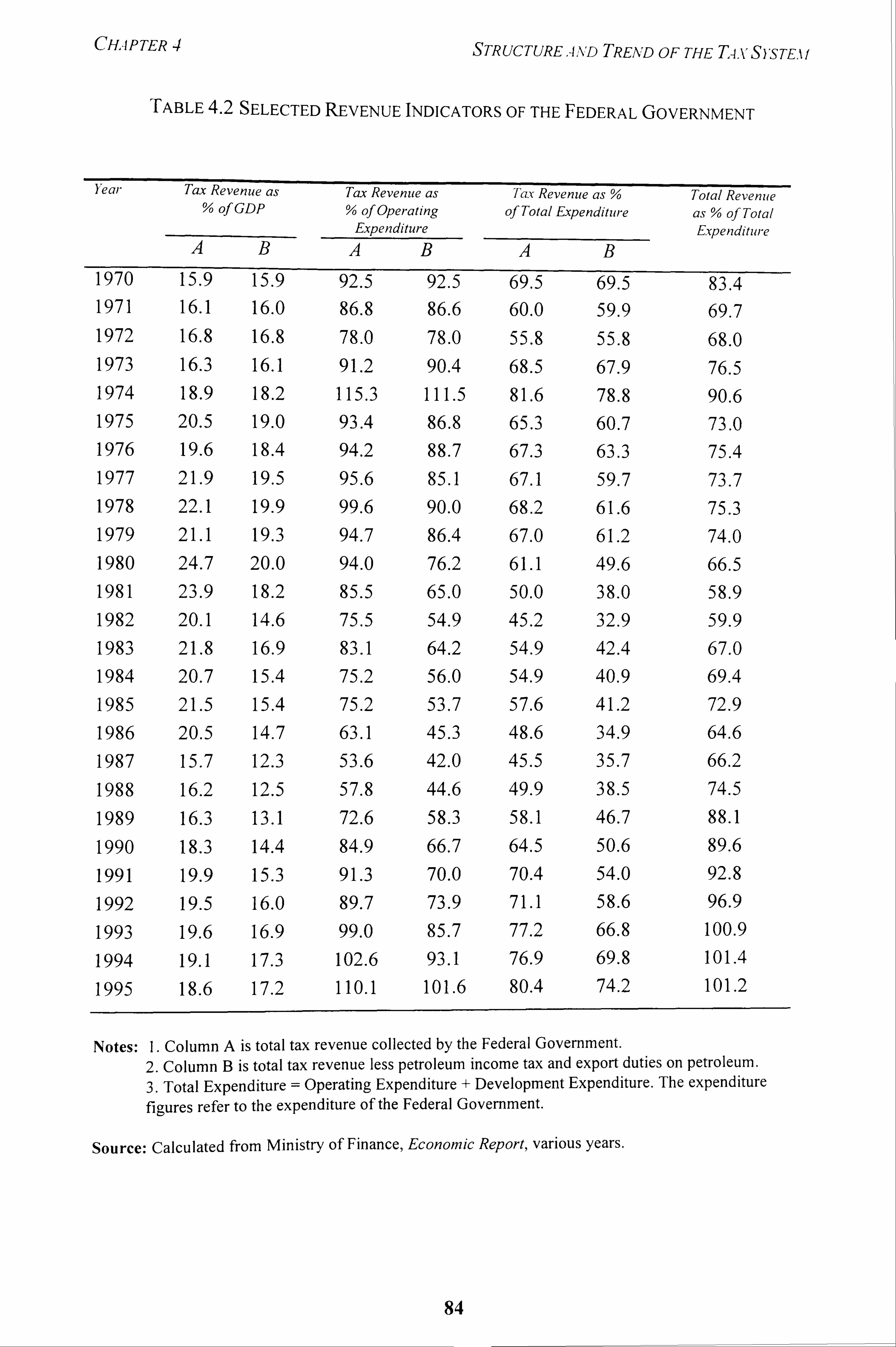
CHAPTER STRUCTURE, -i,, N, D TREA, ýD OF THE T4x S), sTE. i f

TABLE 4.2 SELECTED REVENUE INDICATORS OF THE FEDERAL GOVERNMENT

Year Tax Revenue as % of GDP

AB

Tax Revenue as % of Operating

Expenditure AB

Tay Revenue as % of Total Expenditure

AB

Total Revenue as % of Total Expenditure

1970 15.9 15.9 92.5 92.5 69.5 69.5 83.4 1971 16.1 16.0 86.8 86.6 60.0 59.9 69.7 1972 16.8 16.8 78.0 78.0 55.8 55.8 68.0 1973 16.3 16.1 91.2 90.4 68.5 67.9 76.5 1974 18.9 18.2 115.3 111.5 81.6 78.8 90.6 1975 20.5 19.0 93.4 86.8 65.3 60.7 73.0 1976 19.6 18.4 94.2 88.7 67.3 63.3 75.4 1977 21.9 19.5 95.6 85.1 67.1 59.7 73.7 1978 22.1 19.9 99.6 90.0 68.2 61.6 75.3 1979 21.1 19.3 94.7 86.4 67.0 61.2 74.0 1980 24.7 20.0 94.0 76.2 61.1 49.6 66.5 1981 23.9 18.2 85.5 65.0 50.0 38.0 58.9 1982 20.1 14.6 75.5 54.9 45.2 32.9 59.9 1983 21.8 16.9 83.1 64.2 54.9 42.4 67.0 1984 20.7 15.4 75.2 56.0 54.9 40.9 69.4 1985 21.5 15.4 75.2 53.7 57.6 41.2 72.9 1986 20.5 14.7 63.1 45.3 48.6 34.9 64.6 1987 15.7 12.3 53.6 42.0 45.5 35.7 66.2 1988 16.2 12.5 57.8 44.6 49.9 38.5 74.5

1989 16.3 13.1 72.6 58.3 58.1 46.7 88.1

1990 18.3 14.4 84.9 66.7 64.5 50.6 89.6

1991 19.9 15.3 91.3 70.0 70.4 54.0 92.8

1992 19.5 16.0 89.7 73.9 71.1 58.6 96.9

1993 19.6 16.9 99.0 85.7 77.2 66.8 100.9

1994 19.1 17.3 102.6 93.1 76.9 69.8 101.4

1995 18.6 17.2 110.1 101.6 80.4 74.2 101.2

Notes: 1. Column A is total tax revenue collected by the Federal Government. 2. Column B is total tax revenue less petroleum income tax and export duties on petroleum. 3. Total Expenditure = Operating Expenditure + Development Expenditure. The expenditure fiaUres refer to the expenditure of the Federal Government.

t: )

Source: Calculated from Ministry of Finance, Economic Report, various years.

84

CHAPTER 4 STRUCTUREAND TPEND OF THE TAXSYSTEA I

TABLE 4.3 DIRECT AND INDIRECT TAXES To GDP, 1970-95

(In RM Million)

Year Direct Tax Direct TaxlGDP Indirect Tax Indirect TaxlGDP Revenue (0/0) Revenue (0/0)

1970 701 5.59 1,299 10.36

1971 713 5.50 1,368 10.56

1972 801 5.63 1,593 11.20

1973 890 4.75 2,156 11.52

1974 1,384 6.05 2,927 12.81

1975 2,021 9.05 2,555 11.44

1976 2,167 7.72 3,324 11.84

1977 2ý946 9.11 4,124 12.75

1978 3,323 9.16 4,684 12.91

1979 31888 8.62 51620 12.47

1980 5ý664 10.93 75131 13.76

1981 6ý328 11.29 75091 12.65

1982 65405 10.24 6,185 9.88

1983 7,712 11.03 7,551 10.80

1984 8,445 10.62 85029 10.09

1985 9,259 11.94 7ý441 9.60

1986 8,653 12.06 6,029 8.41

1987 6,467 8.12 6ý006 7.54

1988 7ý509 8.26 7,199 7.92

1989 7,793 7.60 85881 8.66

1990 1 Oý402 8.98 10,842 9.36

1991 13,251 10.23 12,580 9.71

1992 15,403 10.42 13,369 9.05

1993 175070 10.47 14,830 9.10

1994 181533 10.20 16ý 106 8.87

1995 205186 9.92 l7fi94 8.70

Source: Calculated from Ministry of Finance, Economic Report, various years

85

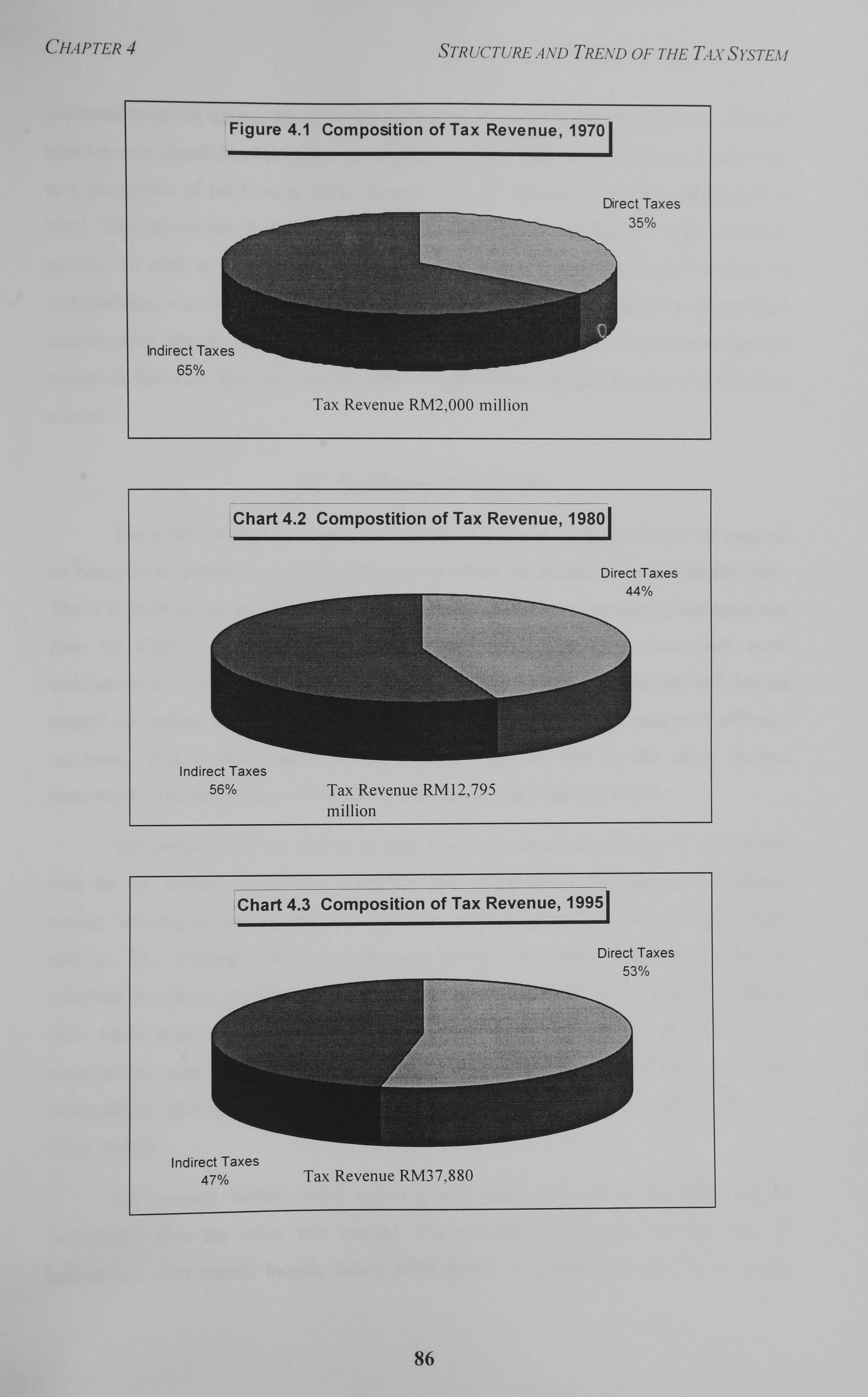
CHAP TER STRUCTUkE. 4. A, TD TREND OF THE T4-VS)STE, ll

Chart 4.2 Compostition of Tax Revenue, 1980 1

Direct Taxes 44%

Indirect Taxes 56% Tax Revenue RM 12,795

million

: Chart 4.3 Composition of Tax Revenue, 1995

Direct Taxes 53%

Indirect Taxes 47% Tax Revenue RM37,880

86

CHAPTER 4 STRUCTURE AND TREND OF THE T-ix S)'STE. ý f

and modernisation during the seventies and eighties, the contribution of indirect taxes to total revenue shrank in importance relative to the contribution of direct taxes. Trade taxes as a proportion of total tax revenue declined from 41 percent in 1970 to 18 percent in 1995. This shows the declining importance of primary commodities in total economic activity as well as the effects of the reduction in tariff rates and export duties on commodities. Furthermore, despite the rapid growth of commercial activities and private consumption, the contribution of sales, service and excise taxes to total revenue has not moved in the same direction, but declined in recent years, suggesting the need for a tax

reform.

2.1 Incidence of Taxation

The earlier studies on taxation in Malaysia focused on the incidence of taxation

on households, which is examining the way in which the burden of tax eventually falls.

The first study on the distribution of tax burden in 1957-58 for Peninsular Malaysia was

done by Charles E. McLure J. R. Subsequently, D. R. Snodgrass undertook some

estimations for 1968 and Ismail Muhd. Salleh for 1973. The three studies showed that the

overall tax structure in Peninsular Malaysia exhibited the U-shaped pattern of effective

tax rates, with greater burden falling on the lower as well as the upper income

households. The tax burden on middle income group was relatively lower.

The estimates of tax incidents were based on some assumptions of who would

bear the tax burden and by how much for each of the taxes. The income distribution

among households for a particular year was obtained from income and expenditure

surveys. The existing taxes were allocated among the income brackets in order to

calculate the pattern of effective tax burden. In the allocation of taxes, some assumptions

were made about the shifting of the tax burden on the income groups. Since these

assumptions were not based on empirical findings of the tax burden but on a priori

assumptions, incidence estimates of various taxes between the three studies could vary

fairly widely.

For instance, Salleh (1980) shows greater regressivity of the tax rates on poor

households than the other two studies. The estimate of the effective tax rate for

households with annual income below RMI, 800 is at a high 47.8 percent in Salleh,

87

CHAPTER 4 STRUCTURE AND TREND OF THE TA, k, S), sTE, ýf

compared with 19.9 percent in McLure (1972) and 31.2 percent in Snodgrass (1974). On the other hand, Snodgrass finds that tax progression appears to be most pronounced for households in the higher income brackets. His estimate of the effective tax rate for households with annual income above RM12,000 is 50.8 percent, compared with 40.0

percent in Salleh and 26.3 percent in McLure. The wide difference in the estimations

could only be partly attributed to changes in the estimates of income distribution and tax

structures between the years 1957-73. The other reason is the difference in assumptions

adopted in the studies regarding the shifting of the tax burden between

consumers/producers, exporters/importers, producers/distributors, as well as the income

groups adopted in each of the studies. The burden of taxes calculated should, therefore,

be taken as rough indications of the true patterns and be interpreted with some caution.

2.2 Tax Revenue in an International Context

Table 4.4 shows the contribution of various categories of taxes to total tax

revenue for groups of developing countries ranked by per capita GDP, as presented in

Tanzi (1987), which are compared with Malaysia's tax structure in 1980. With per capita

income of US$1,563, Malaysia falls within the US$850-1699 category of countries,

which acts as its reference group. The proportion of tax collection in GDP for Malaysia

(at 22.3 percent) was one and a half times higher than for the reference group. This was

because Malaysia derived a higher proportion of its taxes from foreign trade and income

and corporate taxes. As the world's leading exporter of rubber, tin, palm oil, and tropical

hardwoods, as well as petroleum, Malaysia received 20 percent of its tax revenues from

export duties and 16 percent from import duties in 1980. By comparison, the countries in

the reference group appear to be collecting a higher proportion of their tax revenues in

sales tax/VAT and excise duties.

Malaysia's revenue yield compares favourably with other middle-income East

Asian countries (Table 4.5). In terms of the ratio of tax revenue to GNP, Malaysia

collects more taxes than the other countries in the region. However, in 1989 the

difference in the ratio of tax revenue to GNP between Malaysia and countries such as

Thailand, Indonesia and South Korea is small, within the range of 0.3-1.3, percentage

points. In 1989, Malaysia's ratio of direct taxes to total revenue (at 30.8 percent) is

88

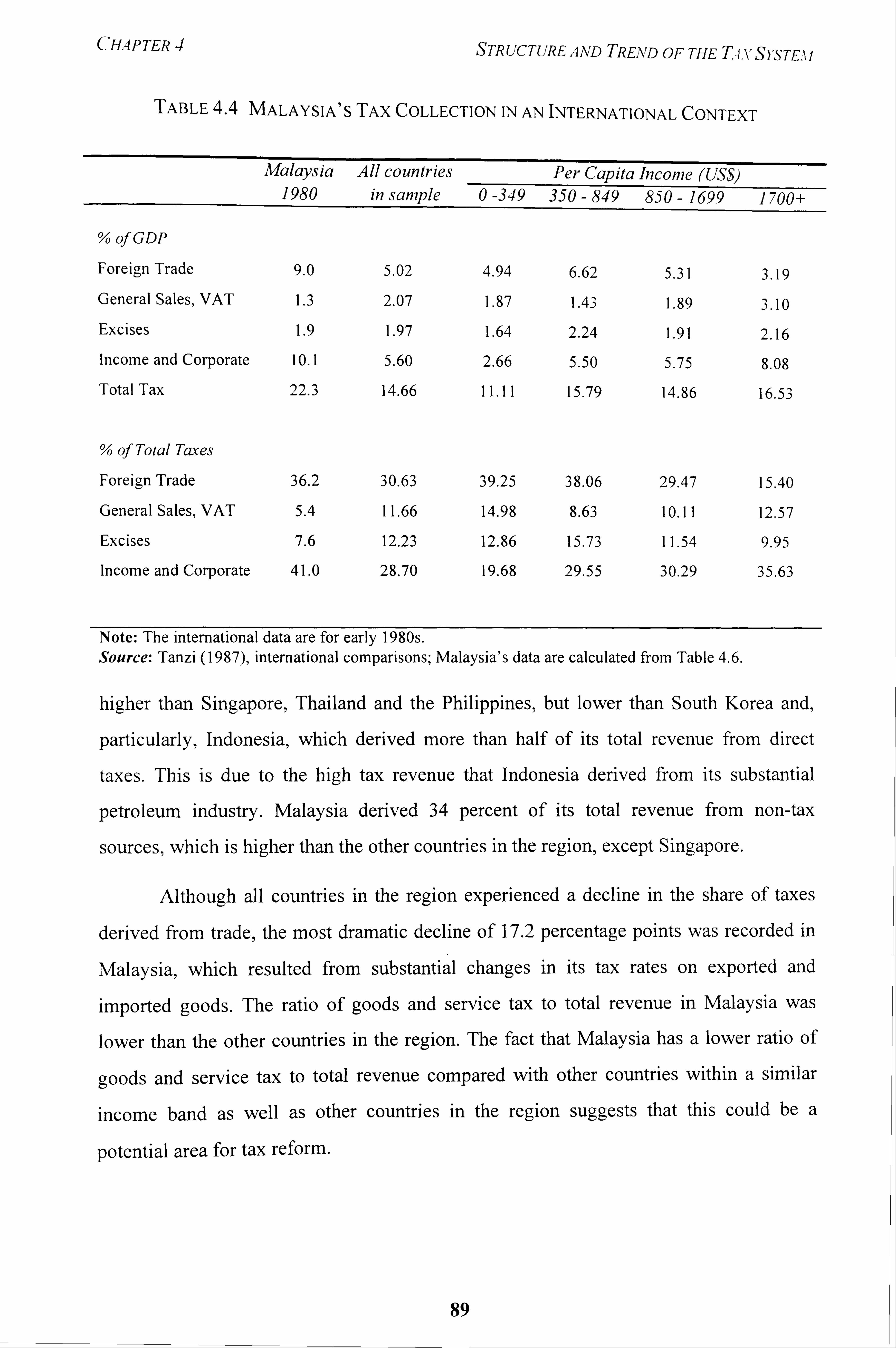
CHAP TER STRUCTUREAND TREND OF THE T-i, vS), sTEw

TABLE 4.4 MALAYSIA'S TAX COLLECTION IN AN INTERNATIONAL CONTEXT

Malaysia All countries Per Capita Income (USS) 1980 in sample 0-349 350-849 850-1699 1700+

% of GDP

Foreign Trade 9.0 5.02 4.94 6.62 5.31 3.19 General Sales, VAT 1.3 2.07 1.87 1.4 3 1.89 3.10

Excises 1.9 1.97 1.64 2.24 1.91 2.16

Income and Corporate 10.1 5.60 2.66 5.50 5.75 8.08

Total Tax 22.3 14.66 11.11 15.79 14.86 16-53 3

of Total Taxes

Foreign Trade 36.2 30.63 39.25 38.06 29.47 15.40

General Sales, VAT 5.4 11.66 14.98 8.63 10.11 12.57

Excises 7.6 12.23 12.86 15.73 11.54 9.95

Income and Corporate 41.0 28.70 19.68 29.55 30.29 35.63

Note: The international data are for early 1980s. Source: Tanzi (1987), international comparisons; Malaysia's data are calculated from Table 4.6.

higher than Singapore, Thailand and the Philippines, but lower than South Korea and,

particularly, Indonesia, which derived more than half of its total revenue from direct

taxes. This is due to the high tax revenue that Indonesia derived from its substantial

petroleum industry. Malaysia derived 34 percent of its total revenue from non-tax

sources, which is higher than the other countries in the region, except Singapore.

Although all countries in the region experienced a decline in the share of taxes

derived from trade, the most dramatic decline of 17.2 percentage points was recorded in

Malaysia, which resulted from substantial changes in its tax rates on exported and

imported goods. The ratio of goods and service tax to total revenue in Malaysia was

lower than the other countries in the region. The fact that Malaysia has a lower ratio of

goods and service tax to total revenue compared with other countries within a similar

income band as well as other countries in the region suggests that this could be a

potential area for tax reform.

89

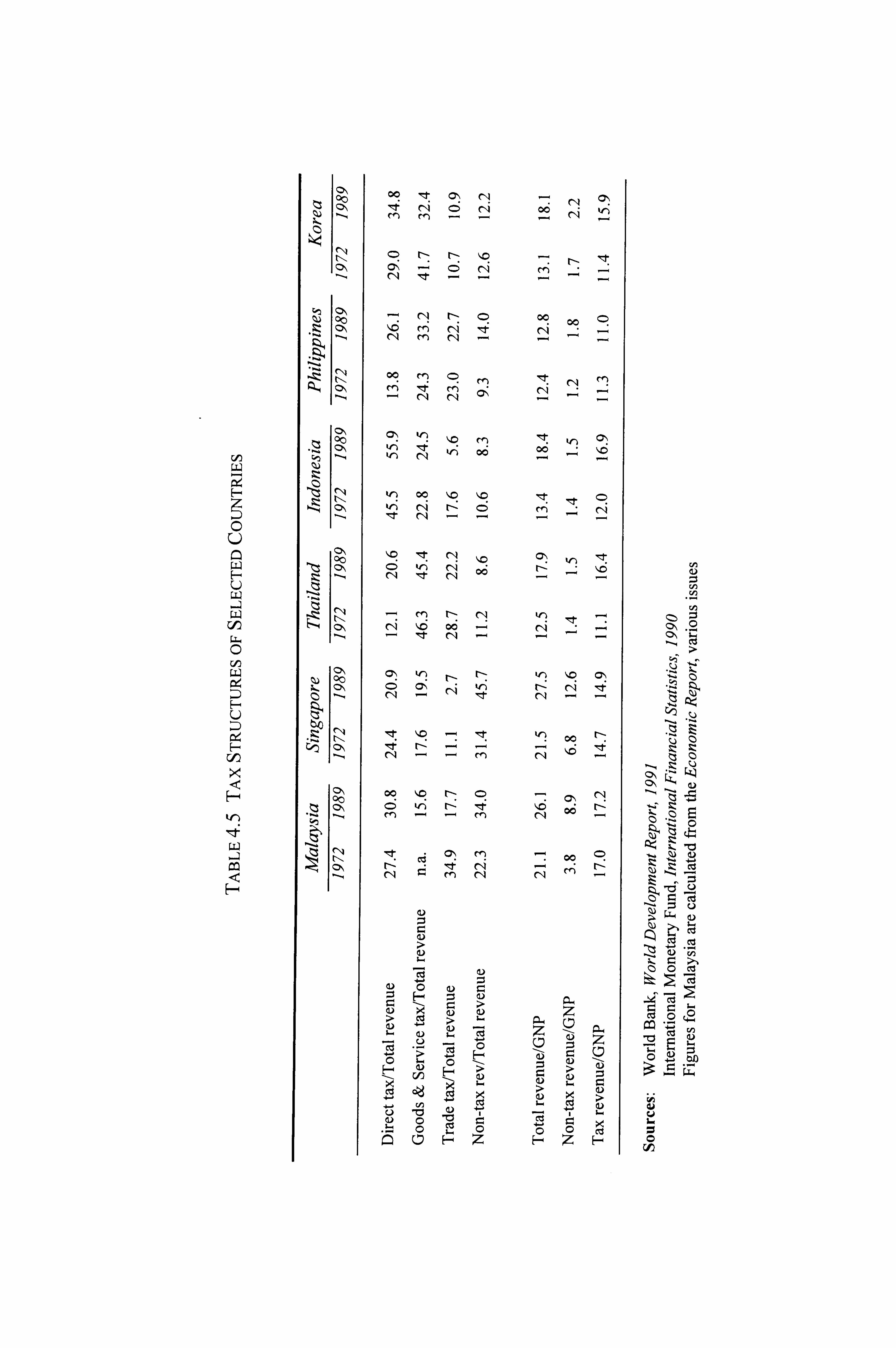
kn

t12 ru

.Z

Q.,

re Cu Z

$1 (Z

O\ CO cN\ rq rg Zý le

M rn CD -

CA oý rý

O\ a, ' - CD rq tý -ý -

00 r, -I m rq -

09 m cý , '11: (-q fn C> rn e rn C, 1

00 ýiD m kn C>

�zý rq 'rý 00

C> v-i N r-- CD rn _-; rq

(>ý cý krý rý oý r- �0 u

ý 6 d ON r \ý o rý ý> 2 le rl - --4 Z ýe

ý> cý cý cý vi t--: (-i le: rn

ru

1-1 r, 1 - - rn cq - ýI Z L

rn drr) rq - Z, Z E

rN t-, ,e cd

Cý oo eý , -

g-, r4) '+-

"C c) +ý

112: rý r, ý r- Z -0 CJ

Z r. ce

ru

C) > C, 2 cu

Z 0 (Z ýe zý c12

> 04 > >

-ý

X SZ X > u x (V

> N..

>< fi zm

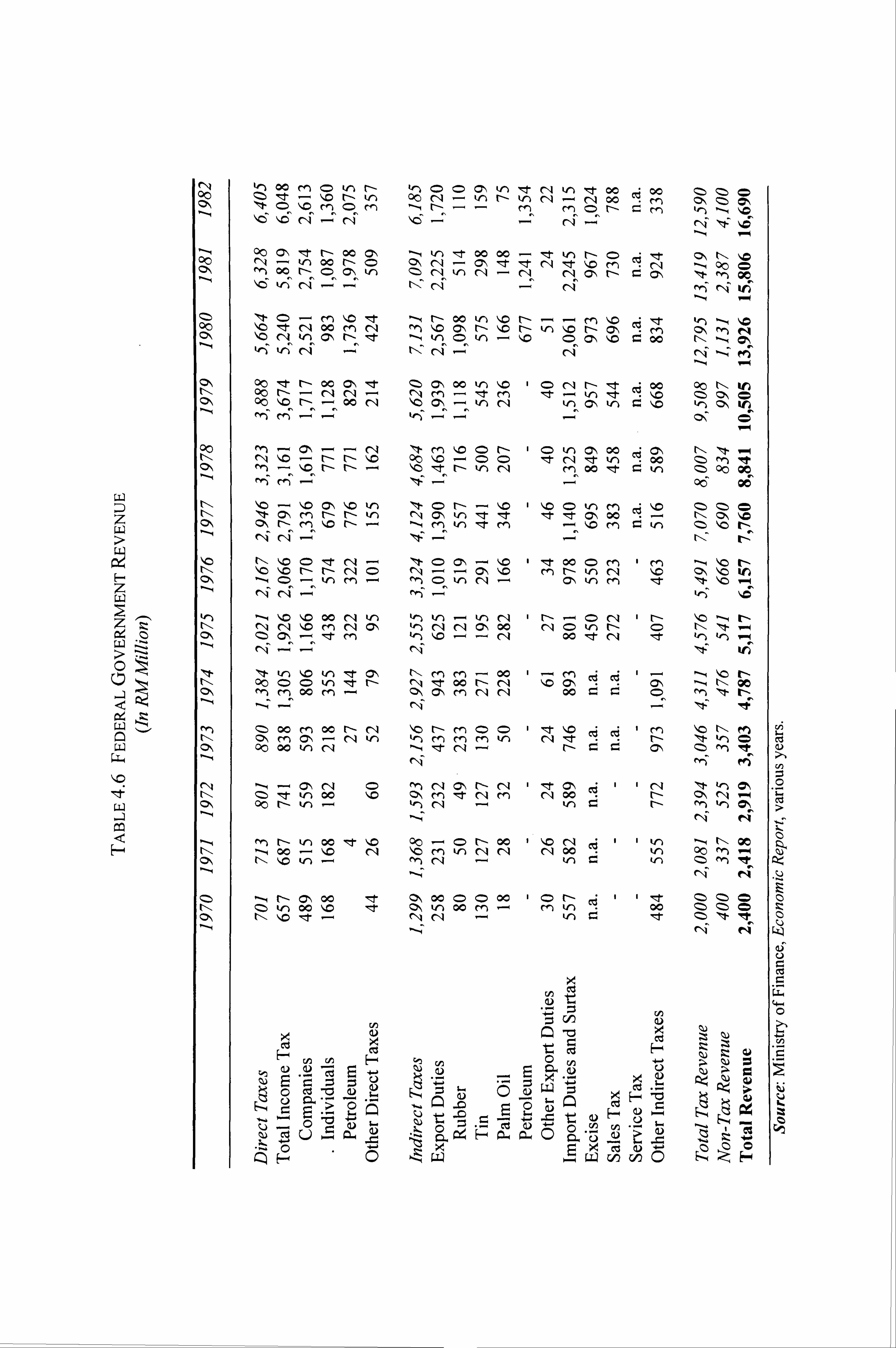
N -1 00 cn C) tn (-- qj- rl vi zt 00 00 Oo IZ tl- - ý, c r-- kn CC "- kn t-- kn ('q -ý C, 4 00 ct (Z (Z =

ON 'I- (:: ) so cn (= cn --4 t-- -- ci f1r) 0ý (Z) CIN mM Cý t-- m tn 114 ýz

ý16

r-- 00 tr) 00 00 00 ("ýl tf) oc r- c) C, 4 (7ý, 00 0ý "n 00 Cq I-t en 00 tn'

cn r- 00 tn rn "o C6 'tj-

oc \C) ýc CD C. ) 110 00 t, ý -" C; -ý

klý krý rli C'ý -ý clý en --4 W-4

ON r- 00 00 kn I'D I C) CA r-- "t C6 00 00 tl- kn tlý 00 r- -" C-A zt m It- - Ln Rzt. 110 <Z ON (= ON 00 \0 r- - 00 " kn " kr) Cý kn r- \0 kr) ON kn "14 fy-ý

kc C) r-- C4

?ýNI.

-C - r-- C-- "C \C - C) C) , I- CA zt kn . 00 (Z en It

0-1 ý'n - r- tn C14 00 lqt C kn ýz 00 00 1-4 - -ý 06 00

w ýD 'I- C) r- - \D I "o C) tr) t-I ", I- c, ' m r- r- kr) N CIN V) ýT "! t I: t ', I- C'ý 00 tl- ON ý=

ON 0ý r- fn Iýc r- - -*-q m kn ItT m-ý, c m r- kn C. 1) ýo r-

cq 'It C) C*) - Ic 00 (:: ) m t-I \0 \0 r- r- " c) N--a, \0 m r- kn CA Iýc ON \0 tn all,

2

1-11, t-I 1-4 so ýc 00 " kr) kl") kr) - tr) "I r- - C> "1 r- \0 ---4 t-

m rq (31-) ke) rq Clý 00 C) tn I! t r-4

ýt t, 'o tn a-m cn - 00 1- rn cd cd I- ---, ýc t- Cý t-ý 00 C) C) kn Itt rl- N Itt 00 r-- " ý10 Clý -- Cý -" t-, 00

0\ ý'n m 00 m- ON C-, (-) " CA ooC., r- C) en I- t- .<ý --4

C4 s't w '-, en (: z 00 m 00 tl- C*ll \0 t- m c) C: ý I "t ý, c 6 cd Im \0 t-, en o" m (7, -" kn kr) mmM kn rl- I- k-j = 00 kf) C14 CN <z cle) !! t

clq --I - (7ý C14 C) c1r) " (7ý r- "--,: I- a, :d-- C4 "It kn Cý 4 t-ý (Z) "! t kr) 00 I%D C>N m I- "m rq 00 - r- ON N V-0 kr) C14 1-4 kn kr) CIN

r- V) 00 tt \. o - C) (ý- 00 1 \C N :611 tf) -4 r, ot 00 - \C CIA M kf) " (114 " 00 - kn 00 en 9-4

rl- Cý 00 1171- 0ý 00 cý c, 00 - (:: ) r- Cý -- -'I- (Z (Z) 0 Zý W) 00 110 1- CN kn 00 tn 00 <Zý (Z) (Z

cq

C4 Q)

cz mxC., ;z 03 tz

-C, 0

Col. 'Z6) E 0 C-)

Llý .w un cn C) 1-; ýý F*

Z (Z

cl

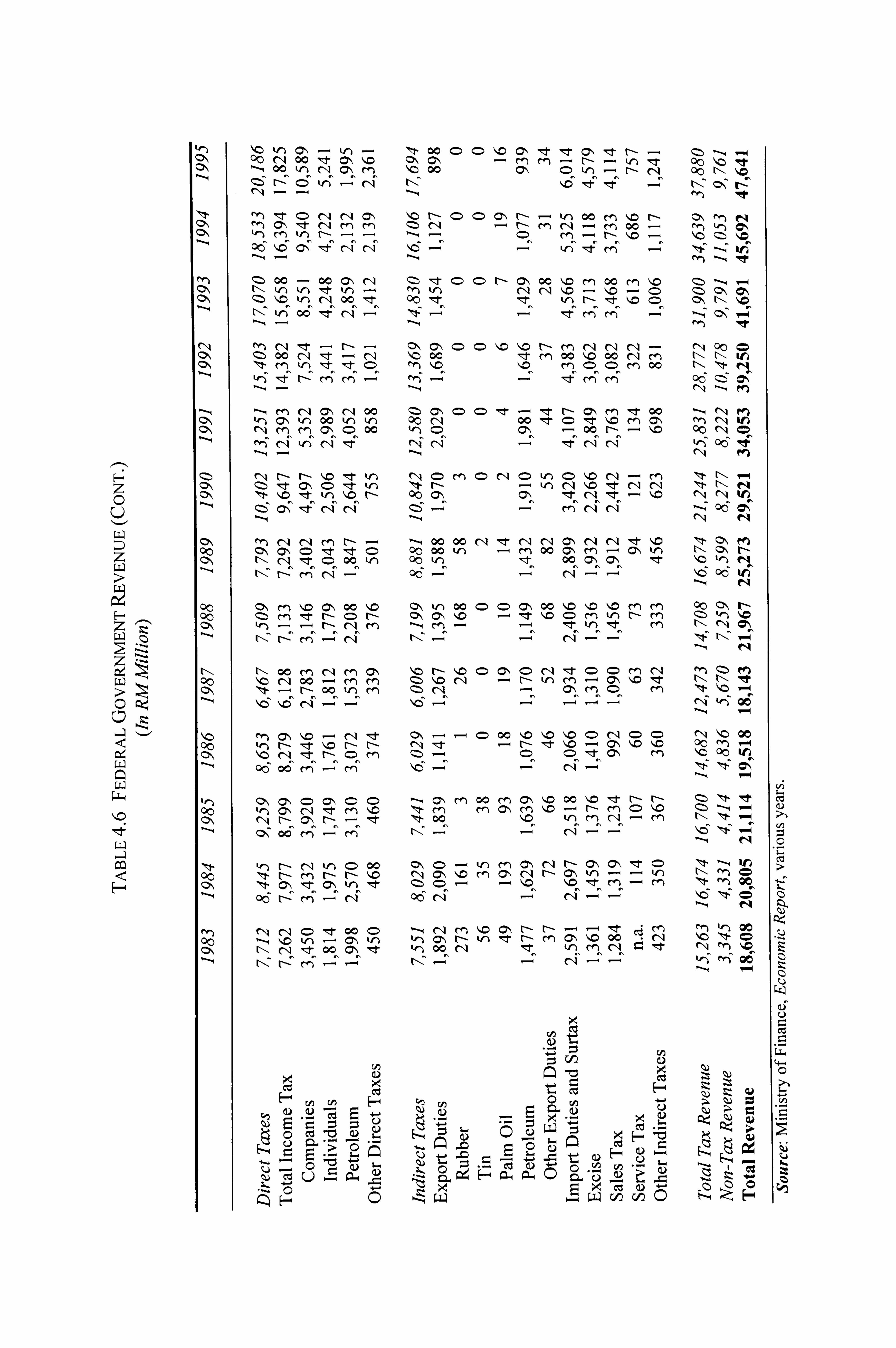
7 0 L)

z

z Lr -. 2-

LL

H

le) 0\ ON 1-4

m

en ON

('14 CN

ON 00

00 00

I r-ý Oo 011

ýo 00

kn 00 0\

P,

1 111- 00

1 en Oo ON

4

ýo 00

kr) C, 4

Cý 00 . "t

V-) C., - ,c

1- 0\ 00 (01,

C> (= INC -

CIN M

"ll M

*1- -

(7-1 r-

It -

r- - tl-

Cý) 00

---I \0 V-0

q1t 4 00 kr) C, -l Cý m \0 00 Cýl C) V) - clq 00 t, - ýz

clý qlý' q4' t-. 17 e cpý r-ý n qFt

en fn

I- clý

C) zt

" (-, I

" rn

CS, rn

\0 (Z

r-- C14

CD C) C', -

I-- r--

- cn

kr) rA

00 -

m rn

\0 00

r- -

ON en

en I-)

e4 a, \ ko'ý M W) r-

' - - ý-4 - (:: > en - r- ý, o - \0 <z ýz

Ile Cý llz: tf rlý C-ý lllý cn ---ý --m kK Wt

<z (-- 00

kr) - V*)

00 -1-

(Z en ZT

V-) C) C> t- C-,

cq 00 rq

\, c ýc

00 \0

"o C)

Zý (Z)

--4 ON

r" ON

(Z ý10 kn C14 00 00 It kn I, - Tt ýo C) trý oe q4' rlý rlý

00 CA zt - oc C) ý, c , ýc 't

[I- m

m 00

C'I \ýc

" 00

C14 C14

- m

00

C) C> 00 06 czý aN

N ---4 ef)

00 vi

00

V") 00 00 C) qtt \%c m

00

CS,

--

tn

N

N

en

kn

N m m (01, C) '

00 ke% C) C-\ - 00 r- - \%C) 00 N = -

llý 4 Clý - Lrý Clý lz: ý rq "-4 clý llzlý clý Cq t--ý N 06 Itt en

r-- I: t

r-- clýl

,: I- I: t

kn tr)

" I-

c:: ) r-

m Cý " C) -

ki") C> \C 1,0

" , 1-

- N

M "t "tt

I-, (--

T. -I eq

, '1- 110 Itt 110 r- 00 Cý CIN CA :t - N tq

06 ON

CN oll\ C> I: t I- C> 00 00 00

00 00 Cý

C', 4 rr)

C14 -

, I* C*)

"o kn

en t--

"t C: ) 00 kn 00 kn 00 CIN Cl\ It \C) e14 06 \6 06 kn-

ý'm C> 00 \Z et t- CD r--

(rý -- r- "m

t-lý tz rlý -ý, rý,

V) clý 00 \SO 110 ýc rn rn Cl\ mt ý, 0 CD rn (n r- rn

ý" le V_ý uz C'i -ý,

N ON

oo m (2, cli 00 rn - r-

rn Cý I'D - ('-I , I- kr, ) , I- 1ý0 r-- r- ýc Izi- r-- C)

06 oe rlý rlý

ON as, C) C*) C> C> kr) C*ý C14 Itt m Iýc N r- C*ý, r- - , I-

cpý oe r, ý ---ý r, ý

4-) r- clq ýn CD 00 'In- r- rn r- r- IZ 'le cý Imt

06 rz r, ý

00 C> Cý tr)

00 Cý It rz C, ý --ý --ý

C) 0 ce "0 (V

\C r- %0 (q le C> C) rn rý (Z2) \M (N rn - Cý 1,0 e (Z) rA Cý rn CD rn ý6 -ý, __r _r --r --:,

-- C> 00 %, C) \, O ým C> rý le - t-- et \Z - 0*ý

Itt O, \ rn

---q Cý m 00 m cl*N Iýc 00 1.0 ": t rl- (-- ', I- m cf) C\ m I'D - r'- en C) ý-c

00

C> C> - v-) m 01, (q r- cý, c> e CD v' \Z rq t-- alý (n --1. r) CD --4 \, CD ým e rn - rn

06 cý, --r r4 -ý, -ý, ---4 C'I m Ic ON t-- r-- -- tl- Cý rn tr) Cý kn It r- m (71, Iýc 00

ci C'4

kr) 00 kn rf)

X

Z -ci 9

'42 t4)

CD CD

en (Z-1) en

N 1%0 00 tn V. -O 00

-C

-4 00

rn W) 00 ýo ', I- (= N ýc

()i

ru Z.,

cz (1)

sz

:z Q t; n

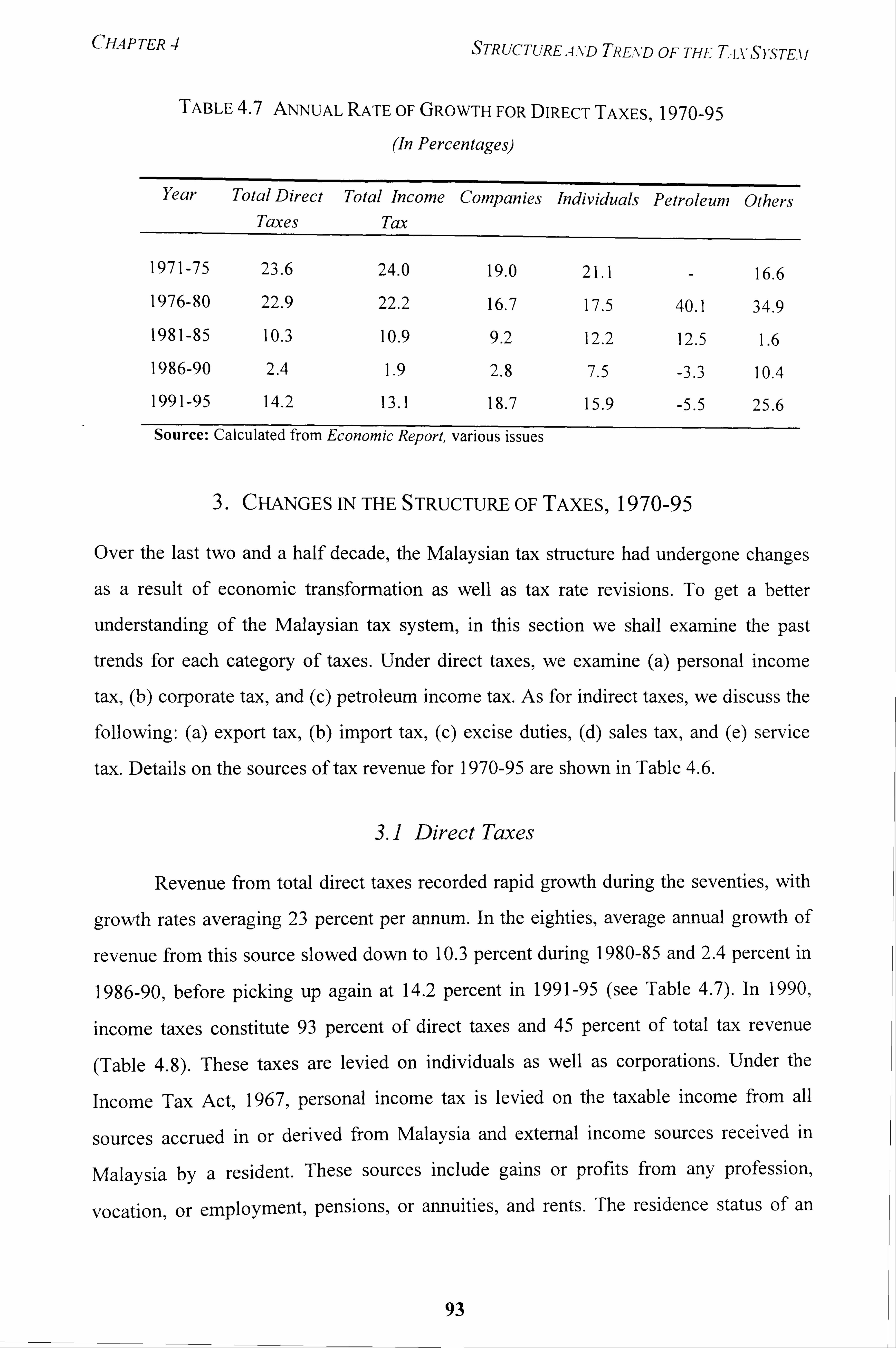
CHAPTER STRUCTUREAA'D TREND OF THE T-i, vS), sTEm

TABLE 4.7 ANNUAL RATE OF GROWTH FOR DIRECT TAXES, 1970-95

(In Percentages)

Year Total Direct Total Income Companies Individuals Petroleum Others Taxes Tax

1971-75 23.6 24.0 19.0 21.1 16.6 1976-80 22.9 22.2 16.7 17.5 40.1 34.9

1981-85 10.3 10.9 9.2 12.2 12.5 1.6

1986-90 2.4 1.9 2.8 7.5 -3.3 10.4

1991-95 14.2 13.1 18.7 15.9 -5.5 25.6

Source: Calculated from Economic Report, various issues

3. CHANGES IN THE STRUCTURE OF TAXES, 1970-95

Over the last two and a half decade, the Malaysian tax structure had undergone changes

as a result of economic transformation as well as tax rate revisions. To get a better

understanding of the Malaysian tax system, in this section we shall examine the past

trends for each category of taxes. Under direct taxes, we examine (a) personal income

tax, (b) corporate tax, and (c) petroleum income tax. As for indirect taxes, we discuss the

following: (a) export tax, (b) import tax, (c) excise duties, (d) sales tax, and (e) service

tax. Details on the sources of tax revenue for 1970-95 are shown in Table 4.6.

3.1 Direct Taxes

Revenue from total direct taxes recorded rapid growth during the seventies, with

growth rates averaging 23 percent per annum. In the eighties, average annual growth of

revenue from this source slowed down to 10.3 percent during 1980-85 and 2.4 percent in

1986-90, before picking up again at 14.2 percent in 1991-95 (see Table 4.7). In 1990,

income taxes constitute 93 percent of direct taxes and 45 percent of total tax revenue

(Table 4.8). These taxes are levied on individuals as well as corporations. Under the

Income Tax Act, 1967, personal income tax is levied on the taxable income from all

sources accrued in or derived from Malaysia and external income sources received in

Malaysia by a resident. These sources include gains or profits from any profession,

vocation, or employment, pensions, or annuities, and rents. The residence status of an

93

CHAPTER 4 STRUCTURE -I,, \D TREND OF THE T-ix S), sTE, t f

3 individual determines claims for personal relief and benefits of graduated rates . Company income tax is levied on the taxable income from all sources in Malaysia and income received from outside Malaysia for a resident company, and on income derived from Malaysia in the case of non-resident companies. Tax is levied for the preceding Year of Assessment (Y/A) ending on December 31.4

3. LI Personal Income Tax

The schedule of income tax rates for resident individuals is shown in Table 4.9. Individuals face progressive rates of taxes based on thirteen taxable income bands,, which

were reduced to nine following the 1995 Budget. Starting from the lowest chargeable income category, there are four bands of RM2,500 up to the chargeable income of RMIO, 000 and three bands of RM5,, 000 up to the chargeable income of RM25,000,

before larger increases in the chargeable income bands for individuals in the higher tax

categories.

Since the mid-1980s, the marginal tax rates for the highest and lowest taxable categories have been reduced in stages. In 1985 the top marginal tax rate was reduced from 55

percent to 40 percent, and subsequent reduction brought the top marginal tax rate to 32

percent in 1995. At the lowest taxable category, the marginal tax rate was brought down

from 6 percent to 5 percent in 1985 and subsequently to 3 percent in 1995, with the first

RM2,500 category of chargeable income exempted from tax. This cut in rates was meant

to encourage savings, although its effectiveness on savings has yet to be evaluated. The

effect of adjusting the top personal income tax rate on government revenue is minor,

notwithstanding the large reduction of marginal tax rate by 15 percentage points for the

top taxable income bracket. The share of personal income tax to tax revenue was

sustained at around 11-12 percent from 1982-92, before rising to 13.8 percent in 1995.

There is only a little fall in the share of personal income tax to tax revenue by 1.5

Non-resident employees are charged a flat income tax rate of 35 percent, subject to double tax treaty provisions. No personal reliefs are available to non-resident individuals.

4 Taxes for any Year of Assessment will be charged on the income of the preceding year.

94

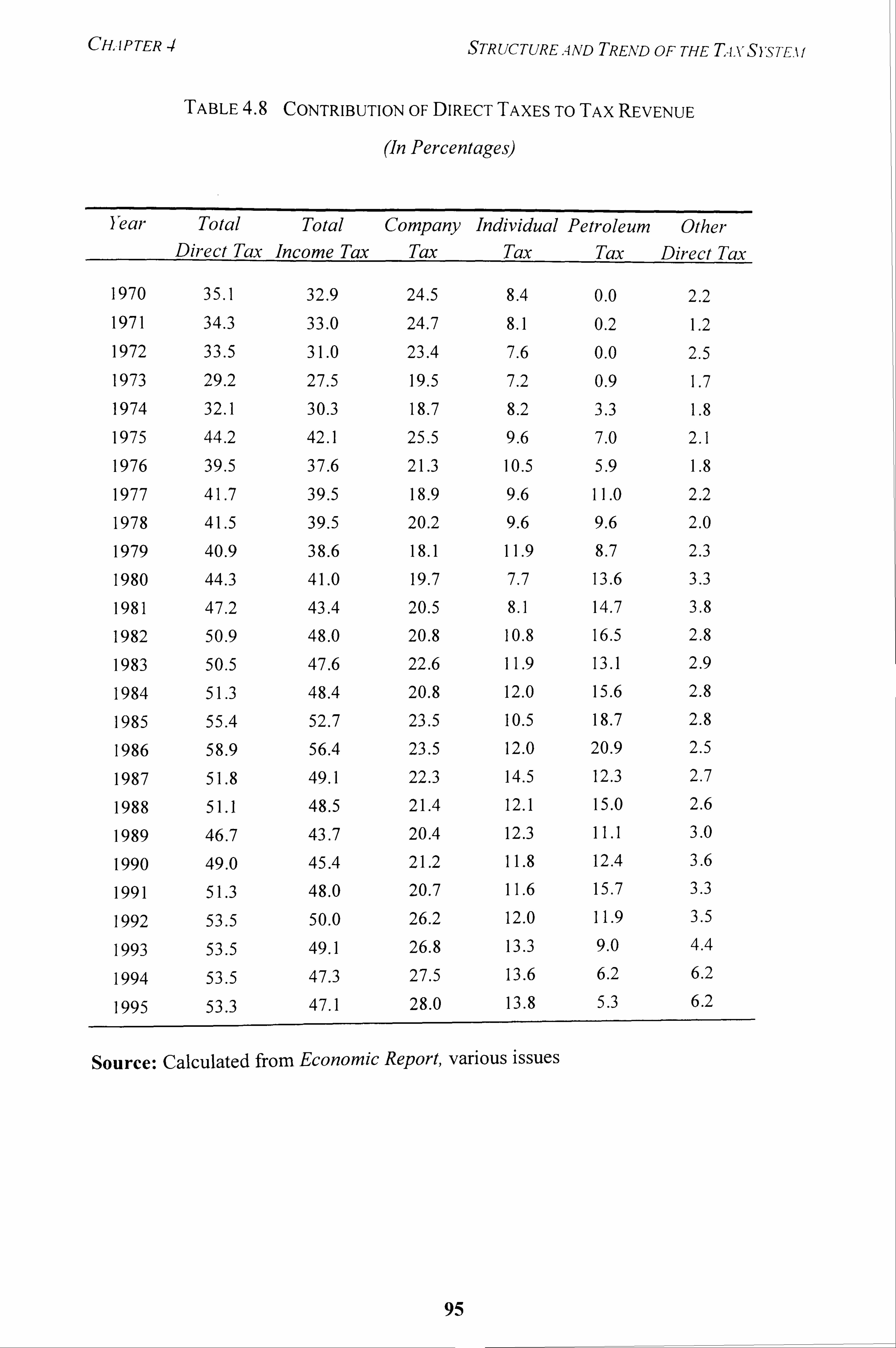
CHAPTER 4 STRUCTURE, 4ND TREArD OF THE TIVSYSTEAl

TABLE 4.8 CONTRIBUTION OF DIRECT TAXES To TAX REVENUE

(In Percentages)

Eear Total Direct Tax

Total Income Tax

Company Tax

Individual Tax

Petroleum Tax

Other Direct Tax

1970 35.1 32.9 24.5 8.4 0.0 2.2 1971 34.3 33.0 24.7 8.1 0.2 1.2 1972 33.5 31.0 23.4 7.6 0.0 2.5 1973 29.2 27.5 19.5 7.2 0.9 1.7 1974 32.1 30.3 18.7 8.2 3.3 1.8 1975 44.2 42.1 25.5 9.6 7.0 2.1 1976 39.5 37.6 21.3 10.5 5.9 1.8 1977 41.7 39.5 18.9 9.6 11.0 2.2 1978 41.5 39.5 20.2 9.6 9.6 2.0 1979 40.9 38.6 18.1 11.9 8.7 2.3 1980 44.3 41.0 19.7 7.7 13.6 3.3

1981 47.2 43.4 20.5 8.1 14.7 3.8

1982 50.9 48.0 20.8 10.8 16.5 2.8

1983 50.5 47.6 22.6 11.9 13.1 2.9

1984 51.3 48.4 20.8 12.0 15.6 2.8

1985 55.4 52.7 23.5 10.5 18.7 2.8

1986 58.9 56.4 23.5 12.0 20.9 2.5

1987 51.8 49.1 22.3 14.5 12.3 2.7

1988 51.1 48.5 21.4 12.1 15.0 2.6

1989 46.7 43.7 20.4 12.3 11.1 3.0

1990 49.0 45.4 21.2 11.8 12.4 3.6

1991 51.3 48.0 20.7 11.6 15.7 3.3

1992 53.5 50.0 26.2 12.0 11.9 3.5

1993 53.5 49.1 26.8 13.3 9.0 4.4

1994 53.5 47.3 27.5 13.6 6.2 6.2

1995 53.3 47.1 28.0 13.8 5.3 6.2

Source: Calculated from Economic Report, various issues

95

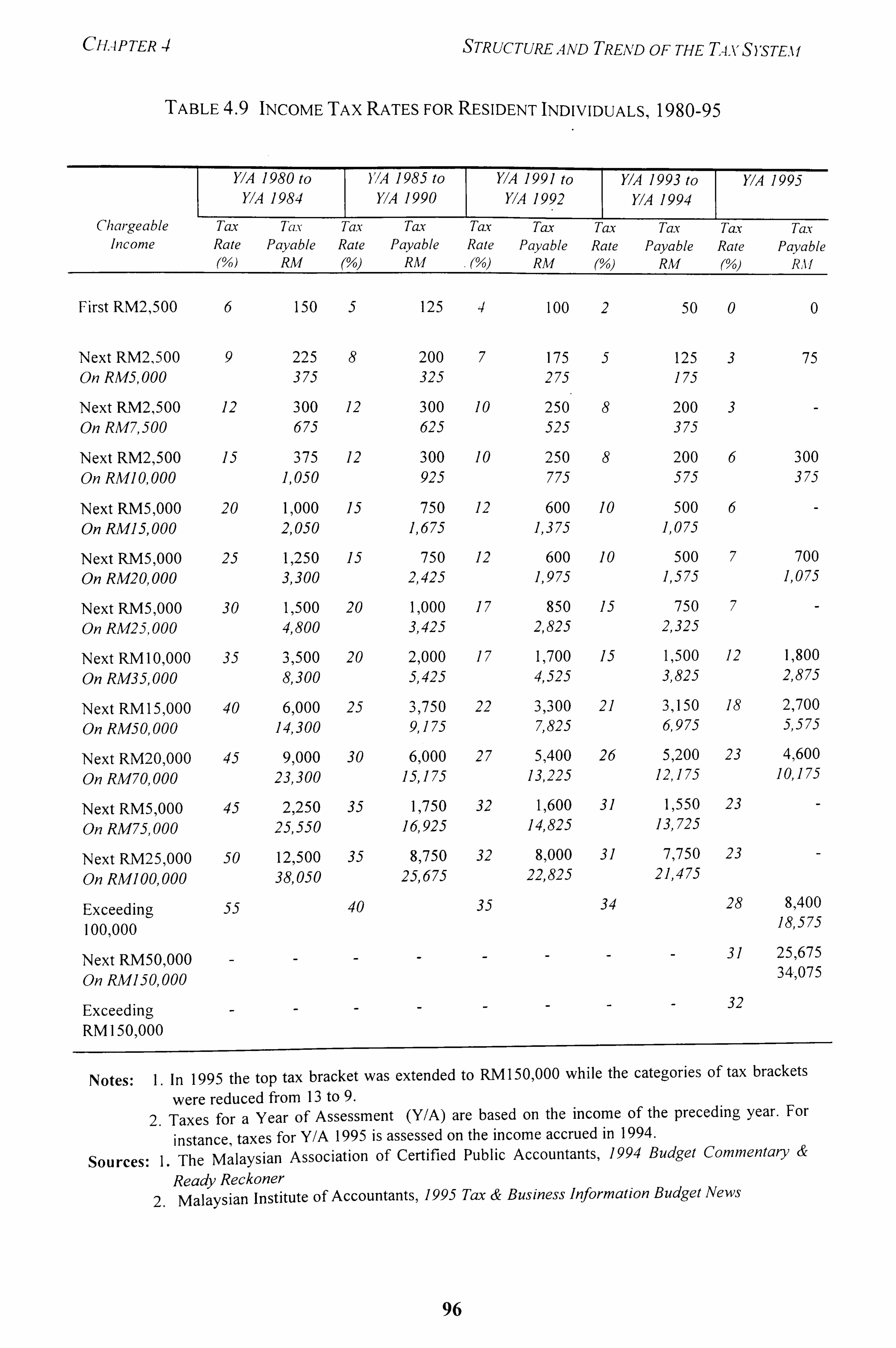
CHAPTER STRUCTURE, 4ND TREAD OF THE T4. VS)STE. If

TABLE 4.9 INCOME TAx RATES FOR RESIDENT INDIVIDUALS, 1980-95

YIA 1980 to YIA 1985 to YIA 1991 to YIA 1993 to YIA 1995 YIA 1984 YIA 1990 YIA 1992 YIA 1994

C hargeable I ax I ax I ax I ax I ax Tax Tax Tax TCLT Tax Income Rate Payable Rate Payable Rate Payable Rate Payable Rate Pq: vable

M RM C/o) R A/I (0/0) RM (0/0) RAf (0/0) RAI

First RM2,500 6 150 5 125 4 100 2 50 0 0

Next RM2,500 On RA15,000

Next RM2,500 On RA117,500

Next RM2,500 On RAIII 0,000

Next RM5,000 On RAI] 5,000

Next RM5,000 On RA1120,000

Next RM5,000 On RA1125,000

Next RM 10,000 On RM35,000

Next RM 15,000 On RAII50,000

Next RM20,000 On RA470,000

Next RM5,000 On RA1175,000


Exceeding 100,000


Exceeding RM 150,000

9 225 8 375

12 300 12 675

15 375 12 1,050

20 1,000 15 2,050

25 1,250 15 3,300

30 1,500 20 4,800

35 3,500 20 8,300

40 6,000 25 14,300

45 9,000 30 23,300

45 2,250 35 25,550

50 12,500 35 38,050

55 40

200 7 325

300 10 625

300 10 925

750 12 1,675

750 12 2,425

1,000 17 3,425

2,000 17 5,425

3,750 22 9,175

6,000 27 15,175

1,750 32 16,925

8,750 32 25,675

35

175 5 275

250 8 525

250 8 775

600 10 1,375

600 10 1,975

850 15 2,825

1,700 15 4,525

3,300 21 7,825

5,400 26 13,225

1,600 31 14,825

8,000 31 22,825

34

125 3 175

200 3 375

200 6 575

500 6 1,075

500 7 1,575

750 7 2,325

1,500 12 3,825

3,150 18 6,975

5,200 23 12,175

1,550 23 13,725

7,750 23 21,475

75

300 375

700 1,075

1,800 2,875

2,700 5,575

4,600 10,175

28 8,400 18,575

31 25,675 34,075

32

Notes: 1. In 1995 the top tax bracket was extended to RM 150,000 while the categories of tax brackets

were reduced from 13 to 9. 2. Taxes for a Year of Assessment (Y/A) are based on the income of the preceding year. For

instance, taxes for Y/A 1995 is assessed on the income accrued in 1994.

Sources: 1. The Malaysian Association of Certified Public Accountants, 1994 Budget Commentary &

Ready Reckoner 2. Malaysian Institute of Accountants, 1995 Tax & Business Information Budget News

96

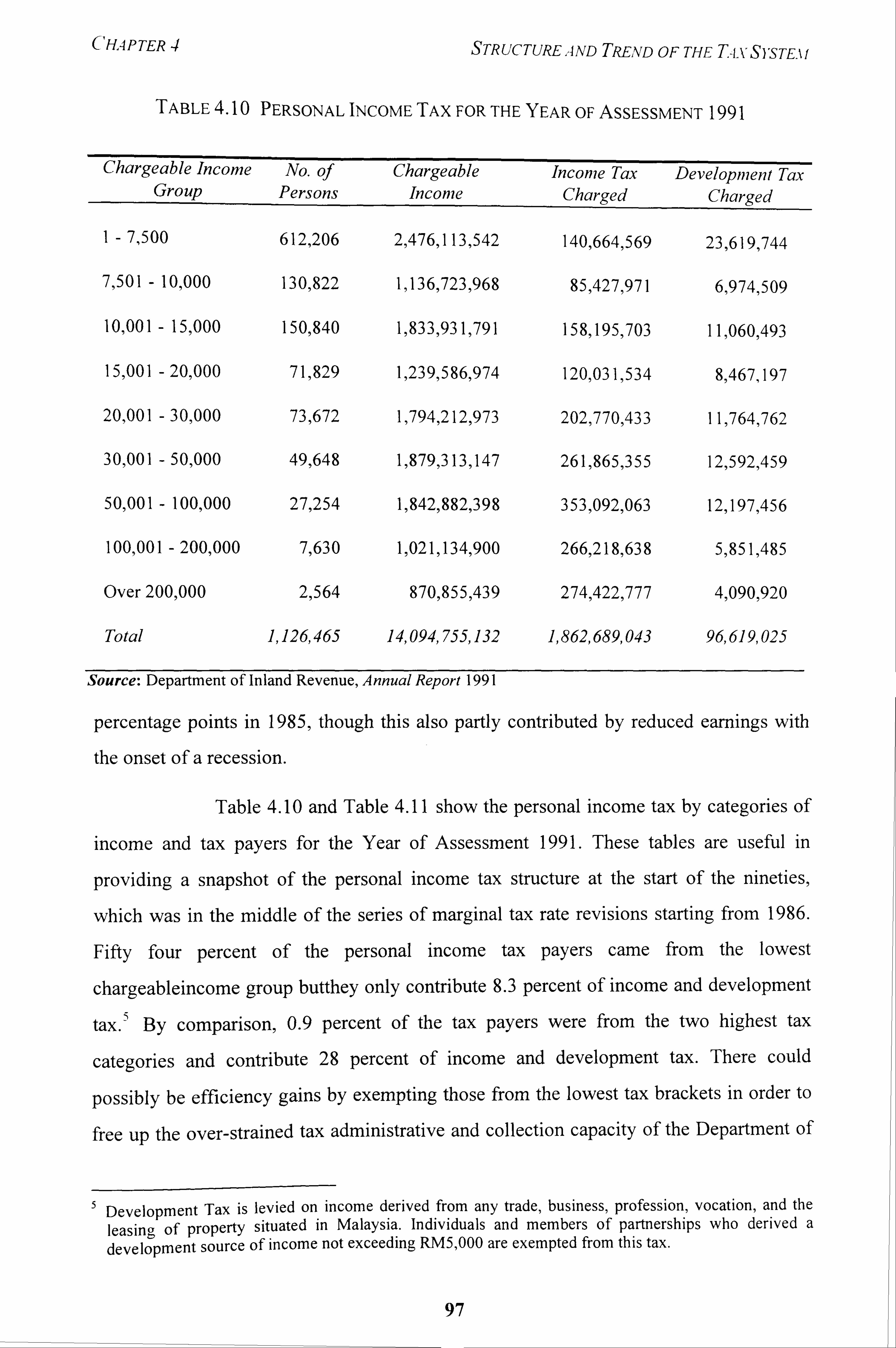
CHAP TER STRUCTURE., iND TREvD OF THE T-i-vS), sTEm

TABLE 4.10 PERSONAL INCOME TAX FOR THE YEAR OF ASSESSMENT 1991

Chargeable Income No. of Chargeable Income Tax Develo inent Tax p Group Persons Income Charged Charged

I-7,500 612,206 2,476,113,542 140,664,569 23,619,744

7,501 - 10,000 130,822 1,1 369723ý968 85,427,971 6,974,509

10,001 - 151,000 150,840 1,833,93 1,791 158ý 195,703 11,060,493

15,001 - 20ý000 71,829 1ý23%586,974 120,03 1 ý534 8,467,197

20,001 -30,000 73,672 1,794,2125973 202,770,433 11,764,762

30,001 -50,000 49,648 1,879,313,147 261,865,355 12,592,459

50ý00 1- 100,000 27,254 1,842,882,398 353,092,063 12,197,456

100,001 - 200,000 7,630 1,021,134,900 266ý2181638 5,851,485

Over 200,000 21564 87058555439 274,422ý777 4,090,920

Total 1,126,465 14,094,755,132 1,862,689,043 96,619,025

Source: Department of inland Revenue, Annual Report 1991

percentage points in 1985, though this also partly contributed by reduced earnings with

the onset of a recession.

Table 4.10 and Table 4.11 show the personal income tax by categories of

income and tax payers for the Year of Assessment 1991. These tables are useful in

providing a snapshot of the personal income tax structure at the start of the nineties,

which was in the middle of the series of marginal tax rate revisions starting from 1986.

Fifty four percent of the personal income tax payers came from the lowest

chargeableincome group butthey only contribute 8.3 percent of income and development

By comparison, 0.9 percent of the tax payers were from the two highest tax tax.,

categories and contribute 28 percent of income and development tax. There could

possibly be efficiency gains by exempting those from the lowest tax brackets in order to

free up the over-strained tax administrative and collection capacity of the Department of

5 Development Tax is levied on income derived from any trade, business, profession, vocation, and the leasing of property situated in Malaysia. Individuals and members of partnerships who derived a development source of income not exceeding RM5,000 are exempted from this tax.

97

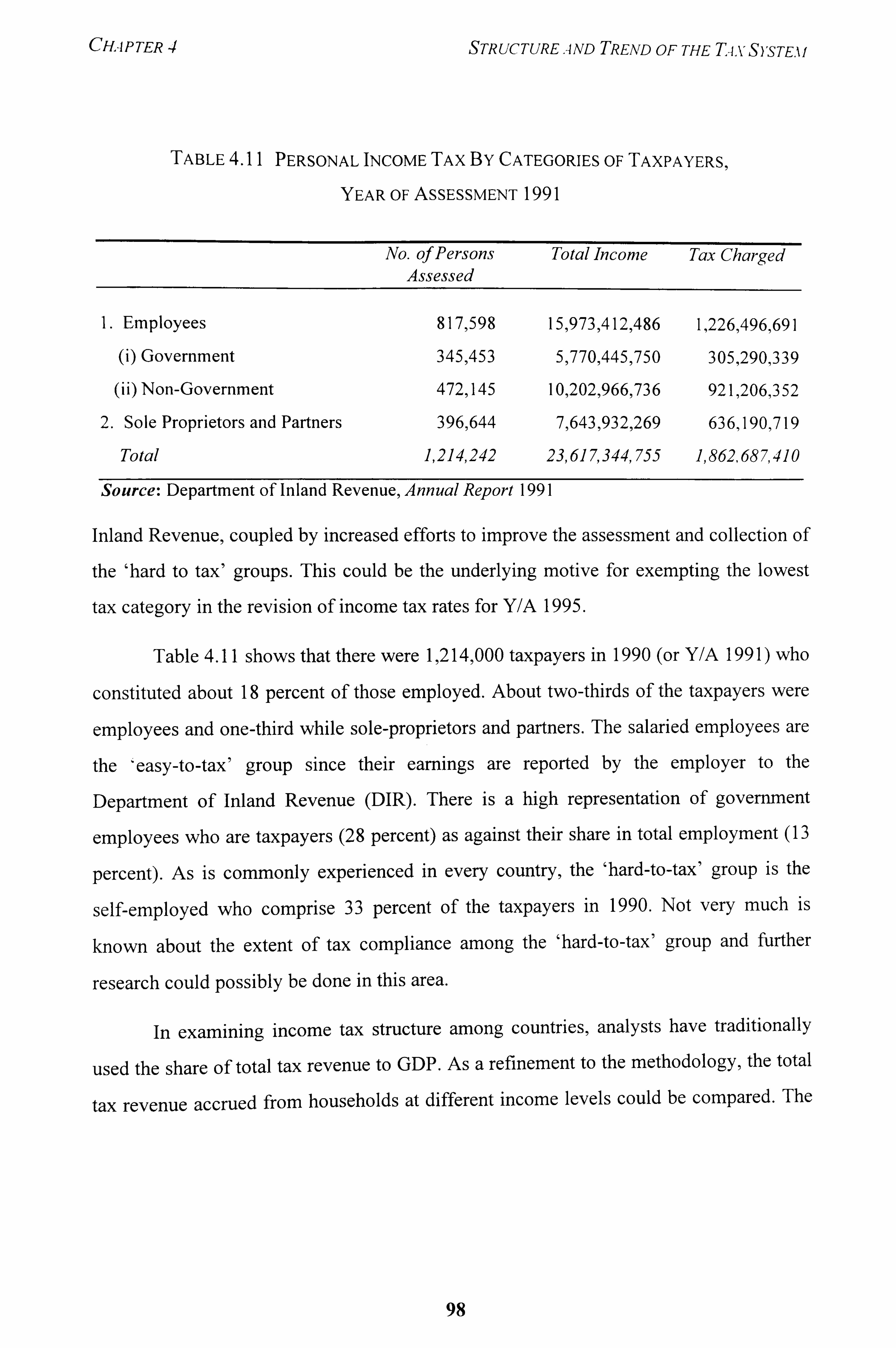
CHAPTER 4 STRUCTURE . 4ND TREND OF THE TIVSYSTEAl

TABLE4.11 PERSONAL INCOME TAX BY CATEGORIES OF TAXPAYERS,

YEAR OF AsSESSMENT 1991

No. of Persons Assessed

Total Income Tax Charged

1. Employees 817,598 151973ý412ý486 1,226,496,691

(i) Government 345,453 5,770,445,750 305,290,339

(ii) Non-Government 472ý 145 101202,966ý736 921,206,352

2. Sole Proprietors and Partners 3965644 7,643,9329269 636,190,719

Total 1,214,242 23,617,344,755 1,862,687,410

Source: Department of Inland Revenue, Annual Report 1991

Inland Revenue, coupled by increased efforts to improve the assessment and collection of

the 'hard to tax' groups. This could be the underlying motive for exempting the lowest

tax category in the revision of income tax rates for Y/A 1995.

Table 4.11 shows that there were 1 214,000 taxpayers in 1990 (or Y/A 199 1) who

constituted about 18 percent of those employed. About two-thirds of the taxpayers were

employees and one-third while sole-proprietors and partners. The salaried employees are

the 'easy-to-tax' group since their earnings are reported by the employer to the

Department of Inland Revenue (DIR). There is a high representation of government

employees who are taxpayers (28 percent) as against their share in total employment (13

percent). As is commonly experienced in every country, the 'hard-to-tax' group is the

self-employed who comprise 33 percent of the taxpayers in 1990. Not very much is

known about the extent of tax compliance among the 'hard-to-tax' group and further

research could possibly be done in this area.

In examining income tax structure among countries, analysts have traditionally

used the share of total tax revenue to GDP. As a refinement to the methodology, the total

tax revenue accrued from households at different income levels could be compared. The

98

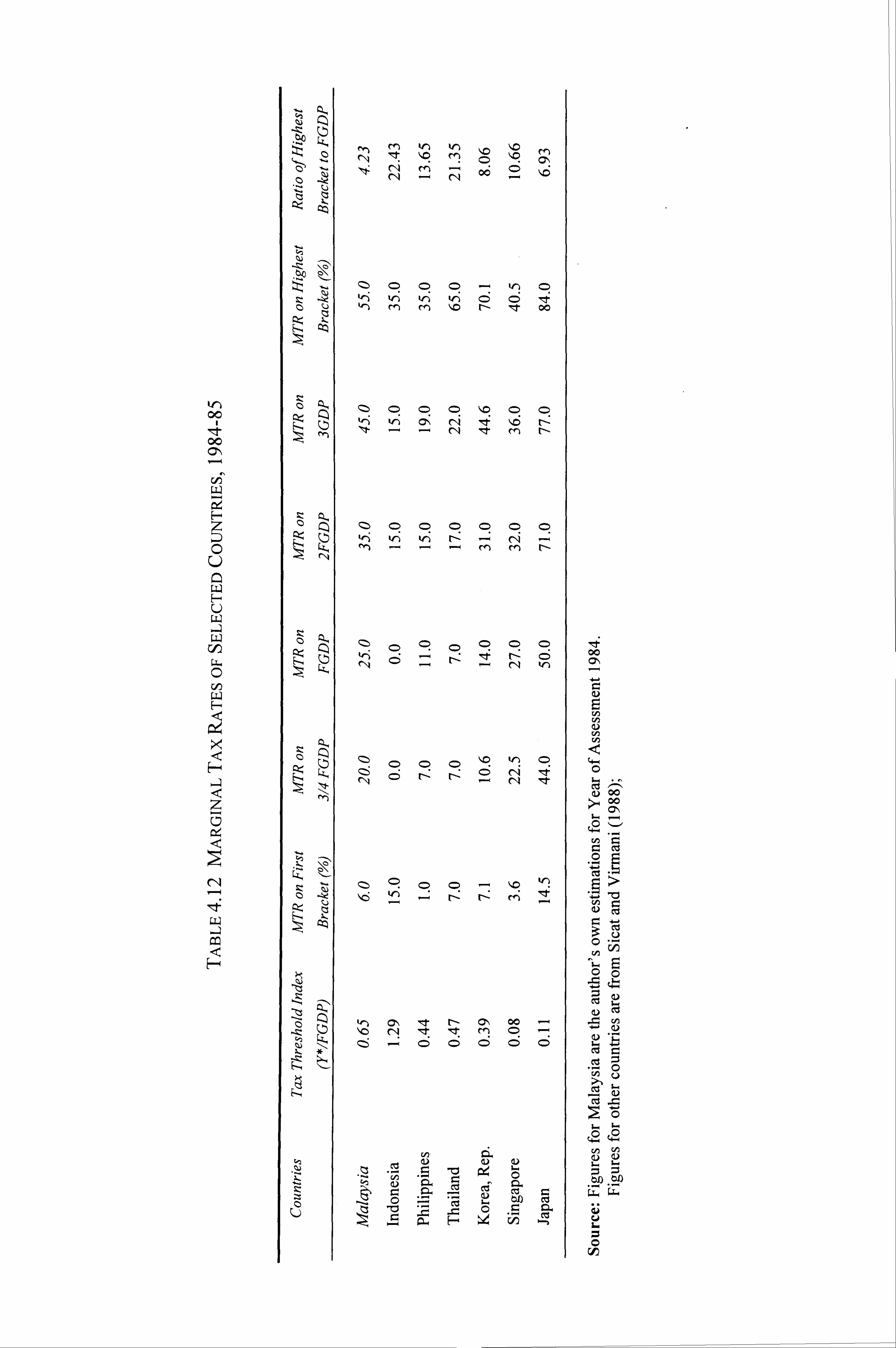
kn 00

4 00

-, Z (-ý

-Z "

z CL,

Z Z Z,

CLI

CQ

-Z

rn M V') kn "0 r11 Ilt \Z eM

CD

CD CD CD - kr) c>

klý vý krý cý cý le: rn rn \z r- le 00

Z) (=> c>

CD CD krý krý

rn r-ý ff) r--

Lr -N 'f

(Z) c>

z5 CD - �0 ý , ýý Irl -ý r-: r-: r, ý 'Z

Itt r- 00 C)

C5

rn - ýP e

e

.-

"a

5

cL CD-

--

e

m

pý

0

N..

r. CD.

4 00 (71,

E5

V) V)

(L) 00 oo

u2 r-

4ý ce ý;

-9 "a

ce =

I-.

C,, C, )

4.4. W

CHAPTER 4 STR UC TUREA ND TPEND OF THE TAx S), sTE. ý f

problem of focusing on the highest marginal rate is that it can give a misleading picture of the overall disincentives created by the tax system in a country. In this section, we adopt the approach introduced by Sicat and Virmani (1988) to compare the income tax base and the incentive effects of marginal tax rates among selected countries. We then

apply the same methodology to examine Malaysia's changing income tax rates over the

past 10 years.

For an average household, the method assumes a married couple with one income

earner and three children. To obtain the taxable income, we subtract from gross income

the standardised deductions and credits related to the family or linked to wage and salary

income. The country's 'one household GDP' (FGDP) is defined as five times per capita GDP. 6 The tax threshold index is calculated by taking the ratio of the threshold income

level over the one household GDP, i. e. Y*/FGDP. The numerator, Y* , is the income

threshold that is free from tax. It is equal to the income bracket that is free from tax plus

the basic exemptions. 7A zero tax threshold index means that all families, regardless of

their income level, will be taxed. If the value is 0.5, families with an income of less than

half FGDP are not subject to tax, while families with income equal to FGDP pay a tax

assessed on half their income. In other words, the greater the value of the index (arising

from larger deductions, credits, and zero bracket), the smaller would be the income tax

base.

Table 4.12 presents Malaysia's marginal tax rates (MTR) together with those of

Indonesia, Philippines, Thailand, the Republic of Korea, Singapore, and Japan. The

figures for Malaysia are our own estimates, while the figures for the other countries are

based on Sicat and Virmani. In 1984-85, Indonesia had an exceptionally high index

value,, where families having income equal to 1.3 times the FGDP were not taxed.

Indonesia's low tax base is consistent with the high administrative costs of collecting

taxes from a large, populous country comprising thousands of islands. Malaysia had the

next highest tax threshold index in view of the large tax relief given to income earners.

6 It is useful to note that this methodology tends to overestimate the average and marginal tax rates of developed countries since they typically have families of less than five. Although FGDP may

overestimate mean family income, this bias is not likely to distort the overall inter-country comparison.

7 For Malaysia, the tax free income bracket is RM2,500 before 1994 and RM5,000 after 1994. The

estimated personal relief of a family of five with a working husband, a non-working wife and three

children are RM 12,900 for 1984 and 1990, RM 13,900 for 1991 and 1993, and RM 15,400 for 1995.

100

CHAP TER 4 STR UCTURE, A ND TREND OF THE TA-V S)'STE. ý f

On the other hand, the threshold index for Singapore was very low, which was even lower than Japan. Its wide income tax base reflects the relative higher efficiency in

collecting taxes in an integrated city-state, island economy.

In the discussions on comparative tax rates among countries, analysts often focus

on the highest marginal tax rate since very high marginal tax rates are linked with the disincentives to work and save. Before drawing conclusions about the disincentive

effects on the basis of the highest tax rate among countries, it will be useful to ascertain

the size of the target group that falls within this tax bracket. In Table 4.12, the highest tax

brackets for Thailand (65 percent) and Indonesia (35 percent) only apply to families with income at more than 20 times the size of their FGDP. One can safely conclude that only

a tiny fraction of individuals fall within this tax category and even less would pay taxes

at this rate because of tax evasion. Another set of indicators is to examine the marginal

tax rate for those up to three times the size of FGDP. Families belonging to this income

bracket are in the upper middle class or the high income bracket. The table shows that the

Philippines, Thailand and Indonesia had the lowest marginal tax rates for households in

this category.

Among the neighbouring developing countries, Malaysian tax payers face the

highest marginal tax rates in 1984. Although the tax threshold index was high in

Malaysia, the highest tax brackets were reached very quickly. Individuals with family

income three-quarters the national average for one household GDP paid 20 percent taxes,

while those with three times FGDP paid 45 percent taxes. The highest tax bracket was

applied to those with income of more than 4.2 times FGDP. This bracket was reached

faster than the other developing countries in the table.

After comparing the tax structure of selected countries, we now examine the

progressivity of Malaysia's personal income tax. Table 4.13 presents the indicators of

progressivity calculated for 1984,1990,1991,1993 and 1995 using the methodology by

Sicat and Virmani (1988). The table shows that there had been considerable reform of

personal income tax in Malaysia during the last decade or so. The declining tax threshold

index shows that the tax base had been expanding over the years. In 1984 families with

incomes less than 65 percent of FGPD did not pay taxes. The tax net was wider a decade

later; only those with family income less than 44 percent of FGDP were tax exempted.

101

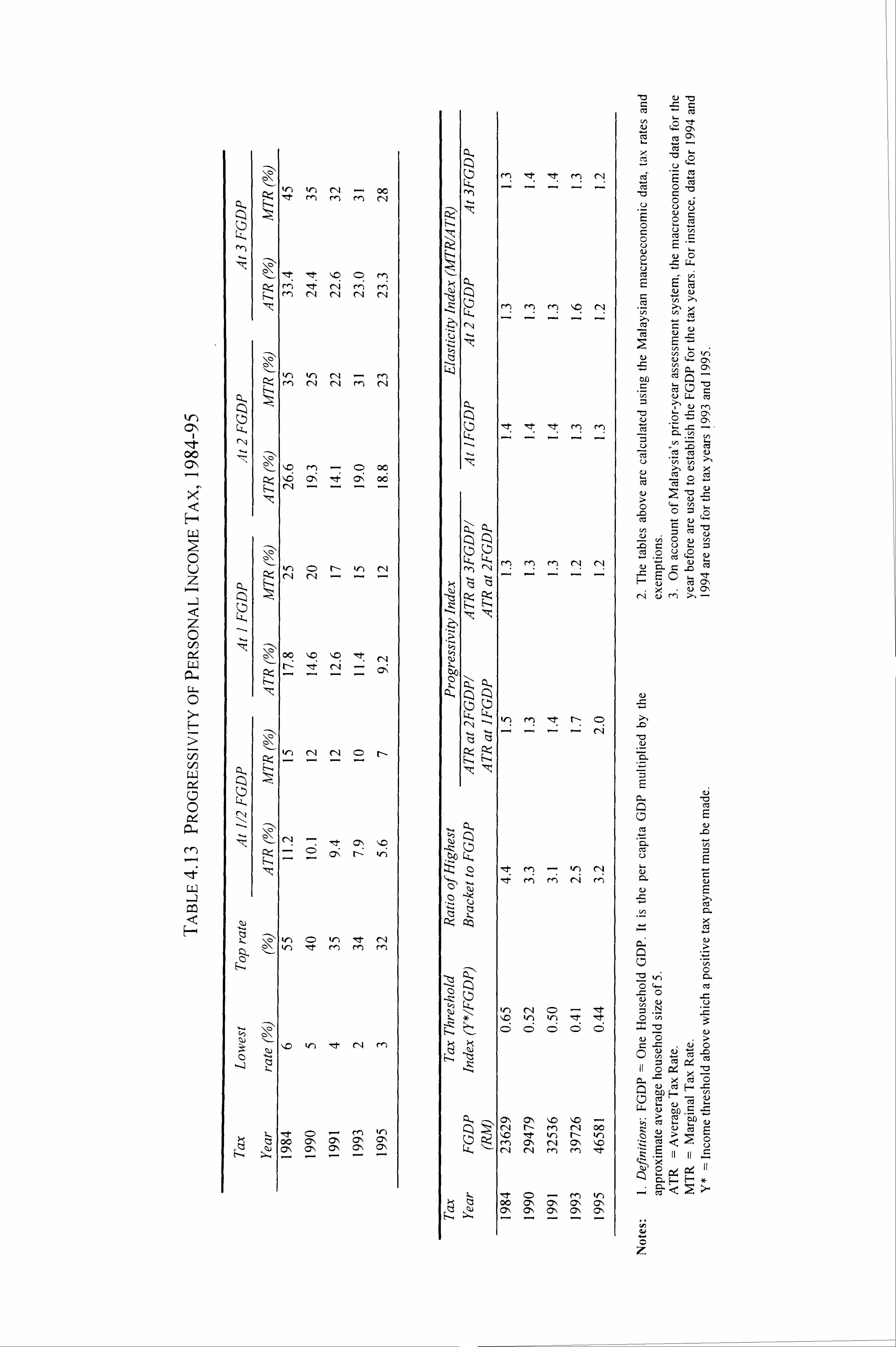
00

H

C

z

z 0 ctJ

0

> C/D cf

0

H

cLý CZ

N - N

ýz-, ýe ýe �0 CD rn Ctý rl) e rq rf) rn

Q �0 c> -eý c, oo

C) t-- W-ý rq

CIA

, I- C, 4

ýt ýü "Z ke) ý2t C, 1 rn

r. ý oo *e z c> -- - o', 12� ll', ý

I

I

rn rN

IZ,

Lz,

CL, ---,

fn 110 CIA

,ete rn rn

rrrrc

---

Nr

kn

C" C", I'D 1,0 - C14 r- en rl 00 Iýc "Ril V-1 kr)

cf) (0", C-4 "o

kr) 00 0ý 0*1 Cý cl, 01ý clý cl, 011, C7ý

73

CD 73 72 r_

CD

"c ýD 1C3

CD

-m

Z 0 c: C) k. =$ m

.2 cli 42 u

x-u Cý rý (U rn >, -

-0

75 r-

a. 6

"a

-0

al

kt*)

C) u (p -ýý -0

M

CHAP TER 4 STRUCTURE, 4ND TPEND OF THE TixSisTEm

One reason for this is that the rapid rise in average family GDP that brought many families into the taxable income brackets or the problem of 'bracket creep'.

Second, the personal relief schedule had changed very little since 1980 despite

the increase of around 40 percent in the price level between 1980-90. For instance, a working individual with four dependants and who earned RM12,900 in 1980 would not be paying any tax. However, if he was to earn the same amount of real income in Y/A

1984, he would fall into the 6 percent tax bracket. The same real income would bring

him into the 8 percent bracket in Y/A 1990 and the 10 percent bracket in Y/A 1991. In

other words, he would indeed be worse off since the rising nominal income would move him into successively higher tax brackets. However, the situation is reversed with the

latest tax rate revisions. The increase in personal relief and reduction of tax rates in the

nineties would bring him down the 8 percent bracket in Y/A 1993 and the 0 percent bracket in Y/A 1995.

There is also a substantial compression of marginal tax rates. The ratio of the

highest bracket to FGDP falls from 4.2 in 1984 to 3.2 in 1995. This implies that

individuals reach the highest tax bracket earlier in 1995 than a decade before. However,

this trend is also accompanied with falling marginal tax rates, including the highest tax

bracket, over time. This is shown by the declining marginal tax rates at each multiple of

FGDP in Table 4.13. Marginal tax rates fell between 12 to 17 percentage points for the

first three multiples of FGDP.

The Progressivity Index shows the effective progressivity between multiples of

FGDP. The progressivity for tax payers in the middle income and medium-high income

category had increased from 1.5 ten years before to 2.0 in 1995. By contrast the

progressivity index of those in the medium-high and high income category had remained

relatively unchanged. The Elasticity Index shows the relationship between marginal and

average tax rates. The index shows that the Malaysia's tax rates are structured such that

the elasticities remained fairly constant between 1.2-1.4 for the first three multiples of

average family income between Y/A 1984-1995.

Horizontal equity is violated when similar taxpayers are not treated in a like

fashion as a result of uneven enforcement of tax compliance across different classes of

103

CHAPTER 4 STRUCTURE, 4ND TREND OF THE TA, )CS)'STE. ýf

taxpayers and types of income. From the Household Income Survey 1989, the number of households that are estimated to pay taxes are between 1.2 and 1.3 million although about 1.0 million households are assessed for income tax, implying a participation rate of 78 percent to 85 percent. The majority of those who pay taxes are on employment rolls. However, there are under-reporting of income among those who are not on these rolls,

which suggests that there is uneven coverage of the personal income tax. It has yet to be

established whether different segments of society bear a disproportionately high or low

share of the burden.

3.1.2 Corporate Income Tax

Corporations are levied a flat tax rate on their undistributed profits. There is some

degree of integration between personal and corporation taxes, where dividends are taxed

once and individuals are allowed credit for taxes paid by the corporation on their behalf

Corporate taxation has long been an important source of government revenue. It

contributed about 25 percent of tax revenue in 1970, but its share dropped to around 20

percent from 1973 through 1991, before rising to above 26 percent in the early 1990s. To

increase govermnent revenue during economic recession in the mid-seventies, the

corporate and development tax rates were adjusted upwards from 45 percent to 50

percent in 1975. The 5 percent increase was because of the imposition of the excess

profit tax, which was abolished in Y/A 1988. The 50 percent tax rate was maintained for

a decade before the downward rate revisions, starting from Y/A 1986 to reach 30 percent

in Y/A 1995 (see Table 4.14). This process of lowering the corporate tax rate was to

bring it more in line with the taxes of neighbouring countries. 8 Despite the rate

adjustments, the contribution of corporate tax to the Malaysian government tax revenue

rose from 23 percent in 1986 to 28 percent in 1995. Clearly, the tax revenue accrued

from the rapid rise in business activities and corporate profits had more than

compensated for the revenue loss from the tax rate adjustments.

8 The corresponding corporate tax rates in the ASEAN countries are 27 percent for Singapore, 30 percent Z: 5 for Thailand, Brunei, and Indonesia, and 35 percent for the Philippines.

104

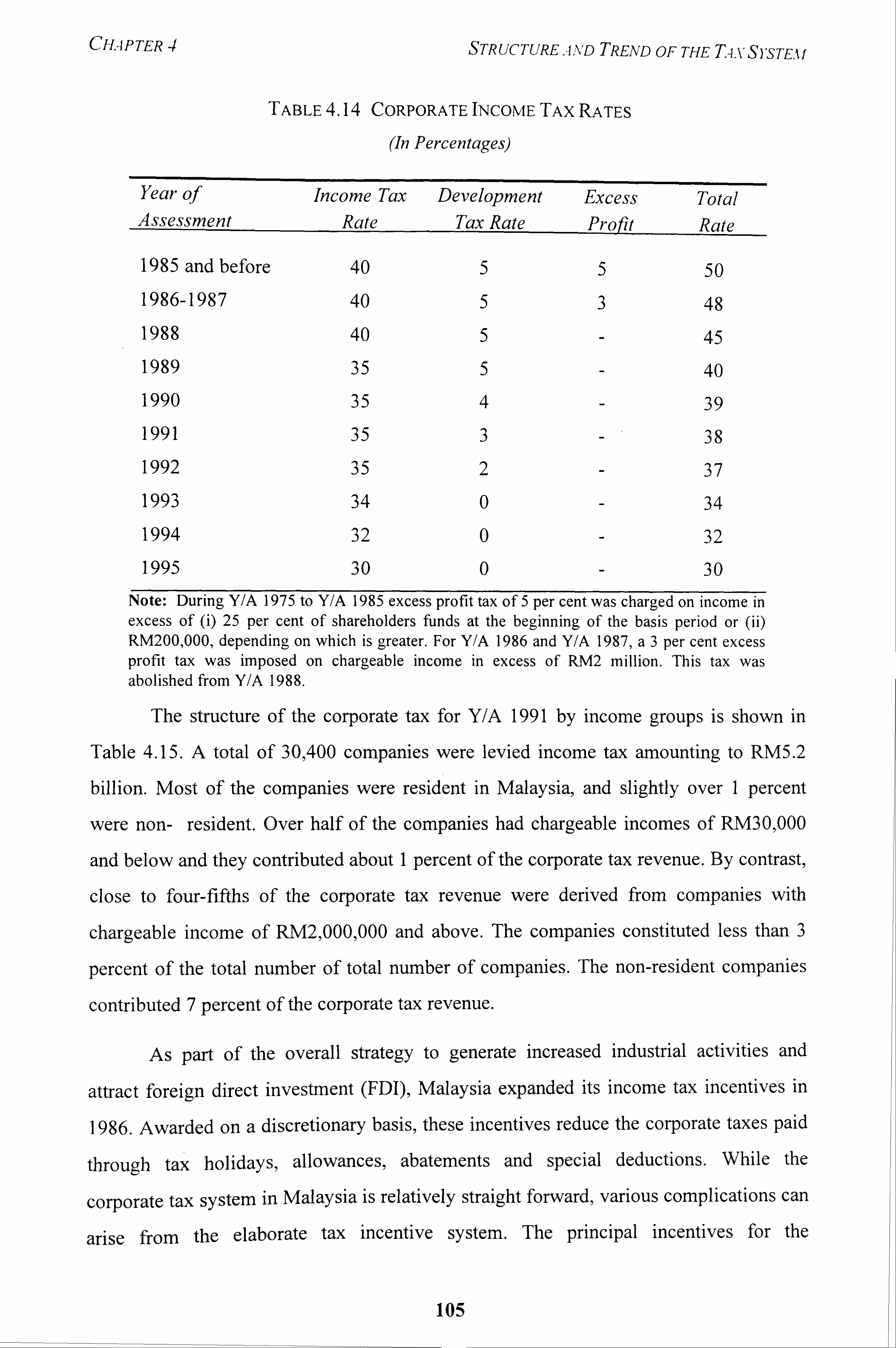
CHAPTER 4 STRUCTUREAA'D TREND OF THE T4xS), sTE. if

TABLE 4.14 CORPORATE INCOME TAX RATES

(In Percentages)

Year of Income Tax Development Excess Total Assessment Rate Tax Rate Profit Rate

1985 and before 40 5 5 50 1986-1987 40 5 3 48 1988 40 5 - 45 1989 35 5 - 40 1990 35 4 - 39 1991 35 3 - 38

1992 35 2 - 37

1993 34 0 34

1994 32 0 32

1995 30 0 30 Note: During Y/A 1975 to Y/A 1985 excess profit tax of 5 per cent was charged on income in excess of (i) 25 per cent of shareholders funds at the beginning of the basis period or (ii) RM200,000, depending on which is greater. For Y/A 1986 and Y/A 1987, a3 per cent excess profit tax was imposed on chargeable income in excess of RM2 million. This tax was abolished from Y/A 1988.

The structure of the corporate tax for Y/A 1991 by income groups is shown in

Table 4.15. A total of 30,400 companies were levied income tax amounting to RM5.2

billion. Most of the companies were resident in Malaysia, and slightly over I percent

were non- resident. Over half of the companies had chargeable incomes of RM30,000

and below and they contributed about I percent of the corporate tax revenue. By contrast,

close to four-fifths of the corporate tax revenue were derived from companies with

chargeable income of RM2,000,000 and above. The companies constituted less than 3

percent of the total number of total number of companies. The non-resident companies

contributed 7 percent of the corporate tax revenue.

As part of the overall strategy to generate increased industrial activities and

attract foreign direct investment (FDI), Malaysia expanded its income tax incentives in

1986. Awarded on a discretionary basis, these incentives reduce the corporate taxes paid

through tax holidays, allowances, abatements and special deductions. While the

corporate tax system in Malaysia is relatively straight forward, various complications can

arise from the elaborate tax incentive system. The principal incentives for the

105

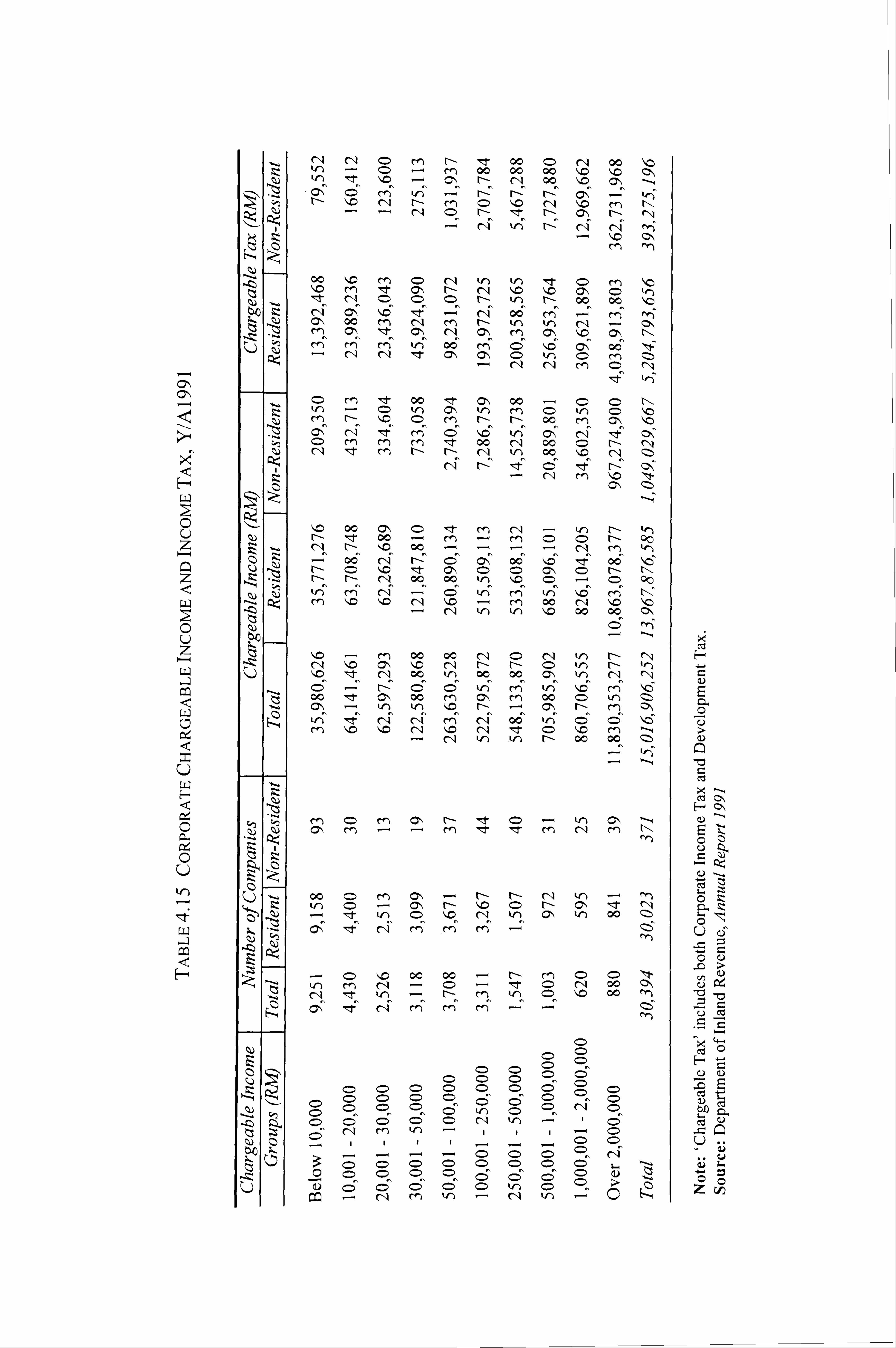
v --- 4 (os\

cq C-11 C) r-- Ni- 00 C) cc ýo kn c> 00 00 00 11C ýlc r-- ('A 00

r- \ýc r-- rn Cý "o rq ý, c rn r-ý

00 \C m C) kn Ln :t (:: ) \C) ýc rfl) Nt 01-1 r- r1l 110 110 c7lý tn

' C) C) C) rl- V-) tl- 00 00 \C)

clý Cý \6 llý' --ý 06 r-ý ffý llý a\ 00 m m kn V-) - CN m Cý -zt Cý, C-4 Cý m cr, ,c Cý (, - clý clý rlý krý oe rlý Cý 116 Cý' oe 11! 1ý

Iýt 00 c-) 00 (:: > kn Cý kf) M (:: ) V) (:: ) \0 r-- 110 C) m t-- r-- COO m C\ \0 Cý r-ý clý Cý Ile krý Cý' C) m m Izi- cq 00

rl- 00 ý10 cli

'-. c 00 Cý C) Iýt m C'4 - V) r- kr) r- 'tj- 00 - M -4 m r- 00

t-- 00 -ý - ý m krll

06 r--zl Cý Cý' oe oe \CT r- 6 "d -, t (7N C> (=> Cý\ (=) C-- t, - t-- r-- C14 00 00 tn "C (:: ) - 00 trý clý Cýl Cý Vý r-ý Vý Ile C-ý t-ý - M 00 " "C \0

kn tn l%C cc 00 0\

, ýc - m 00 00 (=) kn r- N "D a, \c r- t-- Cl r- te)

Cý 00 m (0ý, m 00 kn

, kn kn ý, o r--

' c-, m

trý 14 clý C4 rlý cllý 06 krý Cý Cý \6 -Q m ý, c ,c (-, I ý, c " . Zt ý= Ic C") --I >

os

CC C: ) M k1r) (=) Cý t-- ý, c Cý r- C', ý Iýt N a. z C> ,, c (, \I Cý 00 0 C ý .

-0 > ý, c cc cc C> ', I-

O a)

04 C, 4 ý C: ) OC N CA Tt kn - C-- rn In C: ) "D oc ('n 'a ýc

- r .- r.

0-4

C) C)

c, C) Cý3 C> bO

kn C) C) u

c)

Z

CHAP TER 4 STRUCTURE, qAD TREND OF THE T4xS)'STE. vf

manufacturing sector are contained in the Promotion of Investments Act (PIA), 1986 and the Income Tax Act, 1967. Among some of the most important forms of tax incentives

available are the following: 9

(a) Pioneer Status for investments in agriculture, industrial and hotel;

(b) Investment Tax Allowance for companies producing 'promoted products';

(c) Industrial Adjustment Allowance which allow specific manufacturing

companies in textile, wood, motor cars, shipbuilding, oil palm and bar and rod

rollings;

(d) Abatements to companies which are not claiming the ITA or pioneer status;

(e) Reinvestment Allowance for manufacturing companies which incur

qualifying capital expenditure for the purpose of an approved expansion; and

(f) Specific export and other incentives.

One can reasonably raise questions on the extent to which Malaysia's tax

incentives have helped either to increase inward FDI or give domestic firms an edge in

world trade competition. It is, however, difficult to attribute or measure the contribution

of particular incentives to increase foreign direct investment. Most developing countries

prefer to have high nominal rates of corporation tax and then grant exemptions

selectively which erode the marginal effective tax rate. In surveying tax incentives across

twenty-eight developing countries, Shah and Toye (1978) note that as opposed to theory,

tax holidays and tax credits, subsidies to earnings and subsidies to investment are not

alternatives , in practice. Firms could be allowed to opt and benefit under one scheme or

the other, according to which would provide the greater subsidy. To gain maximum

benefit from the tax and incentive schemes, firms would take advantage of their tax

holidays until their expiry, and then enjoy the different kinds of depreciation allowance

and tax credit available. The most popular incentive scheme is the tax holiday which

provides the largest element of subsidy to firms which earn profits (Heller and Kauffman,

9 The full range of investments available are listed and described in the 'Investors' Guide' of the

Economic Report.

107

CHAPTER 4 STRUCTURE AND TREND OF THE T4, vS)sm. ýf

1963: 85; Usher, 1977,131-32). The basic tax holiday is extended and supplemented by other types of tax concessions.

It is important to consider the interaction of incentives since some incentives can render others ineffective. In examining the incremental effects of incentives, Pellechio, Sicat and Dunn (I 987a) found that five-year tax holiday and import tax exemption

eliminated the beneficial effect of an investment deduction. When the benefits of tax incentives occur at the same time some of them become redundant. The problem of indiscriminate granting of tax incentives is that they erode the tax base and may not promote the desired mix of investments. For policy making, it is important to know

about the exact impact of tax incentives on the effective tax rates faced by investors, on the composition of overall investment, and on the substitution of the factors of

production. The lack of knowledge in these areas, as is often the case, can lead to the

creation of an excessive number of incentive instruments.

In their study on the taxation of investment in East Asian countries, Pellechio,

Sicat and Dunn (1987a) show that the statutory (or nominal) corporate income tax rate

gives a misleading picture of the true effective tax rate, which is modified by significant deductions allowed for depreciation, investment allowances, and income abatement. The

tax rate is further reduced by a five-year tax holiday applicable to companies with

pioneer status. In addition, favourable treatment of capital gains and an offset against

personal income taxes of corporate taxes paid on dividend receipts act to lower the tax

burden. One way of assessing the impact of corporate taxes is through the use of a

simulation model developed in the World Bank. 10 By using purely hypothetical data

based on actual parameters of the tax system and the average capital composition of

investment projects, this model computes a cash-flow stream before taxes and after taxes.

Allowances are made for depreciation, interest deductions, loss offsets, capital gains')

personal income tax credits against dividend payouts and other features. The percentage

10 See A. Pellechio, G. Sicat and D. Dunn, 'Taxation of Investment in East Asian Countries, ' DRD Discussion Paper No. 26 1, World Bank, March 1987.

108

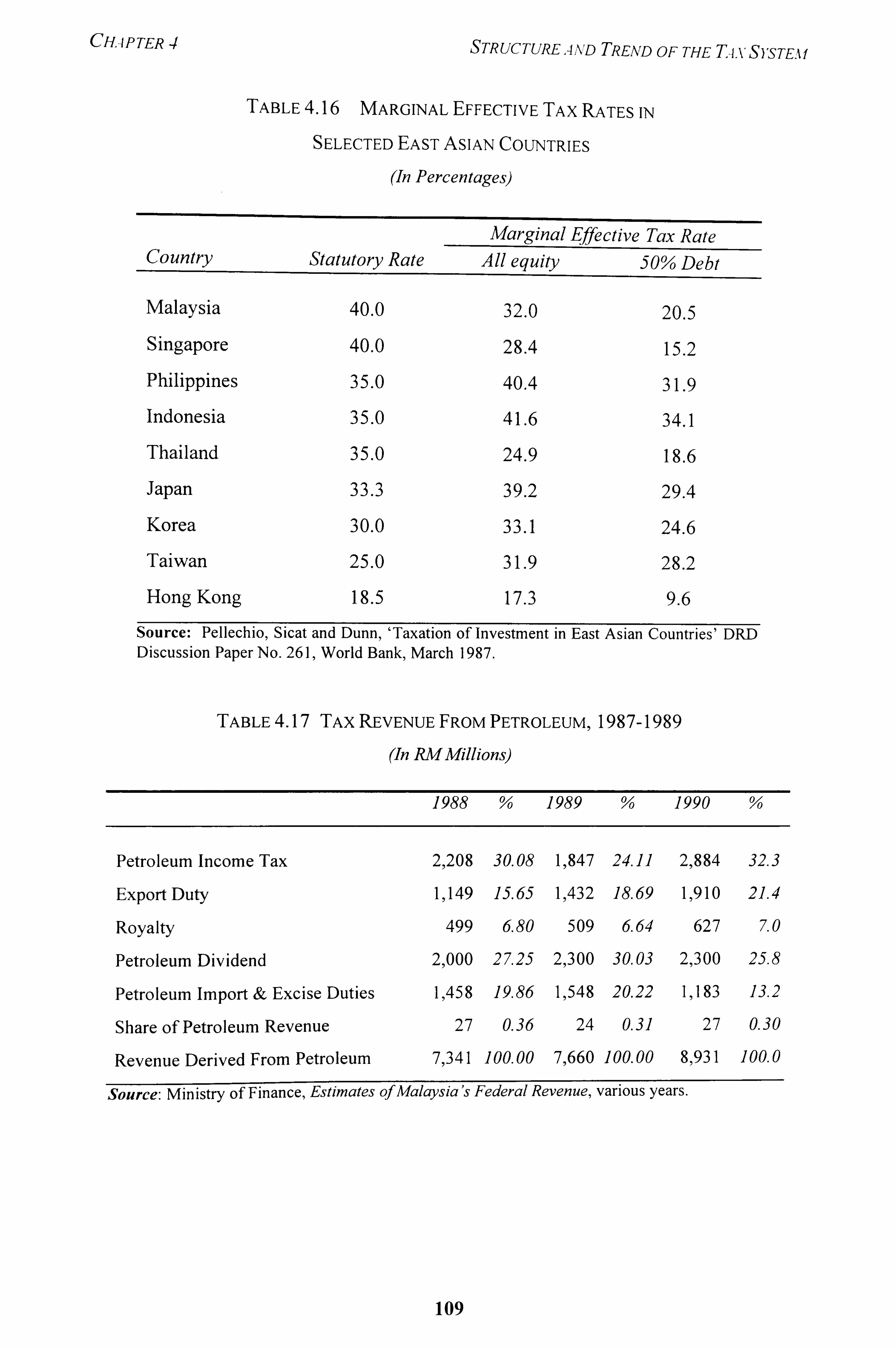
CHAPTER 4 STRUCTURE. 4A, D TREArD OF THE Ti. vS)'STEm

TABLE 4.16 MARGINAL EFFECTIVE TAx RATES IN

SELECTED EAST ASIAN COUNTRIES

(In Percentages)

Marginal jýffective Tax Rate Country Statutory Rate All equity 50% Debt

Malaysia 40.0 32.0 20.5

Singapore 40.0 28.4 15.2

Philippines 35.0 40.4 31.9

Indonesia 35.0 41.6 34.1

Thailand 35.0 24.9 18.6

Japan 33.3 39.2 29.4

Korea 30.0 33.1 24.6

Taiwan 25.0 31.9 28.2

Hong Kong 18.5 17.3 9.6

Source: Pellechio, Sicat and Dunn, 'Taxation of Investment in East Asian Countries' DRD Discussion Paper No. 26 1, World Bank, March 1987.

TABLE 4.17 TAx REVENUE FROM PETROLEUM, 1987-1989

(In RM Millions)

1988 % 1989 % 1990 %

Petroleum Income Tax 2ý208 30.08 19847 24.11 29884 32.3

Export Duty 1ý149 15.65 11432 18.69 1,910 21.4

Royalty 499 6.80 509 6.64 627 7.0

Petroleum Dividend 21000 27.25 21300 30.03 2,300 25.8

Petroleum Import & Excise Duties 1,458 19.86 1 ý548 20.22 IJ83 13.2

Share of Petroleum Revenue 27 0.36 24 0.31 27 0.30

Revenue Derived From Petroleum 7,341 100.00 7,660 100.00 8ý931 100.0

Source: Ministry of Finance, Estimates of Malaysia's Federal Revenue, various years.

109

CHAP TER 4 STRUCTUREAAD TREAD OF THE TtVS), sTEvf

difference in the rate of return generated by the before-tax and after-tax streams is designated the marginal effective tax rate (METR).

The simulation results of the METR of Malaysia and the other Asian countries are

shown in Table 4.16. Malaysia's METR IS significantly lower than its statutory rates,

especially if debt financing is used. These calculations only consider the minimum

allowances accorded to companies. If other deductions and exemptions are included, the

rate can decline further. For instance, a pioneer company with a 5-year exemption using 50 percent debt financing would face a METR of only 15 percent. If losses from a project

can be used to offset income earned elsewhere in the corporation, then the METR falls to

10 percent. If the pioneer status is extended from 5 to 10 years, the METR falls to a

minimal of 4 percent. On this basis, one can conclude that Malaysia's effective tax rate is

low enough not to discourage new investments, a statement that is supported by Tahir

(1984).

For many new companies that qualify for pioneer status, the tax burden has been

so much reduced by major incentives that they could afford to overlook minor credits and

deductions, such as the Labour Utilisation Relief (now abolished) and the Double

Deduction for Training. Besides the pioneer status, companies can also opt for the

Investment Tax Allowance (ITA), which tends to be favoured by large, capital -intensive

projects, or the Reinvestment Allowances and accelerated depreciation allowances under

the provisions of the Income Tax Act. The low effective tax rate on capital as the result of

the incentives may have contributed to an erosion of the tax base as well as the

unintended consequence of biasing projects towards more capital-intensive techniques

(World Bank, 1989). A tax structure with fewer exemptions would permit more effective,

selective tax incentives than the present system. II In addition, the lowering of the

statutory tax rate from 45 percent to 30 percent would need to be accompanied with the

I One of the most dramatic reform of investment incentives in the eighties occurred in Indonesia. Before 1983 its tax structure was inordinately complex as a result of hundreds of ad hoc amendments such that

they were incomprehensible to taxpayers and tax collectors alike. The massive range of contradictory

investment incentives resulted in a complicated system that was ineffective in raising revenue. In

reforming its taxes, Indonesia abolished all special tax incentives, including tax holidays, investment

allowances, and accelerated depreciation. This reform resulted in administrative simplicity, transparency, and minimum distortion of economic behaviour. The expected revenue gains arising from

the elimination of incentives allowed the tax rate to be reduced (World Bank, 1988; Gillis, 1989).

110

CHAPTER 4 STRUCTUREAND TREND OF THE T4xSiSTE. w

removal of exemptions and investment allowances, without which the METR would fall below zero (World Bank, 1989: 7 1).

3.1.3 Petroleum Income Tax

Oil production in Malaysia started in 1911, but only grew in importance in the

early 1970s. Since the mid-seventies, the contribution of petroleum production to

government finance grew in importance. The share of petroleum income tax to total tax

revenue rose from 7 percent in 1975 to 21 percent in 1986, before declining to 5 percent

in 1995. Besides petroleum income tax, there are other sources of tax revenue derived

from petroleum, such as export duty, petroleum royalty and dividend, as well as import

and excise duties. In 1990 taxes and duties on petroleum contributed RM8.9 billion to Federal Government revenue (Table 4.17). Petroleum income tax accounted for 9.9

percent of government revenue, followed by petroleum dividend (7.9 percent), the export duty on petroleum (6.6 percent) and the petroleum royalty (2.2 percent).

Petroleum exploitation in the seventies influenced developments in the Malaysian

economy in a number of ways. Firstly, the share of the mining sector to GDP in 1990 is

far more important than anticipated in the Outline Perspective Plan, with the petroleum

sector emerging as the main contributor to the sector. The share of petroleum to the

mining sector increased from 16.5 percent in 1970 to 82.6 percent in 1990 export

commodity in the early 1980s, although its position and export value deteriorate relative

to palm oil exports in the early 1990s. Thirdly, the buoyant petroleum prices in the late

seventies and early eighties provided the government with revenue to finance ambitious

public sector programmes. However, the sudden fall in oil prices in 1986 caused a decline

in federal revenue and a cutback in public expenditure, which accentuated the recession

in the mid-eighties.

Malaysia abandoned the concessions system in favour of a system of production-

sharing contracts with foreign oil companies as specified in the Petroleum Development

Act 1974. Petronas, which was established under this Act, is vested the ownership of all

petroleum resources as well as the exclusive rights for exploration and production. The

production- sharing contracts specify the details with regard to the sharing of risks,

profits, and control over the different phases of the project: exploration, development and

ill

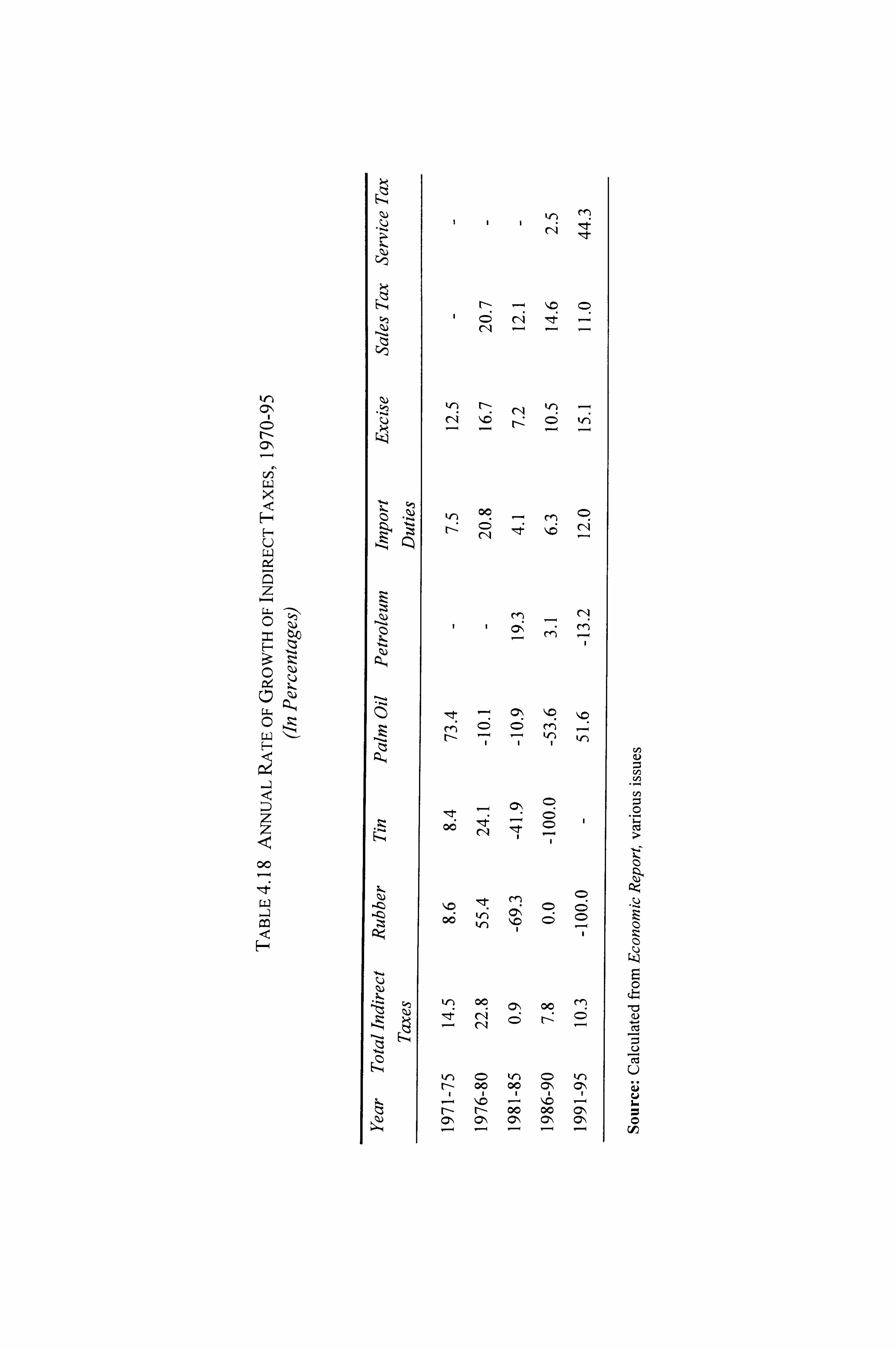
k, r)

LLI

ý4 Z,

0Z

oc

ýi 1 1 1

1,0 CD

rq

;Z c"i 1 1 0,1 rn

Z.,

CD CD

le CD 0

;Z c06 CD e

GoD In CD

-a

CD tri CD

0-, C> ollý 0*ý C> 0 lý -4 ---l cn

"

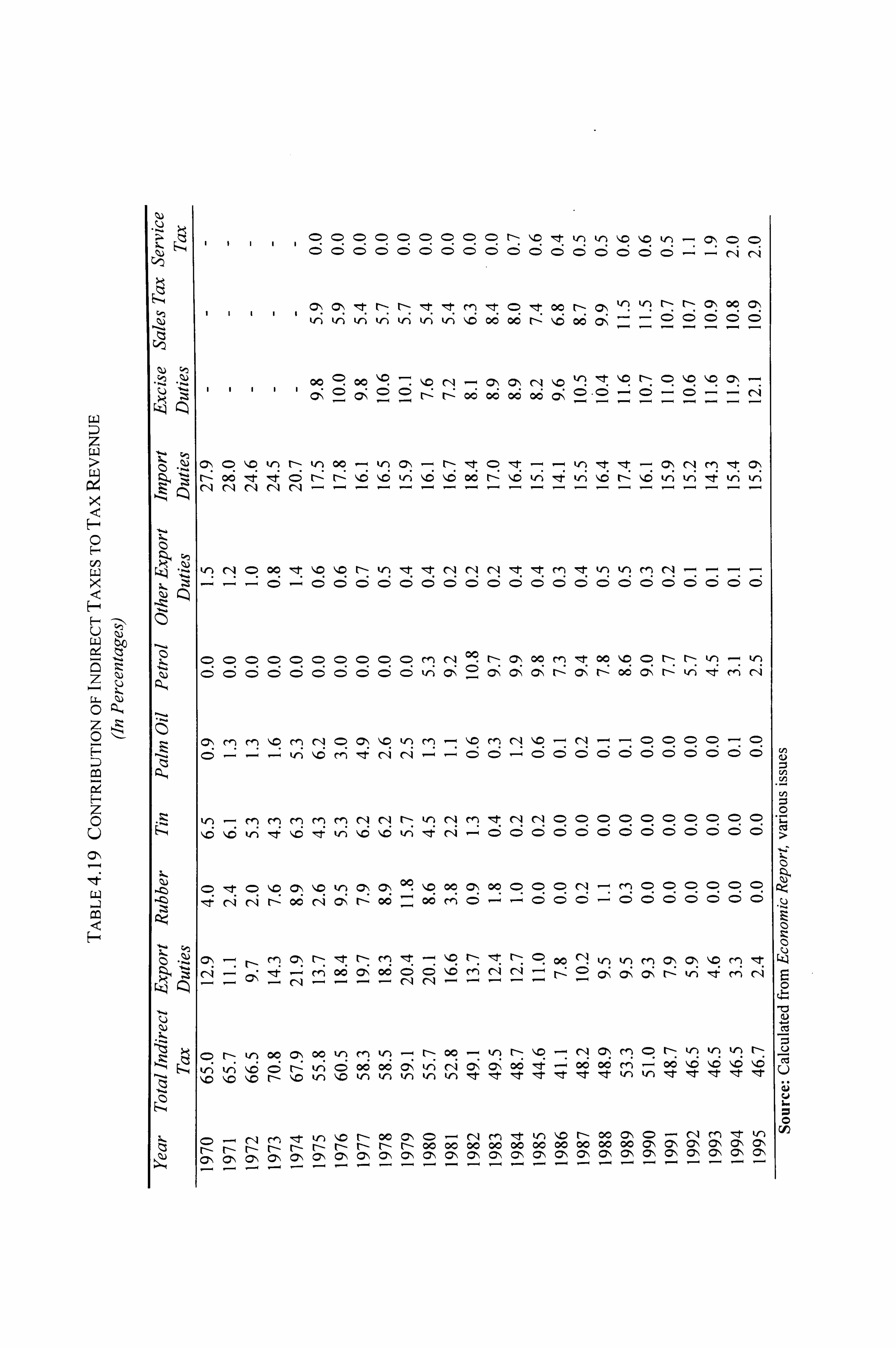
1--

all

LLJ

tn ýA)

ý"s Ln

%)

>-" ;Z ý4 cý

;3

-Z

cýI

,Z cs

;Z

c)

FF,

<Z c> cý c> ID c> CD CD Z 1-- �c, e f) 'rý -0 �0 v-) - c, CD c> CD CD (= CD (= CD CD CD CD CD CD CD CD c> CD CD CD -- C-A C-11

v' c, e r-- r- ýe �t rn -e c> -e oo r- v' n Irl ý, - ý, - Cý 00 C, CD CD CD CD CD kri krý o6 a', -

00 ý:: > oo �ýo -: 'z rq - c, c, ci �, Irl ýc ý, ý c> �0 ,0 cý, - el <Z el C> C> r- r- 00 00 Cd 00 c" C> - (=> -ý CD -- ("A

Cý C> I'D r- tn 00 (01ý, tl- C-, r-- 00 -4 4 C, r- r-- ýo ýo kn "o "o 00 r- "o "C; krý CII CA """- -ý ýýý -ý - --4 ý- -ý-----4ý--ý

tn -: t -zl- C'4 "" 'Zl- "t m "t tn kn m"ýý-- 66(:: ) 6 (6 (=) 6 c) C5 66 c) c) c,

c> CD C) c) c) c) 00 00 00 ýD C) r- r- c, (: 5 c, 6 (: 5 (::, CD a,

Cý, c-, a, Cý r-: Cý r-: 00 Cý r-

cý rn rn 1,0 rn C, 1 C> Cý 1,0 v) rn - 1,0 rr) rt Iso - (--1 -- CD CD CD CD - CD c> cý -ý cý cý cý c3 c; cý c3 cý cý cý c>

tn -mmMmm"" r-- kn "M mt " CNI C) C> CD CD CD CD C> C) C> C)

C5 C> C5 6 16 C; C-5 6 16 C) cl 6

cý ýe CD ým c, �0 V-ý c> c, 00 �0 00 c, 00 CD CD CD C-q -- rn CD CD CD CD CD CD 1. e (9 rý r--: oo rý c> r- o6 Z oo cý CD -- cý c> CD ý cý (: D CD cý CD CD c>

I-- , I: r-ý frý It - Iýq r-ý 1ý1- 'ý :ý 00 C! Lr) kn m a, cý "D m "t cn 00 Cý 00 C) C: ) ,c V)

Cý 00 tr) m tr) - r- 00 r- %C kn

kr) kn ,cc, t-- kn (6 00 oc C', kn rq c" C-, 00 1 ý. 00 oc m- 00 110 110 116 110 ý "C

ý'c "C r-- ý'o kn ýo kn tn tn k-r) Lr) -t -t 'I- -t- 't- -1- -zt kn kn -zl- "t -t -: t -T

CD c> CD - c-q rn -e V-ý \%O r- 00 O, \ CD

r-, r- 00 00 00 00 00 00 00 00 00 00 C> c7, cý, 0-, 0-, C, Cý C\ c*ý, O, \ Cý C> V, C> C> Cý C> C> Cý Cý\ cý V', C> C> Cl\ c> cý

0

sz

0

I :z

.2 03 u

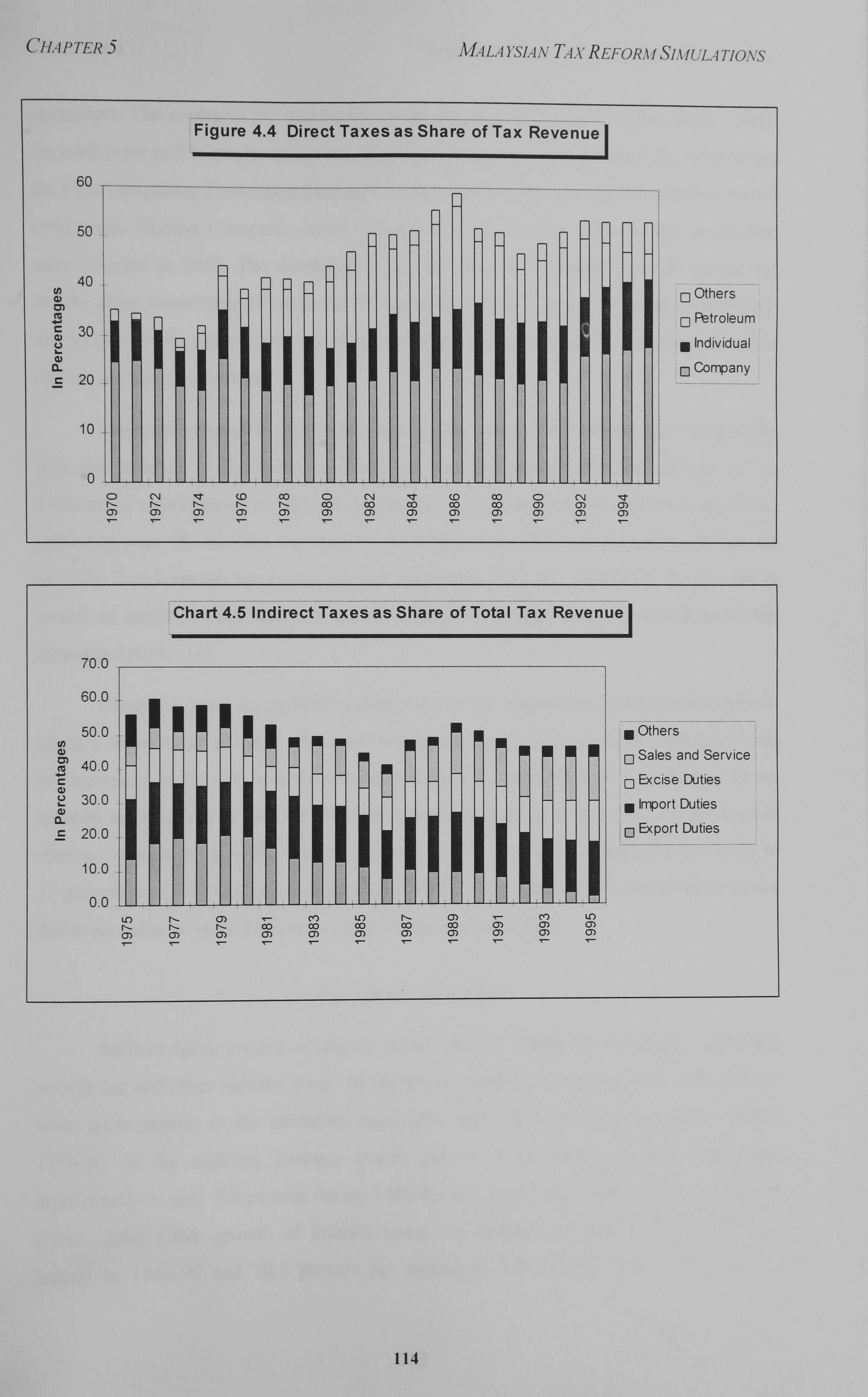
CHAPTER 5 MA LAYSIA N T4, v R EFORA I SIA IULA TIONS

Figure 4.4 Direct Taxes as Share of Tax Revenue

60

50

40

30

r- 20

10

Iýt III, Ll H1 ý -1

[-] I III IIII Ll 1- 11 1 11 11 L-1 1,1 Li 11 1 C) cli IT (C) OD C) CN lq- (D 00 C C\j 'IT

fl- r- r- r- 00 00 00 00 00 0) CF) C) cr) CY) o') CD 0) 0) CY) 0) (3) CV) CY)

Others

Petroleum

Individual

C] Cornpany

Chart 4.5 Indirect Taxes as Share of Total Tax Revenue

70.0

60.0

50.0 Others

4) tm E] Sales and Service

40.0 F: xcise Duties

P 30.0 --- ,0 Import Duties 4) a-

.S 20.0 i Export Duties

100 '

0. 0 U-) t1- rl- CF) L0 r- G) C0 Lr)

rl- r- co co 00 00 00 0') CY) CY) CF) CF) CY) CF) CF) a) 0) 0) 0) CF) CY)

114

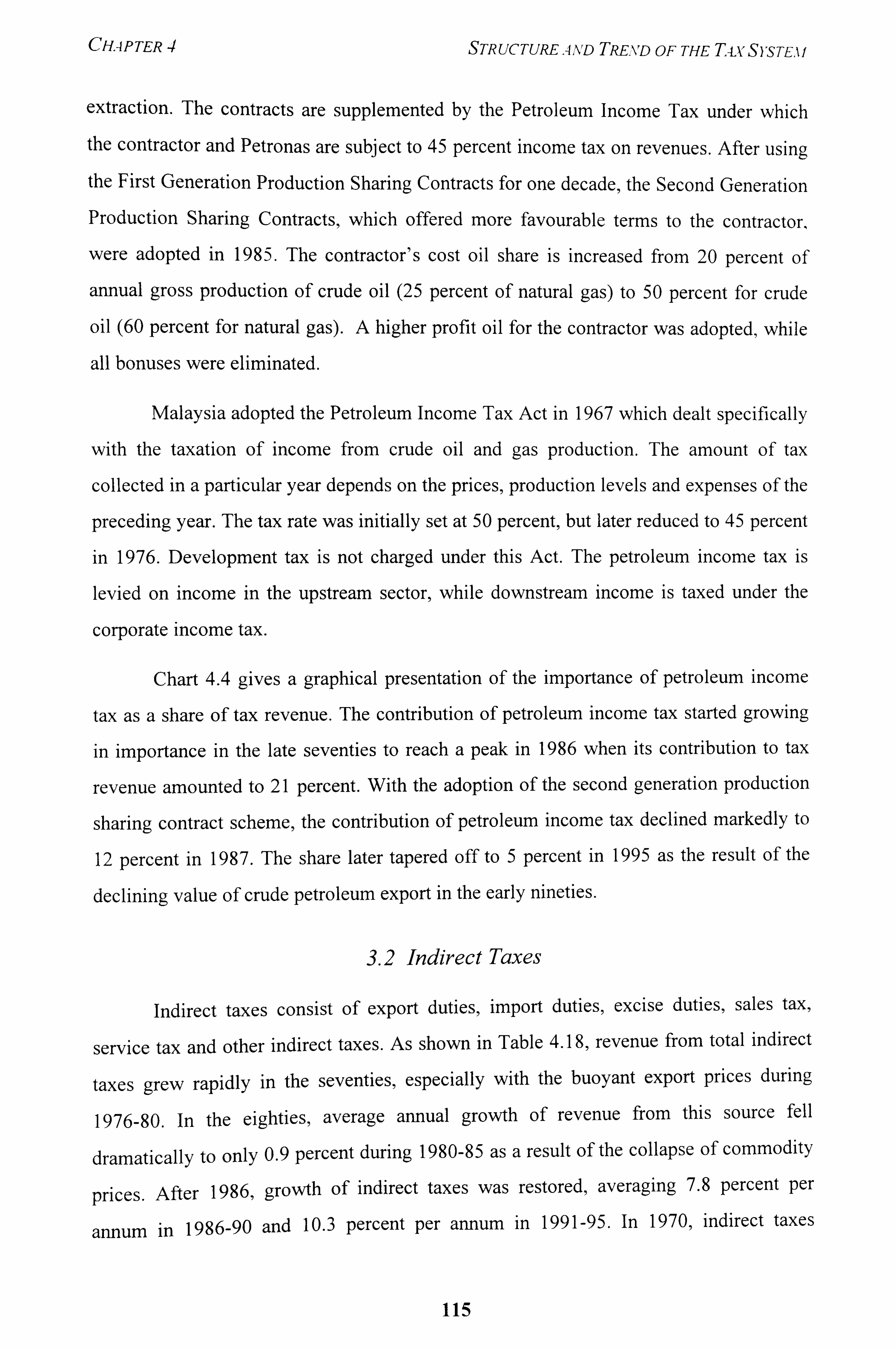
CHAPTER 4 STRUCTUREAND TRE. ND OF THE T-LvS)sTE, ýi

extraction. The contracts are supplemented by the Petroleum Income Tax under which the contractor and Petronas are subject to 45 percent income tax on revenues. After using

the First Generation Production Sharing Contracts for one decade, the Second Generation

Production Sharing Contracts, which offered more favourable terms to the contractor,

were adopted in 1985. The contractor's cost oil share is increased from 20 Percent of

annual gross production of crude oil (25 percent of natural gas) to 50 percent for crude

oil (60 percent for natural gas). A higher profit oil for the contractor was adopted, while

all bonuses were eliminated.

Malaysia adopted the Petroleum Income Tax Act in 1967 which dealt specifically

with the taxation of income from crude oil and gas production. The amount of tax

collected in a particular year depends on the prices, production levels and expenses of the

preceding year. The tax rate was initially set at 50 percent, but later reduced to 45 percent

in 1976. Development tax is not charged under this Act. The petroleum income tax is

levied on income in the upstream sector, while downstream income is taxed under the

corporate income tax.

Chart 4.4 gives a graphical presentation of the importance of petroleum income

tax as a share of tax revenue. The contribution of petroleum income tax started growing

in importance in the late seventies to reach a peak in 1986 when its contribution to tax

revenue amounted to 21 percent. With the adoption of the second generation production

sharing contract scheme, the contribution of petroleum income tax declined markedly to

12 percent in 1987. The share later tapered off to 5 percent in 1995 as the result of the

declining value of crude petroleum export in the early nineties.

3.2 Indirect Taxes

Indirect taxes consist of export duties, import duties, excise duties, sales tax,

service tax and other indirect taxes. As shown in Table 4.18, revenue from total indirect

taxes grew rapidly in the seventies, especially with the buoyant export prices during

1976-80. In the eighties, average annual growth of revenue from this source fell

dramatically to only 0.9 percent during 1980-85 as a result of the collapse of commodity

prices. After 1986, growth of indirect taxes was restored, averaging 7.8 percent per

annum in 1986-90 and 10.3 percent per annum in 1991-95. In 1970, indirect taxes

115

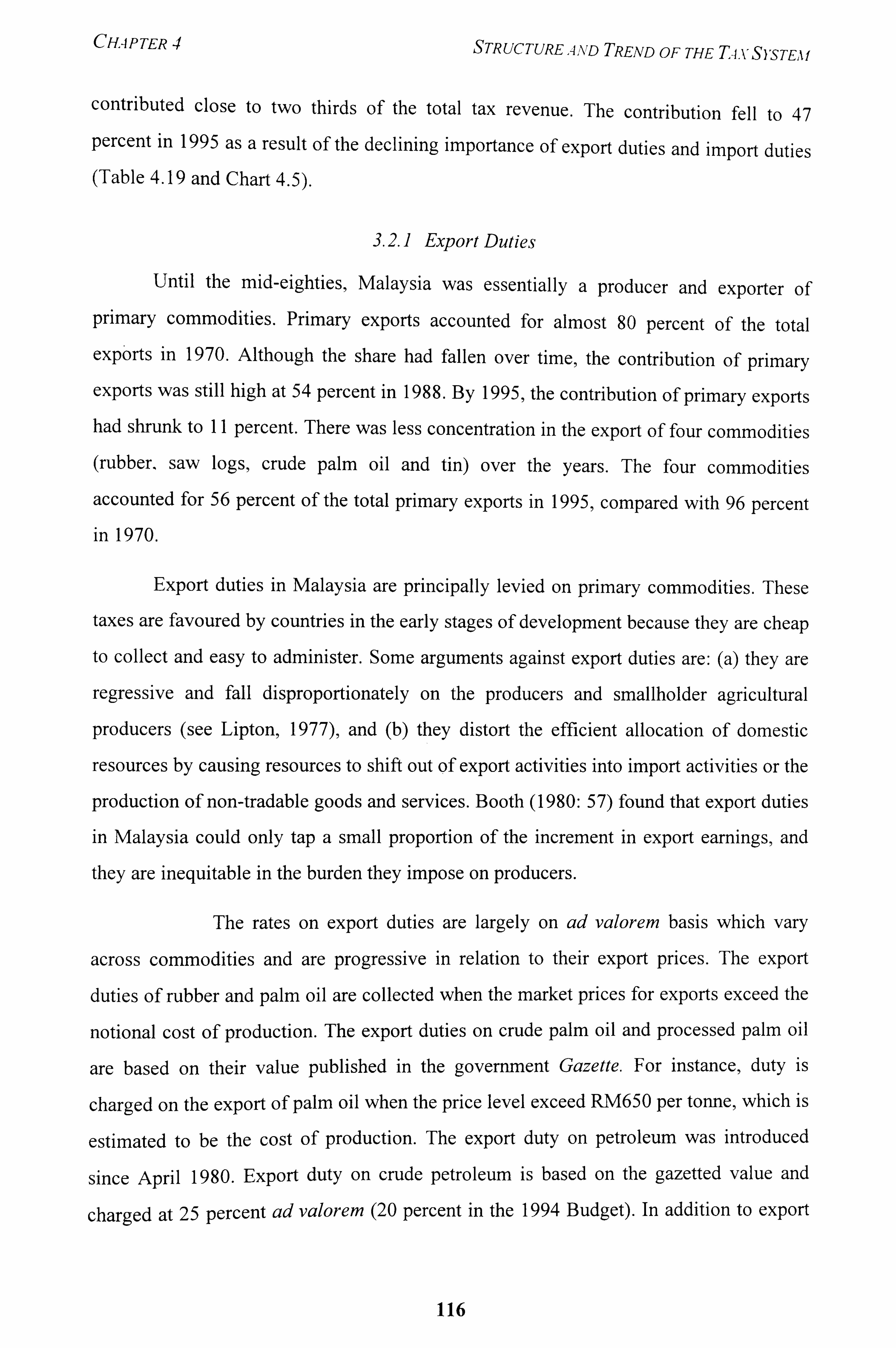
CHAPTER 4 STRUCTUREAAID TREND OF THE TIVSYSTEM

contributed close to two thirds of the total tax revenue. The contribution fell to 47 percent in 1995 as a result of the declining importance of export duties and import duties (Table 4.19 and Chart 4.5).

3.2.1 Export Duties

Until the mid-eighties, Malaysia was essentially a producer and exporter of primary commodities. Primary exports accounted for almost 80 percent of the total

exports in 1970. Although the share had fallen over time, the contribution of primary exports was still high at 54 percent in 1988. By 1995, the contribution of primary exports had shrunk to II percent. There was less concentration in the export of four commodities (rubber, saw logs, crude palm oil and tin) over the years. The four commodities

accounted for 56 percent of the total primary exports in 1995, compared with 96 percent in 1970.

Export duties in Malaysia are principally levied on primary commodities. These

taxes are favoured by countries in the early stages of development because they are cheap

to collect and easy to administer. Some arguments against export duties are: (a) they are

regressive and fall disproportionately on the producers and smallholder agricultural

producers (see Lipton, 1977), and (b) they distort the efficient allocation of domestic

resources by causing resources to shift out of export activities into import activities or the

production of non-tradable goods and services. Booth (1980: 57) found that export duties

in Malaysia could only tap a small proportion of the increment in export earnings, and

they are inequitable in the burden they impose on producers.

The rates on export duties are largely on ad valorem basis which vary

across commodities and are progressive in relation to their export prices. The export

duties of rubber and palm oil are collected when the market prices for exports exceed the

notional cost of production. The export duties on crude palm oil and processed palm oil

are based on their value published in the govermnent Gazette. For instance, duty is

charged on the export of palm oil when the price level exceed RM650 per tonne, which is

estimated to be the cost of production. The export duty on petroleum was introduced

since April 1980. Export duty on crude petroleum is based on the gazetted value and

charged at 25 percent ad valorem (20 percent in the 1994 Budget). In addition to export

116

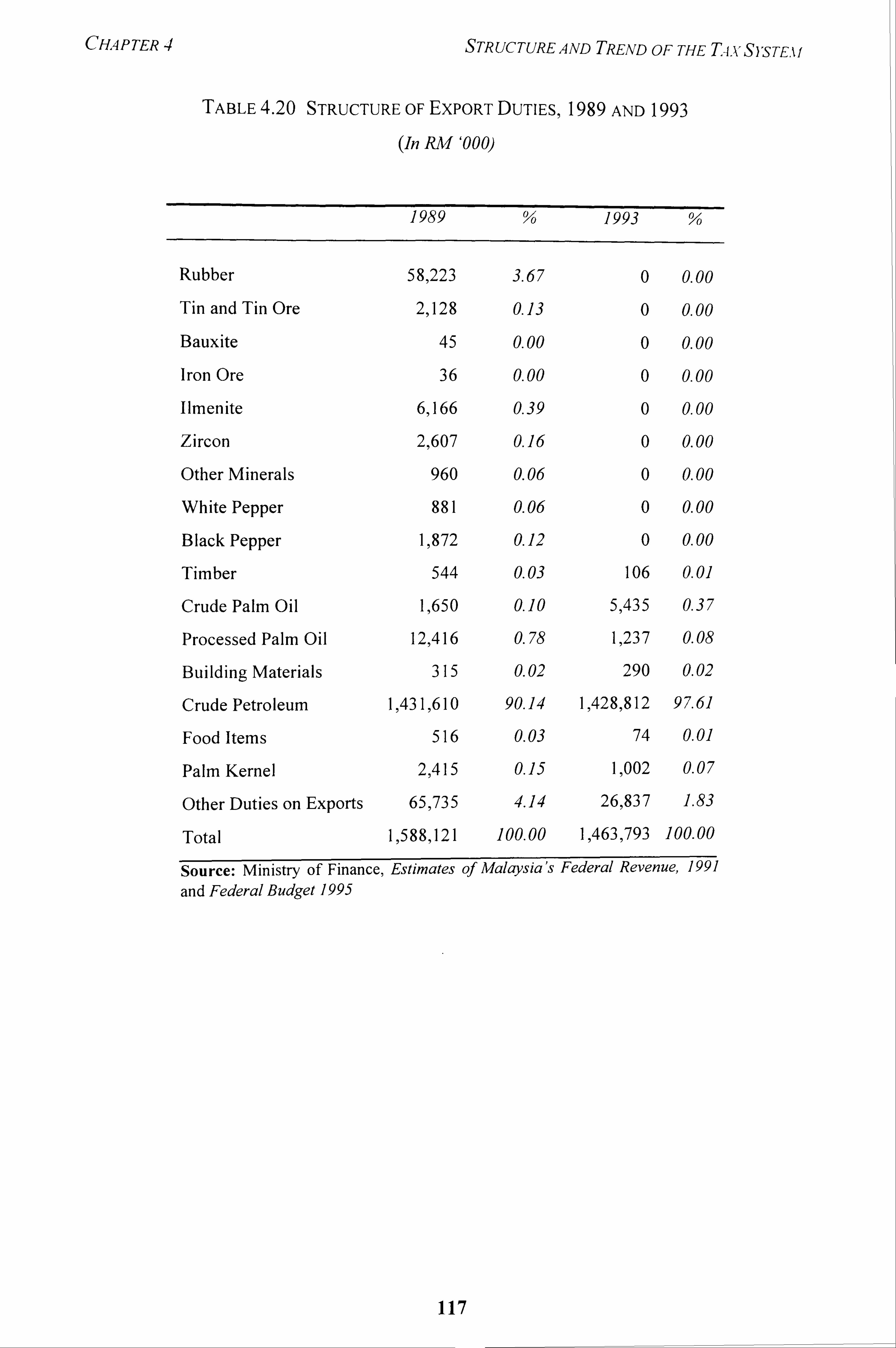
CHAPTER STRUCTURE AND TREND OF THE Tq. v S), sTE. k f

TABLE 4.20 STRUCTURE OF EXPORT DUTIES, 1989 AND 1993

(In RM '000)

1989 % 1993 %

Rubber 58,223 3.67 0 0.00

Tin and Tin Ore 21,128 0.13 0 0.00

Bauxite 45 0.00 0 0.00

Iron Ore 36 0.00 0 0.00

11menite 6,166 0.39 0 0.00

Zircon 2,607 0.16 0 0.00

Other Minerals 960 0.06 0 0.00

White Pepper 881 0.06 0 0.00

Black Pepper 15872 0.12 0 0.00

Timber 544 0.03 106 0.01

Crude Palm Oil 1,650 0.10 5,435 0.37

Processed Palm Oil 12ý416 0.78 1,237 0.08

Building Materials 315 0.02 290 0.02

Crude Petroleum 15431,610 90.14 1 ý428,812 97.61

Food Items 516 0.03 74 0.01

Palm Kernel 21415 0.15 11002 0.07

Other Duties on Exports 65,735 4.14 26ý837 1.83

Total 15588,121 100.00 15463,793 100-00

Source: Ministry of Finance, Estimates of Malaysia's Federal Revenue, 1991

and Federal Budget 1995

117

CHAPTER 4 STRUCTURE ý, IN, D TREND OF THE T4A'SYSTEA f

duties, rubber export is also levied research and replanting cess, while tin export is subject to research and development cess.

The changing composition of primary exports is reflected in the export duties collected. The tax revenue is highly cyclical, being determined by fluctuating world market prices. Export duties as a percentage of tax revenue peaked in 1974 (22 percent) as well as 1979-80 (20 percent), before declining throughout the eighties and into the nineties to reach 2 percent in 1995 (Table 4.19). The export duties for palm oil recorded negative growth rates during the mid-seventies, while the duties for rubber and tin started falling in the 1980s. The peaks corresponded with the buoyant prices of primary commodities (see Table 4.6).

In the 1991 Budget, the government abolished the export duties on rubber, pepper

and all minerals. A comparison of the structure of export duties for 1989 and 1993

wouldhighlight the effect of this abolition on the revenue accrued from this source (see

Table 4.20). Since 70 percent of rubber and all the pepper produced in the country are

grown by smallholders, the abolition of the export duties was expected to help improve

their income. As for tin, the revenue collected from export duty on tin has anyway been

insignificant since 1985. The fall in the collection of export duties from the traditional

commodities was only partially offset by petroleum export duty. But even then, the

collection of petroleum export duty started to decline after 1985. With less number of

goods subject to export duties, the amount of export duties collected has also fallen over

the years and is largely derived from petroleum export.

3.2.2 Im ort Duties

Since the colonial period, import duties were imposed to raise revenue, and in

some cases, to control the domestic supply of certain goods. In the 1960s, the strategy to

promote import substitution had led to a series of tariff increases in order to protect

domestic industry from foreign competition. The government had successively raised

tariffs on motor vehicles, consumer durables, tobacco products and alcoholic liquor. The

oil price hike in 1974 had pushed inflation into the double digits. To keep inflation down

and reduce the price burden on the poor, some 'essential commodities', such as sugar,

diesel oil, kerosene, wheat flour, condensed milk, fertilisers, and plywood were exempt

118

CH. AP TER 4 STR UCTURE. A ND TREND OF THE TIV SYSTEA f

from import duties (Ministry of Finance, Economic Report 1974175: 35; Asher and Booth, 1983: 88). The revenue foregone was approximately RM162 million or 12

percent of the estimated total import and excise duties in 1974.

Import duties are levied on a wide range of imports into Malaysia. The rates

generally vary from 0 to 100 percent, although CBU motorcars imports can be as high as 300 percent. Custom duty is mostly ad valorem although some specific taxes are charged

on a number of commodities. 12 The majority of imports are taxed between 10 and 35

percent. An import surcharge of 2 percent is levied on raw materials and some

machinery, while the rate of 5 percent is charged on other goods.

Malaysia has signed bilateral trade agreements with many countries 13

specifying the maximum rates of import duties and preference margins for particular

products. For ASEAN, the minimum Margin of Preference (MOP) is 25 percent. Various

exemptions are given when imports are used by government and public enterprises. In

addition, import duty exemptions are used in accordance with the industrial incentives

policies to promote certain types of investments and exports. The granting of tax

exemption on raw materials and machinery for the manufacturing sector depends on

whether the finished products are sold in the domestic market or exported. Imported raw

materials and components can qualify for full exemptions for the manufacturers who

produce finished products for export markets. A manufacturing company producing for

domestic market can qualify for import duty exemption as well if it complies with the

12 There generally are two main types of tariffs: (a) ad valorem duty which is levied as a fixed percentage of the value of the good; (b) specific duty which is levied as a fixed sum of money per physical unit of the good (Pass and Lowes, 1993). t: '

13 The countries that had signed trade agreements with Malaysia are Australia (1968), New Zealand (1961), United Arab Emirates (1962), South Korea (1962), Russia (1967), Bulgaria (1968), Rumania (1969), Yugoslavia (1969), Hungary (1970), Poland (1972), Czechoslovakia (1972), Indonesia (1973), Libya (1977), Turkey (1977), Bangladesh (1977), Democratic Republic of Korea (1979), German Democratic Republic (1980), Italy, Mali and ASEAN countries.

119

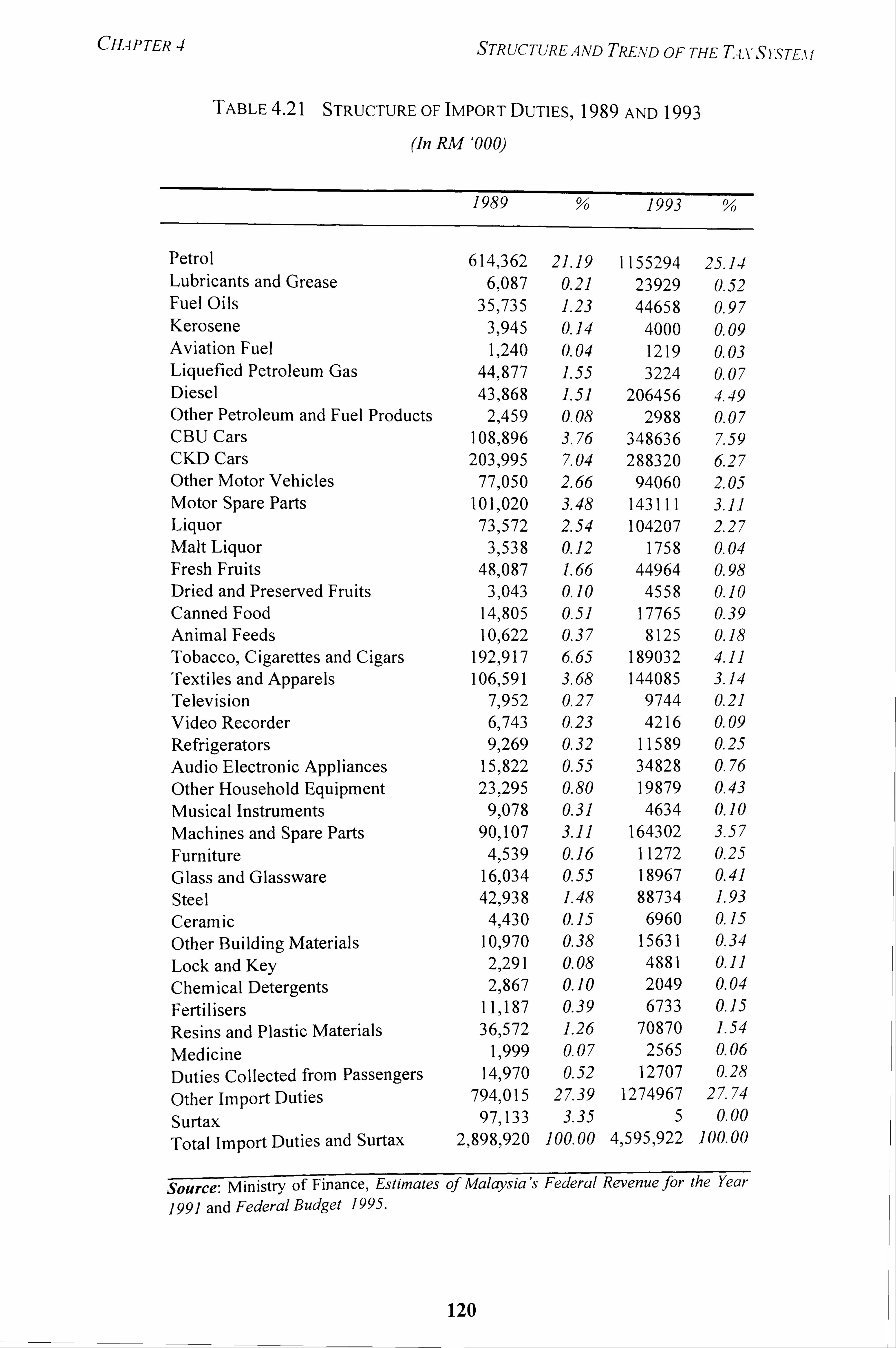
CH, APTER 4 STRUCTURE AND TPEATD OF THE T4XS)STE, k I

TABLE 4.21 STRUCTURE OF IMPORT DUTIES, 1989 AND 1993

(In RM '0 0 0)

1989 1993 %

Petrol 614,362 21.19 1155294 25.14 Lubricants and Grease 6,087 0.21 23929 0.52 Fuel Oils 35,735 1.23 44658 0.97 Kerosene 3,945 0.14 4000 0.09 Aviation Fuel 1,240 0.04 1219 0.03 Liquefied Petroleum Gas 44,877 1.55 3224 0.07 Diesel 43,868 1.51 206456 4.49 Other Petroleum and Fuel Products 2,459 0.08 2988 0.07 CBU Cars 108,896 3.76 348636 7.59 CKD Cars 203,995 7.04 288320 6.27 Other Motor Vehicles 775050 2.66 94060 2.05 Motor Spare Parts 101,020 3.48 143111 3.11 Liquor 73,572 2.54 104207 2.27 Malt Liquor 31538 0.12 1758 0.04 Fresh Fruits 48,087 1.66 44964 0.98 Dried and Preserved Fruits 3,043 0.10 4558 0.10 Canned Food 145805 0.51 17765 0.39 Animal Feeds 10,622 0.37 8125 0.18 Tobacco, Cigarettes and Cigars 192ý917 6.65 189032 4.11 Textiles and Apparels 106,591 3.68 144085 3.14 Television 7,952 0.27 9744 0.21 Video Recorder 6,743 0.23 4216 0.09 Refrigerators 9,269 0.32 11589 0.2-5 Audio Electronic Appliances 15,822 0.55 34828 0.76 Other Household Equipment 23,295 0.80 19879 0.43 Musical Instruments 95078 0.31 4634 0.10 Machines and Spare Parts 909107 3.11 164302 3.57 Furniture 4,539 0.16 11272 0.25 Glass and Glassware 16ý, 034 0.55 18967 0.41 Steel 42,938 1.48 88734 1.93 Ceramic 41430 0.15 6960 0.15 Other Building Materials 10,970 0.38 15631 0.34 Lock and Key 2,291 0.08 4881 0.11 Chemical Detergents 2!, 867 0.10 2049 0.04 Fertilisers 11ý187 0.39 6733 0.15 Resins and Plastic Materials 36,572 1.26 70870 1.54 Medicine 15999 0.07 2565 0.06 Duties Collected from Passengers 149970 0.52 12707 0.28

Other import Duties 794,015 27.39 1274967 27-74

Surtax 97,133 3.35 5 0.00

Total import Duties and Surtax 2,898,920 100.00 45595,922 100-00

Source: Ministry of Finance, Estimates of Malaysia's Federal Revenue for the Year

1991 and Federal Budget 1995.

120

CHAP TER 4 STRUCTURE, -i, ND TREArD OF THE TAXS)STEAf

equity condition of the New Economic Policy as stipulated in the manufacturing licence 14

. Exemptions will only be considered for raw materials and components that are not available locally.

During the last twenty five years, import duties have grown by almost elevenfold, from RM557 million in 1970 to RM6.0 billion 1995, and contribute between 3-4 percent of GDP to government revenue. The contribution of import duties to tax revenue has been fairly consistent since 1975 despite the reduction in import duties since the mid- 1980s. In the 1986 Budget the import duty on certain equipment used by fisheries and

agriculture was abolished, while import duty on a variety of raw materials were reduced to a uniform rate of 2 percent. The structure of imported duties for 1989 and 1993 is

shown in Table 4.21. The largest items are petroleum products and motor vehicles.

In the 1989 Budget, tariff protection for infant industries was reviewed, while import

duties for consumer products were reduced between 20-87 percent. In the 1990 Budget

the import duties and excise duties of food items, inputs for the agriculture sector and

household items were reduced to moderate price increases. The government abolished

import duties on rubber, tin and pepper in the 1991 Budget in order to encourage the free

flow of primary commodities into Malaysia. This measure was aimed at developing

Malaysia into the region's main centre for processing and manufacturing of agro-based

products and enhance the growth of the Kuala Lumpur Commodity Exchange. In the

later budgets, the government continued to reduce or abolish import taxes for 600 items

in the 1993 Budget, 500 items in the 1994 Budget, and over 26,000 items in the 1995

Budget.

3.2.3 Excise Duties

Excise duties are the oldest form of indirect taxes in Malaysia. They are levied on

imports as well as locally manufactured goods. The tax base for excise duties Malaysia

was extended in 1968, but this did not have a significant impact on revenue until an

excise tax on motor vehicles was introduced in 1970. In 1982 budget the government

abolished excises on some products, such as gas stoves, fans, electric irons, ovens, and

14 This is in relation to equity participation, management and employment structure.

121

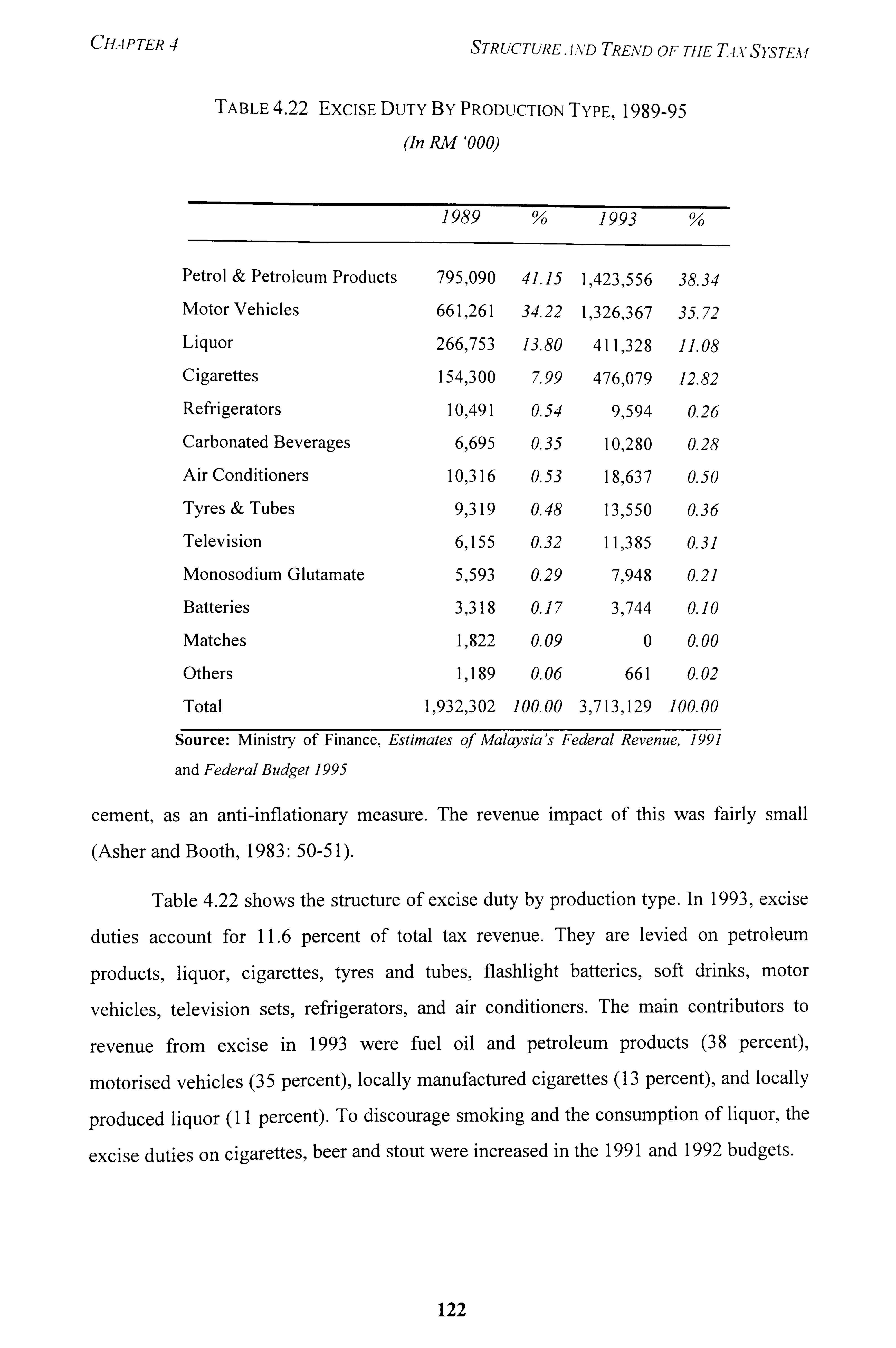
CHAP TER 4 STRUCTURE. -ivD TREND OF THE T4A'SYSTEAf

TABLE 4.22 ExciSE DUTY By PRODUCTION TYPE, 1989-95

(In RM '0 0 0)

1989 % 1993 %

Petrol & Petroleum Products

Motor Vehicles

Liquor

Cigarettes

Refrigerators

Carbonated Beverages

Air Conditioners

Tyres & Tubes

Television

Monosodium Glutamate

Batteries

Matches

Others

Total

795,090 41.15 1ý423,556 38.34

6615261 34.22 1,326,367 35.72

266ý753 13.80 411,328 11.08

154,300 7.99 476,079 12.82

10,491 0.54 9,594 0.26

6,695 0.35 10,280 0.28

10,316 0.53 18,637 0.50

9,319 0.48 13,550 0.36

6,155 0.32 11,385 0.31

59593 0.29 7,948 0.21

3,318 0.17 3,744 0.10

1,822 0.09 0 0.00

1,189 0.06 661 0.02

1ý932,302 100.00 31713,129 100-00

Source: Ministry of Finance, Estimates of Malaysia's Federal Revenue, 1991

and Federal Budget 1995

cement, as an anti-inflationary measure. The revenue impact of this was fairly small

(Asher and Booth, 1983: 50-5 1).

Table 4.22 shows the structure of excise duty by production type. In 1993, excise

duties account for 11.6 percent of total tax revenue. They are levied on petroleum

products, liquor, cigarettes, tyres and tubes, flashlight batteries, soft drinks, motor

vehicles, television sets, refrigerators, and air conditioners. The main contributors to

revenue from excise in 1993 were fuel oil and petroleum products (38 percent),

motorised vehicles (3 5 percent), locally manufactured cigarettes (13 percent), and locally

produced liquor (I I percent). To discourage smoking and the consumption of liquor, the

excise duties on cigarettes, beer and stout were increased in the 1991 and 1992 budgets.

122

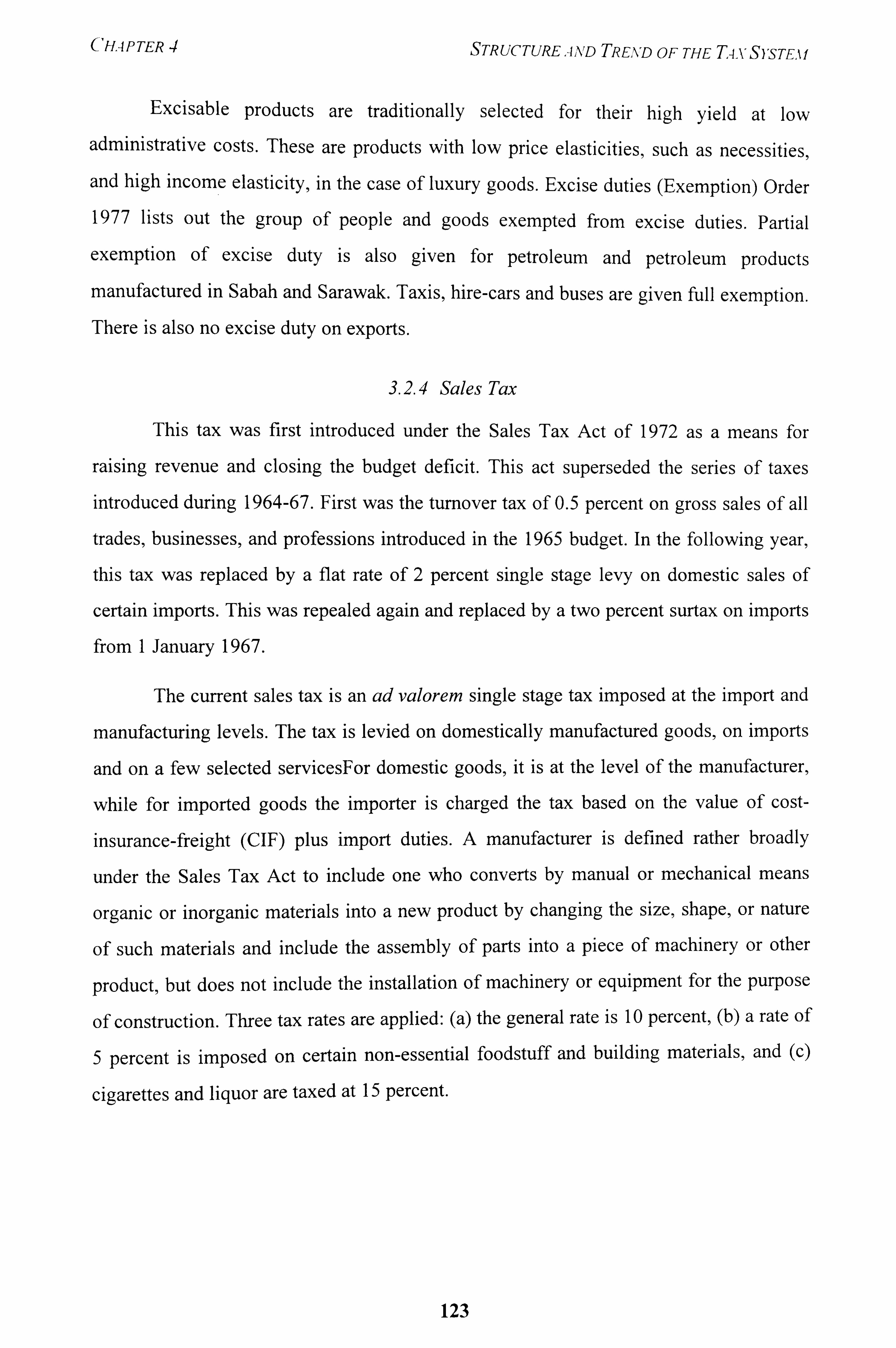
CHAPTER 4 STRUCTUREAND TREND OF THE T4. vS)'STEm

Excisable products are traditionally selected for their high yield at low

administrative costs. These are products with low price elasticities, such as necessities,

and high income elasticity, in the case of luxury goods. Excise duties (Exemption) Order

1977 lists out the group of people and goods exempted from excise duties. Partial

exemption of excise duty is also given for petroleum and petroleum products

manufactured in Sabah and Sarawak. Taxis, hire-cars and buses are given full exemption. There is also no excise duty on exports.

3.2.4 Sales Tax

This tax was first introduced under the Sales Tax Act of 1972 as a means for

raising revenue and closing the budget deficit. This act superseded the series of taxes

introduced during 1964-67. First was the turnover tax of 0.5 percent on gross sales of all

trades, businesses, and professions introduced in the 1965 budget. In the following year,

this tax was replaced by a flat rate of 2 percent single stage levy on domestic sales of

certain imports. This was repealed again and replaced by a two percent surtax on imports

from I January 1967.

The current sales tax is an ad valorem single stage tax imposed at the import and

manufacturing levels. The tax is levied on domestically manufactured goods, on imports

and on a few selected servicesFor domestic goods, it is at the level of the manufacturer,

while for imported goods the importer is charged the tax based on the value of cost-

insurance-freight (CIF) plus import duties. A manufacturer is defined rather broadly

under the Sales Tax Act to include one who converts by manual or mechanical means

organic or inorganic materials into a new product by changing the size, shape, or nature

of such materials and include the assembly of parts into a piece of machinery or other

product, but does not include the installation of machinery or equipment for the purpose

of construction. Three tax rates are applied: (a) the general rate is 10 percent, (b) a rate of

5 percent is imposed on certain non-essential foodstuff and building materials, and (c)

Cigarettes and liquor are taxed at 15 percent.

123

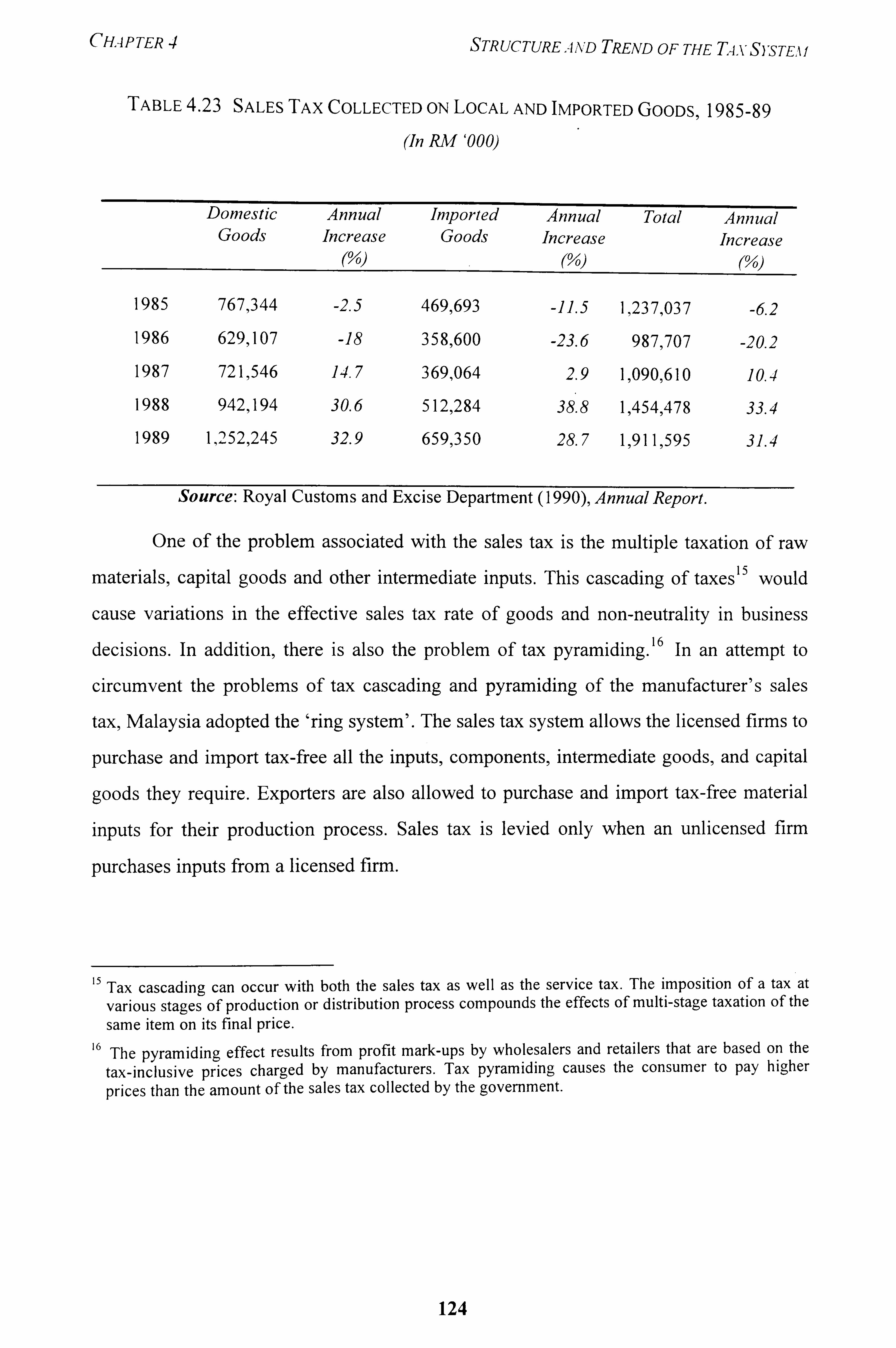
CHAPTER STRUCTURE, -iAD TREND OF THE T4, vS), sTE, v

TABLE 4.23 SALEs TAX COLLECTED ON LOCAL AND IMPORTED GOODS, 1985-89

(In RM '000)

Domestic Goods

Annual Increase

(0/0)

Imported Goods

Annual Increase

(0/0)

Total Annual Increase

(0/0)

1985 767,344 -2.5 4691693 -11.5 1,237,037 -62 1986 6291107 -18 358,600 -23.6 987,707 -20.2 1987 721,546 14.7 369,064 2.9 1,090,610 10.4

1988 942,194 30.6 512ý284 38 .8

1,454,478 33.4

1989 1,2521245 32.9 659,350 28.7 1,911 ý595 31.4

Source: Royal Customs and Excise Department (1990), Annual Report

One of the problem associated with the sales tax is the multiple taxation of raw

materials, capital goods and other intermediate inputs. This cascading of taxes' 5 would

cause variations in the effective sales tax rate of goods and non-neutrality in business

decisions. In addition, there is also the problem of tax pyramiding. 16 In an attempt to

circumvent the problems of tax cascading and pyramiding of the manufacturer's sales

tax, Malaysia adopted the 'ring system'. The sales tax system allows the licensed firms to

purchase and import tax-free all the inputs, components, intermediate goods, and capital

goods they require. Exporters are also allowed to purchase and import tax-free material

inputs for their production process. Sales tax is levied only when an unlicensed firm

purchases inputs from a licensed firm.

15 Tax cascading can occur with both the sales tax as well as the service tax. The imposition of a tax at various stages of production or distribution process compounds the effects of multi-stage taxation of the same item on its final price.

16 The pyramiding effect results from profit mark-ups by wholesalers and retailers that are based on the tax-inclusIve prices charged by manufacturers. Tax pyramiding causes the consumer to pay higher

prices than the amount of the sales tax collected by the government.

124

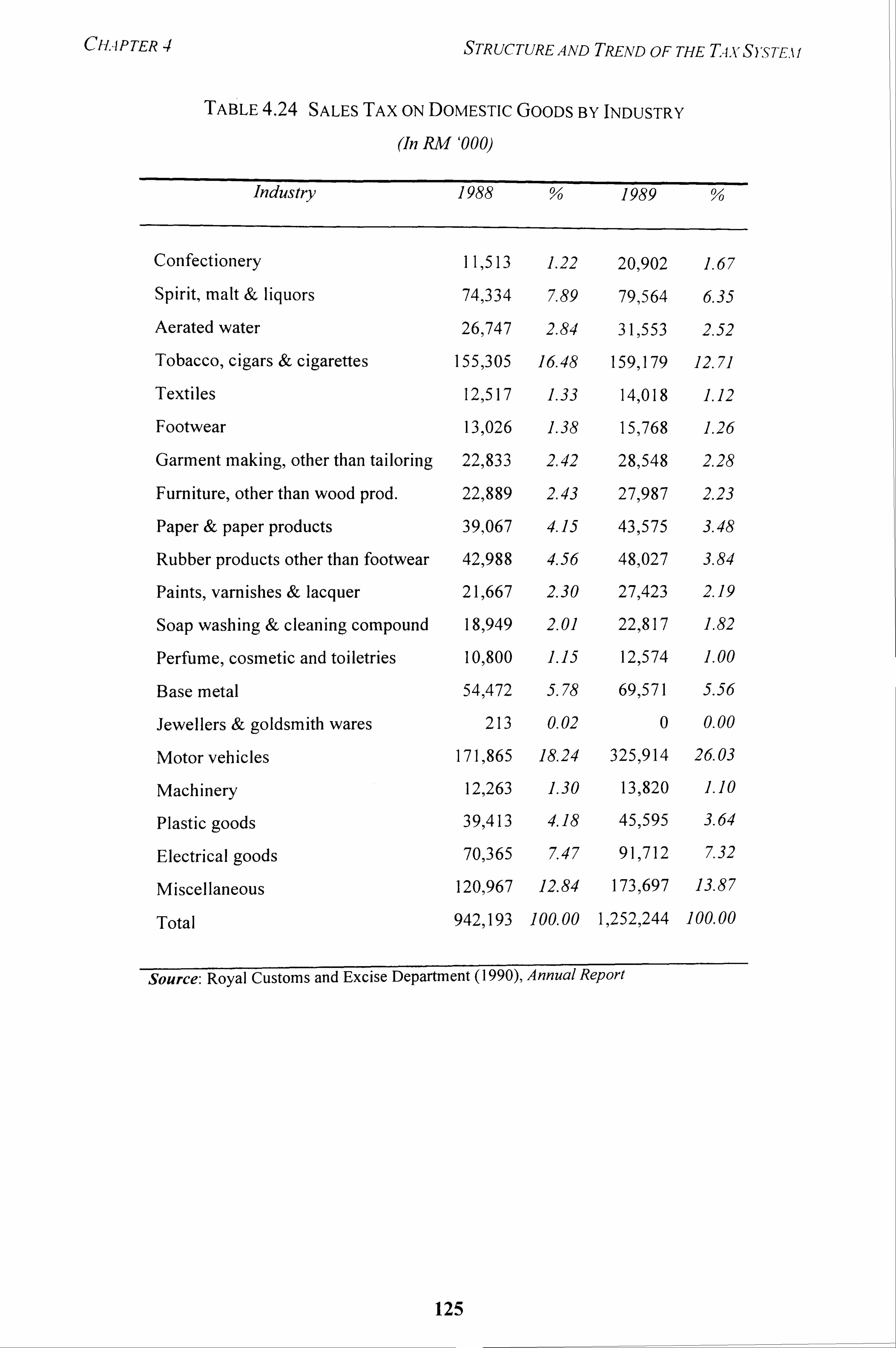
CHAPTER 4 STRUCTURE AND TREND OF THE TIVS)STEI I

TABLE 4.24 SALES TAX ON DOMESTIC GOODS BY INDUSTRY

(In RM '0 0 0)

Industry 1988 % 1989 %

Confectionery

Spirit, malt & liquors

Aerated water

Tobacco, cigars & cigarettes

Textiles

Footwear

Garment making, other than tailoring

Furniture, other than wood prod.

Paper & paper products

Rubber products other than footwear

Paints, varnishes & lacquer

Soap washing & cleaning compound

Perfume, cosmetic and toiletries

Base metal

Jewellers & goldsmith wares

Motor vehicles

Machinery

Plastic goods

Electrical goods

Miscellaneous

Total

11,513 1.22 20,902 1.67

74,334 7.89 79,564 6.35

26,747 2.84 31ý553 2.52

155,305 16.48 159,179 12.71

12,517 1.33 14,018 1.12

13,026 1.38 15,768 1.26

221833 2.42 28,548 2.28

22,889 2.43 271987 2.23

39,067 4.15 439575 3.48

42,988 4.56 48,027 3.84

21,667 2.30 27,423 2.19

18,949 2.01 22e817 1.82

10,800 1.15 123574 1.00

54,472 5.78 69,571 5.56

213 0.02 0 0.00

171,865 18.24 325,914 26.03

12,263 1.30 139820 1.10

39,413 4.18 453595 3.64

70,365 7.47 91,712 7.32

120,967 12.84 1731697 13.87

9421193 100.00 1 e252e244 100.00

Source: Royal Customs and Excise Department (1990), Annual Report

125

CHAPTER STR UC TURE A ND TREND OF THE T4X S)'s TE, ý i

Manufacturers whose sale value of taxable goods do not exceed RM100,000 per

annum are exempted from sales tax to keep the tax administration manageable. To

promote vertical equity tax and not overburden the poor households, the sales tax

exempts primary commodities, basic foodstuffs, basic building materials, and certain

agricultural implements and machinery. Luxury goods are subject to higher taxes.

However, the net effect of the sales tax is not really progressive throughout the income

scale. According to Salleh (1988), the distribution of sales tax burden of locally

manufactured and imported goods is regressive for the lower income bracket but

progressive at the upper income bracket. In addition, certain tourist and sports goods, books, newspapers and other reading materials and all exports are exempted from sales

tax. Certain privileged persons, diplomats and government agencies are not required to

pay the tax.

During the last twenty years, the contribution of sales tax to total tax revenue

grew from 6 percent in 1975 to II percent in 1995. This is a modest growth considering

the rapid expansion of consumption of II percent per annum during 1975-95. The

government had taken steps to improve the sales tax and the service tax. In 1983, the

sales tax rate was increased from 5 to 10 percent and tobacco and liquor products were

taxed at 15 percent. The base of sales tax was expanded with the removal of a few

exemptions in 1988. In the 1989 Budget, the sales tax was re-imposed on certain

foodstuffs, building materials, semi-processed and non-essential goods. Table 4.23 shows

the revenue collected from sales tax on local and imported goods, while Table 4.24

presents the structure of sales tax on domestic goods by industry for 1988 and 1989.

Despite these adjustments, the narrow base and problems associated with the sales tax

remain because the system is basically flawed.

3.2.5 Service Tax

This tax was introduced under the Service Tax Act, 1975. A service tax of 5 percent is

imposed on certain goods and services provided in certain prescribed establishments. The

goods are food, drinks and tobacco, while the main services include rooms for lodging,

nightclubs, dance halls, cabarets, health centres and massage parlours. Generally, all

large hotels and their restaurants are subject to the tax. A limited range of restaurants

located outside hotels are also subjected to the tax provided their annual turnover exceed

126

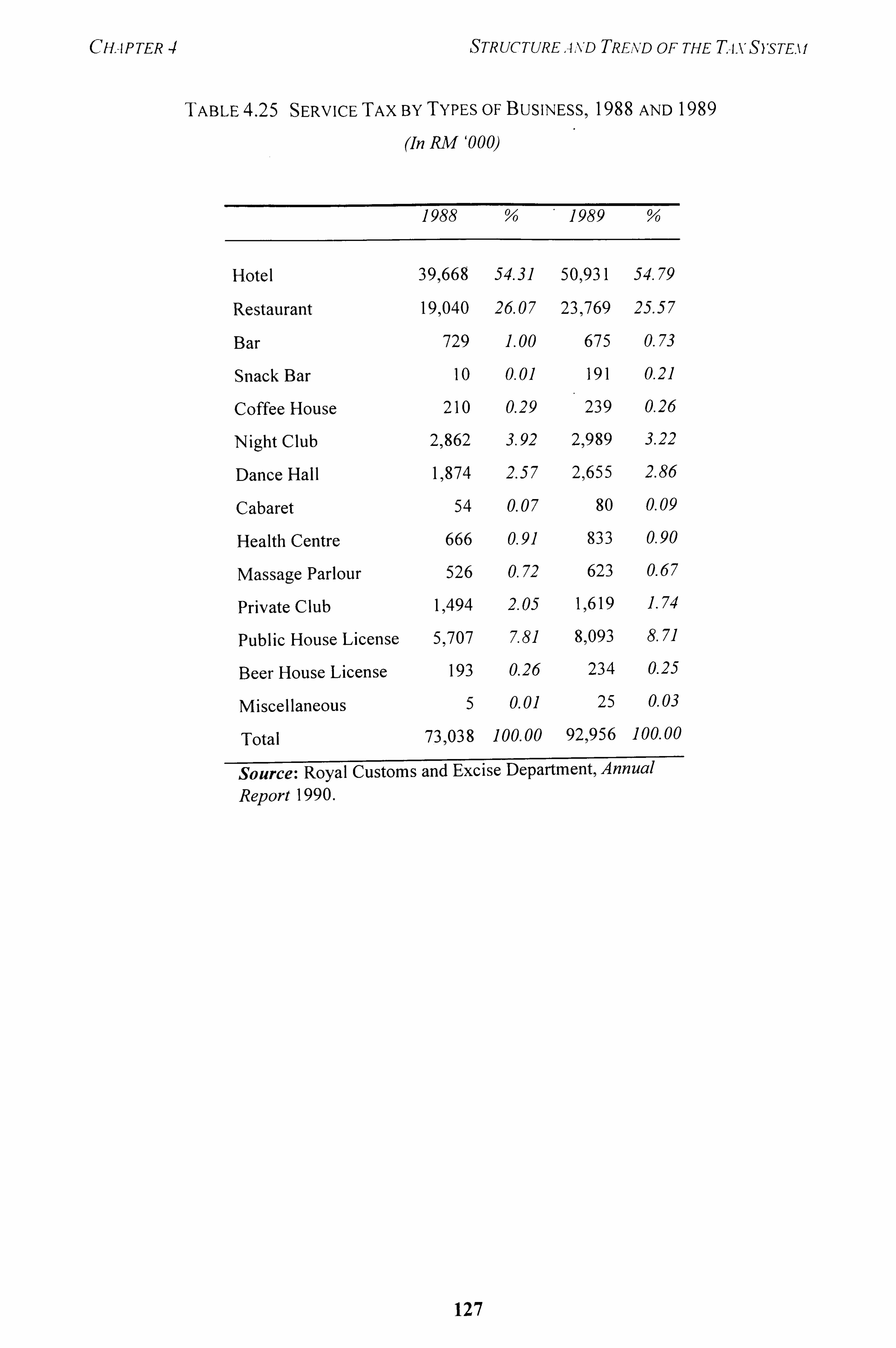
CHAPTER 4 STRUCTUREAND TREAV OF THE T. -i. ý'S), sTE. ýi

TABLE 4.25 SERVICE TAX By TYPES OF BUSINESS, 1988 AND 1989

(In RM '0 0 0)

1988 %' 1989 %

Hotel 39,668 54.31 505931 54.79

Restaurant 19,040 26.07 23,769 25.57

Bar 729 1.00 675 0.73

Snack Bar 10 0.01 191 0.21

Coffee House 210 0.29 239 0.26

Night Club 21862 3.92 21989 3.22

Dance Hall 1,874 2.57 2,655 2.86

Cabaret 54 0.07 80 0.09

Health Centre 666 0.91 833 0.90

Massage Parlour 526 0.72 623 0.67

Private Club 1 ý494 2.05 1 fi19 1.74

Public House License 51707 7.81 8ý093 8.71

Beer House License 193 0.26 234 0.25

Miscellaneous 5 0.01 25 0.03

Total 73,038 100-00 921,956 100.00

Source: Royal Customs and Excise Department, Annual Report 1990.

127

CHAPTER 4 STRUCTURE AND TREND OF THE T-I-VSYSTEll

RM500ý000. All places in possession of first class liquor licenses have also been brought

within the ambit of this tax. However, the tax does not apply to hotels having less than 25 rooms, hostels for students or those maintained by religious institutions, as well as restaurants with less than RM500,000 annual turnover and located outside hotels. As

shown in Table 4.25, about 80 percent of the service tax revenue for 1988 and 1989 were derived from hotels and restaurants.

The service tax has subsequently been widened in recent budgets. In the 1992 Budget, the tax covers professional and consultancy services provided at private hospitals and by legal, engineering, surveyor, architectural, accounting and other consultancy firms having an annual sales turnover of RM300,000 and above. In addition, services provided by advertising firms, insurance companies and motor vehicles service

and repair centres, and forwarding agents are subject to service tax. In the 1994 Budget,

the tax was further widened to include courier, parking bay, dental and veterinary

services. Despite the extension of the service tax, its contribution to total tax revenue is

small, at only 2 percent in 1995.

3.3 Weaknesses ofSales and Service Taxes

The sales tax as it stands provides tremendous scope for tax evasion. The task of

administering the sales tax is complex and intractable both for the manufacturers as well

as the Royal Customs and Excise Department that collects the taxes. Over 3,000 items

and 100 categories of manufacturers are exempted from the tax. Since the tax is levied at

the manufacturer/import level, manufacturers are encouraged to reduce tax liabilities

through transfer pricing by shifting the tax base to the wholesale and retail arm. Taxing

at the pre-retail level causes problems because of the difficulty in distinguishing final

goods from intermediate goods. As an indicator of tax evasion among manufacturers, an

increase of 100 percent in sales tax in 1983 from 5 percent to 10 percent had resulted in

only an increase of 63 percent in tax revenue.

In addition, tax officials face problems assessing the amount of tax due from

manufacturers that produce a wide variety of products, some of which are tax exempted

and others may be taxed at different rates. There is no mechanism in the sales and service

taxes to remove tax cascading from exports, which places Malaysian exports at a

128

CHAPTER 4 STRUCTURE. 4ND TREATD OF THE T4. vS)'STE. Ii

disadvantage. For Malaysian exports to be competitive at the international market, merchandise exports should not be taxed either explicitly or implicitly. The pyramiding and cascading of taxes affects prices of goods differently and in a manner unintended by policy makers, besides raising the cost of living.

3.3.1 Rationale For Adopting VAT

To overcome some of the weaknesses of the current sales and service taxes, the Malaysian Government is currently considering the adoption of a version of the value added tax (VAT). This intention was expressed in the 1989 Budget Speech and again in the 1993 Budget Speech. When Malaysia adopts the value added tax, it will join the ranks of over fifty-five industrial and developing countries that have implemented this

system since the 1960s. According to Cnossen (1991: 72), VAT can generate revenues of around 0.4 percent of GDP for every percentage point of the rate, which might be useful in providing the government with an indirect tax handle to raise revenue. The advantage of VAT over the existing sales and service taxes is its neutrality. The tax does not interfere with production or trade, and does not distort the economic costs of doing

business. Malaysian exports can be tax exempted and become more competitive internationally. It also reduces tax evasion with its self-policing feature of using a system

of credits.

There are other advantages for Malaysia in adopting the VAT system. VAT will

extend the tax base and generate more revenue to counteract the fall in the rates of many

of the taxes. The removal of tax cascading and tax pyramiding is expected to improve the

investment climate for local and foreign businesses, as well as free business from the

burden of applying for tax exemptions from the Royal Customs and Excise Department.

One area of concern is that the adoption of VAT may lead to increased price level.

Narayanan (1991: 85) argues that the price level will rise if VAT brings in more revenue

than sales tax, and if traders widen the profit margin to protect themselves against

uncertainty. However, Tait (1990: 18) found that among 36 countries that adopted VAT,

22 countries had a negligible price effect, eight countries experienced a one-time price

increase, and six countries experienced an increase in their inflation rates. Gillis, Shoup

and Sicat (1990: 22 1) conclude that other factors may lead to inflation, but not VAT.

129

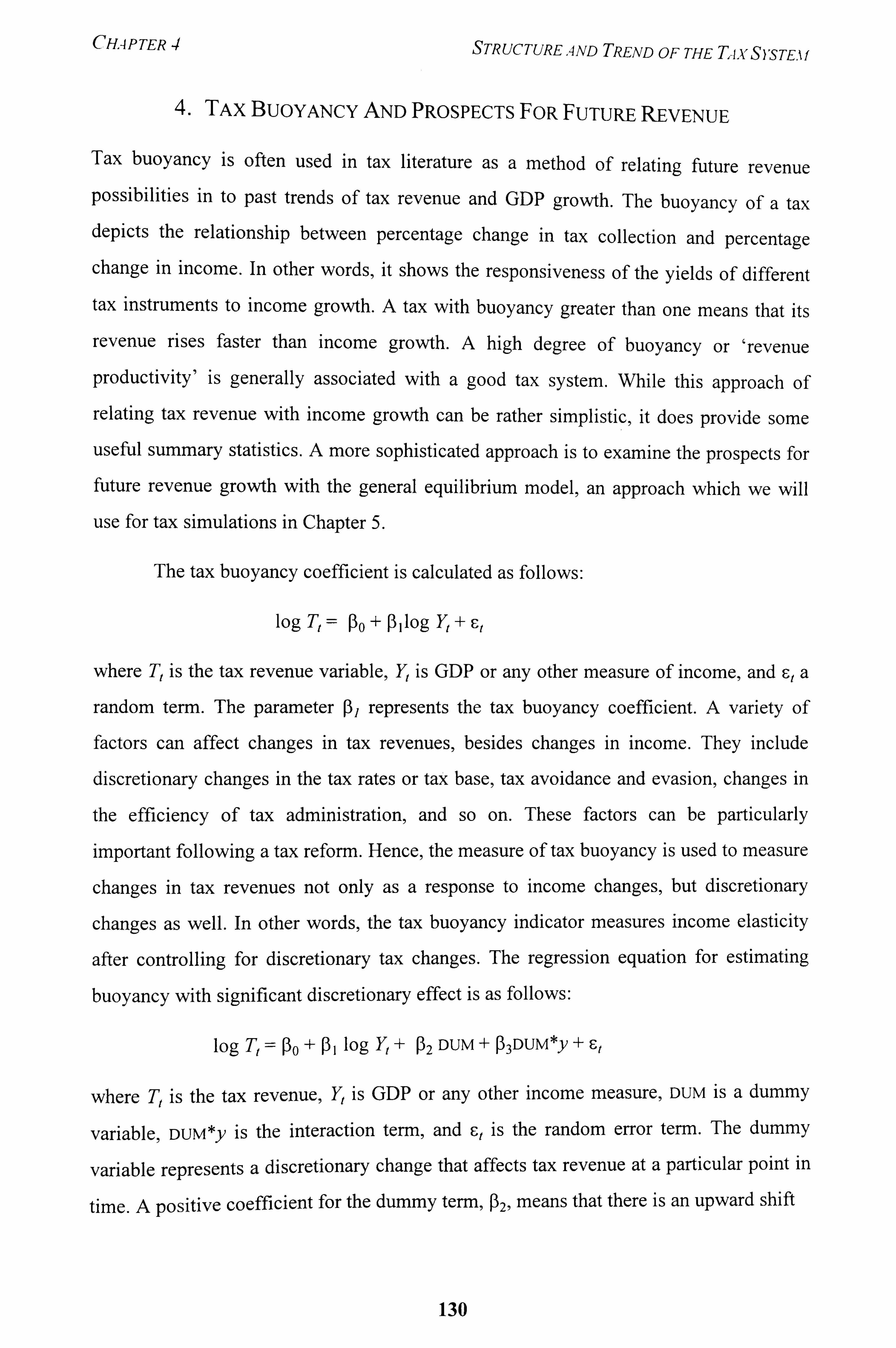
CHAPTER 4 STRUCTUREAND TREND OF THE T, -i. VS)'STE. If

4. TAx BUOYANCY AND PROSPECTs FOR FUTURE REVENUE

Tax buoyancy is often used in tax literature as a method of relating future revenue possibilities in to past trends of tax revenue and GDP growth. The buoyancy of a tax depicts the relationship between percentage change in tax collection and percentage change in income. In other words, it shows the responsiveness of the yields of different

tax instruments to income growth. A tax with buoyancy greater than one means that its

revenue rises faster than income growth. A high degree of buoyancy or 'revenue

productivity' is generally associated with a good tax system. While this approach of relating tax revenue with income growth can be rather simplistic, it does provide some useful summary statistics. A more sophisticated approach is to examine the prospects for future revenue growth with the general equilibrium model, an approach which we will use for tax simulations in Chapter 5.

The tax buoyancy coefficient is calculated as follows:

log T, = PO + p1log Yt + F,

where T, is the tax revenue variable, Y, is GDP or any other measure of income, and E, a

random term. The parameter P, represents the tax buoyancy coefficient. A variety of

factors can affect changes in tax revenues, besides changes in income. They include

discretionary changes in the tax rates or tax base, tax avoidance and evasion, changes in

the efficiency of tax administration, and so on. These factors can be particularly

important following a tax reform. Hence, the measure of tax buoyancy is used to measure

changes in tax revenues not only as a response to income changes, but discretionary

changes as well. In other words, the tax buoyancy indicator measures income elasticity

after controlling for discretionary tax changes. The regression equation for estimating

buoyancy with significant discretionary effect is as follows:

109 Tt = PO +P1 109 yt + P2 DUM + P3DUM*y + Et

where T, is the tax revenue, Y, is GDP or any other income measure, DUM is a dummy

variable, DUM*y is the interaction term, and E;, is the random error term. The dummy

variable represents a discretionary change that affects tax revenue at a particular point in

time. A positive coefficient for the dummy term, P2, means that there is an upward shift

130

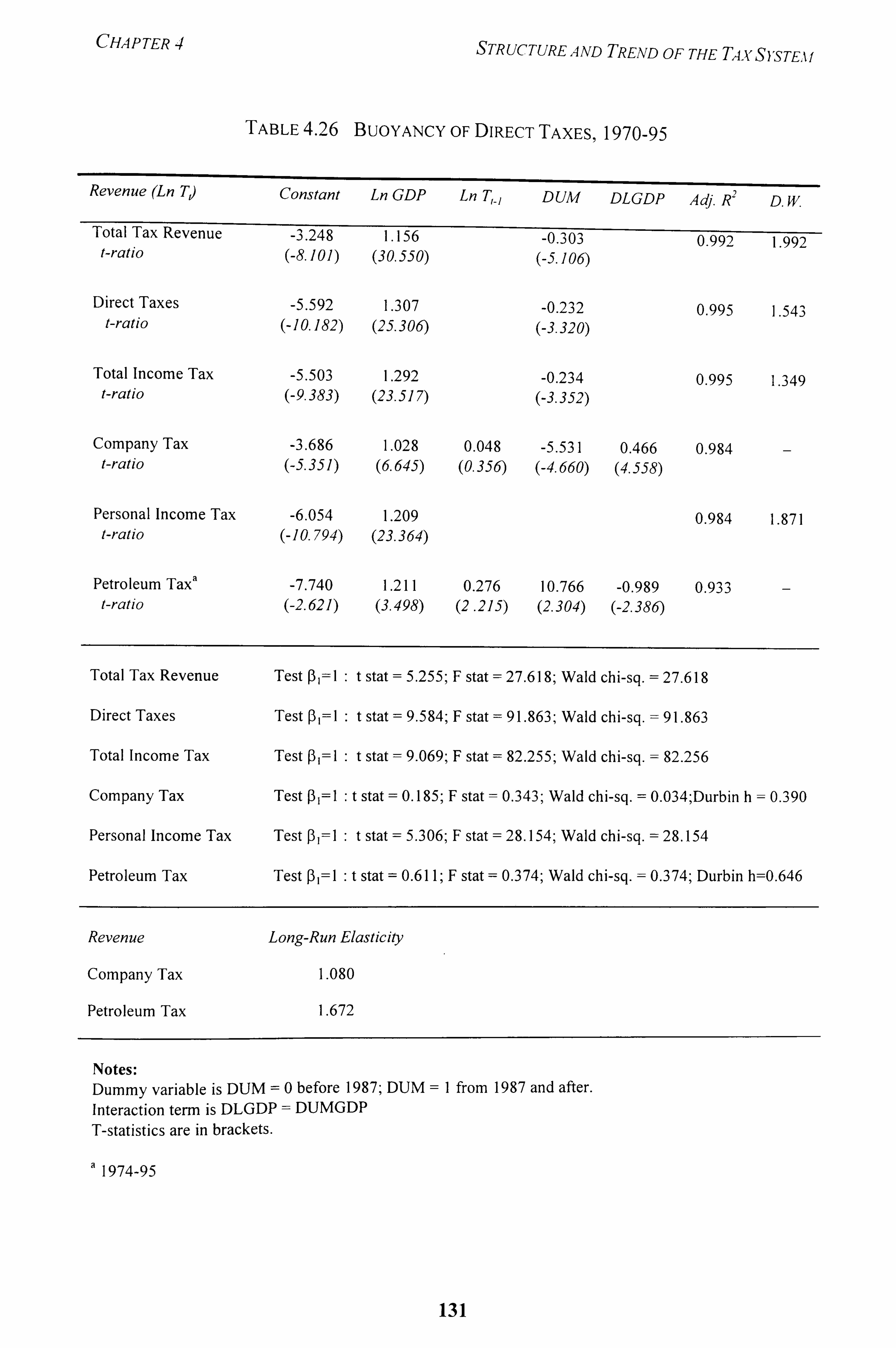
CHAPTER 4 STRUCTURE AND TREND OF THE TA-v S), sTE, i f

TABLE 4.26 BUOYANCY OF DIRECT TAXES, 1970-95

Revenue (Ln Td Constant Ln GDP Ln T, -,

DUM DLGDP Adj. R2D. W.

Total Tax Revenue t-ratio

-3.248 (-8-101)

1.156 (30.550)

-0.303 0.992 1.992- (-5.106)

Direct Taxes -5.592 1.307 -0.232 t-ratio (-10.182) (25.306) (-3.320)

Total Income Tax -5.503 1.292 -0.234 t-ratio (-9.383) (23.517) (-3.352)

Company Tax -3.686 1.028 0.048 -5.531 0.466 t-ratio (-5.351) (6.645) (0.356) (4.660) (4.558)

Personal Income Tax -6.054 1.209 t-ratio (-10.794) (23.364)

Petroleum Tax a -7.740 1.211 0.276 10.766 -0.989

t-ratio (-2.621) (3.498) (2.215) (2.304) (-2.386)

0.995 1.5433

0.995 1.349

0.984

0.984 1.871

0.933

Total Tax Revenue Test P, =I t stat = 5.255; F stat = 27.618; Wald chi-sq. = 27.618

Direct Taxes Test P1=1 t stat = 9.584; F stat = 91.863; Wald chi-sq. = 91.863

Total Income Tax Test P, =l t stat = 9.069; F stat = 82.255; Wald chi-sq. = 82.256

Company Tax Test P1=1 t stat 0.185; F stat 0.343; Wald chi-sq. = 0.034; Durbin h=0.390

Personal Income Tax Test P, =] t stat 5.306; F stat 28.154; Wald chi-sq. = 28.154

Petroleum Tax Test P1=1 t stat 0.611; F stat = 0.374; Wald chi-sq. = 0.374; Durbin h=0.646

Revenue Long-Run Elasticity

Company Tax 1.080

Petroleum Tax 1.672

Notes: Dummy variable is DUM =0 before 1987; DUM =I from 1987 and after. Interaction term is DLGDP = DUMGDP T-statistics are in brackets.

1974-95

131

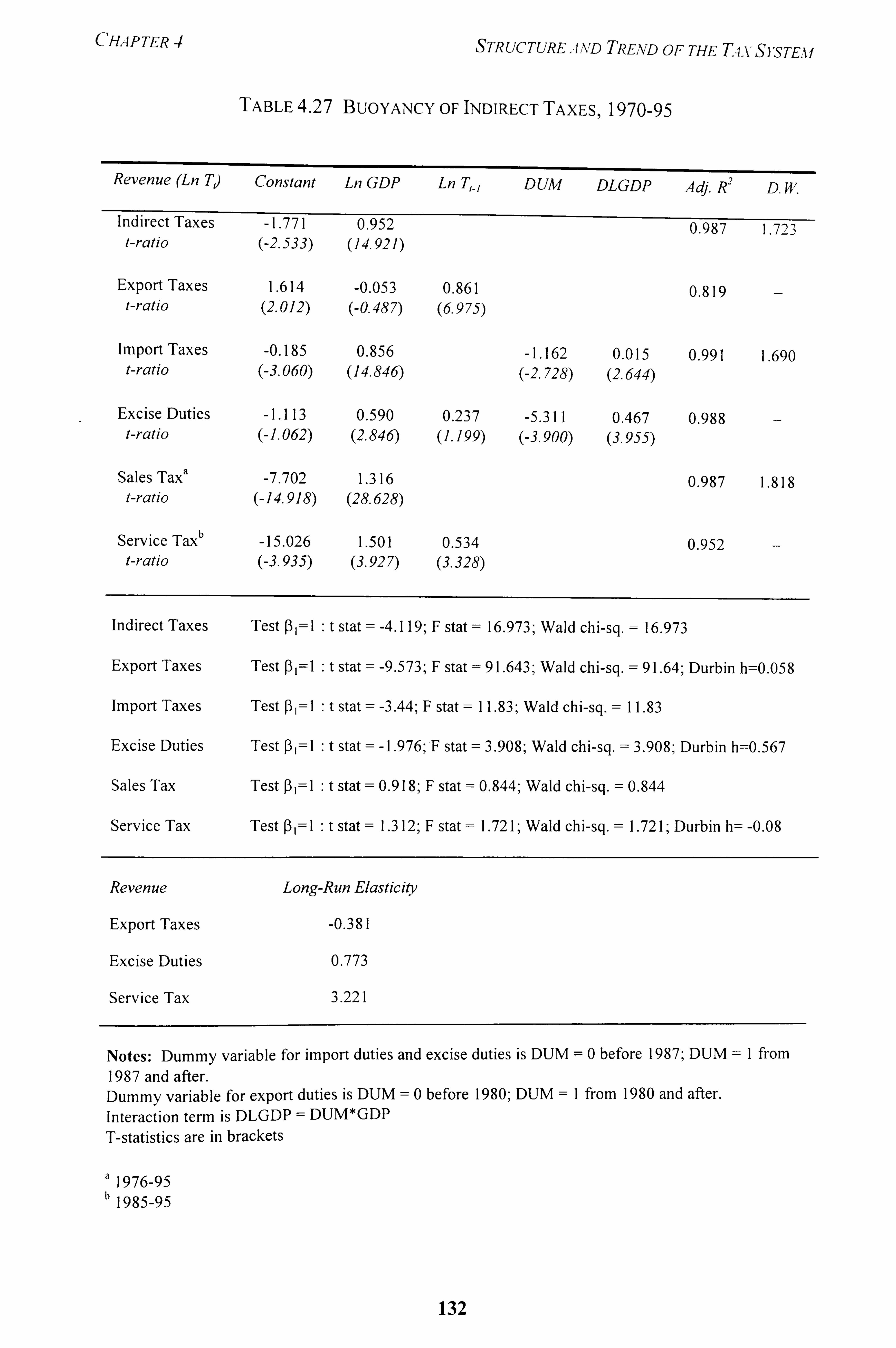
CHA P TE R4 STRUCTURE . 4ND TREND OF THE TAx S), sTEAf

TABLE 4.27 BUOYANCY OF INDIRECT TAXES, 1970-95

Revenue (Ln Td Constant Ln GDP Ln T, -,

DUM DLGDP Adj. R2 D. 14'.

Indirect Taxes -1.771 0.951 0.987 1.7233 t-ratio (-2.533) (14.921)

Export Taxes 1.614 -0.053 0.861 0.819 - t-ratio (2.012) (-0.487) (6.975)

Import Taxes -0.185 0.856 -1.162 0.015 0.991 1.690 t-ratio (-3.060) (14.846) (-2.728) (2.644)

Excise Duties -1.113 0.590 0.237 -5.311 0.467 0.988 - t-ratio (-1.062) (2.846) (1.199) (-3.900) (3.955)

Sales Tax a -7.702 1.316 0.987 1.818

t-ratio (-14.918) (28.628)

Service Tax b

-15.026 1.501 0.534 0.952 - t-ratio (-3-935) (3.927) (3.328)

Indirect Taxes Test P1=1 t stat = -4.119; F stat = 16.973; Wald chi-sq. = 16-973

Export Taxes Test P1=1 t stat = -9.573; F stat = 91.643; Wald chi-sq. = 91.64; Durbin h =0.058

Import Taxes Test P1=1 t stat = -3.44; F stat = 11.83; Wald chi-sq. = 11.83

Excise Duties Test P, =I t stat = -1.976; F stat = 3.908; Wald chi-sq. = 3.908; Durbin h= 0.567

Sales Tax Test Pj=I t stat = 0.918; F stat = 0.844; Wald chi-sq. = 0.844

Service Tax Test P, =1 t stat = 1.312; F stat = 1.721; Wald chi-sq. = 1.721; Durbin h= -0.08

Revenue Long-Run Elasticity

Export Taxes -0.381

Excise Duties 0.773

Service Tax 3.221

Notes: Dummy variable for import duties and excise duties is DUM =0 before 1987; DUM =I from 1987 and after. Dummy variable for export duties is DUM =0 before 1980; DUM =I from 1980 and after. Interaction terin is DLGDP = DUM*GDP T-statistics are in brackets

a 1976-95 b 1985-95

132

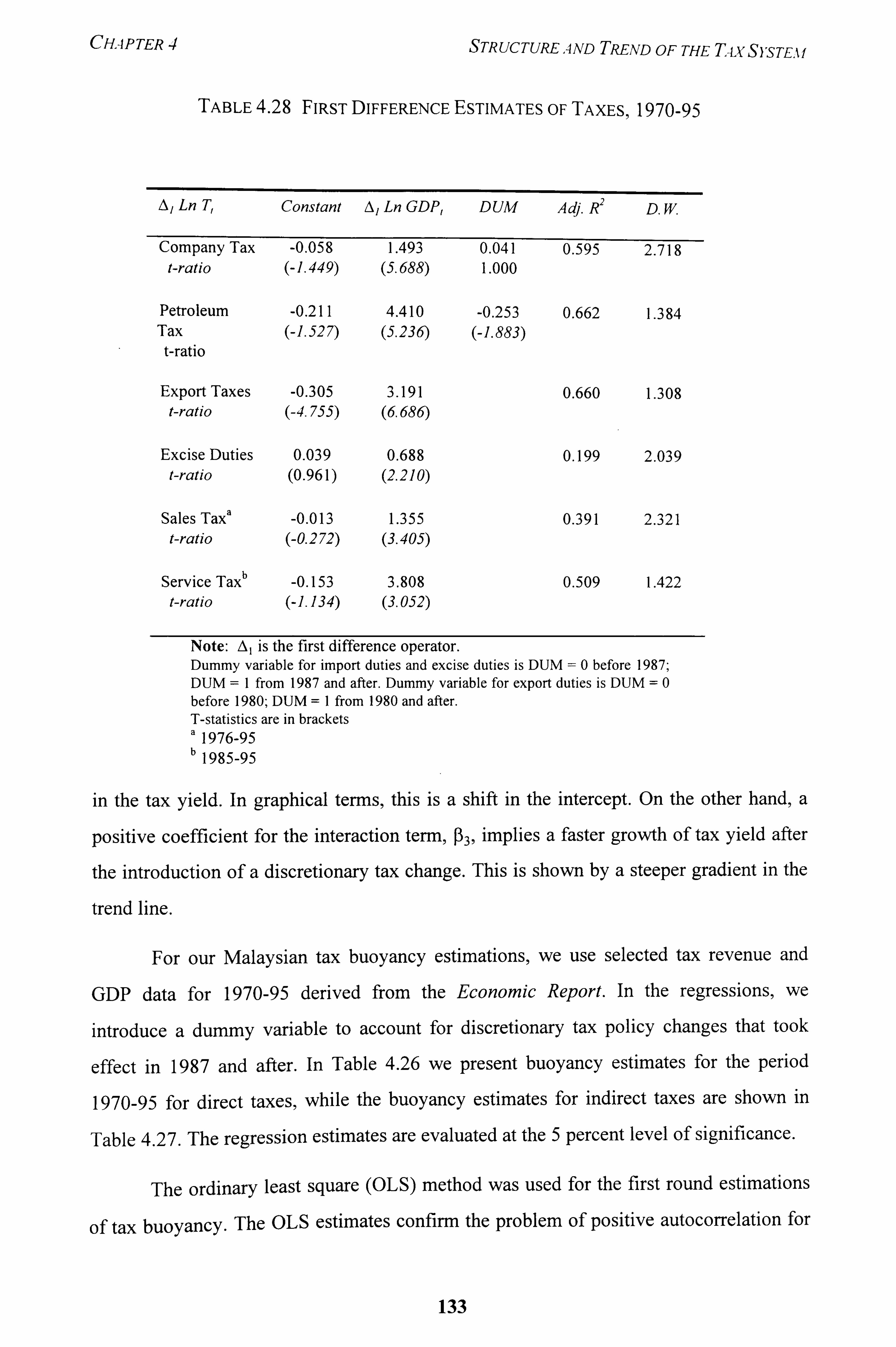
CHAPTER 4 STRUCTURE. 4ND TREND OF THE TA-vSYSTEM

TABLE 4.28 FIRST DIFFERENCE ESTIMATES OF TAXES, 1970-95

A/ Ln T, Constant A, Ln GDP, DUM Adj. R2D. W.

Company Tax -0.058 1.493 0.041 0.595 2.718 t-ratio (-1.449) (5.688) 1.000

Petroleum -0.211 4.410 -0.253 0.662 1.384 Tax (-1.527) (5.236) (-1.883) t-ratio

Export Taxes -0.305 3.191 0.660 1.308 t-ratio (-4.755) (6.686)

Excise Duties 0.039 0.688 0.199 2.039 t-ratio (0.961) (2.210)

Sales Tax a -0.013 1.355 0.391 2.321 t-ratio (-0.272) (3.405)

Service Tax b -0.153 3.808 0.509 1.422

t-ratio (-1.134) (3.052)

Note: A, is the first difference operator. Dummy variable for import duties and excise duties is DUM =0 before 1987; DUM =I from 1987 and after. Dummy variable for export duties is DUM =0 before 1980; DUM =I from 1980 and after. T-statistics are in brackets a 1976-95 b

1985-95

in the tax yield. In graphical terms, this is a shift in the intercept. On the other hand, a

positive coefficient for the interaction term, P3, implies a faster growth of tax yield after

the introduction of a discretionary tax change. This is shown by a steeper gradient in the

trend line.

For our Malaysian tax buoyancy estimations, we use selected tax revenue and

GDP data for 1970-95 derived from the Economic Report. In the regressions, we

introduce a dummy variable to account for discretionary tax policy changes that took

effect in 1987 and after. In Table 4.26 we present buoyancy estimates for the period

1970-95 for direct taxes, while the buoyancy estimates for indirect taxes are shown in

Table 4.27. The regression estimates are evaluated at the 5 percent level of significance.

The ordinary least square (OLS) method was used for the first round estimations

of tax buoyancy. The OLS estimates confirm the problem of positive autocorrelation for

133

CHAP TER -1 STRUCTURE -4AD TREND OF THE Tqx S) sTE, ý f

The ordinary least square (OLS) method was used for the first round estimations of tax buoyancy. The OLS estimates confirm the problem of positive autocorrelation for many of the regression equations, as indicated by their Durbin-Watson d statistics falling below the lower critical limit 1.302 at 5 percent level of significance. 17 To correct for autocorrelation, we used two approaches: (a) the Cochrane-Orcutt iterative method with convergence at 0.001, and (b) auto regressive lagged dependent variable approach. This

process brought an improvement to the Durbin-Watson statistics for all the estimations using the Cochrane-Orcutt method, although some of the regression models had DW

statistics falling within the region of indecision. For the taxes modelled on the auto regressive approach, we have also estimated the coefficients using the first difference

approach and presented the Durbin h statistics, as shown in Table 4.28.

In our buoyancy estimations for direct income taxes, the tax revenue for any particular year is regressed against the GDP figures for the previous year in order to take

into account Malaysia's prior-year assessment system. In other words, current year tax

collection is based on last year's income assessment. In the case of indirect taxes, tax

revenues are regressed against the GDP figures of corresponding years. The estimation

used data from 1970-95, except for those taxes with shorter data series.

4.1 Tax Buo ancy Estimates y

The results of the tax buoyancy estimations are shown in Table 4.26 and Table

4.27. The buoyancy coefficient for total tax revenue is 1.1, which means that the increase

in tax revenue is a little greater in proportionate terms than the increase in income. Direct

taxes are more buoyant than indirect taxes, a factor which accounts for the growing share

of direct taxes in government revenue. After controlling for discretionary tax changes

with the dummy variable, an increase in GDP by I percent would be accompanied with a

corresponding increase of 1.3 percent for direct taxes and 0.9 percent for indirect taxes.

Among the components of direct taxes, personal income tax and petroleum tax

have buoyancy coefficients of 1.2, while corporate tax has a unitary buoyancy

17 In the presence of autocorrelation, the OLS estimators remain unbiased and consistent, but they are no longer efficient. This means that the usual standard error, t and F tests of significance are not dependable.

134

CHAPTER 4 STRUCTURE, 4ND TREATD OF THE T4. VSYSTEAl

coefficient. However, the test for the hypothesis PI=I shows that the buoyancy for petroleum and corporate taxes are no different from one. The absence of a dummy

variable in the personal income tax model suggests that the revisions in the marginal personal income tax rates during the late eighties and early nineties have had negligible effect on the overall revenue productivity of this tax. The relatively low buoyancy of company tax may come as a surprise in view of Malaysia's rapidly growing economy and corporate sector. This could only imply that the wide range of tax exemption and incentives for the manufacturing sector had a more important role in dampening tax

revenue expansion than was generally realised.

Table 4.27 shows that the buoyancy coefficient for indirect taxes is less than one. In other words, if the trend continues into the future, indirect taxes will not be very

productive in revenue generation, unlike direct taxes. An examination of the component

taxes reveals why this is the case. The buoyancy coefficient of export tax is practically

zero, as shown by the insignificant coefficient for LNGDP at the 5 percent level. This

comes as no surprise since export tax revenue for 1986-95 were fluctuating around the

1976-79 levels. Both import tax and excise duties have buoyancy coefficients of less than

unitary. Among the indirect taxes, only the sales tax and service tax, which underwent

expansion in their tax bases, had buoyancy coefficients of 1.3 and 1.5, respectively. The

regression shows that service tax has a relatively high long-run elasticity of 3.2, but the

period is too short for it to be really meaningful. Since sales and service taxes contribute

slightly over a quarter of the indirect tax revenue, their higher buoyancy coefficients are

not large enough to influence the low buoyancy for indirect taxes.

4.2 Issues on Tax Reform

Despite their limitations and the caveats on using them as guidance for policy, 18

tax buoyancy comparisons can be revealing in a number of ways. First, they provide

some idea about the tax revenue trajectories. In raising revenue, the government could

either focus on the taxes that are more responsive to GDP growth or, alternatively,

18 Buoyancy estimates are based on past behaviour. They would not necessarily be good indicators of future revenue if the tax rates and structure are modified.

135

CHAPTER 4 STRUCTURE, 4,, NiD TREND oF THE Tq. VS), STE. u

examine the areas of weakness in the tax structure. The latter would imply taking steps to reform the tax structure.

Second, in some of the regressions, the introduction of dummy variables helps to

explain the role of discretionary tax changes that influence the revenue trend of revenue

collected from these taxes since 1987, which are related to several tax reforms adopted in

Malaysia. The corporate income rate was reduced in stages starting from 1986 as a

means to stimulate investment and keep abreast with the corporate tax regimes of

neighbouring countries. With the adoption of the Promotion of Investment Act (PIA)

1986,, investment incentives and tax allowances for the manufacturing sector were

expanded. For the petroleum industry, the Second Generation Production Sharing

Contracts were adopted to provide more favourable terms and greater incentives to the

contractor. The government also started to reduce gradually excise and import duties as a

means of keeping consumer prices down and relieving the tax burden on the poor.

Among one of the most comprehensive and influential non-governmental proposals for

tax reform in Malaysia are contained in a report entitled, 'A Tax Reform Package for

Malaysia' (MIER, 1988). This report presents the recommendations of the Colloquium

on Tax Reform organised by the Malaysian Institute of Economic Research, which was

attended by representatives from professional associations and business organisations,

tax consultants, consumer groups, trade unions and academicians. Many of the proposals

from the colloquium. have been adopted by the Malaysian government.

Third, the estimates show that the petroleum buoyancy coefficient is slightly

above unitary. Petroleum has provided the tax base for the eighties and early nineties.

Since the tax revenue derived from petroleum is determined by fluctuating world oil

prices as well as production quotas laid out in the National Depletion Policy, much less

reliance should be placed on this natural resource sector to provide the impetus for public

revenue growth, at least not on the scale that it had demonstrated in the past. Therefore,

one of the themes for tax reform in Malaysia is the distribution of the tax burden, which

increasingly have to be shouldered by income and consumption taxes.

Fourth, the buoyancy coefficient for personal income tax shows that it is fairly

productive in revenue. Although Malaysia seems to perform favourably in comparison

with its neighbours in mobilising income tax revenue, its performance is still lower than

136

CHAPTER 4 STRUCTUREAND TREND OF THE T-ixSi'STE, ýi

the OECD countries. An avenue to increase personal income tax revenue is establishing a modem and efficient tax administration that increases the tax base through more effective assessment and collection mechanisms.

Fifth, the performance of corporate taxation, as reflected by the unitary buoyancy

coefficient, is not in keeping with the rapid expansion of the corporate sector. As an

indication of the dynamic corporate sector, private capital expenditure rose from

RML, 720 in 1988 to an estimated RM10,162 in 1994 (Ministry of Finance, 1994),

recording an average annual growth of 34 percent. Although corporate tax contributed a

growing share of the tax revenue, this relatively lacklustre performance of corporate tax

can be traced to the income tax revenue loss from the numerous business incentives to

attract foreign direct investments.

Finally, it highlights the fact that direct taxes are more productive in revenue

generation than indirect taxes. It does appear that in a tax reform, much more attention

should be given to redress the weaknesses of indirect taxes. The decline in trade taxes in

Malaysia is dictated by policy and is consistent with the trend shown in Singapore,

Thailand and Indonesia. Relative to the tax structures of Singapore, Indonesia and

Thailand discussed earlier in the chapter, Malaysia recorded a sharp decline in the share

of goods and services tax revenue despite the dynamism in business activities and private

consumption. In view of these patterns, we propose that the scope for increasing the

productivity of indirect taxes is to improve the current sales and service taxes by way of

adopting the value added tax (VAT), which would increase revenue and raise the

efficiency and equity of the tax system.

We take up some of these issues in the next chapter. By using the computable

general equilibrium model, we examine the macroeconomic effects of raising revenue

from personal income tax and corporate tax, compared to using the other indirect taxes to

raise the same amount of revenue. In addition, we measure the macroeconomic impact of

adopting VAT both as a revenue-neutral tax reform to replace the current sales and

service taxes, as well as a revenue-enhancing measure.

137

CHAPTER 4 STRUCTURE. AAD TREATD OF THE T-Lk'S)'STEm

5. CONCLUSION

During the last 25 years, the structure of the Malaysian tax system has changed quite dramatically. As shown by the tax buoyancy estimates., the tax reforms adopted after 1986 have had an impact on the revenue trends for some of the taxes. Although indirect

taxes contributed 65 percent to government tax revenue at the start of the seventies, by

1982 it was overtaken by direct taxes, whose contribution to tax revenue recorded an increase of 18 percentage points during 1970-95. The low tax buoyancy coefficient for

indirect taxes suggests that attention should be given to improve the tax base for this

group of taxes. Since 1980, export duties rapidly dwindled, from a contribution of 20

percent to tax revenue to a mere 2 percent in 1995 following the abolition of duties on

primary exports. Duties on many of the imports have also been reduced or removed. After declining by 10 percentage points from 1970, the contribution of import tax to

government revenue since 1975 has been fairly constant.

The current sales tax is fundamentally problematic. It is complex, expensive to

administer, faces the problem of tax cascading and tax pyramiding, and offers a wide

scope for tax evasion. The adoption of VAT to replace the sales and services taxes will

be able to redress many of the current weaknesses of these two taxes. In addition, VAT

will modernise the tax system, broaden the tax base, and provide the government with an

indirect tax handle to raise revenue with more fiscal neutrality and less economic

distortions.

The main components for direct taxes are personal income tax, corporate tax, and

petroleum income tax. Since 1984, Malaysia's personal income tax base have been

expanding. Compared with neighbouring countries, Malaysian income tax payers face

the highest marginal tax rates and arrive earlier at the highest tax bracket. The

progressivity index shows that personal income tax has become more progressive for

households in the middle income categories, but remains unchanged for those in the

higher income categories. In terms of horizontal equity, only 18 percent of the employed

in 1990 paid income tax and they were predominantly salaried employees and civil

servants. To increase income tax yields, more effort should be made to reach the 'hard-

to-tax' group of self employed and improve tax administration, rather than increasing

income tax rates.

138

CHAPTER STRUCTUREAN'D TREND OF THE TA, VS)STE, kf

The taxes on the corporate sector were reduced in phases from a high level of 50 percent in 1985 to 30 percent in 1995. When coupled with deductions and exemptions from industrial incentives and tax holidays, Malaysia's marginal effective tax rate for the corporate sector becomes very much lower than the statutory level of corporate marginal tax rate. In addition, the buoyancy estimate for corporate tax shows that the tax yield of this sector is rather disappointing despite its rapid growth. There is potential for reducing

or removing of some of the incentives to make the tax system more efficient and less distortionary.

At the height of buoyant oil prices, petroleum taxes accounted for about one-third

of income tax revenue, two-fifths of excise duties, one-sixth of import duties, and over four-fifths of export duties. Government revenue became overly dependent on an income

source faced with sharp price fluctuations. However, with the decline in oil prices and the

adoption of the Second Generation Production Sharing Contracts, the contribution of

petroleum taxes to tax revenue declined, making it necessary for the government to

expand the tax base.

The tax buoyancy estimates highlight various tax revenue trajectories and the role

of discretionary tax changes in influencing tax revenue trends. One area of tax reform is

the distribution of the tax burden from petroleum taxes to income and consumption taxes.

Personal income tax is fairly productive in revenue, but there is scope for increasing the

tax base by establishing a modem and efficient tax administration. The performance of

corporate tax is relatively lacklustre as a result of revenue loss from the numerous

industrial incentives to attract foreign investments. The tax buoyancy estimates point

towards the need to redress the weaknesses of indirect taxes. The reform of the sales and

service taxes through the adoption of VAT merits serious consideration. In the next

chapter, we will explore the macro economic effects of raising revenue from each major

category of taxes as well as the adoption of VAT in the place of sales and service taxes.

139

Chapter 5

TAX REFORM SIMULATIONS

I INTRODUCTION

In Chapter 4, we examined how the structure of Malaysian taxes has changed since 1970.

Beyond looking at structural changes, it would be useful to examine the effect of tax

changes on various aspects of the macro economy. This chapter applies a micro-macro

applied general equilibrium model for Malaysia to examine the counterfactual effects of tax reforms.

One of the most difficult task of public economics is identifying the true effects

and incidence of a tax or a public project (Atkinson and Stiglitz, 1980: 160). Taxes have

wide ranging effects and implications on the macro economy and households, and the

one who effectively pays a tax is not necessarily the person upon whom the tax is levied.

An increase in the income tax rate reduces disposable income and, correspondingly,

consumption. A tax levied on a particular good affects the profits of the producer, the

incomes derived from supplying the factors of production, the demand by consumers,, as

well as the relative demand for and prices of labour and capital. A tax is also related to

the other variables in the fiscal policy package. Typically, when the government chooses

to raise one tax, this is usually accompanied by some other measures such as decreasing

another tax, increasing public expenditure or adjusting public debt.

In view of the complexity of tax policy evaluation, the traditional way of using

the partial equilibrium approach, which relies on ceteris paribus assumptions, has its

limitations. A general equilibrium approach allows one to assess the interactions among

different sectors and agents, thereby enabling a more comprehensive evaluation of policy

options. The most significant step in applying a general equilibrium approach in tax

analysis was fostered by the pioneering work of Harberger (1959,1962,1964). One

CHAP TER 5 T4, v REFORA I SIA ILILA TIoxS

decade later, a fully disaggregated computable general equilibrium (CGE) model' was put into operation by Shoven and Whalley (1972) who evaluated the effects of differential taxation of income from capital in the United States. The breakthrough in computing the equilibria for disaggregated CGE models was made possible by Scarf s algorithm (1967,1973) which was refined by Olin Merril (1972).

Alongside CGE models that were used for developed countries to examine

efficiency questions in neo-classical welfare analysis, there was another strand of work

which focused on structural issues in developing countries. The neo-classical CGE model has limited application in developing countries because the simplifications are

considered too confining for applied work (Robinson, 1989: 912). The earliest of CGE

models for developing countries were the Adelman-Robinson (1978) model of South

Korea and Taylor-Lysy (1980) model of Brazil. These general equilibrium models

examined structural issues and the impact of alternative policy choices on poverty and income distribution.

There are over 200 books and journal articles on multisectoral applied general

equilibrium model listed in the EconLit data base which shows that the literature is large

and expanding. CGE modelling techniques have been used in a variety of developing

countries such as India, Brazil, Korea, Kenya, Cameroon, Mexico, Yugoslavia, Turkey,

Malaysia, Egypt, Indonesia and many other developing countries. 2 The popularity of the

CGE approach is hardly surprising given its advantages over other methods such the

partial equilibrium analysis, the input-output model and the linear programming models

used in earlier analyses. As Robinson (1989: 906) observes, all linear input-output and

social accounting matrix-based models are limited by their assumptions about fixed

coefficients and cost prices. Unlike CGE models, they would not capture price

adjustments, substitution possibilities in both production and demand, as well as supply

and demand interactions.

I It is sometimes referred to as the Applied General Equilibrium (AGE) model.

2 See de Janvry and Sadoulet (1985) for a survey of macro structuralist CGE models for India, Peru, Mexico, Egypt,

Korea, and Sri Lanka. In Bourguignon, De Melo and Suwa (1991), CGE models are used to draw lessons from the

OECD PrQject of aqjustment policies on the distribution of income in Chile, C6te d'lvoire, Ecuador, Malaysia,

Morocco, and Indonesia.

141

CHAPTER 5 TA. v REFORA f SIA f ULA TIONS

The first comprehensive examination of the Malaysian tax system using an applied general equilibrium approach was undertaken by Bardai (1993). He drew data from various sources, such as the Malaysian Input Output Model 1983, and adjusted them to reflect the Malaysian economic structure in 1988. He first examined the effect of

raising each category of taxes by one percent on tax revenue generation, as well as on

market prices, real income and tax burden. Using the lump-sum tax as a yardstick, he

also examined the incidence of taxes on firms and households. This approach was

extended to examine the possible effects of adopting value added tax for Malaysia and

reducing its corporate tax rate by 10 percent.

In this chapter, we seek to examine changes in the Malaysian tax system within a dynamic setting. A tax increase has far reaching effects on household disposable income,

consumption, savings, aggregate prices, real wages, and GDP aggregates. It influences

production, consumption, allocation of resources, as well as international trade. The

effects are not only relevant to the time when the tax change is introduced but have also

intertemporal implications. While Bardai's insightful study examines the effects of a

marginal revision in tax rates in terms of revenue generation, efficiency and incidence on

firms and households for 1988, this chapter looks at the effects of a significant revision

in tax rates on a set of macroeconomic variables within a dynamic setting for the 1990s.

To evaluate reforms in the Malaysian tax system, we use the micro-macro general

equilibrium model developed by Demery, Harrigan and McGregor (1992) for Malaysia.

This model incorporates a blend of micro and macro elements which makes it suitable

for analysing a wide range of economic issues. Unlike the genre of CGE models on

taxation and international trade surveyed in Shoven and Whalley (1984), this model is

designed as a multipurpose model that could be used to examine a wide range of

economic issues, including providing analytical insights into the Malaysian tax policy.

In the next section, we provide an overview of CGE models that were developed

and used for policy analysis in the developed and developing countries. Next we consider

the economic models of Malaysia, including the development of the Malaysian Micro-

Macro Model (M4) that we use for tax reform simulations. In Sections 4 and 5, we

describe the model structure as well as explain our data assumptions and model

142

CHA P TER 5 T-i, v REFORA / SIA f ULA TIOX, ý

calibration. We then discuss the main results of ten tax reform simulations before finally

considering some of the policy issues in the conclusion.

2 OVERVIEW OF CGE MODELS

Before the advent of CGE models, multisectoral economy-wide analysis was performed

using the linear input-output model in the 1950s. The input-output model emanated from

the pioneering work of W. Leontief who incorporated intermediate goods as part of the

accounting system that allowed analysis of both the structure of gross production and interindustry linkages. A decade later, the linear programming (LP) models gained wide

3 acceptance in the 1960s. In the LP models, the analyst is able to introduce choice,

constraints and optimisation into policy models which could be solved by computer. Dynamic input-output models 4 continue to be used today in development planning. The

extended input-output model based on a Social Accounting Matrix (SAM)5 came into

vogue for development planning in the 1970s. The SAM provides an accounting

framework for income and expenditure for each actor in the model and furnishes a

consistent data framework for more complex models, such as CGE models.

One important feature of CGE models is that both quantities and relative prices

are determined endogenously within the models, unlike input-output and planning

models used for development planning purposes. CGE models can find numerical

solutions for market clearing prices on all product and factor markets and tend to focus

on the real side of the economy. According to Bergman (1990: 4), CGE models are

generally aimed at clarifying equilibrium resource allocation patterns and the

mechanisms by which policy measures affect the economy. They are less well adapted to

examining business cycles phenomena or forecasting the exact outcome of specific

government interventions.

3 For a useful discussion on linear models, such as the input output analysis and linear programming models, see Robinson (1989) and Dervis, De Melo and Robinson (1982). More details on LP models can be obtained from

Taylor (1975).

4 The dynamic 1-0 model links changes in investment by sector of destination, which is treated as an endogenous

variable, to changes in sectoral output and demands for investment goods by sector of origin. The model has also been extended in many ways in applied work, such as taking into account macro constraints in a non-linear framework. Clark (1975) provides a survey of the extended 1-0 models that were applied to developing countries.

5 More in-depth discussion on the SAM can be obtained from Pyatt and Round, eds. (1985), and Ginsburgh and

Robinson (1984).

143

CHAPTER TqxREFORM SIA / UL, 4 Tjo, vS

The CGE model has its roots in the Walrasian general - equi I ibrium structure. It is converted into an applied analogue where an explicit numerical solution is computed from a model based on the parameters, exogenous variables, and equations which describe the economy. The model simulates the interaction of various economic actors across markets and assumes optimising behaviour on the part of these actors. The framework requires complete specification of the demand and supply sides of all markets

which clear in equilibrium. The number of consumers are specified in the model. Each

consumer has an initial endowment and a set of preferences, and is assumed to maximise his or her utility. The summation of each consumer's demands constitute market demands which depend on prices, are non-negative, continuous, and homogeneous of degree zero. In production, technology is associated with either constant or non-

increasing returns to scale and producers are assumed to maximise profits.

In his pioneering work on CGE modelling, Johansen (1960) uses the

multisectoral growth model to examine the sectoral aspects of economic growth in

Norway. The model assumes a closed economy, and relative product and factor prices are

determined by domestic conditions in the model. Foreign trade, public consumption and

net investment, as well as aggregate supply of capital and labour and the rate of technical

change are exogenously determined. Hence, Johansen treats household consumption as

the only truly endogenous final demand component in the model. The interindustry

linkages are in accordance with Leontief input-output model, while value-added

deliveries are determined using Cobb-Douglas production functions which allow for

input substitution possibilities at the sectoral level. The multisectoral growth model

shares a common feature with other CGE models in that the household demand functions

are derived on the assumption of utility maximisation under a budget constraint.

There are four essential ingredients in the specification of general equilibrium

models, namely, the endowments of consumers, their preferences, the production

technology, and the conditions of equilibrium (Shoven, 1983). Without going into

details,, it is useful to consider a stylised version of the CGE model in the Harberger-

Scarf-Shoven-Whalley tradition. The exposition is based on the simplified model used

by Shoven and Whalley (1984). In this model, there are two final goods (manufacturing

and non-manufacturing), two factors of production (capital and labour), and two classes

144

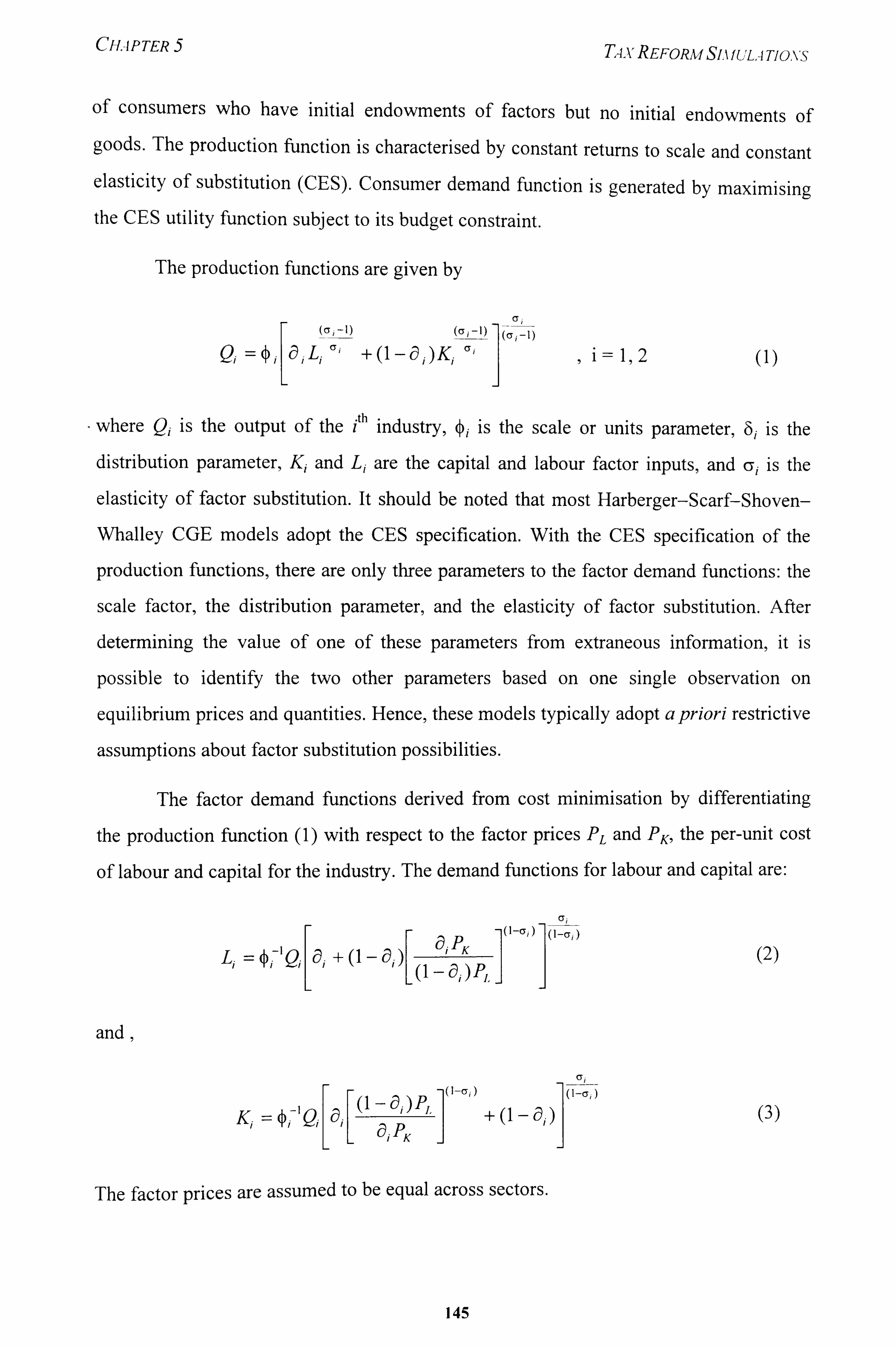
CHAPTER 5 TAx REFORM SIA f ULA TIONS

of consumers who have initial endowments of factors but no initial endowments of goods. The production function is characterised by constant returns to scale and constant elasticity of substitution (CES). Consumer demand function is generated by maximising the CES utility function subject to its budget constraint.

The production functions are given by

(cr

Qj ai Li + (I - a, )K,

where Qj is the output of the ith industry, ýj is the scale or units parameter, 6i is the distribution parameter, Ki and Li are the capital and labour factor inputs, and Gi is the

elasticity of factor substitution. It should be noted that most Harberger-Scarf-Shoven-

Whalley CGE models adopt the CES specification. With the CES specification of the

production functions, there are only three parameters to the factor demand functions: the

scale factor, the distribution parameter, and the elasticity of factor substitution. After

determining the value of one of these parameters from extraneous information, it is

possible to identify the two other parameters based on one single observation on

equilibrium prices and quantities. Hence, these models typically adopt a priori restrictive

assumptions about factor substitution possibilities.

The factor demand functions derived from cost minimisation by differentiating

the production function (1) with respect to the factor prices PL and PK, the per-unit cost

of labour and capital for the industry. The demand functions for labour and capital are:

(Yj

Li = ýj-'Qj ai + (I - ai) ai PK

_-

(I-Ci) (2)

[(I

- ai)pl, --

and ,

- Gi

Ki = ýi-'Qj ai (I - ai)PI,

ai) (1-aj I

ai PK

The factor prices are assumed to be equal across sectors.

145

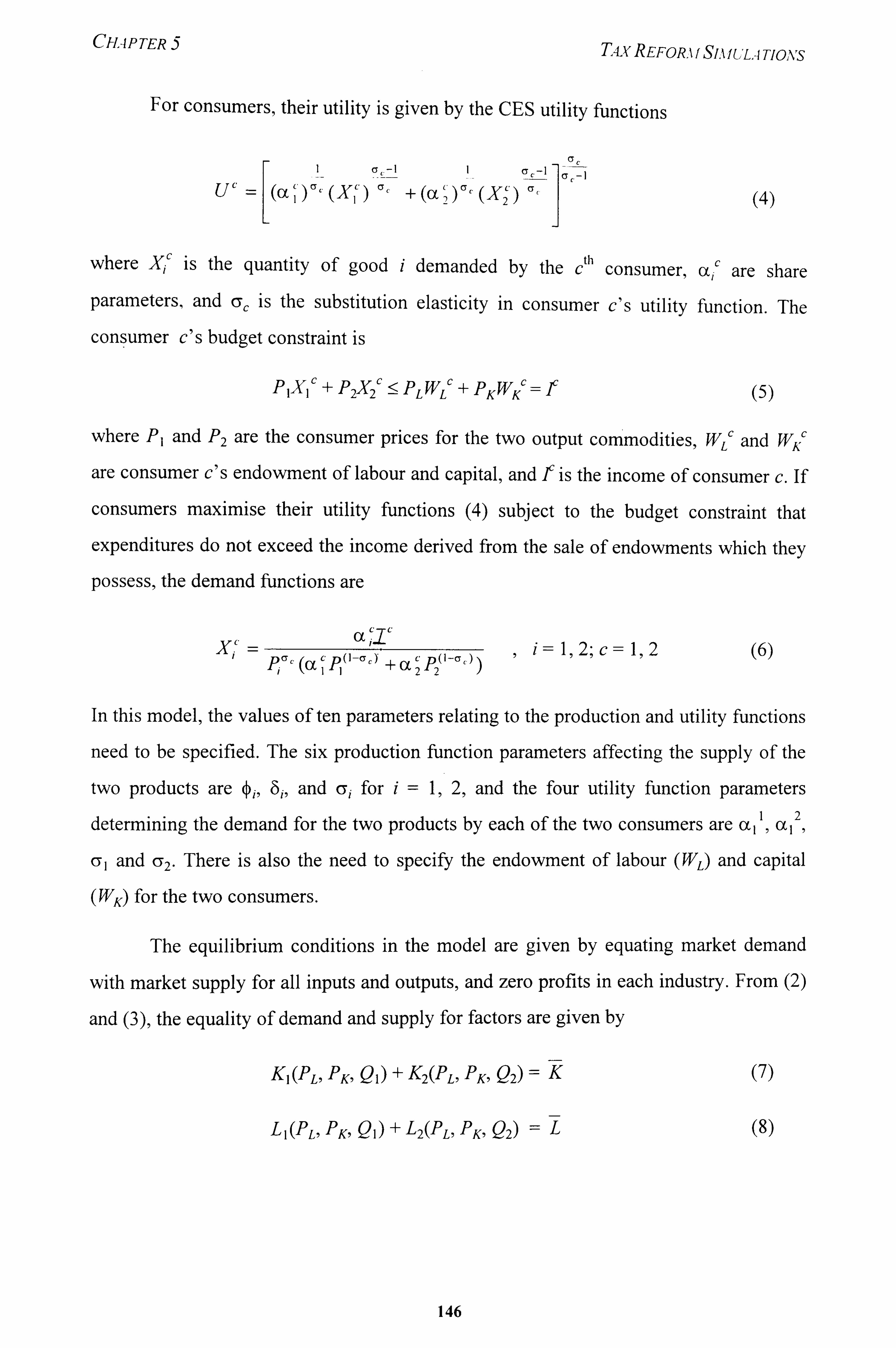
CHAP TER TIV REFOR. 1 f SIA f UL4 TIOAS

For consumers, their utility is given by the CES utility functions

cr CF

CY uc (cc c) crc (XI C+x'. )" 122

where Xj' is the quantity of good i demanded by the c"' consumer, occ are share

parameters, and cyc is the substitution elasticIty in consumer c's utility functlon. The

consumer c's budget constraint is

-cc PIXI +P2X2 "'PLWLC+PKWKC---ý-Ic (5)

where P, and P2 are the consumer prices for the two output commodities, WL' and WK'

are consumer c's endowment of labour and capital, and Ic is the income of consumer c. If

consumers maximise their utility functions (4) subject to the budget constraint that

expenditures do not exceed the income derived from the sale of endowments which they

possess, the demand functions are

a( c xi. - crc( cp(]-a, y cp (1 -CF,. ) lý 2, c=1,2 pi (X ,,

+(X2 2

In this model, the values of ten parameters relating to the production and utility functions

need to be specified. The six production function parameters affecting the supply of the

two products are ýj, 8j, and cyi for i=1,2, and the four utility function parameters

determining the demand for the two products by each of the two consumers are ot, I, (XI 2,

cy 1 and C72. There is also the need to specify the endowment of labour (WL) and capital (WK) for the two consumers.

The equilibrium conditions in the model are given by equating market demand

with market supply for all inputs and outputs, and zero profits in each industry. From (2)

and (3), the equality of demand and supply for factors are given by

KIWLý PKý Ql) + KAPLý PKý Q2) =K

LI (PLý PKqQj) + LAPL) PK5 Q2) =L

(7)

(8)

146

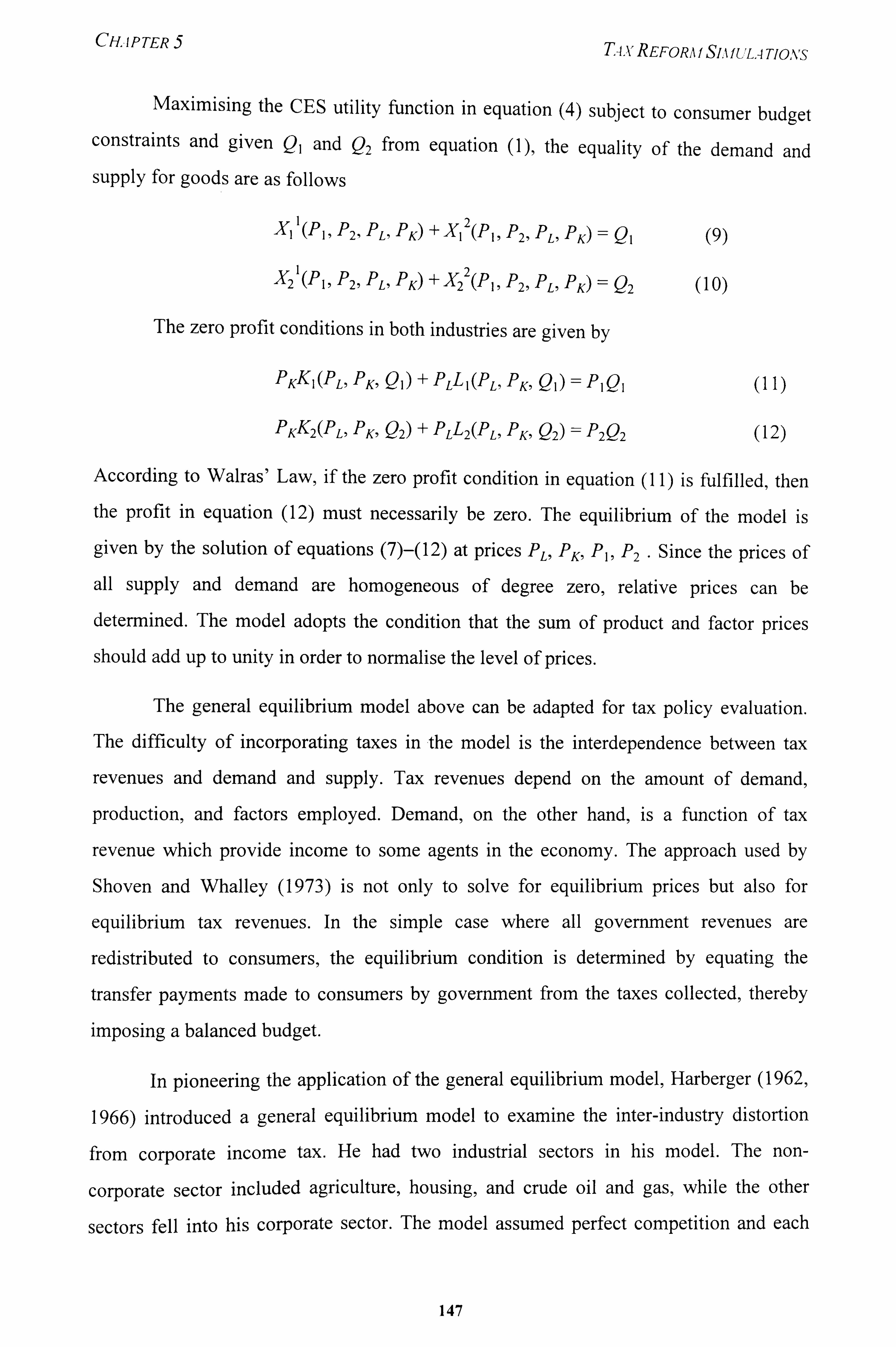
CH. IPTER TA. -V REFORA f SLI f ULA TIONS

Maximising the CES utility function in equation (4) subject to consumer budget constraints and given Q, and Q2 from equation (1), the equality of the demand and supply for goods are as follows

X, (PI P2, PLý PK) + XI 2 (PI3 P2-) PL, PK): '-- Ql (9)

+X 2(pl, X2 (p I P21 Pb PK) 2 P21 PL, PK): -- Q2 (10)

The zero profit conditions in both industries are given by

PKKI (PL5 PKý Ql) + PLL I (PL, Pký Ql): -- PI Q1 (11)

PKK2(Pb PK!, Q2) + PLL2(Pb PK1, Q2) = P2Q2

According to Walras' Law, if the zero profit condition in equation (11) is fulfilled, then

the profit in equation (12) must necessarily be zero. The equilibrium of the model is

given by the solution of equations (7)-(12) at prices PL, PKý P, 5 P2 . Since the prices of

all supply and demand are homogeneous of degree zero, relative prices can be

determined. The model adopts the condition that the sum of product and factor prices

should add up to unity in order to normalise the level of prices.

The general equilibrium model above can be adapted for tax policy evaluation. The difficulty of incorporating taxes in the model is the interdependence between tax

revenues and demand and supply. Tax revenues depend on the amount of demand,

production, and factors employed. Demand, on the other hand, is a function of tax

revenue which provide income to some agents in the economy. The approach used by

Shoven and Whalley (1973) is not only to solve for equilibrium prices but also for

equilibrium tax revenues. In the simple case where all government revenues are

redistributed to consumers, the equilibrium condition is determined by equating the

transfer payments made to consumers by government from the taxes collected, thereby

imposing a balanced budget.

In pioneering the application of the general equilibrium model, Harberger (1962,

1966) introduced a general equilibrium model to examine the inter-industry distortion

from corporate income tax. He had two industrial sectors in his model. The non-

corporate sector included agriculture, housing, and crude oil and gas, while the other

sectors fell into his corporate sector. The model assumed perfect competition and each

147

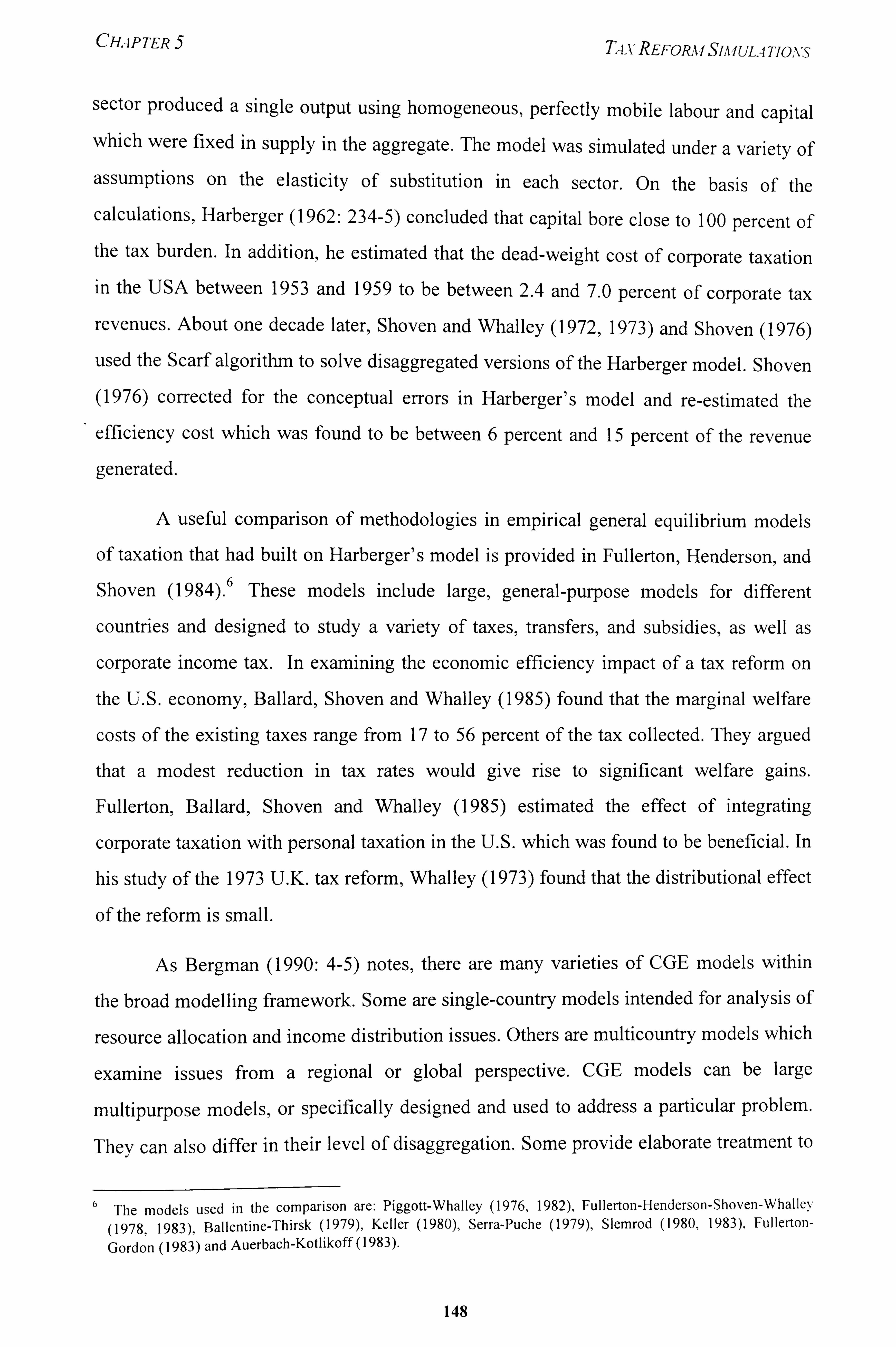
CHAPTER 5 T-ix REFORM SIAIULA TIOA'S

sector produced a single output using homogeneous, perfectly mobile labour and capital which were fixed in supply in the aggregate. The model was simulated under a variety of assumptions on the elasticity of substitution in each sector. On the basis of the

calculations, Harberger (1962: 234-5) concluded that capital bore close to 100 percent of the tax burden. In addition, he estimated that the dead-weight cost of corporate taxation

in the USA between 1953 and 1959 to be between 2.4 and 7.0 percent of corporate tax

revenues. About one decade later, Shoven and Whalley (1972,1973) and Shoven (1976)

used the Scarf algorithm to solve disaggregated versions of the Harberger model. Shoven

(1976) corrected for the conceptual errors in Harberger's model and re-estimated the

efficiency cost which was found to be between 6 percent and 15 percent of the revenue

generated.

A useful comparison of methodologies in empirical general equilibrium models

of taxation that had built on Harberger's model is provided in Fullerton, Henderson, and Shoven (1984). 6 These models include large, general-purpose models for different

countries and designed to study a variety of taxes, transfers, and subsidies, as well as

corporate income tax. In examining the economic efficiency impact of a tax reform on

the U. S. economy, Ballard, Shoven and Whalley (1985) found that the marginal welfare

costs of the existing taxes range from 17 to 56 percent of the tax collected. They argued

that a modest reduction in tax rates would give rise to significant welfare gains.

Fullerton, Ballard, Shoven and Whalley (1985) estimated the effect of integrating

corporate taxation with personal taxation in the U. S. which was found to be beneficial. In

his study of the 1973 U. K. tax reform, Whalley (1973) found that the distributional effect

of the reform is small.

As Bergman (1990: 4-5) notes, there are many varieties of CGE models within

the broad modelling framework. Some are single-country models intended for analysis of

resource allocation and income distribution issues. Others are multicountry models which

examine issues from a regional or global perspective. CGE models can be large

multipurpose models, or specifically designed and used to address a particular problem.

They can also differ in their level of disaggregation. Some provide elaborate treatment to

The models used in the comparison are: Piggott-Whalley (1976,1982), Fullerton-Henderson-Shoven-Whalleý,

(1978,1983), Ballentine-Thirsk (1979), Keller (1980), Serra-Puche (1979), Slemrod (1980,1983), Fullerton-

Gordon (1983) and Auerbach -Kotl i koff (1983).

148

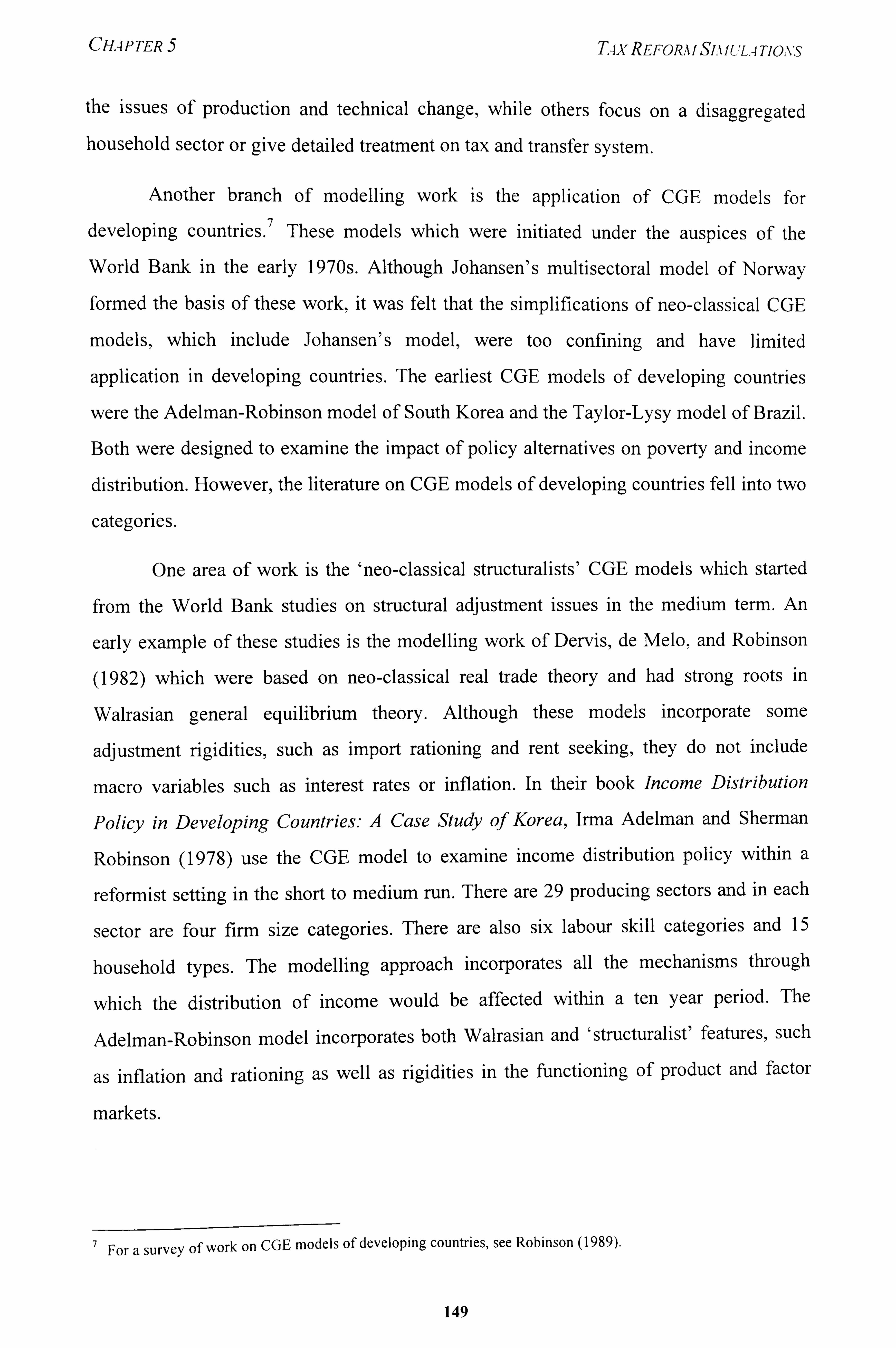
CHAPTER 5 TA. v REFORA I SIA f ULA TIONS

the issues of production and technical change, while others focus on a disaggregated

household sector or give detailed treatment on tax and transfer system.

Another branch of modelling work is the application of CGE models for

developing countries. 7 These models which were initiated under the auspi of the

World Bank in the early 1970s. Although Johansen's multisectoral model of Norway

formed the basis of these work, it was felt that the simplifications of neo-classical CGE

models, which include Johansen's model, were too confining and have limited

application in developing countries. The earliest CGE models of developing countries

were the Adelman-Robinson model of South Korea and the Taylor-Lysy model of Brazil.

Both were designed to examine the impact of policy alternatives on poverty and income

distribution. However, the literature on CGE models of developing countries fell into two

categories.

One area of work is the 'neo-classical structuralists' CGE models which started

from the World Bank studies on structural adjustment issues in the medium term. An

early example of these studies is the modelling work of Dervis, de Melo, and Robinson

(1982) which were based on neo-classical real trade theory and had strong roots in

Walrasian general equilibrium theory. Although these models incorporate some

adjustment rigidities, such as import rationing and rent seeking, they do not include

macro variables such as interest rates or inflation. In their book Income Distribution

Policy in Developing Countries: A Case Study of Korea, Irma Adelman and Sherman

Robinson (1978) use the CGE model to examine income distribution policy within a

reformist setting in the short to medium run. There are 29 producing sectors and in each

sector are four firm size categories. There are also six labour skill categories and 15

household types. The modelling approach incorporates all the mechanisms through

which the distribution of income would be affected within a ten year period. The

Adelman-Robinson model incorporates both Walrasian and 'structuralist' features, such

as inflation and rationing as well as rigidities in the functioning of product and factor

markets.

7 For a survey of work on CGE models of developing countries, see Robinson (1989).

149

CHAPTER T4. vREFORA f SIA f ULA TIOA'S

The second area of work is the 'structuralist' macro models, which are articulated by Taylor and have their roots in Marx, Kalecki, Kaldor, and Keynes (Taylor, 1983). The

'structuralist' CGE models incorporate features of macro models. For instance, Lysy and

Taylor's (1980) CGE model of Brazil uses the 'Keynesian closure' where the nominal

wage is assumed to be fixed and the aggregate price level is the macro equilibrating

variable. An increase in exogenous investment raises income and real output through the

Keynesian multiplier process and generate increased savings to match the higher level of

investment. Firms, which are assumed to be on their demand curves for labour, are

induced to hire more labour brought about by a rise in the price level which depresses

real wage. If the aggregate price level is chosen as the numeraire, then the nominal wage

serves as the equilibrating variable to achieve balance between aggregate savings and

investment. Much of the controversy on CGE models for developing countries is about

the macro 'closure' of the economy-wide models. 8 Both the Adelman-Robinson model

and the Taylor-Lysy model contain a number of macro variables and endogenised the

aggregate price level.

More recently, with the interest on the impact of macro stabilisation and

structural adjustment packages proposed by the International Monetary Fund and World

Bank for many developing countries, there has been some effort to integrate macro

models with neo-classical, trade-focused CGE models. The novel feature of these models

is the combination of macro and micro elements in general equilibrium. The paper by

Bourguignon, de Melo and Suwa (1991) introduces the general structure of the 'micro-

macro 5 economy-wide simulation model used in several case studies to assess the impact

of adjustment policies on income distribution in a number of countries, such as COte

d'Ivoire, Ecuador, Indonesia, Malaysia and Morocco. The study for Malaysia was

undertaken by Demery and Demery (1991), who used the CGE model to examine

poverty and macroeconomic policy issues.

8 See Robinson ( 199 1) for a good discussion of macro closure opt, ons In CGE models.

150

CHAPTER 5 TixREFORM SIAIULATIONS

3 EcONOMIC MODELS OF MALAYSIA

3.1 EPUModels

There are three category of economic models in used at the Economic Planning Unit (EPU) of the Prime Minister's Department in Malaysia. Among the earliest economic

models developed at EPU was the Gulbranson econometric model in 1982 to assist in

forecasting activities. This model was highly aggregated and parameterised on annual time series data for Malaysia. It was built around a set of macroeconomic income-

expenditure identities and specified along standard Keynesian lines with exogenous demands acting as the principal forcing variables in the model.

The second modelling approach is the input-output and related modelling, which includes social accounting matrices. The Malaysian input-output accounts for 1972,

1978,5 1983 and 1987 were prepared by the Department of Statistics. Using the available

input-output accounts, Pyatt and Round (1978) and Demery and Harrigan (1985a)

prepared the SAMs for 1972, while Demery and Harrigan (1990) prepared the SAM for

1983. The most sophisticated and best documented input-output planning model for

Malaysia was developed as part of the technical input for the Malaysian Industrial Master

Plan (UNIDO, 1985). The model is a dynamic input-output model which links capital

investment endogenously to output through 'accelerator' relationships where net

investment is related to the anticipated or current change in the level of output. This

model was subsequently updated using the 1983 input-output accounts to produce

projections for the revised Industrial Master Plan (UNIDO, 1992).

Regarding the third modelling approach, several CGE models have been

developed for Malaysia at EPU. The earliest CGE model was by Bakar Karim and Frank

Lysy in 1980 that was parameterised on the Pyatt and Round (1978) SAM for 1972. This

model is highly aggregated in both the goods and factor markets and provides a set of

closure options, where the analyst is able to choose alternative macroeconomic

identification restrictions. This model has not been revised, updated or used for planning

work but it does represent an important milestone in modelling at EPU. In the mid-

EPU has been involved in modelling activity for over fifteen years. Many of the models have been developed

independently to serve a variety of purpose and some are no longer in use. Harrigan (1993) provides a survey of the

EPU models on which this section is based.

151

CHAPTER 5 TAxREFORAI SlAfULATIONS

1980s, EPU commissioned a few more CGE models. The Malaysian One Sector System (MOSS), a macroeconomic model with CGE-type characteristics, was developed and described in Demery and Harrigan (1985b). MOSS contained only an aggregated production sector and commodity and one category of labour. It was based on the 1978 SAM (Demery and Harrigan, 1985a) and used principally for training purposes within EPU.

After MOSS, the General Equilibrium Model of Malaysia (GEMM) was developed as the main component of the Malaysian economic-demo graphic modelling

system at EPU. It was developed as an extension and modification of an earlier model SCORE (Demery and Harrigan, 1987) which was used to analyse the implications of

long-run population growth and demographic change in Malaysia. GEMM identified five

commodities/activities and used the classical macroeconomic closure. It was calibrated

on the 1978 SAM information although other relationships, such as those pertaining to

labour supply and fertility, were econometrically estimated using micro cross-section

data. The model assumed multi-level technologies and utilities. In production there are

separate levels for intermediate goods and value-added. At all levels in the production

hierarchy, the model assumed CES technologies. At the intermediate goods level, cost

minimisation problems were specified and solved for both domestic and imported

intermediate commodity demands. At the value-added level of production, again CES

cost minimisation was assumed, and for given levels of physical capital stock, the model

solves for labour demand. For consumption demands, a similar approach was used in the

determination of intermediate goods demands, using a mix of Stone-Geary and CES

functional forms. GEMM was subsequently extended to respond to the planning

concerns of the Unit, such as the relationship between income distribution and structural

economic adjustment.

Demery and Demery (1991) used an extended version of GEMM to assess three

counterfactual policy packages against the package chosen by the Malaysian government

in dealing with recession in the 1980s. Faced with growing fiscal deficit and widening

external debt, the government cut public expenditure, reduced interest rate, and allowed

the real exchange rate to depreciate. The simulations address the following questions:

What would have been the effect on poor households had the government gone for (a)

152

CH. Ap TER 5 T-ix REFORA f SIA f ULA TIOXS

pre-emptive adjustment and acted earlier than was actually the case; (b) milder fiscal

restraint but a bolder devaluation of the ringgit; and (c) stiffer taxes to raise revenue and

correct fiscal deficits. Demery and Demery conclude that the government had few

alternatives to restore the macroeconomic balances without making matters worse for the

poor. The government's chosen policies for cutting and switching expenditures as well as devaluing the exchange rate did much to protect the poor.

M4, the acronym for the Malaysian Micro Macro Model, is the latest CGE model

to be developed at EPU. The model, described in Demery, Harrigan, and McGregor

(1992) and Harrigan (1991), has a much richer macroeconomic texture than earlier CGE

models described above. It incorporates a number of macroeconomic closures that

encompass both Keynesian and Neo-Classical perspectives as well as a range of

alternatives in between. M4 is calibrated on the 1983 SAM and used for historical

simulations of the Malaysian economy between 1983-90. The model was subsequently

updated to 1990 and extended to address subnational and regional concerns.

An application of M4 to evaluate policy options is given in Harrigan (1996)

which examines the implications of Malaysia adopting a forest conservation policy by

surrendering the lumber value of its forest resources to non-lumber uses. Tropical forest

conservation is treated as the permanent withdrawal of an immobile resource from the

traded goods sector of a small open economy. In the lumber activity, the representative

producer is assumed to face an output constraint and seek to minimise cost. The market

for Malaysian lumber is cleared through rationing exports, while unsatisfied domestic

demand is met through imports. With lumber initially contributing 2 percent to aggregate

income, a switch from lumber to non-lumber uses of tropical forests is estimated to cost

up to 4 percent of baseline income. The associated dynamic general equilibrium

multipliers were found to be larger than unity. The study also found that prompted by the

loss of lumber foreign exchange revenue, there was a terms of trade deterioration which

accounts for about one half of the total income losses observed. This loss will

presumably be greater for countries that rely more heavily on lumber foreign exchange

revenue than Malaysia.

153

CHAPTER 5

3.2 Non-EP U Models

T4-v REFORA f SIA IUL. -j Tlo. \-S

The Malaysian Institute of Economic Research (MIER) model has been used to crenerate projections on the Malaysian macro economy as well as for policy s1mulati t: ) ions. This model, described in Semudram, Gan and Chew (1990), is essentially a neo- Keynesian macroeconometric model whereby aggregate income is demand determined. The constraints,, which are explicitly imposed on short-run movements in real activities,

are made through the commodity sector . The model is disaggregated into several blocks

comprising aggregate demand, public sector, balance of payment, monetary sector and

price block. It is highly aggregated with a total of 57 equations, of which 28 are

stochastic. As a non-CGE model,, the MIER model overlooks supply-side issues and

would not be able to accommodate issues such as labour shortages that have become

important in some sectors of the Malaysian economy.

In his Ph. D. thesis, Gan undertook an empirical study of tariff and trade policy

reform of Malaysia using an adapted version of Tower's simple linearised CGE model (Gan, 1985; Gan and Tower, 1987). Unlike the more complex non-linear CGE models,

the advantage of this model is its simplicity and flexibility. The utility functions are

assumed to be Cobb-Douglas and the model solution relied on matrix inversion and

matrix multiplication. The model used a simple 5-sector model of Malaysia with a

representative consumer and intermediate inputs used in fixed proportions in

combination with a value-added composite comprising labour, land, and capital to assess

the consequences of changed tariffs. Gan simulated two versions of the model. In the

short-run model, capital was assumed to be sector-specifiC; in the long-run model, capital

was variable, where changes in investment bring an equalisation of the after-tax rate on

investment in Malaysia with the rest of the world. The model assumed homogenous

labour and perfectly flexible wages and prices, so that resources were fully employed.

Gan found that there was a high welfare cost associated with using tariff protection to

maintain employment in import-competing sectors. The welfare cost was 91 percent of

the value of employment created at the margin in the short run and 113 percent in the

long-run. Gan also used the model to calculate shadow prices of goods, labour, and the

capital stocks in various sectors to assess the welfare implications of government

proj ects.

154

CHAPTER TAX REFORA f SIA f UL, A Tjo, vS

Barjoyai Bardai (1993) uses the Keller general equilibrium model (Keller, 1980) to evaluate the MIER 1988 proposals for tax reform in Malaysia in terms of three criteria, namely, efficiency, equity, and revenue generation. The effects of tax changes are evaluated within a static framework where two equilibrium states before and after the tax changes are compared. All relationships are assumed to be linear, implying that the

model would be better suited for examining small rather than large changes in taxes. The

model adopts the assumptions of perfect competition in the private sector markets, profit

maximisation for producers and utility maximisation for households, and equilibrium of the economic system before and after tax changes. The model does not take into account inflation, unemployment, uncertainty and growth. Compensating variation is used to

measure tax burden. In the model, there are eight classes of consumers, including foreign

and government sectors, 10 industrial groups, and 19 goods or expenditure categories.

After model calibration and construction of the data set for the benchmark

equilibrium, Bardai compared the effects of changes in the main tax categories on their

respective tax incidence. In addition, he examined the MIER tax reform proposals that

included the following: reducing corporation tax by 10 percent, introducing the value

added tax (VAT) system, increasing sales tax as a short-term measure before the

introduction of VAT, reducing export tax, and broadening the base of import tax. Bardai

argued that rather than reducing corporate tax, which is one of the most efficient and

productive tax instruments, payroll tax should be reduced instead in order to reduce the

cost of doing business in Malaysia. He favoured the introduction of VAT that was

desirable from the efficiency, equity, and tax revenue productivity criterion and would

not create inflation. He supported abolishing export taxes and proposed increasing the tax

rates on clothing and footwear and manufacturing durables.

4 DESCRIPTION OF THE MALAYSIAN MICRO-MACRO MODEL

This section presents an outline of the Malaysian Micro-Macro Model (M 4) which we

use in the tax simulations that follow. M4 is a computable general equilibrium model

belonging to the family of models described by Robinson (1991) and Bourguignon,

Branson and de Melo (1992). The model is specified for a small open economy. The

foreign sector describes both international trade in goods and services as well as trade in

155

CHAP TER 5 T. Ix REFORA f SIA f ULA TIONS

financial assets. A novel feature of M4 is providing users with an extensive menu of specification options that enable them to change parameters, behavioural assumptions, and macroeconomic identification restrictions and choose alternative characterisation of the Malaysian economy, if they so desire.

M4 encompasses macro and micro links in a general equilibrium framework. Since there are both the macro as well as the micro elements of the model, M4 is provides a rich framework for policy analysis. It is much broader than the standard open-economy IS/LM framework or the neo-classical CGE models used to analyse long-run trade and tax issues. There is much more disaggregation of the product and factor markets in M4

than the IS/LM framework; it has a financial component in addition to the real side of the

standard CGE model. M4 can be applied to focus on questions of achieving equilibrium

among various macro aggregates and the structural impact of changes in the composition

of the macro aggregates, such as savings- investment balance, balance of trade,,

government deficit, exports and imports. It also provides a good framework for analysing

changes arising from a tax reform.

As noted by Robinson (1991: 1513), there are two approaches to bringing macro features into a CGE model: (1) relationships among the macro aggregates are based on

macroeconomic theory and lie outside of the CGE model; and (2) financial variables are included in the CGE model and the notion of equilibrium is expanded to incorporate the

loanable funds market,, assets, and expectations. M4 adopts the second approach and directly incorporates macro phenomena into an operational CGE framework. It provides for an asset market closure in which the loanable funds market, with the variety of different assets, and the nominal exchange rate can be specified.

4.1 Links Between Real-Financial Economies

Although M4 shares some similar features with the financial CGE model of

Bourguignon, Branson, and de Melo (1989), there is a difference in which changes in

assets and liabilities are treated. The model by Bourguignon et. al is expressed in asset

flows based on the assumption that adjustments in asset holdings are made at the margin,

and actors are either unable or do not wish to restructure their portfolios completely for

every period. In M4 the assets are treated as stocks, and the bond or loan rates adjust to

156

CHAPTER. 5 T-ix REFORM SIMULA TIONS

clear the demand and supplies of the stocks of the assets. Stocks are given more prominence in M4 than other comparable models. In fact, one of the novel features of M'

is that transactors' balance sheet positions are modelled directly so that flows of funds

emerge in the movement from one stock position to another. Changes in asset stocks,

particularly private sector wealth, provide an important transmission mechanism from the financial to the real economies. The links between real and financial economies are

captured through endogenous interest rate changes.

Before going into the details of the model structure, it might be useful to consider the interactions between the real and financial components of the model. Since the model

is for an open economy, the balance of trade acts as a equilibrating mechanism for

achieving savings-investment balance. 10 As a system constraint, some CGE models

place the requirement that the exchange rate serves as the equilibrating variable to bring

the balance of trade into equilibrium. There is no such requirement for trade balance in

M4, and it allows for a surplus or deficit in the balance of trade. Under our assumption of

flexible exchange rate with perfect capital mobility and elastic supply of foreign capital

to the Malaysian economy, there could be unlimited capital inflows from the rest of the

world to make up for the balance of payments deficit. Changes in the flexible exchange

rate would affect aggregate savings through changes in the value of the balance of trade.

The savings-investment link is made stronger because the balance of trade, which is

endogenous in the model, adjusts to achieve equilibrium between savings and

investment.

In our model, the current account balance is endogenous. Together with other

asset yields, the nominal exchange rate adjusts to bring about the asset market

equilibrium. Changes in the real exchange rate affects the competitiveness of and

demand for exports, thereby changing the structure of production. There is also the role

of the interest rate on the real-financial interactions. The supply and demand for loanable

funds respond to changes in the interest rate. With the endogenous balance of trade

assumed in M4, the interest rate can affect investment, capital flows, the real exchange

10 The nominal system constraint for sav ings- investment is given by: SP+ SG +r-B-l =0, where SP is private

savings, SG is government savings, r is exchange rate, B is balance of trade, and I is investment.

157

CHAPTER. 5 T4, ): REFORM SLI fULA TIONS

rate, the balance of trade, which in turn influence the structure of production and employment.

4.2 Model Structure

There are eight basic transactors in the model: households, government, non- financial corporations, non-financial public enterprises, banks, Employees Provident Fund, other financial institutions,, and the rest of the world. Except for households and the rest of the world, six of the agents are institutional transactors that participate in asset markets and for whom flow and stock accounts are separately collated. M4 has thirteen

goods markets, 11 five labour markets, 12 and four asset markets. ' 3 The classification of transactors and markets is circumscribed by available data and the need for sufficient

sectoral detail for policy simulations at the macroeconomic level. M4 makes a distinction

between activities and commodities. Activities produce the goods which are sold in

commodity markets. For the factor markets, the model identifies five labour markets and three occupational groups. 14 Labour is mobile across sectors and occupations in response to wage and excess demand differentials. Physical capital is categorised into a corporate

and an unincorporated component. Capital and land are aggregated in a Hicks composite factor. They are quasi fixed, with their sectoral allocation responding to relative rewards

through the allocation of net investment. The four primary asset markets are identified by

the financial instruments. The supply and demand of these markets are equated by the

adjustment of relative yields.

As with other CGE models, the behavioural rules for the model are that Producer

are assumed to maximise profit subject to multi-level constant returns CES technology

constraints and households maximise utility subject to income constraints. These

determine input demands and output supplies. Demands that are not satisfied

domestically are made up by imports. Agents make their decisions on the basis of price

signals they observe. In the model specification adopted, we assume a perfectly

Export Agriculture, Domestic Agriculture, Forestry, Mining, Resource Manufacturing, Competitive Manufacturing,

Domestic Manufacturing, Private Services, Oil, Construction, Utilities, Government Services, and Dwellings.

12 Agricultural, Professional Non-Agricultural, Skilled Non-Agricultural, Unskilled Non-Agricultural, and Public

Sector.

13 Currency, Domestic and Foreign Equity, Loans and Deposits, and Other Domestic Assets.

14 Professional and Administrative workers, Clerical and Skilled workers, and Production and Unskilled workers.

158

CHAPTER 5 TA. v REFORA I SIA f ULA TIONS

competitive goods market and market clearing for the labour market. This means that prices are flexible and each agent is a price taker. Prices are the equilibrating variable and adjust to clear the markets for goods, factors, labour, and asset; in other words, equilibrium is achieved when all excess demands are zero, as specified in the system constraints. Markets clear in each period (one calendar year), though there are some elements of quantity adjustments in the goods markets. There are no extrinsic dynamics

in the model, other than through its adaptive treatment of expectations. Nevertheless, it

has extensive intrinsic dynamic relationships governing the accumulation of all physical

and financial stocks. Asset markets clear at the end of each period through the adjustment

of interest rates and the nominal exchange rate.

As given by the production function, agents transform labour, capital and

intermediate output into goods for the domestic and export markets. The function for

transforming output into different goods for domestic sales and export is described by the

constant elasticity of transformation. Since this is a multisectoral model, it is assumed

that goods for domestic sales and exports are different even if they share the same

sectoral classification. For the import demand function, we assume the Armington

function, that is, domestic goods sold on the domestic market are imperfect substitutes

for imports. The purchasers of goods demand a composite commodity, which is

described by a CES aggregation of imported and domestic goods. Investment demand is

exogenous for some activities, while for other it is an increasing function of Tobin's 'q',

which is the ratio of the marginal revenue product of capital to its user cost. More details

on the model structure are provided in Appendix 1.

For its solution, M4 uses the Levenberg-Marquardt algorithm which exploits the

power of both 'inverse-Hessian' and 'steepest descent' function minimisation methods.

When iterates are far from the final solution, the algorithm approximates steepest descent

and as iterates move closer to their terminal values, inverse-Hessian updates are

computed. Essentially, through a recursive ordering of the equations, variable elimination

is achieved and the model is then solved as a constrained non-linear, least squares

optimisation problem.

159

CHAP TER

4.3 Data Base and Updating

T-ix REFORM SIA fULA TIONS

The initial database for the model was the Social Accounting Matrix 1983 for Malaysia (Demery and Harrigan, 1990) which compiled the social accounts, flow of funds and asset stock data collated for the period 1983-84 into a consistent framework.

M4 was subsequently recalibrated on the more recent data with available Malaysian

National Accounts for 1990. Although the M4 database is more recent than most other Malaysian models on the economy, the original database is over a decade old. There

might be some concern that unless the data can be updated, the usefulness of this model

may be compromised. There are some options available to address this issue. The data in

the model could be updated by the user by incorporating the latest economic trends

gathered from published data in the exogenous data set, as we have done for our tax

simulations. For instance, one area of rapid change is the composition of demand,

especially the rapid increase in import and export demand starting from 1988. In

addition, the manufacturing sector expanded rapidly during the late 1980s. This was

triggered by a combination of the relaxation of controls on export-oriented

manufacturing investment, the policy of keeping the ringgit and unit labour cost low, and

deregulation of the investment policy.

The model enables other forms of 'updating' to be carried out. The technology

model accommodates various forms (Hicks, Harrod and Solow) as well as different rates

of technological progress. The improvement in labour productivity can be specified in

the model to reflect the modernisation of the economic sectors, particularly

manufacturing. The model's intrinsic dynamic relationship would also address

depreciation of the stock variables as the model moves through time.

4.4 Model Specifications

As the basic model for our tax policy reform simulations, we have adopted an

essentially neo-classical model specification, with the supply-side driving the economy.

We provide a description of the basic model assumptions below and in Table 5.1, but

more details on the specifications are provided in Appendix 2. Admittedly, many of these

160

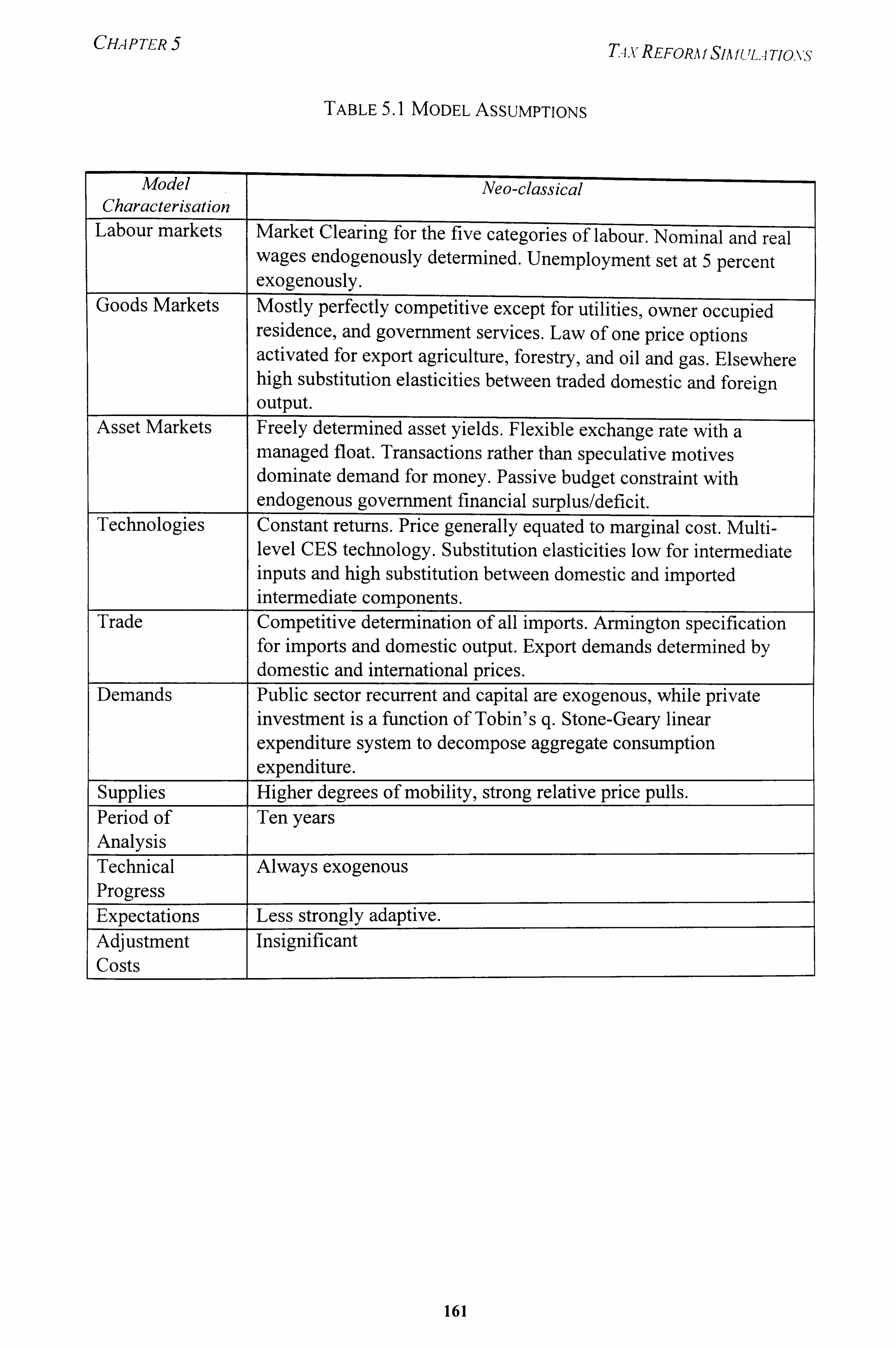
CHAPTER

TABLE 5.1 MODEL AsSUMPTIONS

T-i. v REFORA f SIA f ULA TIONS

Model Neo-classical Characterisation

Labour markets Market Clearing for the five categories of labour. Nominal and real wages endogenously determined. Unemployment set at 5 percent exogenously.

Goods Markets Mostly perfectly competitive except for utilities, owner occupied residence, and government services. Law of one price options activated for export agriculture, forestry, and oil and gas. Elsewhere high substitution elasticities between traded domestic and foreign output.

Asset Markets Freely determined asset yields. Flexible exchange rate with a managed float. Transactions rather than speculative motives dominate demand for money. Passive budget constraint with endogenous government financial surplus/deficit.

Technologies Constant returns. Price generally equated to marginal cost. Multi- level CES technology. Substitution elasticities low for intermediate inputs and high substitution between domestic and imported intermediate components.

Trade Competitive determination of all imports. Armington specification for imports and domestic output. Export demands determined by domestic and international prices.

Demands Public sector recurrent and capital are exogenous, while private investment is a function of Tobin's q. Stone-Geary linear

expenditure system to decompose aggregate consumption expenditure.

Supplies Higher degrees of mobility, strong relative price pulls. Period of Ten years Analysis Technical Always exogenous Progress Expectations Less strongly adaptive. Adjustment Insignificant Costs

161

CHAPTER 5 TAx REFORM SLI fULA TIONS

assumptions are subjective in nature, but in the absence of hard evidence such subjectivity is unavoidable. Through model calibration, we arrive at a working model that provides a fair representation of the Malaysian economy in the medium term. These assumptions appear to reflect the macroeconomic framework and objectives that are embodied in Malaysia's Second Outline Perspective Plan.

Goods markets closure. In the goods markets, we assume perfect competition for

ten goods markets, which exclude utilities, owner occupied dwellings and government

services. Utilities is based on a mark-up of 1.0, which is expressed as the ratio of the basic price of activity output (exclusive of all taxes) to marginal cost. The household

consumption of owner occupied dwellings adjusts passively to satisfy endogenous imputed rent plus a small amount of current account expenditure attached to imputed

rent. The flow of goverm-nent services is supply driven through simple technology

relationships and exogenous employment in the government sector. In addition, world

prices are imposed on export agriculture, forestry, and oil and gas commodities. There

are also export quotas on oil and forestry products.

Labour markets closure. We assume market clearing for the five categories of labour, that is, where wage is determined by equating demand and supply of agriculture,

professional, skilled, semi-skilled, and unskilled workers. This is not an unreasonable

assumption because the period under consideration is for the medium term and published

data suggest that Malaysia is close to full employment, although some frictional

unemployment remains. The labour markets are assumed to clear in each period and

satisfy an exogenously determined equilibrium unemployment rate of 5 percent. Nominal

and real wages in each labour market are determined endogenously, while the level and

growth rate for labour supply are specified exogenously. We have not opted for an

endogenous labour supply because as will be shown in Chapter 7, the labour supply for

both males and females are inelastic and negatively related to wages, suggesting that the

labour supply curves are backward bending. Furthermore, the effect of income tax on

labour supply is negligible. For the purpose of our simulations, aggregate labour force is

assumed to grow at around 3 percent per annum, with the markets for non-agricultural

labour growing faster than agricultural labour. This pattern of labour supply growth is in

162

CHAP TER 5 TA. v REFORA f SIA f ULA TIONS

keeping with actual trends exhibited in the Malaysian economy during the eighties and early nineties.

Asset market closure. The asset market closure is treated in terms of key asset

market prices or yields, namely, the bond rate, the lending rate, and the nominal

exchange rate. The bond rate and the lending rate are assumed to be flexible so that they

adjust to clear the demand and supplies of the stocks of those assets. The nominal

exchange rate is assumed to be a flexible exchange rate regime with a managed float. For

the public sector, we assume a 'passive' budget constraint where the government's financial surplus and deficit is fully endogenous.

Expectations closure. Expectations in M4 are assumed to be formed adaptively.

Agents are assumed to revise previous periods' expectations of the nominal exchange

rate and inflationary expectations by the parameter value of 0.2. The parameters are

bound by zero and unity; the larger the parameter value, the greater would be the

influence of past forecast errors on current expectations of future prices. Since the value

of 0.2 is chosen, this means that expectations are less strongly adaptive, which is

reasonable for a neo-classical model specification.

Production. The assumptions adopted for technology are fairly standard.

Activity output is produced with a multi-level CES technology where the rates of

substitution between factors may vary at each level. We assume low substitution for

different intermediate inputs (0.25) and high substitution between domestic and import

intermediate components (0.50 and above). We also assumed low substitution (0.25)

between aggregate intermediate inputs and value-added. At the value-added level, the

elasticity of substitution between capital and labour varies across sectors. The elasticity

of substitution is assumed to be high (0.75) for agriculture, forestry and construction,

medium (0.5) for manufacturing, and low (0.25) for oil and gas, mining and utilities. The

substitution composite labour technology varies between 0.25 and 0.50 for the activities.

Trade. The nature of the demands for imports and exports are determined under

this module. Import and export demands are disaggregated by commodity. In the model,

imports are classified by intermediate, consumption and investment uses. We assume that

the competitive option is applied in the determination of all imports. This activates the

163

CHAPTER 5 T-i. vREFORA f SIMULA TIMIS

Armington specification which requires some assumptions on the substitution elasticities. Imports respond to relative prices and domestic demand. For our model, we assume that the law of one price (LOP) closure is applied to export agriculture, forestry, and oil and gas, where Malaysian producers accept world prices (in foreign currency units) when making their supply decisions. In all other activities, Malaysian producers enjoy some degree of price autonomy. For resource and traded manufacturing exports we impose

export price elasticities that are comparatively large (ý! 5), which are close to those

estimated by Reidel (1988) for Hong Kong's manufactures. Export demands are determined by domestic prices relative to the prices of similar commodities produced

elsewhere in the world.

Demand. For the demand components, public sector recurrent and capital

expenditure are exogenously determined. Private investment is a function of Tobin's q. All other demand components are taken to be endogenous to the model. Private

consumption is a function of household disposable income, but is also affected by private

sector wealth (determined by capital accumulation net of foreign indebtedness) and

interest rates.

Growth rates of sectoral output are determined endogenously for all sectors

except forestry, oil and LNG and public services. In establishing the sectoral growth

rates, we are guided by the targets set in the Second Outline Perspective Plan, 1991-2000

(Malaysia, 1991). During the decade, forestry output is assumed to exhibit constant

growth, oil and LNG production grows very slowly at 1.5 percent per annum, and public

services output grows at the economy-wide average rate of around 8 percent per annum.

For the remaining sectors of the economy, the growth trend is determined largely by the

assumed growth rates of their capital stocks (net investment) and the rate of growth of

labour augmenting technological progress. Our assumptions imply fast growth in

manufacturing (10- 15 percent) and private services (9 percent); slow growth in

agriculture in agriculture and mining (1-3 percent), and average growth (7-8 percent) in

the remaining sectors. These growth rates are not unreasonable given the track record of

sectoral growth, especially during the last few years.

The Stone-Geary linear expenditure system is used to decompose aggregate

consumption expenditures. The demands for durable and semi-durable goods are

164

CHAPTER 5 TA. v REFoRm SIA IULA TIONS

assumed to be income elastic while the demand for food and drink is income inelastic.

Other income elasticities are close to unity. The equat ions governing the split of

consumption demands into their domestic and imported components have universally high substitution elasticities. In the case of investment, the demands for capital goods by

NFPEs and the government are treated as exogenous. The demand for capital goods by

the other activities are determined endogenously. Investment demands are translated into

demands for commodities via a capital aggregation matrix and split into their domestic

and imported components using Armington relationship.

Finance. In the asset markets, interest rates and nominal effective exchange rate

are market determined. The supply of base money, foreign currency (backing money)

and bonds are set exogenously at a growth rate that imply inflation of 2-3 percent per

annum. The public sector finances its residual deficit by borrowing from foreign sources,

the supply of which is infinitely elastic at world interest rate. The nominal effective

exchange rate adjusts in each period, and together with the model's asset yields, bring

about an equilibrium in the asset market at end of period.

165

CHAPTER 5 T4xREF0PA1 SIMULA TIONS

5 MODEL CALIBRATION

The model is calibrated against actual data over the period 1990-95. Two sets of controls are used:

1. National Accounts controls for variables, such as real GDP, consumption, investment, government expenditure, exports, imports, etc.

2. Tax receipts in current prices.

The aim of this exercise is to 'mimic' as closely as possible the structure and trends of the economy. It is important to bear in mind that unlike time-series models, CGE models

such as M4 are better in projecting broad trends of economic developments rather than

short-run business cycle fluctuations. What is essential in the calibration exercise is

whether the model can produce estimates for a number of key endogenous variables that

correspond to actual outcomes.

After calibrating the model with published macroeconomic data, we arrived at the

baseline model that was used for subsequent tax reform simulations. The model

predictions and the published figures of the Economic Report are given in Table 5.2.

Generally, the model reproduces the macroeconomic developments between 1990-95

rather well, although estimates for some variables are closer to published data than

others. The annual growth rates for nominal GDP, private consumption and government

consumption generated by the model are fairly close to the published data for 1990-95.

The model's estimated growth rates are lower for total investment, exports and imports

than published data, though not unreasonably so. The base-run trajectories of nominal

GDP, consumption, investment, export and import for 1990-95 are shown in Figure 5.2.

In the second stage, we calibrated the model against the published tax receipts in

current prices for 1990-95. The following taxes are represented in the exogenous

database:

1. Domestic Taxes (intermediate uses, consumption uses, and capital uses)

2. Export Taxes

3. Import Taxes (intermediate uses, consumption uses, and capital uses)

166

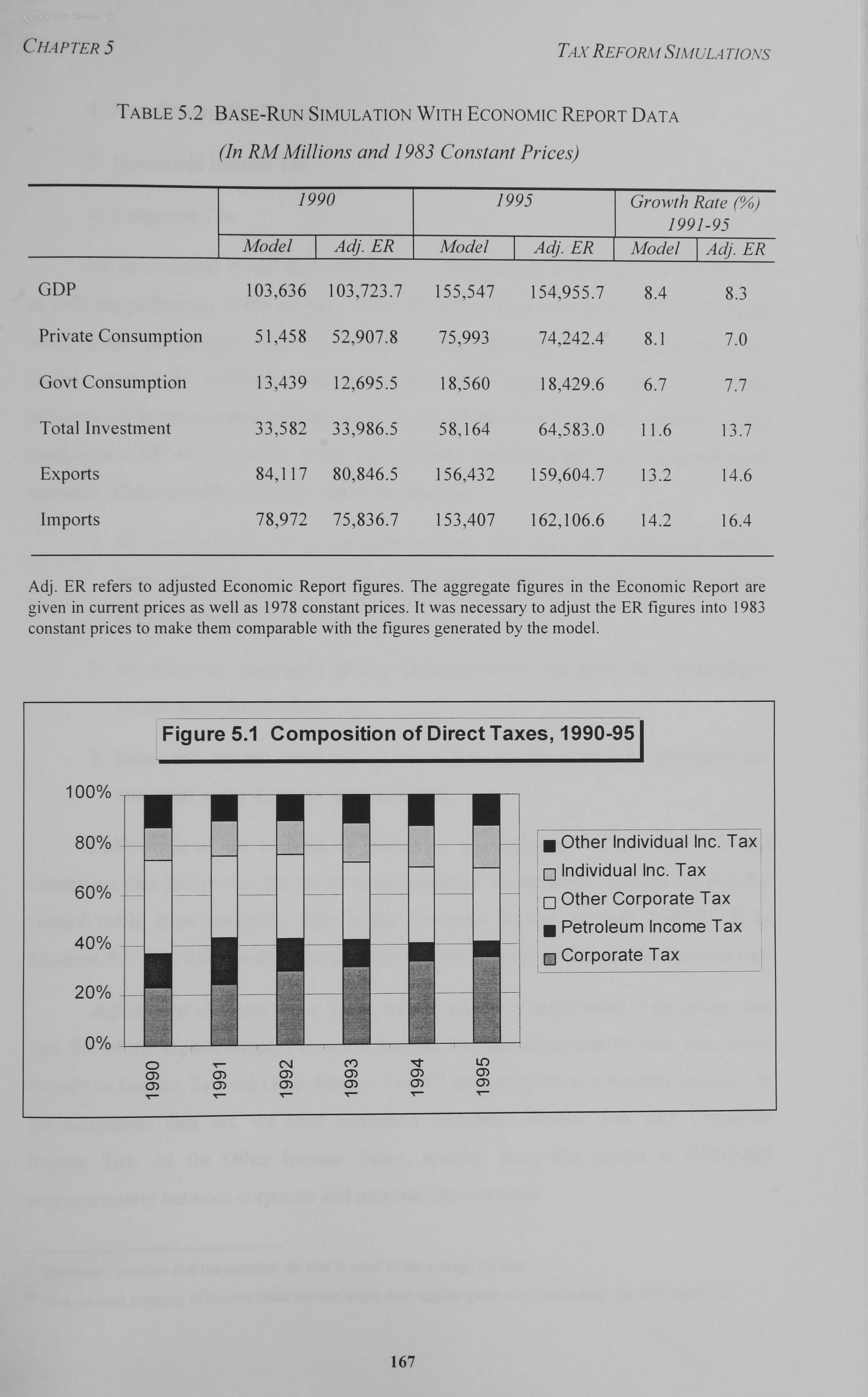
CHA P TER T, 4. v REFORA f SIA f ULA TIONS

TABLE 5.2 BASE-RuN SIMULATION WITH ECONOMIc REPORT DATA

(In RM Millions and 1983 Constant Prices)

1990 1995 Growth R"to ý'X)

GDP

Private Consumption

Govt Consumption

Total Investment

Exports

Imports

'1-9'91 -'95

Model Adj. ER Model Adj. ER Vod-e7l-T Adj. ER

103,636 103,723.7 155,547 154,955.7 8.4 8.3

51,458 52,907.8 75,993 74,242.4 8.1 7.0

13,439 12,695.5 18,560 18,429.6 6.7 7.7

33,582 33,986.5 58,164 64,583.0 11.6 1). 7

84,117 80,846.5 156,432 159,604.7 13.2 14.6

78,972 75,836.7 153,407 162,106.6 14.2 16.4

Adj. ER refers to adjusted Economic Report figures. The aggregate figures in the Economic Report are given in current prices as well as 1978 constant prices. It was necessary to adjust the ER figures into 1983 constant prices to make them comparable with the figures generated by the model.

Figure 5.1 Composition of DirectTaxes, 1990-95

100%

80%

60%

40%

20%

0%

Other Individual Inc. Tax,

Individual Inc. Tax Other Corporate Tax Petroleum Income Tax

E] Corporate Tax

167

TI- N cle) I- LO CY) 0) 0) 0) CY) 0) CY) CT) a) M Ir- Ir- T-

CHAPTER

Non-Commodity Taxes

5. Household Income Tax

6. Corporate Tax

T-Lv REFORA I SIA f (-'L. 4 Tio, \, S

M4 is a sectoral model that provides rich details about production sectors. This is an over- simplification of the complex structure of tax rates in practice, but in a micro- macro model of this type, including a highly detailed structure of taxes would make the model excessively unwieldy and undesirable. M4 treats direct taxes as simply proportional to income and indirect taxes as ad valorem taxes. Because of this, the tax categories in M4 do not always match conveniently with those published in government accounts. Three specific problems should be stressed:

1. m4 has consolidated government accounts and does not distinguish central from local or state government. This is particularly problematic since the latter has grown significantly since 1983.

2. M4 does not separately identify petroleum tax, but taxes the consolidated

corporate sector income.

3. Sales and service taxes and excise duties are not separately identified but

classified under domestic indirect taxes.

Calibration of tax revenue is performed by adjusting the tax rates' 5 in the

exogenous data file so that the tax revenues predicted by the model correspond with the

control totals from published data in the Economic Report between 1990-95. It is

assumed that for 1996 onwards, the tax rates for 1995 remain unchanged for the base run.

Adjustment of direct taxes. There are two groups of direct taxes in the exogenous

data file of the model, namely, Personal Income Tax and Corporate Income Tax. Since

Petroleum Income Tax and Other Income Taxes 16 are not given as a separate category in

the exogenous data set, we have combined Petroleum Income Tax with Corporate

Income Tax. As for Other Income Taxes, revenue from this source is distributed

proportionately between corporate and personal income taxes.

15 The model assumes that the marginal tax rate is equal to the average tax rate.

16 This residual category of income taxes include stamp duty, capital gains duty, estate duty, and film rental tax.

168

CHAPTER. 5 TAX REFoRA f SIA f ULA TIONS

In the government accounts, the revenue sources received by the Federal Government are given in some detail, but not for revenue received by the state and local governments and statutory authorities, which are given in aggregate. For data consistency, care was taken to ensure that the payments made by institutions and transactors to government agencies should be reflected on the receipt side. For modelling purpose, we treat the Own Sources of Revenue category for state and local governments and statutory authorities as tax revenues. The approach adopted was to consider these sources of revenue as dependent on the income flows of households and corporations, even though they are not levied as a proportion of these. The rationale for this approach is that the revenues received by state and local governments tend to be related to property ownership and wealth, such as land taxes and property assessment rates. These are likely

to move with income. The revenue from statutory authorities is derived from services rendered to households and firms. The demand for these services is assumed to be a function of income. The composition of actual direct taxes is shown in Figure 5.1. This

chart makes a distinction between Personal Income Tax and Corporate Tax received by

the Federal Government and the Other Personal Income Tax and Other Corporate Tax

categories that resulted from the adjustments made.

Adjustment of indirect taxes. The exogenous data file provides export duties,

import duties, domestic indirect taxes and non-commodity taxes as separate categories.

In the model, sales and service taxes, excise duties and other indirect taxes are grouped

under domestic indirect taxes because their contribution to total revenue was small in the

1983 SAM. Non-commodity taxes refer to the revenue for the Federal Government

coming from a disparate list of revenue items. They include earnings from government

commercial undertakings, interest and returns on investment, licences, service fees, road

tax, fines and forfeitures, rental revenue from Federal Territories, contributions from

foreign governments and international agencies, and petroleum royalties and gas cash

payments. This category of taxes is calculated in the model by relating them to value

added. Table 5.3 shows the base-run estimates on revenue, expenditure and budget

deficits and the control totals based on published data for 1990

169

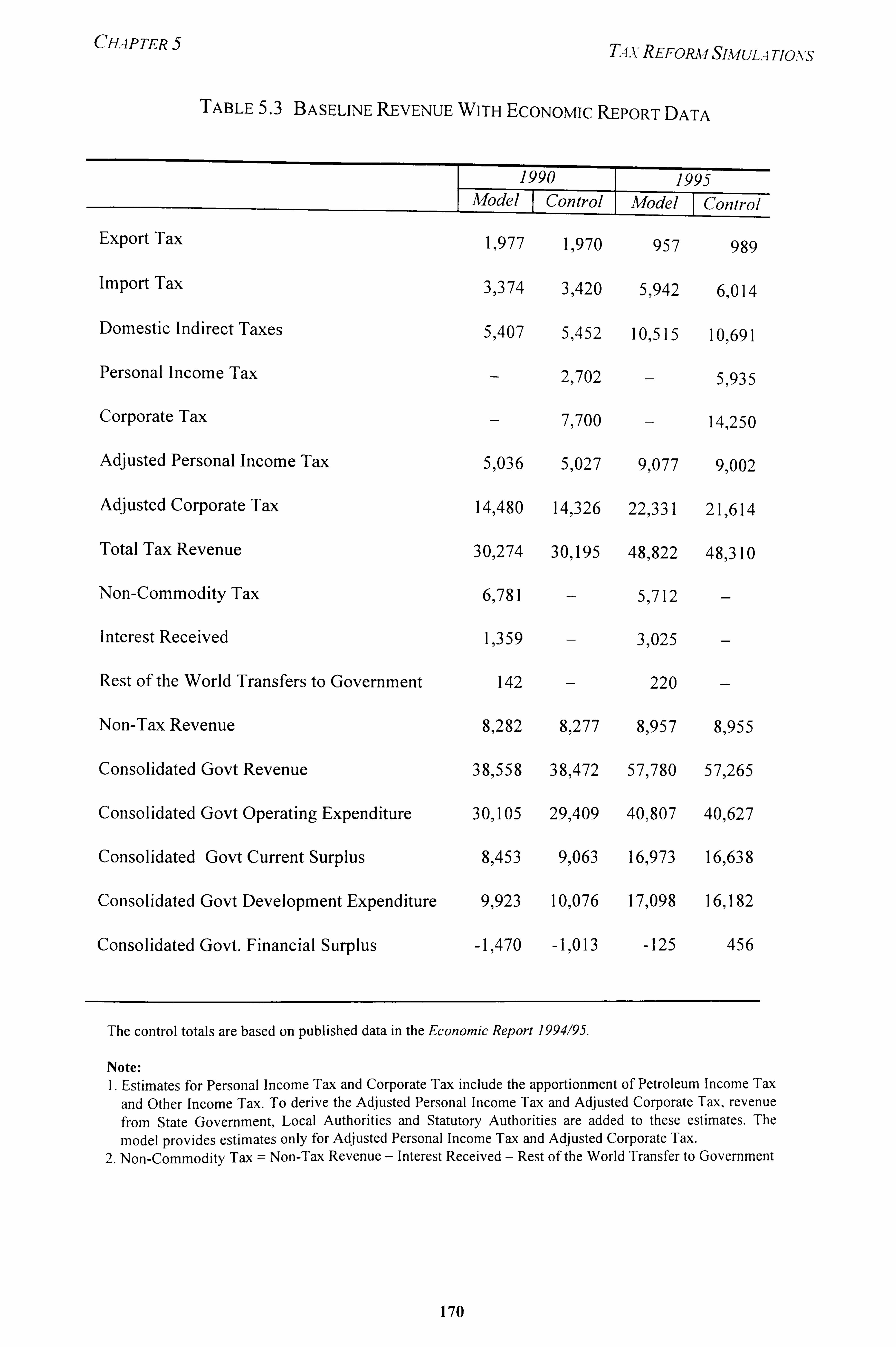
CHAPTER T-i. v REFORM SIMULA TIONS

TABLE 5.3 BASELINE REVENUE WITH ECONOMic REPORT DATA

Export Tax

Import Tax

Domestic Indirect Taxes

Personal Income Tax

Corporate Tax

Adjusted Personal Income Tax

Adjusted Corporate Tax

Total Tax Revenue

Non-Commodity Tax

Interest Received

Rest of the World Transfers to Government

Non-Tax Revenue

Consolidated Govt Revenue

Consolidated Govt Operating Expenditure

Consolidated Govt Current Surplus

Consolidated Govt Development Expenditure

Consolidated Govt. Financial Surplus

1990 1995 Model ý Control Model I Control

1,977 1,970 957 989

35374 31420 5,942 6,014

5,407 5,452 10,515 10,691

- 2ý702 - 55935

- 7,700 - 14,250

55036 55027 9,077 9,002

149480 14,326 22ý331 21,614

30,274 30,195 48,822 48,310

61781 - 5,712 -

11,359 31,025

142 - 220 -

8ý282 81277 8,957 8,955

389558 38,472 57,780 575265

30,105 29,409 40,807 40,627

8,453 91063 16ý973 16,638

9ý923 10,076 17ý098 16,182

-1,470 -11013 -125 456

The control totals are based on published data in the Economic Report 1994195

Note: 1. Estimates for Personal Income Tax and Corporate Tax include the apportionment of Petroleum Income Tax

and Other Income Tax. To derive the Adjusted Personal Income Tax and Adjusted Corporate Tax, revenue from State Government, Local Authorities and Statutory Authorities are added to these estimates. The

model provides estimates only for Adjusted Personal Income Tax and Adjusted Corporate Tax. 2. Non-Commodity Tax = Non-Tax Revenue - Interest Received - Rest of the World Transfer to Government

170

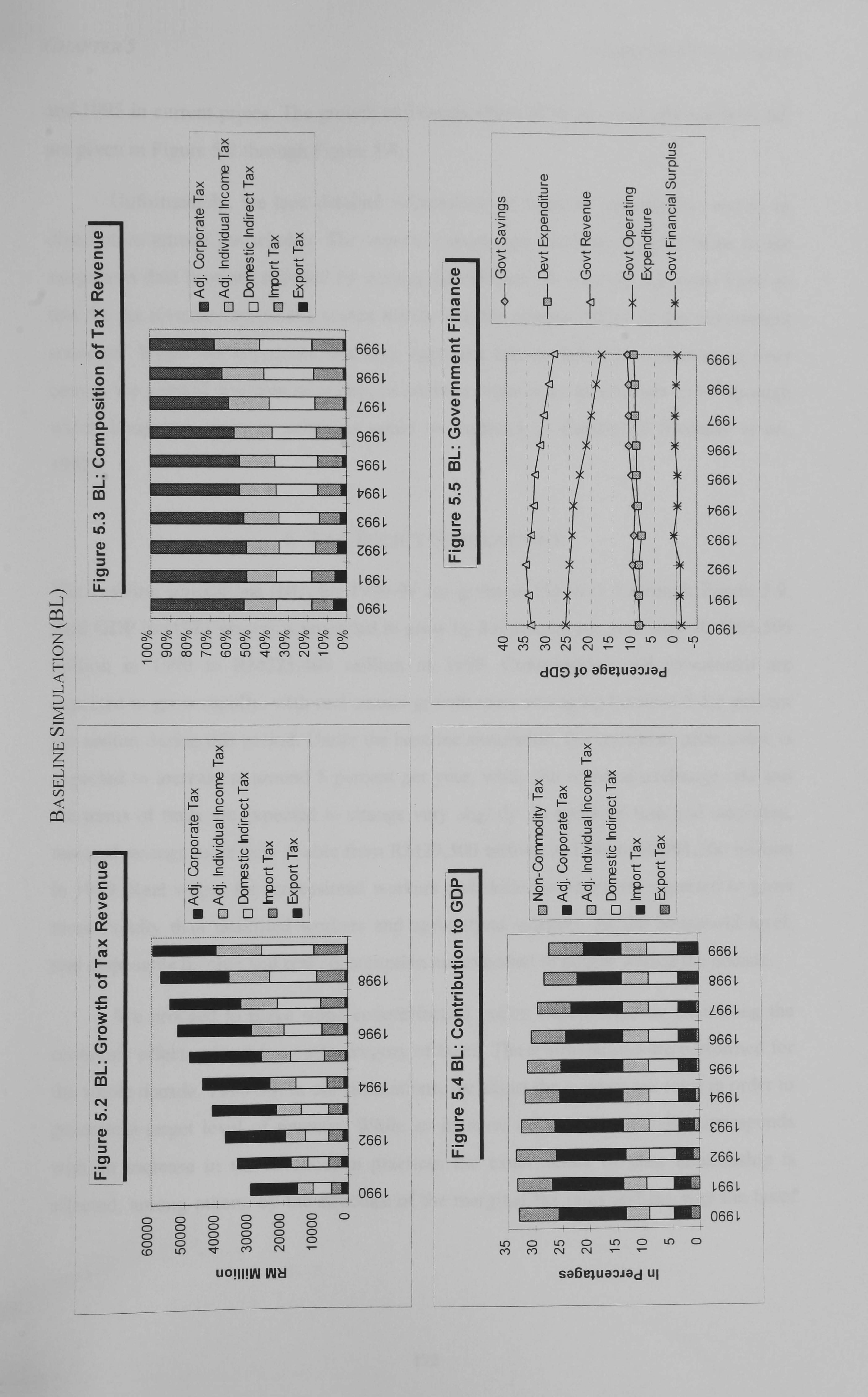
LL)

(D w

x

0 c 0

0 M E 0 L) *i m m ui

x

0

0

04 L6

U-

x m x

x

(D

0

(D

0

_0 <

m

>

_0 <

C) 0

X m

F-

0

ý

X

0 a-

Lý 0 0 ED D 0

x cu

ca (D _Z6 10

o x x CL >

o C/) 8

-9 0 0 . -.:, _0 . -L. _0

CL

< < 11 El 0

666 ý

966 ý

Z66 ý

966 ý

966 ý

V661

C66 ý

Z66 ý LL ý66ý

066 ý

0-

vi 0)

Q) =3

_0 :3

CY)

. EZ U)

m CL

(1) 0- : t: ý c

m c

oC : a) - 0 0 (D > C)- (OD Lý

5 (OD

CL

1 10

ia

966

a 0

966 L L)

t, 66 L t6

Z66 L

066 ý

x

x 0

I1

co " o

0-

(3 <

IV :3

-9 .>

<

-0 c

- L)

U) rs

x

g 0 k

x

ý('o

0 Lý

0 El 0 m m

-ö0- C-5-0 -. 2- Jc> C-iO- -. 2 -. o- 1.2 C-501 ä12 I-: ýo CD CD CD CD CD CD CD CD CD CD CD CD CY) 00 f, - (D Lf) X: r n C', J

C: ) CD C: ) CD CD C: ) CD CD CD CD CD CD CD

CD CD CD CD C: ) CD CD CD (D CD CD CD

(0 U') (Y) cli

UOIII! W Wu

CHAPTER 5 T4. v REFORNI SIA fUL, 4 TJOAS

and 1995 in current prices. The growth and composition of tax revenue generated by M4 are given in Figure 5.2 through Figure 5-4.

Unfortunately, we lack detailed information on taxes by commodity, sector, or distribution among households. The import, export, and domestic indirect taxes in the

exogenous data base are adjusted by scaling the relevant tax rates on a pro-rata basis so that the tax revenues from each source match with the revenue tables of the government

accounts. While we appreciate that this approach has an inherent weakness, it does

convey the general direction of policy. In addition, there is no mechanism in M4 through

which lump-sum taxes or subsidies could be imposed or distributed (Demery et al., 1992).

6 TAX POLICY SIMULATIONS

The baseline simulations (BL) for 1990-99 are given in Figure 5.5 through Figure 5.9.

Real GDP in (1983 prices) is projected to grow by 8.6 percent per year from RM106,500

million in 1990 to RM225,400 million in 1999. Consumption and investment are

expected to grow rapidly, with real annual growth rates averaging between 8-8.5 percent

per annum. during this period. Under the baseline simulation, the consumer price index is

expected to increase at around 5 percent per year, while the nominal exchange rate and

the terms of trade are expected to change very slightly. In terms of financial surpluses,

national savings more than double from RM29,500 million in 1990 to RM91,300 million

in 1999. Real wages for professional workers and skilled workers are expected to grow

more rapidly than unskilled workers and agricultural workers. At the household level,

real disposable income and real consumption are expected to double during the decade.

We proceed to make some counterfactual policy experiments by examining the

economic effects of varying each category of taxes. These simulations are performed for

the whole decade, 1990-99. In our simulations, we adjust the average tax rates in order to

generate a target level of revenue. While an increase in tax rate generally corresponds

with an increase in tax revenue, in practices the exact nature of their relationship is

affected, among others, by the structure of the marginal tax rates and the way the taxes

172

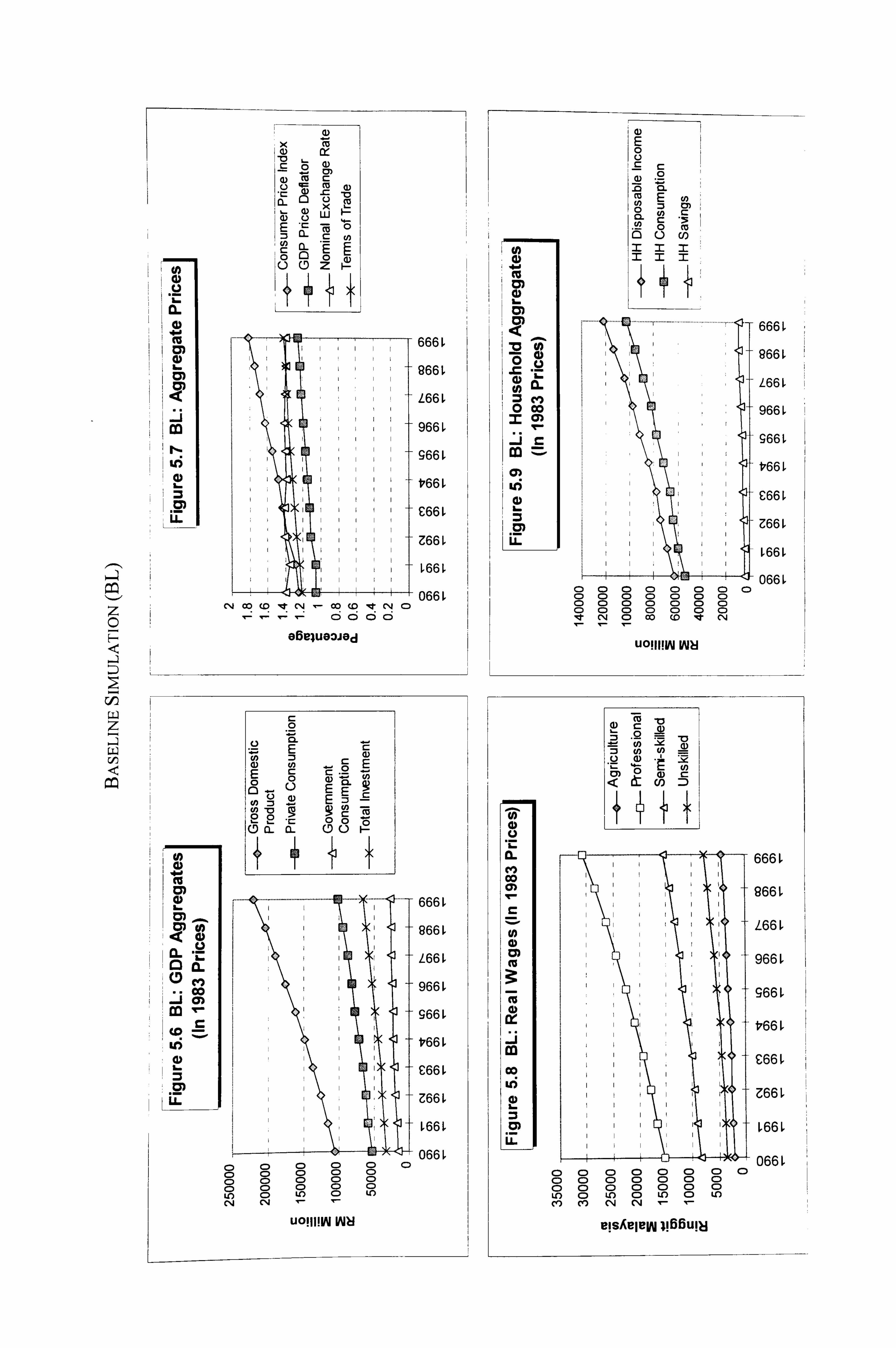
z C H

rID

z LL CIV)

CL

U)

ý ED

x UJ ýE

-c-- -E 0 :3 12- C cn

0 Z

c 0

E

E 0 c- ; - 0 . - (L) CL E E E ý

(D CL r_ CL

0 0

co (7)

a

L6

E 0 C c 2 . m E co 0 0 CL c co o m C/5 1: Z: -r

. ............ .................................... ......... .- 666L

966L

L66L

966L

966 L

V66 L

C66 L

Z66 L

66L

066 L 0 C) C) 0 0 C) 0 C) 0 C) 0 C) C) 0 0 C) 000 C) 00 a C) 't CN 0 co (D Ict

UOIII! W WN

,a (D

CL m co

co

tm E

cm 0 a) r_

666 ý

966 L

L66 ý

966 L

966 L

t, 661

Z66 L

066 L 0 C C) C) 00 C) C) C

) CD C) C) C) C) CD ) 0 Ul 0000 C) CD

C) Ul C) Ul CD Ul CO cn CN CN V-- T-

leisAeloW I! r)Buil: i

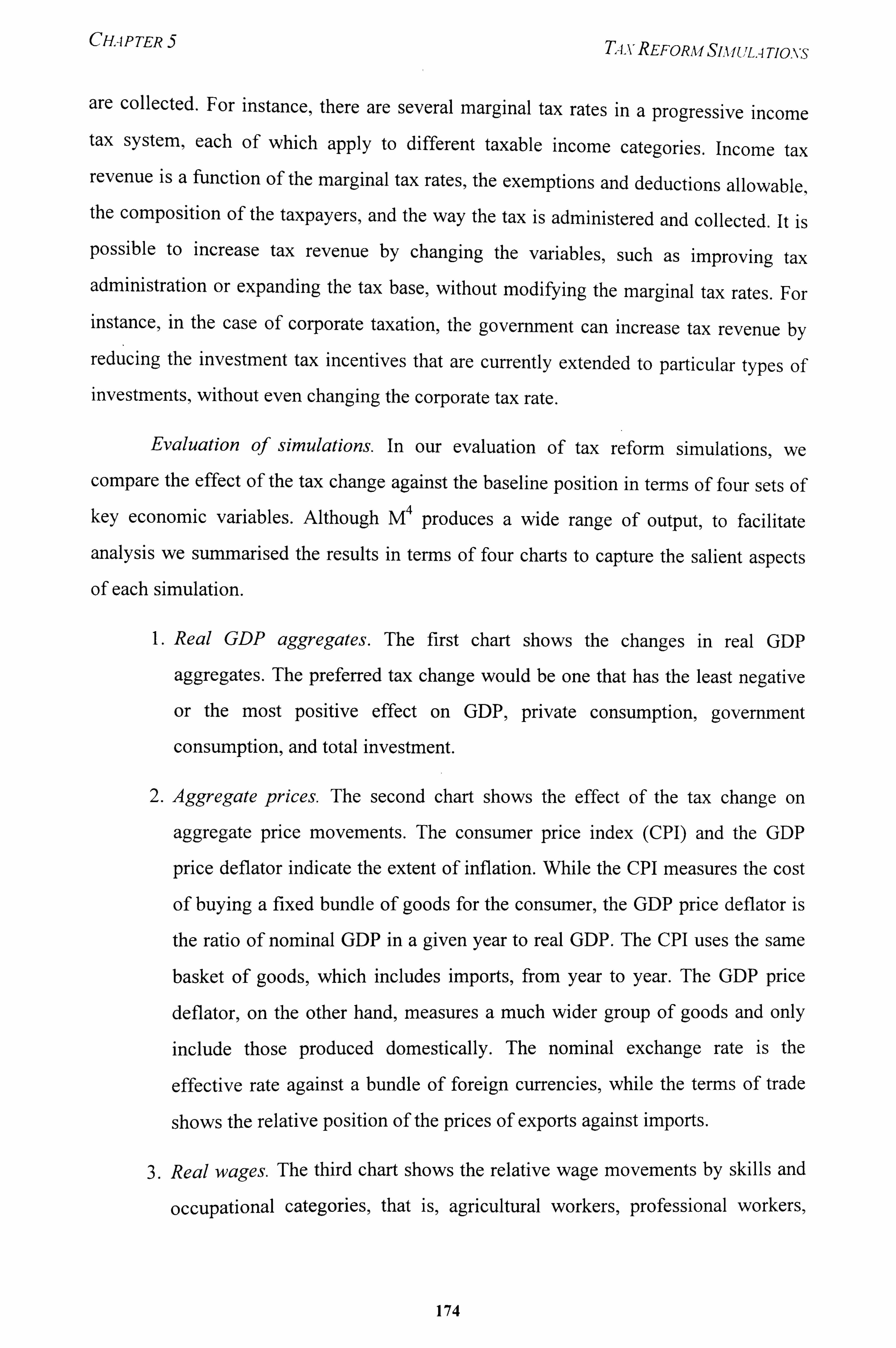
CHAPTER 5 TIV REFORM SIA f ULA TIONS

are collected. For instance, there are several marginal tax rates in a progressive income tax system, each of which apply to different taxable income categories. Income tax revenue is a function of the marginal tax rates, the exemptions and deductions allowable, the composition of the taxpayers, and the way the tax is administered and collected. It is

possible to increase tax revenue by changing the variables, such as improving tax administration or expanding the tax base, without modifying the marginal tax rates. For instance, in the case of corporate taxation, the government can increase tax revenue by

reducing the investment tax incentives that are currently extended to particular types of investments,, without even changing the corporate tax rate.

Evaluation of simulations. In our evaluation of tax reform simulations, we

compare the effect of the tax change against the baseline position in terms of four sets of key economic variables. Although M4 produces a wide range of output, to facilitate

analysis we summarised the results in terms of four charts to capture the salient aspects

of each simulation.

1. Real GDP aggregates. The first chart shows the changes in real GDP

aggregates. The preferred tax change would be one that has the least negative

or the most positive effect on GDP, private consumption, government

consumption, and total investment.

2. Aggregate prices. The second chart shows the effect of the tax change on

aggregate price movements. The consumer price index (CPI) and the GDP

price deflator indicate the extent of inflation. While the CRI measures the cost

of buying a fixed bundle of goods for the consumer, the GDP price deflator is

the ratio of nominal GDP in a given year to real GDP. The CPI uses the same

basket of goods, which includes imports, from year to year. The GDP price

deflator, on the other hand, measures a much wider group of goods and only

include those produced domestically. The nominal exchange rate is the

effective rate against a bundle of foreign currencies, while the terms of trade

shows the relative position of the prices of exports against imports.

3. Real wages. The third chart shows the relative wage movements by skills and

occupational categories, that is, agricultural workers, professional workers,

174

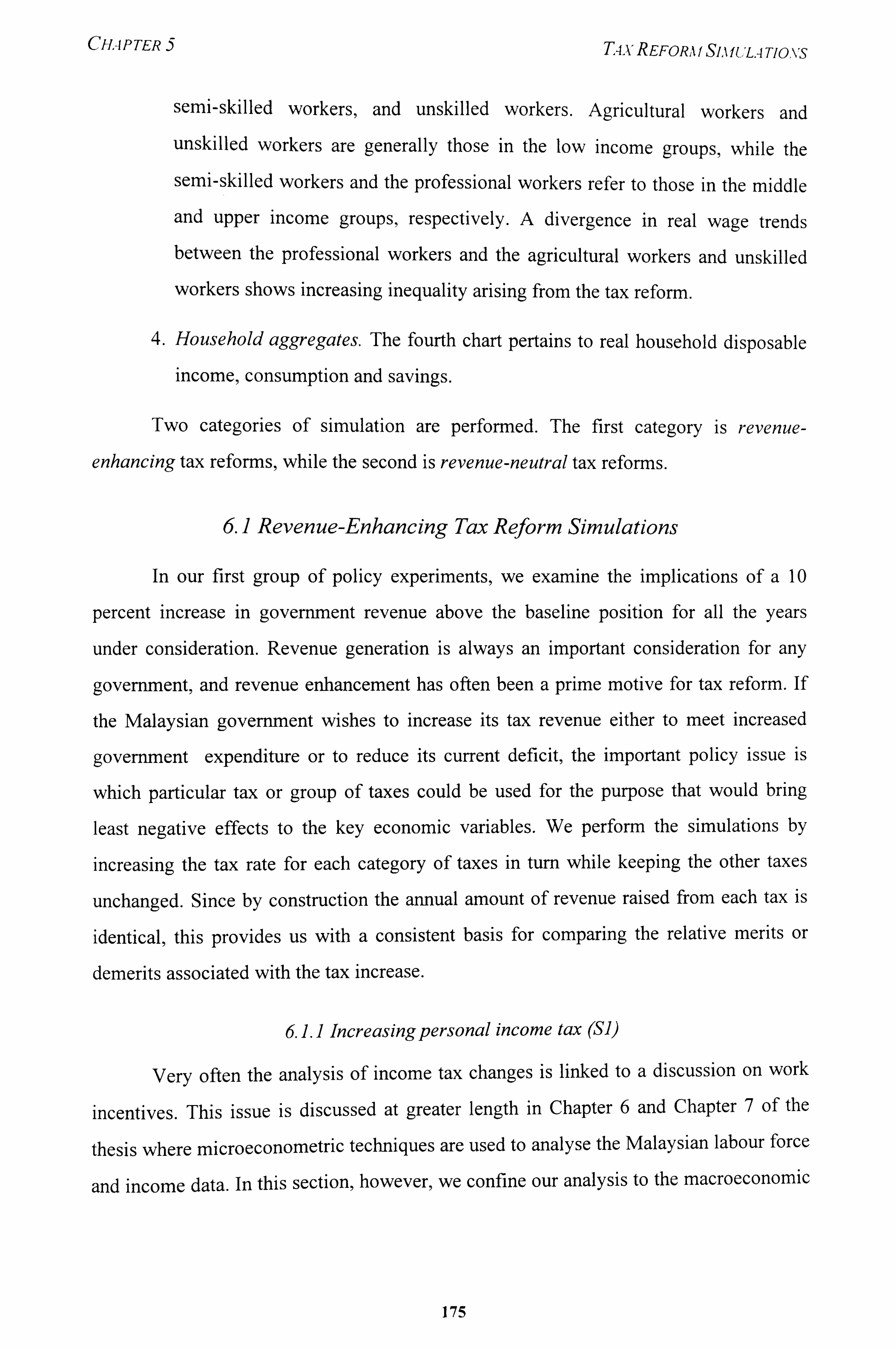
CHAP TER T4x REFORA f SIA fULA TIONS

semi-skilled workers, and unskilled workers. Agricultural workers and unskilled workers are generally those in the low income groups, while the

semi-skilled workers and the professional workers refer to those in the middle and upper income groups, respectively. A divergence in real wage trends between the professional workers and the agricultural workers and unskilled workers shows increasing inequality arising from the tax reform.

4. Household aggregates. The fourth chart pertains to real household disposable

income, consumption and savings.

Two categories of simulation are performed. The first category is revenue-

enhancing tax reforms, while the second is revenue-neutral tax reforms.

6.1 Revenue-Enhancing Tax Reform Simulations

In our first group of policy experiments, we examine the implications of a 10

percent increase in govenu-nent revenue above the baseline position for all the years

under consideration. Revenue generation is always an important consideration for any

government, and revenue enhancement has often been a prime motive for tax reform. If

the Malaysian goverm-nent wishes to increase its tax revenue either to meet increased

govenu-nent expenditure or to reduce its current deficit, the important policy issue is

which particular tax or group of taxes could be used for the purpose that would bring

least negative effects to the key economic variables. We perform the simulations by

increasing the tax rate for each category of taxes in turn while keeping the other taxes

unchanged. Since by construction the annual amount of revenue raised from each tax is

identical, this provides us with a consistent basis for comparing the relative merits or

demerits associated with the tax increase.

6 LI Increasing personal income tax (SI)

Very often the analysis of income tax changes is linked to a discussion on work

incentives. This issue is discussed at greater length in Chapter 6 and Chapter 7 of the

thesis where microeconometric techniques are used to analyse the Malaysian labour force

and income data. In this section, however, we confine our analysis to the macroeconomic

175

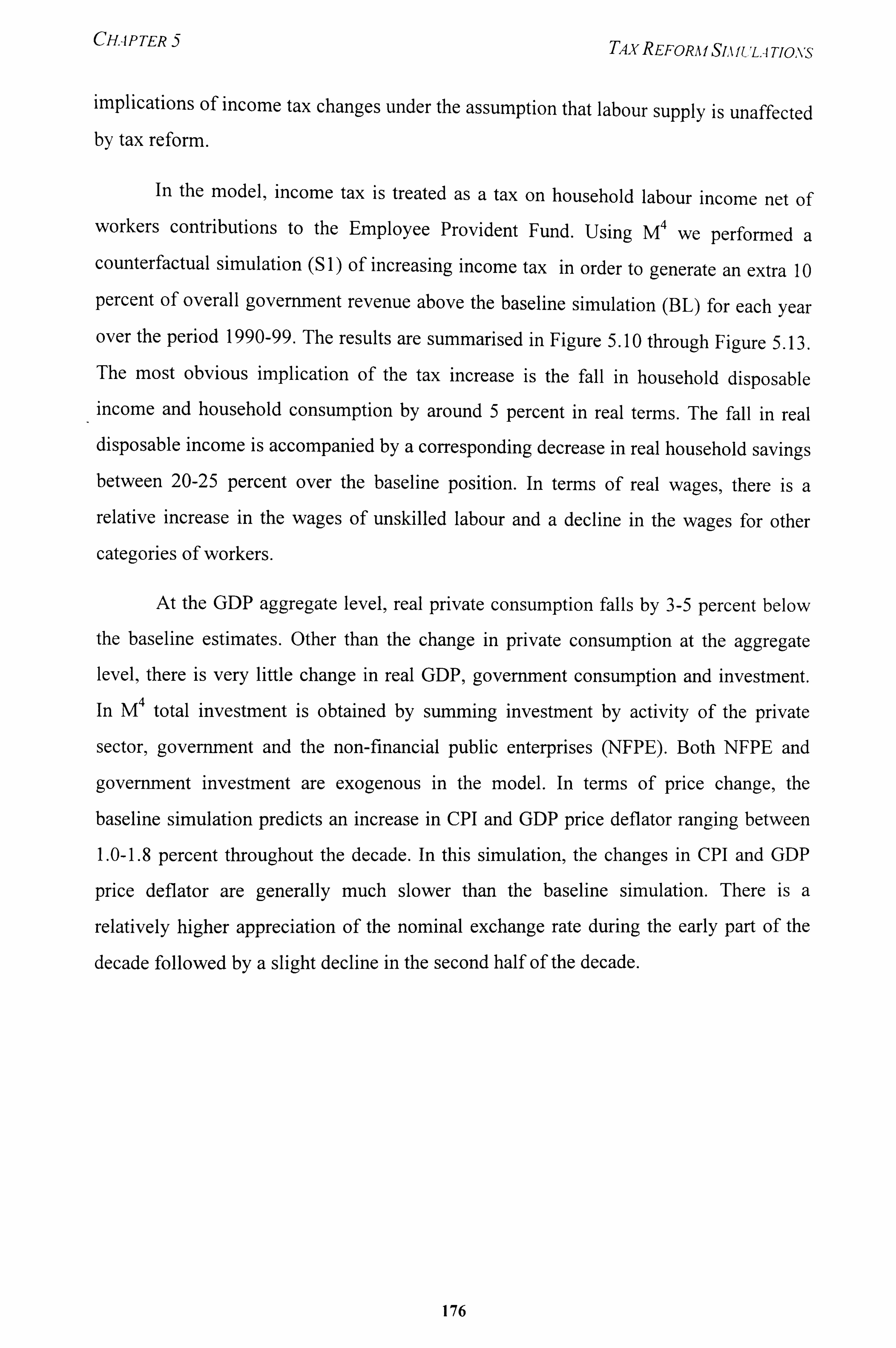
CHAPTER 5 TAx REFORA f SIA f UL4 TIOXS

implications of income tax changes under the assumption that labour supply is unaffected by tax reform.

In the model , income tax is treated as a tax on household labour income net of workers contributions to the Employee Provident Fund. Using M4 we performed a counterfactual simulation (S 1) of increasing income tax in order to generate an extra 10

percent of overall government revenue above the baseline simulation (BL) for each year over the period 1990-99. The results are summarised in Figure 5.10 through Figure 5.13. The most obvious implication of the tax increase is the fall in household disposable income and household consumption by around 5 percent in real terms. The fall in real disposable income is accompanied by a corresponding decrease in real household savings between 20-25 percent over the baseline position. In terms of real wages, there is a relative increase in the wages of unskilled labour and a decline in the wages for other

categories of workers.

At the GDP aggregate level, real private consumption falls by 3-5 percent below

the baseline estimates. Other than the change in private consumption at the aggregate level,, there is very little change in real GDP, government consumption and investment.

In M4 total investment is obtained by summing investment by activity of the private

sector, government and the non-financial public enterprises (NFPE). Both NFPE and

government investment are exogenous in the model. In terms of price change, the

baseline simulation predicts an increase in CPI and GDP price deflator ranging between

1.0-1.8 percent throughout the decade. In this simulation, the changes in CPI and GDP

price deflator are generally much slower than the baseline simulation. There is a

relatively higher appreciation of the nominal exchange rate during the early part of the

decade followed by a slight decline in the second half of the decade.

176

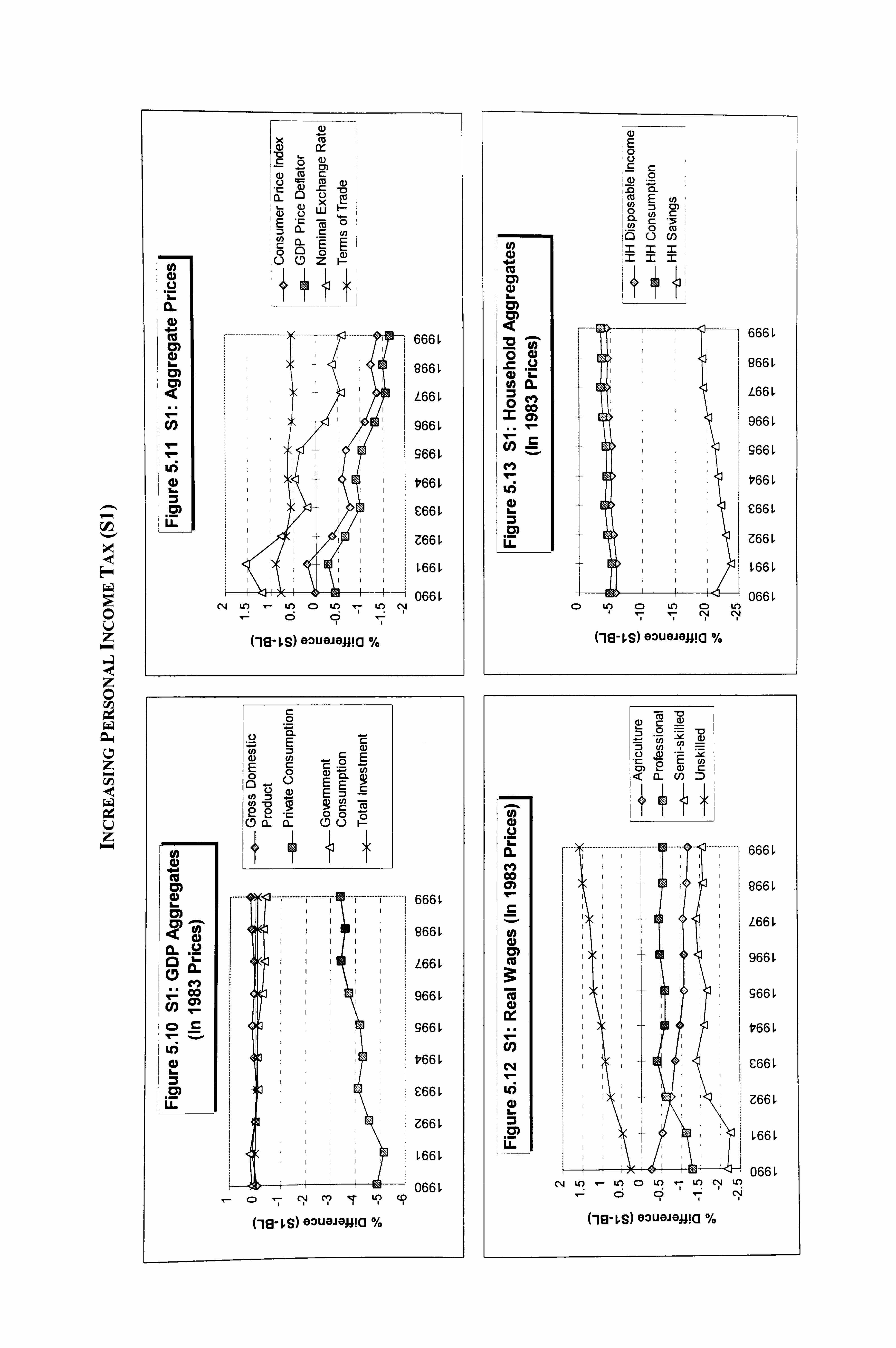
cl)

C

z -

z C (ID

z (ID

cu

.r cj -(D cm-- ,

c23) ý

X LLJ

cn 0 CL ýc F- Eý

666 L

966 L

L66 L

966 L

966 L

'066 L

C66 L

Z66 L

L66L

066 L 04 LO LO CD LO U') N

ci

(-le-W 03UGJG: U! a %

16. 0) r

c! )

ý ý: co

c 0 0

'ý - CL

Z 0 (1) Z 0 - r- 0 E

ý 0 o 92-

EE 9

en -0 9 EZ 9 U)

r -a

22 2 (D c)- -c CL

- 00 (D (-) -

---------- 666 ý

lR66 ý

L66 ý

9661

966 ý

V66 ý

C66

Z66 L

[66L

066 L Cý I? 'T 14?

cls-w eouojo: u! a %

1 (1) E 0

(D .2 70 lu CL E cn cn 0 :3 tm

c 1 "

o . cu U)

.1 1 666 ý 0

63 > ý0 CL -MI L66 L

0 co

I

966

Cl) 966 L

V66 L

C66 L

Z66 L

L66L

066 L 0 LO C) LO C) LO

(-le-m) eouejemia %

(1) 2

-ffi C -0 -

.2 (1) ýý A -D

75 L) . r-

U) 'R 2

T -ý -,. e cn

V) < 4) U) C: :D

........... ..... ........ ... . ....... ..... ...... 6661 CW) ýý ý I co I I 966

L66 ý

966

966

V66

ý 0) 111 1 1 i C66 L

L6 Z66 L

ý66L

066 L 04 LO LO C) U') Uý Cý U?

6 I 1

CN 1

(-113-W eouejema %

CHAP TER 5 TAx REFORA f SIA f ULA TIONS

6.1.2 Increasing corporate income tax (S2)

As discussed in Atkinson and Stiglitz (1980), the issues connected with the

effects of corporate income tax are more complex than is often assumed in econometric

studies. Corporation tax can take several forms and it depends on, among other things,

the tax deductibility of interest payments and the depreciation provisions. Tax policy

affects the capital structure of the firm and, accordingly, the marginal cost of capital. According to theory, as a result of corporate profits tax the cost of capital will rise and

cause the firm to adopt less capital -intensive technique at any level of output and to

switch from corporate to the non-corporate sector in their demand for factors. Hall and Jogenson (1967) undertook an investigation of taxation and investment. They showed

that the adoption of accelerated depreciation allowances in the United States following

the 1954 legislation reduced the cost of capital by 9 percent and accounted for a

substantial increase in investment. A cut in corporation tax from 52 to 48 percent in 1964

is estimated to have increased the cost of capital by I percent 21 and caused a small

reduction of investment. However, the results are still not firmly established because of

the considerable difficulties in making the transition from the theoretical model to the

empirical work. Corporate profits tax is also linked to the choice of factor intensity as

well as relative output demand in the corporate/non-corporate sectors. In addition, studies

have been conducted on the general equilibrium effects of investment tax credits against

corporate tax changes for promoting investments in developing countries. 22

17 Total government receipts are equal to the sum of its direct and indirect taxes, plus exogenous transfers from the

rest of the world plus the interest income that the government enjoys on claims it holds against financial

institutions. 18 There are two categories of government expenditure in Malaysia, namely, 'operating expenditure' and

'development expenditure'. Operating expenditure, which falls under the purview of Treasury, is allocated as part

of the annual budgetary exercise for the running of government, as well as other expenses borne by the government. In the model, government operating expenditure is defined as the sum of its current account expenditures on goo s

and services plus the sum of its transfers to other domestic institutions and to residents in the rest of the world. Transfers include service payments on government debt. Development expenditure is made for new government

investments and is allocated under the five-year Malaysia Plans, with provisions for a mid-term assessment. This

fund is controlled by the Economic Planning Unit.

19 In M4 the Government sector is narrower in scope than the 'Public Sector'. The Non-FInancial Public Enterprises

are separately identified in the model.

20 Government current surplus is defined as the difference between current account receipts and expenditures. Government financial surplus/deficit is obtained from subtracting the nominal value of government investment (or

'Development Expenditure') from government current surplus.

21 It is argued that this is the result of the depreciation provisions being in excess of true economic depreciation.

22 See Feltenstem and Shah (1993) for Pakistan and Feltenstein and Shah (1995) for Mexico.

178

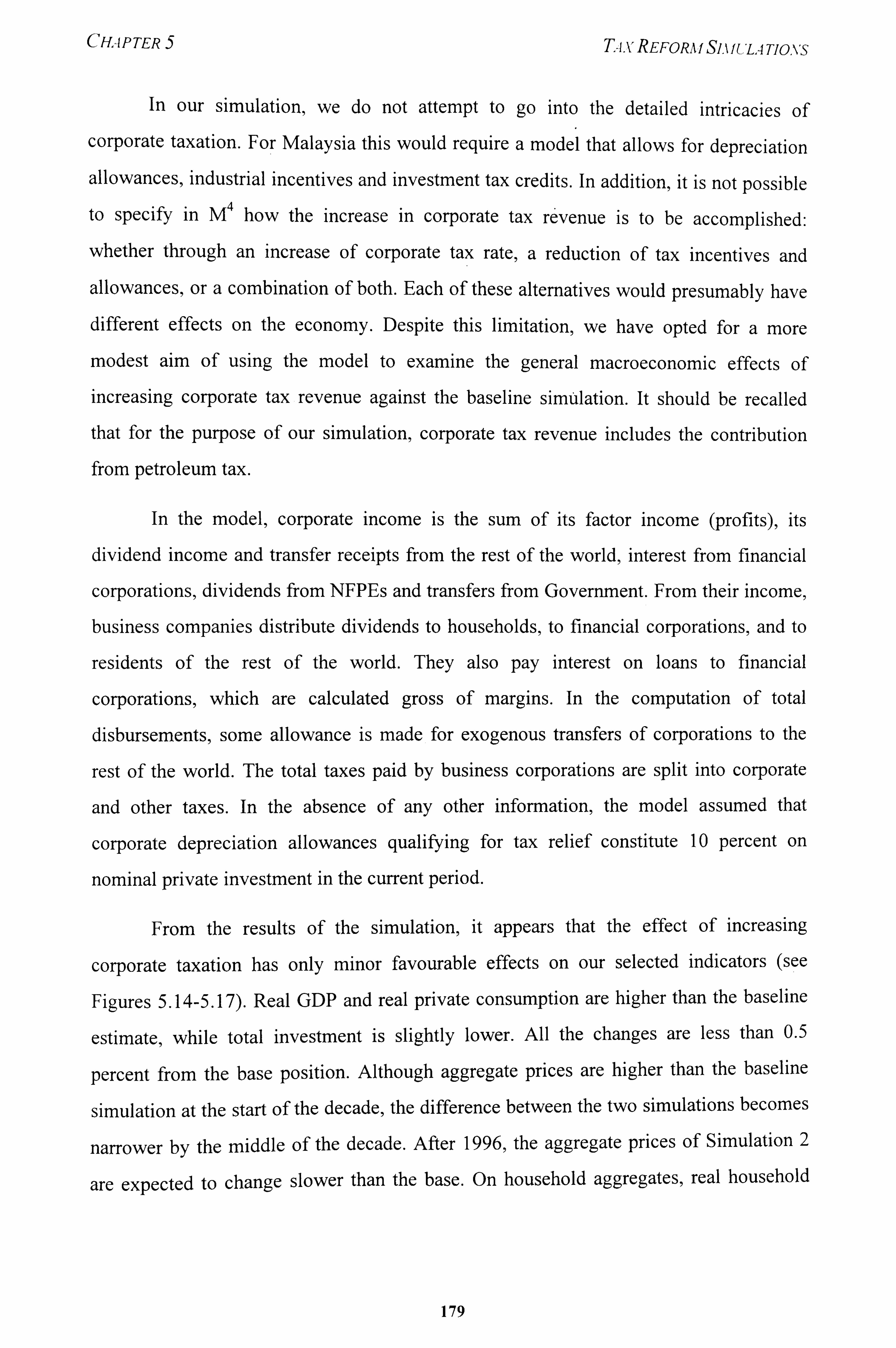
CHAPTER 5 T-i. VREFORAf SIAIULATIONS

In our simulation, we do not attempt to go into the detailed intricacies of corporate taxation. For Malaysia this would require a model that allows for depreciation

allowances, industrial incentives and investment tax credits. In addition, it is not possible to specify in M4 how the increase in corporate tax revenue is to be accomplished:

whether through an increase of corporate tax rate, a reduction of tax incentives and

allowances, or a combination of both. Each of these alternatives would presumably have

different effects on the economy. Despite this limitation, we have opted for a more

modest aim of using the model to examine the general macroeconomic effects of increasing corporate tax revenue against the baseline simulation. It should be recalled that for the purpose of our simulation, corporate tax revenue includes the contribution from petroleum tax.

In the model, corporate income is the sum of its factor income (profits), its

dividend income and transfer receipts from the rest of the world, interest from financial

corporations, dividends from NFPEs and transfers from Government. From their income,

business companies distribute dividends to households, to financial corporations, and to

residents of the rest of the world. They also pay interest on loans to financial

corporations, which are calculated gross of margins. In the computation of total

disbursements, some allowance is made for exogenous transfers of corporations to the

rest of the world. The total taxes paid by business corporations are split into corporate

and other taxes. In the absence of any other information, the model assumed that

corporate depreciation allowances qualifying for tax relief constitute 10 percent on

nominal private investment in the current period.

From the results of the simulation, it appears that the effect of increasing

corporate taxation has only minor favourable effects on our selected indicators (see

Figures 5.14-5.17). Real GDP and real private consumption are higher than the baseline

estimate, while total investment is slightly lower. All the changes are less than 0.5

percent from the base position. Although aggregate prices are higher than the baseline

simulation at the start of the decade, the difference between the two simulations becomes

narrower by the middle of the decade. After 1996, the aggregate prices of Simulation 2

are expected to change slower than the base. On household aggregates, real household

179

in.

FQ

ce u

z

0. -0

CL

cu ý IM

: CM

Lo

IM

cu

x ui

0 z

. .................... ..................... ............... - 666 ý

966 L

L66 L

966 L

966 L

V66 L

C66 ý

Z66 L

I L66L

066 L CR lp llý clý Cl CN It 0 CD 0 CD (; i c

(-113-ZS) 0: )UGJGJI! a %

I cc

16.

U)

a. A. ) a. ISO)

2M

LL

C:

.2 CL

E cn 0

=3 to 0 E

E 0

c 0 L) i; _- CL E

cn (D E

2 9 c cu 2 a- -r- CL 00

666 ý

966 ý

L66 ý

966 ý

966 ý

V66 ý

C66 L

Z66 L

L66L

066 (0 LC) . cr CY) C14 C) CN (Y) mt C: ) C) C: ) C: ) a c) C? 999

(-113-ES) GDUGJG-4! (3 %

1E 10

, -0 CL

E 0

c o c)

- 666 .2 oo . 0 966

CL m L66 L

0 co i

966

966

V66 L

C66 L

Z66 L

L66L

066 L 0) CO P- (D LO 10- M CN C)

(, 19-zs) eouejama %

(L) L C: - =3 .2

75 U .a S) - -ý -, ýe oI CD 2 a) lc < a_ U) Z)

CL 666

Co I I II

966

L66

1 966 L

966

V66

C66 L

Z66

ý66ý

066 vý clý C) C14 C") 'IT LO (-D

0 C) 0 Cý Cý Cý 9 Cý ý

99 Cý 9

(-113-ZS) GOUMMO %

CHAP TER T-ix REFORM SIMULA TIONS

disposable income and consumption are expected to rise to I percent of the baseline

estimates. Real household savings rise to around 9 percent above the base by the end of the decade. There is a slight improvement in real wages for agricultural workers and

unskilled workers and a worsening in the wages of professional workers and especially

semi-skilled workers.

6.1.3 Increasing export taxes (S3)

The contribution of export taxes to total tax revenue has been declining over the

years. The taxes are levied on primary commodities based on ad valorem rates and on the

excess of export prices over some notional cost of production. In the model, export taxes

are calculated by multiplying the ad valorem tax rates by the appropriate nominal flows

and then summing over all transactions on which export taxes are levied.

Simulation S3 is based on the assumption that the export tax rates are raised to

increase government revenue by 10 percent above the base simulation. The results of the

S3 compared with the baseline (BL) are shown in Figures 5.18-5.21. This simulation

results in a relative decline in real GDP of up to 0.5 percent of the base, and a sharper

decline in private consumption. The rise in export taxes leaves total investment

unchanged. In terms of the effect on aggregate prices, the GDP price deflator is higher

than the base by 2-3 percent, while the CPI remains unchanged during the initial years

but increasing up to 2 percent by the end of the decade. This is accompanied by an

appreciation in the nominal exchange rate and a worsening of the terms of trade.

Household disposable income and consumption are initially lower than the base

simulation by I percent and gradually falling to 4 percent by the end of the decade. Real

household savings are expected to record a steeper decline from 2 percent below the

baseline position in 1990 to around 13 percent in 1999. Increasing export taxes have a

negative effect on the real wages of professional, semi-skilled and unskilled workers.

Wages of agricultural workers seem to be least affected by the tax increase. This may

appear rather surprising since the traditional argument for lowering export taxes is to

reduce the regressive effects of the tax on the income of primary producers. However, it

is because of the regressive nature of the tax on poor households engaged in primary

commodities production that many of the export taxes have either been reduced or

removed during the late 1980s. By 1990 over 97 percent of export taxes collected were

181

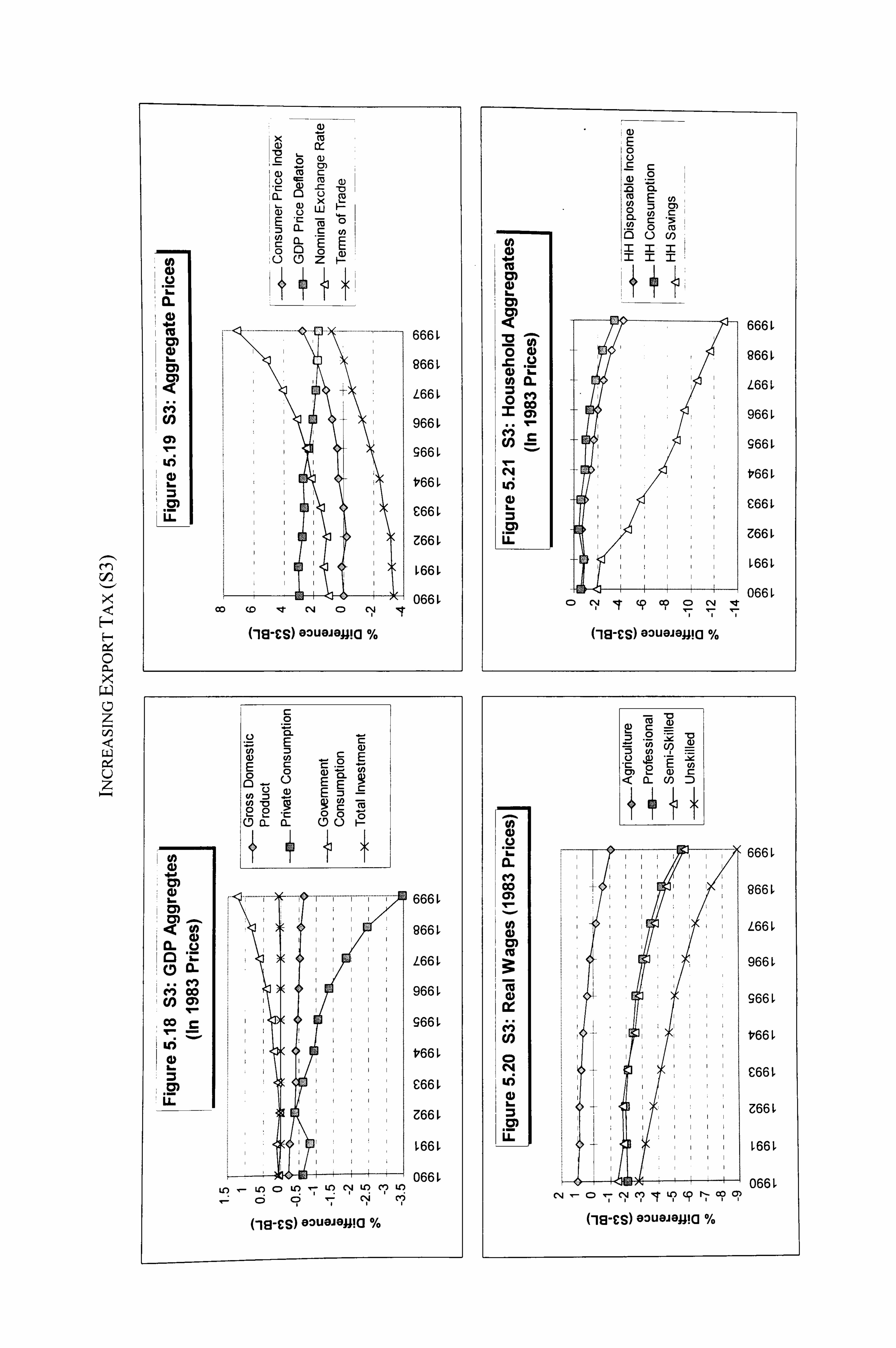
1--lý rn

CD

ý CM <

CY)

rn ý EL

x (U CY- ý -0

L- A0 Q)

M1 a) M r-

x 10

Lu

r CL

666 ý

966 L

L66

966 L

966

V66

C66

Z66 L

066 L co (D 1- 04 0 C\l

I

GDUGJG-4! (3 %

CL

ý C") co 00

LO

Co (L) Z (A - c:

0)

0 -ö

0 EE

cn m 9 22 0o (D u

0 co x C7) 4ýi TI, C cn

Tm N L6

E 1 0 0

.0 CL M 0 E 0 :3 CM :

0 (-) m

u)

666 L

966 ý

L66 L

966 L

966 L

1766 L

C66 L

Z661

L66L

066 L o c"q (9 c? c) C-4 'q-

- .01 2 -0 CO) (/) (U 75 W 4p

2 ( ,) (L) C Cl- co Z)

666

(Y) .III ý ýý co

0) .If ve iI

I 866

L66

966

(D 966

Cl) ;I V66 ý

C66

Z66

L66L

066 L CN Cl Cý 1? 4? 19 llý op 1ý

(-19-cs) eouejema %

CHAPTER 5 T4, v REFORA I SIA f ULA TIONS

derived from petroleum export, while the export taxes from rubber, tin and palm oil were

negligible.

6.1.4 Increasing import taxes (S4)

Import duties are levied on a wide range of imports. Most goods are charged rates between 10-35 percent. There is an additional surcharge of 2 percent for raw materials

and some machinery and 5 percent surcharge for other goods. The most important source

of import duty revenue comes from petroleum and fuel oil. Tax exemptions are given to

imports used by government and public enterprises as well as certain types of

investments. " Import taxes are calculated in the model by applying ad valorem tax rates

to the appropriate nominal flows and then summing over all transactions of imports for

intermediate, consumption and capital uses. Many CGE studies of the effects of trade

liberalisation use classical models in which all factors, including physical capital, are

freely mobile between sectors. In addition, commodity and factor markets are assumed to

be perfectly competitive. The results of these studies suggest that there are welfare gains,

though small , in liberalising trade.

Figures 5.22-5.25 show the results of the simulation for import taxes (S4)

compared with the baseline simulation. The model predicts that with an increase of

import taxes, there is relative decline in real GDP and real government consumption

between 0.5-1.0 percent. The decline in real private consumption is larger, between 3.0-

4.5 percent. There is also an increase in consumer prices and GDP price deflator up to

1997 and a depreciation in the nominal exchange rate of 1-2 percent. There is no change

for the terms of trade.

24 The MIER Tax Reform Group (1988) proposes that the current import system could be strengthened by abolishing

exemptions from import duties granted to government departments and public enterprises and introducing a near

uniform rate for most products.

183

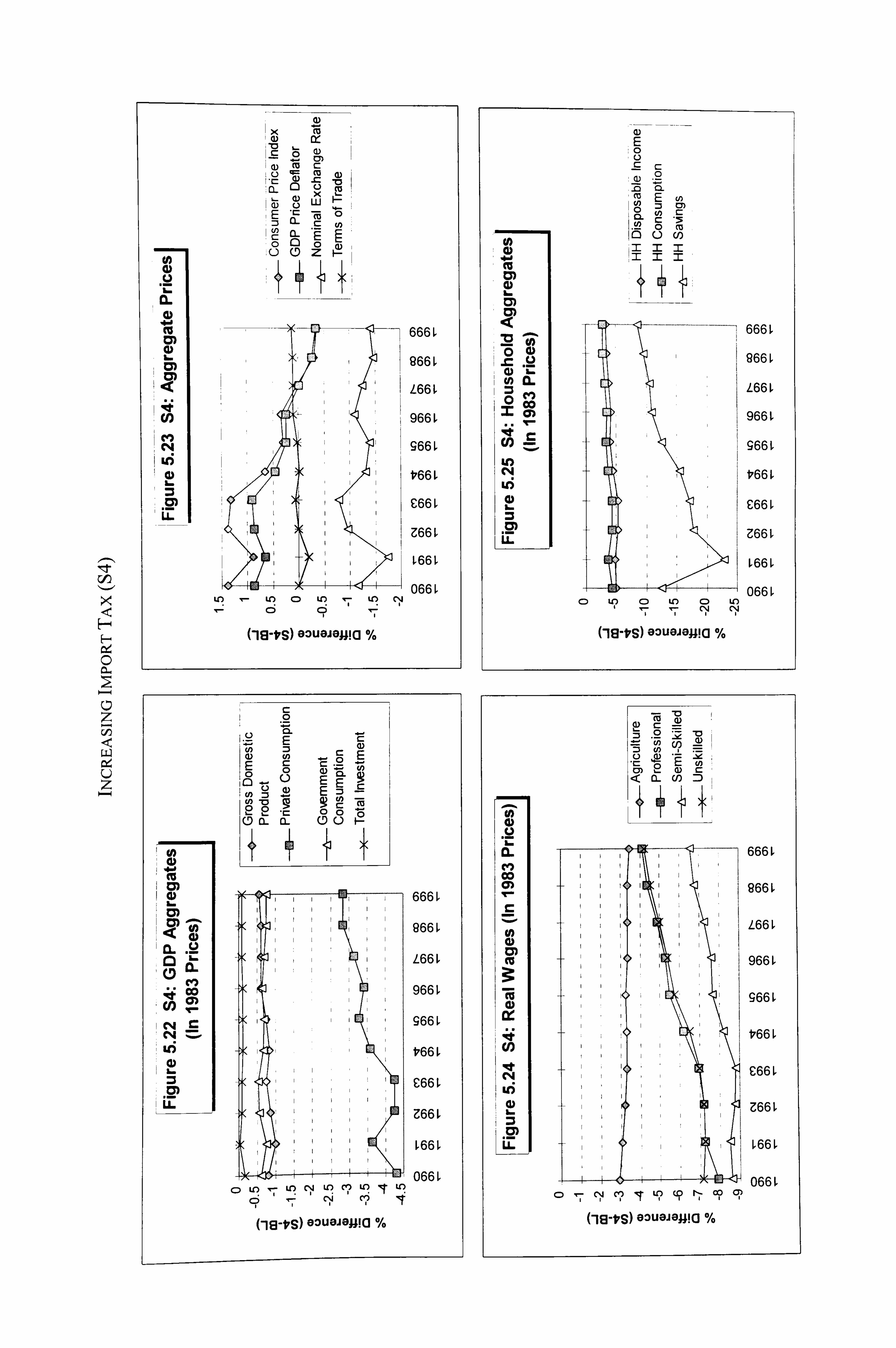
cl)

H

0

z cJ)

[. i

L) z

Lc;

M

xm cu

0 (1) MC

UJ D 0- C (n

ý (j) c Cl- Eý

10 (D z

666 ý

966 ý

L66 ý

966 ý

966 ý

V66 L

C66 L

Z66 L

ý66L

066 L Lq CD U) C4 C)

os-vs) e3uexama %

0

E

E 0 '= E

0 0 4) cl EE (n S?

C. ) = (L) - E

2 2 (D CL -r- IL

00 (D

666 ý

966 ý

L66 0-

4 co ý ý 966 L ;

C4 966 L N

V66 L

C66 L

Z66 L

L66L

066 L c) Lo u) Cý LO C? LO LC)

c; C14 C?

(D L.

U) 0

2 (D L. ch CL = Col 0 co

CM ui

CD

I 17L

Q)

CM 10 (A r-

666 ý

966 ý

L66

966 L

966 L

V66

C66 L

Z66 L

L66L

066 L LO C) LO C) LO Cý Cý

(113-VS) 03UGJG. 4! a %

:3 .0 in 1.1: -D

75 . 1-) U)

1-1) 2 *ý I < a- U) D1

U)

CL 666

co IIII I I I 966

L66 U)

966

cu 966 L 0)

-V66 L cn

C66 L

Z66 L

CL ML

066 L C) Cý C? L?

oe-vs) eouejema %

CHAP TER T-i. v REFORM SIA f ULA TIONS

Simulation 4 predicts that there will be a decline in real household disposable income and real household consumption of 3-5 percent compared with the baseline

position. The simulation output shows that both the import and export volumes are lower than the baseline simulation, which suggests a lesser degree of openness of the economy. The demand for imports falls as a result of lower disposable income among consumers. The model also predicts a slight decrease in exports that is stimulated by the appreciation

of the real effective exchange rate. GDP, government consumption and total investment

in real terms are all expected to show a slight decrease of less than 0.1 percent. In other

words, the change in the tariff regime is not expected to have any significant effect on aggregate output. Although a rise in the import tax rate should generate a negative effect

on the economy arising from more expensive products and intermediate goods, the effect is subdued because of the low substitution elasticities adopted in the model. Physical

capital is not freely mobile in M4 . The re-allocation of capital to its most productive uses

can only be brought about through new investment, thereby contributing to some degree

of inertia in the model.

6 1.5 Increasing domestic indirect taxes (S5)

This category of tax captures the other indirect taxes, such as excise duties, sales

tax, service tax, and the other indirect taxes. Excise duties are collected by the Customs

and Excise Department from licensed factories that produce excisable goods. The duties

are imposed when the product moves through the gate that is monitored by a customs

officer. Excise duties are levied on products for domestic consumption and not on

exports. Over 75 percent of the excise revenue are derived from fuel oils, petroleum

products and vehicles, and about 30 percent from alcoholic and soft drinks, and

cigarettes. Sales tax contributes a growing share to tax revenue in recent years. It is

levied on manufacturing activity and excludes retail trade. Only the larger manufacturers

are subject to sales tax. Licensed manufacturers are entitled to claim tax credit on sale of

products to other manufacturers in the 'ring system'. Service tax is imposed on certain

services, such as lodging, entertainment, body services and other services. Other indirect

taxes are road tax and stamp duties. As with the case of export and import taxes, the

model calculates domestic indirect taxes by applying ad valorem tax rates on the

ap ropriate nominal flows. . rp I

185

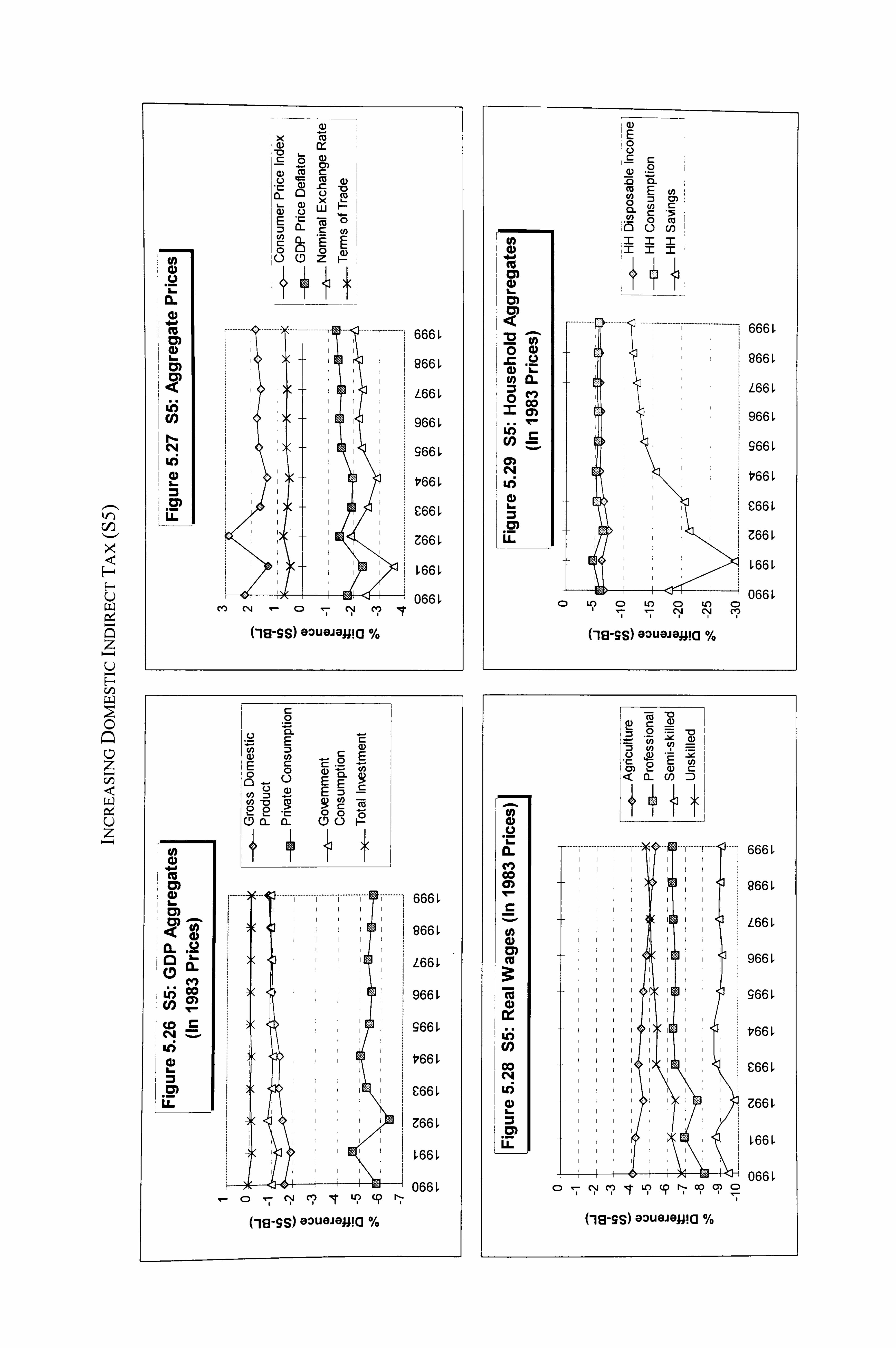
tI

F-

LL

z F- C/D

0

[L

C-)

z

IL

1 C4

&Z

mm LL

-0 j- .2

0- 0 c) M, x

LU

Z 0- r- w (n c a- ý9

Z

-- - ----- - -- --- ------ 666

966

I L66

i 966

966

'066

C66

Z66 L

L66L

c') CN C, Cý C7 I-

(-le-gs) eouejema %

U) 4)

rin '0-ý

a. C) 16.

0 CL

0) U) T"

to a cl Z1-

Lo

LL

0- 0 Co :3 0 (V

- cn m 9 9 Co r -ffi 22 CL -r- CL

- 0

........... ............ ............. 666

8661

1 L66 L

966

966 L

V661

C66

Z66

'IT 19 19

ODUGJGH! O %

ý cn

ý Z:

16.

-0 c2-

lu In Z cm

..... ....... 6661

966 L

L66

966

966

V661

C661

Z66

ý66ý

1 -4- 0661 LO C) LO C) LO a

(-le-gs) eouejema %

-ffi -0

cn . c. ) ( L) -E

--N: 2

U) %

CL .......... .......... .......... 666

co (7) 8661

C Z-ý -- II L66 L U)

cu ýIIIIII1 966 ý

966 L

V66 L

co C66 L N

Z66 L

L66L JLJ

066 L 0.1 cn 'T L9 1.9 C9 1ý C,

(-le-gs) eouejo: u! a %

CHAPTER 5 TIxREFoRvi Si. ý f uL, _1 Tjo. vs

The increase of domestic indirect taxes has a negative effect at the aggregate GDP

as well as household level. Real GDP and real government consumption decline by

around 1-2 percent of the baseline position, while real private consumption falls by 5-6

percent. Higher excise duties on fuel oils, petroleum products and vehicles as well as higher sales tax contribute to higher prices which are passed on to consumers. The CPI

rises by about 2 percent above the baseline simulation. There is a slight depreciation of The nominal exchange rate depreciates slightly and increases the competitiveness of

exports, contributing to an increase in net exports. At the household level, real household

disposable income and consumption declines by about 5 percent (see Figure 5.29).

6.1.6 Increasing non-commodity taxes (S6)

In Simulation 6, non-commodity taxes are raised to generate additional 10

percent revenue for the government. Non-commodity taxes on production are calculated

as an ad valorem mark-up on the (net factor cost) price of value-added. This tax rise

leaves real GDP, government consumption, and total investment practically unchanged

over the base position. Real private consumption, however, declines between 2.5-4.0

percent. The nominal exchange rate and CPI are expected to decline within one percent

from the base. The GDP price deflator initially rises to around 4.5 percent above the base

at the start of the decade, but later falling to around 2 percent. The negative effects of

increasing non-commodity taxes are felt more strongly at the household level. Real

household disposable income and real household consumption decline by 2-4 percent,

while real household savings fall between 10-14 percent over the base position. This

decline has partly been caused by the real wages for four categories of workers falling by

4-7 percent during the decade.

6.2 Revenue-Neutral Tax Simulations

In this section, we perform the second group of counter-factual simulations by

varying two groups of taxes simultaneously so that the tax reform is revenue neutral.

This set of simulations will answer the question whether there could be some economic

and welfare gains from changing the existing tax structure without fundamentally

affecting the revenue position of the Federal Government projected under the baseline

187

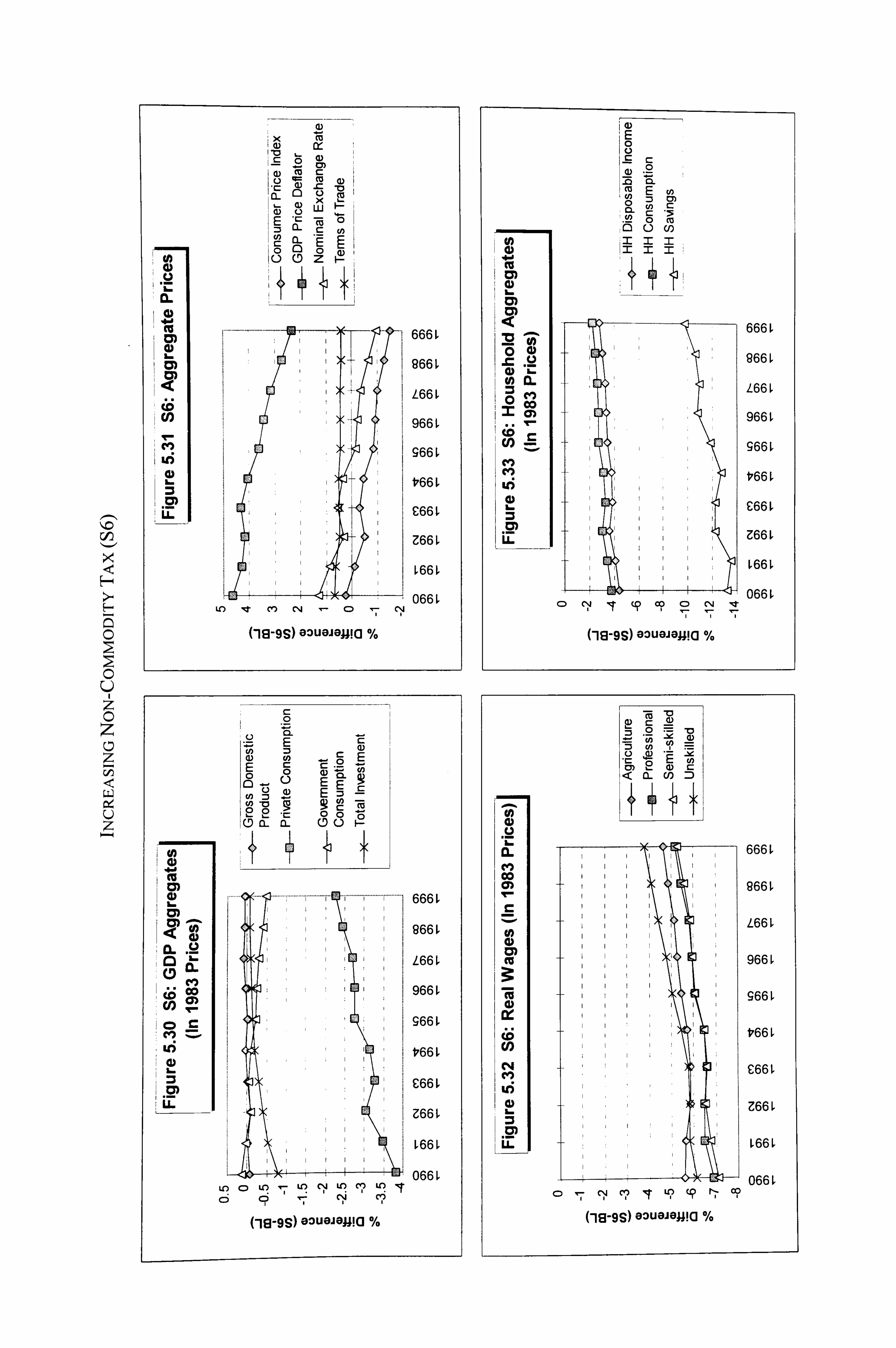
C

0 L 7 0

z

Li.

U z

IL

1 CF)

1 0)

LL

X

CL) C. )

W Cl- 00

(D

E = a- c ch I CL

0

i .1 11

6661

966 L

L66

966 L

966

V66 ý

C66 ý

Z66 L

L66ý

066 U') cT CO C%4 C=) 04

(-18-9S) 0: )UGJGII! (3 %

ý Im oýft

can 2

ý J: k; Go

!0C

Lc;

c .2 CL E

CD E

=3

'ZZ 0 0 0 C) (a. EE 9

(n (n -0 CD

5 E S? (n

c -ffi 2 CL CL 00 -

............ .......... ... ........ 666

966

L66

9661

966

V66 L

C66

Z66

066 U-) a Lo U") Cý "I C? "I C) C? -1 Cý C?

(-113-9S) 0: )UGJG: U! (3 %

m .0

a. CW) co

1-7- (D

E 0

.0 CL

(13 E 0 cn CL c To cl C)

6661

966

1-66

966 L

9661

V661

C66

Z661

L66L

066 c) C'i 'T (9 0? c) C'4 "*-

(-113-9S) GOUGJG-4! (3 %

.2 U) -5 U) L)

< a- U) Z)

CL 666

co IIIII 0) 966

L66 L

966 L

966 L

V66 L

C66 L

Z66 L

L66L

066 L Cý C? C9

(-18-gs) eouejema %

CHAPTER. 5 T4-vREFORA f SIA f ULA TIONS

simulation. Two simulations are performed here. The first considers the effect of reforming direct taxes, while the second examines the implications of reforming indirect taxes through the introduction of value added tax.

6.2.1 Reducing personal income tax and increasing corporate tax (S7)

In this simulation, personal income tax revenue is reduced by 10 percent throughout the decade. This reduction is balanced by increasing corporate tax such that

the net effect of this tax reform leaves the yearly government revenue unchanged from

the baseline position. As shown in Simulation 1, a rise in personal income tax has a

negative effect on household income and real wages. This is not the case with raising

corporate tax. It is useful to bear in mind that although corporate tax revenue can raised by increasing the corporate tax rate, it is by no means the only way of raising revenue from this source. Changes in depreciation allowances, investment subsidies, tax holidays

and other breaks will affect the amount of revenue collected from this source.

One way of raising corporate tax revenue in Malaysia is trimming the industrial

tax incentives. According to the Financial Survey of Limited Companies (Department of

Statistics, 1988), foreign non-manufacturing firms paid 40 percent of their profits in

taxes against 44 percent for domestic non-manufacturing firms. Generally, manufacturers

pay lower taxes as the result of business tax incentives, which amounts to providing tax

subsidy to industry. In fact, some businesses benefit more from these incentives than

others. Foreign manufacturers pay 15 percent of their profits in taxes compared to 29

percent for domestic manufacturers. At Malaysia's current state of economic

development, it has still not been ascertained whether business tax incentives help to

increase inward foreign direct investment (FDI) or to give domestic firms an edge in

world trade competition. There was a proliferation of 'pioneer status' firms with the

introduction of the Promotion of Investment Act 1986. In addition, there are other

incentives, such as the Investment Tax Allowances (ITA), Industrial Adjustment

Allowances, abatements, and specific export incentives, which reduce the corporate tax

paid by companies. The direct costs of these incentives to the government are the

revenue foregone and a reduced tax base. Society loses as a result of the lower pre-tax

profits of firms that take full advantage of the incentives available. Notwithstanding the

inherent difficulty of attributing and quantifying the effects of specific incentives with

189

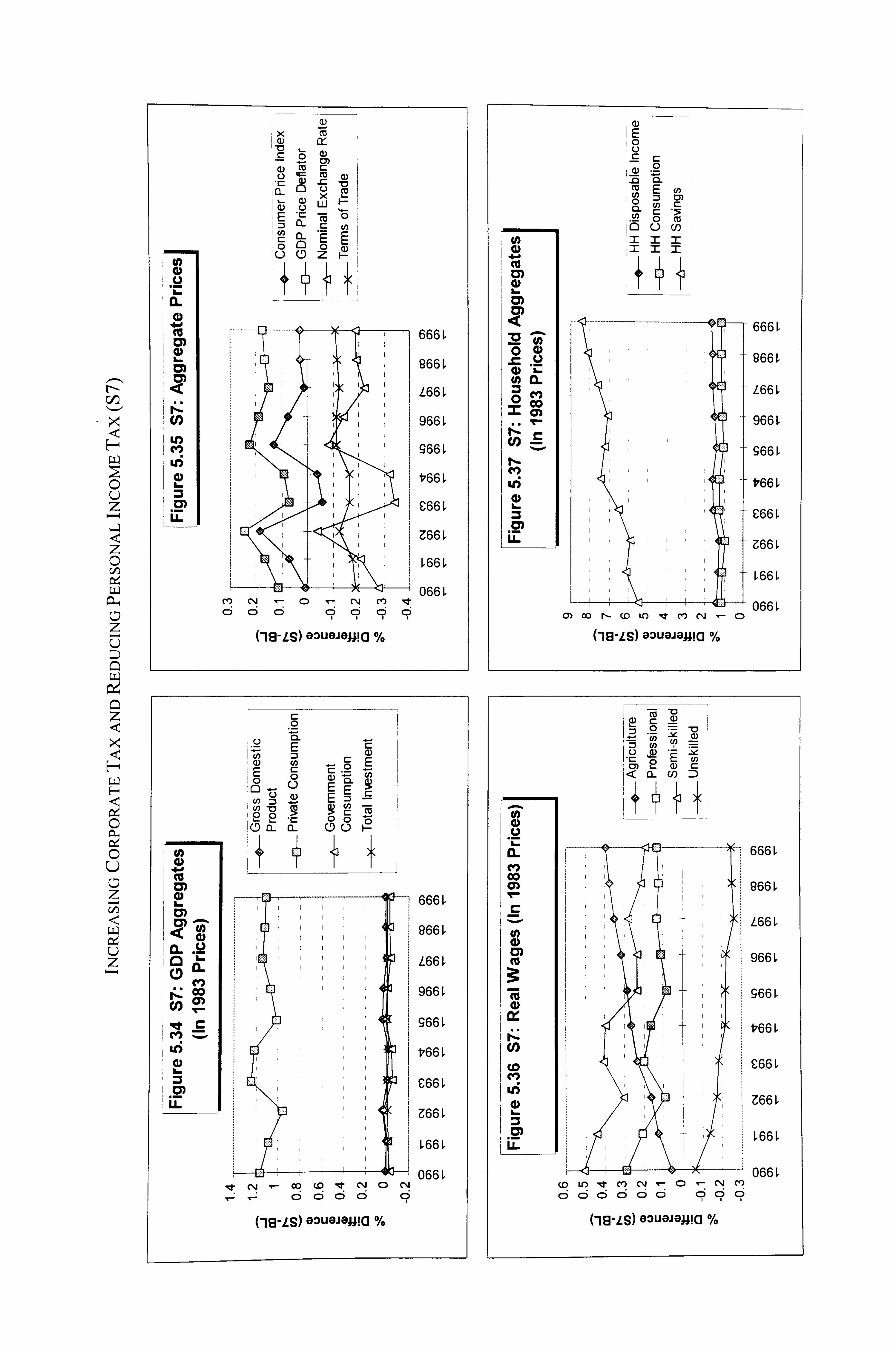
N rID

H

0 L) z -

z 0 1-J

z U

z

H Li.

H

0

0 C-)

tdD

Li- U z

CL

ý 0)

Lo m LO

LL

m 1-. (U A .2 cm

, Q) MC 1M ý. r M

x LU

i :3 0- a :r 92- EFý ý (-) (D Z F2 ý

666

966

L66

966

966

V66 L

C66 L

Z66 L

L66L

066 L M clý M C: ) ci c:, qqq

(-113-Ls) Gouejema %

4) I-

IL Ad C) CL

co

L6

ý 0) ýT

.2 0. E i

c C 2 E

10 0 c. E

L) =3 E E

U) -0 5 9 c: -ffi 2 a- - E- CL 00

W E

1 C)

i

m m t 2- E oý U) 0 cm ! r 0 m 0 co

M Z: 1: M Z: :C

666

0 Pffl

L66ý

966ý (0 Z ,1 : -- 966k

t, 66ý

£66ý

Z66ý

066ý C» 00 r- (D U«) le CY) CIJ CD

(-ii3-1s) a zuajawa %

-a -D 'a) c :3 .2= -0 ý -0 -X CD 75

W- * r_ CD cy) 2 a) r- IL U) Z)

0. i I 6661

co i

IIIIII

966

L66

966 L

966 L

V66 P-

C66 L

Z66 L

ý66L

... 066 L Ic! U? llý CY) cv -0- Cý clý

C) oo ci ci C5 6 C: ) II c) I (-18-LS) GOUBJGJI! O %

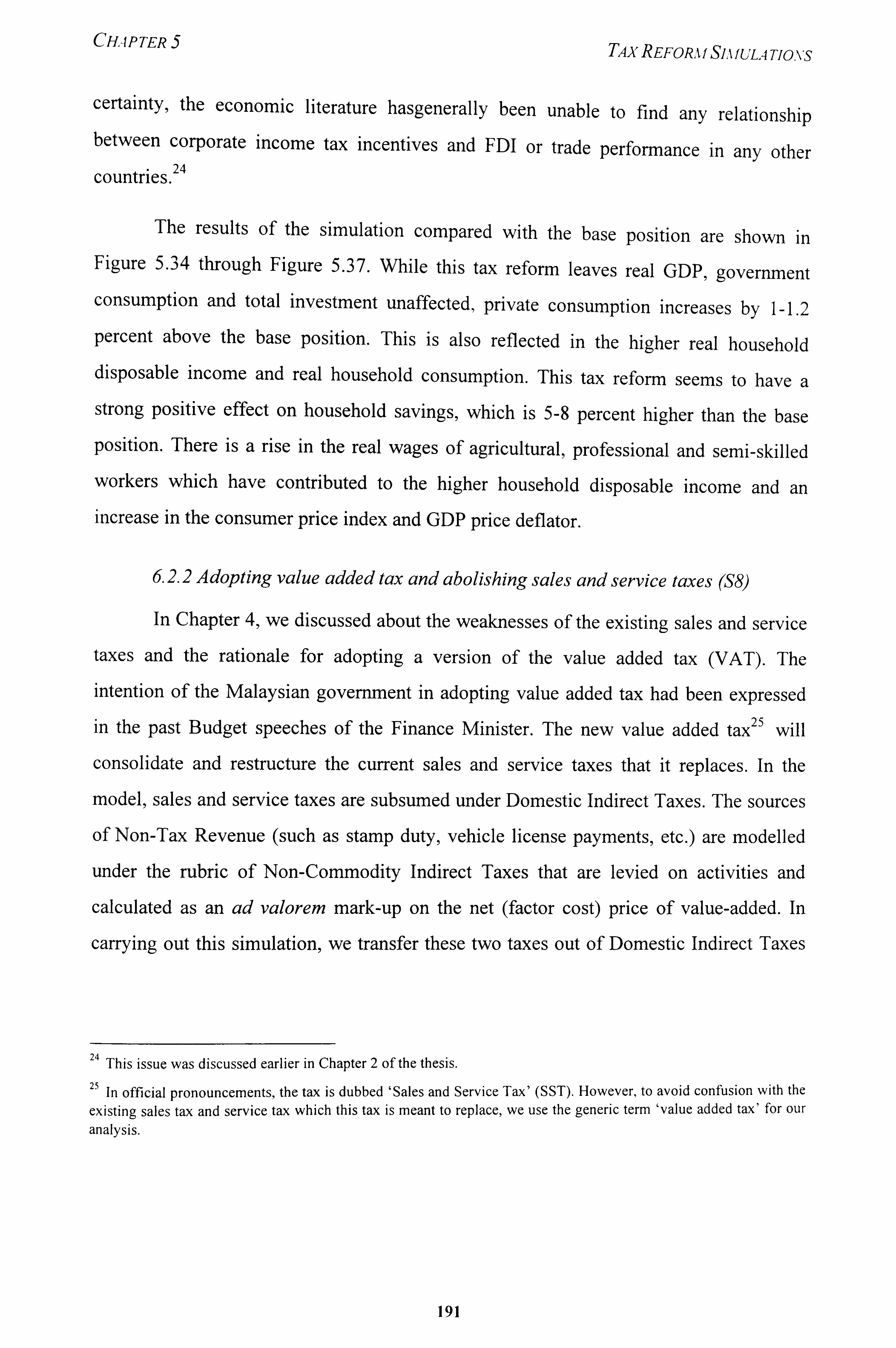
CHAPTER 5 TAX REFORA f SIA fULA TIONS

certainty, the economic literature hasgenerally been unable to find any relationship between corporate income tax incentives and FDI or trade performance in any other countries. 24

The results of the simulation compared with the base position are shown in Figure 5.334 through Figure 5.37. While this tax reform leaves real GDP, government consumption and total investment unaffected, private consumption increases by 1-1.2

percent above the base position. This is also reflected in the higher real household disposable income and real household consumption. This tax reform seems to have a strong positive effect on household savings, which is 5-8 percent higher than the base

position. There is a rise in the real wages of agricultural, professional and semi-skilled workers which have contributed to the higher household disposable income and an increase in the consumer price index and GDP price deflator.

6 2.2 Adopting value added tax and abolishing sales and service taxes (S8)

In Chapter 4, we discussed about the weaknesses of the existing sales and service taxes and the rationale for adopting a version of the value added tax (VAT). The

intention of the Malaysian government in adopting value added tax had been expressed

in the past Budget speeches of the Finance Minister. The new value added tax 25 will

consolidate and restructure the current sales and service taxes that it replaces. In the

model, sales and service taxes are subsumed under Domestic Indirect Taxes. The sources

of Non-Tax Revenue (such as stamp duty, vehicle license payments, etc. ) are modelled

under the rubric of Non-Commodity Indirect Taxes that are levied on activities and

calculated as an ad valorem mark-up on the net (factor cost) price of value-added. In

carrying out this simulation, we transfer these two taxes out of Domestic Indirect Taxes

24 This issue was discussed earlier in Chapter 2 of the thesis. 25 In official pronouncements, the tax is dubbed 'Sales and Service Tax' (SST). However, to avoid confusion with the

existing sales tax and service tax which this tax is meant to replace, we use the generic term 'value added tax' for our analysis.

191

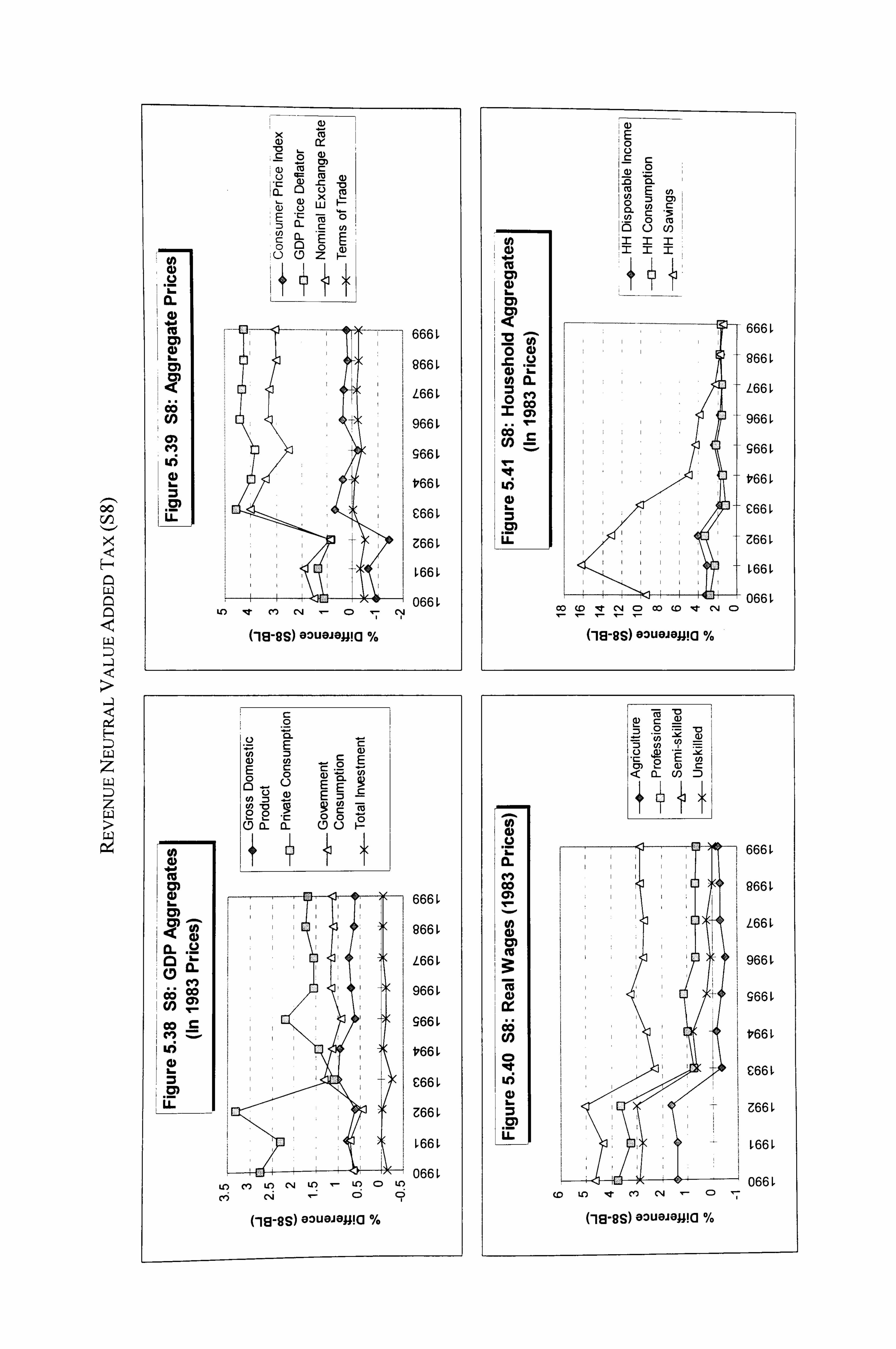
00

Lu) a, 0

i.

a) a, I..

I

x CD -0 L-

igo 4) 0)

Lu C5 :3 cl- c (n ý

0 z

16.

, 0- IZ(D'

16-

ý i6 Co Co r-

EL

EE 0 0= 0 -0

(1) - 9 90 ýa

ci- (DO

666

9661

L66

966

1 9661

V661

C66

Z66

066 U) cv) U-) 04 Lo C) to

cli C-ý ci

Cie-ss) eouoje;; ia %

E 0 1 L) cl) 10 E 0 ý cn =3 0 cn

. ý (m

C1

- . c 0 ! .I m

(a 11: 1: m (D : Z: M: a: i

666

0 966ý

/-66L 0 co i I 966 L

co 966L

V66L

C66L

Z66 L

L66L

066 L co (D C4 C) 00 (0 C%4 C)

(-le-os) eouejema %

75 0 ju - . r cm 2 < 0-

666

i CW) 1 Co

111 266 ý

Z66

966

966

U) t66 k

CD lqt £66

366 L2

02 7 L66ý

066 (0 LO mt CO (14 C: )

azueiawa 0/.

CHAPTER 5 T-i. v REFORA I SLI IULA TIONS

TABLE 5.4 CONTROL TOTALS FOR SIMULATION ON VALUE ADDED TAX

Domestic Non-Commodity Sales Tax & DIT-STST NC T+ VA T Indirect Taxes Tax (NCT) Service Tax Control Control

(D I T) (S TS T)

1990 5,452 6,776 2,563 2,889 9,339

1991 6,444 69387 2,897 3,547 9,284

1992 7,297 8ý075 3,404 3,893 11,479

1993 8,800 7,439 4,081 41719 11,520

1994 9,654 79958 4ý419 5,235 12,377

1995 10,691 51680 4,871 55820 10ý551

Source: Calculated from Economic Report (Ministry of Finance, 1995). Assumption: The introduction of VAT is intended to replace the revenue lost from repealing sales and service taxes.

to the Non- Commodity Indirect Tax. The control totals for Domestic Indirect Taxes and

Non-Commodity Tax are shown in Table 5.4. The rates for the two taxes are scaled

accordingly such that government revenue remains unchanged. In lieu of better data on

the anticipated revenue from sales tax and service tax for 1996-99, we assume that the

two tax indices for 1995 apply throughout the remaining years of the decade. Compared

to the base position, the shift to value added tax is accompanied by an improvement in

real household disposable income and real consumption. Consumer prices fluctuate

within one percent of the base position. Gross domestic product and government

recurrent expenditure register are higher by 0.5 - 1.0 percent than the base. There is also an

improvement in real private consumption throughout the decade. The adoption of value

added tax would have a slight effect in stimulating exports and imports, with a slight gain

in net exports.

There has always been a worry on the part of policy makers and members of the

public that the adoption of VAT would contribute to increases in retail prices. The

simulation shows that the consumer price index is expected rise by no more than I

percent following the shift from sales and service taxes to VAT. It will be maintained at

that level from 1993 onwards. As discussed in Chapter 3, VAT would address the

problem of tax cascading encountered in the sales and service taxes that contribute to

193

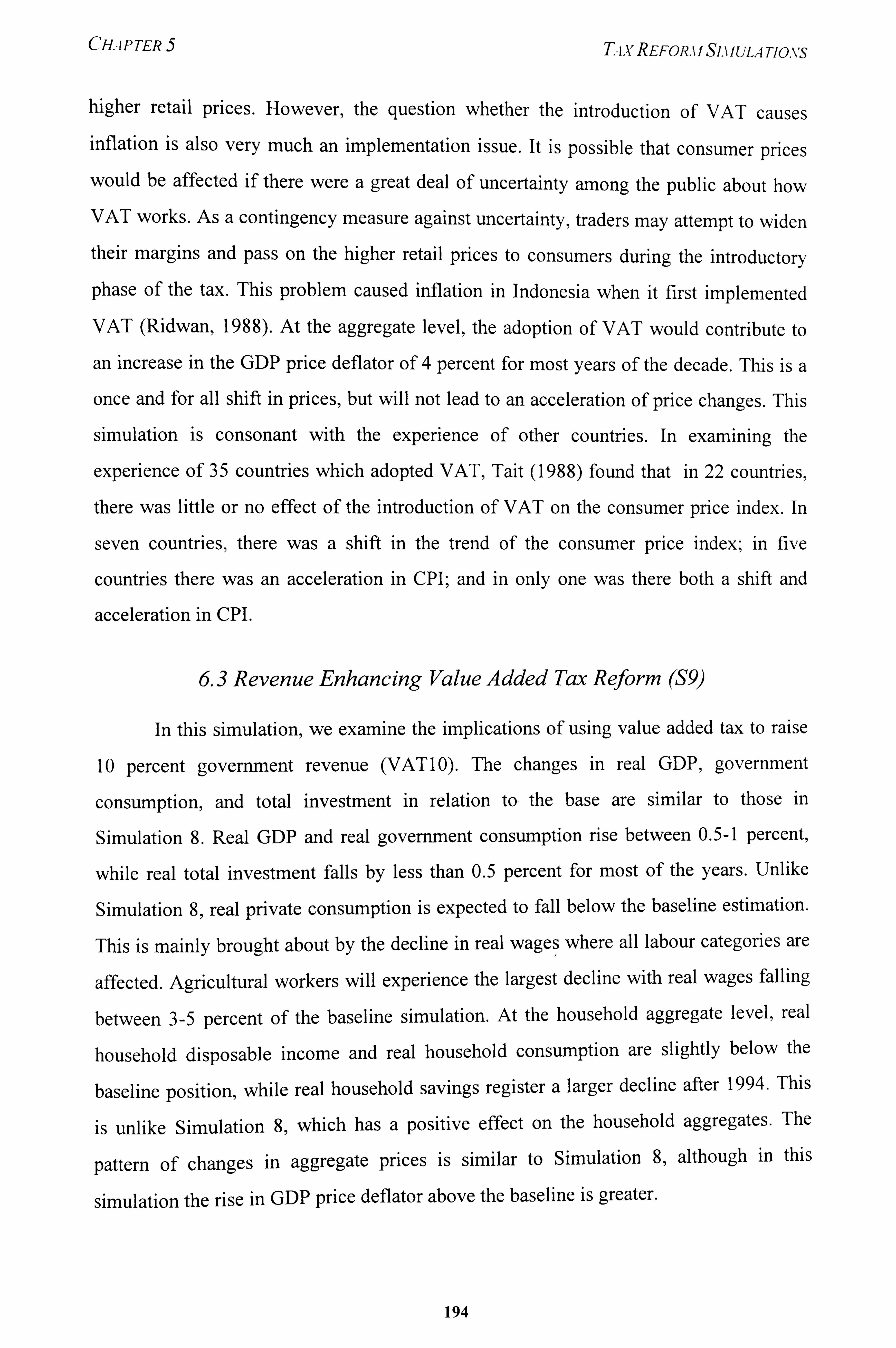
CHAPTER 5 T-i, vREFORA f SI. k IULA TIONS

higher retail prices. However, the question whether the introduction of VAT causes inflation is also very much an implementation issue. It is possible that consumer prices would be affected if there were a great deal of uncertainty among the public about how VAT works. As a contingency measure against uncertainty, traders may attempt to widen their margins and pass on the higher retail prices to consumers during the introductory

phase of the tax. This problem caused inflation in Indonesia when it first implemented

VAT (Ridwan, 1988). At the aggregate level, the adoption of VAT would contribute to

an increase in the GDP price deflator of 4 percent for most years of the decade. This is a

once and for all shift in prices, but will not lead to an acceleration of price changes. This

simulation is consonant with the experience of other countries. In examining the

experience of 35 countries which adopted VAT, Tait (1988) found that in 22 countries,

there was little or no effect of the introduction of VAT on the consumer price index. In

seven countries, there was a shift in the trend of the consumer price index; in five

countries there was an acceleration in CPI; and in only one was there both a shift and

acceleration in CPI.

6.3 Revenue Enhancing Value Added Tax Reform (S9)

In this simulation, we examine the implications of using value added tax to raise

10 percent government revenue (VAT10). The changes in real GDP, government

consumption, and total investment in relation to- the base are similar to those in

Simulation 8. Real GDP and real government consumption rise between 0.5-1 percent,

while real total investment falls by less than 0.5 percent for most of the years. Unlike

Simulation 8, real private consumption is expected to fall below the baseline estimation.

This is mainly brought about by the decline in real wages where all labour categories are

affected. Agricultural workers will experience the largest decline with real wages falling

between 3-5 percent of the baseline simulation. At the household aggregate level, real

household disposable income and real household consumption are slightly below the

baseline position, while real household savings register a larger decline after 1994. This

is unlike Simulation 8, which has a positive effect on the household aggregates. The

pattern of changes in aggregate prices is similar to Simulation 8, although in this

simulation the rise in GDP price deflator above the baseline is greater.

194

riD

L) z z Li.

z >

U)

Im

cam

L6

x

0 MC

Ci u (2 ý x LU

E :3 0- r- cn in c 0- EP 0 C) 0 (D Z

E .2 0 C= E

0- a E a) 0ý EE

0 9

C. ) (A =

2 2

:3

C E :3

0

c

- ý(D CL CO) 0 L)

666

966 L

L66 L

CL ! (D 966

CW) 1

6; CO 1 i

(j fj (j I CN s Iýý i V66 LO

C66

LL Z66

ý66ý

066 Uý 0 Uý Cý C)

('18-6S) %

ý 0)

cn

00 M0 CL) r-

=O: ce30 Zm ý da; ý CO r-

ý C. )

ý In Z ch ý

666 L

966 L

L66 L

1 966 L

966 L

V66 L

C66 L

Z66 L

L66L

066 L C. 0 "t C'4 0 C14 IT (9 Cq

I

(18-6S) GOUMMO %

.2 cn cp M U)

.0 -lu 2 *ý ý:

-1 a CD

Aj

666 L

co i I

866

L661

966

966

-066 Cl)

C66 ui

Z66 L

ý66L

066L Cý I? (-113-6S) OOUGJG: U! Cl %

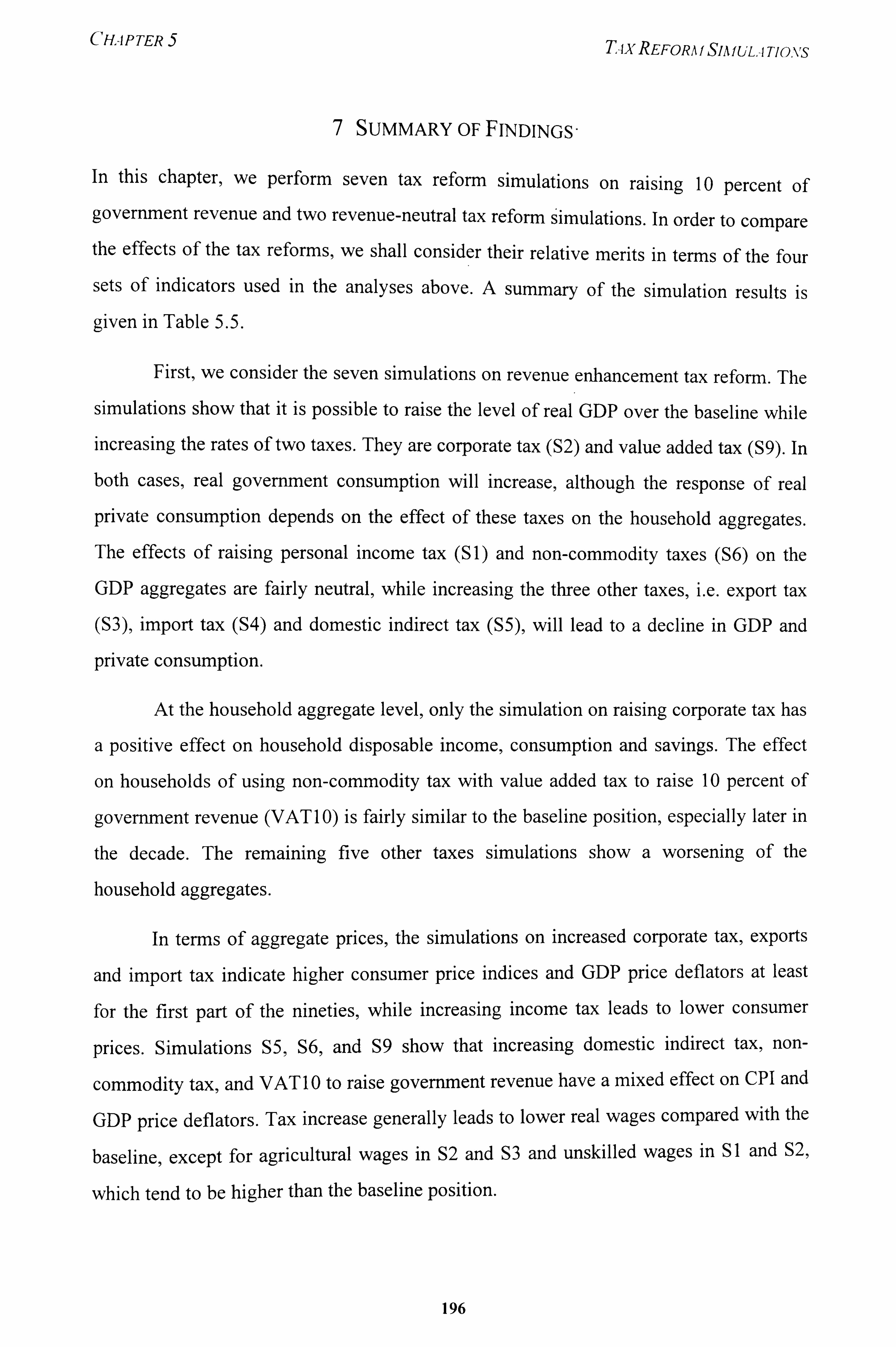
CHAP TER 5

7 SUMMARY OF FINDINGS,

T-ix REFORA f SIA f ULA TIONS

In this chapter, we perform seven tax reform simulations on raising 10 percent of government revenue and two revenue-neutral tax reform simulations. In order to compare the effects of the tax reforms, we shall consider their relative merits in terms of the four

sets of indicators used in the analyses above. A summary of the simulation results is given in Table 5.5.

First,, we consider the seven simulations on revenue enhancement tax reform. The

simulations show that it is possible to raise the level of real GDP over the baseline while

increasing the rates of two taxes. They are corporate tax (S2) and value added tax (S9). In

both cases, real government consumption will increase, although the response of real

private consumption depends on the effect of these taxes on the household aggregates. The effects of raising personal income tax (Sl) and non-commodity taxes (S6) on the

GDP aggregates are fairly neutral, while increasing the three other taxes, i. e. export tax

(S3), import tax (S4) and domestic indirect tax (S5), will lead to a decline in GDP and

private consumption.

At the household aggregate level, only the simulation on raising corporate tax has

a positive effect on household disposable income, consumption and savings. The effect

on households of using non-commodity tax with value added tax to raise 10 percent of

government revenue (VAT 10) is fairly similar to the baseline position, especially later in

the decade. The remaining five other taxes simulations show a worsening of the

household aggregates.

In terms of aggregate prices, the simulations on increased corporate tax, exports

and import tax indicate higher consumer price indices and GDP price deflators at least

for the first part of the nineties, while increasing income tax leads to lower consumer

prices. Simulations S5, S6, and S9 show that increasing domestic indirect tax, non-

commodity tax, and VAT 10 to raise government revenue have a mixed effect on CPI and

GDP price deflators. Tax increase generally leads to lower real wages compared with the

baseline, except for agricultural wages in S2 and S3 and unskilled wages in Sl and S2,

which tend to be higher than the baseline position.

196

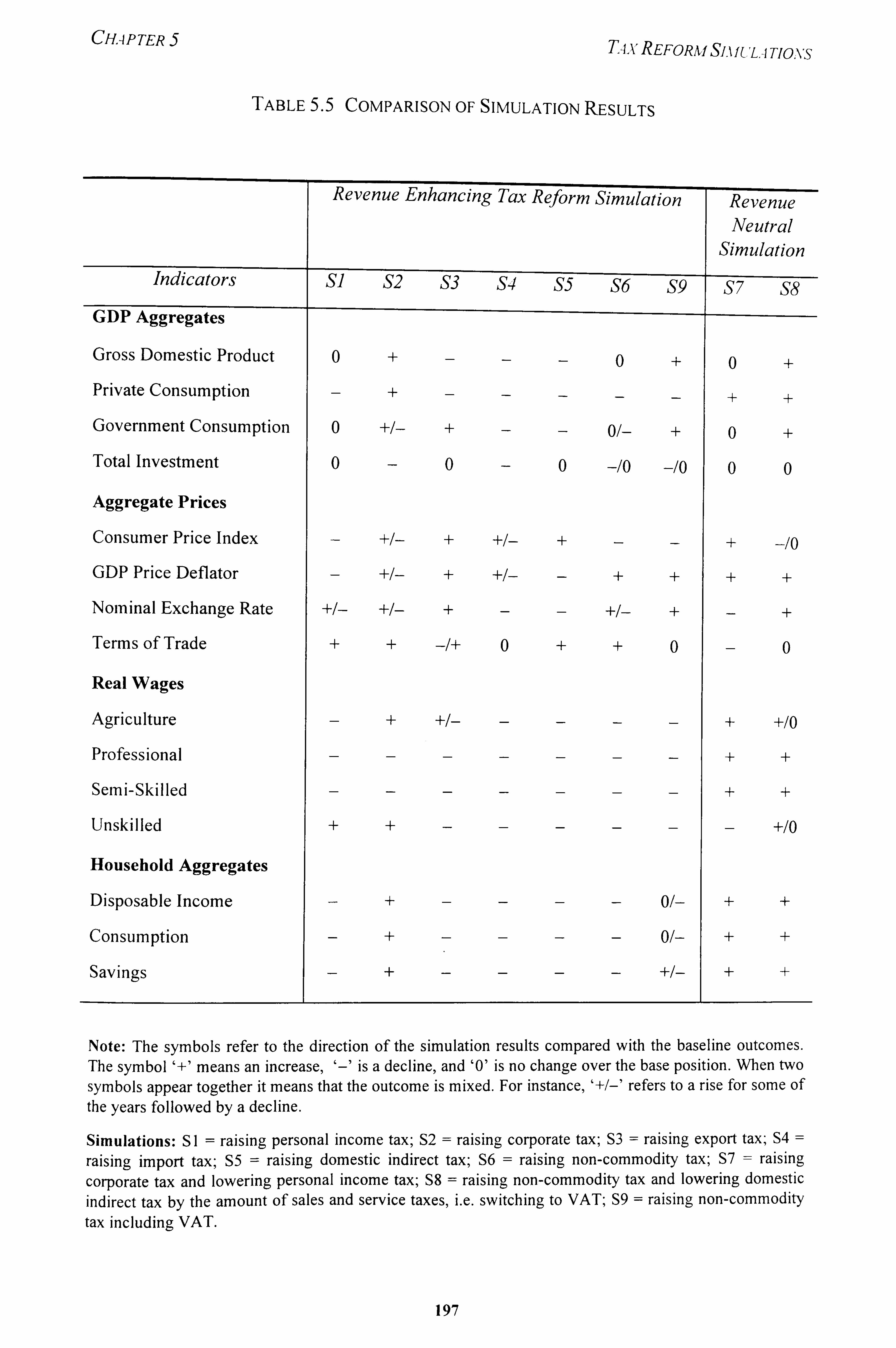
CHAPTER 5 T-I, v REFORM SIA IULA TIONS

TABLE 5.5 COMPARISON OF SIMULATION RESULTS

Indicators

GDP Aggregates

Gross Domestic Product

Private Consumption

Government Consumption

Total Investment

Aggregate Prices

Consumer Price Index

GDP Price Deflator

Nominal Exchange Rate

Terms of Trade

Real Wages

Agriculture

Professional

Serni-Skilled

Unskilled

Household Aggregates

Disposable Income

Consumption

Savings

Revenue Enhancing Tax Reform Simulation

SI S2 S3 S4 S5 S6 S9

Revenue Neutral

Simulation

S7 S8

o+---0+0+ -+-----++

o +1- +-- 0/- +0+

0-0-0 -/0 -/0 00

+/-

-+ +1- ----+ +10 -------++

-------++

++------

+10

-+---- 0/- ++

-+---- 0/- ++

+----

+/- ++

Note: The symbols refer to the direction of the simulation results compared with the baseline outcomes. The symbol '+' means an increase, '-' is a decline, and '0' is no change over the base position. When two symbols appear together it means that the outcome is mixed. For instance, '+/-' refers to a rise for some of the years followed by a decline.

Simulations: SI = raising personal income tax; S2 = raising corporate tax; S3 = raising export tax; S4

raising import tax; S5 = raising domestic indirect tax; S6 = raising non-commodity tax; S7 = raising corporate tax and lowering personal income tax; S8 = raising non-commodity tax and lowering domestic indirect tax by the amount of sales and service taxes, i. e. switching to VAT; S9 = raising non-commodity tax including VAT.

197

CHAP TER 5 TqxREFORA f SIA f ULA TIONS

Taken as a whole, if the Malaysian government intends to raise revenue from a single tax source without hurting households or negatively affecting GDP aggregates, then corporate tax (which include petroleum tax) would indeed be an ideal candidate. In fact, as shown by Simulation 2, the effect on these two aggregates can be positive. If the revenue increase were to come from more than one tax source, VATIO in combination with corporate tax would be a good way to raise revenue. Income tax can also be used for

revenue generation since it does not have a negative effect on real GDP. However , it can

have a sizeable reduction on real household disposable income and private consumption

compared with the base. The advantage of raising revenue from these three sources is

that the revenue derived from these taxes is large enough without the government having

to levy a large increase in their tax rates. For instance, to raise one percent of government

revenue in 1990 from a single tax source, the tax rates would have to be increased by 3.5

percent for corporate tax, 6.6 percent for non-commodity taxes with VAT (or VATIO),

and 8.2 percent for personal income tax. For the government to raise the same amount of

revenue from the other taxes, the tax rates would have to be increased by 36.8 percent for

export tax, 17.6 percent for import tax, 11.6 percent for domestic indirect tax, and 9.1

percent for non-commodity taxes excluding VAT.

Regarding the revenue neutral tax reforms, both the simulations S7 and S8 bring

an improvement to the household aggregates, with higher levels of disposable income,

consumption, and savings in real terms. In the case of switching from the current sales

and services taxes to VAT, there is also an improvement in the levels of GDP. Real

wages for many categories of workers are higher than the baseline position. This increase

brings an improvement to household disposable income as well as slightly higher price

levels. The two simulations indicate that there could be some economic and household

welfare gains by reforming both the direct as well as the indirect taxes in Malaysia.

In terms of policy implications, it would be useful to discuss the simulation

results in relation with the MIER Tax Reform Proposals and Bardai's (1993)

recommendations. The MIER Tax Reform Group put forward many proposals which

included the reduction of corporate tax rate, broadening the coverage of tax incentives,

reducing the top rate of personal income tax, raising the rebate given to taxpayers with

chargeable income not exceeding RM10,000, phasing out export taxes on traditional

198

CHAP TER 5 TA, v REFORA f SIA f ULA TIONS

commodities, and improving on the sales and service taxes while the adoption of a value- added type tax is being considered. Bardai argued that the corporate tax rate should not be reduced since this tax is one of the most efficient and productive tax instruments in the economy and its tax burden distribution was found to be positive. He supported the introduction of VAT system, which he said would be non-inflationary, as well as the abolition of export tax.

Our simulations support lowering income tax and adopting VAT system, both of which would be beneficial to households and the economy. We agree with Bardai that

corporate tax should not be reduced. As shown by our simulations, the increase in

corporate tax is not expected to have negative effects for real household and GDP

aggregates. In fact, there might be some benefits to be gained by raising tax revenue from

this source. Some of the actions could include rationalising the generous tax incentives

offered to corporations. There had been arguments that export tax is regressive and

should be reduced. Since the MIER tax reform proposals, duties on the export of primary

commodities had fallen, and in many cases eliminated. Arguments about the regressivity

of this tax on poor households now no longer apply as they used to. Petroleum export is

currently by far the most important contributor to export tax (over 97 percent).

8 CONCLUSION

The computable general equilibrium model is a powerful analytical tool for policy

simulation and represents a substantial advance over the earlier techniques used in

economic and development planning, such as input-output model and linear

programming model. Unlike the traditional partial equilibrium approach which relies on

ceteris paribus assumptions, CGE model enables an analyst to undertake a

comprehensive examination of a tax reform, with its complex interactions among

different sectors and agents in the macro economy.

In this chapter, we used M4, the latest CGE model developed for Malaysia, in our

counterfactual. tax reform simulations. The model was calibrated on the Malaysian 1983

Social Accounting Matrix and was subsequently updated based on more recent data from

the Malaysian National Accounts for 1990. The basic model for our tax policy reform

simulations has an essentially neo-classical model specification, with the supply-side

199

CHAPTER 5 Tqx REFOILk f SIA f ULA TIONS

driving the economy. Before performing tax simulations for the 1990s, the model was calibrated so that it produced estimates for a number of key endogenous variables that corresponded with actual development. In establishing the sectoral growth rates and the macroeconomic framework, we were guided by the Malaysian Second Outline Perspective Plan for 1991-2000. It was also necessary to reprogram the model so that more details on the various sources of government revenue and expenditure could be

obtained from the output. The model was also calibrated so that the revenue from various tax sources matched with published data for 1990-95. From 1996 onwards, we assumed that the tax indices for 1995 remained valid for the rest of the decade. Through iterative model calibrations, we arrived at a baseline simulation which replicated rather well the features and trends of the Malaysian economy and its tax structure. The baseline

simulation was then used as the standard against which we compared the outcome of the

tax reform simulations.

In the previous chapter, we discussed about how the Malaysian Government is

actively taking steps to reform its tax system, in pursuit of the objectives of economic

growth, industrial efficiency, inflation control, and improved public sector finances. This

chapter explores what the category of taxes could be raised to generate 10 percent of

government revenue, with minimal negative effects for households and the economy.

The main conclusion from the simulations is that probably the most ideal tax for this

purpose is corporate tax, which for the purpose of our estimation includes petroleum

income tax. The two other taxes that could be used in combination with corporate tax are

VATIO and possibly income tax, although the latter would have a negative effect on

household aggregates and private consumption.

The chapter also investigates if there could be some efficiency gains from

reforming the structure of direct and indirect taxes in a revenue-neutral context. For the

reform of direct taxes, we reduce personal income tax by 10 percent and calibrate the

increase in corporate taxes such that government revenue will be similar to the baseline

position. This reform will have a neutral effect on GDP aggregates but a positive effect

on households. In simulating the reform of indirect taxes, we also explore the benefits of

opting for VAT to replace the existing sales tax and service tax. The shift to value added

tax was accompanied by an improvement in real household aggregates, as well as real

200

CHAPTER T-ix REFOR, ý f S11 f ULA TIONS

GDP and private consumption. This simulation showed a slight effect in stimulating international trade, with some gain in net exports. Assuming that the implementation of

this tax is well executed, the introduction of VAT in Malaysia was not foreseen to bring

inflation. The GDP price deflator would rise by 2 percent throughout the decade which

suggests that there would be a once and for all shift in prices, without the acceleration of

price changes. This result suggests that the adoption of VAT would not be inflationary.

and this is consistent with the experience of many other countries that have adopted this

tax system.

201

Chapter 6

LABOUR SUPPLY WITH TAXATION

LITERA TURE RE VIEW

1. INTRODUCTION

This chapter and the next investigate the labour supply behaviour of household members subject to income taxation in the case of a developing country. This chapter discusses the theoretical aspects of estimating the parameters of labour supply with taxation, while the

next chapter performs an empirical analysis of labour supply with taxation on the Malaysian data set.

Labour supply has traditionally been viewed in terms of the demand for leisure.

The substitution and income effects operate together when there is a change in the wage

rates. According to theory, an increase in wage rates would increase the price of leisure

relative to the time spent at work, thereby increasing the hours of work through the

substitution effect. A wage increase would also increase the demand for leisure, which is

assumed to be a normal good, as a result of the income effect. According to

microeconomic theory, an increase in net wage resulting from tax reduction could either

reduce or increase the hours of work, depending on the relative strength of the income

and substitution effects. It will be interesting and useftil to find out whether the labour

supply response of a developing country, with socio-economic and institutional

characteristics that differ from developed countries, corresponds with the general

findings of empirical studies mainly conducted in the West.

Almost all the empirical studies on labour supply with taxation are performed for

the developed countries. Hardly any study of this nature have been conducted for the

developing countries, thereby making the study by Rochjadi and Leuthold (1994) on

Indonesia a rare exception. There are several reasons to explain the scarcity of empirical

CHAP TER 6 LITERATURE RET'IEWONLABOUR SUPPLYWITH Tqx-mov

labour supply studies with taxation in developing countries. First,, most of the available data are in aggregate form. Second, consistent with the high rates of unemployment and low wages in developing countries, the focus of many labour studies is on labour market segmentation and unemployment. Among the common themes of studies in developing

countries are labour market structure and segmentation, the unemployment and

underemployment problems, and rural-urban migration within the Arthur Lewis or Harris-Todaro frameworks. These studies usually adopt an interdisciplinary approach to

the problems of poverty, low literacy rates, high fertility and environmental deterioration.

A study on labour supply with taxation in Malaysia will, therefore, be a step in filling in

this gap in the field of knowledge.

In examining the literature on labour supply modelling, this chapter first surveys

the first and second generation studies conducted in this area, tracing the estimation

problems and the procedures adopted to overcome them. It then presents the results of

empirical studies along with some factors that could account for the wide disparity in

estimates among the two generations of studies. Next, it examines the specification of

taxes in labour supply modelling and the two common approaches used for parameters

estimation. This is followed by a discussion on the importance of taxes in affecting

labour supply based on empirical findings from studies conducted in the developed

countries. The chapter finally examines the limited empirical work done on labour supply

in developing countries, especially in Malaysia and Indonesia.

2. LITERATURE SURVEY ON STATIC LABOUR SUPPLY MODELS

2.1 First Generation Studies

There exists a large volume of empirical studies using the static labour supply models

especially in the last 30 years. I One of the important lesson that has emerged is that the

quality of empirical results is sensitive to the model specification and estimation

techniques used. Labour supply parameter estimates should in principle be based on

sound theory and careful structural analysis rather than on ad hoc models. The early

For some excellent surveys on this topic, see Heckman, Killmgsworth and MaCurdy (1981). Killingsworth (1983).

and Heckman (1993).

203

CHAPTER 6 LITERA TuRE REVIEWON LABOUR SUPPLYWITH T4x-i Tio. v

empirical studies used the ordinary least squares method (OLS), but many techniques have been developed later to overcome the inadequacy of this method in dealing with econometric problems such as selectivity, endogeneity, and errors arising from

measurement, optimisation and heterogeneous preferences in the model.

Empirical labour supply research are often divided into first and second

generation studies. The first generation empirical studies began from the 1930s to about 1974. Since the pioneering work of Schoenberg and Douglas (1937) on labour force

participation, most empirical work on labour supply have been based on the neo-classical

analysis of individual choice (Heckman, Killingsworth, and MaCurdy, 1981). Analysts

used OLS to calculate the substitution and income elasticities. The general conclusion is

that women are more sensitive than men to changes in wages and income.

A collection of first generation studies using advanced techniques on micro data

is contained in the book, Income Maintenance and Labor Supply, edited by Cain and

Watts (1973). These studies are concerned with the effects of different variables on

labour supply and the work response of non-poor groups in the population. This book,

which brings together seven research papers, 2 reflects the econometric concerns and

weaknesses of first generation work and introduces a number of econometric and

methodological innovations. The empirical findings of these studies correspond with the

other first generation research in concluding that female labour supply is more sensitive

to changes in wage rates and property income than is male labour supply. Furthermore,

leisure is a normal good for both male and female, and the compensated substitution

effect of an increase in wage will raise labour supply. Male labour supply schedule

appears to be sloping gently backwards with respect to wage, while the female schedule

is strongly positively sloped.

In their concluding chapter, Cain and Watts examine the fundamental

methodological problems faced by the studies and raised some points that set in place the

agenda for second generation research on labour supply. Since the points raised have an

2 The authors of the seven papers are: (a) Robert E. Hall, (b) Michael J. Boskin, (c) C. Russell Hill, (d) Irwin

Garfinkel, (e) David H. Greenberg and Marvin Kosters, (f) Orley Ashenfelter and James Heckman, and (g) Belton

M. Fleisher, Donald 0. Parsons and Richard D. Porter.

204

CHAP TER 6 LITERA TuRE REFIEIVON LABOUR SUPPLYWITH T4. U TION

important bearing on the direction of future studies, it may be useful to outline these issues.

I. Sample selection. Many of the studies on income-maintenance programme eliminated from the sample all groups above the poverty line. This data truncation introduces biases in the resulting estimates of income and wage effects on labour supply.

2. Choice of the dependent variable. Labour supply can be represented by either hours of work or labour participation. Both measures generate different

elasticity estimates even if the same data set is used.

3. Specification and measurement of independent variables. The problems raised include the simultaneity problem between wage and hours of work, omitted

variables (such as preference for work, personal traits, quality of education and

work experience, etc. ) that could potentially cause bias in the measure of wage

and income effects, and measurement errors in the wage variable and income

reporting.

4. Dealing with non-participants. There is the problem of how to deal with

missing wages of non-workers and their zero hours of work.

First generation studies generally ignore the underlying sources of error. The

error term is assumed to be random and the studies gave no consideration whether the

error is generated by measurement error or omitted regressors. In later studies by Burtless

and Hausman (1978), Hausman (1979) and Blomquist (1983), the model specifications

take account of some of the errors, whether they are attributable to missing variables

only, or errors in measuring hours, or both. Another problem with most first generation

studies is that they do not make clear the distinction between (a) decisions on

participation and employment, which is a dichotomous choice variable, and (b) decisions

on the number of work hours. 3 An appreciation of the participation-hours of work

dichotomy is tied up with the issue of selection bias.

3 The studies by Boskin (1973) and Kalachek and Raines (1970) are exceptions since they deal with the labour supply decision in two stages: participation and hours of work.

205

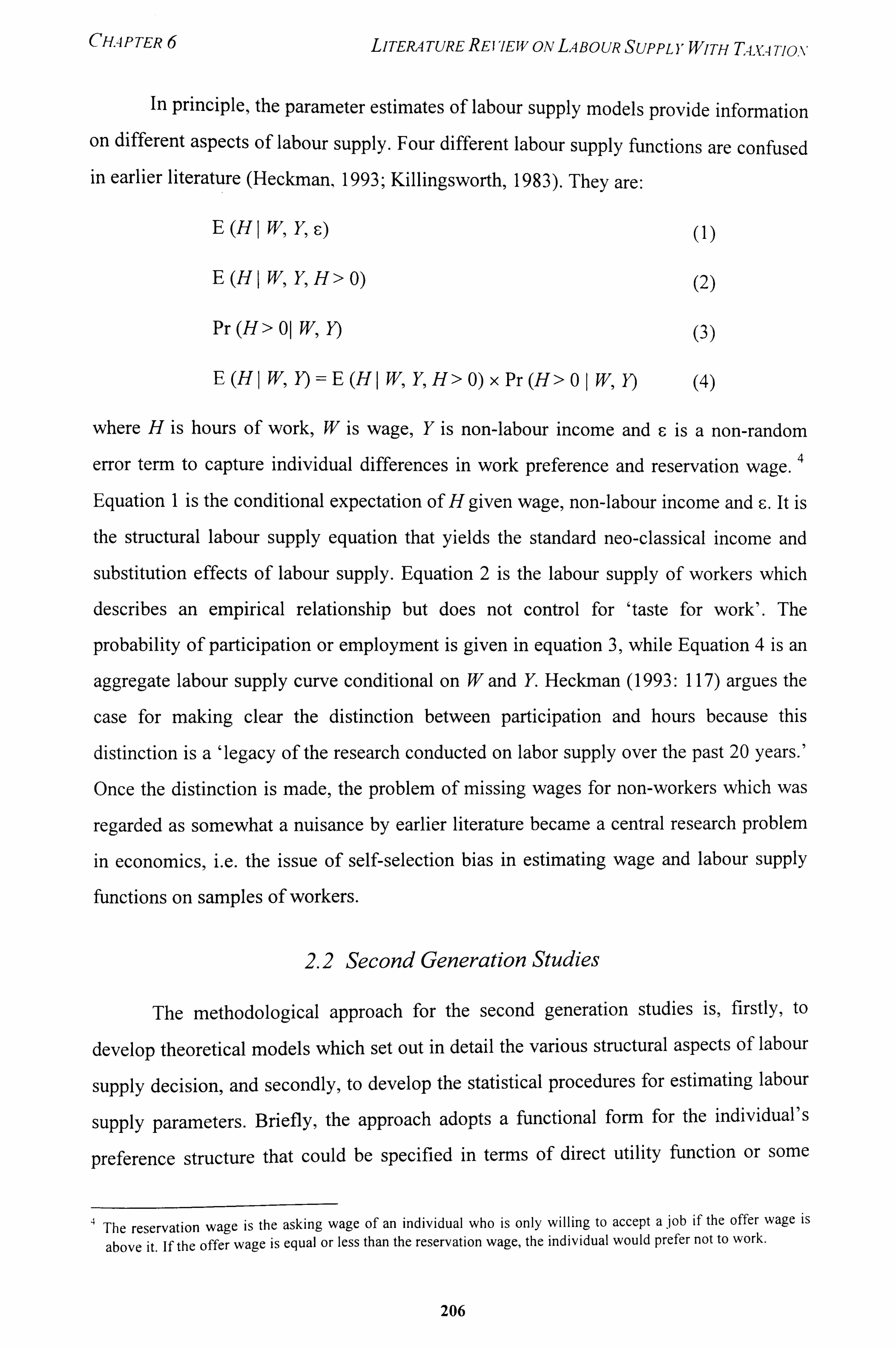
CHAP TER LITERATURE REJ 7EW ON LABOUR SUPPLYWITH T-Lu Tio. v

In principle, the parameter estimates of labour supply models provide information

on different aspects of labour supply. Four different labour supply functions are confused in earlier literature (Heckman, 1993; Killingsworth, 1983). They are:

E (H I W, Y, E: ) (1)

E(Hl W, YH>0) (2)

Pr (H> 01 W, 1)

E(Hl W, lý=E(Hl W, YH> 0) x Pr(H>O 1 W, lý (4)

where H is hours of work, W is wage, Y is non-labour income and F, is a non-random

error term to capture individual differences in work preference and reservation wage. 4

Equation I is the conditional expectation of H given wage, non-labour income and F.. It is

the structural labour supply equation that yields the standard neo-classical income and

substitution effects of labour supply. Equation 2 is the labour supply of workers which

describes an empirical relationship but does not control for 'taste for work'. The

probability of participation or employment is given in equation 3, while Equation 4 is an

aggregate labour supply curve conditional on Wand Y. Heckman (1993: 117) argues the

case for making clear the distinction between participation and hours because this

distinction is a 'legacy of the research conducted on labor supply over the past 20 years. '

Once the distinction is made, the problem of missing wages for non-workers which was

regarded as somewhat a nuisance by earlier literature became a central research problem

in economics, i. e. the issue of self-selection bias in estimating wage and labour supply

functions on samples of workers.

2.2 Second Generation Studies

The methodological approach for the second generation studies is, firstly, to

develop theoretical models which set out in detail the various structural aspects of labour

supply decision, and secondly, to develop the statistical procedures for estimating labour

supply parameters. Briefly, the approach adopts a functional form for the individual's

preference structure that could be specified in terms of direct utility function or some

4 The reservation wage is the asking wage of an individual who Is only willing to accept ajob if the offer wage is

above it. If the offer wage is equal or less than the reservation wage, the individual would prefer not to work.

206

CHAPTER 6 LITERATURE REFIEH'ONLABOUR SUPPLYWITI I TION -I Tix4

related function, such as the marginal rate of substitution or the indirect utility function. The budget line is considered specifically and the individual's utility is evaluated at each point of the budget line to obtain the point which yields the highest utility. The equilibrium can be a comer solution, interior solution, . or on a kink. The non-random error E; associated with the reservation wage and participation decision of workers and non-workers is specifically considered in the model. The term E is assumed to arise from factors known to the individual who is making the decision of whether to participate or not,, but is unknown to the analyst. The error term is also affected by the unobserved components associated with both sides of the labour supply equations, such as error in

measuring hours of work H and omitted explanatory variables.

Addressing the problem of selectivity is an innovation in second generation

research. Hours and wage data are available for workers but not for non-workers. The issue is how to treat missing wages for non-workers in parameter estimation. First

generation studies used two approaches to treat non-workers. In the first approach, non-

workers were included in the sample, with their values of H set to zero, which is

generally referred to as Procedure 1.5 This creates a misspecification problem. In the

utility maximisation model, an individual will work if his/her offer wage exceeds the

reservation wage. When this happens we observe positive number of hours. When H=0

we can only deduce that the offer wage is less or equal to the reservation wage.

Individuals have a range of reservation wage unknown to the analyst. When we include

non-workers in the sample and maximise utility by equating the marginal rate of

substitution (MRS) with real wage in our model, we are assuming that the non-workers

choose H=0 in the same way workers choose their positive values of H. This clearly

constitute a misspecification problem.

The second approach adopted in first generation work is Procedure 11 which

excludes non-workers from the sample when estimating hours of work. This gives rise to

the sample selection bias problem, which is more acute for females than males because

of the lower rate of participation among females The exclusion of non-workers results in

5 In Chapter 4 of Labor Supply, Killingsworth (1983) describes eight procedures commonly used in first generation

and second generation work on static labour supply modelling. The procedures are numbered from I to VIII.

Procedures I and 11 are used in first generation research, while the remaining six procedures, which are

econometrically more sophisticated, are used in second generation research.

207

CHAPTER 6 LITERATuRE REI'IEW OAIL, -iBoUR SUPPLYWITH T4. v4Tio, \-

the non-random selection of the error term. As a result of the censorship, wage and non- labour income variables used in the model are correlated with the error term. The

parameter estimates with the excluded non-workers will give rise to inconsistent

estimators of the total labour supply parameters. The assumption here is that the non- workers who are excluded from the estimation differ in characteristics from the workers. There are some reasons why this might be the case. Workers are those for whom the offer wage is higher than the reservation wage. This implies that workers can either attract a high market wage or they have low asking wage. Hence, workers are unlikely to be

representative of the entire population. An exception where sample selection bias is not a

problem is when everyone in the population works, say, in the case of prime-age males in

an economy with full employment.

The distinguishing feature that separates the first and second generation studies is

that the latter pays more attention to specification and estimation issues. Unlike first

generation studies, second generation work estimates the labour supply parameters by

maximising an explicit utility function subject to budget constraints. In other words, the

labour supply parameter estimates are based on microeconomic foundations rather than

on ad hoc models. 6 In addition, second generation work has also carefully distinguished

different aspects of labour supply, such as participation and hours of work. Modelling for

participation is a crucial stage in dealing with sample selection bias.

An approach to deal with sample selection bias has been introduced by Heckman

(1976,1979). This approach presents a consistent two-stage estimation method that

eliminates the specification error in the case of censored samples. It can be shown that

the conditional meanOf 6Hi 7 is as follows:

Ki = cyHki (5)

where ki = J( -Jj1uH)1[I - F( -JilaH)]. The term ki is the inverse Mill's ratio that is

obtained by performing a probit estimate on participation for all observations, workers

6 An excellent exposition on the specification of labour supply functions used in second generation research is g iven

in Stern (1986). Among the many criteria mentioned in choosing a functional form for a labour supply function are:

consistency with utility theory; convenience in estimation; ease of calculation; ease of use in applied policy

problems; facility of computation; behaviour of labour supply at low levels of work; aggregation; and flexibility in

possible response of labour to changes in the wage.

7 F-Hi is the error term associated with the heterogenous preference for work, which is assumed to be normally

distributed with mean zero and standard deviation (YH.

208

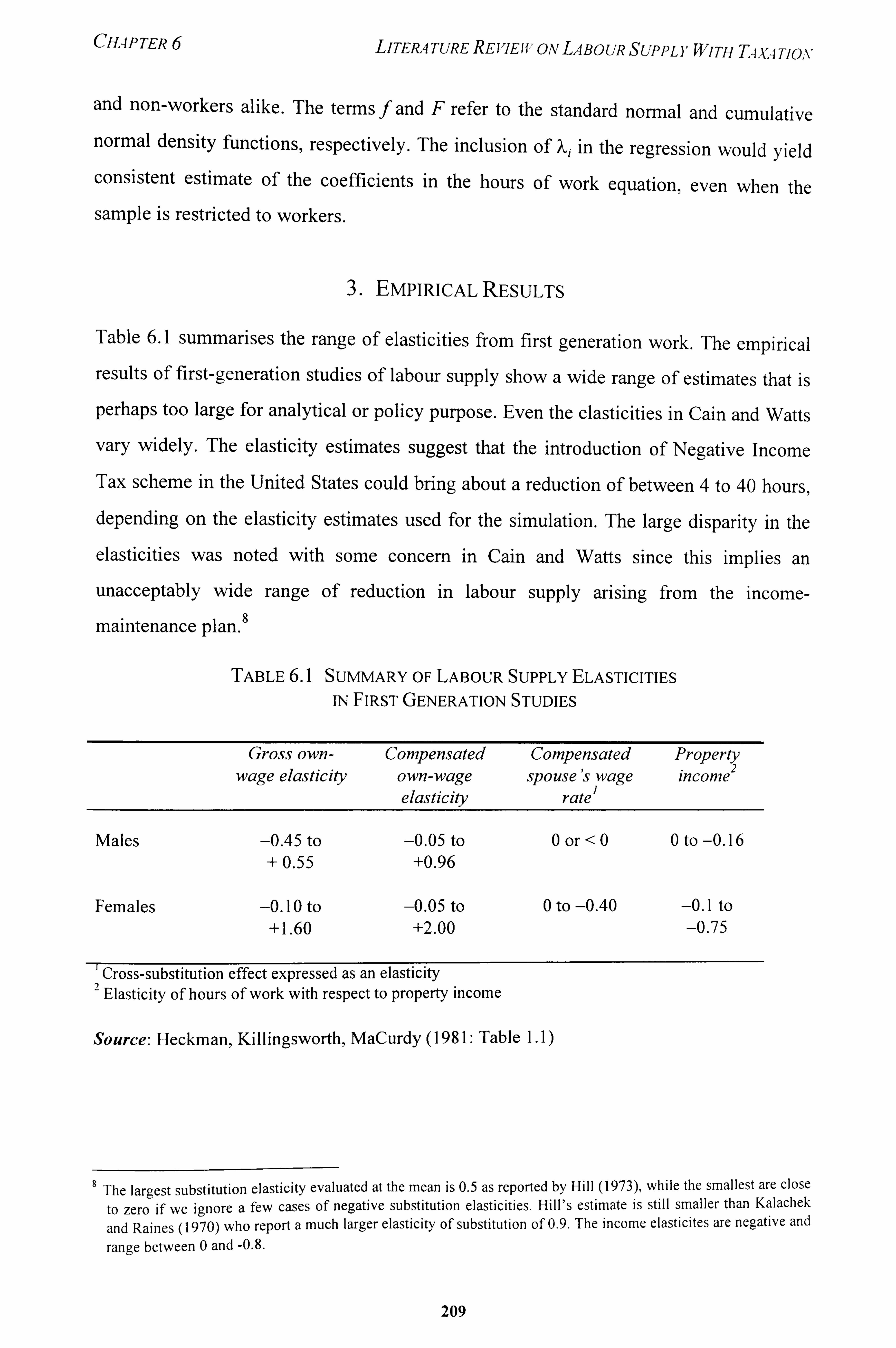
CHAPTER 6 LITERATURE REVIEIVON LABOUR SUPPLYWITH TI. V4TION

and non-workers alike. The terms f and F refer to the standard normal and cumulative normal density functions, respectively. The inclusion of ki in the regression would yield consistent estimate of the coefficients in the hours of work equation, even when the sample is restricted to workers.

3. EMPIRICAL RESULTS

Table 6.1 summarises the range of elasticities from first generation work. The empirical results of first-generation studies of labour supply show a wide range of estimates that is

perhaps too large for analytical or policy purpose. Even the elasticities in Cain and Watts

vary widely. The elasticity estimates suggest that the introduction of Negative Income

Tax scheme in the United States could bring about a reduction of between 4 to 40 hours,

depending on the elasticity estimates used for the simulation. The large disparity in the

elasticities was noted with some concern in Cain and Watts since this implies an

unacceptably wide range of reduction in labour supply arising from the income-

maintenance plan. 8

TABLE 6.1 SUMMARY OF LABOUR SUPPLY ELASTICITIES

IN FIRST GENERATION STUDIES

Gross own- Compensated Compensated Property wage elasticity own-wage spouse's wage I. ncome 2

elasticity rate I

Males -0.45 to -0.05 to 0 or <00 to -0.16 +0.55 +0.96

Females -0.10 to -0.05 to 0 to -0.40 -0.1 to +1.60 +2.00 -0.75

'Cros s- substitution effect expressed as an elasticity 2 Elasticity of hours of work with respect to property income

Source: Heckman, Killingsworth, MaCurdy (1981: Table 1.1)

8 The largest substitution elasticity evaluated at the mean is 0.5 as reported by Hill (1973), while the smallest are close

to zero if we ignore a few cases of negative substitution elasticities. Hill's estimate is still smaller than Kalachek

and Raines (1970) who report a much larger elasticity of substitution of 0.9. The income elasticites are negative and

range between 0 and -0-8.

209

CHAP TER 6 LITERA TuRE RE FIE I VON LA BO UR SUPPLY WITH T4X4 TION

Despite methodological improvements in the second generation procedures, they

do not manage to narrow the range of elasticity estimates. q There were more studies on female labour supply in second-generation studies than on male labour supply. The few

studies on male labour supply indicate that male labour'supply is less sensitive to wage rates and property income than female labour supply. According to Killingsworth (1983),

most of the second- generation studies imply that the gross wage elasticities range between -0.20 and +0.14 for males and -0.32 to +15.0 for females. The compensated

wage elasticities range from -0.06 to +1.00 for males and from -1.06 to +14.79 for

females. However,, Killingsworth argues that when studies with negative compensated

elasticities are discarded, this narrows the range of uncompensated elasticities for U. S.

men to -0.03 to 0.14. The anomaly to these findings is the results reported by Nakamura,

Nakamura, and Cullen (1979, for Canadian women) and Nakamura and Nakamura (198 1,

for both Canadian and US women). Their results depart from the other first- and second-

generation research by showing that the uncompensated wage elasticities for female

hours of work are negative.

It has been argued that differences in estimation method, functional form and data

base of the various studies account for the wide heterogeneity of elasticity estimates. In

the seventies and eighties, there were some studies using a similar data set to test the

sensitivity of different estimation procedures and assumptions. DaVanzo, DeTray and

Greenberg (1973) applied many different procedures to the 1976 Survey of Economic

Opportunity (SEO) data set in the United States. Another sensitivity study was

performed by Masters and Garfinkel (1977) who pursued the same research question

using the data from the 1967 SEO and the 1972 Michigan Panel Study of Income

Dynamics (PSID). The two studies conclude that the wide diversity of results are the

outcome of some of the following factors: ' 0

1. Problems in measuring the hours and wage rate variables. Several definitions

of hours worked have been used in different studies. Since hours worked is

often used in calculating the wage rate, errors in measuring true hours worked

9 For a listing of the estimates of structural elasticities derived in second-generation research, see Table 4.3 in

Killingsworth (1983).

10 Pencavel (1986) and Fallon and Verry (1988: 60-64) provide some elaboration on the problems of measurement

and definitions of variables.

210

CHAPTER 6 LITERA TuRE REI 7EW ON LABOUR SUPPLYWITH T, 4,, V4 Tlo, %,

induce a spurious negative correlation between the two variables. In tax analysis, the tax liability used to calculate net wage is based on official income tax schedule which is unlikely to conform to the actual tax paid by the individual since the analyst does not know the exact amount of tax deductions

and the extent of tax avoidance and tax evasion in the system.

2. Difficulty in measuring non-wage income accurately. Different procedures are used in the calculation of non-wage income that give rise to the wide range of non-wage income effects estimated in the various models. It is not uncommon for studies to report a positive association between non-wage income and hours of work. Of the 57 different estimated coefficients on non-wage income

reported in DaVanzo, DeTray and Greenberg, only 16 are significant; of these,, half of the estimates have positive signs while the other half negative

signs.

3. Effect of other explanatory variables. Some of the explanatory variables used in the models include age, education, work experience, family size and

structure, region, job satisfaction, state of health, etc. DaVanzo et al. found

that the size and signs of the wage coefficient are extremely sensitive to the

presence of years of schooling. Studies that include education and number of

dependants as the explanatory variables for the hours of work equation show a

significant positive relation relationship between these variables and hours of

work.

In the eighties, an influential sensitivity analysis was undertaken by Thomas

Mroz (1987) on the 1976 Panel Study of. Income Dynamics data set. Using a sample

consisting of 753 white married women aged 30-60, he conducted a detailed sensitivity

analyses using the alternative first- and second-generation estimation methods. His

simulation exercises show the sensitivity of elasticity estimates to the choice of

instruments and endogeneity assumptions.

As a baseline approach, Mroz uses OLS to estimate the hours equation on a

sample of those who work (428 women in the sample were working in 1975). This

approach is often used in first generation work and is referred to as Procedure 11 by

211

CHAPTER 6 LITERATURE REVIEff" ONLABOUR SUPPLY WITH T4, VATIOX

Killingsworth. This procedure yields negative elasticities for both the uncompensated wage effect (-0.0113) and income effect (-0.0028), while the inclusion of the variable children under age six reduces hours of work substantially. It was pointed out that a negative wage effect can arise if there is a random measurement error in hours of work which causes a spurious negative relationship between hours of work and wages. As a variant to Procedure II, Mroz uses the women's labour market experience' I as an instrumental variable for wage, which is regarded an endogenous variable. By using the two stage least squares (2SLS) method, the estimate for the uncompensated wage response becomes positive and significant, while the income effect is negative and large. By excluding the experience variable as an instrument, the uncompensated wage elasticity and the income elasticity decrease in size while still retaining their signs. Mroz

performs exogeneity tests for experience, children and non-wage income and concludes that labour market experience is not exogenous in the labour supply equation. He, however, cannot reject the exogeneity of children and non-wage income.

The procedure 11 described above is based on a subsample of working women and does not control for self-selection bias. To examine the importance of self-selection bias, Mroz uses the Heckit multistage approach or Procedure VIII. He calculates the inverse Mills ratio k from the probit model. The wage variable is instrumented and used in the 2SLS estimation of the hours worked equation. The regression yields a small positive

uncompensated wage effect and a small positive income effect. The statistics are

significant when labour market experience are excluded from the model but are insignificant with the inclusion of experience. Mroz concludes that the estimated

uncompensated wage effect is positive but very small and the income effect is negative

and small. This result also challenges the conventional wisdom that the wage and income

elasticities for women are larger than of men and, therefore, concurs with Nakamura and

Nakamura (19 8 1).

The measure of labour market experience used in this study is the number of years the woman worked for money

since her eighteenth birthday. Mroz (1987: 774) argues that women who have worked many years in the past tend

to have higher wages and work more hours in the present. The number of years worked between two women

reflects a systematic difference in the unobservables influencing their labour supplies (e. g. 'tastes for work'), which

makes women's labour market experience endogenous to the labour supply function.

212

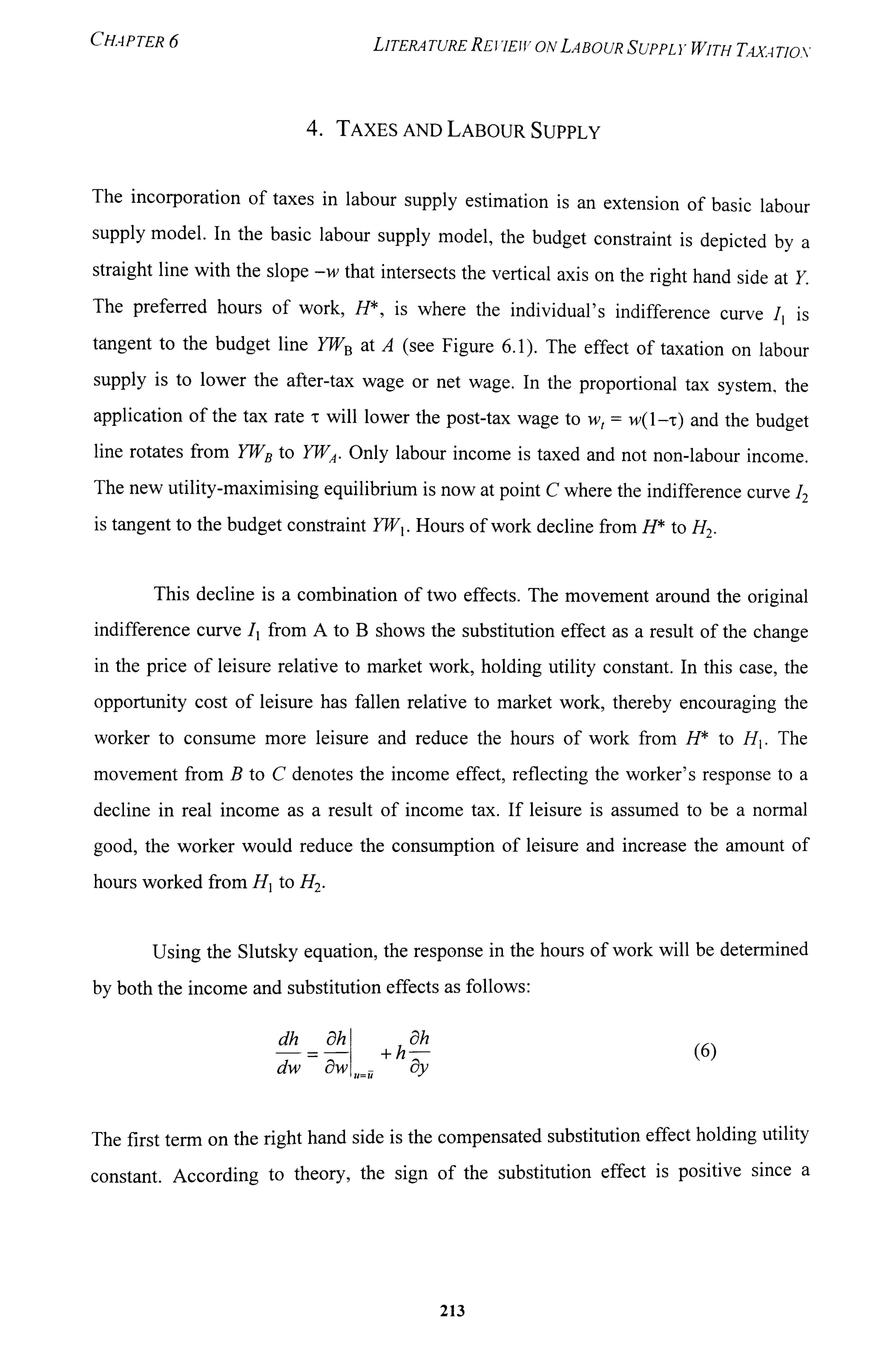
CHAPTER 6 LITERATURE REFIEIVONLABOUR SUPPLYWITH TAXATION

4. TAXES AND LABOUR SUPPLY

The incorporation of taxes in labour supply estimation is an extension of basic labour

supply model. In the basic labour supply model, the budget constraint is depicted by a straight line with the slope -w that intersects the vertical axis on the right hand side at Y. The preferred hours of work, H*, is where the individual's indifference curve 11 is

tangent to the budget line YWB at A (see Figure 6.1). The effect of taxation on labour

supply is to lower the after-tax wage or net wage. In the proportional tax system, the

application of the tax rate r will lower the post-tax wage to w, = w(I-T) and the budget

line rotates from YWB to YWA. Only labour income is taxed and not non-labour income.

The new utility-maximi sing equilibrium is now at point C where the indifference curveI2 is tangent to the budget constraint YWI. Hours of work decline from H* to H2.

This decline is a combination of two effects. The movement around the original indifference curve I, from A to B shows the substitution effect as a result of the change in the price of leisure relative to market work, holding utility constant. In this case, the

opportunity cost of leisure has fallen relative to market work, thereby encouraging the

worker to consume more leisure and reduce the hours of work from H* to H1. The

movement from B to C denotes the income effect, reflecting the worker's response to a

decline in real income as a result of income tax. If leisure is assumed to be a normal

good, the worker would reduce the consumption of leisure and increase the amount of

hours worked from H, to H2.

Using the Slutsky equation, the response in the hours of work will be determined

by both the income and substitution effects as follows:

A c9h h ah

dw aw u=i4-

ay (6)

The first term on the right hand side is the compensated substitution effect holding utility

constant. According to theory, the sign of the substitution effect is positive since a

213

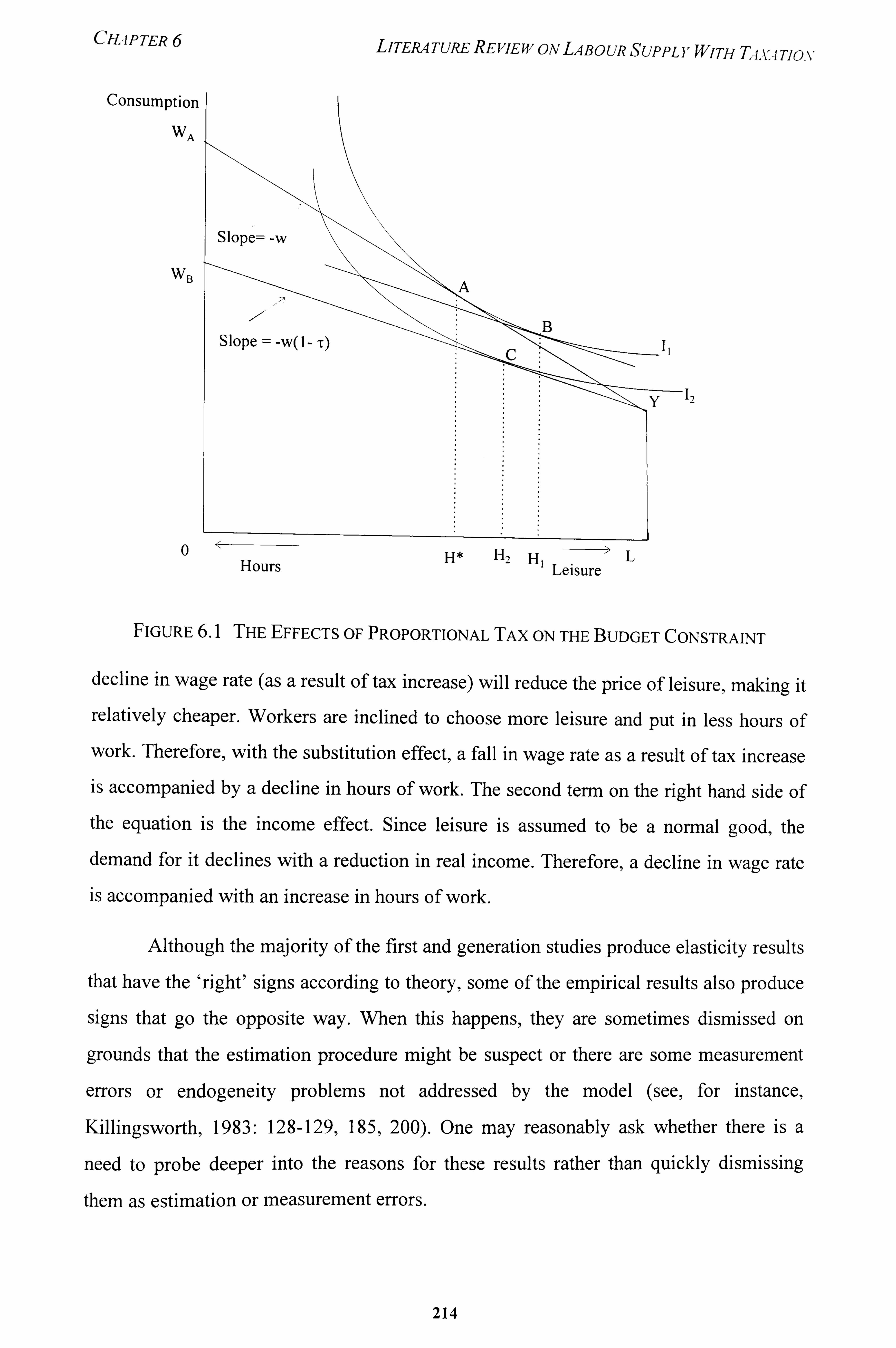
CHAPTER

Consumption

WA

WB

LITERATuRE REVIEW ONLABOUR SUPPLYWITH T4. V-ITIO. \,

12

0

FIGURE 6.1 THE EFFECTS OF PROPORTIONAL TAX ON THE BUDGET CONSTRAINT

decline in wage rate (as a result of tax increase) will reduce the price of leisure, making it

relatively cheaper. Workers are inclined to choose more leisure and put in less hours of work. Therefore, with the substitution effect, a fall in wage rate as a result of tax increase

is accompanied by a decline in hours of work. The second term on the right hand side of the equation is the income effect. Since leisure is assumed to be a normal good, the demand for it declines with a reduction in real income. Therefore, a decline in wage rate is accompanied with an increase in hours of work.

Although the majority of the first and generation studies produce elasticity results

that have the 'right' signs according to theory, some of the empirical results also produce

signs that go the opposite way. When this happens, they are sometimes dismissed on

grounds that the estimation procedure might be suspect or there are some measurement

errors or endogeneity problems not addressed by the model (see, for instance,

Killingsworth, 1983: 128-129,185,200). One may reasonably ask whether there is a

need to probe deeper into the reasons for these results rather than quickly dismissing

them as estimation or measurement errors.

214

H* H2 H -----> L Hours ' Leisure

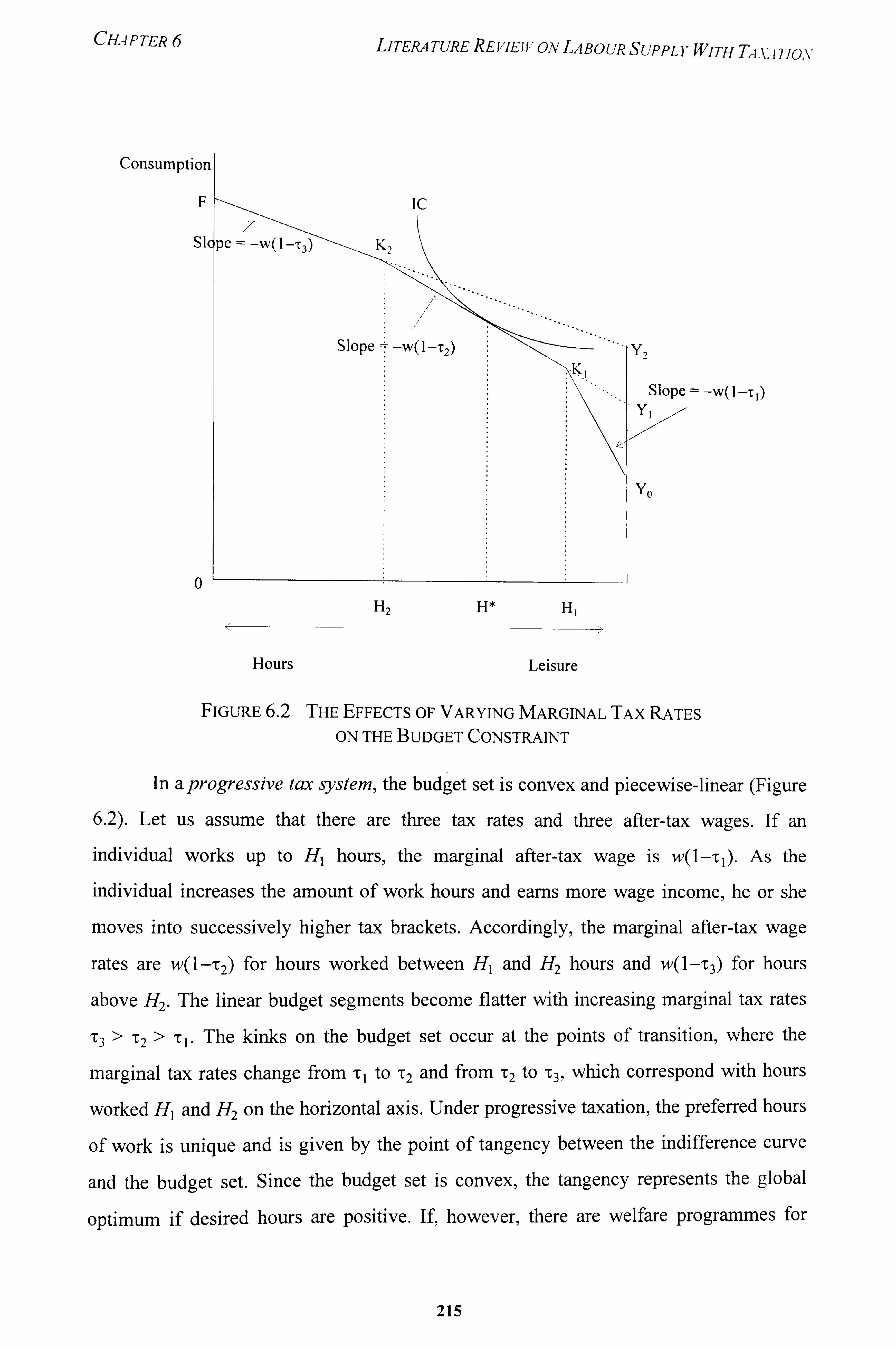
CHAPTER

Consumptiot

F

sl

LITERATURE REVIEIVON LABOUR SUPPLYWITH TAV. 4 Tlo, %'

= -W(l -T 1)

0 H2 H* H,

Hours Leisure

FIGURE 6.2 THE EFFECTS OF VARYING MARGINAL TAx RATES ON THE BUDGET CONSTRAINT

In a progressive tax system, the budget set is convex and piecewise-linear (Figure

6-2). Let us assume that there are three tax rates and three after-tax wages. If an

individual works up to H, hours, the marginal after-tax wage is w(I-CI). As the

individual increases the amount of work hours and earns more wage income, he or she

moves into successively higher tax brackets. Accordingly, the marginal after-tax wage

rates areWO _T2) for hours worked between H, and H2 hours andWO _T3) for hours

above H2. The linear budget segments become flatter with increasing marginal tax rates

'C3 > 'C2 > T1. The kinks on the budget set occur at the points of transition, where the

marginal tax rates change fromr, to T2 and fromT2 to T3. which correspond with hours

worked H, and H2on the horizontal axis. Under progressive taxation, the preferred hours

of work is unique and is given by the point of tangency between the indifference curve

and the budget set. Since the budget set is convex, the tangency represents the global

optimum if desired hours are positive. If, however, there are welfare programmes for

215

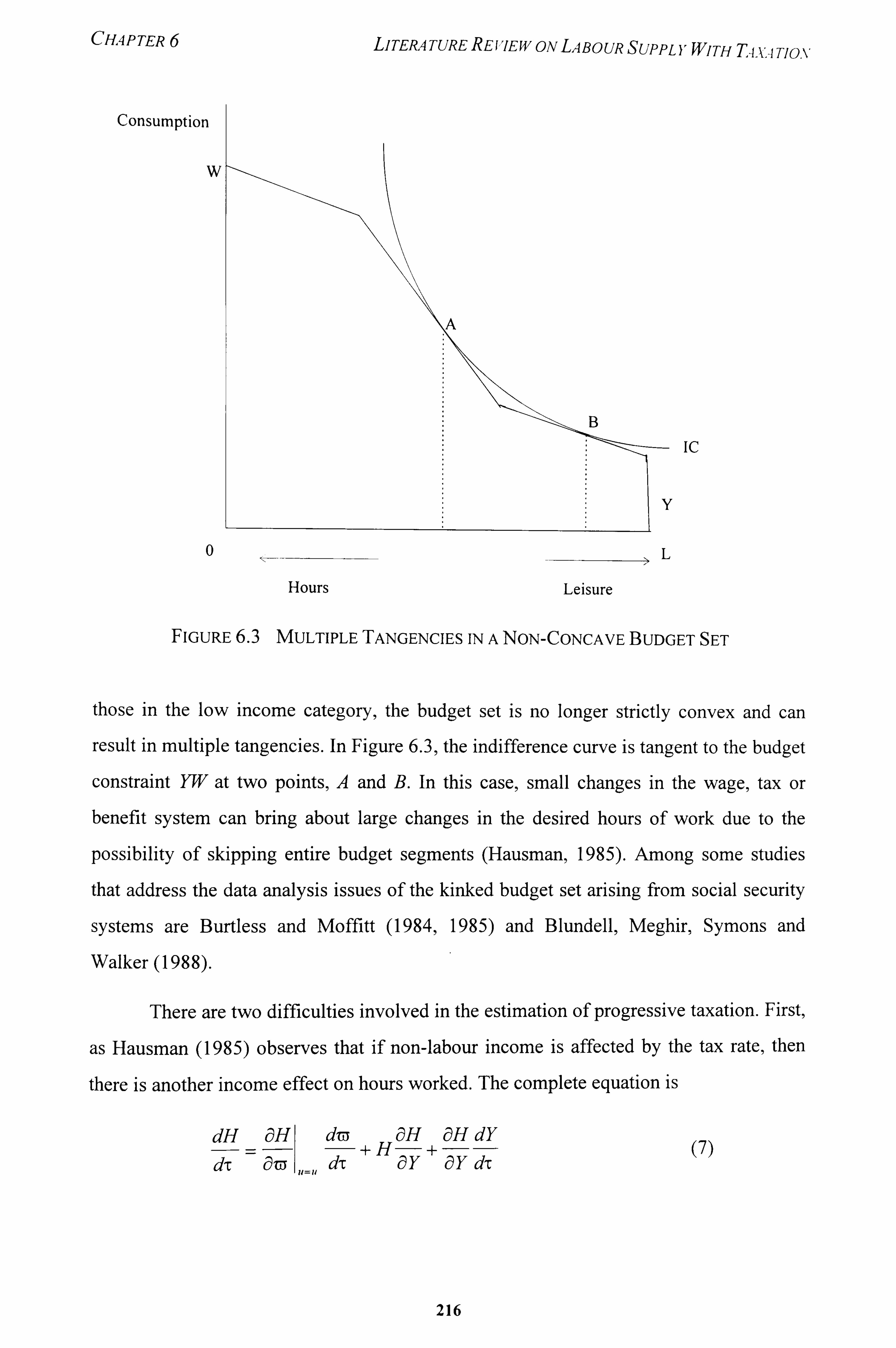
CHAPTER

Consumption

w

0

LITERATUREREVIEW ON LABOUR SUPPL YWITH T4-k, '-ITlo, %-

Hours Leisure

ic

FIGURE 6.3 MULTIPLE TANGENCIES IN A NON-CONCAVE BUDGET SET

those in the low income category, the budget set is no longer strictly convex and can

result in multiple tangencies. In Figure 6.3, the indifference curve is tangent to the budget

constraint YW at two points, A and B. In this case, small changes in the wage, tax or

benefit system can bring about large changes in the desired hours of work due to the

possibility of skipping entire budget segments (Hausman, 1985). Among some studies

that address the data analysis issues of the kinked budget set arising from social security

systems are Burtless and Moffitt (1984,1985) and Blundell, Meghir, Symons and

Walker (198 8).

There are two difficulties involved in the estimation of progressive taxation. First,

as Hausman (1985) observes that if non-labour income is affected by the tax rate, then

there is another income effect on hours worked. The complete equation is

dH =

aH dm +H

aH +

aH dY d-c d-c aY aY d-c

(7)

216

>1

CHAPTER 6 LITERATURE REFIEWON LABOUR SUPPLYWITH T-i. k, 4TIO. \'

where H is hours worked, -c is marginal tax rate, m is net wage after tax, and Y is non- labour income. This implies that in estimating the effect of taxes on labour supply in a progressive tax system, the income and substitution effects of the changes in both wage and income should be considered.

The difficulty involved in the estimation of progressive taxation is finding the

point of tangency on a curved budget set. Under progressive taxation, the budget set is

convex and a global optimum can be found as a comer solution, at a budget segment or

even at one of the kinks. Moffitt (1990) provides a good discussion of some methods that

could be used in estimating a non-linear budget set. There are two common approaches have been used in the literature used for analysing labour supply with taxation. First, is

the Piecewise-Linear Budget Constraint approach that had been used in studies such as Burtless and Hausman (1978), Wales and Woodland (1979), Flood and MaCurdy (1992),

and Blomquist (1996). The second approach is the Instrumental Variable method that is

used in Boskin (1973), Hall (1973), Mroz (1987), Flood and MaCurdy (1992) and

Blomquist (1996). However, before elaborating on the two commonly used approaches,

it will be useful to explain the concept and derivation of the 'virtual income', a device

that is used by both approaches to overcome the difficulty of finding the maximum on a

convex budget set.

Virtual income refers to the proxy non-labour income that results from extending

a given budget segment to the vertical axis on the right hand side. This device is used by

analysts during the last two decades ranging from Rosen (1976), Hausman (198 1 a) to

Flood and MaCurdy (1992) and Blomquist (1996). The intersection of the extended

linear budget segment with the vertical axis gives the level of virtual income. It is the

assumed level of property income that corresponds with the marginal wage rate

applicable to the individual. In Figure 6.2, the virtual income corresponding with the

marginal tax rates 'r2and'13 are Y, and Y2, respectively.

4.1 Piecewise-Linear Budget Constraint Approach

Sometimes dubbed the Hausman Method, this approach was used by Burtless and

Hausman (1978) to study the labour supply effects of a negative income tax and the

federal income which creates a budget constraint that is not strictly convex. Hausman

217

CHAPTER 6 LITERA TuRE REI, 7EJJ'ON LABOUR SUPPL YWITH TA, k, A TION

(1979,198 1 a) provide details on this approach which are further elaborated by Blomquist

(1983), Moffitt (1990), and Flood and MaCurdy (1992). The econometric estimation

allows for two error terms. The first error term is to represent unobserved heterogeneity

of preferences since different individuals will choose to work different amount of hours

even if they face the same budget constraint. The second error term represents

optimisation error which arises because individuals cannot choose their hours of work

precisely even if they wish to locate at a particular point on the budget constraint. Although measurement error is conceptually different from optimisation error, this model does not make an econometric distinction between the two types of errors.

To illustrate the model, let H be hours of work, W(l --c 1) andWO -'C2) be the net

wage on segments I and 2, T, and T2 are the corresponding marginal tax rates, yj and Y2

are the intercepts or virtual income for the first and second segments, and H* hours of

work be the kink. Let u be the heterogeneity error term and 6 be the optimisation error.

The equations describing the hours of work an individual would have under each of the

three possible locations which would maximise his or her utility are as follows:

(x +ßW(I-T1) + yyl +U+E if utility is max. on segment I

H= cc +P WO -T2) +7Y2 + ý) +6

H=H*+c

if utility is max. On segment 2

if utility is max. on the kink

The equations that describe the choice of segment or kink that would maximise utility are

as follows:

Segment I if (x + PW(I--cl) + 7y, +< H* (8)

Segment 2 if (X + PWO-T2) + 7Y2 +> H* (9)

Kink if a+ PW(I-, rl) + 7y, +u> H* (10)

and (X + Pw(l-T2) + YY2 + 1) < H*

The distributIon of the error terms are assumed to be normal and the studies using

this approach estimate the equation coefficients by maximum likelihood. The parameters

are estimated using an iterative algorithm. First, the estimation procedure checks if utility

is maximised by a comer solution where H= HO. If it is not, the procedure checks

218

CHAPTER 6 LITERA TuRE RET 7ETJ, 'ON LABOUR SUPPL YWITH T4., u7-J0, V

whether the maximum lies on the first segment where desired hours is less than H*. If this is not the case, then the procedure checks whether the maximum lies on the second segment where desired hours is greater than H*. Hence, individuals with lower values of u would choose the first segment and individuals with higher values of U would choose the second segment. If utility is not maximised at the two segments, the maximum is assumed to lie on the kink where u falls between the high and low values. This iterative

method searches all possible parameter values that would maximise utility for all observations in the sample.

The model can be estimated with only one error term. In studying the effect on income tax on labour supply, Wales and Woodland (1979) estimate the model with

optimisation error F- but do not include the heterogeneity error u, which suggests that

individuals with the same budget constraint are maximising at the same points. Some

other studies such as Hausman (1980), Zabalza, Pissarides and Barton (1980), and

Moffitt and Nicholson (1982) adopted the model which includes the heterogeneity error

but not the optimisation error. The assumption here is that individuals could locate at the

kink points without any error. As Moffitt (1990: 136) observes, the implication of the

model with the optimisation error is that the observed segment location for an individual

need not necessary be the location where he or she maximises utility.

When the tax system is not strictly progressive, especially in the presence of

government transfer programmes, the analysis becomes more complicated because the

budget set is no longer convex. This gives rise to the possibility of multiple tangencies

between the indifference curves at the budget set. Hausman (1985) describes how the

estimation can be done. The labour supply function can be derived from the indirect

utility function by using Roy's identity. The global optimum can be found by comparing

all feasible tangencies and the tangency with highest utility is chosen as the preferred

hours of work. Either the non-linear least squares or a Tobit procedure could be used to

estimate the unknown coefficients, as with the case of the convex budget set.

The Hausman method provides an elegant solution to the parameter estimation of

the labour supply function. It takes into account the linear segments and kinks on the

after-tax budget set as well as admits randomness in hours of work arising from both the

measurement error and the variation in individual preference. It also takes into account

219

CHAPTER 6 LITERA TuRE REVIEW ON LABOUR SUPPLYWITH T4, u Tiox

the endogeneity of the marginal tax rate in estimation. However, there are some shortcomings that can affect the reliability of the estimates. The empirical studies of male labour supply using the Hausman approach tend to Produce higher substitution and lower income effects than empirical work based on other approaches, thereby producing larger estimates of both labour-supply responses and dead-weight losses associated with the progressivity of taxation (Heckman, 1983; MaCurdy et al., 1990).

The Hausman method assumes that there is perfect knowledge on the part of the analyst and the individual with regard to the entire budget constraint. The assumption is that the analyst is able to observe perfectly the wage and income variables and the model makes no allowance for errors in measuring the budget constraint. This assumption is

most likely to be violated in empirical analysis. The true budget set is not known to the

econometrician because of measurement errors, including those made in tax

computations as a result of unobserved variability in deductions and exemptions. Without full accounting of the variability, Heckman (1983: 73-74) argues that the

piecewise-linear budget constraint procedure does not produce consistent estimates and

may be less robust than the earlier instrumental variable estimation procedures of Boskin

(1973) and Hall (1973).

In addition, the Hausman method makes very strong exogeneity assumptions in

presuming that all variables, including gross wages and non-labour income, used in the

calculation of taxes are exogenous determinants of labour supply behaviour. Some

authors such as Da Vanzo, De Tray and Greenberg (1976), Pencavel (1986), and Flood

and MaCurdy (1992) argue that wages and income are endogenous variables. If this is

the case, the substitution and income effects obtained from this method may not be

dependable.

Finally, a major problem with this approach is the parametric restriction adopted

that constraints the signs of the substitution and income effects. MaCurdy, Green, and

Paarsch (1990) observe that requiring the Slutsky condition to hold at various points is

not based on economic theory but, in the case of this procedure, on the need to obtain a

properly defined statistical model. This inequality restrictions must hold in order for the

likelihood functions, which are used in deriving the maximum on the linear segments of

220

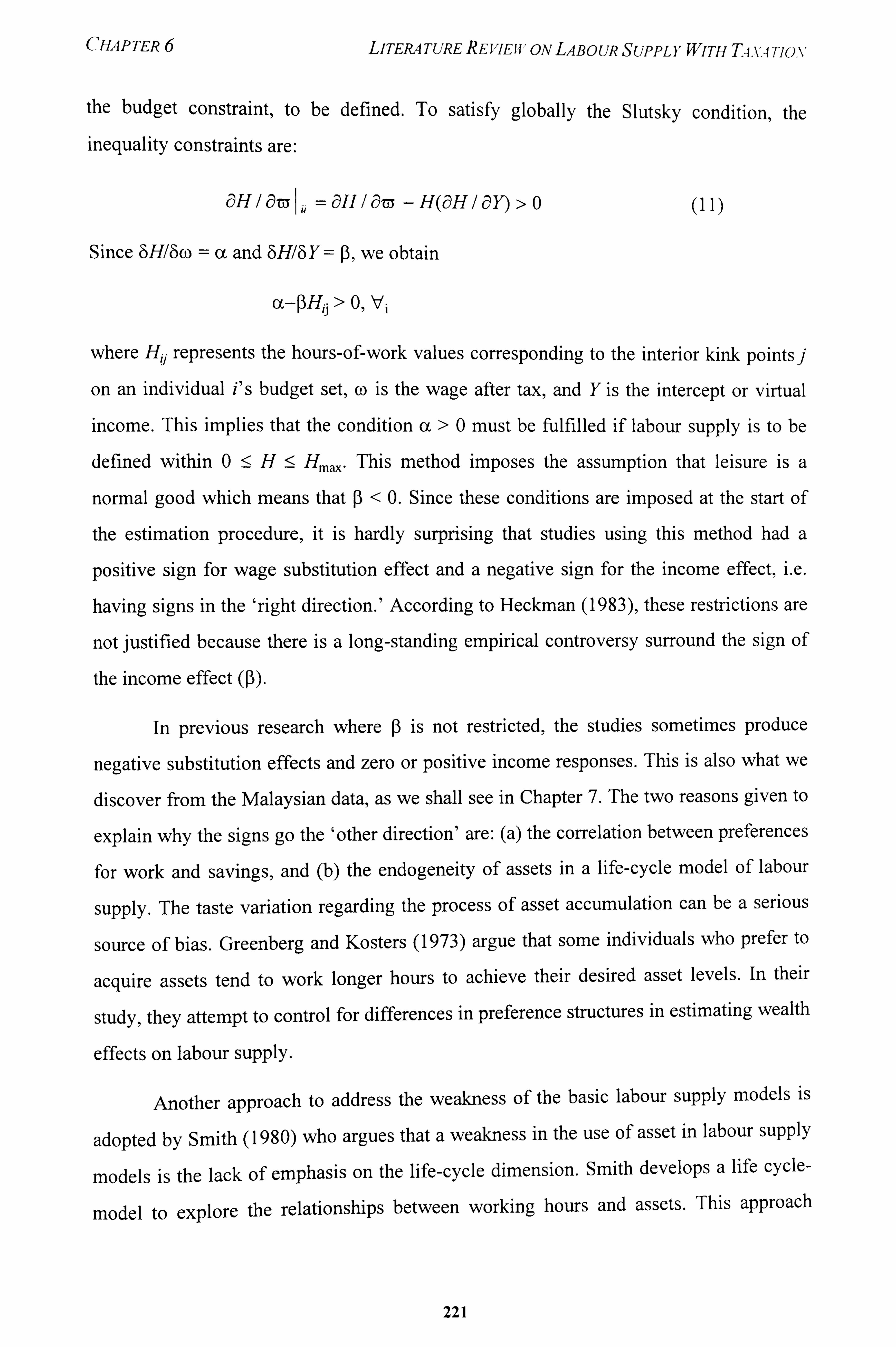
CHAP TER 6 LITERATURE REVIEWON LABOUR SUPPLYWITH TA. vmox

the budget constraint, to be defined. To satisfy globally the Slutsky condition, the inequality constraints are:

alllaoll, =aHlam -H(aHlan>O (11)

Since 6H/6o) = cc and 8H16 Y=P, we obtain

(x-ßHij > 0, Vi

where Hy. represents the hours-of-work values corresponding to the interior kink points j

on an individual i's budget set, (o is the wage after tax, and Y is the intercept or virtual

income. This implies that the condition (x >0 must be fulfilled if labour supply is to be

defined within 0 :! ý- H : ý- Hma, This method imposes the assumption that leisure is a

normal good which means that P<0. Since these conditions are imposed at the start of

the estimation procedure, it is hardly surprising that studies using this method had a

positive sign for wage substitution effect and a negative sign for the income effect, i. e.

having signs in the 'right direction. ' According to Heckman (1983), these restrictions are

not justified because there is a long-standing empirical controversy surround the sign of

the income effect (P).

In previous research where P is not restricted, the studies sometimes produce

negative substitution effects and zero or positive income responses. This is also what we

discover from the Malaysian data, as we shall see in Chapter 7. The two reasons given to

explain why the signs go the 'other direction' are: (a) the correlation between preferences

for work and savings, and (b) the endogeneity of assets in a life-cycle model of labour

supply. The taste variation regarding the process of asset accumulation can be a serious

source of bias. Greenberg and Kosters (1973) argue that some individuals who prefer to

acquire assets tend to work longer hours to achieve their desired asset levels. In their

study, they attempt to control for differences in preference structures in estimating wealth

effects on labour supply.

Another approach to address the weakness of the basic labour supply models is

adopted by Smith (1980) who argues that a weakness in the use of asset in labour supply

models is the lack of emphasis on the life-cycle dimension. Smith develops a life cycle-

model to explore the relationships between working hours and assets. This approach

221

CHAP TER 6 LITERATURE REl'IEW ON LABOUR SUPPLYWITH T4. u Tjox

shows that both the variables are simultaneously determined by similar economic forces, and the correlation between them should not be interpreted as evidence of a causal sequence from assets to market work. As Smith argues, the standard practice of using assets to measure wealth effects on the demand for leisure is theoretically inappropriate since it overlooks or lack emphasis on the life-cycle approach. They have to be considered in a multiperiod model instead of being forced into the confines of a one- period model.

4.2 Instrumental Variable Approach

This is another method that is often used in labour supply studies. In the past,

analysts had tried to estimate the labour supply parameters by linearising the budget

constraint around the optimum point and used net wage and virtual income as independent variables in the Ordinary Least Squares (OLS) procedure. However, using OLS on the linearised model will generate inconsistent estimates as a result of either heterogeneous preferences or measurement/optimisation errors or both. In first

generation research, OLS is applied to the labour supply function

Hi = g(Wi, Vi) + Fi

where Hi is the individual's observed quantity demanded, Wi is the individual's wage, V,

is the individual's virtual income for that segment, and ci is the error term. This approach

can give rise to biases because of the problems of endogeneity and reverse causality. The

right-hand side variables for wage and virtual income are endogenous because they are

partly determined by the individual when he or she makes the choice of labour supply. In

other words, wage and virtual income are partly determined by hours of work. Hence, the

causality runs from the choice of hours to the choice of wage and virtual income, rather

than the other way round. This approach does not take into account the problem of

individuals locating at the kinks, which can be a problem if there is the tendency of

workers to do this as a way of reducing their tax burden.

To get around the reverse causality problem, the instrumental variables

techniques have been used in studies that have linearised the slope and used it along with

the intercept as independent variables in the regression equation. The method is

222

CHAPTER 6 LITERA TuRE REVIEW ON LABOUR SUPPLYWITH T4-v. 4 Tjox

essentially to construct an instrumental variable that is correlated with the endogenous regressor variable but, uncorrelated with the error term. In this case, the analyst tries to develop instrumental variables for the wage and virtual income variables that are exogenous but are uncorrelated with the error term. Thi's approach is equivalent to the technique used in getting around the simultaneous equation problem where there is a two-way relationship between the variables on the left- and right-hand side of the regression equation and where the right-hand side variable is correlated with the error term. The choice of instrument set varies across studies which adopt different

assumptions on exogeneity.

Among the first attempts to use the instrumental variable approach are Boskin

(1973) and Hall (1973). In cross section studies, the observed wage, W, may differ from

the true wage, Wi*, by a random error of measurement, u. In addition, the wage rate is

often calculated by dividing total earnings on hours of work. This implies that errors in

measuring hours of work are transmitted to the wage variable which will be related to the

error term, giving rise to biased, even inconsistent, estimate of P. To overcome this

problem of wage measurement, Boskin and Hall use the instrumental variable estimator,

which is expressed in terms of observable personal characteristics.

A different approach is adopted in Rosen's (1976) study on the effect of the

federal income tax and Hausman and Wise's (1976) study on the effect of a negative

income tax. The marginal tax rate was evaluated at the same level of hours of work (i. e.

at 40 hours per week) for all individuals in order to construct net wage rates and virtual

incomes. The rationale for this procedure is that since the net wage variable is not

constructed on the basis of actual, chosen hours of work, it is uncorrelated with the error

term in the labour supply equation. This approach faces the problem of partly

misrepresenting the actual tax rate faced by individuals who do not work at 40 hours per

week.

There is yet another problem. While the instrumental variable approach can

adequately deal with the problem of endogeneity of wage and virtual income, this

approach does not address the issue of kink locations. This can be a problem unless it is

assumed that individuals do not locate themselves at kinks or there is no evidence of such

clustering in the data set.

223

CHAPTER LITERATURE REVIEW ON LABOUR SUPPLYWITH T4X4TJOX

Flood and MaCurdy (1992) use both the piecewi se- linear budget constraint approach and the instrumental -variable approach to measure work disincentives effects in Sweden using cross-section data. They conclude that the instrumental-variable procedure offer a robust method for estimating the coefficients of the labour supply function. In the absence of measurement error, the error term enters linearly into the specification. The

variables that are orthogonal to the structural disturbance can serve as valid instruments for estimating the parameters of the substitution and income effects.

Blomquist (1996) conducted a study to investigate the small sample properties of the methods used in estimating the labour supply parameters with taxes. Using the instrumental variable approach and the Hausman method on Swedish data, he obtained

wage elasticities ranging from -0.19 to 0.26, which reiterates the fact that different

estimation methods applied to the same data can yield very different results. For the

instrumental variable estimator, he uses two different sets of instruments. The first set

consists of gross wage rate, taxable non-labour income, non-taxable non-labour income,

the squares of these variables, a dummy variable each for age and number of children,

which he denotes as IVI. Some analysts such as Flood and MaCurdy (1992) claim that

gross wage rate and before tax non-labour income are invalid as instruments because

they are not exogenous. They assert that a better set of instrument variables are socio-

demographic variables since this will take care of both the endogeneity in the gross wage

rate and non-labour income and the endogeneity in net wage rates imposed by non-linear

taxes. Taking into account Flood and MaCurdy's argument, Blomquist uses socio-

demographic variables for the instrumental variable estimator in his simulation which he

denotes as IV2.

In his base simulation, Blomquist keeps the sample size to around 600 and

assumes no measurement error. He finds that the quasi-maximum likelihood estimator

(QML) of the Hausman method has no small-sample bias and IV I performed as well as

the QML estimator. IV2, which uses socio-demographic variables as instruments, has a

negative bias close to -200 percent for the wage rate coefficient in the case of small

sample. But when the sample size was increased to 18,000, the bias from IV2 was less

than -10 percent. Blomquist argues that the small-sample bias of IV2 is because the

instruments are only weakly correlated with the net wage rate. Using the Monte Carlo

224

CHAPTER 6 LITERA TuRE REVIEW ON LABOUR SUPPLYWITH TAX. 4 TION

simulation which incorporated measurement errors, he finds that the bias for the wage coefficient using the QML method tends towards zero, while IVI shows a negative bias

of around -100 percent. However, an additive measurement error in the non-labour income causes the QML to break down, while IVI estimator performs fairly well. The

conclusion from the Monte Carlo simulation is that no estimator is uniquely best and the choice of the estimator should depend on the sample size and type of measurement error in the data.

5. RESULTS OF EmPIRICAL LABOUR SUPPLY STUDIES WITH TAXES

Past studies are divided on the importance of taxes in affecting labour supply. The

studies from personal interviews (e. g. Break, 1957; Barlow, Brazer, and Morgan, 1966)

found that income tax does not affect the supply of labour. By contrast, econometric

studies (e. g. Hall, 1973 and Kosters, 1967) assume that individuals react to taxes with

perfect rationality.

Rosen (1976) argues that the scepticism on the importance of taxes as a

determinant of work effort is associated with two issues: (a) inaccuracy of an individual's

perception towards his or her marginal tax rate, and (b) wage does not matter in the work

decision. Using cross-section data on white married women, Rosen found that the two

assertions are incorrect because these women do not suffer from tax illusion and married

women's labour supply is highly responsive to net marginal earnings. In studying the

participation and hours worked among married women in the United States, Leuthold

(1978) similarly concludes that increases in the marginal tax rates will reduce both the

participation and hours worked among married women, particularly the blacks. Since a

tax increase is equivalent to a wage decrease, these findings are consistent with the other

studies on the labour supply of married women that their labour supply decrease when

wages fall.

Some other studies which derived elasticity estimates of the labour supply

response of wives to taxation are Hausman (1981a, 1981b) and Hausman and Ruud

(1984) for the United States, Ashworth and Ulph (1981) for the United Kingdom, and

Nakamura and Nakamura (1981) for Canada. The estimates obtained from these studies

vary widely, partly as a result of different estimation techniques. For instance, Rosen

225

CHAPTER 6 LITER4TUREREFIEWONLABOUR SUPPLYWITH TA. vqTio,, \,

(1976) showed the highest elasticity estimate of 2.3, while Nakamura and Nakamura (1981) found significant negative uncompensated wage e lasticities of -0.30 or less. Hausman (1981a) found that the overall effect of tax on wives wages compared to the no-tax case in the United States is a reduction in labour supply by 18 percent. Hausman (1981b) simulated tax changes on wives labour supply and estimated that a 10 percent tax cut would increase wives labour supply by 4.1 percent. The dead-weight loss decreases significantly with a tax cut. The comparatively high estimates from Hausman's

study is a subject of some discussion. In his comments to Hausman's paper, Heckman

(1983) raises doubt about the large size of these estimates, which are sensitive to the

choice of the functional form of the model and the distributions of unobservables.

Most labour supply studies on prime-age males which ignore taxes estimate a backward bending supply curve. This implies that a reduction in tax rates will increase

wages and lead to a reduction in hours of work. A different argument has been forwarded

by the supply-side economists that a reduction in tax rates will stimulate a large labour

supply increase to such an extent that govermnent revenue would increase. 12 Hausman

(1981a, 1981b) found that compared to a no-tax situation, the United States tax system

lower desired labour supply by 8.2 percent among males. According to his estimates,

Hausman asserts that the increase in labour supply arising from a 30 percent tax cut is

roughly three times as large as a 10 percent cut.

A similar study was performed by Ashworth and Ulph (1981) for the United

Kingdom which considers a tax change of plus or minus 7 percent and 15 percent of the

standard rate of tax for prime-age males. The quantitative results of this study resembles

those of Hausman. The predicted response of labour supply to tax changes is greatest

among individuals in the highest income brackets. There is some evidence that the

income effect dominates in the lowest quintile. The labour supply in this income

category is expected to decrease when taxes are lowered. As in Hausman's study,

Ashworth-Ulp found that the rise in labour supply is not sufficient to make a tax cut self-

financing, since it will only offset about 10 percent of the reduction in revenue from the

tax cut.

12 The tax rate has to be very high for this argument to hold. Bruce Bender (1989) estimates that the tax rate that

maximises real tax revenue is in the range of 72 to 82 per cent. This finding corresponds with the tax rates of

approximately 70 percent calculated by Stuart (1981) for Sweden and 79 per cent by Fullerton (1982) for the U. S.

226

CHAPTER LITERA TuRE REVIEWON LABOUR SUPPLY WITH TAXA Tlo. \,

Blomquist (1983) uses Hausman's approach in estimating the effect of taxes on labour supply in Sweden. His estimates indicate that taxes have a substantial effect on labour supply. The changes in labour supply corresponding to different wage levels are almost twice as large as the estimates for the United States, in line with the considerably higher tax rates in Sweden.

Despite the sophistication of econometrics in second generation research, the

empirical findings on taxes on labour supply are not, in any way, more 'definitive' than

the first generation work. The general conclusion is that male labour supply is less

sensitive to wage rates and property income than female labour supply, although this is

disputed by Nakamura and Nakamura (1981), Mroz (1987), and MaCurdy, Green, and Paarsch (1990). There are outliers and anomalies in the elasticity estimates, but the

general range of gross wage elasticity for males is between -0.20 and 0.14, while that for

females can go above 0.60. As with the case of first generation studies, the variation of

elasticity estimates for hours worked produced by second generation studies is as wide, if

not wider, than first generation research. 13 Part of the reason for the variation is that the

estimates are not always for the same category of people within and across studies. For

instance, even for the same data set, women in different age groups exhibit different

structural response to changes in wage and income. In addition, the variation in estimates

is also due to the use of different variables and methodologies. Killingsworth (1983)

notes that the second-generation elasticity estimates are higher for estimation methods

that assume continuous supply than those that allow for a discontinuous labour supply

schedule. The procedures used in the first generation work generally produce lower

elasticity estimates than the second generation methodologies.

Mroz (1987) examines how the estimated labour supply parameters change when

after-tax marginal wage rate is used in the place of wage and virtual income replaces

non-labour income. The standard deductions from the tax tables are used to compute the

taxes paid and the marginal tax rates. The assumption for virtual income is that the

husband's hours of work does not change in response to the wife's hours of work. The

estimates of the single worker model are performed with and without adjustment for

taxes. Controlling for taxes appears to affect only the estimated wage coefficient. Since

13 For instance, see Table 4.3 in Killingsworth (1983).

227

CHAP TER 6 LITERATURE REVIEW ON LABOUR SUPPLYWITH T4. v4Tio, \'

the estimated wage coefficients with controls for taxes lie within one-fifth of one

standard deviation of the estimates without taxes, Mroz concludes that the influence of taxes on the estimates of labour supply parameters is at most a second order effect. As an

extension to the effect of taxes on labour supply, Mroz tries to test Rosen's (1976)

finding that taxes have a significant impact on married women's labour supply. The

result of this test is inconclusive implying that we can neither accept or reject the

hypothesis that women take taxes into account in their labour supply decision. The fact

that Mroz uses a semilogarithmic form while Rosen uses a linear form could be a reason

explaining the discrepancy. The semilogarithmic form implies that the uncompensated

wage effect diminishes as wages increase, while the linear specification implies a

constant uncompensated effect.

6. EMPIRICAL STUDIES IN DEVELOPING COUNTRIES

There is little empirical research in developing countries on the elasticity of labour

supply with regard to wages, and even less with income taxation. 14 Available data in

developing countries are generally deficient, with much of the empirical work using

aggregate macroeconomic data. These studies have limited value in providing some

direction to policy makers with regards to tax reform. There is very little in the empirical

literature even for the aggregate labour supply elasticity.

In studying urban workers in Africa, Berg (1961) finds that their aggregate supply

curve is positively sloped instead of backward-sloping as was the view at that time.

Regarding the two seemingly conflicting views, Miracle and Fetter (1970) and Miracle

(1976) use qualitative historical data drawn from the copper belt of Africa and from

Kenya, respectively, and argue that the two views are not inconsistent since the

considerable risk of dying from disease in the early part of the twentieth century had

raised the cost of working in urban areas. The backward-bending labour supply curve in

Africa later became positively slope with the improvement in health and economic

conditions that reduced the costs associated with urban employment. Among the few

studies on the rural labour market, Bardhan (1979) finds evidence of a positively sloping

labour supply response to wage among the agricultural workers and small cultivators in

14 For a brief survey of the empirical literature, see Ebrill (1987a, 1987b).

228

CHAP TER 6 LITERA TURE REVIEIV ON LABOUR SUPPL YWITH T4xq Tjo, v

India. Using data from rural Egypt, Hansen (1969) concludes that there is a strong positive correlation between rural wages and hours worked per day among the rural workers.

Chesher (undated) undertakes an empirical analysis of female labour force

participation in Peninsular Malaysia, using the combined household data from the 1980 labour force and income survey data. The income data are net of taxes. Using the probit analysis on participation, he finds that that there is no ethnic difference in the

participation of women. The presence of children aged 4 years and below has a negative effect on the participation of women in all age categories, while the presence of children aged 5-9 years has a negative effect on women in the 26-35 years age group as well. For

women in the 36-59 years age group, the presence of older children has a positive effect

on their participation. Family income has an inverse effect on participation of women in

the 20-35 years age group and a quadratic effect on older women. There are positive age

effects for younger women and negative age effects for older women. Chesher has also

undertaken a similar probit analysis on female employment which has slightly greater

explanatory power. He has also tried to capture the interactive effects of ethnicity in

some alternative runs. While there appears to be some differences in the coefficients

across ethnicity, many of the coefficients are poorly determined because of small sample

sizes.

In modelling hours of work, Chesher applies Heckman's (1979) two-step

estimation procedure and finds little evidence of selectivity bias arising from the use of

observed hours of work data. He then proceeds to estimate hours of work equation by

ordinary least squares. While higher levels of education increase the chance of being

employed, working women who are more highly educated tend to put in less hours than

those who are less highly educated. Women in urban areas are less likely to participate,

but when they choose to work, they put in more hours than their rural counterparts. The

presence of children has a slight depressing effect on the hours worked by women. In

another study on Malaysia, Chesher (1989) finds that the local unemployment rate has a

negative effect on the probability of participation, indicating that the discouraged-worker

effect outweighs the added-worker effect of unemployment. The negative effect is

strongest for women under 25 years.

229

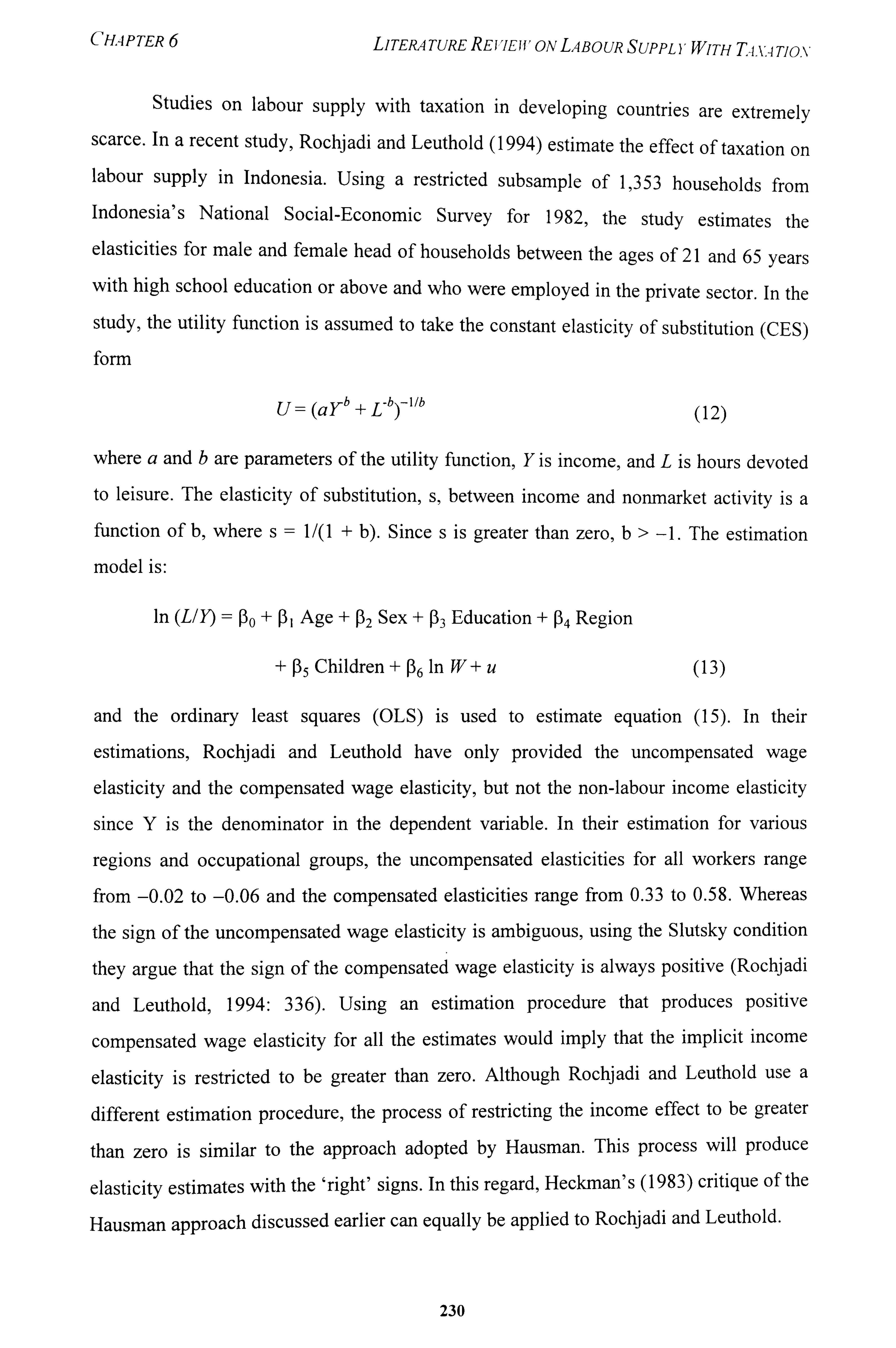
CHAPTER 6 LITERA TURE REVIEWON LABOUR SUPPL YWITH Tix, A TIO-\'

Studies on labour supply with taxation in developing countries are extremely scarce. In a recent study, Rochjadi and Leuthold (1994) estimate the effect of taxation on labour supply in Indonesia. Using a restricted subsample of 1,353 households from Indonesia's National Social-Economic Survey for 1982, the study estimates the elasticities for male and female head of households between the ages of 21 and 65 years with high school education or above and who were employed in the private sector. In the study, the utility function is assumed to take the constant elasticity of substitution (CES) form

U= (aY b+L -b Y Ilb (12)

where a and b are parameters of the utility function, Y is income, and L is hours devoted

to leisure. The elasticity of substitution, s, between income and nonmarket activity is a function of b, where s= 1/(l + b). Since s is greater than zero, b> -1. The estimation

model is:

In (L11) = Po + P, Age +P2Sex +P3Education +P4Region

P5Children +P6 In W+ u (13)

and the ordinary least squares (OLS) is used to estimate equation (15). In their

estimations, Rochjadi and Leuthold have only provided the uncompensated wage

elasticity and the compensated wage elasticity, but not the non-labour income elasticity

since Y is the denominator in the dependent variable. In their estimation for various

regions and occupational groups, the uncompensated elasticities for all workers range

from -0.02 to -0.06 and the compensated elasticities range from 0.33 to 0.58. Whereas

the sign of the uncompensated wage elasticity is ambiguous, using the Slutsky condition

they argue that the sign of the compensated wage elasticity is always positive (Rochjadi

and Leuthold, 1994: 336). Using an estimation procedure that produces positive

compensated wage elasticity for all the estimates would imply that the implicit income

elasticity is restricted to be greater than zero. Although Rochjadi and Leuthold use a

different estimation procedure, the process of restricting the income effect to be greater

than zero is similar to the approach adopted by Hausman. This process will produce

elasticity estimates with the 'right' signs. In this regard, Heckman's (1983) critique of the

Hausman approach discussed earlier can equally be applied to Rochjadi and Leuthold.

230

CHAPTER 6 LITERATURE REVIE[VON LABOUR SUPPLYWITH TAx. 4Tio, v

7. CONCLUSION

From the literature review, it is apparent that issues pertaining to the estimation of labour

supply parameters are complex. Estimation problems abound and challenge the skill and

creativity of analysts for over two decades. After the early estimation efforts in first

generation research, analysts soon realised the importance of paying careful attention to

model specification. This led a new generation of static labour supply research using

advanced techniques. Despite the innovative procedures adopted in second generation

research, the wide range of labour supply parameter estimates persist. Sensitivity

analyses were conducted on the estimation methods, functional forms and assumptions

adopted to determine the source and extent of variation. The results of these studies have

been revealing. Economic and statistical assumptions can have a substantial impact on

the estimates obtained. However, not all of the disparate results are due to differences in

estimation procedure since some studies conduct analysis on subsamples of the same

data set and produce different estimates for each category of the subsample.

The incorporation of taxation in the labour supply model presents additional

problems to the analyst. Under progressive taxation, the budget set is no longer linear but

convex and piecewise linear. The concept of virtual income is used as a device to

linearise the budget set so as to simplify the estimation procedure. An advance to the

estimation methodology was made by Burtless and Hausman (1978) which allowed the

econometric model to have two error terms instead of one, i. e. unobserved heterogeneity

of preferences and optimisation error. The maximum likelihood technique is used to

solve the equations. In the case of the non-convex budget set, Burtless and Hausman

demonstrated the technique of using the Roy's identity to generate the labour supply

function from the indirect utility function. This method is valid as long as the Slutsky

condition holds. Hausman later elaborated on this technique in a number of papers

(Hausman, 1979,1980,1985). While the Hausman approach has been adopted by

analysts in analysing the non-convex budget set as a result of taxes and welfare

programme, Heckman (1983) raises the question whether the Hausman procedure is

trying to 'fine tune' too much in the face of data that neither he nor economists are likely

to have. This is echoed by Mroz (1987: 786) that the Hausman procedure requires

exceptionally strong assumptions on the tax structure and the stochastic disturbances in

231

CHAP TER 6 LITERATURE REFIEIVON LABOUR SUPPLYWITH Tq. v. ATio. \,

the model'. Heckman (1983: 74) argues that 'previous empirical procedures such as those of Boskin and Hall that incorporate less (false) information into the estimation

procedure may be more robust than procedures such as Hausman's which assume information that does not exist and which produce inconsistent estimators if the information is false. ' These arguments provide a case for using the instrumental variable

approach, which has recently been applied on Swedish data.

In the next chapter, we draw from the methodological experience of second

generation work to assess the importance of taxes in the Malaysian labour supply function. We use the instrumental variable approach in the next chapter for this purpose. It is not clear at this stage whether results obtained will correspond to general findings of

studies from developed countries. While there is no a priori reason why this should not

be the case, the differences in the work environment, work culture, and institutional

underpinnings with regards to employment, wages, social security and benefit, and

household income between the developed and developing countries could influence the

final outcome.

232

Chapter 7

MODELLING LABOUR SUPPLY WITH TAXATION

1. INTRODUCTION

After reviewing the relevant literature on static labour supply modelling in the last

chapter, we now proceed to discuss the model specification and the estimation results. This chapter seeks to estimate the labour supply response of married couples in the prime

age groups facing the 1984 and 1992 Malaysian income tax rates. Since 1986 the

marginal rates of the individual income tax have been reduced in stages. The top rate of 55% was reduced to 40% in 1986 and subsequently brought down to 32% in 1995.

The average family income has expanded rapidly relative to tax exemptions and

deductions. As discussed in Chapter 4, the tax base expanded during this period, with

more people now falling within the taxable category as the result of bracket creep. The

reduction of the top marginal tax rate and the growth in average family income resulted

in individuals reaching the top tax bracket faster than they did a decade before. On the

other hand, the marginal tax rate at each taxable income category has fallen. This implies

that households with family income at the national average, or some multiples of it, are

now paying lower taxes. In the light of these developments, it will be interesting and

useful to examine the labour supply response under the tax regimes of 1984 and 1992. In

this chapter, we examine the effect of income tax on the response of individuals towards

participation and hours worked. The purpose of this chapter is to examine the effect of

income tax on work incentives in Malaysia. It will generate elasticities of labour supply

with and without taxation, and the basis of which will provide some indication whether

the treatment of labour supply as an exogenous variable in the tax reform simulations

performed in Chapter 5 is reasonable.

CHAPTER MODELLING LA BO UR SUPPLY WITH T4X, 4 TION

This task of estimating the coefficients of the labour supply function with taxation for Malaysia is very much facilitated by the availability of income and labour force data collected by the Department of Statistics. This estimation will certainly increase our understanding of the labour supply characteristics of countries having

economic, social and institutional structures which differ from the developed countries. While Malaysia may not represent an average developing country in terms of its income

level, growth rate, and rates of unemployment and inflation, it nevertheless shares a similar pattern of development with many high middle income countries, ) especially those in the Far East.

Much of our understanding of labour supply with taxation are derived from

studies conducted in the developed countries which have different tax and transfer

payment structures from the developing countries. For instance, in the developed

countries, taxes on income, profit and capital gains account for 40 per cent of central

government revenue in 1985, while social security contributions account for 30 per cent. The comparable figures for middle income developing countries are 24 per cent and 10

per cent, respectively (World Bank, 1987: Table 24). In Malaysia, total income tax in

1985 contributes about 42 per cent of the federal government revenue and 11.4 per cent

of GDP, while individual income tax constitutes about 20 per cent of the total income tax

collected.

Many of the elaborate welfare and social benefit systems in operation in the

developed countries do not have their equivalent in the developing countries. Without

unemployment benefit and income support programmes, an individual who is out of

work in a developing country will have to fall back on past savings or rely on the

goodwill of relatives. This means that there is a stronger motivation for a person who has

just lost his job to get back to work or perform some part-time work. There is no

financial advantage for him to choose to remain unemployed or to limit his hours of work

as might be the case if he faces a non-convex budget constraint arising from welfare

transfer payments within a progressive tax system. The hours of work put in by members

of a household may also be affected by welfare programmes, or the lack of them.

Without the benefit of income support programmes, poor households in developing

234

CHAPTER 7 MODELLiNG LABOUR SUPPL YWITH T-i, V. 4 TION

countries would have to increase the hours of work to make ends meet. One can argue that under such circumstances some caution should be exercised when trying to make some inferences about the labour supply responses of developing countries on the basis

of studies conducted in developed countries.

Much of the discussion of the backward bending supply curves relates to high

levels of income (Deaton and Muellbauer, 1980; Sapsford and Tzannatos, 1993). An

important assumption in the labour supply model of developed countries is that work is a Giffen good while leisure is a normal good. At higher levels of income, an individual

will demand more leisure and correspondingly, less work. Hence, at higher income

levels, the individual's supply curve of hours becomes backward-sloping as the wage rate

increases because the income effect (which is linked with the demand for more leisure as

income increases) is expected to outweigh the substitution effect (which encourages the

individual to substitute leisure for work as it becomes relatively more expensive).

There is some evidence of backward-bending labour supply curves in developing

countries. These curves occur not at the high income level, but rather among subsistence

farmers in rural communities where income is among the lowest. In his study of the

supply and demand for labour in Rural West Bengal, Bardhan (1984) found that the

supply curve of the hired out farm labourers were backward-bending. Huang (1976)

examines the peasant economy of three paddy areas in Malaysia and argues that

subsistence farmers are not responsive to economic opportunities and behave according

to the notion of a backward-bending supply curve. In examining the effect of taxes on

labour supply in Malaysia, we would also be generating results that could shed some

light whether there is evidence of a backward-bending labour supply curve for the whole

economy, and not just among subsistence farmers, and if so, at what income level is it

most evident.

The remainder of this chapter is organised as follows: Section 2 discusses the

sources of data and concepts on labour force and household income used in the analyses.

This is followed by a discussion on the labour force and income characteristics in Section

3. The model specifications on estimating the labour supply coefficients before and after

235

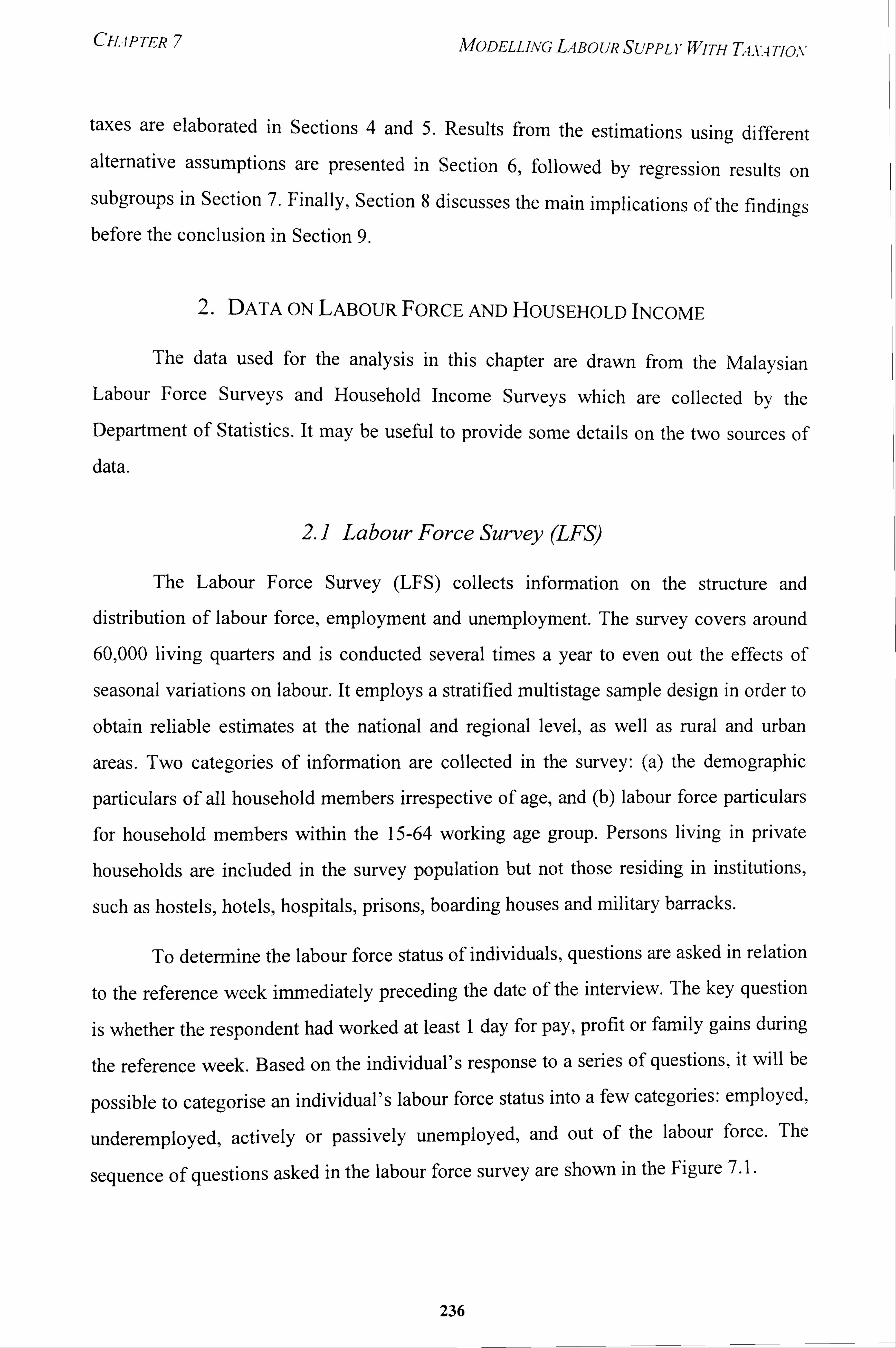
CILIPTER 7 MODELLjNG LABOUR SUPPLYWITH TAx, 4 Tiox

taxes are elaborated in Sections 4 and 5. Results from the estimations using different

alternative assumptions are presented in Section 6, followed by regression results on subgroups in Section 7. Finally, Section 8 discusses the main implications of the findings before the conclusion in Section 9.

2. DATA ON LABOUR FORCE AND HOUSEHOLD INCOME

The data used for the analysis in this chapter are drawn from the Malaysian

Labour Force Surveys and Household Income Surveys which are collected by the Department of Statistics. It may be useful to provide some details on the two sources of data.

2.1 Labour Force Survey (LFS)

The Labour Force Survey (LFS) collects information on the structure and distribution of labour force, employment and unemployment. The survey covers around

60,000 living quarters and is conducted several times a year to even out the effects of

seasonal variations on labour. It employs a stratified multistage sample design in order to

obtain reliable estimates at the national and regional level, as well as rural and urban

areas. Two categories of information are collected in the survey: (a) the demographic

particulars of all household members irrespective of age, and (b) labour force particulars

for household members within the 15-64 working age group. Persons living in private

households are included in the survey population but not those residing in institutions,

such as hostels, hotels, hospitals, prisons, boarding houses and military barracks.

To determine the labour force status of individuals, questions are asked in relation

to the reference week immediately preceding the date of the interview. The key question

is whether the respondent had worked at least I day for pay, profit or family gains during

the reference week. Based on the individual's response to a series of questions, it will be

possible to categorise an individual's labour force status into a few categories: employed,

underemployed, actively or passively unemployed, and out of the labour force. The

sequence of questions asked in the labour force survey are shown in the Figure 7.1.

236

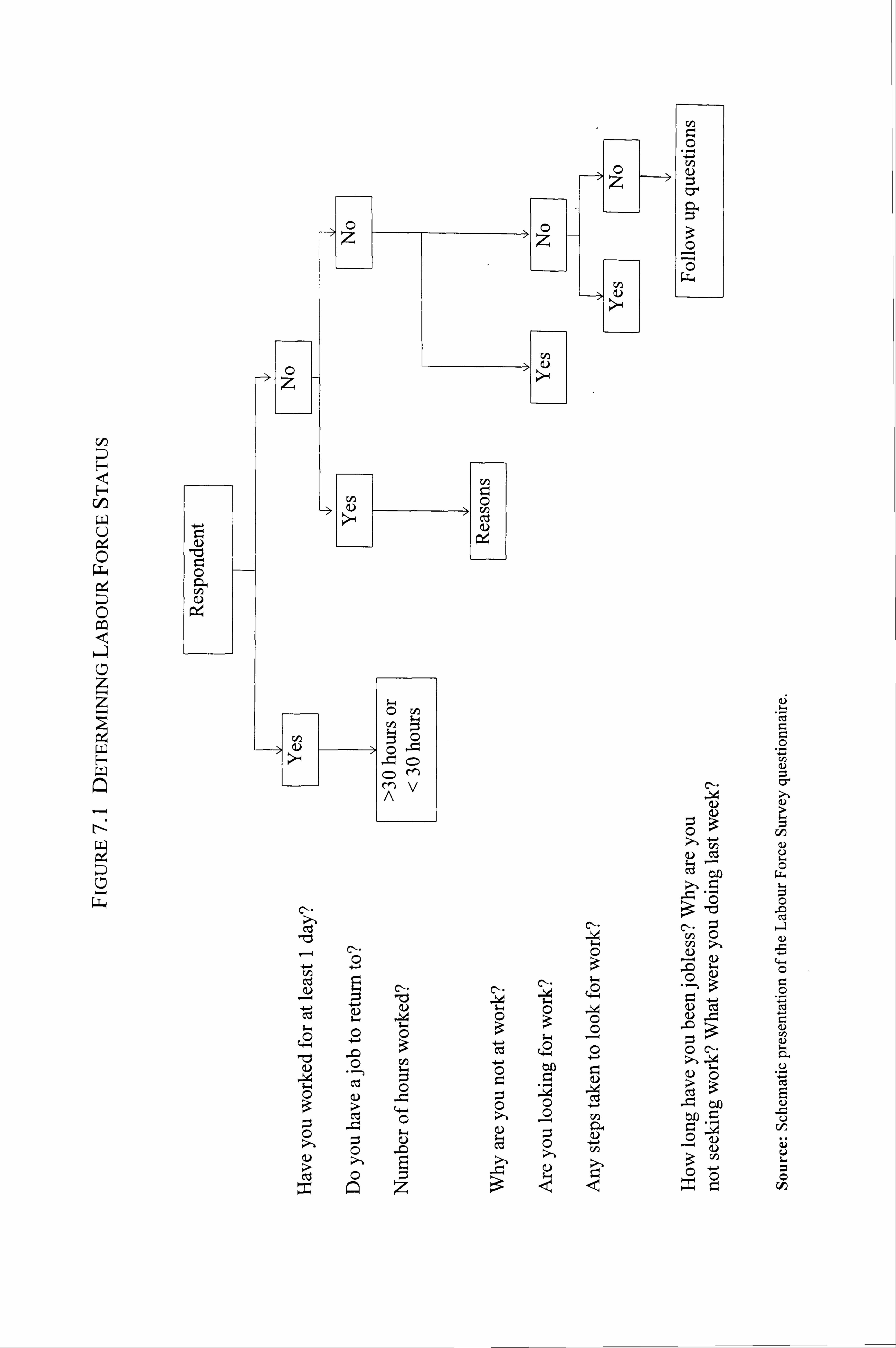
(ID H

H ccJ LU U

C

0

Cý-

03

CA

Cd Cl. C-.

7ý

0

ct

Cl.

7ý

C-.

0 0

ct

+. 4

CI--

-0 ; -4

CD

u

C)

Z.,

cn

zi 0

-0

CHAPTER 7 MODELLiNG LABOUR SUPPL YWITH T-i. u Tim,

2.1.1 Determining labour force status

A person's labour force status is determined on the basis of his or her responses to the questions asked in the LFS. If a person answers 'Yes' to Question 1, the he/she

will be asked Question 3 to determine the number of hours worked. If the answer is 'No'

to Question 1, then he/she will be asked Question 2 of whether he/she has a job to return to. If the answer is 'Yes' to Question 2, then he/she is asked why he/she was not at work during the reference week. If the answer is 'No' to Question 2, Questions 5-7 are asked to determine the nature of unemployment.

Response of 'Yes' to Question I

1. If a respondent has worked for at least I day in the reference week, he or she is

considered 'employed'.

2. If a respondent worked less than 30 hours, he or she is 'underemployed'.

Response of 'No' to Question I

1. If a respondent is not working but has job to return to, he or she is 'employed'.

2. If a respondent is not working but looking for work, he or she is 'unemployed'.

3. If a respondent is not working and not looking for work, he or she is asked the reasons

for not looking for work. If the respondent believes that there is no job available, or

because of bad weather, illness, confinement, waiting for answer from an application,

and no qualifications, then he or she is regarded to be 'passively unemployed'. If the

respondent is schooling, a housewife, disabled, retired, or not interested in working, then

he or she is considered to be 'out of the labour force'. Except for those out of the labour

force, all others in the 15-64 age groups are considered to be part of the labour force.

2.2 Household Income Survey (HIS)

There are few household income surveys in the past. Income data at the beginning

of the seventies can be obtained from the Post Enumeration Survey (PES) of the

Population Census 1970. While conducting PES to ascertain the extent of census

238

CH. -IPTER 7 MODELLiNG LABOUR SUPPL YWITH T4X4 TION

undercounting, the Department of Statistics included questions on household income in

the survey. In the mid-seventies, the Agricultural Census 1976 contains some questions

on household income. After the Agricultural Census, there was a long lapse before the Household Income Survey (HIS), specifically designed to collect household income data,

was conducted in 1984. Starting from this survey, the Department of Statistics adopts the

strategy of conducting HIS at regular intervals. The Household Income Surveys are

attached to the Labour Force Surveys so that the two surveys can be conducted

simultaneously for the same sample of households. The HIS for 1984,1987,1989, and 1992 were conducted using this strategy. After gathering information on household and

labour force characteristics using the Labour Force Survey questionnaire, the

interviewers then proceed to obtain income data from the same individuals. Since the

households and individuals for the two surveys are similar, it is possible to combine the

information from the two surveys to yield a complete record which contains information

on household, labour force and income characteristics of an individual.

The HIS collects data on income, taxes as well as transfer receipts and payments

for the whole year, using the previous year as the reference year. Where information

cannot be obtained directly, interviewers use work sheets to calculate the imputed value

of agricultural and non-agricultural activities, home produce consumption, as well as rent

for dwelling and agricultural land.

2.3 Concept ofHousehold Income

2.3.1 Earnings

There are two categories of earnings: paid employment income and self

employment income (see Table 7.1). Paid employment income includes wages and

salaries, allowances,, bonuses, commissions and tips, overtime earnings, free food,

free/concessional lodging and consumer goods, other payment in kind, and employers

contribution to the Employees Provident Fund. If a person is not an employee but is self

employed, his or her income is classified as income accrued from self employment.

239

CHAPTER MODELLiNG LABOUR SUPPL YWITH T4-VA TION

TABLE 7.1 ANNUAL HOUSEHOLD INCOME DURING THE LAST 12 MONTHS

EARNINGS

1. Earnings during the last twelve months from paid employment i. Wages and salaries (before income tax, social security contributions, etc. )

ii. Allowances (e. g. cost of living allowances, specialist allowances, housing allowances) iii. Bonuses iv. Other cash (like commissions, tips, earnings from overtime work, etc. ) V. Free concessional food v i. Free concessional lodging

vii. Free concessional consumer goods and services viii. Other payments received in kind (like paddy, coconut, rubber, etc. )

ix. Employer's contributions to social security A. Total Paid Employment Income

2. Earnings from self employment during the last twelve months 3. Receipt during the last month from

i. Imputed rent of owner-occupied house ii. Rent from houses or other property iii. Rent from lodging

B. Total Other Earned Income

INCOME OTHER THAN EARNINGS

4. Income received during the last twelve months from property i. Royalties (in respect of copyrights, patents and similar rights)

ii. Rent from agricultural land iii. Interest (from banks, deposits, bills, bonds, loans, etc. ) iv. Dividends (such as from ownership of shares)

C. Total Property Income

5. Income received during the last twelve months from transfers i. Remittances (from other households from within and outside the country)

ii. Alimony iii. Scholarships / Bursaries / Fellowships iv. Pensions v. Other periodic payments received (e. g. from an inheritance or trust fund, etc. )

vi. Gifts in cash and in kind D. Total Current Transfers Received

TOTAL INCOME [A +B+C+ DI

Source: Surnmarised from the Household Income Survey questionnaire

240

CHAPTER 7 MODELLjNG LABOUR SUPPLYWITH TAX4 TIOA

2.3.2 Income other than earnings

This category of income consists of property income and transfer income. Royalties, rent from agricultural land, interest, and dividends are considered property income, while transfer income, scholarships, pensions, and gifts received are classified as current transfer income. The summation of earnings and income other than earnings

constitutes the total income of an individual in a household.

2.4 Sample Usedfor Analysis

The analysis uses a 25 per cent sample of households from the combined data of

the Labour Force Survey and the Household Income Survey for 1984 and 1992. The

subsample is randomly selected from the survey tape on the basis of households so that

the individual records for the selected households appear together. There are about 60,000 individual records on both adults and children for each of the two years. Care is

taken to ensure that the households included in the subsample are identical for both LFS

and HIS. After verifying that the household indentifiers of the two data sources match

exactly, the two data sources are merged. The analysis on households is only confined to

the year of the survey. No attempt has been made to combine the data across several

years for a longitudinal analysis since a different sample of households is selected for

each of the years.

The focus of the study is to examine the participation and labour supply of males

and females within the household context. The data base consists of the head of

household and his or her spouse who are in the prime age group of 20-54 years. The joint

income and joint taxes of the couple are calculated and attached to the couple's record

together with the number and ages of their children. Included in the sample are

employees, own account workers, housewives, and those of other employment status, but

not employers and students. The inclusion of employers would complicate the

relationship between earnings and hours of work since only part of their earnings can be

attributed to their own labour input. Students are excluded because they are technically

out of the labour force. Housewives are included in the sample because most married

women who are not working would be classified into this category. Since we wish to

241

CHAPTER 7 MODELLiNG LABOUR SUPPLYWITH T4. vA Tjo. v

consider the participation decision of married women, it is necessary to include housewives in the data.

2.5 Concepts Used in the Model

Participation: This variable refers to those who supply positive hours of work during the reference week and non-participation to those who work zero hours. Those

who are out of the labour force are not considered in the participation formulation. ' Prior

to the late 1960s analysts failed to distinguish between participation (employment) and hours of work. This distinction is important because labour supply coefficient estimates based on participation show greater responsiveness to wage and income variation than hours-of-work equation. Heckman (1993) notes that labour supply empirical studies in

1960s showed that the wage and income elasticities are higher for females than for male largely because analysts were using elasticity estimates from the participation equation for females and elasticity estimates from the hours-of-work equation for men. Mroz

(1987) dismissed the conventional wisdom that the wage and income elasticities for

women are larger than men when he controlled for self-selection bias in the participation

equation. This finding concurs with Nakamura and Nakamura (198 1) and is supported by

Thomas MaCurdy, Green and Paarsch (1990). 2

TT-

hours: This variable refers to hours of work per week. Hours are positive for

those who are working, and zero for those not working. The measurement of hours is a

potential source of error because there is inadequate data for paid holidays, absenteeism,

time not working due to illness, overtime etc. In addition, the number of hours worked

during the reference week need not be the typical hours worked throughout the year.

Should an individual work overtime during the reference week, there will be errors in

calculating the number of hours worked and, correspondingly, the average wage, which

uses hours worked as the denominator. Another source of error is that the observed hours

I There is a difference in the usage of the term 'participation' in the labour supply literature and the

Labour Force Survey. In labour supply analysis, participation refers to positive hours of work and non-

participation to zero hours of work. In the Labour Force Survey, labour force participation refers to

those in the 15-64 age group who are not 'out of the labour force'.

More discussion on this issue is found in Chapter 6.

242

CHAPTER 7 MODELLING LABOUR SUPPLYWITH T-i-v-i Tiov

do not correspond to the desired hours because of constraints on the supply side (e. g. health) or the demand side (such as minimum or maximum hours and institutional working hours). In the sample, we have removed those who are employed but reported zero hours of work in the reference week, as a result of being on a holiday, illness, strike, etc. Their inclusion would complicate the calculations since they would appear to be

earning wages for supplying zero hours of work.

Wage: The Labour Force Survey does not collect wage data. To derive this

variable, annual labour earnings is divided by the hours of work per year, i. e. hours

worked during the reference week multiplied by 52 to yield the wage rate before tax (w). The net wage rate or marginal wage (WAGETAX) is given by w(l - T)where w is the

wage rate and T is the marginal tax rate. The marginal tax rate is calculated from the income tax paid by the individual as reported in HIS. Based on the amount of taxes paid

reported, it is possible to derive an individual's marginal tax rate, that is, his or her tax bracket. The marginal wage is used to find the point of tangency between the utility function and the budget constraint in order to determine the hours of work. Theoretically,

it is the marginal wage rather than the average wage that an individual is concerned with in deciding whether to put in an extra hour of work. In many studies, the marginal wage

is estimated from official income tax schedules calculated on the basis of reported income. In this case, assumptions need to be made about the amount of allowable

deductions and the extent of separate or joint assessment of the income of married

couples. The calculated tax is unlikely to correspond with the actual amount of tax paid

by the individual since it overlooks tax avoidance and evasion. Since hours of work is

used to derive WAGETAX, errors in measuring hours are transmitted to the

measurement of wage.

Non-Labour Income Variable: This variable is equal to an individual's total

income minus his/her labour income plus the total income of his or her spouse. There is

the practical problem of estimating the non-labour portion of an individual's income. In

some cases, it may require imputing the value of the rental of owner-occupied dwellings

and goods produced for own consumption. The model considers only income from the

spouse and not the other people in the household. Some older couples may have married

243

CH. 4PTER 7 MODELLING LABOUR SUPPL YWITH T, 4. v, -i Tim'

children or other relatives living in the same household but it is difficult to say to what extent their income affect the labour supply of the couple. In most Asian families, the

men are the main breadwinner, as indicated by over 95 per cent of married men who were reported as being the head of household.

Education (EDUQ: Dummy variables are used for primary, lower secondary,

upper secondary, and tertiary education against the reference group of those not having

any education. The US provides the highest level of educational attainment for each household member.

Experience (EXPRQ: This variable refers to potential work experience, which is

measured in years and is used only for males. This variable is estimated because LFS

does not collect information on work experience. To calculate this variable, we estimate

the age of leaving school, i. e. years of schooling plus 6, which is the first age of

schooling. If the age of leaving school is greater than 15 years, then the potential work

experience variable of an individual is his age minus the age of leaving school. If the age

of leaving school is less than 15 years, then the potential work experience variable is

assumed to be an individual's age minus 15. The rationale for using 15 years as a cut off

point is because there is automatic promotion up to 9 years of schooling, while child

labour is a non-issue in Malaysia. It may be argued that children below 15 years may

help out in the farm or family business and that would contribute to their experience. The

model, nevertheless, assumes that an individual would begin to accumulate work

experience that would make a difference to his wage only after 15 years of age. The work

experience variable can be used for the males without much problem because of their

high participation rate and very low unemployment rate, which means that there is no

breaks in estimating an individual's work experience. This variable is not used for

females since there may be career breaks in a woman's life-cycle and on which we have

no information.

Children: Dummy variables are used for children in different age groups, i. e. I

year and less (CHI), 2 years (CH2), three to five years (CH3_5), six to eleven years

(CH6_1 1), and twelve to sixteen years (CH12_16). In LFS, age is reported in years. The

244

CHAPTER 7 MODELLiNG LABOUR SUPPLYWiTH T4,, v. 4 Tiox

age group 6-11 years corresponds with 6 years of primary education, while the age group 12-16 years corresponds with 5 years of secondary education. Children undergoing tertiary education and high school are above 16 years old where many would have to leave home to attend college or university.

Urban (URB) is a dummy for all gazetted areas with population of 10,000 and above. This variable refers to the place of dwelling and is not necessarily the work place of a respondent.

Occupation: The classification of occupation follows the Malaysian Dictionary of Occupational Classification which adopts the recommendations of the International

Labor Organization. The acronyms for the occupations used in the model are as follows:

TEACH = teachers who are classified under the professional and technical

occupation. Teachers generally report lower hours of work, averaging 25-30

hours per week. In collecting this information, it is clear that US takes into

account the time spent during normal schooling hours but not the time spent by

teachers on extra-mural activities, preparation of teaching materials, and marking

of school work outside schooling hours.

PROF = professional and technical workers, excluding teachers; ADM =

administrative and managerial workers; CLR = clerical workers; SALE = sales

workers; SER = service workers; AGRIWKR = agricultural workers, who are not

necessarily farmers since this occupational group include estate managers,

planters, and fishermen as well; and PROD = production workers.

3. LABOUR FORCE AND INCOME CHARACTERISTICS

Malaysia's labour force was growing at an annual growth rate of 2.7 per cent and is

estimated to be 8.1 million in 1995. During the last 10 years, the size of the labour force

was growing at 2.9 per cent per annum, while the labour force participation rate for those

in the 15-64 age group was 67 per cent. Although the unemployment rate peaked at 8.8

per cent in 1986 during the height of the recession, it has fallen steadily to around 3.0 per

cent for the last three years when the country reached full employment of its workforce.

245

CHAPTER 7 MODELLING L. 4BOUR SUPPLYWJTH T-i, v. 4 Tio, v

According to Lucas and Verry (1990), married women plays an important role in bringing about labour force adjustments as economic conditions change, both cyclically and in the long term. Despite the recent increases in labour force participation of females, their participation rates for all age groups are below 50 per cent and married women tend to respond readily to economic incentives, such as changes in wages, labour market conditions, educational opportunities, etc.

The effects of education on labour force participation in Malaysia do not form a

clear pattern. Except for those with primary education, individuals of either sex are more likely to participate in the workforce as their educational levels increase. This pattern is

more marked for females than for males. Those with primary education have higher

participation rates than those with lower secondary education (Lucas and Verry, 1990: 5).

Participation seems to be higher in rural than in urban areas, although the nature of

participation in the two strata may not share similar characteristics. For instance, women in rural areas may perform agricultural activities alongside their other household

activities.

Household income grew rapidly during the last two decades. This was

accompanied by the reduction of the poverty incidence of 49.3 per cent in 1970 to 16.7

per cent in 1990 (Malaysia, 1991a: 43). Households benefited from productivity

increases and structural changes in rural employment that widen the scope of economic

activities and raised income. The expansion in non-agricultural jobs encouraged large

numbers of self-employed and unpaid family workers to enter the waged labour market

and made wage income an important component of income in rural areas.

Table 7.2 shows the mean and standard deviation of the variables for males and

females in the sample based on the combined Labour Force Survey and Household

Income Survey (LFS/HIS) data set for 1984 and 1992. The sample consists of married

heads of household and his/her spouse in the prime age groups. The average age in the

sample is 38 years for males and 36 years for females, both of whom have around 6-7

years of education. Waged employment is the most important source of income for the

average individual, while the income accrued from self-employment is much smaller.

246

CHAPTER 7 MODELLiNG LABOUR SUPPLYWiTH TIV4 TION

The contribution of property income and net transfer income to the total income of an average male is small, although the contribution of net transfer income to female income is slightly larger than the males. Average income has increased between 1984-1992 and average hours worked have risen by 2 hours for males and I hour for females.

In terms of hours worked, four-fifths of the males in urban areas and three- quarters in the rural areas work between 31-60 hours per week (see Table 7.3). Among females, two-thirds of the workers in the urban areas and three-fifths of workers in the rural areas work between 31-60 hours per week. The degree of under employment, i. e. people working below 30 hours per week, is larger in rural areas than urban areas and for females than males. This corresponds with the nature of agricultural activities in rural areas, which are influenced by weather and outdoor working conditions, seasonality and minimal manpower input required during the growth phase of some field crops. Women

who work shorter hours per week are normally involved in part-time work to augment family income while performing their household activities. The degree of

underemployment was generally lower in 1992 than 1984.

The distributions of taxes paid and marginal tax rates are shown in Table 7.4 and Table 7.5, respectively. The majority of people in the labour force in Malaysia do not pay income tax. An important reason for this is the low net wage earned by the average

worker (see Table 7.2). About three-quarters of the males are non-taxpayers and among

those who pay taxes, the median taxpayer falls within the 12 per cent tax bracket. The

proportion of females who are non-taxpayers is even larger than the males, attributable to

the lower female participation rate (38 per cent in 1984 and 40 per cent in 1992) as

against 97 per cent for the males. Over 90 per cent of females do not pay taxes although

the percentage of female non- taxpayers is lower in 1992 than it was six years before.

The median female taxpayer has also moved up the tax bracket, from 9 per cent in 1984

to 12 per cent in 1992.

247

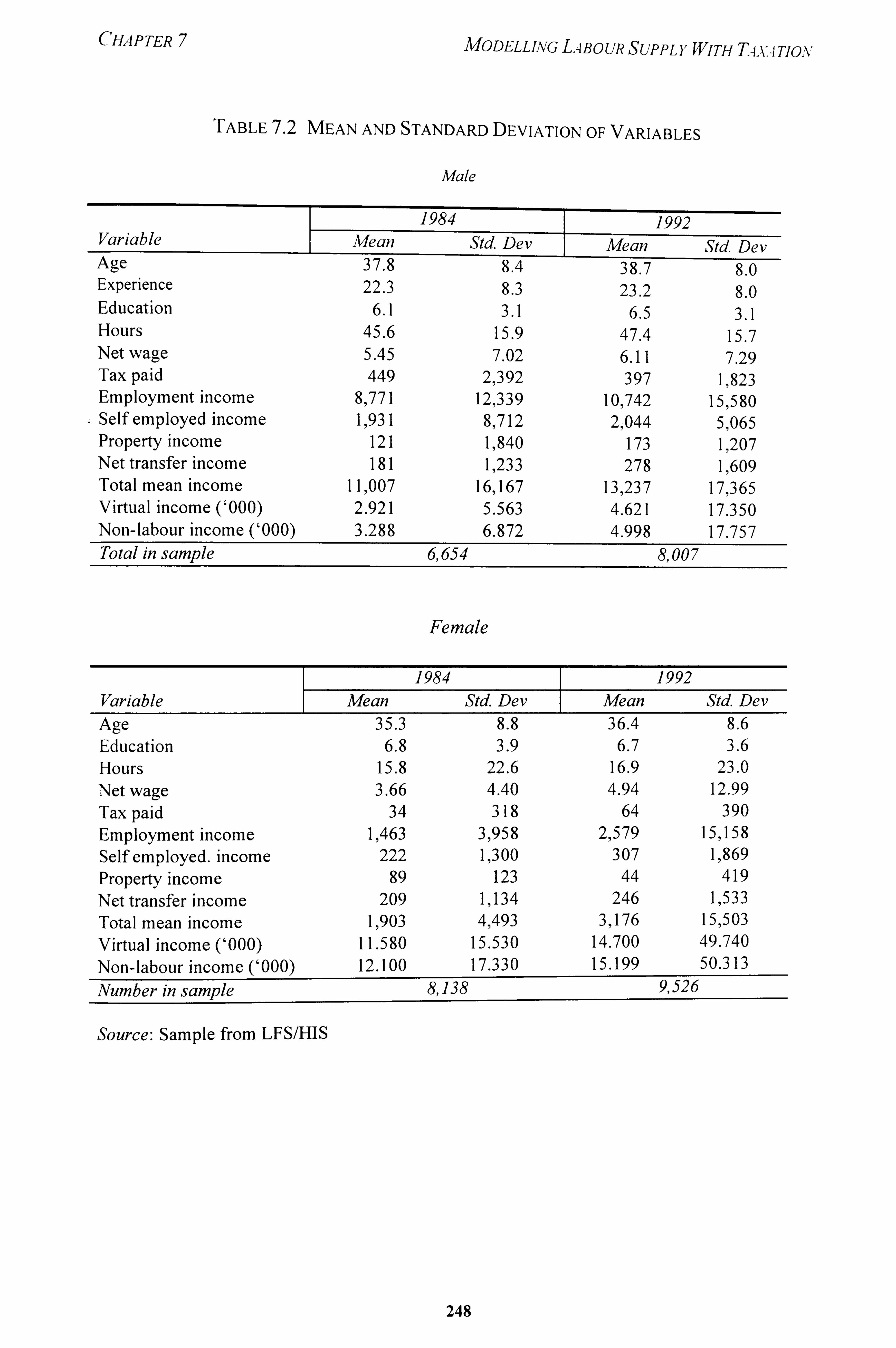
CHAPTER 7 MODELLiNG LABOUR SUPPLYWiTH T-LV. 4 Tlo,, \,,

TABLE 7.2 MEAN AND STANDARD DEVIATION OF VARIABLES

Male

1984 1992 Variable Mean Std DeV Mean Std Dev Age 37.8 8.4 38.7 8.0 Experience 22.3 8.3 23.2 8.0 Education 6.1 3.1 6.5 3.1 Hours 45.6 15.9 47.4 15.7 Net wage 5.45 7.02 6.11 7.29 Tax paid 449 21392 397 1,823 Employment income 8,771 12,339 10,742 15,580 Self employed income 11931 81712 2,044 5,065 Property income 121 11840 173 1,207 Net transfer income 181 11233 278 1,609 Total mean income 11 ý007 165167 13,237 17,365 Virtual income ('000) 2.921 5.563 4.621 17.350 Non-labour income ('000) 3.288 6.872 4.998 17.757 Total in sample 6,654 8,007

Female

1984 1992 Variable Mean Std. Dev Mean Std. Dev Age 35.3 8.8 36.4 8.6 Education 6.8 3.9 6.7 3.6 Hours 15.8 22.6 16.9 23.0 Net wage 3.66 4.40 4.94 12.99 Tax paid 34 318 64 390 Employment income 19463 31958 29579 15,158 Self employed. income 222 1,300 307 11869 Property income 89 123 44 419 Net transfer income 209 1,134 246 1,533 Total mean income 15903 4,493 3!, 176 15ý503 Virtual income ('000) 11.580 15.530 14.700 49.740 Non-labour income ('000) 12.100 17.330 15.199 50.313 Number in sample 8,138 9,526

Source: Sample from LFS/HIS

248

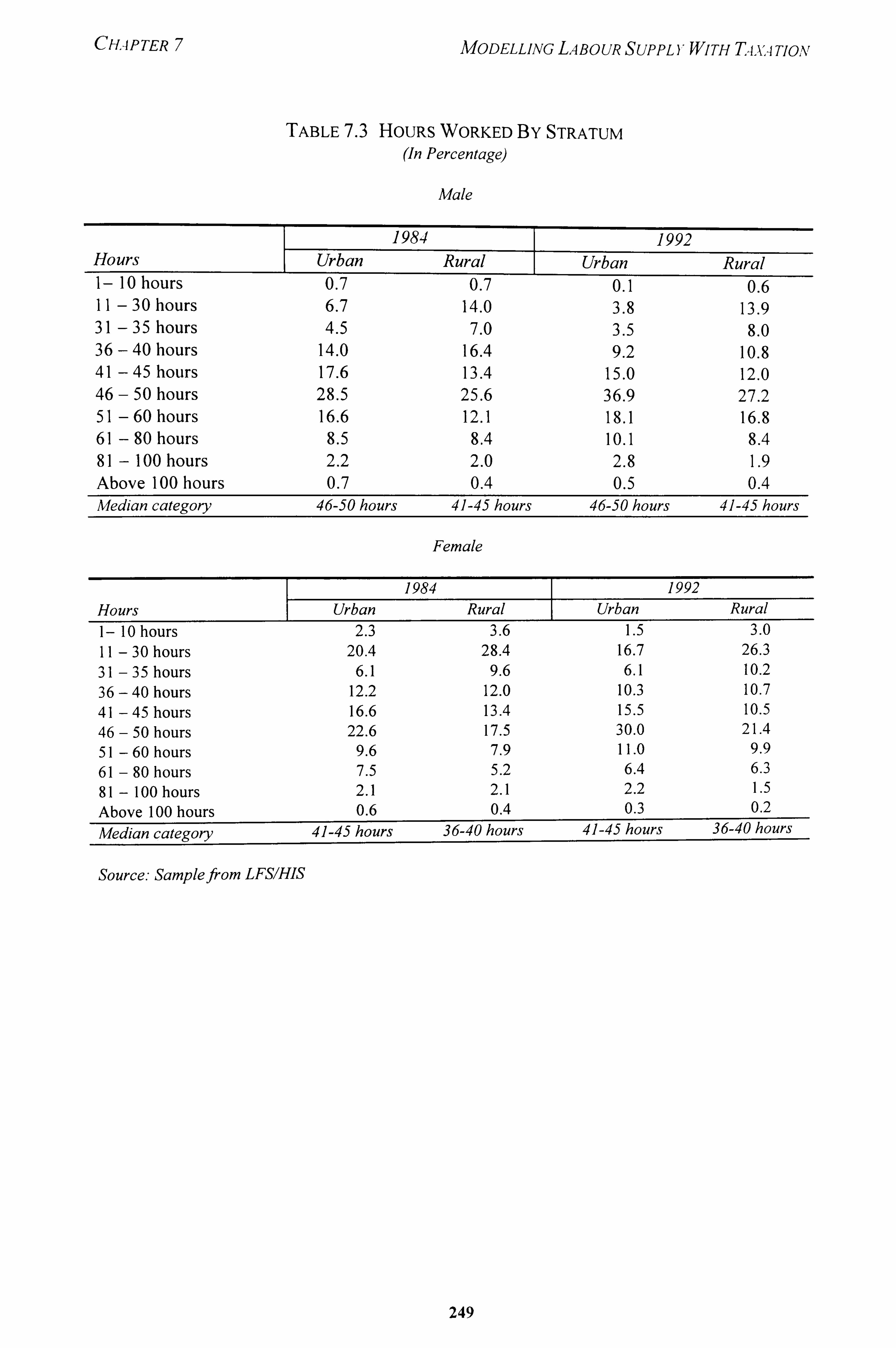
CHAPTER 7 MODELLING L. 4 BO UR SUPPLY WITH T4, v, 4 TioN

TABLE 7.3 HOURS WORKED By STRATUM (In Percentage)

Male

1984 1992 Hours Urban Rural Urban Rural I- 10 hours 0.7 0.7 0.1 0.6 11 - 30 hours 6.7 14.0 3.8 13.9 31 - 35 hours 4.5 7.0 3.5 8.0 36 - 40 hours 14.0 16.4 9.2 10.8 41 - 45 hours 17.6 13.4 15.0 12.0 46 - 50 hours 28.5 25.6 36.9 27.2 51 - 60 hours 16.6 12.1 18.1 16.8 61 - 80 hours 8.5 8.4 10.1 8.4 81 - 100 hours 2.2 2.0 2.8 1.9 Above 100 hours 0.7 0.4 0.5 0.4 Median category 46-50 hours 41-45 hours 46-50 hours 41-45 hours

Female

1984 1992 Hours Urban Rural Urban Rural I- 10 hours 2.3 3.6 1.5 3.0 11 - 30 hours 20.4 28.4 16.7 26.3 31 - 35 hours 6.1 9.6 6.1 10.2 36 - 40 hours 12.2 12.0 10.3 10.7 41 - 45 hours 16.6 13.4 15.5 10.5 46 - 50 hours 22.6 17.5 30.0 21.4 51 - 60 hours 9.6 7.9 11.0 9.9 61 - 80 hours 7.5 5.2 6.4 6.3 81 - 100 hours 2.1 2.1 2.2 1.5 Above 100 hours 0.6 0.4 0.3 0.2

Median category 41-45 hours 36-40 hours 41-45 hours 36-40 hours

Source: Sampleftom LFSIHIS

249

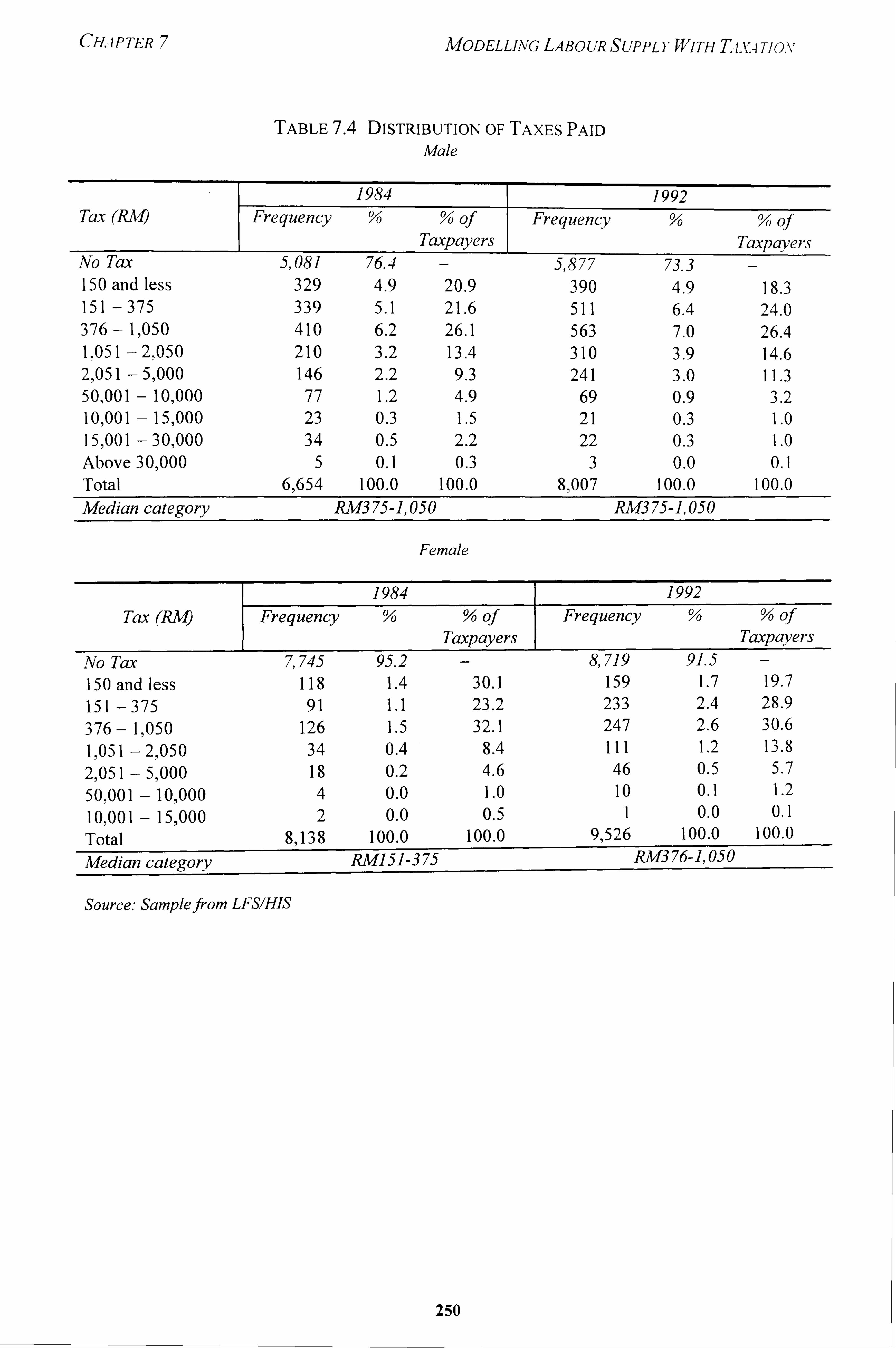
CHAPTER 7 MODELLING LABOUR SUPPLYWITH T4. v4 TIOY

TABLE 7.4 DISTRIBUTION OF TAXES PAID Male

1984 1992 Ta x (R M) Frequency % % of Frequency % % of

Taxpayers Taxpayers No Tax 5,081 76.4 - 5,877 73.3 150 and less 329 4.9 20.9 390 4.9 18.3 151 -375 339 5.1 21.6 511 6.4 24.0 376- 1,050 410 6.2 26.1 563 7.0 26.4 1,051 - 2,050 210 3.2 13.4 310 3.9 14.6 2ý051 - 5,000 146 2.2 9.3 241 3.0 11.3 50,001 - 10,000 77 1.2 4.9 69 0.9 3.2 10,001 - 15,000 23 0.3 1.5 21 0.3 1.0 155001 - 301,000 34 0.5 2.2 22 0.3 1.0 Above 30,000 5 0.1 0.3 3 0.0 0.1 Total 65654 100.0 100.0 8,007 100.0 100.0 Median category RM375-1,050 RM375-1,050

Female

1984 1992 Tax Frequency % % of Frequency % % of

Taxpayers Taxpayers No Tax 7,745 95.2 8,719 91.5 - 150 and less 118 1.4 30.1 159 1.7 19.7 151 -375 91 1.1 23.2 233 2.4 28.9 376- 11050 126 1.5 32.1 247 2.6 30.6 1,051 - 29050 34 0.4 8.4 111 1.2 13.8 2,051 - 5ý000 18 0.2 4.6 46 0.5 5.7 50,001 - 10,000 4 0.0 1.0 10 0.1 1.2 10,001 - 15,000 2 0.0 0.5 1 0.0 0.1

Total 8,138 100.0 100.0 91526 100.0 100.0

Median category RM151-375 RM376-1,050


250

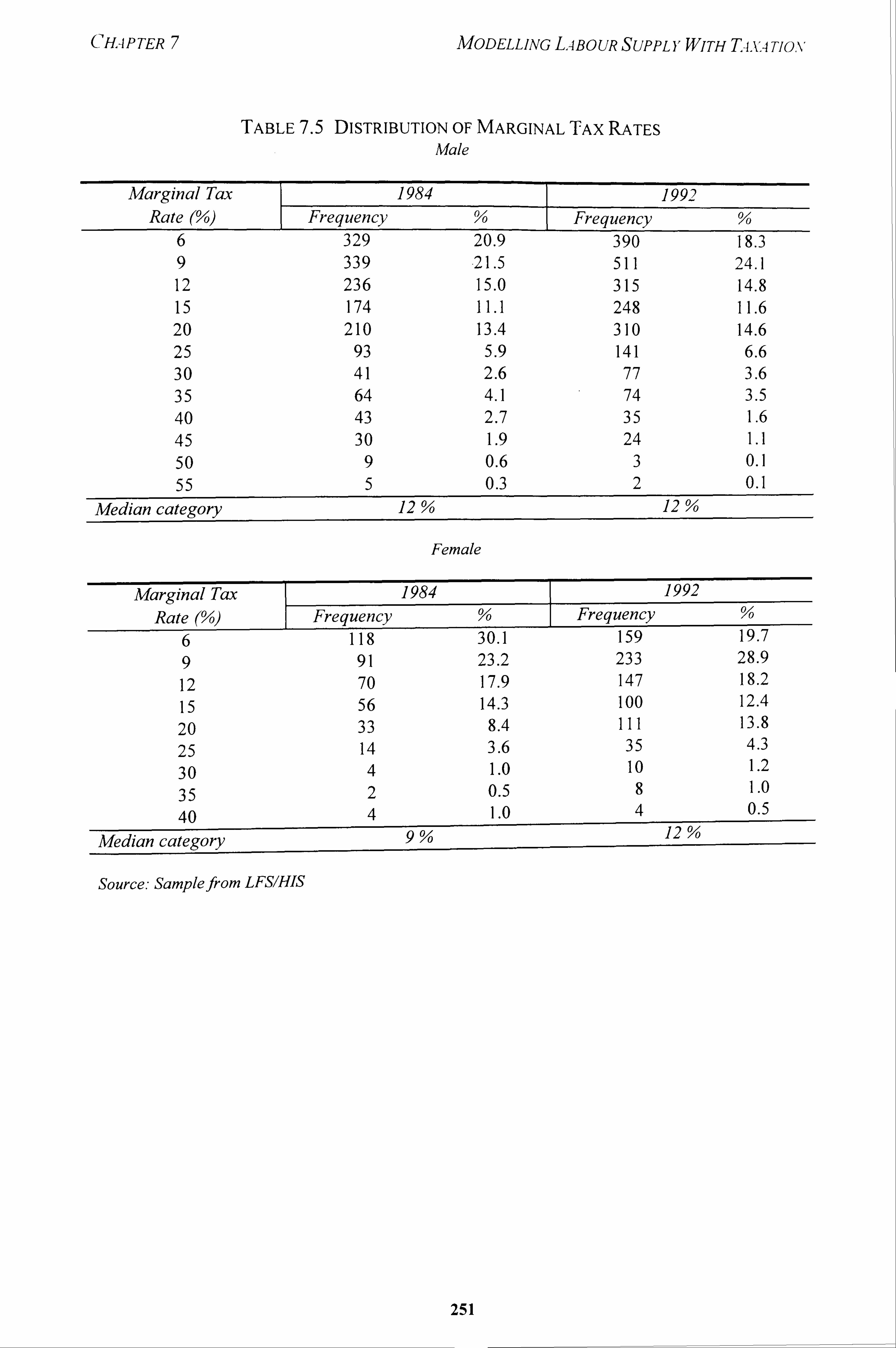
CH, qPTER 7 MODELLING LABOUR SUPPLYWITH TA. v, 4 Tlo, %,

TABLE 7.5 DISTRIBUTION OF MARGINAL TAX RATES Male

Marginal Tax Rate (1/o)

6 9 12 15 20 25 30 35 40 45 50 55

1984 Frequency % Frequency

329 20.9 390 339 21.5 511 236 15.0 315 174 11.1 248 210 13.4 310

93 5.9 141 41 2.6 77 64 4.1 74 43 2.7 35 30 1.9 24

9 0.6 3 5 0.3 2

18.3 24.1 14.8 11.6 14.6 6.6 3.6 3.5 1.6 1.1 0.1 0.1

Median category 12% 12%

Female

Marginal Tax 1984 1992 Rate ('16) Frequency % Frequency %

_ 6 _ 118 30.1 159 19.7 9 91 23.2 233 28.9 12 70 17.9 147 18.2

15 56 14.3 100 12.4

20 33 8.4 111 13.8

25 14 3.6 35 4.3

30 4 1.0 10 1.2

35 2 0.5 8 1.0

40 4 1.0 4 0.5

Median category 9% _12

%


251

1992

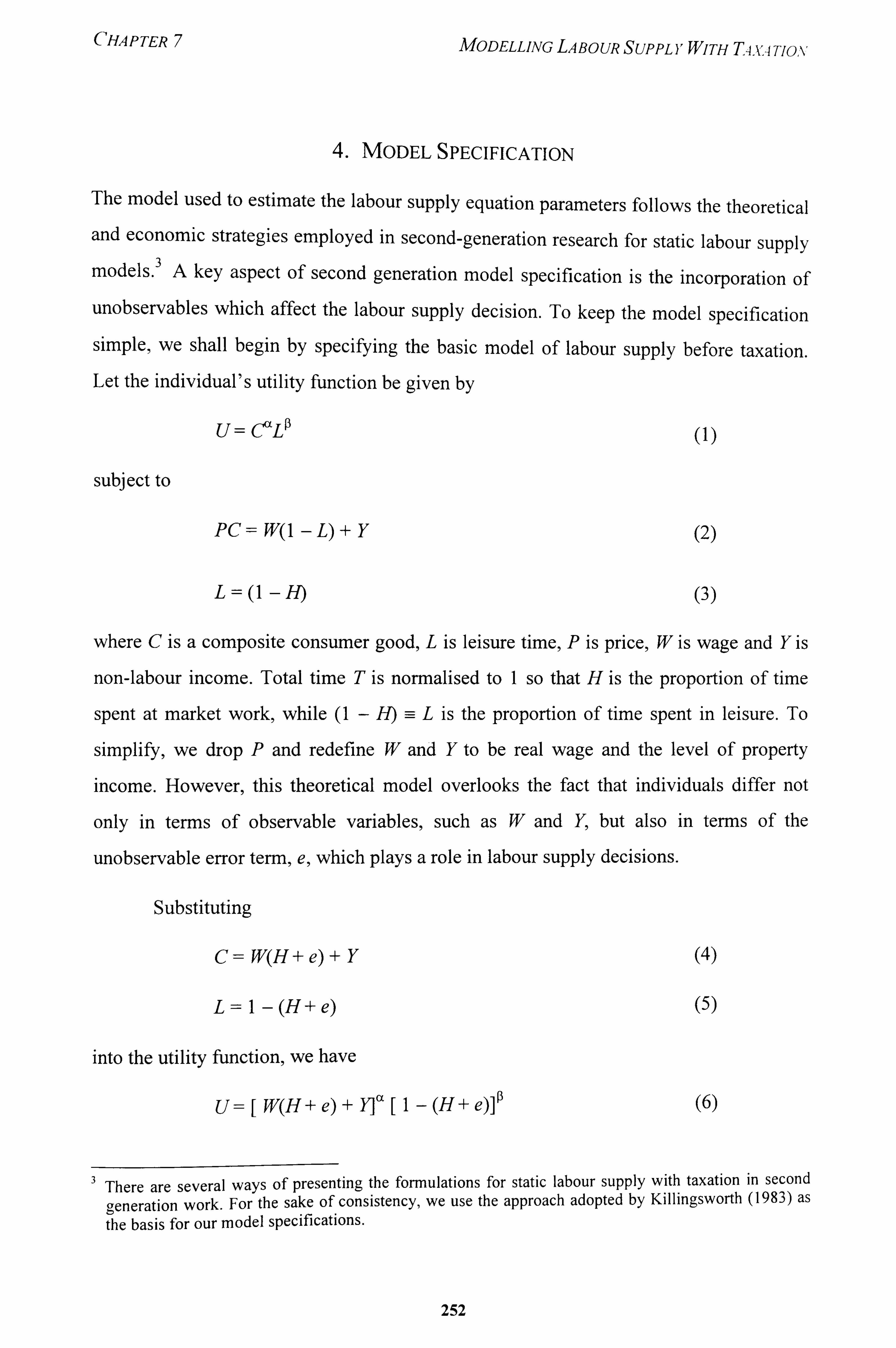
CHAPTER 7 MODELLiNG LABOUR SUPPLYWITH Ta, -i Tiox

4. MODEL SPECIFICATION

The model used to estimate the labour supply equation parameters follows the theoretical

and economic strategies employed in second-generation research for static labour supply models. 3A key aspect of second generation model specification is the incorporation of unobservables which affect the labour supply decision. To keep the model specification simple, we shall begin by specifying the basic model of labour supply before taxation. Let the individual's utility function be given by

U= COV (1)

subject to

PC= W(I -L)+ Y

L=(l -H)

where C is a composite consumer good, L is leisure time, P is price, W is wage and Y is

non-labour income. Total time T is normalised to I so that H is the proportion of time

spent at market work, while (I - H) -= L is the proportion of time spent in leisure. To

simplify, we drop P and redefine W and Y to be real wage and the level of property

income. However, this theoretical model overlooks the fact that individuals differ not

only in terms of observable variables, such as W and Y, but also in terms of the

unobservable error term,, e, which plays a role in labour supply decisions.

Substituting

C= W(H+e)+ Y

L= I -(H+e)

into the utility function, we have

W(H+ e) + ll'x [I- (H+ e)f (6)

3 There are several ways of presenting the formulations for static labour supply with taxation in second

generation work. For the sake of consistency, we use the approach adopted by Killingsworth (1983) as the basis for our model specifications.

252

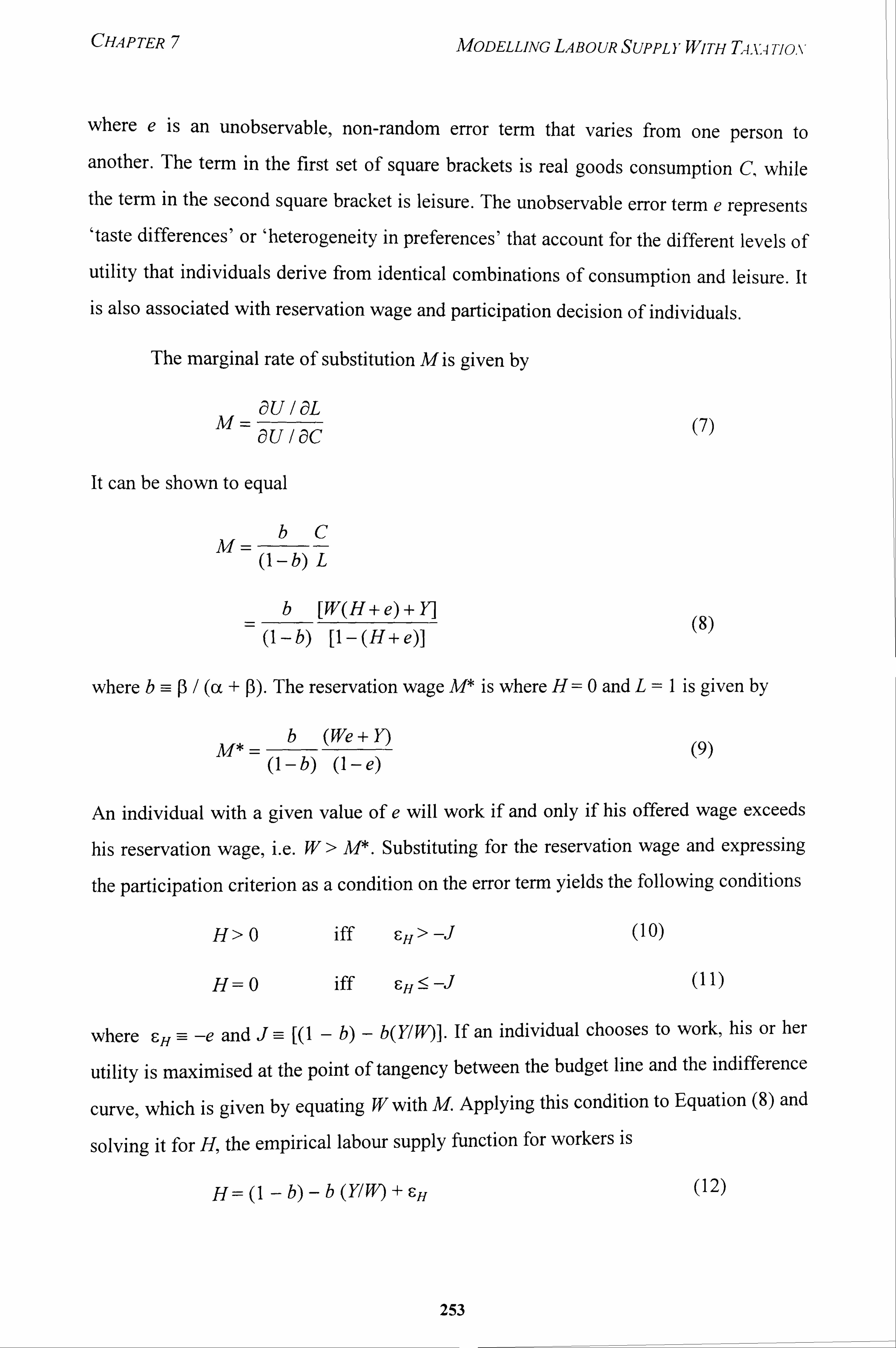
CHAPTER 7 MODELLjNG LABOUR SUPPL YWiTH T4X4 TION

where e is an unobservable, non-random error term that varies from one person to

another. The term in the first set of square brackets is real goods consumption C while the term in the second square bracket is leisure. The unobservable error term e represents 'taste differences' or 'heterogeneity in preferences' that account for the different levels of utility that individuals derive from identical combinations of consumption and leisure. It

is also associated with reservation wage and participation decision of individuals.

The marginal rate of substitution M is given by

aulaL aulac

It can be shown to equal

bC (1-b) L

b [W(H+e)+I] (8)

(1-b) [1-(H+e)]

where b =- p/ (cc + P). The reservation wage M* is where H=0 and L=I is given by

b (We + Y) (I - b) (I - e)

(9)

An individual with a given value of e will work if and only if his offered wage exceeds

his reservation wage, i. e. W> M*. Substituting for the reservation wage and expressing

the participation criterion as a condition on the error term yields the following conditions

H>O iff 6H > -j (10)

H=O iff 6H ýý -j (11)

where - -e and J= [(I - b) - b(Ylffý]- If an individual chooses to work, his or her 6H ==

utility is maximised at the point of tangency between the budget line and the indifference

curve, which is given by equating W with M. Applying this condition to Equation (8) and

solving it for H, the empirical labour supply function for workers is

-b)-b (y/ffý + EH (12)

253

CHAPTER

whereF-H: -ý -e for all positive values of H.

MODELLING LABOUR SUPPLYWJTH TA-v. -i Tio, v

The incorporation of the error term in the utility function has made it possible to derive the threshold condition for participation, as given 'by Equation (10) and Equation (11). Based on the values of W and Y, the analyst can never be sure if an individual

chooses to work or not since his/her decision would also depend on his/her 'inclination

towards work', as given by F- H. The individual will participate if his or her 6H is

sufficiently large and exceeds -[(I-b) - b(Y/ffý], or if the value of the right-hand side of the equation becomes smaller than F, Has a result of an' increase in real wage. An

individual would choose not to work whenc H< -[(I-b) - b(Ylffý].

4.1 Participation Equation

Initially, let us assume that we observe the real wage rate W for all individuals in

the population, including non-workers. To derive the probability that a given individual i

will work, we further assume that F, Hhas a mean of zero, has a standard deviationOf cTH,

and is normally distributed in the population as a whole. This implies that the

standardised normal variable F-Hi ICYHhas a mean of zero and a variance of 1. Given the

assumption of the population distribution of FHj, the probability that the individual will

work is given by

Pr [i works] = Pr I(F-Hi ICYH) ýý* ( -ji / CFH)l

00, ff (t)dt =I- F(-Ji / (TH)

Ji /all

where Ji =I-b- b(Y/W), F-H =-e for all positive values of H, f is the standard normal

density function, and F is the cumulative normal density function. The cumulative

normal density function F(-Ji ICFH) gives the proportion of those who are not working.

Given a sample of N individuals of whom k are observed working, the likelihood

function for a sample of individuals in terms of employment status (working or not

working) is given by

254

CHAPTER

Or in full

MODELLING LABOUR SUPPLYWITH T-1, V, 4 TION

jiN

I-F - fl F

GH _i=k+l_

H (14)

N k (I - b) by+b Yj L=fl I-F -+ cy xFj F- i=l Cy HHi i=k+i H 17 H

I

Equation (14) is the standard probit likelihood function which is the product of the

probability of observing k individuals working and the probability that (N-k) individuals

are non-workers, given their respective values of Y and W. The two parameters of bIGH

and (I -b)/aHcan be estimated by maximising the likelihood function with respect to

b/(THand (I - b) ICTH.

As discussed in the earlier chapter, there is a problem with using real wage in the

labour supply model. Wages are only available for those who work but not for the non-

workers. Estimating hours of work using the data based on workers, with the values of

non-workers set to zero, would create a misspecifi cation problem. On the other hand,

excluding non-workers from the sample to estimate hours of work creates a sample

selection bias problem. Even the remedy that had sometimes been adopted, that is, by

deriving the impute wages based on the least-squares estimate of the wages for workers

and use the imputed wages in place of W, would give rise to potential selectivity bias

problem.

Heckman (1974,1976) addresses this problem by adopting the 'proportionality'

hypothesis in which hours of work are taken to be proportional to the difference between

the real wage W and the reservation wage M* whenever W>M* and zero otherwise. The

model is

Wi =A+ F-wi

am* + cm* Yi + dm* Zi + Emi* i

Hi = b(Wi - Mj*) == a+ bWj + cYj + dZi - bE; mi* (17)

if and only if Wi > Mj*

255

CHAPTER MODELLiNG LABOUR SUPPLYWITH Ti. V, 4Tio. \,

Hi =0 if and only if Wj:! ý Mj* (18)

where a= -baAf*, c= -bcm*, d= -bdm*, W, is real wage, M* is reservation wage, X, and Zi are observable variables, Yj is non-labour income, and Hi is hours of work. The participation equation implied by equations (15)-(18) is

Pr [i works] = Pr [Wi > Mi*]

= Pr [yXi + F, kvi > am* + cm* Yi + dm* Zi + Emi* ]

= Pr [cwj - E; mi* > -JI]

where Ji = yXi - (am* + cm* Yj + dm* Zj). Let us defineF -Di (6wi

- Fmi*) as the difference

between two normally distributed random variables with variances cy 2w

and cy 2m

and with

a covariance awm. Accordingly, F-Di is normally distributed with mean zero and variance

CF 2D=

CY 2W+

(7 2M-

2(Twm.

As before, the parameters of the participation function can be estimated by using

probit likelihood function on the set of workers and non-workers. Assuming a set of N

individuals of whom k are working, the likelihood function is given as follows

kN

L I[I - F(-Jj 1 CYDA

11 F(-Jj 1 CYD

i=l i=k+l

where Ji = yXj - am* - cm*Y, - dm*Zi. This approach replaces W for which data are

usually available for workers only with variables on the right hand side of Equation (15).

4.2 Wage Equation

The purpose of estimating the participation function is to form a measure of k so that it

could be used to estimate the parameters of the wage equation via selection bias-

corrected regression. Using results well known in the literature (see Heckman, 1979:

156) and applying it to the wage equation, we have

E [F-wi 1 FHi > -JA = (cy wH ICYH) 4

f (-Ji / CFD) (20)

I-F(-Jilcyj))

256

CHAPTER 7 MODELLjNG LABOUR SUPPL YWITH T4-Y, 4 Tiav

where f and F are the probability density function and the cumulative distribution function, respectively, for the standard normal random variable, and /ki is the inverse of Mills' ratio, which is the ratio of the ordinate of a standard normal to the tail area of the distribution. The estimated ý computed from the probit parameters from Equation (19)

are used with Xi to estimate a selection bias-corrected regression for the wage equation using data on workers. The wage equation is given by

Wi =A+ Zý +L)i (21)

where ui is a mean-zero random error term, z is an estimate of the. ratio cTWD ICTD, and CFwD

is the covariance between cwi and F-Di (ýE: Wi - 6mi*). The computations used in the

'Heckit' estimation procedure, which is based on the method of moments and consistent

estimationsl are discussed in Heckman (1979) and Greene (1981).

4.3 Hours o Work Equation )f

The estimation of the wage equation parameters provides the means of getting

around the endogeneity problem of net wages in the hours of work equation to be

estimated in the next stage. The expected value of hours worked among people who work

is as follows

E [Hi I Wi > Mi*] =E [Hi I (F-Di IC7D) > (-Ji ICYD)l

= aH+ bHyXi + CHyi+ dHZ, +E 19Hi + bHEwi 1 (FDi /CYD) > (-ji ICYD)]

= aH + bH7Xi + CHyi +dHZi + RCYHD ICYD)+ bf, (cywD /CYD)l Iýli

where

cTHD= covariance between 6Hj and6Di (which is equal to Fwi - Fmi*)

(YwD = covariance between E; wi and F-Di

ý= -j 1(3D) I[ I -F(-Ji

1C7D)l 'i

Ji = yXi - (am* + cm* Yi + dm* Zi)

257

CHAPTER MODELLiNG LABOUR SUPPLY WITH TAXA TIO, v

In this stage of the estimation procedure, the equation for the selection bias- corrected regression on those who work is

Hi -aH +bHWi +cHY, +diZi +aXi +u, (22)

The fitted wage is the instrumental variables measure of W and computed from A

Wi = yXi , where the ̂ are the estimated parameters in Equation (2 1

For our estimations in Section 6, we have adopted a simple model to estimate hours of work equation for both males and females where the spouse's effect on an individual's labour supply is mainly through his or her non-labour income. While we

realise that this individual-based model may have some limitations (since one could

possibly consider the couple's leisure as being complementary or the cross- substitution

effect of the spouse's wage rate), this approach has the advantage of being relatively

straightforward, its results are easy to interpret, and it does not require restrictions to

ensure household equilibrium. In the literature, there are more complex approaches to

model family making. However, there is no consensus on best to model family labour

supply since models of this nature always involve some degree of trade-offs.

5. TAXES AND LABOUR SUPPLY

The basic labour supply model can be extended to incorporate taxes. From Equation (2),

the budget constraint in the absence of taxes and transfers could be written as

Y+ WH= C (23)

With the imposition of taxes, the individual. bears a tax liability A, which is a function of

property income Y and earnings E, the product of hours of work and wage rate. The

budget constraint after taxes is

Y+ WH- A(Y, WH) =C (24)

The tax liability increases with property income and earnings. Hence, the first order

conditions are given by

8A/5 Y --7-: T>

258

CHAPTER

6A/8E =- '7E

MODELLING LABOUR SUPPLYWITH T4. v4 TION

where T I, is the marginal tax rate on property income andTEis the marginal tax rate on

earnings. Under normal circumstances, the marginal tax rate is assumed to lie between 0

and 1, i. e. 0"Y, E "ý' I-

In a progressive tax system, the rise in non-labour income and earnings will shift

an individual into higher marginal tax brackets. The second order conditions are as follows:

22 6 A18Y =- -cyy >0

62 A/6E2 'UEE >0

62 AIME -= 82 Al6E8Y-= 'CEYýý' 0

As an individual increases his hours of work, his tax liabilities will increase along with

his earnings. The net earnings from an additional hour of work is given by

(6E16H)-(6A16H) = (6E16H)-[(6A16E)(8E16H)]

--::: W 'CJV: -- 0 (25)

where co- (1_'ýE)W'Sthe after-tax or net real wage rate, which is the slope of the budget

constraint and represents the opportunity cost of one hour of leisure.

As mentioned in the earlier chapter, the concept of virtual income is widely used

in empirical studies on taxation as a device for linearising the convex budget set. In

formulating virtual income, let the net wage (o gives slope of the linearised budget

constraint at the individual's labour supply maximum. The individual's adjusted property

income y is implicitly defined by the following relationship:

+ coH= C (26)

C- (oH

from (24) Y+ WH- A=C

Y=Y+WH-A-o)H

259

CI14PTER

Since (o (1 -'IE)W

Therefore, virtual income is

Y-(A-'UEWH)

MODELLiNG LA BO UR SUPPLYWITH T4, v 4 Tim,

(27)

whereTEWH is tax paid on earnings, A is tax liability, and C is consumption.

260

CHAPTER 7 MODELLjAiG LABOUR SUPPLYWITH T4x 4 Tiox

6. ESTIMATION RESULTS

We undertake several estimations on hours of work for both males and females. The baseline estimation is first performed in three stages for the whole sample of married couples within the 20-54 years age group. Next, alternative estimations are performed to determine the extent to which the results differ from the baseline estimations. The four

categories of alternative estimations are: (a) hours of work without instrumental

variables, (b) three stage estimation for those working between 25-60 hours a week, (c)

pre-tax hours of work estimation, and (d) regressions by subgroups of occupation,

education and employment category.

1 Baseline Participation Equation

The baseline model is estimated in three stages in order to derive the hours of

work equation for males and females in the prime age group. In the first stage, the

parameters for the participation equations 4 for males and females are derived using the

probit estimation procedure.

1.1 Male

Potential work experience (EXPRC) is a measure of the number of years worked

after leaving school or after the age 15, whichever comes later. This variable is estimated

in its quadratic form, that is, experience and experience squared. For a graphic

presentation of the two coefficients, the male participation equation in Table 7.6 is

plotted in terms of its standard normal density function. As shown in Figure 7.2 and

Figure 7.3, the likelihood of participation (which varies from 0 to 1) is on the vertical

axis and different years of experience is on the horizontal axis. The mean values are used

4 In the literature, the term 'labour supply equation' can either refer to the probability of participation

equation or hours of work equation. To avoid confusion, we refrain from referring to the participation

equation as the labour supply equation.

261

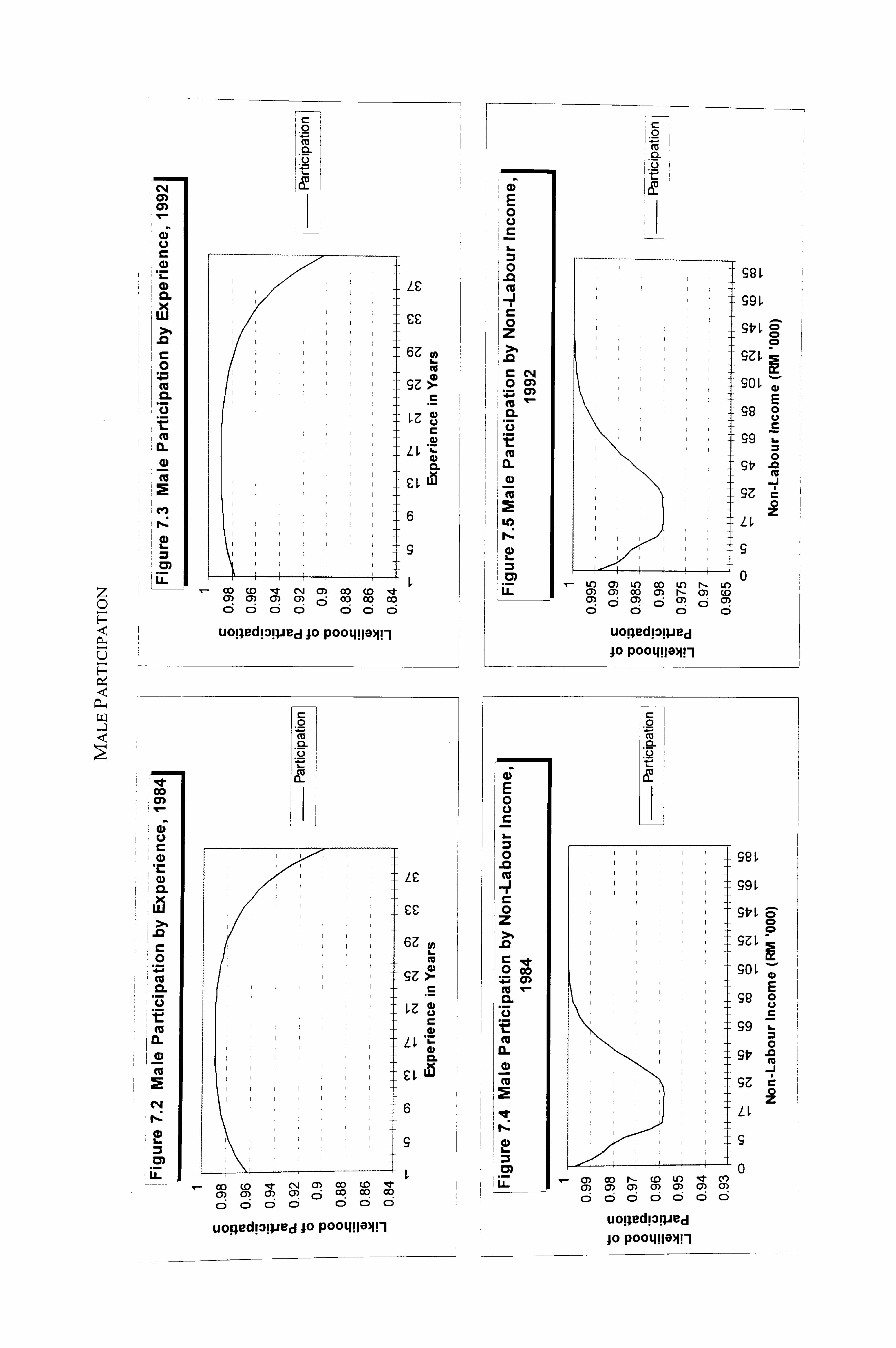
Lij . -j

C',

HH C%4

LU

. 92

i, 0

16.

!M FL

Iý co

4)

CL

0

m

:ý -Zi

cm

ý (T

LC

cc

6Z

9z

ý 40,

C, LV

cIt

6

co (D It 0) co (D it 0) 0) 0) Clý 6 Oý CR CR C) CD C) C) C) C) C)

uolledlol: pBd 10 P004! 10)1! -l

C: 0

Q-

Ll

LC

cc

6Z m

9z >T

LZ

LL CL

CL Ul

6

CC) (C) V, (14 0) CC) (0 Iril 0ý 0) C3) CY) C5 cc! oq cc! ci ci ci ci C) C) C)

uopedlOlVed 10 POOMOV-1

ho : a-

C. ) r

0

C 0

z

C C4

.2 CY) CL

CL

ý e! I cm

L

99L

9

90L

ge

99

9z

LL

i- -4 i0 U') cy) LO co U') rl_ LO

0) 0) 00 cr) rl_ a) (D Cý ci 0ý ci Cý ci Cý C) C) C) C)

uoiled! 31: Pled 10 POOMOTI

a; E 0

0 z

C 0 co CL

.5

it tv

c (o

99ý

9t, ý cl CD 9ZL

90L (D E

98 00

99

9z

LL

0 CY) co r-- (. C) ce)

cý CT) (7) CY) CY) 0) CD

ci 666 ci ci 6

uoljedl3l: PRd 10 P004HOTI

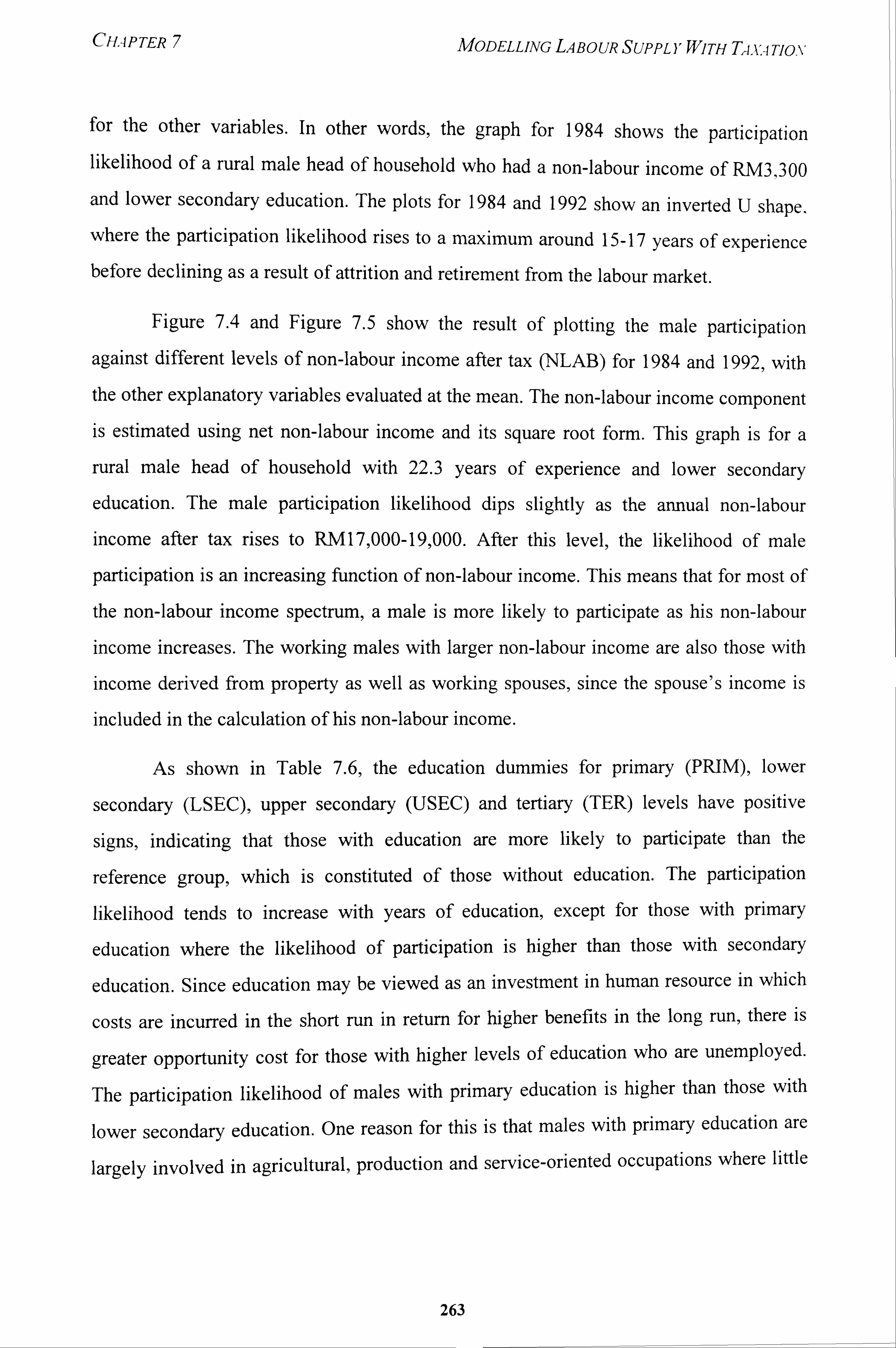
CHAPTER 7 MODELLiNG LABOUR SUPPLYWITH Ti, k, -i Tio, %'

for the other variables. In other words, the graph for 1984 shows the participation likelihood of a rural male head of household who had a non-labour income of RM3,300

and lower secondary education. The plots for 1984 and 1992 show an inverted U shape, where the participation likelihood rises to a maximum around 15-17 years of experience before declining as a result of attrition and retirement from the labour market.

Figure 7.4 and Figure 7.5 show the result of plotting the male participation

against different levels of non-labour income after tax (NLAB) for 1984 and 1992, with the other explanatory variables evaluated at the mean. The non-labour income component

is estimated using net non-labour income and its square root form. This graph is for a

rural male head of household with 22.3 years of experience and lower secondary

education. The male participation likelihood dips slightly as the annual non-labour income after tax rises to RM17,000-19,000. After this level, the likelihood of male

participation is an increasing function of non-labour income. This means that for most of

the non-labour income spectrum, a male is more likely to participate as his non-labour

income increases. The working males with larger non-labour income are also those with

income derived from property as well as working spouses, since the spouse's income is

included in the calculation of his non-labour income.

As shown in Table 7.6, the education dummies for primary (PRIM), lower

secondary (LSEQ, upper secondary (USEQ and tertiary (TER) levels have positive

signs, indicating that those with education are more likely to participate than the

reference group, which is constituted of those without education. The participation

likelihood tends to increase with years of education, except for those with primary

education where the likelihood of participation is higher than those with secondary

education. Since education may be viewed as an investment in human resource in which

costs are incurred in the short run in return for higher benefits in the long run, there is

greater opportunity cost for those with higher levels of education who are unemployed.

The participation likelihood of males with primary education is higher than those with

lower secondary education. One reason for this is that males with primary education are

largely involved in agricultural, production and service-oriented occupations where little

263

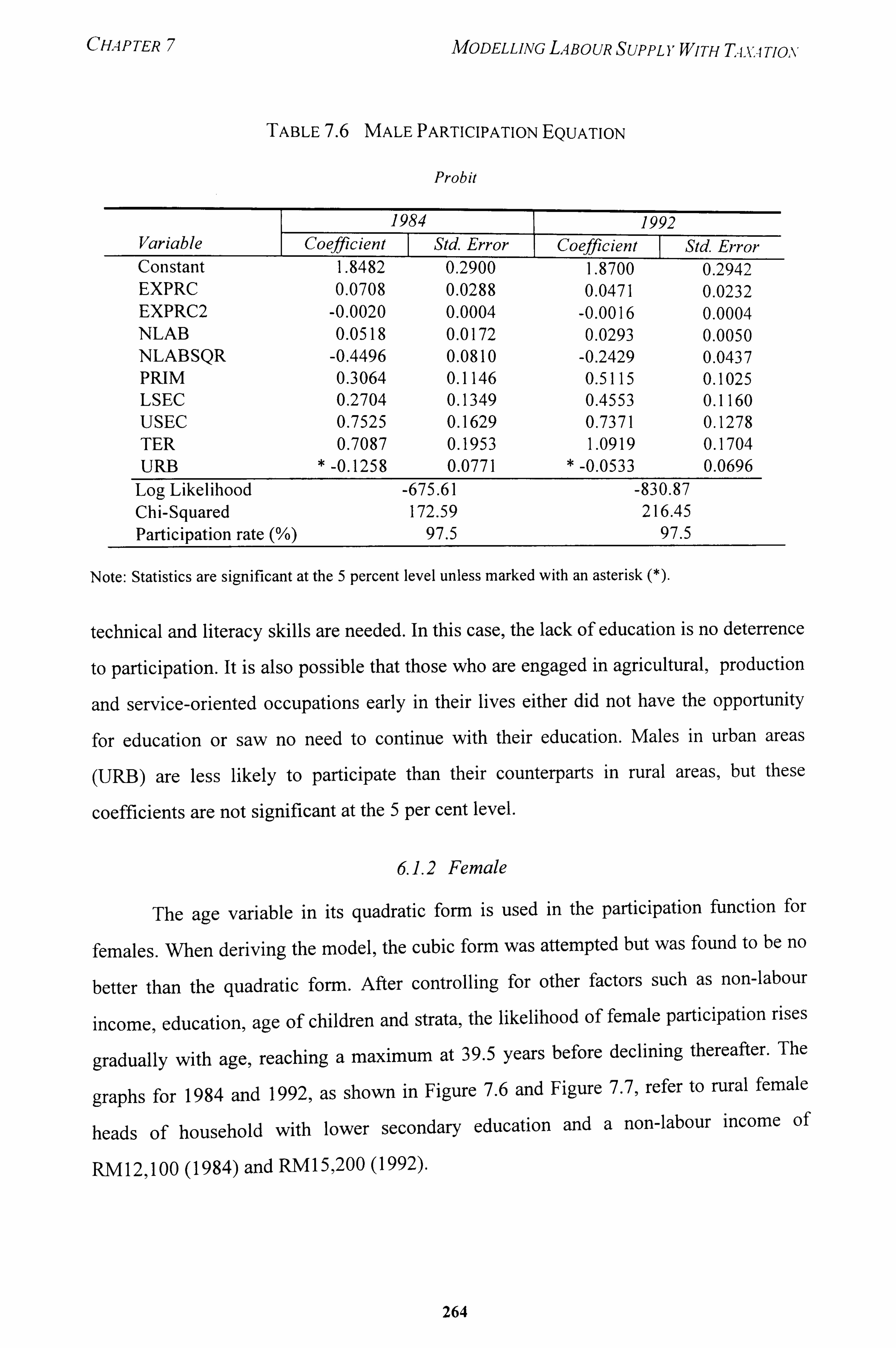
CHAPTER 7 MODELLiNG LABOUR SUPPL YWITH T4-VA TION

TABLE 7.6 MALE PARTICIPATION EQUATION

Probit

1984 1992 Variable Coefficient Std. Error Coefficient Std Error Constant 1.8482 0.2900 1.8700 0.2942 EXPRC 0.0708 0.0288 0.0471 0.0232 EXPRC2 -0.0020 0.0004 -0.0016 0.0004 NLAB 0.0518 0.0172 0.0293 0.0050 NLABSQR -0.4496 0.0810 -0.2429 0.0437 PFJM 0.3064 0.1146 0.5115 0.1025 LSEC 0.2704 0.1349 0.4553 0.1160 USEC 0.7525 0.1629 0.7371 0.1278 TER 0.7087 0.1953 1.0919 0.1704 URB * -0.125 8 0.0771 * -0.0533 0.0696

Log Likelihood -675.61 - 830.87 Chi-Squared 172.59 216.45 Participation rate 97.5 97.5

Note: Statistics are significant at the 5 percent level unless marked with an asterisk (*).

technical and literacy skills are needed. In this case, the lack of education is no deterrence

to participation. It is also possible that those who are engaged in agricultural, production

and service-oriented occupations early in their lives either did not have the opportunity

for education or saw no need to continue with their education. Males in urban areas

(URB) are less likely to participate than their counterparts in rural areas, but these

coefficients are not significant at the 5 per cent level.

6.1.2 Female

The age variable in its quadratic form is used in the participation function for

females. When deriving the model, the cubic form was attempted but was found to be no

better than the quadratic form. After controlling for other factors such as non-labour

income, education, age of children and strata, the likelihood of female participation rises

gradually with age, reaching a maximum at 39.5 years before declining thereafter. The

graphs for 1984 and 1992, as shown in Figure 7.6 and Figure 7.7, refer to rural female

heads of household with lower secondary education and a non-labour income of

RM 12,100 (1984) and RM 15,200 (1992).

264

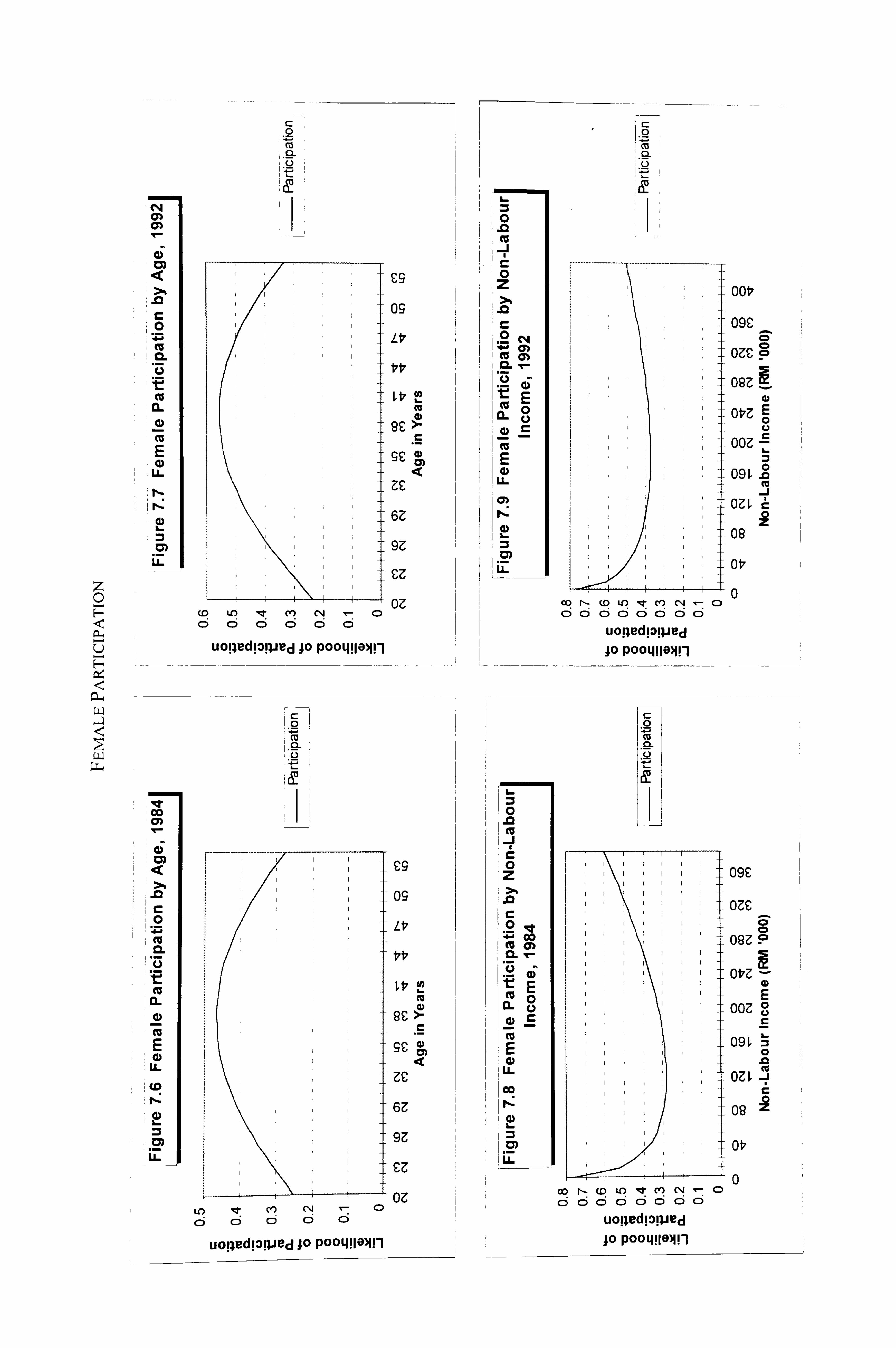
7- 0

ra. u

LLI

C*4 (7) 0)

co

CL

E U-

Q

i7L

C 0

0

£g

09

Lt,

t't,

ýt1 au-)

6Z

93

U

0

0

ýz

C

1.2 *a i CU i CL

e4 CY) CD : 2-L)

CL E 0

E (D

U.

al

21 U-

(D to 'IT c1r) C14 V-- C) c; ci ci ci ci C=i

uolledl3l: PL'd 10 POOMOV-1

1 qe ý 00

:. 0)

>b

C 0

CL

(D

E U-

0o i cc

os

tt,

16.

i cm

6Z

9z

oz C%i

CD czi c5 ci c: i

UOl; ud1311Jed 10 POOLI! IOM! «l

0 . 92

0 Z

J2

.0 *-0

LL

c

0

oot7

09C

ozc

o9zl

otz E 1

ooz

0 I 09L

OZL

08

ot,

0 co r- (0 U') IT C") CN C) C) C) C) C) C) 0 C) C)

uolledl: )I: PBd 10 POOMOVI

c

09C

On

o9z p

OtZ -

ON

oqý 0 .0

ou 3 C

08

OV

0 co r- (D U') NT ce) CN ý C)

ci C) ci o ci ci uolledl0l: PL'd 10 P004! 181! 1

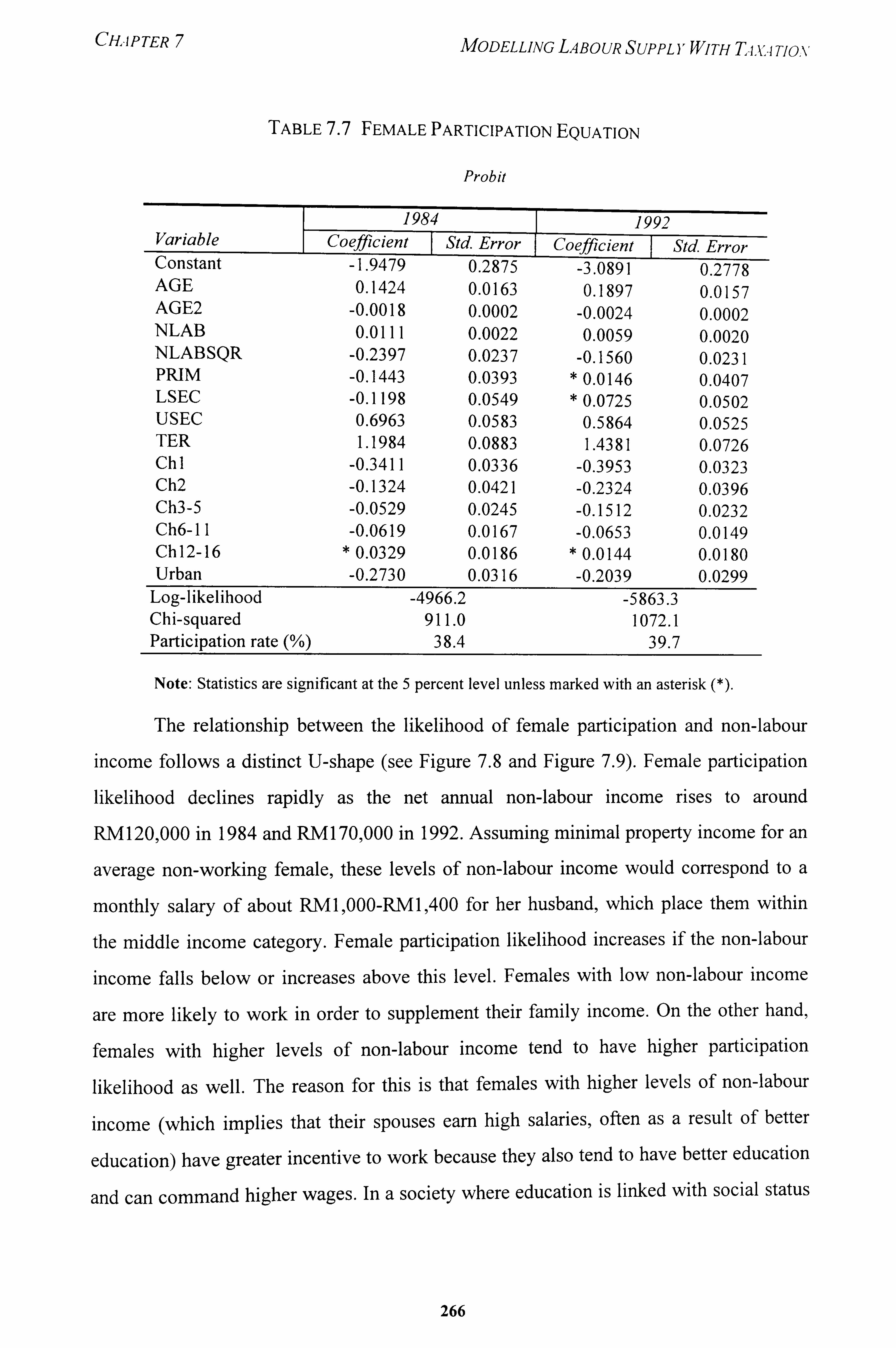
CHAPTER 7 MODELLING LABOUR SUPPLYWITH T-i. v. i Tiox

TABLE 7.7 FEMALE PARTICIPATION EQUATION

Probit

1984 1992 Variable Coefficient Std Error Coefficient Std. Error Constant -1.9479 0.287ý_ -3.0891 0.2778 AGE 0.1424 0.0163 0.1897 0.0157 AGE2 -0.0018 0.0002 -0.0024 0.0002 NLAB 0.0111 0.0022 0.0059 0.0020 NLABSQR -0.2397 0.0237 -0.1560 0.0231 PRIM -0.1443 0.0393 * 0.0146 0.0407 LSEC -0.1198 0.0549 * 0.0725 0.0502 USEC 0.6963 0.0583 0.5864 0.0525 TER 1.1984 0.0883 1.4381 0.0726 Chl -0.3411 0.0336 -0.3953 0.0323 Ch2 -0.1324 0.0421 -0.2324 0.0396 Ch3-5 -0.0529 0.0245 -0.1512 0.0232 Ch6-1 1 -0.0619 0.0167 -0.0653 0.0149 Ch 12-16 0.0329 0.0186 0.0144 0.0180 Urban -0.2730 0.0316 -0.2039 0.0299

Log-likelihood - 4966.2 -5863.3 Chi-squared 911.0 1072.1 Participation rate 38.4 39.7


The relationship between the likelihood of female participation and non-labour

income follows a distinct U-shape (see Figure 7.8 and Figure 7.9). Female participation

likelihood declines rapidly as the net annual non-labour income rises to around

RM 120,000 in 1984 and RM 170,000 in 1992. Assuming minimal property income for an

average non-working female, these levels of non-labour income would correspond to a

monthly salary of about RMI, 000-RMI, 400 for her husband, which place them within

the middle income category. Female participation likelihood increases if the non-labour

income falls below or increases above this level. Females with low non-labour income

are more likely to work in order to supplement their family income. On the other hand,

females with higher levels of non-labour income tend to have higher participation

likelihood as well. The reason for this is that females with higher levels of non-labour

income (which implies that their spouses earn high salaries, often as a result of better

education) have greater incentive to work because they also tend to have better education

and can command higher wages. In a society where education is linked with social status

266

CHAPTER 7 MODELLiNG LABOUR SUPPLYWITH Tq. v. 4 Tiox

and earning power, better educated women tend to marry husbands who have either an equivalent or higher educational attainment.

As shown in Table 7.7, the coefficients of the education dummies for 1984 are negative for primary and lower secondary education and positive for upper secondary and tertiary education. In 1992, the coefficients for all the education dummies are positive though the coefficient for PRIM and LSEC are insignificant at the 5 per cent level. The likelihood of female participation increases at USEC and TER for both the

years. The children dummies refer to women having at least a child at or below the age I (CHI), at the age 2 (CH2), as well as between ages 3-5 years (CH3_5), 6-11 years (CH6_1 1) and 12-16 years (CH12-16). As expected, young children have a strong disincentive effect on a woman's participation, especially for children below 5 years old. Children at this age make strong demands on their mother's time, care and attention. The disincentive effect becomes less pronounced with older children. In fact5 women with

older children above the age of 12 years are more likely to work since children at these

ages can help out with household chores.

As with the males, the urban dummy for females has a negative sign, implying

higher participation for rural females. The higher likelihood of female participation in the

rural areas is because females in the rural areas are able to perform their household

activities alongside working in the farm, which are often family owned. Unlike urban

jobs, it is much harder to distinguish participation from non-participation in the case of

agricultural occupations because of the greater degree of disguised unemployment and

underemployment. In addition, the inflow of rural migrants to urban areas in search of

jobs contribute to a higher rate of urban unemployment, and hence the lower

participation likelihood for urban fernales.

62 Instrumentingfor Wage and Virtual Income

6.2.1 Baseline wage equation

The wage equation is estimated as an instrument for the hours of work equation

in order to overcome the problem of endogeneity. The dependent variable, net wage, is

267

CHAPTER 7 MODELLiNG LABOUR SUPPLYWiTH Ti, V4 TION

expressed in log form, thereby giving a semi-logarithmic relationship to the model. The

semi-log specification was found to be appropriate after trying out several model specifications in the initial stage of the regression runs.

Two alternative sets of variables are used for the baseline wage equation. The

first alternative (ALTI) assumes that unlike wage after tax which is clearly related to

hours of work put in by an individual, gross wage rate and non-labour income are independent of the amount of hours worked. This is consistent with the view that in a

competitive market for homogenous labour, individuals confront a fixed market wage

offer. This assumption is implicit in the models by Flood and MaCurdy (1992) and

Blomquist (1996) who used gross wage rate and non-labour income in some of their

models to instrument for the net wage rate in Sweden. The independent variables in the

baseline wage equation are wage, wage square root (WAGESQR), non-labour income

(NLAB), non-labour income square root (NLABSQR), experience or age, and lamda to

adjust for selection bias.

In the second alternative (ALT2), we relax the exogeneity assumption for the

instrumental variable estimators by excluding gross wage and non-labour income from

the wage equation. This alternative uses socio-demographic variables as instruments,

namely, potential work experience or age, potential work experience (or age) squared,

education, occupation, and lamda. Unlike ALTI,, this alternative avoids using gross wage

rate which may be affected by the errors made in measuring the amount of hours

5 worked .

It is interesting to note that Flood and MaCurdy (1992) and Blomquist (1996)

who used the gross wage rate and non-labour income to instrument for the net wage rate

in their models differed in opinion on the relative merits of the instruments. By using

gross wage and non-labour income as instruments (as in our ALT I), Flood and MaCurdy

were able to replicate the results obtained by using maximum-likelihood procedures.

They argued that the 'high' positive value which was derived for the wage rate by

5 The Alternative 2 wage equation parallels the functional form adopted by Mincer (1974) and Becker

(1964) in the human capital earnings function which uses years of schooling and post-schooling

experience.

268

CHAPTER 7 MODELLING LABOUR SUPPLYWITH T4-k, 4 Tio, %,

estimators like IVI was due to the endogeneity of the gross wage rate and nonlabour income. They favoured an estimator like IV2 which takes care of both the endogeneity in the gross wage rate and nonlabour income as well as the endogeneity in net wage rates imposed by non-linear taxes.

Blomquist, on the other hand, argued that it is difficult to test whether the gross wage rate and non-labour income were admissible instruments. However,, when gross wage rate and non-labour income were excluded from the model, his simulations showed that using socio-economic variables as instruments had a serious negative bias for the wage rate coefficient, especially for small samples. The small-sample bias arose because

of the weak correlation between the instruments with the net wage rate. Blomquist

confirmed Flood and MaCurdy's finding that the model with wage and non-labour income variables performed as well as the maximum likelihood method. In his Monte Carlo simulations, he found that the inclusion of wage and non-labour variables produced a small negative bias in the wage rate coefficient when there was a measurement error in

the gross wage rate, which was calculated as labour income divided by hours of work. In

addition, the estimator performed fairly well if the measurement error in the gross wage is additive (Blomquist, 1996: 403). In our regression estimates, we use both alternatives to ascertain if they produce significantly different results, either in terms of the

coefficient estimates obtained or giving rise to a change of signs in the income and

substitution effects.

6.2.1.1 Male

Results of the estimates on the instruments for net wages are given in Table 7.8.

In Alternative I. the adjusted R squared statistics are very high and the F distribution

statistics are very significant. Log net wage has a quadratic relationship with WAGE and

WAGESQR and the very significant t-ratios suggest that wage and wage squared are

good instruments for net wage, assuming that there is no problem with endogeneity. The

coefficients for NLAB are negative and significant at the 5 per cent level for both the

years. The coefficients for the AGE variable, which are used to control for the effect of

age on wage, are negative, while the URB coefficients are positive. It appears that

269

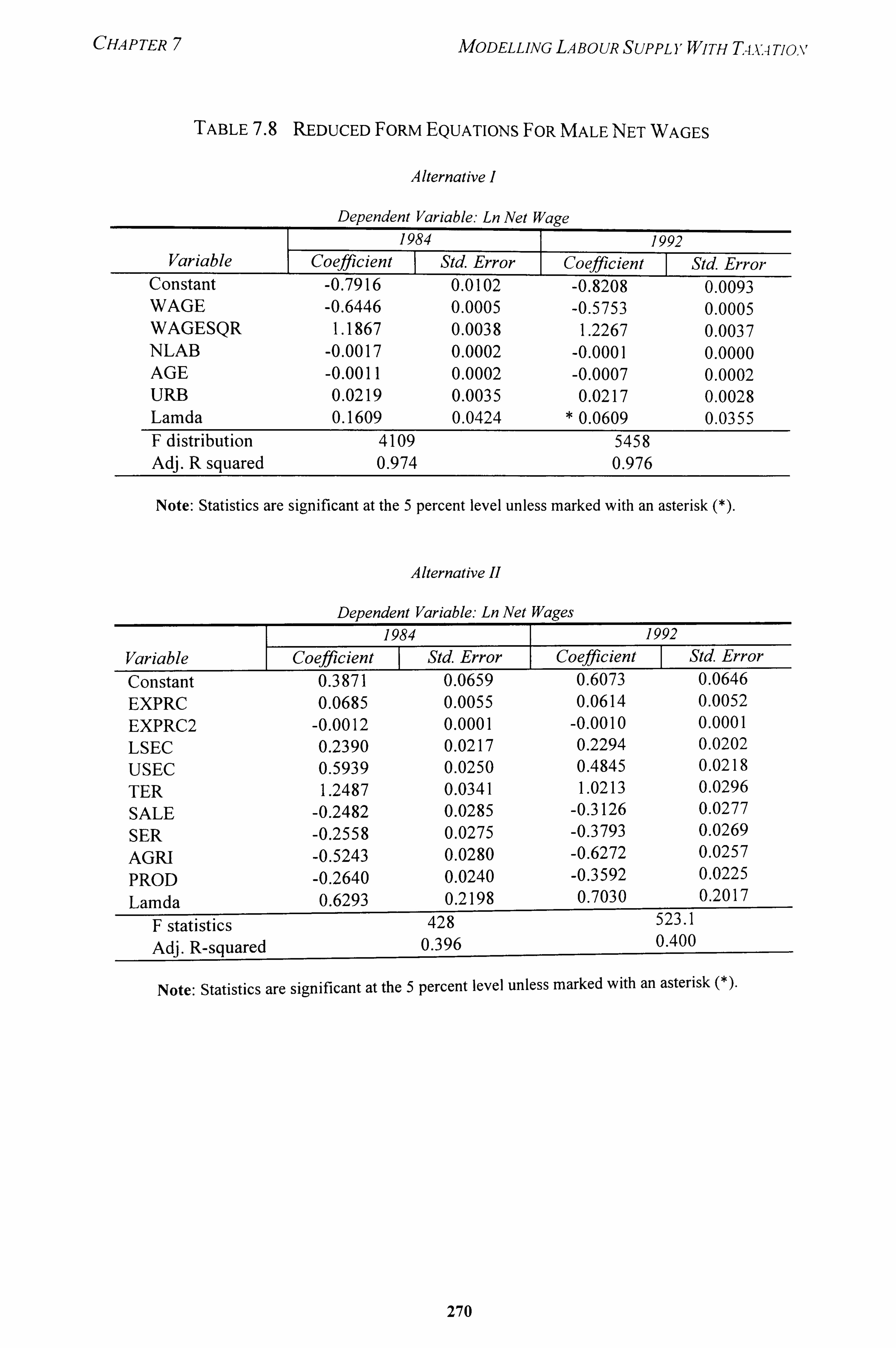
CHAPTER 7 MODELLING LABOUR SUPPLYWITH T4. k. 4 Tio, %'

TABLE 7.8 REDUCED FORm EQUATIONS FOR MALE NET WAGES

Alternative I

Dependent Variable: Ln Net Wage 1984 1992

Variable Coefficient Std. Error Coeffic-i-e-n-t-j Std. Error Constant -0.7916 0.0102 -0.8208 0.0093 WAGE -0.6446 0.0005 -0.5753 0.0005 WAGESQR 1.1867 0.0038 1.2267 0.0037 NLAB -0.0017 0.0002 -0.0001 0.0000 AGE -0.0011 0.0002 -0.0007 0.0002 URB 0.0219 0.0035 0.0217 0.0028 Lamda 0.1609 0.0424 0.0609 0.0355 F distribution 4109 5458 Adj. R squared 0.974 0.976

Note: Statistics are significant at the 5 percent level unless marked with an asterisk (*)

Alternative H

Dependent Variable: Ln Net Wages 1984 1992

Variable Coefficient Std. Error Coefficient Std. Error Constant 0.3871 0.0659 0.6073 0.0646 EXPRC 0.0685 0.0055 0.0614 0.0052 EXPRC2 -0.0012 0.0001 -0.0010 0.0001 LSEC 0.2390 0.0217 0.2294 0.0202 USEC 0.5939 0.0250 0.4845 0.0218 TER 1.2487 0.0341 1.0213 0.0296 SALE -0.2482 0.0285 -0.3126 0.0277 SER -0.2558 0.0275 -0.3793 0.0269 AGRI -0.5243 0.0280 -0.6272 0.0257 PROD -0.2640 0.0240 -0.3592 0.0225 Lamda 0.6293 0.2198 0.7030 0.2017

F statistics 428 523.1 Adj. R-squared 0.396 0.400


270

CHAPTER 7 MODELLING LABOUR SUPPLYWJTH T-i. vq Tim,

although urban males have a lower participation likelihood, those who are working have higher net wages than the rural males. The coefficient for selectivity adjustment 'k is significant in 1984 but not in 1992. The regression equations have highly significant F

statistics and adjusted R squared.

In Alternative 11, the three categories of variables used in the model are years of

post-school work experience, levels of schooling and occupation. All the t-ratios and F

statistics are significant at the 5 per cent level. The adjusted R squared statistics are

moderately high where 40 per cent of the variance of log net wage can be explained by

the variables in the regression. Experience is expressed in quadratic terms, that is,

EXPRC and EXPRC2. Theoretically, this refers to potential experience and acts as a

proxy for the acquisition of human capital. It seems to correspond with the assumption

that investment in human capital declines linearly with time. 6 The inclusion of

experience has been proposed by Mincer (1974) and is considered to be an appropriate

proxy for estimating the returns to human capital (Willis and Rosen, 1979).

Since the level of unemployment among Malaysian males is very low, there is

little problem associated with using the experience variable for the males. EXPRC and

EXPRC2 show the correct sign and are statistically significant. Net wage increases with

years of experience and reaches the maximum at 28.5 years for 1984 and 30.7 years in

1992!, 7 before declining (see Figure 7.10 and Figure 7.11). The charts refer to an average

male with lower secondary education in the reference group occupation. The reasons for

the decline are physical deterioration in strength and health, and the vintage effects.

Workers of an older cohort tend to be less in touch with the modem world and less

amenable to acquire new knowledge and skills compared with those in younger cohorts.

6 For the proof, see Fallon and Verry 0 988: 149-50).

The maximum value of the wage function with respect to experience can be calculated from the

derivatives of the function. For instance, the maximum for 1984 occurs at 0.0685 / (2 x 0.0012) = 28.5

years.

271

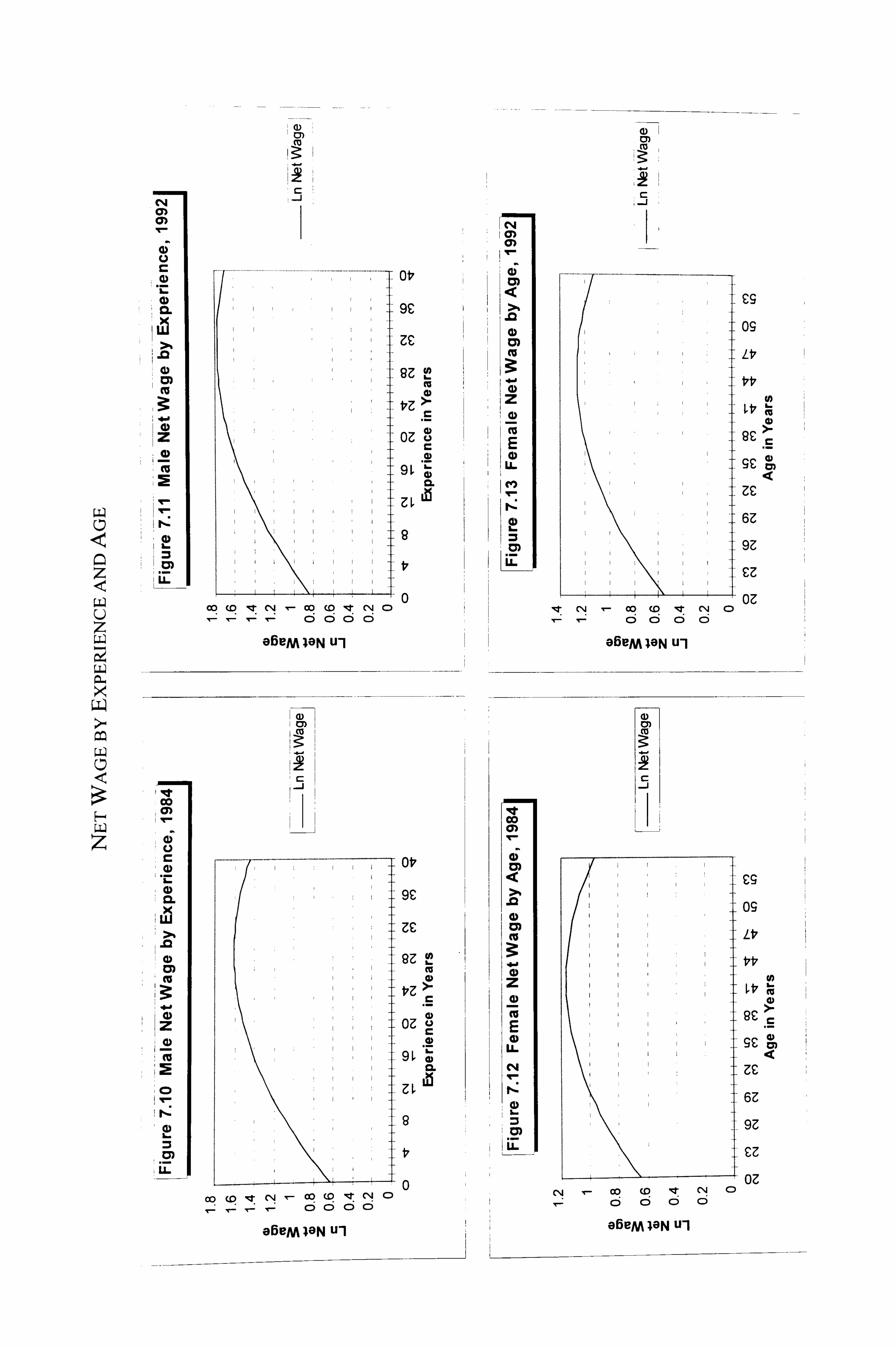
04 CY)

a

iýt;

) LL

co

cl)

I)

-J

04 M C)

-.......... ...... ................. .......... --I1 4) III--

ot, I cr.

9c

IIN cy RZ tlz

oz 2

1 91 CL

co 10 "T CN CO 1.0 11' 04 C) 000 C)

OBUM ION Ul

. 92

, 0)

, CD

(D 16.

ý a) 1 1 c3) i

Ot,

. :: Z£

ez

tlz

111 -- oz 0 A

CL tu

Co Co q- C%j x--- CO (0 e C'4 C) X-- CD C) CD CD

a6eM ION U'l

cl)

C

1 09

s; c

iIU

6Z

9z

III -- cz

oz

(P ll: ý clý C) C) C) C) C

GBBM ION U-1

qe Co 0 Ir-

co

LL

rz

i

os

Lt,

t't,

ýt1

ee s£

U

6Z

9z

n7 CO 'o

cj ci ci ci

OBeM ION U-1

CHAPTER MODELLiNG LABOUR SUPPLYWITH Tiu Tio, v

Education measures the formal acquisition of human capital. In the regression, education dummy variables are used to capture the effect of the level of highest

educational attainment on wages. This coefficient for each dummy variable reflects the return to each level of schooling compared with the reference category of those having

primary or no education. The coefficients are positive and highly significant, which

means that workers with higher education have a clear advantage over those with lower

education in earning higher wages. The coefficients for those with lower secondary

education are 23.9 per cent in 1984 and 22.9 per cent in 1992. This means that the return to lower secondary education is around 24 per cent higher than those with primary or no

education. The return to upper secondary education is more than double that from lower

secondary education, while the return to tertiary education is in turn double that from

upper secondary education. The increasing returns to higher levels of education

corresponds with the studies by Demery and Chesher (1993 on the Malaysian data. 8

Whether the role of education is to augment productivity or used for screening out those

with innate abilities, there is no doubt that employers pay a premium to those who are

better educated.

Occupation is an important factor accounting for the variation in earnings among

workers. The coefficients for the occupational dummies show the net wages of workers

in various occupational groups compared with the reference group, which comprises the

professional, technical, managerial and clerical occupations. Compared with the

reference group, those involved in sales, service and production occupations earn about

25 per cent lower in 1984 and their relative wages were lower in 1992 by 31-38 per cent.

Workers in agricultural occupations saw the worsening of their relative wage which

declined from the level of 52 per cent of the reference group average wage in 1984 to 63

8 This finding on Malaysia differs from Psacharopoulos (1984) who maintains that the private rate of

return to education in developing countries is highest at the primary level and the interest of these

countries are best served by improving the quality of primary education rather than making expensive investments in higher education.

273

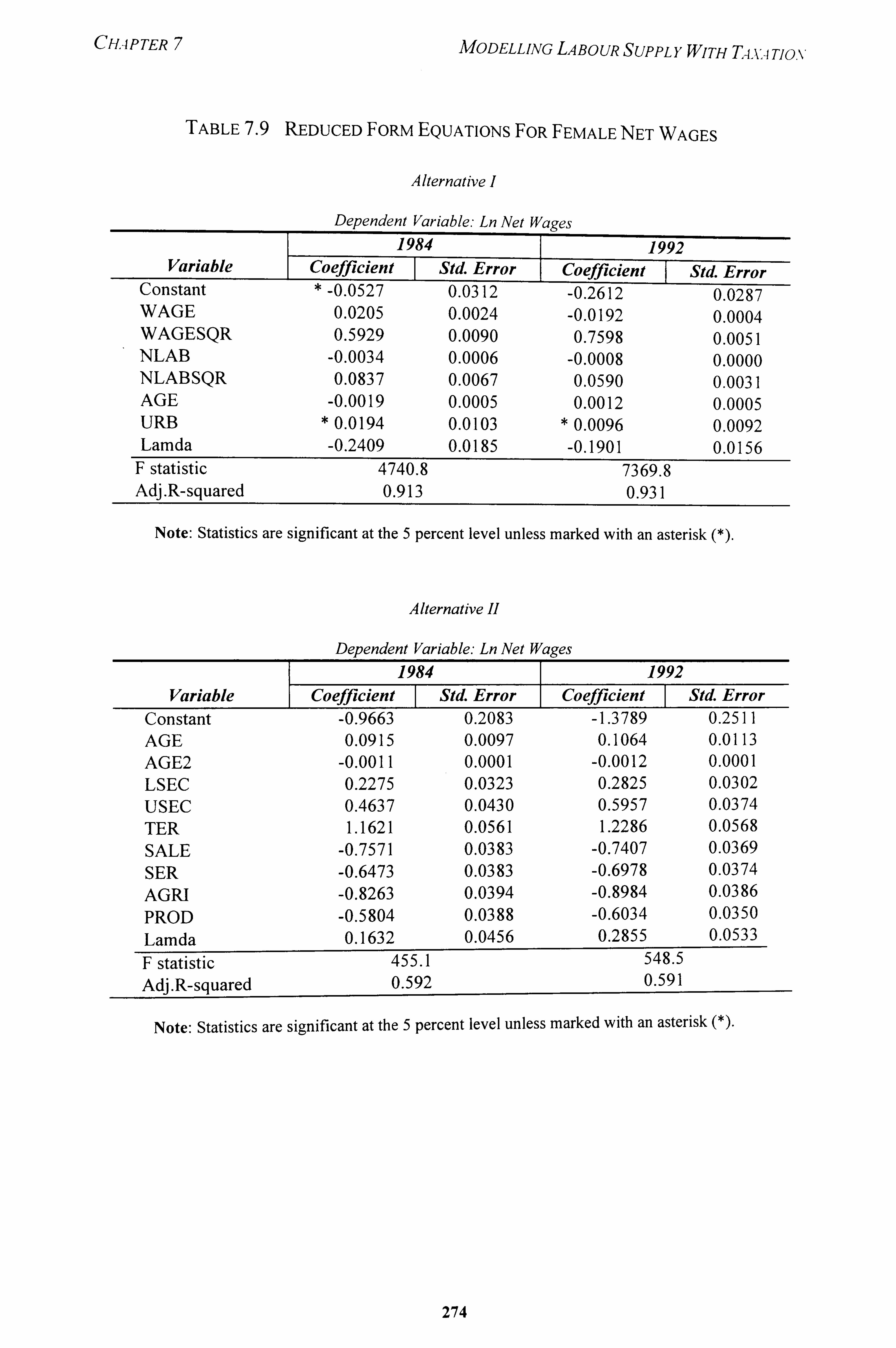
CH-4PTER

TABLE 7.9

MODELLiNG LABOUR SUPPLY WITH T4X-I TION

FD --EDUCED FORM EQUATIONS FOR FEMALE NET WAGES

Alternative I

Dependent Variable: Ln Net Wages

Variable Constant WAGE WAGESQR NLAB NLABSQR AGE URB Lamda

1984 1992 Coefficient Std. Error Coefficient Std. Error

-0.0527 0.0312 -0.2612 0.0287 0.0205 0.0024 -0.0192 0.0004 0.5929 0.0090 0.7598 0.0051

-0.0034 0.0006 -0.0008 0.0000 0.0837 0.0067 0.0590 0.0031

-0.0019 0.0005 0.0012 0.0005 0.0194 0.0103 0.0096 0.0092

-0.2409 0.0185 -0.1901 0.0156 F statistic Adj. R-squared

4740.8 0.913

7369.8 0.931


Alternative H

Dependent Variable: Ln Net Wages 1984 1992

Variable Coefficient Std. Error Coefficient Std. Error Constant -0.9663 0.2083 -1.3789 0.2511 AGE 0.0915 0.0097 0.1064 0.0113 AGE2 -0.0011 0.0001 -0.0012 0.0001 LSEC 0.2275 0.0323 0.2825 0.0302 USEC 0.4637 0.0430 0.5957 0.0374 TER 1.1621 0.0561 1.2286 0.0568 SALE -0.7571 0.0383 -0.7407 0.0369 SER -0.6473 0.0383 -0.6978 0.0374 AGRI -0.8263 0.0394 -0.8984 0.0386 PROD -0.5804 0.0388 -0.6034 0.0350 Lamda 0.1632 0.0456 0.2855 0.0533

F statistic 455.1 548.5 Adj. R-squared 0.592 0.591


274

CHAPTER 7 MODELLiNG LABOUR SUPPLYWITH TAx. 4 Tio, %'

per cent in 1992. The t-ratios for these variables and the coefficient for lamda for 1984 and 1992 are significant at the 5 per cent level.

6.2.1.2 Female

The regression results of the two alternative specifications used for instrumenting net wages are given in Table 7.9. Under Alternative 1, the coefficients for WAGE,

WAGESQR, NLAB, and NLABSQR are highly significant. The AGE coefficients for

1984 and 1992 are significant at the 5 per cent level. The urban dummy variable indicates that the females in urban areas enjoy slightly higher wages than the rural females but these coefficients are not significant.

The model specification for Alternative 11 for the females is similar to that for the

males except that the age and age squared variables are used in the place of the

experience and experience squared variables. The plots of female log net wage by age for

1984 and 1992 are shown in Figure 7.12 and Figure 7.13. The charts refer to an average female with lower secondary education and engaged in the reference group occupation.

Net wage rises gradually as age increases from 20 years to 41 years in 1984 (44 years in

the case of 1992), before declining. The education variables show that the females

receive wage premium for increasing levels of education. In fact, the female wage

increments for education attainments above the primary level in 1992 are even greater

than for the males.

After controlling for age and education, the relative net wages received by

females in the sales, service, and production occupations are equivalent to 60-75 per cent

of the reference occupations average net wage. 9 For females in the agricultural

occupations, their average net wage are even lower at 80-90 per cent of the reference

group wage. The worsening of the relative wages among occupations during 1984-92 is

most marked for agricultural and service occupations. The coefficients on k are

statistically significant which shows evidence of self selection. The adjusted R squared is

59 per cent and the F statistic is highly significant at the 5 per cent level.

9 The reference occupations refer to professional and technical, managerial and administrative, and

clerical occupations.

275

CH. -IPTER 7 MODELLiNG LABOUR SUPPL YWITH T-I. u Tiox

6.2.2 Virtual income

Virtual income is the intercept of the linearised budget set at zero hours of work. Hall (1973), who was one of the first to use the technique to linearise the budget set, treated marginal tax rate and virtual income as exogenous. This can be a problem since virtual income is determined by the level of non-labour income as well as the net wage rate, which in turn depends on the hours worked and marginal tax rates. The linearised budget set is endogenous with respect to hours of work.

Subsequent studies adopted several strategies to overcome this problem of

endogeneity. Rosen (1976) and Hausman and Wise (1976) used the same level of hours

of work for all individuals to derive the marginal tax rate in the construction of net wage

rates and virtual incomes. Layard, Barton and Zabalza (1980) adopted the two-stage least

squares approach. In the first stage, they regressed a dummy variable for taxpayers t on

In W, V and Z. They then used the predicted t instead of the actual t to estimate the hours

of work equation. The instrumental variables approach was used by Johnson and

Pencavel (1982), who replaced the right-hand side variables of the hours of work

equation with their corresponding predicted values from prior regressions on a set of

exogenous variables.

To be consistent with our approach in dealing with the endogeneity of net wages,

we adopt a similar procedure to instrument for virtual income. In the regression equation,

virtual income is regressed against gross wage and non-labour income assumed to be

independent of the amount of hours worked. As shown in Table 7.10, the regression

results of the virtual income equation are highly significant. The high adjusted R-squared

in the regressions for males and females implies that the model came very close to

explaining almost all of the variations in virtual income.

276

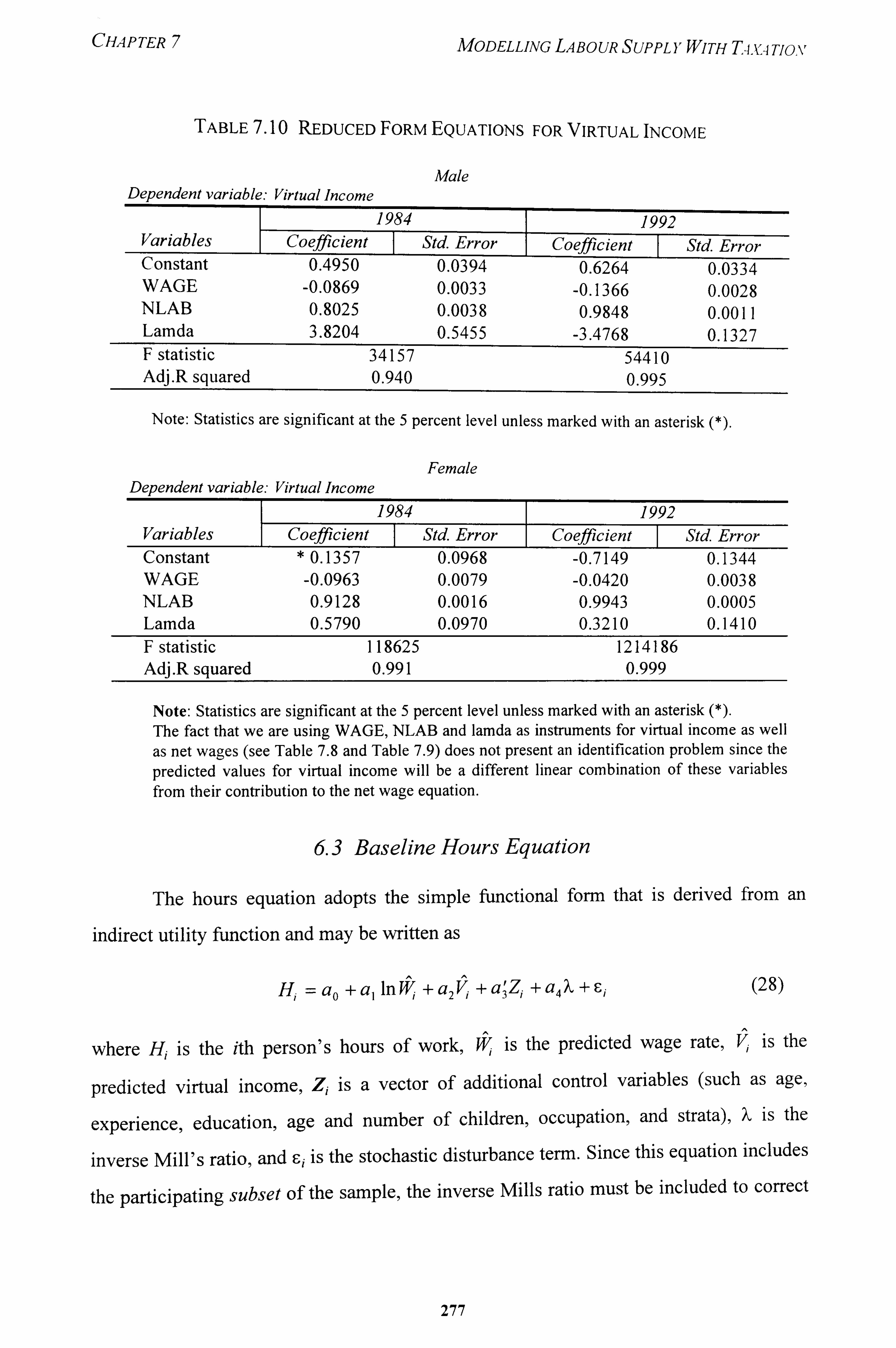
CHAPTER 7 MODELLiNG LABOUR SUPPLYWITH T-i. u Tio, v

TABLE 7.10 REDUCED FORM EQUATIONS FOR VIRTUAL INCOME

Dependent variable: Virtual Income Male

1984 -

1992 Variables Coefficient F Std. Error Coefficient Std. Error Constant 0.4950 0.0394 0.6264 0.0334 WAGE -0.0869 0.0033 -0.1366 0.0028 NLAB 0.8025 0.0038 0.9848 0.0011 Lamda 3.8204 0.5455 -3.4768 0.1327 F statistic 34157 54410 Adj. R squared 0.940 0.995


Female DeDendent variable: Virtual Income

1984 Variables Constant WAGE NLAB Lamda F statistic Adj. R squared

Coefficient * 0.1357

-0.0963 0.9128 0.5790

118625 0.991

Std. Error 0.0968 0.0079 0.0016 0.0970

1992 Co effi cie nPi t

-0.7149 -0.0420 0.9943 0.3210

1214186 0.999

Std. Error 0.1344 0.0038 0.0005 0.1410

Note: Statistics are significant at the 5 percent level unless marked with an asterisk (*). The fact that we are using WAGE, NLAB and lamda as instruments for virtual income as well as net wages (see Table 7.8 and Table 7.9) does not present an identification problem since the predicted values for virtual income will be a different linear combination of these variables from their contribution to the net wage equation.

6.3 Baseline Hours Equation

The hours equation adopts the simple functional form that is derived from an

indirect utility function and may be written as

Wi

Vi +a'Zi +a' ao +a, In +a2 34 'ý' + F' i (28)

where Hi is the ith person's hours of work, W, is the predicted wage rate, Vi is the

predicted virtual income, Zi is a vector of additional control variables (such as age,

experience, education, age and number of children, occupation, and strata), k is the

inverse Mill's ratio, and Ej is the stochastic disturbance term. Since this equation includes

the participating subset of the sample, the inverse Mills ratio must be included to correct

277

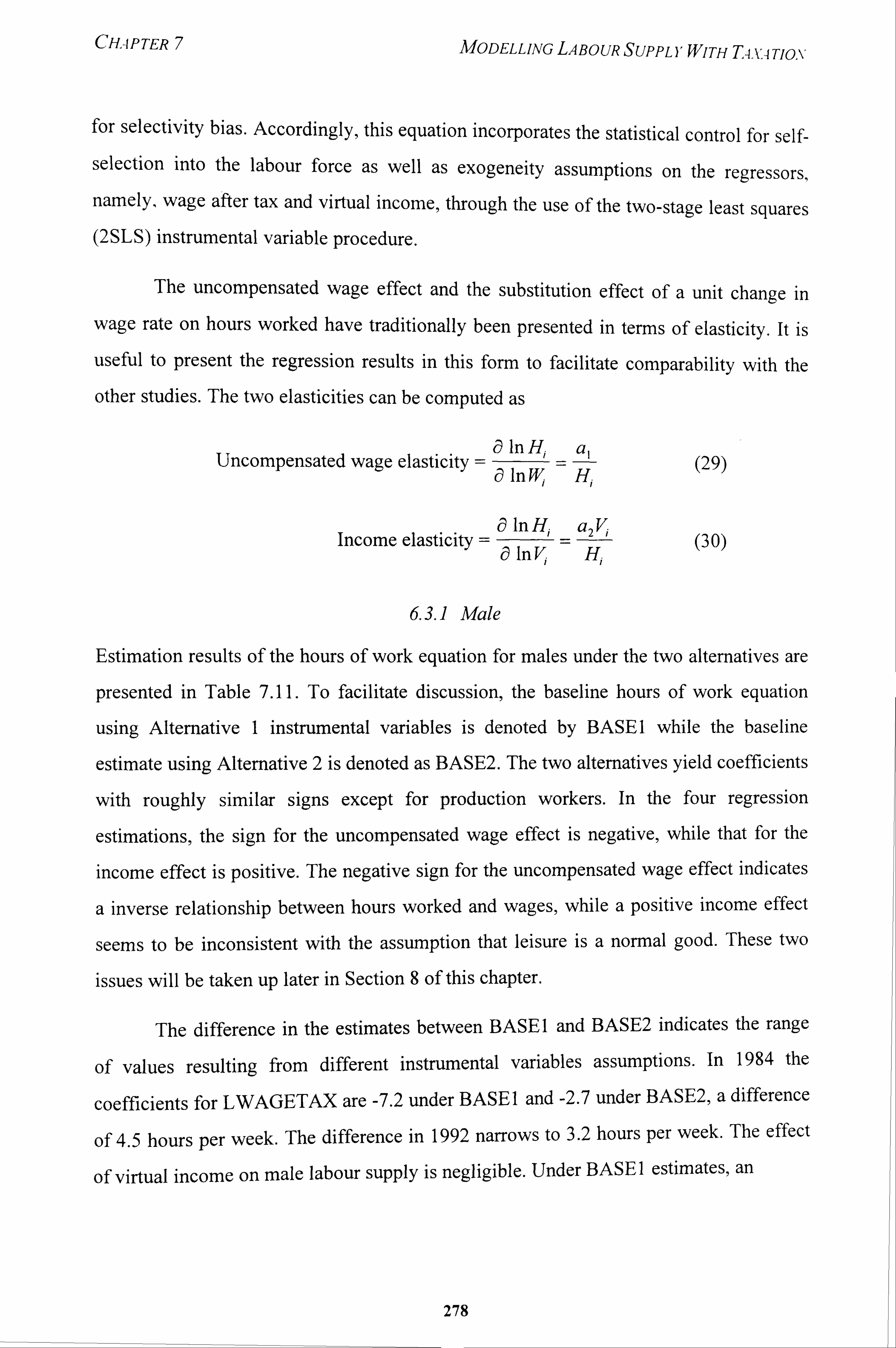
CHAPTER 7 MODELLING LABOUR SUPPLYWITH TAxA Tio, \,

for selectivity bias. Accordingly, this equation incorporates the statistical control for self- selection into the labour force as well as exogeneity assumptions on the regressors,

namely, wage after tax and virtual income, through the use of the two-stage least squares (2SLS) instrumental variable procedure.

The uncompensated wage effect and the substitution effect of a unit change in

wage rate on hours worked have traditionally been presented in terms of elasticity. It is

useful to present the regression results in this form to facilitate comparability with the

other studies. The two elasticities can be computed as

Uncompensated wage elasticity =a In H,

- a, (29)

0 InWi Hi

c9 In Hi aV Income elasticity =-2i (30) a InV, H,

6.3.1 Male

Estimation results of the hours of work equation for males under the two alternatives are

presented in Table 7.11. To facilitate discussion, the baseline hours of work equation

using Alternative I instrumental variables is denoted by BASE1 while the baseline

estimate using Alternative 2 is denoted as BASE2. The two alternatives yield coefficients

with roughly similar signs except for production workers. In the four regression

estimations, the sign for the uncompensated wage effect is negative, while that for the

income effect is positive. The negative sign for the uncompensated wage effect indicates

a inverse relationship between hours worked and wages, while a positive income effect

seems to be inconsistent with the assumption that leisure is a normal good. These two

issues will be taken up later in Section 8 of this chapter.

The difference in the estimates between BASEI and BASE2 indicates the range

of values resulting from different instrumental variables assumptions. In 1984 the

coefficients for LWAGETAX are -7.2 under BASE I and -2.7 under BASE2, a difference

of 4.5 hours per week. The difference in 1992 narrows to 3.2 hours per week. The effect

of virtual income on male labour supply is negligible. Under BASE I estimates, an

278

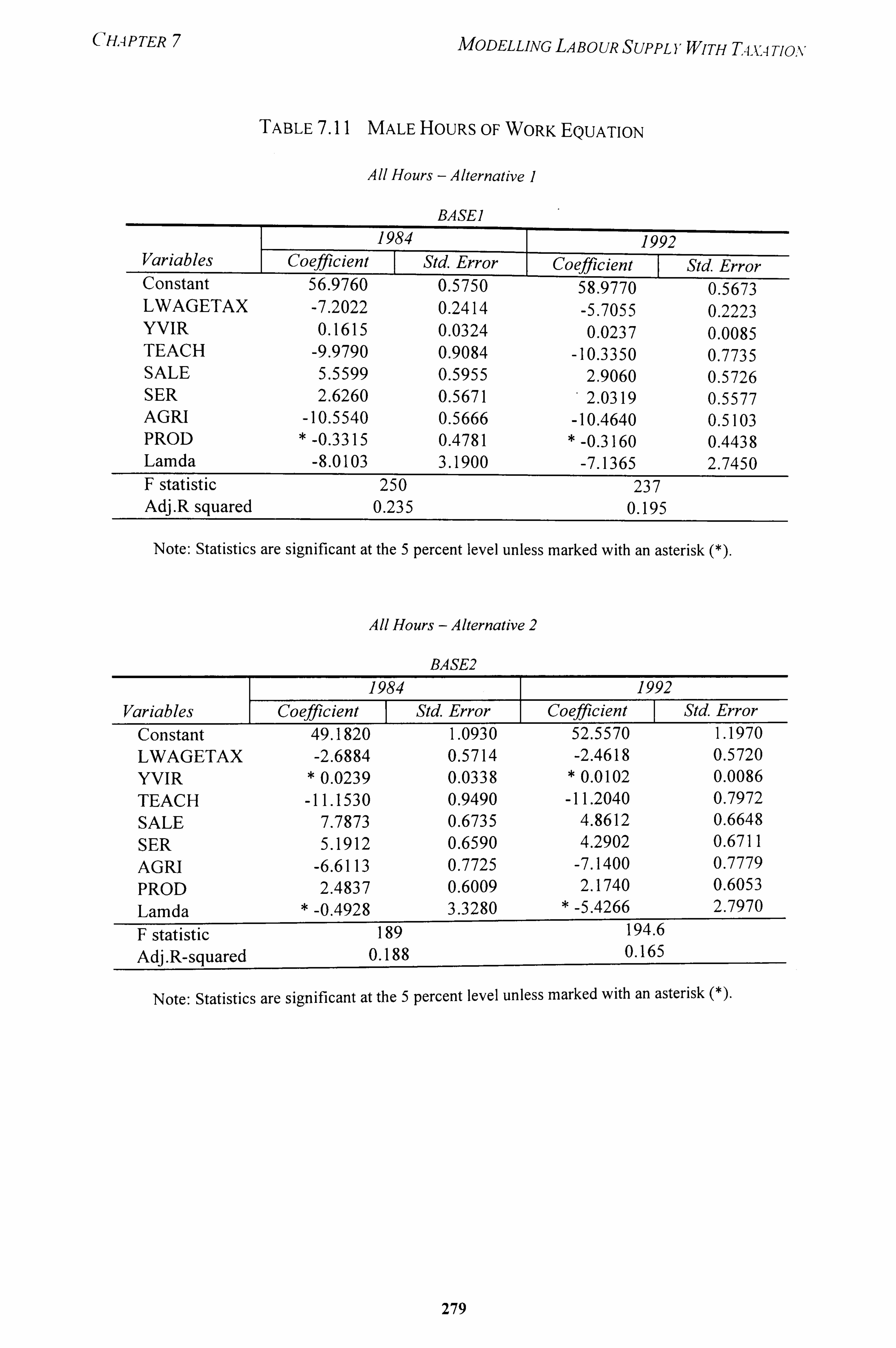
HAPTER MODELLjNG LABOUR SUPPLYWITH TIV4 TION

TABLE 7.11 MALE HOURS OF WORK EQUATION

All Hours - Alternative I

Variables Constant LWAGETAX YVIR TEACH SALE SER AGRI PROD Lamda F statistic Adj. R squared

BASE]

1984 1992 Coefficient Std. Error Coefficient Std Error

56.9760 0.5750 58.9770 0.5673 -7.2022 0.2414 -5.7055 0.2223 0.1615 0.0324 0.0237 0.0085

-9.9790 0.9084 -10.3350 0.7735 5.5599 0.5955 2.9060 0.5726 2.6260 0.5671 2.0319 0.5577

-10.5540 0.5666 -10.4640 0.5103 -0.3315 0.4781 -0.3160 0.4438 -8.0103 3.1900 -7.1365 2.7450

250 237 0.235 0.195


All Hours - Alternative 2

BASE2

1984 1992 Variables Coefficient Std. Error Coefficient Std. Error

Constant 49.1820 1.0930 52.5570 1.1970 LWAGETAX -2.6884 0.5714 -2.4618 0.5720 YVIR 0.0239 0.0338 0.0102 0.0086 TEACH -11.1530 0.9490 -11.2040 0.7972 SALE 7.7873 0.6735 4.8612 0.6648 SER 5.1912 0.6590 4.2902 0.6711 AGRI -6.6113 0.7725 -7.1400 0.7779 PROD 2.4837 0.6009 2.1740 0.6053 Lamda -0.4928 3.3280 -5.4266 2.7970

F statistic 189 194.6 Adj. R-squared 0.188 0.165


279

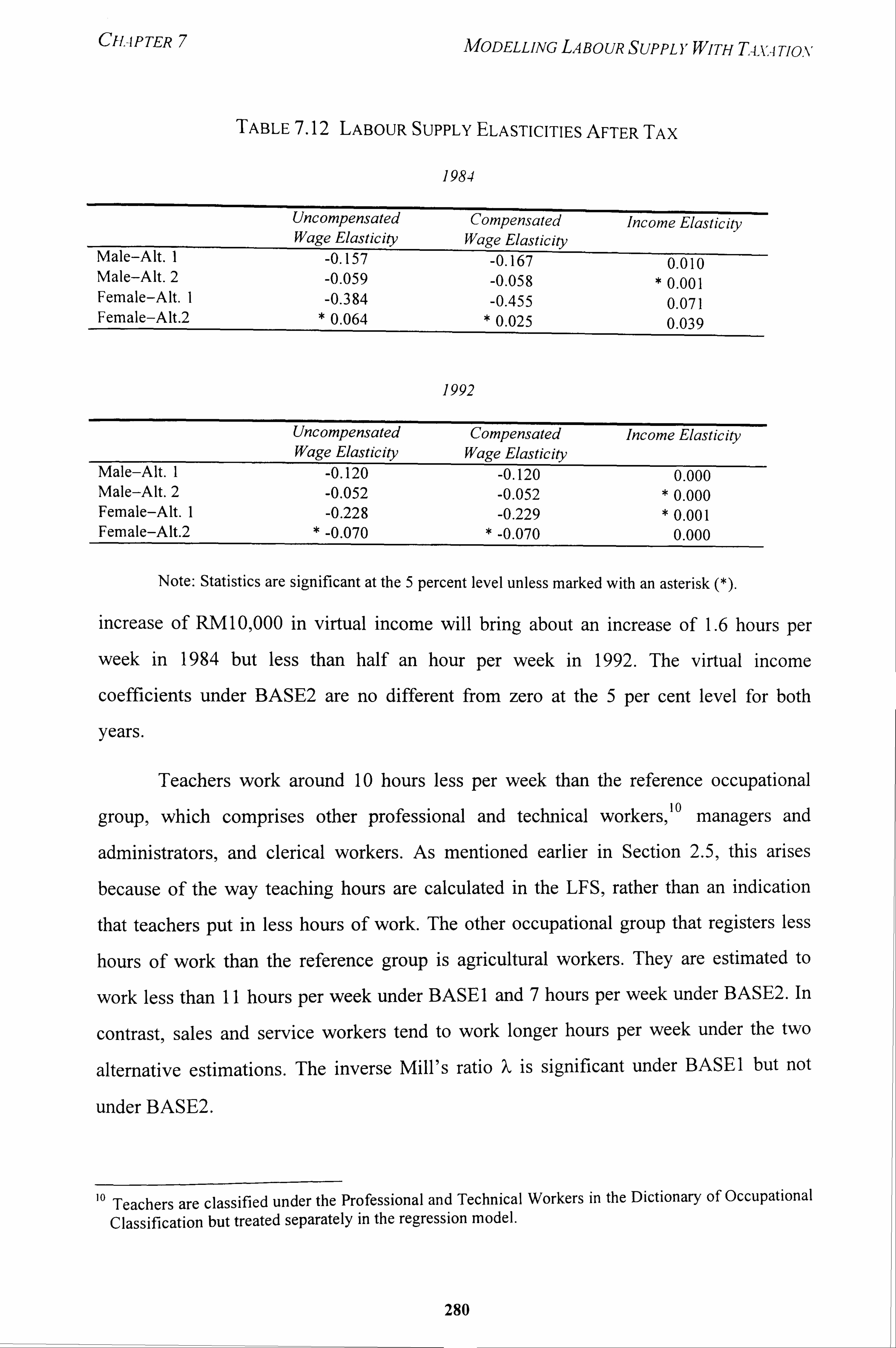
Cii. -iPTER 7 MODELLiNG LABOUR SUPPLYWITH T4-, k,. 4 Tim,

TABLE 7.12 LABOUR SUPPLY ELASTICITIEs AFTER TAX

1984

Uncompensated Wage Elasticity

Compensated Wage Elasticity

Income Elasticity

Male-Alt. 1 -0.157 -0.167 0.010 Male-Alt. 2 -0.059 -0.058 0.001 Female-Alt. 1 -0.384 -0.455 0.071 Female-Alt. 2 0.064 0.025 0.039

1992

Uncompensated Compensated Income Elasticity Wage Elasticity Wage Elasticity

Male-Alt. 1 -0.120 -0.120 0.000 Male-Alt. 2 -0.052 -0.052 * 0.000 Female-Alt. 1 -0.228 -0.229 * 0.001 Female-Alt. 2 -0.070 -0.070 0.000


increase of RM10,000 in virtual income will bring about an increase of 1.6 hours per

week in 1984 but less than half an hour per week in 1992. The virtual income

coefficients under BASE2 are no different from zero at the 5 per cent level for both

years.

Teachers work around 10 hours less per week than the reference occupational

group, which comprises other professional and technical workers, 10 managers and

administrators, and clerical workers. As mentioned earlier in Section 2.5, this arises

because of the way teaching hours are calculated in the LFS, rather than an indication

that teachers put in less hours of work. The other occupational group that registers less

hours of work than the reference group is agricultural workers. They are estimated to

work less than II hours Per week under BASE1 and 7 hours per week under BASE2. In

contrast, sales and service workers tend to work longer hours per week under the two

alternative estimations. The inverse Mill's ratio ?, is significant under BASEI but not

under BASE2.

10 Teachers are classified under the Professional and Technical Workers in the Dictionary of Occupational

Classification but treated separately in the regression model.

280

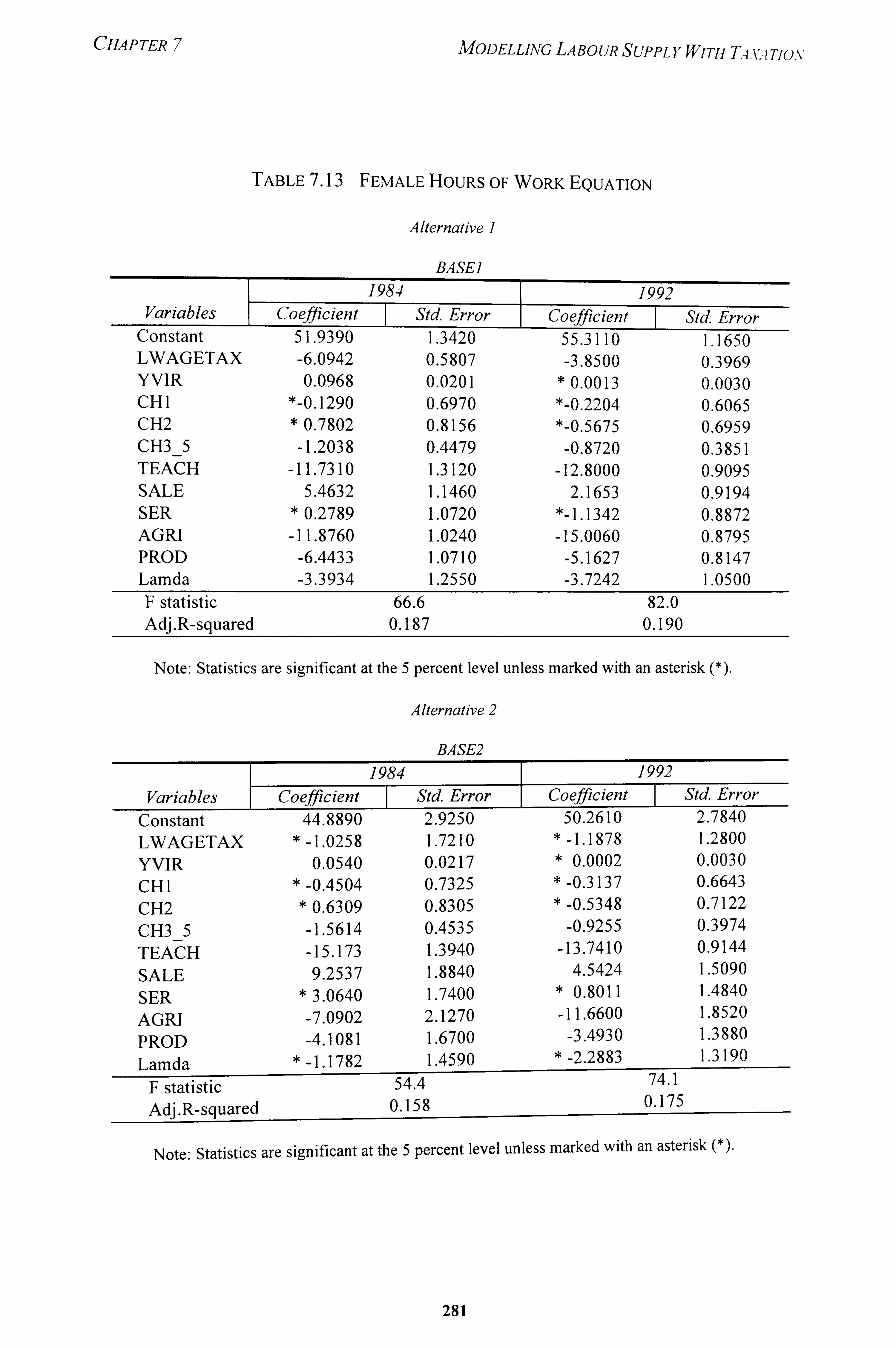
CHAPTER MODELLiNG LABOUR SUPPLYWITH TAx-i Tio. v

TABLE 7.13 FEMALE HOURS OF WORK EQUATION

A Iternative I

BASE]

1984 -

1992 Variables Coefficient Std. Error Coefficient Std. Error

Constant 51.9390 1.3420 55.3110 1.1650 LWAGETAX -6.0942 0.5807 -3.8500 0.3969 YVIR 0.0968 0.0201 0.0013 0.0030 CHI *-0.1290 0.6970 *-0.2204 0.6065 CH2 0.7802 0.8156 *-0.5675 0.6959 CH3_5 -1.2038 0.4479 -0.8720 0.3851 TEACH -11.7310 1.3120 -12.8000 0.9095 SALE 5.4632 1.1460 2.1653 0.9194 SER 0.2789 1.0720 1.1342 0.8872 AGRI -11.8760 1.0240 -15.0060 0.8795 PROD -6.4433 1.0710 -5.1627 0.8147 Lamda -3.3934 1.2550 -3.7242 1.0500 F statistic 66.6 82.0 Adj. R-squared 0.187 0.190


Alternative 2

BASE2

Constant 44.8890 2.9250 50.2610 2.7840 LWAGETAX * -1.0258 1.7210 * -1.1878 1.2800 YVIR 0.0540 0.0217 * 0.0002 0.0030 CHI * -0.4504 0.7325 * -0.3137 0.6643 CH2 0.6309 0.8305 * -0.5348 0.7122 CH3 5 -1.5614 0.4535 -0.9255 0.3974

TEACH -15.173 1.3940 -13.7410 0.9144

SALE 9.2537 1.8840 4.5424 1.5090

SER 3.0640 1.7400 0.8011 1.4840

AGRI -7.0902 2.1270 -11.6600 1.8520

PROD -4.1081 1.6700 -3.4930 1.3880

Lamda -1.1782 1.4590 -2.2883 1.3190

F statistic 54.4 74.1

Adj. R-squared 0.158 0.175


281

H, 4PTER MODELLiNG LABOUR SUPPL YWITH T4, u Tio. v

As shown in Table 7.12, the uncompensated wage elasticities are low under both

alternatives. They are -0.157 in 1984 and -0-120 in 1992 under BASEL When socio- demographic variables are used as instruments for. net wage for BASE2, the uncompensated wage elasticities become even more inelastic at around -0.05. The income elasticities are very small or zero under both alternatives.

6.3.2 Female

Table 7.13 shows the hours of work estimations under the two alternatives. The F

statistics and adjusted R-squared for 1984 and 1992 are generally similar under the two

alternative assumptions. The coefficients for LWAGETAX are significant under BASE1

but not under BASE2. In the case of virtual income,, the estimated coefficients are

significant but very small for 1984. The change in virtual income has to be very large for

there to be some effect on female labour supply. For instance, the virtual income in 1984

has to change by RM100,000 before registering a change of 10 hours per week for the

females under ALTI and 5 hours per week under ALT2. In 1992 the change in female

labour supply arising from a change in virtual income will not be significantly different

from zero for both alternatives.

It appears that while the presence of young children reduces the likelihood of

female participation, they do not affect the working hours of mothers who choose to

work. However, the coefficients are statistically insignificant and children between the

ages of 3 to 5 years would only reduce the working hours of their mothers by one to one

and a half hours per week. There appears to be a strong link between occupational groups

and hours of work. Females in the teaching, agricultural, and production occupations

generally work shorter hours per week than the reference occupational group, while

females in the sales and service occupations work longer hours. The difference in hours

of work between the two alternatives and for both the years can be substantial for

teachers (12-15 hours), agricultural workers (7-15 hours), sales workers (2-9 hours), and

production workers (3-6 hours).

In terms of the elasticity estimates, the uncompensated wage elasticities for

females under BASEI are -0.384 for 1984 and -0.228 for 1992, about twice as large as

282

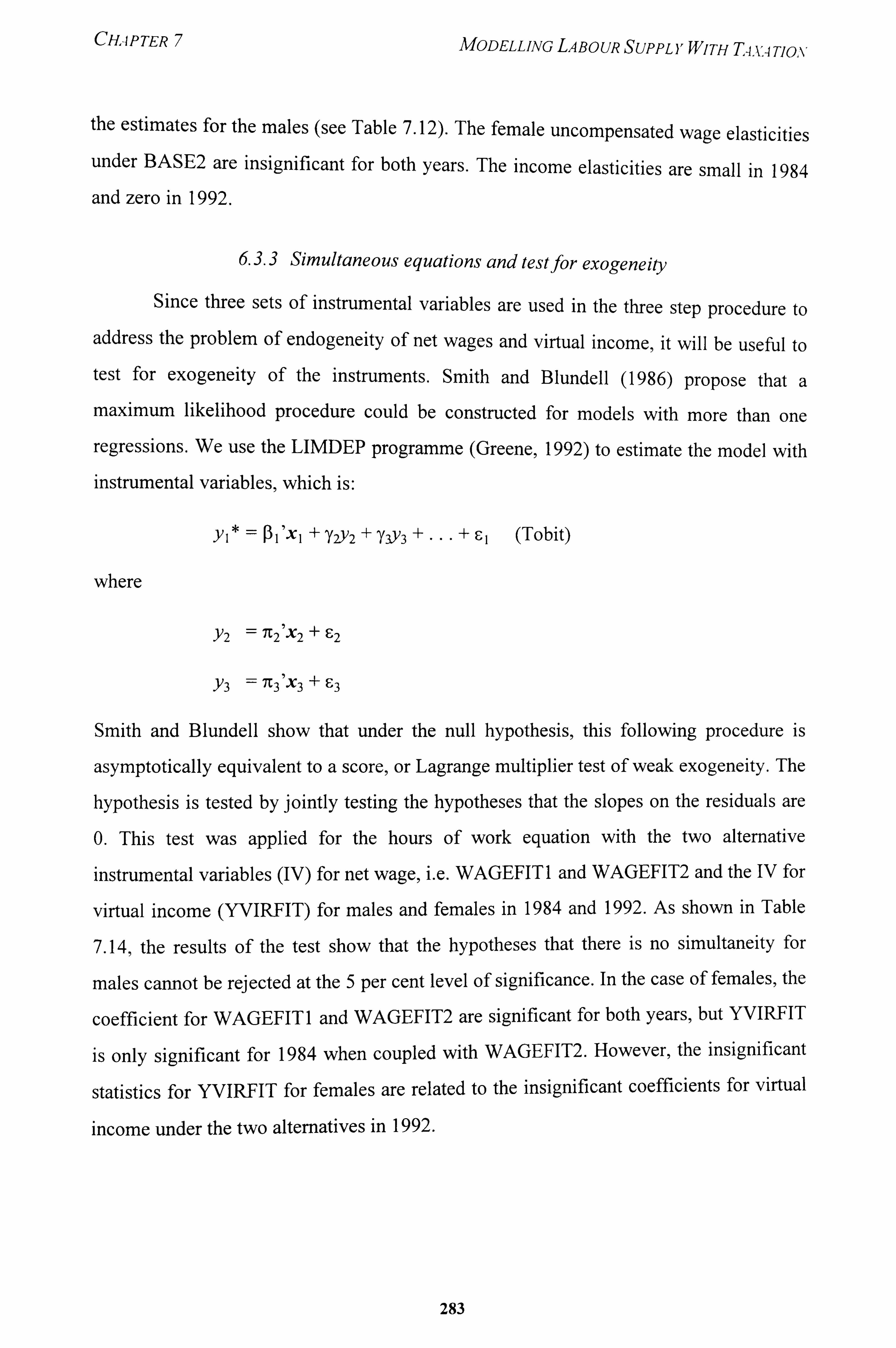
CHAPTER 7 MODELLING LABOUR SUPPLYWITH T-i. V. 4 TION

the estimates for the males (see Table 7.12). The female uncompensated wage elasticities under BASE2 are insignificant for both years. The income elasticities are small in 1984 and zero in 1992.

6.3.3 Simultaneous equations and testfor exogeneiry

Since three sets of instrumental variables are used in the three step procedure to

address the problem of endogeneity of net wages and virtual income, it will be useful to test for exogeneity of the instruments. Smith and Blundell (1986) propose that a maximum likelihood procedure could be constructed for models with more than one

regressions. We use the LIMDEP programme (Greene, 1992) to estimate the model with instrumental variables, which is:

Yl * '-:: ßl'XI + 72Y2 + 71Y3 +---+ F-1 (Tobit)

where

Y2 ý 7C2'X2 + 62

Y3 : --: 7C3 X3 + F13

Smith and Blundell show that under the null hypothesis, this following procedure is

asymptotically equivalent to a score, or Lagrange multiplier test of weak exogeneity. The

hypothesis is tested by jointly testing the hypotheses that the slopes on the residuals are

0. This test was applied for the hours of work equation with the two alternative

instrumental variables (IV) for net wage, i. e. WAGEFITI and WAGEFIT2 and the IV for

virtual income (YVIRFIT) for males and females in 1984 and 1992. As shown in Table

7.14, the results of the test show that the hypotheses that there is no simultaneity for

males cannot be rejected at the 5 per cent level of significance. In the case of females, the

coefficient for WAGEFITI and WAGEFIT2 are significant for both years, but YVIRFIT

is only significant for 1984 when coupled with WAGEFIT2. However, the insignificant

statistics for YVIRFIT for females are related to the insignificant coefficients for virtual

income under the two alternatives in 1992.

283

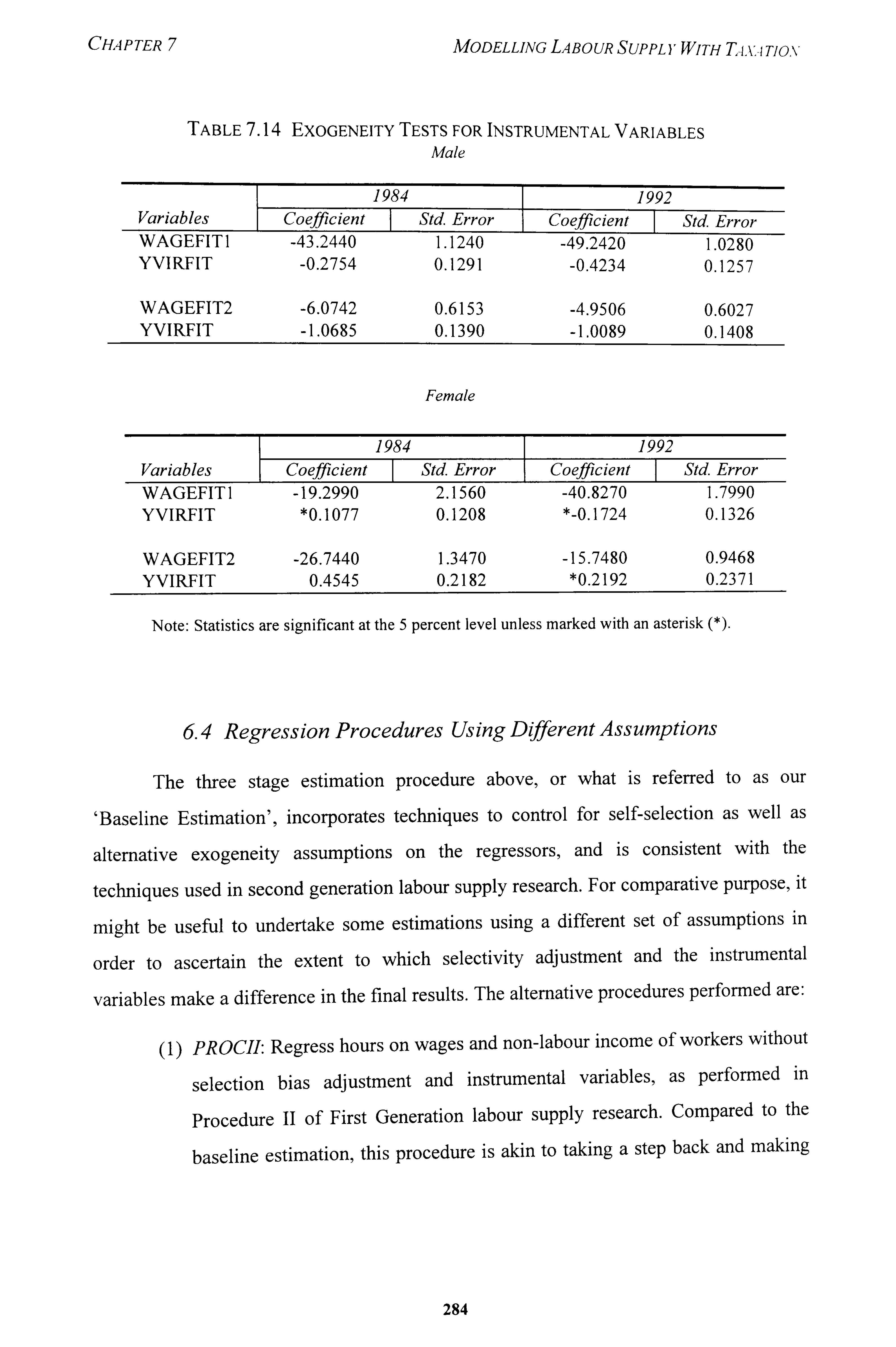
CH. 4P TER MODELLING LABOUR SUPPLYWITH Tix-i Tiav

TABLE 7.14 EXOGENEITY TESTS FOR INSTRUMENTAL VARIABLES Male

WAGEFIT2 YVIRFIT

-6.0742 0.6153

-1.0685 0.1390

'11IJ P. rrr)r

-4.9506 0.6027

-1.0089 0.1408

Female

. -ii" r. rrt)r

WAGEFIT2 -26.7440 1.3470 -15.7480 0.9468 YVIRFIT 0.4545 0.2182 *0.2192 0.2371


6.4 Regression Procedures Using Different Assumptions

The three stage estimation procedure above, or what is referred to as our

'Baseline Estimation', incorporates techniques to control for self-selection as well as

alternative exogeneity assumptions on the regressors, and is consistent with the

techniques used in second generation labour supply research. For comparative purpose, it

might be useful to undertake some estimations using a different set of assumptions in

order to ascertain the extent to which selectivity adjustment and the instrumental

variables make a difference in the final results. The alternative procedures performed are:

(1) PROCIL Regress hours on wages and non-labour income of workers without

selection bias adjustment and instrumental variables, as performed in

Procedure 11 of First Generation labour supply research. Compared to the

baseline estimation, this procedure is akin to taking a step back and making

284

WAGEFITI -43.2440 1.1240 -49.2420 1.0280 YVIRFIT -0.2754 0.1291 -0.4234 0.1257

WAGEFITI -19.2990 2.1560 -40.8270 1.7990 YVIRFIT *0.1077 0.1208 *-0.1724 0.1326

CHAPTER 7 MODELLiNG LABOUR SUPPL YWITH TA-u Tio, v

the estimations without addressing the selection bias and endogeneity problems.

(2) PROCIISA: Regress hours on wages and non-labour income of workers with selectivity adjustments but without use of instrumental variables. As discussed in Chapter 4, the critique against Procedure 11 is that it suffers from selection bias as well as endogeneity. Accordingly, we perform the

same regression but this time addressing the selection bias. The difference between the results of this alternative and the baseline estimates can be

attributed to the problems of endogeneity and measurement.

(3) RESHRI and RESHR2: Estimating the hours of work equation for those

working between 25-60 hours with selectivity adjustment and adopting the

two alternative instrumental variables procedures. The three-stage baseline

estimation of labour supply equation parameters is performed for all

reported working hours. Measurement errors in hours of work are

transmitted to wage measurement. When a respondent reports long working

hours for the week, either as a result of overtime work or the difficulty of

estimating the number of hours worked for some occupations, this will

result in lower estimated wage rate. On the other hand, if a respondent

reports short working hours for the week, say in the case of bad weather or

slack period for a contract worker, this will cause an upward bias in the

estimated wage rate. Errors in reporting hours worked for the week are

inevitably transmitted to the estimated wage rate, causing a spurious

negative relationship between the hours worked and wage rate. This

alternative estimation procedure removes from the sample those who report

in working hours at the two ends of the hours spectrum which are more

likely to be affected by misreporting. By limiting the analysis to those

working between 25-60 hours per week, the sample covers the majority of

the workers in regular jobs, namely, around 95 per cent of the working

285

CH-4PTER 7 MODELLING LABOUR SUPPLYWITH TA-v-1 TION

males and 70 per cent of the working fernales. ' 1 The lower limit is set at 25 hours rather than 30 hours so as not to exclude teachers from the sample.

(4) PRETXSA and PRETXSAIV: Estimating pre-tax hours of work equation with

selectivity adjustment. In the earlier sections, we estimate the labour supply

equation parameters after controlling for taxes and using after-tax marginal

wage rate and virtual income in the regression equations. We now take a step back by examining how the labour supply function changes before taxes are

taken into account. In fact,, the bulk of the studies which estimate the

parameters of the labour supply function do so without considering taxation.

Comparison of the two sets of estimated parameters show the importance of

taxes in influencing labour supply. The estimations are performed using two

alternative procedures. The first alternative uses the probit estimation

procedure to yield the participation equation parameters and derive the

inverse Mill's ratio, which is then used to estimate the hours of work

equation. This alternative may be affected by the endogeneity of wages to

hours worked, but it is useftil for comparative purpose since it generates

results which are somewhat parallel to those obtained from Procedure 11 with

selection adjustment. In the second alternative, the three step procedure was

performed, using the socio-demographic variables as instruments for gross

wage.

(5) PRETXSAIV and RPRETXSAIV. - The first procedure, PRETXSAIV,

estimates pre-tax hours of work equation with selectivity adjustment and

instrumental variables. This regression follows the three step procedure used

in the baseline estimation procedure. The purpose of instrumenting for net

wage is to address the endogeneity problem as well as remove the spurious

II For example, in 1984 about 6 per cent of the males reported working less than 26 hours, while another

10 per cent worked over 60 hours. The equivalent proportion of women working these hours are 18 per

cent and 9 per cent, respectively. The frequency of respondents working less than 25 hours per week are

highest among farmers, sales workers, transport equipment operators, waitress and cleaners, and

building trades. Respondents who work more than 60 hours per week tend to be working proprietors,

drivers, vendors, sales and shop assistants, cooks, maids and personal services workers, fishermen and

farmers (see Table 7.26).

286

CHAPTER 7 MODELLiNG LABOUR SUPPLYWITH T4x, 4 Tim,

negative re ation between Hi and Wi should there be a random measurement error in Hi. The variables used to instrument for pre-tax wage are identical to those Alternative 11 of the baseline estimation. RPRETXSAIV follows the same estimation procedure as PRETXSAIV but is applied to the restricted sample of those working between 25-60 hours.

6.4.1 Procedure H with and without selectivity adjustments

The regression results for males and females using Procedure 11 (PROCII)

correspond fairly closely to the three step procedure of the baseline estimations (see

Table 7.15 and Table 7.16). The signs are in the same direction, although the coefficients for net wage and virtual income for both years and sexes are slightly lower than BASEI

estimates but higher than BASE2 estimates. The elasticity estimates for both sexes are

given in Table 7.17 and Table 7.18. The PROCII elasticities have the same signs as the

baseline elasticities. The value of the elasticity estimates of Procedure 11 fall between the

values of the two alternatives of the baseline estimates. In 1984 the male elasticities for

the uncompensated wage effect under PROCII is -0.139, compared with -0.157 under

BASEI and -0.059 under BASE2. The PROCII elasticity estimates for females are,

however, closer to the elasticities obtained under BASEll than BASEL The income

elasticities are very small and not significantly different from zero at the 5 per cent level.

Since the compensated wage elasticity is calculated as a residual, where the income

elasticity is close to zero the compensated wage elasticity will be very close to the value

of the uncompensated wage elasticity.

The next set of regressions are performed using Procedure II with selectivity

adjustment (PROCIISA). The difference in estimates obtained from PROCII and

PROCIISA can be attributed to the effect of selection bias. The inclusion of the

selectivity adjustment has the effect of increasing the absolute value of the LWAGETAX

coefficient, with the estimates for females showing much greater difference than the

males. Given the very high male participation of 97.5 per cent compared with barely 40

per cent for females, the correction for self-selection is considerably more important for

the females than the males.

287

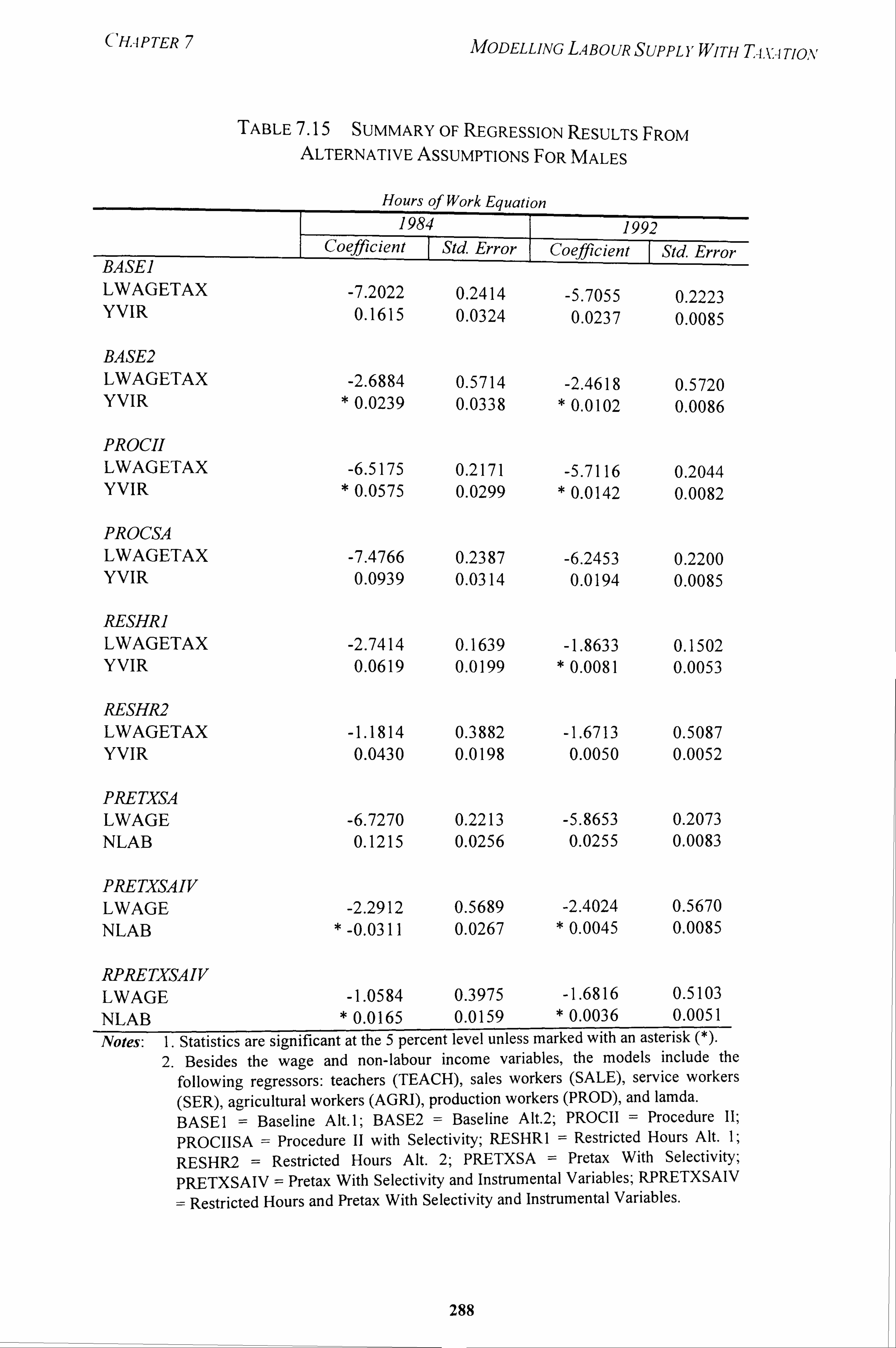
HAPTER 7 MODELLING LABOUR SUPPLYWITH T4x-i Tim,

TABLE 7.15 SUMMARY OF REGRESSION RESULTS FROM ALTERNATIVE ASSUMPTIONS FOR MALES

Hours of Work Equation 1984 1992

Coefficient ý -Std Error Coefficient Std Error BASE] LWAGETAX -7.2022 0.2414 -5.7055 0.2223 YVIR 0.1615 0.0324 0.0237 0.0085

BASE2 LWAGETAX -2.6884 0.5714 -2.4618 0.5720 YVIR * 0.0239 0.0338 * 0.0102 0.0086

PROM LWAGETAX -6.5175 0.2171 -5.7116 0.2044 YVIR * 0.0575 0.0299 * 0.0142 0.0082

PROM LWAGETAX -7.4766 0.2387 -6.2453 0.2200 YVIR 0.0939 0.0314 0.0194 0.0085

RESHRI LWAGETAX -2.7414 0.1639 -1.8633 0.1502 YVIR 0.0619 0.0199 0.0081 0.0053

RESHR2 LWAGETAX -1.1814 0.3882 -1.6713 0.5087 YVIR 0.0430 0.0198 0.0050 0.0052

PRETXSA LWAGE -6.7270 0.2213 -5.8653 0.2073 NLAB 0.1215 0.0256 0.0255 0.0083

PREMAN LWAGE -2.2912 0.5689 -2.4024 0.5670 NLAB -0.0311 0.0267 * 0.0045 0.0085

RPRETXSAIV LWAGE -1.0584 0.3975 -1.6816 0.5103 NLAB 0.0165 0.0159 * 0.0036 0.0051 Notes: 1. Statistics are significant at the 5 percent level unless marked with an asterisk (*).

2. Besides the wage and non-labour income variables, the models include the following regressors: teachers (TEACH), sales workers (SALE), serv ice workers (SER), agricultural workers (AGRI), p roduction workers (PROD), and l amda. BASEI = Baseline Alt. 1; BASE2 = Baseline Alt. 2; PROCII = Procedure 11; PROCIISA = Procedure 11 with Selectivity; RESHRI = Restricted H ours Alt. 1; RESHR2 = Restricted Hours Alt. 2; PRETXSA = Pretax With Selectivity; PRETXSAIV = Pretax With Selectivit y and Instrumental Variables; RP RETXSAIV

= Restricted Hours and Pretax With Selectivity and Instrumental Variab les.

288

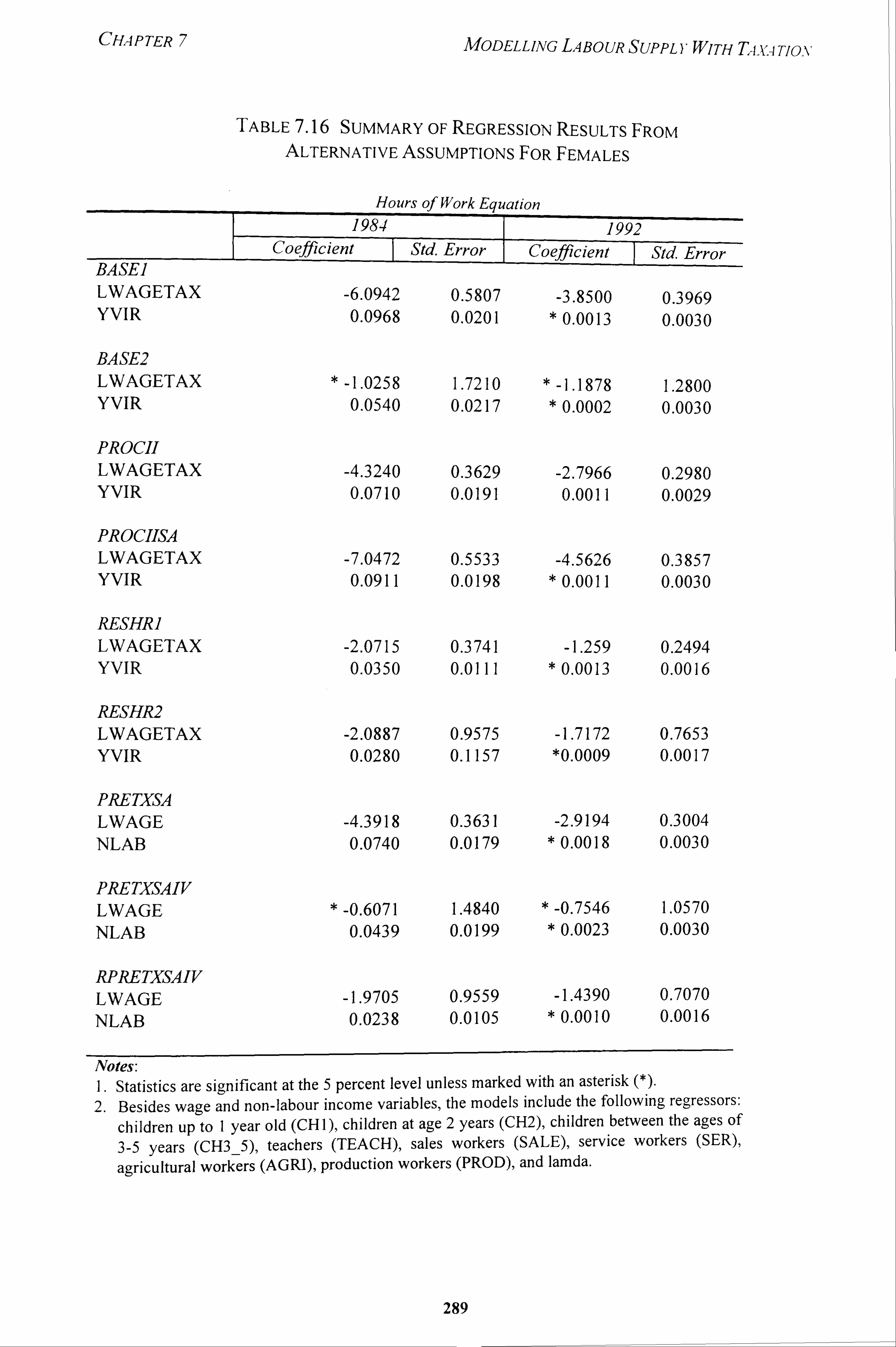
CHA P TER 7 MODELLiNG LABOUR SUPPLYWITH T-i-u Tim,

TABLE 7.16 SUMMARY OF REGRESSION RESULTS FROM ALTERNATIVE ASSUMPTIONS FOR FEMALES

Hours of Work Equation 1984 1992

Coefficient T -Std. Error Coefficient- I Std. Error BASE] LWAGETAX -6.0942 0.5807 -3.8500 0.3969 YVIR 0.0968 0.0201 0.0013 0.0030

BASE2 LWAGETAX -1.0258 1.7210 -1-1878 1.2800 YVIR 0.0540 0.0217 0.0002 0.0030

PROCII LWAGETAX -4.3240 0.3629 -2.7966 0.2980 YVIR 0.0710 0.0191 0.0011 0.0029

PROCIISA LWAGETAX -7.0472 0.5533 -4.5626 0.3857 YVIR 0.0911 0.0198 0.0011 0.0030

RESHRI LWAGETAX -2.0715 0.3741 -1.259 0.2494 YVIR 0.0350 0.0111 0.0013 0.0016

RESHR2 LWAGETAX -2.0887 0.9575 -1.7172 0.7653 YVIR 0.0280 0.1157 *0.0009 0.0017

PRETXSA LWAGE -4.3918 0.3631 -2.9194 0.3004 NLAB 0.0740 0.0179 0.0018 0.0030

PRETXSAIV LWAGE -0.6071 1.4840 -0.7546 1.0570 NLAB 0.0439 0.0199 0.0023 0.0030

RPRETXSAIV LWAGE -1.9705 0.9559 -1.4390 0.7070 NLAB 0.0238 0.0105 0.0010 0.0016

Notes: 1. Statistics are significant at the 5 percent level unless marked with an asterisk 2. Besides wage and non-labour income variables, the models include the following regressors:

children up to I year old (CHI), children at age 2 years (CH2), children between the ages of

3-5 years (CH3_5), teachers (TEACH), sales workers (SALE), service workers (SER),

agricultural workers (AGRI), production workers (PROD), and lamda.

289

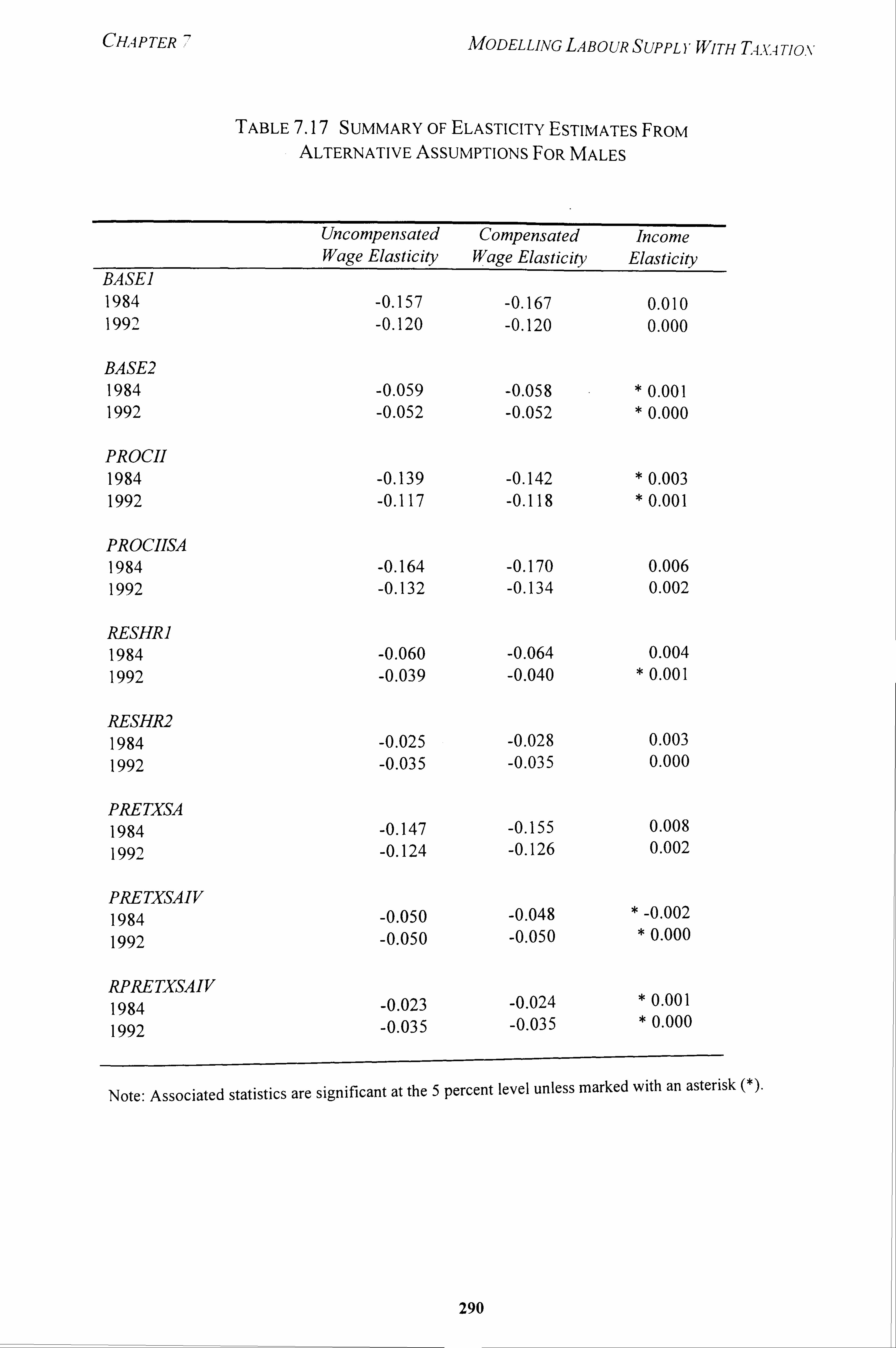
CHA P TER , MODELLiNG LABOUR SUPPL)'WjTH TA-v. 4 Tio. v

TABLE 7.17 SUMMARY OF ELASTICITY ESTIMATES FROM ALTERNATIVE ASSUMPTIONS FOR MALES

Uncompensated Compensated Income Wage Elasticity Wage Elasticity Elasticity

BASE] 1984 -0.157 -0-167 0.010 199-1 -0.120 -0.120 0.000

BASE2 1984 -0.059 -0-058 * 0.001 1992 -0.052 -0.052 * 0.000

PROCII 1984 -0.139 -0.142 * 0.003 1992 -0.117 -0.118 * 0.001

PROCIISA 1984 -0.164 -0.170 0.006 1992 -0.132 -0.134 0.002

RESHRI 1984 -0.060 -0.064 0.004 1992 -0.039 -0.040 0.001

RESHR2 1984 -0.025 -0.028 0.003 1992 -0.035 -0.035 0.000

PRETXSA 1984 -0.147 -0.155 0.008

199') -0.124 -0.126 0.002

PRETXSAIV 1984 -0.050 -0.048 -0.002 1992 -0.050 -0.050 0.000

RPRETXSAIV 1984 -0.023 -0.024 * 0.001

1992 -0.035 -0.035 * 0.000

Note: Associated statistics are significant at the 5 percent level unless marked with an asterisk (*)

290

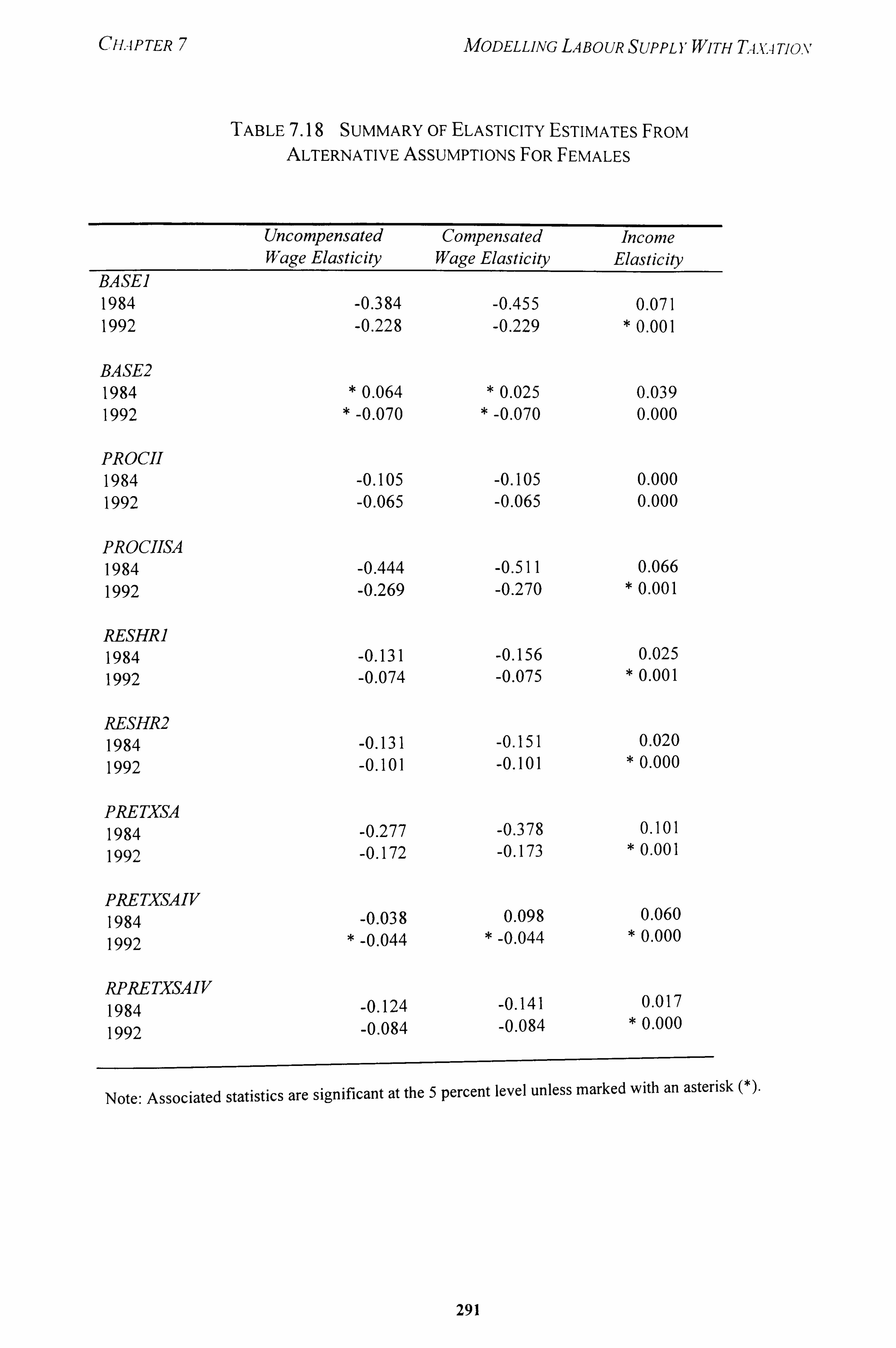
Cli. -iPTER 7 MODELLiNG LABOUR SUPPL YWJTH TAx. A Tjo. v

TABLE 7.18 SUMMARY OF ELASTICITY ESTIMATES FROM ALTERNATIVE ASSUMPTIONS FOR FEMALES

Uncompensated Compensated Income Wage Elasticity Wage Elasticity Elasticity

BASE] 1984 -0.384 -0.455 0.071 1992 -0.228 -0.229 0.001

BASE2 1984 0.064 0.025 0.039 1992 -0.070 -0.070 0.000

PROM 1984 -0.105 -0.105 0.000 1992 -0.065 -0.065 0.000

PROCIISA 1984 -0.444 -0.511 0.066 1992 -0.269 -0.270 0.001

RESHRI 1984 -0.131 -0.156 0.025 1992 -0.074 -0.075 0.001

RESHR2 1984 -0.131 -0.151 0.020 1992 -0.101 -0.101 0.000

PRETXSA 1984 -0.277 -0.378 0.101

1992 -0.172 -0.173 0.001

PRETXSAIV 1984 -0.038 0.098 0.060

1992 -0.044 -0.044 0.000

RPRETXSAIV 1984 -0.124 -0.141 0.017

1992 -0.084 -0.084 0.000

Note: Associated statistics are significant at the 5 percent level unless marked with an asterisk

91

CMPTER MODELLjNG LABOUR SUPPLYWITH TIV4 TION

The difference in the size of coefficients generated by PROCIISA and the baseline estimates provide an indication on the effect of the two alternative instrumental

NI'ariables on the estimates. The LWAGETAX coefficient estimates using instrumental

variable adjustment under Alternative I are fairly close to the PROCIISA estimates compared with those obtained from Alternative 2, which are much lower in absolute terms. This can be expected given the very high correlation between LWAGETAX and the instruments in Alternative I compared to a much lower correlation between LWAGETAX and the instruments in Alternative 2.

6.4.2 Restricting to 25-60 hours per week

In the estimation of the labour supply equation, restricting the sample of workers

to those working between 25-60 hours per week produces some interesting results. This

procedure was done to remove those who are underemployed or those for whom it is

difficult to estimate the hours worked because of the nature of their occupation or work

performed during the survey week. The issue of extreme values in the hours worked as

reported by the respondent is closely linked to the problem of hours misreporting which

causes a spurious negative relationship between hours and wages. Between the two

alternative instrumental variables used in the baseline estimations, Alternative 2 is

probably much better in getting around the problem of measurement error than

Alternative I which uses gross wage rate and gross wage rate squared as part of its

instruments. Although the argument behind Alternative I instrumental variables is that

the level of gross wage rate is quite independent of the hours worked by an individual

taxpayer, yet the gross wage rate is not completely free from the effects of measurement

error.

The labour supply equations with restricted hours are estimated after adjusting for

selectivity and applying the two alternative instrumental variables. Two features emerge

from the estimates. First, the difference in the coefficients between RESHRI and

RESHR2 is much smaller than those obtained from BASE1 and BASE2. Second, the

coefficient estimates for the restricted hours are much closer to BASE2 rather than

BASE1 estimates. In fact, one is tempted to say that the restricted hours estimates seem

292

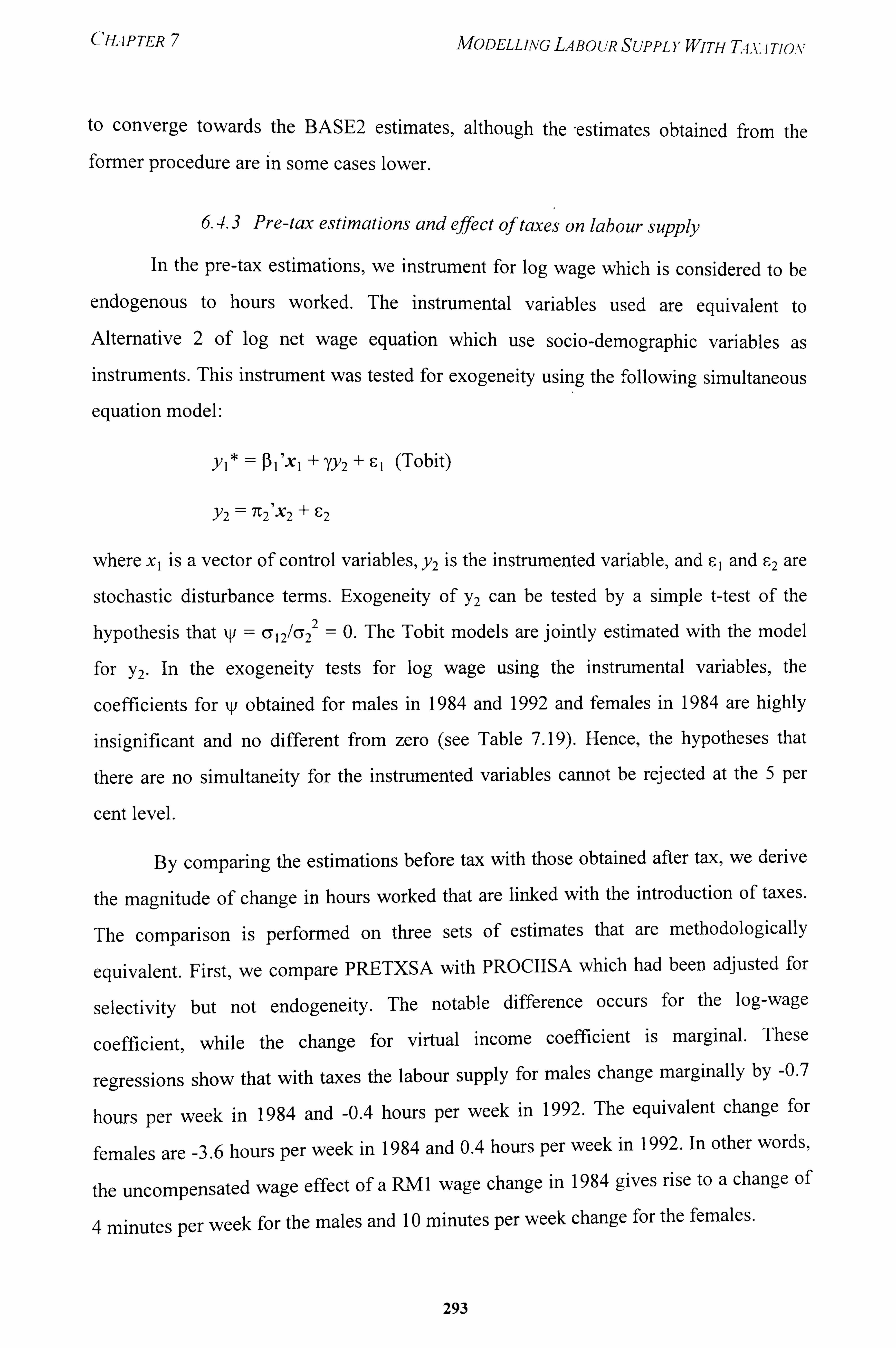
CH. 4PTER 7 MODELLING LABOUR SUPPLYWITH TAx, -i Tjo,, Nr

to converge towards the BASE2 estimates, although the -estimates obtained from the former procedure are in some cases lower.

6.4.3 Pre-tax estimations and effect of taxes on labour supply

In the pre-tax estimations, we instrument for log wage which is considered to be

endogenous to hours worked. The instrumental variables used are equivalent to

Alternative 2 of log net wage equation which use socio-demographic variables as instruments. This instrument was tested for exogeneity using the following simultaneous

equation model:

YI* "":::: P I'X I+ 7Y2 + F- 1 (Tobit)

Y2 : -": 7C2'X2 + F-2

where x, is a vector of control variables, Y2 is the instrumented variable, and E; I and E; 2are

stochastic disturbance terms. Exogeneity Of Y2 can be tested by a simple t-test of the 2 hypothesis thatV = CY I 21CY2 = 0. The Tobit models are jointly estimated with the model

for Y2- In the exogeneity tests for log wage using the instrumental variables, the

coefficients for V obtained for males in 1984 and 1992 and females in 1984 are highly

insignificant and no different from zero (see Table 7.19). Hence, the hypotheses that

there are no simultaneity for the instrumented variables cannot be rejected at the 5 per

cent level.

By comparing the estimations before tax with those obtained after tax, we derive

the magnitude of change in hours worked that are linked with the introduction of taxes.

The comparison is performed on three sets of estimates that are methodologically

equivalent. First, we compare PRETXSA with PROCIISA which had been adjusted for

selectivity but not endogeneity. The notable difference occurs for the log-wage

coefficient, while the change for virtual income coefficient is marginal. These

regressions show that with taxes the labour supply for males change marginally by -0.7

hours per week in 1984 and -0.4 hours per week in 1992. The equivalent change for

females are -3.6 hours per week in 1984 and 0.4 hours per week in 1992. In other words,

the uncompensated wage effect of a RMI wage change in 1984 gives rise to a change of

4 minutes per week for the males and 10 minutes per week change for the females.

293

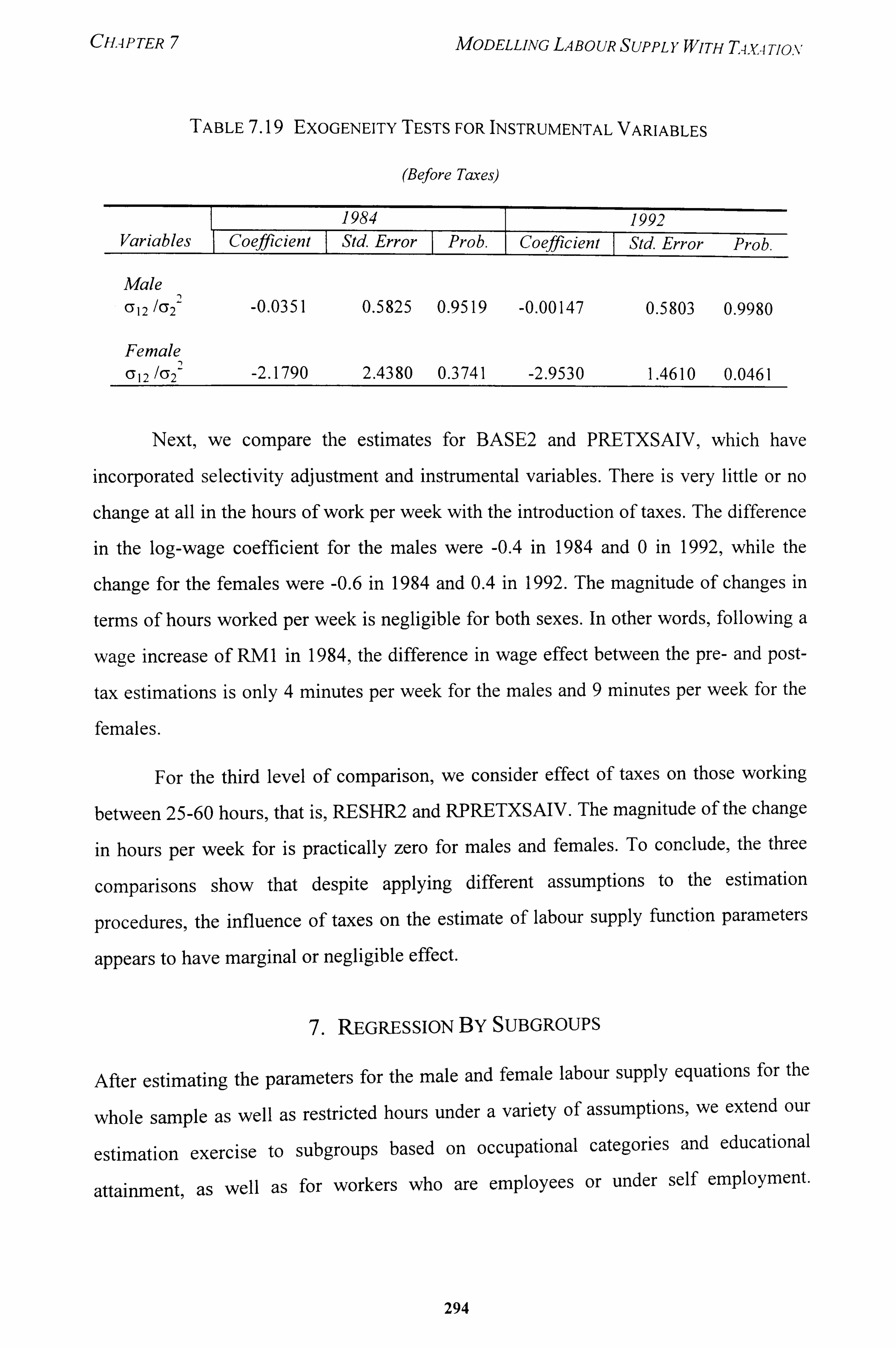
CH-4PTER MODELLiNG LABOUR SUPPLY WITH Tq. v4 Tiox

TABLE 7.19 EXOGENEITY TESTS FOR INSTRUMENTAL VARIABLES

(Before Taxes)

Male Cy 12 IC72 2

-0.0351 0.5825 0.9519 -0.00147 0.5803 0.9980

Female (3 12 1ý32 2

-2.1790 2.4380 0.3741 -2.9530 1.4610 0.0461

Next, we compare the estimates for BASE2 and PRETXSAIV, which have

incorporated selectivity adjustment and instrumental variables. There is very little or no

change at all in the hours of work per week with the introduction of taxes. The difference

in the log-wage coefficient for the males were -0.4 in 1984 and 0 in 1992, while the

change for the females were -0.6 in 1984 and 0.4 in 1992. The magnitude of changes in

terms of hours worked per week is negligible for both sexes. In other words, following a

wage increase of RMI in 1984, the difference in wage effect between the pre- and post-

tax estimations is only 4 minutes per week for the males and 9 minutes per week for the

females.

For the third level of comparison, we consider effect of taxes on those working

between 25-60 hours, that is, RESHR2 and RPRETXSAIV. The magnitude of the change

in hours per week for is practically zero for males and females. To conclude, the three

comparisons show that despite applying different assumptions to the estimation

procedures, the influence of taxes on the estimate of labour supply function parameters

appears to have marginal or negligible effect.

7. REGRESSiON BY SUBGROUPS

After estimating the parameters for the male and female labour supply equations for the

whole sample as well as restricted hours under a variety of assumptions, we extend our

estimation exercise to subgroups based on occupational categories and educational

attainment, as well as for workers who are employees or under self employment.

294

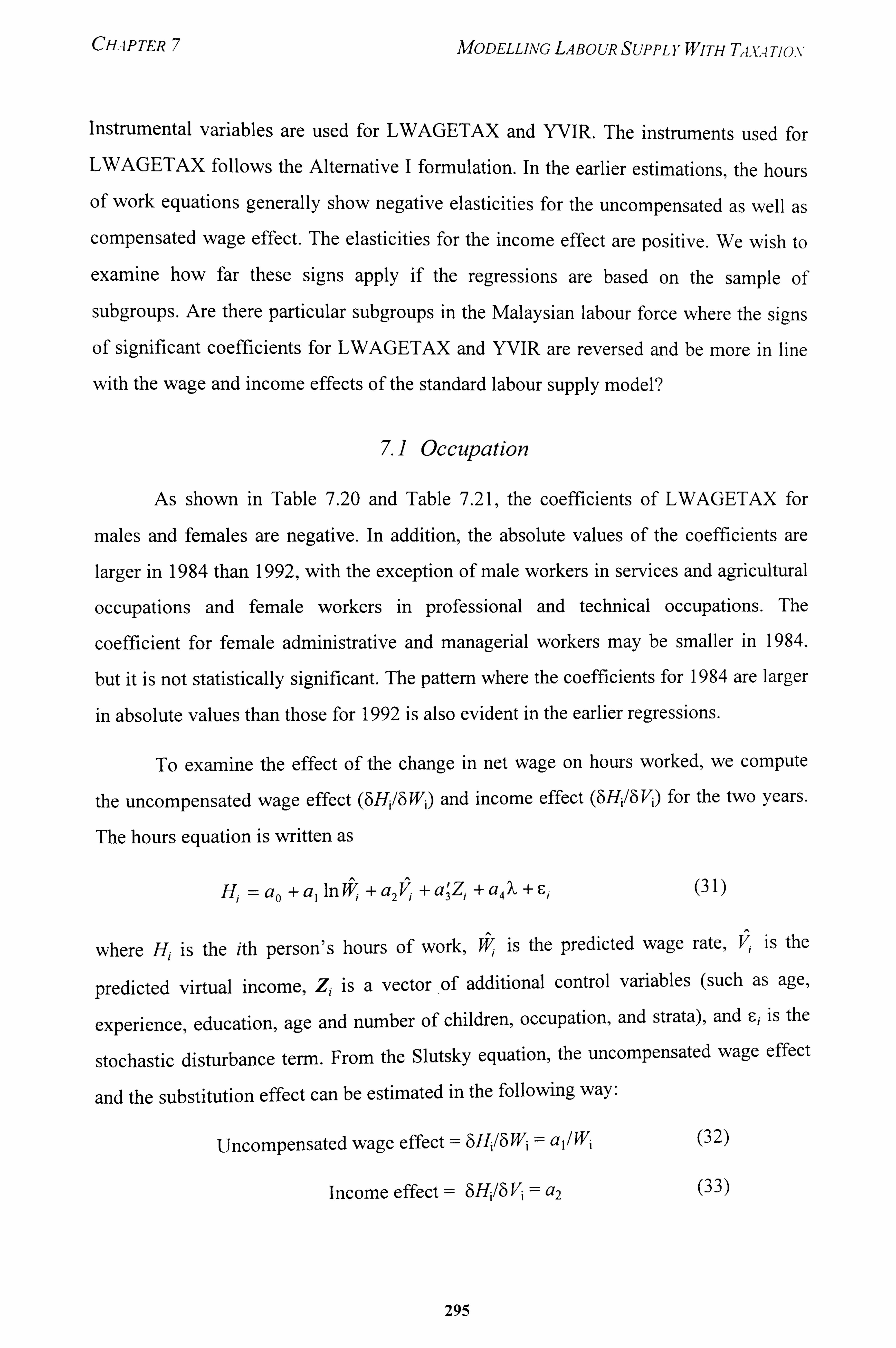
CHAPTER 7 MODELLiNG LABOUR SUPPL YWiTH T, 4-V. 4 TION

Instrumental variables are used for LWAGETAX and YVIR. The instruments used for LWAGETAX follows the Alternative I formulation. In the earlier estimations., the hours

of work equations generally show negative elasticities for the uncompensated as well as compensated wage effect. The elasticities for the income effect are positive. We wish to

examine how far these signs apply if the regressions are based on the sample of

subgroups. Are there particular subgroups in the Malaysian labour force where the signs

of significant coefficients for LWAGETAX and YVIR are reversed and be more in line

with the wage and income effects of the standard labour supply model?

7.1 Occupation

As shown in Table 7.20 and Table 7.21 , the coefficients of LWAGETAX for

males and females are negative. In addition, the absolute values of the coefficients are

larger in 1984 than 1992, with the exception of male workers in services and agricultural

occupations and female workers in professional and technical occupations. The

coefficient for female administrative and managerial workers may be smaller in 1984,

but it is not statistically significant. The pattern where the coefficients for 1984 are larger

in absolute values than those for 1992 is also evident in the earlier regressions.

To examine the effect of the change in net wage on hours worked, we compute

the uncompensated wage effect (8Hj16Wj) and income effect (6Hj16Vj) for the two years.

The hours equation is written as

H, =ao+ a, InW, + a V, +aZ, + a k+F, (31) 234i

where Hi is the ith person's hours of work, W, is the predicted wage rate, Vi is the

predicted virtual income, Zi is a vector of additional control variables (such as age,

experience, education, age and number of children, occupation, and strata), and Ej is the

stochastic disturbance term. From the Slutsky equation, the uncompensated wage effect

and the substitution effect can be estimated in the following way:

Uncompensated wage effect = 6Hj16 Wi =aI/ Wi (32)

Income effect = 6Hj18 Vi = a2 (33)

295

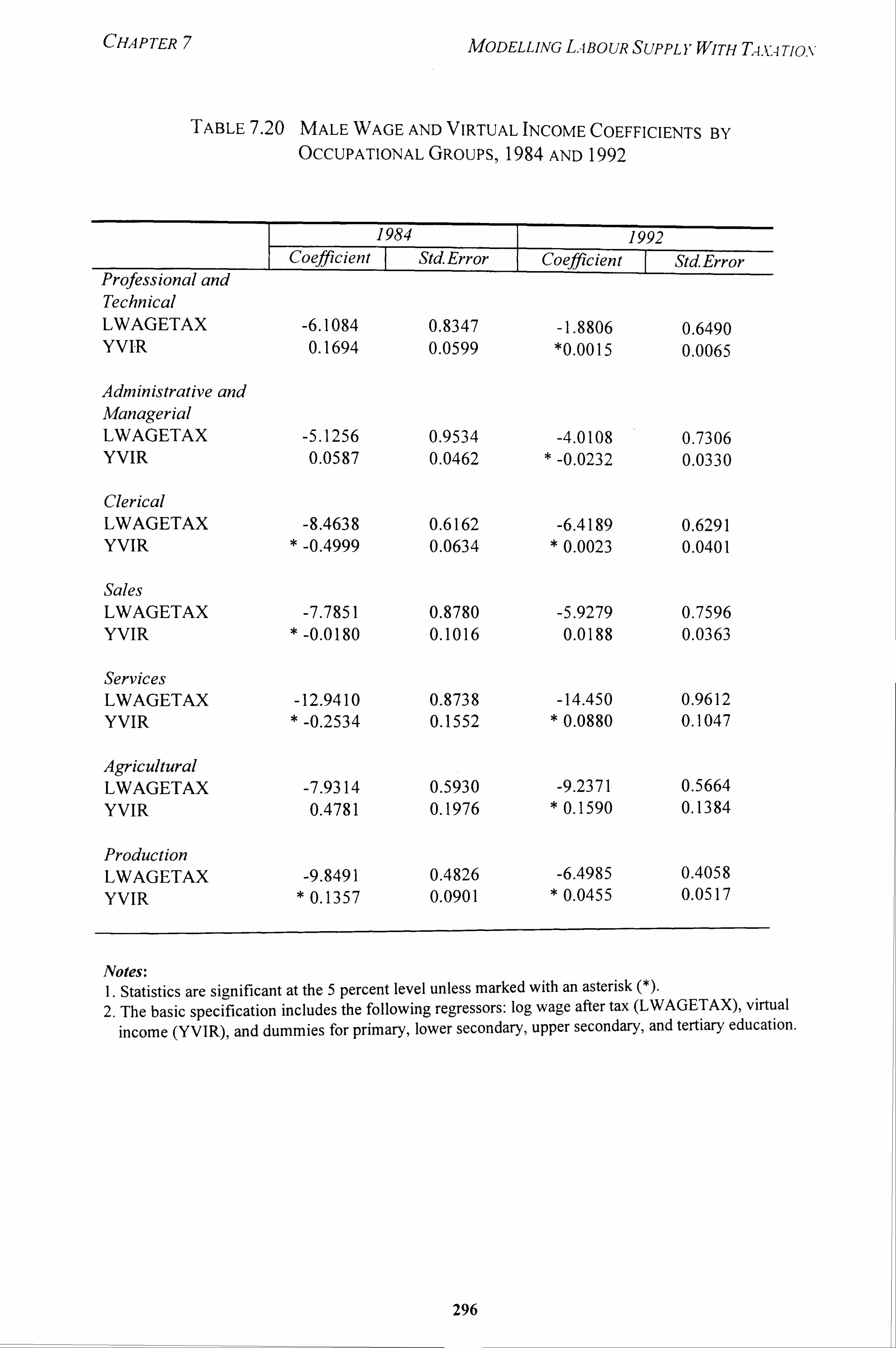
CHAPTER MODELUNG L. IBOUR SUPPL YWITH T4. v4 TION

TABLE 7.20 MALE WAGE AND VIRTUAL INCOME COEFFICIENTS BY OCCUPATIONAL GROUPS, 1984 AND 1992

1984 1992 Coefficient StdError Coefficie-nt--T- Std. Error

Professional and Technical LWAGETAX -6.1084 0.8347 -1.8806 0.6490 YVIR 0.1694 0.0599 *0-00 15 0.0065

Administrative and Managerial LWAGETAX -5.1256 0.9534 -4.0108 0.7306 YVIR 0.0587 0.0462 -0.0232 0.0330

Clerical LWAGETAX -8.4638 0.6162 -6.4189 0.6291 YVIR -0.4999 0.0634 0.0023 0.0401

Sales LWAGETAX -7.7851 0.8780 -5.9279 0.7596 YVIR -0.0 180 0.1016 0.0188 0.0363

Services LWAGETAX -12.9410 0.8738 -14.450 0.9612 YVIR * -0.2534 0.1552 0.0880 0.1047

Agricultural LWAGETAX -7.9314 0.5930 -9.2371 0.5664 YVIR 0.4781 0.1976 * 0.1590 0.1384

Production LWAGETAX -9.8491 0.4826 -6.4985 0.4058 YVIR * 0.1357 0.0901 * 0.0455 0.0517

Notes: 1. Statistics are significant at the 5 percent level unless marked with an asterisk 2. The basic specification includes the following regressors: log wage after tax (LWAGETAX), virtual

income (YVIR), and dummies for primary, lower secondary, upper secondary, and tertiary education.

296

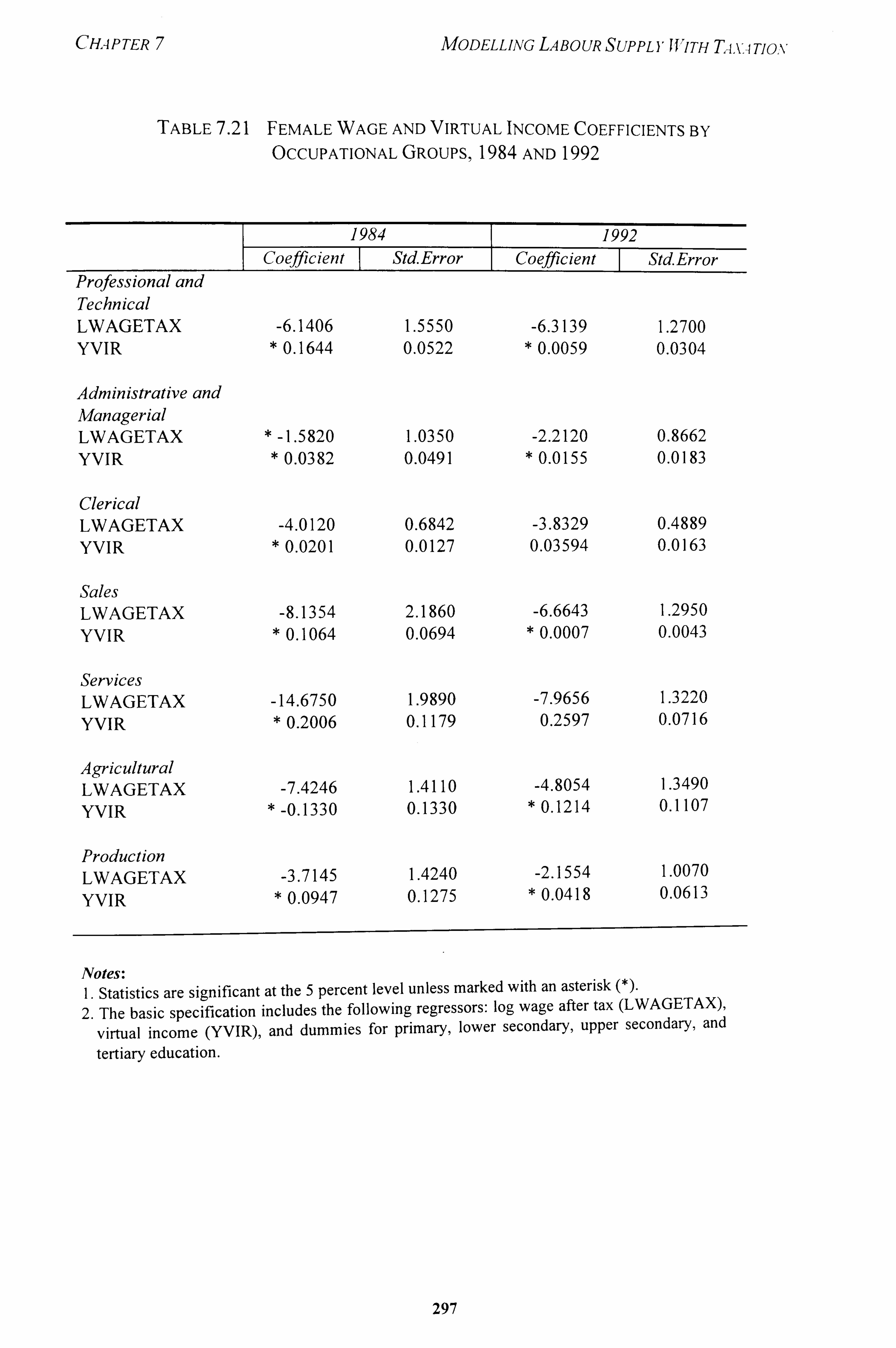
CHAPTER MODELLING LABOUR SUPPLYJVITH TA, u Tjo. v

TABLE 7.21 FEMALE WAGE AND VIRTUAL INCOME COEFFICIENTS BY OCCUPATIONAL GROUPS, 1984 AND 1992

Technical

Std. Error

LWAGETAX -6.1406 1.5550 -6.3139 1.2700 YVIR * 0.1644 0.0522 * 0.0059 0.0304

Administrative and Managerial LWAGETAX -1.5820 1.0350 -2.2120 0.8662 YVIR 0.0382 0.0491 0.0155 0.0183

Clerical LWAGETAX -4.0120 0.6842 -3.8329 0.4889 YVIR 0.0201 0.0127 0.03594 0.0163

Sales LWAGETAX -8.1354 2.1860 -6.6643 1.2950 YVIR * 0.1064 0.0694 * 0.0007 0.0043

Services LWAGETAX -14.6750 1.9890 -7.9656 1.3220 YVIR 0.2006 0.1179 0.2597 0.0716

Agricultural LWAGETAX -7.4246 1.4110 -4.8054 1.3490 YVIR * -0.1330 0.1330 * 0.1214 0.1107

Production LWAGETAX -3.7145 1.4240 -2.1554 1.0070

YVIR 0.0947 0.1275 0.0418 0.0613

Notes: 1. Statistics are significant at the 5 percent level unless marked with an asterisk

2. The basic specification includes the following regressors: log wage after tax (LWAGETAX),

virtual income (YVIR), and dummies for primary, lower secondary, upper secondary, and

tertiary education.

297

CHAPTER MODELLING LABOUR SUPPLYWITH T4, VA TIOY

In the discussion that follows, we will merely be examining the uncompensated

wage effect by occupation and education which area shown in Table 7.22 and Table 7.25 because the income effect is less interesting because they are generally insignificant. In 1984, the uncompensated wage effects are strongest for males who are engaged in

agriculture (-2.7), production (-2.8) and services (-3.3), while they are weakest for males

who were administrative and managerial workers (-0.3) and professional and technical

workers (-0.5). The calculated mean net wage rates for males are lowest for service

workers (RM3.80), agricultural workers (RM2.90) and production workers (RM3.40)

. and highest for managerial and administrative workers (RM 15.70) as well as professional

and technical workers (RM1 1.80). This implies that workers in agriculture, production,

and services occupations, which have much lower mean wage, increase their hours of

work much more in response to a reduction in wage compared with males in the

administrative, managerial, professional and technical occupations, who enjoy higher

wage rates.

Among the females, the negative uncompensated wage effects are strongest

among occupations with the lowest paying jobs as well. In 1984, the uncompensated

wage effects are strongest for female workers in sales (-7.0), services (-10.6) and

agriculture (-12.3) and weakest for females in administrative and managerial occupations

(417). The calculated mean net wage was RM9.20 per hour for female administrative

and managerial workers in 1984 compared with less than RM1.30 per hour in sales,

services and agricultural occupations.

The uncompensated wage effects for 1992 for both sexes are below the 1984

position, implying that changes in net wage in 1992 have a smaller effect on hours

supplied compared with 1984. The only exception to the decline is males in agriculture

which saw a slight increase in the uncompensated wage effect. The most dramatic

decline are recorded by females in sales, services and agricultural occupations where the

uncompensated wage effect in 1992 are less than half their values in 1984.

298

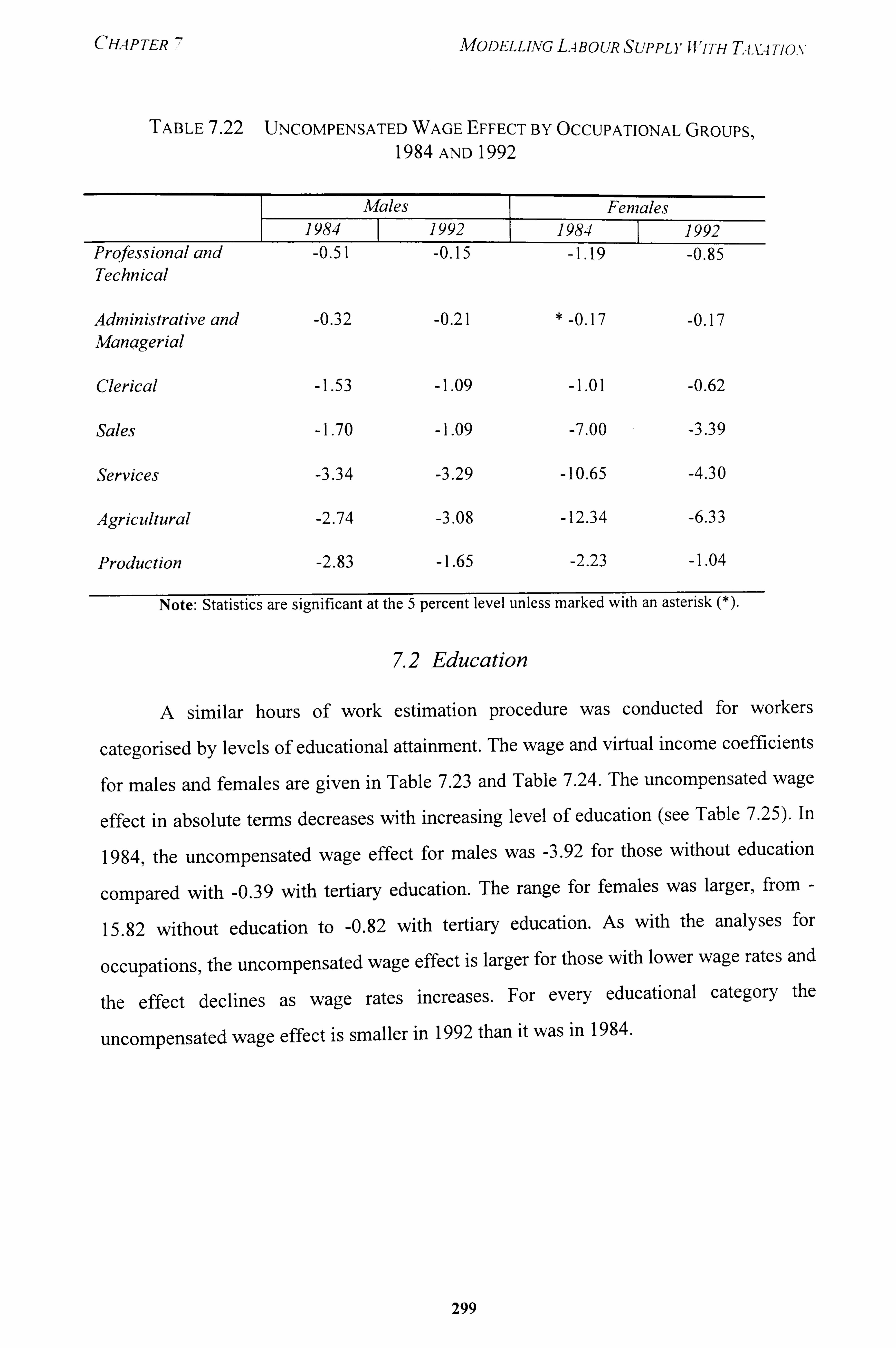
CHA P TER ', 1 MODELLiNG L. 4BOUR SUPPLY[f 7"iTH T-i. V-1 TION

TABLE 7.22 UNCOMPENSATED WAGE EFFECT BY OCCUPATIONAL GROUPS, 1984 AND 1992

Males Females 1984 1992 1984 1992

Professional and -0.51 -0.15 -1.19 -0.85 Technical

Administrative and -0.32 -0.21 -0.17 -0.17 Managerial

Clerical -1.53 -1.09 -1.01 -0.62

Sales -1.70 -1.09 -7.00 -3.39

Services -3.34 -3.29 -10.65 -4.30

Agricultural -2.74 -3.08 -12.34 -6.33

Production -2.83 -1.65 -2.23 -1.04


7.2 Education

A similar hours of work estimation procedure was conducted for workers

categorised by levels of educational attainment. The wage and virtual income coefficients

for males and females are given in Table 7.23 and Table 7.24. The uncompensated wage

effect in absolute terms decreases with increasing level of education (see Table 7.25). In

1984, the uncompensated wage effect for males was -3.92 for those without education

compared with -0.39 with tertiary education. The range for females was larger, from -

15.82 without education to -0.82 with tertiary education. As with the analyses for

occupations, the uncompensated wage effect is larger for those with lower wage rates and

the effect declines as wage rates increases. For every educational category the

uncompensated wage effect is smaller in 1992 than it was in 1984.

299

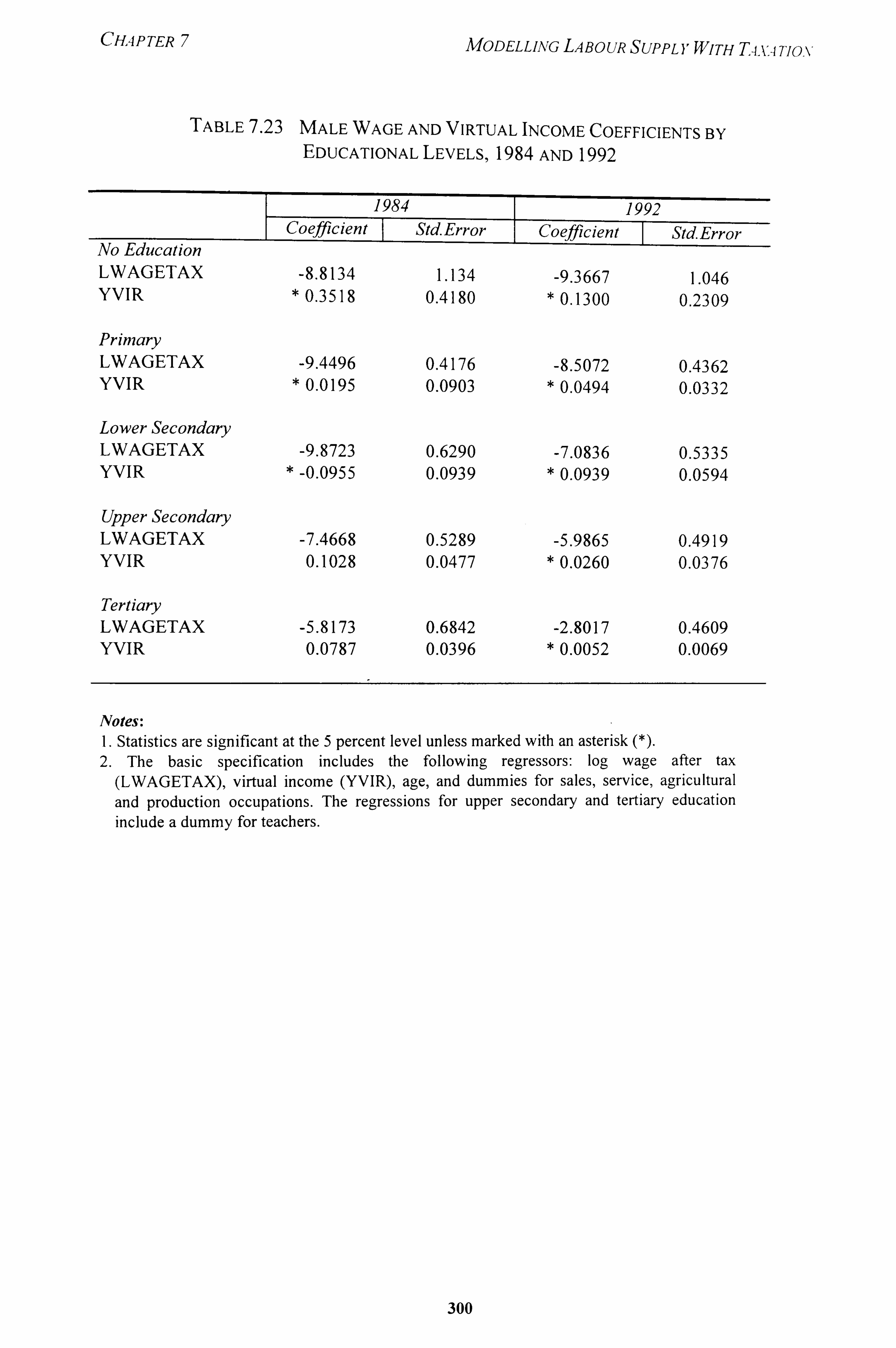
CHAPTER 7 MODELLiAG LABOUR SUPPLYWITH T4x. 4 Tiox

TABLE 7.23 MALE WAGE AND VIRTUAL INCOME COEFFICIENTS BY EDUCATIONAL LEVELS, 1984 AND 1992

1992 Std. Error

LWAGETAX -8.8134 1.134 -9.3667 1.046 YVIR * 0.3518 0.4180 * 0.1300 0.2309

Primary LWAGETAX -9.4496 0.4176 -8.5072 0.4362 YVIR 0.0195 0.0903 * 0.0494 0.0332

Lower Secondary LWAGETAX -9.8723 0.6290 -7.0836 0.5335 YVIR -0.0955 0.0939 * 0.0939 0.0594

Upper Secondary LWAGETAX -7.4668 0.5289 -5.9865 0.4919 YVIR 0.1028 0.0477 * 0.0260 0.0376

Tertiary LWAGETAX -5.8173 0.6842 -2.8017 0.4609 YVIR 0.0787 0.0396 * 0.0052 0.0069

Notes: 1. Statistics are significant at the 5 percent level unless marked with an asterisk 2. The basic specification includes the following regressors: log wage after tax

(LWAGETAX), virtual income (YVIR), age, and dummies for sales, service, agricultural and production occupations. The regressions for upper secondary and tertiary education include a dummy for teachers.

300

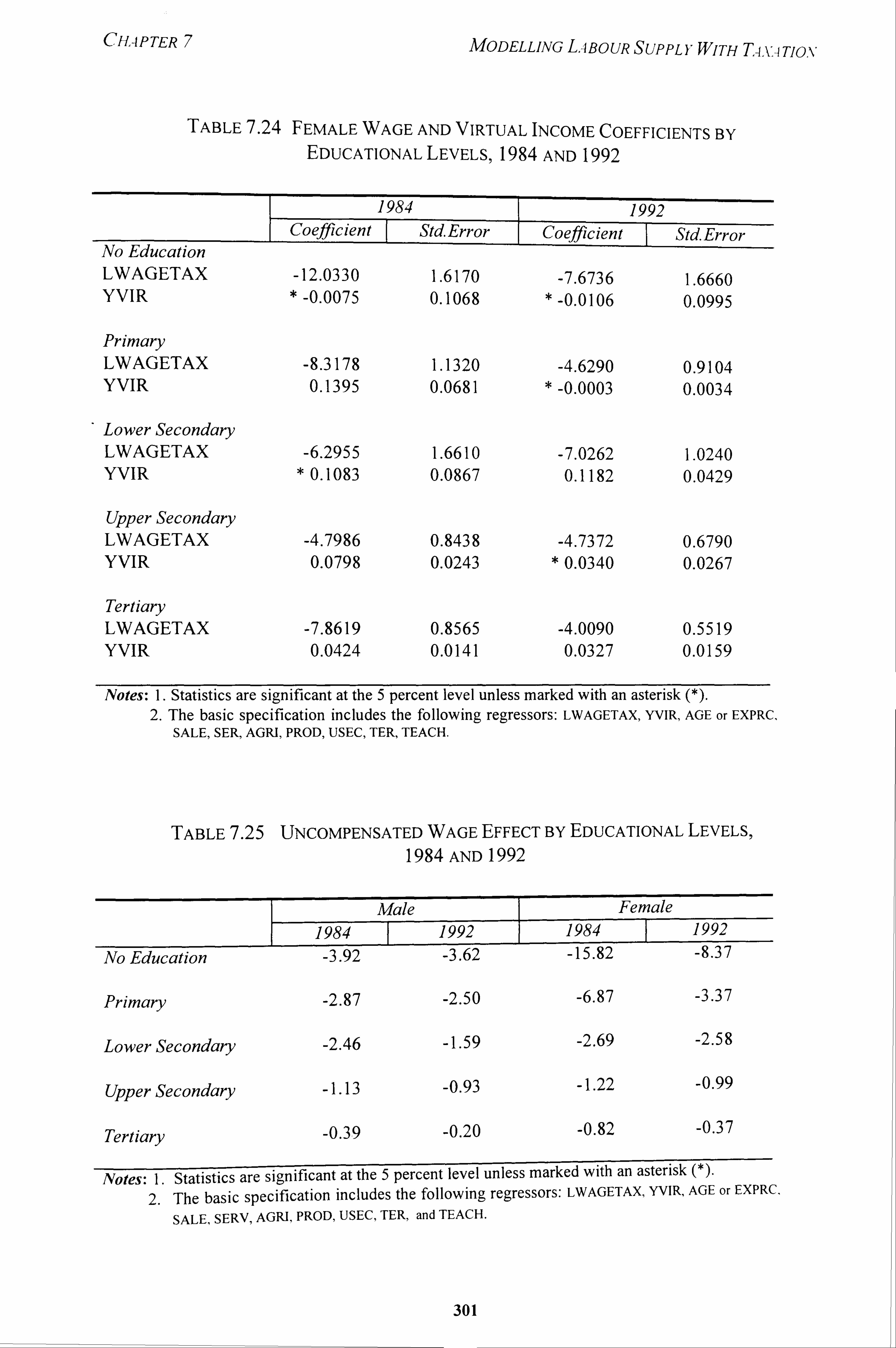
CHAPTER MODELLiNG LABOUR SUPPL YWiTH T-i, u Tjo. v

TABLE 7.24 FEMALE WAGE AND VIRTUAL INCOME COEFFICIENTS BY EDUCATIONAL LEVELS, 1984 AND 1992

No Education LWAGETAX YVIR

Primary LWAGETAX YVIR

Lower Secondary LWAGETAX YVIR

Upper Secondary LWAGETAX YVIR

1984 Coefficient Std. Error

-12.0330 1.6170 * -0.0075 0.1068

1992 Coefficient -StdError

-7.6736 1.6660 -0.0106 0.0995

-8.3178 1.1320 -4.6290 0.9104 0.1395 0.0681 -0-0003 0.0034

-6.2955 1.6610 -7.0262 1.0240 * 0.1083 0.0867 0.1182 0.0429

-4.7986 0.8438 -4.7372 0.6790 0.0798 0.0243 0.0340 0.0267

Tertiary LWAGETAX -7.8619 0.8565 -4.0090 0.5519 YVIR 0.0424 0.0141 0.0327 0.0159

Notes: 1. Statistics are significant at the 5 percent level unless marked with an asterisk (*). 2. The basic specification includes the following regressors: LWAGETAX, YVIR, AGE or EXPRC,

SALE, SER, AGRI, PROD, USEC, TER, TEACH.

TABLE 7.25 UNCOMPENSATED WAGE EFFECT By EDUCATIONAL LEVELS, 1984 AND 1992

Male Female 1984 1.992 1984 1992

No Education -3.92 -3.62 -15.82 -8.37

Primary -2.87 -2.50 -6.87 -3.37

Lower Secondary -2.46 -1.59 -2.69 -2.58

Upper Secondary -1.13 -0.93 -1.22 -0.99

Tertiary -0.39 -0.20 -0.82 -0.37

Notes: 1. Statistics are significant at the 5 percent level unless marked with an asterisk (*).

2. The basic specification includes the following regressors: LWAGETAX, YVIR, AGE or EXPRC,

SALE, SERV, AGRI, PROD, USEC, TER, and TEACH.

301

CHAPTER 7 MODELLjNG LA BO UR SUPPL Y WITH T4. V. 4 TION

7.3 Employee and Seýf-Emplqyed

The final set of hours of work equations were estimated for employee as well as for the self-employed and unpaid family workers using the three stage estimation procedure. The purpose of the exercise was to ascertain if this subgrouping of workers

would make a difference to the signs in the coefficients. Although the magnitude of

coefficients are generally greater for the self-employed and unpaid family workers than for employees, as Table 7.26 indicates the signs for LWAGETAX and YVIR remain

similar to the results obtained from earlier estimations, and the uncompensated as well as the compensated wage elasticities are negative.

8. DiscussioN

In the preceding sections, we performed some baseline estimations using the second

generation Procedure VIII three stage approach for married male and female heads of

households within the 20-54 years age group. In addition, we carried out four categories

of alternative estimations, namely, (a) hours of work without instrumental variables, (b)

three stage estimation for those working between 25-60 hours a week, (c) pre-tax hours

of work, and (d) regressions by occupation, education and employment categories. In

these estimations,, two major features emerge. First, taxes are found to have very weak

effects for the hours of work equation. This finding corresponds with other studies such

as Koster (1967), MaCurdy, Green and Paarsch (1990), and Mroz (1987). Therefore, the

decision to treat labour supply as exogenous in Chapter 5 for the tax reform simulations

can be supported by the findings in this chapter.

Second, the uncompensated and the compensated wage effect estimates are found

to be negative while the income effect estimates are positive for all estimates where the

coefficients obtained are significant. These signs seem to be contrary to what is normally

expected in the formal labour supply theory which states that the income effect is

negative and the wage effect is positive. This need not necessarily be the case in

empirical work though.

302

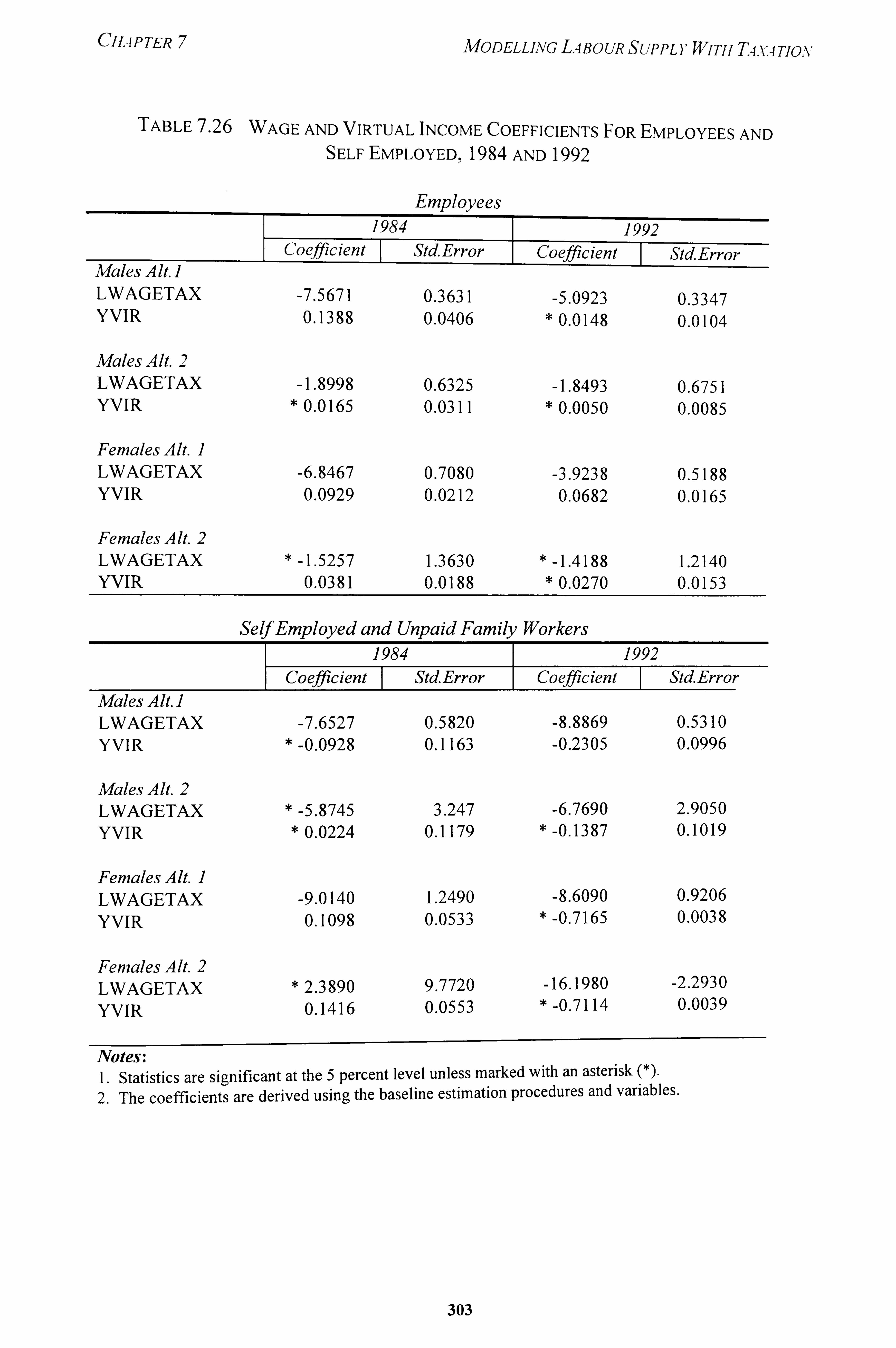
CHAPTER MODELLING LA BOUR SUPPL)'WiTH T4. v. 4 Tjav

TABLE 7.26 WAGE AND VIRTUAL INCOME COEFFICIENTS FOR EMPLOYEES AND SELF EMPLOYED, 1984 AND 1992

Employees 1992

StdError

LWAGETAX -7.5671 0.3631 -5.0923 0.3347 YVIR 0.1388 0.0406 * 0.0148 0.0104

Males Alt. 2 LWAGETAX -1.8998 0.6325 -1.8493 0.6751 YVIR 0.0165 0.0311 * 0.0050 0.0085

Females Alt. I LWAGETAX -6.8467 0.7080 -3.9238 0.5188 YVIR 0.0929 0.0212 0.0682 0.0165

Females Alt. 2 LWAGETAX -1.5257 1.3630 -1.4188 1.2140 YVIR 0.0381 0.0188 0.0270 0.0153

Self Employed and Unpaid Family Workers

Std. Error

LWAGETAX -7.6527 0.5820 -8.8869 0.5310 YVIR * -0.0928 0.1163 -0.2305 0.0996

Males Alt. 2 LWAGETAX * -5.8745 3.247 -6.7690 2.9050 YVIR * 0.0224 0.1179 * -0.1387 0.1019

Females Alt. I LWAGETAX -9.0140 1.2490 -8.6090 0.9206 YVIR 0.1098 0.0533 -0.7165 0.0038

Females Alt. 2 LWAGETAX 2.3890 9.7720 -16.1980 -2.2930 YVIR 0.1416 0.0553 * -0.7114 0.0039

Notes: 1. Statistics are significant at the 5 percent level unless marked with an asterisk 2. The coefficients are derived using the baseline estimation procedures and variables.

303

CHAPTER MODELLING LABOUR SUPPLYWITH Ti. u Tio. v

There are three aspects to our discussion. First, we cite other studies with similar results. Second, we explore some reasons why the results seem reasonable in the Malaysian context, and finally, we discuss the limitations. of data and model specification

that could affect the regression results.

1 Studies With Similar Results

In some of the earlier studies in the United States based on data from the 1960

Census of Population and the 1967 Survey of Economic -Opportunity, there are some

evidence on the negatively- sloped labour supply curve. The slope of the male hours of

work function was found to be more negative when the calculated wage rate was used

than when an alternative wage rate variable, such as an instrumented wage rate was

constructed (Bloch, 1973; DaVanzo, DeTray and Greenberg, 1973; Masters and

Garfinkel, 1977; Borjas, 1980). Even after efforts were made to remove spurious

correlation from the wage variable, most studies found a negative uncompensated own-

wage elasticity of hours of work at sample means. Pencavel (1986) points out that the

uncompensated wage elasticities for males can range between -0.15 and -0.09 for

DaVanzo, DeTray and Greenberg (1973), -0.110 for Masters and Garfinkel (1977) and -

0.156 for Ashenfelter and Heckman (1973). However, because of the strong negative

income effect, in many cases the estimated compensated wage elasticities in these studies

are positive. Evidently, this is not the case for Malaysia because from our estimations,

the income effect is found to be either very low or insignificant.

As for non-wage income, it is generally recognised that this variable is difficult to

measure accurately. The different procedures used generate distinctly different estimates

of the effect of non-wage income on hours of work. Pencavel (1986: 63) argues that only

16 of the 57 different coefficients presented in DaVanzo, DeTray and Greenberg's study

are statistically significant, and of these 16 estimates, exactly one-half is positive and

one-half is negative. Since the estimates on non-wage incomes vary so much and the

uncompensated wage effect is typically estimated to be negative, it is not unusual for the

substitution effect to be negative.

304

CHAPTER MODELLING LABOUR SETPLYWITH T4. u Tio, %r

Among the more recent studies using the instrumental variables approach, Mroz (1987) initially obtained a negative uncompensated wage elasticity by using the OLS but

which turns positive after he introduced instrumental variables for logged wage. In his

estimate of taxes in the single worker model, the coefficients obtained for logged wage are negative for all the six specifications. As for non-wife income, the coefficients are

negative for four of the specifications and positive when the labour market experience of females are used as instruments. The changing of signs are attributed to the different

exogeneity assumptions used in the alternative specifications. In another study, Flood

and MaCurdy (1992) obtained negative wage effect and positive income effect in one of

their specifications but they attribute it to the endogeneity of the gross wage and income

variables (and these variables squared) which are used as instruments for net wage.

Blomquist (1996: 387) raised some doubts on this issue and argued that although it is

difficult to test whether the gross wage rate and nonlabour income are admissible

instruments, in his Monte Carlo simulations of hours of work for small samples, the

instrumental variables using background variables show serious bias, especially in small

samples, compared with those using gross wage rate and non-labour income.

In our study, we have tried to address some of the concerns about endogeneity of

net wage as well as measurement error of hours. While the absolute value of the

coefficients for logged wage vary with the alternative specifications, the negative signs

remain. Given the very small, and often insignificant, positive income effect, this implies

that the substitution or the compensated wage effect (which is calculated as a residual) is

negative.

8.2 Are the Results Supportable?

One can raise the question whether the signs obtained from the Malaysian data set

seem reasonable given the socio-economic and institutional setting of Malaysia. A

scatterplot analysis of hours of work by log net wage for males and females in 1984 is

shown in Figure 7.14 and Figure 7.15. The charts show that there is a much wider spread

of hours worked at lower wages than at higher wages. The line of best fit shows a

negative relationship in both the cases.

305

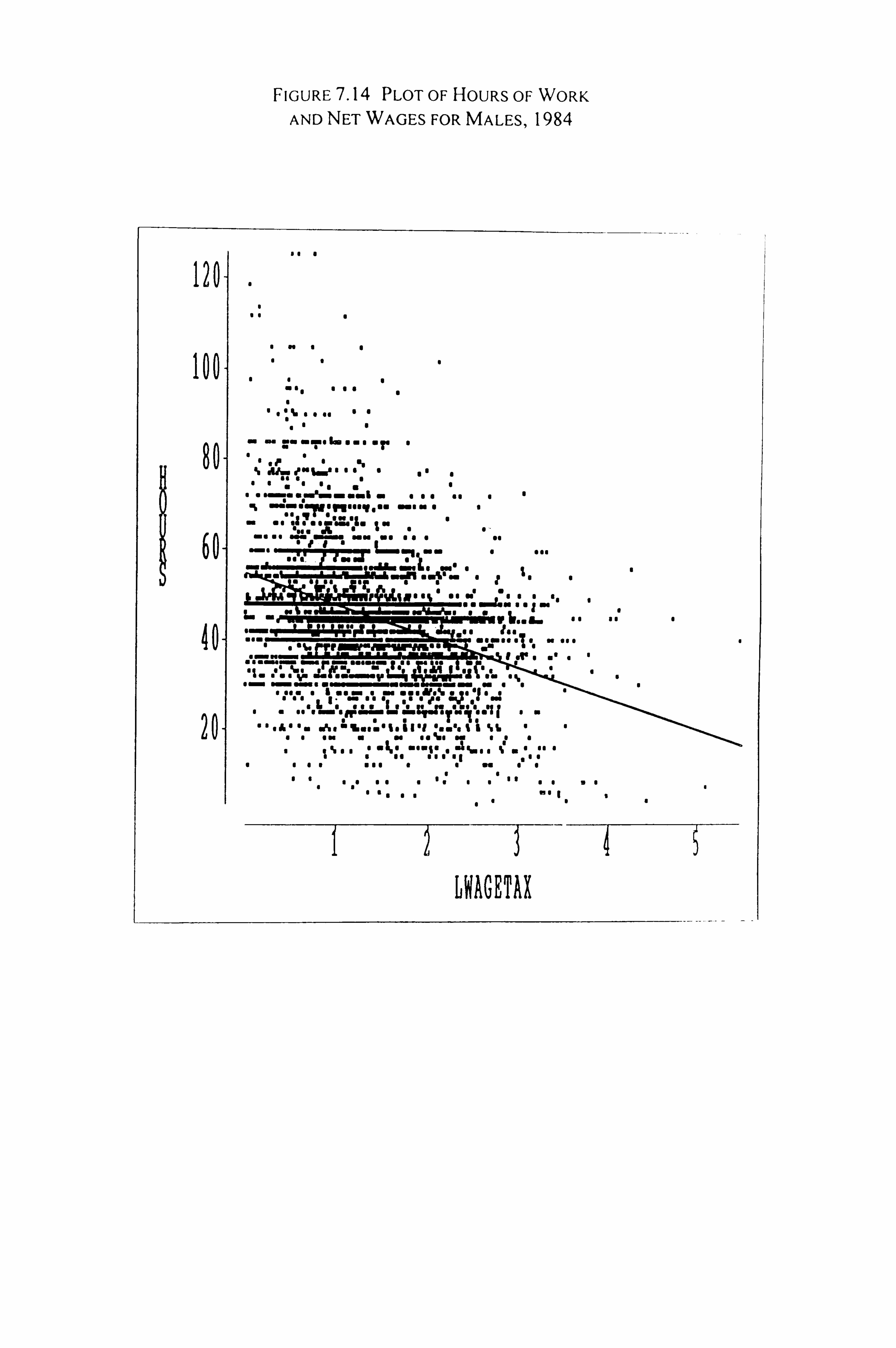
FIGURE 7.14 PLOT OF HOURS OF WORK

AND NET WAGES FOR MALES, 1984

ws =ev amme Imp aaa or 0

41 Also on %-ý aIa6 as 0a a8aIa

9 oýus...:: Mamg an aaaa10 10 ýme a resseffeen e

Pff: B1 al

.

.:. a ejiml) -%a0 -09 me of -- mn as aa0 41 1 L. sea Eýa GV fI we Sal a ane all vvw

ON L. me Loan@

a0

646_ was 1% Be a.. L

la! ., r. 9% aaaa kee U-4 IA

all 46 a sea a mom a ses ma@dV@% aL1; as as $I Bondi@ eye

... fre. es I., aleAs am Ae"llanemelellel 'sweet I %I,

W all 44%8 Mo IIa

a6 Mamie a l3avel I so a me 24a so

I

a

a

Iý-I

LWAGETH

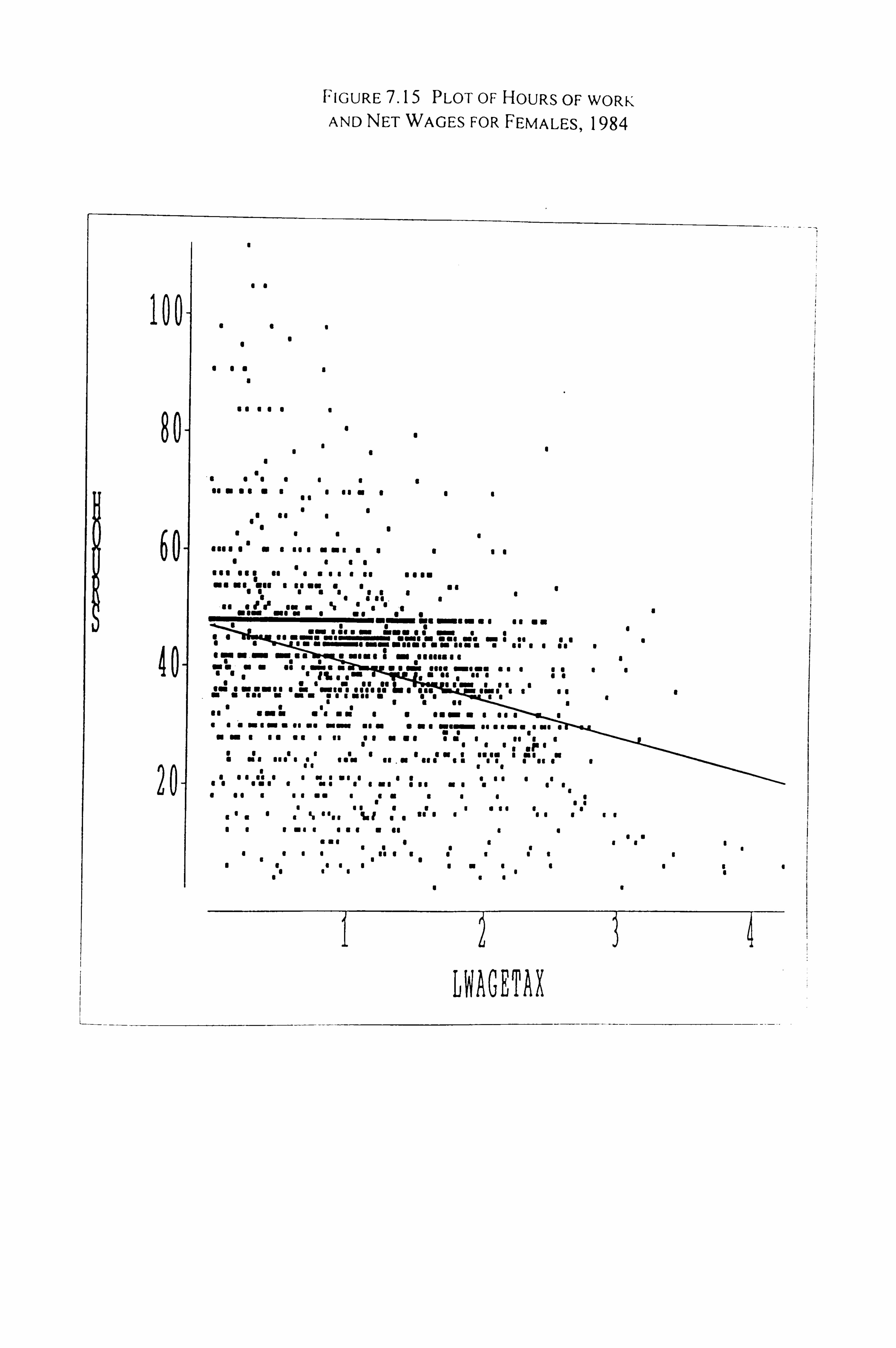
FIGURE 7.15 PLOT OF HOURS OF WORK AND NET WAGES FOR FEMALES, 1984

a

4a

I S I

I

U lu I I

sees Iaa as 10 no aaa

ago see as aa6aa Be seen a me as won a Be use aI as to a

as all? ow 0 go aaaa "am me aa we aa as an

am seený Mosilluse ý18 as SIMON waý am@ an use we me 9 of aI a sommýommuseng man seen a so aI of 9 M, ý as a 01110le

:m @@legal aa

WE a0 as a mine as as Mesa sees ýo Ma aIaaa94 a Me 4maa as 8 as aaI

aaJ of slim @Bonn I @I a am I an smog a an ýto I $@edge I @so IMMI@ II so an IS as$ a WINS as smog aaaII

IIIaIIa of a so Emu aa 11011 1a @am aI so aI 6aa wwouw= go an Mawn as as aaa maý as a am aa us 0

Me all I as an I Is IIa so is

me I of II a4a81

or, aIaIIII on I seem a me Me a us in@ aI too 21.01 as$ Is go a of aI

a of aI

a so as 91 as aaa4 as aI aa ago aaa No a so aaa to

6 of aaa an aaaaaIa aI

Is a916 of Ia

% in Iaa 'I IaI19 :II

we IIaIa so 44

one Iaa son

619a

I to Ia02

OR

4

a

I I

S

LWAGETAX

4

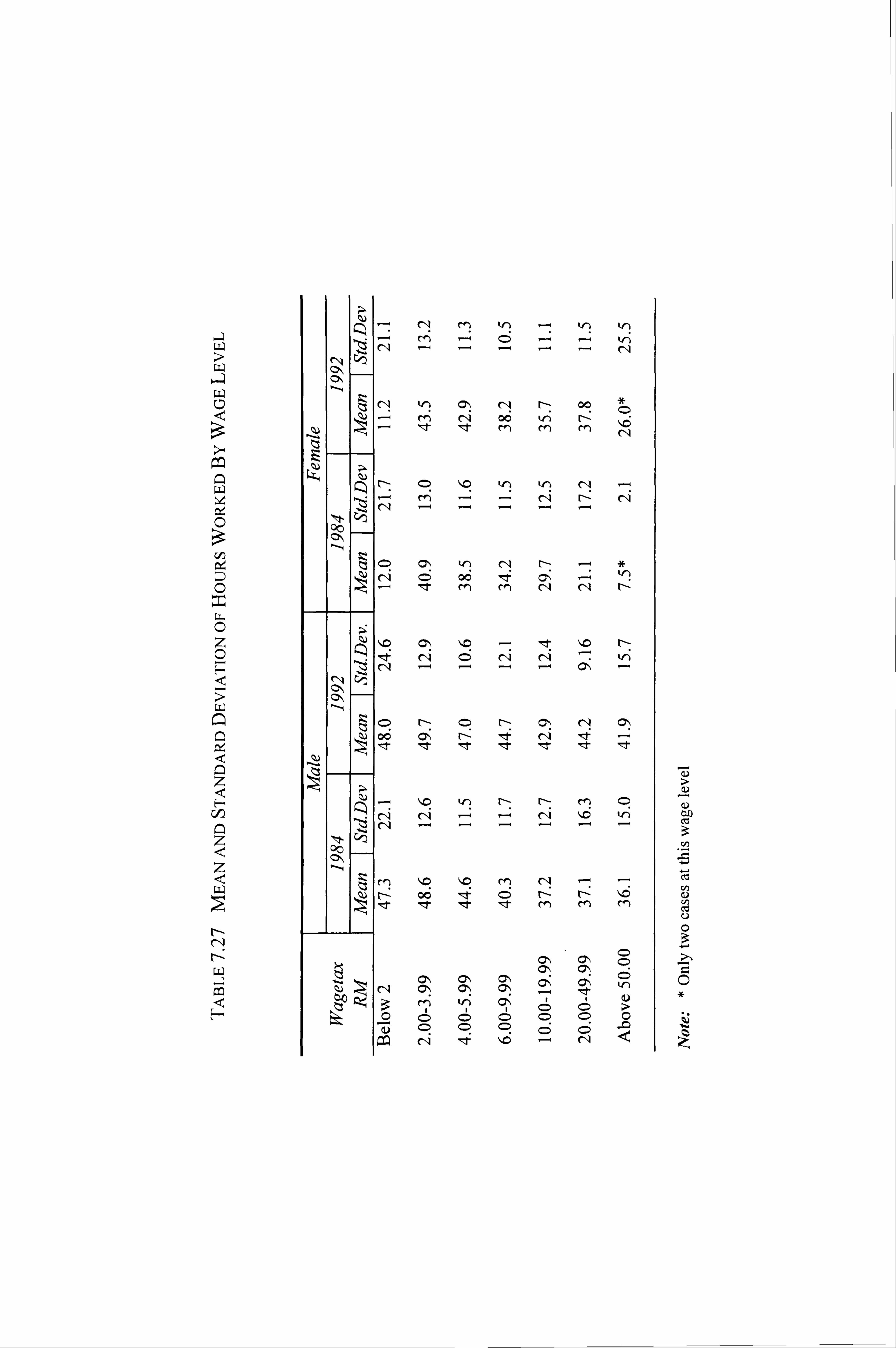
LL >

0

Cýl M kr) kr) kn

r-- 00

o6 Vý r-ý mm rf)

r- ---

-----

kn

INC)

C> C)

"0 V_ý r- r- rn CD

r1r) 110 110 M r1l --q 00

Itt Itl- I- I- mmm

rf) tr) C> <ý cý (Z

u Z

cý

rý

cý CD

-zý

cý CD

c;

25 (=;

-

CD cý

r-q

0

cz cz u 0

0

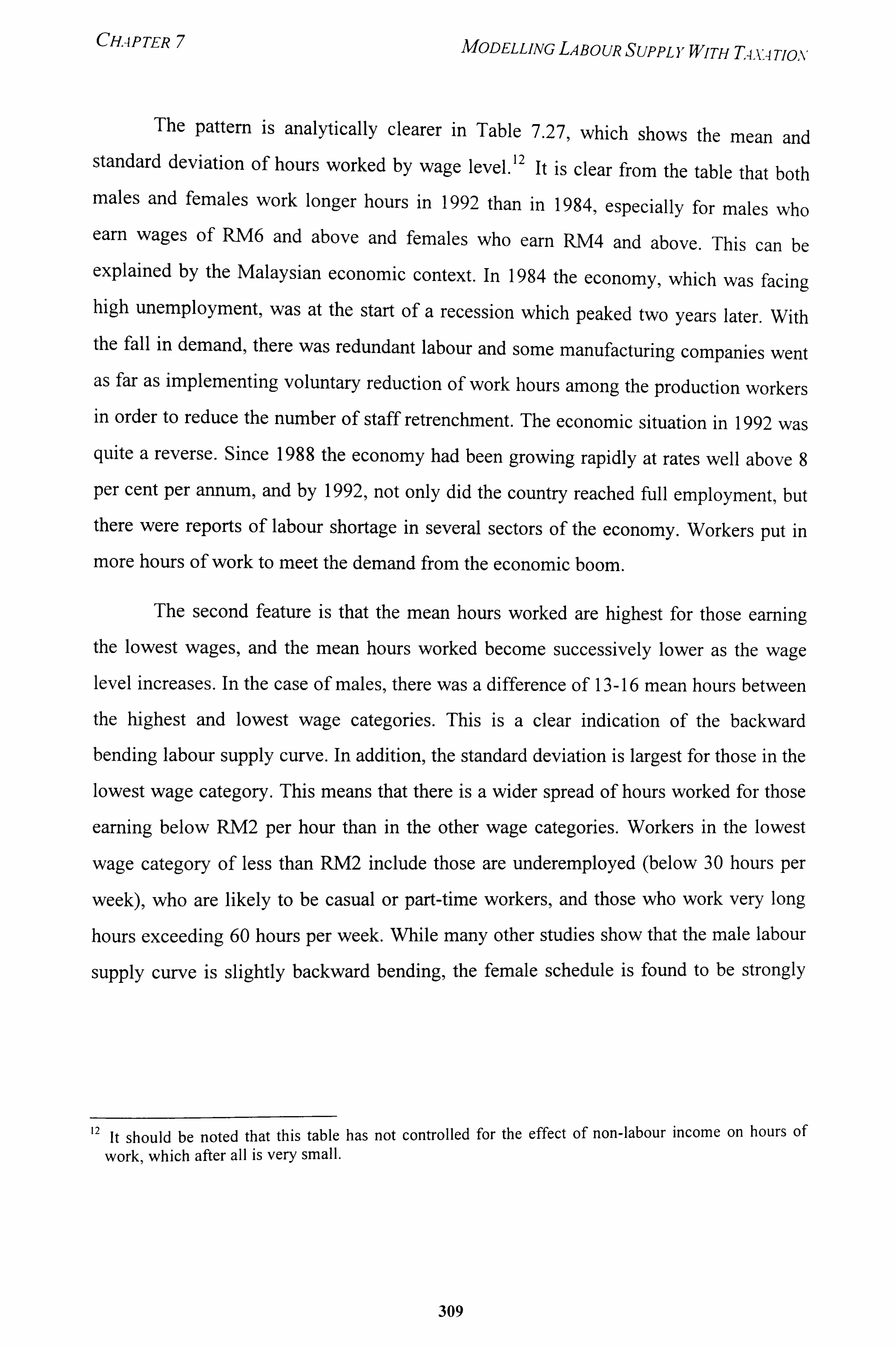
CHAPTER MODELLiNG LABOUR SUPPL YWITH T4-u Tiox

The pattern is analytically clearer in Table 7.27, which shows the mean and standard deviation of hours worked by wage level. 12 It is clear from the table that both males and females work longer hours in 1992 than in 1984, especially for males who earn wages of RM6 and above and females who earn RM4 and above. This can be explained by the Malaysian economic context. In 1984 the economy, which was facing high unemployment, was at the start of a recession which peaked two years later. With

the fall in demand, there was redundant labour and some manufacturing companies went as far as implementing voluntary reduction of work hours among the production workers in order to reduce the number of staff retrenchment. The economic situation in 1992 was quite a reverse. Since 1988 the economy had been growing rapidly at rates well above 8

per cent per annum, and by 1992, not only did the country reached full employment, but

there were reports of labour shortage in several sectors of the economy. Workers put in

more hours of work to meet the demand from the economic boom.

The second feature is that the mean hours worked are highest for those eaming

the lowest wages, and the mean hours worked become successively lower as the wage level increases. In the case of males, there was a difference of 13-16 mean hours between

the highest and lowest wage categories. This is a clear indication of the backward

bending labour supply curve. In addition, the standard deviation is largest for those in the

lowest wage category. This means that there is a wider spread of hours worked for those

earning below RM2 per hour than in the other wage categories. Workers in the lowest

wage category of less than RM2 include those are underemployed (below 30 hours per

week), who are likely to be casual or part-time workers, and those who work very long

hours exceeding 60 hours per week. While many other studies show that the male labour

supply curve is slightly backward bending, the female schedule is found to be strongly

12 It should be noted that this table has not controlled for the effect of non-labour income on hours of work, which after all is very small.

309

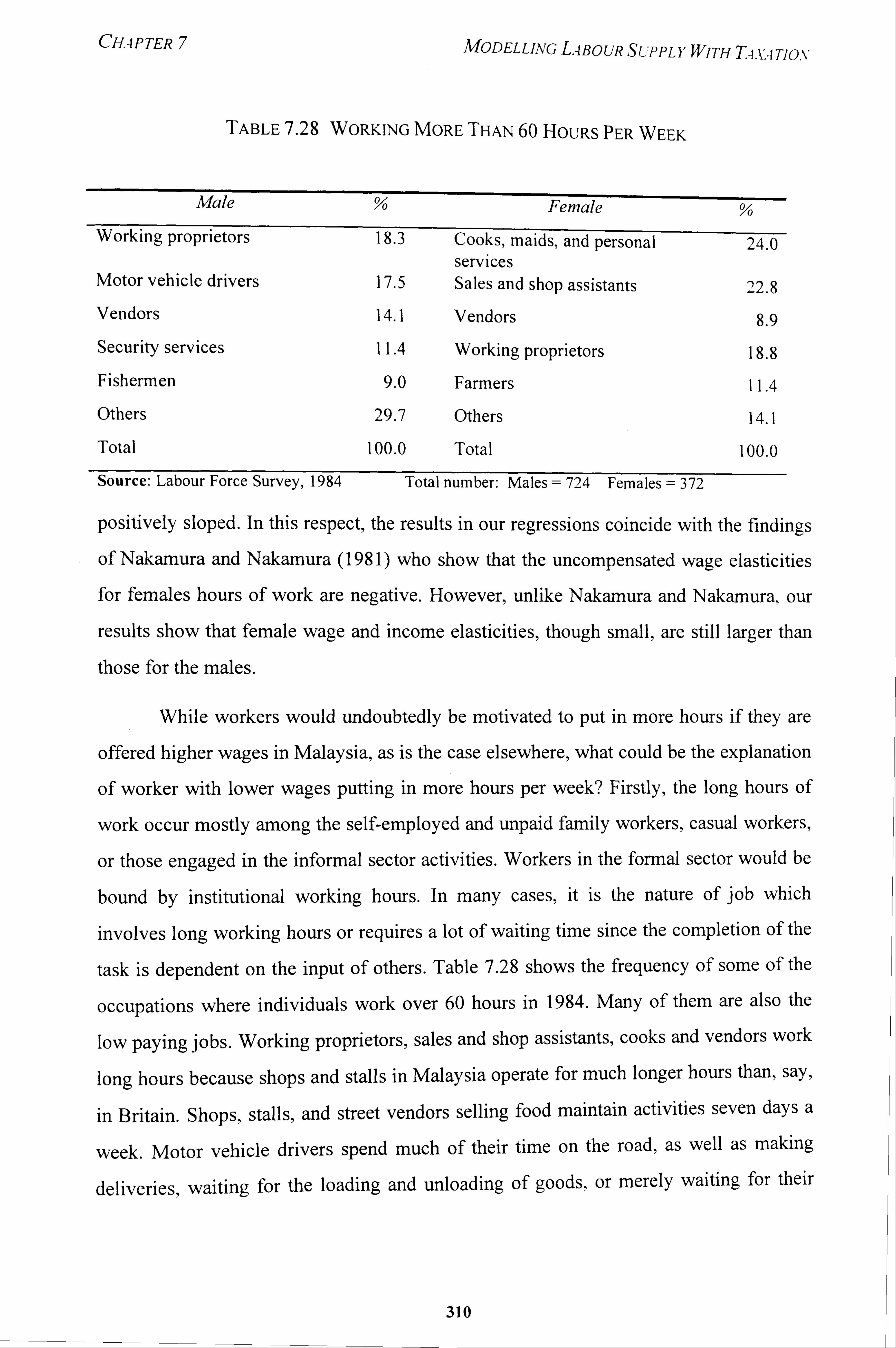
CHAPTER 7 MODELLiNG LABOUR SUPPLYWITH TA-v. 4 Tiav

TABLE 7.28 WORKING MORE THAN 60 HOURS PER WEEK

Male % Female % Working proprietors 18.3 Cooks, maids, and personal 24.0

services Motor vehicle drivers 17.5 Sales and shop assistants 212.8 Vendors 14.1 Vendors 8.9 Security services 11.4 Working proprietors 18.8 Fishermen 9.0 Farmers 11.4 Others 29.7 Others 14.1

Total 100.0 Total 100.0

Source: Labour Force Survey, 1984 Total number: Males = 724 Females 372

positively sloped. In this respect,, the results in our regressions coincide with the findings

of Nakamura and Nakamura (198 1) who show that the uncompensated wage elasticities

for females hours of work are negative. However, unlike Nakamura and Nakamura, our

results show that female wage and income elasticities, though small, are still larger than

those for the males.

While workers would undoubtedly be motivated to put in more hours if they are

offered higher wages in Malaysia, as is the case elsewhere, what could be the explanation

of worker with lower wages putting in more hours per week? Firstly, the long hours of

work occur mostly among the self-employed and unpaid family workers, casual workers,

or those engaged in the informal sector activities. Workers in the formal sector would be

bound by institutional working hours. In many cases, it is the nature of job which

involves long working hours or requires a lot of waiting time since the completion of the

task is dependent on the input of others. Table 7.28 shows the frequency of some of the

occupations where individuals work over 60 hours in 1984. Many of them are also the

low paying jobs. Working proprietors, sales and shop assistants, cooks and vendors work

long hours because shops and stalls in Malaysia operate for much longer hours than, say,

in Britain. Shops, stalls, and street vendors selling food maintain activities seven days a

week. Motor vehicle drivers spend much of their time on the road, as well as making

deliveries, waiting for the loading and unloading of goods, or merely waiting for their

310

CHAPTER 7 MODELLiNG LABOUR SUPPLY WITH Tq, ýýi Tjo. v

services to be demanded. Maids and servants often live with their employers where their services would be provided during throughout the day. Fishermen who are out to sea would include the hours spent away from shore as their working hours. These workers are not paid on the hourly basis but on a monthly salary and/or on the number of tasks

performed. In view of the long working hours and low earnings associated with these

occupations, the calculated earnings per hour of the individuals in these occupations

would be very low.

Secondly, those with low wages and non-labour income will have to increase

their hours of work in order to reach an income level that can meet their household

consumption. Participation is typically high in a society without an unemployment

benefit system since the option of either working for low wages or to remain unemployed

and receive some benefit, is not open to individuals. The social norm dictates that all

able-bodied adult males are expected to work and cannot depend on family ties for

financial support beyond a certain length of time, unless under exceptional

circumstances. Without a comprehensive income support programme which would raise

family income to a certain subsistence level , it appears that those in the lower wage

categories would maximise their hours of work, if there is a opportunity to do so, in order

to reach their 'target' household income to meet their family financial obligations.

Workers in these wage category tend to be those with little or no education and often

work in occupations with little job security. They are largely self employed or engaged in

'informal' sector activities. The added worker effect is also more evident among families

with low income. As discussed in Section 6.1.2, women with low family income have a

higher likelihood of participation. These women are engaged in part-time work, while

still performing their household duties, in order to supplement their husbands' income.

Those with higher wages tend to be better educated and have better job security.

In addition, their hours of work tend to be institutionally determined. Government

employees work between 8 a. m. to 4.15 p. m. on a five and the half working week, while

office workers in the private sector work between 9 a. m. to 5 p. m. on a five day week

with shorter lunch hours. Workers on the highest wage rates have greater flexibility in

their working time, which is reflected in the larger standard deviation in their hours of

311

CHAPTER 7 MODELLjNG L. 4BOUR SUPPLYWITH T4. k4 Tim'

work. This could also mean that there are some workers earning high wage rates who work shorter hours as well as long hours. In view of the hours of work pattern described, it is not surprising in the Malaysian labour market to encounter a backward bending curve which starts from the very lowest income levels, rather than the higher income levels as described in formal microeconomic theory.

The assumption that leisure is a normal good, that is, higher income is related with increased demand for leisure and negatively related with hours of work, does not appear to be supported by the regression results. In any case, after controlling for net wages, the effect of non-labour income on hours of work is either very small or statistically insignificant. In the baseline regressions, the income elasticities for the males are practically zero except for Alternative I in 1984. For the females, there is a small positive income elasticities for 1984 and zero for 1992. There is a positive relationship, albeit small, between non-labour income and hours of work. One reason for this could be

that individuals in the prime working groups are be keen to build up their wealth position for retirement.

In the developed countries where the unemployed workers are paid a lump-sum

unemployment benefit, one of the issues to be investigated is whether the size of the

benefit is large enough for individuals to choose non-participation in preference to

participation since they would reach a higher utility level from voluntary unemployment.

The choice of the two alternatives would depend on the individual's marginal rate of

substitution between income and leisure relative to the wage rate. Another line of enquiry

is the case of a negative income tax which has been criticised by economists for its

negative effect on work incentives. The effect of government transfer programmes

introduce non-convexities in the budget line which could give rise to multiple tangencies

and small changes in the wage or tax parameters can lead to large changes in desired

hours of work. In addition, where movements between marginal tax brackets have

significant tax implications, there is an issue of the clustering of individuals around the

kinks on the budget line as a result of controlling their hours of work. To address this

clustering, analysts introduce the optimisation error in their model specification on the

argument that individuals cannot fine-tune their hours of work precisely.

312

CHAPTER MODELLiNG LABOUR SUPPL YWITH Ti. u TIO. %,

These issues, though interesting and relevant in the developed countries context, are unimportant for countries, such as Malaysia. The first two issues are irrelevant

because of the absence of unemployment benefit or negative income tax programmes. Regarding the third issue, there is little reason to believe that the number of individuals

who try to locate at the kinks are significant enough to warrant attention. The proportion

of taxpayers among those who work are small. Those who pay income taxes are in

relatively low tax brackets, where the median tax bracket in 1992 was 12 per cent for

both sexes. For the average taxpayer, it might not appear to be worth the trouble to limit

the hours of work. The primary concern is really to raise their total income rather than to

remain in a lower tax category by limiting hours of work. Furthermore, there is little

scope for them to vary the hours of work in order to locate at the kink because the bulk of

the income taxpayers are employees in the formal sector where the hours of work are

institutionally determined. Among those who are engaged in business or are self

employed, there must be other effective avenues of tax planning permitted under the

Income Tax Act rather than limiting their hours of work. For the reasons above, we do

not introduce the optimisation error in our model.

8.3 Model Specification and Data Limitations

In this chapter, we use the standard utility function to develop the models for

participation, wages, and hours of work for heads of households. The regression analyses

yield elasticity estimates for Malaysia, which could be compared to results of studies

conducted elsewhere. One issue that could be raised is whether the standard utility

function used for the model is flexible enough to accommodate the concept of

households requiring at least a minimum income level to meet their consumption needs,

which may be regarded as the fixed cost. For societies that do not have income support

programmes, household members would have to work long hours or take up part-time

work to supplement their household income in order to reach at least a 'target income'

level to cover the fixed cost. This may require a reformulation of the utility function to

capture the backward sloping supply curve of labour for households with low marginal

wage rates.

313

CHAPTER MODELLING LABOUR SUPPLYWITH T4x. A TIO. V

One alternative formulation that could accommodate the backward bending

labour supply curve is given in Blundell (1980), which we surnmarise below. The utility function of each household h is given by a strictly convex utility function,

(4XIhIMIhý X2WM2hý -.., XrhIMrhl (34)

where Xih is the quantity of good i consumed, and each deflator Mih measures the

corresponding specific effect on utility of household composition. Let pi denote the price

of good i and yh the income of household h, the cost function is given by

Ch(Pq Uh) Ch(PlMlhý P2M2hý ... 5 PrMrh5 Uh) (35)

where ah(p) and b(p) are concave, linear homogeneous functions in p. In the model, the

fixed cost ah(p) depend on household composition and a Cobb-Douglas is chosen for b(P)

in order to lead to the linear expenditure system. If there is a single male worker in each

family facing a marginal wage rate w and a linear budget constraint

p'x + wl = wT+y y (36)

where 1 is leisure time, T is the maximum time available, y is full income and y' is non-

labour income. Labour supply is given by T-I=h. As suggested by Muellbauer (1980),

the cost function in the form of equation (35) is as follows

1-0 0 Ch (Whý A Uh) = ah(P) + WAD) + b(p) Wh Uh (37)

where 0<0 <1 and d(p) is homogenous of degree zero in prices. To simplify, Blundell

specifies that

d(p) =y, fl pi", i'Di = 0, Yl>O ii

Pi

Taking derivatives ofChwith respect to price, the expenditure equations for all i are as

follows:

PiXih: ":: Pi7iMih + Yl8iWh + (I-O)Pi(Y'h + (T-d(P))Wh-ah(P)) (38)

314

CHAPTER MODELLiNG LABOUR SUPPLYWITH T4, v. -i Tio, v

The labour supply equation corresponding to equation (38) is given by

h=0 (a(p) - y') + (I - 0)(T - d(p)) (39) w

which has the property of being backward sloping for y' < a(p). In other words, the labour supply curve is backward sloping when the non-labour income is less than the fixed cost. In the sample of households in his study, Blundell found that this condition is

typically satisfied.

The second issue is that the static labour supply model does not take into account life cycle considerations. ' 3 In a life cycle model, an individual can decide on the number

of hours to supply to the market and the intensity of market participation can vary with

age. Given his long-run values of wealth and his wage, he must decide on the optimal

timing of hours and consumption, which vary over the life cycle. Therefore, there is a

difficulty with regard to the standard practice in empirical labour supply studies of using

an aggregate of all current period non-eamings income to estimate pure income effects.

However, the available data do not permit any attempt to separate out these life-cycle

considers to obtain wealth elasticities.

The data source is also not rich enough to capture the ideal theoretical concepts

that could be used to measure pure income effects. The problem of estimating the income

slopes in empirical work is evident in other studies in the developed countries as well. As

noted by Smith (1980: 166), 'The estimated income slopes were disappointing because

the income variable either had the wrong sign (positive), implying that leisure was an

inferior good, or it was sufficiently small so that compensated own-wage slopes in the

labor supply equation remained negative. ' Among the reasons to explain these failures

are the severe under-reporting of the income variable that leads to biased income

coefficients and data on assets and liabilities are unavailable. That fact that reported

property income constitutes a very small component (about I per cent) of the average

13 Card (1991) surveys the large literature regarding the allocation of working time over the life cycle. Most of the studies focus on estimating annual hours of work equations and use panel data sets. Wages

include both current and future values. The majority of the available empirical evidence suggests a weak

or even non-existent wage responsiveness of labour supply over the life cycle.

315

CHAPTER 7 MODELLiNG LABOUR SUPPLYWiTH Ti-u Tio. %,

Malaysian household income indicates that there might be substantial under-reporting on this income source in the Household Income Survey. As a proposal, some effort could be made in Malaysia to collect better quality data on wage, hours of work, and non-wage income of households.

9. CONCLUSION

In this chapter, we attempt to estimate the hours of work equation with taxation for Malaysia using the combined data from the Labour Force Survey and the Household Income Survey collected by the Department of Statistics. Much of our understanding of post-tax labour supply functions are based on studies conducted in the developed

countries, and very little empirical work has been done in developing countries. One of the most recent studies using a developing country data is conducted by Rochjadi and Leuthold for Indonesia. However, in using the CES direct utility function which

constrains the income effect to be negative, they produced compensated wage elasticity

estimates that are generally in conformity with the results obtained by many studies

conducted in the developed countries. Other than the fact that it was the Indonesian data

set that was analysed, there are no additional insights to be gained on the labour supply

response from a developing country that does not have the welfare and benefit system of

the developed countries.

To avoid any preconceived notions on the shape of the labour supply curve, we

use the 2SLS instrumental variable approach with selectivity adjustment in our

estimations. There are three stages in the estimation process. In the first stage, we

estimated the participation equation parameters. For the males, the participation

likelihood is unimodal and an increasing function of non-labour income. Two alternative

sets of instrumental variable estimators are used: the first uses gross wage and non-labour

income as instruments, while the second relaxes the exogeneity assumption and uses

socio-demographic variables as instruments. The estimated uncompensated wage

elasticities for the males range from -0.12 (1984) to -0.16 (1992) under BASE I and -0.05

under BASE2. For the females, the uncompensated wage elasticities under BASEI are

-0.38 for 1984 and -0.23 for 1992, while they are insignificant under BASE2. The

316

CHAPTER 7 MODELLjNG LABOUR SUPPLYWJTH T4. v. -i Tim,

income elasticities estimated under BASEI for 1984 are 0.01 for males and 0.07 for females, while the income elasticities for 1992 are insignificant for both sexes. Using the Smith and Blundell maximum likelihood procedure to test for simultaneity, the results show that there is no problem of simultaneity for both the alternative instrumental

variables.

For comparative purpose, we perform some estimations using a different set of

assumptions to ascertain the effects of selectivity adjustment, instrumental variables,

restricted hours, and pre-tax wage and income variables on the results obtained in the baseline procedures. The inclusion of selectivity adjustment in the estimation procedure increases the absolute values of the LWAGETAX coefficient, with greater difference in

absolute values for the female estimates. Given the much lower female participation, the

correction for self-selection has greater effect on the uncompensated wage elasticity for

the females than the males. Another alternative is to limit the estimations to those

working between 25-60 hours per week since the extreme values in hours worked may be

linked with hours misreporting which causes a spurious negative relationship between

hours and wages. The coefficients for LWAGETAX and YVIR turn out to be smaller

than those obtained under BASEI and come close to BASE2 estimates.

Some estimations are performed for pre-tax labour supply equation and the

results are compared with the post-tax labour supply equation. Comparison between the

estimates from PRETXSAIV and BASE2, both of which have incorporated selectivity

adjustments and instrumental variables, shows that there is very little or no change at all

in the hours of work per week with the introduction of taxes. The magnitude of changes

in terms of hours worked per week with the introduction of taxes is negligible for both

sexes. The comparison is extended to those working between 25-60 hours per week and

is found to be practically zero for males and females. From these estimates, the influence

of taxes on the labour supply seem to be of second order or negligible effect. It appears

that the decision to treat labour supply as exogenous in the CGE model in Chapter 5 is

not an unreasonable assumption.

317

CHAPTER MODELLiNG LABOUR SUPPLYWITH TA-u Tlo, %,

The final set of estimations are performed for -occupation and educational subgroups, as well for employees and self employed/own account workers. The income

effect is found to be statistically insignificant for most cases. The uncompensated wage

effect are strongest for workers in the agricultural, production and services occupations,

while they are weakest for administrative and managerial workers, as well as

professional and technical workers. The results show that in response to a positive

change in wage, the occupations with lower mean wage would reduce more hours of

work than those occupations with higher mean wage. The regressions by educational

subgroups show that the uncompensated wage effect is inversely related to the level of

education. Regarding the final set of regressions, the coefficients for LWAGETAX and

YVIR are generally larger for the self-employed and unpaid family workers than for

employees. For all the regression alternatives performed in this chapter, the estimated

uncompensated wage effects are found to be negative and significant, while the income

effects are positive and are very small or statistically insignificant. There has been no

subgroup where the signs of significant coefficients for the wage and income effects are

reversed.

This chapter found that the male and female labour supply curves for Malaysia

are backward bending, starting from the lowest wage and income levels. This raises two

issues. First, this phenomenon could have been brought about by the absence of a

comprehensive welfare and benefit system normally associated with a welfare state.

Workers earning low wages would have to put in more hours in order to have an

adequate amount of income or 'target income' to meet their household expenditure.

These workers are also those who are either self-employed or engaged in informal sector

activities in which the hours of work per week can vary widely. Workers who are on

higher wage levels tend to be engaged in formal occupations which are bound by

institutionally determined working hours, which are generally lower than those engaged

in the low wage jobs. Second, there is the problem of separating out the pure income

effects, particularly for workers at the higher income levels. In earlier studies conducted

elsewhere, the negative income effect is large enough to give rise to a positive

compensated wage elasticities. In the case of Malaysia, the under-reporting of the non-

318

CHAPTER MODELLiNG LABOUR SUPPL YWITH Ttu Tlav

earnings income and asset ownership could be partly responsible for the negligible income effects and the phenomenon of the backward-bending labour supply curves.

319

Chapter 8

SUMMARY AND CONCLUSION

1. INTRODUCTION

The purpose of this thesis has been to examine the implications of reforming the tax

system of a developing country, using Malaysia as the case in our study. Accordingly, we

briefly assessed the theoretical and empirical literature on tax reform, with special

reference to the experiences of developing countries, and examined the transformation of

Malaysia's fiscal and tax policies during the last 25 years. Since the analysis of a tax

reform requires the identification of improvements over the current position, we

performed a detailed analysis of the economic and tax structures of the status quo.

Next, we analysed the effects of reforming Malaysia's tax system. First, we

performed simulations of tax reform at the macroeconomic level using the computable

general equilibrium model. In our simulations, we were interested to investigate which

tax instruments could be used to enhance revenue at least cost to the macroeconomy and

households, and how could the current tax structure be improved within a revenue-

neutral context. Second, we used micro econometric techniques to examine the effect of

taxation on Malaysia's labour supply. The question under consideration was what effect

would income tax have on participation and labour supply.

We now summarise briefly the findings from our study, followed by some

suggestions on areas for further research.

2. TAx REFORM IN DEVELOPING COUNTRIES

Chapter 2 examines the goals of tax reform and the experiences of developing countries

that have undertaken tax reforms in recent years. Some of the goals of a tax reform are

revenue generation; promotion of growth, saving and investment; achievement of equity

CHAPTER 8 SUA, fA, f, 4R)', 4,, %'D CONCLUSIOAF

and efficiency; and improvement of tax administration and tax compliance. Many developing countries have undertaken tax reforms in recent years. Some themes and lessons that emerged from the variety of tax reforms are as follows:

1. Raising tax revenue is often the key objective of a tax reform, although in the

short term, the reform can be designed to be revenue neutral.

2. Some studies found that countries with lower taxes exhibit higher rates of growth, although the tax levels for all countries are rising in recent years. Studies to examine the effectiveness of incentives to encourage investments

are still inconclusive, partly because of conceptual difficulties and data

inadequacies.

3. Under the equity goal, agencies such as the World Bank argue that user

charges is an equitable as well as an efficient way to fund public expenditure.

The other approach is the 'ability to pay' principle, in which people with equal

capacity should pay the same and people with greater ability should pay more.

For a more equitable tax system, a growing number of tax economists have

advocated the shifting from income to consumption taxation. There is growing

scepticism on the efficacy of the progressive tax structure to bring about

income redistribution because of poor tax coverage and arbitrary enforcement

in developing countries. Instead of designing a progressive tax structure to

achieve greater equity, the strategy has now shifted to using taxes to raise

revenue, which is then used for distributive spending.

4. The design of an efficient tax system is often linked to the concepts of optimal

commodity and optimal income taxation in theoretical tax literature. In

practice, many recent tax reforms focused on achieving broader-based taxation

at more uniform rates on the grounds that lower marginal tax rates reduce the

distortions induced by high tax rates (Thirsk, 1991).

5. Tax reform proposals must consider the institutional features and tax

administration of each country. An important aspect often overlooked in tax

reforms is the improvement of tax administration and tax compliance. It is

important to keep the system as simple as possible for effective

321

CH. 4P TER 8 SUMAIIARYAND CONCLUSION

implementation, especially for developing countries, which lack trained

administrative personnel and resources as well as accounting sophistication of taxpayers.

6. The tax reforms undertaken by many developing countries vary in scope,

context, substance, and timing. The reforms can be comprehensive or partial,

designed to raise revenue or to be revenue neutral, and their timing can be

contemporaneous, phased or successive.

7. The base of existing taxes should be broadened to enhance revenue. VAT is

the preferred instrument for revenue enhancement, tax neutrality, vertical

equity, and improving the collection of other taxes.

8. Since the provision of special tax preferences often drains the national

treasury, the potential gains of these preferences should be weighted against

the potential losses in efficiency and revenue. The taxation of multinationals

should be examined in terms of the tax regime of their home country, tax

havens and conduit countries, and transfer pricing practices.

3. ECONOMIC TRANSFORMATION AND FISCAL REFORM

In Chapter 3, we examined the evolution of Malaysia's economy and the transformation

of its fiscal policies during the last twenty five years. We analysed Malaysia's economic

transformation in terms of four phases: (1) high economic growth and adoption of the

New Economic Policy (1970-79); (2) economic boom with growing macro imbalances

(1980-84); (3) policy reorientation and recession (1985-86); and (4) recovery and rapid

growth (1987-95).

At the start of the seventies, Malaysia's rapid economic growth was accompanied

by an equally fast expansion of direct and indirect taxes, which provided the resources

for the expansion in public sector programmes. From 29 percent in 1970, the share of

public expenditure to GNP grew to 50 percent in 1980, with largest expenditure going to

education, defence, infrastructure, agriculture and rural development. Physical and social

infrastructure programmes were given priority to improve the life of the people and

create the environment for economic growth and employment creation. During 1980-83,

322

CHAPTER 8 SUMIARYAND COVCLUSION

the economy faced declining terms of trade, reduced export demand, and falling

commodity prices. Anticipating a turnaround in the OECD economies, the government adopted a counter-cyclical fiscal policy and increased borrowing, which resulted in further deterioration of the budgetary deficit and foreign debt.

In 1984, the policy of fiscal expansion was reversed. The government initiated

expenditure cutback and rescheduling of projects, although programmes under the Nexý-

Economic Policy were spared. The reduction in public expenditure coincided with the

price collapse of Malaysia's major exports, and the economy sank into recession in 1985-

86. Despite economic difficulties, the fiscal discipline policy stance was maintained

throughout the recession, without resorting to prime pumping the economy. Operating

expenditure was kept within one-quarter the size of GNP and allocations for development

programmes were mainly directed towards social services, transport and

communications. The government adopted further measures of fiscal policy reform, such

as reducing the size and role of the public sector, better management and utilisation of

public resources, greater economic liberalisation and deregulation of industry, and

privatisation of public enterprises and utilities. At the same time, tax rates were reduced

and increased tax exemptions, allowances and incentives were given to the private sector

to promote investment.

The period after 1987 was a phase of rapid economic growth with low inflation.

Following economic recovery, public development programmes were reinstated, but the

share of public expenditure to GNP was kept on a reducing trend. Private investment

grew rapidly in response to the improved business environment and excellent growth

prospects. The policy reorientation in the mid-1980s had a profound impact on

Malaysia's economic management. Many of the fiscal and tax policies adopted since

1984 continued to be applied into the nineties. In 1991 Malaysia adopted the Second

Outline Perspective Plan and Vision 2020. These development policies have the

following implications on the direction of future fiscal policies.

1. Fiscal policies that promote efficiency, reduce price distortions, and have less

negative impact on the poor would be adopted.

323

CHAPTER 8 SUA, fMAR)'. A,, N'D CONCLUSION

2. Public expenditure would be directed towards the areas offering the highest

economic and social payoffs and the tax revenue would be raised with minimal costs to the economy.

3. The government would have to place more emphasis on monitoring and

regulating the standards of privatised services.

4. There is a need to reform the tax system to establish a broad-based, equitable and neutral tax system.

4. STRUCTURE AND TREND OF THE TAX SYSTEM

After the discussion on economic transformation and fiscal reform, we then proceeded to

examine the characteristics and trend of the tax system in Chapter 4. The Malaysian tax

system was fairly productive in tax revenue and kept up with public expenditure

requirements for most of the years under review. In 1990, tax revenue amounted to 20

percent of GDP and 64 percent of total expenditure. The tax buoyancy estimates showed

that during 1970-95 a growth of one percent in GDP was accompanied by 1.1 percent

growth in total tax revenue. In terms of the ratio of tax revenue to GNP, Malaysia

collected more taxes than the other countries in the region.

There were two broad trends in the tax system.

1. The main source of tax revenue had shifted from indirect taxes to direct taxes

during the last twenty five years.

2. The tax policy reforms undertaken in the mid-eighties had the effect of

reducing the revenue contribution of some of the taxes.

The changes in the tax rates since the mid- I 980s are as follows:

1. The top marginal tax rate for personal income tax was reduced from 55 percent

to 32 percent, while the lowest marginal tax rate was reduced from 6 percent to

3 percent.

2. Corporate tax rate fell from 50 percent to 30 percent, while the investment

incentives were expanded.

324

CHAP TER 8 SUMAIARYAND COA"CLt, SIO., %'

3. For petroleum, the Second Generation Production Sharing Contracts were adopted to provide more favourable terms to the contractor.

4. In the 1991 Budget, export duties on rubber, pepper and all minerals were ý11 abolished.

5. The import duties for consumer products were also abolished or reduced in

stages.

Despite these rates reduction, they did not lead to public finance difficulties

because the rapid economic growth after 1988 generated the required tax revenue, while

the restrained public sector spending reduced the need for a rapid growth in tax revenue.

However, there are several indications that a tax reform is needed to set in place a broad-

based, equitable and neutral tax system, which facilitates tax administration and

compliance, and generates revenue without creating distortions in the economy.

Some findings from the analysis of personal income tax are as follows:

1. There were 1.2 million taxpayers for personal income tax in 1990, of whom

two-thirds were employees and one-third were sole-proprietors and partners.

Furthermore, 54 percent of the taxpayers came from the lowest tax category

and contributed only 8 percent of the income tax revenue. There could be

efficiency gain in exempting those from the lowest tax categories and

concentrating the efforts of the Department of the Inland Revenue on the

'hard-to-tax' group.

2. The comparison of Malaysia's marginal tax rates with neighbouring countries

showed that Malaysian taxpayers faced the highest marginal tax rates in 1984

and the highest tax brackets were reached very quickly.

3. The comparison of Malaysia's marginal tax rates across time showed that the

tax net in 1995 was wider than 1984. One reason for this is the problem of

'bracket creep' where rising prices pushed income earners into higher tax

categories over time.

4. Individuals also reached the highest tax bracket faster in 1995 than a decade

before. The progressivity in personal income tax had also increased for those

325

CHAP TER 8 SUMMARYAND CONCLUSION

in the middle-income category, but remained unchanged for those in the top- income category.

The marginal effective tax rates of the corporate sector were found to be

significantly lower than the statutory rates. While the incentives might have the effect of attracting foreign investments to the country, they also contributed to an erosion of the tax base as well as biasing projects towards more capital-intensive techniques. There is potential for reducing or removing some of the incentives to make the tax system more efficient and less distortionary.

The sales tax is an ad valorem single stage tax imposed at the import and

manufacturing levels. The 'ring system', which allowed licensed firms to purchase and import tax-free all the inputs, was adopted to prevent tax cascading. In recent budgets,

the service tax had been widened to include a wider range of services. The sales tax

provides a wide scope for tax evasion, and is complex and difficult to administer. In

addition, the ratio of goods and service tax to total revenue in Malaysia was lower than

other countries within a similar income band. Despite the rapid growth of commercial

activities and private consumption, the growth of sales and service taxes has been

lacklustre. The adoption of VAT has the potential of modemising the tax system,

broadening the tax base, and providing the government with an indirect tax handle to

raise revenue with more fiscal neutrality and less economic distortions.

The thesis performed tax buoyancy estimates and drew some of the following

implications from them.

1. The buoyancy estimates showed that an increase in GDP by I percent would

be accompanied with an increase of 1.3 percent for direct taxes and 0.9 percent

for indirect taxes. The low buoyancy of indirect taxes was the outcome of tax

rate reductions and the declining importance of primary exports in the

economy. In a tax reform, attention should be given to redress the low

productivity of indirect taxes in revenue generation.

2. The buoyancy coefficients for export duties and import duties were 0.05 and

0.8, respectively. Since 1980, the contribution of export duties rapidly

dwindled from 20 percent of tax revenue to a mere 2 percent in 1995. Duties

326

CH. -IPTER SUALWARYAND CONCLUSION

on many of the imports had been removed or reduced. One way to compensate for the decline of trade taxes and increase the tax productivity of indirect taxes is to adopt the value added tax.

I The buoyancy of petroleum tax was estimated at 1.2. Petroleum tax provided the tax revenue base for the eighties. In view of the fluctuating oil price and production quotas, the tax reform in Malaysia should shift the tax burden to income and consumption taxes.

4. The relatively low buoyancy of corporate tax of 1.0, despite the rapid growth in

economy and the corporate sector, only serves to show that the wide range of

tax exemption and incentives for the manufacturing sector had dampened

revenue expansion more than was generally realised.

5. MALAYSIAN TAx REFORM SIMULATIONS

After gaining an insight into the economic performance, fiscal policy, and tax structure in

Malaysia during the last twenty five years, we used the computable general equilibrium

(CGE) model in Chapter 5 to examine the effects of Malaysian tax reform on some key

economic variables. They are real GDP aggregates, aggregate price movements, real

wages, and real household aggregates. The counterfactual simulations addressed two

questions: Which category of taxes would be the best instruments for raising 10 percent

government revenue with minimal costs to the selected indicators? Could there be some

efficiency gains from reforming the structure of direct and indirect taxes in a revenue-

neutral tax context?

To perform the analysis, the Malaysian CGE model was first calibrated on the

Malaysian National Accounts and key variables, including tax revenue and public

expenditure, from published data for 1990-95. In establishing the sectoral growth rates

and macroeconomic framework for the period, we were guided by the Malaysian Second

Outline Perspective Plan for 1991-2000. We then performed seven revenue-enhancing

tax reform simulations and two revenue-neutral tax reform simulations for 1990-99, and

compared the results against the baseline simulation.

The simulation results and their policy implications are as follows:

327

CHAPTER SUVAIARYAND CONCLUSION

I. Corporate tax, which in our simulation includes the contribution from petroleum tax, would be the best instrument to raise revenue without hurting households or negatively affecting GDP aggregates. In fact, the simulation shows that the effect of raising corporate tax on the two aggregates can be

positive.

2. If the revenue increase was to be derived from more than one tax source, then a good strategy would be raising revenue through the combination of corporate tax and non-commodity tax with VAT (VATIO). Income tax can also be used for revenue generation since it does not have a negative effect on real GDP;

however, it does have the disadvantage of reducing real household disposable

income and private consumption.

3. It is possible to raise revenue from these three sources without the need to levy

a large increase in their tax rates. For instance, one percent of government

revenue in 1990 can be raised from a single tax source by increasing corporate

tax by 3.5 percent, VAT 10 by 6.6 percent, or income tax by 8.2 percent.

4. The revenue-neutral tax reform simulations showed that current tax structure

can be improved and made more efficient. This could be realised by at least

two reform options: (a) reducing personal income tax and increasing corporate

tax, and (b) adopting VAT to replace the current sales and service taxes. Both

these tax reform options would bring an improvement to the household

income, consumption and savings. The adoption of VAT would also improve

the levels of GDP and raise real wages for the workers.

5. The MIER Tax Reform Group (1988) and Bardai (1993) proposed that the

reduction of the Malaysian income tax rate and the adoption of VAT. Our

simulations supported the two proposals, since they would be favourable to the

selected indicators. We agreed with Bardai that corporate tax should not be

reduced. Our simulations showed that the increase in corporate tax was not

expected to bring negative effects for real household and GDP aggregates; on

the contrary, it is expected to be beneficial for the economy. Some of the

328

CH. AP TER SUMMARYAND CO. \'CLt,, 'SIOA'

actions to increase corporate tax revenue include rationalising the generous tax incentives offered to corporations.

6. The shift from the sales and service taxes to VAT was expected to bring improvements to real household aggregates, as well as real GDP and private consumption. The simulation showed a slight effect in stimulating international trade, with some gain in net exports. The adoption of VAT in Malaysia was not foreseen to bring inflation. The GDP price deflator would rise by 2 percent throughout the decade, which suggests that there would be a once and for all shift in prices, without the acceleration of price changes.

6. LITERATURE REvIEW ON LABOUR SUPPLY WITH TAXATION

In considering a tax reform, a fundamental question is whether changes in taxes have an

impact, if at all, on the individual's response towards participation and labour supply. Chapter 6 and Chapter 7 took up the analysis of estimating the parameters of labour

supply with taxation at the micro level. Chapter 6 discussed the theoretical and empirical

aspects of parameter estimation. The first generation research on labour supply

encountered problems of how to treat missing wages for non-workers, model

mis specification, and sample selection bias. The second generation research paid more

attention to model specifications and estimation issues, although the results obtained

from the improved procedures still showed the wide range of elasticity estimates that

characterised first generation work.

The parameter estimation of labour supply with taxation is further complicated by

the non-linear budget set. In the case of a progressive tax system, the budget set is

convex and piecewise-linear. With low income welfare programmes, the budget set is no

longer strictly convex and multiple tangencies can result. The difficulty of estimating the

labour supply parameters is finding the point of tangency on a curved budget set.

Although many different functional forms have been adopted by various analysts, the

two predominant approaches in the literature for labour supply with progressive taxation

are: (a) pi ecewi se- linear budget constraint approach or the Hausman method, and (b)

instrumental variable method. For both approaches, virtual income is used as a device to

overcome the difficulty of finding the maximum on a convex budget set.

329

CHAPTER SUMMARYAND CONCLUSION

The Hausman method provides an elegant solution to the estimation of labour supply coefficients. It takes into account the linear segments and kinks on the after-tax budget set and admits randomness in hours of work arising from measurement error and variation in individual preference. The problem with this method is that it assumes perfect knowledge on the part of the analyst and the individual with respect to the entire budget constraint. Heckman (1983) argued that this procedure does not produce consistent estimates and may be less robust than the instrumental variable estimation procedure. Flood and MaCurdy (1992) used both approaches on the Swedish cross- section data and concluded that the instrumental-variable procedure offered a robust method for estimating the coefficients of the labour supply function. The instrumental

variable approach overcomes the problems of endogeneity of the right-hand side

variables as well as reverse causality. After considering methodological issues, the

chapter discussed the empirical findings from studies on labour supply with taxation

conducted in the developed and developing countries.

7. MODELLING LABOUR SUPPLY WITH TAXATION

Chapter 7 drew upon the experience of second generation work and used the instrumental

variable approach to assess the importance of taxes in Malaysia's labour supply function.

The analysis was based on the combined data from the Labour Force Survey and the

Household Income Survey collected by the Department of Statistics, Malaysia.

There were three stages in the estimation procedure:

1. Participation Equation. The parameters of the participation function were

estimated by using the standard probit likelihood function on both workers and

non-workers. This estimation gave a measure of k so that it could be used to

estimate the parameters of the wage equation in the next stage via selection

bias-corrected regression. The variables used in the regression equation were

experience (for males), age (for females), non-labour income, education

attainment, strata, and age of children (for females).

2. Wage Equation. In instrumenting for wage, two sets of variables were used.

For the first alternative, the variables used were wage, non-labour income,

330

CH, -I P TER SUAIMARYAND CONCLUSION

experience or age, and ý, to adjust for selection bias. The second alternative relaxed the exogeneity assumption for the instrumental variable estimators by

excluding gross wage and non-labour income. Socio-demographic variables, such as experience or age, education, occupation, and ý, were used. Gross wage and non-labour income were used to instrument for virtual income. The tests for exogeneity showed that both sets of alternative instrumental variables for

net wage and virtual income were valid instruments.

3. Hours of Work Equation. The variables used to estimate this equation include

the instrument for wage rate, virtual income, and a vector of additional control variables, such as age or experience, education, age and number of children,

occupation, strata, and /k.

The baseline estimations on hours of work for both males and females was

performed for the whole sample of married couples within the 20-54 years age group. Next, four alternative estimations were performed to determine the extent to which the

results differed from the baseline estimations. The four categories of alternative

estimations were: (a) hours of work without instrumental variables, (b) three stage

estimation for those working between 25-60 hours a week, (c) pre-tax hours of work

estimation, and (d) regressions by subgroups of occupation, education and employment

category.

The estimations yielded two main conclusions.

1. Taxes were found to have a weak effect on labour supply response.

Comparison between the effects on labour supply of wages before and after

taxes showed that the magnitude of changes in hours worked per week was

negligible for both sexes. The wage effect of RMI in 1984 was only 4 minutes

per week for the males and 9 minutes per week for the females. This finding

corresponds with other studies such as Koster (1967), MaCurdy, Green and

Paarsch (1990), and Mroz (1987).

2. The uncompensated and the compensated wage effect estimates were found to

be negative, while the income effect estimates were positive for all estimates

where the coefficients obtained were significant. These signs seemed to be

331

CHAPTER 8 SUAWARYAND CONCLUSION

contrary to what is normally expected in formal labour supply theory where the wage effect is positive and the income effect is negative.

There were some previous studies which also found a negative uncompensated

wage elasticity of hours of work, even after efforts to remove spurious correlation from

the wage variable. Since some of these studies. estimated a strong negative income effect.

this resulted in the estimated compensated wage elasticities becoming positive. This was

not the case for Malaysia because the income effect was found to be either very low or insignificant. It is generally recognised that non-wage income is difficult to measure.

Since the estimates on non-wage incomes varied so much and the uncompensated wage

effect was typically negative, it was possible for studies to show a negative substitution

effect.

We argued that the results above seem reasonable given the socio-economic and

institutional setting of Malaysia. In addition, there are the limitations of data and model

specification that could have affected the regression results.

1. An examination of the survey data showed that there was a much wider spread

of hours worked at lower wages than at higher wages. In addition, the labour

supply curve in Malaysia was backward bending, starting from the lowest

wage level.

2. While workers are generally expected to put in more hours if offered higher

wage rates, there are some reasons why workers with lower wage in Malaysia

put in more hours per week. One reason was the nature of the jobs with low

wage rates which involved long working hours or required a lot of waiting

time. There was also the related problem of errors in calculating the wage rates

for jobs with long working hours, though the regressions on restricted hours

would partly address this issue.

3. Individuals with low income would have to increase their hours of work in

order to reach an income level that could meet their household consumption

needs. In a society without unemployment benefit or low income support,

workers would maximise their hours of work, if there is an opportunity to do

so, in order to have higher income. The added worker effect is evident from

332

CHAPTER SUMMARYAND CONCLU'SION

the Participation equation, where women with low family income have a higher participation likelihood. On the other hand, those earning higher income tended to be better educated and worked in more secure jobs, where the working hours were often institutionally determined. Estimations by

subgroups (occupation, education, and employment category) showed that the wage effect is strongest among those with least education,, manual or agricultural labour, and own-account workers.

4. In developed countries, it is relevant to consider whether the size of the benefits is large enough for individuals to choose non-participation in

preference to participation and whether working individuals would limit their hours of work to locate at the kinks on the non-convex budget line brought

about by transfer programmes. These issues are not directly relevant for

countries, such as Malaysia. First is the absence of unemployment benefit or

negative income tax programmes. Second, the taxpayers are small in

proportion and the majority are in relatively low tax brackets. Their primary

concern is really to raise their total income even if that means paying slightly

more taxes, rather than to remain in a lower tax category by limiting hours of

work.

5. The assumption that leisure is a normal good, that is, higher income is related

with increased demand for leisure and negatively related with hours of work,

does not appear to be supported by the regression results. After controlling for

net wages, the effect of non-labour income on hours of work is either very

small and positive, or statistically insignificant. One reason for this could be

that individuals in prime working groups are keen to build up their wealth

position for retirement or as a safeguard against involuntary unemployment. In

addition, females with higher levels of non-labour income (which implied that

their spouses earned high salaries, often as a result of better education) have

greater incentive to work because they tend to be better educated and could

command higher wages. However, there are other explanations for the

4 perverse' income effect.

333


6. The model used in the analysis was the standard utility function. This

functional form may not be flexible enough to accommodate the concept of households requiring at least a minimum income level to meet their

consumption needs. The second issue is that the static labour supply model does not take into account life cycle considerations of an individual's long-run

values of wealth and wage and the timing of hours and consumption. Therefore, there is a difficulty with the standard practice of using current

period non-earnings income to estimate pure income effects. Finally, the data

source may not be rich enough to capture the ideal theoretical concepts that

could be used to measure pure income effects, which could account for the

estimated income slopes having 'wrong signs' in empirical work. Income

surveys typically have problems with under-reporting of non-labour income.

8. AREAS FOR FUTURE RESEARCH

The thesis has brought to light some interesting findings as well as some additional areas

of research which we were not able to pursue given the focus and resource constraints of

our research. Below are some related topics for future research that could build on and

extend the work of this research.

1. Study the impact of tax incentives on the effective tax rates faced by investors,

on the composition of overall investment, and on the substitution of the factors

of production. This is important for policy making since the lack of knowledge

in these areas can lead to indiscriminate granting of tax incentives that erode

the tax base, without promoting the desired mix of investment.

2. Examine the extent of under-reporting of income and tax evasion of personal

income tax. This study should be linked to proposals on how the institutional

arrangements governing tax administration and tax compliance can be

strengthened in Ma aysia.

3. Use the Malaysian micro-macro model to examine the impact of tax reform on

income distribution among households. This would require some

reprogramming of the model in order for this analysis to be possible.

334


4. Although this is the first attempt to estimate the Malaysian labour supply function parameters using the combined data from the Labour Force Survey

and the Household Income Survey, it is felt that the estimations can be

strengthened with improved data on wage rates, hours of work, and non-labour income. It would be necessary to collaborate with the Department of Statistics

to collect these information in their surveys. These data would not only be

useful for labour supply analytical work, but also be used for planning and

policy making as well.

5. Re-estimate the labour supply function parameters using a formulation that

takes into account the backward sloping supply curve of labour.

335

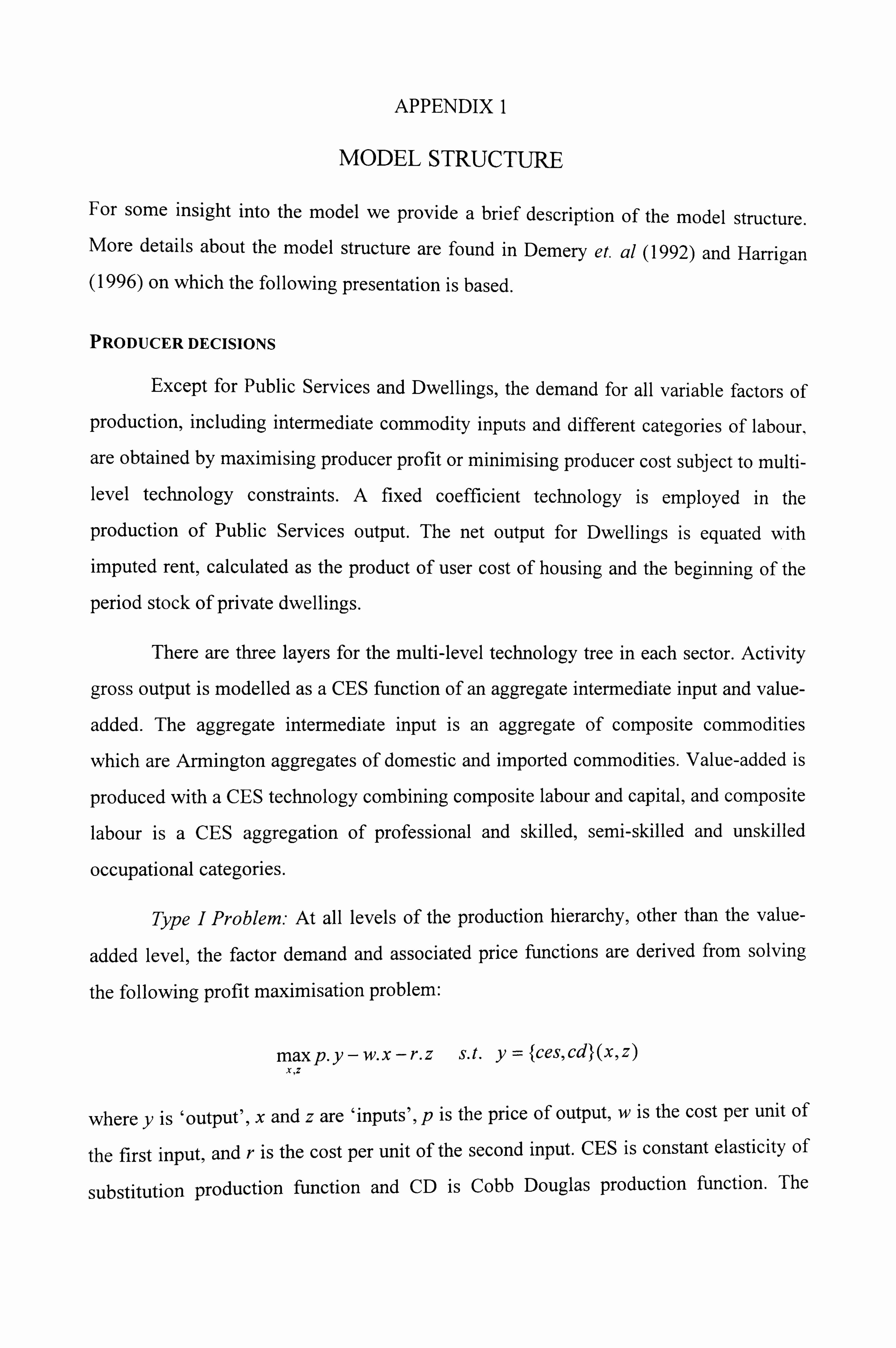
APPENDIX I

MODEL STRUCTURE

For some insight into the model we provide a brief description of the model structure. More details about the model structure are found in Demery et. al (1992) and Harrigan (1996) on which the following presentation is based.

PRODUCER DECISIONS

Except for Public Services and Dwellings, the demand for all variable factors of

production, including intermediate commodity inputs and different categories of labour,

are obtained by maximising producer profit or minimising producer cost subject to multi- level technology constraints. A fixed coefficient technology is employed in the

production of Public Services output. The net output for Dwellings is equated with imputed rent, calculated as the product of user cost of housing and the beginning of the

period stock of private dwellings.

There are three layers for the multi-level technology tree in each sector. Activity

gross output is modelled as a CES function of an aggregate intermediate input and value-

added. The aggregate intermediate input is an aggregate of composite commodities

which are Armington aggregates of domestic and imported commodities. Value-added is

produced with a CES technology combining composite labour and capital, and composite

labour is a CES aggregation of professional and skilled, semi-skilled and unskilled

occupational categories.

Type I Problem. - At all levels of the production hierarchy, other than the value-

added level, the factor demand and associated price functions are derived from solving

the following profit maximisation problem:

maxp. y-w. x-r. z s. t. y=fces, cdl(x, z) X, Z

where Y is 'output', x and z are 'inputs', p is the price of output, w is the cost per unit of

the first input, and r is the cost per unit of the second input. CES is constant elasticity of

substitution production function and CD is Cobb Douglas production function. The

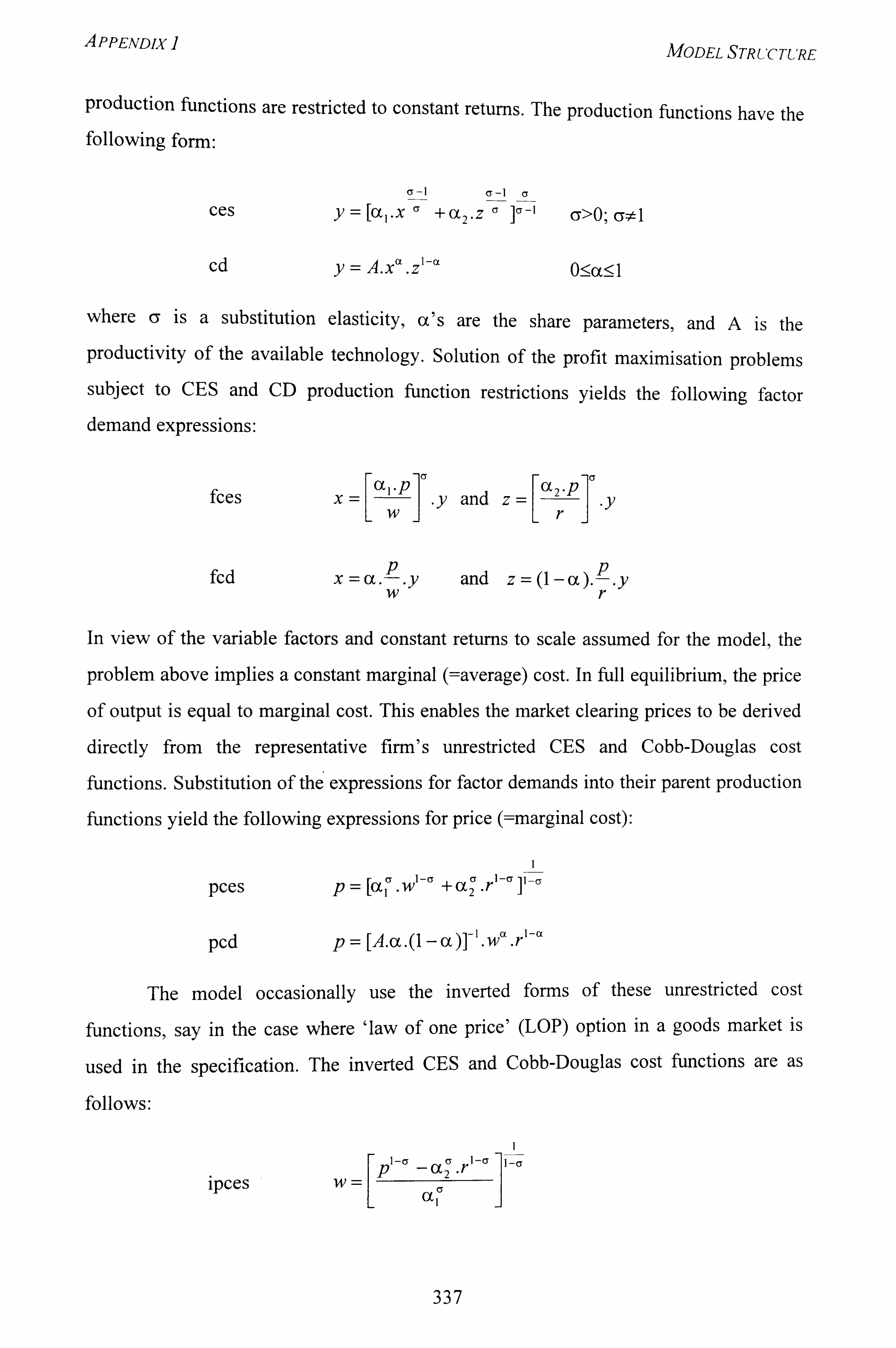
PPENDjx i MODEL STRUCTURE

production functions are restricted to constant returns. The production functions have the following form:

ces

cd

a -1 cr -I a [oC,. x a +(X

2'Z a la-I

A. x. zl-ct

G>O; cT# I

0:! kc< I

where cy is a substitution elasticity, cc's are the share parameters, and A is the

productivity of the available technology. Solution of the profit maximisation problems subject to CES and CD production function restrictions yields the following factor demand expressions:

cr a

(X2*P fces X= [(", P]

y and zI. y wr

fc dX =a. p

.. y and z -a). p.

y wr

In view of the variable factors and constant returns to scale assumed for the model, the

problem above implies a constant marginal (=average) cost. In full equilibrium, the price

of output is equal to marginal cost. This enables the market clearing prices to be derived

directly from the representative firm's unrestricted CES and Cobb-Douglas cost functions. Substitution of the expressions for factor demands into their parent production

functions yield the following expressions for price (=rnarginal cost):

1 1 -cy cr 1 1-G

pces p= lai w+ (X2 .r

pcd p= [A. a. (I - a)]-'. w'. r'-'

The model occasionally use the inverted forms of these unrestricted cost

functions, say in the case where 'law of one price' (LOP) option in a goods market is

used in the specification. The inverted CES and Cobb-Douglas cost functions are as

follows:

I I-a

oc2 r'-' I-cr

ipces p

CF 2

337

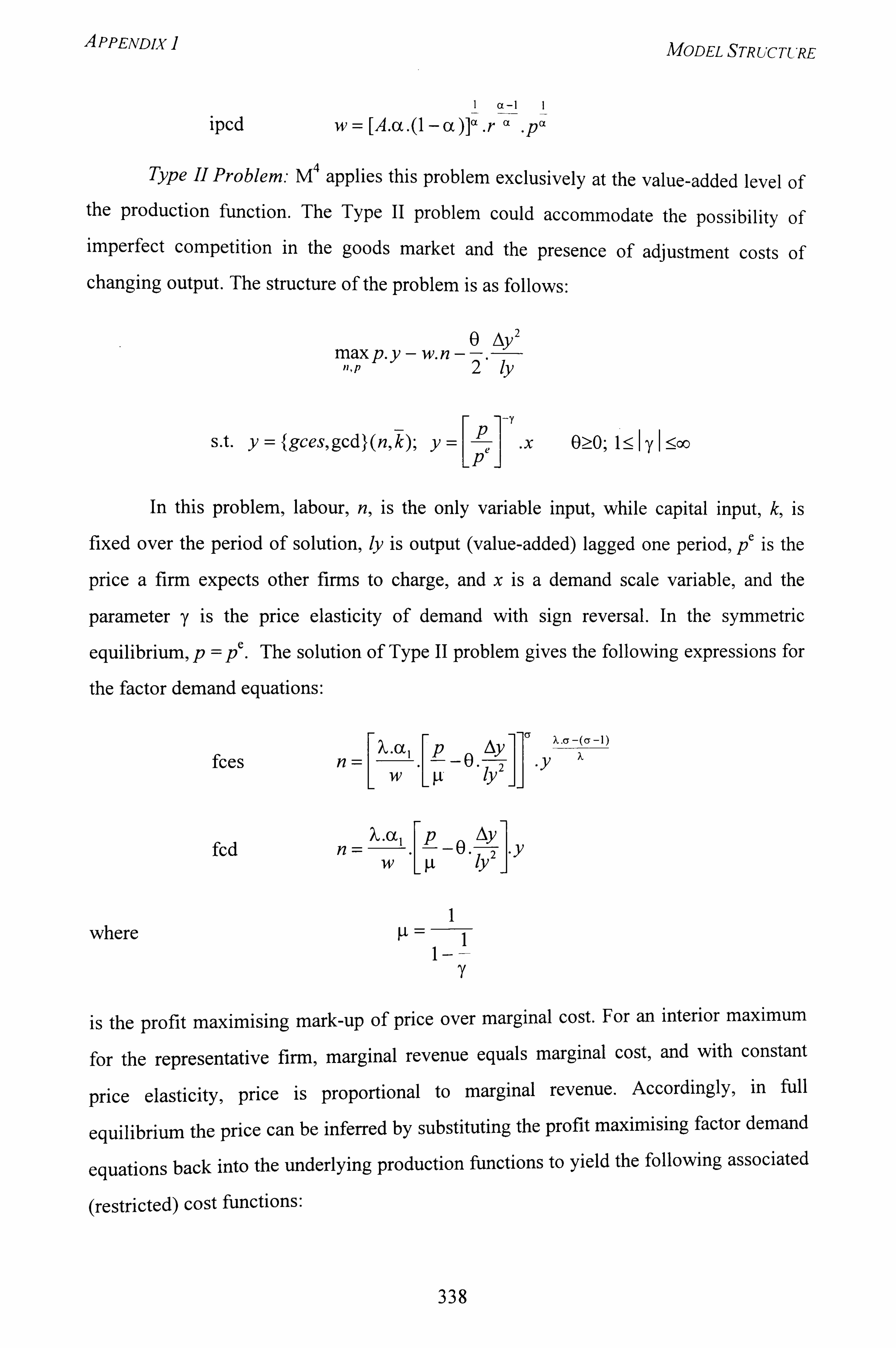
A PPENDIx I MODEL STRUCTURE

ipcd w= [A. (x. (l - u)]Ct. r Cc PCC C,

Type H Problem: M4 applies this problem exclusively at the value-added level of the production function. The Type 11 problem could accommodate the possibility of imperfect competition in the goods market and the presence of adjustment costs of

changing output. The structure of the problem is as follows:

maxp. y - w. n 0* Ay 2

11, p 2 ly

s. t. y=ý gces, gcd 1 (n, k); y=1P1-x Oýý0; i: ýý- 1y1: ýg00 e p

In this problem, labour, n, is the only variable input, while capital input, k, is

fixed over the period of solution, ly is output (value-added) lagged one period, p' is the

price a firm expects other firms to charge, and x is a demand scale variable, and the

parameter 7 is the price elasticity of demand with sign reversal. In the symmetric

e equilibrium, p=P. The solution of Type 11 problem gives the following expressions for

the factor demand equations:

cr ý'. a -(cr -1)

fces n AY

y 12 wy

fcd n= '-*(x'

.

[ýg -0-

Ay ]. y

ýt 12 wy

where 1

1 1---

is the profit maximising mark-up Of Price over marginal cost. For an interior maximum

for the representative firm, marginal revenue equals marginal cost, and with constant

price elasticity,, price is proportional to marginal revenue. Accordingly, in full

equilibrium the price can be inferred by substituting the profit maximising factor demand

equations back into the underlying production functions to yield the following associated

(restricted) cost functions:

338

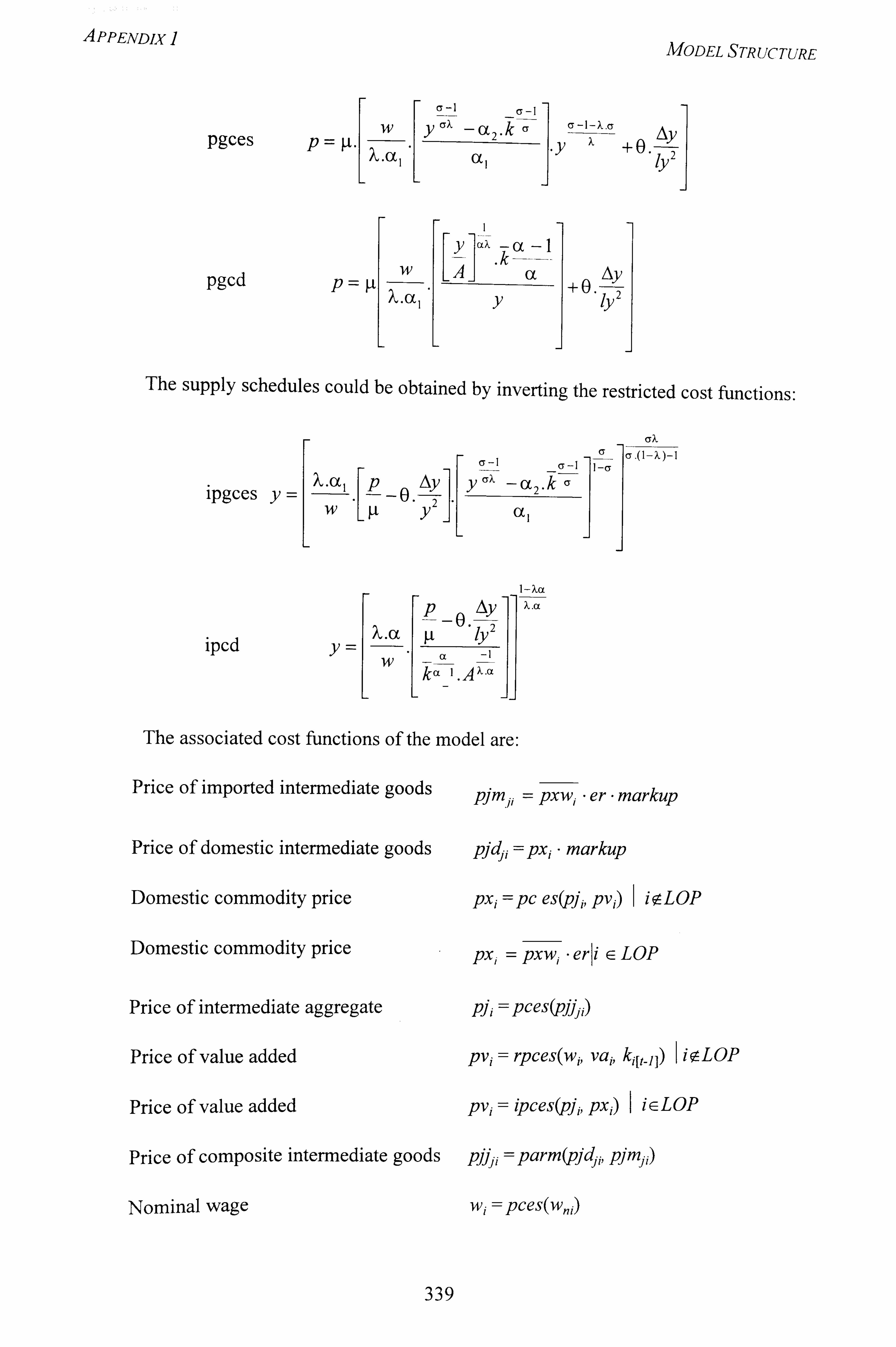
APPENDIX I MODEL STRUCTURE

y CC2 cr cr -1 pgces p --Z ýt- -x +0. AY

A-al (X] IY

[yl

uý. -(X -1 -. k

pgcd p= ýt wA U- AY

12 y

The supply schedules could be obtained by inverting the restricted cost ftinctions:

p Y, y (X 2 ipgces y2 y

L

I-X(x p

0. AY X. ct

9ý. (X g12 ipcd

(X y

w-- k(x-1. A1--01

The associated cost functions of the model are:

Price of imported intermediate goods pjm.,, = pxwi - er - markup

Price of domestic intermediate goods

Domestic commodity price

Domestic commodity price

Price of intermediate aggregate

Price of value added

Price of value added

Price of composite intermediate goods

Nominal wage

pjdji =pxi - markup

px, =pc es(pji, pvi) I ioLOP

px, = pxwi - erli E=- LOP

pji =pces(pjjji)

pvi = rpces(wi, vai, ki[t-, ]) I io-LOP

pvi = ipces(pji, pxi) I icLOP

pjj, i =parm(pjdji, pjmji)

wi = pces(w, j)

339

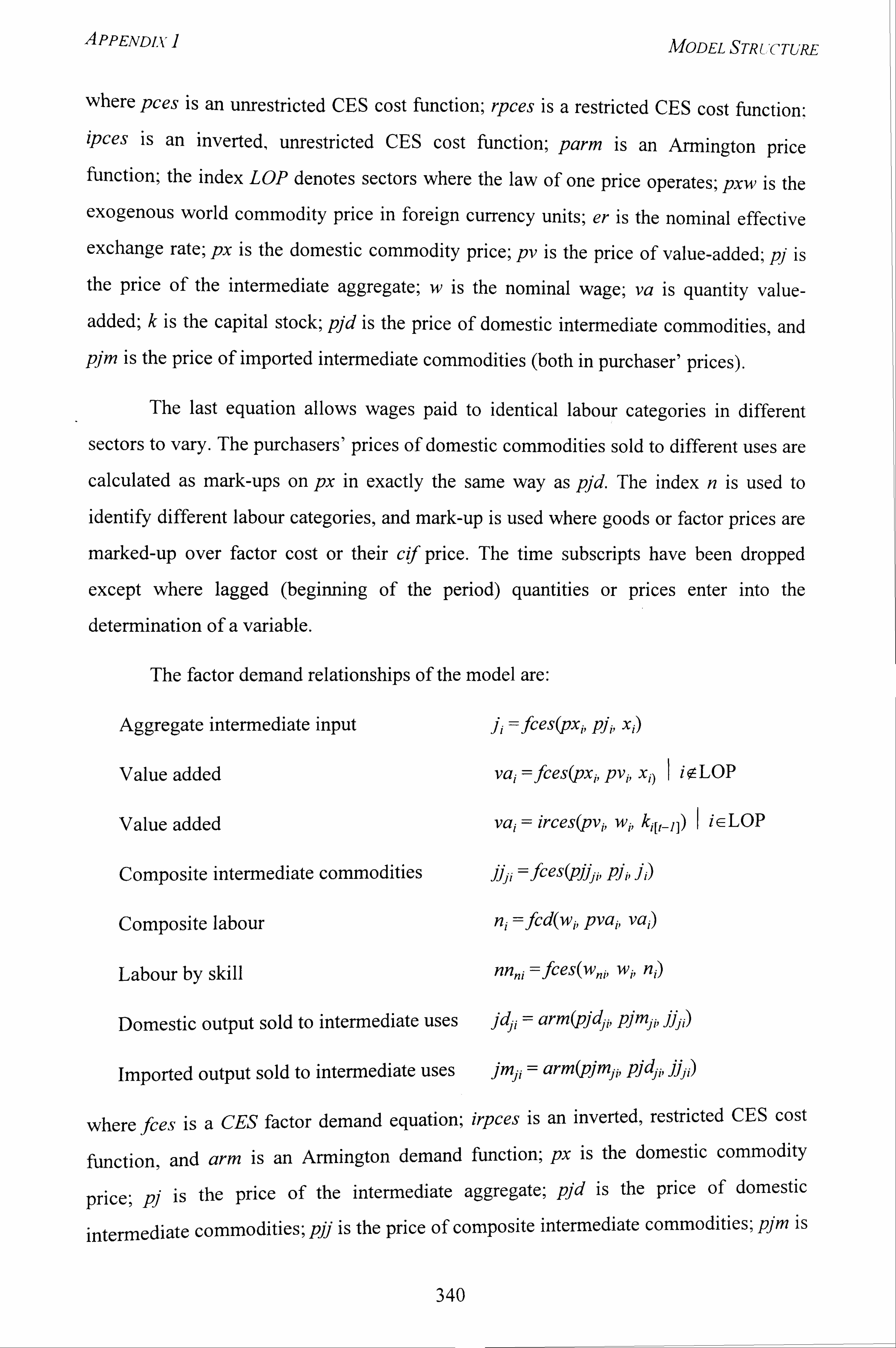
APPENDI. x- I MODEL STRUCTURE

where pces is an unrestricted CES cost function; rpces is a restricted CES cost function. ipces is an inverted, unrestricted CES cost function; parm is an Armington price function; the index LOP denotes sectors where the law of one price operates; pxw is the exogenous world commodity price in foreign currency units; er is the nominal effective exchange rate; px is the domestic commodity price; pv is the price of value-added; pj is

the price of the intermediate aggregate; w is the nominal wage; va is quantity value-

added; k is the capital stock; pjd is the price of domestic intermediate commodities, and

pjm is the price of imported intermediate commodities (both in purchaser' prices).

The last equation allows wages paid to identical labour categories in different

sectors to vary. The purchasers' prices of domestic commodities sold to different uses are

calculated as mark-ups on px in exactly the same way as pjd. The index n is used to

identify different labour categories, and mark-up is used where goods or factor prices are

marked-up over factor cost or their cif price. The time subscripts have been dropped

except where lagged (beginning of the period) quantities or prices enter into the

determination of a variable.

The factor demand relationships of the model are:

Aggregate intermediate input ji =fces(pxi, pji, xi)

Value added

Value added

Composite intermediate commodities

Composite labour

Labour by skill

Domestic output sold to intermediate uses

Imported output sold to intermediate uses

vai =ftes(pxi, pvi, xi) I io- LOP

vai = irces(pvi, wi, kip-1) I ic LOP

jý, j =fces(pjjj. i, pji, ji)

ni =ftd(wi, pvai, vai)

nnni : --fces(Wni, wi, ni)

jdji = arm(pjdji, pjmji, jj,. i)

jmj, = arm(pjmji, pidji, jj*j. i)

where fces is a CES factor demand equation; irpces is an inverted, restricted CES cost

function, and arm is an Armington demand function; px is the domestic commodity

price; pj is the price of the intermediate aggregate; pjd is the price of domestic

intermediate commodities; pjj is the price of composite intermediate commodities; pjm is

340

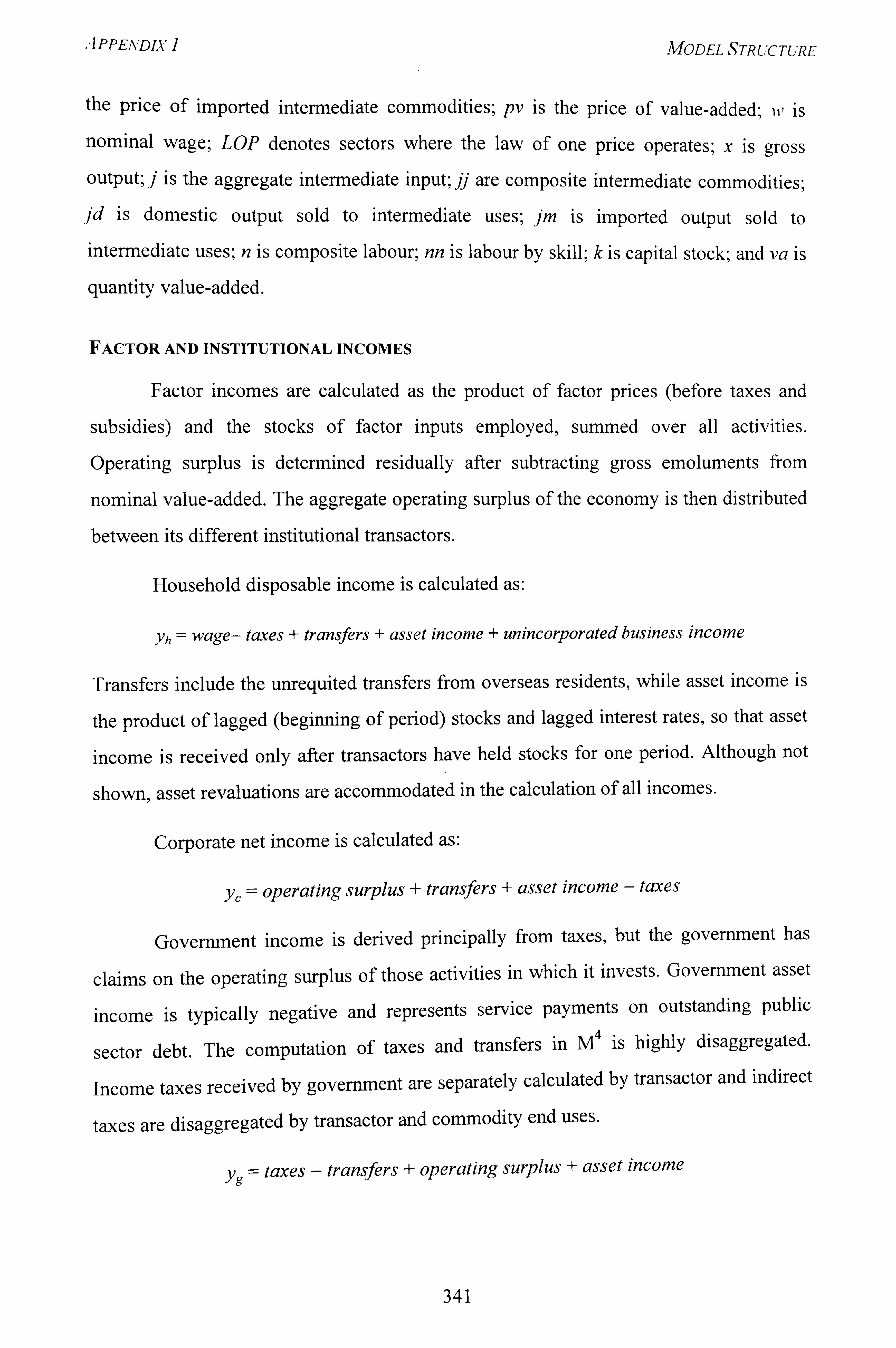
APPENDIX] MODEL STRUCTURE

the price of imported intermediate commodities; pv is the price of value-added; it, is

nominal wage; LOP denotes sectors where the law of one price operates; x is gross

output; j is the aggregate intermediate input; jj are composite intermediate commodities;

. jd is domestic output sold to intermediate uses; jm is imported output sold to intermediate uses; n is composite labour; nn is labour by skill; k is capital stock; and va is

quantity value-added.

FACTOR AND INSTITUTIONAL INCOMES

Factor incomes are calculated as the product of factor prices (before taxes and

subsidies) and the stocks of factor inputs employed, summed over all activities.

Operating surplus is determined residually after subtracting gross emoluments from

nominal value-added. The aggregate operating surplus of the economy is then distributed

between its different institutional transactors.

Household disposable income is calculated as:

Yh : -- wage- taxes + transfers + asset income + unincorporated business income

Transfers include the unrequited transfers from overseas residents, while asset income is

the product of lagged (beginning of period) stocks and lagged interest rates, so that asset

income is received only after transactors have held stocks for one period. Although not

shown, asset revaluations are accommodated in the calculation of all incomes.

Corporate net income is calculated as:

operating surplus + transfers + asset income - taxes

Government income is derived principally from taxes, but the government has

claims on the operating surplus of those activities in which it invests. Government asset

income is typically negative and represents service payments on outstanding public

sector debt. The computation of taxes and transfers in M4 is highly disaggregated.

Income taxes received by government are separately calculated by transactor and indirect

taxes are disaggregated by transactor and commodity end uses.

y9 == taxes - transfers + operating surplus + asset income

341

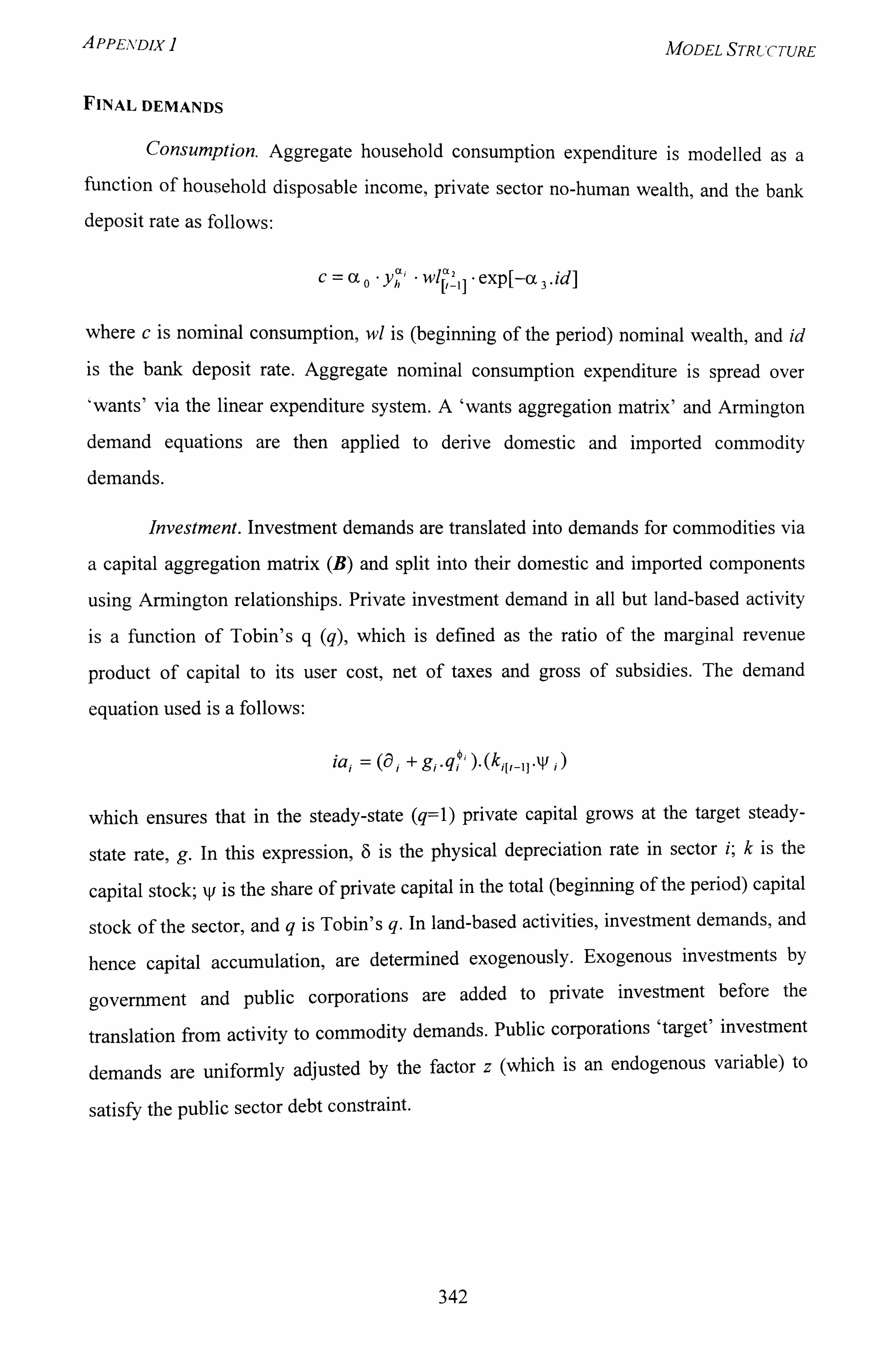
PPENDIX I

FINAL DEMANDS

MODEL STRUCTURE

Consumption. Aggregate household consumption expenditure is modelled as a function of household disposable income, private sector no-human wealth, and the bank deposit rate as follows:

ot 0. yoEi . WJGC2 /I [/-I] - expl-oý 3 Jd]

where c is nominal consumption, wl is (beginning of the period) nominal wealth, and id

is the bank deposit rate. Aggregate nominal consumption expenditure is spread over ýwants' via the linear expenditure system. A 'wants aggregation matrix' and Armington

demand equations are then applied to derive domestic and imported commodity demands.

Investment. Investment demands are translated into demands for commodities via

a capital aggregation matrix (B) and split into their domestic and imported components

using Armington relationships. Private investment demand in all but land-based activity

is a function of Tobin's q (q), which is defined as the ratio of the marginal revenue

product of capital to its user cost, net of taxes and gross of subsidies. The demand

equation used is a follows:

iai = (a, + g,. q, oi ). (kii, -, I. y j)

which ensures that in the steady-state (q=l) private capital grows at the target steady-

state rate, g. In this expression, 6 is the physical depreciation rate in sector i; k is the

capital stock; y is the share of private capital in the total (beginning of the period) capital

stock of the sector, and q is Tobin's q. In land-based activities, investment demands, and

hence capital accumulation, are determined exogenously. Exogenous investments by

government and public corporations are added to private investment before the

translation from activity to commodity demands. Public corporations 'target' investment

demands are uniformly adjusted by the factor z (which is an endogenous variable) to

satisfy the public sector debt constraint.

342

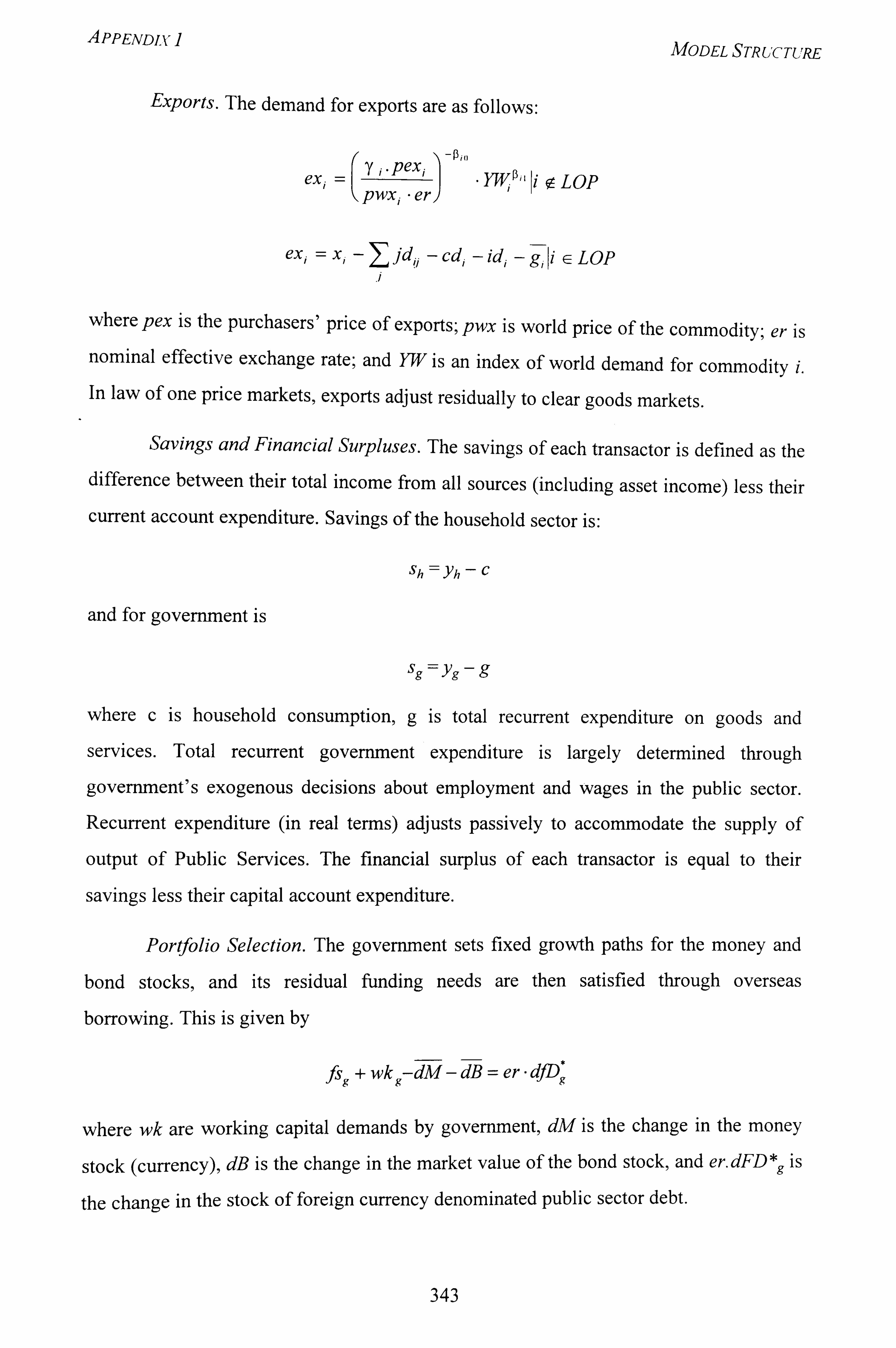
PPENDLV I

Exports. The demand for exports are as follows:

Pio

y i. pexi exi =

pwxi *er 2- YTýß" li « LOP

ex. = xi - jjd, - cd id -- Ii gi li EELOP

J

MODEL STRUCTURE

where pex is the purchasers' price of exports; pwx is world price of the commodity; er is nominal effective exchange rate; and YW is an index of world demand for commodity i. In law of one price markets, exports adjust residually to clear goods markets.

Savings and Financial Surpluses. The savings of each transactor is defined as the difference between their total income from all sources (including asset income) less their current account expenditure. Savings of the household sector is:

Sh ::::::::: Yh -C

and for government is

g : --Yg -9

where c is household consumption, g is total recurrent expenditure on goods and

services. Total recurrent government expenditure is largely determined through

government's exogenous decisions about employment and wages in the public sector. Recurrent expenditure (in real terms) adjusts passively to accommodate the supply of

output of Public Services. The financial surplus of each transactor is equal to their

savings less their capital account expenditure.

Poqfolio Selection. The government sets fixed growth paths for the money and

bond stocks, and its residual funding needs are then satisfied through overseas

borrowing. This is given by

fsg + wkg-dM - dB = er - d)Dg'

where wk are working capital demands by government, dM is the change in the money

stock (currency), dB is the change in the market value of the bond stock, and er. dFD*9 is

the change in the stock of foreign currency denominated public sector debt.

343

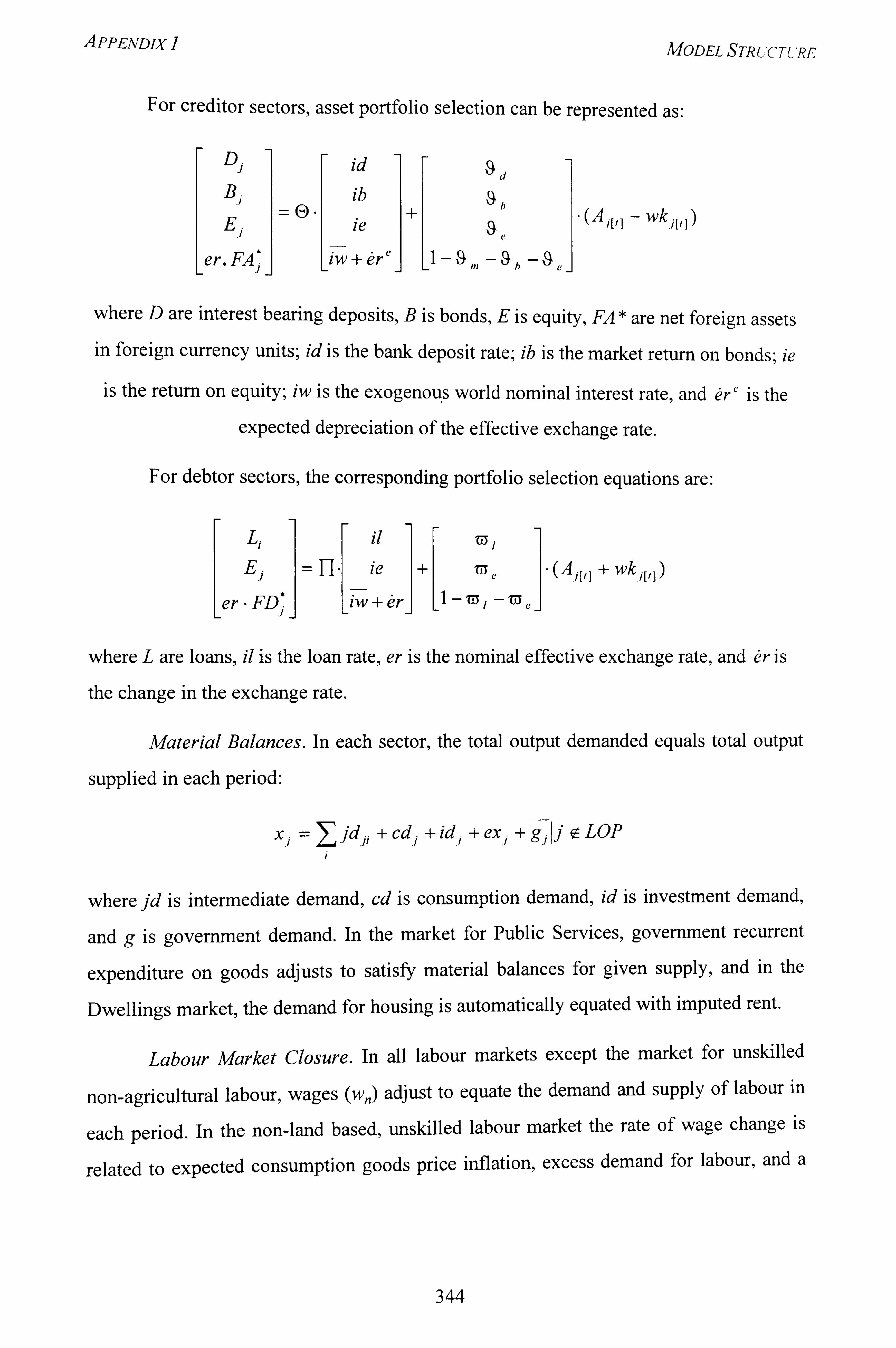
PPENDix I MODEL STRUCTURE

For creditor sectors, asset portfolio selection can be represented as:

Dj id Bi ib E ie

.i er. FA *

_iw +W

.i Ll

4 n)

wk

where D are interest bearing deposits, B is bonds, E is equity, FA * are net foreign assets in foreign currency units; id is the bank deposit rate; ib is the market return on bonds; ie

is the return on equity; iw is the exogenous world nominal interest rate, and ýr' is the

expected depreciation of the effective exchange rate.

For debtor sectors, the corresponding portfolio selection equations are:

Li

E ie

er - FD* iw+er

-(A + wk All

where L are loans, il is the loan rate, er is the nominal effective exchange rate, and ýr is

the change in the exchange rate.

Material Balances. In each sector, the total output demanded equals total output

supplied in each period:

x=+ cd + id + ex + gi Ij e- LOP jd. ji iii

where jd is intermediate demand, cd is consumption demand, id is investment demand,

and g is government demand. In the market for Public Services, government recurrent

expenditure on goods adjusts to satisfy material balances for given supply, and in the

Dwellings market, the demand for housing is automatically equated with imputed rent.

Labour Market Closure. In all labour markets except the market for unskilled

non-agricultural labour, wages (w,, ) adjust to equate the demand and supply of labour in

each period. In the non-land based, unskilled labour market the rate of wage change is

related to expected consumption goods price inflation, excess demand for labour, and a

344

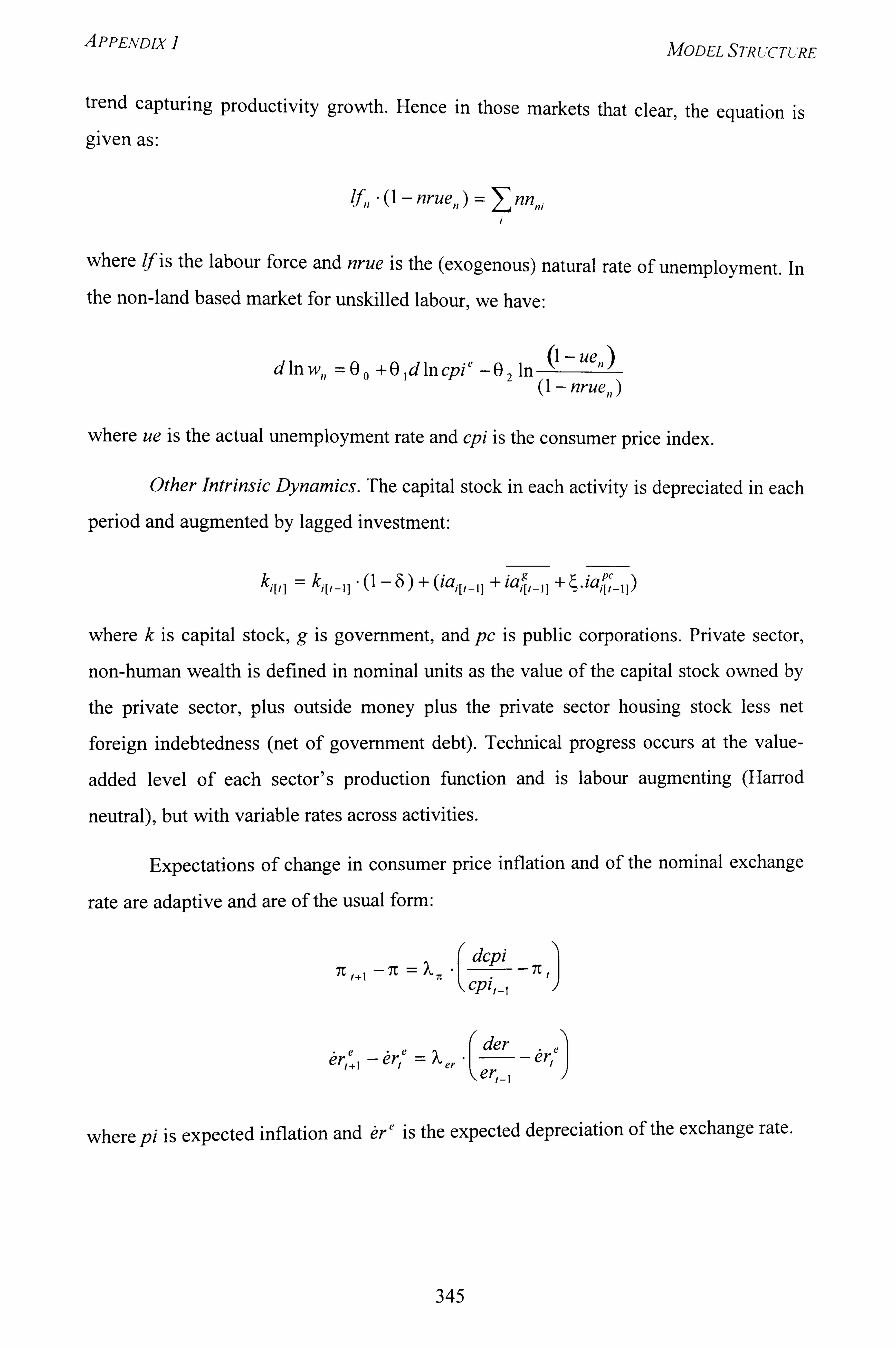
PPENDix I MODEL STRUCTURE

trend capturing productivity growth. Hence in those markets that clear, the equation is

given as:

nrue,, ) nn,

where 1f is the labour force and nrue is the (exogenous) natural rate of unemployment. In the non-land based market for unskilled labour, we have:

dlnw,, =00 +Odlncpi'-02 In - ue, )

nrue,, )

where ue is the actual unemployment rate and cpi is the consumer price index.

Other Intrinsic Dynamics. The capital stock in each activity is depreciated in each

period and augmented by lagged investment:

kil, l = kil, 6) + (iai[, + iag +4. ia'c ,) -11 ip-11 iti-

where k is capital stock, g is government, and pc is public corporations. Private sector,

non-human wealth is defined in nominal units as the value of the capital stock owned by

the private sector, plus outside money plus the private sector housing stock less net

foreign indebtedness (net of government debt). Technical progress occurs at the value-

added level of each sector's production function and is labour augmenting (Harrod

neutral), but with variable rates across activities.

Expectations of change in consumer price inflation and of the nominal exchange

rate are adaptive and are of the usual fonn:

7r /+I - 7t =k 7c -

(Cpit-l

- 7T I

der_ ýre ýr, '+, -

ýr, L : -- 7er '

er, -,

where pi is expected inflation and ýr' is the expected depreciation of the exchange rate.

345

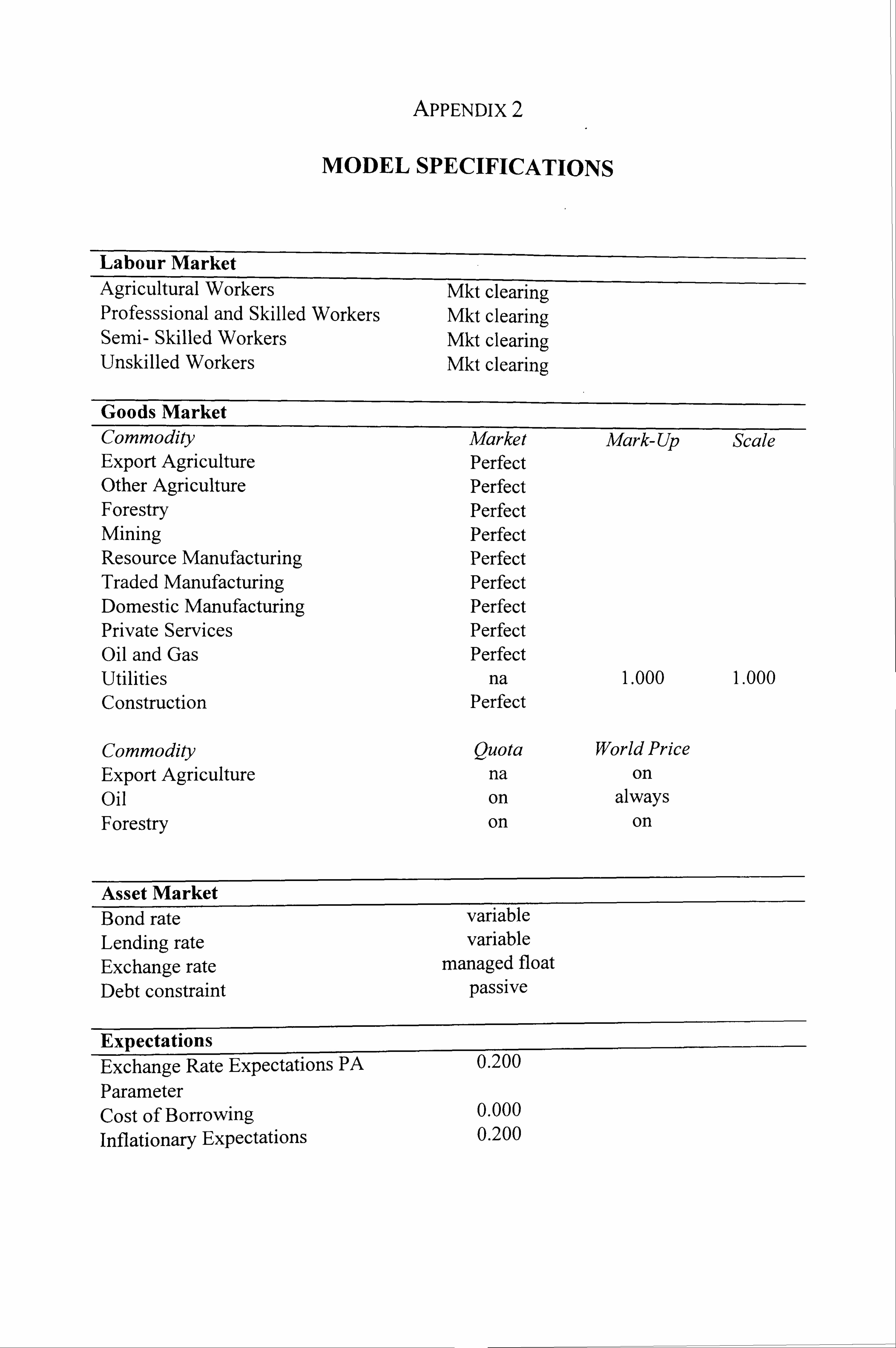
APPENDIX 2

MODEL SPECIFICATIONS

Labour Market Agricultural Workers Mkt clearing Professsional and Skilled Workers Mkt clearing Serni- Skilled Workers Mkt clearing Unskilled Workers Mkt clearing

Goods Market Commodity Market Mark- Up Scale Export Agriculture Perfect Other Agriculture Perfect Forestry Perfect Mining Perfect Resource Manufacturing Perfect Traded Manufacturing Perfect Domestic Manufacturing Perfect Private Services Perfect Oil and Gas Perfect Utilities na 1.000 1.000 Construction Perfect

Commodity Quota World Price Export Agriculture na on Oil on always Forestry on on

Asset Market Bond rate variable Lending rate variable Exchange rate managed float Debt constraint passive

Expectations Exchange Rate Expectations PA 0.200 Parameter Cost of Borrowing 0.000

Inflationary Expectations 0.200

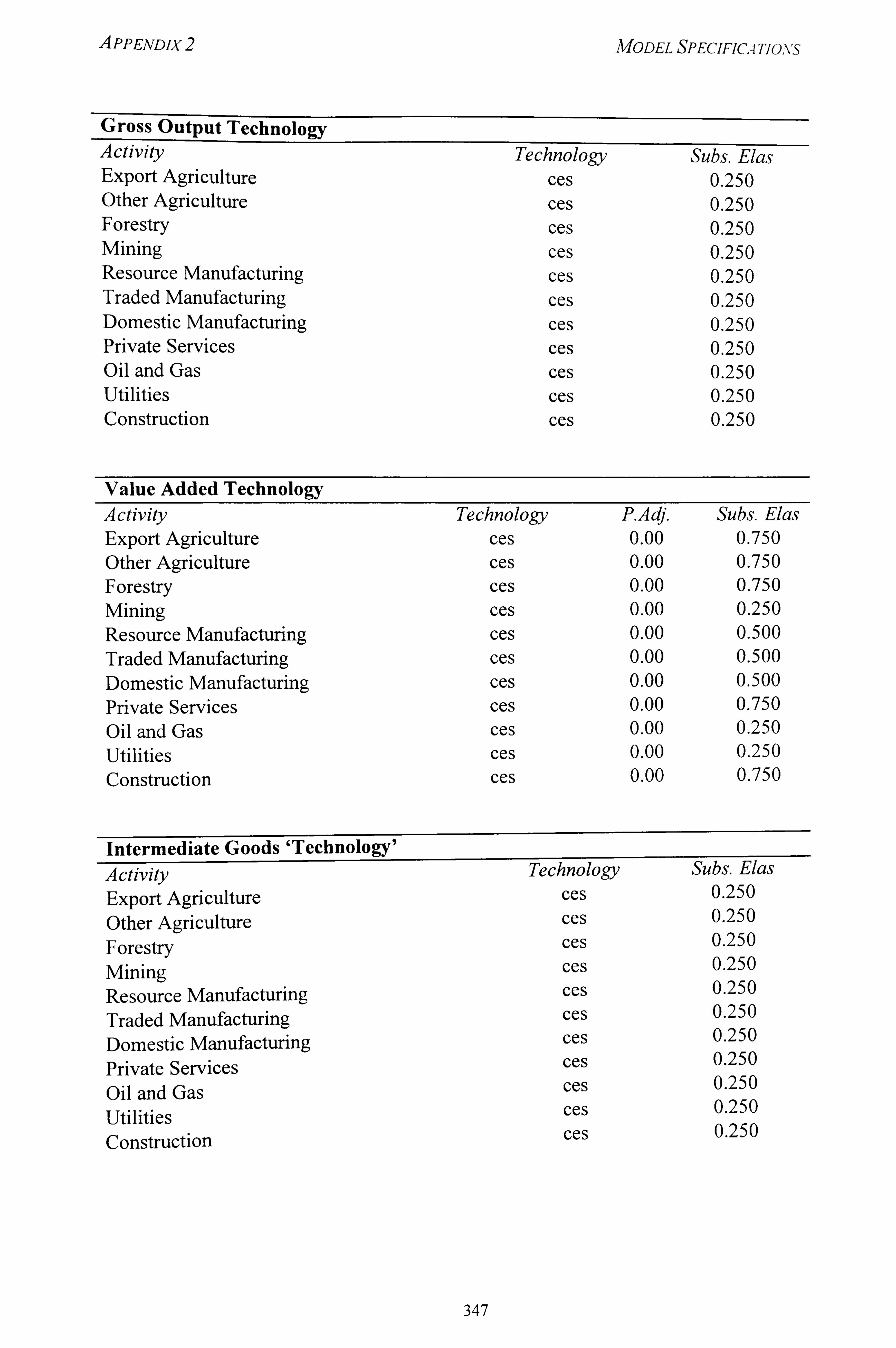
PPENDIX 2 MODEL SPECIFIC-1 Tjo, vS

Gross Output Technology Activity Technology Subs. Elas Export Agriculture ces 0.250 Other Agriculture ces 0.250 Forestry ces 0.250 Mining ces 0.250 Resource Manufacturing ces 0.250 Traded Manufacturing ces 0.250 Domestic Manufacturing ces 0.250 Private Services ces 0.250 Oil and Gas ces 0.250 Utilities ces 0.250 Construction ces 0.250

Value Added Technology Activity Technology P. Adj. Subs. Elas Export Agriculture ces 0.00 0.750 Other Agriculture ces 0.00 0.750 Forestry ces 0.00 0.750 Mining ces 0.00 0.250 Resource Manufacturing ces 0.00 0.500 Traded Manufacturing ces 0.00 0.500 Domestic Manufacturing ces 0.00 0.500 Private Services ces 0.00 0.750 Oil and Gas ces 0.00 0.250 Utilities ces 0.00 0.250 Construction ces 0.00 0.750

Intermediate Goods 'Technology' Activity Technology Subs. Elas

Export Agriculture ces 0.250

Other Agriculture ces 0.250

Forestry ces 0.250

Mining ces 0.250

Resource Manufacturing ces 0.250

Traded Manufacturing ces 0.250

Domestic Manufacturing ces 0.250

Private Services ces 0.250

Oil and Gas ces 0.250

Utilities ces 0.250

Construction ces 0.250

347

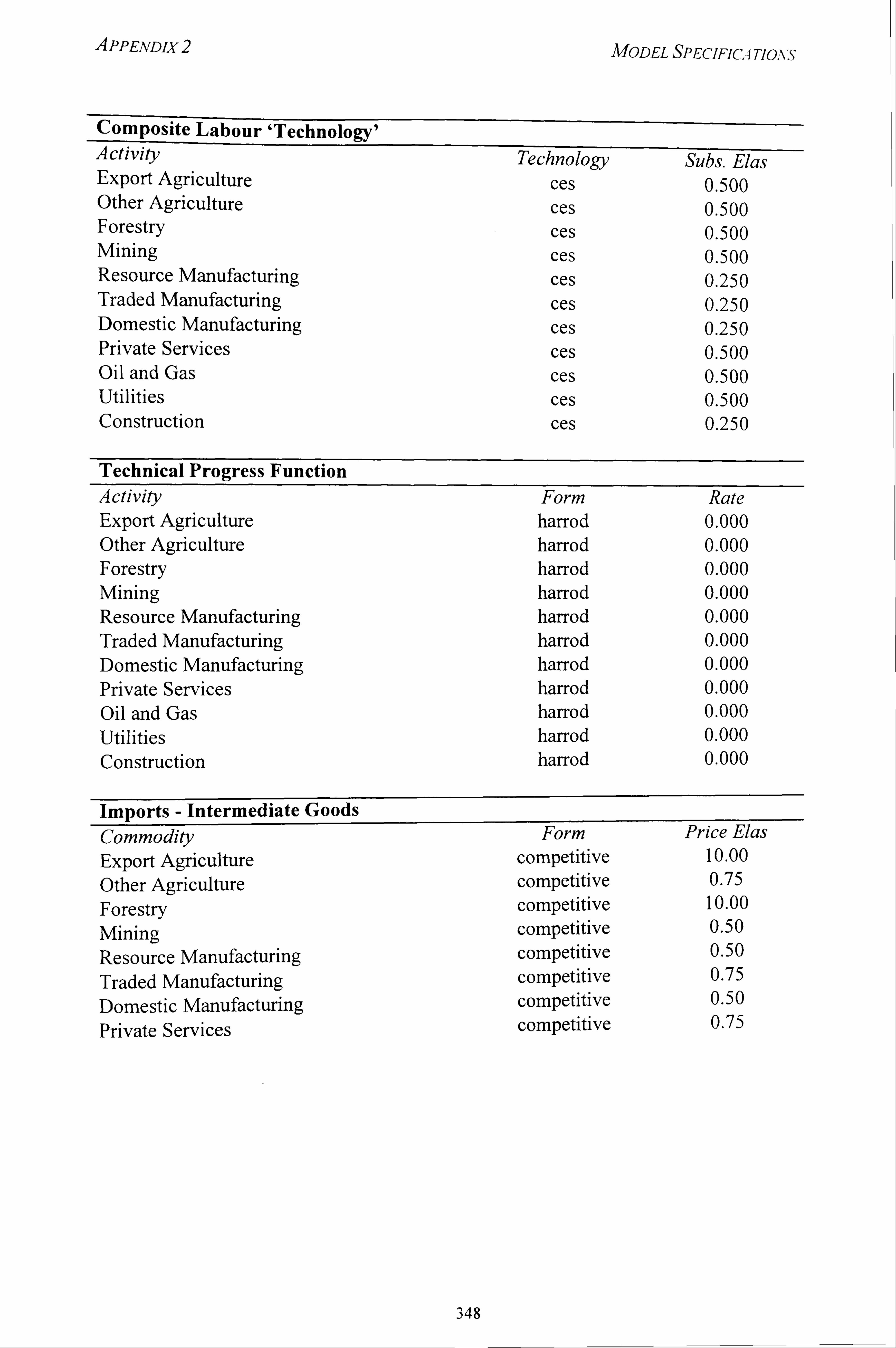
A PPENDIX 2 MODEL SPECIFICA TIONS

Composite Labour 'Technology' A ctivity Technology Subs. Elas Export Agriculture ces 0.500 Other Agriculture ces 0.500 Forestry ces 0.500 Mining ces 0.500 Resource Manufacturing ces 0.250 Traded Manufacturing ces 0.250 Domestic Manufacturing ces 0.250 Private Services ces 0.500 Oil and Gas ces 0.500 Utilities ces 0.500 Construction ces 0.250

Technical Progress Function Activity Form Rate Export Agriculture harrod 0.000 Other Agriculture harrod 0.000 Forestry harrod 0.000 Mining harrod 0.000 Resource Manufacturing harrod 0.000 Traded Manufacturing harrod 0.000 Domestic Manufacturing harrod 0.000 Private Services harrod 0.000 Oil and Gas harrod 0.000 Utilities harrod 0.000 Construction harrod 0.000

Imports - Intermediate Goods Commodity Form Price Elas Export Agriculture competitive 10.00 Other Agriculture competitive 0.75

Forestry competitive 10.00

Mining competitive 0.50

Resource Manufacturing competitive 0.50

Traded Manufacturing competitive 0.75

Domestic Manufacturing competitive 0.50

Private Services competitive 0.75

348

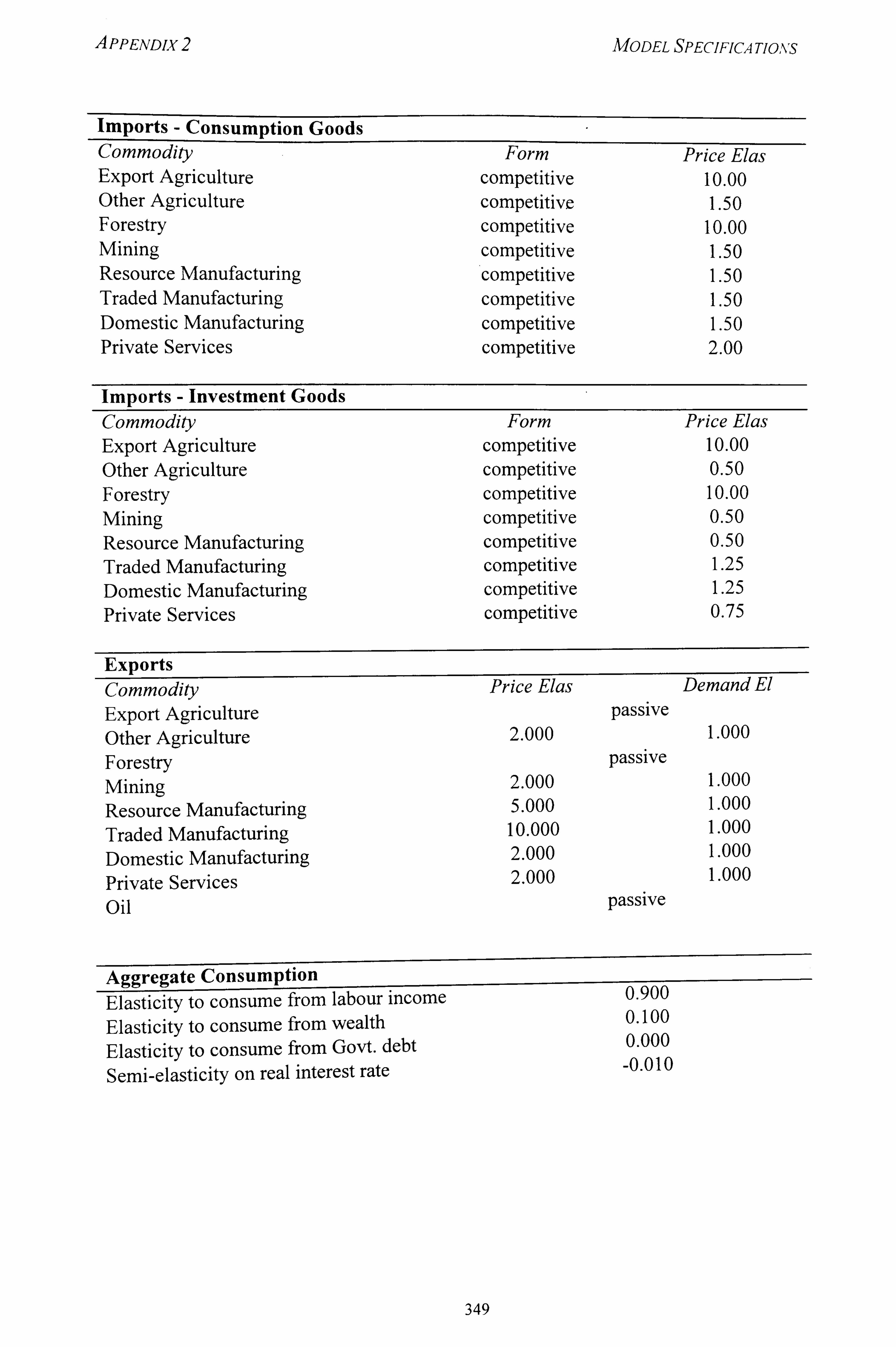
A PPENDLV 2 MODEL SPECIFICA TIONS

Imports - Consumption Goods Commodity Form Price Elas Export Agriculture competitive 10.00 Other Agriculture competitive 1.50 Forestry competitive 10.00 Mining competitive 1.50 Resource Manufacturing competitive 1.50 Traded Manufacturing competitive 1.50 Domestic Manufacturing competitive 1.50 Private Services competitive 2.00

Imports - Investment Goods Commodity Form Price Elas Export Agriculture competitive 10.00 Other Agriculture competitive 0.50 Forestry competitive 10.00 Mining competitive 0.50 Resource Manufacturing competitive 0.50 Traded Manufacturing competitive 1.25 Domestic Manufacturing competitive 1.25 Private Services competitive 0.75

Exports Commodity Price Elas Demand El

Export Agriculture passive Other Agriculture 2.000 1.000

Forestry passive Mining 2.000 1.000

Resource Manufacturing 5.000 1.000

Traded Manufacturing 10.000 1.000

Domestic Manufacturing 2.000 1.000

Private Services 2.000 1.000

Oil passive

Aggregate Consumption Elasticity to consume from labour income 0.900

Elasticity to consume from wealth 0.100

Elasticity to consume from Govt. debt 0.000

Semi-elasticity on real interest rate -0.010

349

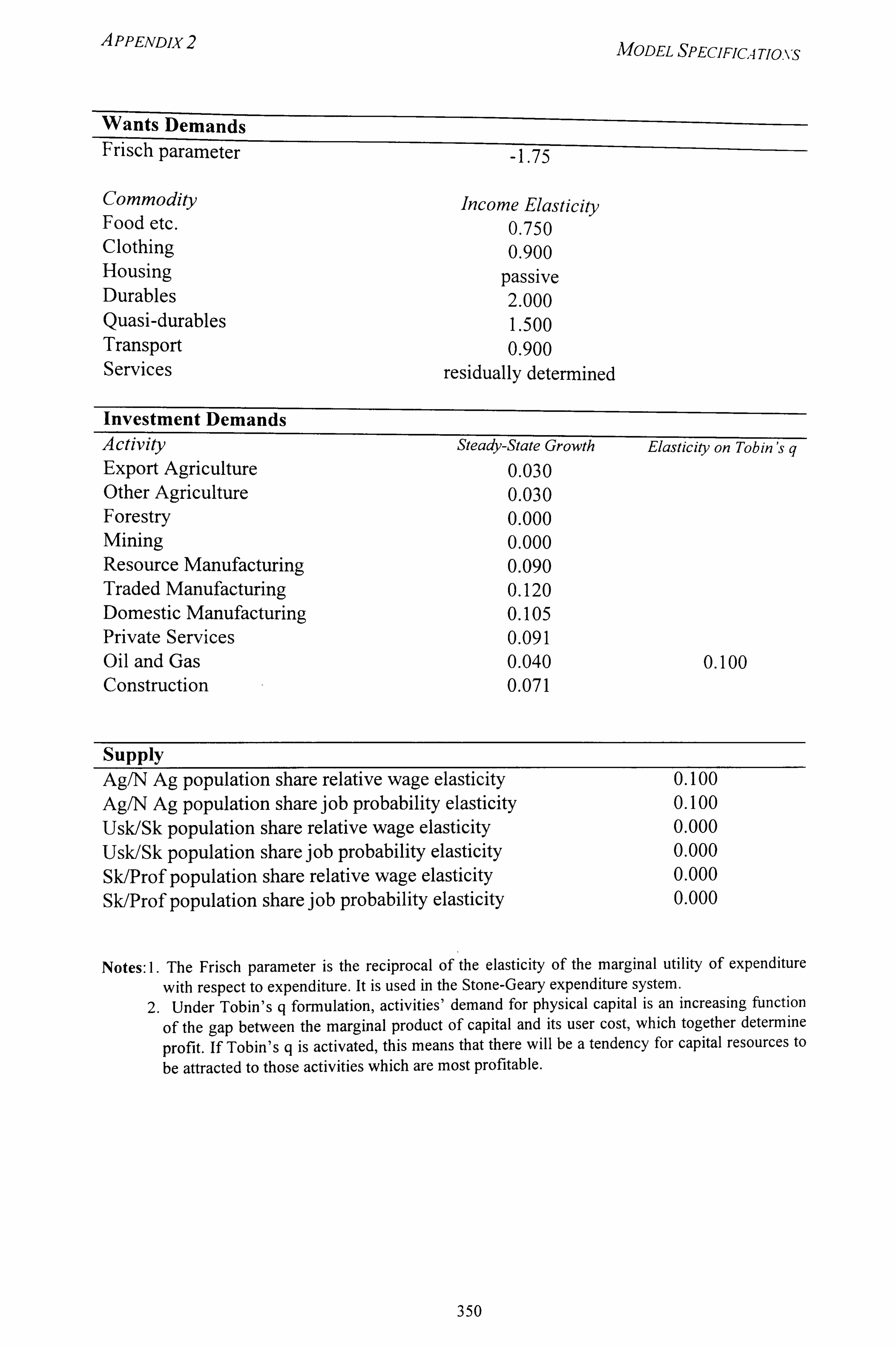
PPENDIX MODEL SPECIFIC4 TIOAS

Wants Demands Frisch parameter -1.75

Commodity Food etc. Clothing Housing Durables Quasi-durables Transport Services

Income Elasticity 0.750 0.900

passive 2.000 1.500 0.900

residually determined

Investment Demands Activity Steady-State Growth Export Agriculture 0.030 Other Agriculture 0.030 Forestry 0.000 Mining 0.000 Resource Manufacturing 0.090 Traded Manufacturing 0.120 Domestic Manufacturing 0.105 Private Services 0.091 Oil and Gas 0.040 Construction 0.071

Supply

Elasticity on Tobin's q

0.100

Ag/N Ag population share relative wage elasticity 0.100 Ag/N Ag population share job probability elasticity 0.100 Usk/Sk population share relative wage elasticity 0.000 Usk/Sk population share job probability elasticity 0.000 Sk/Prof population share relative wage elasticity 0.000 Sk/Prof population share job probability elasticity 0.000

Notes: 1. The Frisch parameter is the reciprocal of the elasticity of the marginal utility of expenditure with respect to expenditure. It is used in the Stone-Geary expenditure system.

2. Under Tobin's q fonnulation, activities' demand for physical capital is an increasing function

of the gap between the marginal product of capital and its user cost, which together determine

profit. If Tobin's q is activated, this means that there will be a tendency for capital resources to be attracted to those activities which are most profitable.

350

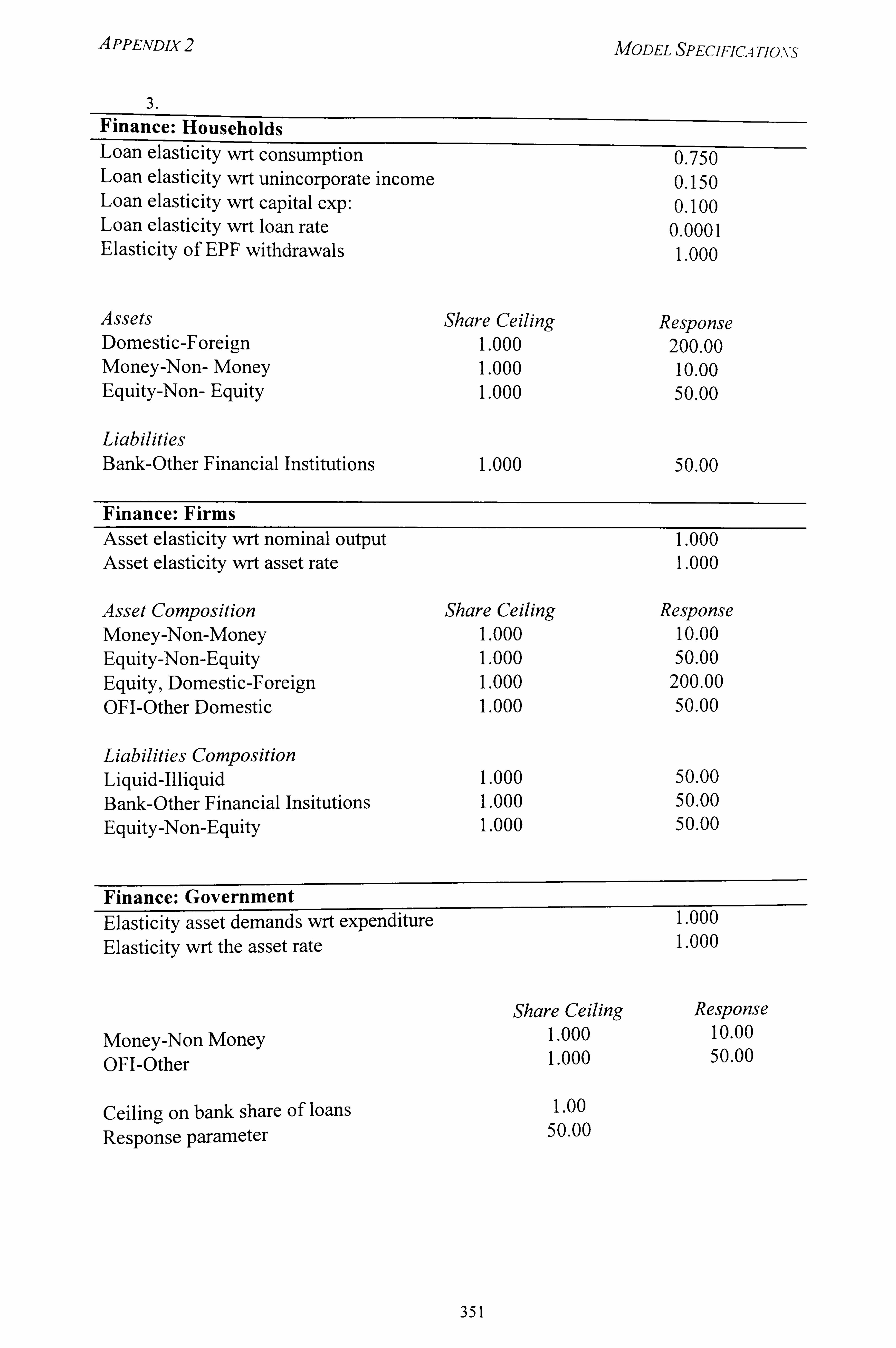
PPENDIX

3.

MODEL SPECIFICA TJOA'S

Finance: Households Loan elasticity wrt consumption 0.750 Loan elasticity wrt unincorporate income 0.150 Loan elasticity wrt capital exp: 0.100 Loan elasticity wrt loan rate 0.0001 Elasticity of EPF withdrawals 1.000

Assets Dome stic-F oreign Money-Non- Money Equity-Non- Equity

Liabilities Bank-Other Financial Institutions

Share Ceiling Response 1.000 200.00 1.000 10.00 1.000 50.00

1.000 50.00

Finance: Firms Asset elasticity wrt nominal output Asset elasticity wrt asset rate

Asset Composition Money-Non-Money Equity-Non-Equity Equity, Domestic-Foreign OFI-Other Domestic

Liabilities Composition Liquid-Illiquid Bank-Other Financial Insitutions Equity-Non-Equity

1.000 1.000

Share Ceiling Response 1.000 10.00 1.000 50.00 1.000 200.00 1.000 50.00

1.000 50.00 1.000 50.00 1.000 50.00

Finance: Government Elasticity asset demands wrt expenditure Elasticity wrt the asset rate

Share Ceiling

Money-Non Money 1.000

OFI-Other 1.000

Ceiling on bank share of loans 1.00 Response parameter 50.00

1.000 1.000

Response 10.00 50.00

351

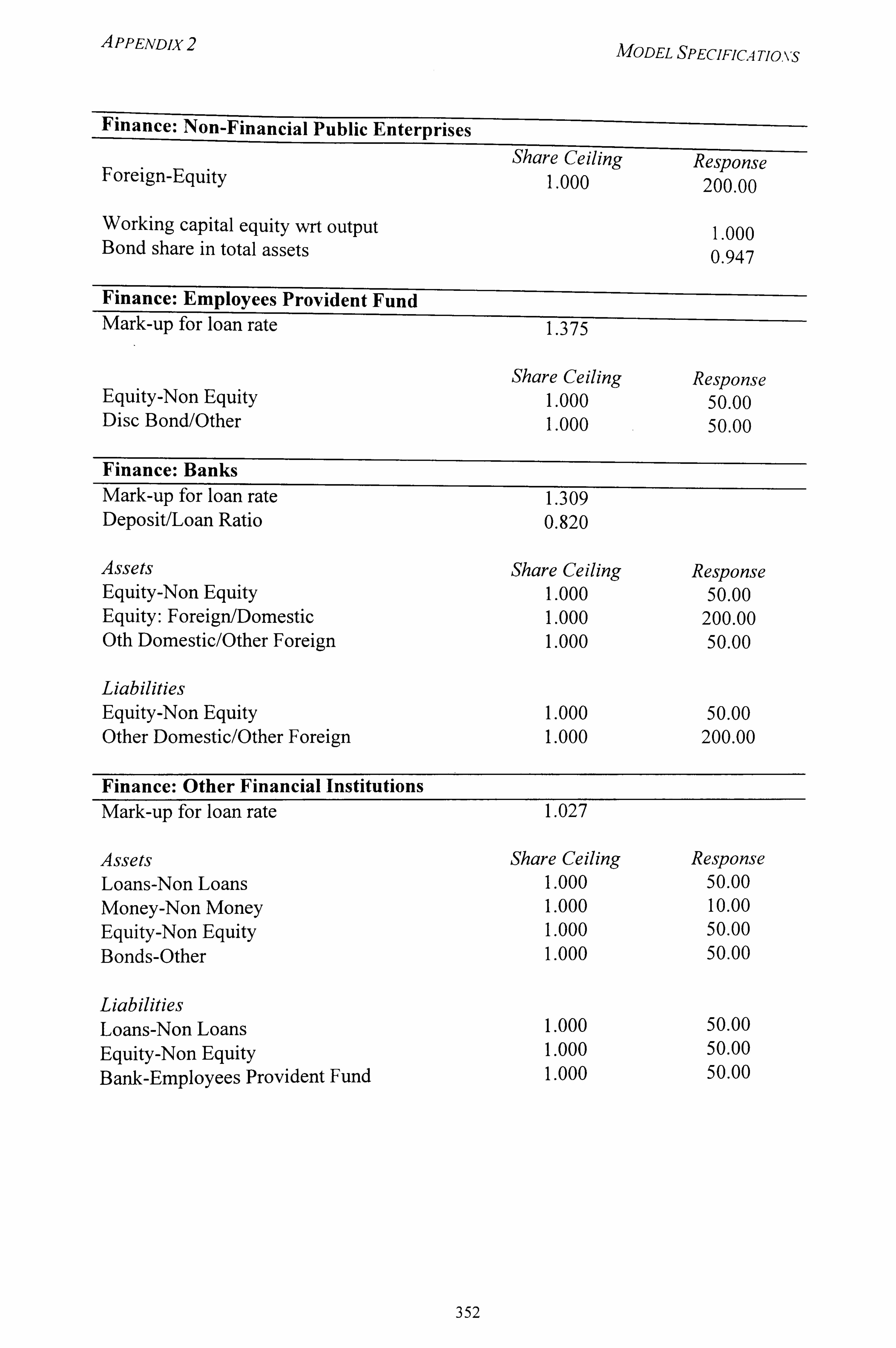
APPENDIX2 MODEL SPECIFICA TIO, VS

Finance: Non-Financial Public Enterprises Share Ceiling Response

Foreign-Equity 1.000 200.00

Working capital equity wrt output 1.000 Bond share in total assets 0.947

Finance: Employees Provident Fund Mark-up for loan rate 1.375

Share Ceiling Response Equity-Non Equity 1.000 50.00 Disc Bond/Other 1.000 50.00

Finance: Banks Mark-up for loan rate 1.309 Deposit/Loan Ratio 0.820

Assets Share Ceiling Response Equity-Non Equity 1.000 50.00 Equity: Foreign/Domestic 1.000 200.00 Oth Domestic/Other Foreign 1.000 50.00

Liabilities Equity-Non Equity 1.000 50.00 Other Domestic/Other Foreign 1.000 200.00

Finance: Other Financial Institutions Mark-up for loan rate 1.027

Assets Loans-Non Loans Money-Non Money Equity-Non Equity Bonds-Other

Liabilities Loans-Non Loans Equity-Non Equity Bank-Employees Provident Fund

Share Ceiling Response 1.000 50.00 1.000 10.00 1.000 50.00 1.000 50.00

1.000 50.00 1.000 50.00 1.000 50.00

352

BIBLIOGRAPHY

Adelman, L and S. Robinson. 1978. Income Distribution Policy in Developing Countries. - A Case Study of Korea. Stanford, CA: Stanford University Press.

Ahmad, S. E. and N. H. Stem. 1984. The Theory of Reforrn and Indian Indirect Taxes, Journal ofPublic Economics, 25: 259-295.

Ahmad, S. E. and N. H. Stem. 1986. Tax Reform for Pakistan: Overview and Effective Taxes for 1975/76,, Pakistan Development Review, Spring: 43-72.

Ahmad, S. E. and N. H. Stem. 1987. Alternative Sources of Government Revenue: Illustrations from India for 1979/80, in D. M. G. Newbery and N. H. Stern, eds., The Theory of Taxation for Developing Countries. New York: Oxford University

Press and World Bank.

Ahmad, S. E. and N. H. Stem. 1989. Taxation for Developing Countries, in H. Chenery

and T. N. Srinivasan, Handbook of Development Economics, vol. 11. North-

Holland: Elsevier Science Publishers B. V.

Ahmad,, E. and N. H Stem. 199 1. The Theory and Practice of Tax Reform in Developing

Countries. Cambridge University Press.

Ariff, M. 199 1. The Malaysian Economy: Pacific Connections. Oxford University Press.

Ashenfelter, 0., and J. J. Heckman. 1973. Estimating Labor Supply Functions, in Cain

and Watts, eds. 1973,265-78.

Asher, M. G. and A. Booth. 1983. Indirect Taxation In ASEAN, Singapore University

Press.

Ashworth, J. A. and D. T. Ulph. 1981. Estimating Labor Supply with Piecewise Linear

Budget Constraints, in C. Brown, ed., Taxation and Labor Supply. London.

Atkinson, A. B., and J. E. Stiglitz. 1980. Lecture on Pubic Economics. Singapore:

McGraw Hill, International Edition.

Azhar, B. A. and S. M. Sharif. 1974. The Effects of Tax Holiday on Investment Decisions:

An Empirical Analysis, Pakistan Development Review 13: 409-32.

BIBLIOGRAPHY

Bagchi, A. and M. Govinda Rao. 1982. Elasticity of Non-Corporate Tax in India, Economic and Political Weekly, 17: 1452-58.

Bahl, R. 1989. The Political Economy of the Jamaican Tax Reform,, in M. Gillis (ed. ) Tax Reform in Developing Countries. Durham: Duke University Press, 115-176.

Bahl, R. W. 1971. A Regression Approach to Tax Effort and Tax Ratio Analysis, IMF

Staff Papers, 18: 5 70-612.

Bahl, R. W. 1989. The Political Economy of the Jamaican Tax Reform, in Gillis,, 1989,,

115-176.

Ballard, C. L., D. Fullerton, J. B. Shoven, and J. Whalley. 1985. A General Equilibrium

Model For Tax Policy Evaluation. Chicago: University of Chicago Press.

Ballard, C. L., J. B. Shoven, J. Whalley. 1985. General Equilibrium Computation of the

Marginal Welfare Costs of U. S. Taxes. American Economic Review, 1985.

Ballentine, J. G. and W. Thirsk. 1979. The Fiscal Incidence of Some Experiments in

Fiscal Federalism. Ottawa: Canadian Mortgage and Housing Corporation.

Bank Negara Malaysia. Annual Report. Kuala Lumpur, various years.

Bardai, B. 1993. Malaysian Tax Policy: Applied General Equilibrium Analysis. Petaling

Jaya, Malaysia: Pelanduk Publications.

Bardhan, P. K. 1979. Labor Supply Functions in a Poor Agrarian Economy. American

Economic Review. Vol. 69,73-83.

Bardhan, P. K. 1984. Determinants of Supply and Demand of Labor in a Poor Agrarian

Economy: An Analysis of Household Survey Data from Rural West Bengal, in

H. P. Binswanger and M. R. Rosenzweig (eds. ) Contractual Arrangements,

Employment, and Wages in Rural Labor Markets in Asia. New Haven: Yale

University Press.

Barlow, R., H. Brazer and J. Morgan. 1966. Economic Behavior of the Affluent.

Washington, D. C.

Bartlett, B. R. 1982. Reaganomics. - Supply Side Economics in Action. New York: Quill,

updated.

354

BIBLIOGRAPHY

Bauer,, P. T. 1957. Economic Analysis and Policy in Underdeveloped Countries. Durham: Duke University Press.

Bauer, P. T. and B. S. Yarney. 1957. The Economics of Under-Developed Countries. Chicago: University of Chicago Press.

Becker, G. S. 1964. Human Capital. Second Edition. Columbia University Press.

Bender, B. 1989. A Simple General Equilibrium Analysis of the Relationship Between Real Tax Revenue and the Tax Rate. Scottish Journal of Political Economy, Vol. 36, No. 4,321-333.

Berg, E. J. 1961. Backward- Sloping Labor Supply Functions in Dual Economies: The

Africa Case. Quarterly Journal of Economics. Cambridge, Mass., Vol. 75,468- 492.

Bergman, L. 1990. The Development of Computable General Equilibrium Modeling, in

L. Bergman, D. W. Jorgenson, and E. Zalai, eds., General Equilibrium Modeling

and Economic Policy Analysis. Cambridge, Mass: Basil Blackwell.

Bilsborrow, R. E. and R. C. Porter. 1972. The Effects of Tax Exemption on Investment by

Industrial Firms in Colombia, Weltwirstschaftliches Archiv 108: 396-425.

Bird, R. M and 0. Oldman. 1990. Taxation in Developing Countries. Fourth Edition.

Baltimore and London: Johns Hopkins University Press.

Bird, R. M. 1989. The Administrative Dimension of Tax Reform in Developing

Countries, in M. Gillis, ed. Tax Reform in Developing Countries, 315-46.

Durham, N. C.: Duke University Press.

Bloch, F. 1973. The Allocation of Time to Market and Nonmarket Work Within a

Family Unit. Technical Report No. 114, Institute for Mathematical Studies in the

Social Sciences, Stanford University.

Blomquist, S. 1983. The Effect of Income Taxation on the Labor Supply of Married Men

in Sweden. Journal ofPublic Economics 22,169-197.

Blomquist, S. 1996. Estimation Methods for Male Labor Supply Functions: How to Take

Account of Nonlinear Taxes. Journal of Econometrics 70,383-405.

355

BIBLIOGRAPHY

Blundell, R. W. 1980. Estimating Continuous Consumer Equivalence Scales in an Expenditure Model With Labour Supply. European Economic Review 14 (1980), 145-157.

Blundell, R. W.,, C. Meghir, E. Symons, and 1. Walker. 1988. Labour Supply Specifications and the Evaluation of Tax Reforms. Journal of Public Economics 36,23-52.

Booth, A. 1980. the Economic Impact of Export Taxes in ASEAN. The Malayan Economic Review, Vol. XXV, No. 1, April 1980.

Borjas, G. J. 1980. The Relationship Between Wages and Weekly Hours of Work: The Role of Division Bias. Journal of Human Resources 15,409-23.

Boskin, M. J. 1973. The Economics of Labor Supply, in G. G. Cain and H. W. Watts ed. Income Maintenance and Labor Supply. Academic Press, New York.

Bosworth,, B. P. 1984. Tax Incentives and Economic Growth. Washington, D. C.:

Brookings Institution.

Bourguignon, F., W. H. Branson and J. de Melo. 1989. Macroeconomic Adjustment and Income Distribution: A Micro-Macro Simulation Model. OECD Development

Center Technical paper No. 1. Paris: OECD Development Center, April 1989.

Bourguignon, F., W. H. Branson and J. de Melo. 1992. Adjustment and Income

Distribution: A Micro-Macro Model for Counterfactual Analysis. Journal of

Development Economics 3 1.

Bourguignon, F., J. de Melo, and A. Suwa. 1991. Modelling the Effects of Adjustment

Programs on Income Distribution. World Development. Vol. 19, No. 11,1527-

1544.

Bradford, D. F. 1986. Untangling the Income Tax. Cambridge: Harvard University Press.

Break, G. 1957. Taxes and Incentives to Work: An Empirical Study. American Economic

Review 48.

Breton, A. 1974. The Economic Theory of Representative Government. Chicago: Aldine

Publishing Co.

356

BIBLIOGRAPHY

Buchanan, J. M. 1968. The Demand and Supply of Public Goods. Chicago: Rand McNally.

Buchanan, J. M. and G. Tullock. 1969. The Calculus of Consent: Logical Foundations of Constitutional Democracy. Ann Arbor, Michigan: University of Michigan Press.

Burtless, G. and J. A. Hausman. 1978. The Effect of Taxes on Labor Supply. Journal qf Political Economy 86,1103-1130. Elsevier Science S. A.

Burtless, G. and R. Moffitt. 1984. The Effect of Social Security Benefits on the Labor

Supply of the Aged, in H. Aaron and G. Burtless, eds. Retirement and Economic

Behavior. Washington: Brookings Institution.

Burtless, G. and R. Moffitt. 1985. The Joint Choice of Retirement Age and Post-

Retirement hours of Work. Journal ofLabor Economics. 1985,3,209-236.

Cain, G. G. and H. W. Watts. 1973. Income Maintenance and Labor Supply Econometric

Studies. Institute for Research on Poverty Monograph Series, New York:

Academic Press.

Canto, V. A., D. H. Joines, and A. B. Laffer. 1983. Foundations of Supply-Side

Economics: Theory and Evidence. New York: Academic Press.

Card, D. 1991. Intertemporal Labor Supply An Assessment. National Bureau of

Economic Research, Working paper No. 3602, January, 1991. MA: Cambridge.

Casanegra, M. 1986. 'Problems of Administering a Value-Added Tax in Developing

Countries: An Overview' cited in Gillis, 1989.

Charnley, C. 198 1. The Welfare Cost of Capital Income Taxation in a Growing

Economy, Journal ofPolitical Economy 89,468-496.

Chamley, C. 1991. Taxation of Financial Assets in Developing Countries, World Bank

Economic Review, Vol. 5, No. 3,513-33.

Chenery, H. B., M. S. Ahluwalia, C. L. G. Bell, J. H. Duloy, and R. Jolly. 1974.

Redistribution With Growth. London: OUP.

Chenery, H. B., S. Robinson, and M. Syrquin. 1986. Industrialization and Growth: A

Comparative Study. New York: Oxford University Press.

357

BIBLIOGRAPHY

Chen-Young, P. 1967. A Study of Tax Incentives in Jamaica, National Tax Journal 20: 292-308. Excerpted in Bird and Oldman, 1975,378-86.

Chesher, A. 1989. Labour Force Participation in Peninsular Malaysia. Project Document. Malaysian Human Resources Development Plan Project, Kuala Lumpur.

Chesher, A. Undated. Female Labour Force Participation in Peninsular Malaysia: Analysis of 1980 Labour Force and Income Survey Data. Discussion Paper No. 7, Economic-Demographic Planning Project. Kuala Lumpur.

Clark, P. B. 1975. Intersectoral Consistency and Macroeconomic Planning, in C. R. Blitzer, P. B. Clark, and L. Taylor, eds., Economy-wide Models and Development Planning. London: Oxford University Press.

Cnossen, S. 1978. The Case for Selective Taxes on Goods and Services in Developing Countries, World Development 6: 813-25. Excerpted in Bird and Oldman, 1990,

chapter 29.

Cnossen, S. 1991. Design of the Value Added Tax: Lessons from Experience, in

Khalilzadeh-Shirazi, J. and A. Shah (ed. ) Tax Policy in Developing Countries.

Washington, D. C.: The World Bank.

Cochrane, D. and G. H. Orcutt. 1949. Application of Least Squares Regressions to

Relatinships Containing Autocorrelated Error Terms. Journal of the American

Statistical Association, vol. 44,32-6 1.

Corlett, W. J. and Hague, D. C. 1953. Complementarity and the Excess Burden of

Taxation', Review of Economic Studies, 21,21-30.

Cullis, J. and P. Jones. 1992. Public Finance and Public Choice: Analytical Pers ectives. p

London: McGraw-Hill Book.

Dahl, H. and P. Mitra. 1991. Applying Tax Policy Models in Country Economic Work:

Bangladesh, China, and India, World Bank Economic Review, Vol. 5 No. 3,553-

72.

DaVanzo, J., D. DeTray, and D. Greenberg. 1973. Estimating Labor Supply Response: A

Sensitivity Analysis. Report R- 13 72-OEO. The Rand Corporation.

358

BIBLIOGRAPHY

De Janvry, A. and E. Sadoulet. 1985. Agricultural Price Policy in General Equilibrium

Frameworks: A Comparative Analysis. Department of Agricultural and Resource Economics, Working Paper No. 342, Berkeley: University of California.

Deaton,, A. 1987. Econometric Issues for Tax Design in Developing Countries, in

Newbery and Stern, 1987.

Deaton, A. and J. Muellbauer. 1980. Economics and Consumer Behaviour. Cambridge:

Cambridge University Press.

Dernery, D. and L. Dernery. 1992. Adjustment and Equity in Malaysia. Paris: OECD

Development Center.

Demery, D., and F. J. Harrigan. 1985a. A Social Accounting Matrix for Malaysia 1978.

Malaysian Economic Demographic Planning Project. Discussion Paper 1,

Economic Planning Unit, Prime Minister's Department, Kuala Lumpur.

Dernery, D., and F. J. Harrigan. 1985b. MOSS: A One Sector Model of Malaysia.

Malaysian Economic Demographic Planning Project. Discussion Paper 2,

Economic Planning Unit, Prime Minister's Department, Kuala Lumpur.

Demery, D., and F. J. Harrigan. 1987. SCORE: A General Equilibrium Model of

Malaysia. Malaysian Economic Demographic Planning Project. Discussion Paper

3, Economic Planning Unit, Prime Minister's Department, Kuala Lumpur.

Demery, D., and F. J. Harrigan. 1990. The Construction of the 1983 Social Accounting

Matrix of Malaysia. Report Submitted to the Economic Planning Unit, Prime

Minister's Department, Kuala Lumpur.

Demery, D., F. J. Harrigan, and P. McGregor. 1992. M: A Micro-Macro Simulation

Framework for Malaysia. Report Submitted to the Economic Planning Unit of the

Prime Minister's Department, Kuala Lumpur.

Demery, L. and D. Demery. 199 1. Poverty and Macroeconomic Policy in Malaysia,

1979-87. World Development, Vol. 19, No. 11,1615-1632.

Denison, E. F. 1967. Why Growth Rates Differ. Washington: Brookings.

Denison, E. F. 1985. Trends in American Economic Growth, 1929-1982. Washington:

Brookings.

359

BIBLIOGRAPHY

Department of Inland Revenue. 1989. Annual Report. Kuala Lumpur.

Department of Statistics. 1988. Financial Survey of Limited Companies. Kuala Lumpur.

Dervis, K., J. de Melo, and S. Robinson. 1982. Ggneral Equilibrium ModelsfOr

Development Policy. Cambridge: Cambridge University Press.

Diamond, P. A. and D. L. McFadden. 1974. Some Uses of the Expenditure Function in

Public Finance, Journal of Public Economics 3,3 -2 1.

Downs, A. 1957. An Economic Theory of Democracy. New York: Harper & Row.

Dr6ze, J. P. and N. H. Stem. 1987. The Theory of Cost-Benefit Analysis, in A. Auerbach

and M. Feldstein, eds., Handbook of Pubic Economics. Amsterdam: North-

Holland.

Ebrill, L. P. 1987a. Income Taxes and Investment: Some Empirical Relations for

Developing Countries, in Gandhi et al., 1987,115-39.

Ebrill, L. P. 1987b. Are Labor Supply, Savings, and Investment Price-Sensitive in

Developing Countries? A Survey of the Empirical Literature, in Gandhi et al.,

1987, Supply-Side Tax PoliCY: Its Relevance to Developing Countries.

International Monetary Fund, Washington, D. C., 60-90.

Edwards, C. T. 1970. Public Finances in Malaysia and Singapore. Australian National

University Press.

Fallon, P. and D. Verry. 1988. The Economics ofLabour Markets. Oxford: Philip Alan.

Feldsteiný M. 1986. Supply-Side Economics: Old Truths and New Claims, American

Economic Review, Papers and Proceedings of the Ninety-Eighth Annual Meeting

of the American Economic Association. Nashville, Tennessee, vol. 76, May 1986,

26-30.

Feltenstein, A. and A. Shah. 1993. General Equilibrium Effects of Taxation on

Investment in a Developing Country: The Case of Pakistan. Public Finance. Vol.

48,3,1993,366-386.

Feltenstein, A. and A. Shah. 1995. General Equilibrium Effects of Investment Incentives

in Mexico. Journal ofDevelopment Economics. Vol. 46,253-269.

360

BIBLIOGk4PH)'

Fink, R. H. ed. 1982. Supply-Side Economics. - A Critical Appraisal. Frederick, Maryland:

University Publications of America.

Fleisher, B., D. Parsons, and R. D. Porter. 1973. Asset Adjustment and Labor Supply of Older Workers, in Cain and Watts, eds. 1973,279-327.

Flood, L. and T. MaCurdy. 1992. Work Disincentive Effects of Taxes: An Empirical

Analysis of Swedish Men. in C. Plosser and A. Meltzer, eds. Carnegie -Rochester Conference Series on Public Policy 37 (1992), 239-278. Amsterdam: North-

Holland.

Fullerton, D. 1982. On the Possibility of an Inverse Relationship Between Tax Revenues

in Political Equilibrium. Journal ofPublic Economics, October 1982,3-22.

Fullerton. ) D., and R. H. Gordon. 1983. A Re-examination of Tax Distortions in General

Equilibrium Models. In M. S. Feldstein, ed., Behavioral Simulation Methods in

Tax Policy Analysis. Chicago: University of Chicago Press.

Fullerton, D.,, Y. K. Henderson, and J. B. Shoven. 1978. General Equilibrium Analysis of

U. S. Taxation Policy. In U. S. Treasury Department, 1978 Compendium of Tax

Research. Washington, D. C.: U. S. Goverment Printing Office.

Fullerton, D., Y. K. Henderson, and J. B. Shoven. 1983. Replacing the U. S. Income Tax

With a Progressive Consumption Tax: A Sequenced General Equilibrium

Approach. Journal of Public Economics, 20,1-2 1.

Fullerton, D., Y. K. Henderson, and J. B. Shoven. 1984. A Comparison of Methodologies

in Empirical General Equilibrium Models of Taxation, in H. E. Scarf and J. B.

Shoven, eds., Applied General Equilibrium Analysis. Cambridge: Cambridge

University Press.

Fullerton, D., A. T. King, J. B. Shoven and J. Whalley. 1981. Tax Integration in the U. S.:

A General Equilibrium Approach. American Economic Review, 71,677-91.

Gan, K. P. 1985. A General Equilibrium COst-Benefit Approach to Policy Reform and

Project Evaluation in Malaysia. Ph. D. thesis. Duke University.

361

BIBLIOGRAPHY

Gan, K. P. and E. Tower. 1987. A General Equilibrium Cost-Benefit Approach to Policy Reform and Project Evaluation in Malaysia. Singapore Economic Review 32 (April), 46-61.

Gan, W. B. 1988. Macroeconomic Policy, Real Exchange Rate, and International Competitiveness: The Malaysian Experience During the 1980s. Mimeo, Kuala Lumpur: Faculty of Economics and Administration, University of Malaya,

September, 1988.

Gandhi,, V. P. 1987. Tax Structure for Efficiency and Supply-Side Economics in Developing Countries, in Gandhi et al., 1987.

Gandhi, V. P. et al. 1987. Supply-Side Tax Policy: Its Relevance to Developing Countries.

Washington, D. C.: International Monetary Fund.

Garfinkel, 1.1973. On Estimating the Labor Supply Effects of a Negative Income Tax, in

Cain and Watts, eds. 1973,205-64.

Gillis, M. 1985. Micro and Macroeconomics of Tax Reform. Journal of Development

Economics, Vol. 19,221-24.

Gillis,, M. 1989. Comprehensive Tax Reform: The Indonesian Experience, 1981-1988, in

M. Gillis (ed), Tax Reform in Developing Countries. Durham, Duke University

Press.

Gillis, M. ed. 1989. Tax Reform in Developing Countries. Durham and London: Duke

University Press.

Gillis, M., C. S. Shoup and G. P. Sicat. 1990. 'Lessons for Developing Countries'. pp. 219-

232. in Gillis, Shoup and Sicat, Value Added Taxation in Developing Countries.

Washington, D. C. World Bank.

Ginsburgh, V. and S. Robinson. 1984. Equilibrium and Prices in Multisector Models, in

M. Syrquin, L. Taylor, and L. E. Westphal, eds., Economic Structure and

Performance. New York: Academic.

Goode, R. 1984. Government Finance in Developing Countries. Washington, DC: The

Brookings Institutions.

362

BIBLIOGRAPHY

Goodman, D. E. 1972. Industrial Development in the Brazilian Northeast: An Interim Assessment of the Tax Credit Scheme of Article 34/18, in R. Roett, ed. Brazil in the Sixties, Knoxville, Vanderbilt University Press.

Greenberg, D. H. and M. Kosters. 1973. Income Guarantees and the Working Poor: The

Effect of Income-Maintenance Programs on the Hours of Work of Male Family Heads, in Cain and Watts, eds. 1973, pp. 14-101.

Greene, W. 1981. Sample Selection Bias as a Specification Error: Comment.

Econometrica.

Greene, W. 1992. LIMDEP Version 60 User's Manual and Reference Guide. New York:

Econometric Software, Inc.

Guilder, G. 1981. Wealth and Poverty. New York: Basic Books Inc.

Gujarati, D. N. 1988. Basic Econometrics. Second Edition. McGraw-Hill International

Editions.

Hailstones, T. J. 1982. A Guide to Supply-Side Economics. Richmond, Virginia: Robert F.

Dame, Inc.

Hall, R. E. 1973. Wages, Income, and Hours of Work in the U. S. Labor Force, in G. C.

Cain and H. W. Watts, eds. Income Maintenance and Labor Supply Econometric

Studies, New York: Academic Press.

Hall, R. E. and D. W. Jorgenson. 1967. Tax Policy and Investment Behavior. American

Economic Review,, 57,391-414.

Hamada, K. 1994. 'Broadening the Tax Base: The Economics Behind It. ' Asian

Development Review, vol. 12, no. 2, pp. 51-84.

Hansen, B. 1969. Employment and Wages in Rural Egypt. American Economic Review.

Vol. 59,298-313.

Harberger, A. C. 1954. 'Monopoly and Resource Allocation', Journal of Public

Economics 42: 77-87.

363

BIBLIOGRAPHY

Harberger, A. C. 1959. The Corporation Income Tax: An Empirical Appraisal, In Tax Revision Compendium. House Committee on Ways and Means, 86 Congress, I Session 1959,1,231-40.

Harberger, A. C. 1962. The Incidence of the Corporation Income Tax. Journal of Political Economy. June 1962,70(3), 215-40.

Harberger, A. C. 1964. Taxation, Resource Allocation, and Welfare, in The Role of Direct and Indirect Taxes in the Federal Revenue System, J. Due (ed. ), Princeton, NJ: Princeton University Press.

Harberger, A. C. 1966. Efficiency Effects of Taxes on Income from Capital, in M. T" -- Krzyzaniak, ed., Effects of Corporation Income Tax. Detroit: Wayne State

University Press.

Harberger, A. C. 1981. Proposal for an Expensing Allowance, in Musgrave, 1981,583-

93.

Harberger, A. C. 1989. Lessons of Tax Reform from the Experiences of Uruguay,

Indonesia, and Chile, in Gillis, 1989,27-43.

Harrigan, F. J. 1991. M4 Users' Guide VIA Report Submitted to the Economic Planning

Unit, Prime Minister's Department, Kuala Lumpur.

Harrigan, F. J. 1993. A Framework for Projecting State Level Income and Employment in

Malaysia. The Malaysian National Spatial Planning Project. Report Submitted to

the Economic Planning Unit, Prime Minister's Department, Kuala Lumpur.

Harrigan, F. J. 1996. Tropical Forest Conservation and Macroeconomic Income

Adjustment: A General Equilibrium. Analysis of Malaysia. Paper for the Harvard

Institute for International Development Inaugural Workshop on Malaysian

Economic Development.

Hausman, J. and P. Ruud. 1984. Family Labor Supply With Taxes. American Economic

Review 74.

Hausman, J. A. 1979. The Econometrics of Labor Supply on Convex Budget Sets.

Economics Letters 3,171-174.

364

BIBLIOGP, 4PH)'

Hausman, J. A. 1980. The Effect of Wages, Taxes, and Fixed Costs on Women's Labor Force Participation. Journal ofPublic Economics, 14,161-194.

Hausman, J. A. 1981 a. Labor Supply, in H. J. Aaron and J. A. Pechman, eds., How Taxes Affect Economic Behavior. Brookings Institution, Washington, D. C.

Hausman, J. A. 1981b. Exact Consumers' Surplus and Deadweight Loss. Anierican Economic Review 71.

Hausman, J. A. 1985. Taxes and Labor Supply, in A. Auerbach and M. Feldstein, eds., LT-

hundbook ofPublic Economics, Vol. I,, Amsterdam: North-Holland,, 213-263.

Hausman, J. A. and D. A. Wise. 1976. The Evaluation of Results from Truncated

Samples: The New Jersey Negative Income Tax Experiment. Annals of Economic

and Social Measurement 5,421-46.

Heckman, J. J. 1974. Shadow Prices, Market Wages and Labor Supply. Econometrica 42,

679-94.

Heckman, J. J. 1976. The Common Structure of Statistical Models of Truncation, Sample

Selection,, and Limited Dependent Variables and a Simple Estimator for Such

Models. Annals of Economic and Social Measurement 5,475-492.

Heckman, J. J. 1979. Sample Selection Bias as a Specification Error. Econometrica 47,

153-162.

Heckman, J. J. 1983. Comment on the Hausman Essay, in M. Feldstein, ed., Behavioral

Simulation Methods in Tax Policy Research, Chicago: The University of Chicago

Press, 70-82.

Heckman, J. J. 1993. What Has Been Learned About Labor Supply in the Past Twenty

Years? American Economic Review, Vol. 83,116-121.

Heckman, J. J. and T. E. MaCurdy. 1981. New Methods for Estimating Labor Supply

Functions: A Survey, in R. G. Ehrenberg, ed., Research in Labor Economics, Vol.

4ý 65-102. Greenwich, Conn.: JAI Press.

Heckman, J. J., M. R. Killingsworth, and T. E. MaCurdy. 1981. Empirical Evidence on

Static Labour Supply Models: A Survey of Recent Developments, in Z.

365

BIBLIOGRAPHY

Hornstein, J. Grice, and A. Webb, eds. 1981

Market. 75-122.

The Economics of the Labour

Heller, J. and K. M. Kauffman. 1963. Tax Incentives for Industry in Less Developed Countries. Cambridge: Harvard Law School International Program in Taxation.

Heller, W. W. 1954. Fiscal Policies for Under-Developed Economies, in United Nations,

1954: 1-22. (Excerpted in Bird and Oldman, 1964: 3-30. )

Hicks, J. R. 1942. Consumer's Surplus and Index Numbers, Review of Economic Studies 9: 126-137.

Hill, C. R. 1973. The Detenninants of Labor Supply for the Working Urban Poor, in Cain

and Watts, eds. 1973, pp. 182-204.

Hinrichs,, H. H. 1966. A General Theory of Tax Structure Change During Economic Development. Cambridge: Harvard law School International Tax Program.

Huang, Y. 1976. B ackward-B ending Supply Curves and Behaviour of Subsistence

Farmers. Journal of Development Studies 12: 191-210.

International Monetary Fund. 1990. International Financial Statistics, 1990.

Washington, D. C.: IMF.

International Monetary Fund. Financial Statistics. Washington, D. C. various years.

Jenkins,, G. P. 1989. Tax Changes Before Tax Policies: Sri Lanka, 1977-88, in Gillis,

19893 233-251.

Johansen, L. 1960. A Multi-Sectoral Study of Economic Growth. Amsterdam: North-

Holland.

Johnson, T. R. and J. H. Pencavel. 1982. Forecasting the Effects of a Negative Income Tax

Program. Industrial and Labor Relations Review 3 5,221-3 4.

Jorgenson, D. W. 1963. Capital Theory and Investment Behavior, American Economic

Review 53,247-59.

Kalachek, E. D. and F. Q. Raines. 1970. Labor Supply of Lower Income Workers and the

Negative Income tax, in Technical Studies. The President's Commission on

366

BIBLIOGRAPHY

Income Maintenance programs. Washington, D. C

Office.

U. S. Goverment Printing

Kalclor, N. 1955. An Expenditure Tax. London: Allen & Unwin.

Kaldor, N. 1956. Indian Tax Reform. New Delhi: Goverment of India, Ministry of Finance.

Kaldor, N. 1960. Suggestionsfor a Comprehensive Reform of Direct Taxation. Colombo,

Ceylon: Goverment Press.

Kaldor, N. 1965. The Role of Taxation in Economic Development, in Organization of American States, Join Tax Program, 1965, Fiscal Policyfor Economic Growth in

Latin America. Baltimore: Johns Hopkins Press.

Karim, B. and F. J. Lysy. 1979. A Social Accounting Matrix for Malaysia, 1971.

Working Paper. Economic Planning Unit, Prime Minister's Department

Malaysia, Kuala Lumpur.

Karim,, B., C. S. Lum, and F. J. Lysy. 1977. A Macro Model of Malaysian Prospects.

Economic Planning Unit, Malaysia, and Development Research Center, World

Bank, mimeograph.

Kasper, 1987. The Challenge of Economic Revival in Malaysia: Entrepreneurship and

Third-Factor Growth. MIER Paper No. 5, Kuala Lumpur: Malaysian Institute of

Economic Research.

Kasper, W. 1974. Malaysia -A Case Study in Successful Development. Washington:

American Enterprise Institute.

Katz, B. S. 1972. Mexican Fiscal and Subsidy Incentives for Industrial Development,

American Journal of Economics and Sociology 31,3 53-59.

Kay, J. 1995. Learning from the Rhine's Barons. Economic View in the Telegraph, 3rd

April 1995.

Kay, J. and M. King. 1986. The British Tax System, Fourth edition. Oxford University

Press.

Keeley, M-C - 198 1. Labor Supply and Public Policy. New York: Academic Press.

367

BIBLIOGRAPHY

Keller, W. J. 1980. Tax Incidence. - A General Equilibrium Approach. Amsterdam: North-

Holland.

Kemal, A. R. 1975. The Effect of Tax Holiday on Investment Decisions: Some Comments, Pakistan Development Review 14 245-48.

Khalilzadeh-Shirazi, J. and A. Shah. ed. 1991. Roundtable Discussions, in Tax Policy in Developing countries. Washington, D. C.: The World Bank.

Khalilzadeh-Shirazi, J. and A. Shah. 1991. Introduction: Tax Policy Issues for the 1990s, The World Bank Economic Review, vol. 5, no. 3,45 9-7 1.

Killick, T. 1983. Policy Economics: A Textbook of Applied Economics on Developing

Countries. London: Heinemann.

Killingsworth, M. R. 1981. A Survey of Labor Supply Models: Theoretical Analysis and F irst- Generation Empirical Results, in R. G. Ehrenberg, ed., Research in Labor 77-

Economics, Vol. 4,1-64. Greenwich, Conn: JAI Press.

Killingsworth, M. R. 1983. Labor Supply. Cambridge: Cambridge University Press.

Killingsworth, M. R. and J. J. Heckman. 1986. Female Labor Supply: A Survey, in 0.

Ashenfelter and R. Layard, ed. Handbook of Labor Economics, Vol. 1, Elsevier

Science Publishers BV.

King, M. A. and D. Fullerton, eds. 1984. The Taxation of Income ftom Capital: A

Comparative Study of the United States, the United Kingdom, Sweden, and West

Germany. Chicago: University of Chicago Press.

Kosters,, M. 1966. Income and Substitution Effects in a Family Labor Supply Model.

Report No. P-3339. The Rand Corporation.

Kosters, M. 1967. Effects of An Income Tax on Labor Supply, in A. Harberger and M.

Bailey, eds., The Taxation ofIncome Capital, Washington D. C.

Krzyzaniak, M. 1967. The Long Run Burden of a General Tax on Profits in a Neo-

Classical World, Public Finance, Finance Publiques no. 4.

Laffer, A. B. and J. P. Seymourý eds. 1979. The Economics of the Tax Revolt: A Reader.

New York: Harcourt Brace Jovanovich.

368

BIBLIOGRAPHY

Layard, R., M. Barton, and A. Zabalza. 1980. Married Women's Participation and Hours.

Economica 47,51-72.

Lent, G. E. 1967. Tax Incentives for the Promotion of Industrial Employment in

Developing Countries, International Monetary Fund Staff Papers 14,249-32-3.

Leuthold, J. H. 1978. The Effect of Taxation on the Hours Worked by Married Women.

Industrial and Labor Relations Review 31,520-526.

Levin, J. 1968. The Effects of Economic Development on the Base of a Sales Tax: A

Case Study of Colombia, IMF StaffPapers, 15,30-99.

Lewis, W. A. 1966. Developing Planning. London: George Allen & Unwin Ltd.

Lindbeck, A. 1987. Public Finance for Market-Oriented Developing Countries, World

Bank, Development Research Department Discussion Paper No. DRD 212.

Washington, D. C. Excerpted in Bird and Oldman, 1990.

Lipton, M. 1977. Why Poor People Stay Poor: A Study of Urban Bias in World

Development. London. Temple Smith, Chapter 12.

Lucas, R. E. B. and D. W. Verry. 1990. Human Resource-Led Growth. Vol. 1. Issues and

Strategies. Malaysian Human Resources Development Plan Proj ect

(MAL/87/015), United Nations Development Programme, International Labour

Organisation, and Economic Planning Unit, Malaysia. ILO/ARTEP.

Lysy, F. J. 1983. The Workings of Computable General Equilibrium Models: With

Special Reference to a Model of Malaysia. Mimeograph.

Lysy, F. J. and L. Taylor. 1980. The General Equilibrium Income Distribution Model. In

L. Taylor, E. Bacha, E. Cardoso, and F. J. Lysy, Models of Growth and

Distributionfor Brazil. London: Oxford University Press.

MaCurdy, T. E., D. Green, and H. Paarsch. 1990. Assessing Empirical Approaches for

Analyzing Taxes and Labor Supply. Journal of Human Resources 25,415-490.

Malaysia. 1971. Second Malaysia Plan, 1971-75. Kuala Lumpur: Government Press.

Malaysia. 1976. Third Malaysia Plan, 1976-80. Kuala Lumpur: Goverriment Press.

369

BiBLIOGRAPHY

Malaysia. 198 1. Fourth Malaysia Plan, 1981-85. Kuala Lumpur: National Printing Department.

Malaysia. 1984. Mid-Term Review of the Fourth Malaysia Plan, 1981-85. Kuala Lumpur. Government Printers.

Malaysia. 1986. Fifth Malaysia Plan, 1986-90. Kuala Lumpur: National Printing Department.

Malaysia. 1991 a. Second Outline Perspective Plan, 1991-2000. Kuala Lumpur: National Printing Department.

Malaysia. 1991b. Sixth Malaysia Plan, 1991-95. Kuala Lumpur: National Printing

Department.

Malaysia. 1996. Seventh Malaysia Plan, 1996-2000. Kuala Lumpur: National Printing

Department.

Malaysian Association of Certified Public Accountants. Undated. 1994 Budget

Commentary & Ready Reckoner. Kuala LumPur-

Malaysian Institute of Accountants. 1994.1995 Tax & Business Information Budget

News. Kuala Lumpur.

Mansfield,, C. Y. 1972. Elasticity and Buoyancy of a Tax System: A Method Applied to

Paraguay. IMF StaffPapers, 19,42 5 -443.

Marsden, K. 1983. Links Between Taxes and Economic Growth: Some Empirical

Evidence, World Bank, Staff Working Paper no. 605. Washington, D. C.

Masters,, S., and 1. Garfinkel. 1977. Estimating the Labor Supply Effects of Income

Maintenance Alternatives. New York: Academic Press.

McLure, C. E. Jr. 1972. The Incidence of Taxation in West Malaysia. Malaysian

Economic Review, Oct. 1972.

McLure, C. E. Jr. 1989. Analysis and Reform of the Colombian Tax System, in Gillis, M.

ed. Tax Reform in Developing Countries. Durham: Duke University Press.

Meade, J. E., ed. 1978. The Structure and Reform of Direct Taxation. London: Allen &

Unwin.

370

BIBLIOGP, 4PHY

Merrill, O. H. 1972. Application and Extensions of an Algorithm that Computes Fixed Points of Certain Upper Semi-continuous Point to Set Mappings. Ph. D. Dissertation, Department of Industrial Engineering, University of Michigan.

Meyer, L. H. ed. 198 1. The Supply-Side Effects of Economic Policy. Boston, Massachusetts: Kluwer-Nijhoff.

MIER Tax Reform Group. 1988. A Tax Reform Package for Malaysia. Kuala Lumpur.

Malaysian Institute of Economic Research.

Mincer, J. 1963. Labor Force Participation of Married Women: A Study of Labor

Supply, in National Bureau of Economics Research, Aspects of Labor Economics,

63-97. Princeton, N. J.: Princeton University Press.

Mincer, J. 1974. Schooling, Experience and Earnings. National Bureau of Economic

Research,, New York: Columbia University Press.

Minister of Finance. Various years. Budget. Kuala Lumpur. Government Printers.

Ministry of Finance Malaysia. 1994. Economic Report 1994195. Kuala Lumpur: National

Printing Department.

Ministry of Finance. Economic Report. Kuala Lumpur: National Printing Department,

various years.

Miracle, M. P. 1976. Interpretation of Backward- Sloping Labor Supply Curves in Africa.

Economic Development and Cultural Change, Vol. 24,399-406.

Miracle, M. P. and B. Fetter. 1970. B ackward- Sloping Labor-Supply Functions and

African Economic Behavior. Economic Development and Cultural Change,

Vol. 18,240-25 1.

Moffitt, R. 1990. The Econometrics of Kinked Budget Constraints. Journal of Economic

Perspectives 4,119-140.

Moffitt, R. and W. Nicholson. 1982. The Effect of Unemployment Insurance on

Unemployment: The Case of Federal Supplemental Benefits. Review of

Economics and Statistics, 64,1 -11.

371

BIBLIOGRAPHY

Moharnad, M. 1991. Malaysia: The Way Forward. Paper presented by the Prime

Minister of Malaysia at the Malaysian Business Council, Kuala Lumpur: Institute

of Strategic and International Studies.

Mohring, H. 1971. Alternative Welfare Gain and Loss Measures, Western Economic

Journal 9,349-368.

Mroz, T. A. 1987. The Sensitivity of an Empirical Model of Married Women's Hours of Work to Economic and Statistical Assumptions. Econometrica, Vol. 55, No. 4,

765-799.

Muellbauer, J. 1980. Linear Aggregation in Neo-Classical Labour Supply. Review of

Economic Studies 47.

Musgrave, R. A. 1963. Growth with Equity, American Economic Review, Papers and

Proceedings 63,323-33.

Musgrave, R. A. 1969. Fiscal Systems. New Haven: Yale University Press.

Musgrave, R. A. 198 1. Fiscal Reform in Bolivia. Cambridge: Harvard Law School

Intemational Tax Program.

Musgrave, R. A. 1985. A Brief History of Fiscal Doctrine, in A. J. Auerbach and M.

Feldstein, Handbook of Public Economics, vol. 1, North-Holland: Elsevier

Science Publishers B. V.

Musgrave, R. A. and M. Gillis. 1971. Fiscal Reform For Colombia. Cambridge,

Intemational Tax Program.

Musgrave, R. A. and P. B. Musgrave. 1989. Public Finance in Theory and Practice. Fifth

Edition. New York: McGraw-Hill.

Musgrave, R. A. and A. T. Peacock, eds. 1958. Classics in the Theory of Public Finance.

London: Macmillan.

Musgrave, R. A. et al. 198 1. Fiscal Reform in Bolivia. Cambridge, Intemational Tax

Program.

372

BIBLIOGRAPHY

Nakamura, A. and M. Nakamura. 1981. A Comparison of the Labor Force Behavior of Married Women in the United States and Canada, with Special Attention to the Impact of Income Taxes. Econometrica 49,451-490.

Nakamura, M., A. Nakamura, and D. Cullen. 1979. Job Opportunities, the Offered Wage,

and the Labor Supply of Married Women. American Economic Review 69,787- 805.

Narayanan, S. 1991. The Value Added Tax In Malaysia. Kuala Lumpur. Institute of Strategic and Intemational Studies (ISIS) Malaysia.

National Tax Reform Commission of Pakistan. 1986. Final Report. Islamabad.

Newbery, D. M. G. and N. H. Stem. eds. 1987. The Theory of Taxation for Developing

Countries. New York: Oxford University Press and World Bank.

Niskanen, W. A. Jr. 1971. Bureaucracy and Representative Government. Chicago:

Aldine-Atherton.

Olaloku, F. A. 1976. Fiscal Policy Options for Employment Promotion in Nigeria's

Modem Manufacturing Sector, Bulletin for International Fiscal Documentation

30: 318-27.

Pass, C. and B. Lowes. 1993. Collins Dictionary of Economics. Second Edition.

Glasgow, Harper Collins.

Pechman, J. A., and K. Kaizuka. 1976. Taxation, in Patrick, H. and H. Rosovky, Asia's

New Giant. - How the Japanese Economy Works, Washington: Brookings

Institution, 317-82.

Pellechio, A. J., G. P. Sicat, and D. G. Dunn. 1987a. Effective Tax Rates under Varying

Tax Incentives, World Bank, Development Research Department Discussion

Paper, No. DRD 262. Washington, D. C. Excerpted in R. M. Bird and 0. Oldman

(1990) Taxation in Developing Countries, Fourth Edition, Baltimore, The John

Hopkins University Press.

Pellechio, A-J., G. P. Sicat, and D. G. Dunn. 1987b. Taxation of Investment in East Asian

Countries, World Bank, Development Research Department Discussion Paper,

No. DRD 26 1. Washington, D. C.

373

BIBLIOGP, 4PHY

Pencavel, J. 1986. Labor Supply of Men: A Survey, in 0. Ashenfelter and R. Layard, ed. Handbook ofLabor Economics, Vol. 1, Elsevier Science Publishers BV.

Pereira, A. M. and J. B. Shoven. 1988. Survey of Dynamic Computational General Equilibrium Models for Tax Policy Evaluation. Journal of Policy Modelling, 10(3), 401-36.

Piggott, J. R. and J. Whalley. 1976. General Equilibrium Investigations of UK Tax Subsidy Policy: A Progress Report. In M. J. Artis and A. R. Nobay, eds., Studies in Modern Economic Analysis. Oxford: Blackwell.

Piggott, J. R. and I Whalley. 1982. Economic Effects of UK Tax-Subsidy Policies: A

General Equilibrium Appraisal. New York: Macmillan.

Pigou, A. C. 1947. A Study in Public Finance, Third Edition, New York: St. Martin's

Press.

Please, S. 1971. Mobilising Internal Resources Through Taxation, in R. E. Robinson, ed.,

Developing the Third World. - Experience of the 1960s. London: Cambridge

University Press.

Pryatt, G. and J. 1. Round. 1978. The Distribution of Income and Social Accounts: A

Study for Malaysia in 1970. Development Research Center, World Bank,

mimeograph.

Pryatt, G. and JI Round. (Ed). 1985. Social Accounting Matrices: A Basisfor Planning.

Washington, D. C.: World Bank.

Psacharopoulos, G. 1984. The Contribution of Education to Economic Growth:

International Comparisons, in J. W. Kendrick (ed. ), International Comparisons of

Productivity and Causes of Slowdown. Cambridge Mass.: American Enterprise

Institute/Ballinger Publishing Company, pp. 335-360.

Purohit, M. C. 1981. Buoyancy and Income-Elasticity of State Taxes, in D. N. Dwivedi,

ed., Readings in Indian Public Finance. Delhi: Chanakya Publications.

Radian, A. 1980. Resource Mobilization in Poor Countries: Implementing Tax Policies.

New Brunswick, N. J.: Transaction Books.

374

BIBLIOGRAPHY

Radian, A. and 1. Sharkansky. 1979. Tax Reform in Israel: Partial Implementation of Ambitious Goals. Policy Analysis 5: 351-66. Excerpted in Bird and Oldman, 1990,, Chapter 8.

Ramsey, F. P. 1927. A Contribution to the Theory of Taxation, Economic Journal 37,47- 61.

Reidel, J. 1988. The Demand for LDC Exports of Manufactures: Estimates From Hong Kong. Economic Journal, 98,138-148.

Ridwan, M. 1988. Indonesian Value Added Tax. Proceedings, Conference on the VAT

Experience in Asia, Manila.

Roberts, P. C. 1982. The Breakdown of the Keynesian Model, in Fink, 1982, Supply-Side

Economics: A Critical Appraisal. Frederick, Maryland: University Publications

of America, 1982.

Roberts, P. C. 1984. The Supply-Side Revolution: An InsiderS Account of Policy-Making

in Washington. Cambridge, Massachusetts: Harvard University Press.

Robinson, S. 1989. Multisectoral Models, in Handbook of Development Economics, Vol.

11, Ed. H. Chenery and T. N. Srinivasan, Elsevier Science Publishers B. V.

Robinson, S. 1991. Macroeconomics, Financial Variables, and Computable General

Equilibrium Models. World Development, Vol. 19, No. 11,15 09-15 2 5.

Rochjadi, A. and J. H. Leuthold. 1994. The Effect of Taxation on Labor Supply in a

Developing Country: Evidence from Cross-sectional Data. Economic

Development and Cultural Change, Vol. 42,3 33 -3 5 0.

Rosen,, H. S. 1976. Taxes in a Labor Supply Model With Joint Wages-Hours

Determination. Econometrica 44,485-507.

Ross, S. G. and J. B. Christensen. 1959. Tax Incentives for Industry in Mexico.

Cambridge: Harvard Law School International Program in Taxation.

Salleh, I. M. 1977. Tax Incidence and Income Redistribution in West Malaysia. Ph. D.

thesis. University of Illinois, Campaign Urbana.

375

BIBLIOGRAPHY

Salleh, I. M. 1980. Distribution of Tax Burden in West Malaysia for 1973. Jurnal

Ekonomi Malaysia, vol. 1, No. 1.

Salleh, I. M. 1988. Consumption and Trade-Related Taxes in Malaysia. Kuala Lumpur,

Institute of Strategic and International Studies.

Samuelson, P. A. 1954. The Pure Theory of Public Expenditures, Review of Economics

and Statistics 3 6.

Sandmo, A. 1985. The Effects of Taxation on Savings and Risk Taking, in Auerbach and Feldstein, 1985, vol. Iý 265-311.

Sapsford, D. and Z. Tzannatos. 1993. The Economics of the Labour Market. Maximillan,

Hampshire.

Scarf, H. E. 1967. On the Computation of Equilibrium Prices, In W. J. Fellner, ed. Ten

Economic Studies in the Tradition ofIrving Fisher. New York: Wiley.

Scarf, H. E. (in collaboration with T. Hansen). 1973. The Computation of Economic

Equilibria. New Haven: Yale University Press.

Schoenberg, E., and P. Douglas. 1937. Studies in the Supply Curve of Labor: The

Relation Between Average Earnings in American Cities and the proportion

Seeking Employment. Journal ofPolitical Economy, 45: 45-62.

Seade, J. K. 1977. The Shape of Optimal Tax Schedules, Journal of Public Economics,

7125 203-36.

Semudrarn, M., W. B. Gan, and K. Chew. 1990. An Annual Econometric Model of the

Malaysian Economy. In Y. Nakamura and J. T. Yap. ASEAN Link: An

Econometric Study. Singapore: Longman.

SerraPuche, J. J. 1979. A Computational General Equilibrium Model for the Mexican

Economy: An Analysis of Fiscal Policies. Ph. D. dissertation. Yale University.

Shah, A. 1991 a. Perspectives on the Design of Intergovernmental Fiscal Relations, Pre

Working Paper 726. World Bank, Country Economics Department, Washington,

D. C.

376

BIBLIOGRAPHY

Shah, A. 1991b. The New Fiscal Federalism in Brazil. World Bank Discussion Paper 124, Washington, D. C.

Shah, A. and J. Slemrod. 1991. Do Taxes Matter for Foreign Direct Investment? The World Bank Economic Review, vol. 5, no. 3,473 -9 1.

Shah, A. and J. Whalley. 1991. Tax Incidence Analysis of Developing Countries: An Alternative View, World Bank Economic Review, Vol. 5, No. 3,535-52.

Shah, S. M. S. and J. F. J. Toye. 1978. Fiscal Incentives for Firms in Some Developing Countries: Surveys and Critique, in J. F. J. Toye, ed., Taxation and Economic Development. London: Frank Cass.

Shah, S. M. S. and J. F. J. Toye. 1978. Fiscal Incentives for Firms in Some Developing Countries: Survey and Critique, in R. M. Bird and 0. Oldman (1990) Taxation in Developing Countries, Fourth Edition, Baltimore, The John Hopkins University

Press.

Shoup, C. S. 1959. The Fiscal System of Venezuela. Baltimore: Johns Hopkins University

Press.

Shoup, C. S. 1965. The Fiscal System ofBrazil. Rio de Janeiro: Fundacao Getulio Vargas.

Shoup, C. S. 1966. Taxes and Economic Development, Finanzarchiv 25: 385-97,

excerpted in Bird and Oldman, 1990.

Shoup, C. S. 1970. The Fiscal System ofLiberia. New York: Columbia University Press.

Shoup, C. S. et al. 1949. Report on Japanese Taxation by the Shoup Mission. Tokyo,

Supreme Commander of the Allied Forces. Four Volumes.

Shoven, J. B. 1976. The Incidence and Efficiency Effects of Taxes on Income from

Capital. Journal of Political Economy. December 1976,84(6), 1261-83.

Shoven, J. B. 1983. Applied General Equilibrium Tax Modeling, IMF Staff Papers, 30,

394-420.

Shoven., J. B. and J. Whalley. 1972. A General Equilibrium Calculation of the Effects of

Differential Taxation of Income From Capital in the U. S. Journal of Pubic

Economics. 1972,1(3/4), 281-321.

377

BIBLIOGRAPHY

Shoven, J. B. and J. Whalley. 1973. General Equilibrium With Taxes: A Computational Procedure and an Existence Proof Review of Economic Studies, Vol. 40 October 1973,475-89.

Shoven, J. B. and J. Whalley. 1984. Applied General -Equilibrium Models of Taxation

and International Trade: An Introduction and Survey. Journal of Economic Literature. Vol. XXII, Sept. 1984,1007-105 1.

Sicat, G. P. and A. Virmani. 1988. Personal Income Taxes in Developing Countries. The World Bank Economic Review, vol. 2, No. 1,123 -13 8.

Skinner, J. 1991. Prospects for Agricultural Land Taxation in Developing Countries, World Bank Economic Review, Vol. 5, No. 3: 493-511.

Slemrod, J. B. 1980. A General Equilibrium Model of Capital Income Taxation. Ph. D. dissertation, Harvard University.

Slemrod,, J. B. 1983. A General Equilibrium Model of Taxation with Enclogenous

Financial Behavior. In M. S. Feldstein,, ed., Behavioral Simulation Methods in

Tax Policy Analysis. Chicago: University of Chicago Press.

Slemrod, J. B. 1990. Optimal Taxation and Optimal Tax Systems, Journal of Economic

Perspectives 4, Winter, 157-178.

Smith, J. P. 1980. Assets and Labor Supply, in J. P. Smith, ed., Female Labor Supply:

Theory and Estimation. Princeton, New jersey: Princeton University Press.

Smith, R. J. and R. W. Blundell. 1986. Notes and Comments: An Exogeneity Test For a

Simultaneous Equation Model With An Application to Labor Supply.

Econometrica, Vol. 54, No. 3 (May,. 1966), 679-685.

Snodgrass, D. R. 1974. The Fiscal System as an Income Redistributor in West Malaysia,

Public Finance, 29: 56-75.

Solow, R. M. 1956. A Contribution to the Theory of Economic Growth, Quarterly

Journal ofEconomics 70.

Stem, N. H. 1976. On the Specification of Models of Optimum Income Taxation, Journal

ofPublic Economics, 6, No. 1-2,123 -162.

378

BIBLIOGK4PHY

Stem, N. H. 1986. On the Specification of Labour Supply Functions, in R. Blundell and 1. Walker (eds. ) Unemployment, Search, and Labour Supply. Cambridge:

Cambridge University Press.

Stigler, G. J. 1971. The Theory of Economic Regulation. Bell Journal of Economics, Spring, 3 -2 1.

Stuart, C. E. 198 1. Swedish Tax Rates, Labour Supply, and Tax Revenues. Journal of Political Economy, October 1981,1920-1038.

Summers, L. H. 1981. Capital Taxation and Accumulation in a Life Cycle Growth Model,

American Economic Review 71,533-44.

Summers, L. H. 1991. The Case for Corrective Taxation, National Tax Journal,

September 1991.

Tahir, A. M. 1984. Tax and Investment Incentives in the Developing Countries: A Case

Study of the Manufacturing Sector of Malaysia. Ph. D. Thesis. The American

University.

Tait,, A. A. 1988. Value Added Tax: International Practice and Problems. Washington,

D. C.: International Monetary Fund.

Tait, A. A. 1990. VAT Revenue, Inflation and the Foreign Trade Balance, in M. Gillis,

C. S. Shoup and C. P. Sicat (ed. ) Value Added Taxation in Developing Countries.

Washington, D. C.: The World Bank, 17-3 1.

Tanzi, V. 1969. Tax Incentives and Economic Development: The Ecuadorian

Experience, Finanzarchiv 28,226-35.

Tanzi, V. 1987. Quantitative Characteristics of the Tax Systems of Developing

Countries, in Newbery and Stem, eds. The Theory of Taxation for Developing

Countries. New York: Oxford University Press and World Bank.

Taylor, L. 1975. Theoretical Foundations and Technical Implications, In C. R. Blitzer,

P. B. Clark, and L. Taylor, eds., Economy-wide Models and Development

Planning. London: Oxford University Press.

Taylor, L. 1983. Structuralist Macroeconomics. - Applicable Modelsfor the Third World.

New York: Basic Books.

379

BIBLIOGRAPHY

Taylor, L., E. Bacha, E. Cardoso, and F. J. Lysy. 1980. Models of Growth and Distributionfor Brazil. London: Oxford University Press.

Thirsk, W. 1991. Lessons from Tax Reform: An Overview, in Khali Izadeh- Shirazi . J.

and A. Shah (ed. ) Tax Policy in Developing Countries. Washington, D. C.: The

World Bank.

United Nations Industrial Development Organization (UNIDO). 1985. Medium and Long

Term Industrial Master Plan 1986-1995. Report presented to the Goverment of

Malaysia.

United Nations Industrial Development Organization (UNIDO). 1992. Final Report on

Dynamic Input-Output Analysis and Sectoral Projections of the Manufacturing

Sector, 1990-2000. Report presented to the Goverment of Malaysia.

Usher, D. 1977. The Economics of Tax Incentives to Encourage Investment in Less

Developed Countries, Journal of Development Economics 4,119-48. Excerpted

in Bird and Oldman, 1990.

Wales, T. and A. Woodland. 1979. Labour Supply and Progressive Taxes. Review of

Economic Studies, 46,83-95.

Whalley, J. 1973. A Numerical Assessment of the April 1973 Tax Changes in the United

Kingdom. Ph. D. dissertation, Yale University.

Wilford,, D. S. and W. Wilford. 1978. Estimates of Revenue Elasticity and Buoyancy in

Central America, 1955-74, in: J. F. J. Toye, ed,. Taxation and Economic

Development. London: Frank Cass.

Willis, R. J. and Rosen, S. 1979. Education and Self-Selection. Journal of Political

Economy, vol. 87, no. 5 (Part 2), S7-S36.

World Bank. 1988. World Development Report 1988. New York. Oxford University

Press for the World Bank.

World Bank. 1989. Malaysia: Matching Risk and Rewards in a Mixed Economy

Program. World Bank Country Study, Washington, D. C.

380

BIBLIOGRAPHY

Zabalza, A., C. Pissarides, and M. Barton. 1980. Social Security and the Choice Between

Full-Time Work, Part-Time Work, and Retirement. Journal of Public Economics,

14,245-276.

381

, er: ecpg308 ýSt: pc45 lass: pc45 ob: Microsoft Word - BIBLIO. DOC

---- - moom UNIVERSITY OF BRISTOL

LIBRARY

388023.pdf - University of Bristol Research Portal

Documents