381 Continuous Probability Distributions (The Normal Distribution-I) QSCI 381 – Lecture 16 (Larson and Farber, Sect 5.1-5.3)

381

Continuous Probability Distributions(The Normal Distribution-I)

QSCI 381 – Lecture 16(Larson and Farber, Sect 5.1-5.3)

381

Introduction The (or Gaussian) distribution

is probably the most used (and abused) distribution in statistics.

Normal random variables are continuous (they can take any value on the real line) so the Normal distribution is an example of a continuous probability distribution.

381

The Normal Distribution-I

-4 -3 -2 -1 0 1 2 3 4--2-3 +3+2+

The graph of the normal distribution is called the normal (or bell) curve.

Total area=1

Inflection points

381

The Normal Distribution-II The mean, median, and mode are

the same. The normal curve is symmetric

about its mean. The total area under the normal

curve is one. The normal curve approaches, but

never touches, the x-axis.

381

The Normal Distribution-III Notation

We say that the random variable X is normally distributed with mean and standard deviation

The equation defining the normal curve is:

f (x) is referred to as a

2~ ( , )X N

2

2

( )

21( )

2

x

f x e

(pdf).

381

We do not talk about the probability P[X=x] for continuous random variables. Rather we talk about the probability that the random variable falls in an interval, i.e. P[x1 X x2].

P[x1 X x2] can be determined by finding the area under the normal curve between x1 and x2.

Normal Distributions and Probability-I

381

Data values

-3SD -2SD -SD SD 2SD 3SD

Normal Distributions and Probability-II

99.7%

95%

68%

34%

13.5%

Of the total area under the curve about: 68% lies between - and + 95% lies between -2 and +2 99.7% lies between -3 and +3

μ

381

Example The mean length of a fish of age 5 is 40cm

and the standard deviation is 4. What is the probability that the length of a randomly selected fish of age 5 is less than 48cm?

48cm is two standarddeviations above themean so the areato the left of 48cm is0.5+0.475 = 0.975. -4 -3 -2 -1 0 1 2 3 4--2-3 +3+2+

This is an approximate method; we will develop a moreaccurate method later.

381

The Standard Normal Distribution-I

The normal distribution with a mean of 0 and a standard deviation of 1 is called the

The standard normal distribution is closely related to the z-score:

value - mean

standard deviation

xz

381

The Standard Normal Distribution-II

-4 -3 -2 -1 0 1 2 3 4

Area=1

The area under the standard normal distributionfrom - to x: is often listed in tables. can be computed using the EXCEL function NORMDIST.

381

Example-I Find the area under the standard

normal distribution between -0.12 and 1.23. We use our previous approach:

P[-0.12 X 1.23] = P[X1.23] - P[X-0.12]

In EXCEL: NORMDIST(1.23,0,1,TRUE)-NORMDIST(-0.12,0,1,TRUE)

NORMDIST(x,,,cum)

381

Example-IID

en

sity

-2 0 2

0.0

0.1

0.2

0.3

0.4

De

nsi

ty

-2 0 2

0.0

0.1

0.2

0.3

0.4

De

nsi

ty

-2 0 2

0.0

0.1

0.2

0.3

0.4

P[X1.23] P[X-0.12]

P[X1.23]-P[X-0.12]

381

Further Examples How would you find the probability

that: X -0.95 X 1 0.1 X 0.5 OR 1.5 X 2 0.1 X 0.5 AND 1.5 X 2

381

Generalizing-I We can transform any normal distribution

into a standard normal distribution by subtracting the mean and dividing by the standard deviation.

De

nsi

ty

240 260 280 300 320 340 360

0.0

0.0

05

0.0

15

De

nsi

ty

-2 0 2

0.0

0.1

0.2

0.3

0.4

=300; =20;x=330 =0; =1;z=1.5

Area=0.933 in both cases Z=(x-300)/20

381

Generalizing-II To find the probability that X Y if

X is normally distributed with mean and standard deviation . Compute the z-score: z =(Y - )/ Calculate the area under the normal

curve between - and z using tables for the standard normal distribution.

We could calculate this area directly using the EXCEL function NORMDIST.

381

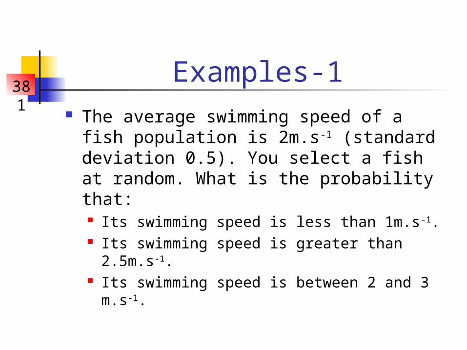
Examples-1 The average swimming speed of a fish

population is 2m.s-1 (standard deviation 0.5). You select a fish at random. What is the probability that: Its swimming speed is less than 1m.s-1. Its swimming speed is greater than 2.5m.s-1. Its swimming speed is between 2 and 3 m.s-

1.

381


population is 2m.s-1 (standard deviation 0.5). You select a fish at random. What is the probability that: Its swimming speed is less than 1m.s-1. Its swimming speed is greater than 2.5m.s-1. Its swimming speed is between 2 and 3 m.s-1.

= P(z < (1-2)/.5) = P(z < -2) = 0.0228

381


population is 2m.s-1 (standard deviation 0.5). You select a fish at random. What is the probability that: Its swimming speed is less than 1m.s-1. Is swimming speed is greater than 2.5m.s-1. Its swimming speed is between 2 and 3 m.s-1.

= P(z > (2.5-2)/.5) = P(z > 1) = 1 - P(z ≤ 1) = 0.159

381



= P( (2-2)/.5 ≤ z ≤ (3-2)/0.5 )= P(0 ≤ z ≤ 2) = P(z ≤ 2) – P(z ≤ 0) = 0.477

381



Why is the normal distribution not entirely satisfactory for this case?

381

Examples-2 In a large group of men 4% are

under 160cm tall and 52% are between 160 cm and 175 cm. Assuming that the heights of men are normally distributed, what are the mean and standard deviation of the distribution?

381

In a large group of men 4% are under 160cm tall and 52% are between 160 cm and 175 cm. Assuming that the heights of men are normally distributed, what are the mean and standard deviation of the distribution?

P(z < (160-μ)/σ ) = 0.04 = P( z < -1.75)P( (160-μ)/σ ≤ z ≤ (175-μ)/σ ) = 0.52 0.56 = P(z ≤ (175-μ)/σ ) = P(z ≤ 0.15 )So: -1.75 = (160-μ)/ σ

0.15 = (175- μ)/ σ μ= 174 , σ= 8

Examples-2

We get these from a

standard normal table

381

Examples-3 An anchovy net can hold 10 t of anchovy.

The mean mass of anchovy school is 8 t with a standard deviation of 2 t. What proportion of schools cannot be fully caught?

Hint: we are interested in the proportion of schools greater than 10t.

ie. 1- P(X ≤ 10) = 1- P(z ≤ (10-8)/2) OR: = 1 - NORMDIST(10,8,2,TRUE)

= 0.159

381 Continuous Probability Distributions (The Normal Distribution-I) QSCI 381 – Lecture 16 (Larson and Farber, Sect 5.1-5.3)

Documents