ENG 351-(EQC 2006/517) rojec Earthquake resistant design of tied-back retaining structures Earthquake resistant design in tied- Kevin McManus, Pacific Geotech Ltd back retaining structures Kevin McManus, Pacific Geotech 1 1

Welcome message from author
This document is posted to help you gain knowledge. Please leave a comment to let me know what you think about it! Share it to your friends and learn new things together.
Transcript
ENG 351-(EQC 2006/517) rojecEarthquake resistant design of tied-back retaining structures Earthquake resistant design in tied-Kevin McManus, Pacific Geotech Ltd
back retaining structuresKevin McManus, Pacific Geotech
1 1
/'.=.- Pacific0=-- Geotech
EARTHQUAKE RESISTANT DESIGN OF
TIED-BACK RETAINING STRUCTURES
EQC RESEARCH REPORT 06/517
Report to EQC Research Foundation
August 2008
Pacific Geotech Ltd
Box 6080
Upper RiccartonChristchurch
Principal Investigator: Kevin McManusPhD FIPENZ(Geotechnical & Structural) CPEng
ABSTRACT
This report considers design procedures for tied-back retaining walls underearthquake loading. Tied-back retaining walls are becoming widely used in NZ to
support permanent excavations on sloping sites iii order to provide level building
platforms for residential and commercial developments. They are also widely used to
support excavations for roadways and other key infrastructure.
Very little guidance is available for the design of tied-back retaining walls to resist
earthquake shaking. Little observational data on the behaviour of tied-back walls
during earthquakes has been published, but, what there is suggests that they behavewell.
A survey ofNew Zealand practice has showed that there is no consistency of
approach and that most designers are relying on a range of different "black box"
computer software with earthquake loading input simply as an additional horizontalforce applied directly to the wall. The appropriateness of this approach isquestionable because the full range of different failure modes is not necessarilyaddressed by the software nor is it always obvious what the software does.
In this study, a seismic design procedure for tied-back retaining walls was synthesizedbased on an existing, widely used, semi-empirical design procedure for gravity designof tied-back walls. The design procedure does not depend on specialist computersoftware.
The design procedure was tested by designing a range of case study walls and thensubjecting them to simulated earthquakes by numerical time-history analysis using
PLAXIS finite element software for soil and rock. The response of the walls to a
variety of real earthquake records was measured including deformations. wall bendingmoments, and anchor forces.
From the results of these analyses, it was observed that all of the wall designs wererobust and performed very well, including those designed only to resist gravity loads.In some cases large permanent deforinations were observed (up to 400 min) but these
were for very large earthquakes (scaled peak ground acceleration of 0.6 g). Iii allcases the walls remained stable with anchor forces safely below ultimate tensile
strength. Wall bending moments reached yield in some cases for the extremeearthquakes, but this is considered acceptable provided the wall elements are detailedfor ductility.
Walls designed to resist low levels of horizontal acceleration (0.1 g and 0.2 g) showed
significant improvements in performance over gravity only designs in terms ofpermanent displacement for relatively modest increases in cost. Walls designed toresist higher levels of horizontal acceleration (0.3 g and ().4 g) showed additionalimprovements in performance but at much greater increases in cost.
Even when walls were designed to resist 100 percent of the peak ground accelerationof a particular earthquake record, significant permanent deformations were stillobserved.
A tentative, detailed design procedure is provided based on the results of the study.
11
ACKNOWLEDGEMENT
This project was funded by the EQC Research Foundation under research grant EQC
06/517. The support and patience of the Foundation is gratefully acknowledged.
Support of the University of Canterbury, Department of Civil Engineering is alsogratefully acknowledged, especially for access to library facilities and for the SeniorFellowship of the Principal Investigator.
DISCLAIMER
This report describes a research project carried out into the behaviour of tied-backretaining walls under seismic loading. The conclusions and recommendationscontained within this report are based on a limited investigation as described in detailin the report. Pacific Geotech Limited and the Principal Investigator do not make anyrepresentations, express or implied, as to the accuracy, completeness, or
appropriateness for use in any particular circumstances, of any of the information
provided, requirements identified, or recommendations made in this report. Pacific
Geotech Limited and the Principal Investigator do not accept any responsibility for
the use or application of, or reliance on any procedures or other information, for anypurpose or reason whatsoever.
111
CONTENTS
ABSTRACT .1
ACKNOWLEDGEMENT n
DISCLAIMER ii
CONTENTS n
1 Introduction... .1
1.1 Overview L
2 Design Procedures .. 1
2.1 Overview 1
2.2 Gravity Design . 3
2.2.1 Possible modes of failure .2
2.2.2 Design procedure for sand . C
2.3 Seismic Design 9
2.3.1 Overview. .9
2.3.2 Mononobe-Okabe Equations 10
2.3.3 Wood Procedure , 10
2.3.4 Comparison between M-O and Wood factors . 12
2.3.5 Practice in New Zealand , 12
2.3.6 Synthesized Design procedure 13
3 Numerical Modelling of Case Studies 15
3.1 Introduction 15
3.2 Methodology... 15
3.3 Time Histories. 16
3.3.1 Overview. 16
3.3.2 Scaling factor€ 18
3.4 Case Study 1: Single Row of Anchors in Sand 21
3.4.1 Case study description 21
-1 -- --
1V
3.4.2 Case 1 a: Gravity design 22
3.4.3 Performance of Case la under gravity and pseudo-static loading.......23
3.4.4 Evaluation of Case la under gravity loading 26
3.4.5 Performance of gravity design Case la under seismic loading ...........26
3.4.6 Case lb: M-O based design to 0.1 g 30
3.4.7 Performance of Case lb under gravity and pseudo-static loading....... 31
3.4.8 Performance of Case 1 b under seismic loading 33
3.4.9 Case 1 c: M-O based design to 0.2 g 36
3.4.10 Performance of Case 1 c under gravity and pseudo-static loading....... 37
3.ill Performance of Case 1 c under seismic loading 38
3.4.12 Case Id: M-0 based design to 0.3 g 41
3.4.13 Performance of Case id under gravity and pseudo-static loading.......42
3.4.14 Performance of Case I d under seismic loading 44
3.4.15 Case le: M-O based design to 0.4 g 47
3.4.16 Performance of Case 1 e under gravity and pseudo-static loading.......48
3.4.17 Performance of Case le under seismic loading 49
3.4.18 Comparison of design cases 52
3.4.19 Conclusions 55
3.5 Case Study 2: Two Rows of Anchors in Sand 56
3.5.1 Case Study Description........................................................................56
3.5.2 Case 2a: Gravity design 57
3.5.3 Performance of Case 2a under gravity and pseudo-static loading.......58
3.5.4 Evaluation of Case 2a under gravity loading 61
3.5.5 Performance of Case 2a under seismic loading 61
3.5.6 Case 2b: M-O based design to 0.1 g 64
3.5.7 Performance of Case 2b under gravity and pseudo-static loading....... 65
3.5.8 Performance of Case 2b under seismic loading 67
V
3.5.9 Case 2c: M-O based design to 0.2 g 69
3.5.10 Performance of Case 2c under gravity and pseudo-static loading....... 71
3.5.11 Performance of Case 2c under seismic loading 72
3.5.12 Comparison ofdesign eageR 74
3.5.13 Conclusions 78
3.6 Case Study 3: Two Rows of Anchors in Sand with Extended Anchors......79
3.6.1 Case Study Description 79
3.6.2 Case 3a: Gravity design ...... 79
3.6.3 Performance of Case 3a under gravity and pseudo-static loading.......81
3.6.4 Evaluation of Case 3a under gravity loading.. 82
3.6.5 Performance of Case 3a under seismic loading 82
3.6.6 Case 3b: M-O based design to 0.1 g 85
3.6.7 Performance of Case 3b under gravity and pseudo-static loading....... 86
3.6.8 Performance of Case 3b under seismic loading 87
3.6.9 Case 30: M-O based design to 0.2 g 90
3.6.1() Performance of Case 3c under gravity and pseudo-static loading....... 91
3.6.11 Performance of Case 3c under seismic loading 92
3.6.12 Comparison ofdesign eageR 95
3.6.13 Conclusions 97
4 Design Guidelines... 98
4.1 Overview 98
4.2 Seismic Design Accelerations 99
4.3 Proposed Design Guidelines for "Sand" soils 100
5 Summary and Conclusions 104
6 Recommendations for Future Research 108
References 109
Appendix A 111
V1

A.1 Design calculations for case study Sand la
A.2 Design calculations for case study Sand 1 b
A.3 Design calculations for case study Sand 1 c
A.4 Design calculations for case study Sand 1 d
A.5 Design calculations for case study Sand 1 e
Appendix B..
B. 1 Design calculations for case study Sand 2a
B.2 Design calculations for case study Sand 2b
B.3 Design calculations for case study Sand 2c
Appendix C
C.1 Design calculations for case study Sand 3a
C.2 Design calculations for case study Sand 3b
C3 Design calculations for case study Sand 3c
- Gravity based design .........111
- M-0 based design 0.1 g..... 119
- M-O based design 0.2 g.....126
- M-O based design 0.3 g..... 133
- M-O based design 0.4 g.....140
147
- Gravity based design .........147
- M-O based design 0.1 g..... 154
- M-O based design 0.2 g.....161
168
- Gravity based design .........168
- M-O based design 0.1 g..... 170
- M-O based design 0.2 g.....172
Vll
EQC 06/477 Tied Back Retaining Walls August 2008
1 Introduction
Kramer [1996] has summarised the limited research available on this topic. Very fewreports of the behaviour of tied back walls during earthquakes are available. Ho et. al.[1990] surveyed ten anchored walls in the Los Angeles area following the Whittierearthquake of 1987 and concluded that they performed very well with little or no lossof integrity.
Numerical analyses of tied-back walls have been performed by Siller and Frawley[19921 and Siller and Dolly [1992] who found that walls with stiff, more closelyspaced anchors develop smaller and more uniform permanent displacements thanwalls with softer anchors and greater vertical spacing of anchors. Walls designed forhigher static earth pressures were also found to develop smaller permanentdisplacement than walls designed to lower static pressures. Walls with higher initialanchor preloads were found to develop smaller permanent displacements than wallswith lower preloads.
Fragaszy et. al. [1987] found that wall elements that extend into the foundation soilsmay be subjected to very high bending moments at the base because of phasedifferences in movements between the top and bottom ofthe wall. Inclined anchorsextending below the base o f the excavation may become highly stressed when thebonded end of the anchor embedded in soil moves out of phase with the wall face.
Detailed design guidance has been provided by Sabatini et. al. [19991 within a generaldesign manual for tied-back walls prepared for the US Department of Transportation,Federal Highway Administration. This manual is in wide use within the US and isgaining increasing acceptance within New Zealand. They recommend the use of thepseudo-static so called Mononobe-Okabe method [Okabe, 1926; Mononobe andMatsuo, 1929] to calculate earthquake induced active earth pressures acting againstthe back face of a tied-back wall. A seismic coefficient from between one-halfto
two-thirds of the peak horizontal ground acceleration (().5 PGA to ().67 PGA) isrecommended to provide a wall design that wililimit deformations to small valuesacceptable for highway facilities.
Sabatini et. al. [1999] recommends that brittle elements of the wall system (thegrout/tendon bond) should be governed by the peak ground acceleration "adjusted toaccount for the effect of local soil conditions and the geometry of the wall" and afactor of safety of 1.1 applied. Design of ductile elements, including the tendon,should be governed by the cumulative permanent seismic deformation. Theyrecommend that, based on studies using Newmark type sliding wedge analyses,
ductile elements should be designed using forces calculated by pseudo-static analysisusing a seismic coefficient of 0.5 PGA with a factor o f safety of 1.1 applied. Thelength of the ground anchors may need to be increased beyond that calculated forstatic design with the anchor bond zone located outside of the Mononobe-Okabeactive wedge ofsoil.
The use of the Mononobe-Okabe method to calculate earth pressure for design of tied-back walls has the advantage of being straightforward and is widely used for design ofgravity retaining walls. However, it is based on limiting equilibrium and the
1

EQC 06/477 Tied Back Retaining Walls August 2008
development of an active failure wedge of soil that is at odds with the designprocedure for static loads for tied-back walls. The recommendation to place the bondzone of the anchors behind the active soil wedge means that the wall is not free tomove with the wedge, as assumed by the Mononobe-Okabe procedure.
1.1 Overview
This project has studied the performance oftied-back retaining walls by use ofnumerical time-history analysis using PLAXIS finite element software for soil androck [Brinkgreve & Vermeer, 1988]. Too few field studies from actual earthquakesare available to make meaningful conclusions and testing of scaled down models on ashaking table is of limited ilse because of the impossibility of satisfying scaling lawswithout increasing the gravity field in a centrifuge. Numerical analysis ofproblems ingeomechanics has become a recognised tool for exploring soil-structure interactionproblems and is probably the only practical way to investigate the complexity of tied-back wall behaviour during earthquake shaking.
The project has focussed on developing a rational and practical design procedure thenverifying the procedure by considering different case studies of tied-back walls. Thecase study walls were designed using the proposed procedure and then subjected to
different earthquake time-histories using PLAXIS. The performance ofeach walldesign was assessed for each earthquake by monitoring various key parametersincluding displacement, wall bending moments, and anchor forces.
After assessing the performance of the various wall designs, the proposed designprocedure was critically assessed and final guidelines and recommendations made.
F,very wall design case in practice is different in some way from every previousdesign. It was impossible within the constraints of time and budget to consider everypossible wall circumstance. Instead, the case studies were based on the simple, caseof a deep uniform sand soil deposit with suitably generic properties. Thissimplification is both necessary and desirable because it allows the basic trends inwall performance to be observed without "clutter" from a myriad of differentparameters.
At the commencement of the project a survey was undertaken to identify availablepublished design procedures and to identify current New Zealand practice. Thisinformation was used to identify the most rational design procedure and to clarify andrefine such a procedure as necessary. The case study designs and analyses then wereundertaken to prove or otherwise the efficacy and safety of the design procedure.
2
EQC 06/477 Tied Back Retaining Walls August 2008
2 Design Procedures
2.1 Overview
Tied-back retaining walls were used originally as a substitute for braced retainingwalls in deep excavations. Ground anchor tie-backs were used to replace bracing
struts that caused congestion and construction difficulty within the excavation.Design procedures evolved from those developed for braced excavations and aretypically based on the so-called "apparent earth pressure" diagrams of Terzaghi andPeck [1967] and Peck [1969]. These diagrams were developed empirically from
measurements of loads imposed on bracing struts during deep excavations in sands in
Berlin, Munich, and New York; in soft to medium insensitive glacial clays in
Chicago; and in soft to medium insensitive marine clays iii Oslo.
These original "apparent earth pressure diagrams" were not intended by the authors to
be a realistic representation of actual earth pressures against a wall but to be"...merely an artifice for calculating values of the strut loads that will not be exceeded
in any real strut in a similar open cut. In general, the bending moments in the sheetingor soldier piles, and in wales and lagging, will be substantially smaller than those
calculated from the apparent earth pressure diagram suggested for determining strut
loads."[Terzaghi & Peck, 1967].
Since 1969, remarkably few significant modifications to this original work have beenadopted in practice. More recently, Sabatini et. al. [1999] proposed a more detaileddesign procedure based on the apparent earth pressure approach intended specifically
for pre-tensioned, tied-back retaining walls in a comprehensive manual prepared for
the US Department of Transportation, Federal Highway Administration. This manualis in wide use within the US and is gaining increasing acceptance within NewZealand.
A detailed and well proven design procedure for walls under gravity loading is given
in this manual which will be referred to throughout this report as the "FHWAprocedure". The manual also makes suggestions for design of tied-back walls to resistearthquake loading although a detailed procedure is not given.
Increasingly, practitioners are relying on computer "black box" software to design
tied-back walls with methodologies that range from fully elastic "beam-on-elastic-foundation" approaches to limiting equilibrium approaches. Caution is required when
66
using black box" software to ensure that all possible failure modes have beenconsidered.
2.2 Gravity Design
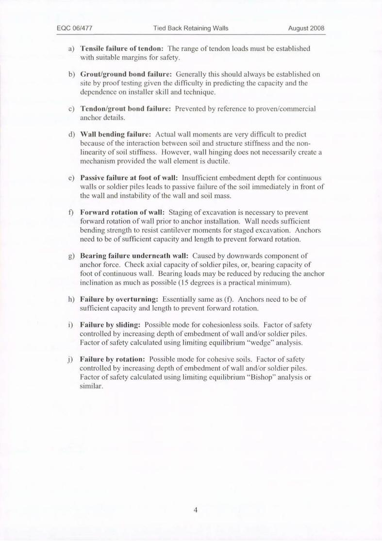
2.2.1 Possible modes of failure
Possible modes of failure for tied-back retaining walls are illustrated in cartoon
fashion iii Figure 2.2.1 (a). A complete design procedure needs to address each ofthese modes offailure
3
EQC 06/477 Tied Back Retaining Walls August 2008
a) Tensile failure of tendon: The range of tendon loads must be establishedwith suitable margins for safety.
b) Grout/ground bond failure: Generally this should always be established onsite by proof testing given the difficulty in predicting the capacity and the
dependence on installer skill and technique.
C) Tendon/grout bond failure: Prevented by reference to proven/commercialanchor details.
d) Wall bending failure: Actual wall moments are very difficult to predictbecause of the interaction between soil and structure stiffness and the non-
linearity of soil stiffness. However, wall hinging does not necessarily create a
mechanism provided the wall element is ductile.
e) Passive failure at foot of wall: Insufficient embedment depth for continuouswalls or soldier piles leads to passive failure of the soil immediately in front of
the wall and instability of the wall and soil mass.
f) Forward rotation of wall: Staging of excavation is necessary to prevent
forward rotation of wall prior to anchor installation. Wall needs sufficientbending strength to resist cantilever moments for staged excavation. Anchorsneed to be of sufficient capacity and length to prevent forward rotation.
g) Bearing failure underneath wall: Caused by downwards component ofanchor force. Check axial capacity of soldier piles, or, bearing capacity offoot of continuous wall. Bearing loads may be reduced by reducing the anchor
inclination as much as possible (15 degrees is a practical minimum).
h) Failure by overturning: Essentially same as (f). Anchors need to be of
sufficient capacity and length to prevent forward rotation.
i) Failure by sliding: Possible mode for coliesionless soils. Factor of safetycontrolled by increasing depth of embedment of wall and/or soldier piles.
Factor of safety calculated using limiting equilibrium "wedge" analysis.
j) Failure by rotation: Possible mode for cohesive soils. Factor ofsafetycontrolled by increasing depth ofembedment ofwall and/or soldier piles.Factor of safety calculated using limiting equilibrium "Bishop" analysis orsiiilar.
4
EQC 06/477 Tied Back Retaining Walls August 2008
6(a) Tensile failure oftendon
{b) Puflout failure ofgroutlground bond
(c) Pullout failure of
tendon/grout bond
L(d) Failure of wan in bending
(e) Failure of wall due toinsufficient passive capacity
(f) Faiture by forward rotation(cantilever before first anchor installed)
(g} Failure due to insufficientaxial capacity
(h) Failure by overturning
(i) Failure by sliding 0) Rotational failure ofground mass
via:,dzefZv /
-Aclive are /
loading wall //
Envelcpe d deepes: points ofpoternal falure mechanismswhich require 5098 anchor
force lor *Uability
Adivo /KN,u k>Jading 8,111
16<Z ,4_ Uimmurn estance from wai &0- st:Irt of anchot bond langth
5

EQC 06/477 Tied Back Retaining Walls August 2008
Figure 2.2.1 (a) Possible modes of failure for tied-back retaining walls [Sabatini et.al., 1999].
2.2.2 Design procedure for sand
The following procedure addresses each ofthe above failure modes systematically
(for the gravity load case) and is based on the FHWA procedure with minormodifications and clarifications where noted. It is assumed herein that the wall and
retained soil are fully drained. This procedure is intended to be readily calculated byhand, although use of calculation software such as Mathcad or Excel will be useful for
design iterations. Example calculations using Mathcad for the case studies are includein the appendices.
a) Initial trial geometry: The depth of excavation and depth to each row of
anchors needs to be estimated as a first step, based on experience or trial anderror. Typically, for stronger soils, the first row will be at a depth of 2 m with
subsequent rows at 5 m intervals.
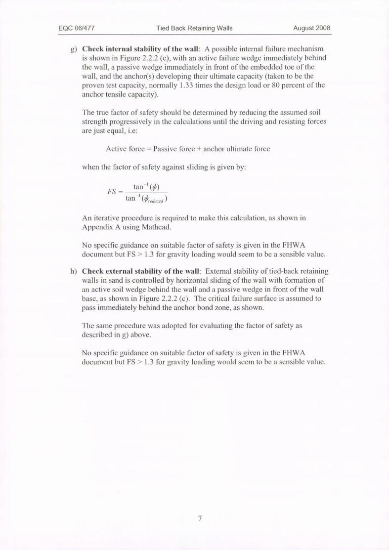
b) Prepare apparent earth pressure diagram: As shown in Figure 2.2.2 (a).
Note that K is calculated as follows: K =tan 2 45 - -0-The Rankine value of KA is for frictionless walls but is used here by tradition
because ofthe empirical nature ofthe apparent earth pressure formulation.
Also, the wall will generally move downwards with any developing active soilwedge.
c) Calculate anchor design load: As shown in Figure 2.2.2 (a).
d) Calculate wall base reaction, R: As shown in Figure 2.2.2 (a).
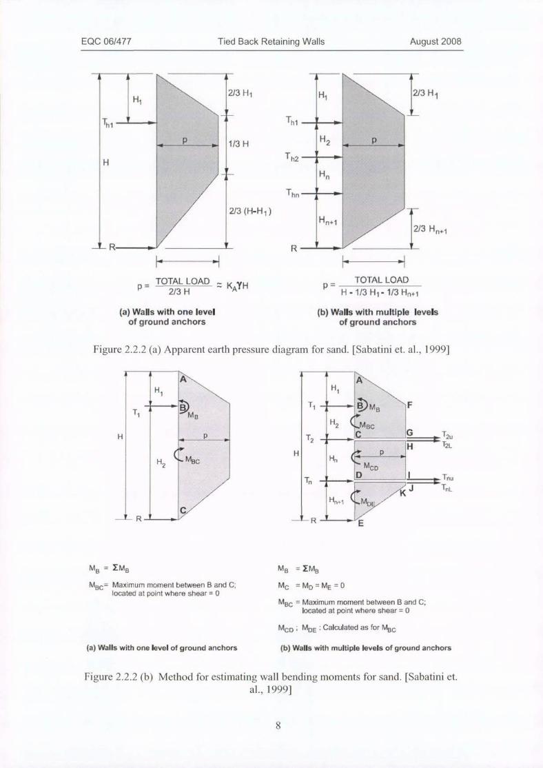
e) Calculate wall section bending moment: From the apparent earth pressure
diagram as shown in Figure 2.2.2 (b). These methods are considered to
provide conservative estimates of the calculated bending moments, but maynot accurately predict the exact locations of the maxima. FHWA document
recommends an allowable stress of Fb = 0.55 Fy for steel soldier piles. ForNew Zealand design procedures using load and resistance factor design
(LRFD) principles and for a strength reduction factor for steel sections of 0.8,
an equivalent load factor ofa = 0.8/0.55 = 1.45 is implied. However, forconsistency with NZS 4203 (see discussion elsewhere) a load factor of 1.6 was
adopted for this study for the purpose of sizing wall structural elements.
f) Determine depth of embedment: Calculate required depth of embedn-tent for
soldier Files to resist wall base reaction (R) using Broms [1965] or similar, or,for continuous walls using passive resistance from Coulomb theory or log-
spiral theory such as NAVFAC DM-7. FHWA document recommends a
factor of safety of 1.5 for these calculations. For this study, a strength
reduction factor of 3 is applied to the Broms [1965] formulation because of the
large plastic strains required to mobilise the fu 11 passive resistance. Use of this
reduction factor was found to give realistic embedment depths consistent with
avoidance of wedge failures and better control of displacements.
6
EQC 06/477 Tied Back Retaining Walls August 2008
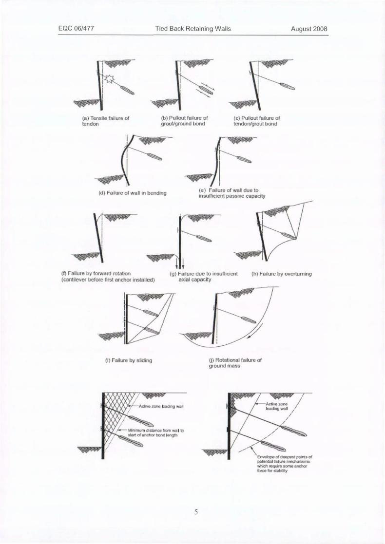
g) Check internal stability of the wall: A possible internal failure mechanism
is shown in Figure 2.2.2 (c), with an active failure wedge immediately behindthe wall, a passive wedge immediately in front of the embedded toe of thewall, and the anchor(s) developing their ultimate capacity (taken to be theproven test capacity, normally 1.33 times the design load or 80 percent of theanchor tensile capacity).
The true factor of safety should be determined by reducing the assumed soilstrength progressively in the calculations until the driving and resisting forces
are just equal, i.e:
Active force = Passive force + anchor ultimate force
when the factor of safety against sliding is given by:
FS =tan-1 (0)
tan 1 (ere,hic·ed )
An iterative procedure is required to make this calculation, as shown inAppendix A using Mathcad.
No specific guidance on suitable factor of safety is given in the FHWAdocument but FS > 1.3 for gravity loading would seem to be a sensible value.
lit) Check external stability of the wall: External stability of tied-back retaining
walls in sand is controlled by horizontal sliding of the wall with formation ofan active soil wedge behind the wall and a passive wedge in front of the wall
base, as shown in Figure 2.2.2 (c). The critical failure surface is assumed to
pass immediately behind the anchor bond zone, as sliown.
The same procedure was adopted for evaluating the factor of safety as
described in g) above.
No specific guidance on suitable factor of safety is given in the FHWAdocument but FS > 1.3 for gravity loading would seem to be a sensible value.
7
EQC 06/477 Tied Back Retaining Walls August 2008
hA : 8 8
2/3 H 1 H1 16 \\ 2/3 H 1Hl 9 46 9\\Thl ' p
1 1/3 n -4-.
H
P
2/3 (H-H 1)Hn+1
2/3 Hn+1
R ' 5/t 11 4
= TOTAL LOAD2/3 H
i KAYH P=TOTAL LOAD
H - 1/3 Hi - 1/3 H.,+1
(a) Walls with one levelof ground anchors
(b) Walls with multiple levelsof ground anchors
Figure 2.2.2 (a) Apparent earth pressure diagram for sand. [Sabatini et. al., 1999]
. A
Tl .
H
IR w
MB = IMB
A
H H1
1
T 7 • MBH2 GBC
P T C G R T=uH T2L
H2 MBC H P
1 McDTni
Hn+1
2-R ' =E
/K
MB = IMBMBC= Maximum moment between Band C, MC =MD=ME=0
located at point where shear = 0MBC = Maximum moment between B and C;
located at point where shear = 0
McD ; MDE ; Calculated as for MBC
(a) Walls with one level of ground anchors (b) Walls with multiple levels of ground anchors
Figure 2.2.2 (b) Method for estimating wall bending moments for sand. [Sabatini et.
aL, 19991
Thl8
P
Th2
Thn
8

EQC 06/477 Tied Back Retaining Walls August 2008
j
Wall---4--Internal /
/' Stability /
H / External
p:/ Stability
j
d
Fig 2.2.2 (c) Internal and external mechanisms for tied back walls.
2.3 Seismic Design
2.3.1 Overview
Little guidance is available for the design of tied-back retaining walls to resist seismicactions. Gravity retaining walls are normally designed using a pseudo-staticapproach: The active wedge ofsoil immediately behind the wall has an additionalpseudo-static force component equal to the mass of soil within the wedge multipliedby acceleration. Typically, the resulting forces are resolved to derive a new criticalwedge geometry and necessary wall pressure to achieve equilibrium, as in theMononobe-Okabe (M-O) theory [Okabe, 1926; Mononobe and Matsuo, 1929].
For retaining walls that are rigid and unable to move sufficiently to allow soil yieldingand development of a Rankine condition behind the wall (e.g. buried basements), atheoretical linear elastic solution for soil pressure derived by Wood [19731 is normallyused to calculate dynamic soil pressure.
These two approaches represent, perhaps, an upper and lower bound of what theresulting dynamic soil load might be against a tied-back retaining wall.
The only published advice specific to design of tied-back retaining walls was foundwithin the FHWA manual [Sabatini et. al., 1999]. FHWA recommend use of thepseudo-static Mononobe-Okabe (M-O) theory to design tied-back retaining walls butdo not give a detailed procedure. Nor is such a procedure obvious because therecommended design procedure for tied-back walls under gravity loading is based onempirical "apparent earth pressure" diagrams.
9
EQC 06/477 Tied Back Retaining Walls August 2008
The FHWA manual states that the design of brittle elements (e.g. the grout/tendonbond) should be governed by the peak force (i.e. corresponding to peak groundacceleration, PGA). Design of ductile elements (e.g. tendons, steel sheet piles, soldierpiles) should be governed by cumulative permanent seismic deformation, or in lieu ofsucli analysis, design should be based on 0.5 times the PGA. However, no advice isgiven as to how the "peak force" might be calculated.
Given that the anchor tendons are, effectively, long springs with little mass then thereseems no reason why they should be subject to high peak forces and should respondonly to elongation from gross movements within the soil mass.
Neither of the formulations (Wood or M-O) for calculating wallloads during shakingtake any account of the flexibility of the wall and the likely kinematic effects and soil-structure interactions.
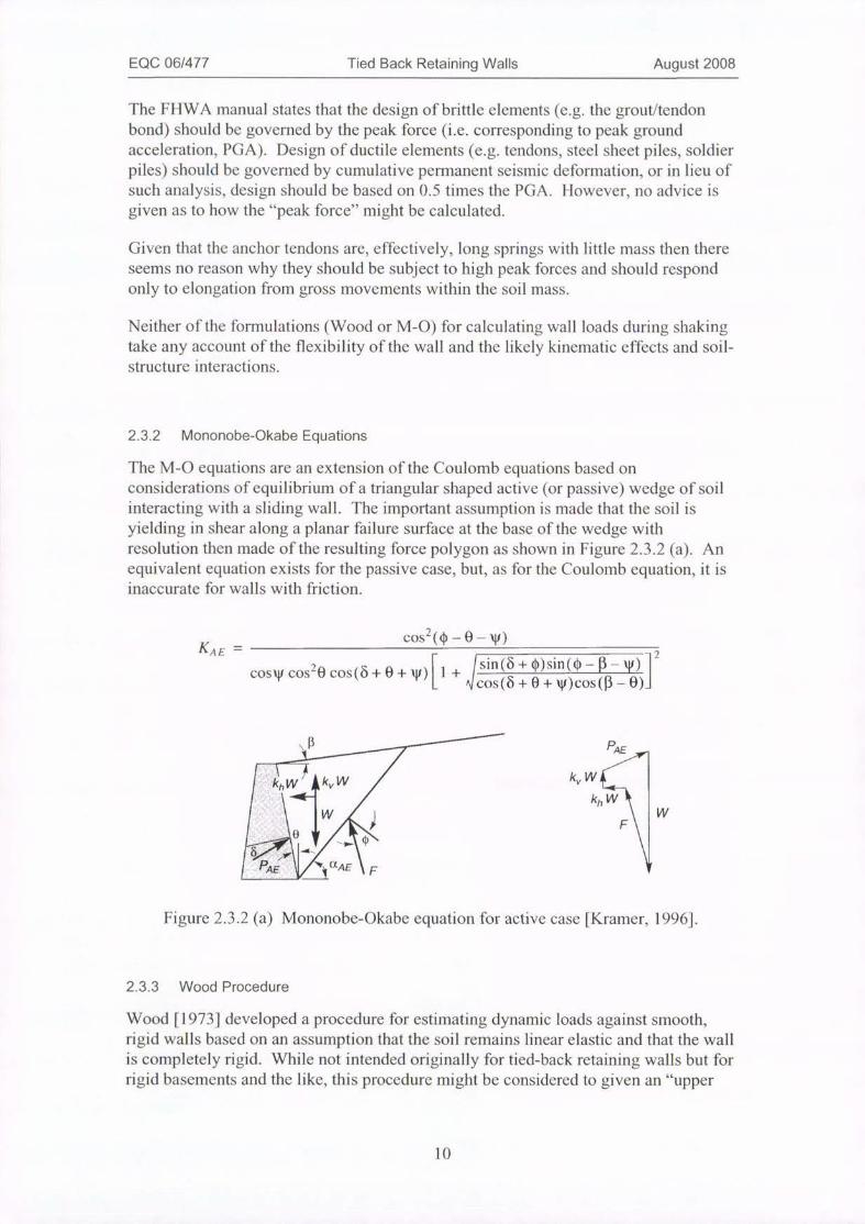
2.3.2 Mononobe-Okabe Equations
The M-O equations are an extension of the Coulomb equations based onconsiderations of equilibrium of a triangular shaped active (or passive) wedge of soilinteracting with a sliding wall. The important assumption is made that the soil isyielding in shear along a planar failure surface at the base of the wedge withresolution then made of the resulting force polygon as shown in Figure 2.3.2 (a). Anequivalent equation exists for the passive case, but, as for the Coulomb equation, it isinaccurate for walls with friction.
COS2(¢-0-WKAE =
cos 4,cosiecos(8-1-0.+ 4/) 1 4- isin(64-*)sin(¢)-- B--4/) 1Ncos(6 +0+ W)COS(13 - 0)]
2
PAE
W4kvw /1 ..t.,dr -1 0 ' / f 6
FAE 1/3 (XAE \ F
kvW <kj
\ W
FLFigure 2.3.2 (a) Mononobe-Okabe equation for active case IKramer, 19961
2.3.3 Wood Procedure
Wood [1973] developed a procedure for estimating dynamic loads against smooth,rigid walls based on an assumption that the soil remains linear elastic and that the wallis completely rigid. While not intended originally for tied-back retaining walls but forrigid basements and the like, this procedure might be considered to given an "upper
10
EQC 06/477 Tied Back Retaining Walls August 2008
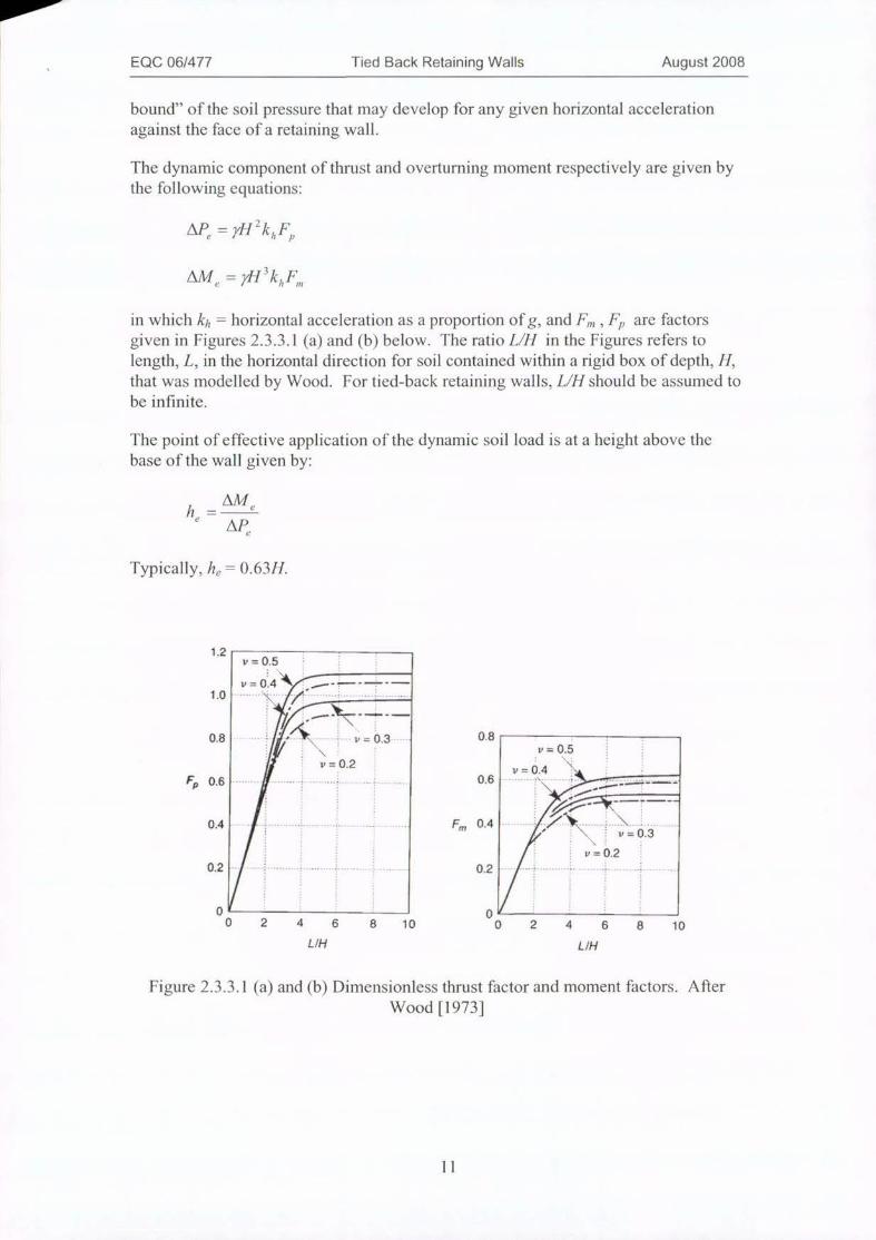
bound" of the soil pressure that may develop for any given horizontal accelerationagainst the face of a retaining wall.
The dynamic component of thrust and overturning moment respectively are given bythe following equations:
Ape = #11 k j, FP
AM e = 9 fAkj Fm
in which kh = horizontal acceleration as a proportion ofg, and Pm, Fp are factorsr.
given in Figures 2.3.3.1 (a) and (b) below. The ratio L/H in the Figures refers to
length, L, in the horizontal direction for soil contained within a rigid box of depth, H,that was modelled by Wood. For tied-back retaining walls, L/H should be assumed tobe infinite.
The point of effective application of the dynamic soil load is at a height above thebase of the wall given by:
h=AM
APe
Typically, he = 0.63H.
12v =05
0.8 p = 0.3 08
v= 0.2V=
0.6
Fm 0.4
0 00 2 4 6 8 10 0
L/H
v = 0.5
V=
2 4
L/H
v = 0.3
0.2
8 10
Figure 2.3.3.1 (a) and (b) Dimensionless thrust factor and moment factors. After
Wood [1973]
11

EQC 06/477 Tied Back Retaining Walls August 2008
2.3.4 Comparison between M-O and Wood factors
The additional nominal wallloading caused by a pseudo-static horizontal accelerationwas calculated using either the M-0 or the Wood equations as shown in Table 2.3.4(a) for the case of walls in sand with 0 = 35 degrees.
Table 2.3.4 (a) Comparison of nominal wallloading caused by pseudo-staticacceleration
Horizontal Acceleration Wood Mononobe-Okabe
kh kah - kav= 0.3 0= 35
0.1 0.1 0.06
0.2 0.2 0.13
0.3 0.3 0.21
0.4 0.4 0.31
At lower levels of acceleration, the M-0 equation gives about 'h the load of the Woodequation, increasing to -A at 0.4 g. The M-O equation is expected to give much lowerloading because it assumes that soil shear strength is fully mobilised to resist theacceleration.
2.3.5 Practice in New Zealand
Given the paucity of guidance in the literature, it was decided to conduct a survey tofind out how practitioners were designing tied-back walls to resist earthquakes incurrent practice.
Current practice in New Zealand was surveyed by conducting a series of personalinterviews with senior staff in the largest practices and also from the author'sexperience in numerous design reviews. Little consistency in approach was evident,with most respondents relying on "black box" computer software that does notspecifically consider earthquake loading.
The most commonly used software package is "WALLAP" [Copyright 2002, D.L.Borin, Geosolve, UK]. This software combines limiting equilibrium analysis toBritish and European standards to compute factors of safety coupled with a 1 -D"beam on elastic foundation" or finite element analysis to compute wall elementstresses and deformations.
Earthquake "loads" are typically being input as static loads applied to nodes. Thecalculation of the pesudo-static loads are made using either the M-0 equations or theWood [1973.] analysis according to the judgement of the designer.
Typically, the free length ofthe anchors are located according to the inclination of theCoulomb, gravity only active soil wedge, with no increase to allow for the flatteningof the active wedge under acceleration (at least one major consultancy).
12
EQC 06/477 Tied Back Retaining Walls August 2008
(Note: A new version of "WALLAP" has recently been released which allows inputof earthquake accelerations directly, although the methodology for computiiigearthquake response is not known).
2.3.6 Synthesized Design procedure
With no detailed procedure for the design of tied-back walls to resist earthquakeloading available, it was necessary to synthesize a trial procedure. A procedure wassynthesized based on the FHWA procedure for gravity loading by applying thefollowing rationale.
1. Since the apparent earth pressure used for wall design in gravity loading iscalculated based on Ka, the Rankine coefficient of active earth pressure,simply substitute Kae, the M-0 coefficient of active earth pressure underearthquake acceleration to calculate an equivalent apparent earth pressure forthe earthquake design case.
2. Anchor free lengths are normally extended to beyond the location of theCoulomb active wedge slip plane when designing tied-back walls for gravityloading. Therefore, extend the anchor free length to beyond the equivalent M-O slip plane for earthquake loading.
3. The M-0 equations should also be used when checking the external stabilityof a wall.
The following detailed procedure was adopted on a trial basis for the case studiesexamined in this project. Based on the results of the time history analyses, additionalminor recommendations and improvements were made and these are included in thefinal recommended procedure of Section 4.
a) Initial trial geometry: The depth of excavation and depth to each row ofanchors needs to be estimated as a first step, based on experience or trial anderror. Typically, for stronger soils, the first row will be at a depth of 2 m withsubsequent rows at 5 m intervals.
b) Prepare apparent earth pressure diagram: As shown in Figure 2.2.2 (a).Note that KA is calculated using the M-O equation with the selected designpseudo-static acceleration. The wall is assumed to be frictionless (i.e. the wallis likely to move downwards with any active soil wedge).
c) Calculate anchor design load: As shown in Figure 2.2.2 (a).
d) Calculate wall base reaction, 12: As shown in 2.2.2 (a)
e) Calculate wall section bending moment: From the apparent earth pressurediagram as shown in Figure 2.2.2 (b). A load factor of 1.6 is recommended forthe purpose of sizing wall structural elements using New Zealand standards.
f) Determine depth o f embedment: Calculate required depth of embedment forsoldier piles to resist wall base reaction (R) using Broms [1965] (but
13
EQC 06/477 Tied Back Retaining Walls August 2008
calculating Kp using the M-0 equations), or, for continuous walls usingpassive resistance from M-0 Okabe theory. A strength reduction factor of 3 isrecommended to be applied to these calculations because of the large plasticstrains required to mobilise the full passive resistance. Use ofthis reductionfactor has been found to give realistic embedment depths consistent withavoidance of wedge failures and better control ofdisplacements.
g) Cheek internal stability of the wall: A possible internal failure mechanismis shown in Figure 2.2.2 (c), with an active failure wedge immediately behindthe wall, a passive wedge immediately in front of the embedded toe ofthewall, and the anchor(s) developing their ultimate capacity (taken to be theproven, test capacity, normally 1.33 times the design load or 80 percent of theanchor tensile capacity).
The true factor of safety may be determined by progressively reducing theassumed soil strength in the calculations until the driving and resisting forcesarejustequal, i.e:
Active force = Passive force + anchor ultimate force
when the factor of safety against sliding is given by:
FS=tan'(0)
tan i (0;.edi,c·ed )
For the earthquake load case using pseudo-static design, a minimum factor ofsafety of 1.lis recommended, but not less than the factor of safety againstexternal stability.
h) Set "free" length of anchor tendons: The "free" length of the anchortendons should extend beyond the active soil wedge defined by the M-0theory and originating at the base of the wall or the embedded soldier piles asindicated in Figure 2.2.2 (c).
i) Check external stability of the wall: External stability of tied-back retainingwalls in cohesionless soil is controlled by horizontal sliding ofthe wall withformation of an active soil wedge behind the wall and a passive wedge in frontofthe wall base, as shown in Figure 2.2.2 (c). The critical failure surface isassumed to pass immediately behind the anchor bond zone, as shown.
For the earthquake load case using pseudo-static design, a minimum "true"factor of safety of 1.0 based on mobilised soil shear strength is recommended.
j) Note: When calculating passive soil resistance, the interface friction angle
should be set to be no more than ¢/2. Use of higher values is notrecommended because the resulting values of passive resistance will be11 nrcalistically high.
14
EQC 06/477 Tied Back Retaining Walls August 2008
3 Numerical Modelling of Case Studies
3.1 Introduction
No good case study data is available regarding the performance of tied-back retainingwalls in real earthquakes. No data was found for physical model studies for tied-backretaining walls in simulated earthquakes. Modelling of geotechnical systems isdifficult, in any case, because the laws of physical similitude require that modelexpenments be carried out either at very large scale, or, at small scale under highaccelerations in a centrifuge.
Numerical modelling in geotechnical engineering has become an accepted research
tool and is viewed as a practical substitute to physical modelling for many problems.For study of tied-back retaining walls under earthquake loading, numerical modellingmay be the only practical method for realistic simulation given the complexities of thewall construction.
For this study, two representative tied-back wall designs have been modelled
numerically: A simple wall with one level of tie-back anchors and a more complexwall with two levels of anchors. Simplified soil conditions have been chosen to berepresentative of real conditions. Obviously, in practice, much more complexstratigraphies are likely to be encountered, but the objective herein is to gainunderstanding ofthe fundamentals of wall performance without introducing confusionfrom complex stratigraphy.
Detailed design ofthe walls was made in accordance with the trial design procedurewith slight variations and the performance of each under both static gravity andseismic conditions was determined using PLAXIS finite element software for soil androck mechanics [Brinkgreve & Vermeer, 1988]. Earthquake performance wasdetermined by subjecting each design to time histories of shaking from several realearthquake records scaled to different levels of peak ground acceleration (PGA).
3.2 Methodology
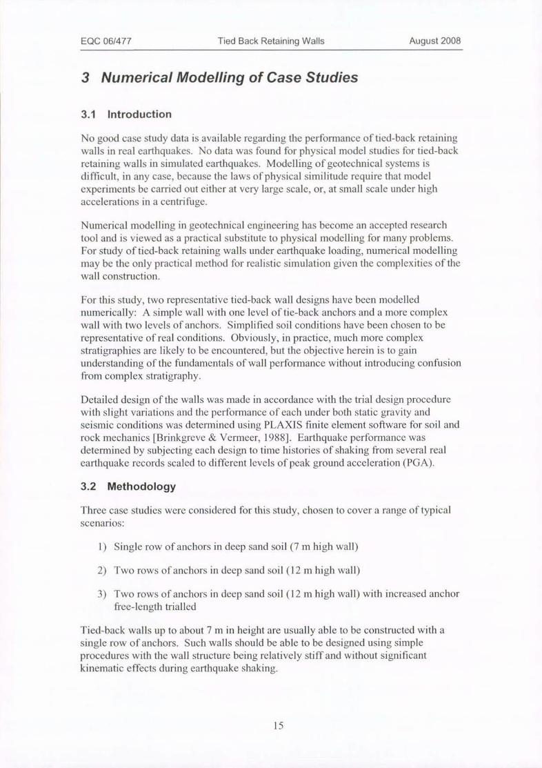
Three case studies were considered for this study, chosen to cover a range of typicalscenarios:
1) Single row of anchors in deep sand soil (7 m high wall)
2) Two rows of anchors in deep sand soil ( 12 m high wall)
3) Two rows of anchors in deep sand soil (12 m high wall) with increased anchorfree-length trialled
Tied-back walls up to about 7 in in height are usually able to be constructed with asingle row of anchors. Such walls should be able to be designed using simpleprocedures with the wall structure being relatively stiff and without significantkinematic effects during earthquake shaking.
15
EQC 06/477 Tied Back Retaining Walls August 2008
As walls become higher, with multiple rows of anchors, the wall elements become
relatively more flexible and kinematic effects during shaking are likely to become
more important. Verification of simple quasi-static design procedures for such wallsis an iinportant objective of this study.
Tied-back walls up to about 12 m in height are typically able to be supported by two
rows of anchors. Walls greater in height than 12 m will usually require three or morerows of anchors and permanent walls of such height are not often encountered inpractice. In this study, a 12 m high wall with two rows ofanchors is studied under
gravity and earthquake loading conditions. Walls greater in height than this shouldperhaps be the subject of special study if they are required to resist high seismic loads.
The uniform sand soil used for this study was intended to be representative of
granular soil profiles in general. Obviously, much more complex stratigraphies willbe encountered in practice, but the reason for simplifying the stratigraphy was to
simplify the model as far as practicable to assist with interpretation of the results.
3.3 Time Histories
3.3.1 Overview
Three earthquake accelerogram records were selected to use as input motions for the
time history analyses of this project:
• Loma Prieta Earthquake of 18 Oct 1989, MI = 6.9, Dist = 43km, PGA = 215crn/s/s
• Parkfield Earthquake of 28 Sept 2004, Mi = 6.0, Dist = 11.6km, PGA =300.0 cm/s/s
• Sierra Madre Earthquake 28 Jun 1991, Mt = 5.8, Dist= 18. lkm, PGA =273.9cm/s/s
The objective in using multiple records was to include the influence ofearthquake
variability on wall performance.
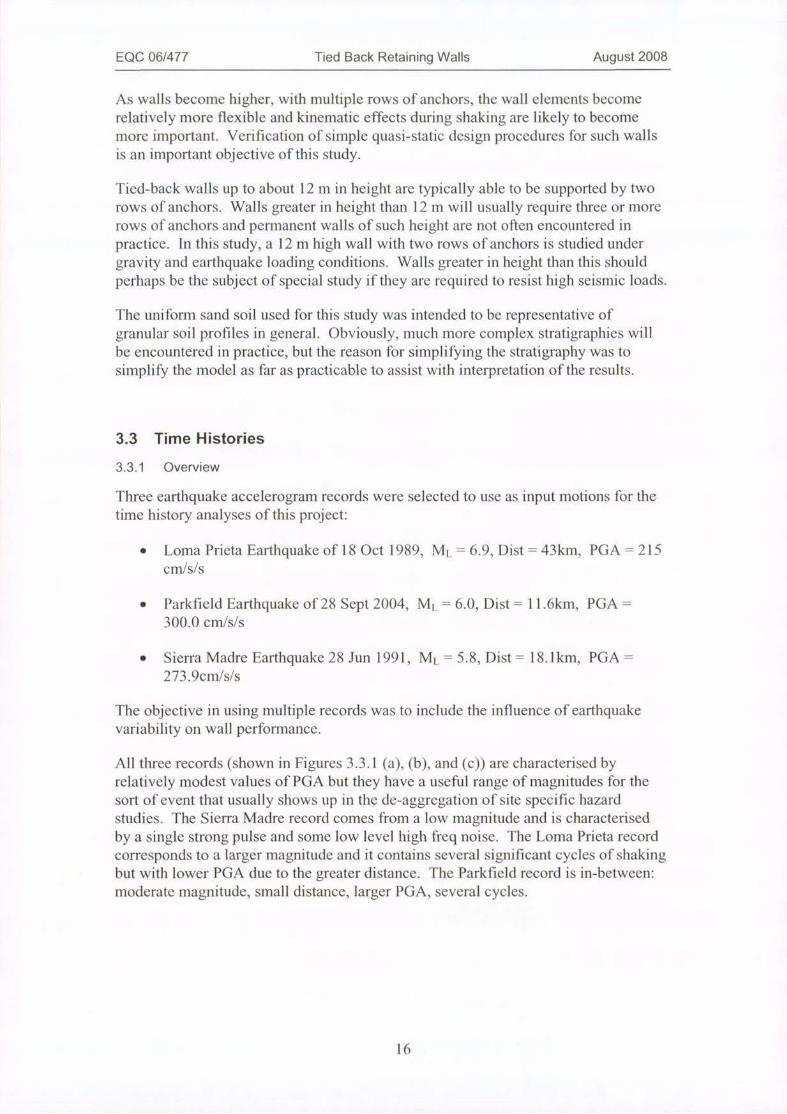
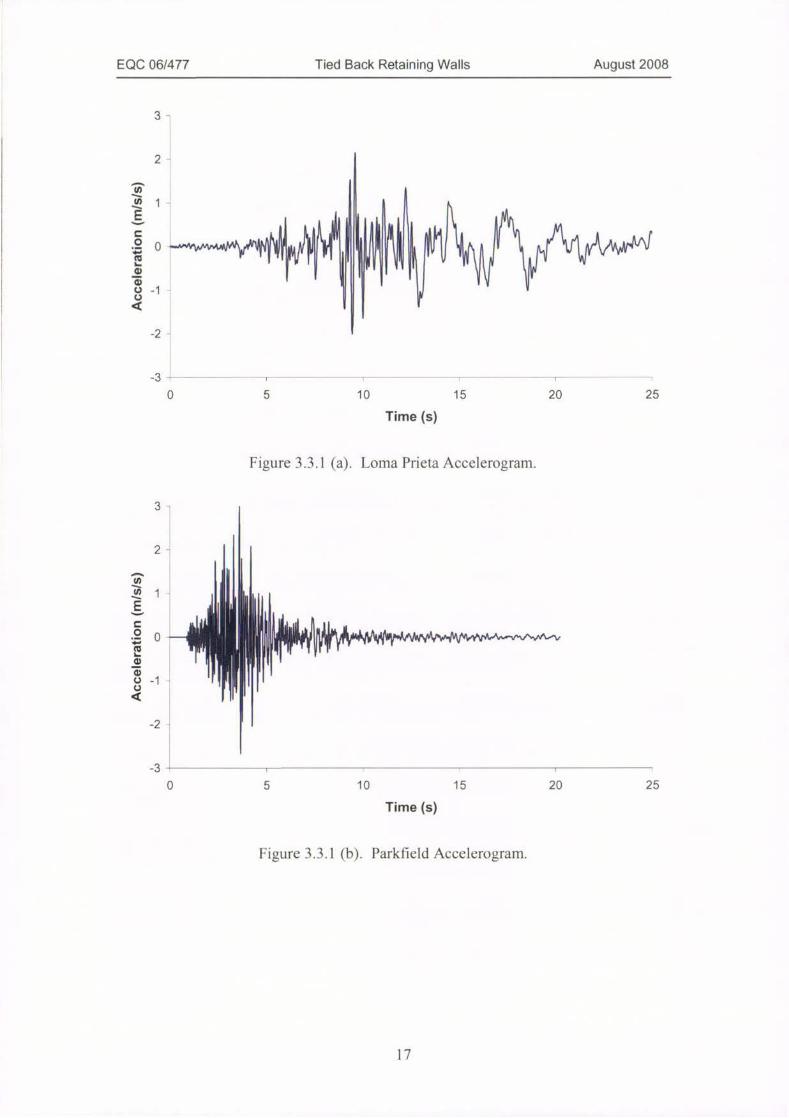
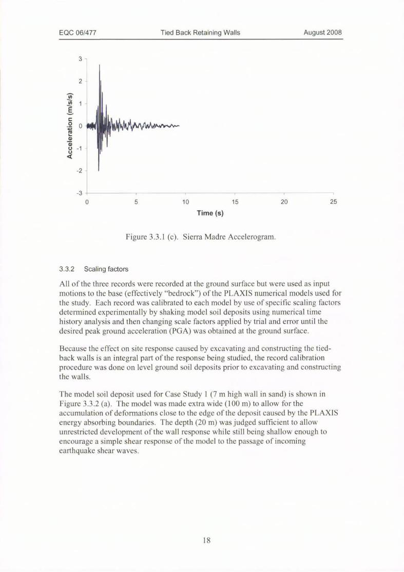
All three records (shown in Figures 3.3.1 (a), (b), and (c)) are characterised by
relatively modest values of PGA but they have a useful range of magnitudes for thesort o f event that usually shows up in the de-aggregation of site specific hazard
studies. The Sierra Madre record comes from a low magnitude and is characterised
by a single strong pulse and some low level high freq noise. The Loma Prieta recordcorresponds to a larger magnitude and it contains several significant cycles of shakingbut with lower PGA due to the greater distance. The Parkfield record is in-between:
moderate magnitude, small distance, larger PGA, several cycles.
16
EQC 06/477 Tied Back Retaining Walls August 2008
3-
2-
1
0-1
-1 -
-2 -
-3
Time (s)
0 5 10 15 20 25
Figure 3.3.1 (a). I oma Prieta Accelerogram.
3
2-
1
-1
-2 -
-3
0 5 10
#Af#,44901*vy.&-vv-
15 20 25
Time (s)
Figure 3.3.1 (b). Parkfield Accelerogram.
17
EQC 06/477 Tied Back Retaining Walls August 2008
3-
2-
1
0
G
G
i -1-2
-3
0 5 10 15 20 25
Time (s)
Figure 3.3.1 (c). Sierra Madre Accelerogram.
3.3.2 Scaling factors
All o f the three records were recorded at the ground surface but were used as inputmotions to the base (effectively "bedrock") of the PLAXIS numerical models used forthe study. Each record was calibrated to each model by use of specific scaling factorsdetermined experimentally by shaking model soil deposits using numerical timehistory analysis and then changing scale factors applied by trial and error until thedesired peak ground acceleration ( PGA) was obtained at the ground surface.
Because the effect on site response caused by excavating and constructing the tied-back walls is an integral part of the response being studied, the record calibrationprocedure was done on level ground soil deposits prior to excavating and constructingthe walls.
The model soil deposit used for Case Study 1 (7 m high wall in sand) is shown inFigure 3.3.2 (a). The model was made extra wide (100 m) to allow for theaccumulation of deformations close to the edge of the deposit caused by the PLAXISenergy absorbing boundaries. The depth (20 m) was judged sufficient to allowunrestricted development ofthe wall response while still being shallow enough toencourage a simple shear response of the model to the passage of incomingearthquake shear waves.
18
EQC 06/477 Tied Back Retaining Walls August 2008
0.00 10.00 20.00 30.00 .0.00 50.00 60.00 70.00 80.00 90.00 100.00
30,00 -
10·22
ly Lt-+
44 +1 14 ++,0.921= 5353*3 55505 )*
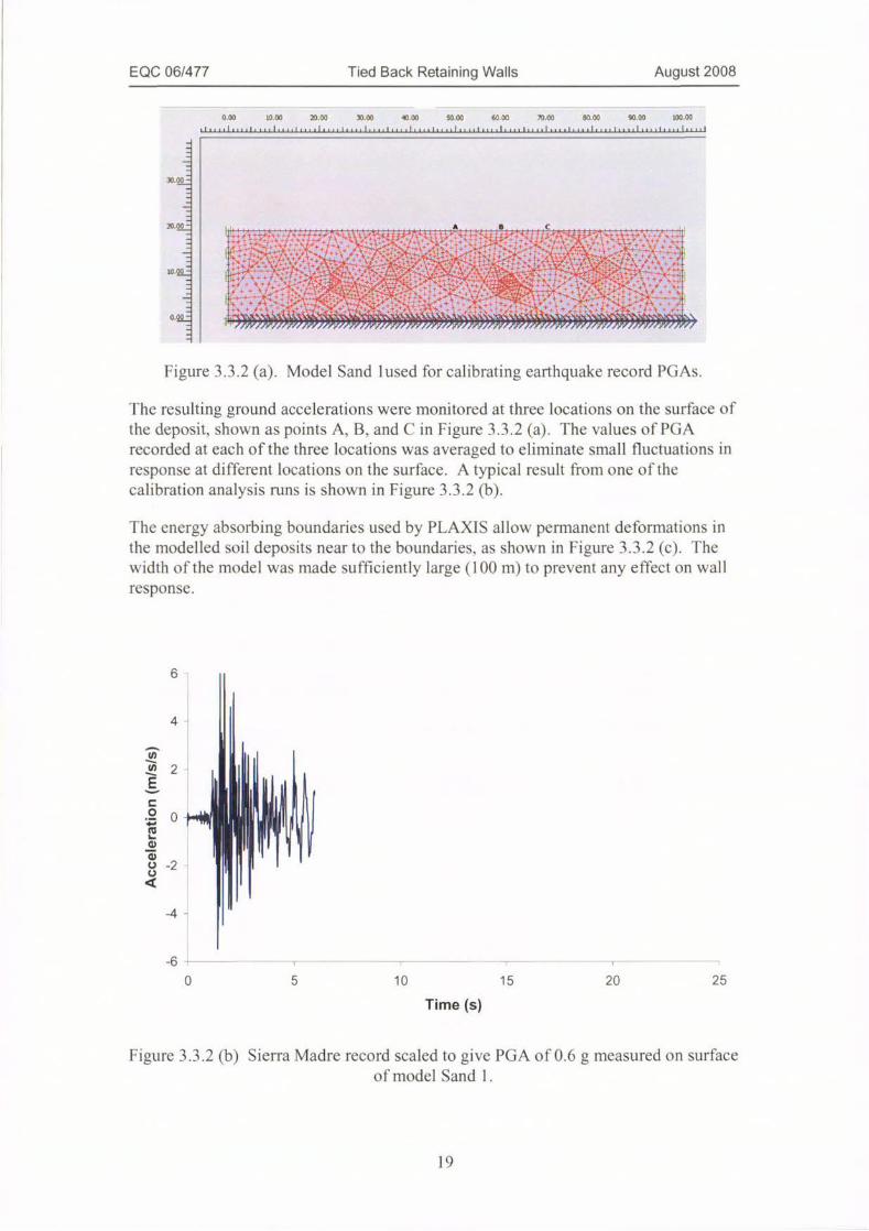
Figure 3.3.2 (a). Model Sand lused for calibrating earthquake record PGAs.
The resulting ground accelerations were monitored at three locations on the surface ofthe deposit, shown as points A, B, and C in Figure 3.3.2 (a). The values of PGArecorded at each of the three locations was averaged to eliminate small fluctuations inresponse at different locations on the surface. A typical result from one of thecalibration analysis runs is shown in Figure 3.3.2 (b).
The energy absorbing boundaries used by PLAXIS allow permanent deformations inthe modelled soil deposits near to the boundaries. as shown in Figure 3.3.2 (c). The
width ofthe model was made sufficiently large (100 m) to prevent any effect on wallresponse.
6
4-
5 2
2 -2 -
-4 -
-6
0 5 10 15 20 25
Time (s)
Figure 3.3.2 (b) Sierra Madre record scaled to give PGA of 0.6 g measured on surfaceof model Sand 1.
19

EQC 06/477 Tied Back Retaining Walls August 2008
0.00 10.00 20.00 30.00 40.00 50.00 60.00 70.00 80.00 90.00 100.00
i,1.,i,1.,i,1.,i,]ii,il,i.ilii.,ti.,il...il,i.,lii.,Ii,i,1.'.il,i''lii,ili.,ilii.,Ii.,il,i"Ii,"Iii"Ii,ill,1
30.00 -
20.00 -
10.00 -
°4 :p#>**Iti*;*4*46)@*tkkd .ri
Figure 3.3.2 (c) Model Sand 1 after earthquake shaking.
1-he resulting scaling factors determined for model Sand 1 are shown in Table 3.3.2(a) for the three different values of surface PGA selected for use in the study. The
scaling factors do not represent a linear relationship between scaled base input recordand surface PGA: The scaling factors increase markedly with increasing targetsurface PGA, presumably because of increasing soil non-linearity effects.
Table 3.3.2 (a). Scaling factors determined for model Sand 1.
Earthquake Record Target PGA
0.2 g 0.4 g 0.6 g
Loma Prieta 0.22 0.53 0.97
Parkfield 0.22 0.46 0.77
Sierra Madre 0.30 0.69 1.11
For Case Study 2 and 3 (12 In high wall in sand) the depth of the soil deposit wasincreased to 25 in to maintain the same depth of soil beneath the excavation. Thescaling factors for this soil deposit (Table 3.3.2 (b)) were slightly different frommodel Sand 1 because ofthe increased thickness of the soil deposit. Scale factorswere only determined for the I.oma Prieta record because this was found to give byfar the greatest wall deformation response for ('ase Study 1
Table 3.3.2 (2). Scaling factors determined for niodel Sand 2 and Sand 3
Earthquake Record Target PGA
0.2 g 0.4 g 0.6 g
Loma Prieta 0.28 0.60 1.0
20
EQC 06/477 Tied Back Retaining Walls August 2008
3.4 Case Study 1: Single Row of Anchors in Sand
3.4.1 Case study description
This case is for a 7 ni deep excavation in sand. It is assumed that the water table hasbeen drawn down to the base ofthe excavation. Typically, such an excavation wouldbe made using concrete soldier piles with sprayed concrete facing for a permanentinstallation or galvanised steel UC sections with timber lagging. A single row of tie-back ground anchors is usually found to provide an economical solution with a twostage excavation process: Installation of soldier piles from the ground surface,excavation to 2 m depth. installation and stressing of the ground anchors, and finalexcavation to full depth.
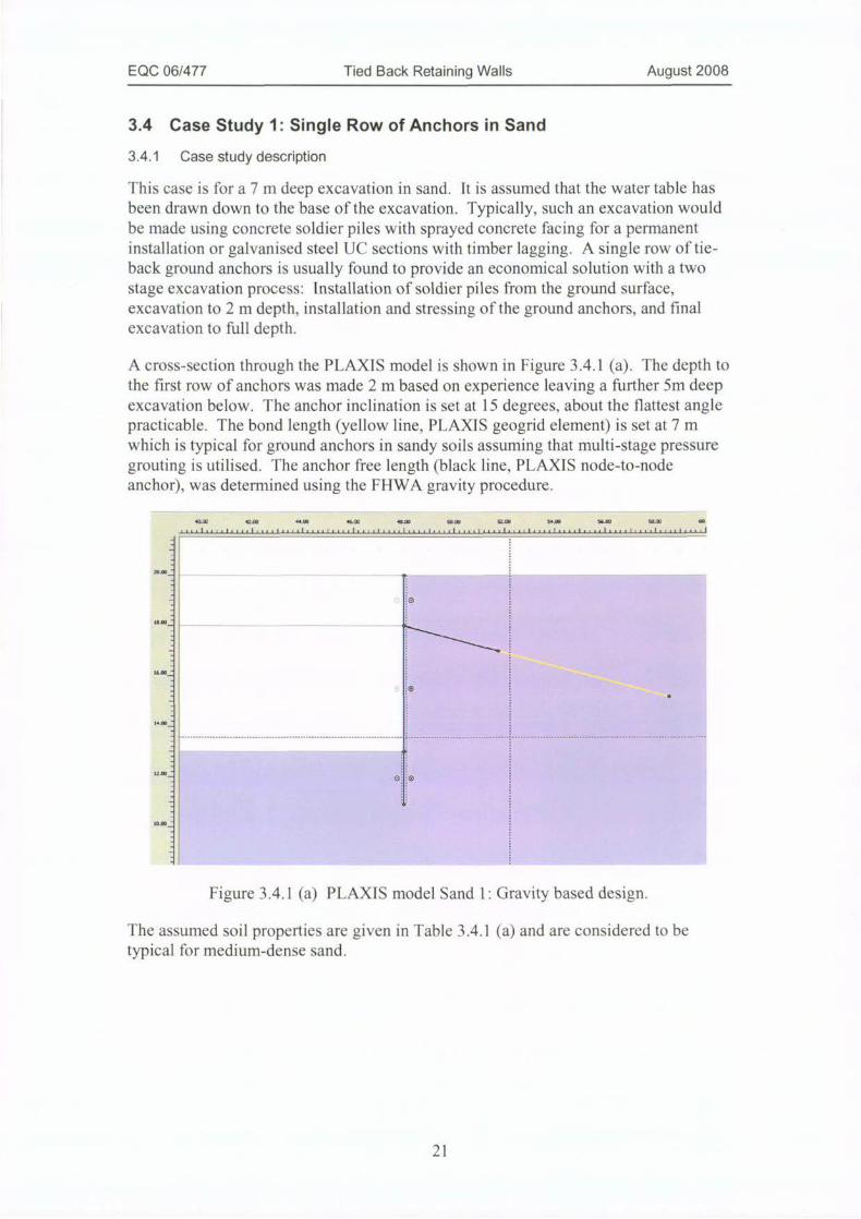
A cross-section through the PLAXIS model is shown in Figure 3.4.1 (a). The depth tothe first row of anchors was made 2 m based on experience leaving a further 5m deepexcavation below. The anchor inclination is set at 15 degrees, about the flattest anglepracticable. The bond length (yellow line, PLAXIS geogrid element) is set at 7 mwhich is typical for ground anchors in sandy soils assuming that multi-stage pressuregrouting is utilised. The anchor free length (black line. PLAXIS node-to-nodeanchor), was determined using the FHWA gravity procedure.
U - I. - - - - - - U .
0
14.00
120.-
10.00
Figure 3.4.1 (a) PLAXIS model Sand 1: Gravity based design.
The assumed soil properties are given in Table 3.4.1 (a) and are considered to betypical for medium-dense sand.
21

EQC 06/477 Tied Back Retaining Walls August 2008
Table 3.4.1 (a) Soil properties for case studies in sand.
Property Symbol Value
Density, unsaturated yunsat16 KN/m3
Density, saturated ysat 18 KN/m3
Effective cohesion c' 1 KN/m2
Effective friction 0 35 degrees
Soil model Hardening soil
Young's Modulus E5lref 30 MN/m3
Young's Modulus Euref(unload/reload)
90 MN/m3
3.4.2 Case la: Gravity design
Gravity design followed the FHWA gravity procedure described in Section 2.2.2.
Detailed calculations are given in Appendix A and are summarised in Table 3.4.2 (a).
Table 3.4.2 (a). Design values for case study Sand la: Gravity design.
Design Parameter Value
Apparent earth pressure, p 30 KN/m2
Anchor design load (horizontal) 108 KN/m
Base reaction 30 KN/m
Negative bending moment (at anchor) 28 KNm/m
Maximum bending moment (below anchor) 45 KNm/m
ULS design bending moment, M* 72 KNm/m
The wall structural elements were designed using these basic calculated design values
with details given in Iable 3.4.2 (b). Forthe purposes of this research project, designsolutions were perfectly optimised. whereas for everyday design it would be
necessary to select from standard products (e.g. standard anchor configurations. stocksteel sections. etc.).
22
EQC 06/477 Tied Back Retaining Walls August 2008
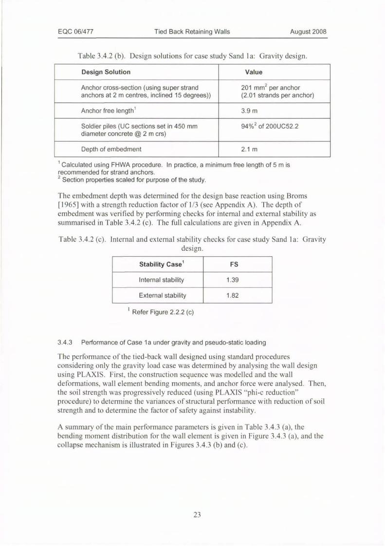
Table 3.4.2 (b). Design solutions for case study Sand 1 a: Gravity design.
Design Solution Value
Anchor cross-section (using super strandanchors at 2 m centres, inclined 15 degrees))
201 mm2 per anchor(2.01 strands per anchor)
Anchor free lengthl 3.9 m
Soldier piles (UC sections set in 450 mm 94%2 of 200UC52.2
diameter concrete @2m crs)
Depth of embedment 2.1 m
1 Calculated using FHWA procedure. In practice, a minimum free length of 5 m isrecommended for strand anchors.
2 Section properties scaled for purpose of the study.
The embedment depth was determined for the design base reaction using Broms
[1965] with a strength reduction factor of 1 /3 (see Appendix A). The depth ofembedment was verified by performing checks for internal and external stability as
summarised in Table 3.4.2 (c). The full calculations are given in Appendix A.
1 able 3.4.2 (c). Internal and external stability checks for case study Sand 1 a: Gravitydesign.
Stability Casel FS
Internal stability 1.39
External stability 1.82
1 Refer Figure 2.2.2 (c)
3.4.3 Performance of Case 1 a under gravity and pseudo-static loading
The performance of the tied-back wall designed using standard proceduresconsidering only the gravity load case was determined by analysing the wall designusing PLAXIS. First, the construction sequence was modelled and the walldeformations. wall element bending moments. and anchor force were analysed. Then.
the soil strength was progressively reduced (using PLAXIS "phi-c reduction"procedure) to determine the variances of structural performance with reduction ofsoil
strength and to determine the factor of safety against instability.
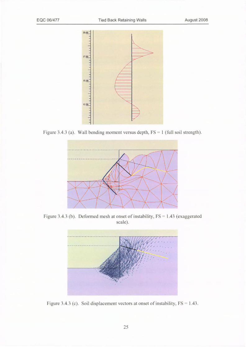
A summary ofthe main performance paranieters is given in Table 3.4.3 (a), thebending moment distribution for the wall element is given in Figure 3.4.3 (a), and the
collapse mechanism is illustrated in Figures 3.4.3 (b) and (c).
23
EQC 06/477 Tied Back Retaining Walls August 2008
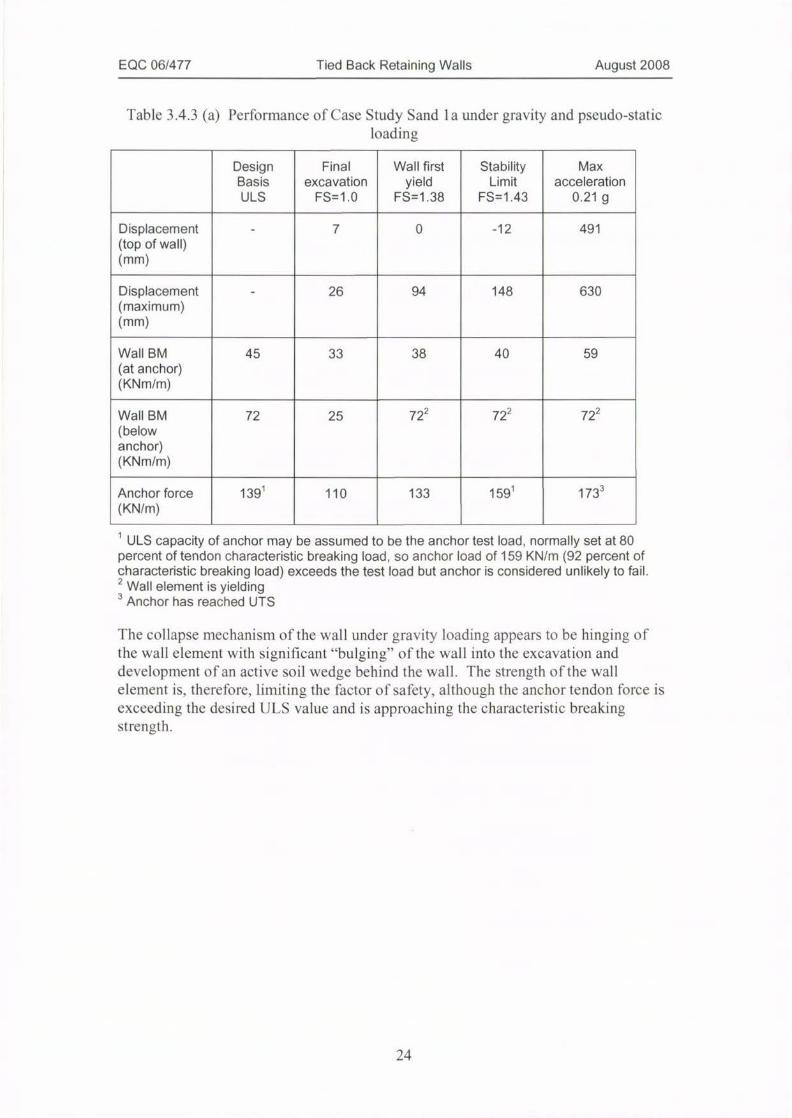
Table 3.4.3 (a) Performance of Case Study Sand 1 a under gravity and pseudo-static
loading
Design Final Wai I first Stability Max
Basis excavation yield Limit acceleration
ULS FS=1.0 FS=1.38 FS=1.43 0.21 g
Displacement - 7 0 -12 491
(top of wall)(mm)
Displacement - 26 94 148 630
(maximum)(mm)
Wall BM 45 33 38 40 59
(at anchor)(KNm/m)
Wall BM 72 25 722 722 72(belowanchor)(KNm/m)
2
Anchor force 139
(KN/m)
1110 133 1591 173
3
1
ULS capacity of anchor may be assumed to be the anchor test load, normally set at 80percent of tendon characteristic breaking load, so anchor load of 159 KN/m (92 percent ofcharacteristic breaking load) exceeds the test load but anchor is considered unlikely to fail.2 Wall element is yielding3 Anchor has reached UTS
The collapse mechanism of the wall under gravity loading appears to be hinging ofthe wall element with significant "bulging" of the wall into the excavation anddevelopment of an active soil wedge behind the wall. The strength ofthe wallelement is, therefore, limiting the factor of safety, although the anchor tendon force isexceeding the desired 1JLS value and is approaching the characteristic breakingstrength.
24
EQC 06/477 Tied Back Retaining Walls August 2008
20.8-
17.0
15./L
12.50
Figure 3.4.3 (a). Wall bending moment versus depth, FS = 1 (full soil strength).
•1./ DE-lul-0 - -79=4Figure 3.4.3 (b). Deformed mesh at onset of instability, FS = 1.43 (exaggerated
scale).
A
Figure 3.4.3 (c). Soil displacement vectors at onset of instability. FS = 1.43.
25

EQC 06/477 Tied Back Retaining Walls August 2008
t:u=rUu*:UU U -++
4
Figure 3.4.3 (d). Soil displacement countours at onset of instability. pseudo-staticacceleration = 0.21 g
Under pseudo-static acceleration of 0.21 g, the wall is undergoing external stabilityfailure (Figure 3.4.3 (d)) at about the same time as the anchor force reaches materialultimate tensile strength.
3.4.4 Evaluation of Case la under gravity loading
The factor of safety achieved in the PLAXIS analysis using "phi-c reduction" (lowerbound) is considered satisfactory. Typically, acceptable factors of safety for slopestability analyses using limiting equilibrium methods of analysis (upper bound) areconsidered to be in the range from FS = 1.2 to FS = 1.5 for critical slopes.
1 he factor of safety determined for this case study (FS = 1.43) is close to the value
calculated using the "by hand" limiting equilibrium procedure (internal stability, FS =1.39).
The PLAXIS analysis suggests that it may be possible to improve the factor of safetyby increasing the yield bending strength of the wall. However, experience shows thatincreasing the bending strength of the wall gives little improvement once the soilactive wedge has developed.
1-he capacity of the wall under pseudo-static loading is surprisingly good, with failureoccurring along the desirable external stability mechanism. The anchor forceincreases to reach UTS as displacements increase. but only after very large walltranslational displacements are achieved (greater than 600 mni).
3.4.5 Performance of gravity design Case la under seismic loading
Ihe performance of the gravity design Linder seismic loading was determined byapplying the suite ofthree scaled earthquake time-history records to the PLAXIS
model over a range ofincreasing PGA's: 0.2 g, 0.4 g, and 0.6 g.
Wall performance is indicated primarily by outwards permanent displacement"
remaining after each earthquake "event . For walls with a single row of tie-back
26
EQC 06/477 Tied Back Retaining Walls August 2008
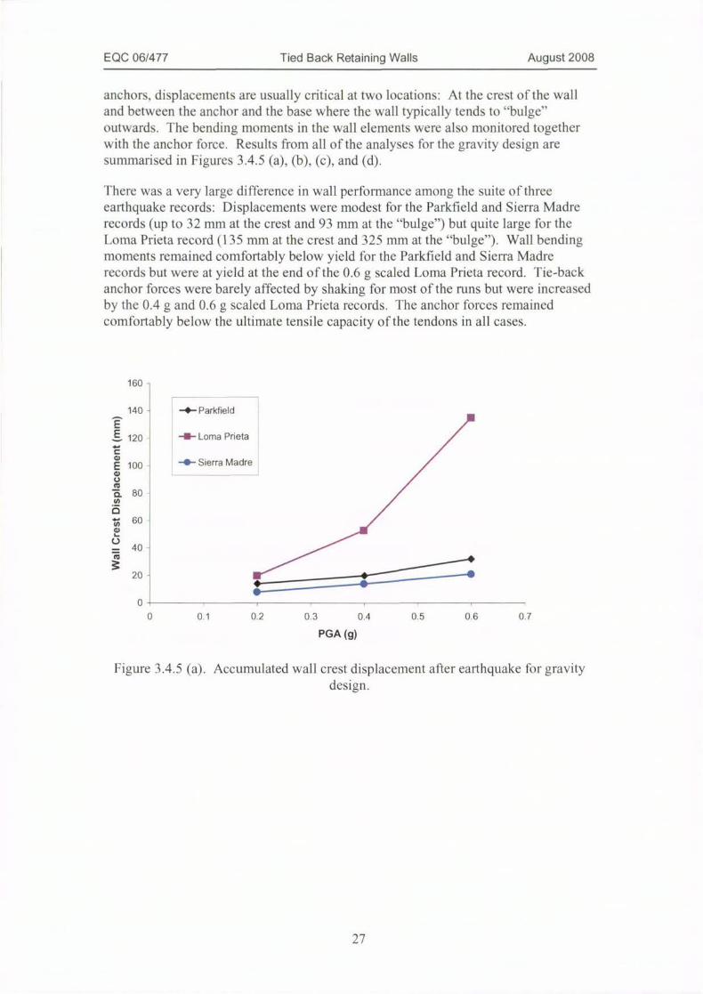
anchors, displacements are usually critical at two locations: At the crest of the walland between the anchor and the base where the wall typically tends to "bulge"
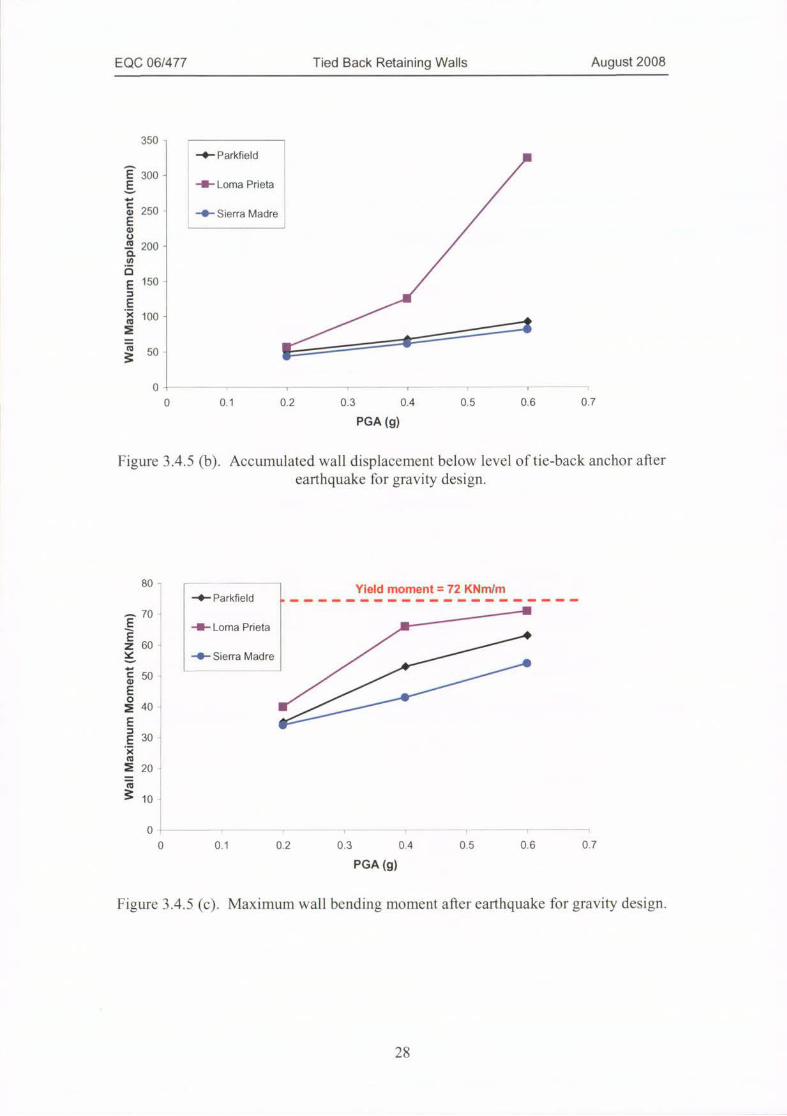
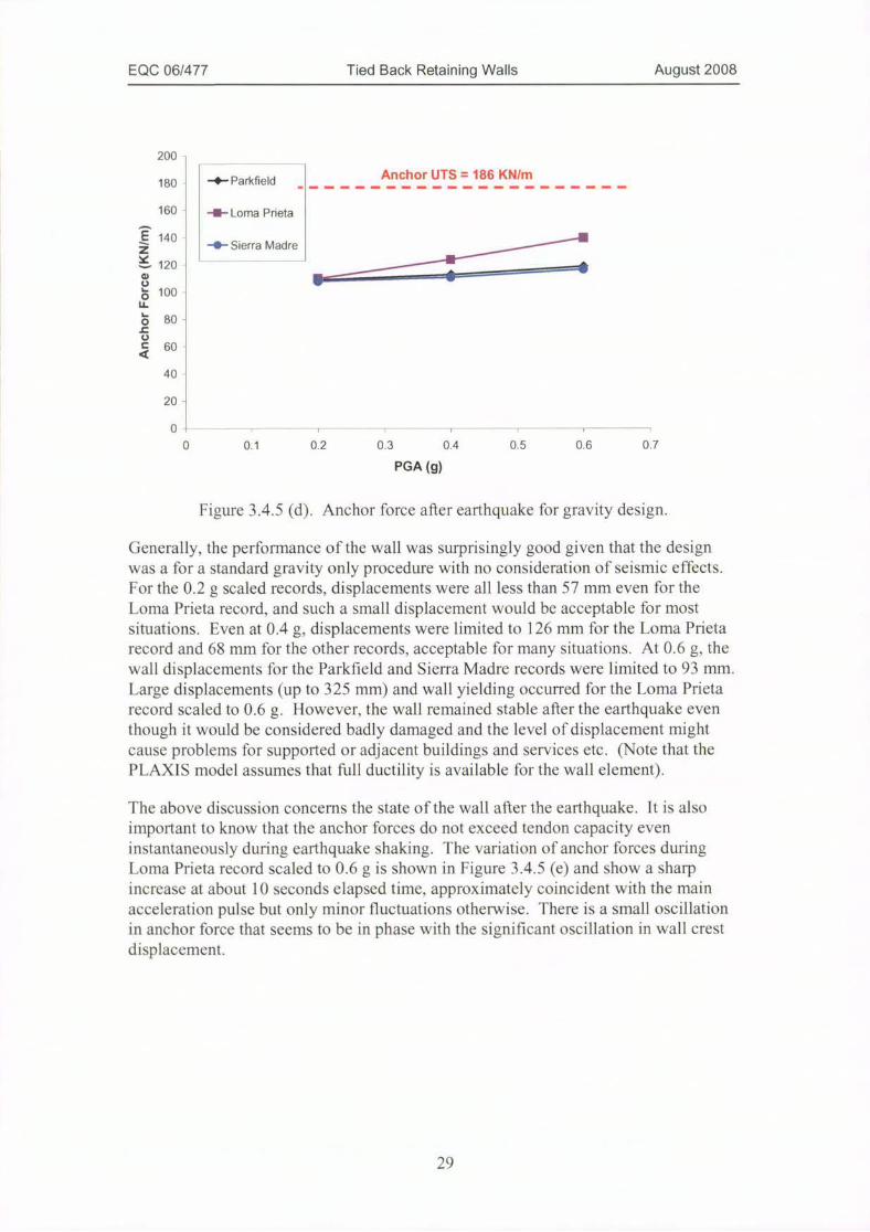
outwards. The bending moments in the wall elements were also monitored togetherwith the anchor force. Results from all ofthe analyses for the gravity design are
summarised in Figures 3.4.5 (a), (b), (c), and (d).
There was a very large difference in wall performance among the suite of threeearthquake records: Displacements were modest for the Parkfield and Sierra Madre
records (up to 32 mm at the crest and 93 mm at the "bulge") but quite large for theLoma Prieta record (135 mm at the crest and 325 mm at the "bulge"). Wall bendingmoments remained comfortably below yield for the Parkfield and Sierra Madre
records but were at yield at the end ofthe 0.6 g scaled Loma Prieta record. Tie-backanchor forces were barely affected by shaking for most of the runs but were increasedby the 0.4 g and 0.6 g scaled Loma Prieta records. The anchor forces remainedcomfortably below the ultimate tensile capacity ofthe tendons in all cases.
160 -
140 - , -0- Parkfield
. 120 - -il-Loma Prieta
-O- Sierra Madre
80
60
40
20 -
0
0 0.1 0.2 0.3 0.4 0.5 0.6 0.7
PGA (g)
Figure 3.4.5 (a). Accumulated wall crest displacement after earthquake fur gravitydesign.
27
EQC 06/477 Tied Back Retaining Walls August 2008
350 -
-0- Parkfield
-il-Loma Prieta
250 -0- Sierra Madre
200 -
150
100 - Mkzz /-==150
0 1 1 1 1 1 1 1
0 0.1 0.2 0.3 0.4 0.5 0.6 0.7
PGA (g)
Figure 3.4.5 (b). Accumulated wall displacement below level of tie-back anchor afterearthquake for gravity design.
80 -Yield moment = 72 KNm/m
-0- Parkfield ..
. 70- ,---1-il-Loma Prieta B-
60 -
-O- Sierra Madre
50 -
40
30 -
20 -
10 -
0
0 0.1 0.2 0.3 0.4 0.5 0.6 0.7
PGA (g)
Figure 3.4.5 (c). Maximum wall bending moment after earthquake for gravity design.
28
EQC 06/477 Tied Back Retaining Walls August 2008
200 -
Anchor UTS = 186 KN/m180 -+- Parkfield
.---------------------
160 - -li-Loma Prieta
140-O- Sierra Made
2 120
100
80 -
60
40
20 -
0
0 0.1 0.2 0.3 0.4 0.5 0.6 0.7
PGA (g)
Figure 3.4.5 (d). Anchor force after earthquake for gravity design.
Generally, the performance of the wall was surprisingly good given that the designwas a for a standard gravity only procedure with no consideration of seismic effects.For the 0.2 g scaled records. displacements were all less than 57 mm even for theLoma Prieta record. and such a small displacement would be acceptable for mostsituations. Even at 0.4 g, displacements were limited to 126 mm for the Loma Prietarecord and 68 mill for the other records, acceptable for many situations. At 0.6 g. thewall displacements for the Parkfield and Sierra Madre records were limited to 93 mm.Large displacements (up to 325 mm) and wall yielding occurred for the Loma Prietarecord scaled to 0.6 g. However. the wall remained stable after the earthquake eventhough it would be considered badly damaged and the level ofdisplacement mightcause problems for supported or adjacent buildings and services etc. (Note that thePLAXIS model assumes that full ductility is available for the wall element).
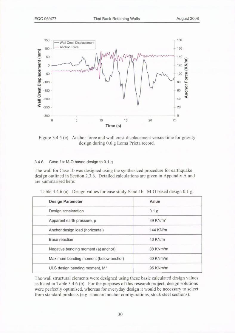
The above discussion concerns the state of the wall after the earthquake. It is alsoimportant to know that the anchor forces do not exceed tendon capacity eveninstantaneously during earthquake shaking. The variation of anchor forces duringLoma Prieta record scaled to 0.6 g is shown in Figure 3.4.5 (e) and show a sharpincrease at about 10 seconds elapsed time, approximately coincident with the mainacceleration pulse but only minor fluctuations otherwise. There is a small oscillationin anchor force that seems to be in phase with the significant oscillation in wall crestdisplacement.
29
EQC 06/477 Tied Back Retaining Walls August 2008
150
100
-Wall Crest Displacement
- Anchor Force
- 180
- 160
E. 50 - A A Wifl A\'#A. -- 140 -I E
-
- 120 Z
* -50 74 - 100 8»/ b
2 -100 - - 80 U.
-150 - -607 5) LJ-200 - -40
0mc
64
-250 - - 20
-300 0
0 5 10 15 20 25
Time (s)
Figure 3.4.5 (e). Anchor force and wall crest displacement versus time for gravitydesign during 0.6 g Loma Prieta record.
Case lb: M-O based design to 0.1 g
The wall for Case lb was designed using the synthesized procedure for earthquakedesign outlined in Section 2.3.6. Detailed calculations are given in Appendix A andare summarised here:
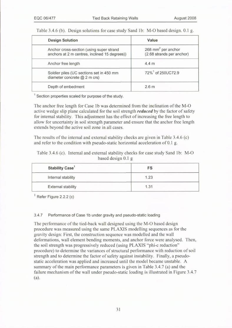
Table 3.4.6 (a). Design values for case study Sand 1 b: M-O based design 0.1 g.
Design Parameter Value
Design acceleration 0.1 g
Apparent earth pressure, p 39 KN/m2
Anchor design load (horizontal) 144 KN/m
Base reaction 40 KN/m
Negative bending moment (at anchor) 38 KNm/m
Maximum bending moment (below anchor) 60 KNm/m
ULS design bending moment, M* 95 KNm/m
The wall structural elements were designed using these basic calculated design valuesas listed in Table 3.4.6 (b). For the purposes of this research project, design solutionswere perfectly optimised, whereas for everyday design it would be necessary to selectfrom standard products (e.g. standard anchor configurations, stock steel sections).
30
EQC 06/477 Tied Back Retaining Walls August 2008
Table 3.4.6 (b). Design solutions for case study Sand lb: M-0 based design. 0.1 g.
Design Solution Value
Anchor cross-section (using super strand
anchors at 2 m centres, inclined 15 degrees))268 mm2 per anchor(2.68 stands per anchor)
Anchor free length 4.4 m
Soldier piles (UC sections set in 450 mm 72%
diameter concrete @2m crs)
1of 250UC72.9
Depth of embedment 2.6 m
1 Section properties scaled for purpose of the study.
The anchor free length for Case lb was determined from the inclination of the M-0active wedge slip plane calculated for the soil strength reduced by the factor of safetyfor internal stability. This adjustment has the effect of increasing the free length toallow for uncertainty in soil strength parameter and ensure that the anchor free length
extends beyond the active soil zone in all cases.
The results ofthe internal and external stability checks are given in Table 3.4.6 (c)and re fur to the condition with pseudo-static horizontal acceleration of 0.1 g.
Table 3.4.6 (c). Internal and external stability checks for case study Sand l b: M-0based design 0.1 g
1
Stability Casel FS
Internal stability 1.23
External stability 1.31
Refer Figure 2.2.2 (c)
3.4.7 Performance of Case 1 b under gravity and pseudo-static loading
The performance o f the tied-back wall designed using the M-0 based designprocedure was measured using the same PLAXIS modelling sequences as for thegravity design: First, the construction sequence was modelled and the walldeformations, wall element bending moments, and anchor force were analysed. Then,the soil strength was progressively reduced (using PLAXIS "phi-c reduction"procedure) to determine the variances of structural performance with reduction of soilstrength and to determine the factor of safety against instability. Finally, a pseudo-static acceleration was applied and increased until the model became unstable. Asummary of the main performance parameters is given in Table 3.4.7 (a) and thefailure mechanism of the wall under pseudo-static loading is illustrated in Figure 3.4.7(a).
31
EQC 06/477 Tied Back Retaining Walls August 2008
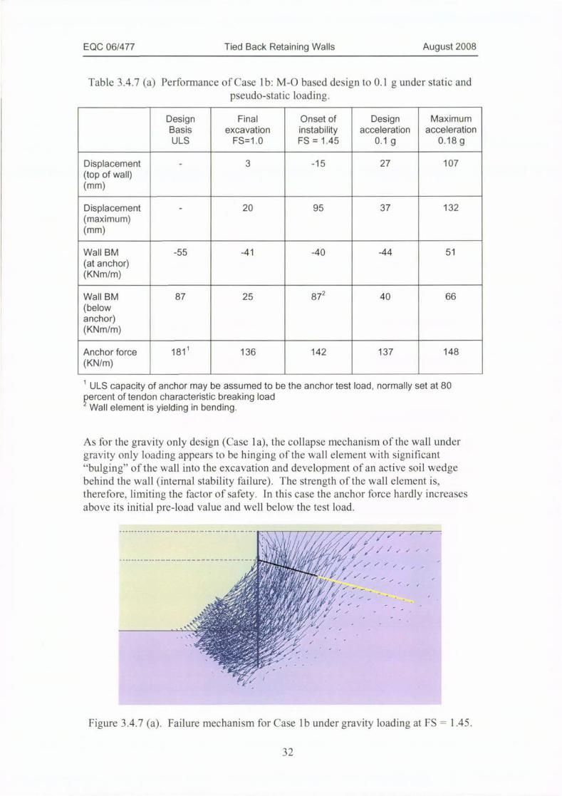
Table 3.4.7 (a) Performance ofCase lb: M-O based design to 0.1 g under static andpseudo-static loading.
Design Final Onset of Design Maximum
Basis excavation instability acceleration acceleration
ULS FS=1.0 FS = 1.45 0.1 g 0.18g
Displacement - 3 -15 27 107(top of wall)(mm)
Displacement - 20 95 37 132(maximum)(mm)
Wall BM -55 -41 -40 -44 51
Cat anchor)(KNm/m)
Wall BM 87 25 87
(belowanchor)
(KNm/m)
2 40 66
Anchor force 181
(KN/m)
1136 142 137 148
1 ULS capacity of anchor may be assumed to be the anchor test load, normally set at 80
percent of tendon characteristic breaking loadWall element is yielding in bending.
As for the gravity only design (Case la), the collapse mechanism of the wall undergravity only loading appears to be hinging of the wall element with significant"bulging" of the wall into the excavation and development of an active soil wedgebehind the wall (internal stability failure). The strength of the wall element is,therefore, limiting the factor of safety. In this case the anchor force hardly increasesabove its initial pre-load value and well below the test load.
*589¥4;>64/491 .
Figure 3.4.7 (a). Failure mechanism for Case 1 b under gravity loading at FS = 1.45.
32
EQC 06/477 Tied Back Retaining Walls August 2008
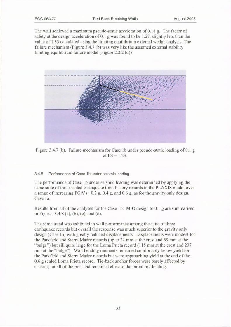
The wall achieved a maximum pseudo-static acceleration of 0.18 g. The factor of
safety at the design acceleration of 0.1 g was found to be 1.27, slightly less than the
value of 1.33 calculated using the limiting equilibrium external wedge analysis. The
failure mechanism (Figure 3.4.7 (b) was very like the assumed external stability
limiting equilibrium failure model (Figure 2.2.2 (d))
Figure 3.4.7 (b). Failure mechanism for Case 1 b under pseudo-static loading of 0.1 gat FS = 1.23.
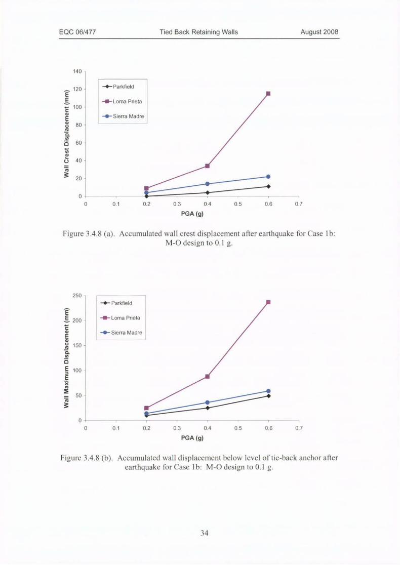
3.4.8 Performance of Case 1 b under seismic loading
The performance of Case 1 b under seismic loading was determined by applying thesame suite of three scaled earthquake time-history records to the PLAXIS model over
a range of increasing PGA's: 0.2 g. 0.4 g, and 0.6 g. as for the gravity only design,Case 1 a.
Results from all of the analyses for the Case 1 b: M-O design to 0.1 g are summarised
in Figures 3.4.8 (a), (b), (c).and (d).
The same trend was exhibited in wall performance among the suite ofthree
earthquake records but overall the response was much superior to the gravity only
design (Case la) with greatly reduced displacements: Displacements were modest forthe Parkfield and Sierra Madre records (up to 22 mm at the crest and 59 mm at the
"bulge") but sill quite large for the Loma Prieta record (115 min at the crest and 237
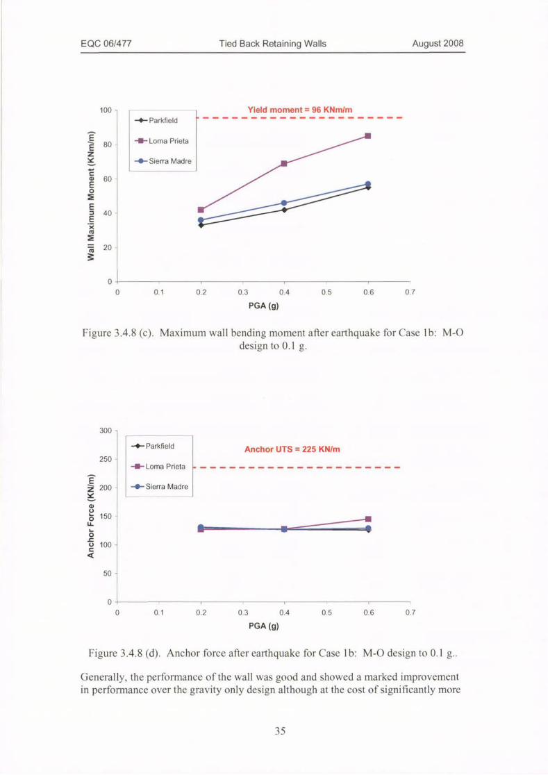
nim at the "bulge"). Wall bending moments remained comfortably below yield for
the Parkfield and Sierra Madre records but were approaching yield at the end of the
0.6 g scaled Loma Prieta record. Tie-back anchor forces were barely affected by
shaking for all ofthe runs and remained close to the initial pre-loading.
33
EQC 06/477 Tied Back Retaining Walls August 2008
140 -
120 --0- Parkfield
,-#I- Loma Prieta
100 -
-O- Sierra Madre
80 -
60 -
40 -
20 - -0
0 i ----- ----r- i, 1
0 0.1 0.2 0.3 0.4 0.5 0.6 0.7
PGA (g)
Figure 3.4.8 (a). Accumulated wall crest displacement after earthquake for Case 1 b:M-O design to 0.1 g.
250 -
-0- Parkfield
. 200 --- Loma Prieta
-O- Sierra Made
150 -
100
50
A=Z=0
0 0.1 0.2 0.3 0.4 0.5 0.6 0.7
PGA (g)
Figure 3.4.8 (b). Accumulated wall displacement below level of tie-back anchor afterearthquake for Case lb: M-0 design to 0.1 g.
34
EQC 06/477 Tied Back Retaining Walls August 2008
100 - Yield moment = 96 KNm/m
-0- Parkfield
80 --m- Loma Prieta
4- Sierra Madre B-
60 -
40 - GESS=20
0
0 0.1 0.2 0.3 0.4 0.5 0.6 0.7
PGA (g)
Figure 3.4.8 (c). Maximum wall bending moment after earthquake for Case 1 b: M-Odesign to 0.1 g.
300 -
--ParkfieldAnchor UTS = 225 KN/m
250 --I- Loma Prieta - - -------- ------------
200 - -f Sierra Madre
150
.
100 -
50 -
0
0 0.1 0.2 0.3 0.4 0.5 0.6 0.7
PGA (g)
Figure 3.4.8 (d). Anchor force after earthquake for Case 1 b: M-O design to 0.1 g..
Generally, the performance of the wall was good and showed a marked improvementin performance over the gravity only design although at the cost of significantly more
35
EQC 06/477 Tied Back Retaining Walls August 2008
materials in both wall elements and anchors. A more detailed comparison among allthe design cases is given in Section 3.4.18.
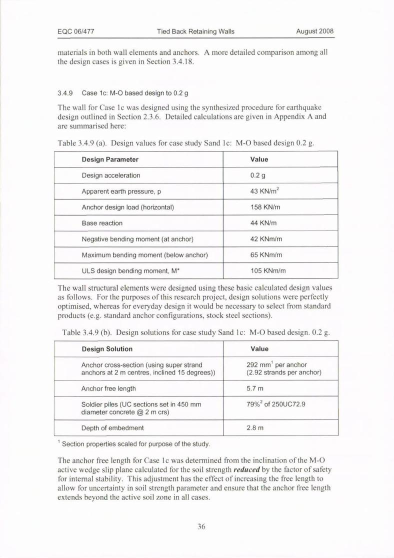
3.4.9 Case lc: M-O based design to 0.2 g
The wall for Case 1 c was designed using the synthesized procedure for earthquakedesign outlined in Section 2.3.6. Detailed calculations are given in Appendix A andare summarised here:
Table 3.4.9 (a). Design values for case study Sand le: M-O based design 0.2 g.
Design Parameter Value
Design acceleration 0.2 g
Apparent earth pressure, p 43 KN/m2
Anchor design load (horizontal) 158 KN/m
Base reaction 44 KN/m
Negative bending moment (at anchor) 42 KNm/m
Maximum bending moment (below anchor) 65 KNm/m
ULS design bending moment, M* 105 KNm/m
The wall structural elements were designed using these basic calculated design valuesas follows. For the purposes of this research project, design solutions were perfectlyoptimised, whereas for everyday design it would be necessary to select from standardproducts (e.g. standard anchor configurations, stock steel sections).
Table 3.4.9 (b). Design solutions for case study Sand 1 c: M-O based design. 0.2 g.
Design Solution Value
Anchor cross-section (using super strandanchors at 2 m centres, inclined 15 degrees))
292 mrnl per anchor(2.92 stands per anchor)
Anchor free length 5.7 m
Soldier piles (UC sections set in 450 mm 79%
diameter concrete @2m crs)
2 of 250UC72.9
Depth of embedment 2.8 m
1 Section properties scaled for purpose of the study.
The anchor free length for Case 1 c was determined from the inclination of the M-0active wedge slip plane calculated for the soil strength reduced by the factor o f safetyfor internal stability. This adjustment has the effect of increasing the free length toallow for uncertainty in soil strength parameter and ensure that the anchor free lengthextends beyond the active soil zone in all cases.
36
EQC 06/477 Tied Back Retaining Walls August 2008
The results ofthe internal and external stability checks are given in Table 3.4.9 (c)and refur to the condition with pseudo-static horizontal acceleration of 0.2 g.
Table 3.4.9 (c). Internal and external stability checks for case study Sand 1 c: M-0based design 0.2 g
1
Stability Casel FS
Internal stability 1.25
External stability 1.16
Refer Figure 2.2.2 (c)
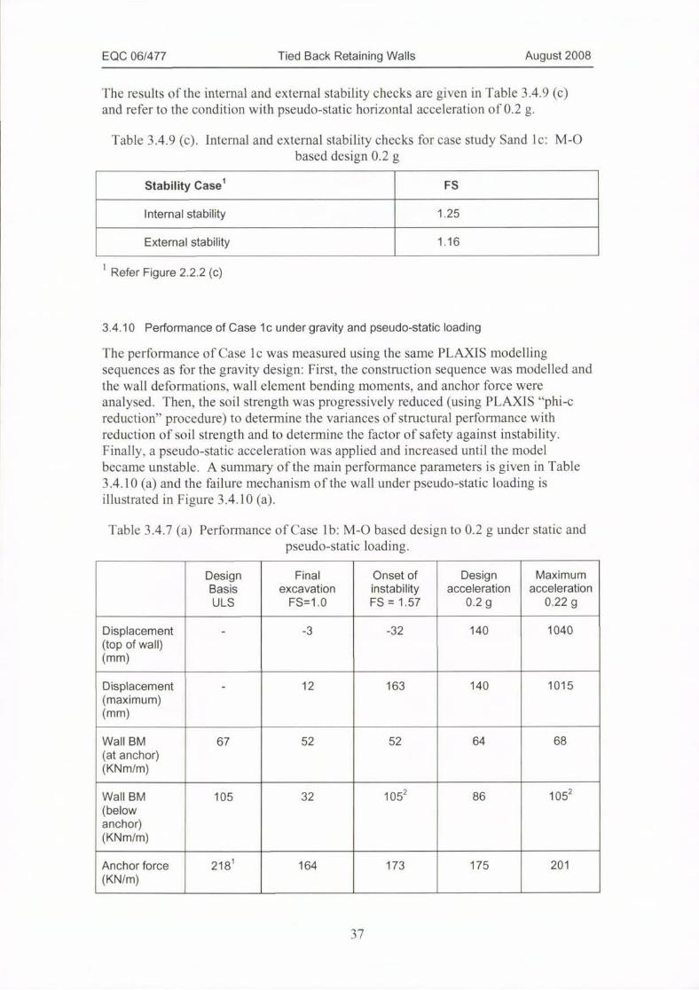
3.4.10 Performance of Case lc under gravity and pseudo-static loading
The performance of Case 1 c was measured using the same PLAXIS modellingsequences as for the gravity design: First, the construction sequence was modelled andthe wall deformations, wall element bending moments, and anchor force wereanalysed. Then, the soil strength was progressively reduced (using PLAXIS "phi-creduction" procedure) to determine the variances of structural performance withreduction of soil strength and to determine the factor of safety against instability.Finally, a pseudo-static acceleration was applied and increased until the modelbecame unstable. A summary ofthe main performance parameters is given in Table3.4.10 (a) and the failure mechanism of the wall under pseudo-static loading isillustrated in Figure 3.4.10 (a).
Table 3.4.7 (a) Performance of Case lb: M-O based design to 0.2 g under static andpseudo-static loading.
Design Final Onset of Design Maximum
Basis excavation instability acceleration acceleration
ULS FS=1.0 FS = 1.57 0.2 g 0.22 g
Displacement - -3 -32 140 1040
(top of wall)(mm)
Displacement - 12 163 140 1015
(maximum)(mm)
Wall BM 67 52 52 64 68
(at anchor)(KNm/m)
Wall BM 105 32 105
(belowanchor)(KNm/m)
286 105
2
Anchor force 218
(KN/m)
164 173 175 201
37
EQC 06/477 Tied Back Retaining Walls August 2008
1 ULS capacity of anchor may be assumed to be the anchor test load, normally set at 80percent of tendon characteristic breaking load, so anchor load of 159 KN/m (92 percent ofcharacteristic breaking load) exceeds the test load but anchor is considered unlikely to fail.2 Wall element is yielding in bending.
As for the gravity only design (Case 1 a), the collapse mechanism of the wall undergravity only loading appears to be hinging of the wall element with significant"bulging" of the wall into the excavation and development of an active soil wedgebehind the wall. The strength of the wall element is. therefore, limiting the factor ofsafety. In this case the anchor force hardly increases above its initial pre-load valueand well below the test load.
*1//04, 9/afi
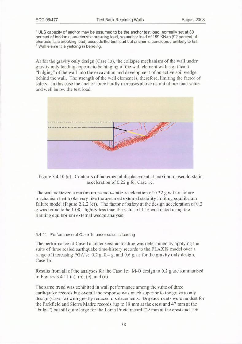
Figure 3.4.10 (a). Contours of incremental displacement at maximum pseudo-staticacceleration of 0.22 g for Case l c.
The wall achieved a maxinium pseudo-static acceleration of 0.22 g with a failure
mechanism that looks very like the assumed external stability limiting equilibriumfailure model (Figure 2.2.2 (c)). The factor of safety at the design acceleration of 0.2g was found to be 1.08, slightly less than the value of 1.16 calculated using thelintiting equilibrium external wedge analysis.
3.4.11 Performance of Case lc under seismic loading
The performance of Case 1 c under seismic loading was determined by applying thesuite of three scaled earthquake time-history records to the PLAXIS model over arange of increasing PGA's: 0.2 g, 0.4 g. and 0.6 g, as for the gravity only design,Case la.
Results from all of the analyses for the Case lc: M-O design to 0.2 g are summarisedin Figures 3.4.11 (a), (b), (c), and (d).
The same trend was exhibited in wall performance among the suite ofthreeearthquake records but overall the response was much superior to the gravity onlydesign (Case la) with greatly reduced displacements: Displacements were modest forthe Parkfield and Sierra Madre records (up to 18 min at the crest and 47 mni at the"bulge") but sill quite large for the Loma Prieta record (29 min at the crest and 106
38
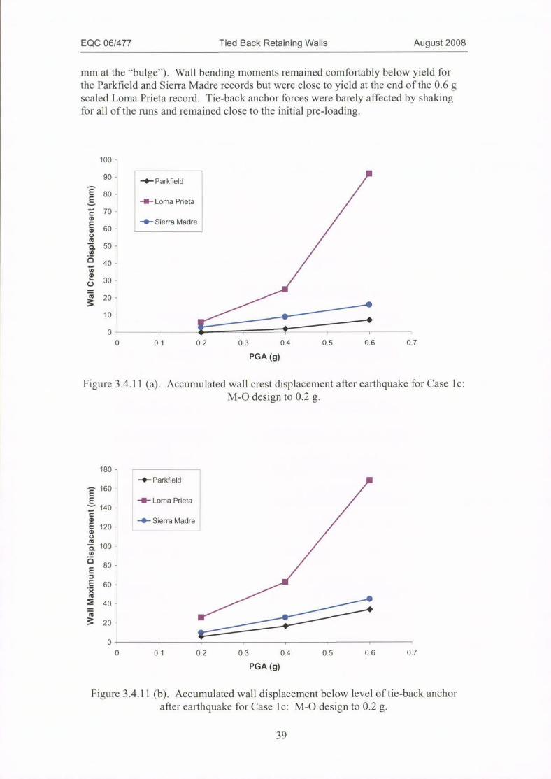
EQC 06/477 Tied Back Retaining Walls August 2008
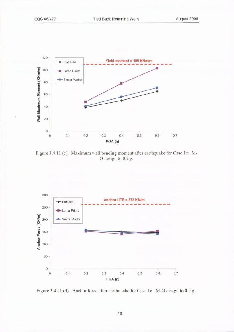
mm at the "bulge"). Wall bending moments remained comfortably below yield forthe Parkfield and Sierra Madre records but were close to yield at the end ofthe 0.6 gscaled Loma Prieta record. Tie-back anchor forces were barely affected by shakingfor all of the runs and remained close to the initial pre-loading.
100 -
90 -+-Parkfield
80 -
-ll- Loma Prieta
70
-·» Sierra Madre60 -
50 -
40 -
30 -
20 -
10 -
0
0 0.1 0.2 0.3 0.4 0.5 0.6 0.7
PGA (g)
Figure 3.4.11 (a). Accumulated wall crest displacement after earthquake for Case 1 c:M-O design to 0.2 g.
180 -
-0- Parkfield JI· 160 -
--- Loma Prieta
0 140 -
-O- Sierra Madre120 -
100
80 -
60 -
40
20 -
0
0 0.1 0.2 0.3 0.4 0.5 0.6 0.7
PGA (g)
Figure 3.4.11 (b). Accumulated wall displacement below level oftie-back anchorafter earthquake for Case le: M-O design to 0.2 g.
39
EQC 06/477 Tied Back Retaining Walls August 2008
120
-+- ParkfieldYield moment = 105 KNrn/m
100 -Il- Loma Prieta /...
+ Sierra Madre
80 X
60
40 -
20 -
0
0 0.1 0.2 0.3 0.4 0.5 0.6 0.7
PGA (g)
Figure 3.4.11 (c). Maximum wall bending moment after earthquake for Case lc: M-O design to 0.2 g.
300 -
Anchor UTS = 272 KN/m+- Parkfield
250 -
-il-Loma Prieta
200 - -O- Sierra Madre
C)
0
8 150 .====e==eMI==-----EE'.L
100 -
50 -
0
0 0.1 0.2 0.3 0.4 0.5 0.6 0.7
PGA (g)
Figure 3.4.11 (d). Anchor force after earthquake for Case le: M-0 design to 0.2 g..
40

EQC 06/477 Tied Back Retaining Walls August 2008
Generally, the performance ofthe wall was good and showed a marked improvementin performance over the gravity only design although at the cost of significantly morematerials in both wall elements and anchors. A more detailed comparison among allthe design cases is given in Section 3.4.18.
3.4.12 Case ld: M-O based design to 0.3 g
The wall for Case 1 d was designed using the synthesized procedure for earthquakedesign outlined in Section 2.3.6. Detailed calculations are given in Appendix A andare summarised here:
Table 3.4.12 (a). Design values for case study Sand ld: M-O based design 0.3 g
Design Parameter Value
Design acceleration 0.3 g
Apparent earth pressure, p 52 KN/m2
Anchor design load (horizontal) 191 KN/m
Base reaction 53 KN/m
Negative bending moment (at anchor) 50 KNm/m
Maximum bending moment (below anchor) 79 KNm/m
ULS design bending moment, M* 126 KNm/m
The wall structural elements were designed using these basic calculated design valuesas follows. For the purposes of this research project, design solutions were perfectlyoptimised, whereas for everyday design it would be necessary to select from standardproducts (e.g. standard anchor configurations, stock steel sections).
Table 3.4.12 (b). Design solutions for case study Sand ld: M-O based design 0.3 g.
Design Solution Value
Anchor cross-section (using super strandanchors at 2 m centres, inclined 15 degrees))
356 mm2 per anchor(3.56 strands per anchor)
Anchor free length 8m
Soldier piles (UC sections set in 450 mm
diameter concrete @2m crs)
95% 1 of 250UC72.9
Depth of embedment 3.3 m
1 Section properties scaled for purpose of the study.
The anchor free length for Case 1 d was determined from the inclination of the M-O
active wedge slip plane calculated for the soil strength reduced by the factor o f safetyfor internal stability. This adjustment has the effect of increasing the free length to
41

EQC 06/477 Tied Back Retaining Walls August 2008
allow for uncertainty in soil strength parameter and ensure that the anchor free lengthextends beyond the active soil zone in all cases.
rhe results of the internal and external stability checks are given in Table 3.4.12 (c)and refer to the condition with pseudo-static horizontal acceleration of 0.3 g.
Table 3.4.12 (c). Internal and external stability checks for case study Sand ld: M-0based design 0.3 g
Stability Casel FS
Internal stability 1.18
External stability 1.12
1 Refer Figure 2.2.2 (c)
3.4.13 Performance of Case ld under gravity and pseudo-static loading
The performance of Case 1 d was measured using the same PLAXIS modellingsequences as for the gravity design: First, the construction sequence was modelled andthe wall deformations, wall element bending moments, and anchor force wereanalysed. Then, the soil strength was progressively reduced (using PLAXIS "phi-creduction" procedure) to determine the variances o f structural performance withreduction of soil strength and to determine the factor of safety against instability.Finally, a pseudo-static acceleration was applied and increased until the modelbecame unstable. A summary of the main performance parameters is given in Table3.4.13 (a) and the failure mechanism of the wall under pseudo-static loading isillustrated in Figure 3.4.13 (a).
Table 3.4.13 (a) Performance of Case ld: M-O based design 0.3 g Linder static andpseudo-static loading.
Design End of Onset Design3 Maximum3
Values Construction Instability, acceleration acceleration
(ULS) FS = 1.68 0.3 g 0.234 g
Displacement - -9 -108 - 181(top of wall)(mm)
Displacement - 8 194 - 232
(maximum)(mm)
Wall BM 50 64 40 - 74
(at anchor)(KNm/m)
Wall BM 79 28 126
(belowanchor)(KNm/m)
93
42
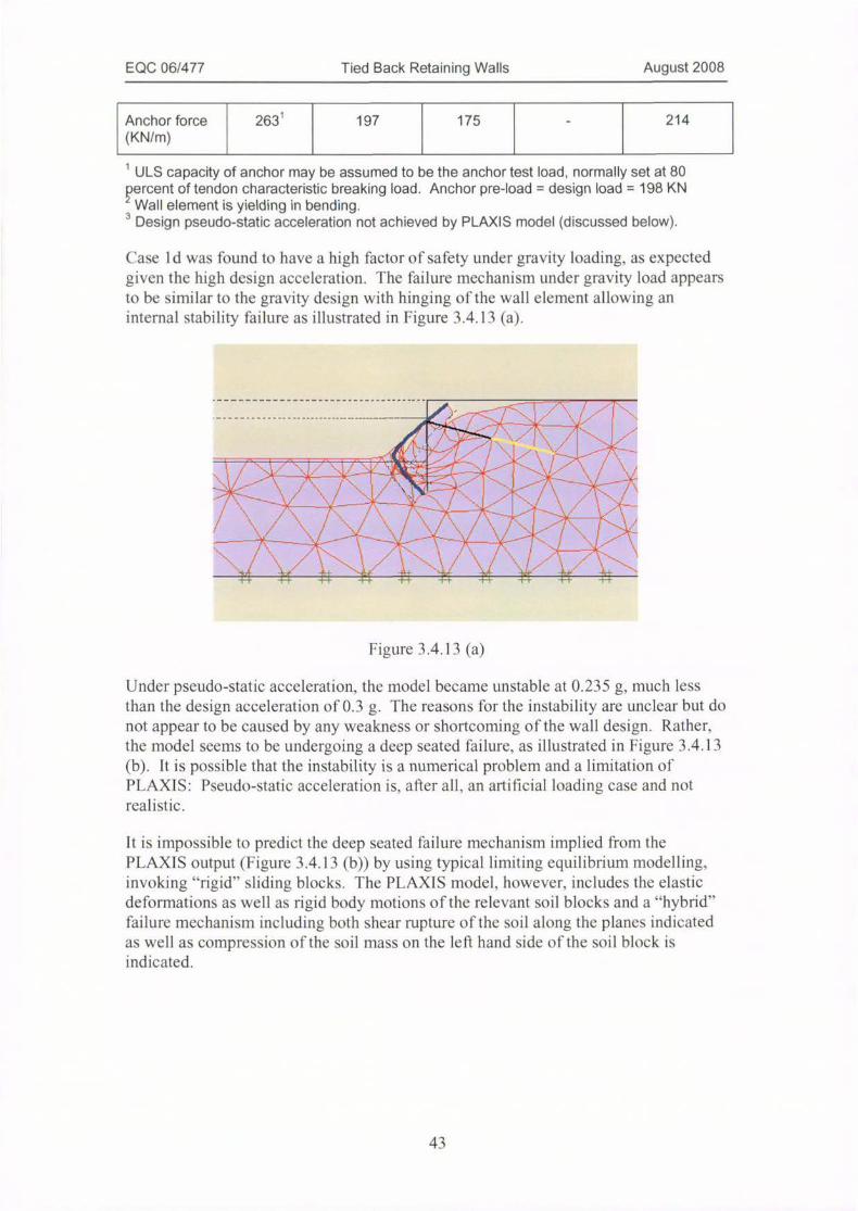
EQC 06/477 Tied Back Retaining Walls August 2008
Anchor force 263
(KN/m)
1197 175 - 214
1 ULS capacity of anchor may be assumed to be the anchor test load, normally set at 80percent of tendon characteristic breaking load. Anchor pre-load = design load = 198 KN
Wall element is yielding in bending.3 Design pseudo-static acceleration not achieved by PLAXIS model (discussed below).
Case 1 d was found to have a high factor o f sa fety under gravity loading, as expectedgiven the high design acceleration. The failure mechanism under gravity load appearsto be similar to the gravity design with hinging of the wall element allowing aninternal stability failure as illustrated in Figure 3.4.13 (a).
9 afl
%31@@.
Figure 3.4.13 (a)
Under pseudo-static acceleration. the model became unstable at 0.235 g, much lessthan the design acceleration of 0.3 g. The reasons for the instability are unclear but donot appear to be caused by any weakness or shortcoming of the wall design. Rather,the model seems to be undergoing a deep seated failure, as illustrated in Figure 3.4.13(b). It is possible that the instability is a numerical problem and a limitation ofPLAXIS: Pseudo-static acceleration is, after all, an artificial loading case and notrealistic.
It is impossible to predict the deep seated failure mechanism implied from thePLAXIS output (Figure 3,4.13 (b)) by using typical limiting equilibrium modelling,invoking "rigid" sliding blocks. The PLAXIS model, however. includes the elasticdeformations as well as rigid body motions ofthe relevant soil blocks and a "hybrid"failure mechanism including both shear rupture of the soil along the planes indicatedas well as compression ofthe soil mass on the left hand side of the soil block isindicated.
43
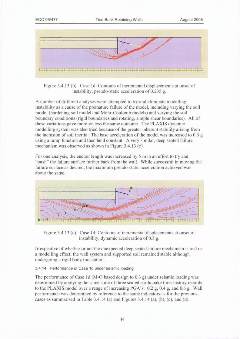
EQC 06/477 Tied Back Retaining Walls August 2008
1/ 11 11 11 11 '' ll li li 11 11 !I ll 'I ll •' •! 1, • •l f' ·J 1111 1111 11 11'1'11 1 11 ·' 11 1. lili ·' 11 Lt14 11 1' LI 1 1 1 11 11 11 li li '1 11 11 , 11 Il 11 11 il 11 1'.
Figure 3.4.13 (b). Case ld: Contours of incremental displacements at onset ofinstability, pseudo-static acceleration ofO.235 g.
A number of different analyses were attempted to try and eliminate modelling
instability as a cause of the premature failure of the model, including varying the soil
model (hardening soil model and Mohr-Coulomb models) and varying the soilboundary conditions (rigid boundaries and rotating, simple shear boundaries). All ofthese variations gave more-or-less the same outcome. The PLAXIS dynamic
modelling system was also tried because of the greater inherent stability arising fromthe inclusion ofsoil inertia: The base acceleration of the model was increased to 0.3 g
using a ramp function and then held constant. A very similar, deep seated failure
mechanism was observed as shown in Figure 3.4.13 (c).
For one analysis, the anchor length was increased by 5 m in an effort to try and
"push" the failure surface further back from the wall. While successful in moving the
failure surface as desired, the maximum pseudo-static acceleration achieved wasabout the same.
«1«12214
%---9-3• ' --I./--- VI----M--
F I' l l 1 1--TT-1 f I T·-r-T-1-,Iif,..1-Ll_11.1_Lt 1 I I f' '' '' '' ' ---' -+i'lithii,ii, „tiii,ini iii-tii,i ii„i,ii tiiiiiii 11 1 11111 iii,iiii it '11111 111111 li li 11111111 1111
Figure 3.4.13 (c). Case ld: Contours of incremental displacements at onset ofinstability, dynamic acceleration of 0.3 g.
Irrespective of whether or not the unexpected deep seated failure mechanism is real ora modelling effect, the wall system and supported soil remained stable althoughundergoing a rigid body translation.
3.4.14 Performance of Case ld under seismic loading
I he performance of Case 1 d (M-0 based design to 0.3 g) under seismic loading was
determined by applying the same suite ofthree scaled earthquake time-history recordsto the PLAXIS niodel over a range of increasing PGA's: 0.2 g, 0.4 g, and 0.6 g. Wall
performance was determined by reference to the same indicators as for the previouscases as summarised in Table 3.4.14 (a) and Figures 3.4.14 (a), (b), (c). and (d).
44
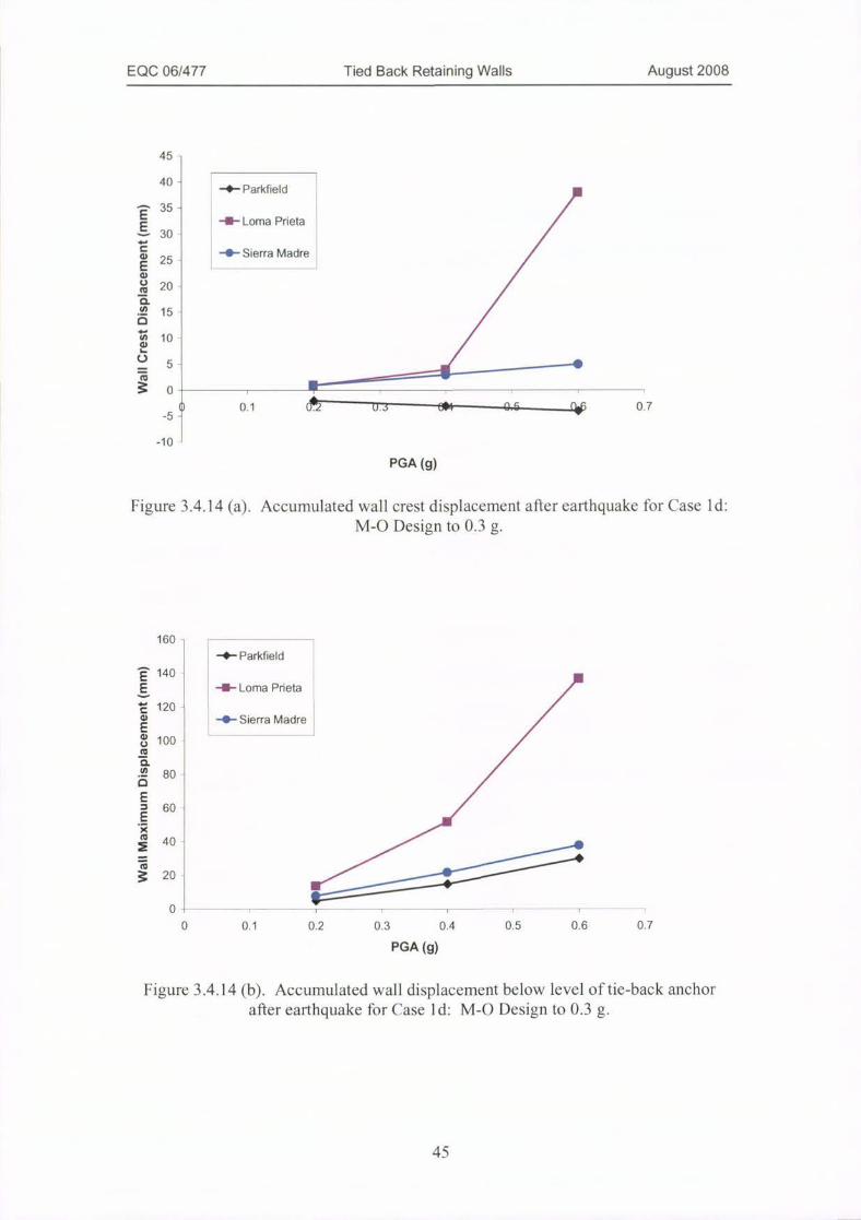
EQC 06/477 Tied Back Retaining Walls August 2008
45 -
40 -
-0- Parkfield /35 -
Al- Loma Prieta
30
-O- Sierra Madre25
20
15
10
5
o
0 0.1 . . 0.7-5 -
-10
PGA (g)
Figure 3.4.14 (a). Accumulated wall crest displacement after earthquake for Case ld:M-O Design to 0.3 g.
160
-0- Parkfield
140
-1# Loma Prieta
120
-O- Sierra Madre
100
80
60
40 -
20
0
0 0.1 0.2 0.3 0.4 0.5 0.6 0.7
PGA (g)
Figure 3.4.14 (b). Accumulated wall displacement below level of tie-back anchorafter earthquake for Case 1 d: M-O Design to 0.3 g.
45
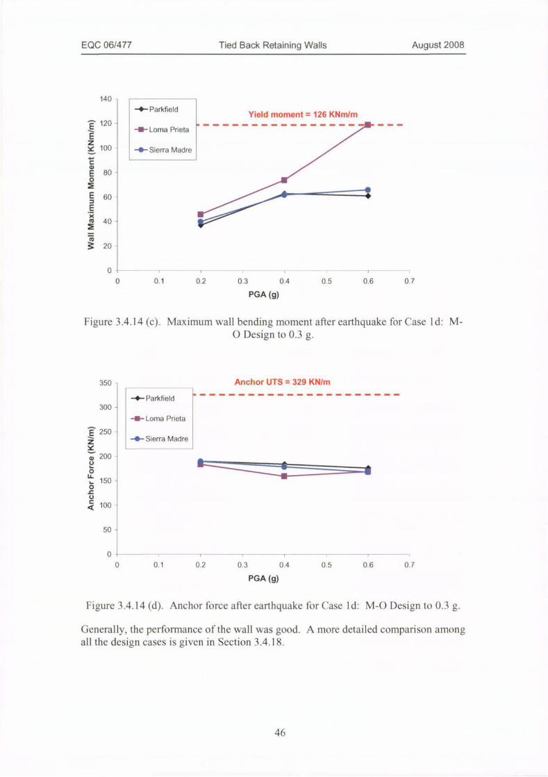
EQC 06/477 Tied Back Retaining Walls August 2008
140 -
-0- ParkfieldYield moment = 126 KNrn/m
120 - ---------
-------- ----ll- Loma Prieta
100 -0- Sierra Madre
80 -
60 -
40- 5
20
0
0 0.1 0.2 0.3 0.4 0.5 0.6 0.7
PGA (g)
Figure 3.4.14 (c). Maximum wall bending moment after earthquake for Case 1 d: M-O Design to 0.3 g.
350 - Anchor UTS = 329 KN/m
-- Parkfield
300 -
--- Lorna Prieta
-O- Sierra Madre
200 -
150 -
kEE.
100
50 -
0
0 0.1 0.2 0.3 0.4 0.5 0.6 0.7
PGA (g)
Figure 3.4.14 (d). Anchor force after earthquake for Case ld: M-O Design to 0.3 g.
Generally, the performance of the wall was good. A more detailed comparison amongall the design cases is given in Section 3.4.18.
46
EQC 06/477 Tied Back Retaining Walls August 2008
3.4.15 Case le: M-O based design to 0.4 g
Ihe wall for Case le was designed using the synthesized procedure for earthquakedesign outlined in Section 2.3.6. Detailed calculations are given in Appendix A andare summarised here:
Table 3.4.15 (a). Design values for case study Sand le: M-O based design 0.4 g
Design Parameter Value
Design acceleration 0.4 g
Apparent earth pressure, p 63.4 KN/m2
Anchor design load (horizontal) 232 KN/m
Base reaction 64 KN/m
Negative bending moment (at anchor) 61 KNm/m
Maximum bending moment (below anchor) 96 KNm/m
ULS design bending moment, M* 153 KNm/m
The wall structural elements were selected using these basic calculated design valuesas follows. For the purposes of this research project, design solutions were perfectlyoptimised, whereas for everyday design it would be necessary to select from standardproducts (e.g. standard anchor configurations, stock steel sections).
I able 3.4.15 (b). Design solutions for case study Sand le: M-0 based design 0.4 g.
Design Solution Value
Anchor cross-section (using super strandanchors at 2 m centres, inclined 15 degrees))
430 mm2 per anchor(4.3 strands per anchor)
Anchor free length 9.2 m
Soldier piles (UC sections set in 450 mm 99%
diameter concrete @2m crs)
of 250UC89.5
Depth of embedment 4.3 m
1 Section properties scaled for purpose of the study.
For Case le the depth of embedment calculated using Broms method (3.8 m) had tobe increased to 4.3 m to provide the desired minimuni factor of safety against internalstability (FS = 1.1 ).
The anchor free length for Case le then was determined from the inclination of the M-O active wedge slip plane calculated for the soil strength reduced by the factor ofsafety for internal stability. This adjustment has the effect of increasing the freelength to allow for uncertainty in soil strength parameter and ensure that the anchorfree length extends beyond the active soil zone in all cases.
47

EQC 06/477 Tied Back Retaining Walls August 2008
The results of the internal and external stability checks are given in Table 3.4.15 (c)and refer to the condition with pseudo-static horizontal acceleration of 0.4 g.
Table 3.4.15 (c). Internal and external stability checks for case study Sand le: M-0based design 0.4 g
Stability Casel FS
Internal stability 1.1
External stability 1.0
1 Refer Figure 2.2.2 (c)
A factor o f safety of 1.0 for external stability is considered to be adequate for thepseudo-static design case. The external stability failure mechanism is considered tobe the preferred mode of yielding for the wall since it is ductile and providesprotection against overloading of the wall elements.
3.4.16 Performance of Case le under gravity and pseudo-static loading
The performance of Case le was measured using the same PLAXIS modellingsequences as for the gravity design: First, the construction sequence was modelled andthe wall deformations, wall element bending moments, and anchor force wereanalysed. Then, the soil strength was progressively reduced (using PLAXIS "phi-creduction" procedure) to determine the variances of structural performance withreduction of soil strength and to determine the factor of safety against instability.Finally, a pseudo-static acceleration was applied and increased until the modelbecame unstable. A summary of the main performance parameters is given in Table3.4.16 (a).
48
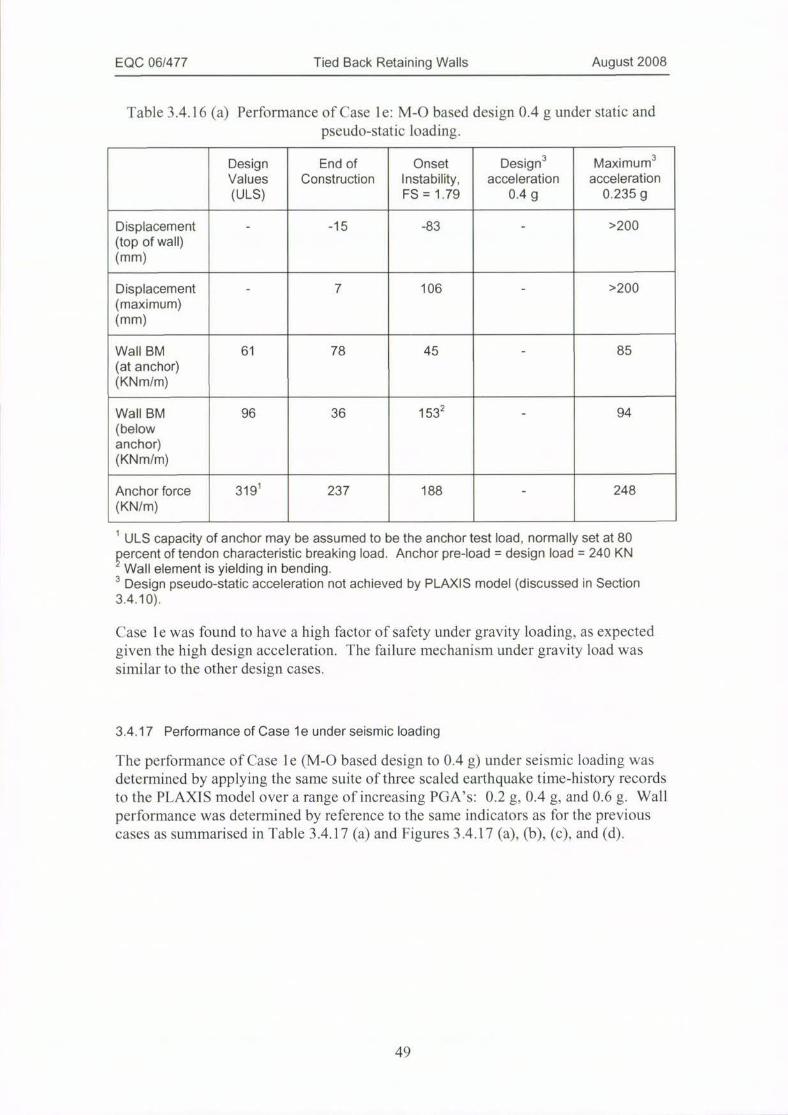
EQC 06/477 Tied Back Retaining Walls August 2008
Table 3.4.16 (a) Performance of Case l e: M-O based design 0.4 g under static andpseudo-static loading.
Design End of Onset Design3 MaximumaValues Construction Instability, acceleration acceleration
(ULS) FS = 1.79 0.4 g 0.235 g
Displacement - -15 -83 - >200
(top of wall)(mm)
Displacement - 7 106 - >200(maximum)(mm)
Wall BM 61 78 45 - 85
(at anchor)(KNm/m)
Wall BM 96 36 153
(belowanchor)(KNm/m)
94
Anchor force 319
(KN/m)
1237 188 - 248
1 ULS capacity of anchor may be assumed to be the anchor test load, normally set at 80percent of tendon characteristic breaking load. Anchor pre-load = design load = 240 KN
Wall element is yielding in bending.3 Design pseudo-static acceleration not achieved by PLAXIS model (discussed in Section3.4.10).
Case 1 e was found to have a high factor of safety under gravity loading, as expectedgiven the high design acceleration. The failure mechanism under gravity load wassimilar to the other design cases.
3.4.17 Performance of Case le under seismic loading
The performance of Case le (M-O based design to 0.4 g) Linder seismic loading wasdetermined by applying the same suite of three scaled earthquake time-history recordsto the PLAXIS model over a range of increasing PGA's: 0.2 g, 0.4 g, and 0.6 g. Wallperformance was determined by reference to the same indicators as for the previouscases as summarised in Table 3.4.17 (a) and Figures 3.4.17 (a), (b), (c), and (d).
49
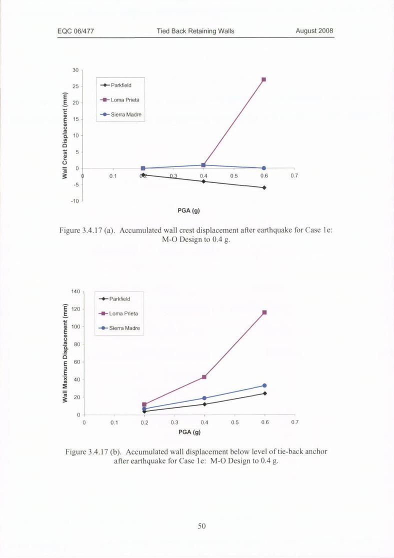
EQC 06/477 Tied Back Retaining Walls August 2008
30
25 +- Parkfield
--- Loma Prieta20
-O- Sierra Madre15 -
10 -
5
O
0 0.1 . 0.4 0.5 0.6 0.7
-5
-10
PGA (g)
Figure 3.4.17 (a). Accumulated wall crest displacement after earthquake for Case 1 e:M-O Design to 0.4 g.
140
-0- Parkfield
-4F Loma Prieta
100 - -O- Sierra Made
80
60 -
40
20 Glzm:0
0 0.1 0.2 0.3 0.4 0.5 0.6 0.7
PGA (g)
Figure 3.4.17 (b). Accumulated wall displacement below level of tie-back anchorafter earthquake for Case le: M-O Design to 0.4 g.
50

EQC 06/477 Tied Back Retaining Walls August 2008
Yield moment = 153 KNm/m150 -
------------------
-+- Parkfield
130
-I- Lorna Prieta
110
-- Sierra Madre
90 -
50 - F-$30
10
-10 0 0.1 0.2 0.3 0.4 0.5 0.6 0.7
PGA (g)
Figure 3.4.17 (c). Maximum wall bending moment after earthquake for Case le: M-O Design to 0.4 g.
Anchor UTS = 397 KN/m
400 -
+- Parkfield350 -
--- Loma Prieta
. 300
-O- Sierra Madre
250 -
D
5 200L
150
100
50
0
0 0.1 0.2 0.3 0.4 0.5 0.6 0.7
PGA (g)
Figure 3.4.17 (d). Anchor force after earthquake for Case le: M-O Design to 0.4 g.
51
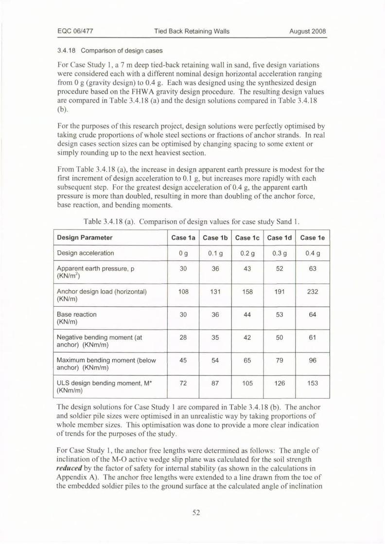
EQC 06/477 Tied Back Retaining Walls August 2008
3.4.18 Comparison of design cases
For Case Study l,a7m deep tied-back retaining wall in sand, five design variationswere considered each with a different nominal design horizontal acceleration rangingfrom 0 g (gravity design) to 0.4 g. Each was designed using the synthesized designprocedure based on the FHWA gravity design procedure. The resulting design valuesare compared in Table 3.4.18 (a) and the design solutions compared in Table 3.4.18(b).
For the purposes of this research project, design solutions were perfectly optimised bytaking crude proportions of whole steel sections or fractions of anchor strands. In realdesign cases section sizes can be optimised by changing spacing to some extent orsimply rounding up to the next heaviest section.
From Table 3.4.18 (a), the increase in design apparent earth pressure is modest for thefirst increment of design acceleration to 0.1 g, but increases more rapidly with eachsubsequent step. For the greatest design acceleration of 0,4 g, the apparent earthpressure is more than doubled, resulting in more than doubling ofthe anchor force,base reaction, and bending moments.
Table 3.4.18 (a). Comparison of design values fur case study Sand 1.
Design Parameter Case la Case lb Case lc Case ld Case le
Design acceleration 0 g 0.1 g 0.2 g 0.3 g 0.4 g
Apparent earth pressure, p 30 36 43 52 63(KN/m2)
Anchor design load (horizontal) 108 131 158 191 232
(KN/m)
Base reaction 30 36 44 53 64
(KN/m)
Negative bending moment (at 28 35 42 50 61anchor) (KNm/m)
Maximum bending moment (below 45 54 65 79 96anchor) (KNm/m)
ULS design bending moment, M* 72 87 105 126 153
(KNm/m)
The design solutions for Case Study 1 are compared in Table 3.4.18 (b). The anchorand soldier pile sizes were optimised in an unrealistic way by taking proportions ofwhole member sizes. This optimisation was done to provide a more clear indicationof trends for the purposes of the study.
For Case Study 1, the anchor free lengths were determined as follows: The angle ofinclination of the M-0 active wedge slip plane was calculated for the soil strengthreduced by the factor of safety for internal stability (as shown in the calculations inAppendix A). The anchor free lengths were extended to a line drawn from the toe ofthe embedded soldier piles to the ground surface at the calculated angle of inclination
52
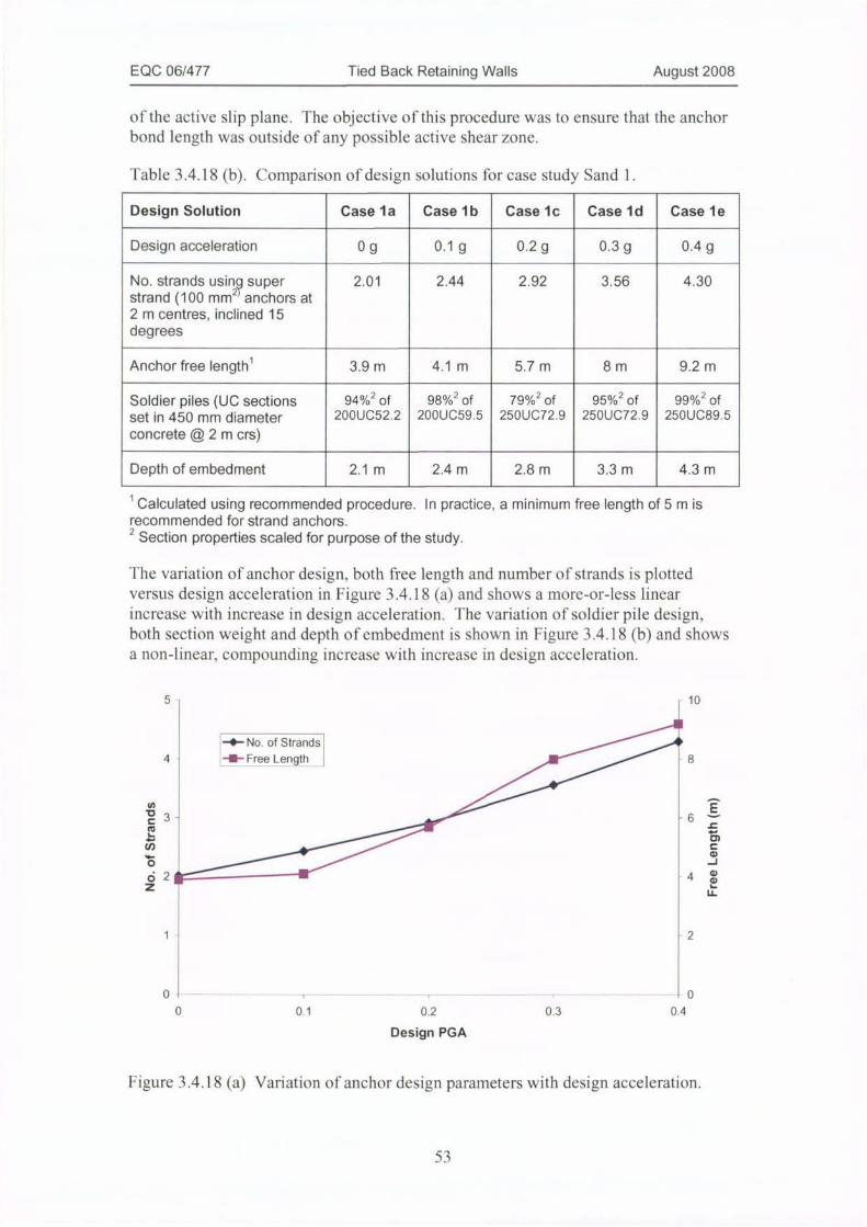
EQC 06/477 Tied Back Retaining Walls August 2008
ofthe active slip plane. The objective of this procedure was to ensure that the anchorbond length was outside of any possible active shear zone.
Table 3.4.18 (b). Comparison of design solutions for case study Sand 1.
Design Solution Case la Case lb Case lc Case 1 d
Design acceleration 0 g 0.1 g 0.2g 0.3 g
No. strands usin super 2.01 2.44 2.92 3.56
strand (100 mm2 anchors at2 m centres, inclined 15degrees
Case 1 e
0.4 g
4.30
Anchor free lengthl 3.9 m 4.1 m 5.7 m 8m 9.2 m
Soldier piles (UC sections 94%2 of 98%2 of 79%2 of 95%2 of 99%2 of
set in 450 mm diameter 200UC52.2 200UC59.5 250UC72.9 250UC72.9 250UC89.5
concrete @2m crs)
Depth of embedment 2.1 m 2.4 m 2.8 m 3.3 m 4.3 m
1 Calculated using recommended procedure. In practice, a minimum free length of 5 m isrecommended for strand anchors.
2 Section properties scaled for purpose of the study.
The variation of anchor design, both free length and number of strands is plottedversus design acceleration in Figure 3.4.18 (a) and shows a more-or-less linearincrease with increase in design acceleration. The variation of soldier pile design,both section weight and depth ofembedment is shown in Figure 3.4.18 (b) and showsa non-linear, compounding increase with increase in design acceleration.
5 10
!+ No. of Strands
4 -I- Free Length 8
M E
C J- -6 -
2 1
4
1 2
0 , , 0
0 0.1 0.2 0.3 0.4
Design PGA
Figure 3.4.18 (a) Variation of anchor design parameters with design acceleration.
53
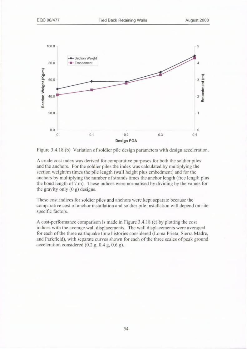
EQC 06/477 Tied Back Retaining Walls August 2008
100.0 - F 5
-0- Section Weight80.0 - -- Embedment /37 -4
60.0 - -3
40.0 - -2
20.0 - -1
0.0 i , , 0
0 0.1 0.2 0.3 0.4
Design PGA
Figure 3.4.18 (b) Variation of soldier pile design parameters with design acceleration.
A crude cost index was derived fur comparative purposes for both the soldier pilesand the anchors. For the soldier piles the index was calculated by multiplying thesection weight/m times the pile length (wall height plus embedment) and for theanchors by multiplying the number of strands times the anchor length (free length plus
the bond length of 7 m). These indices were normalised by dividing by the values forthe gravity only (0 g) designs.
These cost indices for soldier piles and anchors were kept separate because thecomparative cost of anchor installation and soldier pile installation will depend on sitespecific factors.
A cost-performance comparison is made in Figure 3.4.18 (c) by plotting the costindices with the average wall displacements. The wall displacements were averagedfor each of the three earthquake time histories considered (Loma Prieta, Sierra Madre,and Parkfield), with separate curves shown for each of the three scales of peak groundacceleration considered (0.2 g, 0.4 g, 0.6 g)..
54
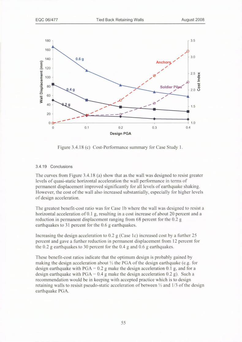
EQC 06/477 Tied Back Retaining Walls August 2008
180 - F 3.5
L
160 -
140 - \2.6 g.120
100 -
80 0\11:4 g
60 -
40 220 - --
0
e
Anchor;
Soldier Pilps"
-- - - Illy
3.0
2.5 ZC
0
2.0 0
15
, , 1.0
0 0.1 0.2 0.3 0.4
Design PGA
Figure 3.4.18 (c) Cost-Performance summary for Case Study 1.
3.4.19 Conclusions
lee curves from Figure 3.4.18 (a) show that as the wall was designed to resist greaterlevels of quasi-static horizontal acceleration the wall performance in terms ofpermanent displacement improved significantly for all levels of earthquake shaking.Ilowever, the cost ofthe wall also increased substantially, especially for higher levelsofdesign acceleration.
Tile greatest benefit-cost ratio was for Case 1 b where the wall was designed to resist ahorizontal acceleration of 0.1 g, resulting in a cost increase ofabout 20 percent and areduction in permanent displacement ranging from 68 percent for the 0.2 gearthquakes to 31 percent for the ().6 g earthquakes.
Increasing the design acceleration to 0.2 g (Case 1 c) increased cost by a further 25percent and gave a further reduction in permanent displacement from 12 percent forthe 0.2 g earthquakes to 30 percent for the 0.4 g and 0.6 g earthquakes.
These benefit-cost ratios indicate that the optimum design is probably gained bymaking the design acceleration about 'h the PGA of the design earthquake (e.g. fordesign earthquake with PGA = 0.2 g make the design acceleration 0.1 g, and for adesign earthquake with PGA = 0.4 g make the design acceleration 0.2 g). Such arecommendation would be in keeping with accepted practice which is to designretaining walls to resisit pseudo-static acceleration of between M and 1/3 ofthe designearthquake PGA.
55
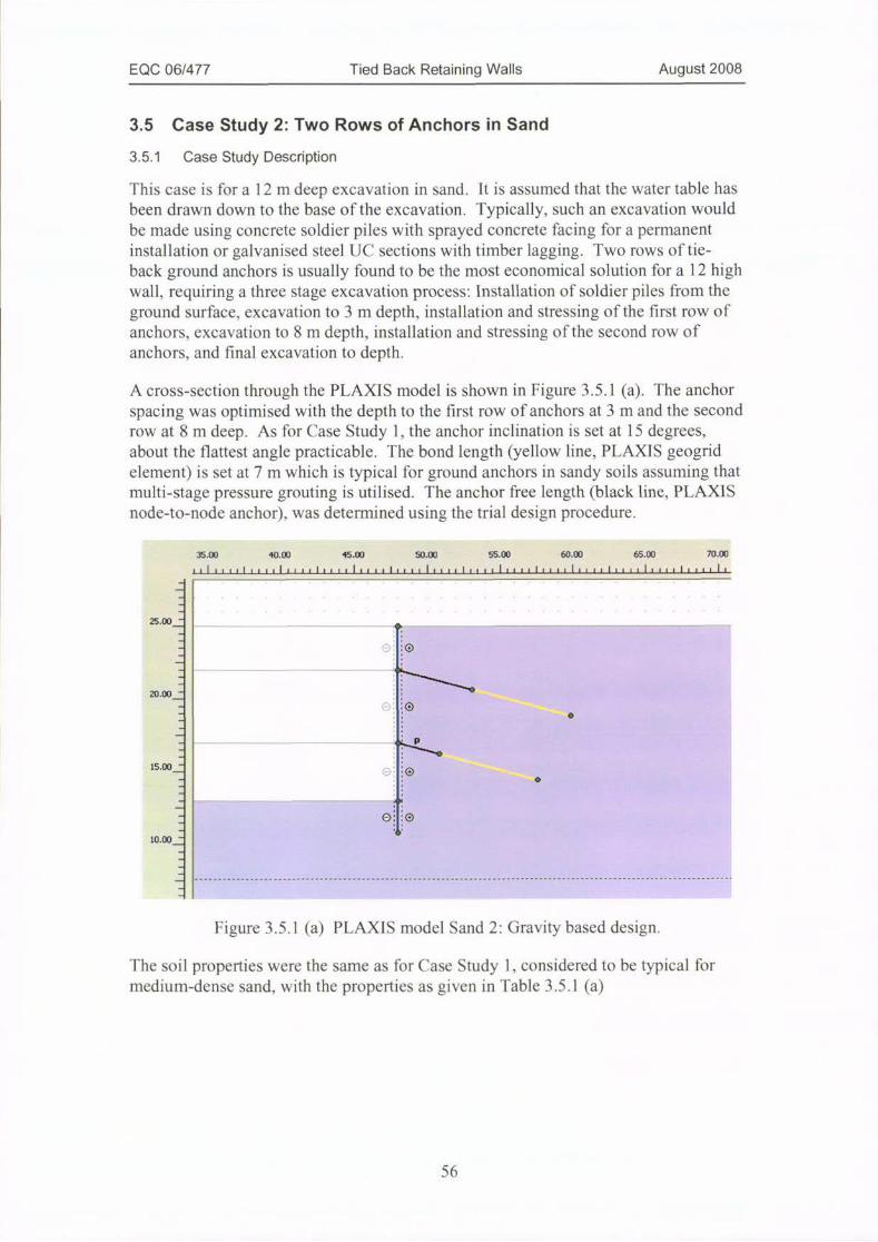
EQC 06/477 Tied Back Retaining Walls August 2008
3.5 Case Study 2: Two Rows of Anchors in Sand
3.5.1 Case Study Description
This case is for a 12 m deep excavation in sand. It is assumed that the water table hasbeen drawn down to the base ofthe excavation. Typically, such an excavation wouldbe made using concrete soldier piles with sprayed concrete facing for a permanentinstallation or galvanised steel UC sections with timber lagging. Two rows of tie-back ground anchors is usually found to be the most economical solution for a12 highwall, requiring a three stage excavation process: 1nstallation of soldier piles from theground surface, excavation to 3 m depth, installation and stressing of the first row ofanchors, excavation to 8 m depth, installation and stressing ofthe second row ofanchors, and final excavation to depth.
A cross-section through the PLAXIS model is shown in Figure 3.5.1 (a). The anchorspacing was optimised with the depth to the first row of anchors at 3 m and the secondrow at 8 m deep. As for Case Study 1, the anchor inclination is set at 15 degrees,about the flattest angle practicable. The bond length (yellow line, PLAXIS geogridelement) is set at 7 m which is typical for ground anchors in sandy soils assuming thatmulti-stage pressure grouting is utilised. The anchor free length (black line, PLAXISnode-to-node anchor), was determined using the trial design procedure.
.//IN.
40.00 45.00 50.00 55.00 60.00 65.00
/iIi/,iI/,,,Itit1I/'i,I,,',Iiii,IiiiiIii,i|I1/1I1i11|1i1llIIi1|l lilli
25.00.
15.00_
10.00_
0 :012£
20.00_
70.00
1 11
Figure 3.5.1 (a) PLAXIS model Sand 2: Gravity based design.
The soil properties were the same as for Case Study 1, considered to be typical formedium-dense sand, with the properties as given in Table 3.5.1 (a)
56
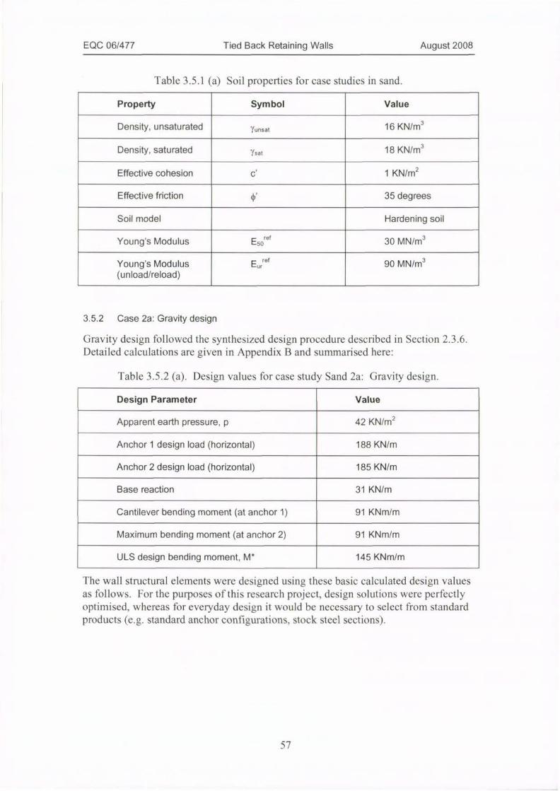
EQC 06/477 Tied Back Retaining Walls August 2008
Table 3.5.1 (a) Soil properties for case studies in sand.
Property Symbol Value
Density, unsaturated Yunsat16 KN/m3
Density, saturated 7sat18 KN/m3
Effective cohesion c' 1 KN/m2
Effective friction ¢' 35 degrees
Soil model Hardening soil
Young's Modulus E5ref 30 MN/%3
ref
Young's Modulus Eur(unload/reload)
90 MN/m3
3.5.2 Case 2a: Gravity design
Gravity design followed the synthesized design procedure described in Section 2.3.6.
Detailed calculations are given in Appendix B and summarised here:
Table 3.5.2 (a). Design values for case study Sand 2a: Gravity design.
Design Parameter Value
Apparent earth pressure, p 42 KN/m2
Anchor 1 design load (horizontal) 188 KN/m
Anchor 2 design load (horizontal) 185 KN/m
Base reaction 31 KN/m
Cantilever bending moment (at anchor 1) 91 KNm/m
Maximum bending moment (at anchor 2) 91 KNm/m
ULS design bending moment, M* 145 KNm/m
The wall structural elements were designed using these basic calculated design valuesas follows. For the purposes of this research project, design solutions were perfectlyoptimised. whereas for everyday design it would be necessary to select from standardproducts (e.g. standard anchor configurations, stock steel sections).
57
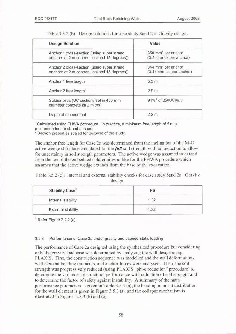
EQC 06/477 Tied Back Retaining Walls August 2008
Table 3.5.2 (b). Design solutions for case study Sand 2a: Gravity design.
Design Solution Value
Anchor 1 cross-section (using super strandanchors at 2 m centres, inclined 15 degrees))
350 mm2 per anchor(3.5 strands per anchor)
Anchor 2 cross-section (using super strandanchors at 2 m centres, inclined 15 degrees))
344 mm2 per anchor(3.44 strands per anchor)
Anchor 1 free length 5.3 m
Anchor 2 free lengthl 2.9 m
Soldier piles (UC sections set in 450 mm 94%
diameter concrete @2m crs)
2 of 250UC89.5
Depth of embedment 2.2 m
1 Calculated using FHWA procedure. In practice, a minimum free length of 5 m isrecommended for strand anchors.
2 Section properties scaled for purpose of the study.
[he anchor free length for Case 2a was determined from the inclination of the M-0active wedge slip plane calculated for the full soil strength with no reduction to allowfor uncertainty in soil strength parameters. The active wedge was assumed to extendfrom the toe of the embedded soldier piles unlike for the FHWA procedure whichassumes that the active wedge extends from the base o f the excavation.
Table 3.5.2 (c). Internal and external stability checks for case study Sand 2a: Gravitydesign.
Stability Casel FS
Internal stability 1.32
External stability 1.32
1 Refer Figure 2.2.2 (c)
3.5.3 Performance of Case 2a under gravity and pseudo-static loading
The performance of Case 2a designed using the synthesized procedure but consideringonly the gravity load case was determined by analysing the wall design usingPLAXIS. First, the construction sequence was modelled and the wall deformations,wall element bending moments, and anchor forces were analysed. Then, the soilstrength was progressively reduced (using PLAXIS "phi-c reduction" procedure) todetermine the variances of structural performance with reduction of soil strength andto determine the factor of safety against instability. A summary of the mainperformance parameters is given in Table 3.5.3 (a), the bending moment distributionfor the wall element is given in Figure 3.5.3 (a), and the collapse mechanism isillustrated in Figures 3.5.3 (b) and (c).
58
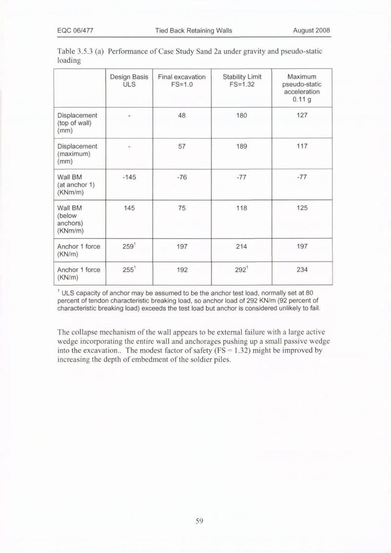
EQC 06/477 Tied Back Retaining Walls August 2008
Table 3.5.3 (a) Performance of Case Study Sand 2a under gravity and pseudo-staticloading
Design Basis Final excavation Stability Limit Maximum
ULS FS=1.0 FS=1.32 pseudo-staticacceleration
0.11 g
Displacement - 48 180 127
(top of wall)(mm)
Displacement - 57 189 117
(maximum)(mm)
Wall BM -145 -76 -77 -77
(at anchor 1)(KNm/m)
Wall BM 145 75 118 125
(belowanchors)(KNm/m)
Anchor 1 force 259
(KN/m)
197 214 197
Anchor 1 force 255
(KN/m)
1192 292 234
1 ULS capacity of anchor may be assumed to be the anchor test load, normally set at 80percent of tendon characteristic breaking load, so anchor load of 292 KN/m (92 percent ofcharacteristic breaking load) exceeds the test load but anchor is considered unlikely to fail.
The collapse mechanism of the wall appears to be external failure with a large activewedge incorporating the entire wall and anchorages pushing up a small passive wedgeinto the excavation.. The modest factor of safety (FS = 1.32) might be improved byincreasing the depth ofembedment of the soldier piles.
59
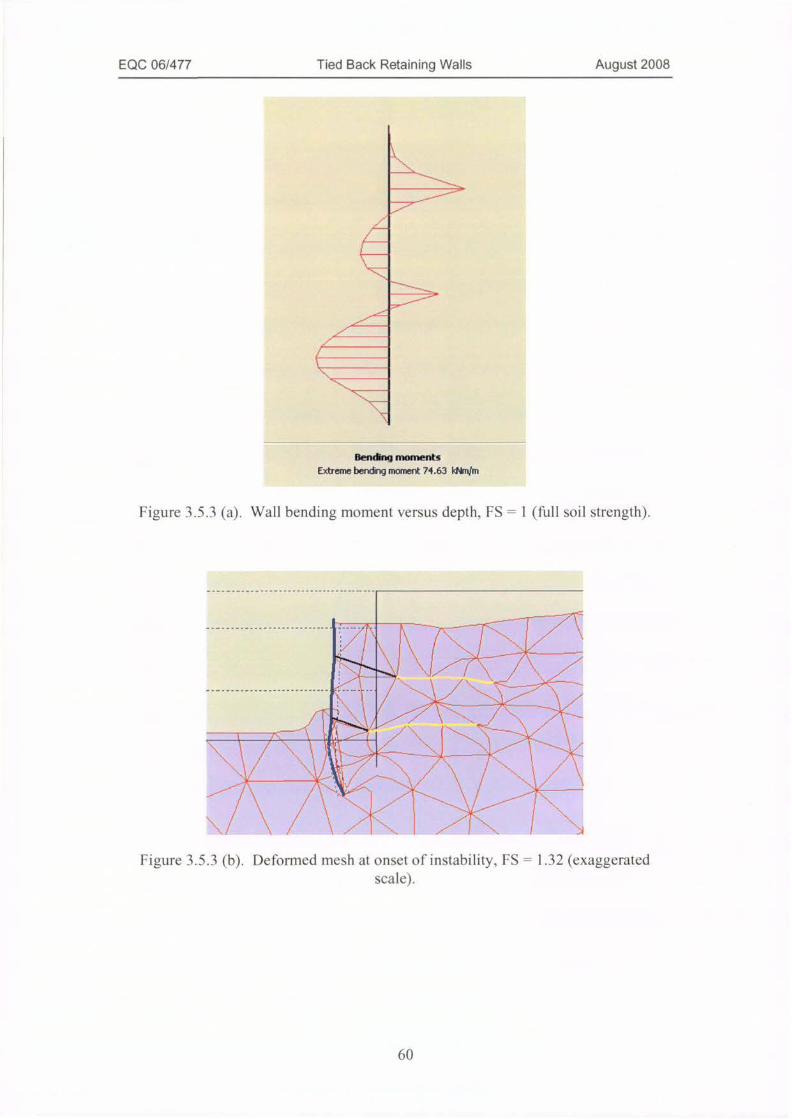
EQC 06/477 Tied Back Retaining Walls August 2008
4
-37
f
1Bencing moments
Extreme bending moment 74.63 INm/m
Figure 3.5.3 (a). Wall bending moment versus depth, FS = 1 (full soil strength).
A
Figure 3.5.3 (b). Deformed mesh at onset o f instability, FS = 1.32 (exaggeratedscale).
60
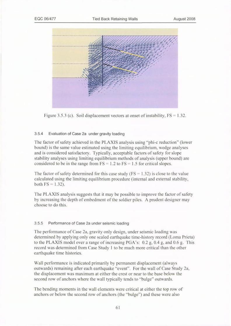
EQC 06/477 Tied Back Retaining Walls August 2008
--7,:5,74,.*4#WA,34,9, :,1"Cilejaiti!,d,mj.M!&1rb./4:i+<-
iq--AW -*7*Ldeit'*M¥1'....
e*spee- /31*42
Figure 3.5.3 (c). Soil displacement vectors at onset of instability, FS = 1.32.
3.5.4 Evaluation of Case 2a under gravity loading
The factor of safety achieved in the PLAXIS analysis using "phi-c reduction" (lowerbound) is the same value estimated using the limiting equilibrium, wedge analysesand is considered satisfactory. Typically, acceptable factors of safety for slopestability analyses using limiting equilibrium methods of analysis (upper bound) areconsidered to be in the range from FS = 1,2 to FS = 1.5 for critical slopes.
The factor of safety determined for this case Stlldy (FS = 1.32) is close to the valuecalculated using the limiting equilibrium procedure (internal and external stability,both FS = 1.32).
The PLAXIS analysis suggests that it may be possible to improve the factor of safetyby increasing the depth of embedment of the soldier piles. A prudent designer maychoose to do this.
3.5.5 Performance of Case 2a under seismic loading
The performance of Case 28, gravity only design, under seismic loading wasdetermined by applying only one scaled earthquake time-history record (Lorna Prieta)to the PLAXIS model over a range of increasing PGA's: 0.2 g, 0.4 g. and 0.6 g. Thisrecord was determined from Case Study 1 to be much more critical than the otherearthquake time histories.
Wall performance is indicated primarily by permanent displacement (alwaysoutwards) remaining after each earthquake "event". For the wall of Case Study 2a,the displacement was maximum at either the crest or near to the base below thesecond row of anchors where the wall typically tends to "bulge" outwards.
I-he bending moments in the wall elements were critical at either the top row ofanchors or below the second row of anchors (the "bulge") and these were also
61
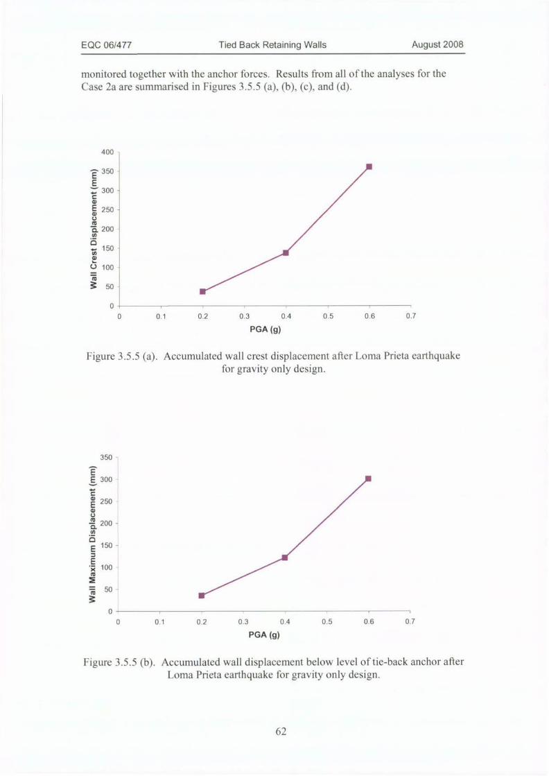
EQC 06/477 Tied Back Retaining Walls August 2008
monitored together with the anchor forces. Results from all of the analyses for theCase 2a are summarised in Figures 3.5.5 (a), (b), (c), and (d).
400
350 -
'300-
150
100
50
0
0 0.1 0.2 0.3 04 0.5 0.6 0.7
PGA (g)
Figure 3.5.5 (a). Accumulated wall crest displacement after Loma Prieta earthquakefor gravity only design.
350 -
,
250
200 -
150 -
100
50 -
0
0 0.1 0.2 0.3 0.4 0.5 0.6 0.7
PGA (g)
Figure 3.5.5 (b). Accumulated wall displacement below level of tie-back anchor afterLoma Prieta earthquake for gravity only design.
62
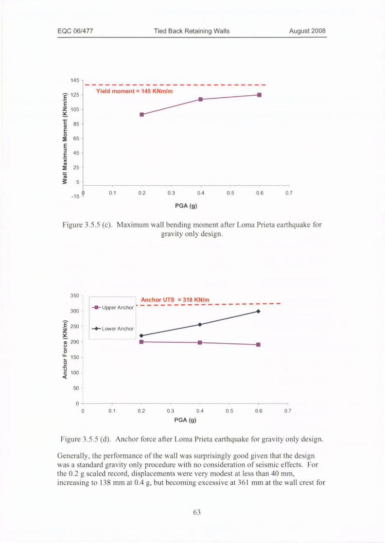
EQC 06/477 Tied Back Retaining Walls August 2008
145-
Yield moment = 145 KNm/m' 125 - -----1
105 -
85 -
65 -
45 -
25
5-
0 0.1 0.2 0.3 0.4 0.5 0.6 0.7-15
PGA (g)
Figure 3.5.5 (c). Maximum wall bending moment after Loma Prieta earthquake forgravity only design.
350 -
300 --- Upper Anchor
Anchor UTS = 318 KN/m
250 --4- Lower Anchor
200 - m .-----------
150 -
100 -
50 -
0
0 0.1 0.2 0.3 0.4 0.5 0.6 0,7
PGA (g)
Figure 3.5.5 (d). Anchor force after Loma Prieta earthquake for gravity only design.
Generally. the performance of the wall was surprisingly good given that the design
was a standard gravity only procedure with no consideration of seismic effects. For
the 0.2 g scaled record, displacements were very modest at less than 40 nim,
increasing to 138 mm at 0.4 g but becoming excessive at 361 mni at the wall crest for
63

EQC 06/477 Tied Back Retaining Walls August 2008
the 0.6 g scaled time history. Wall moment and the lower anchor force were also
increasing to quite high levels by the end ofthe 0.6 g record.
A more detailed comparison among all of the Case 2 design cases is given in Section3.5.12.
3.5.6 Case 2b: M-O based design to 0.1 g
Design of Case 2b followed the synthesized design procedure described in Section2.3.6. Detailed calculations are given in Appendix B and summarised here:
Table 3.5.6 (a). Design values for case study Sand 2b: M-O design to 0.1 g.
Design Parameter Value
Design acceleration 0.1 g
Apparent earth pressure, p 51 KN/m2
Anchor 1 design load (horizontal) 229 KN/m
Anchor 2 design load (horizontal) 224 KN/m
Base reaction 38 KN/m
Cantilever bending moment (at anchor 1) 110 KNm/m
Maximum bending moment (at anchor 2) 110 KNm/m
ULS design bending moment, M* 176 KNm/m
The wall structural elements were designed using these basic calculated design valuesas follows. For the purposes of this research project, design solutions were perfectlyoptimised, whereas for everyday design it would be necessary to select from standard
products (e.g. standard anchor configurations, stock steel sections).
Table 3.5.7 (b). Design solutions for case study Sand 2b: M-O design to 0.1 g.
Design Solution Value
Anchor 1 cross-section (using super strandanchors at 2 m centres, inclined 15 degrees))
426 mm2 per anchor(4.2 strands per anchor)
Anchor 2 cross-section (using super strandanchors at 2 m centres, inclined 15 degrees))
426 mm2 per anchor(4.2 strands per anchor)
Anchor 1 free length 6.3 m
Anchor 2 free lengthl 3.6 m
Soldier piles (UC sections set in 450 mm 83%2 of 310UC96.8
diameter concrete @2m crs)
Depth of embedment 2.5 m
64

EQC 06/477 Tied Back Retaining Walls August 2008
1 Calculated using FHWA procedure. In practice, a minimum free length of 5 m isrecommended for strand anchors.
2 Section properties scaled for purpose of the study.
The anchor free length for Case 2a was determined from the inclination ofthe M-Oactive wedge slip plane calculated for the full soil strength with no reduction to allowfor uncertainty in soil strength parameters. The active wedge was assumed to extendfrom the toe of the embedded soldier piles unlike for the FHWA procedure whichassumes that the active wedge extends from the base of the excavation.
Table 3.5.7 (c). Internal and external stability checks for case study Sand 2b: M-Obased design 0.1 g
1
Stability Casel FS
Internal stability 1.31
External stability 1.13
Refer Figure 2.2.2 (c)
3.5.7 Performance of Case 2b under gravity and pseudo-static loading
The performance of Case 2b was determined using the sanie PLAXIS modellingsequences as for the gravity design: First, the construction sequence was modelled andthe wall deformations, wall element bending moments, and anchor force wereanalysed. Then. the soil strength was progressively reduced (using PLAXIS "phi-creduction" procedure) to determine the variances ofstructural performance withreduction of soil strength and to determine the factor of safety against instability.Finally, a pseudo-static acceleration was applied and increased until the modelbecame unstable. A summary of the main performance parameters is given in Table3.5.7 (a) and the failure mechanism of the wall under pseudo-static loading isillustrated in Figure 3.5.7 (a).
As for the gravity only design (Case 2a). the failure mechanism of the wall under bothgravity only loading and pseudo-static loading appears to be external stability withformation ofa large active wedge of soil encompassing the wall and both anchors, asshown in Figure 3.5.7 (a)
65
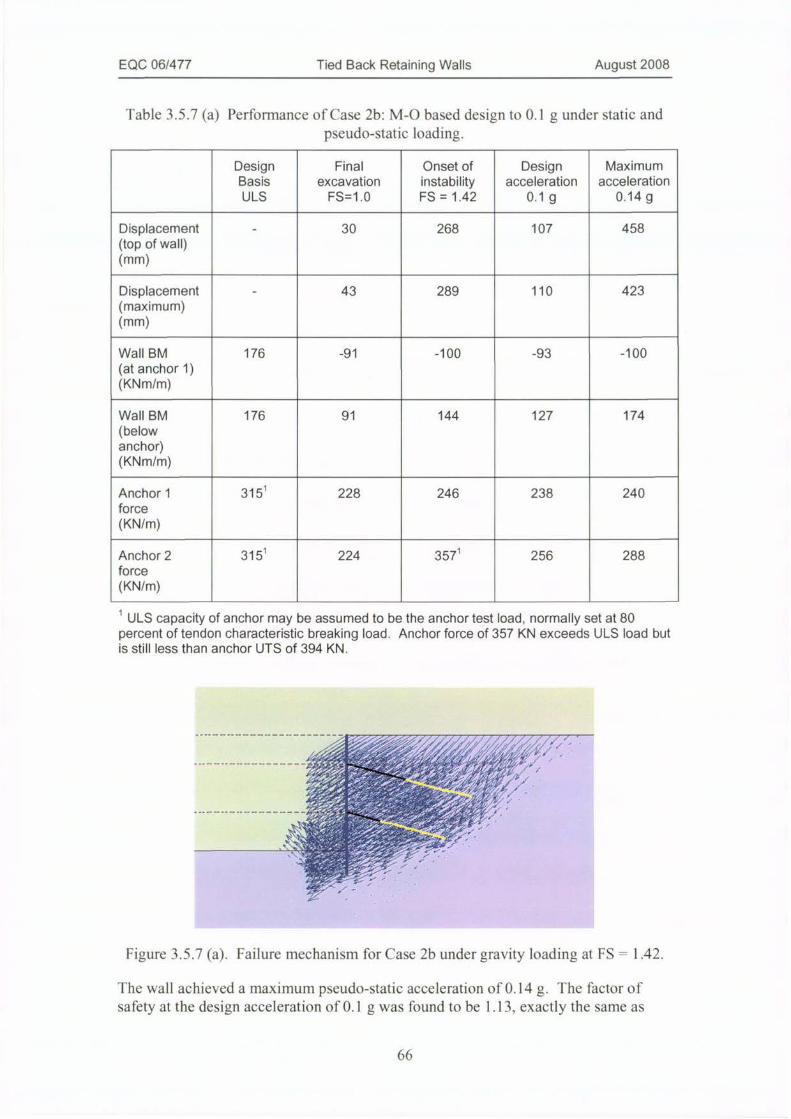
EQC 06/477 Tied Back Retaining Walls August 2008
Table 3.5.7 (a) Performance of Case 2b: M-O based design to 0.1 g under static andpseudo-static loading.
Design Final Onset of Design Maximum
Basis excavation instability acceleration acceleration
ULS FS=1.0 FS = 1.42 0.1 g 0.14 g
Displacement - 30 268 107 458
(top of wall)(mm)
Displacement - 43 289 110 423
(maximum)(mm)
Wall BM 176 -91 -100 -93 -100
(at anchor 1)(KNm/m)
Wall BM 176 91 144 127 174
(belowanchor)(KNm/m)
Anchorl 3151force
(KN/m)
228 246 238 240
Anchor 2 315
force
(KN/m)
1224 3571 256 288
1 ULS capacity of anchor may be assumed to be the anchor test load, normally set at 80percent of tendon characteristic breaking load. Anchor force of 357 KN exceeds ULS load butis still less than anchor UTS of 394 KN.
4'*Af.'Kwaioe,-52227pf2t!E;'18' :-1,
-
30#.5.
Figure 3.5.7 (a). Failure mechanism for Case 2b under gravity loading at FS = 1.42.
1 he wall achieved a maximum pseudo-static acceleration of 0.14 g. The factor of
safety at the design acceleration of 0.1 g was found to be 1.13, exactly the same as
66
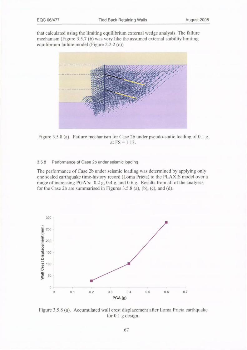
EQC 06/477 Tied Back Retaining Walls August 2008
that calculated using the limiting equilibrium external wedge analysis. The failuremechanism (Figure 3.5.7 (b) was very like the assumed external stability limitingequilibrium failure model (Figure 2.2.2 (c))
,#p-*Urd## AM/'DUL:£ f<AN"di./....../.IA
Figure 3.5.8 (a). Failure mechanism for Case 2b under pseudo-static loading of 0.1 gat FS = 1.13.
3.5.8 Performance of Case 2b under seismic loading
The performance of Case 2b under seismic loading was determined by applying onlyone scaled earthquake time-history record (Loma Prieta) to the PLAXIS model over arange of increasing PGA's: 0.2 g, 0.4 g. and 0.6 g. Results from all ofthe analysesfur the Case 2b are summarised in Figures 3.5.8 (a). (b). (c),and (d).
300
250
200
150
100 ,
50
0
0 01 0.2 0.3 0.4 0.5 0.6 0,7
PGA (g)
Figure 3.5.8 (a). Accumulated wall crest displacement after Lorna Prieta earthquakefor 0.1 g design.
67

EQC 06/477 Tied Back Retaining Walls August 2008
300 -
.250 -
200 -
150 -
50 -
0
0 0.1 0.2 0.3 0.4 0.5 0.6 0.7
PGA (g)
Figure 3.5.8 (b). Accumulated wall displacement below level of tie-back anchor afterLoma Prieta earthquake for 0.1 g design.
200 -
Yield moment = 176 KNrn/m
150 - ,----
100
50 -
0 1 1 1 1 1 1
0 0.1 0.2 0.3 0.4 0.5 0.6 0.7
PGA (g)
Figure 3.5.8 (c). Maximum wall bending moment after Loma Prieta earthquake for0.1 g design.
68
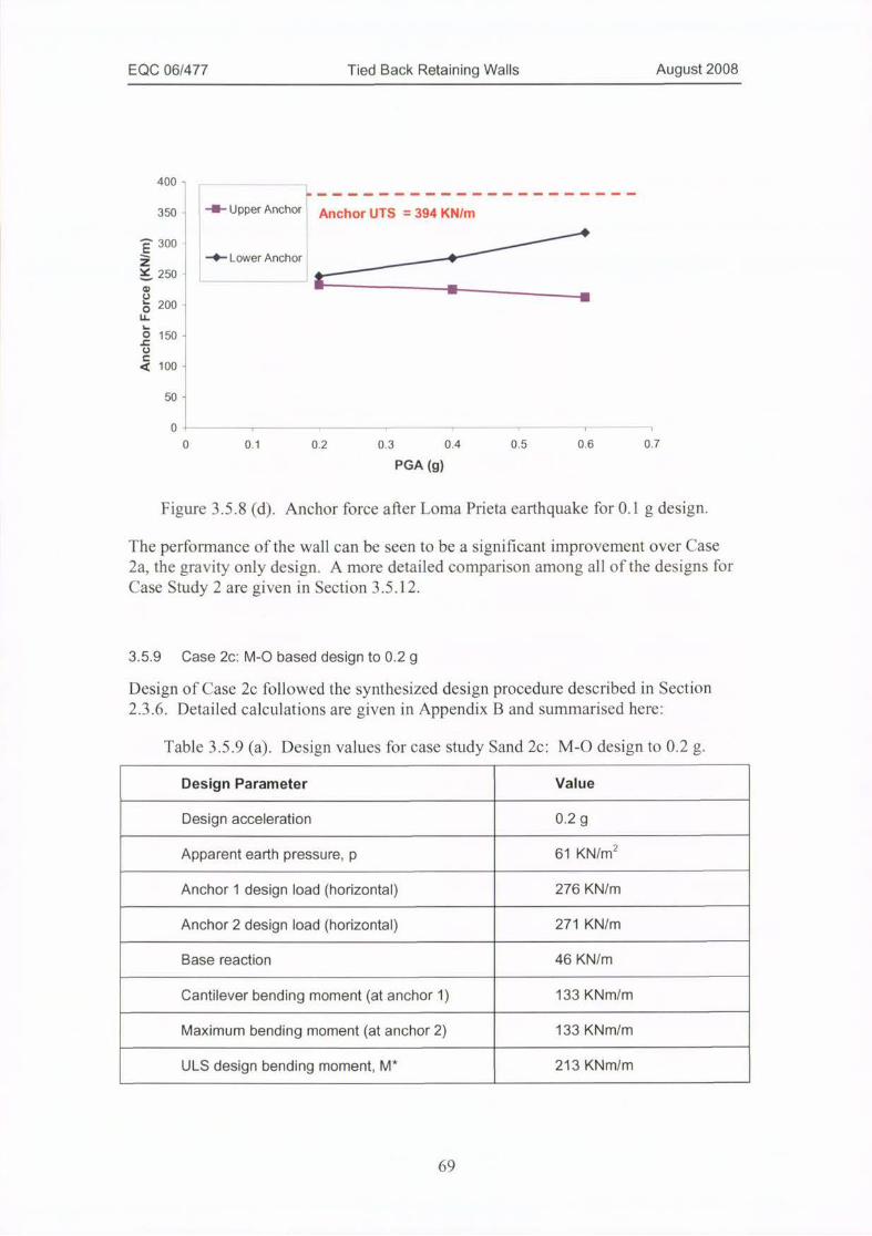
EQC 06/477 Tied Back Retaining Walls August 2008
400 -
350 - -- Upper Anchor Anchor UTS = 394 KN/m
* 300
-0- Lower Anchor --+250-
200 -
150 -
100 -
50 -
0
0 0.1 0.2 0.3 0.4 0.5 0.6 0.7
PGA (g)
Figure 3.5.8 (d). Anchor force after Loma Prieta earthquake for 0.1 g design.
The performance of the wall can be seen to be a significant improvement over Case2a, the gravity only design. A more detailed comparison among all of the designs forCase Study 2 are given in Section 3.5.12.
Case 2c: M-O based design to 0.2 g
Design of Case 2c followed the synthesized design procedure described in Section2.3.6. Detailed calculations are given in Appendix B and summarised here:
Table 3.5.9 (a). Design values for case study Sand 2c: M-0 design to 0.2 g.
Design Parameter Value
Design acceleration 0.2 g
Apparent earth pressure, p 61 KN/m2
Anchor 1 design load (horizontal) 276 KN/m
Anchor 2 design load (horizontal) 271 KN/m
Base reaction 46 KN/m
Cantilever bending moment (at anchor 1) 133 KNm/m
Maximum bending moment (at anchor 2) 133 KNm/m
ULS design bending moment, M* 213 KNm/m
69
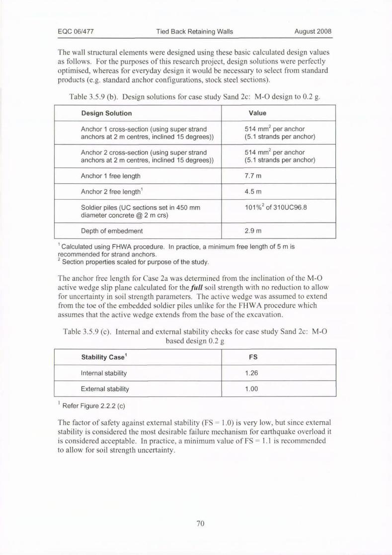
EQC 06/477 Tied Back Retaining Walls August 2008
The wall structural elements were designed using these basic calculated design valuesas follows. For the purposes of this research project, design solutions were perfectlyoptimised, whereas for everyday design it would be necessary to select from standardproducts (e.g. standard anchor configurations, stock steel sections).
Table 3.5.9 (b). Design solutions for case study Sand 2c: M-O design to 0.2 g.
Design Solution Value
Anchor 1 cross-section (using super strandanchors at 2 m centres, inclined 15 degrees))
514 mm2 per anchor(5.1 strands per anchor)
Anchor 2 cross-section (using super strandanchors at 2 m centres, inclined 15 degrees))
514 mm2 per anchor(5.1 strands per anchor)
Anchor 1 free length 7.7 m
Anchor 2 free lengthl 4.5 m
Soldier piles CUC sections set in 450 mm 101%2 of 310UC96.8
diameter concrete @2m crs)
Depth of embedment 2.9 m
1 Calculated using FHWA procedure. In practice, a minimum free length of 5 m isrecommended for strand anchors.
2 Section properties scaled for purpose of the study.
The anchor free length for Case 2a was determined from the inclination of the M-Oactive wedge slip plane calculated for thefi,// soil strength with no reduction to allowfor uncertainty in soil strength parameters. The active wedge was assumed to extendfrom the toe of the embedded soldier piles unlike for the FHWA procedure whichassumes that the active wedge extends from the base of the excavation.
Table 3.5.9 (c). Internal and external stability checks for case study Sand 2c: M-Obased design 0.2 g
Stability Casel FS
Internal stability 1.26
External stability 1.00
' Refer Figure 2.2.2 (c)
The factor of safety against external stability (FS = 1.0) is very low, but since externalstability is considered the most desirable failure mechanism for earthquake overload itis considered acceptable. In practice, a minimum value of FS = 1.1 is recommendedto allow for soil strength uncertainty.
70
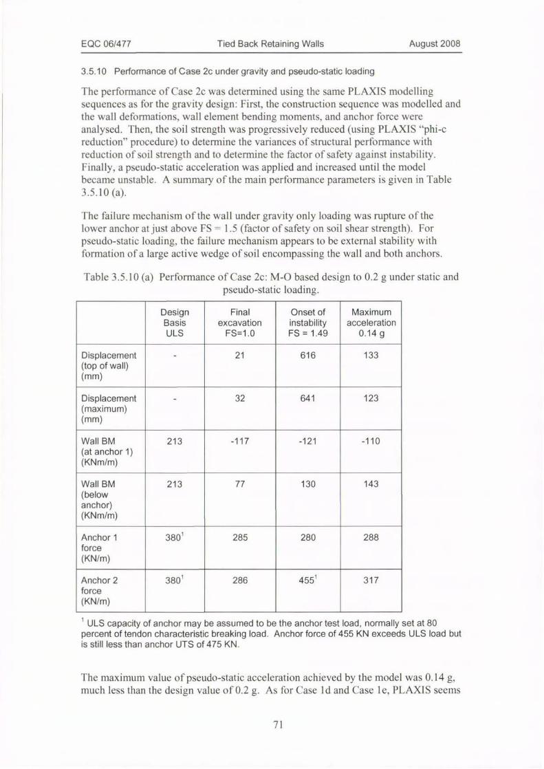
EQC 06/477 Tied Back Retaining Walls August 2008
3.5.10 Performance of Case 2c under gravity and pseudo-static loading
The performance of Case 2c was determined using the same PLAXIS modellingsequences as for the gravity design: First, the construction sequence was modelled andthe wall deformations. wall element bending moments, and anchor force were
analysed. Then, the soil strength was progressively reduced (using PLAXIS "phi-creduction" procedure) to determine the variances o f structural performance withreduction of soil strength and to determine the factor of safety against instability.Finally, a pseudo-static acceleration was applied and increased until the modelbecame unstable. A summary o f the main performance parameters is given in Table3.5.10 (a).
Fhe failure mechanism of the wall under gravity only loading was rupture of the
lower anchor at just above FS = 1.5 (factor of safety on soil shear strength). Forpseudo-static loading, the failure mechanism appears to be external stability withformation of a large active wedge of soil encompassing the wall and both anchors.
Table 3.5.10 (a) Performance of Case 2c: M-O based design to 0.2 g under static andpseudo-static loading.
Design Final Onset of Maximum
Basis excavation instability acceleration
ULS FS=1.0 FS = 1.49 0.14 g
Displacement - 21 616 133
(top of wall)(mm)
Displacement - 32 641 123
(maximum)(mm)
Wall BM 213 -117 -121 -110
(at anchor 1)(KNm/m)
Wall BM 213 77 130 143
(belowanchor)(KNm/m)
Anchorl 380
force
(KN/m)
1285 280 288
Anchor 2 380
force
(KN/m)
i 286 4551
317
1 ULS capacity of anchor may be assumed to be the anchor test load, normally set at 80percent of tendon characteristic breaking load. Anchor force of 455 KN exceeds ULS load butis still less than anchor UTS of 475 KN.
The maximum value of pseudo-static acceleration achieved by the model was 0.14 g,much less than the design value of 0.2 g. As for Case Id and Case le, PLAXIS seems
71

EQC 06/477 Tied Back Retaining Walls August 2008
unable to model large values of pseudo-static acceleration without generating deepseated shear failures through the entire soil deposit, as shown in Figure 3.5.10 (a).
1
- - 50>3 N
Figure 3.5.10 (a). Deep seated failure mechanism for Case 2c at horizontalacceleration of 0.14 g.
Performance of Case 2c under seismic loading
The performance of Case 2c under seismic loading was determined by applying onlyone scaled earthquake time-history record (Loma Prieta) to the PLAXIS model over arange of increasing PGA's: 0.2 g, 0.4 g, and 0.6 g. Results from all ofthe analysesfor the Case 2c are summarised in Figures 3.5.11 (a), (b). (c). and (d).
250 -
,
150
100
50 -
0
0 0.1 0.2 0.3 0.4 0.5 0.6 0.7
PGA (g)
Figure 3.ill (a). Accumulated wall crest displacement after I.oma Prieta earthquakefor 0.2 g design.
72
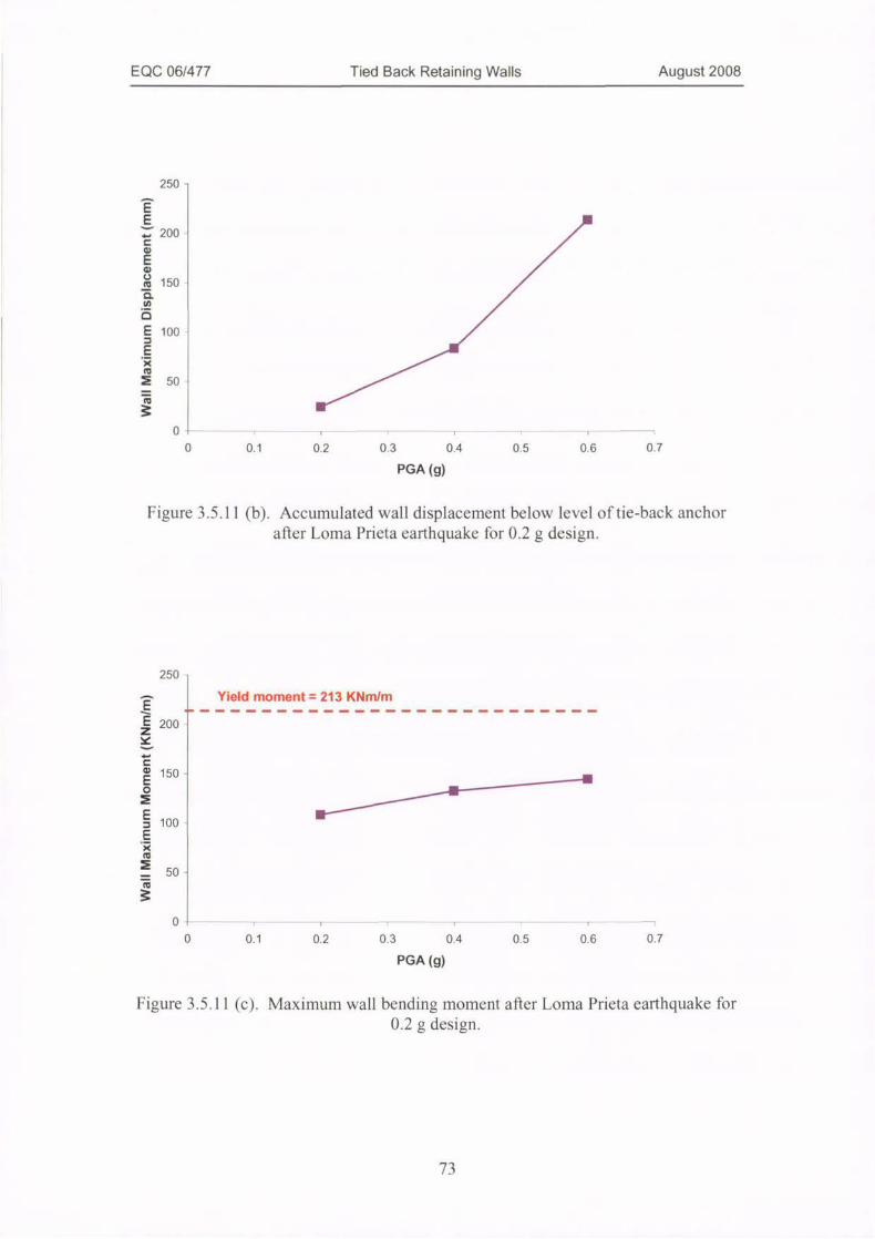
EQC 06/477 Tied Back Retaining Walls August 2008
250 -
200
150
100
50
0
0 0.1 0.2 0.3 0.4 0.5 0.6 0.7
PGA (g)
Figure 3.5.11 (b). Accumulated wall displacement below level oftie-back anchorafter I.oma Prieta earthquake for 0.2 g design.
250 -
Yield moment = 213 KNm/m
200 -
150 -
100
50 -
0 , , ,
0 0.1 0.2 0.3 0.4 0.5 0.6 0.7
PGA (g)
Figure 3.5.11 (c). Maximum wall bending moment after Loma Prieta earthquake for0.2 g design.
73
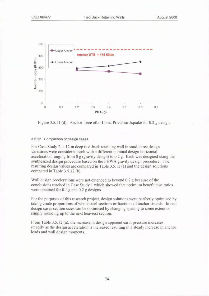
EQC 06/477 Tied Back Retaining Walls August 2008
500 -
--------------
--- Upper Anchor
400 - Anchor UTS = 475 KN/m
-+- Lower Anchor --0
300
200
100
0
0 0.1 0.2 0.3 0.4 0.5 0.6 0.7
PGA (g)
Figure 3.ill (d). Anchor force after Loma Prieta earthquake for 0.2 g design.
Comparison of design cases
For Case Study 2, a 12m deep tied-back retaining wall in sand, three design
variations were considered each with a different nominal design horizontalacceleration ranging from 0 g (gravity design) to 0.2 g. Each was designed using the
synthesized design procedure based on the FHWA gravity design procedure. 1 heresulting design values are compared in Table 3.5.12 (a) and the design solutionscompared in Table 3.5.12 (b).
Wall design accelerations were not extended to beyond 0.2 g because of theconclusions reached in Case Study 1 which showed that optimum benefit cost ratioswere obtained for 0.1 g and 0.2 g designs.
For the purposes of this research project. design solutions were perfectly optimised bytaking crude proportions of whole steel sections or fractions of anchor strands. In realdesign cases section sizes can be optimised by changing spacing to some extent orsimply rounding up to the next heaviest section.
From Table 3.5.12 (a), the increase in design apparent earth pressure increasessteadily as the design acceleration is increased resulting in a steady increase in anchorloads and wall design moments.
74

EQC 06/477 Tied Back Retaining Walls August 2008
Table 3.5.12 (a). Comparison of design values for case study Sand 2.
Design Parameter Case 2a Case 2b Case 2c
Design acceleration 0 g 0.1 g 0.2 g
Apparent earth pressure, p 42 51 61(KN/m2)
Anchor 1 design load (horizontal) 188 229 276
(KN/m)
Anchor 2 design load (horizontal) 185 224 271
(KN/m)
Base reaction 31 38 46
(KN/m)
Cantilever bending moment (at 91 110 133
anchor 1) (KNm/m)
Maximum bending moment (at 91 110 133
anchor 2) (KNm/m)
ULS design bending moment, M* 145 176 213
(KNm/m)
The design solutions for Case Study 2 are compared in Table 3.5.12 (b). The anchorand soldier pile sizes were optimised in an unrealistic way by taking proportions ofwhole member sizes. This optimisation was done to provide a more clear indicationof trends for the purposes of the study.
For Case Study 2, the anchor free lengths were determined as follows: The angle ofinclination of the M-0 active wedge slip plane was calculated for the nominal soilstrength. The anchor free lengths were extended to a line drawn from the toe of theembedded soldier piles to the ground surface at the calculated angle of inclination o fthe active slip plane. This approach is much simpler than that used in Case Study 1where the soil friction angle was reduced by the factor of safety calculated for internalstability. The benefit of using longer free-lengths (ilatter angle of inclination) wastested in Case Study 3 where the angle of inclination was flattened by five degrees.
75
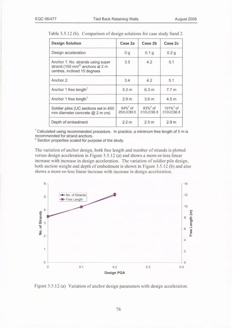
EQC 06/477 Tied Back Retaining Walls August 2008
Table 3.5.12 (b). Comparison of design solutions for case study Sand 2.
Design Solution Case 2a Case 2b Case 2c
Design acceleration 0 g 0.1 g 0.2 g
Anchor 1: No. strands using super 3.5 4.2 5.1
strand (100 mm anchors at 2 mcentres, inclined 15 degrees
Anchor 2: 3.4 4.2 5.1
Anchor 1 free lengthl 5.3 m 6.3 m 7.7 m
Anchor 1 free lengthl 2.9 m 3.6 m 4.5 m
Soldier piles (UC sections set in 450 94%2 of 83%2 of 101 %2 of
mm diameter concrete @2m crs) 250UC89.5 310UC96.8 310UC96.8
Depth of embedment 2.2 m 2.5 m 2.9 m
1 Calculated using recommended procedure. In practice, a minimum free length of 5 m isrecommended for strand anchors.
2 Section properties scaled for purpose of the study.
The variation of anchor design. both free length and number of strands is plottedversus design acceleration in Figure 3.5.12 (a) and shows a more-or-less linearincrease with increase in design acceleration. The variation of soldier pile design,both section weight and depth of embedment is shown in Figure 3.5.12 (b) and alsoshows a more-or-less linear increase with increase in design acceleration.
6- -14
5-0- No of Strands 12
--- Free Length
10
4
8
3
-6
2-
4
1--2
0 , · 0
0 0.1 0.2 0.3 0.4
Design PGA
Figure 3.5.12 (a) Variation of anchor design parameters with design acceleration.
76
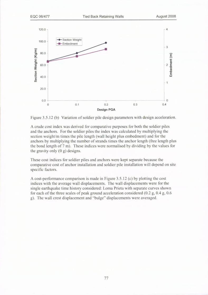
EQC 06/477 Tied Back Retaining Walls August 2008
120.0 - -4
100 0 - 20-Section Weight -- Embedment ---0-3
80.0 -
60.0 - 2
40.0 -
1
20.0 -
0.0 , 0
0 0.1 0.2 0.3 0.4
Design PGA
Figure 3.5.12 (b) Variation of soldier pile design parameters with design acceleration.
A crude cost index was derived for comparative purposes for both the soldier pilesand the anchors. For the soldier piles the index was calculated by multiplying thesection weight/m times the pile length (wall height plus embedment) and for theanchors by multiplying the number of strands times the anchor length (free length plusthe bond length of 7 m). These indices were normalised by dividing by the values forthe gravity only (0 g) designs.
These cost indices for soldier piles and anchors were kept separate because thecomparative cost of anchor installation and soldier pile installation will depend on sitespecific factors.
A cost-performance comparison is made in Figure 3.5.12 (c) by plotting the costindices with the average wall displacements. The wall displacements were for thesingle earthquake time history considered: Loma Prieta with separate curves shownfur each of the three scales of peak ground acceleration considered (0.2 g, 0.4 g, 0.6g). The wall crest displacement and "bulge" displacements were averaged.
77
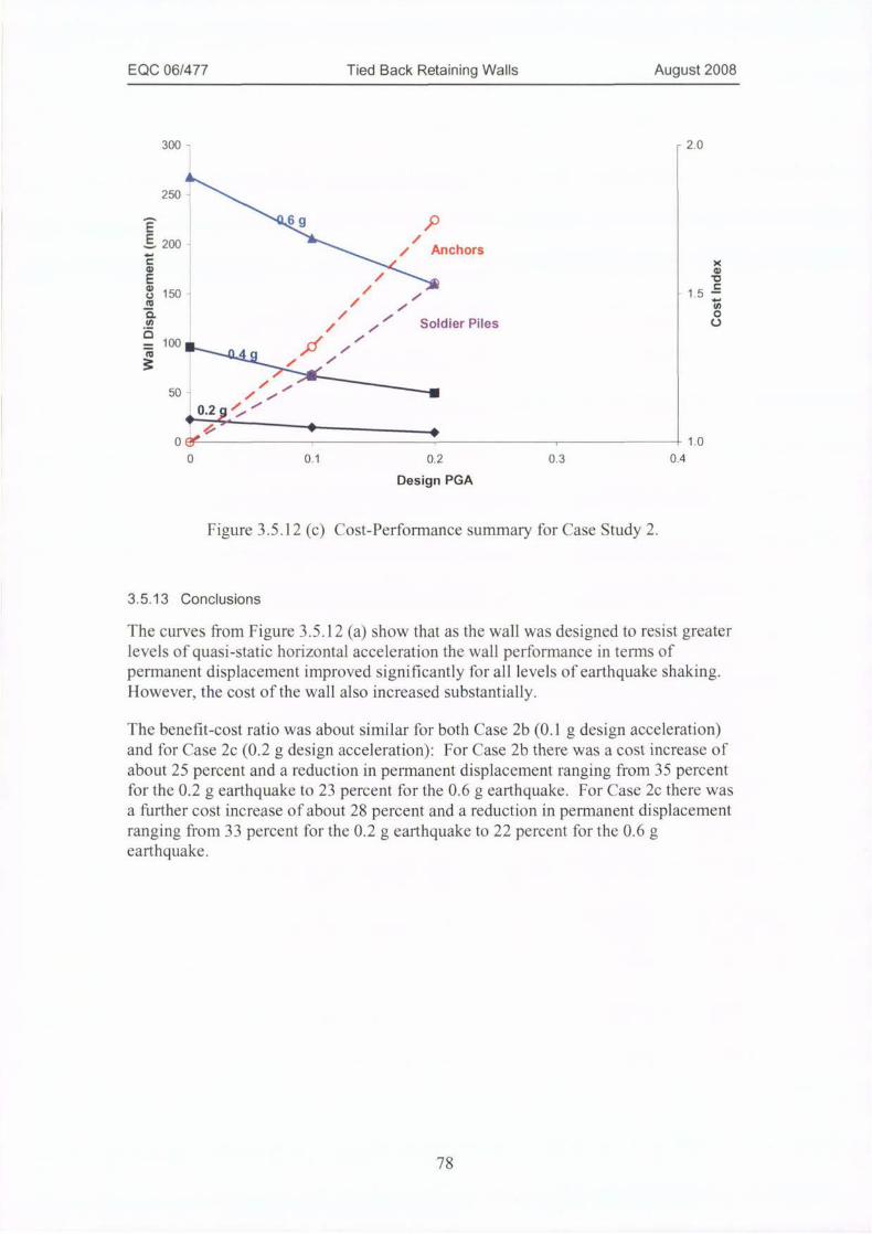
EQC 06/477 Tied Back Retaining Walls August 2008
300 - -2.0
250 -
-200-/ Anchors
i 150 -
L
100 I<
50 -
Soldier Piles
X
.g15 E
0
0
-0-4.2
,
1 ,I ,
////
0.2 gO'
Oe
0 0.1 0.2 0.3
1.0
0.4
Design PGA
Figure 3.5.12 (c) Cost-Performance summary for Case Study 2.
3.5.13 Conclusions
The curves from Figure 3.5.12 (a) show that as the wall was designed to resist greaterlevels of quasi-static horizontal acceleration the wall performance in terms ofpermanent displacement improved significantly for alllevels of earthquake shaking.However, the cost ofthe wall also increased substantially.
The benefit-cost ratio was about similar for both Case 2b (0.1 g design acceleration)and for Case 2c (0.2 g design acceleration): For Case 2b there was a cost increase ofabout 25 percent and a reduction in permanent displacement ranging from 35 percentfor the 0.2 g earthquake to 23 percent fur the 0.6 g earthquake. For Case 2c there wasa further cost increase ofabout 28 percent and a reduction in permanent displacement
ranging from 33 percent for the 0.2 g earthquake to 22 percent for the 0.6 gearthquake.
78
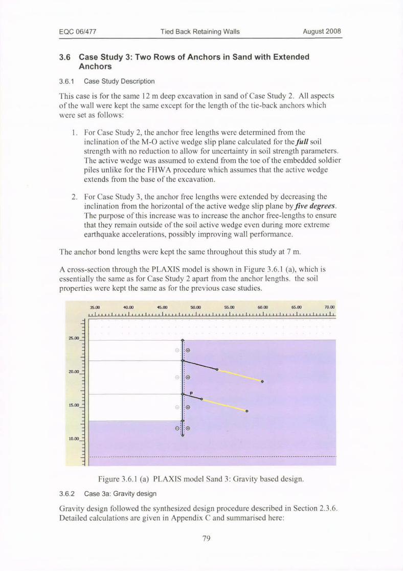
EQC 06/477 Tied Back Retaining Walls
3.6 Case Study 3: Two Rows of Anchors in Sand with ExtendedAnchors
3.6.1 Case Study Description
This case is for the same 12m deep excavation in sand of Case Study 2. All aspectsof the wall were kept the same except for the length of the tie-back anchors whichwere set as follows:
1. For Case Study 2, the anchor free lengths were determined from theinclination ofthe M-0 active wedge slip plane calculated for theA/U soilstrength with no reduction to allow for uncertainty in soil strength parameters.The active wedge was assumed to extend from the toe of the embedded soldierpiles unlike for the FLIWA procedure which assumes that the active wedgeextends from the base ofthe excavation.
2. For Case Study 3, the anchor free lengths were extended by decreasing theinclination from the horizontal ofthe active wedge slip plane by five degrees.
The purpose of this increase was to increase the anchor free-lengths to ensurethat they remain outside ofthe soil active wedge even during more extremeearthquake accelerations, possibly improving wall performance.
The anchor bond lengths were kept the same throughout this study at 7 m.
A cross-section through the PLAXIS model is shown in Figure 3.6.1 (a), which isessentially the same as for Case Study 2 apart from the anchor lengths. the soilproperties were kept the same as for the previous case studies.
35.00 40.00 45.00 50.00 55.00 60.00 65.00 70.00
/1ItII1II/1ll11/1III11I11I1I1/IllI11II1IIIlI1IIIlIII|1I1II11II|I111IIIII|1
25.00 -
191 0
20.00 -
P
15.00 -
10.00_=
Figure 3.6.1 (a) PLAXIS model Sand 3: Gravity based design.
3.6.2 Case 3a: Gravity design
Gravity design followed the synthesized design procedure described in Section 2.3.6.Detailed calculations are given in Appendix C and summarised here:
79

EQC 06/477 Tied Back Retaining Walls August 2008
Table 3.6.2 (a). Design values for case study Sand 3a: Gravity design.
Design Parameter Value
Apparent earth pressure, p 42 KN/m2
Anchor 1 design load (horizontal) 188 KN/m
Anchor 2 design load (horizontal) 185 KN/m
Base reaction 31 KN/m
Cantilever bending moment (at anchor 1) 91 KNm/m
Maximum bending moment (at anchor 2) 91 KNm/m
ULS design bending moment, M* 145 KNm/m
The wall structural elements were designed using these basic calculated design valuesas follows. For the purposes of this research project, design solutions were perfectlyoptimised, whereas for everyday design it would be necessary to select from standardproducts (e.g. standard anchor configurations, stock steel sections).
Table 3.6.2 (b). Design solutions for case study Sand 3a: Gravity design.
Design Solution Value
Anchor 1 cross-section (using super strandanchors at 2 m centres, inclined 15 degrees))
350 mm2 per anchor(3.5 strands per anchor)
Anchor 2 cross-section (using super strandanchors at 2 m centres, inclined 15 degrees))
344 mm2 per anchor(3.44 strands per anchor)
Anchor 1 free length 6.3
Anchor 2 free lengthl 3.5 m
Soldier piles (UC sections set in 450 mm 94%2 of 250UC89.5
diameter concrete @2m crs)
Depth of embedment 2.2 m
1 Calculated using FHWA procedure. In practice, a minimum free length of 5 m isrecommended for strand anchors.
2 Section properties scaled for purpose of the study.
The anchor free length for Case 3a was determined from the inclination ofthe M-0active wedge slip plane calculated for the jU 11 soil strength less jive degrees. Theactive wedge was assumed to extend from the toe of the embedded soldier piles unlikefor the FHWA procedure which assumes that the active wedge extends from the baseof the excavation.
The factor of safety against external stability was increased from 1.32 to 1.39 byincreasing the anchor free lengths (Table 3.6.2 (c)).
80
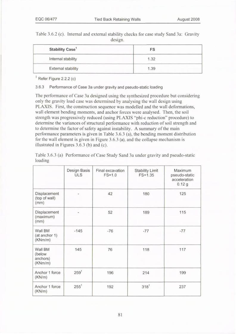
EQC 06/477 Tied Back Retaining Walls August 2008
Table 3.6.2 (c). Internal and external stability checks for case study Sand 3a: Gravitydesign.
1
Stability Casel FS
Internal stability 1.32
External stability 1.39
Refer Figure 2.2.2 (c)
3.6.3 Performance of Case 3a under gravity and pseudo-static loading
The performance o f Case 3a designed using the synthesized procedure but consideringonly the gravity load case was determined by analysing the wall design usingPLAXIS. First, the construction sequence was modelled and the wall deformations,wall element bending moments, and anchor forces were analysed. Then, the soilstrength was progressively reduced (using PLAXIS "phi-c reduction" procedure) todetermine the variances of structural performance with reduction of soil strength andto determine the factor of safety against instability. A summary of the mainperformance parameters is given in Table 3.6.3 (a),the bending moment distributionfur the wall element is given in Figure 3,6,3 (a), and the collapse mechanism isillustrated in Figures 3.6.3 (b) and (c).
rable 3.6.3 (a) Performance of Case Study Sand 3a under gravity and pseudo-staticloading
Design Basis Final excavation Stability Limit Maximum
ULS FS=1.0 FS=1.35 pseudo-staticacceleration
0.12g
Displacement - 42 180 125
(top of wall)(mm)
Displacement - 52 189 115
(maximum)(mm)
Wall BM -145 -76 -77 -77
(at anchor 1)(KNm/m)
Wall BM 145 76 118 117
(belowanchors)(KNm/m)
Anchor 1 force 259
(KN/m)
1196 214 199
Anchor 1 force 255
(KN/m)
1192 318
1237
81

EQC 06/477 Tied Back Retaining Walls August 2008
1 ULS capacity of anchor may be assumed to be the anchor test load, normally set at 80percent of tendon characteristic breaking load. Anchor load of 318 KN/m (100 percent ofcharacteristic breaking load) is limiting the final stability of the wall.
1 he collapse mechanism of the wall appears to be internal failure with rupture of thelower anchor.
3.6.4 Evaluation of Case 3a under gravity loading
I he factor of safuty achieved in the PLAXIS analysis using "phi-c reduction" (lowerbound) is greater than the value estimated using the limiting equilibrium, internalstability, wedge analysis and is considered satisfactory. Rupture of the lower anchoris an undesirable failure mechanism and results from increasing the anchor freelength.
It would be desirable to increase the anchor size to prevent this failure mode.
3.6.5 Performance of Case 3a under seismic loading
The performance of Case 3a, gravity only design, under seismic loading wasdetermined by applying only one scaled earthquake time-history record (Loma Prieta)to the PLAXIS model over a range of increasing PGA's: 0.2 g, 0.4 g, and 0.6 g. Thisrecord was determined from Case Study 1 to be much more critical than the otherearthquake time histories.
Wall performance is indicated primarily by permanent displacement (alwaysoutwards) remaining after each earthquake "event". For the wall of Case Study 3a,the displacement was maximum at either the crest or near to the base below the
second row of anchors where the wall typically tends to "bulge" outwards.
The bending moments in the wall elements were critical at either the top row ofanchors or below the second row of anchors (the "bulge") and these were alsomonitored together with the anchor forces. Results from all of the analyses for theCase 3a are summarised in Figures 3.6.5 (a), (b), (c), and (d).
82

EQC 06/477 Tied Back Retaining Walls August 2008
350
300
250 -
200 -
150 -
100
50
0
0 0.1 0.2 0.3 0.4 0.5 0.6 0.7
PGA (g)
Figure 3.6.5 (a). Accumulated wall crest displacement after Lorna Prieta earthquakefor gravity only design.
300
.250-
200
150
100
50
0
0 0.1 0.2 0.3 0.4 0.5 0.6 0.7
PGA (g)
Figure 3.6.5 (b). Accumulated wall displacement below level of tie-back anchor afterLoma Prieta earthquake for gravity only design.
83
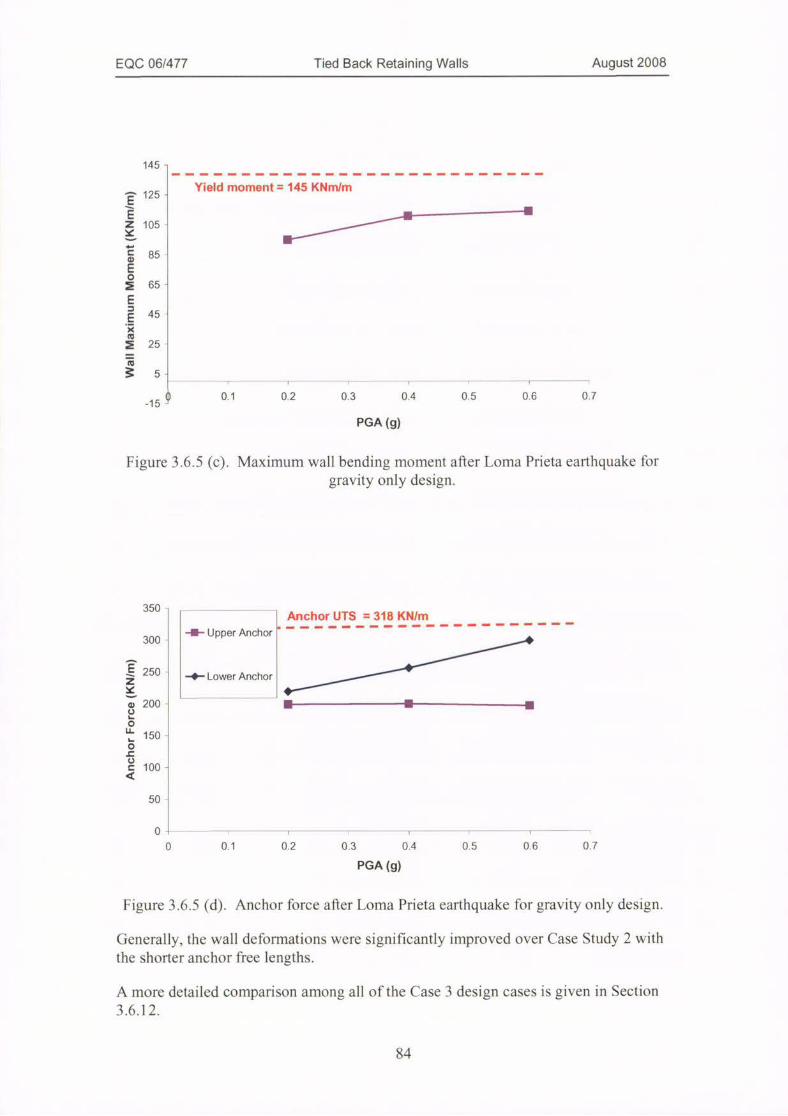
EQC 06/477 Tied Back Retaining Walls August 2008
145 -
Yield moment = 145 KNm/m· 125 -
105 -
85
65 -
45
25
5-1 1 1 1
0 0.1 0.2 0.3 0.4 0.5 0.6 0.7-15
PGA (g)
Figure 3.6.5 (c). Maximum wall bending moment after Loma Prieta earthquake forgravity only design.
350
300
Anchor UTS = 318 KN/m
0.-Upper Anchor - - - - ---- -- - -- - - - ---
250-0-Lower Anchor
200 I . I
150
100 -
50 ·
0
0 0.1 0.2 0.3 0.4 0.5 0.6 0.7
PGA (g)
Figure 3.6.5 (d). Anchor force after Loma Prieta earthquake for gravity only design.
Generally, the wall deformations were significantly improved over Case Study 2 withthe shorter anchor free lengths.
A more detailed comparison among all ofthe Case 3 design cases is given in Section
84
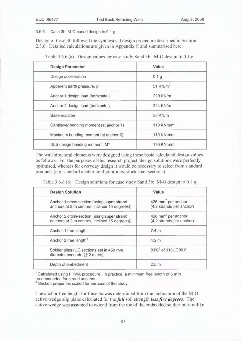
EQC 06/477 Tied Back Retaining Walls August 2008
3.6.6 Case 3b: M-O based design to 0.1 g
Design of Case 3b followed the synthesized design procedure described in Section2.3.6. Detailed calculations are given in Appendix C and summarised here:
Table 3.6.6 (a). Design values for case study Sand 3b: M-O design to 0.1 g.
Design Parameter Value
Design acceleration 0.1 g
Apparent earth pressure, p 51 KN/m2
Anchor 1 design load (horizontal) 229 KN/m
Anchor 2 design load (horizontal) 224 KN/m
Base reaction 38 KN/m
Cantilever bending moment (at anchor 1) 110 KNm/m
Maximum bending moment (at anchor 2) 110 KNm/m
ULS design bending moment, M* 176 KNm/m
The wall structural elements were designed using these basic calculated design valuesas follows. For the purposes of this research project, design solutions were perfectlyoptimised. whereas for everyday design it would be necessary to select from standardproducts (e.g. standard anchor configurations, stock steel sections).
Table 3.6.6 (b). Design solutions for case study Sand 3b: M-O design to 0.1 g.
Design Solution Value
Anchor 1 cross-section (using super strandanchors at 2 m centres, inclined 15 degrees))
426 mm2 per anchor(4.2 strands per anchor)
Anchor 2 cross-section (using super strandanchors at 2 m centres, inclined 15 degrees))
426 mm2 per anchor(4.2 strands per anchor)
Anchor 1 free length 7.4 m
Anchor 2 free lengthl 4.2 m
Soldier piles (UC sections set in 450 mm 83%
diameter concrete @2m crs)
2 of 310UC96.8
Depth of embedment 2.5 m
1 Calculated using FHWA procedure. In practice, a minimum free length of 5 m isrecommended for strand anchors.
2 Section properties scaled for purpose of the study.
Ihe anchor free length for Case 3a was determined from the inclination of the M-0active wedge slip plane calculated for the*// soil strength less jive degrees. Theactive wedge was assumed to extend from the toe of the embedded soldier piles unlike
85
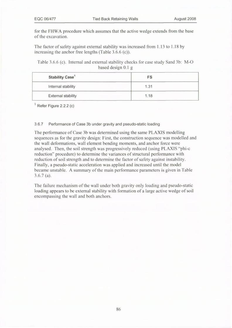
EQC 06/477 Tied Back Retaining Walls August 2008
fur the FHWA procedure which assumes that the active wedge extends from the baseof the excavation.
The factor of safety against external stability was increased from 1.13 to 1.18 byincreasing the anchor free lengths (Table 3.6.6 (c))
Table 3.6.6 (c). Internal and external stability checks for case study Sand 3b: M-Obased design 0.1 g
Stability Casel FS
Internal stability 1.31
External stability 1.18
Refer Figure 2.2.2 (c)
3.6.7 Performance of Case 3b under gravity and pseudo-static loading
The performance of Case 3b was determined using the same PLAXIS modellingsequences as for the gravity design: First, the construction sequence was modelled andthe wall deformations. wall element bending moments, and anchor force wereanalysed. Then, the soil strength was progressively reduced (using PLAXIS "phi-creduction" procedure) to determine the variances of structural performance withreduction of soil strength and to determine the factor of safety against instability.Finally. a pseudo-static acceleration was applied and increased until the modelbecame unstable. A summary of the main performance parameters is given in Table3.6.7 (a).
The failure mechanism of the wall under both gravity only loading and pseudo-staticloading appears to be external stability with formation of a large active wedge of soilencompassing the wall and both anchors.
86
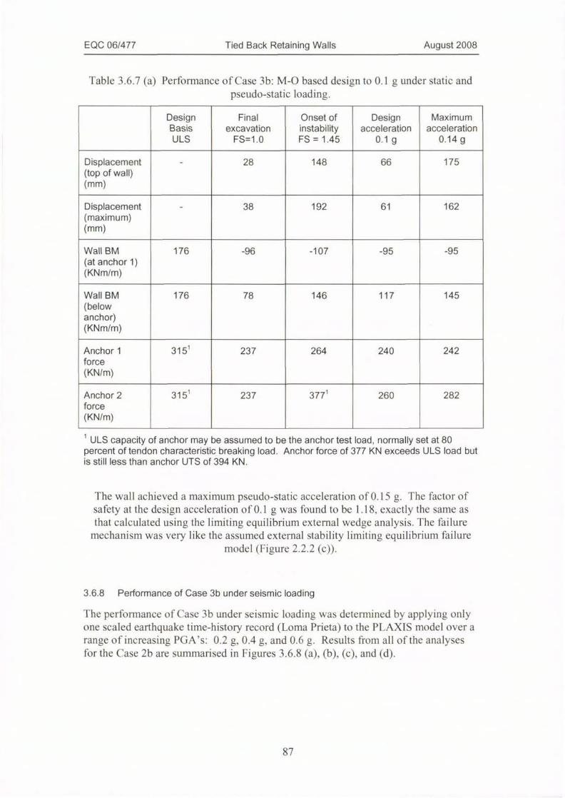
EQC 06/477 Tied Back Retaining Walls August 2008
Table 3.6.7 (a) Performance of Case 3b: M-O based design to 0.1 g under static andpseudo-static loading.
Design Final Onset of Design Maximum
Basis excavation instability acceleration acceleration
ULS FS=1.0 FS = 1.45 0.1 g 0.14 g
Displacement - 28 148 66 175(top of wall)(mm)
Displacement - 38 192 61 162(maximum)(mm)
Wall BM 176 -96 -107 -95 -95
(at anchor 1)(KNm/m)
Wall BM 176 78 146 117 145
(belowanchor)
(KNm/m)
Anchor 1 315
force
(KN/m)
1237 264 240 242
Anchor 2 3151force
(KN/m)
237 377 260 282
1 ULS capacity of anchor may be assumed to be the anchor test load, normally set at 80percent of tendon characteristic breaking load. Anchor force of 377 KN exceeds ULS load butis still less than anchor UTS of 394 KN.
The wall achieved a maximum pseudo-static acceleration of 0.15 g. 1 he factor ofsafety at the design acceleration of 0. 1 g was found to be 1.18 exactly the same asthat calculated using the limiting equilibrium external wedge analysis. The failure
mechanism was very like the assumed external stability limiting equilibrium failuremodel (Figure 2.2.2 (c)).
3.6.8 Performance of Case 3b under seismic loading
The performance of Case 3b under seismic loading was determined by applying onlyone scaled earthquake time-history record (Loma Prieta) to the PLAXIS model over arange o f increasing PGA's: 0.2 g, 0.4 g, and 0.6 g. Results from all of the analysesfor the Case 2b are summarised in Figures 3.6.8 (a), (b), (c). and (d).
87

EQC 06/477 Tied Back Retaining Walls August 2008
250
,
150 -
100 -
50
0
0 0.1 0.2 0.3 0.4 0.5 0.6 0.7
PGA (g)
Figure 3.6.8 (a). Accumulated wall crest displacement after Loma Prieta earthquakefor 0.1 g design.
250
200
150 -
100
50 -
0
0 0.1 0.2 0.3 0.4 0.5 0.6 0.7
PGA (g)
Figure 3.6.8 (b). Accumulated wall displacement below level of tie-back anchor afterLoma Prieta earthquake for 0.1 g design.
88
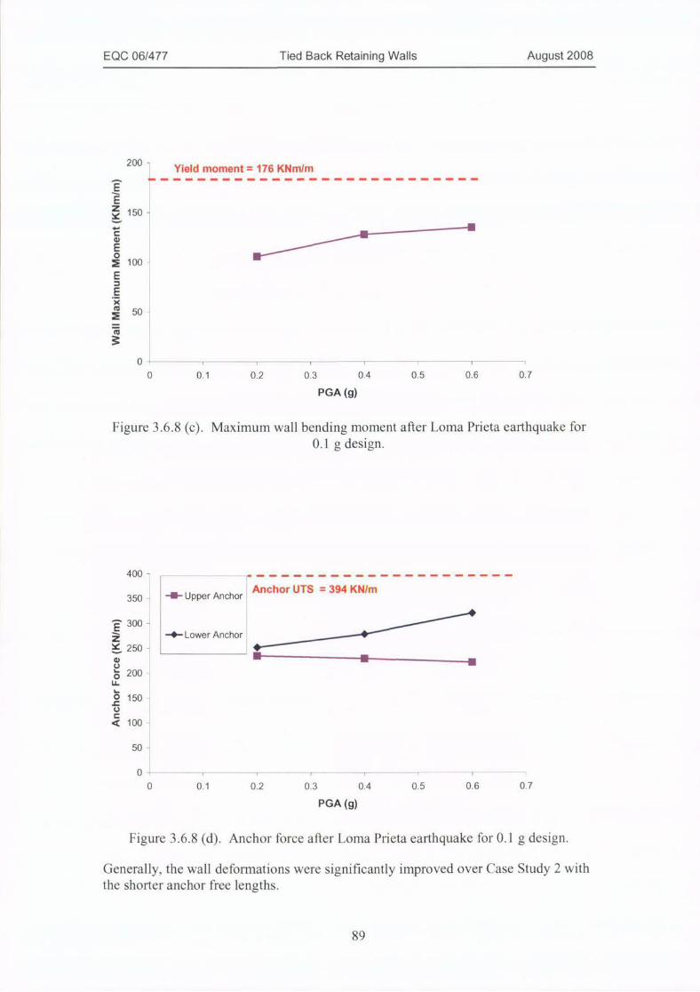
EQC 06/477 Tied Back Retaining Walls August 2008
200 -Yield moment = 176 KNrn/m
150 -
100 -
50 -
0
0 0.1 0.2 0.3 0.4 0.5 0.6 0.7
PGA (g)
Figure 3.6.8 (c). Maximum wall bending moment after I.oma Prieta earthquake for0.1 g design.
400 - --------------
Anchor UTS = 394 KN/m350 - -lF Upper Anchor
'300-
-0-Lower Anchor, --+0250-
200
150 -
100 -
50 -
0
0 0.1 0.2 0.3 0.4 0.5 0.6 0.7
PGA (g)
Figure 3.6.8 (d). Anchor force after Loma Prieta earthquake for 0.1 g design.
Generally, the wall deformations were significantly improved over Case Study 2 withthe shorter anchor free lengths.
89
EQC 06/477 Tied Back Retaining Walls August 2008
A more detailed comparison among all of the Case 3 design cases is given in Section3.6.12.
3.6.9 Case 30: M-O based design to 0.2 g
Design of Case 3c followed the synthesized design procedure described in Section2.3.6. Detailed calculations are given in Appendix B and summarised here:
Table 3.6.9 (a). Design values for case study Sand 3c: M-O design to 0.2 g.
Design Parameter Value
Design acceleration 0.2 g
Apparent earth pressure, p 61 KN/mz
Anchor 1 design load (horizontal) 276 KN/m
Anchor 2 design load (horizontal) 271 KN/m
Base reaction 46 KN/m
Cantilever bending moment (at anchor 1) 133 KNm/m
Maximum bending moment (at anchor 2) 133 KNm/m
ULS design bending moment, M* 213 KNm/m
The wall structural elements were designed using these basic calculated design values
as follows. For the purposes of this research project, design solutions were perfectlyoptimised, whereas for everyday design it would be necessary to select from standardproducts (e.g. standard anchor configurations. stock steel sections).
Table 3.6.9 (b). Design solutions for case study Sand 3c: M-O design to 0.2 g.
Design Solution Value
Anchor 1 cross-section (using super strandanchors at 2 m centres, inclined 15 degrees))
514 mm2 per anchor(5.1 strands per anchor)
Anchor 2 cross-section (using super strandanchors at 2 m centres, inclined 15 degrees))
514 mm2 per anchor(5.1 strands per anchor)
Anchor 1 free length 8.7 m
Anchor 2 free lengthl 5.1 m
Soldier piles (UC sections set in 450 mmdiameter concrete @2m crs)
101%2 of 310UC96.8
Depth of embedment 2.9 m
1 Calculated using FHWA procedure. In practice, a minimum free length of 5 m isrecommended for strand anchors.
2 Section properties scaled for purpose of the study.
90

EQC 06/477 Tied Back Retaining Walls August 2008
The anchor free length for Case 30 was determined from the inclination of the M-Oactive wedge slip plane calculated for thefi,// soil strength less five degrees. Theactive wedge was assumed to extend from the toe of the embedded soldier piles unlikefor the FHWA procedure which assumes that the active wedge extends from the baseof the excavation.
The factor of safety against external stability was increased from 1.00 to 1.04 byincreasing the anchor free lengths (Table 3.6.2 (c)).
Table 3.6.9 (c). Internal and external stability checks for case study Sand 30: M-0based design 0.2 g
Stability Casel FS
Internal stability 1.26
External stability 1.04
Refer Figure 2.2.2 (c)
3.6.10 Performance of Case 3c under gravity and pseudo-static loading
The performance of Case 2c was determined using the same PLAXIS modellingsequences as for the gravity design: First, the construction sequence was modelled andthe wall deformations, wall element bending moments, and anchor force wereanalysed. Then, the soil strength was progressively reduced (using PLAXIS "phi-creduction" procedure) to determine the variances of structural performance withreduction of soil strength and to determine the factor of safety against instability.Finally. a pseudo-static acceleration was applied and increased until the modelbecame unstable. A summary of the main performance parameters is given in Table3.6.10 (a).
The failure mechanism of the wall under gravity only loading was by the externalstability mechanism. For pseudo-static loading, the failure mechanism appears to beexternal stability with formation of a large active wedge of soil encompassing the walland both anchors.
The maximum value of pseudo-static acceleration achieved by the model was 0.18 g,less than the design value of 0.2 g. As for Case k PLAXIS seems unable to modellarge values of pseudo-static acceleration without generating deep seated shearfailures through the entire soil deposit, as shown in Figure 3.5.10 (a).
91
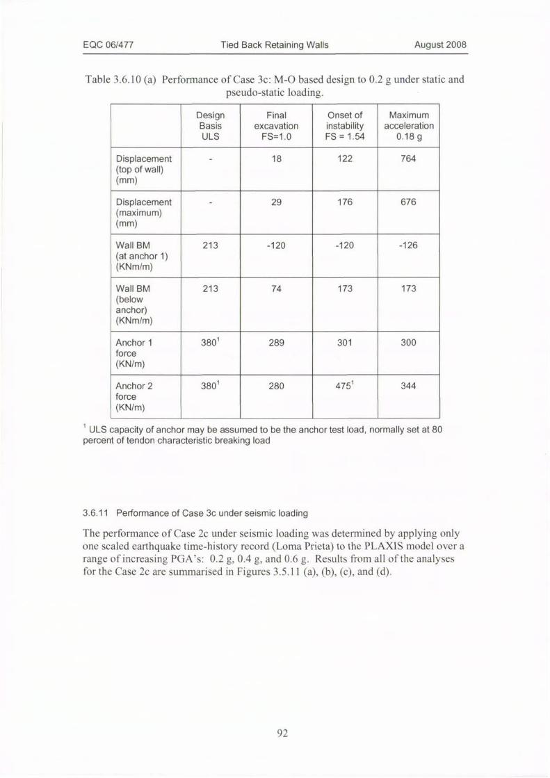
EQC 06/477 Tied Back Retaining Walls August 2008
Table 3.6.10 (a) Performance of Case 3c: M-O based design to 0.2 g under static andpseudo-static loading.
Design Final Onset of Maximum
Basis excavation instability acceleration
ULS FS=1.0 FS = 1.54 0.18g
Displacement - 18 122 764
(top of wall)(mm)
Displacement - 29 176 676
(maximum)(mm)
Wall BM 213 -120 -120 -126
(at anchor 1)(KNm/m)
Wall BM 213 74 173 173
(belowanchor)(KNm/m)
Anchorl 380
force
(KN/m)
1289 301 300
Anchor 2 380
force
(KN/m)
1280 475i 344
1 ULS capacity of anchor may be assumed to be the anchor test load, normally set at 80percent of tendon characteristic breaking load
3.6.11 Performance of Case 3c under seismic loading
The performance of Case 2c under seismic loading was determined by applying onlyone scaled earthquake time-history record (Loma Prieta) to the PLAXlS model over a
range of increasing PGA's: 0.2 g. 0.4 g, and 0.6 g. Results from all ofthe analysesfur the Case 2c are summarised in Figures 3.5.11 (a), (b), (c), and (d).
92
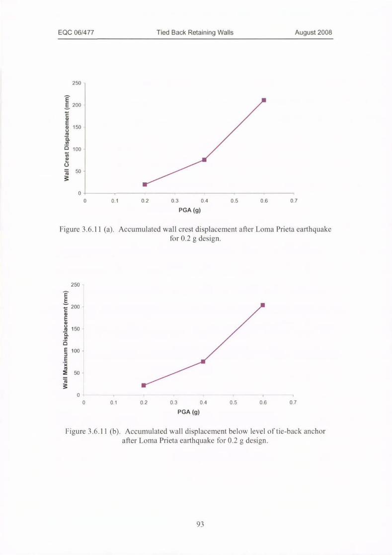
EQC 06/477 Tied Back Retaining Walls August 2008
250
150
100
50 -
0
0 0.1 0.2 0.3 0.4 0.5 0.6 0.7
PGA (g)
Figure 3.6.11 (a). Accumulated wall crest displacement after Loma Prieta earthquakefor 0.2 g design.
250
'200 -
150 -
50 -
i i r 1 1
0 0.1 0.2 0.3 0.4 0.5 0.6 0.7
PGA (g)
Figure 3.6.11 (b). Accumulated wall displacement below level of tie-back anchor
after Loma Prieta earthquake for 0.2 g design.
93

EQC 06/477 Tied Back Retaining Walls August 2008
250 -
Yield moment = 213 KNm/m
200 - -
150 -
100 -
50 -
0
0 0.1 0.2 0.3 0.4 0.5 0.6 0.7
PGA (g)
Figure 3.6.11 (c). Maximum wall bending moment after Lorna Prieta earthquake for0.2 g design.
500 -
I.-Upper AnchorAnchor UTS = 475 KN/m
400 -
-O- Lower Anchor ,---A
' 300
200 -
100 -
0
0 0.1 0.2 0.3 0.4 0.5 0.6 0.7
PGA (g)
Figure 3.6.11 (d). Anchor force after Loma Prieta earthquake for 0.2 g design.
94
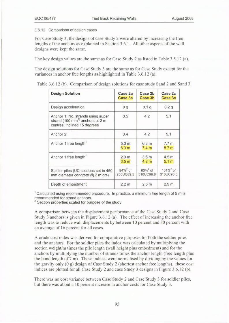
EQC 06/477 Tied Back Retaining Walls August 2008
3.6.12 Comparison of design cases
For Case Study 3. the designs ofcase Study 2 were altered by increasing the freelengths of the anchors as explained in Section 3.6.1. All other aspects of the wall
designs were kept the same.
The key design values are the same as for Case Study 2 as listed in Table 3.5.12 (a).
The design solutions for Case Study 3 are the same as for Case Study except for thevariances in anchor free lengths as highlighted in Table 3.6.12 (a).
Table 3.6.12 (b). Comparison of design solutions for case study Sand 2 and Sand 3.
Design Solution Case 2a Case 2b Case 2c
Case 3a Case 3b Case 3c
Design acceleration 0 g 0.1 g 0.2 g
Anchor 1: No. strands using super 3.5 4.2 5.1
strand (100 mm2 anchors at 2 mcentres, inclined 15 degrees
Anchor 2: 3.4 4.2 5.1
Anchor 1 free length1
5.3 m 6.3 m 7.7 m
6.3 m 7.4 m 8.7 m
Anchor 1 free length1
2.9 m 3.6 m 4.5 m
3.5 m 4.2 m 5.1 m
Soldier piles (UC sections set in 450 94%2 of 83%2 of 101 %2 of
mm diameter concrete @2m crs) 250UC89.5 310UC96.8 310UC96.8
Depth of embedment 2.2 m 2.5 m 2.9 m
1 Calculated using recommended procedure. In practice, a minimum free length of 5 m isrecommended for strand anchors.
2 Section properties scaled for purpose of the study.
A comparison between the displacement performance of the Case Study 2 and CaseStudy 3 anchors is given in Figure 3.6.12 (a). The effect of increasing the anchor freelength was to reduce wall displacements by between 10 percent and 30 percent with
an average of 16 percent for all cases.
A crude cost index was derived for comparative purposes for both the soldier piles
and the anchors. For the soldier piles the index was calculated by multiplying thesection weight/m times the pile length (wall height plus embedment) and for the
anchors by multiplying the number of strands times the anchor length ( free length plusthe bond length of 7 m). These indices were normalised by dividing by the values forthe gravity only (0 g) design of Case Study 2 (shortest anchor free lengths). these costindices are plotted for all Case Study 2 and case Study 3 designs in Figure 3.6.12 (b).
There was no cost variance between Case Study 2 and Case Study 3 for soldier liles,but there was about a 10 percent increase in anchor costs for Case Study 3.
95
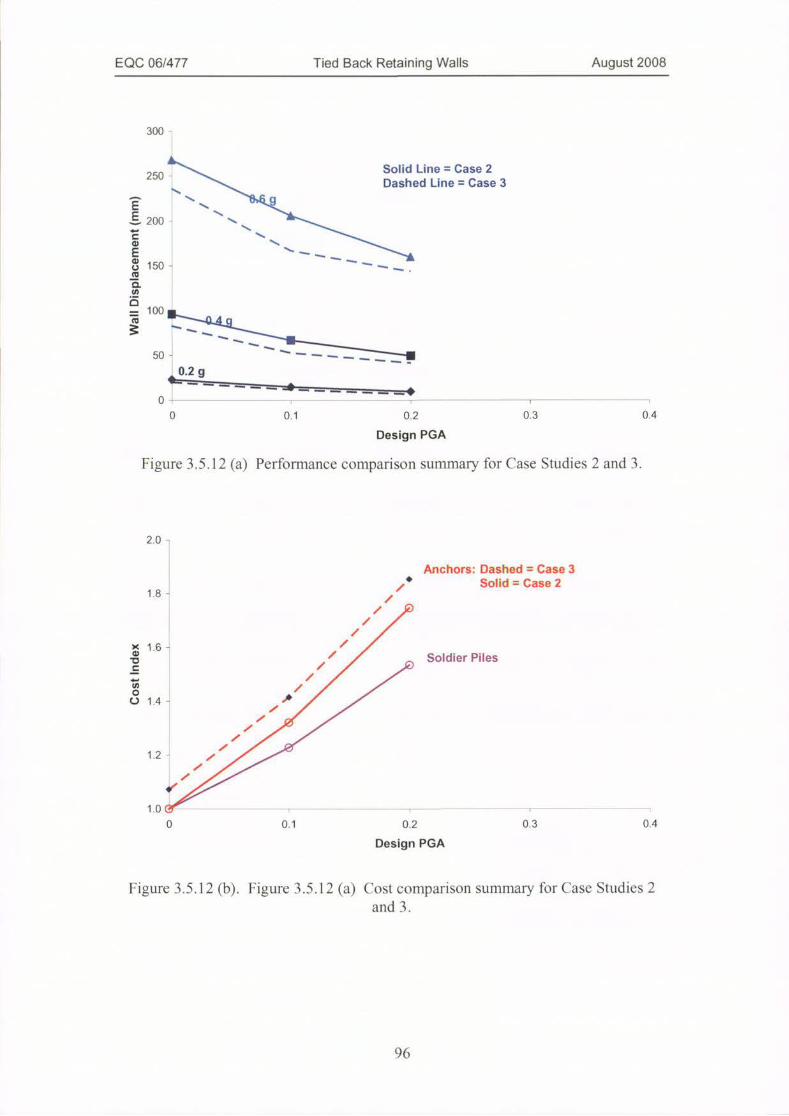
EQC 06/477 Tied Back Retaining Walls August 2008
3001
250 - Solid Line = Case 2
Dashed Line = Case 3
200 -
--------150 -
100.
50 - --- - 22210.2 g
0
0 0.1 0.2 0.3 0.4
Design PGA
Figure 3.5.12 (a) Performance comparison summary for Case Studies 2 and 3.
2.0 -
1.8 -
Anchors: Dashed = Case 3
Solid = Case 2
1.6 -4 1 Soldier Piles
1 1
14-0
* 4
:r,1.2 -
100 0.1 0.2 0.3 0.4
Design PGA
Figure 3.5.12 (b). Figure 3.5.12 (a) Cost comparison summary for Case Studies 2and 3.
96
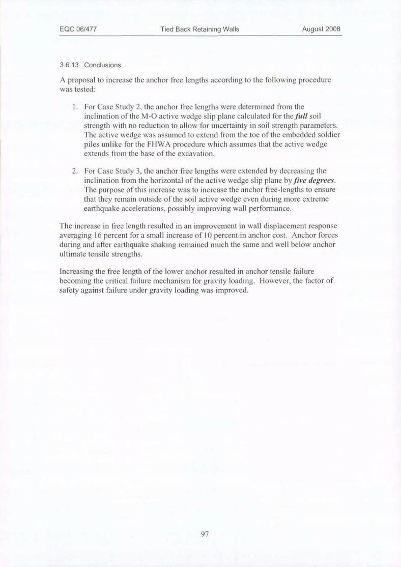
EQC 06/477 Tied Back Retaining Walls August 2008
3.6.13 Conclusions
A proposal to increase the anchor free lengths according to the following procedurewas tested:
1. For Case Study 2, the anchor free lengths were determined from theinclination of the M-0 active wedge slip plane calculated for thefi,// soilstrength with no reduction to allow for uncertainty in soil strength parameters.The active wedge was assumed to extend from the toe of the embedded soldierpiles unlike for the FHWA procedure which assumes that the active wedgeextends from the base of the excavation.
2. For Case Study 3, the anchor free lengths were extended by decreasing theinclination from the horizontal of the active wedge slip plane by.five degrees.The purpose ofthis increase was to increase the anchor free-lengths to ensurethat they remain outside of the soil active wedge even during more extremeearthquake accelerations, possibly improving wall performance.
The increase in free length resulted in an improvement in wall displacement response
averaging 16 percent for a small increase of 10 percent in anchor cost. Anchor forcesduring and after earthquake shaking remained much the same and well below anchorultimate tensile strengths.
Increasing the free length of the lower anchor resulted in anchor tensile failure
becoming the critical failure mechanism for gravity loading. However, the factor ofsafety against failure under gravity loading was improved.
97
EQC 06/477 Tied Back Retaining Walls August 2008
4 Design Guidelines
4.1 Overview
One of the main objectives for this study was to develop workable design guidelinesfor use by practicing engineers. As such they need to be as simple as possible withoutoverlooking or over-simplifying key aspects of performance or safety of tied-backwalls.
The approach adopted has been to build on an existing design procedure that is wellproven and in wide use: The apparent earth pressure diagrams of Terzaghi and Peck[1967] subsequently updated, revised, and re-published in the FHWA GeoteclinicalEngineering Circular No. 4. [Sabatini. et. al., 1999].
This study has investigated several aspects of the performance of tied-back wallsdesigned using the FHWA including the factor of safety against instability undergravity loads as well as the seismic performance. This study has shown that theFHWA design procedure is sound, at least for the case studies examined, but proposessome minor improvements and clarifications to the procedure as follows:
1. The line for setting the anchor free-lengths should extend from the embeddedbase of the wall, not from the base of the excavation. The reason for this
recommendation is that the PLAXIS analysis indicates that active soil failuresurfaces that develop pass below the embedded portions of the wall. The bondzone of the anchors should be placed outside ofthe active soil wedge. (Thisapproach was used in all of the case studies in this report).
2. Further, it is recommended that the assumed angle of inclination of the activewedge should be calculated using the Mononobe-Okabe theory [Okabe, 1926;Mononobe and Matsuo, 1929]. An additional flattening by five degrees isrecommended to provide some "buffer" against variability and uncertainty insoil parameters and to improve the seismic performance.
3. The depth of embedment of soldier piles or continuous wall elements shouldbe calculated using Broms's [1965] theory with a factor of safety of 3. Theprocedure for calculating depth of embedment is not clearly stated in the
FHWA procedure. A factor of safety of 3 when using Broms's theory tocalculate passive lateral resistance of piles is commonly recommendedbecause of the large deformations required to generate passive soil resistance.
4. Final checks of wall designs should be made using limiting equilibriummethods to verify both the internal and external stability. This process is
alluded to in the FHWA report but no clear guidance is given. (Detailedexample calculations for the case studies are appended to this report.)
The recommendations given in this report are based on detailed analysis of a limitednumber of case studies with greatly simplified soil conditions and so should beconsidered tentative.
98
EQC 06/477 Tied Back Retaining Walls August 2008
No consideration is given in the recommended design procedure for directlyconsidering the likely deformations. The limited case study analyses indicate thatdeformations will be "reasonable" for many situations. Of course "reasonableness" ofdeformation will depend very much on the particular context of each individual wallbeing designed. The designer must consider which situations will be more critical todeformation and carry out appropriate analysis.
4.2 Seismic Design Accelerations
The proposed design procedure for tied-back retaining walls is based on a "pseudo-static" approach where the equilibrium ofthe structure and internal stresses areassessed considering a static horizontal component of acceleration in addition togravity. Generally, it is uneconomic or even impracticable to design walls to resistvery high values of "quasi-static" acceleration. Instead, reduced values ofacceleration, as of 1/3 to 1/2 the design peak ground acceleration, are considered [e.g.Kramer, 1996].
The rationale for using such low design values of horizontal acceleration is that thePGA occurs only for brief instants of time (in the millisecond range) during anearthquake. The soil mass is considered to behave in a "ductile" fashion - yieldingbrietly during these peaks with little accumulation of strain or strain-softening effects.The structural elements of the wall do not, in general, feel the effect of the momentarypeak accelerations and respond mainly to the soil deformations.
In general, the lower the value of the selected "pseudo-static" acceleration, the greaterwill be the de formation of the wall and retained soil after an earthquake. However, animportant conclusion from this study is that substantial reductions of deformationwere found when walls were designed to resist even modest levels of pseudo-staticacceleration (as low as 0.1 g). Further reductions in deformation with increasinglevels of design acceleration were observed but became increasingly modest as thedesign acceleration was increased. Even when walls were designed to resist the fullpeak ground accelerations (100 percent of PGA) significant deformations stilloccurred.
Based on the results of this study and previous published recommendations, thefollowing recommendations are made for minimum design accelerations for tied-backretaining walls:
1. Tied-back walls should be designed to resist a minimum pseudo-statichorizontal acceleration of 0.1 g. This value is considered a sensible minimumvalue and was shown in this study to give very good improvements inearthquake performance for a modest increase in wall cost. As an additionalbenefit, the factor of safety against instability under gravity loading is alsoincreased.
2. For higher seismic hazard zones or for structures of greater importance, tied-back walls should be designed to resist a minimum pseudo-static accelerationof 1/3 PGA to th PGA of the design earthquake.
99

EQC 06/477 Tied Back Retaining Walls August 2008
Where deformations are critical it may be necessary to use still higher values ofpseudo-static acceleration. However, it rapidly becomes impractical to design wallsto resist very high accelerations and it appears impossible to reduce deformationsbelow certain limits.
4.3 Proposed Design Guidelines for "Sand" soils
The following is a detailed recommendation for designing tied-back retaining walls in"sand" soils. Examples of the calculations are given for the case studies in theAppendices.
a) Initial trial geometry: The depth of excavation and depth to each row ofanchors needs to be estimated as a first step, based on experience or trial anderror.
b) Prepare apparent earth pressure diagram: As shown in Figure 4.3 (a).Note that KA is calculated using the Mononobe-Okabe equation with theselected design pseudo-static acceleration. The wall is assumed to befrietionless (i.e. the wall is likely to move downwards with any active soilwedge).
c) Calculate anchor design load(s): As shown in Figure 4.3 (a).
d) Calculate wall base reaction, lt: As shown in Figure 4.3 (a).
e) Calculate wall section bending moment: From the apparent earth pressure
diagram as shown in Figure 4.3 (b). These methods are considered to provideconservative estimates ofthe calculated bending moments, but may not
accurately predict the specific locations of the maximum. FHWA
recommends an allowable stress of Fb - 0.55 Fy for steel soldier piles. ForNew Zealand design procedures using load and resistance factor design
(LRFD) principles and for a strength reduction factor for steel sections of 0.8,an equivalent load factor of a = 0.8/0.55 - 1.45 is implied. However, for
consistency with NZS 4203 a load factor of 1.6 is recommended for the
purpose of sizing wall structural elements. ('Ihis procedure was found to besuitably conservative for the case studies in this report).
f) Determine depth of embedment: Calculate required depth ofembedment forsoldier Files to resist wall base reaction (R) using Broms [19651 (but
calculating Kp using the Mononobe-Okabe equations including the designacceleration), or, for continuous walls using passive resistance fromMononobe-Okabe theory. A strength reduction factor of 3 is recommended tobe applied to these calculations because of the large plastic strains required tomobilise the full passive resistance.
g) Check internal stability of the wall: A possible internal failure mechanismis shown in Figure 4.3 (c), with an active failure wedge immediately behind
the wall, a passive wedge immediately in front of the embedded toe of thewall, and the anchor(s) developing their ultimate capacity (taken to be the
100

EQC 06/477 Tied Back Retaining Walls August 2008
proven, test capacity, normally 1.33 times the design load or 80 percent of theanchor tensile capacity).
The true factor of safety may be determined by progressively reducing the
assumed soil strength in the calculations until the driving and resisting forces
are just equal, i.e:
Active force = Passive force + anchor ultimate force
when the factor of safety against sliding is given by:
FStan '(0)
tan 1 (0,-ehic·ed
For the earthquake load case using pseudo-static design, a minimum factor of
safety of 1.2 is recommended, but not less than the factor of safety against
external stability.
h) Set "free"length of anchor tendons: The "free" length of the anchor
tendons should extend beyond the active soil wedge defined by theMononobe-Okabe theory flattened by five degrees, originating at the base of
the wall or the embedded soldier piles as indicated in Figure 4.3 (c).
i) Check external stability of the wall: External stability of tied-back retaining
walls in cohesionless soil is controlled by horizontal sliding of the wall with
formation of an active soil wedge behind the wall and a passive wedge in frontof the wall base, as shown in Figure 4.3 (c). The critical failure surface is
assumed to pass immediately behind the anchor bond zone, as shown.
For the earthquake load case using pseudo-static design, a mininium "true"
factor of safety of 1.1 based on mobilised soil shear strength is recommended.
j) Note: When calculating passive soil resistance, the interface friction angleshould be set to be no more than ¢/2. Use of higher values is not
recommended because the resulting values of passive resistance will be
unrealistically high.
101

EQC 06/477 Tied Back Retaining Walls August 2008
k A 1 A
2/3 H 1
Th 1
. 1/3 H
Th2
Thn
2/3 H 1
T •hl
H A
A
H1
H2 P
Hn
l
2/3 (H-H 1)
22 R R
1
2/3 Hn.
P=TOTAL LOAD
-KAYH P=TOTAL LOAD
2/3 H H -1/3 Hi- 1/3 H,+1
(a) Walls with one levelof ground anchors
(b) Walls with multiple levelsof ground anchors
Figure 4.3 (a). Apparent earth pressure diagram for cohesionless soils.
A
k . A k.H Hl
1
T
T
1 MB1
T
H
- ©MB \F2 BC
H P TCG< . 2 1 m T2uH 12,H
H BC Hnep.2 MCDM/6*1 D ITn & Tnu
Hn+1 MDE,/'' J TnL
In¥ /. E
MB = IMB MB = IMBMac= Maximum moment between B and C; Mc =MD=ME= 0
located at point where shear = 0M BC = Maximum moment between B and C;
located at point where shear = 0
MeD . MDE . Calculated as for MBC
(a) Walls with one level of ground anchors (b) Walls with multiple levels of ground anchors
Figure 4.3 (b). Estimation of wall element bending moments.
102
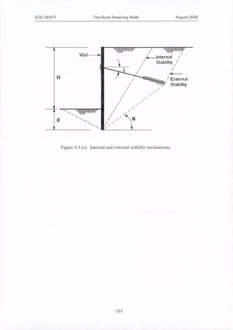
EQC 06/477 Tied Back Retaining Walls August 2008
Wall-----,
H
I f
d
14--Internal /
' Stability ,/t
/iS**: / External1 -7 Stability
jt
Figure 4.3 (c). Internal and external stability mechanisms.
103

EQC 06/477 Tied Back Retaining Walls August 2008
5 Summary and Conclusions
Very little guidance is available for the design of tied-back retaining walls to resistearthquake shaking. Little observational data on the behaviour of tied-back wallsduring earthquakes has been published, but, what there is suggests that they behavewell.
A survey of New Zealand practice has showed that there is no consistency ofapproach and that most designers are relying on a range of different "black box"computer software with earthquake loading input simply as an additional horizontalforce applied directly to the wall. The appropriateness of this approach isquestionable because the full range of different failure modes is not necessarilyaddressed by the software nor is it always obvious what the software does.
Methods for calculating the input additional earthquake "loading" on the wall alsowere found to vary from the lower bound, Mononobe-Okabe approach ( a variation ofCoulomb's method for calculating static loads on retaining walls) where the soil isassumed to be in a fully yielding "Rankine" state to the upper bound Wood approachwhere the wall is assumed to be rigid and the soil to remain fully elastic.
The commonly used software packages do not give guidance as to the length ofanchors required, especially the "free length" of the anchors. This study has shownthat the anchor lengths are very important in determining the wall response and thatthey should be lengthened as the design acceleration of the wall increases.
The focus of this study has been to develop a pragmatic, practical design procedurethat produces safe and economical designs and that does not depend on "black box"software. As a starting point, a well established design procedure for tied-backretaining walls under gravity loading was adopted (FHWA procedure, based on thesemi-empirical "apparent earth pressure" method of Terzaghi and Peck) and verifiedfor different, simplified case studies, using PLAXIS finite element analysis software.The analyses showed that this design procedure produced walls with adequate, but notexcessive, factors ofsafety against instability (FS = 1.38 for Case Study 1,7 m highwall with one row of anchors, FS = 1.32 for Case Study 2,12 m high wall with tworows of anchors).
The case studies assumed a generic, uniform "sand" soil with average propertiesmodelled in PLAXIS using the hardening soil model.
These standard, gravity designs then were subjected to simulated eat-thquakes, scaledto different values ofpeak ground acceleration (PGA = 0.2 g to 0.6 g) by usingnumerical time history analysis. The walls performed surprisingly well consideringthat they were not specifically designed to resist earthquakes: Wall displacementsbecame quite significant (worst case of 35() mm for the 7 m high wall under LomaPrieta record scaled to 0.6 g) for the extreme earthquake "events", but, the wallsremained stable, anchor forces remained well within acceptable limits, and the soldierpiles only reached yield in one case (7 m high wall, Loma Prieta record scaled to 0.6g).
104
EQC 06/477 Tied Back Retaining Walls August 2008
The PLAXIS time histories showed that the structural elements were little affected by
the high peak ground accelerations. Anchor forces generally varied little during theearthquakes, and showed little or no response to the large instantaneous variation inground acceleration, even for the very high peaks. Instead, anchor forces seemed torespond more to the gross deformations ofthe soil mass, either increasing slightly, or,
in some case, decreasing. Likewise, soldier pile bending moments showed littleresponse to the instantaneous variation in ground acceleration but showed a more
steady increase in bending moment towards the base of the wall as the grossdeformation of the soil mass increased during an earthquake.
Given the good performance of the walls designed using the gravity only FHWAprocedure, it was decided to use this procedure as the basis for an earthquake designprocedure. The FHWA document recommends the use ofthe pseudo-static
Mononobe-Okabe theory to design tied-back walls to resist earthquakes but does notgive a detailed procedure. Nor is such a procedure obvious because the recommendeddesign procedure for tied-back walls under gravity loading is based on the semi-empirical "apparent earth pressure" diagrams o f Terzaghi and Peck. However, forsands the apparent earth pressure is assumed to be proportional to Ka, the Rankineactive earth pressure and it was assumed that the equivalent apparent earth pressurefor the earthquake design case might be proportional to Kali, the Mononobe-Okabe
value for active earth pressure.
Of equal importance was the evident need to also extend the anchor free-lengths to
beyond the active soil zone immediately behind the wall. The Mononobe-Okabe
theory also provides a means for calculating the location of the active zone.
A new design procedure was synthesized from the FHWA procedure incorporatingthe use of the Mononobe-Okabe theory. The case study walls then were re-designedusing the new procedure for various design accelerations from 0.1 g to 0.4 g and
tested by running them through the same PLAXIS numerical earthquake simulations.Significant improvements in performance, reductions in wall deformation mainly,
were observed even for walls designed to resist low acceleration (0.1 g).
As walls were designed to resist greater levels of horizontal acceleration, wall
displacements continued to reduce, but at a decreasing rate. Even when a wall was
designed to resist 100 percent ofthe PGA of an earthquake, it still accumulated
significant permanent displacement by the end of the shaking.
There was a great range in wall displacements among the three different earthquake
records modelled (Loma Prieta, Parkfield, Sierra Madre), with variations of as much
as 300 percent.
The greatest benefit-cost ratio was found for the walls designed to resist the low level
(().1 g) accelerations. The additional cost of building the case study walls to resist 0.1
g was modest (about 25 percent) for a good reduction in wall deformation (about 30percent). The cost of increasing resistance beyond 0.2 g starts to increase very rapidlywith only modest reductions in wall deformation observed.
Designing walls to resist even a low level of acceleration (0.1 g) had the additional
benefit of significantly increasing the factor safety against instability for gravity
loading.
105
EQC 06/477 Tied Back Retaining Walls August 2008
The benefit-cost ratios established for the 7 m high wall (Case Stduy 1) indicate thatthe optimum design is probably gained by making the design acceleration about M thePGA of the design earthquake (e.g. for design earthquake with PGA = 0.2 g make thedesign acceleration 0.1 g, and for a design earthquake with PGA = 0.4 g make thedesign acceleration 0.2 g). Such a recommendation would be in keeping withaccepted practice which is to design retaining walls to resisit pseudo-staticacceleration of between M and 1/3 of the design earthquake PGA.
For the higher, 12 m walls, the study showed similar trends, although the benefit-costratio was about the same for walls designed to resist 0.1 g and 0.2 g horizontalacceleration.
The effect of increasing the anchor free length to beyond the active wedge slip plane(tlattening the slip plane by five degrees) was studied for 12 m high walls in CaseStudy 3. The increase in anchor free length resulted in an improvement in walldisplacement response averaging 16 percent for a small increase of 10 percent inanchor cost. Anchor forces during and after earthquake shaking remained much thesame and well below anchor ultimate tensile strengths.
Increasing the free length of the lower anchor resulted in anchor tensile failurebecoming the critical failure mechanism for gravity loading. However, the factor ofsafety against failure under gravity loading was improved.
This study has demonstrated that use of the PLAXIS finite element software with thedynamic analysis module is a useful tool for studying the performance of tied-backretaining walls and, probably, other complex problems in soil-structure interaction.The only difficulty experienced with the software was the inability to analyse deepexcavations under high pseudo-static accelerations. However, this is not considered aserious limitation since such situations are some what artificial and divorced from
practical reality.
This study has considered a limited range of case studies, and for walls greater in
height then the 12m considered, it is strongly recommended that a special study usingPLAXIS analysis or similar be considered during the design process. The trends fromthe case studies in this report suggest that as walls get higher, the factors of safetyreduce and the safety ofthe proposed design procedure has not been confirmed forsuch extrapolations.
A detailed, recommended design procedure for design oftied-back retaining wallswith earthquake loading is given in Section 4. This recommended procedure is basedon detailed analysis of a limited number of case studies with greatly simplified soilconditions and so should be considered tentative. On the other hand, it is based
closely on a well proven gravity design procedure.
No consideration is given in the recommended design procedure for directlyconsidering the likely deformations during shaking. The limited case study analysesindicate that deformations will be "reasonable" for many situations. Of course
"reasonableness" of deformation will depend very much on the particular context ofeach individual wall being designed. The designer must consider which situationswill be more critical to deformation and carry out appropriate analysis.
1()6
EQC 06/477 Tied Back Retaining Walls August 2008
It is recommended that walls should be designed to resist a minimum pseudo-staticacceleration of().1 g. Based on the case studies, this level ofacceleration was shownto give a good improvement in wall performance for only a modest increase in cost.The factor of safety against failure under gravity loading was also shown to be
significantly enhanced.
Little benefit was found from designing walls to resist the maximum peak groundacceleration (PGA) for a given earthquake: The improvements in wall performance
were found to become more modest once the design acceleration exceeded about 0.2
g. Even when walls were designed to resist 100 percent of the earthquake PGA,
significant wall deformations still occurred.
Attempts to design tied-back retaining walls to resist very high levels of horizontal
acceleration become difficult in any case.
The observations by Ho et. al. 11991] of little damage to tied- back retaining walls isunderstandable given the conclusions from this study: The walls studied herein were
found to be robust even when not specifically designed to resist earthquake shaking.
The observation of Fragaszy et. al. [1987] that wall elements extending into thefoundation soils may be subjected to very high bending moments is not supported bythis study. Adequate depth of embedment for all the wall studied was found to be acritical aspect of wall performance since it governs both the internal and externalstability o f a wall. Walls embedded into stiff soils but supporting softer soils may
expect to have more severe concentrations of bending at the interface but this was not
explored in this present study.
Sabatini et. al [ 1999] recommended that brittle elements ofthe wall system,
specifically the grout tendon bond should be governed by the peak ground
acceleration. This present study has shown that anchor forces are little affected byeven very high peak ground accelerations and normal anchor detailing and testing
should be adequate.
Most researchers to date have focused on calculating a "pressure" to be applied to
walts arising from the earthquake shaking, perhaps failing to view the wall aiid soilmass response in a holistic way. The results of this study indicate that there are
complex interactions between the retained soil mass and the wall elements that
contribute to a greater then expected resilience for walls but at the expense ofdeformations that seem impossible to reduce below certain levels.
107
EQC 06/477 Tied Back Retaining Walls August 2008
6 Recommendations for Future Research
The recommendations given in this report are based on detailed analysis of a limited
number of case studies with greatly simplified soil conditions. The effect of varying
soil conditions such as soft retained soil overlying a much stiffer foundation needfurther investigation.
Also, the study should be extended to look at higher walls. As walls increase in
height their complexity increases because of the need for multiple rows of anchors.They also become more flexible (relatively) and there will be more kinematic
interaction with incoming seismic waves during earthquakes.
The case studies considered were for steel soldier pile walls and the results areconsidered applicable to reinforced concrete soldier pile walls, continuous concretewalls, and also to steel sheet pile walls. Timber poles are also commonly used for
tied-back retaining walls of moderate height and require specific consideration
because of their more limited ductility.
Great variances in wall displacement were observed for the different earthquake timehistory records considered in this study. It would be useful to understand the reasons
for those variances so that it is possible to better predict wall deformation.
108
EQC 06/477 Tied Back Retaining Walls August 2008
References
Brinkgreve, R.B.G. and Vermeer, P.A. (1988). PLAXIS.finite element codefor soiland rock analyses, Version 7, Balkema, Rotterdam.
Broms, B.B. (1965). "Design of Laterally Loaded Piles." Journal of the Soil
Mechanics and Foundations Division, ASCE, Vol. 91, No. SM3, Proceedings Paper4342, pp. 79-99.
Frangaszy, R.J., Ali, A., Denby, G., and Kilian, A.P. (1987). "Seismic response oftieback walls," Transportation Research Record, Transportation Research Board,
Washington D.C.
Gaba, A. R., Simpson, B., Powrie, W., and Beadman, D. R. (2003) "Embeddedretaining walls - guidance for economic design," CIRIA C580, CIRIA London, 390 p.
Ho, C.L., Denby, G.M., and Fragaszy, R.J. (1990). "Sesimic performanceoftied-backwalls," Proceedings, ASCE Specialty Conference on Design and Performance ofEarth Retaining Structures, Geotechnical Specialty Publication No. 25, pp. 843-853.
Kramer, S.L. (1996). Geotechnical Earthquake Engineering, Prentice Hall, NewJersey, 653 p.
Mononobe, N. and Matsuo, H. (1929). "On the determination of earth pressuresduring earthquakes," Prciceedings, World Engineering Congress, 9p.
Okabe, S. (1926). "General theory of earth pressures," Journal of the Japan Society ofCivil Engineering, Vol. 12, No. 1.
Peck, R.B. (1969). "Deep Excavations and Tunneling in Soft Ground, State of ArtReport." Proceedings of the 7th International Conference on Soil Mechanics andFoundation Engineering, Mexico City, Mexico, pp. 225-290.
Sabatini, P.J., Pass, D.G., and Bachus, R.C. (1999). "Ground anchors and anchoredsystems," Geotechnical Circular No. 4, FHWA-IF-99-015, Federal Highway
Administration, Department of Transportation, Washington DC.
Siller, T.J. and Dolly, M.O. (1992). "Design of tied-back walls for seismic loading,"Journal o#Geotechnical Engineering, ASCE, Vol. 118, No. 11, pp. 1804-1821.
Siller, T.J. and Frawley, D.D. (1992). "Seismic response of multi anchored retainingwalls,"Journal 0/ Geotechnical Engineering, ASCE, Vol. 118, No. 11, pp. 1787-1803.
Siller, T.J., Christiano, P. P. & Bielak, 1 (1987). "On the dynamic behavior of tied-back retaining walls", Developments in Geotechnical Engineering Vol. 45; Structuresand Stochastic Methods [Selected Papers Presented at the 3rd InternationalConference on Soil Dynamics and Earthquake Engineering.]Elsevier SciencePublishers B.V. and Computational Mechanics Publications, Amsterdam andSouthampton, England, pp. 141.
109

EQC 06/477 Tied Back Retaining Walls August 2008
Siller, T.J., Christiano, P. & Bielak, J. (1991). "Seismic response oftied-back
retaining walls", Earthquake Engineering & Structural Dynamics, vol. 20, no. 7, pp.605-620.
-4 1
Terzaghi, K. and Peck, R.B. (1967). Soil Mechanics in Engineering Practice, z . Ed.,Wiley, New York, 729 p.
Wood, J. (1973). "Earthquake-induced soil pressures on structures," Report EERL 73-
05, California Institute of Technology, Pasadena, California, 311 p.
110

EQC 06/477 Tied Back Retaining Walls August 2008
Appendix A
A.1 Design calculations for case study Sand la - Gravity baseddesign
1. Calculation of Ka
horizontal acceleration in g 0 :=alan (kh) 0 =0B:= 0· deg slope of the back of the wall
i:= 0. deg slope of the backfill
¢ := 35·deg angle of internal friction
ji:= 0 angle of interface friction
Calculation
r sin* + 6·sin(0 -0-o r 2D := 1 +I , , , D- 2.476
cos(6i +P+oj costi -p),
Kcos 61)-0- p)2
AE- K
cos (0) cos (p )2 cos p + 6i + 0·DAE-
0.271
Equivalent Horizontal Component
KAEI-1 := cosi KAE KAF.El = 0.271
2. Calculation of apparent earth pressure
(Refer to Figure 2.2.2 (a). Units = KN/m2)
Hwall:= 7 Height of wallH 1 := 2 Distance to anchor
KA := 0.271
y:= 16
2 Load = 138.102Load := 0.65·KA'Y·Hwall1.oad
P:= p = 29.5780.667·H
wall
3. Calculation of anchor design load and reaction force required at base of wall.
111
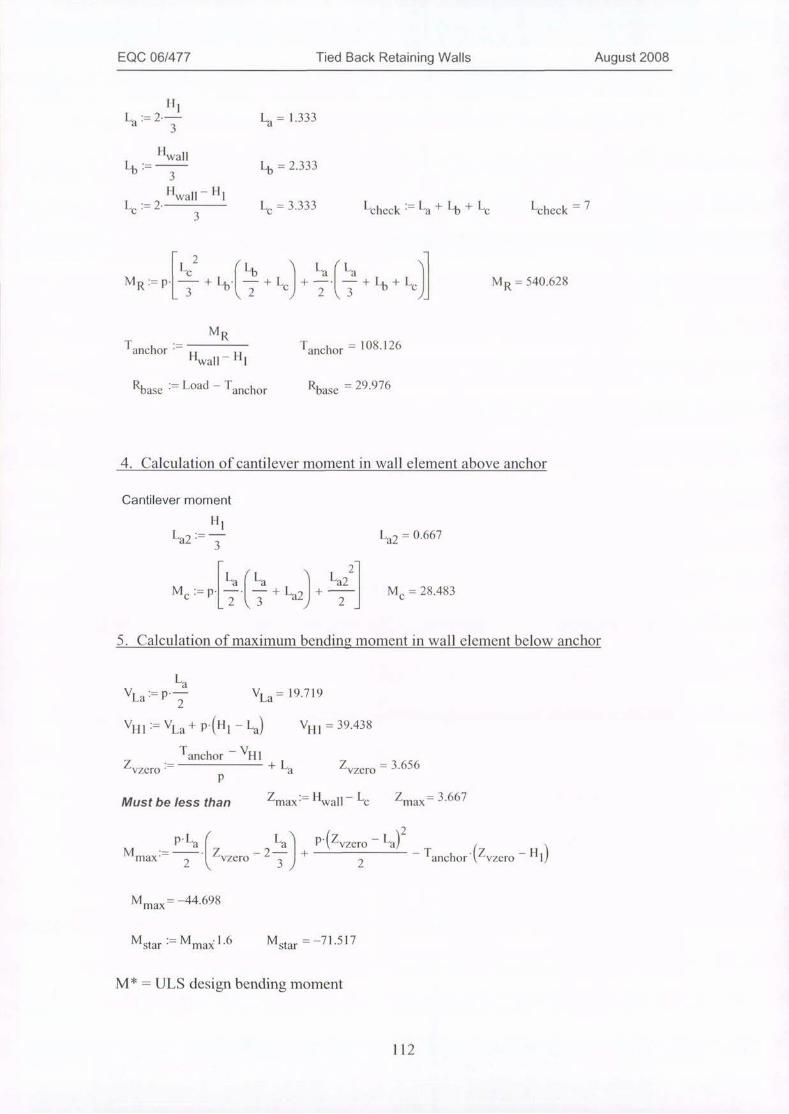
EQC 06/477 Tied Back Retaining Walls August 2008
H 1La r= 2.-3 La = 1.333
H
Lb:= -
1 '-2
wall
3
Hwall- H
3
Lb = 2.333
1
4 = 3.333 4heck = La + Lb + Le Lcheck 7
MR > P -
2
t
3
/ Lb-+L
2C 1 + 9 - C -41 +4+4 MR-= 540.628
MR1-anchor = 11 wall - H]
Tanchor = 108.126
Rbase = Load - Tanchor Rbase = 29.976
4. Calculation of cantilever moment in wall element above anchor
Cantilever moment
IllLa2 - - La2 - 0·667
3
Mc I Plit.132(3
2
+ La +- M2C
= 28.483
5. Calculation of maximum bending moment in wall element below anchor
VLa
La>P'V VLa -19.719
VH := VI-a + P Hl - La VHl = 39.438
anchor
P
-V
Z
T
vzero
H1+L
aZ
vzero= 3.656
Must be less than Zmax:= Hwall- Le Z = 3.667niax
- 2 P-(Zvzero
2
Mmax'
z -liz
2 lvzero
-Tanchor (Z
vzero-H 1J
Mmax- -44.698
M star *.- Mmax 1.6 Mstar =-71.517
M * = ULS design bending moment
112
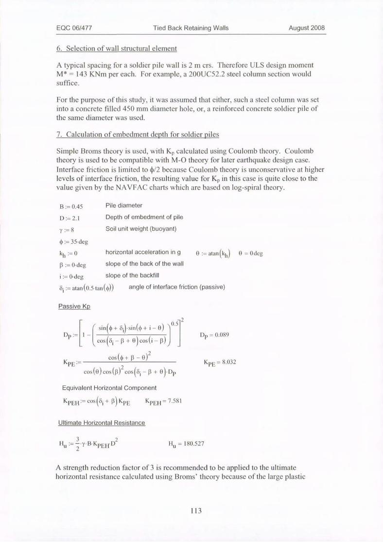
EQC 06/477 Tied Back Retaining Walls August 2008
6. Selection of wall structural element
A typical spacing for a soldier pile wall is 2 m crs. Therefore ULS design momentM* = 143 KNm per each. For example, a 200UC52.2 steel column section wouldsuffice.
For the purpose of this study, it was assumed that either, such a steel column was setinto a concrete filled 45() mm diameter hole, or, a reinforced concrete soldier pile ofthe same diameter was used.
7. Calculation of embedment depth for soldier piles
Simple Broms theory is used, with Kp calculated using Coulomb theory. Coulombtheory is used to be compatible with M-0 theory for later earthquake design case.
Interface friction is limited to ¢/2 because Coulomb theory is unconservative at higherlevels of interface friction, the resulting value for Kp in this case is quite close to thevalue given by the NAVFAC charts which are based on log-spiral theory.
B := 0.45 Pile diameter
D:= 2.1 Depth of embedment of pile
7:-8 Soil unit weight (buoyant)
*:=35·deg
kh:= 0 horizontal acceleration in g 0 := atan(kh)B:= 0·deg slope of the back of the wall
i:= 0·deg slope of the backfill
4 := atan 0.5- tan (*)) angle of interface friction (passive)
0 = Odeg
Passive Kp
-2/ i \ i . .()5
Dp:=_1 -cos@i-p + ())codi - 13) _sin<¢ + 6i)·sinbl)+ i - 0 JD
P=
KCos(0 +P-0)
PE.-
cos(O) cos(p)2 cos8i -
2
B + 0)·DK
P
PE -8.032
Equivalent Horizontal Component
KPE[' 2==cosi+ 13KPE KPEH= 7.581
Ultimate Horizontal Resistance
H3
u:=2 7.B·KPEH D2
1111
= 180.527
A strength reduction factor of 3 is recommended to be applied to the ultimate
horizontal resistance calculated using Broms' theory because ofthe large plastic
113

EQC 06/477 Tied Back Retaining Walls August 2008
strains required to mobilise full passive resistance. Therefore, for piles spaced at 2 mcentres:
Design Resistance =180/3 = 60 KN each pile or 30 KN/m run
Design Demand (Rbase) =30 KN/m
Therefore, embedment depth of 2.1 m is optimum.
8. Check for internal stability
(True FS determined by successive reduction of 0 j
Wall --+1
H
t
1a
.*Ar.
4--Internal /
' Stability,/1 11 1-
* 1 External
2'' Stabilityf
t
t
i
97
d
114
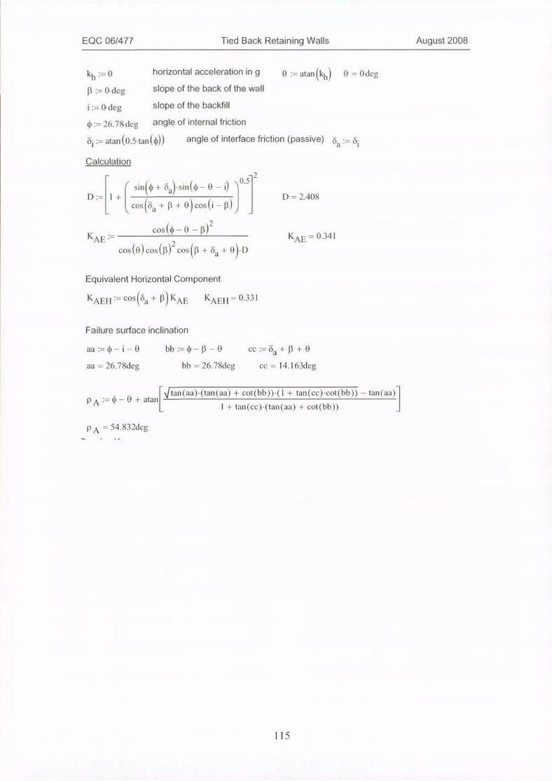
EQC 06/477 Tied Back Retaining Walls August 2008
kh:= 0 horizontal acceleration in g 8 := atan (kh)B:= 0-deg slope of the back of the wall
i:= 0·deg slope of the backfill
1):= 26.78deg angle of internal friction
4 := atan(0.5-tan(0)) angle of interface friction (passive) 6
0=
·= 6a·
0 deg
Calculation
r sin4) + Oa·sin(* -0 -i) 0.5 2D.= 1 +
L cos 6a + #+ 0 cos(i - 13) D = 2.408
cos (0 -0- 0)2KAE = KAE -0.341
cos(0)cos(13)ZcosB + 6a + 0*D
Equivalent Horizontal Component
KAE]-1 -cos tia + PKAE KArl 1 - 0.331
Failure surface inclination
aa:= 0-i-0 bb:=¢-B-0 ec:=ba +B+aa = 26.78deg bb = 26.78deg ce = 14.163deg
PA:-0-0 + atan+an(aa)·(tan(aa) + cot(bb))·(1 + tan(cc)·cot(bb)) - tan(aa)-1
1 + tan(cc)·(tan(aa) + cot(bb))
PA =54.832deg
115
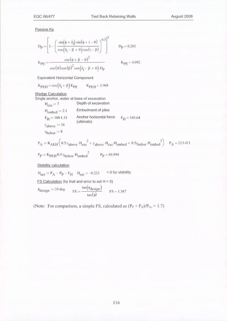
EQC 06/477 Tied Back Retaining Walls August 2008
Passive Kp
r sin((1) + bij·sin((1) +i-0) ju.5 2Dp:= 1-1 . / Dp = 0.201C cos Coi -P+ 0) cos(i -13))KpE:=
i2
cos(0+13-0)
cos<0)cos([1)2 cosoi -P+ 0·1)K
P
PE-4.092
Equivalent Horizontal Component
KPEH := cos tii + [1 KpE KpEH = 3.968
Wedqe Calculation
Single anchor, water at base of excavation
Hexc = 7 Depth of excavation
Hembed = 2.1 Embedment of piles
FH := 108.1,33
Fabove * 1 6
Anchor horizontal force F
(ultimate)H
= 143.64
l'below ' 8
2PA := KAEI-1-(O5.yabove Hexc + Yabove Hexc'Hembed + 57below+'embed PA = 213.411
2
PP := KPE' f 0.5.ybelow Hembed Pp = 69.994
Stabilitv calculation
' 'net = PA - PP - Fll Hnet = -0.223 < 0 for stability
FS Calculation (by trial and error to set H = 0)
design = 35·deg tall(bdeslgnFS := FS = 1.387
tan<(1)
(Note: For comparison, a simple FS, calculated as (Pp + FH)/PA, = 1.7)
116
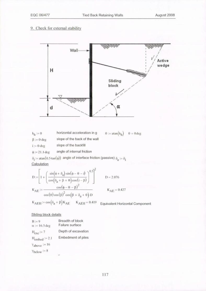
EQC 06/477 Tied Back Retaining Walls August 2008
9. Check for external stability
A
Wail- -
H
I U
d
Slidintblock
t
0 := atan h
7f
0 = 0 deg
11VJ
kh:= 0 horizontal acceleration in g , ch)B :=0· deg slope of the back of the wall
i:= 0. deg slope of the backfill
¢:=21.1·deg angle of internal friction
bi - atan(0.5-tan(0)) angle of interface friction (passive) tia := tiiCalculation
21 ' 0.5
r sin1) + tia) sin(0 -0-i)D:= 1+I .1 D = 2.076
l cos (da + 13 + 0) COS (i - B)
Kcos (0 -0- p)2
AE= K
cos(())cos(B) cos[3 + 6a+ 0) DAE -
0.427
1<Ali] 1 -= cosba + KAE KAEH - 0.419 Equivalent Horizontal Component
Sliding block details
13:= 9 Breadth of block
a:= 16.5·deg Failure surface
"exe;= 7 Depth of excavation
Hembed- 2.1 Embedment of piles
Yabove := 16
ybelow > 8
117
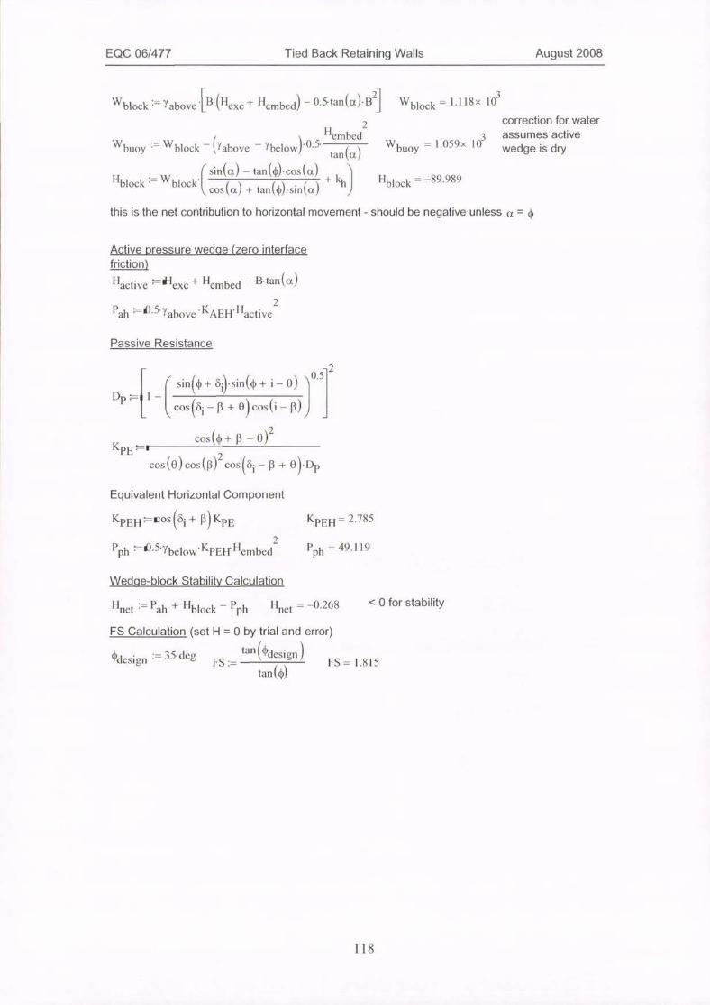
EQC 06/477 Tied Back Retaining Walls August 2008
Wblock = Yabove '_13·(H exe + Hembed) 0.5·tan (a)·B Wblock =
31.118x 10
Wbuoy
Hembed
Wblock - Yabove - Ybelow -RS tan(u)2
Wbuoy -
correction for water
3 assumes active1.059x 10
wedge is dry
Hblock=C sin(a) - tan(¢)·cos(a)
+k
Wblocklcos(a) + tan(4)·sin(01) hj Hblock = -89.989
this is the net contribution to horizontal movement - should be negative unless a = ¢
Active pressure wedqe (zero interface
friction)
- B·tan(u)Hactive -'Hexc + Hembed -
2
Pah -0-5.Yabove 'KAEH l|active
Passive Resistance
2
( sin(0 + Oil sin(* +i-0) Dp p, 1 -1 2
l cosltii -13 + 0 cos(i - 13)cos (0 + p- 0)2
KPE :-1
cos(0) cos (f!)2 cos61 -P+ 0·I)pEquivalent Horizontal Component
KpEI-1 -ros ji + pKPE KpEH= 2.785
2
Pph *8.5·7below KPEHHembed Pph = 49.119
Wedqe-block Stability Calculation
Hnet - Pah + '-'block - Pph Hnet - -0.268 < 0 for stability
FS Calculation (set H=Oby trial and error)
tan *design *design := 35-degFS := FS = 1.815
tan ¢
118
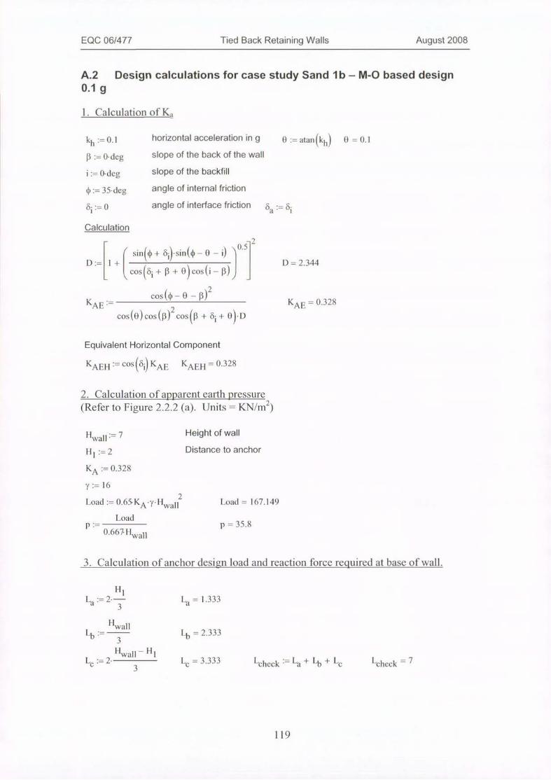
EQC 06/477 Tied Back Retaining Walls August 2008
A.2 Design calculations for case study Sand lb - M-O based design0.1 g
1. Calculation of Ka
kh:= 0.1 horizontal acceleration in g
B:= 0· deg slope of the back of the wall
i:= 0. deg slope of the backfill
0:= 35·deg angle of internal friction
Oi - angle of interface friction 6
:= atan k
1
hJ 0= 0.1
a
0
Calculation
r sin* + 6·sin((1) -O-i) 10.5 2D:= 1 + D = 2.344
Ccosc6i +B+ 8)cos 6 - B))
Kcos (0 -0- p)2
AE- K
cos(0)cos([fcos + di + o·DAE-
= 0.328
Equivalent Horizontal Component
KAEH :==cos i KAE KAEH = 0.328
2. Calculation of apparent earth pressure(Refer to Figure 2.2.2 (a). Units = KN/m2)
HwdF=7 Height of wall
H l:=2 Distance to anchor
KA := 0.328
7:=16
2
Load:=0.65·KA '7' HwallLoad = 167.149
P
Load
0.667 Elwall
p = 35.8
3. Calculation of anchor design load and reaction force required at base of wall.
HlLa:= 2.-3 La = 1.333
H
Lc := 2
wall
3
Hwall - H
3
Lb = 2.333
1
4 = 3.333 Lcheck := La + Lb +4 1 check -7
119
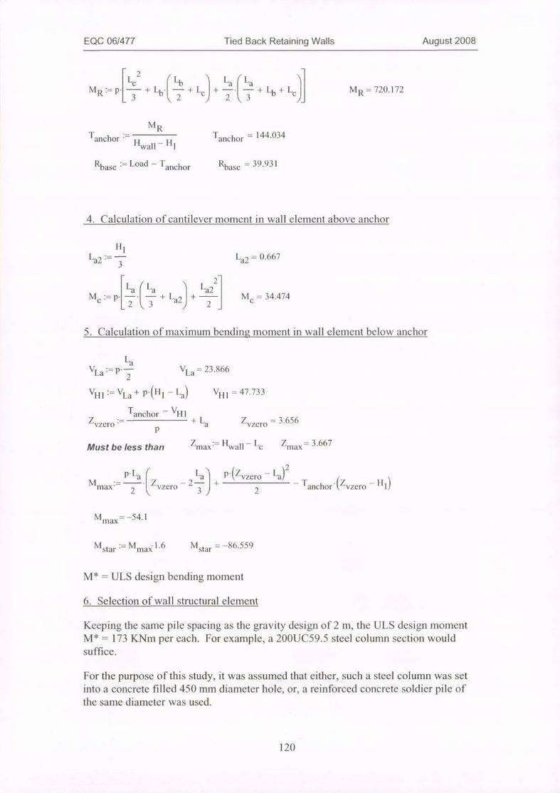
EQC 06/477 Tied Back Retaining Walls August 2008
M
LeR k P
3
2
- + Lb.C/ Lb-+L
2C
La r La+719+4 + Lc M R-= 720.172
MRTanchor - H Tanchor = 144.034wall - HI
Rbase := Load - 1 Rbase = 39.931anchor
4. Calculation of cantilever moment in wall element above anchor
La2 =
Ill3
112 = 0.667
2La r La h La2Mc:= p. -4 -+La21+ - Mc=34.474
2 (3 ) 1
5. Calculation of maximum bending moment in wall element below anchor
LaVLa - P2 VLa = 23.866
V„l:= VLa + P ' 11 - La VI-1 1 =47.733
Tanchor - VH 1Z
vzero ·- +La ZP
vzero= 3.656
Z ·=11wall - c
LMust be less than max' Zmax= 3.667
- 2- + P'(Zvzero
2
La,M
P.La r·= -·1 Z
max * 2 l vzero
12-T
anchor C Zvzero
-H 1J
Mmax- -54.1
M ·=Mmax ''6 Mstar = -86.559star
M* = ULS design bending moment
6. Selection of wall structural element
Keeping the same pile spacing as the gravity design of 2 iii, the ULS design momentM* = 173 KNm per each. For example, a 200UC59.5 steel column section wouldsuffice.
For the purpose of this study, it was assumed that either, such a steel column was setinto a concrete filled 450 mm diameter hole, or, a reinforced concrete soldier pile ofthe same diameter was used.
120

EQC 06/477 Tied Back Retaining Walls August 2008
7. Calculation of embedment depth for soldier piles
Simple Broms theory is used, with Kp calculated using Coulomb theory. Coulombtheory is used to be compatible with M-0 theory for later earthquake design case.
Interface friction is limited to */2 because Coulomb theory is unconservative at higherlevels of interface friction, the resulting value for Kp in this case is quite close to thevalue given by the NAVFAC charts which are based on log-spiral theory.
B := 0.45 Pile diameter
D:= 2.4 Depth of embedment of pile
y:= 8 Soil unit weight (buoyant)
0 := 35·deg
kh:= 0.1 horizontal acceleration in g 0 := atan(kh) 0 = 5.71 ldegp := 0· deg slope of the back of the wall
i:= 0. deg slope of the backfill
4 - atan(0.5-tan(0)) angle of interface friction (passive)
Passive Kp
< sin(0 + 4)·sin(0 + i-0) 0.5 2Dp:= 1-I Dp = 0.114Lcos(i -P+ O)cos(i - p)KPE.=
cos(* +B- 0)/K
COS (0)cos(11)2 cosi -0+ 0·DpPE -
7.387
Equivalent Horizontal Component
KPEH:=cos(bi + 11) KPE KpEH = 6.972
Ultimate Horizontal Resistance
H2
Ll
3
=-i-7-13-Kpii'r D HU
= 216.865
A strength reduction factor of 3 is recommended to be applied to the ultimatehorizontal resistance calculated using Broms' theory because of the large plasticstrains required to mobilise full passive resistance. Therefore, for piles spaced at 2 mcentres:
Design Resistance =217/3 = 72 KN each pile or 36 KN/m run
Design Demand (Rb84 = 36 KN/m
Therefore, embedment depth of 2.4 m is optimum.
121

EQC 06/477 Tied Back Retaining Walls August 2008
8. Check for internal stability
(True FS determined by successive reduction of 0)
H
f
d
7.447
l
t
a
4-Internal /
Stability ./
1/ ExternaStability
j
kh:= 0.1 horizontal acceleration in g 0 := atan (kh)13:=0·deg slope of the back of the wall
i:= 0·deg slope of the backfill
0:=29.Adeg angle of internal friction
4 := atan(0.5-tan(0)) angle of interface friction (passive) 6
0 = 5.71 ldeg
a:=0
Calculation
r sinA) + 6al ·sin -0-i) 0.52D:= 1+I 2 , 1 D= 2.098
leos(6+13 + 0) Costi -B)
Kcos(0 -O- 0)2
A E >
cos (o) cos([fcos[1 + 611K
+ 4·DAE= 0.403
Equivalent Horizontal Component
KAE|-1 = CON 2;a + B KAI. KAEH = 0.403
122
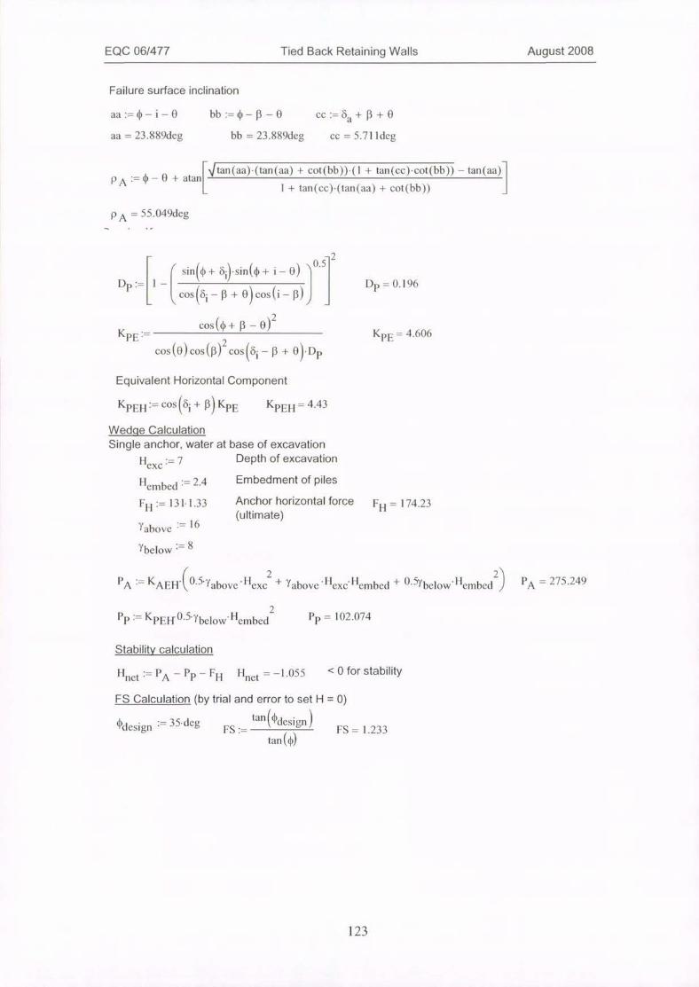
EQC 06/477 Tied Back Retaining Walls August 2008
Failure surface inclination
aa:=*-1-0 bb:=¢-0 -0 ec:= 68 + B + aa = 23.889deg bb = 23.88*leg cc = 5.711 deg
PA:= 0-0 + atan4tan(aa)-(tan(aa) + cot(bb))·(1 + tan(cc)·cot(bb)) - tat,(aa)
1 + tan(cc)·(tan(aa) + cot(bb))
PA= 55.049deg
2().5
r sin(* + 6,)-sin(0 + 1-0) jDp:= 1-1 Dp = ().196C cos<4 -B+0) cos(i - p)
KCOSI
PE >
cos(8)Cos(p
[0 + 0- 0)2KPE = 4.606
)2 cos@i - 13 + 0)·DpEquivalent Horizontal Component
KpEH:= cos 6i + 13) KPE KplEi-1 = 4.43
Wedqe Calculation
Single anchor, water at base of excavationDepth of excavationHexc:= 7
Hembed = 2.4 Embedment of piles
FH:=131·1.33
·= 16Yabove
Anchor horizontal force F
(ultimate)11 =
= 174.23
Ybelow := 8
2 21 PA = 275.249PA = KAEr 1 0.5 Yabove-Hexc + Yabove-'|exc. Hembed Hembed J+ 0.5Ybelow2
Pp := KpEHO-5.Ybelow Hembed Pp = 102.074
Stability calculation
'|net - PA - PP- FH Hnet - -1.055 < 0 for stability
FS Calculation (by trial and error to set H = 0)
4\Iesign := 35·deg FS:= FS = 1,233tan(¢designj
tan ((1)
123
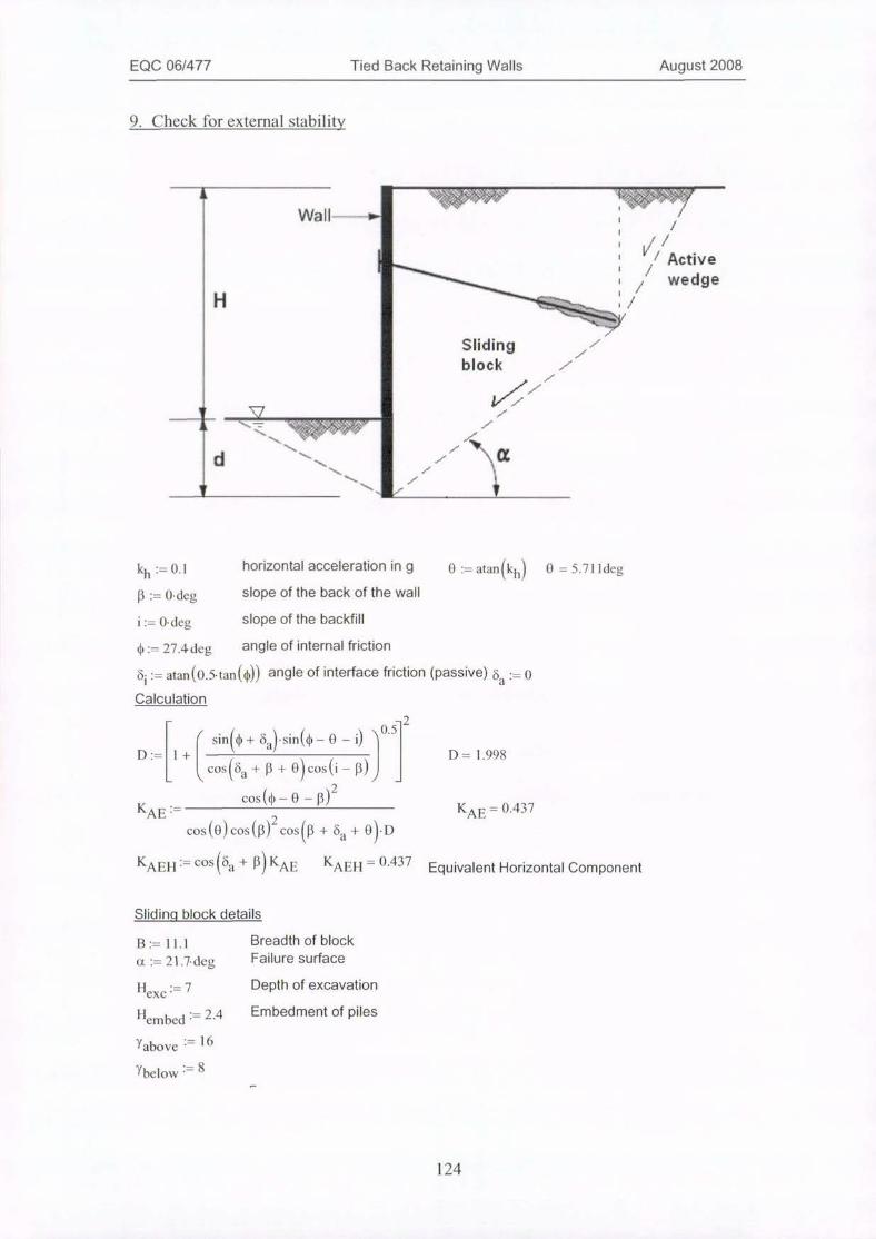
EQC 06/477 Tied Back Retaining Walls August 2008
9. Check for external stability
Wall---
H
I
d
Slidingblock
t
0 -= atan (k 0 = 5.71 ldeg
i
1 1V/
kh:= 0,1 horizontal acceleration in g
B := 0·deg slope of the back of the wall
i:= 0·deg slope of the backfill
1):= 27.4deg angle of internal friction
61 := atan(0.5·tan(@) angle of interface friction (passive) cia :. OCalculation
r sin(0 + *sin(0 -0-0 Y.52D:= 1+I i . 1 D= 1.998
cos(6a + #+ O)cosli -B)'2
KCoS (0-0-13)
AE -
cos(O)cos(13)2 cos13 + OaK
+ oj-DAE- ().437
KAEH= cosba + 11) KAE KAEH 0.437 Equivalent Horizontal Component
Sliding block details
B:= 11.1 Breadth of block
a:=21.7·deg Failure surface
| 'exe-7 Depth of excavation
||embed = 2.4 Embedment of piles
Fabove > 16
Ybelow - 8
124

EQC 06/477 Tied Back Retaining Walls August 2008
i , 21 3Wblock- Yabove B·(Hexc + Hembed - 0.5·tanla)·B J wblock = 1.277x 1(r
Wbuoy = *block - above - Ybelow5
Hembed
tan a
2
Wbuoy
correction for water
3 assumes active1.219 x 10
wedge is dry
< sin(a) - tan(0).cos(a)Hblock ·= Wblock' iC cosla) + tan*)·sina
+khj Hblock -
0.238
This is the net contribution to horizontal movement
Active pressure wedqe (zero interface
friction)
Hactive "-'exc + Hembed - B·tan(ot)2
' ah =O'5.yabove -KAEH Hactive
Passive Resistance
-2
f sin(0 + 6ij-sin(0 +i-0) 1Dp-,1-1
< cos Mi - 13 + 0 cos(i - 13)'2
COS (0 + P -0)KpE :- 1
cos (0)cos(13)2 cosi -11+ 0·DpEquivalent Horizontal Component
KPE]-1 -Eos <6i + 13 KpIE KPFH = 3.775
2
Pph NO.5·Ybelow'KPEII-"embed Pp, = 86.985
Wedqe-block Stability Calculation
Hnet := Pall + Hblock - Pph Hnet - -0.046 < 0 for stability
FS Calculation (set H=Oby trial and error)
tan *design ¢design = 35·deg FS := FS = 1.351
tan (4)
125
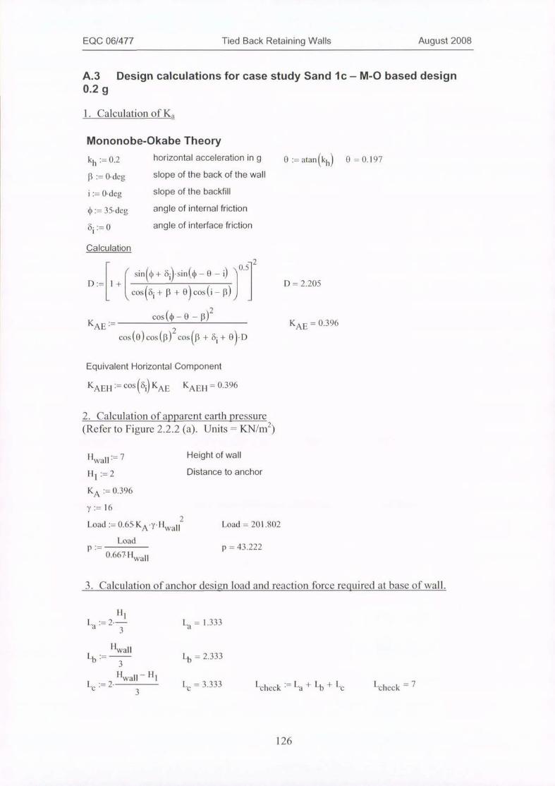
EQC 06/477 Tied Back Retaining Walls August 2008
A.3 Design calculations for case study Sand le - M-O based design0.2 g
1. Calculation of K,
Mononobe-Okabe Theory
kh:= 0,2 horizontal acceleration in g 0 := atan(kh) 0 - 0.19713 := 0·deg slope of the back of the wall
i:= 0. deg slope of the backfill
¢:= 35·dea angle of internal friction
angle of interface frictionOi
Calculation
r sin((f + 611*sin(0 -0-i) ju.5 2D-= 1+I ' ' . I D= 2.205
L cos(i+P+0) coS(i - p)j
cos (0 -0- p)2KAE KAE = 0.396
cos(0)cos (P)2 cos P + tii + 0)· D
Equivalent Horizontal Component
KACH = cos6i KAE KAEH = ()-396
2. Calculation of apparent earth pressure
(Refer to Figure 2.2.2 (a). Units = KN/m2)
Hwall:=7 Height of wall
H l:= 2 Distance to anchor
KA := 0.396
7:= 16
2
Load:= 0.65·KAY- 11wallLoad = 201.802
Loadp := p = 43.222
().667 Hwall
3. Calculation of anchor design load and reaction force required at base of wall.
La
H
-2.-3
La
= 1.333
H
4:== -
LC := 2
wall
3
Lan - H
3
Lb = 2.333
Le = 3.333 Lcheck - L2+4+ I C check -7
126
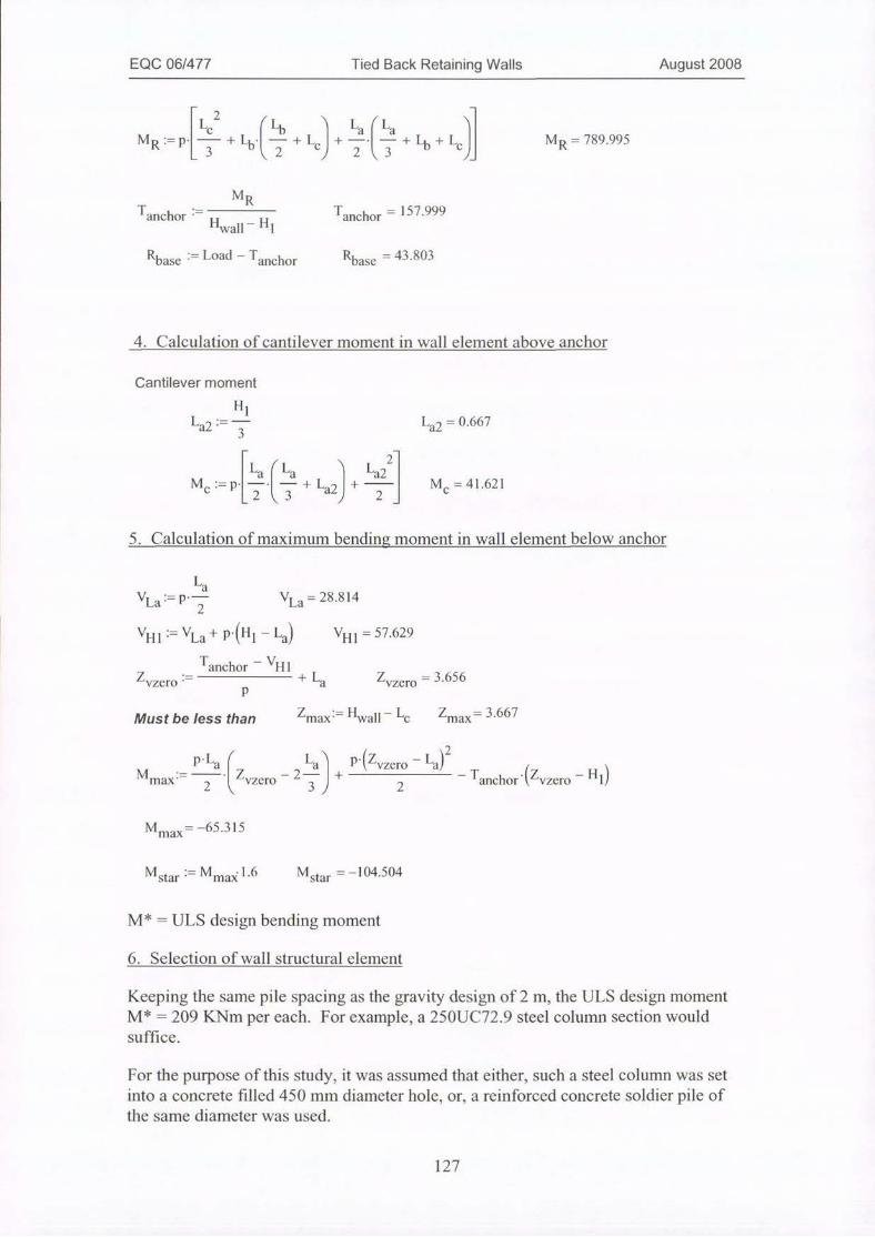
EQC 06/477 Tied Back Retaining Walls August 2008
M4
2
c Lb2
L CL
+ It) + 919 +4+4J MR= 789.995
MRTanchor Tanchor = 157.999
Hwall- Hl
Rbase = Load - Tanchor Rbase = 43.803
4. Calculation of cantilever moment in wall element above anchor
Cantilever moment
H1La2:== 3- La2 = 0.667
M La LaC :=P.--1 -2 43
1 L
+La2j + -
2
a2M
2C
= 41.621
5. Calculation of maximum bending moment in wall element below anchor
LaVLa P * -3- VLa -28.814
411 -VLa+P*(111 - La) VH1 = 57.629
Z
T
vzero
anchor - VH 1+L
Pa
Zvzero
= 3.656
Z H L Zmax= 3.667Must be less than max -- wall- c
M -2 -9-) + P.(zvzero
2
- La/max '
.La r= -liz
2 4vzero
)2-T
anchor (Zvzero
-H 1J
Minax- -65.315
M ·= Mma*1.6 M star --104.504star '
M* = ULS design bending moment
6. Selection ofwall structural element
Keeping the same pile spacing as the gravity design of 2 m, the ULS design momentM* = 209 KNm per each. For example, a 250UC72.9 steel column section wouldsuffice.
For the purpose of this study, it was assumed that either, such a steel column was setinto a concrete filled 450 mm diameter hole, or, a reinforced concrete soldier pile ofthe same diameter was used.
127
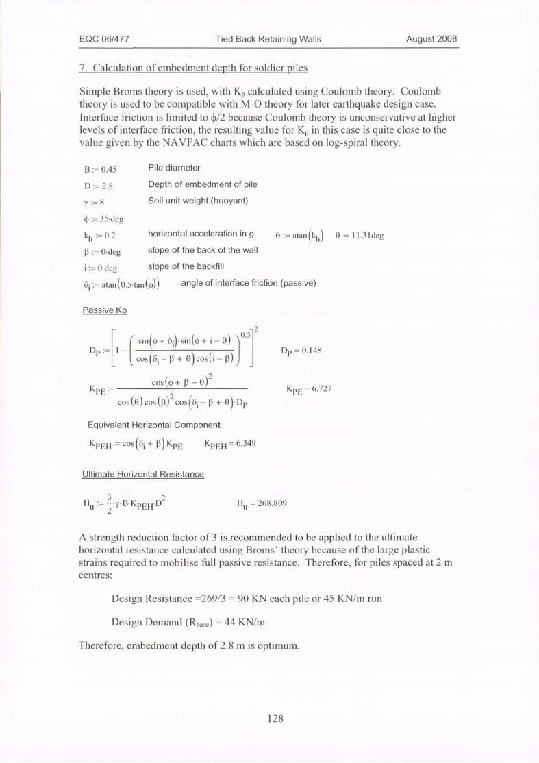
EQC 06/477 Tied Back Retaining Walls August 2008
7. Calculation of embedment depth for soldier piles
Simple Broms theory is used, with Kp calculated using Coulomb theory. Coulombtheory is used to be compatible with M-0 theory for later earthquake design case.
Interface friction is limited to ¢/2 because Coulomb theory is unconservative at higherlevels of interface friction, the resulting value for Kp in this case is quite close to thevalue given by the NAVFAC charts which are based on log-spiral theory.
B := ().45 Pile diameter
D:= 2.8 Depth of embedment of pile
7:= 8 Soil unit weight (buoyant)
¢ := 35· deg
kh:= 0.2 horizontal acceleration in g 0 :=atan (kh)13 := 0· deg slope of the back of the wall
i:= 0. deg slope of the backfill
4 = atan(0.5·tan(*)) angle of interface friction (passive)
0 = 11.3 ldeg
Passive Kp
20.5
< sin(0 + bi) sin(0 +i-O) jDp:== 1- Dp = 0.148C cos(4-0 +0 cos(i -p)
COSCKim:=
CoS (0) Cos(p]
0+13-
2 t
I cos(6
,2
8,
1-13 + 0)·DK
P
PE-6.727
Equivalent Horizontal Component
Kp[:1':= cos 6i + 13) KPE KPEH = 6.349
Ultimate Horizontal Resistance
113
U.- 2··y·B·KPEH D2
11U
= 268.809
A strength reduction factor of 3 is recommended to be applied to the ultimate
horizontal resistance calculated using Broms' theory because ofthe large plasticstrains required to mobilise full passive resistance. Therefore, for piles spaced at 2 mcentres:
Design Resistance =269/3 = 90 KN each pile or 45 KN/m run
Design Demand (Rbage)=44 KN/m
Therefore, embedment depth of 2.8 m is optimum.
128
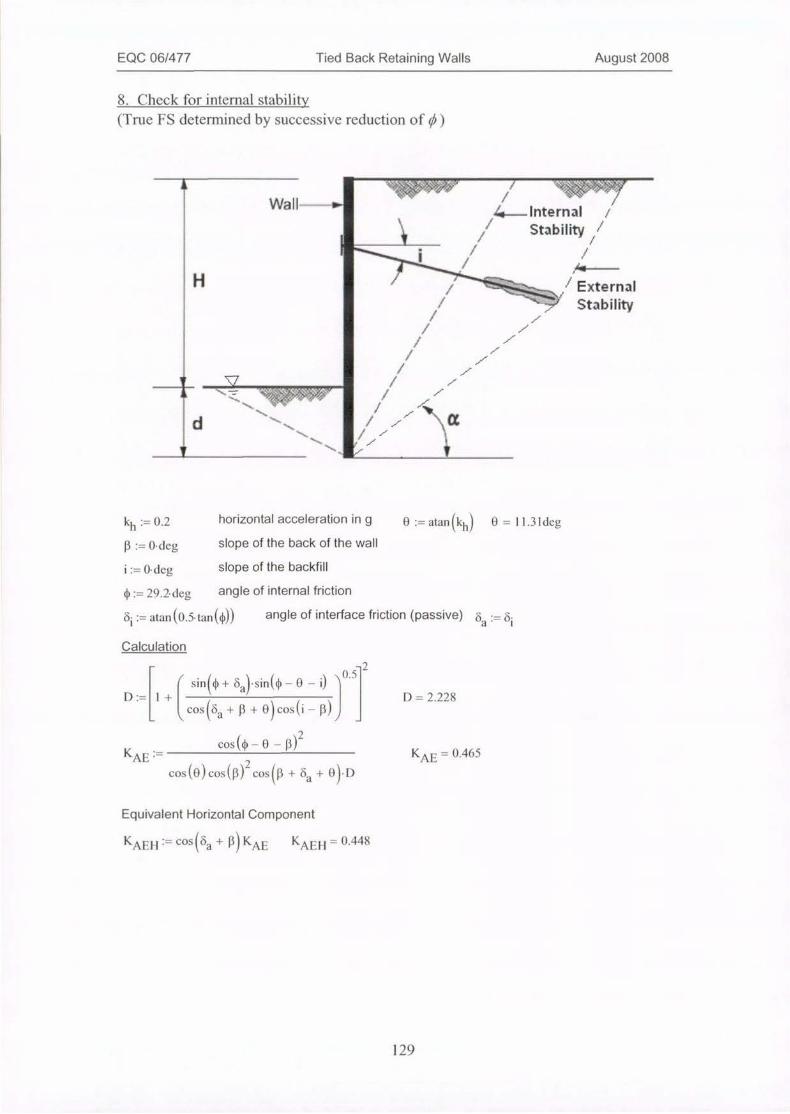
EQC 06/477 Tied Back Retaining Walls August 2008
8. Check for internal stability
(True FS determined by successive reduction of 0 j
A
H
I U
f
d \/
4.Internal
Stability
j
'4--
€624>- / External7 Stability
1
kh:= 0.2 horizontal acceleration in g 8 := atan (kh)B:= 0· deg slope of the back of the wall
i:=0·deg slope of the backfill
¢ := 29.2- deg angle of internal friction
4 = atan (0.5· tan(*)) angle of interface friction (passive) 6
0=
a = 6
11.3ldeg
Calculation
2().5
< sill(* + tia sin((1) -0-J D:= 1+1 D = 2.228
cos(tia +13+ 8)cos(i - 11)cos (0 -0- p)2
KAE = 0.465KAE *cos(0) cos (B)Lcosp + 6a + 0 D
Equivalent Horizontal Component
KA'·H:==cos{6a + KAE K/\111= 0.448
129
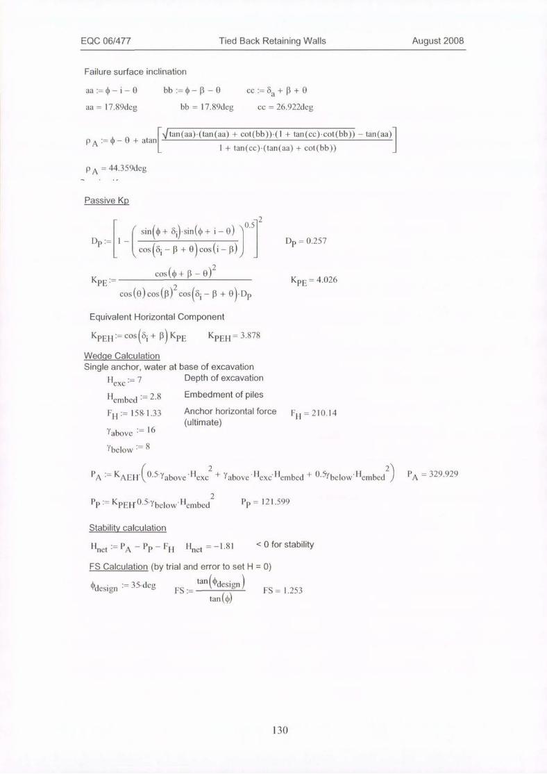
EQC 06/477 Tied Back Retaining Walls August 2008
Failure surface inclination
aa:-0-i-0 bb:=4)-P-0 ec:=6a +B+aa = 17.89deg bb = 17.89deg cc = 26.922deg
PA -0 -0 + atan+an(aa)-(tan(aa) + cot(bb)HI + tan(cc)·cot(bb)) - tan(aa)-1
1 + tan(ce)·(tan(aa) + cot(bb)) J
PA = 44.359deg
Passive Kp
-2
< sin((1) + bi)-sin(0 +i- 0) *5Dp = ().2571,P--1 -cosi-13+0)cos(i- 13)3
cos(0 +P- 0)2KPE:=
cos (0) cos (p)2 cos tii -13+ 0·DK
P
PE -4.()26
Equivalent Horizontal Component
KpEN:= cos 6, + 13KPE KpEH = 3.878
Wedqe Calculation
Single anchor, water at base of excavation
Hexc 7 Depth of excavation
I lembed = 2.8 Embedment of piles
FH:= 158-1.33 Anchor horizontal force F
(ultimate)Yabove := 1 6
11 ==210.14
l'below > 8
2 21
PA r= KAEH Hexc + Yabove *Hexc Hembed + O57below Hembed PA = 329.9290.5· Y above 2
IP:= KPEN . Hembed Pp = 121.5990.5·Ybelow
Stability calculation
"net -=PA - PP - Fll Hnet -1.81 < 0 for stability
FS Calculation (by trial and error to set H = 0)
design .= 35·deg FS := FS = 1.253tandesignj
tan (*)
130
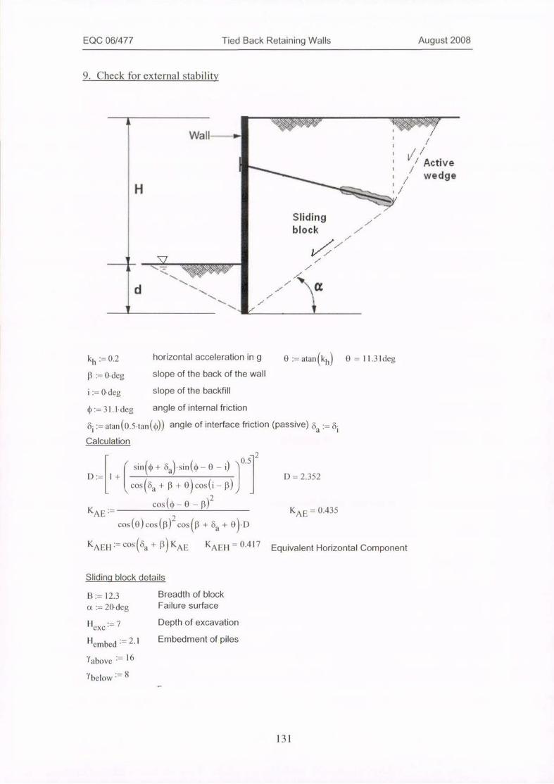
EQC 06/477 Tied Back Retaining Walls August 2008
9. Check for external stability
A
Wall--
H
Slidingblock
U t
f
d
j
7
f
1 0= 11.3 ldeg
0.435
kh:= 0,2 horizontal acceleration in g 0:= atan (k
p:= 0· deg slope of the back of the wall
i:= 0-deg slope of the backfill
4):=31.1.deg angle of internal friction
6i := atan(0,5-tan(¢)) angle of interface friction (passive) 621 :Calculation
r sin + cia) sin<¢ -0-i 0.5
D:= 1+I D = 2.352
< cOS(6,1 Cosli - [3)2
COS (0 -0-P)1<AE :- - KAE =
COS(0)COS([3)Zeos B + 88 + 0)·D
KAEH = costia + p) KAE KAEH = O.417 Equivalent Horizontal Component
Sliding block details
B:= 12.3 Breadth of block
u := 20 deg Failure surface
"exe · 7 Depth of excavation
Hembed = 2.1 Embedment of piles
yabove := 16
Ybelow > 8
131
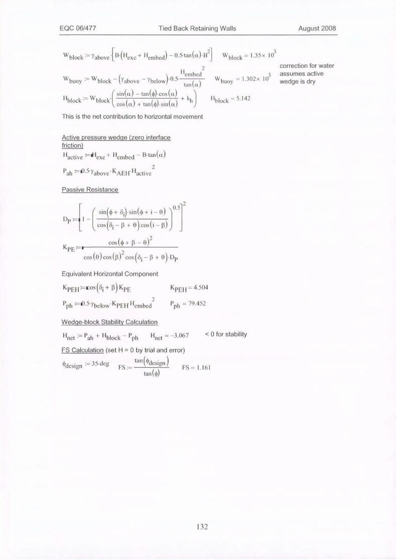
EQC 06/477 Tied Back Retaining Walls August 2008
*'block := Yabove'l-B.(11exe
3+ Hembed - 0·5·tan(a)·B Whlock = 1.35 x 10
Wbuoy
Hembed
Wblock - Tabove - Ybelow) 05 tan (a
2
Wbuoy =
correction for water
3 assumes active1.302 x 1(r
wedge is dry
C sin(a) - tan(¢)·cos(a)Elblock :=Wblockl cos(a + tan(*)·sin(ot)
+kh
Hblock
=5.142
This is the net contribution to horizontal movement
Active pressure wedqe (zero interface
friction)
"active *"exe + Hembed - B·tan((]t)2
Lh ;=i).5.yabove KAE] 1*"active
Passive Resistance
r sin(4) + 61)-sin(0 + i- 0) 0.5 2Dp=.1-I ;(cos (4 - p + O) cos(i - 11)
cos (0 +B- 0)2KPE -1
cos(0)cos (p)Lcos<ji - 13 + 0-Dp
Equivalent Horizontal Component
KpEHZ=Cos i + 13KI'E KPEH = 4.5()4
2
ph 7=O.5-Ybelow KPEIFHembed P. = 79.452
Wedqe-block Stability Calculation
I Inet = Pah + Hblock - Pph ||net = -3.067 < 0 for stability
FS Calculation (set H=Oby trial and error)
¢ilesign = 35·deg FS :=tan *design
FS= 1.161
tanct)
132
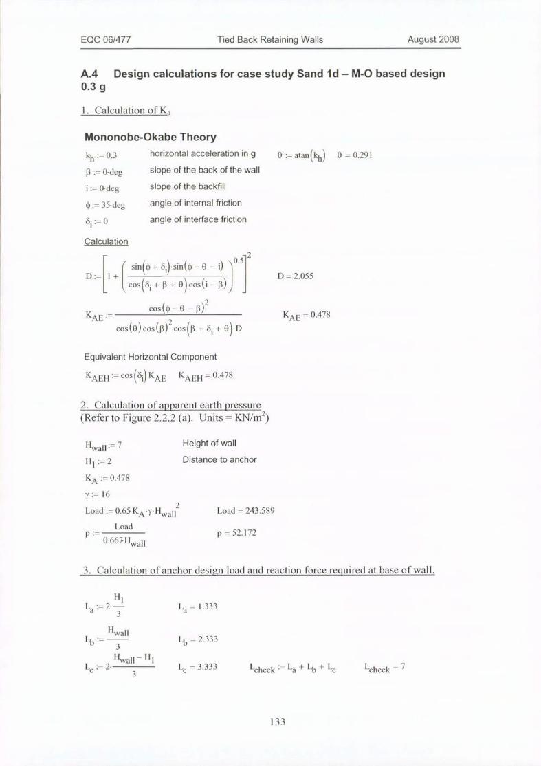
EQC 06/477 Tied Back Retaining Walls August 2008
A.4 Design calculations for case study Sand ld - M-O based design0.3 g
1. Calculation of K
Mononobe-Okabe Theory
kh:= 0.3 horizontal acceleration in g 0 := atan (kh) 0 = 0.291
B := 0·deg slope of the back of the wall
i:= 0·deg slope of the backfill
0 := 35·deg angle of internal friction
4-0 angle of interface friction
Calculation
r sin(* + bil·sin(0 -0-i) 0.5 2D:= 1+I ' ' I D= 2.055
leos (61 + P + 8) COS (i - p) j
cos (0 -0- p)2KAE KAE = 0.478
f ' / \Z / 1
cosle) cos<[3) cos(13 + bi + 0) D
Equivalent Horizontal Component
- 0.478KAEH = cOs KAE KAEH
2. Calculation of apparent earth pressure
(Refer to Figure 2.2.2 (a). Units = KN/m2)
HwaH:== 7 Height of wall
HI := 2 Distance to anchor
KA := 0.478
7:= 16
Load := 0.65·KA'Y "wall- Load = 243.589
LoadP:= p = 52.172
().667·Hwall
3. Calculation of anchor design load and reaction force required at base of wall.
111La := 2.-3- La = 1,333
1
H
1
wall
3
Hwall - H
3
1-b :
1='C
= 2.333
=3.333 1 check --L
a 'b+L 1
C theck -7
133

EQC 06/477 Tied Back Retaining Walls August 2008
M4
R:== P. 3
2
- + Lb.</ Lb2
L CL
+ Le] + 9-·lf +4+LCJ MR-= 953.579
MRTanchor := Tanchor = 190.716
Hwall - 1-'l
Rbase = Load - Tanchor Rbase = 52.873
4. Calculation of cantilever moment in wall element above anchor
La2 >
H
3
1
La2 = 0.667
M La (La 1 Lc:= p_27 + La2J + -
2
a2M
2C
= 50.239
5. Calculation of maximum bending moment in wall element below anchor
LaVLa :- P2 VLa = 34.781
411:= VLa + P-(Hl - La VH 1 = 69.562
Z
T
vzero '
anchor - VIi 1+ La Z
Pvzero
= 3.656
Must be less than Zmax = Hwall- cL Zmax= 3.667
MP.La <
max 2 vzero 2 -9-) + P.{Z-L
vzero a
2
)2-Tanchor (Z
vzero-H 1J
Mmax= -78.84
M ·=Mmail.6 Mstar --126.144star -
M* = ULS design bending moment
6. Selection ofwall structural element
Keeping the same pile spacing as the gravity design of 2 m, the ULS design moment
M* = 252 KNm per each. For example, a 250UC72.9 steel column section wouldsuffice.
For the purpose of this study, it was assumed that either, such a steel column was set
into a concrete filled 450 mm diameter hole, or, a reinforced concrete soldier pile ofthe same diameter was used.
134
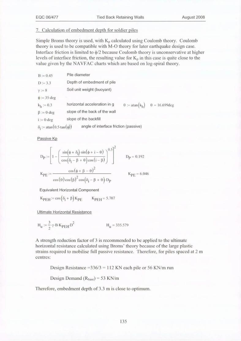
EQC 06/477 Tied Back Retaining Walls August 2008
7. Calculation of embedment depth for soldier piles
Simple Broms theory is used, with Kp calculated using Coulomb theory. Coulombtheory is used to be compatible with M-0 theory for later earthquake design case.
Interface friction is limited to */2 because Coulomb theory is unconservative at higherlevels of interface friction, the resulting value for Kp in this case is quite close to thevalue given by the NAVFAC charts which are based on log-spiral theory.
B := 0.45 Pile diameter
D:= 3.3 Depth of embedment of pile
7:=8 Soil unit weight (buoyant)
0 :=35·deg
kh:= 0.3 horizontal acceleration in g 0:= atan (kB := 0· deg slope of the back of the wall
i:= 0. deg slope of the backfill
4 := atan(0.5·tan(0)) angle of interface friction (passive)
hj 0 -16.699deg
Passive Kp
< sin(* + bi)-sin((1) +i-0) 0.5 2Dp:= 1 -1 Dp = 0.192C coscoi - p + 0)cos(i - p)3
cos(*+P- 8)2KpE:=
cos(0)cos(p)2 cosi -P+ 0·DKpIE = 6.046
P
Equivalent Horizontal Component
KPE'-1 := cos bi + P KPE KpEH = 5.7()7
Ultimate Horizontal Resistance
11u 7. B·KPEH U= 335.579
A strength reduction factor of 3 is recommended to be applied to the ultimate
horizontal resistance calculated using Broms' theory because ofthe large plastic
strains required to mobilise full passive resistance. Therefore, for piles spaced at 2 mcentres:
Design Resistance =336/3 = 112 KN each pile or 56 KN/m run
Design Demand (Rbase) = 53 KN/m
Therefore, embedment depth of 3.3 m is close to optimum.
135
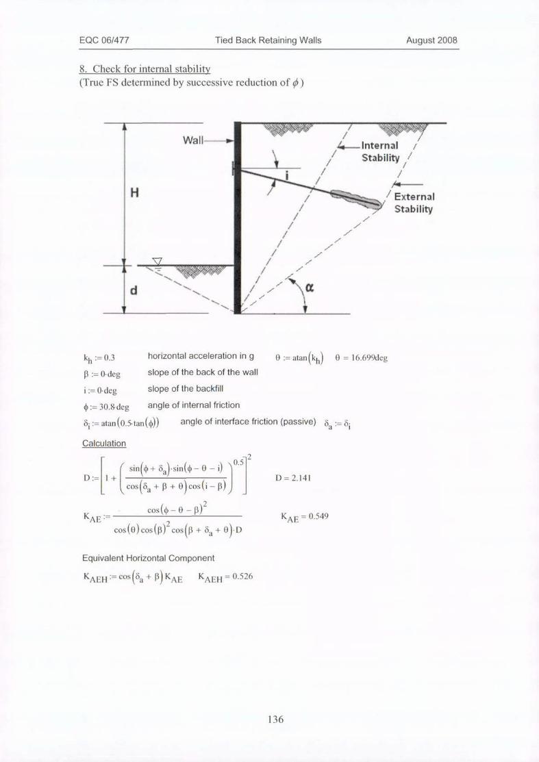
EQC 06/477 Tied Back Retaining Walls August 2008
8. Check for internal stability
(True FS determined by successive reduction of 0)
A
H
I U
d
t
4-Internal /
Stability /1
--/ External3 Stability
f
kh:= 0.3 horizontal acceleration in g 0 := atan (kp:= 0. deg slope of the back of the wall
i:= 0. deg slope of the backfill
¢ := 30.*deg angle of internal friction
4 := atan(0.5·tan(0)) angle of interface friction (passive)
hJ 0 =
a= 25
16.699deg
1
Calculation
< sinf¢ + 6.'sin(0 -0-i) 7-5 2D:= 1+I D=2.141
C couda + 13 + 0)cos(i - 13) 3cos (0 -0- p)2
KAET- KAE = 0-549cos(0)cos(p)2 cos 0+ %+G-D
Equivalent Horizontal Component
KAEH =cos a + 13 KAI€ KAEH = O-526
136
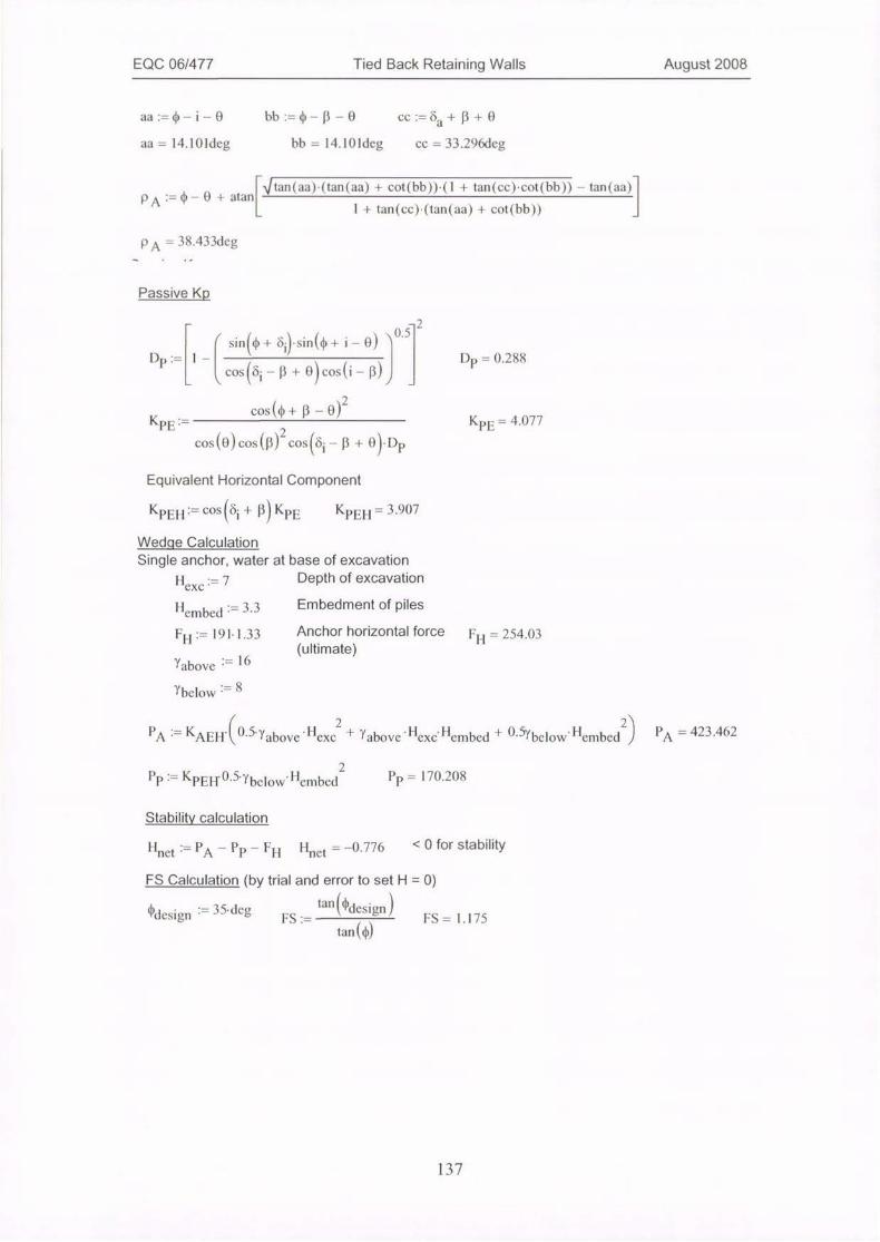
EQC 06/477 Tied Back Retaining Walls August 2008
aa:=0-i-0 bb:=4)-p-0 ec:= 63+ P+0
aa = 14.10ldeg bb = 14.10Meg cc = 33.296deg
PA = 0- 0 + atan+an(aa)·(tan(aa) + cot(bb))·(1 + tan(cc)·cot(bb)) - tan(aa)-1
1 + tan(cc)·(tan(aa) + cot(bb))
PA= 38.433deg
Passive Kp
r sin(* + 6i)·sin(* +i- 0) 0.5 2I)P:= 1 -1 ,
F
Dp= 0.288l cos (bi- 11 + O) cos(i- 11)
KpEcos(0 + 13 - 0)2
cos(0) cos(13)2 cosdi -P+ 0·DK
P
PE=4.()77
Equivalent Horizontal Component
KpE]-1:=costii-+ P)KPE KPE' 1 =3.907
Wedqe Calculation
Single anchor, water at base of excavation
1-'exc:-7 Depth of excavation
i lembed = 3.3 Embedment of piles
11 1 := 191- 1.33
Yabove := 16
Anchor horizontal force i
(ultimate)11 == 254.()3
Ybelow := 8
PA = KAE[1(C·5.'fabove 'exc + Yabove Hexclienibed + Chtbelowl-lembed2 PA = 423.462
2 pp = 170.208PP := KPE"-O.5.ybelow*'lembed
Stability calculation
"net - PA - PP - Fll linet - -0-776 < 0 for stability
FS Calculation (by trial and error to set H = 0)
*design := 35·deg FS:= FS= 1,175tan<*design
tan(¢
137
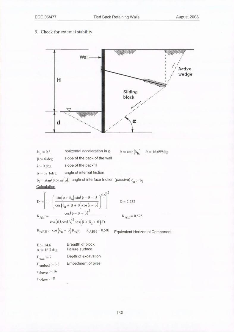
EQC 06/477 Tied Back Retaining Walls August 2008
9. Check for external stability
AtN
H
U
d
Slidingblock
f
@DI#
/ f1 fl
Vt Active
l wedge
-7
j
jt
1 1V/
kh:= 0.3 horizontal acceleration in g 0 := atan (kh) 0 = 16.699deg13 := 0·deg slope of the back of the wall
i:= 0- deg slope of the backfill
0 := 32.1·deg angle of internal friction
4 - atan(0.5·tan(@) angle of interface friction (passive) ba := ACalculation
-2. 0.5
< sin + basin(0 -0-0 1D:= 1+I . 1 D = 2.232
l cos(cia + 13 + 0 jcosli -p)cos ((1)-0 - p)2
KAE KAE = 0.525
cos(0)cos([3)ZcosB + tia + 8 D
KAEH = cosa + 13 KAE KAE}1 - 0501 Equivalent Horizontal Component
B:= 14.6 Breadth of block
a := 16.7-deg Failure surface
"exc= 7 Depth of excavation
Hembed - 3.3 Embedment of piles
Yabove 16
Ybelow = 8
138

EQC 06/477 Tied Back Retaining Walls August 2008
i , 21Wblock :=yat)ove B·(Hexc + Hembed- 0.5·tanla)·B -1 Wblock = 1-894>< 103
Wbuoy
2
HembedW:= Wblock - fabove - Ybelow)-C5 tan <a buoy
correction for water
3 assumes active1.749x 10-
wedge is dry
11block =r sinla) - tan(0)·cos(a)
WblocklC cosa + tan*·sina
+khj Hblock = 46.517
This is the net contribution to horizontal movement
Active pressure wedqe (zero interface
friction)
Hactive "'Hexc + Hembed - B·tan(ox)2
Pah *85 Yabove-KAEH Hactive
Passive Resistance
-2
< sin(* + bil·sin(0 +i-0) j05Dp =11 -1
l co*i -P+ 0) cos (i -p)cos (0 + p- 0)2
KpE h-1
cos(0)cos (13)2 cos@i -0 + 0)·DpEquivalent Horizontal Component
KpEH -Cos6i + [3KPE KpEH= 4.367
P . = 190.211Pph ;=8.5·ybelow'KPENHembed pn
Wedqe-block Stability Calculation
Hnet := Pah + Hblock - Pph Hnet =-3.21 < 0 for stability
FS Calculation (set H=Oby trial and error)
design := 35· deg FS:=tan design
FS= 1.116
tan ((1)
139
EQC 06/477 Tied Back Retaining Walls August 2008
A.5 Design calculations for case study Sand le - M-O based design0.4 g
1. Calculation of Kit
Mononobe-Okabe Theory
41 := 0,4 horizontal acceleration in g 0 := atan (kh) 0 = 0.3811.3:= 0· deg slope of the back of the wall
i:=0·deg slope of the backfill
$:= 35·deg angle of internal friction
di:= 0 angle of interface friction 6 -= 6a - i
Calculation
2
( sin((I) + 6ij·sin((I) -0-i) Y5D:-1+I ' ' I D= 1.892
l co*i +P+0) cos (i - 13)j
KAE r=cos(0 -O- p)2
K
cos (0)cos(pfcosp + tii + 0·DAE=
0.581
2. Calculation of apparent earth pressure(Refer to Figure 2.2.2 (a). Units = KN/m2)
1-1 Height of wallwall:= 7
H 1 := 2 Distance to anchor
KA := 0.581
y:= 16
2
load:=0.65·KAY'HwallLoad = 296.078
Load
P:= p = 63.4130.667·H
wall
3. Calculation of anchor design load and reaction force required at base of wall.
Moments about base
H1La:= 2.7 La - 1.333
HwallLb:
LC :
3
Hwall-
3
H
Lb = 2.333
4 = 3.333 Lcheck := a + 0L L +4 Lcheck = 7
140
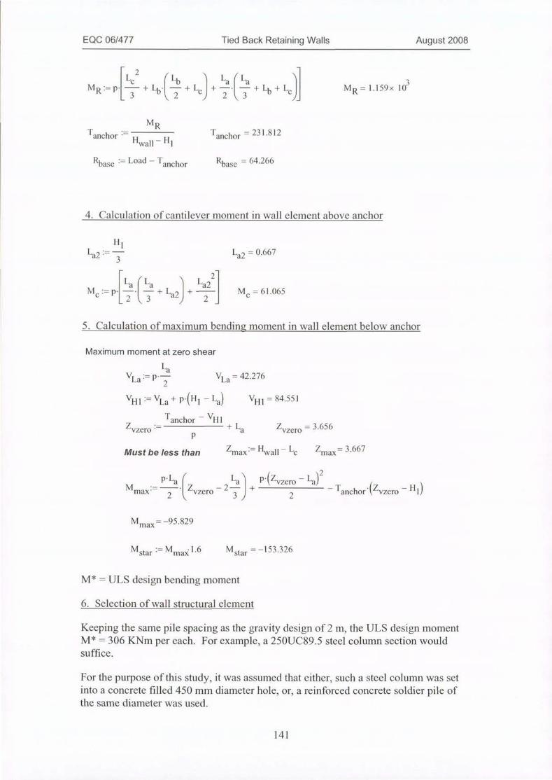
EQC 06/477 Tied Back Retaining Walls August 2008
2
LCMR I- P -3 + L.b-2+ Lc + -3-3 + Lb + 1,c MR= 1.159x 1032 43
MRTanchor - " H Tanchor =231.812
1-lwall - 1
Rbase = Load - Tanchor Rbase = 64.266
4. Calculation of cantilever moment in wall element above anchor
42
H
3
1La2 -
0.667
M La Lac:= p.-3-'ll-
La22+ La2.J + M
2C
= 61.065
5. Calculation of maximum bending moment in wall element below anchor
Maximum moment at zero shear
LaVia:= p. T VLa = 42.276
VH 1 - VLa + P-(Hl - La) VHI = 84.551
Z
T
vzero
anchor - VH 1+L
Pa
Zvzero
= 3.656
Must be less thanZ
max '=H
wail Le Zniax= 3.667
M.La r
niax* 2 vzero - 2-La) + P'(Zvzero - La)
2 - Tnchor CZvzero
-H 1J
Mmax= -95.829
M star - Mmax 1.6 Mstar =-153.326
M* = ULS design bending moment
6. Selection of wall structural element
Keeping the same pile spacing as the gravity design of 2 m, the ULS design momentM* = 306 KNm per each. For example, a 250UC89.5 steel column section wouldsuffice.
For the purpose of this study, it was assumed that either, such a steel column was setinto a concrete filled 450 mm diameter hole, or, a reinforced concrete soldier pile ofthe same diameter was used.
141

EQC 06/477 Tied Back Retaining Walls August 2008
7. Calculation of embedment depth for soldier piles
Simple Broms theory is used, with Kp calculated using Coulomb theory. Coulombtheory is used to be compatible with M-0 theory for later earthquake design case.
Interface friction is limited to ¢/2 because Coulomb theory is unconservative at higherlevels of interface friction, the resulting value for Kp in this case is quite close to thevalue given by the NAVFAC charts which are based on log-spiral theory.
B := 0.45 Pile diameter
D:= 3.8 Depth of embedment of pile
y:=8 Soil unit weight (buoyant)
0 := 35·deg
kh:= 0,4 horizontal acceleration in g 0 := atan (kh)p := 0·deg slope of the back of the wall
i:= 0. deg slope of the backfill
4 := atan(0.5·tan(*)) angle of interface friction (passive)
0 = 21.80ldeg
Passive Kp
< sin(0 + 4)·sin(0 +i-0) 0.5 2DP:= 1 -1 Dp= 0.254£ cos Ctii -B + 0) cos (i -13) J
KPE:=COS (0 + 0 -
'2 1
cos(0)cos(p) cos<6
0)2
i -11 + 0)-DK
P
PE -5333
Equivalent Horizontal Component
KpEH-cos 6i + 13 KpE KpH - 5.034
Ultimate Horizontal Resistance
113
li *-2
2
7.B·KPE.11- D H U= 392.514
A strength reduction factor of 3 is recommended to be applied to the ultimate
horizontal resistance calculated using Broms' theory because of the large plasticstrains required to mobilise full passive resistance. Therefore, for piles spaced at 2 incentres:
Design Resistance =392/3 = 130 KN each pile or 65 KN/m run
Design Demand (Rbaqe) = 64 KN/m
Therefore, embedment depth of 3.8 m is close to optimum.
142
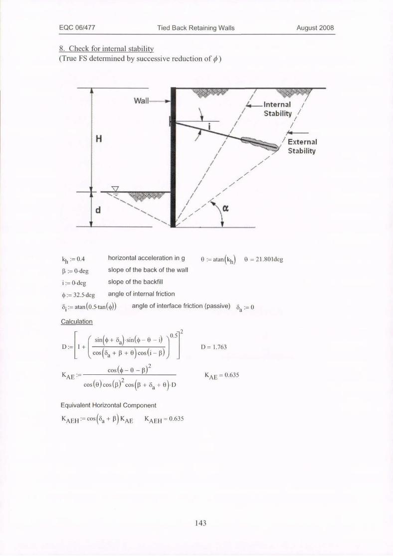
EQC 06/477 Tied Back Retaining Walls August 2008
8. Check for internal stabilitv
(True FS determined by successive reduction of 0)
Wall-4.---Internal
Stability
i
H
i
!
' External
0 Stability
kh:= 0.4 horizontal acceleration in g 0 :=atan(kh) 0 = 21.80ldeg13 := 0·deg slope of the back of the wall
i:= 0. deg slope of the backfill
0:= 32.5deg angle of internal friction
Oi := atan(0.5·tan(*)) angle of interface friction (passive) 6, 2- '
Calculation
r sin@ + ba'sin(0 - 0 - 1)D:= 1+I D = 1.763
leos(oa + p + ejeosti- B)
KAE =cos(* -O- p)2
K
cos (0)cos(p)2 cos@ + 68 + 0)AE 0.635
Equivalent Horizontal Component
KAEH - cos fa + 13 KAE KAEH - 0.635
t
tt
d
143
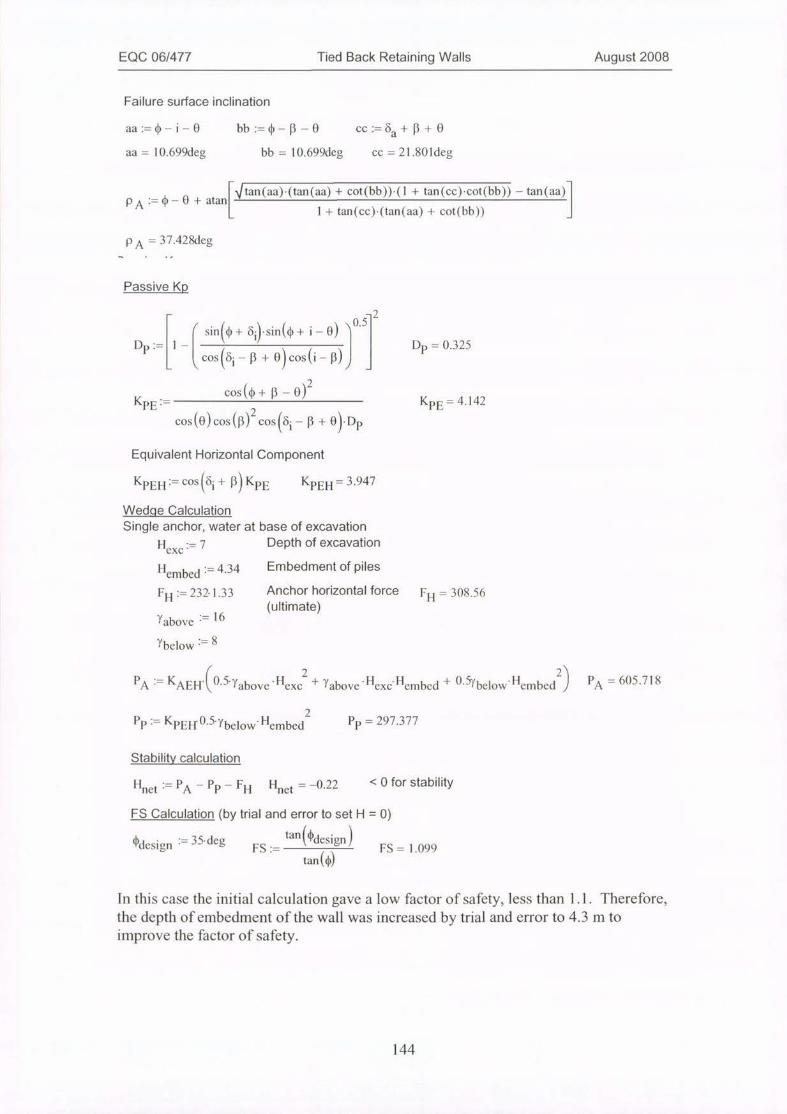
EQC 06/477 Tied Back Retaining Walls August 2008
Failure surface inclination
aa:=*-i- 0 bb:= 0-11-0 ce:= Oa + B + 0aa = 10.699deg bb = 10.699deg cc = 21.80ldeg
PA -0-0 + atan tan (aa)·(tan (aa) + cot(bb))·(1 + tan (cc)·cot(bb)) - tan (aa)11 + tan(cc)·(tan(aa) + cot(bb)) J
PA= 37.428deg
Passive Kp
-2
r sinC¢ + 61)·sin(0 + 1-0) 0-5Dp:= 1 - Dp = ().325Ccostii -P+ 0)cos(i - 11))
cos(0 +13- 0)2KPE:=
cos(0) cos ('fcos- P + 0·DKPE = 4.142
P
Equivalent Horizontal Component
KpEH:= cos bi + 13 KPE KPEH = 3.947
Wedqe Calculation
Single anchor, water at base of excavation
Hexc = 7 Depth of excavation
Hembed := 4.34 Embedment of piles
FH := 232-1.33
Yabove := 16
Anchor horizontal force F
(ultimate)H
= 308.56
ybelow - 8
PA -= KAEH'7above
Pp:= KPEHO-5.ybelow H
Stability calculation
·11 2exe
2
embed
+ Yabove ·Hexc Hembed + 0.57 below H
Pp = 297.377
embed2 PA-
= 605.718
'Inet :- PA - PP - FH Hnet = -0.22 < 0 for stability
FS Calculation (by trial and error to set H = 0)
*design = 35·deg FS := tan*design FS = 1.099
tan (0
In this case the initial calculation gave a low factor of safety, less than 1.1. Therefore,the depth of embedment of the wall was increased by trial and error to 4.3 m to
improve the factor of safety.
144
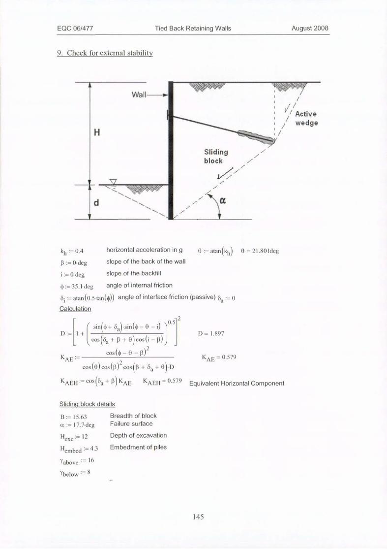
EQC 06/477 Tied Back Retaining Walls August 2008
9. Check for external stabilitv
A
L,/' Active, 1 wedge
H
Slidingblock
1 1V/
I
d
kh:= 0.4 horizontal acceleration in g 0 := atan(kh) 0 = 21.80ldeg13:= 0· deg slope of the back of the wall
i:= 0. deg slope of the backfill
¢ :=35.1·deg angle of internal friction
bi := atan(0.5·tan(¢)) angle of interface friction (passive) % :=: 0Calculation
-2// \/ . 1 0.5
( SinP + Oa).sinl¢- 0 - 0 D= 1.897
l cos(6,1 +P+ Ojeosli - p)
Kcos (0 -0- 0)2
AE » Kcos(0)cos([3)2 cos11 + Od + 0*D
AE=0.579
KAE}-1 := cosba + P KAE KAEI-1 - 0.579 Equivalent Horizontal Component
Sliding block details
B:= 15.63 Breadth of block
a:= 17.7-deg Failure surface
1 1 -12 Depth of excavationexc
Hembed - 4.3 Embedment of piles
Fabove == 16
Ybelow > 8
145
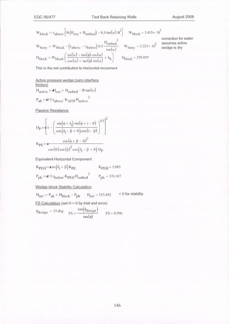
EQC 06/477 Tied Back Retaining Walls August 2008
Wblock =Yabove'B (1'exc+ Hembed - 0-5·tan(a)·1321 Wblock =3.453>< 103
Wbuoy Wblock - Yabove - Ybelow*5
Hembed
tan a
2
Wbuoy =
correction for water
3 assumes active3.221 x 10
wedge is dry
Hblock
:= W< sin(a) - tan(@·cos(a)
block- IC coscl + tan*·sina
+khJ Hblock - 299.()59
This is the net contribution to horizontal movement
Active pressure wedqe (zero interface
friction)
Hactive - embed_,1-'exc + H
Pah -'·5.Yabove KAE'-1.11
Passive Resistance
- 13·tan(a)
2
active
r sin* + ii)·sin(0 + i-0) 0-5Dp "11-1 3
l cos<6i-[1+ Ocos(i -p)jcos (0 +B- 0)2
KPE »1
cos(0)cos(11)2 cosJi -P+ 0·DpEquivalent Horizontal Component
KPE]-1 -cos <6i + [3 KI,E Xi)EH = 5.085P , = 376.107Pph "8.5-Ybelow K I1{I f Hembed pn
Wedge-block Stability Calculation
Hnet :- Pah + Hblock - Prh 1 Inet = 515.692 < 0 for stability
FS Calculation (set H=Oby trial and error)
lan*design¢'design = 35-deg IS:= FS = ().996
tan (44
146
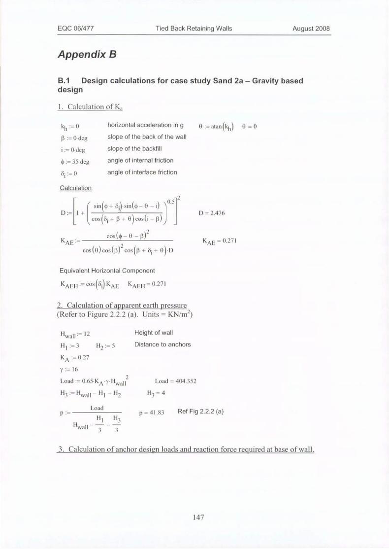
EQC 06/477 Tied Back Retaining Walls August 2008
Appendix B
B.1 Design calculations for case study Sand 2a - Gravity baseddesign
1. Calculation of K,
kh:= 0 horizontal acceleration in g 0:= atan (kB:= 0· deg slope of the back of the wall
i:= 0·deg slope of the backfill
¢:= 35·deg angle of internal friction
4-0 angle of interface friction
hJ 0=0
Calculation
r sin* + 6 sin(* -0-0 'D:= 1 +
l cosi +P + 0) cos(i -11)j
-2().5
D = 2.476
KA E ACOS (0 - 0
cos(O)cos(p)2 cos
'2
- P)K
(B + 61 + 0).DAE = 0.271
Equivalent Horizontal Component
KA F.1-1 := cos tii) KAIE KAE} 1 - 0.271
2. Calculation of apparent earth pressure
(Refer to Figure 2.2.2 (a). Units = KN/mb
Hwall:= 12 Height of wall11 1 :=3 1 12:-5 Distance to anchors
KA := 0.27
7:= 16
Load := 0.65·KA-7 Hwall2 Load = 4()4.352
113:= Hwall- 14 - 112 1-13=4
P:=
Il
p = 41.83 Ref Fig 2.2.2 (a)
wall
Load
Ill 113----I
3 3
3. Calculation of anchor design loads and reaction force required at base of wall.
147
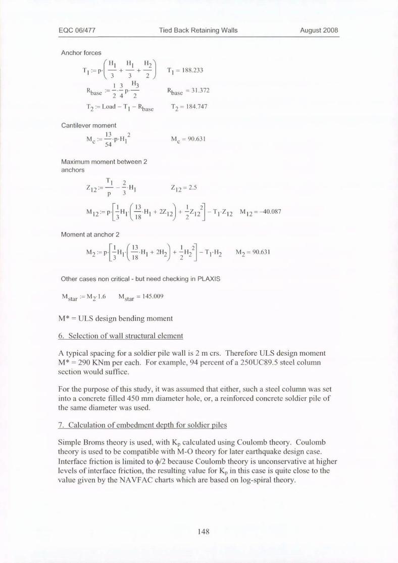
EQC 06/477 Tied Back Retaining Walls August 2008
Anchor forces
/ Hl 1-11 H2Tl:= p.1 -+-+-1 Tl= 188.233
43 3 27
Rbase i
1 3 H3R
24 2base = 31.372
T2 := Load - Ti - Rbase T2 = 184.747
Cantilever moment
13 2M..:=-.P Ill MC = 90.631
'- 54
Maximum moment between 2
anchors
Z
T
12 := -P
1 2-- -·H
1Z 12 '= 2.5
M 1.1'13-.11
*18+ 2Z 12 + iZ -T
1Z
12M
12'= -40.087
Moment at anchor 2
M
2:= P.L-1-13 11' 13-·H
*18+ 2112 + -74'2 -T I1
2M 2'= 9().631
Other cases non critical - but need checking in PLAXIS
Mstar := MIl.6 Mstar = 145.009
M* = ULS design bending moment
6. Selection of wall structural element
A typical spacing for a soldier pile wall is 2 m crs. Therefore ULS design moment
M* = 290 KNm per each. For example, 94 percent of a 250UC89.5 steel columnsection would suffice.
For the purpose of this study, it was assumed that either, such a steel column was setinto a concrete filled 450 mm diameter hole, or, a reinforced concrete soldier pile ofthe same diameter was used.
7. Calculation of embedment depth for soldier piles
Simple Broms theory is used, with Kp calculated using Coulomb theory. Coulombtheory is used to be compatible with M-0 theory for later earthquake design case.
Interface friction is limited to ¢/2 because Coulomb theory is unconservative at higherlevels of interface friction, the resulting value for Kp in this case is quite close to thevalue given by the NAVFAC charts which are based on log-spiral theory.
148
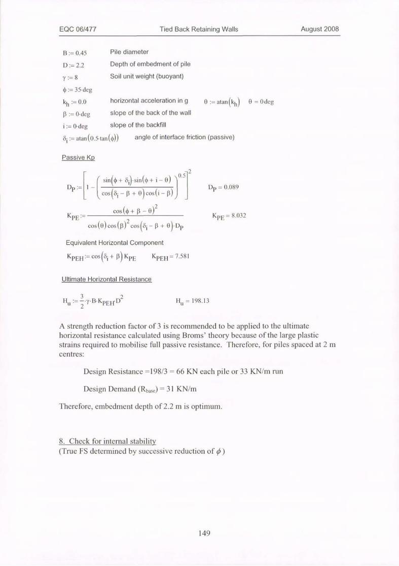
EQC 06/477 Tied Back Retaining Walls August 2008
B:= 0.45 Pile diameter
D:= 2.2 Depth of embedment of pile
7:=8 Soil unit weight (buoyant)
0 := 35·deg
kh:= 0.0 horizontal acceleration in g 0 := atan(kh)p:= 0·deg slope of the back of the wall
i:= 0·deg slope of the backfill
6i - atan 0.5- tan (*)) angle of interface friction (passive)
0 = Odeg
Passive Kp
f sin + tii) sin(* + i- 0) 0*5 2Dp:= 1 - Dp = ().()89
l cos <ai - P + 0 cos (i - 13) jcos (0 +B- 0)2
KPE:= KpE = 8.032cos(0)cos (Pfcosii -13 + 0·Dp
Equivalent Horizontal Component
KPEH := cos til + 13 Kpli KPEH=7.581
Ultimate Horizontal Resistance
H3
u := 278·KPEHD2
HU
=198.13
A strength reduction factor of 3 is recommended to be applied to the ultimatehorizontal resistance calculated using Broms' theory because of the large plasticstrains required to mobilise full passive resistance. Therefore, for piles spaced at 2 mcentres:
Design Resistance =198/3 = 66 KN each pile or 33 KN/m run
Design Demand (Rbase ) = 31 KN/m
Therefore, embedment depth of 2.2 m is optimum.
8. Check for internal stability
(True FS determined by successive reduction of 0)
149

EQC 06/477 Tied Back Retaining Walls August 2008
A
Wall- 1
H
I V
d
/ 14./.
4--Internal
Stability
/ ExternalStability
f
1
if
t
kh:= 0 horizontal acceleration in g 0 := atan (kh)13:= 0·deg slope of the back of the wall
i:= 0·deg slope of the backfill
0 := 27.(Adeg angle of internal friction
4 := atan(0.5-tan(0)) angle of interface friction (passive) 6
8 = 0 deg
a:-0
Calculation
2. 0.5
r sin* + Oasin(I) -0-i) 1D.= 1+1 , . /. D=2.155
lcos (ba +P+ 0 cosli -P)
Kcos(*-0- p)2
AE » KCOS (0)cos(pfcosp + 61 + 8 D
AE= 0.362
Equivalent Horizontal Component
KAEH - cos cia + 13) KAE KAEH = 0.362
Failure surface inclination
aa:=0-i-0 bb:-0-0-0 ec:=62 +P+0aa = 27.9deg bb = 27.9deg ce = 0 deg
PA 0 -0 + atan+an(aa)-(tan(aa) + cot(bb))·(1 + tan(cc)·cot(bb)) - tan(aa)1
1 + tan(ce)·(tan(aa) + cot(bb)) J
PA =58.95deg
150
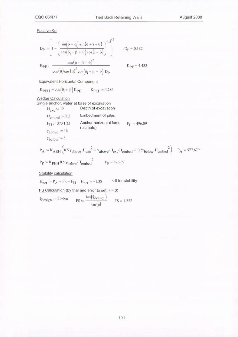
EQC 06/477 Tied Back Retaining Walls August 2008
Passive Kp
r sin + 6i·sin(0 +i-0) )0.5- 2Dp:= 1 - Dp = 0.1824 cos{6i -p + 0)cos(i -p)K
PE -
cos(0 +P- 0)2K
cos(0)cos (13)2 costii -13 + 0·DpPE-
4.433
Equivalent Horizontal Component
KpEH - cos i + 13 KPE KPEH = 4.286
Wedqe Calculation
Single anchor, water at base of excavation
' 'exe--12 Depth of excavation
' 'embed - 2.2 Embedment of piles
41 := 373· 1.33
Yabove := 16
Anchor horizontal force F
(ultimate)H-
= 496.()9
ybelow := 8
2 21PA r=KAF.Ill "exc | lexe Hembed + OYbelow'Hembed J PA = 577.679< 0.5·Yabove + 7 above
2 p = 82.969PP:= K[)141 1.0.5.Ybelowliembed
Stability calculation
Hnet - PA - PP - FH "net - -1.38 < 0 for stability
FS Calculation (by trial and error to set H = 0)
tan design 4)design = 35·deg FS := FS = 1.322
tan<*)
151

EQC 06/477 Tied Back Retaining Walls August 2008
9. Check for external stability
Wall-
H
U
d
Slid
bloc
f
a
/ Active/' wedge
ing:k t
1 ,V/
kh:= 0 horizontal acceleration in g 0 := atan (kh) 0 = 0 deg13:= 0·deg slope of the back of the wall
i:= 0. deg slope of the backfill
*:= 28·deg angle of internal friction
4 = atan(0.5·tan(*)) angle of interface friction (passive) t > OCalculation
2
1 0.5r sin + Ja*sin(0 -0-11D:= 1+| D = 2.159
K
l Cos (ba +P+O) cos (i -B)Jcos (0 -O - 13)2
AE i= KAE-().361
COS (0) COS (P)- COS 0+%+9.D
KAEH = cos cia + 13 KAE KAEH = 0.361 Equivalent Horizontal Component
Sliding block details
B:= 9.6 Breadth of block
a:=20. R deg Failure surface
11 -= 12 Depth of excavationeXC
"embed := 2.2 Embedment of piles
:= 16Y above8Ybelow »
152
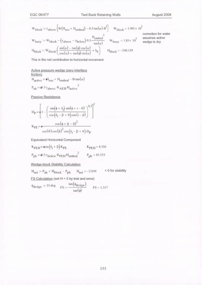
EQC 06/477 Tied Back Retaining Walls August 2008
Wblock := yabove-B·(Hexc + Hembed - 0.5-tan(a)·13 Wblock = 1.901 x '0
Wbuoy -
W block - <Yabove - Ybelow*.5"embed
tan (a
2
Wbuoy
1.85 x 10
correction for water
3 assumes active
wedge is dry
"block 2- W( sin(a - tan(0·cos(a
blockl i ,< Coslot) + tan¢·sina
+k 11h block -
-24().159
This is the net contribution to horizontal movement
Active pressure wedqe (zero interface
friction)
"act,ve exe„Iii +H
embed
Pah -0*5 Yabove KAEH' H
Passive Resistance
- B·tan(a)
2
active
C sin(¢+ 4)·sin((1)+i- 0) 10-5 2
DP -1 1 -1( cos (bi - p + 0 cos 0 - p) jcos(0 + 13 - 0)2
K pE :-1
cos(0)cos (13)2 cosfi -13+ O)·DP
Equivalent Horizontal Component
KE,EH -Ios (6i + P) KPE KpEH = 4.316
Prh -0.5-ybelow* KI,Ell- I lembed- Prh = 83.553
Wedqe-block Stabilitv Calculation
Hnet - Pah + Hblock - ph Hnet = -2.039 < 0 for stability
FS Calculation (set H=Oby trial and error)
¢ lesign = 35·deg FS := tan *desigi, FS= 1.317
tan (4))
153
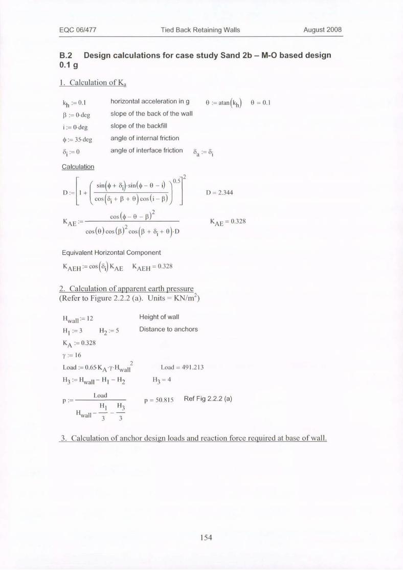
EQC 06/477 Tied Back Retaining Walls August 2008
B.2 Design calculations for case study Sand 2b - M-O based design0.1 g
1. Calculation of K.-
kh:= 0.1 horizontal acceleration in g
p := 0·deg slope of the back of the wall
i:= 0. deg slope of the backfill
¢ := 35·deg angle of internal friction
4-0 angle of interface friction 8
:= atan (k
1
hJ 0 -0.1
a
0
:= 6
Calculation
2
c sin<0 + 4)sill(0 -0-13 1D:= 1 + D = 2.344
C coscoi + B + 0)cos(i - p))cos (0 -0- p)2
KAE= KAE - 0.328cos(¢)) cos(13)2 cos[1 + 6i + 0·D
Equivalent Horizontal Component
KA'€11 - cos 8 KAE KAE]-1 = 0.328
2. Calculation of apparent earth pressure(Refer to Figure 2.2.2 (a). Units = KN/m2)
1-lwal]:= 12 Height of wall
[Il:= 3 H2:= 5 Distance to anchors
KA := 0.328
y:= 16
2
Load:=0.65·KA'7'11wallLoad = 491.213
"3 := Hwall- ill - }12 H3 = 4
P:=
H
Loadp = 50.815 Ref Fig 2.2.2 (a)
111 H3wall
3 3
3. Calculation of anchor design loads and reaction force required at base of wall.
154

EQC 06/477 Tied Back Retaining Walls August 2008
Anchor forces
<HI Hl H27
Tl := p.1 -+-+- 191 = 228.668£3 3 2
Rbase ;13
24
[13P- R
2base =
38.111
T2 := Load -Tl- Rbase 1,2 = 224.433
Cantilever moment
13 2
Mc:= fi-p-Ill Me = 110.099
Maximum moment between 2
anchors
Z
T
12.=P1 2- - -Ill
31 Z 12'= 2.5
M 12 =PIT" 1113-·H
l 81
+ 2Z 12 + tz 12-T Z
12M
12=-48.698
Moment at anchor 2
M2 ;= P ·I- H 12.HI8
1+ 2H2 + 1 1 1. 1 11
2M
2-= 110.099
Other cases non critical - but need checking in PLAXIS
Mstar = MI 1.6 M star= 176.159
M* = ULS design bending moment
6. Selection of wall structural element
A typical spacing for a soldier pile wall is 2 m crs. Therefore ULS design momentM* == 352 KNm per each. For example, 83 percent of a 3101-1096.8 steel columnsection would suffice.
For the purpose of this study, it was assumed that either, such a steel column was setinto a concrete filled 450 mm diameter hole, or, a reinforced concrete soldier pile ofthe saine diameter was used.
7. Calculation of embedment depth for soldier piles
Simple Broms theory is used, with Kp calculated using Coulomb theory. Coulombtheory is used to be compatible with M-0 theory for later earthquake design case.
Interface friction is limited to ¢/2 because Coulomb theory is unconservative at higherlevels of interface friction, the resulting value for Kp in this case is quite close to thevalue given by the NAVFAC charts which are based on log-spiral theory.
155

EQC 06/477 Tied Back Retaining Walls August 2008
B := 0.45 Pile diameter
D:= 2.5 Depth of embedment of pile
7 :=8 Soil unit weight (buoyant)
0 := 35·deg
kh := 0. 1 horizontal acceleration in g 0 := atan (kh)B:=0·deg slope of the back of the wall
i:= 0- deg slope of the backfill
Oi - atan(0.5·tan(*)) angle of interface friction (passive)
0 = 5.71 ldeg
Passive Kp
< sin((I) + til)·sin((I) +i-0) 0.5 2Dp:= 1-1 Dp = ().114l cos i - [3 + 0 cos (i - 13) K
COS (0 + 0 -PE:=
cos (O) cos (p)2 cos (6
,2
0J
i- P + 0)-DK
P
PE- 7.387
Equivalent Horizontal Component
KpEH = cos i + 11) KpE KpEH = 6.972
Ultimate Horizontal Resistance
II3
u :=27·B·KPENDz H
U= 235.313
A strength reduction factor of 3 is recommended to be applied to the ultimatehorizontal resistance calculated using Broms' theory because of the large plasticstrains required to mobilise full passive resistance. Therefore, for piles spaced at 2 mcentres:
Design Resistance =235/3 = 78 KN each pile or 39 KN/m run
Design Demand (Rbase) = 38 KN/m
Therefore, embedment depth of 2.5 m is optimuni.
8. Check for internal stability
(True FS determined by successive reduction oft)
156

EQC 06/477 Tied Back Retaining Walls August 2008
A
H
I
d
f
tI·45<&24#faX#*Elki
4-Internal /
/1 Stability ,/
f
/ External
Stability
oc
kh:= 0.1 horizontal acceleration in g 8 := atan(kh)13:= 0·deg slope of the back of the wall
i:= 0·deg slope of the backfill
¢:= 28.2·deg angle of internal friction
4 := atan(0.5-tan(*)) angle of interface friction (passive) 6
0 = 5.71 ldeg
a
Calculation
2
r si„C¢ + 3a)sin(* -0-i) 1D:= 1+| D = 2.034
< cos ba + P +8 COS (i -p)
KAE cos(4 -0- 0)2 K
cos(0) cos(Bfcos<B + tia + 0DAE-
= 0.424
Equivalent Horizontal Component
KAEH - cos6a + P KAE KAEH - 0-424
Failure surface inclination
aa:=4)-i-0 bb:= 0 - 13 - 0 ce:=tia+ B +0
aa = 22.489deg bb = 22.489deg ec = 5.71 ldeg
PA>¢-0 + atan4tan(aa)-(tan(aa) + cot(bb))·( 1 + tan(cc)·cot(bb)) - tan(aa)1
1 + tan(ce)·(tan(aa) + cot(bb))
PA= 54.17(xleg
157

EQC 06/477 Tied Back Retaining Walls August 2008
DP
2, 0.5
sinC* + 4)-sin(0 +i-0) 1:-1 - cos6i -B + eco(i _ p) DP== 0.222
KPE ·-
12COS (0 + 13 -03
K
cos(0)cos(Bfcos(6i -13 + 0·DpPE-
4.137
Equivalent Horizontal Component
KpEH - cos <6, + 13KPE KpF.H = 3.996
Wedqe Calculation
Single anchor, water at base of excavation
1-|ac= 12 Depth of excavation
Hembed := 2.5 Embedment of piles
FH :=453·1.33
Fabove := 16
Anchor horizontal force F
(ultimate)11-
= 602.49
tbelow = 8
2 2|A :== KAEI-1-(O'5.'labove 'Hexc + Yabove *1-|exc-'embed + O*57below Hembed PA = 702.38
2
Pp:= KPEHO.5.1/below Hembed Pp = 99.905
Stability calculation
|'net = PA - PP - Fll Hnet =-0.015 < 0 for stability
FS Calculation (by trial and error to set H = 0)
(1Uesign := 35·deg FS :- tan*design FS = ].306
tan(1))
158

EQC 06/477 Tied Back Retaining Walls August 2008
9. Check for external stability
H
I
d
t
Slidintblock
1 14
8 = 5.71 Ideg
1/V/
kh:= 0.1 horizontal acceleration in g 0 := atan (kh)B := 0·deg slope of the back of the wall
i:= 0·deg slope of the backfill
$ := 31.Rdeg angle of internal friction
Oi := atan(0.5·tan(*)) angle of interface friction (passive) % := OCalculation
2
< sin4) + 6a sin(0 -0-i) D:= 1 +f D= 2.198l cos (ba + B + 8) COS (i - 13)
KAE -cos(*- O-102
cos (0)cos(0)2 COS 0 + baK
+ oj·DAE-
0.371
KAEH := cosba + 13 KAE KAEH = 0.37' Equivalent Horizontal Component
Sliding block details
B:= 10.2 Breadth of block
a:=20.3-deg Failure surface
1-1 = 12 Depth of excavationexe
embed -= 2.5 Embedment of piles
Yabove := 1 6
Ybelow > 8
159

EQC 06/477 Tied Back Retaining Walls August 2008
Wblock > 7 above B· C Hexe + Hembed - 0-5·tan(a)·132 Wblock =
32.059x 10
Wbuoy
Hembed0.5.Wblock - (Yabove - Ybelow) tan<a
2
Wbuoy
correction for water
3 assumes active1.991 x 10
wedge is dry
Hr sinla) - tan(*)·cos(a)
block := *block ccoslot) + tan(0)·sin(a)+khi 1l
block --212.958
This is the net contribution to horizontal movement
Active pressure wedqe (zero interface
friction)
Hactive *"exc + Hembed - B·tan(ot)2
Pah -0 5 Yabove KAEH'Hactive
Passive Resistance
r sin + bi)·sin(0 +i-0) f.52DP -1 1 -1
C cos Cbi -P+ 0) cos(i -p)
KCON(*+ P -0)
PE;- 11.12 i
Cos(0)cos<B) cosld-
2
13 + 0)-D P
Equivalent Horizontal Component
KpEH -Ios (ji + 13 KPE KPEH = 5.266
2
Pph *u.5-7below*KPEHHembed pnP , = 131.65
Wedqe-block Stability Calculation
Hnet · Pah + Hblock - Pph 1|net = -3.436 < 0 for stability
FS Calculation (set H=Oby trial and error)
*design := 35·deg tan <4)design FS := FS = 1.129
tanct)
160
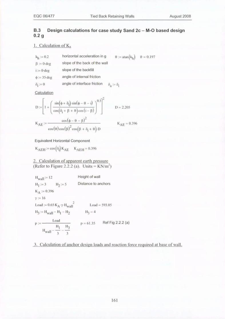
EQC 06/477 Tied Back Retaining Walls August 2008
B.3 Design calculations for case study Sand 2c - M-O based design0.2 g
1. Calculation of Ka
kh:= 0,2 horizontal acceleration in g
B := 0-deg slope of the back of the wall
i:= 0. deg slope of the backfill
¢ := 35·deg angle of internal friction
bi:= O angle of interface friction 8
:= atan k
1
hj 0 = 0.197
a
0
:= 6
Calculation
20.5
< sin(0 + 6il sin(0 -0-0 jD:-1+I ' I D= 2.205
l cos(bi +P+0 cos(i -p),cos (0 -0- p)2
KAE KAE = 0.396cos(0)cos (13)2 cos13 + bi + 0·D
Equivalent Horizontal Component
KAEH= costiKAE KAEH 0.396
2. Calculation of apparent earth pressure(Refer to Figure 2.2.2 (a). Units = KN/m2)
"wall - 12 Height of wall1 1 1 :=3 112 := 5 Distance to anchors
KA := 0.396
y:= 162
Load:=0.65·KA 7·HwallLoad = 593.05
1 13:=Hwall-Hl-H2 1 13 = 4
P:=
H
Load
HI Hwall
3 3
p = 61.35 Ref Fig 2.2.2 (a)3
3. Calculation of anchor design loads and reaction force required at base of wall.
161
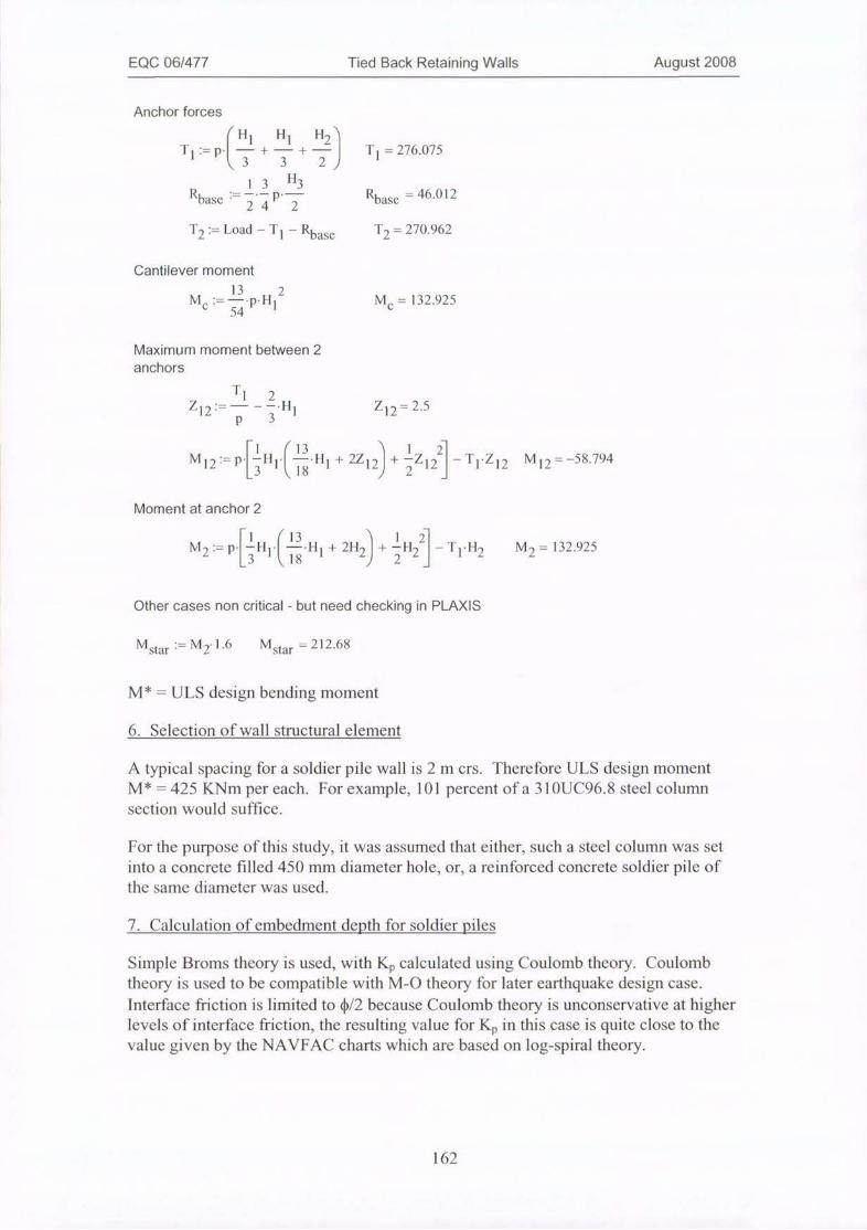
EQC 06/477 Tied Back Retaining Walls August 2008
Anchor forces
T
1:= P.l--31 11
3
1 [12 -+-IT
1)= 276.075
Rbase ·
1 3 H3R
24 2base -
46.012
T2 := Load -Tl- Rbase T2 = 270.962
Cantilever moment
13 2Mr:= -.p.111- 54
MC
= 132.925
Maximum moment between 2
anchors
7.
T
12 ---P
1 2---,11
31
Z12-
2.5
M 12 -P] THI.l,12.H<18
+ 2Z 121 + 4-Z 122 -T 1Z
12M
12-= -58.794
Moment at anchor 2
ME= P.1-4111' 13-·H
<18+ 2[1A + tH T
1H
2M
2= 132.925
Other cases non critical - but need checking in PLAXIS
M M = 212.68star := M21.6 star
M* = ULS design bending moment
6. Selection of wall structural element
A typical spacing for a soldier pile wall is 2 m crs. Therefore ULS design moment
M* == 425 KNm per each. For example, 101 percent of a 310UC96.8 steel columnsection would suffice.
For the purpose of this study, it was assumed that either, such a steel column was setinto a concrete filled 450 mm diameter hole, or, a reinforced concrete soldier pile ofthe same diameter was used.
7. Calculation of embedment depth for soldier piles
Simple Broms theory is used, with Kp calculated using Coulomb theory. Coulombtheory is used to be compatible with M-0 theory for later earthquake design case.
Interface friction is limited to ¢/2 because Coulomb theory is unconservative at higherlevels of interface friction, the resulting value for Kp in this case is quite close to thevalue given by the NAVFAC charts which are based on log-spiral theory.
162
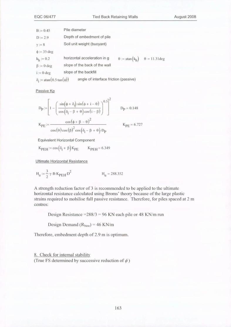
EQC 06/477 Tied Back Retaining Walls August 2008
B:= 0.45 Pile diameter
D:= 2.9 Depth of embedment of pile
7:=8 Soil unit weight (buoyant)
¢:=35·deg
kh:= 0.2 horizontal acceleration in g 0 := atan(kh) 0 - 11.3ldegB:= 0·deg slope of the back of the wall
i:= 0·deg slope of the backfill
4 := atan (0.5-tan (1))) angle of interface friction (passive)
Passive Kp
20.5ir sinl¢+bij.Sln<*+ 1-0) 1
DP:= 1-1 Dp = 0.148l cos bi -P+0 cos(i -13)jK
COS(0 + B -0)PE -
cos(0) cos (p)2 cos(di -
2
K
P + 0).1)PPE'= 6.727
Equivalent Horizontal Component
KpEH:= cos fi + 13) KPE KpE.11 = 6.349
Ultimate Horizontal Resistance
H3
u -Z*Y*13. KPEH D2
Hu:= 288.352
A strength reduction factor of 3 is recommended to be applied to the ultimate
horizontal resistance calculated using Broms' theory because ofthe large plastic
strains required to mobilise full passive resistance. Therefore, for piles spaced at 2 mcentres:
Design Resistance =288/3 = 96 KN each pile or 48 KN/m run
Design Demand (Rbuse ) = 46 KN/m
Therefore, embedment depth of 2.9 m is optimum.
8. Check for internal stability
(True FS determined by successive reduction oft)
163
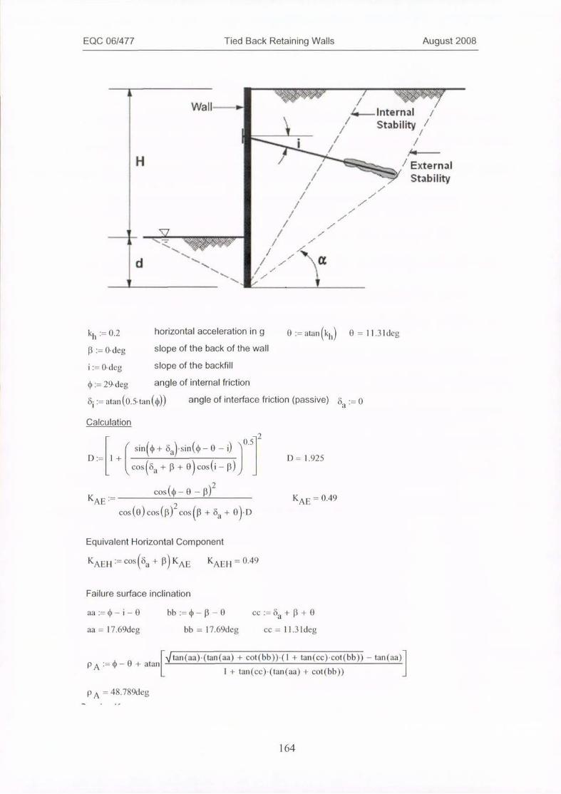
EQC 06/477 Tied Back Retaining Walls August 2008
A
Wall--
H
IU
d
49#349*W i b/b:&<&:.'*-"'/
4.--Internal /
Stability //
M#
T/ -,Sk:k: l External
3* Stability
t
0 = 11.31 deg
// la
kh:= 0.2 horizontal acceleration in g 0 := atan(kh)p:= 0· deg slope of the back of the wall
i:= ()· deg slope of the backfill
0:= 29·deg angle of internal friction
4 = atan(0.5·tan(¢)) angle of interface friction (passive) 8a'
=0
Calculation
2.0.5
r sin* + 63'sin(0 -0-i) 1D:= 1+I D = 1.925
<coscoa +P+ 0)costi -13)
Kcos 61)-0- p)2
AE Ki 12
COS (0)cos<B) cos<13 + Oa + eDAE
Equivalent Horizontal Component
K/\Ell :=costia + PKAE KAEI-1 049
Failure surface inclination
aa:-0-i-0 bb:=0-0-0 CC := 4 +P+0
aa = 17.69deg bb = 17.69deg ce = 11.3 ldeg
PA = 0-0 + atan+an(aa)·(tan(aa) + cot(bb))·(1 + tan(ce)·cot(bb)) - tan(aa)
1 + tan(cc)·(tan(aa) + cot(bb))
PA =48.789deg
164

EQC 06/477 Tied Back Retaining Walls August 2008
Passive Kp
< sin((1) + bij·sin(0 + i - 0) jo.5 2DP:= 1 -1 , / Dp = 0.262l cosai -P+0 cos(i - 13)KPE:=
cos(4,+11-0)2K
cos (0) cos (13)2 cos 6· - p + 0· Dp1
PE-3.963
Equivalent Horizontal Component
KPEN - cos6i + P KPE KpEH = 3.819
Wedqe Calculation
Single anchor, water at base of excavation
H. '= 12 Depth of excavationexe
Hembed := 2.9 Embedment of piles
FH := 547·1.33
·= 16Yabove
Anchor horizontal force F
(ultimate)H'= 727.51
Ybelow - 8
2 + 0.57belowPA-=KAE[1<05.'tabove*Hexc + Yabove Hexc'Hembed2
pp := KPE' 1.0.5.ybelow'Hembed Pp = 128.468
Stability calculation
embed2 PA-
= 854.253
Hnet -PA - PP - FH "net - -1.725 < 0 for stability
FS Calculation (by trial and error to set H = 0)
tan*design *design := 35-degFS := FS = 1.263
tan (0)
165
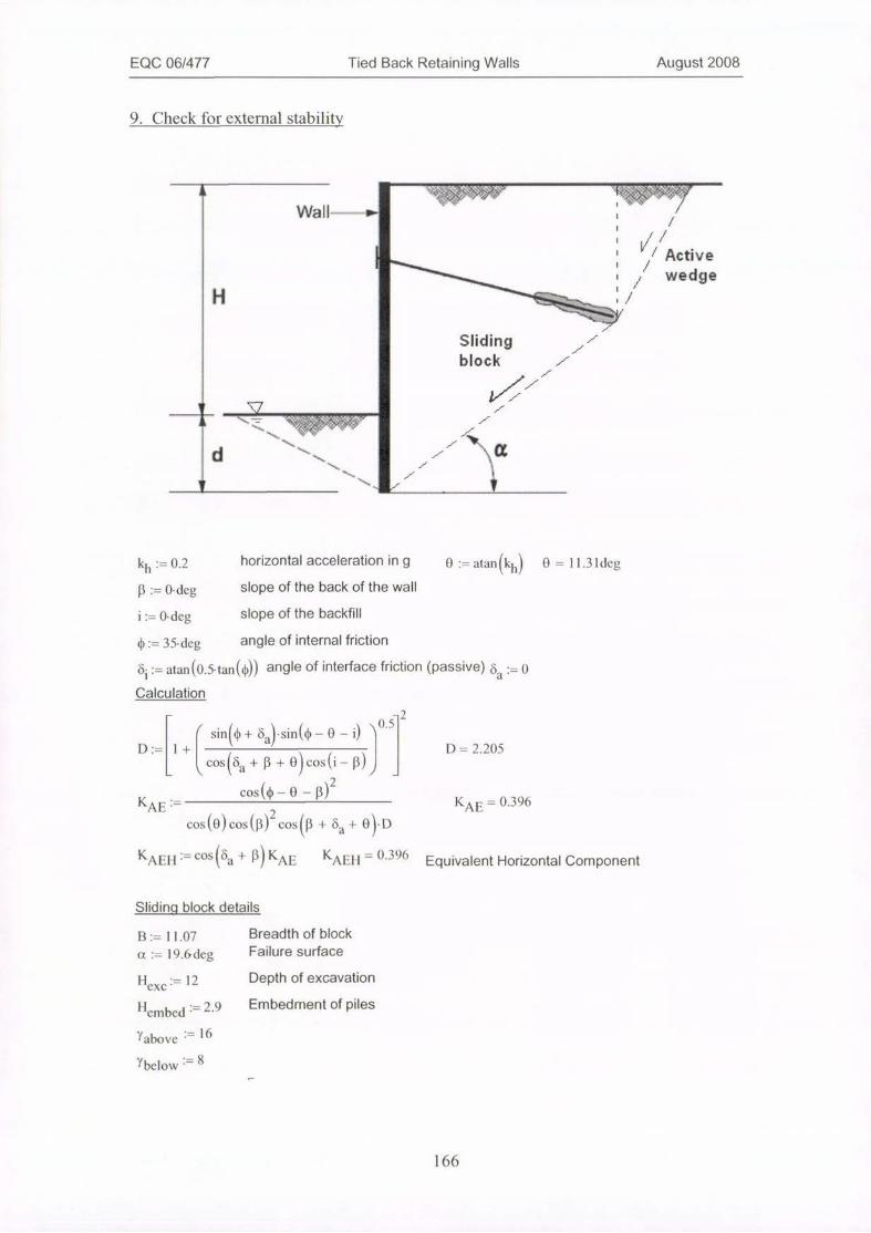
EQC 06/477 Tied Back Retaining Walls August 2008
9. Check for external stability
A
Wall-,---
H
I U
71.9
d
4524:0«%*0'1
77.17,0
/ f
/. j
Sliding
kh:= 0.2 horizontal acceleration in g 0 := atan(kh)p:= 0· deg slope of the back of the wall
i:= 0·deg slope of the backfill
0 := 35·deg angle of internal friction
6i := atan(0.5-tan(0)) angle of interface friction (passive) ba := 1Calculation
r sin0 + tiasin(0 -0-i) 1D:= 1+I \/\ D = 2.205
l cos(ia +P+ 0)cos li -B)
Kcos (0 -0- p)2
AE- K4.12 1cos(0)cosill) coslp + 6&+ 0) L)
AE-0.396
KAEI' - costia + 13 KAE KAEH = 0.396 Equivalent Horizontal Component
Sliding block details
B := 11.07 Breadth of block
a := 19.(>deg Failure surface
11 -= 12 Depth of excavationexe*
Hembed := 2.9 Embedment of piles
Yabove » 16Ybelow = 8
0 = 11.3ldeg
block
V
0
166
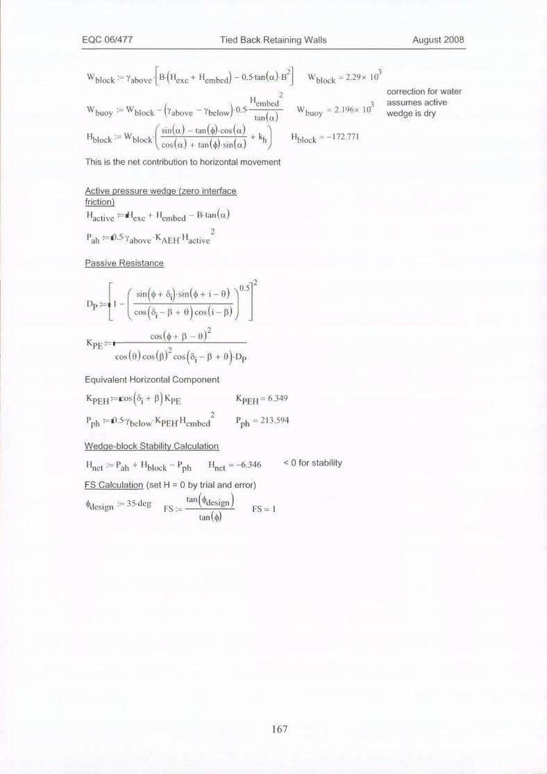
EQC 06/477 Tied Back Retaining Walls August 2008
3Wblock := Yabove B.(1'exc + Hembed - 0.5·tan(a)·B Wblock = 2.29>< 10
Wbuoy
WHembed
block - Yabove - Ybelow) 0.5 tan a
2
Wbuoy
correction for water
3 assumes active2.196x 10
wedge is dry
< sin(a) - tan(@·cos(a)Hblock := Wblock* cos(a) + tan(0)·sin(a)
+kh Hblock = -172.771
This is the net contribution to horizontal movement
Active pressure wedqe (zero interface
friction)
- B·tan(ot)Hactive -'Hexc + Hembed
2
Pah *'*5.Yabove'KAEH*Hactive
Passive Resistance
2, 0.5
C sin(* + fi) sin(4 + i- 0) 1Dpil- 1
( cos <6i -P+ 0 cos (i - p) j
cos (0 +B- 0)2KPE:-1
cos (0) cos ([3)2 cosi - P + 0)·DPEquivalent Horizontal Component
KPEI-1 =Cos 6i + 13 KPE KPEH = 6.349
Pph -D.5.ybelow KPE]-1- Hembed2 Pph = 213.594
Wedqe-block Stability Calculation
Hnet = Pah + Hblock - Pph Hnet - -6.346 < 0 for stability
FS Calculation (set H=Oby trial and error)
tandesign*design ,= 35·deg FS := FS = 1
tan (40
167

EQC 06/477 Tied Back Retaining Walls August 2008
Appendix C
C.1 Design calculations for case study Sand 3a - Gravity baseddesign
Steps 1 to 8 same as for Sand 28.
9. Check for external stability
Sliding
t
1a
= atano© 0 = Odeg
1
41,/ Active
wedge
block
kh:= 0 horizontal acceleration in g o:
p :=0· deg slope of the back of the wall
i:= 0·deg slope of the backfill
0 := 26.7-deg angle of internal friction
4 - atan(0.5·tan(*)) angle of interface friction (passive) := OCalculation
-2
/ sin(4) + tia sin(0 -0-i) )D:= 1+I D=2.101
l cos(c;a +P+ o) cos(i -[1) K
COS (0-0AE =
COS (0)cos([3)2 COS
/-
P)2K
B + fa + 0- DAE= 0.38
KAE}-1 -= cosba + 13 KAE KAEH = 0.38 Equivalent Horizontal Component
A.4
H
I
d
168

EQC 06/477 Tied Back Retaining Walls August 2008
Sliding block details
B:=10.14 Breadth of block
a:= 19·deg Failure surface
Hexc - 12 Depth of excavation
Hembed = 2.2 Embedment of piles
Yabove := 16
Ybelow := 8
W block = Yabove B.(Hexe
+ 11embed) - 0.5-tan(a)·82- Wblock -
32.()21 x 10
Wbuoy -
W
Hembed
block - 7above - Ybelowf·5 Mn(a)
2
Wbuoy
31.964 x 10
correction for water
assumes active
wedge is dry
Hblock = W< sinux) - tan(¢)·cos(a)
block'|C cos((i + tan*·sin(a
+khj Hblock -
-273.193
This is the net contribution to horizontal movement
Active pressure wedqe (zero interface
friction)
i lactive -ilexc + i lembed - B·tan(a)2
Pah *').5.Yabove KA[ill l|active
Passive Resistance
f sin(4) + 4)·sin(0 +i-0) 10.5 2Dp -1 1 -1 3
l cos(4-P+0) cos(i -p)
cos(*+P- 0)2KpE :-1
Cos(0)cos ([1)Zeosi -13 + 0·Dp
Equivalent Horizontal Component
KPEI-1 *Ios (bi + 1-3 KpE2
Pph -').5.7below- KPE[1 i lembed
KPEH= 3.947
P h = 76.406P
Wedqe-block Stability Calculation
' 'net = block - Pph H = -1.033 < 0 for stabilityah + 11 net
FS Calculation (set H=Oby trial and error)
ciesign := 35·deig tati *design FS:= FS = 1.392
ton((10
169

EQC 06/477 Tied Back Retaining Walls August 2008
C.2 Design calculations for case study Sand 3b - M-0 based design0.1 g
Steps 1 to 8 same as for Sand 2b.
9. Check for external stability
A
Wall --
/ Active
/1 wedgeH
Sliding f
block
1 iV/
I 7
d
t
kh:= 0.1 horizontal acceleration in g 0 := atan (kh) 0 = 5.71 IdegB :=0·deg slope of the back of the wall
i:= 0. deg slope of the backfill
0 :=30.6deg angle of internal friction
fi - atan(0.5-tan(*)) angle of interface friction (passive) 8a :- 0Calculation
-2
r sin* + Oa*sin(I) -0-i) D:= 1 + D = 2.143
l cosfa +B+ e) cos (i -p) cos (0 -0- p)2
KAE > KAE < 0.388
COS(0)COS(p)£ COSB + ba + eDKAE'-1 = cosa + KAE KAEH = 0.388 Equivalent Horizontal Component
170
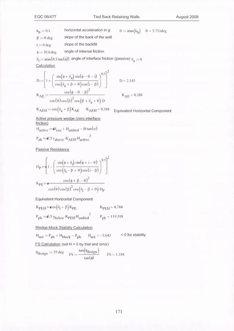
EQC 06/477 Tied Back Retaining Walls August 2008
kh := 0.1 horizontal acceleration in g 8 := atan(kh) 0 = 5.71 Ideg13 := 0·deg slope of the back of the wall
i:= 0. deg slope of the backfill
¢ := 30.Adeg angle of internal friction
Ji - atan(0.5·tan(¢)) angle of interface friction (passive) ba :- OCalculation
r sin(0 + 6:1)'sin(0 -0-i) 10.52
D:= 1 + D=2.143
l cos(tia +B+ 0)cos(i -p) cos(0 -0- 0)2
KAE:== KAE= 0.388cos(0)cos (13)2 cos<[1 + Oa + 0·D
1<Alill -=cos6:1 + |) KAE KAEH = 0·388 Equivalent Horizontal ComponentActive pressure wedge (zero interface
friction)
"active Al|exc + Hembed - B·tan(a)2
Pah -0.5.Yabove-KA[€11'Hactive
Passive Resistance
r sinC* + bj·sin(0 +i- 0) OI52Dp -0 1 -
C cosCii-B + 0)cos(i-B))cos (0 +P- 0)2
KPE >1
CoS (0) CoS (p)Lcosdi -P+ 0·Dp
Equivalent Horizontal Component
Kptil-1 *costii + [3 KPE KPEH= 4.784
2
Prh *85·7below KPE}r lk'embed Pph = 119.598
Wedge-block Stability Calculation
"net = Pah + Hblock - Prh Hnet =-5.643 < 0 for stability
FS Calculation (set H=Oby trial and error)
t.111 ¢design *design := 35-deg FS := FS= 1.184
tan(0)
171
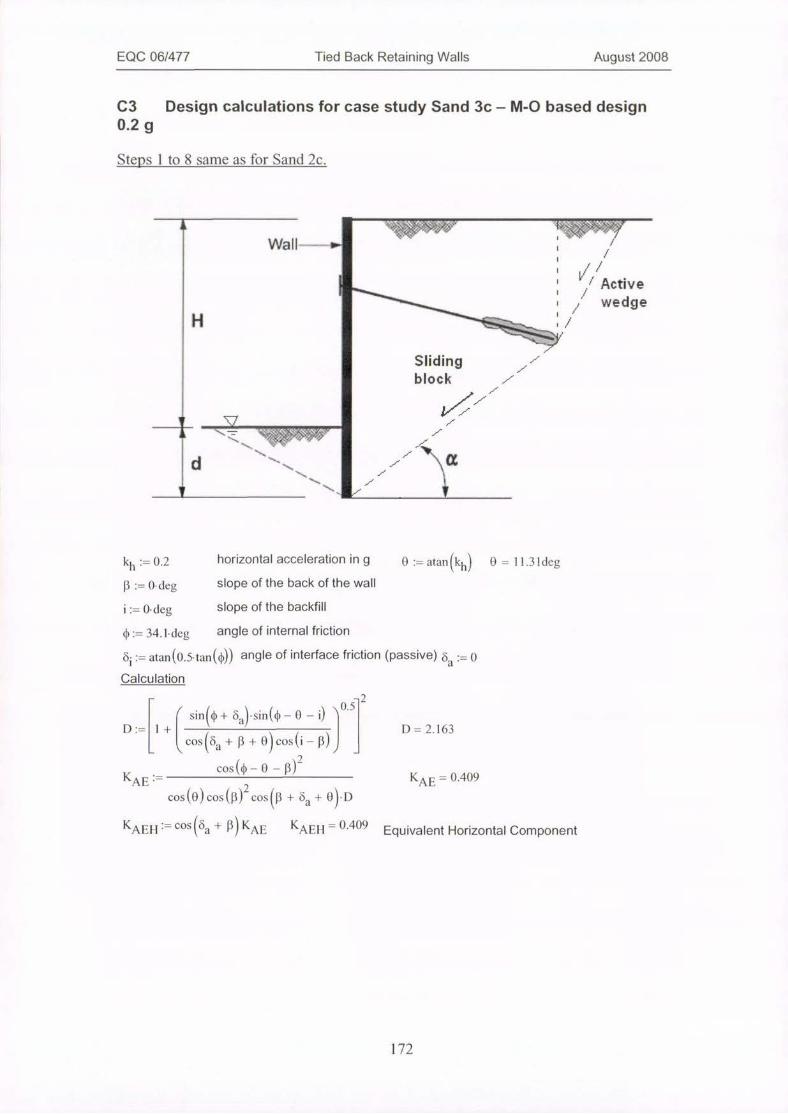
EQC 06/477 Tied Back Retaining Walls August 2008
C3 Design calculations for case study Sand 3c - M-0 based design0.2 g
Steps 1 to 8 same as for Sand 2c.
A
Wall--- 1
H
I U
dt
Slid
bloc
t
f
a
kh:= 0,2 horizontal acceleration in g 0 :=atan(kh) 0= 11.3 ldegslope of the back of the wall
i:= 0·deg slope of the backfill
¢:= 34.1·deg angle of internal friction
6i := atan(0.5·tan(@) angle of interface friction (passive) 6 :- 0Calculation
2
< sin* + 6asin(*-0 -i) 1D:= 1+I D = 2.163
l cos(tia + 13 + 0)Cosli - B)
Kcos (0-0 - p)2
AE- K
cos(0)cos(11)2 cos13 + 68 + 8) I)AE-
0.409
KAHN - costia + 13 KAE KAEII = 0.409 Equivalent Horizontal Component
· Active
/' wedge\ j
-7
ingj
:k
1 iV/
172
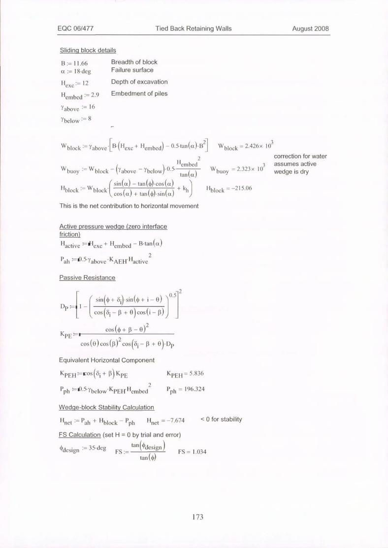
EQC 06/477 Tied Back Retaining Walls August 2008
Sliding block details
B := 11.66 Breadth of block
a:= 18·deg Failure surface
Hexc ·= 12 Depth of excavation
Hembed .= 2.9 Embedment of piles
Yabove - 16
ybelow = 8
B·(Hexc + Hembed - 0.5-tan(00·B Wblock = 2.426x 10³Wblock := Yabove L
Wbuoy
:= WHembed
block - above - Ybelow)-05 4tan la)
2
Wbuoy
correction for water
3 assumes active= 2.323 x 10
wedge is dry
Hblock = Wr sin(a) - tan((b-cos(a)
blockC cos(a) + tan(0)·sirdol)
+kh Hblock = -215.06
This is the net contribution to horizontal movement
Active pressure wedqe (zero interface
friction)
Hactive - d 'exc + "enibeci - B·tan (a)2
P,ah -')5 Yabove KAEH llactive
Passive Resistance
DP xC sinpl) + 60.sin(0 +i-0) 0.5-211-1l cos bi -P + 0 codi - 13) 7
KCOS(*+P-0)
PE * 1
cos (O) cos (p )2 cos bi -
2
13 + 0).DP
Equivalent Horizontal Component
Kptil-':==,os6i + 13KPE KPEH= 5.836
2
P'111 -,15-Ybelow KPEH Hembed Pph = 196.324
Wedqe-block Stability Calculation
Hnet ·- Pah + Hblock - Pph Hnet = -7.674 < 0 for stability
FS Calculation (set H=Oby trial and error)
¢design := 35·deg FS -= tari *design FS = 1.034
tan ¢
173
Related Documents