FINANCIAL MATHEMATICS A Practical Guide for Actuaries and other Business Professionals Second Edition CHRIS RUCKMAN, FSA, MAAA JOE FRANCIS, FSA, MAAA, CFA Study Notes Prepared by Kevin Shand, FSA, FCIA Assistant Professor Warren Centre for Actuarial Studies and Research

Welcome message from author
This document is posted to help you gain knowledge. Please leave a comment to let me know what you think about it! Share it to your friends and learn new things together.
Transcript

8/8/2019 3500145 Financial Math for Actuary and Businessman
http://slidepdf.com/reader/full/3500145-financial-math-for-actuary-and-businessman 1/181
FINANCIAL
MATHEMATICS
A Practical Guide for Actuaries
and other Business Professionals
Second Edition
CHRIS RUCKMAN, FSA, MAAA
JOE FRANCIS, FSA, MAAA, CFA
Study Notes Prepared byKevin Shand, FSA, FCIA
Assistant Professor
Warren Centre for ActuarialStudies and Research

8/8/2019 3500145 Financial Math for Actuary and Businessman
http://slidepdf.com/reader/full/3500145-financial-math-for-actuary-and-businessman 2/181

8/8/2019 3500145 Financial Math for Actuary and Businessman
http://slidepdf.com/reader/full/3500145-financial-math-for-actuary-and-businessman 3/181
ExercisesandSolutions .................................... 121
6 Financial Instruments 1326.1 TypesofFinancialInstruments ............................. 132
6.1.1 MoneyMarketInstruments ........................... 1326.1.2 Bonds ....................................... 1336.1.3 CommonStock.................................. 1336.1.4 PreferredStock.................................. 1346.1.5 Mutual Funds . . . . ............................... 1346.1.6 GuaranteedInvestmentContracts(GIC).................... 1346.1.7 DerivativeSercurities .............................. 135
6.2 BondValuation...................................... 1376.3 StockValuation...................................... 148ExercisesandSolutions .................................... 149
7 Duration, Convexity and Immunization 1567.1 PriceasaFunctionofYield............................... 156
7.2 ModifiedDuration .................................... 1567.3 MacaulayDuration.................................... 1577.4 E ectiveDuration .................................... 1597.5 Convexity......................................... 159
7.5.1 MacaulayConvexity ............................... 1607.5.2 E ectiveConvexity................................ 160
7.6 Duration,ConvexityandPrices:PuttingitallTogether ............... 1607.6.1 RevisitingthePercentageChangeinPrice................... 1607.6.2 ThePassageofTimeandDuration....................... 1617.6.3 PortfolioDurationandConvexity........................ 161
7.7 Immunization....................................... 1627.8 FullImmunization .................................... 166ExercisesandSolutions .................................... 167
8 The Term Structure of Interest Rates 1778.1 Yield-to-Maturity..................................... 1778.2 SpotRates ........................................ 177
2

8/8/2019 3500145 Financial Math for Actuary and Businessman
http://slidepdf.com/reader/full/3500145-financial-math-for-actuary-and-businessman 4/181
1 Interest Rates and FactorsOverview
– interest is the payment made by a borrower (i.e. the cost of do ing business) for using alender’s capital assets (usually money); an example is a loan transaction
– interest rate is the percentage of interest to the capital asset in question – interest takes into account the risk of default (risk that the borrower can’t pay back the loan) – the risk of default can be reduced if the borrower promises to release an asset of theirs in the
event of their default (the asset is called collateral)
1.1 InterestInterest on Savings Accounts
– a bank borrows a depositor’s money and pays them interest for the use of their money – the greater the need for money, the greater the interest ra te o ered
Interest Earned During the Period t to t + s : AV - AV
t + s t – the Accumulated Value at time n is denoted as AV n
– interest earned during a period of time is the di erence between the Accumulated Value atthe end of the period and the Accumulated Value at the beginning of the period
TheE ectiveRateofInterest: i – i is the amount of interest earned over a one-year period when 1 is invested – i is also defined as the ratio of the amount of Interest Earned during the period to the
Accumula ted Value at the beginning of the periodAV - AV
t + 1 t i = AV
t
Interest on Loans – compensation a borrower of capital pays to a lender of capital – lender has to be compensated since they have temporarily lost use of their capital – interest and capital are almost always expressed in terms of money
2

8/8/2019 3500145 Financial Math for Actuary and Businessman
http://slidepdf.com/reader/full/3500145-financial-math-for-actuary-and-businessman 5/181
1.2 Simple Interest – let the interest amount earned each year on an investment of X be constant where the annual
rate of interest is i :AV = X (1 + ti ) ,
t
where (1 + ti ) is a linear function – simple interest has the pro perty that interest is NOT reinvested to ea rn additiona l interest – amount of Interest Earned to time t is
I = AV - AV = X (1 + it ) - X = X · it t 0
1.3 Compound Interest – let the interest amo unt earned each yea r on an investment of X also allow the interest earned
to earn interest where the annual rate of interest is i :
AV = X (1 + i ) , t
t
where (1 + i ) is an exponential function t
– compound interest produces larger accumulations than simple interest when t> 1 – note that a constant rate of compound interest implies a constant e ective rate of interest
1.4 Accumulated ValueAccumulated Value Factor: AV F
t
– assume that AV is continuously increasingt
–let X be the initial Principal invested ( X> 0) where AV = X 0
– AV defines the Accumulated Value that amount X grows to in t yearst
– the Accumulated Value at time t is the product of the initial capital investment of X (Prin-cipal) made at time zero and the Accumulation Value Factor:
AV = X · AV F ,t t
where AV F =(1+ it ) if simple interest is being applied and AV F =(1+ i ) if compound t
t t
interest is being applied
3

8/8/2019 3500145 Financial Math for Actuary and Businessman
http://slidepdf.com/reader/full/3500145-financial-math-for-actuary-and-businessman 6/181
1.5 Present ValueDiscounting
– Accumula ted Value is a future value pertaining to payment(s) made in the past – Discounted Value is a present value pertaining to payment(s) to be made in the future – discounting determines how much must be invested initially ( Z )sothat X will be accumu-
lated after t yearsX
Z · (1 + i ) = X Z = = X (1 + i ) t -t
(1 + i ) t
– Z represents the present value of X to be paid in t years
–let v = 1 , v is called a discount factor or present value factor 1+ i
Z = X · v t
Discount Function (Present Value Factor): PVF
t
– simple interest: PVF = 1t 1+ it
t – compound interest: PVF = 1 = v t t (1 + i )
– compound interest produces smaller Discount Values tha n simple interest when t> 1
4

8/8/2019 3500145 Financial Math for Actuary and Businessman
http://slidepdf.com/reader/full/3500145-financial-math-for-actuary-and-businessman 7/181
1.6 Rate of Discount: d Definition
– an e ective rate of interest is taken as a percentage of the balance at the beginning of theyear, while an e ective rate of discount is at the end of the year.
– eg. if 1 is invested and 6% interest is paid at the end of the year, then the AccumulatedValue is 1.06
– eg. if 0.94 is invested after a 6% discount is paid at the beginning of the year, then theAccumulated Value at the end of the year is 1.00
– d is also defined as the ratio of the amount of interest (amount of discount) earned duringthe period to the amount invested at the end of the period
AV - AV t + 1 t d = AV
t + 1
– if interest is constant, then discount is constant – the amount of discount earned from time t to t + s is AV - AV
t + s t
Relationships Between i and d – if 1 is borrowed and interest is paid at the beginning of the year, then 1 - d remains – the accumulated value of 1 - d at the end of the year is 1:
(1 - d )(1 + i )=1
– interest rate is the ratio of the discount paid to the amount at the beginning of the period:d
i =1 - d
– discount rate is the ratio o f the interest paid to the amount at the end of the period:i
d =1+ i
– the present value of end-of-year interest is the discount paid at the beginning of the year iv = d
– the present value of 1 to be paid at the end o f the year is the same as borrowing 1 - d andrepaying 1 at the end o f the year (if both have the same value at the end o f the year, thenthey have to have the same value at the beginning of the year)
1 · v =1 - d
– the di erence between end-of-year, i , and beginning-of-year interest, d , depends on the di er-ence that is borrowed at the beginning of the year and the interest earned on that di erence
i - d = i [1 - (1 - d )] = i · d = 0
5

8/8/2019 3500145 Financial Math for Actuary and Businessman
http://slidepdf.com/reader/full/3500145-financial-math-for-actuary-and-businessman 8/181
Discount Factors: PVF and AV F t t
– under the simple discount model the Discount Present Value Factor is:
PVF =1 - dt for 0 = t< 1 /d t
– under the simple discount model the Discount Accumulated Value Factor is:
AV F =(1 - dt ) for 0 = t< 1 /d - 1t
– under the compound discount model, the Discount Present Value Factor is:
t PVF =(1 - d ) = v for t = 0 t
t
– under the compound discount model, the Discount Accumulated Value Factor is:
- t AV F =(1 - d ) for t = 0t
– a constant rate of simple discount implies an increasing e ective rate of discount – a constant rate of compound discount implies a constant e ective rate of discount
6

8/8/2019 3500145 Financial Math for Actuary and Businessman
http://slidepdf.com/reader/full/3500145-financial-math-for-actuary-and-businessman 9/181
1.7 Constant Force of Interest: d Definitions
– annual e ective rate of interest is applied over a o ne-year period – a constant annual force of interest can be a pplied over the smallest sub-period imaginable
(at a moment in time) and is denoted as d – an instantaneous change at time t , due to interest rate d , where the accumulated value at
time t is X , can be defined as follows:d
t dtAV d =
AV t
d = ( AV )
t dt lnd
(1 + i ) t
dtX = X (1 + i ) t
i ) · ln (1 + i ) t
= (1 +(1 + i ) t
d = ln (1 + i )
– taking the exponential function of d results in
e =1+ i d
– taking the inverse of the above formula results in
e = 1 = v -d
1+ i
– Accumula ted Value Factor ( AV F ) using constant fo rce of interest ist
AV F = e d t
t
–PresentValueFactor( PVF ) using constant force of interest ist
PVF = e - dt
t
7

8/8/2019 3500145 Financial Math for Actuary and Businessman
http://slidepdf.com/reader/full/3500145-financial-math-for-actuary-and-businessman 10/181
1.8 Varying Force of Interest
– let the constant force of interest d now vary at each infitesimal point in time and be denotedas d
t
– a change from time t to t , due to interest rate d , where the accumulated value at time t 1 2 t 1
is X , can be defined as follows:d
t dt AV d =
t AV t
d = ( AV )
t dt lnd t t
2 2
d · dt = ( AV ) · dt t t dtln
t t 1 1
= ln ( AV ) - ln ( AV )t t
2 1
t 2
t d · dt = ln AV 2
t AV t t
1 1
t 2
d · dt AV t
t e = t 2
1 AV t
1
Varying Force of Interest Accumulation Factor - AV F t ,t
1 2
–let
t 2
d · dt t
AV F = e t
t , t 1
1 2
represent an a ccumulation factor over the perio d t to t , where the fo rce of interest is varying1 2
t
d · dt t
–if t = 0, then the notation simplifies from AV F to AV F i.e. AV F = e0 1 0 , t t t
2
–if d is readily integrable, then AV F can be derived easilyt t , t
1 2
–if d is not readily integrable, then approximate methods of integration are requiredt
Varying Force of Interest Present Value Factor - PVF t , t
1 2
–lett 2
d · dt AV - t
t PVF = 1 = 1 = = e 1 t
t , t 1 AV F AV t 1 2
2 t ,t t d · dt 1 2 2
t
e t 1
represent a present value f actor over the period t to t , where the force o f interest is varying1 2
t
d · dt - t
–if t = 0, then the notation simplifies from PVF to PVF i.e. PVF = e0 1 0 ,t t t
2
8

8/8/2019 3500145 Financial Math for Actuary and Businessman
http://slidepdf.com/reader/full/3500145-financial-math-for-actuary-and-businessman 11/181
1.9 Discrete Changes in Interest Rates – the most common application of the accumulation and present value factors over a period of
t years ist
AV F = (1 + i )t k
k = 1
andt 1
PFV =t (1 + i )
k k = 1
where i is the constant rate of interest between time k - 1andtime k k
9
8/8/2019 3500145 Financial Math for Actuary and Businessman
http://slidepdf.com/reader/full/3500145-financial-math-for-actuary-and-businessman 12/181
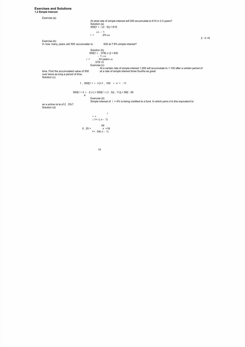
Exercises and Solutions1.2 Simple Interest
Exercise (a)At what rate of simple interest will 500 accumulate to 615 in 2.5 years?Solution (a)500[1 + i (2 . 5)] = 615
615 - 1i = . 2% 500
2 . 5 =9Exercise (b)In how many years will 500 accumulate to 630 at 7.8% simple interest?
Solution (b)500[1 + . 078( n )] = 630
- 1 6 30
i = . 33 years5 00
. 078 =3Exercise (c)
At a certain rate of simple interest 1,000 will accumulate to 1,100 after a certain period of time. Find the accumulated value of 500 at a rate of simple interest three fourths as greatover twice as long a period of time.Solution (c)
1 , 000[1 + i · n ]=1 , 100 i · n = . 11
500[1 + 3 i · 2 n ] = 500[1 + (1 . 5)( . 11)] = 582 . 504
Exercise (d)Simple interest of i = 4% is being credited to a fund. In which perio d is this equivalent to
an e ective ra te of 2 . 5%?Solution (d)
i i =n 1+ i ( n - 1)
. 040 . 25 = n =16
1+ . 04( n - 1)
10
8/8/2019 3500145 Financial Math for Actuary and Businessman
http://slidepdf.com/reader/full/3500145-financial-math-for-actuary-and-businessman 13/181
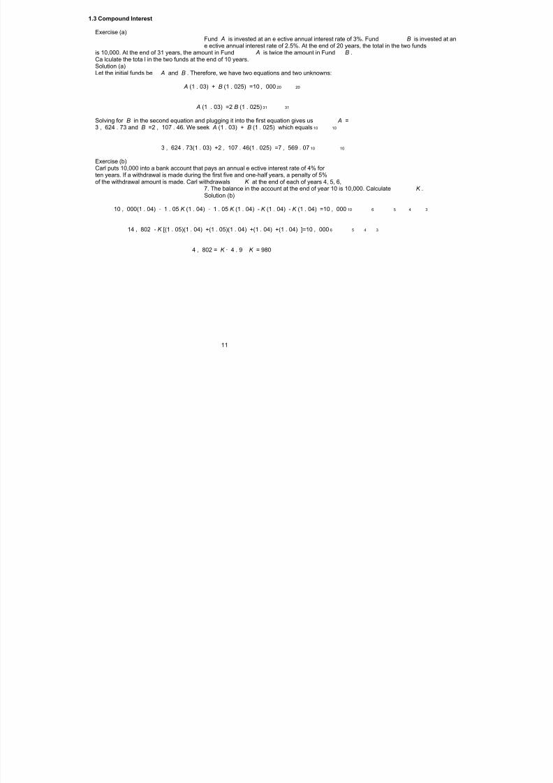
1.3 Compound Interest
Exercise (a)Fund A is invested at an e ective annual interest rate of 3%. Fund B is invested at ane ective annual interest rate of 2.5%. At the end of 20 years, the total in the two funds
is 10,000. At the end of 31 years, the amount in Fund A is twice the amount in Fund B .Ca lculate the tota l in the two funds at the end of 10 years.Solution (a)Let the initial funds be A and B . Therefore, we have two equations and two unknowns:
A (1 . 03) + B (1 . 025) =10 , 000 20 20
A (1 . 03) =2 B (1 . 025) 31 31
Solving for B in the second equation and plugging it into the first equation gives us A =3 , 624 . 73 and B =2 , 107 . 46. We seek A (1 . 03) + B (1 . 025) which equals 10 10
3 , 624 . 73(1 . 03) +2 , 107 . 46(1 . 025) =7 , 569 . 07 10 10
Exercise (b)Carl puts 10,000 into a bank account that pays an annual e ective interest rate of 4% for ten years. If a withdrawal is made during the first five and one-half years, a penalty of 5%of the withdrawal amount is made. Carl withdrawals K at the end of each of years 4, 5, 6,
7. The balance in the account at the end of year 10 is 10,000. Calculate K .Solution (b)
10 , 000(1 . 04) - 1 . 05 K (1 . 04) - 1 . 05 K (1 . 04) - K (1 . 04) - K (1 . 04) =10 , 000 10 6 5 4 3
14 , 802 - K [(1 . 05)(1 . 04) +(1 . 05)(1 . 04) +(1 . 04) +(1 . 04) ]=10 , 000 6 5 4 3
4 , 802 = K · 4 . 9 K = 980
11
8/8/2019 3500145 Financial Math for Actuary and Businessman
http://slidepdf.com/reader/full/3500145-financial-math-for-actuary-and-businessman 14/181
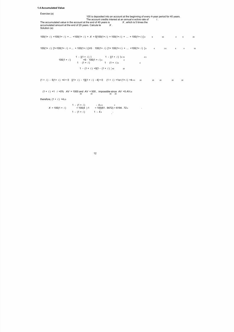
1.4 Accumulated Value
Exercise (a)100 is deposited into an account at the beginning of every 4-year period for 40 years.The account credits interest at an annual e ective rate of i .
The accumulated value in the account at the end of 40 years is X , which is 5 times theaccumulated amount at the end of 20 years. Calcula te X .Solution (a)
100(1+ i ) +100(1+ i ) + ... +100(1+ i ) = X = 5[100(1+ i ) + 100(1+ i ) + ... + 100(1+ i ) ] 4 8 40 4 8 20
100(1+ i ) [1+100(1+ i ) + ... + 100(1+ i ) ]=5 · 100(1+ i ) [1+ 100(1+ i ) + ... +100(1+ i ) ] 4 4 3 6 4 4 16
1 - [(1 + i ) ] 1 - [(1 + i ) ] 4 10 4 5100(1 + i ) =5 · 100(1 + i ) 4 4
1 - (1 + i ) 1 - (1 + i ) 4 4
1 - (1 + i ) =5[1 - (1 + i ) ] 40 20
(1 + i ) - 5(1+ i ) +4 = 0 [(1+ i ) - 1][(1 + i ) - 4] = 0 (1 + i ) =1or (1+ i ) =4 4 0 20 20 20 20 20
(1 + i ) =1 i =0% AV = 1000 and AV = 500 , impossible since AV =5 AV 2040 20 40 20
therefore, (1 + i ) =4 20
1 - (1 + i ) - 4 4 0 2
X = 100(1 + i ) = 100(4 ) 1 = 100(61 . 9472) = 6194 . 72 4 1
5
1 - (1 + i ) 1 - 4 4 1
5
12

8/8/2019 3500145 Financial Math for Actuary and Businessman
http://slidepdf.com/reader/full/3500145-financial-math-for-actuary-and-businessman 15/181
1.5 Present Value
Exercise (a)Annual payments are made at the end of each year, forever. The payments at time n isdefined as n for the first n yea rs. After year n , the payments remain constant at n .The 3
2
present value of these payments at time 0 is 20 n when the annual e ective rate of interest 2
is 0% for the first n yea rs and 25% thereafter. Calculate n .Solution (a)
[(1 ) v +(2 ) v +(3 ) v + ... +( n ) v ]+ v [( n ) v +( n ) v +( n ) v + ... ]=20 n 3 3 2 3 3 3 n n 2 1 2 2 2 3 20% 0% 0% 0 % 0% 25% 25% 25%
[(1 )+(2 )+(3 )+ ... +( n )] + ( n ) v [1 + v + v + ... ]=20 n 3 3 3 3 2 1 2 225% 25% 25%
n ( n +1) 1 2 2n ) v =20 n 2 2
25 % 4 +( 1 - v 2 5%
( n +1) 2
. 8) 14 +( 1 - . 8 =20
( n +1) ( n +1) ( n +1) 2 2
n =74 +4=20 4 =16 2 =4
Exercise (b)At a n e ective annua l interest rate of i , i> 0, each of the following two sets of payments has
present value K :(i) A payment of 121 immediately and another payment of 121 at the end of one year.(ii) A payment of 144 at the end of two years and another payment of 144 at the end of threeyears.Calculate K .Solution (b)
121 + 121 v = 144 v + 144 v = K 2 3
121(1 + v ) = 144 v (1 + v ) v = 11 2
12
K = 121(1 + 11 K = 231 . 9212)
13
8/8/2019 3500145 Financial Math for Actuary and Businessman
http://slidepdf.com/reader/full/3500145-financial-math-for-actuary-and-businessman 16/181
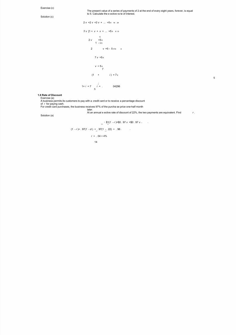
Exercise (c)The present value of a series of payments of 2 at the end of every eight years, forever, is equalto 5. Calculate the e ective ra te of interest.
Solution (c)
2 v +2 v +2 v + ... =5 8 16 24
2 v [1 + v + v + ... =5 8 8 1 6
12 v =5 8
1 - v 8
2 v =5 - 5 v 8 8
7 v =5 8
v = 5 8
7
(1 + i ) = 7 8
5
18
1+ i = 7 i = . 042965
1.6 Rate of DiscountExercise (a)A business permits its customers to pay with a credit card or to receive a percentage discountof r for paying cash.For credit card purchases, the business receives 97% of the purcha se price one-half month
later.At an annual e ective rate of discount of 22%, the two payments are equivalent. Find r .
Solution (a)
* $1(1 - r )=$0 . 97 v =$0 . 97 v 1 1 1
12 2 24
(1 - r )= . 97(1 - d ) = . 97(1 - . 22) = . 96 1 1
2 4 2 4
r = . 04 = 4%
14

8/8/2019 3500145 Financial Math for Actuary and Businessman
http://slidepdf.com/reader/full/3500145-financial-math-for-actuary-and-businessman 17/181
Exercise (b)You deposit 1,000 today and another 2,000 in five years into a fund that pays simple dis-counting at 5% per year.
Your friend makes the same deposits into another fund, but at time n and 2 n , respectively.This fund credits interest at an annual e ective rate of 10%.At the end of 10 years, the accumulated value of your deposits is exactly the same as theaccumulated value of your friend’s deposits.Calculate n .Solution (b)
1 , 000[1 - 5%(10)] +2 , 000[1 - 5%(5)] =1 , 000(1 . 10) +2 , 000(1 . 10) - 1 - 1 1 0 - n 10 - 2 n
1 , 000 , 000, 000(1 . 10) v +2 , 000(1 . 10) v 1 0 n 10 2 n
. 5 + 2 . 75 =1
4 , 666 . 67 = 2 , 593 . 74 v +5 , 187 . 48 v 5 , 187 . 48 v +2 , 593 . 74 v - 4 , 666 . 67 =0 n 2 n 2 n n
a b c
- 2 , 593 . 74 + 2 , 593 . 74 - 4(5 , 187 . 48)( - 4 , 666 . 67) 2
v = . 7306 n
2(5 , 187 . 48) =
ln (1 .36824)
n (1 . 10) = 1 . 36824 n = . 29. 7306 =1 ln (1 . 10) =3
Exercise (c)A deposit of X is made into a fund which pays an annual e ective interest rate of 6% for 10years.At the same time , X/2 is deposited into another fund which pays an annual e ective rate of
discount of d for 10 years.The amounts of interest earned over the 10 years are equal for both funds.
Calculate d .Solution (c)
X
10 - 10 X (1 . 06) - X = - d ) - X 2 (1 2
d =0 . 0905
15

8/8/2019 3500145 Financial Math for Actuary and Businessman
http://slidepdf.com/reader/full/3500145-financial-math-for-actuary-and-businessman 18/181
1.7 Constant Force of InterestExercise (a)
You are give n that AV = Kt + Lt + M ,for0 = t = 2, and that AV = 100, AV = 110, 2t 0 1
and AV = 136. Determine the force of interest at time t = . 12 2
Solution (a)
AV = M = 1000
AV = K + L + M = 110 K + L =101
AV =4 K +2 L + M = 136 4 K +2 L =362
These equations solve for K =8, L =2, M = 100.We know th at
AV d Kt + Lt d = = 2 dt
t AV Kt + Lt + M 2t
)+2 1
d = (2)(8)( . 09709 2
(8)( ) +(2)( ) + 100 = 10 103 =0 1 1 1 22
2 2
Exercise (b)Fund A accumulates at a simple interest rate of 10%. Fund B accumulates at a simple
discount rate of 5%. Find the point in time at which the forces of interest on the two fundsare equal.
Solution (b)
AV F =1+ . 10 t and AV F =(1+ . 05 t ) A B - 1t t
AV F . 10 d A
t d = = A dt
t AV F 1+ . 10 t A
t
AV F . 05(1 - . 05 t ) d B - 2
t d = = = . 05(1 - . 05 t ) B dt - 1
t AV F 1 - . 05 t ) B - 1t
Equating and solve for t
. 10 . 05= 10 - . 005 t = . 05 + . 005 t t =5
1+ . 10 t 1 - . 05 t .
16

8/8/2019 3500145 Financial Math for Actuary and Businessman
http://slidepdf.com/reader/full/3500145-financial-math-for-actuary-and-businessman 19/181
1.8 Varying Force of InterestExercise (a)
On 15 March 2003, a student deposits X into a bank account. The account is credited withsimple interest where i =7.5%On the same date, the student’s professor deposits X into a di erent bank acco unt where
interest is credited at a force of interest
t d = 2 0 .
t t + k ,t= 2
From the end of the fourth year until the end of the eighth year, both accounts earn the samedollar amount of interest.Calculate k .Solution (a)
Simple Interest Earned = AV -AV = X [1+ . 075(8)] -X [1+ . 075(4)] = X (0 . 075)(4) = X ( . 3)8 4
8 4
d · dt d · dt t t
Compound Interest Earned = AV - AV = Xe - Xe0 0 8 4
8 4 2 t 2 t f ( t ) f ( t ) 8 4
· dt · dt (8) (4) f ( t ) f ( t ) t + k · dt t + k · dt 2 2 Xe - Xe = Xe-Xe = X f -X f
0 0 0 0
f (0) f (0)
(8) + k (4) + k 48 2 2
X = X co mpound interest(0) + k - X (0) + k k , 2 2
48 X ( . 3) = X 3=48 30 k =48 k = 160
k . k .
17

8/8/2019 3500145 Financial Math for Actuary and Businessman
http://slidepdf.com/reader/full/3500145-financial-math-for-actuary-and-businessman 20/181
Exercise (b)
Payments are made to an account at a continuous rate of , k +8 tk +( tk ) ,where0 = t = 10 2 2 2
and k> 0.Interest is credited at a force of interest where
t d = 8+2t 1+8 t + t 2
After 1 0 years, the account is worth 88 , 690.Calculate k .Solution (b)
10
[ k +8 tk +( tk ) ](1 + i ) dt =88 , 690 2 2 2 10 -t
0
10 8+2 s f ( s ) 10 10
· ds d · ds · ds f (10) s f ( s ) 1+8 s + s 2 (1 +i ) = e = e = e = 10 - t t t t
f ( t )
2
= 1 + 8(10) + (10) = 1811+8 t + t 1+8 t + t 2 2
1 0
[ k +8 tk + ( tk ) ] 181 dt =88 , 690 2 2 2
1+8 t + t 20
10
k [1 + 8 t + t ] 181 dt =88 , 690 k (181)(10) = 88 , 690 k =49 k =7 2 2 2 2
1+8 t + t 20
18

8/8/2019 3500145 Financial Math for Actuary and Businessman
http://slidepdf.com/reader/full/3500145-financial-math-for-actuary-and-businessman 21/181
Exercise (c). 05
Fund A accumulates at a constant force of interest of d = at time t ,for t = 0, and A
1+ . 05 t t Fund B accumulates a t a constant force of interest of d =5%. Youaregiven: B
(i) The amount in Fund A at time zero is 1,000.(ii) The amount in Fund B at time zero is 500.
(iii) The amount in Fund C at any time t , t = 0, is equal to the sum of the amounts in Fund A and Fund B . Fund C accumulates at a force of interest of d ,for t 0. C
t
Calculate d . C
2
Solution (c)
t
d dt s
AV = AV + AV =1 , 000 e + 500 e C A B . 05 t
0t t t
t . 05
f ( t ) 1+ . 05 s · dsC . 05 t . 05 t AV =1 , 000 e + 500 e =1 , 000 e
0
f (0) + 500 t
. 05( t ) AV =1 , 000 1+ . 05) e = 1000[1 + . 05 t ] + 500 e C . 05 t . 05 t
t 1+ . 05(0) + 500(
d C . 05 t . 0 5 t =1 , 000( . 05) + 500( . 05) e =50+25
dt AV t
AV d e C . 05 t
t
d = = 50 + 25dt
t 1000[1+ . 05 t ] + 500 e AV C . 05 t
t
e . 05(2)
d = 50 + 25 =4 . 697%2 1 , 000[1 + . 05(2)] + 500 e . 05(2)
19

8/8/2019 3500145 Financial Math for Actuary and Businessman
http://slidepdf.com/reader/full/3500145-financial-math-for-actuary-and-businessman 22/181
Exercise (d)t
Fund F accumulates at the rate d = 1 . Fund G accumulates at the rate d = 4 .t t 1+ t 1+2 t 2
F ( t ) is the amount in Fund F at time t, and G ( t ) is the amount in fund G at time t, withF (0) = G (0). Let H ( t )= F ( t ) - G ( t ). Calculate T , the value of time t when H ( t )isamaximum.Solution (d)
Since F (0) = G (0), we can assume an initial deposit of 1. Then we have,
1 t
1+ r · dr F ( t )= e = e =1+ t ln (1 + t ) -ln ( 1 )0
4 r t
dr 1+2 r 2 G ( t )= e = e =1+2 t l n (1 +2 t 2 ) -l n (1 ) 2
0
d H ( t )= t - 2 t and ( t )=1 - 4 t =0 t = 1 2
dt H 4
20

8/8/2019 3500145 Financial Math for Actuary and Businessman
http://slidepdf.com/reader/full/3500145-financial-math-for-actuary-and-businessman 23/181
2 Level AnnuitiesOverview
Definition of An Annuity – a series of payments made at equal intervals of time (annually or otherwise) – payments made for certain over a fixed perio d of time are called an a nnuity-certain – payments made for an uncertain period of time are called a contingent annuity – the payment frequency and the interest conversion period are equal – the payments are level
2.1 Annuity-ImmediateDefinition
– payments of 1 are made at the end of every year for n years
...1 1 1 1
...0 1 2 n - 1 n
Annuity-Immediate Present Value Factor – the present value (at t = 0) of an annuity–immediate, where the annual e ective rate of
interest is i , shall be denoted as a and is calculated as follows:n
i
2 n - 1 n a =(1) v +(1) v + ··· +(1) v +(1) v n
i
= v (1 + v + v + ··· + v + v ) 2 n - 2 n - 1
1 - v n= 1
1+ i 1 - v
1 - v n= 1
1+ i d 1 - v n
= 11+ i i
1+ i
- v n= 1
i
21

8/8/2019 3500145 Financial Math for Actuary and Businessman
http://slidepdf.com/reader/full/3500145-financial-math-for-actuary-and-businessman 24/181
Annuity-Immediate Accumulated Value Factor – the accumulated value (at t = n ) of an annuity–immediate, where the annual e ective rate
of interest is i , shall be denoted as s and is calculated as follows:n
i
s = 1 + (1)(1 + i )+ ··· + (1)(1 + i ) + (1)(1 + i ) n - 2 n - 1n
i
- (1 + i ) n
= 11 - (1 + i )
- (1 + i ) n
= 1-i i ) - 1 n
= (1 +i
Basic Relationship 1:1= i · a + v n n
Consider an n –year investment where 1 is invested a t time 0.
The present value of this single payment income stream at t =0is1.
Alternatively, consider a n –year investment where 1 is invested at time 0 and pro ducesannual interest payments of (1) · i at the end of each year and then the 1 is refunded at t = n .
1+
...i i i i
...
0 1 2 n - 1 n
The present value of this multiple payment income stream at t =0 is i · a +(1) v . n
n
Theref ore, the present value of both investment opportunities a re equal.- v n
Also note that a = 1 1= i · a + v . n
n n i
22

8/8/2019 3500145 Financial Math for Actuary and Businessman
http://slidepdf.com/reader/full/3500145-financial-math-for-actuary-and-businessman 25/181
Basic Relationship 2: PV (1 + i ) = FV and PV = FV · v n n
– if the future value at time n , s , is discounted back to time 0, then you will have itsn
present value, an
i ) - 1 n
s · v = (1 + n n
n i · v i ) · v - v n n n
= (1 +i
- v n= 1
i = a
n
– if the present value at time 0, a , is accumulated fo rward to time n , then you will havenits future value, s
n
- v na · (1 + i ) = 1 (1 + i ) n n
n i i ) - v (1 + i ) n n n
= (1 +i
i ) - 1 n
= (1 +i
= sn
23

8/8/2019 3500145 Financial Math for Actuary and Businessman
http://slidepdf.com/reader/full/3500145-financial-math-for-actuary-and-businessman 26/181
Basic Relationship 3: 1 = 1 + i a s
n n
Consider a loan of 1, to be paid back over n years with equal annual payments of P madeat the end of each year. An annual e ective rate of interest, i , is used. The present value o f this single payment loan must be equal to the present value of the multiple payment incomestream.
P · a =1n
i
P = 1a
ni
Alternatively, consider a loan of 1, where the annual interest due on the loan, (1) i ,ispaidatthe end of each year for n years and the loan amount is paid back at time n .
In order to produce the loan amount at time n , annual payments at the end of each year,for n years, will be made into an account that credits interest at an annual e ective rate of interest i .
The future value of the multiple deposit inco me stream must equal the future value of thesingle payment, which is the loan of 1.
D · s =1n
i
D = 1s
ni
The total annual payment will be the interest payment and account payment:
i + 1s
ni
Therefore, a level annual annuity payment on a loan is the same as making an annual in-terest payment each year plus making annual deposits in order to save for the loa n repayment.
Also note that1 i (1 + i ) i (1 + i ) n n
= × =a 1 - v (1 + i ) (1 + i ) - 1 n n n
ni
i (1 + i ) + i - i i [(1 + i ) - 1] + i n n
=(1 + i ) - 1 = (1 + i ) - 1 n n
i = i + i + 1
(1 + i ) - 1 = s n
n
24

8/8/2019 3500145 Financial Math for Actuary and Businessman
http://slidepdf.com/reader/full/3500145-financial-math-for-actuary-and-businessman 27/181
2.2 Annuity–DueDefinition
– payments of 1 are made at the beginning of every year for n years
...1 1 1 1
...0 1 2 n - 1 n
Annuity-Due Present Value Factor – the present value (at t = 0) of an annuity–due, where the annual e ective rate of interest isi , shall be denoted as ¨ a and is calculated as follows:
ni
2 n - 2 n - 1 ¨ a =1+(1) v +(1) v + ··· +(1) v +(1) v n
i
- v n= 1
1 - v - v n
= 1d
Annuity-Due Accumulated Value Factor – the accumulated value (at t = n ) of an annuity–due, where the annual e ective rate of interest
is i , shall be denoted as ¨ s and is calculated as follows:n
i
¨ s = (1)(1 + i ) + (1)(1 + i ) + ··· + (1)(1 + i ) + (1)(1 + i ) 2 n - 1 n
ni
=(1+ i )[1 + (1 + i )+ ··· +(1+ i ) +(1+ i ) ] n - 2 n - 1
- (1 + i ) n
=(1+ i ) 11 - (1 + i )
- (1 + i ) n
=(1+ i ) 1-i i ) - 1 n
=(1+ i ) (1 +i
i ) - 1 n
= (1 +d
25

8/8/2019 3500145 Financial Math for Actuary and Businessman
http://slidepdf.com/reader/full/3500145-financial-math-for-actuary-and-businessman 28/181
Basic Relationship 1:1= d · ¨ a + v nn
Consider an n –year investment where 1 is invested a t time 0.
The present value of this single payment income stream at t =0is1.
Alternatively, consider a n –year investment where 1 is invested at time 0 and produces annualinterest payments of (1) ·d at the beginning of each year and then have the 1 refunded at t = n .
1
d d d d ...
...0 1 2 n - 1 n
The present value of this multiple payment income stream at t =0 is d · ¨ a +(1) v . n
n
Theref ore, the present value of both investment opportunities a re equal.- v n
Also note that ¨ a = 1 1= d · ¨ a + v . n
n n d
Basic Relationship 2: PV (1 + i ) = FV and PV = FV · v n n
– if the future value at time n ,¨ s , is discounted back to time 0, then you will have itsn
present value, ¨ an
i ) - 1 i ) · v - v - v n n n n n
s ¨ · v = (1 + = (1 + = 1 =¨ a n n
n n d · v d d
– if the present value at time 0, ¨ a , is accumulated fo rward to time n , then you will haven
its future value, ¨ sn
- v i ) - v (1 + i ) i ) - 1 n n n n n
¨ a · (1 + i ) = 1 (1 + i ) = (1 + = (1 + =¨ s n n
n n d d d
26

8/8/2019 3500145 Financial Math for Actuary and Businessman
http://slidepdf.com/reader/full/3500145-financial-math-for-actuary-and-businessman 29/181
Basic Relationship 3: 1 = 1 + d ¨ a s ¨
n n
Consider a loan of 1, to be paid back over n years with equal annual payments of P madeat the beginning of each year. An annual e ective rate of interest, i , is used. The presentvalue of the single payment loan must be equal to the present value of the multiple paymentstream.
P · a ¨ =1n
i
P = 1¨ a
ni
Alternatively, consider a loan of 1, where the annual interest due on the loan, (1) · d ,ispaidat the beginning of each year for n years and the loan amount is paid back at time n .
In order to produce the loan amount at time n , annual payments at the beginning of eachyear, for n years, will be made into an account that credits interest at an annual e ectiverate of interest i .
The future value of the multiple deposit inco me stream must equal the future value of thesingle payment, which is the loan of 1.
D · ¨ s =1n
i
D = 1s ¨
ni
The total annual payment will be the interest payment and account payment:
d + 1¨ s
ni
Theref ore, a level annual annuity payment is the same as making an annual interest paymenteach year and making annual deposits in order to save for the loan repayment.
Also note that1 d (1 + i ) d (1 + i ) n n
= × =¨ a 1 - v (1 + i ) (1 + i ) - 1 n n n
ni
d (1 + i ) + d - d d [(1 + i ) - 1] + d n n
=(1 + i ) - 1 = (1 + i ) - 1 n n
d = d + d + 1
(1 + i ) - 1 = ¨ s n
n
Basic Relationship 4 :AnnuityDue = Annuity Immediate × (1 + i )- v - v n n
¨ a = 1 = 1 (1 + i )= a · (1 + i )n n d i ·
i ) - 1 i ) - 1 n n
s ¨ = (1 + = (1 + (1 + i )= s · (1 + i )n n d i ·
An annuity–due starts one period earlier than an annuity-immediate and as a result, earnsone more perio d o f interest, hence it will be larger.
27

8/8/2019 3500145 Financial Math for Actuary and Businessman
http://slidepdf.com/reader/full/3500145-financial-math-for-actuary-and-businessman 30/181
Basic Relationship 5:¨ a =1+ an n - 1
¨ a =1+[ v + v + ··· + v + v ] 2 n - 2 n - 1n
=1+ v [1 + v + ··· + v + v ] n - 3 n - 2
1 - v n - 1
=1+ v 1 - v
1 - v n - 1
=1+ 11+ i d
1 - v n - 1
=1+ 11+ i i/ 1+ i - v n - 1
=1+1i
=1+ a
n - 1This relationship can be visualized with a time line diagram.
1
a +
...1 1 1
n-1
...0 1 2 n - 1 n
An additional payment of 1 at time 0 results in a becoming n payments that now com-n - 1
mence at the beginning of each year which is ¨ a .n
28
8/8/2019 3500145 Financial Math for Actuary and Businessman
http://slidepdf.com/reader/full/3500145-financial-math-for-actuary-and-businessman 31/181
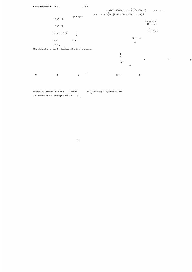
Basic Relationship 6: s =1+¨ sn n - 1
s =1+[(1+ i )+(1+ i ) + ··· +(1+ i ) +(1+ i ) ] 2 n - 2 n - 1n
n - 3 n - 2 =1+(1+ i )[1 + (1 + i )+ ··· +(1+ i ) +(1+ i ) ]- (1 + i ) n - 1
=1+(1+ i ) 11 - (1 + i )- (1 + i ) n - 1
=1+(1+ i ) 1-i i ) - 1 n - 1
=1+(1+ i ) (1 +i
i ) - 1 n - 1
=1+ (1 +d
=1+¨ s
n - 1This relationship can also the visualized with a time line diagram.
1+
.. ... s 1 11
n-1
...0 1 2 n - 1 n
An additional payment of 1 at time n results in ¨ s becoming n payments that nown - 1
commerce at the end of each year which is sn
29

8/8/2019 3500145 Financial Math for Actuary and Businessman
http://slidepdf.com/reader/full/3500145-financial-math-for-actuary-and-businessman 32/181
2.3 Deferred Annuities – There are three alternative dates to valuing annuities rather than at the beginning of the
term ( t =0)orattheendoftheterm( t = n )(i) present values more than one period before the first payment date
(ii) accumulated values more than one period after the last payment date(iii) current value between the first and last payment dates
– The following example will be used to illustrate the above cases. Consider a series of paymentsof 1 that are made at time t =3to t =9,inclusive.
1 1 1 1 1 1 1
0 1 2 3 4 5 6 7 8 9 10 11 12
Present Values More than One Period Before The First Payment DateAt t = 2, there exists 7 future end-of-year payments whose present value is represented bya . If this value is discounted back to time t = 0, then the value of this series of payments
7
(2 perio ds before the first end-of-year payment) is
a = v · a . 22 | 7 7
The general form is:
a = v · a . m
n n m|i i
Alternatively, at t = 3, there exists 7 future beginning-of-year payments whose present valueis represented by ¨ a . If this va lue is discounted back to time t = 0, then the value of this
7
series of payments (3 periods before the first beginning-of-year payment) is
¨ a = v · ¨ a . 33 | 7 7
The general form is:
¨ a = v · ¨ a . m
m| n ni
Another way to examine this situation is to pretend that there are 9 end-of-year payments.This can be done by adding 2 more payments to the existing 7. In this case, let the 2 addi-tional payments be made at t = 1 and 2 and be denoted as 1 .
30

8/8/2019 3500145 Financial Math for Actuary and Businessman
http://slidepdf.com/reader/full/3500145-financial-math-for-actuary-and-businessman 33/181
1 1 1 1 1 1 1 1 1
0 1 2 3 4 5 6 7 8 9 10 11 12
At t = 0, there now exists 9 end-of-year payments whose present value is a .Thispresent
9
value of 9 payments would then be reduced by the present value of the two imaginary pay-ments, represented by a . Therefore, the present value at t =0is
2
a - a ,9 2
and this results in
v · a = a - a . 27 9 2
The general form is
v · a = a - a . m
n m m + n
31

8/8/2019 3500145 Financial Math for Actuary and Businessman
http://slidepdf.com/reader/full/3500145-financial-math-for-actuary-and-businessman 34/181
With the annuity–due version, one can pretend that there are 10 payments being made.
This can be done by adding 3 payments to the existing 7 payments. In this case, let the 3additional payments be made at t = 0, 1 and 2 and be denoted as 1 .
1 1 1 1 1 1 1 1 1 1
0 1 2 3 4 5 6 7 8 9 10 11 12
At t = 0, there now exists 10 beginning-of-year payments whose present value is ̈ a .This1 0
present value of 10 payments would then be reduced by the present value of the three ima g-inary payments, represented by ¨ a . Therefo re, the present value at t =0is
3
¨ a - ¨ a ,10 3
and this results in
v · ¨ a =¨ a - ¨ a . 37 1 0 3
The general form is
m v · ¨ a =¨ a - ¨ a .n m m + n
Accumulated Values More Than One Period After The Last Payment DateAt t = 9, there exists 7 past end-of-year payments whose accumulated value is representedby s . If this value is accumulated forward to time t = 12, then the value of this series of
7
payments (3 periods after the last end-o f- year payment) is
s · (1 + i ) . 37
Alternatively, at t = 10 , there exists 7 past beginning-of-year payments whose accumulatedvalue is represented by ¨ s . If this value is accumulated forwa rd to time t = 12, then the
7
value of this series of payments (2 periods after the last beginning-of-year payment) is
¨ s · (1 + i ) . 27
Another way to examine this situation is to pretend that there are 10 end- of-year payments.This can be done by adding 3 more payments to the existing 7. In this case, let the 3 addi-tional payments be made at t = 10, 11 and 12 and be denoted as 1 .
32

8/8/2019 3500145 Financial Math for Actuary and Businessman
http://slidepdf.com/reader/full/3500145-financial-math-for-actuary-and-businessman 35/181
1 1 1 1 1 1 1 1 1 1
0 1 2 3 4 5 6 7 8 9 10 11 12
At t = 12, there now exists 10 end-of-year payments who se present value is s . This future
10
value of 10 payments would then be reduced by the future value of the three ima ginarypayments, represented by s . Therefore, the accumulated value at t =12is
3
s - s ,10 3
and this results in
s · (1 + i ) = s - s . 37 10 3
The general form is
s · (1 + i ) = s - s . m
n m m + n
With the annuity–due version, one can pretend that there are 9 payments being made. Thiscan be done by adding 2 payments to the existing 7 payments. In this case, let the 2 addi-tional payments be made at t = 10 and 11 and be denoted as 1 .
33

8/8/2019 3500145 Financial Math for Actuary and Businessman
http://slidepdf.com/reader/full/3500145-financial-math-for-actuary-and-businessman 36/181
1 1 1 1 1 1 1 1 1
0 1 2 3 4 5 6 7 8 9 10 11 12
At t = 12, there now exists 9 beginning-of-year payments whose accumulated value is ¨ s .
9
This future value of 9 payments would then be reduced by the future value of the twoimaginary payments, represented by ¨ s . Therefore, the accumulated value at t =12is
2
¨ s - s ¨ ,9 2
and this results in
¨ s · (1 + i ) =¨ s - ¨ s . 27 9 2
The general form is
¨ s · (1 + i ) =¨ s - s ¨ . m
n m m + n
34
8/8/2019 3500145 Financial Math for Actuary and Businessman
http://slidepdf.com/reader/full/3500145-financial-math-for-actuary-and-businessman 37/181
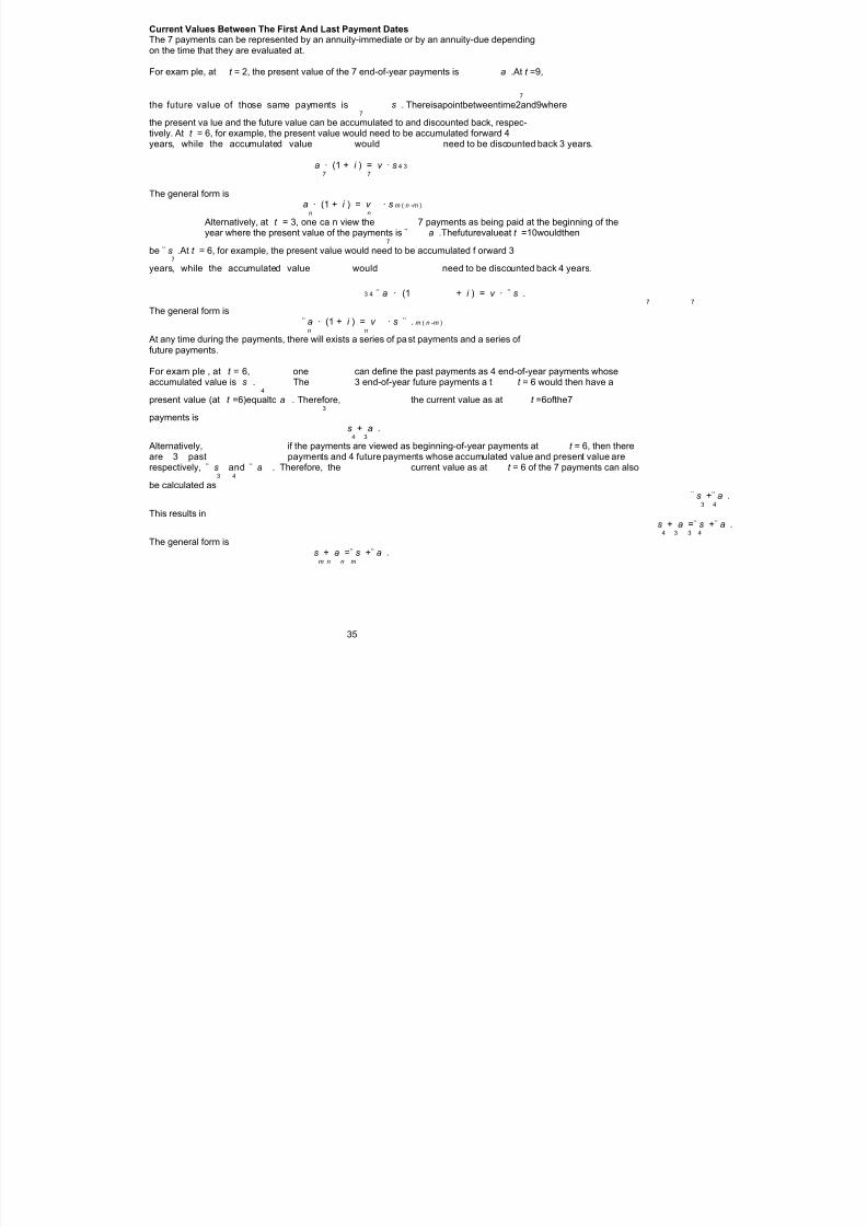
Current Values Between The First And Last Payment DatesThe 7 payments can be represented by an annuity-immediate or by an annuity-due dependingon the time that they are evaluated at.
For exam ple, at t = 2, the present value of the 7 end-of-year payments is a .At t =9,
7
the future value of those same payments is s . Thereisapointbetweentime2and9where7
the present va lue and the future value can be accumulated to and discounted back, respec-tively. At t = 6, for example, the present value would need to be accumulated forward 4years, while the accumulated value would need to be discounted back 3 years.
a · (1 + i ) = v · s 4 37 7
The general form isa · (1 + i ) = v · s m ( n -m )
n nAlternatively, at t = 3, one ca n view the 7 payments as being paid at the beginning of theyear where the present value of the payments is ¨ a .Thefuturevalueat t =10wouldthen
7
be ¨ s .At t = 6, for example, the present value would need to be accumulated f orward 37
years, while the accumulated value would need to be discounted back 4 years.
3 4 ¨ a · (1 + i ) = v · ¨ s .7 7
The general form is¨ a · (1 + i ) = v · s ¨ . m ( n -m )
n n
At any time during the payments, there will exists a series of past payments and a series of future payments.
For exam ple , at t = 6, one can define the past payments as 4 end-of-year payments whoseaccumulated value is s . The 3 end-of-year future payments a t t = 6 would then have a
4
present value (at t =6)equalto a . Therefore, the current value as at t =6ofthe73
payments is
s + a .4 3
Alternatively, if the payments are viewed as beginning-of-year payments at t = 6, then thereare 3 past payments and 4 future payments whose accumulated value and present value arerespectively, ¨ s and ¨ a . Therefore, the current value as at t = 6 of the 7 payments can also
3 4
be calculated as¨ s +¨ a .
3 4
This results ins + a =¨ s +¨ a .
4 3 3 4
The general form iss + a =¨ s +¨ a .
m n n m
35
8/8/2019 3500145 Financial Math for Actuary and Businessman
http://slidepdf.com/reader/full/3500145-financial-math-for-actuary-and-businessman 38/181
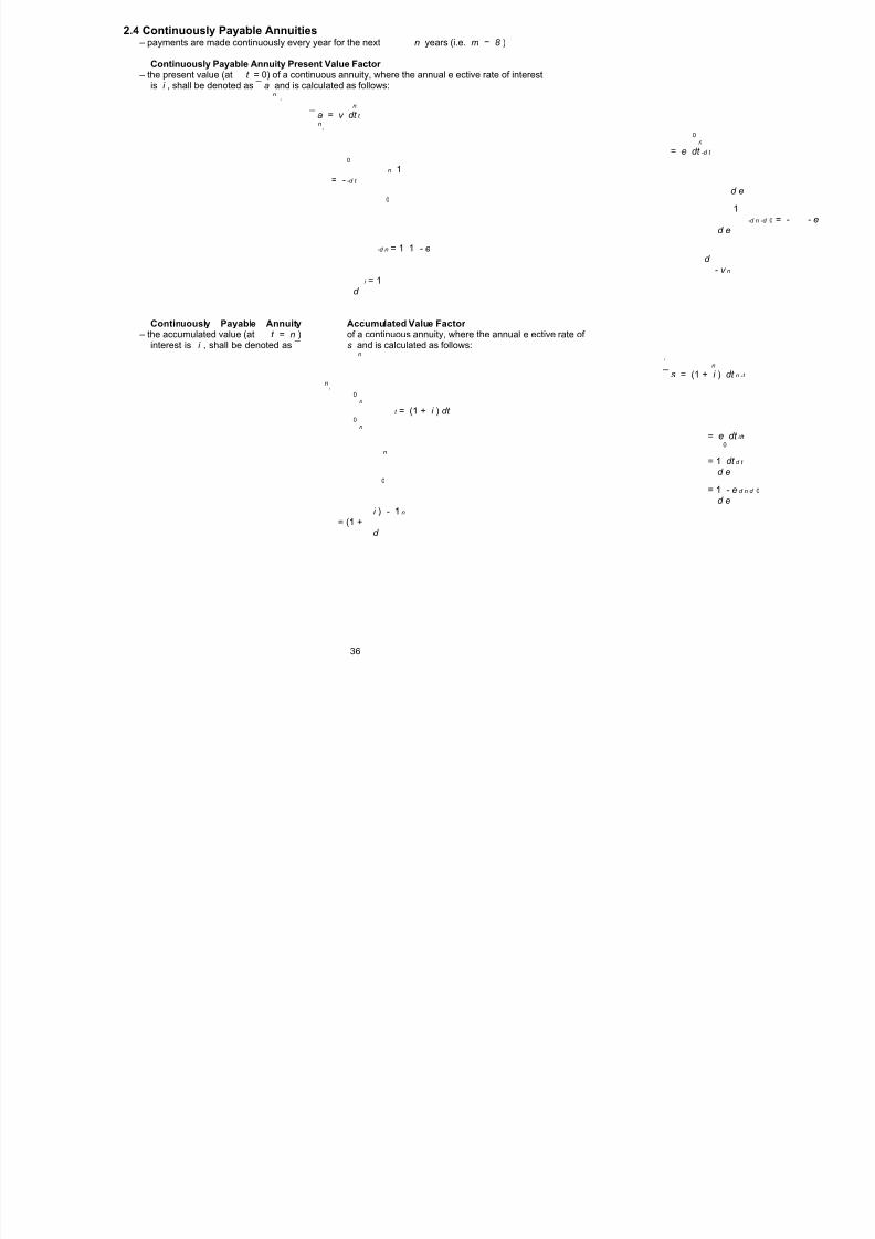
2.4 Continuously Payable Annuities – payments are made continuously every year for the next n years (i.e. m = 8 )
Continuously Payable Annuity Present Value Factor – the present value (at t = 0) of a continuous annuity, where the annual e ective rate of interest
is i , shall be denoted as ¯ a and is calculated as follows:n
i
n
¯ a = v dt t n
i
0n
= e dt -d t
0
n 1= - -d t
d e0
1-d n -d 0 = - - e
d e
-d n = 1 1 - ed
- v ni = 1
d
Continuously Payable Annuity Accumulated Value Factor – the accumulated value (at t = n ) of a continuous annuity, where the annual e ective rate of
interest is i , shall be denoted as ¯ s and is calculated as follows:n
i
n
¯ s = (1 + i ) dt n -t
ni
0n
t = (1 + i ) dt 0
n
= e dt dt
0n
= 1 dt d t
d e0
= 1 - e d n d 0
d ei ) - 1 n
= (1 +d
36

8/8/2019 3500145 Financial Math for Actuary and Businessman
http://slidepdf.com/reader/full/3500145-financial-math-for-actuary-and-businessman 39/181
Basic Relationship 1:1= d · ¯ a + v nn
Basic Relationship 2: PV (1 + i ) = FV and PV = FV · v n n
– if the future value at time n ,¯ s , is discounted back to time 0, then you will have itsn
present value, ¯ an
i ) - 1 n
¯ s · v = (1 + n n
n d · v i ) · v - v n n n
= (1 +d
- v n= 1
d =¯ a
n
– if the present value at time 0, ̄ a , is accumulated fo rward to time n , then you will haven
its future value, ¯ sn
- v n¯ a · (1 + i ) = 1 (1 + i ) n n
n d i ) - v (1 + i ) n n n
= (1 +d
i ) - 1 n
= (1 +d
=¯ sn
37

8/8/2019 3500145 Financial Math for Actuary and Businessman
http://slidepdf.com/reader/full/3500145-financial-math-for-actuary-and-businessman 40/181
Basic Relationship 3: 1 = 1 + d ¯ a s ¯
n n
– Consider a loan of 1, to be paid back over n years with annual payments of P that arepaid continuously each year, for the next n yea rs. An annual e ective rate of interest,i , and annual force of interest, d , is used. The present value of this single payment loanmust be equal to the present value o f the multiple payment income stream.
P · ¯ a =1n
i
P = 1a ¯
ni
– Alternatively, consider a loan of 1, where the annual interest due on the loan, (1) × d ,ispaid continuously during the year for n years and the loan amount is paid back at timen .
– In order to produce the loan amount at time n , annual payments of D are paid continu-ously each year, for the next n years, into an account that credits interest at an annualforce of interest, d .
– The future value of the multiple deposit income stream must equal the future value of the single payment, which is the loan of 1.
D · ¯ s =1n
i
D = 1s ¯
ni
– The total annual payment will be the interest payment and account payment:
d + 1 ¯ s
ni
–Notethat1 d (1 + i ) d (1 + i ) n n
= × = ¯ a 1 - v (1 + i ) (1 + i ) - 1 n n n
ni
d (1 + i ) + d - d d [(1 + i ) - 1] + d n n
=(1 + i ) - 1 = (1 + i ) - 1 n n
d = d + d + 1
(1 + i ) - 1 = s ¯ nn
– Therefore, a level continuous annua l annuity payment on a loan is the same as makingan annual continuous interest payment each year plus making level annual continuousdeposits in order to save for the loan repayment.
38

8/8/2019 3500145 Financial Math for Actuary and Businessman
http://slidepdf.com/reader/full/3500145-financial-math-for-actuary-and-businessman 41/181
i i Basic Relationship 4:¯ a = , ¯ s =
n n n n d · a d · s – Consider annual payments of 1 made continuously each year for the next n years. Over
a one-year period, the continuous payments will accumulate at the end of the year toa lump sum of ¯ s . If this end-of-year lump sum exists for each year of the n -year
1
annuity- immediate, then the present value (at t = 0) of these end-of-year lump sums isthe same as ¯ a :
n
¯ a =¯ s · an n 1
i =
n d · a
– Therefo re, the accumulated value (at t = n ) of these end-of-year lump sums is the sameas ¯ s :
n
s ¯ =¯ s · sn n 1
i =
n d · sd d
Basic Relationship 5:¯ a = ¨ a , ¯ s = s ¨n n n n d · d ·
– The mathematical development of this relationship is derived as follows:
- v - v n n
¨ a · d = 1 = 1 =¯ an n d d · d d d
i ) - 1 i ) - 1 n n
s ¨ · d = (1 + = (1 + =¯ sn n d d · d d d
39
8/8/2019 3500145 Financial Math for Actuary and Businessman
http://slidepdf.com/reader/full/3500145-financial-math-for-actuary-and-businessman 42/181
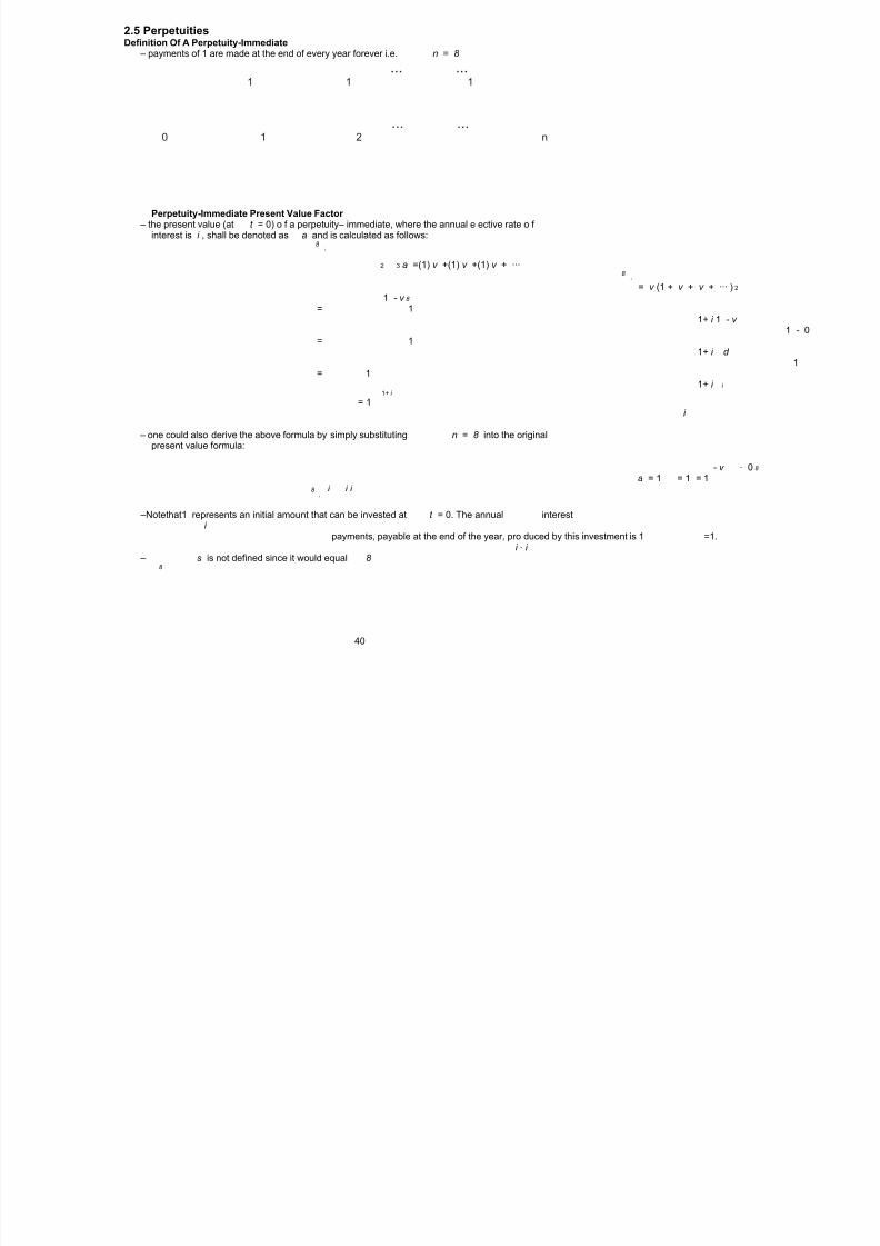
2.5 PerpetuitiesDefinition Of A Perpetuity-Immediate
– payments of 1 are made at the end of every year forever i.e. n = 8
... ...1 1 1
... ...0 1 2 n
Perpetuity-Immediate Present Value Factor – the present value (at t = 0) o f a perpetuity– immediate, where the annual e ective rate o f interest is i , shall be denoted as a and is calculated as follows:
8 i
2 3 a =(1) v +(1) v +(1) v + ···8
i
= v (1 + v + v + ··· ) 2
1 - v 8
= 11+ i 1 - v
1 - 0= 1
1+ i d 1
= 11+ i i
1+ i
= 1i
– one could also derive the above formula by simply substituting n = 8 into the originalpresent value formula:
- v - 0 8
a = 1 = 1 = 18 i i i
i
–Notethat1 represents an initial amount that can be invested at t = 0. The annual interesti
payments, payable at the end of the year, pro duced by this investment is 1 =1.i · i
– s is not defined since it would equal 8 8
40

8/8/2019 3500145 Financial Math for Actuary and Businessman
http://slidepdf.com/reader/full/3500145-financial-math-for-actuary-and-businessman 43/181
Basic Relationship 1: a = a - v · an 8 n 8
The present value formula for an annuity-immediate can be expressed as the di erence be-tween two perpetuity-immediates:
- v 1 n n
n n a = 1 = 1 = 1 · = a - v · a . n 8 8 i i - v i i - v i In this case, a perpetuity-immediate that is payable forever is reduced by perpetuity-immediatepayments that start after n years. The present value of both of these income streams, at t = 0, results in end-of-year payments remaining only for the first n years.
41

8/8/2019 3500145 Financial Math for Actuary and Businessman
http://slidepdf.com/reader/full/3500145-financial-math-for-actuary-and-businessman 44/181
Definition Of A Perpetuity-Due – payments of 1 are made at the beginning of every year forever i.e. n = 8
... ...1 1 1 1
... ...0 1 2 n
Perpetuity-Due Present Value Factor – the present value (at t = 0) of a perpetuity–due, where the annual e ective rate of interest
is i , shall be denoted as ¨ a and is calculated as follows:8
i
¨ a = (1) + (1) v +(1) v + ··· 1 28
i
- v 8
= 11 - v
- 0= 1
d = 1
d
– one could also derive the above formula by simply substituting n = 8 into the originalpresent value formula:
- v - 0 8
a ¨ = 1 = 1 = 18 d d d
d
–Notethat1 represents an initial amount that can be invested at t = 0. The annual interestd
payments, payable at the beginning of the year, produced by this investment is 1 =1.d · d
– ¨ s is not defined since it would equal 8 8
42

8/8/2019 3500145 Financial Math for Actuary and Businessman
http://slidepdf.com/reader/full/3500145-financial-math-for-actuary-and-businessman 45/181
Basic Relationship 1:¨ a =¨ a - v · ¨ an 8 n 8
The present value formula for an annuity-due can be expressed as the di erence betweentwo perpetuity-dues:
- v 1 n n
n n ¨ a = 1 = 1 = 1 · =¨ a - v · ¨ a . n 8 8 d d - v d d - v d
In this case, a perpetuity-due that is payable forever is reduced by perpetuity-due paymentsthat start after n years. The present value of both of these income streams, at t =0,resultsin beginning-of-year payments remaining only for the first n years.
Definition Of A Continuously Payable Perpetuity Present Value Factor – payments of 1 are made continuously every year forever – the present value (at t=0) of a continuously payable perpetuity, where the annual e ective
rate of interest is i , shall be denoted as ¯ a and is calculated as follows:8
i
8
a ¯ = v dt t 8
i
08
= e dt - dt
0
8 1= - -d t
d e0
= 1d
Basic Relationships: ¯ a = a and ¯ a = ¨ a i d
8 8 8 8 d d i i
– The mathematical development of these relationships are derived as follows:
a · i = 1 = 1 =¯ a8 8 d i · i d d
¨ a · d = 1 = 1 =¯ a8 8 d d · d d d
43

8/8/2019 3500145 Financial Math for Actuary and Businessman
http://slidepdf.com/reader/full/3500145-financial-math-for-actuary-and-businessman 46/181
2.6 Equations of Value – the value at any given point in time, t , will be either a present value or a future value
(sometimes referred to as the time value of money) – the time value of money depends on the calcula tion date fro m which payment(s) are either
accumulated or discounted to
Time Line Diagrams – it helps to draw out a time line and plot the payments and withdrawals accordingly
... ...P P P P P
1 2 t n-1 n
... ...0 1 2 t n-1 n
W W W W W1 2 t n-1 n
44

8/8/2019 3500145 Financial Math for Actuary and Businessman
http://slidepdf.com/reader/full/3500145-financial-math-for-actuary-and-businessman 47/181
Example – a payment of 600 is due in 8 years; the alternative is to receive 100 now,200 in 5 years and
X in 10 years. If i = 8%, find $ X , such that the value of both options is equal.
600200 100 X
0 5 8 10
– compare the values at t =0
600200 100 X
0 5 8 10
600 v = 100 + 200 v + Xv 8 5 108% 8% 8%
v - 100 - 200 v 8 5
X = 600 = 190 . 08 8% 8%
v 108%
45

8/8/2019 3500145 Financial Math for Actuary and Businessman
http://slidepdf.com/reader/full/3500145-financial-math-for-actuary-and-businessman 48/181
– compare the values at t =5
600200 100 X
0 5 8 10
5 600 v = 100(1 + i ) + 200+ Xv 3 5
v - 100(1 + i ) - 200 3 5 X = 600 = 190 . 08
v 5
– compare the values at t =10
600100 200 X
0 5 8 10
10 600(1 + i ) = 100(1 + i ) + 200(1 + i ) + X 2 5
X = 600(1 + i ) - 100(1 + i ) - 200(1 + i ) = 190 . 08 2 10 5
– all 3 equations gave the same answer because all 3 equa tions treated the value of the paymentsconsistently at a given point of time.
46

8/8/2019 3500145 Financial Math for Actuary and Businessman
http://slidepdf.com/reader/full/3500145-financial-math-for-actuary-and-businessman 49/181
Unknown Rate of Interest – Assuming that you do not have a financial calculator
Linear Interpolation – need to find the value of a at two di erent interest rates where a = P <P
n n i 11
and a = P >P .n i 2
2
–a = P
P - P n i 1
1 1 a = P i ˜ i + ( i - i )n i 1 2 1 P - P
a = P 1 2n i 2
2
47

8/8/2019 3500145 Financial Math for Actuary and Businessman
http://slidepdf.com/reader/full/3500145-financial-math-for-actuary-and-businessman 50/181
Exercises and Solutions2.1 Annuity-Immediate
Exercise (a)Fence posts set in soil last 9 years and cost Y each while fence po sts set in concrete last 15
years and cost Y + X . The posts will be needed for 35 years. What is the value of X suchthat a fence builder would be indi erent between the two types of po sts?
Solution (a)The soil posts must be set 4 times (at t=0,9,18,27). The PV of the cost per post is PV =
a
Y · . 36a
9
The concrete posts must be set 3 times (at t=0,15,30). The PV of the cost per post isa
PV =( Y + X ) · . 4 5a
1 5
The breakeven value of X is the value for which PV = PV .Thus
s c
Y · a =( Y + X ) · a or 36 45
a a9 15
X · a= Y a - a 45 36 45
a a a15 9 15
· a X = Y a - 1 36 15
a · a45 9
Exercise (b)t
You are give n d = 4+ for t = 0.t 1+8 t + t 2
Calculate s .4
Solution (b)
4 - 3 4 - 2 4 - 1 s =1+(1+ i ) +(1+ i ) +(1+ i )4
4 4 4
d · ds d · ds d · dss s s
=1+ e + e + e3 2 1
4+ s 4+ s 4+ s 4 4 4
· ds · ds1+8 s + s 1+8 s + s 1+ 8 s + s 2 2 2 =1+ e + e + e
3 2 1
f ( s ) f ( s ) f ( s ) 4 4 4
· ds · ds · ds1 1 1
f ( s ) f ( s ) f ( s ) =1+ e + e + e 2 2
2
3 2 1 1 1 1 f (4) f (4) f (4 )2 2 2
=1+ + +f (3) f (2) f (1 )
1 1 1 2 2 22 2 2
=1+ 1 + 8(4) + (4) + 1 + 8(4) + (4) + 1 + 8(4) + (4)1 + 8(3) + (3) 1 + 8(2) + (2) 1 + 8(1) + (1) 2 2 2
=1+1 . 2005+ 1 . 5275 + 1 . 4878 = 5 . 2158
48

8/8/2019 3500145 Financial Math for Actuary and Businessman
http://slidepdf.com/reader/full/3500145-financial-math-for-actuary-and-businessman 51/181
Exercise (c)You are given the following information:
(i) The present value of a 6 n -year annuity-immediate of 1 at the end of every year is 9.7578.(ii) The present value of a 6 n -year annuity-immediate of 1 at the end of every seco nd year
is 4.760.(iii) The present value of a 6 n -year annuity-immediate of 1 at the end of every third year is
K .Determine K assuming an annual e ective interest rate of i .Solution (c)
9 . 758 = a6 n
i
a6 n 4 . 760 = a =
i
s 3 n
(1 + i ) 2 - 1 2i
a
6 n K =a=
i
2 n s( 1+ i )3 - 1 3
i
9 . 758s =2 . 05 = 1 + (1 + i ) i =5%
2 4 . 760 =i
. 758 . 758K = 9 = 9 . 095
s 3 . 1525 =33
5%
2.2 Annuity-Due
Exercise (a)
Simplify a (1 + i ) ¨ a to one actuarial symbol, given that j =(1+ i ) - 1. 45 1515 3
i j
Solution (a)
a (1 + i ) ¨ a = s (1 + i ) (1 + v + v ) 45 30 1 215 3 15 j j
i j i
3 0 15 30 30 15 = s (1 + i ) (1 + v + v )= s [(1 + i ) +(1+ i ) +1]15 i i 15
i i
There are 3 sets of 15 end-of-year payments (45 in total) that are being made and carriedforward to t = 45. Therefore, at t=45 you will have 45 end-of-year payment that have beenaccumulated and whose value is s .
45i
49

8/8/2019 3500145 Financial Math for Actuary and Businessman
http://slidepdf.com/reader/full/3500145-financial-math-for-actuary-and-businessman 52/181
Exercise (b)A person deposits 100 at the beginning of each year for 20 years. Simple interest at an annualrate of i is credited to each deposit from the date of deposit to the end of the twenty year
period. The total amount thus accumulated is 2,840. If instead, compound interest had beencredited at an e ective annual rate of i , what would the accumulated value of these depositshave been at the end of twenty years?Solution (b)
100[(1 + i )+(1+2 i )+(1+3 i )+ ... +(1+20 i )] = 2 , 840
100[20 + i (1 + 2 + 3 + ... + 20)] = 2 , 840
· 2120 + i ( 20 . 40 i = . 04 and d = . 03846
2 )=28
100¨ s =3 , 0972 04%
Exercise (c)You plan to accumulate 100,000 at the end of 42 years by making the following deposits:
X at the beginning of years 1-14
No deposits at the beginning of years 15-32; andY at the beginning of years 33-42.
The annual e ective interest rate is 7%. X - Y = 100. Calculate Y .Solution (c)
X s ¨ (1 . 07) + Y ¨ s = 100 , 000 2 814 10
7% 7 %
100 -Y
(100 + Y )(160 . 42997) + Y (14 . 78368) = 100 , 000
Y = 479 . 17
50

8/8/2019 3500145 Financial Math for Actuary and Businessman
http://slidepdf.com/reader/full/3500145-financial-math-for-actuary-and-businessman 53/181
2.3 Deferred Annuities
Exercise (a)Using an annua l e ective interest rate j = 0, you are given:
(i) The present value of 2 at the end of each year for 2 n years, plus an additional 1 at theend of each of the first n years, is 36.
(ii) The present value of an n -year def erred a nnuity-immediate paying 2 per year for n yearsis 6.
Calculate j .Solution (a)
(i) 36 = 2 a + an 2 n
(ii) 6 = v · 2 a =2 a - 2 a n
n n 2 n
then subtracting (ii) from (i) gives us:
30 = 3 a 10 = an n
6= v 2(10) . 3= v n n
- v - . 3 n
10 = a = 1 = 1 =7%n i i i
51

8/8/2019 3500145 Financial Math for Actuary and Businessman
http://slidepdf.com/reader/full/3500145-financial-math-for-actuary-and-businessman 54/181
Exercise (b)A loan of 1,000 is to be repaid by annual payments of 100 to commence at the end of thefifth year and to continue thereafter for as long as necessary. The e ective rate of discount
is 5%. Find the amount of the final payment if it is to be larger than the regular payments.Solution (b)
PV =1 , 000 = 100 a - 100 a0 n 4
, 000 + 100 aa = 1 . 53438 4
n 100 =13
1 - v n. 52438
. 0526316 =13
. 288190 = v n
3 . 47 = (1 . 0526316) n
ln (3 . 47)n = . 2553
ln (1 . 0526316) =24
n =24
1 , 000 = 100 a + Xv - 100 a 2424 4
, 000 - 100( a - a ) X = 1 24 4
v 24
X =7 . 217526(1 . 0526316) 24
X =24 . 72
Thus, the total final payment is 124 . 72.
52

8/8/2019 3500145 Financial Math for Actuary and Businessman
http://slidepdf.com/reader/full/3500145-financial-math-for-actuary-and-businessman 55/181
2.4 Continuously Payable Annuities
Exercise (a)There is 40,000 in a fund which is accumulating at 4% per annum convertible continuously.If money is withdrawn continuously at the rate of 2,400 per annum, how long will the fund
last?Solution (a)If the fund is exhausted at t = n , then the accumulated value of the fund at that time must
equal the accumulated value of the withdrawa ls. Thus we have:
e - 1 . 04 n
40 , 000 e =2 , 400¯ s = 2400( . 0 4 n
n . 04 )
40 , 000. 04) = 1 - e . 04 n
2 , 400 (
40 , 000 ln [1 - ( . 04) ]2 , 400 n = . 47 years
-. 04 =27Exercise (b)If ¯ a =4 and¯ s = 12 find d .
n n
Solution (b)
- v n¯ a = 1 =4 v =1 - 4 d nn d
i ) - 1 n
¯ s = (1 + =12n d
(1 + i ) =1+12 d n
(1 + i ) = v then 1 + 12 d = 1 n -n
1 - 4 d
1+8 d - 48 d =1 or d = 4 2
48 = 1 6
53

8/8/2019 3500145 Financial Math for Actuary and Businessman
http://slidepdf.com/reader/full/3500145-financial-math-for-actuary-and-businessman 56/181
2.5 Perpetuities
Exercise (a)A perpetuity-immediate pays X per year. Kevin receives the first n payments, Je rey receivesthe next n payments a nd Hal receives the remaining payments. The present value of Kevin’s
payments is 20% of the present value of the original perpetuity. The present value of Hal’spayments is K of the present value of the original perpetuity.Calculate the present value of Je rey’s payments as a percentage of the original perpetuity.Solution (a)The present value of the perpetuity is:
X Xa =
8 i The present value of Kevin’s payments is:
X
Xa = . 2 Xa = . 2n 8 i This leads to:
. 2a = 1 - v = . 2 v = . 8 n n
n i The present value of Hal’s payments is:
2 n Xv a = K · X · a = K · X 8 8 i .
Theref ore,
X · ( . 8) · a K =( . 8) = . 64 . 2 28
Theref ore, Je rey owns . 16(1 - . 2 - . 64).
54

8/8/2019 3500145 Financial Math for Actuary and Businessman
http://slidepdf.com/reader/full/3500145-financial-math-for-actuary-and-businessman 57/181
Exercise (b)A perpetuity pays 1 at the beginning of every year plus an additional 1 at the beginning of every second year.
Determine the present va lue of this annuity.Solution (b)
1 i i )K =¨ a + v ¨ a = 1 + 1 = 1+ + (1 +
8 i 8 d 1+ i · d i (1 + i ) - 1 2 i
(1 + i ) 2 - 1 i (1 + i ) - 1 2
i 1+(1+ i ) - 1 i (1 + i ) 2 2
K = 1+ + 1 · + 1 ·i (1 + i ) (1 + i ) - 1 = 1+ i (1 + i ) (1 + i )(1 + i ) - 1 2 2
i i )K = 1+ + (1 + i ) 1 + 1
i (1 + i ) - 1 =(1+ i (1 + i ) - 1 2 2
i ) - 1+ i i + i - 1+ i 2 2
K =(1+ i ) (1 + i ) 1+2i [(1 + i ) - 1] =(1+ i [1 + 2 i + i - 1 2 2
i + i + i i +1 i i 2K =(1+ i ) 2 i ) 2+ =(1+ i ) 3+
i [2 i + i ] =(1+ 2 i + i i (2 + i ) = 3+ d (2 + i ) 2 2
Exercise (c)A perpetuity-immediate pays X per year. Nicole receives the first n payments, Ma rk receivesthe next n payments a nd Cheryl receives the remaining payments. The present value of Nicole’s payments is 30% of the present value of the original perpetuity. The present valueof Cheryl’s payments is K % of the present value of the orig inal perpetuity.Calculate the present value of Cheryl’s payments as a percentage of the original perpetuity.Solution (c)The present value of Nicole’s payments is:
X · a = . 3 · X · a = . 3 · X n 8 i
This leads to
. 3a = 1 - v = . 3 v = . 7 n n
n i The present value of Cheryl’s payments is:
X · v · a = K · X · a = K · X 2 n
8 8 i
Therefore X · ( . 7) · a = K · X · a K =( . 7) = . 49 2 28 8
55

8/8/2019 3500145 Financial Math for Actuary and Businessman
http://slidepdf.com/reader/full/3500145-financial-math-for-actuary-and-businessman 58/181
2.6 Equation of Value
Exercise (a)An investment requires an initial payment of 10,000 and annual payments of 1,000 at the endof each of the first 10 years. Starting at the end of the eleventh year, the investment returns
five equal annual payments of X .Determine X to yield an annual e ective rate of 10% over the 15-year period.Solution (a)
PV of cash ow in=PV of cash ow out
10 , 000+ 1 , 000 a = v · X · a 1010 5
10 % 10%
, 000+ 1 , 000 a10 X = 10
10 %
v a 105
10 %
, 000 + 1 , 000(6 . 144571) X = 10
( . 3855433)(3 . 7907868)
X =11 , 046
56

8/8/2019 3500145 Financial Math for Actuary and Businessman
http://slidepdf.com/reader/full/3500145-financial-math-for-actuary-and-businessman 59/181
Exercise(b)At a certain interest rate the present value of the following two payment patterns are equal:
(i) 200 at the end of 5 years plus 500 at the end of 10 years.
(ii) 400.94 at the end of 5 years.
At the same interest rate, 100 invested now plus 120 invested at the end of 5 years willaccumulate to P at the end of 10 years. Calculate P .Solution (b)
200 v + 500 v = 400 . 94 v 500 v = 200 . 94 v v = . 40188 5 10 5 10 5 5
v = . 40188 (1 + i ) =2 . 48831 5 5
P = 100(1 + i ) + 120(1 + i ) = 100(2 . 48831) + 120(2 . 48831) = 917 . 76 10 5 2
Exercise (c)Whereas the choice of a comparison date has no e ect on the answer obtained with compoundinterest, the same cannot be said of simple interest. Find the amount to be paid at the endof 10 years which is equivalent to two payments of 100 ea ch, the first to be paid immediatelyand the second to be paid at the end of 5 years. Assume 5% simple interest is earned from
the date each payment is made and use a comparison date of the end of 10 years.Solution (c)
Equating at t =10
X = 100(1 + 10 i ) + 100(1 + 5 i ) = [100(1 + 10( . 05)) + 100(1 + 5( . 05)) = 275 . 00
57
8/8/2019 3500145 Financial Math for Actuary and Businessman
http://slidepdf.com/reader/full/3500145-financial-math-for-actuary-and-businessman 60/181
3 Varying AnnuitiesOverview
– in this section, payments will now vary; but the interest conversion period will continue tocoincide with the payment frequency
– annuities can vary in 3 di erent ways
(i) where the payments increase or decrease by a fixed amount (sections 3.1, 3.2, 3.3, 3.4and 3.5)
(ii) where the payments increase or decrease by a fixed rate (section 3.6)(iii) where the payments increase or decrease by a variable amount or rate (section 3.7)
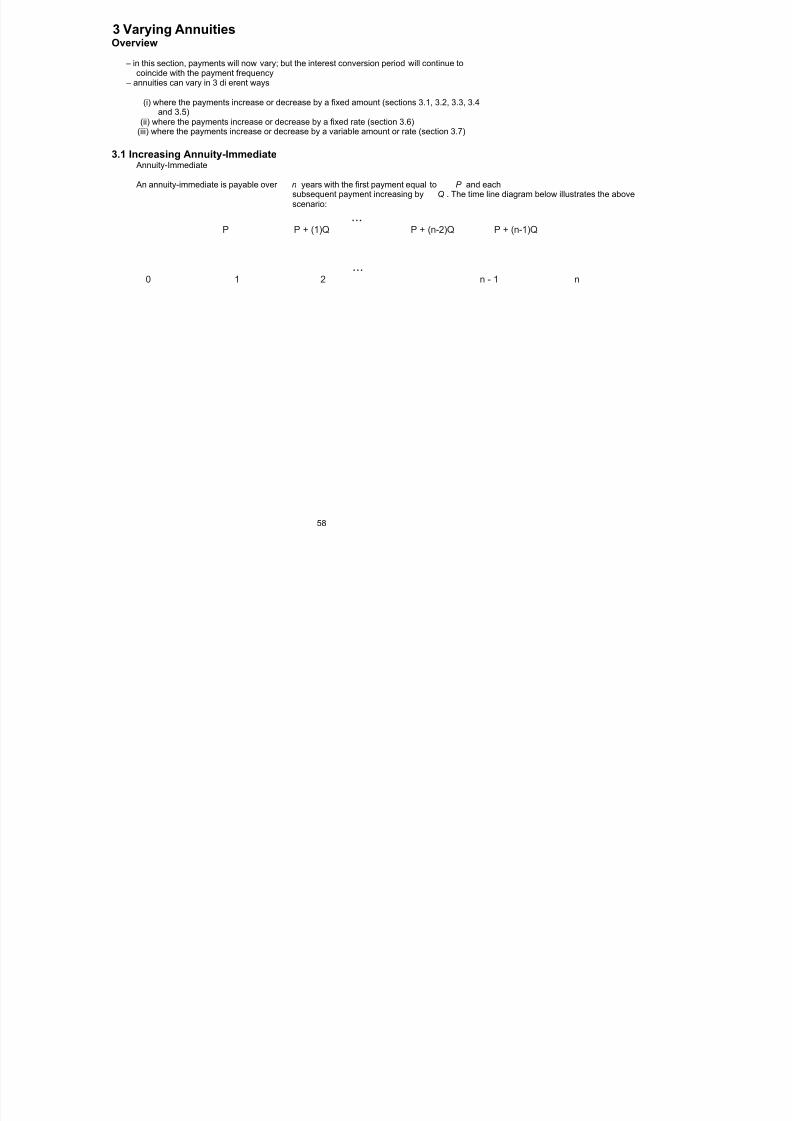
3.1 Increasing Annuity-ImmediateAnnuity-Immediate
An annuity-immediate is payable over n years with the first payment equal to P and each
subsequent payment increasing by Q . The time line diagram below illustrates the abovescenario:
...P P + (1)Q P + (n-2)Q P + (n-1)Q
...0 1 2 n - 1 n
58

8/8/2019 3500145 Financial Math for Actuary and Businessman
http://slidepdf.com/reader/full/3500145-financial-math-for-actuary-and-businessman 61/181
The present value (at t = 0) of this annual a nnuity–immediate, where the annual e ectiverate of interest is i , shall be calculated as follows:
PV =[ P ] v +[ P + Q ] v + ··· +[ P +( n - 2) Q ] v +[ P +( n - 1) Q ] v 2 n - 1 n
0
= P [ v + v + ··· + v + v ]+ Q [ v +2 v ··· +( n - 2) v +( n - 1) v ] 2 n - 1 n 2 3 n - 1 n
= P [ v + v + ··· + v + v ]+ Qv [1 + 2 v ··· +( n - 2) v +( n - 1) v ] 2 n - 1 n 2 n - 3 n - 2
d = P [ v + v + ··· + v + v ]+ Qv [1 + v + v + ··· + v + v ] 2 n - 1 n 2 2 n - 2 n - 1
dv d
= P · a + Qv [¨ a ] 2
n n dv i i
d 1 - v n= P · a + Qv 2
n dv 1 - v i
(1 - v ) · ( -nv ) - (1 - v ) · ( - 1) n - 1 n
= P · a + Qv 2n (1 - v ) 2 i
Q -nv ( v - 1) + (1 - v ) n - 1 n
= P · a +n (1 + i ) ( i/ 1+ i ) 2 2 i
(1 - v ) - nv - nv n n - 1 n
= P · a + Qn i 2 i
(1 - v ) - nv ( v - 1) n n - 1
= P · a + Qn i 2 i
(1 - v ) - nv (1 + i - 1) n n
= P · a + Qn i 2 i
(1 - v ) ( i ) n n
i - nv i = P · a + Q
n i i
- nv nn = P · a + Q a i
n i i
The accumulated value (at t = n ) of an annuity–immediate, where the annual e ective rateof interest is i , can be calculated using the same approach as above o r calculated by usingthe basic principle where an accumulated value is equal to its present value carried forwardwith interest:
FV = PV · (1 + i ) n
n 0
- nv nn = P · a + Q a (1 + i ) n
i
n i i
· (1 + i ) - nv · (1 + i ) n n n
n = P · a · (1 + i ) + Q a ni
n i i - n
n = P · s + Q si
n i i
59

8/8/2019 3500145 Financial Math for Actuary and Businessman
http://slidepdf.com/reader/full/3500145-financial-math-for-actuary-and-businessman 62/181
Let P =1and Q = 1. In this case, the payments start at 1 and increase by 1 every year until the final payment of n is made at time n .
...1 2 n - 1 n
...0 1 2 n - 1 n
Increasing Annuity-Immediate Present Value Factor The present value (at t = 0) of this annual increasing annuity–immediate, where the annuale ective rate of interest is i , shall be denoted a s ( Ia ) and is calculated as follows:
ni
- nv n
n ( Ia )=(1) · a
+(1) · ai
n n i i i
- v a - nv n n
n = 1 +i
i i - v + a - nv n n
n = 1i
i a - nv n
n = ¨i
i
Increasing Annuity-Immediate Accumulation Factor The accumulated value (at t = n ) of this annual increasing annuity–immediate, where theannual e ective rate of interest is i , shall be denoted as ( Is ) and can be calculated using
ni
the same g eneral approach as above, or alternatively, by simply using the basic principlewhere an accumulated value is equal to its present value carried forward with interest:
( Is ) =( Ia ) · (1 + i ) n
n ni i
a - nv nn = ¨ (1 + i ) n
i
i ·a · (1 + i ) - nv · (1 + i ) n n n
n = ¨ i
i s - n
n = ¨i
i
60

8/8/2019 3500145 Financial Math for Actuary and Businessman
http://slidepdf.com/reader/full/3500145-financial-math-for-actuary-and-businessman 63/181
Increasing Perpetuity-Immediate Present Value Factor The present value (at t = 0) of this annual increasing perpetuity–immediate, where theannual e ective rate of interest is i , shall be denoted as ( Ia ) and is calculated as follows:
8 i
( I a ) = v +2 v +3 v + ... 2 38
v ( Ia ) = v +2 v +3 v + ... 2 3 48
( I a ) - v ( Ia ) = v + v + v + ... 2 38 8
( Ia ) (1 - v )= a8 8
i a a i 8 8 ( Ia ) = = = = 1+ d
8 1 - v d i i 21+ i
3.2 Increasing Annuity-Due
An annuity-due is payable over n years with the first payment equal to P and each subsequentpayment increasing by Q . The time line diagram below illustrates the above scenario:
...P P + (1)Q P + (2)Q P + (n-1)Q
...0 1 2 n - 1 n
61
8/8/2019 3500145 Financial Math for Actuary and Businessman
http://slidepdf.com/reader/full/3500145-financial-math-for-actuary-and-businessman 64/181
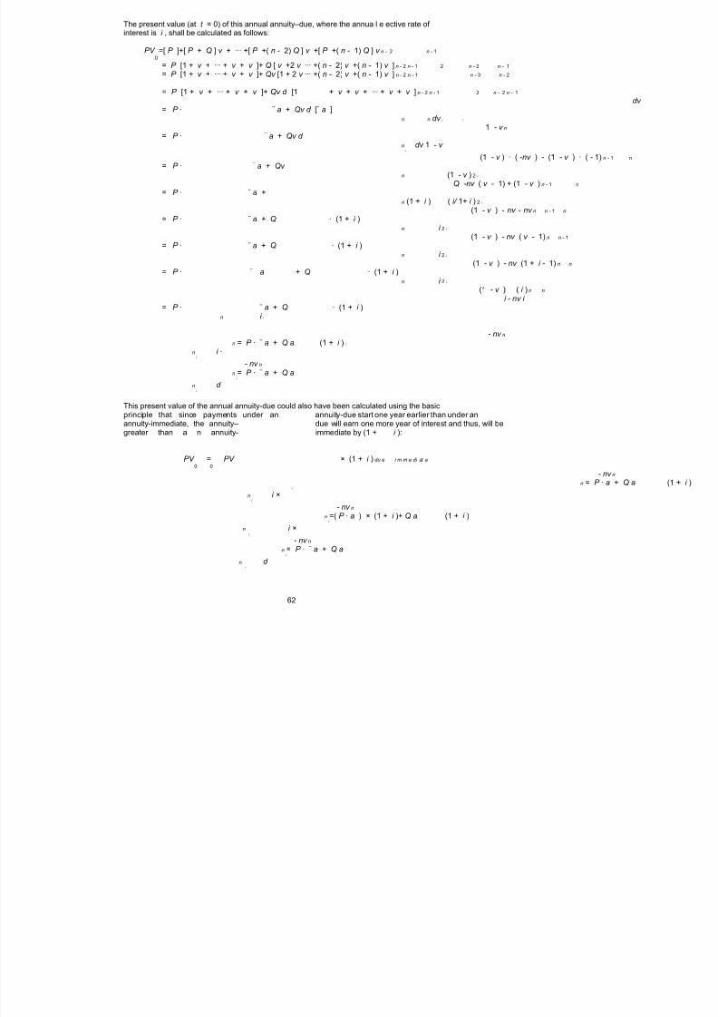
The present value (at t = 0) of this annual annuity–due, where the annua l e ective rate of interest is i , shall be calculated as follows:
PV =[ P ]+[ P + Q ] v + ··· +[ P +( n - 2) Q ] v +[ P +( n - 1) Q ] v n - 2 n - 10
= P [1 + v + ··· + v + v ]+ Q [ v +2 v ··· +( n - 2) v +( n - 1) v ] n - 2 n - 1 2 n - 2 n - 1
= P [1 + v + ··· + v + v ]+ Qv [1 + 2 v ··· +( n - 2) v +( n - 1) v ] n - 2 n - 1 n - 3 n - 2
= P [1 + v + ··· + v + v ]+ Qv d [1 + v + v + ··· + v + v ] n - 2 n - 1 2 n - 2 n - 1
dv = P · ¨ a + Qv d [¨ a ]
n n dv i i
1 - v n= P · ¨ a + Qv d
n dv 1 - v i
(1 - v ) · ( -nv ) - (1 - v ) · ( - 1) n - 1 n
= P · ¨ a + Qv
n (1 - v ) 2 i
Q -nv ( v - 1) + (1 - v ) n - 1 n
= P · ¨ a +n (1 + i ) ( i/ 1+ i ) 2 i
(1 - v ) - nv - nv n n - 1 n
= P · ¨ a + Q · (1 + i )n i 2 i
(1 - v ) - nv ( v - 1) n n - 1
= P · ¨ a + Q · (1 + i )n i 2 i
(1 - v ) - nv (1 + i - 1) n n
= P · ¨ a + Q · (1 + i )n i 2 i
(1 - v ) ( i ) n n
i - nv i = P · ¨ a + Q · (1 + i )
n i i
- nv nn = P · ¨ a + Q a (1 + i ) i
n i ·i
- nv nn = P · ¨ a + Q a
i
n d i
This present value of the annual annuity-due could also have been calculated using the basicprinciple that since payments under an annuity-due start one year earlier than under anannuity-immediate, the annuity– due will earn one more year of interest and thus, will begreater than a n annuity- immediate by (1 + i ):
PV = PV × (1 + i ) du e i m m e di at e
0 0
- nv nn = P · a + Q a (1 + i )
i
n i ×i
- nv nn =( P · a ) × (1 + i )+ Q a (1 + i )
i
n i ×i
- nv nn = P · ¨ a + Q a
i
n d i
62

8/8/2019 3500145 Financial Math for Actuary and Businessman
http://slidepdf.com/reader/full/3500145-financial-math-for-actuary-and-businessman 65/181
The accumulated value (at t = n ) of an annuity–due, where the annual e ective rate of interest is i , can be calculated using the same general approach as above, or alternatively,calculated by using the basic principle where an accumulated value is equal to its presentvalue carried fo rward with interest:
FV = PV · (1 + i ) n
n 0
- nv nn = P · ¨ a + Q a (1 + i ) n
i
n d i
· (1 + i ) - nv · (1 +i ) n n n
n = P · ¨ a · (1 + i ) + Q a ni
n d i
- nn = P · s ¨ + Q s
i
n d i
63

8/8/2019 3500145 Financial Math for Actuary and Businessman
http://slidepdf.com/reader/full/3500145-financial-math-for-actuary-and-businessman 66/181
Let P =1and Q = 1. In this case, the payments start at 1 and increase by 1 every year until the final payment of n is made at time n - 1.
...1 2 3 n
...0 1 2 n - 1 n
Increasing Annuity-Due Present Value Factor The present value (at t = 0) of this a nnual increasing annuity–due, where the annual e ectiverate of interest is i , shall be denoted as ( I ¨ a ) and is calculated as follows:
ni
-nv n
n ( I ¨a ) =(1) · ¨a +(1) · a
i
n n d i i
- v a - nv n n
n = 1 +i
d d - v + a - nv n n
n = 1i
d a - nv n
n = ¨i
d
Increasing Annuity-Due Accumulated Value Factor The accumulated value (at t = n ) of this annual increasing annuity–immediate, where theannual e ective rate of interest is i , shall be denoted as ( I s ¨ ) and can be calculated using
ni
the same approach as above or by simply using the basic principle where an accumulatedvalue is equal to its present value carried forward with interest:
( I s ¨ ) =( I ¨ a ) · (1 + i ) n
n ni i
a - nv nn = ¨ (1 + i ) n
i
d ·a · (1 + i ) - nv · (1 + i ) n n n
n = ¨i
d s - n
n = ¨i
d
64

8/8/2019 3500145 Financial Math for Actuary and Businessman
http://slidepdf.com/reader/full/3500145-financial-math-for-actuary-and-businessman 67/181
Increasing Perpetuity-Due Present Value Factor The present value (at t=0 ) of this annual increasing perpetuity-due, where the annual e ectiverate of interest is i , shall be denoted as ( I ¨ a ) and is calculated as follows:
8 i
( I ¨ a ) =1+2 v +3 v +4 v + ... 2 38
v ( I ¨ a ) = v +2 v +3 v + ... 2 38
( I ¨ a ) - v ( I ¨ a ) =1+ v + v + ... 28 8
1 a8 ( I ¨ a ) (1 - v )= ¨ = = 1d
8 1 - v d d 2
65

8/8/2019 3500145 Financial Math for Actuary and Businessman
http://slidepdf.com/reader/full/3500145-financial-math-for-actuary-and-businessman 68/181
3.3 Decreasing Annuity-Immediate
Let P = n and Q = - 1. In this case, the payments sta rt at n and decrease by 1 every year until the final payment of 1 is made at time n .
...n n - 1 2 1
...0 1 2 n - 1 n
Decreasing Annuity-Immediate Present Value Factor The present value (at t = 0) of this annual decreasing annuity–immediate, where the annuale ective rate of interest is i , shall be denoted a s ( Da ) and is calculated as follows:
ni
-
nv nn ( Da )
=( n ) · a +( - 1) · ai
n n i i i
1 - v - nv n n
n = n ·i
i - a i n - nv - a + nv n n
n =i
i n - a
n =i i
Decreasing Annuity-Immediate Accumulation Value Factor The accumulated value (at t = n ) of this annua l decreasing a nnuity–immediate, where theannual e ective rate of interest is i , shall be denoted as ( Ds ) and can be calculated by
ni
using the same general approach a s above, or alternatively, by simply using the basic principlewhere an accumulated value is equal to its present value carried forward with interest:
( Ds ) =( Da ) · (1 + i ) n
n ni i
n - an = (1 + i ) n i
i ·n · (1 + i ) - s n
n =i
i
66

8/8/2019 3500145 Financial Math for Actuary and Businessman
http://slidepdf.com/reader/full/3500145-financial-math-for-actuary-and-businessman 69/181
3.4 Decreasing Annuity-Due
Let P = n and Q = - 1. In this case, the payments sta rt at n and decrease by 1 every year until the final payment of 1 is made at time n .
...n n - 1 n - 2 1
...0 1 2 n - 1 n
Decreasing Annuity-Due Present Value Factor The present value (at t = 0) o f this annual decreasing annuity–due, where the annual e ectiverate of interest is i , shall be denoted as ( D ¨ a ) and is calculated as follows:
ni
-nv n
n ( D ¨a ) =( n ) · a ¨ +( - 1) · a
i
n n d i i
1 - v - nv n n
n = n ·i
d - a d n - nv - a + nv n n
n =i
d n - a
n =i
d
Decreasing Annuity-Due Accumulated Value Factor The accumulated value (at t = n ) of this annual decreasing annuity–due, where the annuale ective rate of interest is i , shall be denoted as ( D ¨ s ) and can be calculated using the
ni
same appro ach as above or by simply using the basic principle where an accumulated valueis equal to its present value carried fo rward with interest:
( D s ¨ ) =(¨ Da ) · (1 + i ) n
n ni i
n - an = (1 + i ) n
i
d ·n · (1 + i ) - s n
n =i
d
67

8/8/2019 3500145 Financial Math for Actuary and Businessman
http://slidepdf.com/reader/full/3500145-financial-math-for-actuary-and-businessman 70/181
Basic Relationship 1:¨ a = i · ( Ia ) + nv nn n
Consider an n –year investment where 1 is invested at the beginning of each year. The presentvalue of this multiple payment income stream at t =0is ¨ a .
n
Alternatively, consider a n –year investment where 1 is invested at the beginning of each year and produces increasing annual interest payments progressing to n · i by the end o f the lastyear with the total payments ( n × 1) refunded at t = n .
The present value of this multiple payment income stream at t =0 is i · ( Ia ) + nv . n
n
Theref ore, the present value of both investment opportunities a re equal.
a - n · v nn Also note that ( Ia ) = ¨ ¨ a = i · ( Ia ) + nv . n
n n n i
68

8/8/2019 3500145 Financial Math for Actuary and Businessman
http://slidepdf.com/reader/full/3500145-financial-math-for-actuary-and-businessman 71/181
3.5 Continuously Payable Varying Annuities – payments are made at a continuous rate although they increase at discrete times.
Continuously Payable Increasing Annuity Present Value FactorsThe present value (at t = 0) of an increasing annuity, where payments are being madecontinuously at an annual rate t , increasing at a discrete time t and where the annual e ectiverate of interest is i , shall be denoted as ( I ¯ a ) and is calculated as follows:
ni
( I ¯ a ) =¯ a +2¯ a v +3¯ a v + ... + n ¯ a v 2 n - 1n 1 1 1 1
2 n - 1 =¯ a (1 + 2 v +3 v + ... + nv )
1
=¯ a ( I a ¨ )n 1
- v ¨ a - nv nn = 1
d · d
a - nv nn = ¨
d
Continuously Payable Increasing Annuity Accumulated Value Factor The accumulated value (at t = n ) of this annual increasing annuity where the annual e ectiverate of interest is i , shall be denoted as ( I ¯ s ) and can be ca lculated using the basic principle
ni
where an accumulated value is equal to its present value carried forward with interest.
( I s ¯ ) =(1+ i ) ( I a ¯ ) n
n n
¨ a - nv n
n =(1+ i ) n
d s - n
n = ¨d
69

8/8/2019 3500145 Financial Math for Actuary and Businessman
http://slidepdf.com/reader/full/3500145-financial-math-for-actuary-and-businessman 72/181
Continuously Payable Increasing Perpetuity Present Value Factor The present value (at t = 0) of an increasing perpetuity, where payments are being madecontinuously at an annual rate of t , increasing at a discrete time t and where the annuale ective rate of interest is i , shall be denoted a s ( I ¯ a ) and is calculated as follows:
8 i
( I ¯ a ) =¯ a +2¯ a v +3¯ a v + ... 28 1 1 1
=¯ a (1 + 2 v +3 v + ... ) 21
- v 1=¯ a ( I ¨ a ) = 1
8 d · d 1 2
= 1d · d
Continuously Payable Decreasing Annuity Present Value Factor The present value (a t t = 0) of a decreasing annuity where payments are being made con-
tinuously at an annual rate t , decreasing at a discrete time t and where the annual e ectiverate of interest is i , shall be denoted as ( D ¯ a ) and is calculated as follows:
ni
( D a ¯ ) =n a ¯ +( n - 1)¯ a v +( n - 2)¯ a v + ... +¯ a v 2 n - 1n 1 1 1 1
=¯ a ( n +( n - 1) v +( n - 2) v + ... + v ) 2 n - 11
- v n =¯ a ( D a ¨ ) =
1n d · n - a d 1
n - an =
d
Continuously Payable Decreasing Annuity Accumulated Value Factor The accumulated value (at t = n ) of this annual decreasing annuity, where the e ective rateof interest is i , shall be denoted as ( D ¯ s ) and can be calculated using the basic principle
ni
where an accumulated value is equal to its present value carried forward with interest.
( D s ¯ ) =(1+ i ) ( D ¯ a ) n
n n
n - an =(1+ i ) n
d n (1 + i ) - s n
n =d
70
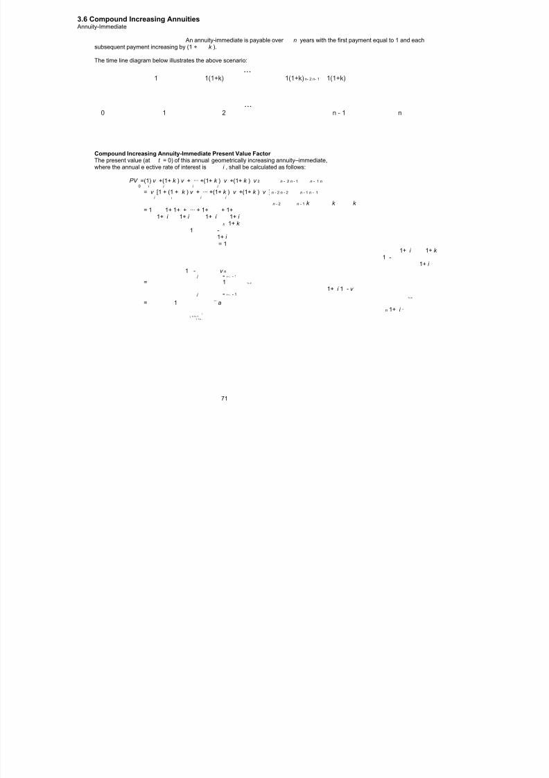
8/8/2019 3500145 Financial Math for Actuary and Businessman
http://slidepdf.com/reader/full/3500145-financial-math-for-actuary-and-businessman 73/181
3.6 Compound Increasing AnnuitiesAnnuity-Immediate
An annuity-immediate is payable over n years with the first payment equal to 1 and eachsubsequent payment increasing by (1 + k ).
The time line diagram below illustrates the above scenario:
...1 1(1+k) 1(1+k) n- 2 n- 1 1(1+k)
...0 1 2 n - 1 n
Compound Increasing Annuity-Immediate Present Value Factor The present value (at t = 0) of this annual geometrically increasing annuity–immediate,where the annual e ective rate of interest is i , shall be calculated as follows:
PV =(1) v +(1+ k ) v + ··· +(1+ k ) v +(1+ k ) v 2 n - 2 n - 1 n - 1 n
0 i i i i
= v [1 + (1 + k ) v + ··· +(1+ k ) v +(1+ k ) v ] n - 2 n - 2 n - 1 n - 1i i i i
n - 2 n - 1 k k k = 1 1+ 1+ + ··· + 1+ + 1+
1+ i 1+ i 1+ i 1+ i n 1+ k
1 -1+ i = 1
1+ i 1+ k 1 -
1+ i
1 - v n j = 1+ i - 1
= 1 1+ k
1+ i 1 - v j = 1+ i - 1
1+ k
= 1 ¨ an 1+ i ·
i j = 1+ 1
1 + k -
71

8/8/2019 3500145 Financial Math for Actuary and Businessman
http://slidepdf.com/reader/full/3500145-financial-math-for-actuary-and-businessman 74/181
Compound Increasing Annuity-Immediate Accumulated Value Factor The accumulated value (at t = n ) of an annual geometric increasing annuity-immediate,where the annual e ective rate of interest is i , can be calculated using the same approach asabove or calculated by using the basic principle where an a ccumulated value is equal to itspresent value carried forward with interest:
FV = PV · (1 + i ) n
n 0
= 1 ¨ a (1 + i ) n
n 1+ i · i
j = 1+ 11+ k -
= 1 s ¨n 1+ i · i
j = 1+ 11 + k -
72

8/8/2019 3500145 Financial Math for Actuary and Businessman
http://slidepdf.com/reader/full/3500145-financial-math-for-actuary-and-businessman 75/181
Annuity-Due
An annuity-due is payable over n years with the first payment equal to 1 and each subsequentpayment increasing by (1 + k ). The time line diagram below illustrates the above scenario:
n - 1 2 1 1(1+k) ... 1(1+k) 1(1+k)
... 0 12 n-1 n
Compound Increasing Annuity-Due Present Value Factor The present value (at t = 0) of this annual geometrica lly increasing a nnuity–due, where the
annual e ective rate of interest is i , shall be calculated as follows:n - 2 n - 2 n - 1 n - 1 PV =(1)+(1+ k ) v + ··· +(1+ k ) v +(1+ k ) v
0 i i i
n - 2 n - 1 k k k =1+ 1+ + ··· + 1+ + 1+
1+ i 1+ i 1+ i n 1+ k
1 -1+ i
=1+ k
1 -1+ i
1 - v n j = 1 + i - 1
= 1+ k
1 - v 1 + i j = - 11+ k
=¨ an
i j = 1+ 1
1 + k -
This present value could also have been achieved by simply multiplyingthe annuity-immediateversion by (1 + i ); 1 a ¨ · (1 + i ).
n 1+ i ·i
j = 1+ 11+ k -
Compound Increasing Annuity-Due Accumulated Value Factor The accumulated value (at t = n ) of an annual geometric increa sing annuity-due, where theannual e ective ra te of interest is i , can be calculated using the same approach as above or calculated by using the basic principle where an accumulated value is equal to its presentvalue carried fo rward with interest:
FV = PV · (1 + i ) n
n 0
=¨ a (1 + i ) n
ni
j = 1+ 11+ k -
=¨ sn
i j = 1+ 1
1+ k -
73

8/8/2019 3500145 Financial Math for Actuary and Businessman
http://slidepdf.com/reader/full/3500145-financial-math-for-actuary-and-businessman 76/181
3.7 Continuously Varying Payment StreamsContinuously Varying Payment Stream Present Value Factor The present value (at t=a) of this continuously varying payment stream, where the paymentstream is from t = a to t = b and the annual force of interest is d :
t t
t
d · dsb - s
· e dt a
t a
Continuously Varying Payment Stream Accumulated Value Factor The accumulated value (a t t=b) of this continuously varying payment stream, where thepayment is from t = a to t = b and the annual e ective rate of interest is d :
t
t
d · dsb
s
· e dt a
t a
74

8/8/2019 3500145 Financial Math for Actuary and Businessman
http://slidepdf.com/reader/full/3500145-financial-math-for-actuary-and-businessman 77/181
3.8 Continuously Increasing Annuities – payments are made continuously at a varying rate every year for the next n years
Continuously Increasing Annuity Present Value Factor – The present value (at t = 0) of an increasing annuity, where payments are being made
continuously at annual rate t at time t and where the annual e ective rate of interest is i ,shall be denoted as ¯ I ¯ a and is calculated as follows (using integration by parts):
ni
n
¯ I ¯ a = tv dt t n
i 0n
= t e dt -d t
0u dv n e -d t n -d t
= te --d -d dt
0 0
u ·v v ·du
n · e a -d n
n = + ¯ i
-d d a - n · v n
n = ¯ i i
d
– The present value (at t = 0) of an annuity, where payment at time t is defined as f ( t ) dt andwhere the annual e ective rate of interest is i , shall be calculated as follows:
n
f ( t ) · v dt t
i 0
– if the force of interest becomes variable then the above formula becomes:
n
f ( t ) · e dt t d dss
0
0
Continuously Increasing Annuity Accumulated Value Factor – The accumula ted value (at t = n ) of an increasing annuity, where payments are being made
continuously at annual rate t at time t and where the annual e ective rate of interest is i ,shall be denoted as ¯ I ¯ s and is calculated as follows:
ni
¯ ¯ I s ¯ =(1 + i ) I ¯ a n
n ni i
¯ a - nv nn =(1 + i ) n i
d s - n
n = ¯ i
d
75

8/8/2019 3500145 Financial Math for Actuary and Businessman
http://slidepdf.com/reader/full/3500145-financial-math-for-actuary-and-businessman 78/181
Continuously Payable Continuously Increasing Perpetuity Present Value Factor – The present value (at t = 0) of an increasing perpetuity, where payments are being made
continuously at an annual rate of t , increasing at a continuous time t and where the annuale ective rate of interest is i , shall be denoted a s ( ¯ I ¯ a ) and is calculated as follows:
8 i
8
¯ I ¯ a = tv dt t 8
i 0
a -8·v 8
8 = ¯ i i
d - 0 1
= d
d = 1
d 2
3.9 Continuously Decreasing Annuities – payments are made continuously at a varying rate every year for the next n years
Continuously Decreasing Annuity Present Value Factor – The present value (at t = 0) of a decreasing annuity where payments are being made contin-
uously at an annual rate t , decreasing at a continuous time t and where the annual e ectiverate of interest is i , shall be denoted as ( ¯ D ¯ a ) and is calculated as follows:
ni
n
( ¯ D ¯ a ) = ( n - t ) · v dt t n
i
0n n
= n v dt - t · v dt t t
0 0 ¯ a n ( ¯ I ¯ a )
n
¯ a - nv nn = n · ¯ a -
n d n · (1 - v ) - a ¯ + nv n n
n =d
n - ¯ an =
d
Continuously Decreasing Annuity Accumulated Value Factor The accumulated value (at t = n ) of this annual decreasing annuity, where the e ective rateof interest is i , shall be denoted as ( ¯ D ¯ s ) and can be calculated using the basic principle
ni
where an accumulated value is equal to its present value carried forward with interest.( ¯ D ¯ s ) =(1 + i ) ( ¯ D ¯ a ) n
n ni i n - a ¯
n =(1+ i ) n
i
d n (1 + i ) - s ¯ n
n =i
d
76

8/8/2019 3500145 Financial Math for Actuary and Businessman
http://slidepdf.com/reader/full/3500145-financial-math-for-actuary-and-businessman 79/181
Exercises and Solutions3.1 Increasing Annuity-Immediate
Exercise (a)A deposit of 1 is made at the end of each year for 10 years into a bank account that paysinterest at the end of each year at an annual e ective rate of j .Each interest payment is reinvested into another account where it earns an annual e ective
j interest rate of .2
The accumulated value of these interest payments at the end of 10 years is 4.0122. Calculate j .Solution (a)
j · ( Is ) =4 . 01229
j 2
¨ a
9 - 9j =4 j · . 0122
2
j 2
. 0122¨ a = 4 . 0061 j j =8%
2 +9=11 2 =4% 9j
2
77

8/8/2019 3500145 Financial Math for Actuary and Businessman
http://slidepdf.com/reader/full/3500145-financial-math-for-actuary-and-businessman 80/181
Exercise (b)Youaregiventwoseriesofpayments.Series A is a perpetuity with payments of 1 at the beginning of each of the first three years,
2 at the beginning o f each of the next three years, 3 at the beginning o f each of the nextthree years, and so on.Series B is a perpetuity with payments of K at the beginning of each of the first two years,2 K at the beginning of each of the next two years, 3 K at the beginning of each of the nexttwo years, and so on.The present value of these two series is equal to each other.Determine K .Solution (b)
¨ a · ( Ia ) =( K ¨ a ) · ( Ia )8 8 3 2
i =( 1+ i )3 - 1 i =( 1+ i )2 - 1
1 1¨ a · =( K ¨ a ) ·
3 2 i d i d
1+ i 1+ i ¨ a · =( K ¨ a ) ·
i i i i 3 2
1+(1+ i ) - 1 1+(1+ i ) - 1 3 2
¨ a · =( Ka ) ·[(1 + i ) - 1] [(1 + i ) - 1] 3 2 3 2 2 2
(1 + i ) - 1 (1 + i ) (1 + i ) - 1 (1 + i ) 3 3 2 2
= K d · [(1 + i ) - 1] d · [(1 + i ) - 1] 3 2 2 2
(1 + i ) K (1 + i ) - 1 = (1 + i ) - 1 3 2
i ) - 1 s (1 + i ) v s a 2 2
K = (1 + · (1 + i )= = = 2 2 2
(1 + i ) - 1 s v s a 3 33 3 3
78
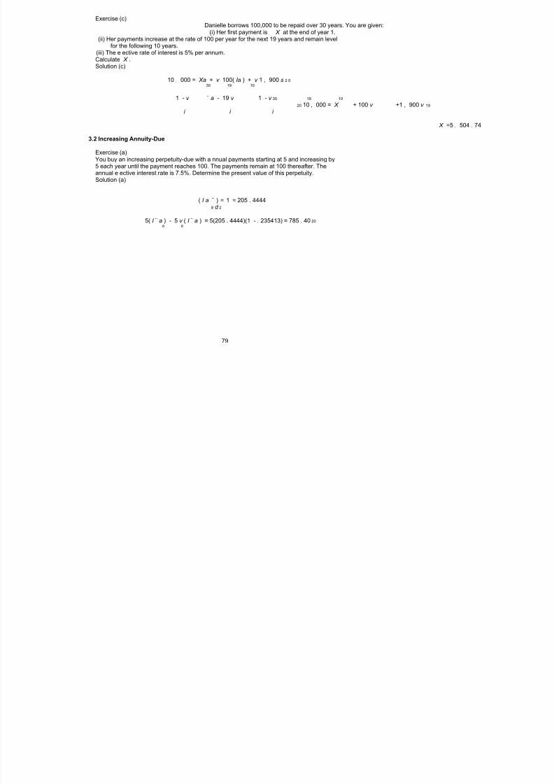
8/8/2019 3500145 Financial Math for Actuary and Businessman
http://slidepdf.com/reader/full/3500145-financial-math-for-actuary-and-businessman 81/181
Exercise (c)Danielle borrows 100,000 to be repaid over 30 years. You are given:
(i) Her first payment is X at the end of year 1.(ii) Her payments increase at the rate of 100 per year for the next 19 years and remain level
for the following 10 years.(iii) The e ective rate of interest is 5% per annum.Calculate X .Solution (c)
10 , 000 = Xa + v 100( Ia ) + v 1 , 900 a 2 030 19 10
1 - v ¨ a - 19 v 1 - v 30 19 10
20 10 , 000 = X + 100 v +1 , 900 v 19
i i i
X =5 , 504 . 74
3.2 Increasing Annuity-Due
Exercise (a)You buy an increasing perpetuity-due with a nnual payments starting at 5 and increasing by5 each year until the payment reaches 100. The payments remain at 100 thereafter. Theannual e ective interest rate is 7.5%. Determine the present value of this perpetuity.Solution (a)
( I a ¨ ) = 1 = 205 . 44448 d 2
5( I ¨ a ) - 5 v ( I ¨ a ) = 5(205 . 4444)(1 - . 235413) = 785 . 40 208 8
79

8/8/2019 3500145 Financial Math for Actuary and Businessman
http://slidepdf.com/reader/full/3500145-financial-math-for-actuary-and-businessman 82/181
3.3 Decreasing Annuity-Immediate
Exercise (a)You can purcha se one of two annuities:Annuity 1: An 11-year annuity-immediate with payments starting at 1 and then increasing
by 1 for 5 years, fo llowed by payments starting at 5 and then decreasing by 1 for 4 years.The first payment is in two years.Annuity 2: A 13-year annuity-immediate with payments starting at 5 and then increasing by2 for 5 years, followed by payments starting at 16 and then decreasing by 4 for 3 years andthen decreasing by 1 f or 3 years. The first payment is in one year.The present value of Annuity 1 is equal to 36.Determine the present va lue of Annuity 2.Solution (a)
¨ a - 6 v 5 - a 6
PV = v [pyramid annuity] = v ( Ia ) + v ( Da ) = v + v 6 6 6 5
1 i i 6 5
2 v [¨ a · a ]= a · a =[ a ] =36 a =6 i =0%6 6 6 6 6 6
PV =5+7+9+11+13+15+16+12+8+4+3+2+1=1062
Exercise (b)1,000 is deposited into Fund X , which earns an annual e ective rate of interest of i .Attheend of each year, the interest earned plus a n additional 100 is withdrawn from the fund. Atthe end of the tenth year, the fund is depleted.The annual withdrawals of interest and principal are deposited into Fund Y ,whichearnsanannual e ective rate of 9%.
The accumulated value o f Fund Y at the end of year 10 is 2,085.Determine i .
Solution (b)
10(1 . 09) - s 10 1 , 000 i 10 Ds ) + 100 · s = 100 i · (15 . 19293)
9 %
10 ( . 09 + 100 10 109 % 9 %
100 i (94 . 23) + 1 , 519 . 29 = 2 , 085 i =6%
80

8/8/2019 3500145 Financial Math for Actuary and Businessman
http://slidepdf.com/reader/full/3500145-financial-math-for-actuary-and-businessman 83/181
Exercise (c)You are given an annuity-immediate paying 10 for 10 years, then decreasing by one per year for nine years and paying one per yea r thereafter, forever. The annual e ective rate of interest
is 4%. Calculate the present value of this annuity.Solution (c)
PV =10 a + v ( Da ) + v a 10 198 10 9
- v 9 - a 1 10
=10 1 + v + v · 10 9 19
i i i
= 199 . 40
3.4 Decreasing Annuity-DueExercise (a)Debbie receives her first annual payment of 5 today. Each subsequent payment decreases by1 per year until time 4 years. After year 4, each payment increases by 1 until time 8 years.The annual interest rate is 6%. Determine the present value.
Solution (a)The present value at time 0:
5+4 v +3 v +2 v + v +2 v +3 v +4 v +5 v 2 3 4 5 6 7 8
Breaking up the payments from time 0 to time 4 is a decreasing annuity-due.
5+4 v +3 v +2 v + v =( D ¨ a ) 2 3 45
6%
( D ¨ a ) =13 . 9149035
6%
Then from time 5 to time 8 is an increasing annuity-due which is missing it’s first payment.
2 v +3 v +4 v +5 v =( I ¨ a ) 2 3 4
56%
( I a ¨ ) - 1=11 . 87573456%
PV =[( I ¨ a ) - 1] v =23 . 32 40 5 6%
6 %
81

8/8/2019 3500145 Financial Math for Actuary and Businessman
http://slidepdf.com/reader/full/3500145-financial-math-for-actuary-and-businessman 84/181
3.5 Continuously Payable Varying AnnuitiesExercise (a)
Calculate the accumulated value at time 10 years where payments are received co ntinuouslyover each year. The payment is 100 during the first year and subsequent payments increaseby 10 each year. The annual e ective rate of interest is 4%.
Solution (b)
=90¯ s + 10( I s ¯ )10 10
4 % 4%
= 90(12 . 244660) + 10(63 . 393834)
= 1165 . 41
3.6 Compounding Increasing Annuities
Exercise (a)You have just purchased an increasing annuity immediate for 75,000 that makes twentyannual payments as follows:
(i) 5 P, 10 P, ..., 50 P during years 1 through 10, and(ii) 50 P (1 . 05) , 50 P (1 . 05) , ..., 50 P (1 . 05) during years 11 through 20. 2 10
The a nnual e ective interest rate is 7% for the first 10 years and 5%, thereafter. Solve for P .Solution (a)
75 , 000 = 5 P · ( Ia ) +50 P (1 . 05) · v · v · ¨ a 105% 10 7% 10
7% j =0
¨ a - 10 v 10
10 7% 75 , 000 = 5 · P +50 P · v · (10) 107%
i 7%
, 000 , 000P = 75 = 75 . 29
427 . 8703 = 175 ¨ a - 10 v 10
10 5 + 500 · v 7 % 107%
i 7%
82

8/8/2019 3500145 Financial Math for Actuary and Businessman
http://slidepdf.com/reader/full/3500145-financial-math-for-actuary-and-businessman 85/181
Exercise (b)You have just purchased an annuity immediate for 75,000 that makes ten annual paymentsas follows:
(i) 12 . 45 P, 4 P, 6 P, 8 P, 10 P for years 1 through 5 and(ii) 10 P (1 . 07) , 10 P (1 . 07) , 10 P (1 . 07) , 10 P (1 . 07) , 10 P (1 . 07) for years 6 through 10. 2 3 4 5
The annual e ective interest rate is 5% for the first 5 years and 7%, thereafter. Solve for P .Solution (b)
75 , 000 = (10 . 45 P ) v +(2 P ) · ( Ia ) + v · v · [10 P (1 . 07)]¨ a 55 % 7% 5 5% 5
. 07 5 % i = 1 - 1=0 %1 . 07
a - 5 v 55 5 % 75 , 000 = P · 10 . 45 v
+2 ¨ + v · v · [10(1 . 07)](5) 55%
5% 7% i 5%
75 , 000 = P · (9 . 9524 + 25 . 1328 + 39 . 1763) = P · (74 . 2615) P =1 , 009 . 94 .
Exercise (c)You have just purchased an increasing annuity-immediate for 50,000 that makes twenty
annual payments as follows:(i) P, 2 P, ..., 10 P in years 1 through 10; and
(ii) 10 P (1 . 05) , 10 P (1 . 05) , ..., 10 P (1 . 05) in years 11 through 20. 2 10
The annual e ective interest rate is 7% for the first 10 years and 5% thereafter. Calculate P .Solution (c)
(1 . 05) (1 . 05) (1 . 05) 2 10
50 , 000 = P ( Ia ) + 10 P P + ... +10 P v 10
(1 . 05) +10 (1 . 05) (1 . 05) 10 7 % 2 107%
¨ a - 10 v 10
50 , 000 = P +[10 P · 10] v 10 10
7% i
, 000 , 000P = 50 = 5085 . 57406 ¨ a - 10 v 10
+ 100 v 10 10i 7%
P = 584 . 29
83

8/8/2019 3500145 Financial Math for Actuary and Businessman
http://slidepdf.com/reader/full/3500145-financial-math-for-actuary-and-businessman 86/181
3.7 Continuously Varying Payment Streams
Exercise (a)Find the present value of a continuous increasing annuity with a term of 10 years if the forceof interest is d =0 . 04 and if the rate of payment at time t is t per annum. 2
Solution (a)
n 10
t e dt = t e dt 2 -d ·t 2 - 0 . 04 t
0 0
Using integration by parts:
10 10 2
- 0 . 04 t - 0 . 04 t = - t e + 2 t · e dt 0 . 04 0 . 04
0 0
10 10 2 t 10 2
= - e - e + 2 e dt - 0 . 0 4(10) - 0 . 04 t - 0 . 04 t
0 . 04 (0 . 04) (0 . 04) 2 20 0
10 10 20 2 2
= - e - e - e - 0 . 4 - 0 . 04(1 0) - 0 . 04 t
0 . 04 (0 . 04) (0 . 04) 2 30
10 20 2 2
= - e - e - e + 2 - 0 . 4 -. 4 - 0 . 04(10)
0 . 04 (0 . 04) (0 . 04) (0 . 04) 2 3 3
10 2
= 2 - e + 2 - 0 . 4
(0 . 04) 0 . 04 + 20 (0 . 04) (0 . 04) 3 2 3
= 247 . 6978
84

8/8/2019 3500145 Financial Math for Actuary and Businessman
http://slidepdf.com/reader/full/3500145-financial-math-for-actuary-and-businessman 87/181
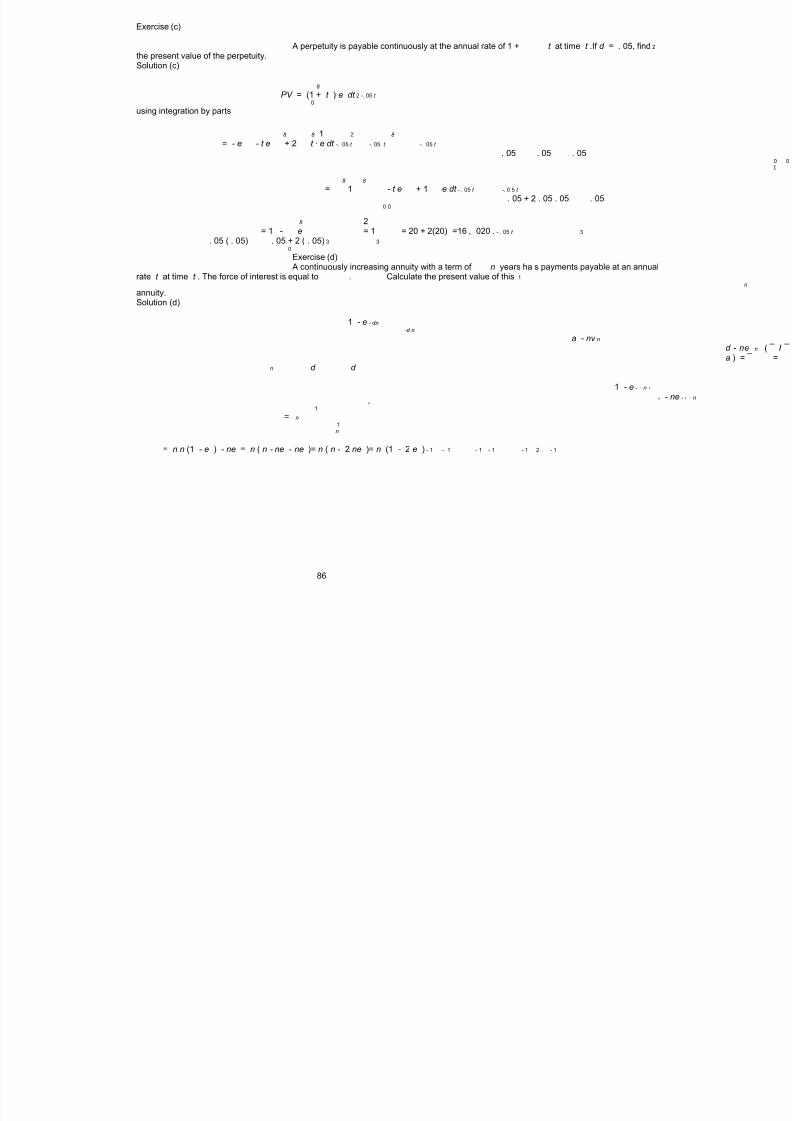
8/8/2019 3500145 Financial Math for Actuary and Businessman
http://slidepdf.com/reader/full/3500145-financial-math-for-actuary-and-businessman 88/181
Exercise (c)
A perpetuity is payable continuously at the annual rate of 1 + t at time t .If d = . 05, find 2
the present value of the perpetuity.Solution (c)
8
PV = (1 + t ) e dt 2 -. 05 t
0
using integration by parts
8 8 1 2 8
= - e - t e + 2 t · e dt -. 05 t -. 05 t -. 05 t
. 05 . 05 . 050 00
8 8
= 1 - t e + 1 e dt - . 05 t -. 0 5 t
. 05 + 2 . 05 . 05 . 050 0
8 2= 1 - e = 1 = 20 + 2(20) =16 , 020 . - . 05 t 3
. 05 ( . 05) . 05 + 2 ( . 05) 3 30
Exercise (d)A continuously increasing annuity with a term of n years ha s payments payable at an annual
rate t at time t . The force of interest is equal to . Calculate the present value of this 1n
annuity.Solution (d)
1 - e - dn
-d n
a - nv nd - ne n ( ¯ I ¯ a ) = ¯ =
n d d
1 - e- · n 1
n - ne - 1 · nn
1
= n
1n
= n n (1 - e ) - ne = n ( n - ne - ne )= n ( n - 2 ne )= n (1 - 2 e ) - 1 - 1 - 1 - 1 - 1 2 - 1
86

8/8/2019 3500145 Financial Math for Actuary and Businessman
http://slidepdf.com/reader/full/3500145-financial-math-for-actuary-and-businessman 89/181
3.9 Continuously Decreasing AnnuitiesExercise (a)
Find the ratio of the total payments made under ( ¯ D ¯ a ) during the second half of the term10
of the annuity to those made during the first half.Solution (a)
The payment is (10 - t ) · dt at time t.During the second half the total payment is:
1 0 (10 - t ) 10 2
(10 - t ) dt = - =12 . 52
5 5
During the first half the total payment is:
5 5 (10 - t ) 2
(10 - t ) dt = - =37 . 520 0
The ratio is:
. 5= 12
37 . 5 = 1 3
87

8/8/2019 3500145 Financial Math for Actuary and Businessman
http://slidepdf.com/reader/full/3500145-financial-math-for-actuary-and-businessman 90/181
4 Non-Annual Interest Rate and AnnuitiesOverview
– an e ective ra te of interest, i , is paid once per year at the end of the year – a nominal rate of interest, i , is paid more frequently during the year ( p times) and a t the ( p )
end of the sub-period (nominal rates are also quoted as annual rates) – nominal rates are adjusted to re ect the rate to be paid during the sub–period; for example,
i is the nominal rate of interest convertible semi-annually (2 )
(2 )
i = 10% i (2 )
2 = 10% 2 = 5% paid every 6 months
4.1 Non-Annual Interest and Discount RatesNon-Annual pthly E ective Interest Rates
– with e ective interest, you have interest i ,paidat p periods per year
(1 + i ) - 1 1
p
Non-Annual pthly E ective Discount Rates
– with e ective discount, you have discount d ,paidat p periods per year
1 - (1 - d ) =1 - (1 + i ) 1 - 1
p p
4.2 Nominal p Interest Rates: i thly ( p )
Equivalency to E ective Rates of Interest: i, i ( p )
– with e ective interest, you have interest, i , paid at the end of the year i ( p )
– with nominal interest, you have interest , paid at the end of each sub-perio d and this is p
done p times over the year ( p sub-perio ds per year)
p i ( p )
(1 + i )= 1+ p
– if given an e ective rate of interest, a nominal rate of interest can be determined:
1 /p i = p [(1 + i ) - 1] ( p )
– if given an e ective rate of interest, the interest rate per sub-perio d can be determined:i ( p )
1 /p =(1+ i ) - 1 p
88

8/8/2019 3500145 Financial Math for Actuary and Businessman
http://slidepdf.com/reader/full/3500145-financial-math-for-actuary-and-businessman 91/181
4.3 Nominal p Discount Rates: d thly ( p )
Equivalency to E ective Rates of Discount: d, d ( p )
– with e ective discount, you have discount, d , paid at the beginning of the year d ( p )
– with nominal discount, you have discount , pa id at the beginning of each sub-period and p
this is done p times over the year ( p sub-periods per year)
p( p )
(1 - d )= 1 - d p
– if given an e ective rate of discount, a nominal rate of discount can be determined
1 /p d = p [1 - (1 - d ) ] ( p )
– the discount rate per sub-period can be determined, if given the e ective discount rate
d ( p )
1 /p =1 - (1 - d ) p
i d ( p ) ( p )
Relationship Between and p p
– when using e ective rates, you must have (1 + i )or(1 - d ) by the end of the year - 1
- 1 (1 + i )= 1 = 1 - d )v (1 - d ) =(1
– when replacing the e ective rate formulas with their nominal rate counterparts, you have
m - p
i ( m ) ( p )
1+ = 1 - d
m p
89

8/8/2019 3500145 Financial Math for Actuary and Businessman
http://slidepdf.com/reader/full/3500145-financial-math-for-actuary-and-businessman 92/181
–when p = m
m -m i ( m ) ( m )
1+ = 1 - d m m
- 1 i ( m ) ( m )
1+ = 1 - d m mi m ( m )
1+ =m m · d ( m )
i m m - m + d ( m ) ( m )
= - 1=m m · d m - d ( m ) ( m )
i d ( m ) ( m )
=m m - d ( m )
d ( m )
i ( m ) m=
m ( m )
1 - d m
– the interest rate over the sub-period is the ratio of the discount paid to the amount at thebeginning of the sub-period (principle of the interest rate still holds)
i ( m )
d ( m ) m=
m i ( m )
1+m
– the discount rate over the sub–period is the ratio of interest paid to the amount at the endof the sub-period (principle of the discount rate still holds)
– the di erence between interest paid at the end and at the beginning of the sub-period dependson the di erence that is borrowed at the beginning of the sub-period and on the interestearned o n that di erence (principle of the interest and discount rates still holds)
i i ( m ) ( m ) ( m ) ( m ) = 1 - 1 - d m - d m m m
i ( m ) ( m )
= 0m · d m =
90

8/8/2019 3500145 Financial Math for Actuary and Businessman
http://slidepdf.com/reader/full/3500145-financial-math-for-actuary-and-businessman 93/181
4.4 Annuities-Immediate Payable p thly
Present Value Factor for a p Annuity-Immediate th ly
1 1 –paymentsof are made at the end of every th of year for the next n years p p
– the present value (at t =0)ofan p ly annuity–immediate, where the annual e ective rate th
( p ) of interest is i , shall be denoted as a andis calculated as follows:
ni
p - 1 p 1 2 ( p ) a =(1 ) v +(1 ) v + ··· +(1 ) v +(1 ) v (1 st year)
p p p p
p p p pn i i i i i
p +1 2 p- 1 2 p p +2
+(1 ) v +(1 ) v + ··· +(1 ) v +(1 ) v (2 nd year) p p p m
p p p pi i i i
...
( n - 1) p +1 ( n - 1) p +2 np - 1 np
+(1 ) v +(1 ) v + ··· +(1 ) v +(1 ) v (last year) p p p p
p p p pi i i i
p - 2 p- 1 1 1
=(1 ) v 1+ v + ··· + v + v (1 st year) p p p p
p i i i i
p +1 1 p- 2 p- 1
+(1 ) v 1+ v + ··· + v + v (2 nd year) p p p p
p i i i i
.
.
.
( n - 1) p +1 p - 2 p - 1 1
+(1 ) v 1+ v + ··· + v + v (last year) p p p p
p i i i i
p +1 p - 2 p- 1 1 ( n- 1 ) p +1 ) 1
= ( 1 ) v +(1 ) v + ··· +(1 ) v 1+ v + ··· + v + v p p p p p m
p p pi i i i i i
1
- ( v ) p p p 1 1 ( n - 1) =(1 ) v 1+ v + ··· + v i p p
p i i i 1
1 - v pi
1 - v - v n 1
1 =(1 ) 1 · i i
p 1 - v 1 (1 + i ) 1 1
1 - v i p p
i - v n
1 i =(1 ) 1 p (1 + i ) 1 1
1 - v p p
i
- v ni =(1 ) 1
p (1 + i ) - 1 1
p
- v n= 1 i
p (1 + i ) - 1 1
p
- v 1 - v n n
i i = 1 = 1i p × p · i ( p ) ( p )
91

8/8/2019 3500145 Financial Math for Actuary and Businessman
http://slidepdf.com/reader/full/3500145-financial-math-for-actuary-and-businessman 94/181
Accumulated Value Factor for a p Annuity-Immediate thl y
– the accumulated value (at t = n )ofan p ly annuity–immediate, where the annual e ective th
( p ) rate of interest is i , shall bedenoted as s and is calculated as
follows:n
i
( p ) s =(1 ) + (1 )(1 + i ) + ··· +(1 )(1 + i ) +(1 )(1 + i ) (last year) 1 p - 2 p -
1 p p p
p p p pni
+(1 )(1 + i ) +(1 )(1 + i ) + ··· +(1 )(1 + i ) +(1 )(1 + i ) (2 nd last year) p p +1 2 p - 2 2 p - 1
p p p p
p p p p.
.
.
( n - 1) p ( n- 1) p +1 np- 2 np - 1 +(1 )(1 + i ) +(1 )(1 + i ) + ··· +(1 )(1 + i ) +(1 )(1 + i ) (first year) p m m pp p p p
=(1 ) 1+(1+ i ) + ··· +(1+ i ) +(1+ i ) (last year) 1 p - 2 p - 1
p p pp+(1 )(1 + i ) 1+(1+ i ) + ··· +(1+ i ) +(1+ i ) (2 nd last year) p 1 p - 2 p- 1
p p p p
p...
( n - 1) p p- 2 p - 1 +(1 )(1 + i ) 1+(1+ i ) + ··· +(1+ i ) +(1+ i ) (first year) 1
p p p p
p
p ( n- 1 ) p p -2 p - 1 = ( 1 )+(1 )(1 + i ) + ··· +(1 )(1 + i ) 1+(1+ i ) + ··· +(1+ i ) +(1+ i ) ) 1
p p p p p
p p p1 - ((1 + i ) ) 1 p
p p =(1 ) 1+(1+ i ) + ··· +(1+ i ) ( n - 1) p
p 1 - (1 + i ) 1
p
- (1 + i ) 1 - (1 + i ) n 1
=(1 ) 1 · p 1 - (1 + i ) 1 1 - (1 + i ) 1
p
- (1 + i ) n
=(1 ) 1 p 1 - (1 + i ) 1
p
i ) - 1 n
= (1 + p (1 + i ) - 1 1
p
i ) - 1 (1 + i ) - 1 n n
= (1 + = 1 p × p · i i ( p ) ( p )
92

8/8/2019 3500145 Financial Math for Actuary and Businessman
http://slidepdf.com/reader/full/3500145-financial-math-for-actuary-and-businessman 95/181
( p ) Basic Relationship 1:1= i · a + v ( p ) n
n
Basic Relationship 2: PV (1 + i ) = FV and PV = FV · v n n
( p ) – if the future value at time n , s , is discounted back totime 0, then you will have its presentn
( p ) value, an
i ) - 1 n
( p ) s · v = (1 + · v n n
i n ( p )
i ) · v - v n n n
= (1 +i ( p )
- v n= 1
i ( p )
( p ) = an
( p ) – if the present value at time 0, a , is accumulatedforward to time n , then you will have itsn
( p ) future value, sn
- v n( p ) n n a · (1 + i ) = 1 (1 + i )n i ( p )
i ) - v (1 + i ) n n n
= (1 +i ( p )
i ) - 1 n
= (1 +i ( p )
( p ) = sn
i i ( p ) ( p ) Basic Relationship 3: a = · a , s = · s
n n n n
i i ( p ) ( p )
–Considerpaymentsof made at the end of every th of year for the next n years. Over a 1 1 p p
one-year period, payments of made at the end of each p period will accumulate at the 1 th
p
( p ) end of the year to a lump sum of × p · s . If this end-of-year lump sum exists for each 1
p 1
year of the n -year annuity-immediate, then the present value (at t = 0) of these end-of-year ( p ) lump sums is the same as × p · a : 1
p n
1( p ) ( p ) = 1 · a
n p × p · a p × p · s n 1
i ( p ) a = · a
n i n ( p )
– Therefore, the accumulated value (at t = n ) of these end-o f-year lump sums is the same as( p ) × p · s : 1n p
1( p ) ( p ) = 1 · s
n n p × p · s m × p · s 1
i ( p ) s = · s
n i n ( p )
93

8/8/2019 3500145 Financial Math for Actuary and Businessman
http://slidepdf.com/reader/full/3500145-financial-math-for-actuary-and-businessman 96/181
4.5 Annuities-Due Payable p thly
Present Value Factor of a p Annuity-Due th ly
1 1 –paymentsof are made at the beginning of every th of year for the next nyears
p p
– the present value (at t =0)ofan p ly annuity–due, where the annual e ective rate of interest th
( p ) is i , shall be denoted as ¨ a and is calculated as follows:n
i
p- 2 p- 1 1 ( p ) ¨ a =( 1 )+(1 ) v + ··· +(1 ) v +(1 )v (1 st year)
p p p
p p p pn i i i i
p p +1 2 p - 2 2 p- 1
+( 1 ) v +(1 ) v + ··· +(1 ) v +(1 ) v (2 nd year) p p p p
p p p pi i i i
...
( n - 1) p ( n- 1 ) p +1 n p- 2 np- 1
+ ( 1 ) v +(1 ) v + ··· +(1 ) v +(1 ) v (last year) p p p p
p p p pi i i i
p - 2 p - 1 1
=( 1 ) 1+ v + ··· + v + v (1 st year) p p p
p i i i
p 1 p - 2 p - 1
+( 1 ) v 1+ v + ··· + v + v (2 nd year) p p p p
p i i i i
.
.
.
( n - 1) p p- 2 p- 1 1
+( 1 ) v 1+ v + ··· + v + v (last year) p p p p
p i i i i
p ( n - 1) p ) p- 2 p - 1 1
= ( 1 )+(1 ) v + ··· +(1 ) v 1+ v + ··· + v + v p p p p p
p p pi i i i i
1
- ( v ) p p p 1 ( n - 1) =( 1 ) 1+ v + ··· + v i p
p i i 1
1 - v pi
- v - v n 1
1 =( 1 ) 1 · i i
p 1 - v 1 1
1 - v i p
i - v n
1 i =( 1 ) p 1
1 - v p
i
- v ni =( 1 ) 1
p 1 - (1 - d ) 1
p
- v n= 1 i
p 1 - (1 - d ) 1
p
- v 1 - v n n
i i =1 = 1d p × p · d ( p ) ( p )
94

8/8/2019 3500145 Financial Math for Actuary and Businessman
http://slidepdf.com/reader/full/3500145-financial-math-for-actuary-and-businessman 97/181
– the accumulated value (at t = n )ofan p ly annuity–due, where the annual e ective rate of th( p ) interest is i , shall be denoted as ¨ s and iscalculated as follows:n
i
( p ) s ¨ =(1 )(1 + i ) +(1 )(1 + i ) + ··· +(1 )(1 + i ) +(1 )(1 + i ) (la st year) 1 2
p - 1 p p p p p
p p p pni
+(1 )(1 + i ) +(1 )(1 + i ) + ··· +(1 )(1 + i ) +(1 )(1 + i ) (2 nd last year) p +1 p +2 2 p - 1 2 p
p p p p
p p p p..
.
( n - 1) p +1 ( n- 1 ) p +2 np - 1 np +(1 )(1 + i ) +(1 )(1 + i ) + ··· +(1 )(1 + i ) +(1 )(1 +i ) (first year)
p p p pp p p p
p - 2 p- 1 =(1 )(1 + i ) 1+(1+ i ) + ··· +(1+ i ) +(1+ i ) (last year) 1 1
p p p pp+(1 )(1 + i ) 1+(1+ i ) + ··· +(1+ i ) +(1+ i ) (2 nd last year) p +1 1 p- 2 p- 1
p p p pp...
( n - 1) p +1 p - 2 p - 1 +(1 )(1 + i ) 1+(1+ i ) + ··· +(1+ i ) +(1+ i ) (first year) 1
p p p p
p
1 - ((1 + i ) ) 1 p
p ( n- 1) p +1 = ( 1 )(1 + i ) +(1 )(1 + i ) + ··· +(1 )(1 + i ) 1 p + 1 ) p p p
p p p 1 - (1 + i ) 1
p
1 - ((1 + i ) ) 1 p
p p =(1 )(1 + i ) 1+(1+ i ) + ··· +(1+ i ) 1 ( n - 1) p p
p 1 - (1 + i ) 1 p
1 - (1 + i ) 1 - (1 + i ) n 1
=(1 )(1 + i ) · 1
p
p 1 - (1 + i ) 1 1 - (1 + i ) 1
p
1 - (1 + i ) n
=(1 )(1 + i ) 1
p p 1 - (1 + i ) 1
p
i ) - 1 n
= (1 +1
p · v (1 + i ) - 1 1
p p
i
i ) - 1 n
= (1 +1
p 1 - v p
i
i ) - 1 n
= (1 + p 1 - (1 - d ) 1
p
i ) - 1 (1 + i ) - 1 n n
= (1 + = 1d p × p · d ( p ) ( p )
95

8/8/2019 3500145 Financial Math for Actuary and Businessman
http://slidepdf.com/reader/full/3500145-financial-math-for-actuary-and-businessman 98/181
( p ) Basic Relationship 1:1= d · ¨ a + v ( p )nn
Basic Relationship 2: PV (1 + i ) = FV and PV = FV · v n n
( p ) – if the future value at time n ,¨ s , isdiscounted back to time 0, then you will have its
n
( p ) present value, ¨ an
i ) - 1 n
( p ) s ¨ · v = (1 + · v n n
d n ( p )
i ) · v - v n n n
= (1 +d ( p )
- v n= 1
d ( p )
( p ) =¨ an
( p ) – if the present value at time 0, ¨ a , isaccumulated forward to time n , then you will haven
( p ) its future value, ¨ sn
- v n( p ) ¨ a · (1 + i ) = 1 (1 + i ) n n
d n ( p )
i ) - v (1 + i ) n n
n
= (1 +d ( p )
i ) - 1 n
= (1 +d ( p )
( p ) =¨ sn
d d
( p ) ( p ) Basic Relationship 3:¨ a = · ¨ a , s ¨ = · ¨ sn n d d n n ( p ) ( p )
–Considerpaymentsof made at the beginning of every th of year for the nextn years. 1 1 p p
Over a one-year period, payments of ma de at the beginning of each p period will 1 th
p
( p ) accumulate at the end of the year to a lump sum of × p · s ¨ . If this end-of-year 1
p 1
lump sum exists for each year of the n -year annuity-immediate, then the present value( p ) (at t = 0) o f these end-of-year lump sums is the same as × p · ¨ a : 1
p n
1( p ) ( p ) ¨ a = 1 s ¨ · a
n p × p · p × p · n 1
i ( p ) ¨ a = · a
n d n ( p )
– Therefo re, the accumulated value (at t = n ) of these end-of-year lump sums is the same( p ) as × p · s ¨ : 1
p n
1( p ) ( p ) s ¨ = 1 s ¨ · s
n p × p · p × p · n 1
i ( p ) s ¨ = · s
n n i ( p )
96

8/8/2019 3500145 Financial Math for Actuary and Businessman
http://slidepdf.com/reader/full/3500145-financial-math-for-actuary-and-businessman 99/181
Basic Relationship 5 :Due = Immediate × (1 + i ) 1
p
- v - v i n n ( p )
( p ) ( p ) ( p ) ¨ a = 1 = 1 = a · 1+ = a · (1 + i )1
p
d p n n n ( p )i ( p )
( p ) 1+ i
p i ) - 1 i ) - 1 i n n ( p )
( p ) ( p ) ( p ) s ¨ = (1 + = (1 + = s · 1+ = s · (1 + i ) 1
p
d p n n n ( p )i ( p )
( p )
1+ i
p
An p ly annuity–due starts one p of a year earlier than an p ly annuity-immediate th th th
and as a result, earns one p of a year more interest, hence it will be larger. th
97

8/8/2019 3500145 Financial Math for Actuary and Businessman
http://slidepdf.com/reader/full/3500145-financial-math-for-actuary-and-businessman 100/181
Exercises and Solutions4.2 Nominal p ly Interest Rates th
Exercise (a)100 is deposited into a bank account. The account is credited at a nominal rate of interestconvertible semiannually.
At the same time, 100 is deposited into another account where interest is credited at a forceof interest, d .After 8.25 years, the value of each account is 300.Calculate ( i - d ).Solution (a)
2 · (8 . 25) 2
i i i (2 ) ( 2 ) (2 )
100 1+ = 300 1+ =1 . 06885 i = 1+ - 1= . 142439 1
16 . 5 2 2 =3 2
OR
100(1 + i ) = 300 1+ i =3 i =3 - 1= . 142439 8 . 25 1 1
8 . 2 5 8 . 25
ln [3]100 e = 300 e =3 8 . 25 d = ln [3] d = . 133165 8 . 25 d 8 . 25 d
8 . 25 =
i - d = . 142439 - . 133165 = . 009274 = . 93%
98
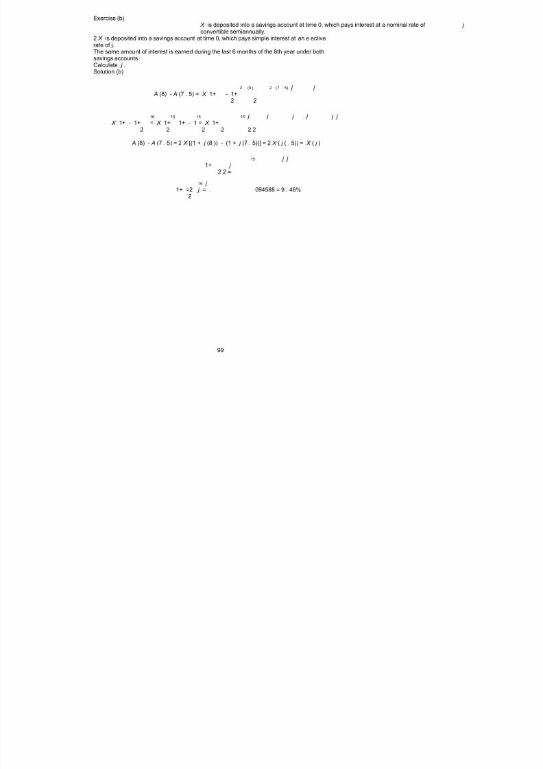
8/8/2019 3500145 Financial Math for Actuary and Businessman
http://slidepdf.com/reader/full/3500145-financial-math-for-actuary-and-businessman 101/181
Exercise (b) X is deposited into a savings account at time 0, which pays interest at a nominal rate of j convertible semiannually.
2 X is deposited into a savings account at time 0, which pays simple interest at an e ectiverate of j.The same amount of interest is earned during the last 6 months of the 8th year under bothsavings accounts.Calculate j .Solution (b)
2 · (8 ) 2 · (7 . 5) j j A (8) - A (7 . 5) = X 1+ - 1+
2 2
16 15 15 15 j j j j j j X 1+ - 1+ = X 1+ 1+ - 1 = X 1+
2 2 2 2 2 2
A (8) - A (7 . 5) = 2 X [(1 + j (8 )) - (1 + j (7 . 5))] = 2 X ( j ( . 5)) = X ( j )
15 j j 1+ j
2 2 =
15 j 1+ =2 j = . 094588 = 9 . 46%
2
99

8/8/2019 3500145 Financial Math for Actuary and Businessman
http://slidepdf.com/reader/full/3500145-financial-math-for-actuary-and-businessman 102/181
Exercise (c)At time 0, K is deposited into Fund X , which accumulates at a fo rce of interest of d =
t
t +3m ,2 K is deposited into Fund Y , which accumulates at a n annual
t +6 t +9.Attime 2
nominal rate of 10.25%, convertible quarterly.At time n ,where n>m , the accumulated value of each fund is 3 K .Calculate m .Solution (c)
n n
d · dt d · dt 4( n -m ) 4( n -m ) . 1025 . 1025 t t
K · e =2 K 1+ =3 K e =2 1+ =30 0
4 4
t +3 2 t +6 f ( t ) n n n
dt dt 1 ( n ) 1 1
t +6 t +9 t +6 t +9 =3 f ( t ) 2 2 2 2 e =3 e e =3 f =3 2
0 0 0
f (0)
1 n +6 n +9 22
=3 n +6 n +9=81 ( n - 6)( n + 12) = 0 n =6 2
9
4(6 -m ) . 1025 ln 3
2 1+ =3 4(6 - m )= 6 - m =4 m =2 2
4 ln 1+ . 10 254
Exercise (d)You make a deposit into a savings account, which pays interest at an annual nominal rate of i . (2 )
At the same time, your professor deposits 1,000 into a di erent savings account, which payssimple interest.
At the end of five yea rs, the forces of interest, d , on the two accounts are equal, and your 5
professor’s account has accumulated to 2,000. Calculate i . (2 )
Solution (d)
1 , 000(1 + 5 i )=2 , 000 i = 20%
i . 2d = =t 5 1+ it d 1+( . 2)(5) = 10%
2 1+ i i ( 2 ) (2 )
= e 1+ e = e d (1 ) d . 052
2 2 =
(2 ) . 05 i =2( e - 1) = 10 . 2542%
100

8/8/2019 3500145 Financial Math for Actuary and Businessman
http://slidepdf.com/reader/full/3500145-financial-math-for-actuary-and-businessman 103/181
Exercise (e)If an investment will be tripled in 8 years at a force of interest d , in how many years will aninvestment be doubled at a nominal rate of interest numerically equal to d and convertible
once every three years?Solution (e)
ln [3]e =3 d = 8 d
8
(1 + 3 d ) =2 n
3
n ln [3]3
1+ 3 =28
n ln [2]n n =6
3 = 3 =2 ln 1+ 3 l n [3 ]8
Exercise (f)Calculate the nominal rate of interest convertible once every four years that is equivalent toa nominal rate of discount convertible quarterly.Solution (f)
i = 1 i ) - 1 = 1 - d ) - 1 1 4 - 44
4 (1 + 4 (1
- 4 · 4 - 16 (4 ) (4 )
= 1 - d - 1 = 1 - d - 14 1 4 4 1 4
101
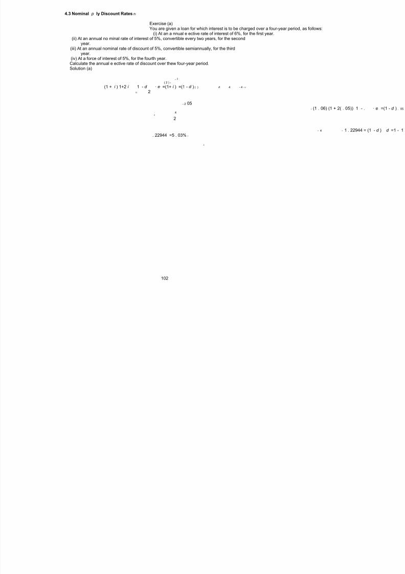
8/8/2019 3500145 Financial Math for Actuary and Businessman
http://slidepdf.com/reader/full/3500145-financial-math-for-actuary-and-businessman 104/181

8/8/2019 3500145 Financial Math for Actuary and Businessman
http://slidepdf.com/reader/full/3500145-financial-math-for-actuary-and-businessman 105/181
Exercise (b)
Express d as a function if i . (4 ) (3 )
Solution (b)
3 - 4 i (3 ) (4 )
1+ = 1 - d 3 4
- 3
i (3 )4
1 d =4 - 1+ (4 )
3
Exercise (c)
Express i as a function of d . (6 ) (2 )
Solution (c)
6 - 2
i (6 ) (2 )
1+ = 1 - d 6 2
- 1
(2 ) 3
1 i =6 - d - 1 (6 )
2
Exercise (d)Given a nominal interest rate of 7.5% convertible semiannually, determine the sum of the:
(i) force of interest; and(ii) nominal discount rate compounded monthly.
Solution (d)
2 i (2 )
1+ = e d · (1 )
2
. 075d =2 ln 1+ . 073627946
2 =
- 12 2 i (12) (12 )
1 - d = 1+12 2
- 2
i (2 ) 12
1 = d =12 - 1+ . 073402529 (12)
2
. 073627946 + . 073402529 = . 147030475
103

8/8/2019 3500145 Financial Math for Actuary and Businessman
http://slidepdf.com/reader/full/3500145-financial-math-for-actuary-and-businessman 106/181
4.4 Annuities-Immediate Payable p ly th
Exercise (a)On January 1, 1985, Michael has the following two options for repaying a loan:
(i) Sixty monthly payments of 100 beginning February 1, 1985.(ii) A single payment of 6,000 at the end of K months.
Interest is at a nominal annual rate of 12% compounded monthly. The two options have thesame present value. Determine K .Solution (a)
i (12)
. 01/month12 =
100 a = 6000 v K
60. 0 1
4495 . 5 = 6000 v K
6000. 01) K
4495 . 50 =(1
ln 6000
K = 4495 . 50
ln (1 . 01) =29 months
Exercise (b)Steve elects to receive his retirement benefit over 20 years at the rate of 2,000 per monthbeginning one month from now. The monthly benefit increases by 5% each year. At a
nominal interest rate of 6% convertible monthly, calculate the present value of the retirementbenefit.Solution (b)
R =2 , 000 s =24 , 671 . 1212
. 06. 12
PV = Rv + R (1 . 05) v + ... + R (1 . 05) v 2 19 20
20
1 - 1 . 05 1+ i
PV =24 , 671 . 12 , where i =(1 . 005) - 1= . 0616778 12 i - . 05
PV = 419 , 253 . 14
104

8/8/2019 3500145 Financial Math for Actuary and Businessman
http://slidepdf.com/reader/full/3500145-financial-math-for-actuary-and-businessman 107/181
Exercise (c)A pensioner elects to receive her retirement benefit over 20 years at a rate of 2,000 per monthbeginning one month from now. The monthly benefit increases by 5% each year.
At a nominal interest rate of 6% convertible monthly, calculate the present value of theretirement benefit.Solution (c)
2 , 000 a =23 , 237 . 8612
12 %
PV =23 , 237 . 86(1+ v (1 . 05) + v (1 . 05) + ... + v (1 . 05) ) 2 2 19 19
2 19 . 05 . 05 . 05=23 , 237 . 86 1+ 1 + 1 + ... + 1
1+ i 1+ i 1+ i
12 . 06where i = 1+ - 1= . 061678
12
20 - 1 . 05
=23 , 237 . 86 1 . 061678) 1 . 061678
. 061678 - . 05 (1
PV = 419 , 252 . 46
105

8/8/2019 3500145 Financial Math for Actuary and Businessman
http://slidepdf.com/reader/full/3500145-financial-math-for-actuary-and-businessman 108/181
Exercise (d)
(2 ) (2 ) (2 ) If 3 a =2 a =45 s , find i .n 2 n 1
Solution (d)
- v - v i n 2 n
3 1 =2 1 =45i i i (2 ) (2 ) (2 )
n 2 n 3 - 3 v =2 - 2 v
2 v - 3 v +1=0 2 n n
- 9 - 4(2)v = 3 n
4 = 1 2Then the equation:
- v i n3 1 =45
i i (2 ) (2 )
gives us
13 1 - i
2 =45
. 5i = 1
45 = 1 304.5 Annuities-Due Payable p ly th
Exercise (a)At time t =0youdeposit P into a fund which credits interest at an e ective annual interestrate of 8%. At the end of each year in years 6 through 20, you withdraw an amount su cientto purchase an annuity due of 100 per month for 10 years at a nominal interest rate of 12%
compounded monthly. Immediately after the withdrawl at the end of year 20, the fund value
is zero.Calculate P .Solution (a)
PMT = 100¨ a =7 , 039 . 75120
1 %
P (1 . 08) =7 , 039 . 75¨ a 61 5
8%
P =41 , 009 . 64
106

8/8/2019 3500145 Financial Math for Actuary and Businessman
http://slidepdf.com/reader/full/3500145-financial-math-for-actuary-and-businessman 109/181
Exercise (b)At time t = 0, Paul deposits P into a fund crediting interest at an e ective annual interestrate of 8%. At the end of each year in year 6 through 20, Paul withdraws an amount su cient
to purchase an annuity-due of 100 per month for 10 years at a nominal interest rate of 12%compounded monthly. Immediately after the withdrawl at the end of year 20, the fund valueis zero.Calculate P .Solution (b)
(12) PMT = (100 · 12)¨ a = 100¨ a =7 , 039 . 751 20 10
. 0 1
0= P (1 . 08) - v [(100 · 12) ¨ a ]¨ s =41 , 009 20(12 ) 1 5 10 . 0 8
10 0¨ a120
. 01
107

8/8/2019 3500145 Financial Math for Actuary and Businessman
http://slidepdf.com/reader/full/3500145-financial-math-for-actuary-and-businessman 110/181
5 Project Appraisal and LoansOverview
– this chapter extends the concepts and techniques covered to date and applies them to co mmonfinancial situations
– simple financial transactions such as borrowing and lending a re now replaced by a broader range o f business/financial transa ctions
– taxes and investment expenses are to be ignored unless stated
5.1 Discounted Cash Flow Analysis – by taking the present value of any pattern of future payments, you are performing a discounted
cash ow analysis –let CF represent the returns made back to the investor that are made at time t in
t
–let CF represent the contributions by an investor that are made at time t ou t
t
Net Present Value
– the net present value can be calcula ted by taking the present value of the cash- ows-in andreducing them by the present value of the ca sh- ows-out
n
NPV = CF - CF v in o ut t
t t i t = 0
n n
= CF · v - CF · v i n t o u t t
t i t i t = 0 t = 0
108

8/8/2019 3500145 Financial Math for Actuary and Businessman
http://slidepdf.com/reader/full/3500145-financial-math-for-actuary-and-businessman 111/181
ExampleA 10–year investment project requires an initial investment of 1 , 000 , 000 and subsequentbeginning-of-year payments of 100 , 000 for the following 9 years. The project is expected
to produce 5 annual investment returns of 600 , 000 commencing 6 years after the initialinvestment.From a cash ow perspective, we have
CF =1 , 000 , 000 o u t
0
CF = CF = ··· = CF = 100 , 000 o u t o u t o u t
1 2 9
CF = CF = ··· = CF = 600 , 000 i n i n i n
6 7 10
The net present value can be ca lculated as:
n
i n o u t t NPV = CF - CF v t t i
t = 0n n
NPV = CF · v - CF · v i n t ou t t
t i t i t = 0 t = 0
= 600 , 000 v + 600 , 000 v + ··· + 600 , 000 v 6 7 10i i i
- 1 , 000 , 000 + 100 , 000 v + 100 , 000 v + ··· + 100 , 000 v 1 2 9i i i
NPV = 600 , 000 v ¨ a - 1 , 000 , 000 - 100 , 000 v ¨ a 6 1i i 5 9
i i
= - 1 , 000 , 000 - 100 , 000 v a ¨ + 500 , 000 v a ¨ + 600 , 000 v 1 6 10i 5 i 4 i
i i
The net present value depends on the annual e ective rate o f interest, i , that is adopted.Under either approach, if the net present value is negative, then the investment pro ject wouldnot be a desirable pursuit.
109

8/8/2019 3500145 Financial Math for Actuary and Businessman
http://slidepdf.com/reader/full/3500145-financial-math-for-actuary-and-businessman 112/181
Internal Rate of ReturnThere exists a certain interest rate where the net present value is equal to 0.
n netCF t NPV = =0
(1 + IRR ) t
t = 0
Under the cash ow approach,
n n
i n t o u t t PV = CF · v - CF · v =00 t i t i
t = 0 t = 0
n n
CF · v = CF · v i n t o u t t
t i t i t = 0 t = 0
In other words, there is an e ective rate of interest that exists such that the present value of cash- ows-in will yield the same present value of cash- ows out. This interest rate is calleda yield rate or an internal rate of return (IRR) as it indica tes the rate of return that theinvestor can expect to earn on their investment (i.e. on their contributions or cash- ows-in).
110

8/8/2019 3500145 Financial Math for Actuary and Businessman
http://slidepdf.com/reader/full/3500145-financial-math-for-actuary-and-businessman 113/181
This yield rate for the above investment pro ject can be determined as follows:
n n
CF · v = CF · v i n t o u t t
t i t i t = 0 t = 0
600 , 000 v ¨ a =1 , 000 , 000 + 100 , 000 v ¨ a 6 1i i 5 9
i i
600 , 000 v ¨ a - 100 , 000 v a ¨ - 1 , 000 , 000 = 0 6 1i 5 i 9
i i
1 - v 1 - v 5 9
600 , 000 v · - 100 , 000 v · - 1 , 000 , 000 = 0 6 i 1 i
i i 1 - v 1 - v 1 1i i
600 , 000 v - 600 , 000 v - 100 , 000 v + 100 , 000 v - 1 , 000 , 000(1 - v )=0 6 11 1 10 1i i i i i
600 , 000 v - 600 , 000 v + 900 , 000 v + 100 , 000 v - 1 , 000 , 000 = 0 6 11 1 10i i i i
The yield rate (solved by using a pocket calculator with advanced financial functions or byusing Excel with its Goal Seek function) is 8 . 062%.
Using this yield rate, investment projects with a 10 year life can be compared to the aboveproject. In general, those investment opportunities that have higher(lower) expected returnsthan the 8 . 062% may be more(less) desirable.
111

8/8/2019 3500145 Financial Math for Actuary and Businessman
http://slidepdf.com/reader/full/3500145-financial-math-for-actuary-and-businessman 114/181
Reinvestment Rates – the yield rate that is calculated assumes that the positive returns (or cash- ows-out) will be
reinvested at the same yield rate – the actual rate of return can be higher or lower than the calculated yield rate depending on
the reinvestment rates
Example – an investment of 1 is invested for n years and earns an annual e ective rate of i .The
interest payments a re reinvested in an account that credits an annual e ective rate o f interest of j .
– if the interest is payable at the end of every year and earns a rate of j , then theaccumulated value at time n of the interest payments and the original investment is:
FV =( i × 1) s +1n n
j
–if i = j , then the accumula ted value at time n is:(1 + i ) - 1 n
FV = i × +1=(1+ i ) nn i
112

8/8/2019 3500145 Financial Math for Actuary and Businessman
http://slidepdf.com/reader/full/3500145-financial-math-for-actuary-and-businessman 115/181
Example – an investment of 1 is made at the end of every year for n years and earns an annual
e ective rate of interest of i . The interest payments are reinvested in an account thatcredits an annual e ective rate of interest of j .
– note that interest payments increase every year by i× 1 as each extra dollar is depositedea ch year into the original account
payments 1 1 1 . . . 11(n-2)i (n-1)i . . . i 2i
interest
n-1 n 0 1 2 3 . . .
– if the interest is payable at the end of every year and earns a rate of j , then theaccumulated value at time n of the interest payments and the original investment is:
FV = i × ( Is ) + n × 1n n - 1
j
–if i = j , then the accumula ted value at time n is:¨ s - ( n - 1)
n - 1 FV = i × + ni
n i =¨ s - n +1+ n n - 1
i
=¨ s +1n - 1
i
= sn
i
113

8/8/2019 3500145 Financial Math for Actuary and Businessman
http://slidepdf.com/reader/full/3500145-financial-math-for-actuary-and-businessman 116/181
5.2 Nominal vs. Real Interest RatesInterest Rates and In ation
– interest rates and in ation are assumed to move in the same direction over time since lenderswill charge higher interest rates to make up for the loss of purchasing power due to higher in ation.
– the relationship is actually between the current rate of interest and the expected (not current)rate of in ation.
– a nominal interest ra te is one that ha s not been adjusted for in ationNominal Interest Rates vs. Real Interest Rates
–let i represent the real rate of interest, i represent the nominal interest rate and p representr e al
the rate of in ation wherei
i = 1+ 1re a l 1+ p -
Present Value Formulas Using Nominal and Real Interest Rates
n
t PV = nominalCF · v t i t = 0
n nominalCF · v t t = i
(1 + i ) t
re a l t = 0 n realCF
t =(1 + i ) t
re a l t = 0
114

8/8/2019 3500145 Financial Math for Actuary and Businessman
http://slidepdf.com/reader/full/3500145-financial-math-for-actuary-and-businessman 117/181
5.3 Investment FundsDollar-weighted Interest Rate
– investment funds typically experience multiple contributions and withdrawals dur ing its life – interest payments are often made at irregular periods rather than only at the end of the year – here the yield rate is in uenced by the dollar amount of the contribution, it is often referred
to as a dollar-weighted rate of interest – the dollar-weighted rate of interest is the actual return that the investor experiences over the
year
n
F (1 + i ) + c (1 + i ) = F T T -t
s 0 s T s = 1
where F is the value of the fund at time 00
where F is the value of the fund at time TT
where c is the deposits or withdrawls of the funds
where t is the time and i is the interest rates
Simple Interest Approximation for Compound Interest – to approximate the dollar-weighted rate of interest assume that (1 + i ) =(1+ ni ) n
– this approach can pro duce results that are fairly close to the exact approach
115

8/8/2019 3500145 Financial Math for Actuary and Businessman
http://slidepdf.com/reader/full/3500145-financial-math-for-actuary-and-businessman 118/181
Time-Weighted Interest Rate – to measure annual fund performance without the in uence of the contributions, one must
loo k at the fund’s performance over a variety of sub-perio ds. These sub-periods are triggeredwhenever a contribution takes place and end just before the next contribution (or when theend of the year is finally met).
– in general, the interest rate earned for the sub-period is determined by taking the ratio of the fund at the beginning of the sub-period versus the fund at the end of the sub-perio d.
– The yield rate derived from this method is called the time-weighted rate of interest and isdetermined using the following formula:
F 1 2 3 T (1 + i ) = · F · F · ... F T
F F + c F + c F + c 0 1 1 2 2 n n
where F is the value of the fund at time 00
where F is the value of the fund at time TT
where c is the external cash owsn
where F is the value of the fund before each of the cash owsn
116

8/8/2019 3500145 Financial Math for Actuary and Businessman
http://slidepdf.com/reader/full/3500145-financial-math-for-actuary-and-businessman 119/181
5.4 Allocating Investment Income – you are given a fund for which there are many investors. Each investor holds a share of the
fund expressed as a percentage. For example, investor k might hold 5% of the fund at thebeginning of the year
– over a one-year period, the fund will earn investment income, I – there are two ways in which the fund’s investment income can be distributed to the investors
at the end of the year
(i) Portfolio Method(ii) Investment Year Method
(i) Portfolio Method –ifinvestor k owns 5% of the fund at the beginning of the year, then investor k gets 5%
of the investment income (5% × I ). – this is the same approach as if the fund’s dollar-weighted rate of return wa s calculated
and all the investors were credited with that same yield rate – the disadvantage of the portfolio method is that it doesn’t reward those investors who
make good decisions – For example, investor k may have contributed large amounts of money during the lastsix months of the year when the fund was earning, say 100%. Investor c may havewithdrawn money during that same period, a nd yet both would be credited with thesame rate of return.
– If the fund’s overall yield rate was say, 0%, obviously, investor k would rather have their contributions credited with the actual 100% as opposed to (1 + 0%) . 1
2
(ii) Investment Year Method – an investors’s contribution will be credited during the year with the interest rate that
was in e ect at the time of the contribution. – this interest rate is often ref erred to as the new-money rate. – Reinvestment rates can be handled in one of two ways:
(a) Declining Index System - o nly principal is credited at new money rates(b) Fixed Index System - principal and interest is credited at new money rates
– this ”earmarking” of money for new money rates will only go on for a specified periodbefore the portfolio method commences
117

8/8/2019 3500145 Financial Math for Actuary and Businessman
http://slidepdf.com/reader/full/3500145-financial-math-for-actuary-and-businessman 120/181
5.5 Loans: The Amortization Method – there are two methods for paying o a loan
(i) Amortization Method - borrower makes installment payments at periodic intervals(ii) Sinking Fund Method - borrower makes installment payments as the annual interest
co mes due and pays back the original loan as a lump-sum at the end. The lump-sum isbuilt up with periodic payments going into a fund called a ”sinking fund”.
– this chapter also discusses how to calculate:(a ) the outstanding loan balance once the repayment schedule has begun, and(b) what portion of an annual payment is made up of the interest payment and the principal
repayment
Finding The Outstanding Loan – There are two methods for determining the outstanding loan once the payment process
commences(i) Prospective Method
(ii) Retrospective Method(i) Prospective Method (see the future)
– the original loan at time 0 represents the present value of future repayments. If therepayments, X , are to be level and payable at the end of each year, then the originalloan can be represented as follows:
Loan = X · an
i
– the outstanding loan at time t, O/S Loan , represents the present value of the remainingt
future repaymentsO/S Loan = P · a
t n - t i
– this also assumes that the repayment schedule determined at time 0 has been adheredto; otherwise, the prospective method will not work
(ii) Retrospective Metho d (see the past) – If the repayments, X , are to be level a nd payable at the end of each year, then the out-
standing loan at time t is equal to the accumulated value of the loan less the accumulatedvalue of the payments made to date
O/S Loan = Loan · (1 + i ) - X · s t
t t i
– this also assumes that the repayment schedule determined at time 0 has been adheredto; otherwise, the accumulated value of past payments will need to be adj usted to re ectwhat the actual payments were, with interest
118

8/8/2019 3500145 Financial Math for Actuary and Businessman
http://slidepdf.com/reader/full/3500145-financial-math-for-actuary-and-businessman 121/181
Basic Relationship 1: Prospective Method = Retrospective Method – let a loan be repaid with end-of-year payments of 1 over the next n years:
Present Value of Payments = Present Value of Loan(1) a = Loan
ni
Accumulated Value of Payments = Accumulated Value of Loan(1 ) a · (1 + i ) = Loan · (1 + i ) t t
ni
Accumulated Value of Past Payments+Present Value Future Payments = Accumulated Value of Loan
(1) s +(1) a = Loan · (1 + i ) = a · (1 + i ) t t
n t n - t i i i
Present Value Future Payments = Accumulated Value of Loan- Accumulated Value of Past Payments
(1) a = a · (1 + i ) - (1 ) s t n n - t t
i i i
Prospective Metho d = Retrospective Metho d – the prospective method is preferable when the size of each level payment and the number
of remaining payments is known – the retrospective metho d is preferable when the number of remaining payments or a
final irregular payment is unknown.Amortization Schedules
– an original loan of (1) a is to be repa id with end-of-year payments of 1 over n yearsn
i
– an a nnual end-of-year payment of 1 using the amortization metho d will contain an interestpayment, I , and a principal repayment, P
t t
–inotherwords,1= I + P t t
Interest Payment – I is intended to cover the interest obligation that is payable at the end of year t .The
t
interest is based on the outstanding lo an balance at the beginning of year t . – B is the principal balance outstanding after a previous payment.
t- 1
– using the prospective metho d for evaluating the outstanding loan balance, the interestpayment is:
I = i · Bt t- 1
Principal Repayment – once the interest owed for the year is paid o , then the remaining portion of the amor-
tization payment go es towards paying back the principa l:
LP = - I
t t an
i
119

8/8/2019 3500145 Financial Math for Actuary and Businessman
http://slidepdf.com/reader/full/3500145-financial-math-for-actuary-and-businessman 122/181
5.6 Loans: The Sinking Fund Metho d – let a loan of (1) a be repaid with single lump-sum payment at time n . If annual end-of-year
ni
interest payments of i · a are being met each year, then the lump-sum required at t = n ,n
i
is the original loan amount (i.e. the interest on the loan never gets to grow with interest). – service payments are the interest payments that are paid to the lender – let the lump-sum that is to be built up in a ”sinking fund” be credited with interest rate j
and the rate of interest on the loan be credited with interest rate i
Sinking Fund Loan: Equation of Value (when service payments equal interestdue)
L = Accumulated Value of sinking fund payments (SFP) at time n= SF P · s
nj
Sinking Fund Loan: Payments (when service payments equal interest due)
LSF P =
sn
j
Net Amount of Sinking Fund Loan (when service payments equal interest due)
– we define the loan amount that is not covered by the balance in the sinking fund as theNetAmountofLoan outstanding and is equal to:
Net Amount of Loan = L - SF P · st t
j
– note that the NetAmountofLoan outstanding under the sinking fund method is thesame value as the outstanding loan balance under the amortization method
Sinking Fund Loan: General Equation of Value – usually, the interest rate on borrowing, i , is greater than the interest rate o ered by
investing in a fund, j – the total payment under the sinking fund a pproa ch is then
n L (1 + i ) = SP · s + SF P · sn n
i j
– this is where SP is service payments and SPF is sinking fund paymentsNet Amount of Sinking Fund Loan
NetAmountofLoan = L (1 + i ) - SP · s - SF P · s t
t t t i j
120

8/8/2019 3500145 Financial Math for Actuary and Businessman
http://slidepdf.com/reader/full/3500145-financial-math-for-actuary-and-businessman 123/181
Exercises and Solutions5.1 Discounted Cash Flow Analysis
Exercise (a)You invest 300 into a bank account at the beginning of each year for 20 years. The accountpays out interest a t the end of every year at an annual e ective interest rate of i .Theinterestis reinvested at an annual e ective rate of . The annual e ective yield rate on the entire i
2
investment over the 20-year period is 10%. Determine i .Solution (a)
300¨ a =20 · 300 + (300 i )( Is )20 20
i 10 %2
a - 2020
i
18 , 900 . 75 = 6 , 000 + (300 i )2
i 2
18 , 900 . 75 = 6 , 000 + (600) s - 2121
i 2
18 , 900 . 75 = 6 , 000 + 600 s - 12 , 60021
i 2
s =42 . 5021
i 2
use a calculator to find: =6 . 531% i =2(6 . 531%) = 13 . 062% i
2
Exercise (b)The internal rate of return for an investment in which C =4 , 800, C = X , R = X +4 , 000
0 1 1
and R =2 , 500 can be expressed as .Find n . 12 n
Solution (b)
PV of CF =PVof CF i n o ut
C + C v = R v + R v 20 1 1 2
4 , 800 + Xv =( X +4 , 000) v +2 , 500 v 2
2 , 500 v +4 , 000 v - 4 , 800 = 0 2
- 4 , 000 + 4 , 000 - 4(2 , 500)( - 4 , 800) 2
v = 1+ i = 5 i = 12(2 , 500) = 4 5 4 4
121

8/8/2019 3500145 Financial Math for Actuary and Businessman
http://slidepdf.com/reader/full/3500145-financial-math-for-actuary-and-businessman 124/181
Exercise (c)An investor deposits 5,000 at the beginning of each year for five years in a fund earning anannual e ective interest rate of 5%. The interest rate of 5%. The interest from this fund can
be reinvested at an annual e ective interest rate of 4%.
Prove that the future value of this investment at time t =10isequalto6 , 250 s - s - 1 .
11 64 % 4%
Solution (c)
Interest in 1st year = 5 , 000(5%) = 250Interest in 2nd year = 10 , 000(5%) = 500Interest in 3rd year = 15 , 000(5%) = 750Interest in 4th year = 20 , 000(5%) = 1 , 000Interest in 5th year = 25 , 000(5%) = 1 , 250Interest in 6th year = 25 , 000(5%) = 1 , 250Interest in 7th year = 25 , 000(5%) = 1 , 250
Interest in 8th year = 25 , 000(5%) = 1 , 250Interest in 9th year = 25 , 000(5%) = 1 , 250
Interest in 10th year = 25 , 000(5%) = 1 , 250
FV =5 · 5 , 000 + 250( Is ) (1 . 04) +1 , 250 s 510 5 5
4 % 4 %
a - 5 . 04) - 1 5
5 FV =25 , 000 + 250 ¨ . 04) +1 , 250 (1 54%
10 . 04 (1 . 04
FV =25 , 000 + 6 , 250 s - 6 (1 . 04) +31 , 250 (1 . 04) - 1 5 510 6
4%
FV =25 , 000 + 6 , 250 s - 6 (1 . 04) +31 , 250(1 . 04) - 31 , 250 5 510 6
4%
FV =6 , 250 s (1 . 04) - 6 , 250(1 . 04) - 6 , 250 5 510 64%
FV =6 , 250 s (1 . 04) - (1 . 04) - 1 5 510 6
4%
FV =6 , 250 s - s - 110 11 6
4% 4 %
122

8/8/2019 3500145 Financial Math for Actuary and Businessman
http://slidepdf.com/reader/full/3500145-financial-math-for-actuary-and-businessman 125/181
Exercise (d)You have 10,000 and are looking for a solid investment. Your professor suggests that you lendhim the 10,000 and agrees to repay you with 10 annual end-of-year payments that decrease
arithmetically. The annual e ective interest rate that you will charge him is 25% and youare able to reinvest the repayments a t 10%. After 5 years, yo ur professor ees the countryand leaves you with nothing. What is your yield on this foolish investment?
Solution (d)
, 000 , 000 , 000Payments = 10 = 10 = 10 . 83
10 - a ( Da ) 25 .719 = 388
10 102 5% 25%
25%
5 10 , 000(1 + i ) = 388 . 83 ( Ds ) +5 s
5 510 % 10 %
10 , 000(1 + i ) = 388 . 83[19 . 475+ 30 . 526] 5
10 , 000(1 + i ) = 388 . 83[50 . 00] 5
5 10 , 000(1 + i ) =19 , 441 . 655 (1 + i ) =1 . 944165i =14 . 22%
5.2 Nominal vs. Real Interest RatesExercise (a)
The real interest rate is 6% and the in ation rate is 4%. Alan receives a payment of 1,000 attime 1, a nd subsequent payments increase by 50 for 5 more years. Determine the accumulatedvalue of these payments at time 6 years.
Solution (b)The nominal interest rate is:
i =(1 . 0 6)(1 . 04) - 1=10 . 24%
The accumulated value of the cash ows is:
5 4 3 2 1 =1 , 000(1 . 1024) +1 , 050(1 . 1024) +1 , 100(1 . 1024) +1 , 150(1 . 1024) +1 , 200(1 . 1024) +1 , 250
= 950 s + 50( Is )6 6
1 0 . 2 4% 1 0 . 24%
= 8623 . 08
123

8/8/2019 3500145 Financial Math for Actuary and Businessman
http://slidepdf.com/reader/full/3500145-financial-math-for-actuary-and-businessman 126/181
5.3 Investment Funds
Exercise (a)On January 1, an investment account is worth 100. On May 1, the value has increased to 120and W is withdrawn. On November 1, the value is 100 and W is deposited. On January 1 of
the following year, the investment account is worth 100. The time-weighted rate of interestis 0%. Calculate the dollar-weighted rate of interest.Solution (a)
120 100 1001=0%
100 120 - W 100 + W -
100 100= 1
120 - W 100 + W 120
100
10 , 000=0 . 8333
12 , 000 + 20 W - W 2
0=16 . 67 W - . 8333 W 2
0= W (16 . 67 - . 8333)
20 = W
100(1 + i ) - 20(1 + i ) + 20(1 + i ) = 100 8 2
12 12
Using simple interest approximation:
100(1 + i ) - 20(1 + 8 i ) + 20(1 + 2 i ) = 10012 12
100 + 90 i = 100
90 i =0
i =0
124

8/8/2019 3500145 Financial Math for Actuary and Businessman
http://slidepdf.com/reader/full/3500145-financial-math-for-actuary-and-businessman 127/181
Exercise (b)On January 1, an investment is worth 100. On May 1, the value has increased to 120 andD is deposited. On November 1, the value is 100 and 40 is withdrawn. On January 1 of the
following year, the investment account is worth 65. The time-weighted rate of return is 0%.Calculate the dollar-weighted rate of return.Solution (b)
120 100 65- 1=0%
100 120 + D 60
120 100 65100 120 + D 60 =1
100=0 . 76923
120 + D
100 = 92 . 3076 + . 76923 D
10 = D
100(1 + i ) + 10(1 + i ) - 40(1 + i ) =65 8 2
12 1 2
Using simple interest approximation:
100(1 + i ) + 10(1 + 8 i ) - 40(1 + 2 i )=6512 12
70 + 100 i =65
100 i = - 5
i = - 5%
125
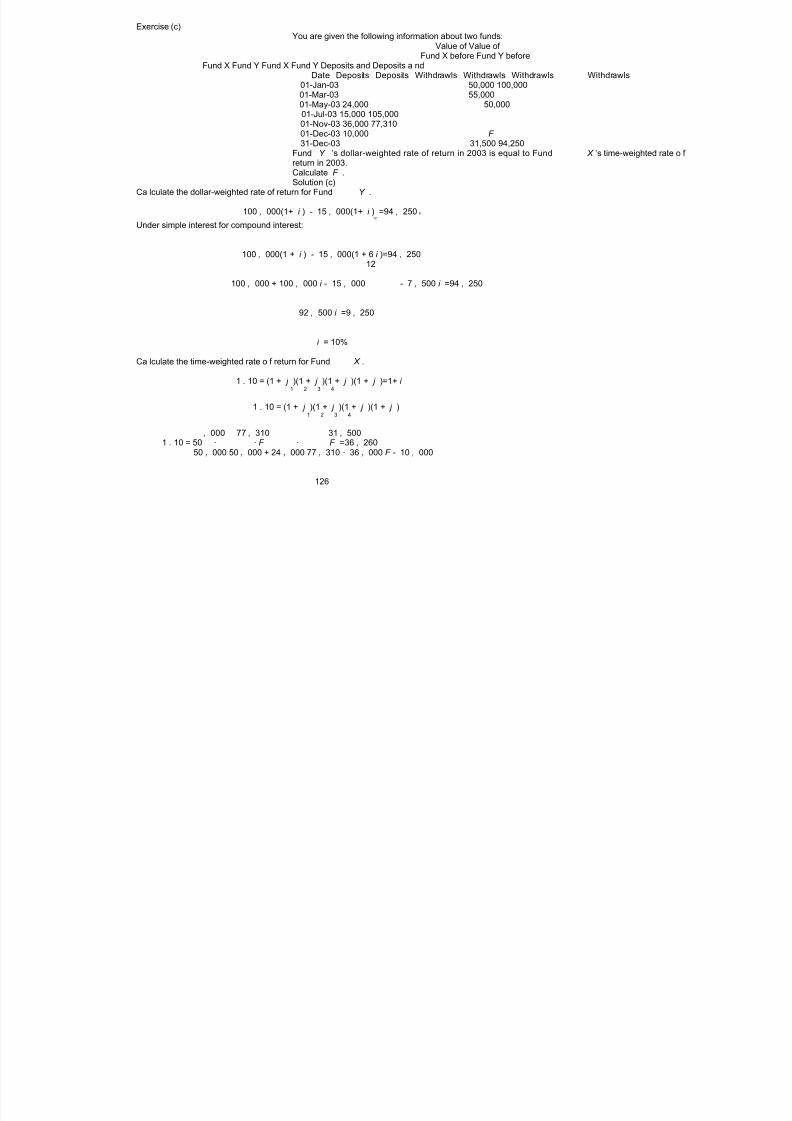
8/8/2019 3500145 Financial Math for Actuary and Businessman
http://slidepdf.com/reader/full/3500145-financial-math-for-actuary-and-businessman 128/181
Exercise (c)You are given the following information about two funds:
Value of Value of Fund X before Fund Y before
Fund X Fund Y Fund X Fund Y Deposits and Deposits a ndDate Deposits Deposits Withdrawls Withdrawls Withdrawls Withdrawls
01-Jan-03 50,000 100,00001-Mar-03 55,00001-May-03 24,000 50,00001-Jul-03 15,000 105,00001-Nov-03 36,000 77,31001-Dec-03 10,000 F 31-Dec-03 31,500 94,250
Fund Y ’s dollar-weighted rate of return in 2003 is equal to Fund X ’s time-weighted rate o f return in 2003.Calculate F .Solution (c)
Ca lculate the dollar-weighted rate of return for Fund Y .
100 , 000(1+ i ) - 15 , 000(1+ i ) =94 , 250 6
12
Under simple interest for compound interest:
100 , 000(1 + i ) - 15 , 000(1 + 6 i )=94 , 25012
100 , 000 + 100 , 000 i - 15 , 000 - 7 , 500 i =94 , 250
92 , 500 i =9 , 250
i = 10%
Ca lculate the time-weighted rate o f return for Fund X .
1 . 10 = (1 + j )(1 + j )(1 + j )(1 + j )=1+ i
1 2 3 4
1 . 10 = (1 + j )(1 + j )(1 + j )(1 + j )1 2 3 4
, 000 77 , 310 31 , 5001 . 10 = 50 · · F · F =36 , 260
50 , 000 50 , 000 + 24 , 000 77 , 310 - 36 , 000 F - 10 , 000
126

8/8/2019 3500145 Financial Math for Actuary and Businessman
http://slidepdf.com/reader/full/3500145-financial-math-for-actuary-and-businessman 129/181
5.4 Allocating Investment Income
Exercise (a)The following table shows the annual e ective interest rates being credited in an investmentaccount, by the calendar year of the investment. The investment year metho d is applicable
for the first three years, after which a portfolio rate is used:Calendar Year Investment Yea r Rates Calendar Year Portf olio
of Investment i i i of Portfolio Rate Rate1 2 3
1996 12% 12% t% 1999 8%1997 12% 5% 10% 2000 ( t - 1)%1998 8% ( t - . 02)% 12% 2001 6%1999 9% 11% 6% 2002 9%2000 7% 7% 10% 2003 10%
An investment of 100 is made at the beginning of years 1996, 1997 and 1998. The total
amount of interest credited by the fund during 1999 is equal to 28.49. Calculate t .Solution (a)
Interest earned in 1999 is equal to the 1999 interest rate multiplied by the balance at January01, 1999.
1996 Money
100(1 . 12)(1 . 12 )(1 + t )(8%)
1997 Money
100(1 . 12)(1 . 05)(10%) = 11 . 76
1998 Money
100(1 . 08)( t - . 02) = 108( t - . 02)
Total Interest = 10 . 0353(1 + t )+11 . 76 + 108( t - . 02) = 28 . 49
t =7 . 5%
127
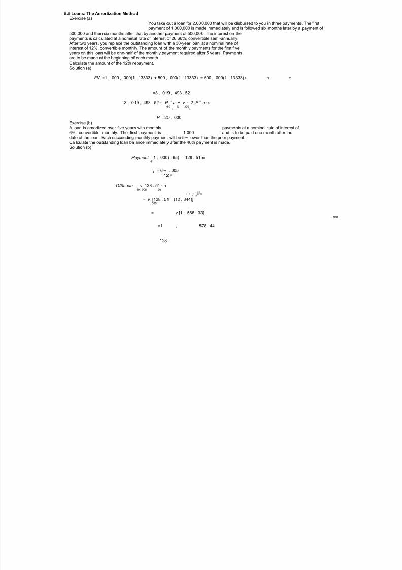
8/8/2019 3500145 Financial Math for Actuary and Businessman
http://slidepdf.com/reader/full/3500145-financial-math-for-actuary-and-businessman 130/181
5.5 Loans: The Amortization MethodExercise (a)
You take out a loan for 2,000,000 that will be disbursed to you in three payments. The firstpayment of 1,000,000 is made immediately and is followed six months later by a payment of
500,000 and then six months after that by another payment of 500,000. The interest on thepayments is calculated at a nominal rate of interest of 26.66%, convertible semi-annually.After two years, you replace the outstanding loan with a 30-year loan at a nominal rate of interest of 12%, convertible monthly. The amount of the monthly payments for the first fiveyears on this loan will be one-half of the monthly payment required after 5 years. Paymentsare to be made at the beginning of each month.Calculate the amount of the 12th repayment.Solution (a)
FV =1 , 000 , 000(1 . 13333) + 500 , 000(1 . 13333) + 500 , 000(1 . 13333) 4 3 2
=3 , 019 , 493 . 52
3 , 019 , 493 . 52 = P ¨ a + v · 2 P ¨ a 6 060 1% 300
1 % 1 %
P =20 , 000Exercise (b)A loan is amortized over five years with monthly payments at a nominal rate of interest of 6%, convertible monthly. The first payment is 1,000 and is to be paid one month after thedate of the loan. Each succeeding monthly payment will be 5% lower than the prior payment.Ca lculate the outstanding loan balance immediately after the 40th payment is made.Solution (b)
Payment =1 , 000( . 95) = 128 . 51 4041
j = 6% . 00512 =
O/SLoan = v 128 . 51 · a40 . 005 20
. 00 5i = 1 + - 1= . 057 89
1 - . 95
= v [128 . 51 · (12 . 344)]. 005
= v [1 , 586 . 33]. 005
=1 , 578 . 44
128

8/8/2019 3500145 Financial Math for Actuary and Businessman
http://slidepdf.com/reader/full/3500145-financial-math-for-actuary-and-businessman 131/181
Exercise (c)You borrow 1,000 at an annual e ective interest rate of 4% and agree to repay it with 3annual installments. The amount of each payment in the last 2 years is set at twice that
in the first year. At the end of 1 year, you have the option to repay the entire loan with afinal payment of X , in addition to the regular payment. This will yield the lender an annuale ective rate of 4.5% over the 1-year period.Solution (c)
, 0001 , 000 = P · v +2 P ( v + v ) P = 1 . 93 1 2 3
v +2( v + v ) = 217 4% 4% 4% 1 2 34% 4% 4%
, 000 -(217 . 93) · v 1
4 . 5% 1 , 000 = (217 . 93) · v + Xv X = 1 = 827 . 07 1 1
4 . 5% 4 . 5% v 14 . 5%
Exercise (d)
A loan is to be repaid by annual installments of P at the end of each year for 10 years. Youare given:
(i) The total principal repaid in the first 3 years is 290.35.(ii) The total principal repaid in the last 3 years is 408.55.
Determine the total amount of interest paid during the life of the loan.Solution (d)
290 . 35 = Pv + Pv + Pv = Pv ( v + v + v ) 10 9 8 7 3 4 5
408 . 55 = Pv + Pv + Pv = P ( v + v + v ) 3 4 5 3 4 5
Dividing the 2 equations
290 . 35v i =5% 7
408 . 55 =
. 55P = 408 = 150 . 03
v + v + v 3 4 55 % 5% 5%
L = P · a =1 , 158 . 4410 %
5
Total Interest Paid=Tota l Payments- Loan = 10(150 . 03) - 1 , 158 . 44 = 341 . 76
129

8/8/2019 3500145 Financial Math for Actuary and Businessman
http://slidepdf.com/reader/full/3500145-financial-math-for-actuary-and-businessman 132/181
5.6 Loans: The Sinking Fund MethodExercise (a)
An investor wishes to take out a loan at an annual e ective interest rate of 9% and thenbuy a 10-year annuity whose present value is 1,000 calculated at an annual e ective interestrate of 8%. The loan is to be repaid over the next 10 years with annual end-of-year interest
payments. Annual end-of-year sinking fund deposits are also to be made that are credited atan annual e ective interest rate of 7%.Solution (a)
, 000Annual annuity payment is 1 = 149 . 03
a10
8 %
The annuity payment must cover the interest payment and the sinking fund deposit.
Price149 . 03 = + Price· 9%
s 107%
. 03Price = 149 . 80
+9% = 917 1s
107%
Exercise (b)A 5% 10-year loan of 10,000 is to be paid by the sinking fund method, with interest andsinking fund payments made at the end of each year. The e ective rate of interest earned inthe sinking fund is 3% per annum.
Immediately before the fifth payment is due, the lender requests that the loan be repaidimmediately.Ca lculate the net amount of the lo an at that time.Solution (b)
, 000Sinking fund deposit is 10 = 872 . 30
s10
3%
Sinking fund balance just before the fifth deposit is to be made is 892 . 30 s (1 . 03) = 3 , 758 . 864
3 %
Value of the loan just before the interest payment is due is 10 , 000(1 . 05) = 10 , 500
Net amount of the loan at time 5 is the value of the loan less the sinking fund balance is
10 , 500 - 3 , 786 . 86 = 6 , 741 . 14
130

8/8/2019 3500145 Financial Math for Actuary and Businessman
http://slidepdf.com/reader/full/3500145-financial-math-for-actuary-and-businessman 133/181
Exercise (c)You borrow 10,000 for 10 years at an annual e ective interest rate of i a nd accumulate theamount necessary to repay the lo an by using a sinking fund. Ten payments of X are made
at the end of each year, which includes interest on the loan and the payment into the sinkingfund, which earns an annual e ective rate of 8%.If the annual e ective rate of the loan ha d been 2 i , your total annual payment would havebeen 1 . 5 X .Calculate i .Solution (c)
, 000X = i · 10 , 000 + 10
s10
8%
, 0001 . 5 X =2 i · 10 , 000 + 10
s10
8 %
0 . 5 X = i · 10 , 000 X =2 i · 10 , 000
, 0002 i · 10 , 000 = i · 10 , 000 + 10
s10
8%
. 29i = 690 . 9%
10 , 000 =6
131

8/8/2019 3500145 Financial Math for Actuary and Businessman
http://slidepdf.com/reader/full/3500145-financial-math-for-actuary-and-businessman 134/181
6 Financial InstrumentsOverview
– interest theory is used to evaluate the prices and values of:1. bonds2. equity (common stock, preferred stock)
– this chapter will show how to:1. calculate the price of a security, given a yield rate2. ca lculate the yield rate of a security, give the price
6.1 Types of Financial InstrumentsThere are seven types of common securities available in the financial markets that are discussedin this chapter:
6.1.1 Money Market Instruments – provide high liquidity and attractive yields; some allow cheque writing
– contains a variety of short-term, fixed-income securities issued by governments and priva tefirms – credited rates uctuate frequently with movements in short-term interest ra tes – investors will ”park” their money in an MMF while contemplating their investment options
Treasury Bills (T-bills) – Government issued bonds are called:
- Treasury Bills (if less than one year)- Treasury Notes (if in between one yea r and long-term)- Treasury Bonds (if long-term)
– Treasury Bills are valued on a discount yield basis using actual/360Question: Find the price of a 13-week T-bill that matures for 10 , 000 and is bought at discountto yield 7 . 5%.Solution:
9110 , 000 1 - . 5%) =9 , 810 . 42
360(7
Certificate of Deposits (CD) – rates are guaranteed for a fixed period of time ranging from 30 days to 6 months – higher denominations will usually credit higher rates of interest
– yield rates are usually more stable than MMF’s but less liquid – withdrawal penalties tend to encourage a secondary trading market rather than cashingout
132

8/8/2019 3500145 Financial Math for Actuary and Businessman
http://slidepdf.com/reader/full/3500145-financial-math-for-actuary-and-businessman 135/181
Commercial Paper – is an unsecured debt note that usually lasts one to two months, up to 270 days – usually issued by a large corporation – the face amount is most likely in multiples of $100,000
6.1.2 Bonds – promise to pay interest over a specific term a t stated future dates and then pay lump sum
at the end of the term (similar qualities to an amortized loan approach). – issued by corporations and governments as a way to raise money (i.e. borrowing). – the end of the term is called a maturity date; some bonds can be repaid at the discretion of
the bond issuer at any redemption date (callable bonds). – interest payments from bonds are called coupon payments. – bonds without coupons and that pay out a lump sum in the future are called accumulation
bonds or zero-coupon bonds. – a bo nd that has a fixed interest rate over the term of the bond is called fixed-rate bonds. – a bo nd that has a uctuated interest rate over the term of the bond is called a oating-ra te
bond.
– the risk that a bond issuer do es not pay the coupon or principal payments is called defaultrisk. – a mortgage bond is a bond backed by collateral; in this case, by a mortgage on real property
(more secure) – an income bond pays coupons if company had su cient funds; no threat of bankruptcy for
missedcouponpayment – junk bonds have a high risk of defaulting on payments and therefore need to o er higher
interest rates to encourage investment – a convertible bond can be converted into the common stock of the company at the option o f
the bond owner – borrowers in need of a large amount money may choose to issue serial bonds that have
staggered maturity dates
6.1.3 Common Stock – is an ownership security, like preferred stock, but do es not have fixed dividends – level of dividend is determined by company’s directors – commo n stock dividends are paid after interest payments for bonds and preferred stock are
paid out – variable dividend rates means prices are more volatile than bonds and preferred stock
133

8/8/2019 3500145 Financial Math for Actuary and Businessman
http://slidepdf.com/reader/full/3500145-financial-math-for-actuary-and-businessman 136/181
6.1.4 Preferred Stock – provides a fixed rate o f return (similar to bonds); called a dividend – ownership of sto ck means ownership of company (not borrowing) – no maturity date – for creditor purpose, preferred sto ck is second in line, behind bond owners (common sto ck is
third) – failure to pay dividend does not result in default – cumulative preferred stock will make up for any missed dividends; reg ular preferred stock
does not have to – convertible preferred sto ck gives the owner the option of converting to common stock under
certain conditions
6.1.5 Mutual Funds – pooled investment accounts; an investo r buys shares in the fund – o ers more diversification than what an individual can achieve on their own – a money manager controls the investment; if the money manager trys to outbeat the market
it is said that the investment stra tegy is active, if the money manag er matches the index
fund then the investment strategy is passive.
6.1.6 G uaranteed Investment Contracts (G IC) – issued by insurance companies to large investors – similar to CD’s; market value does not change with interest rate movements – GIC might allow for additional deposits and can o er insurance contract features i.e. annuity
purchase options – interest rates higher than CD’s; closer to Treasury securities – banks compete with their “bank investment contracts” (BIC)
134

8/8/2019 3500145 Financial Math for Actuary and Businessman
http://slidepdf.com/reader/full/3500145-financial-math-for-actuary-and-businessman 137/181
6.1.7 Derivative Sercurities – the value of a derivative security depends on the value of the underlying asset in the market-
place
Options – a contract that allows the owner to buy or sell a security at a fixed price at a f uture da te – call option gives the owner the right to buy; put option gives the owner the right to sell – European option can be used on a fixed date; American option can be used any time until
its expiry date – investors will buy(sell) call options or sell(buy) put options if they think a security’s price is
going to rise (fall) – one motivation for buying or selling options is speculation; option prices depend on the value
of the underlying asset (leverage) – another motiva tion (and quite opposite to speculation) is developing hedging strategies to
reduce investment risk (see Section 8 . 7 Short Sales) – a warrant is similar to a call option, but has more distinct expiry dates; the issuing firm also
has to own the underlying security
– a convertible bond may be considered the combination of a regular bond and a warrantFut ur es – this is a contract where the investor agrees, at issue, to buy or sell an asset at a fixed date
(delivery date) at a fixed price (f utures price) – the current price o f the asset is called the spo t price – an investor has two investment alternatives:
(i) buy the asset immediately and pay the spot price now, or
(ii) buy a futures contract and pay the futures price at the delivery date; earn interest onthe money deferred, but lose the opportunity to receive dividends/interest payments
For wa r ds – similar to futures except that forwards are tailored made between two parties (no active
market to trade in) – banks will buy and sell forwards with investors who want protection for currency rate uc-
tuations for one year or longer – banks also sell futures to investors who wish to lock-in now a borrowing interest rate that
will be applied to a future loan – risk is that interest rates drop in the future and the investo r is stuck with the higher interest
rate
135

8/8/2019 3500145 Financial Math for Actuary and Businessman
http://slidepdf.com/reader/full/3500145-financial-math-for-actuary-and-businessman 138/181
Swaps – a swap is an exchange of two similar financial quantities – for example, a change in loan repayments from Canadian dollars to American dollars is called
a currency swap (risk depends on the exchange rate) – an interest rate swap is where you agree to make interest payments based on a variable loan
rate ( oating rate) instead of on a predetermined loan rate (fixed rate)Caps
– an interest rate cap places an upper limit on an interest rate to protect the investor againstincreasing interest ra tes.
Cap payment = Max index rate-strike rate 0 · notational amount p ,
where p is the amount of times per year interest is paidFloors
– an interest rate oor a lower limit on an interest rate to protect the investor against decreasing
interest rates.
Floor payment = Max strike rate-index rate 0 · notational amount p ,
where p is the amount of times per year interest is paid
136

8/8/2019 3500145 Financial Math for Actuary and Businessman
http://slidepdf.com/reader/full/3500145-financial-math-for-actuary-and-businessman 139/181
6.2 Bond Valuation – like any loan, the price(value) of a bond can be determined by taking the present value of its
future payments – prices will be calculated immediately after a coupon payment has been made, or alternatively,
at issue date if the bond is bra nd new –let P represent the price of a bond that o ers coupon payments of ( Fr ) and a final lump
sum payment of C . The present value is calculated as follows:
P =( Fr ) · a + Cv nn i
i
– F represents the face amount(par value) of a bond. It is used to define the coupon paymentsthat are to be made by the bond.
– C represents the redemption value of a bond. This is the amount tha t is returned to thebond-holder(lender) at the end of the bond’s term (i.e. at the maturity date).
– r represents the coupon rate of a bond. This is used with F to define the bond’s couponpayments. This ”interest rate” is usually quoted first on a no minal basis, convertible semi-annually since the coupon payments are often paid on a semi-annual basis. This interest rate
will need to be converted bef ore it can be applied. –( Fr ) represents the semi-annual cou pon payment of a bond. – n is the number of coupon payments remaining or the time until maturity. – i is the bond’s yield rate or yield-to-maturity .Itisthe IRR to the bond-holder for acquiring
this investment. Recall that the yield rate for an investment is determined by setting thepresent value of cash- ows-in (the purchase price, P ) equal to the present value of the cash-ows-out (the coupon payments, ( Fr ), and the redemption value, C ).
– there are three formulas that can be used in order to determine the price o f a bond:(i) Basic Formula
(ii) Premium/Discount Formula(iii) Base Amount Formula
(i) Basic FormulaP =( Fr ) · a + Cv n
n i i
As stated before, a bond’s price is equal to the present value of its future payments.
(ii) Premium/Discount Formula
P =( Fr ) · a + Cv n
n i i
=( Fr ) · a + C (1 - i · a )n n
i i
= C +( Fr- Ci ) an
i
If we let C loosely represent the loan amount that the bond-holder gets back, then ( Fr- Ci )represents how much better the actual payments, Fr , are relative to the ”expected” interest
137

8/8/2019 3500145 Financial Math for Actuary and Businessman
http://slidepdf.com/reader/full/3500145-financial-math-for-actuary-and-businessman 140/181
payments, Ci .
When ( Fr- Ci ) > 0 the bond will pay out a ”superior” interest payment than what the yieldrate says to expect. As a result, the bond-buyer is willing to pay(lend) a bit more, P - C ,than what will be returned at maturity. This extra amount is referred to as a ”premium”.On the other hand, if the coupo n payments are less than what is expected according to theyield rate, ( Fr- Ci ) < 0, then the bond-buyer won’t buy the bond unless it is o ered at aprice less than C or, in other words, at a ”discount”.
(iii) Base Amount Formula
Let G represent the base amount of the bond such that if multiplied by the yield rate, itwould produce the same coupon payments that the bond is providing: Gi = Fr G = . Fr
i
The price of the bond is then calculated as follows:
P =( Fr ) · a + Cv nn i
i
=( Gi ) · a + C (1 - i · a )n n
i i
= G · (1 - v )+ Cv n n
i i
n = G +( C - G ) v i
If we now let G loosely represent the loan, then the amount that the bond-holder receivesat maturity, in excess of the loan, would be a bonus. As a result, the bond becomes morevaluable and a bond-buyer would be willing to pay a higher price than G . On the other hand, if the payout at maturity is perceived to be less than the loan G , then the bond-buyer will not purchase the bond unless the price is less than the loan amount.
Determination Of Yield Rates – given a purchase price of a security, the yield rate can be determined under a number of
methods.Problem:
What is the yield rate convertible semi-annually for a 100 par value 10-year bond with 8%semi-annual coupons that is currently selling for 90?
Solution:1. Use an Society of Actuaries recommended calculator with built in financial functions:
PV =90 , N =2 × 10 = 20 , FV = 100 , PMT = 8% × 100 = 4 ,2
CPT %i 4 . 788% × 2=9 . 5676%
2. Do a linear interpolation with bond tables (not a very popular method anymore).
138
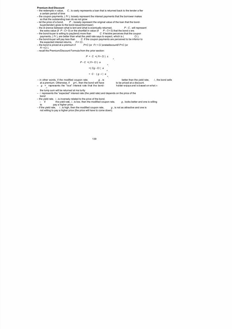
8/8/2019 3500145 Financial Math for Actuary and Businessman
http://slidepdf.com/reader/full/3500145-financial-math-for-actuary-and-businessman 141/181
Premium And Discount – the redemptio n value, C , lo osely represents a loan that is returned back to the lender a fter
a certain period of time – the coupon payments, ( Fr ), loosely represent the interest payments that the borrower makes
so that the outstanding loan do es not grow – let the price of a bond, P , loosely represent the original value of the loan that the bond-
buyer(lender) gives to the bond-issuer(borrower) – the di erence between what is lent and what is eventually returned, P - C , will represent
the extra value (if P - C> 0) or the shortfall in value (if P - C< 0) that the bond o ers – the bond-buyer is willing to pay(lend) more than C if he/she perceives that the coupon
payments, ( Fr ), are better than what the yield rate says to expect, which is ( Ci ). – the bond-buyer will pay less than C if the coupon payments are perceived to be inferior to
the expected interest returns, Fr< Ci . – the bond is priced at a premium if P>C (or Fr > Ci )oratadiscountif P<C (or
Fr <Ci ). – recall the Premium/Discount Formula from the prior section:
P = C +( Fr- Ci ) a ni
P - C =( Fr- Ci ) an
i
=( Cg - Ci ) an
i
= C · ( g - i ) an
i
– in other words, if the modified coupon rate, g , is better than the yield rate, i , the bond sellsat a premium. Otherwise, if g<i , then the bond will have to be priced at a discount.
– g = represents the ”true” interest rate that the bond- holder enjoys and is based on what Fr
C
the lump sum will be returned at ma turity – i represents the ”expected” interest rate (the yield rate) and depends on the price of the
bond – the yield rate, i , is inversely related to the price of the bond. – if the yield rate, i , is low, then the modified coupon rate, g , looks better and one is willing
to pay a higher price. – if the yield rate, i , is high, then the modified coupon rate, g , is not as attractive and one is
not willing to pay a higher price (the price will have to come down).
139

8/8/2019 3500145 Financial Math for Actuary and Businessman
http://slidepdf.com/reader/full/3500145-financial-math-for-actuary-and-businessman 142/181
Example
Letthereexistabondsuchthat C = 1. The co upon payments are therefore equal tog ( Fr = Cg = g ).
Let the price of the bond be denoted as 1 + p where p is the premium (if p> 0) or thediscount (if p< 0).
P =( Fr ) · a + Cv nn i
i
n 1+ p = g · a+(1) v
n i i
= g · a +1 - i · an n
i i
=1+( g - i ) · an
i
Amortization of Premium and Accrual of Discount
Interest Earned: I t
– using the pro spective method for evaluating the value (current price) of the bond, the interestpayment is derived as follows:
I = i · BV t t- 1
n - ( t- 1) = i g · a +(1) v n - ( t - 1) i
i
n - ( t- 1 ) n - ( t- 1) = g · 1 - v + v i i
n - ( t- 1) = g - ( g - i ) · v i
– therefore, each coupon payment, g , is intended to represent a periodic interest paymentplus(less) a return of portion o f the premium(discount) that was made at purchase.
n - ( t - 1) I = g - ( g - i ) · v t i
n - ( t- 1) g = I +( g - i ) · v t i
Premium Amortization: PAt
– the premium amortization in this case is equal to the coupon payment less the interestpayment, g - I :
t
PA = g - I t t
n - ( t- 1) = g - [ g - ( g - i ) · v ]i
n - ( t- 1) PA =( g - i ) · v t i
Other Premium Amortization Formulas
PA = BV - BV t t- 1 t
Amortization of Premium over the t-th perio d= PAt
Accumulation of Discount over the t-th perio d= -PAt
140

8/8/2019 3500145 Financial Math for Actuary and Businessman
http://slidepdf.com/reader/full/3500145-financial-math-for-actuary-and-businessman 143/181
Bo ok Value Of The Bond – the bond’s value starts at price P (or 1 + p , in our example) and eventually, it will become
value C (or 1, in our example) at maturity. – this value, or current price of the bond, at any time between issue date and maturity date
can be determined using the prospective approach:
BV =( Fr ) · a + Cv n -t
t n - t i i
n - t 1+ p = g ·a +(1) v
n - t i i
= g · a +1 - i · an - t n - t
i i
=1+( g - i ) · an - t
i
– or it can be determined using the retro spective approach:
BV = P (1 + i ) - Frs t t t
i
= P (1 + i ) - Cgs t
t i
– when this asset is first acquired by the bond-buyer, its value is recorded into the accountingrecords, or the ”boo ks”, at its purchase price. Since it is assumed that the bond will now beheld until maturity, the bond’s future value will continue to be calculated using the originalexpected rate of return (the yield rate that was used at purchase).
– the current value of the bond is often referred to as a ”bo ok value”. – the value of the bond will eventually drop or rise to value C depending if it was originally
purchased at a premium or at a discount.f
Book Value Formulas
n -t BV = Cga + Cv t n - t t
i
= P (1 + t ) + Cgs t
t i
= BV (1 + i ) - Cg t- 1
= BV + I - Cg t- 1 t
= BV - PAt- 1 t
= BV - Amortization of Premiumt- 1
= BV + Accumulation of discount t- 1
141

8/8/2019 3500145 Financial Math for Actuary and Businessman
http://slidepdf.com/reader/full/3500145-financial-math-for-actuary-and-businessman 144/181
Bond Amortization Schedule – an amortization schedule for this type of loan can also be developed that will show how the
bond is being written down , if it was purchased at a premium, or how it is being written up ,if it was purchased at a discount.
– the following bond amortization schedule illustrates the progression of the coupon paymentswhen C = 1 and when the original price of the bond was 1 + p =1+( g - i ) · a :
ni
Period ( t ) Co upon Interest Earned I Amorization of Premium PA Book Value BV t t t
1 gg- ( g - i ) · v ( g - i ) · v 1+( g - i ) · a n n
i i n - 1i
2 gg- ( g - i ) · v ( g - i ) · v 1+( g - i ) · a n - 1 n - 1i i n - 2
i
.
. . . . .
. . . . . . . . .
n - ( t- 1) n - ( t- 1 ) tgg- ( g - i ) · v ( g - i ) · v 1+( g - i ) · a
n - t i i i
. . . . . .
. . . . . . . . .
n - 1 gg- ( g - i ) · v ( g - i ) · v 1+( g - i ) · a 2 2i i 1
i
ngg- ( g - i ) · v ( g - i ) · v 1 1i i
Total n · gn· g - ( g - i ) a ( g - i ) · a = pn n
i i
142

8/8/2019 3500145 Financial Math for Actuary and Businessman
http://slidepdf.com/reader/full/3500145-financial-math-for-actuary-and-businessman 145/181
– note that the total of all the interest payments is represented by the total of all couponpayments less what is being returned as the premium (or plus what is being removed asdiscount since the loan is appreciating to C ).
n n
n - ( t- 1) I = g - ( g - i ) · v k i
k = 1 k = 1n n
n - ( k - 1) = g - ( g - i ) · v i
k = 1 k = 1
= ng - ( g - i ) an
i
= ng - p
– note that the total of all the principal payments must equal the premium/discount
n n
n - ( k - 1) P = ( g - i ) v =( g - i ) a = pk n i i
k = 1 k = 1
– note that the book value at t = n is equal to 1, the last and final payment back to thebond-holder.
– note that the principal (premium) repayments increase geometrically by 1+ i ( 2)
2
n
i.e. PA = PA 1+ . i ( 2)
t + n t 2
– remember that the above exa mple is based on a redemptio n value of C =1. Theaboveformulas need to be multiplied by the actual redemption value if C is not equal to 1
143

8/8/2019 3500145 Financial Math for Actuary and Businessman
http://slidepdf.com/reader/full/3500145-financial-math-for-actuary-and-businessman 146/181
Straight Line Method
If an approximation for writing up or writing down the bond is acceptable, then the principalpayments can be defined as follows:
BV - BV 0 n PA =
t n . p - 1 p
or PA = 1+ = ,if C =1.t n n
I will then be the coupon payment less the premium amortization:t
- BV 0 n I =( Cg
) - PA =( Cg ) - BV t t n .
or I = g - p ,if C =1.t n
The book value of the bond, BV , will then be equal the original price less the sum of thet
premium repayments made to date:
t - BV 0 n BV = BV - PA = BV - t BV = BV - tP A .
t 0 k 0 0 t nk = 1
n - t or Price =1+ p - t p =1+ ,if C =1.
t n n p
144

8/8/2019 3500145 Financial Math for Actuary and Businessman
http://slidepdf.com/reader/full/3500145-financial-math-for-actuary-and-businessman 147/181
The bond amortization table would then be developed as follows:
Period ( t )Payment I P Book Valuet t t
1 gg- 1+ p p p n - 1n n n
2 gg- 1+ p p p n - 2n n n
.
. . . . .
. . . . . . . . .
tgg- 1+ p p p n -t
n n n
.
. . . . . . . . . . . . . .
p p n - 1 gg-1+ p 1n n n
ngg- 1 p p
n n
Total ng ng - p · n = p p
n
Callable Bonds – this is a bond where the issuer can redeem the bond prior to the maturity date if they so
chooseto;thisiscalleda call date . – the challenge in pricing callable bonds is trying to determine the most likely call date – assuming that the redemption date is the same at any call date, then
(i) the call date will most likely be at the earliest date possible if the bond was sold at a
premium (issuer would like to stop repaying the premium via the coupon payments assoon as possible).(ii) the call date will most likely be at the latest date possible if the bond was sold at a
discount (issuer is in no rush to pay out the redeption value). – when the redemption date is not the same at every ca ll date, then one needs to examine all
possible call dates.
145
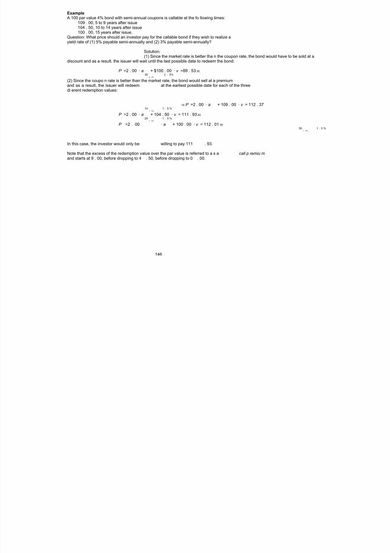
8/8/2019 3500145 Financial Math for Actuary and Businessman
http://slidepdf.com/reader/full/3500145-financial-math-for-actuary-and-businessman 148/181
ExampleA 100 par value 4% bond with semi-annual coupons is callable at the fo llowing times:
109 . 00, 5 to 9 years after issue104 . 50, 10 to 14 years after issue100 . 00, 15 years after issue.
Question: What price should an investor pay for the callable bond if they wish to realize ayield rate of (1) 5% payable semi-annually and (2) 3% payable semi-annually?
Solution:(1) Since the market rate is better tha n the coupon rate, the bond would have to be sold at a
discount and as a result, the issuer will wait until the last possible date to redeem the bond:
P =2 . 00 · a + $100 . 00 · v =89 . 53 3030 2 . 5%
2 . 5%
(2) Since the coupo n rate is better than the market rate, the bond would sell at a premiumand as a result, the issuer will redeem at the earliest possible date for each of the threedi erent redemption values:
10 P =2 . 00 · a + 109 . 00 · v = 112 . 3710 1 . 5 %
1 . 5%
P =2 . 00 · a + 104 . 50 · v = 111 . 93 2020 1 . 5 %
1 . 5%
P =2 . 00 · a + 100 . 00 · v = 112 . 01 3030 1 . 5 %
1 . 5%
In this case, the investor would only be willing to pay 111 . 93.
Note that the excess of the redemption value over the par value is referred to a s a call p remiu mand starts at 9 . 00, before dropping to 4 . 50, before dropping to 0 . 00.
146

8/8/2019 3500145 Financial Math for Actuary and Businessman
http://slidepdf.com/reader/full/3500145-financial-math-for-actuary-and-businessman 149/181
Bond Price Between Coupon Payment Dates – up to now, bond prices and book values have been calculated assuming the coupon has just
been paid. –let P be the bond price (book value) just after a coupon payment has been made.
t
P = Fr.a + Cv = B (1 + i ) - Fr n - t
t t- 1 n - t i i
– when buying an existing bond between its coupon dates, one must decide how to split upthe coupon between the prior owner and the new owner.
–let Fr represent the amount of coupon (accrued coupon) that the prior owner is due wherek
0 <k< 1 – the price of the bond (full price) to be paid to the prio r owner at time t + k should be based
on the clean price of the bond and the accrued interest (accrued coupon)P = Clea n Pri ce + Accrued Interest
t + k
Accrued Interest – notice that the clea n price of the bond, will only recognize future coupon payments; hence,
the reason for a separate calculation to account for the accrued coupon, Fr .k
– k maybecalculatedonan actual/actual or 30 / 360basisifdaysaretobeused.
AI = coupon · k = Fr· k
the number of days between the last coupon payment date and settlement datewhere k =
total number days between coupon payment datesFull Price between Coupon Payments Dates
– full price is equal to the bond value as at the last coupon payment date, carried forward withcompound interest.
– or the full price is equal to the sum of the next coupon Fr , and the price of the next couponP , a ll discounted back to the settlement date.
t + 1
P = P (1 + i ) k
t + k t
= P t + k
(1 -k ) =( P + Fr ) v t + 1 i
Clean Price of Bond between Coupon Payment Dates
Clean price = P - AI t + k
= P (1 + i ) - ( coupon · k ) k
t
= P (1 + i ) - ( Fr· k ) k
t
147

8/8/2019 3500145 Financial Math for Actuary and Businessman
http://slidepdf.com/reader/full/3500145-financial-math-for-actuary-and-businessman 150/181
6.3 Stock ValuationCommon Stock
– issued by corporations i.e. borrowing, but not paying back the principal. – pays out annually a dividend, Div , rather than interest with no requirement to guarantee
payments. Also the dividend can be in any amount (not fixed income). – an assumption is required with respect to the annual growth rate of dividends, k . – Price is equal to the present value of future dividends at a given yield rate r and as given
growth rate, g .General DCF Stock Valuation Formula
8 div t PVstock =
(1 + r ) t
t = 1
Level Dividend Stock Valuation Formula
div
1 PVstock =r
Constant Dividend Growth – the techniques to be used are exactly the same a s those methods presented in Section 3 . 6,
Compound Increasing Annuities.Div
PV = v Div · ¨ a =r 8 r - g
r r = 1+ 1
1+ g -
ExampleAssuming an annual e ective yield rate of 10%, calculate the price of a common stock thatpays a 2 annual dividend at the end of every year and grows at 5% for the first 5 years, 2 . 5%for the next 5 years and 0%, thereafter:
P = v 2 · ¨ a1 0% 5
r = 1 +10 % - 11+5 %
+ v v 2(1 + 5%) · ¨ a 5 510% 10% 5
r = 1+1 0% - 11+2 . 5%
+ v v 2(1 + 5%) (1 + 2 . 5%) · ¨ a 1 0 5 58 10% 10%
r = 1+1 0% - 11+0%
P =8 . 30 + 6 . 29 + 11 . 13 = 25 . 72
Price to Earning (P/E) ratio
stock pr ice per share P 0 P/Eratio = =
earnings per share EP S net i ncome
where earnings per share =number of outstanding shares
148

8/8/2019 3500145 Financial Math for Actuary and Businessman
http://slidepdf.com/reader/full/3500145-financial-math-for-actuary-and-businessman 151/181
Exercises and Solutions6.2 Bond Valuation
Exercise (a)Youaregiventwo n - year 1000 par value bonds. Bond X has 14% semiannual coupons anda price of 1407.70, to yield i , compo unded semiannually.Bond Y has 12% semiannual coupons and a price of 1271.80, to yield the same rate i ,
compounded semiannually. Calculate the price o f Bond X to yield i - 1%.Solution (a)
1 , 407 . 70 = 1 , 000 + 1 , 000 7% - i a . 40770 = 7% - i a2 2 2 n 2 n
i i 2 2
1 , 271 . 80 = 1 , 000 + 1 , 000 6% - i a . 27180 = 6% - i a2 2 2 n
2 ni i
2 2
. 40770 - i
i . 04 i = . 08 . 40770 = (7% - 4%) a 2 n =20 2
. 27180 = 7% 6% - 2 = i 2 n
4 %
2
8% - 1%P =1 , 000 + 1 , 000 7% - a =1 , 497 . 43
2 208% - 1%
2
Exercise (b)A bond with a par value of 1,000 and 6% semiannual coupons is redeemable for 1,100. You
are given the following information.(i) The bond is purchased a P to yield 8%, convertible semiannually.
(ii) The amount of the discount adjustment from the 16th coupon payment is 5.Calculate P .Solution (b)
Fr- iBV = - 5 30 - (4%) BV = - 5 BV = 8751 5 15 15
BV = P (1 + i ) - Fr· s 1 515 15
i
875 = P (1 . 04) - 30 s 1515
4%
P = 819 . 41
149

8/8/2019 3500145 Financial Math for Actuary and Businessman
http://slidepdf.com/reader/full/3500145-financial-math-for-actuary-and-businessman 152/181
Exercise (c)A 700 par value five-year bond with 10% semiannual coupons is purchased for 670.60.The present value of the redemption value is 372.05.
Ca lculate the redemption value.Solution (c)
P = K + Fran
i
P - K = Fr· an
i
670 . 60 - 372 . 05 = 35 a = 298 . 55 i =3%10
i
372 . 05 = C · v C = 500 103%
Exercise (d)You buy an n - year 1,000 par value bond with 6.5% annual coupons at a price of 825.44,assuming an annual yield rate of i , i> 0.After the first two years, the bond’s book value has changed by 23.76. Calculate i .Solution (d)
BV - BV = BV (1 + i ) - Fr (1 + i ) - Fr- BV 22 0 0 0
23 . 76 = 825 . 44(1 + i ) - 65(1 + i ) - 65 - 825 . 44 2
0 = 825 . 44 (1 + i ) - 65 (1 + i ) - 914 . 20 2
a c b
- ( - 65) + (65) - 4(825 . 44)( - 914 . 20) 2
1+ i = . 0925 i =9 . 25%2(825 . 44) =1
150
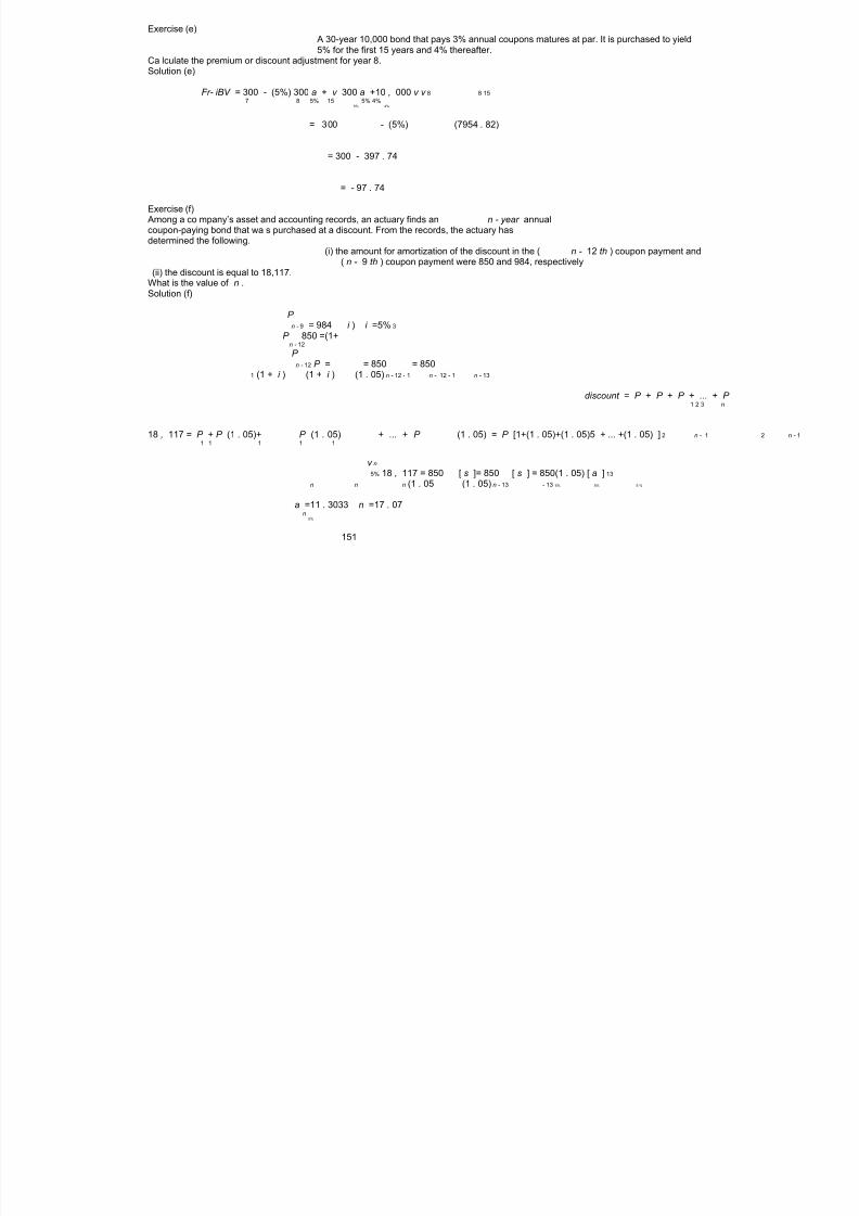
8/8/2019 3500145 Financial Math for Actuary and Businessman
http://slidepdf.com/reader/full/3500145-financial-math-for-actuary-and-businessman 153/181
Exercise (e)A 30-year 10,000 bond that pays 3% annual coupons matures at par. It is purchased to yield5% for the first 15 years and 4% thereafter.
Ca lculate the premium or discount adjustment for year 8.Solution (e)
Fr- iBV = 300 - (5%) 300 a + v 300 a +10 , 000 v v 8 8 157 8 5% 15 5% 4%
5% 4%
= 300 - (5%) (7954 . 82)
= 300 - 397 . 74
= - 97 . 74
Exercise (f)Among a co mpany’s asset and accounting records, an actuary finds an n - year annualcoupon-paying bond that wa s purchased at a discount. From the records, the actuary hasdetermined the following.
(i) the amount for amortization of the discount in the ( n - 12 th ) coupon payment and( n - 9 th ) coupon payment were 850 and 984, respectively
(ii) the discount is equal to 18,117.What is the value of n .Solution (f)
P n - 9 = 984 i ) i =5% 3
P 850 =(1+n - 12
P n - 12 P = = 850 = 850
1 (1 + i ) (1 + i ) (1 . 05) n - 12 - 1 n - 12 - 1 n - 13
discount = P + P + P + ... + P 1 2 3 n
18 , 117 = P + P (1 . 05)+ P (1 . 05) + ... + P (1 . 05) = P [1+(1 . 05)+(1 . 05)5 + ... +(1 . 05) ] 2 n - 1 2 n - 11 1 1 1 1
v n5% 18 , 117 = 850 [ s ]= 850 [ s ] = 850(1 . 05) [ a ] 13
n n n (1 . 05 (1 . 05) n - 13 - 13 5% 5% 5 %
a =11 . 3033 n =17 . 07n
5%
151

8/8/2019 3500145 Financial Math for Actuary and Businessman
http://slidepdf.com/reader/full/3500145-financial-math-for-actuary-and-businessman 154/181
Exercise (g)A par value 10-year bond with 10% annual coupons is bought at a premium to yield anannual e ective rate of 8% for the first 5 years and 6%, thereafter.
The interest portion of the 9th coupon is 12,880.Calculate the par value.Solution (g)
I =6% · BV 9 8
12 , 880 = 6% · F (10%) a + Fv 22 6%
6 %
12 , 880 = 6% · F [1 . 07335707]
F = 200 , 000
Exercise (h)A machine costs P . At the end of 10 years, it will have a salvage value of 0 . 28 P .The book value at the end of 5 years using the sinking fund method at an annual e ectiveinterest rate of 6% is X .The bo ok value at the end of 5 years using the straight line metho d is Y .
You are give n X - Y =650.92.Calculate P .
Solution (h)
( P - . 28 P )BV = P - = X
5 s · s10 5
6% 6 %
5( P - . 28 P )BV = P - Y
5 10 =
( P - . 28 P )P - = 650 . 92
5( P -. 28 P ) s · s - P -10 5 10
6% 6 %
( P - . 28 P ) 1 - s = 650 . 92 5
2 s10
P =12 , 500
152
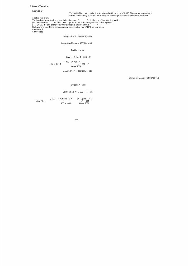
8/8/2019 3500145 Financial Math for Actuary and Businessman
http://slidepdf.com/reader/full/3500145-financial-math-for-actuary-and-businessman 155/181
6.3 Stock Valuation
Exercise (a)You and a friend each sell a di erent stock short for a price of 1,000. The margin requirementis 60% of the selling price and the interest on the margin account is credited at an annual
e ective rate of 6%.You buy back your stock one year la ter at a price of P . At the end of the year, the stockpaid a dividend of X . Your friend also buys back their stock one year later but at a price o f ( P - 25). At the end of the year, their stock paid a dividend of 2 X .Both you and your friend earn an annual e ective yield rate of 20% on your sales.Calculate P .Solution (a)
Margin (I) = 1 , 000(60%) = 600
Interest on Margin = 600(6%) = 36
Dividend = -X
Gain on Sale = 1 , 000 - P
, 000 - P +36 - X Yield (I) = 1 X = 916 - P
600 = 20%
Margin (II) = 1 , 000(60%) = 600
Interest on Margin = 600(6%) = 36
Dividend = - 2 X
Gain on Sale = 1 , 000 - ( P - 25)
, 000 - P +25+36 - 2 X - P - 2(916 - P )Yield (II) = 1 P = 891
600 = 1061 600 = 20%
153

8/8/2019 3500145 Financial Math for Actuary and Businessman
http://slidepdf.com/reader/full/3500145-financial-math-for-actuary-and-businessman 156/181
Exercise (b)You and a friend each sell a di erent stock short for a price of 1,000. The margin requirementis 50% of the selling price and the interest on the margin account is credited at an annual
e ective rate of 6%.You buy back your stock one year la ter at a price of P . At the end of the year, the stockpaid a dividend of X . Your friend also buys back their stock one year later but at a price o f ( P - 25). At the end of the year, their stock paid a dividend of 2 X .Both you and your friend earn an annual e ective yield rate of 20% on your sales.Calculate X .Solution (b)
Margin (I) = 1 , 000(50%) = 500
Interest on Margin = 500(6%) = 30
Dividend = -X
Gain on Sale = 1 , 000 - P
, 000 - P +30 - X Yield (I) = 1 X = 930 - P
500 = 20%
Margin (II) = 1 , 000(50%) = 500
Interest on Margin = 500(6%) = 30
Dividend = - 2 X
Gain on Sale = 1 , 000 - ( P - 25)
, 000 - P +25+30 - 2 X - P - 2(930 - P )Yield (II) = 1 X =25
500 = 1055 500 = 20%
154

8/8/2019 3500145 Financial Math for Actuary and Businessman
http://slidepdf.com/reader/full/3500145-financial-math-for-actuary-and-businessman 157/181
Exercise (c)A common stock is purchased on January 1, 1992. It is expected to pay a dividend of 15 per share at the end of each year throug h December 31, 2001. Starting in 2002 dividends are
expected to increase K % per year indefinitely, K< 8%. The theoretical price to yield anannual e ective rate of 8% is 200.90.Calculate K .Solution (c)
15200 . 90 = 15 a +(1 . 08) - 9
. 08 - K 98 %
K = . 01
Exercise (d)Steven buys a sto ck for 200 which pays a dividend o f 12 at the end of every 6 months. Stevendeposits the dividend payments into a bank account earning a nominal interest rate of 10%
convertible semiannually.At the end of 10 years, immediately after receiving the 20th dividend payment of 12, Steven
sells the stock. the sale price assumes a nominal yield of 8% convertible semiannually andthat the semiannual dividend of 12 will continue forever.Steven’s annual e ective yield over the 10-yea r perio d is i .Calculate i .Solution (d)
AV of dividends =12 s = 396 . 7920
5%
P = 12. 04 = 300
10 200(1 + i ) = 396 . 79 + 300
10 (1 + i ) =3 . 4840
i =13 . 29%
155

8/8/2019 3500145 Financial Math for Actuary and Businessman
http://slidepdf.com/reader/full/3500145-financial-math-for-actuary-and-businessman 158/181
7 Duration, Convexity and ImmunizationOverview
– there are two types of bond sensitivity, they are duration and convexity. – modified, Macaulay, and e ective are three types of convexity and duration. – the present value o f a company’s assets minus the present value o f a companies liabilities is
called a surplus . – when a company’s assets and liabilities are protected from interest rate uctuations, this is
called immunization . – when matching asset cash ows to liability cash ows for the protection of the surplus, this
is called dedication .
7.1 Price as a Function of Yield – examining the price curve, pr ice falls as the yield increases – price is calculated as follows:
y - m t
P = CF 1+t m
t > 0
where P =asset price, y =yield (ie. y = i )and CF =cash ow at time t years ( m )t
– the estimated percentage change in a bond’s price is approximately:
P ( y )% P ˜ ( y )
P ( y )
7.2 Modified Duration – Modified duration is calculated as follows
( y )ModD = - P
P ( y ) –where P is:
y - m t
P = CF 1+t m
- m t -tCF 1+ y dP y -m t - 1
t = -tCF 1+ = m
t dy m y 1+m
-m t dP tCF 1+ y
t dy ModD = =m
P P 1+ y
m
156

8/8/2019 3500145 Financial Math for Actuary and Businessman
http://slidepdf.com/reader/full/3500145-financial-math-for-actuary-and-businessman 159/181
Modified Duration
-m t y
tCF 1+
t ModD = t = 0 m
P 1+ y
m
Relationship between price and modified duration
% P ˜- ( y )( ModD )
where one hundred basis points equals 1.0%
7.3 Macaulay Duration – Macaulay Duration is calculated as follows:
( d ) 1MacD = - P - dP
P ( d ) = dd P
– Solving for Macaulay Duration:
P = CF e - dt
t
dP = -t · CF e - d t
t dd
1 t · CF e -d t
t MacD = - dP =dd P CF e - dt
t
- mt t · CF 1+ y t · CF e t · CF · v -d t t
t t t MacD = = = m i
P P P Relationship between Macaulay Duration and Modified Duration
MacDModD =
1+ y
m
157

8/8/2019 3500145 Financial Math for Actuary and Businessman
http://slidepdf.com/reader/full/3500145-financial-math-for-actuary-and-businessman 160/181
Example of Duration:Assuming an interest rate of 8%, calculate the duration of:(1) An n -year zero coupon bond:
n
t · v · CF t t
n · v · CF nt = n n MacD = = = n
v · CF n
nn
v · CF t t
t = n
(2) An n -year bond with 8% coupons:
n
t t · v · CF
t · ( Ia ) +10 v n
t = 1 n MacD = = 8% i i
8% · a + v n n
n i v · CF t i
t t = 1
(3) An n -year mortgage repaid with level payments of principal and interest:
n
t · v · CF t t
Ia )n t = 1 MacD = = ( i
a n
n
v · CF t i
t t = 1
(4) A preferred sto ck paying level dividends into perpetuity:
8
t · v · CF t t
Ia )t = 1 8 MacD = = (
i
a 8
8
v · CF t i
t t = 1
Macaulay Duration for Bonds Priced at Par
( m ) MacD =¨ an
i
158
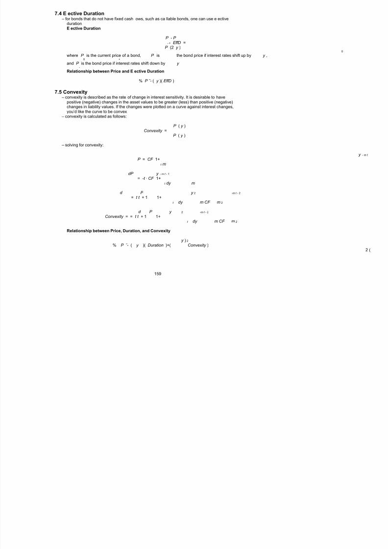
8/8/2019 3500145 Financial Math for Actuary and Businessman
http://slidepdf.com/reader/full/3500145-financial-math-for-actuary-and-businessman 161/181
7.4 E ective Duration – for bonds that do not have fixed cash ows, such as ca llable bonds, one can use e ective
durationE ective Duration
P - P - + EffD =
P (2 y )0
where P is the current price of a bond, P is the bond price if interest rates shift up by y ,0 +
and P is the bond price if interest rates shift down by y -
Relationship between Price and E ective Duration
% P ˜- ( y )( EffD )
7.5 Convexity – convexity is described as the rate of change in interest sensitivity. It is desirable to have
positive (negative) changes in the asset values to be greater (less) than positive (negative)changes in liability values. If the changes were plotted on a curve against interest changes,you’d like the curve to be convex.
– convexity is calculated as follows:
P ( y )Convexity =
P ( y )
– solving for convexity:
y - m t
P = CF 1+t m
dP y - m t - 1
= -t · CF 1+t dy m
d P y 2 -m t - 2
= t t + 1 1+t dy m CF m 2
d P y 2 -m t - 2
Convexity = = t t + 1 1+t dy m CF m 2
Relationship between Price, Duration, and Convexity
y ) 2
% P ˜- ( y )( Duration )+( Convexity )2 (
159
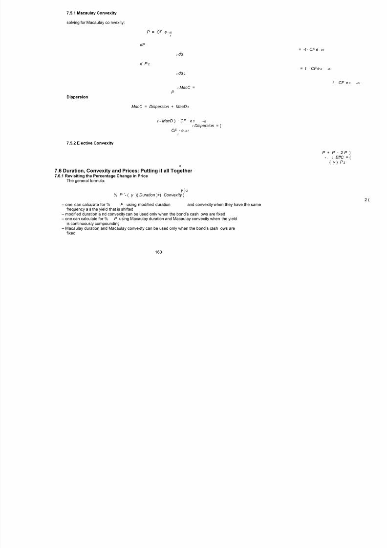
8/8/2019 3500145 Financial Math for Actuary and Businessman
http://slidepdf.com/reader/full/3500145-financial-math-for-actuary-and-businessman 162/181
7.5.1 Macaulay Convexity
solving for Macaulay co nvexity:
P = CF e - dt
t
dP = -t · CF e - d t
t dd
d P 2= t · CF e 2 -d t
t dd 2
t · CF e 2 -d t
t MacC =P
Dispersion
MacC = Dispersion + MacD 2
t - MacD ) · CF · e 2 - dt
t Dispersion = (CF · e -d t
t
7.5.2 E ective Convexity
P + P - 2 P )+ - 0 EffC = (
( y ) P 20
7.6 Duration, Convexity and Prices: Putting it all Together 7.6.1 Revisiting the Percentage Change in Price
The general formula:
y ) 2% P ˜- ( y )( Duration )+( Convexity )
2 ( – one can calculate for % P using modified duration and convexity when they have the same
frequency a s the yield that is shifted – modified duration a nd convexity can be used only when the bond’s cash ows are fixed – one can calculate for % P using Macaulay duration and Macaulay convexity when the yield
is continuously compounding – Macaulay duration and Macaulay convexity can be used only when the bond’s cash ows are
fixed
160

8/8/2019 3500145 Financial Math for Actuary and Businessman
http://slidepdf.com/reader/full/3500145-financial-math-for-actuary-and-businessman 163/181
– one can calculate for % P using e ective duration and e ective convexity when they and y have the same frequency as the yield that is shifted and when the yield is continuouslycompounding
– e ective duration and e ective convexity can be used when the bond’s cash ows are fixedand when they are not fixed
7.6.2 The Passage of Time and DurationThere are two opposite e ects that occur as a bond ages:
– duration decreases with time since the timing for each payment decreases – duration increases with time as more weight is given to the more distant cash ows (ie. it
will ”spike” as you geet closer to a cash ow)The overall e ect is that duration will decrease .
7.6.3 Portfolio Duration and ConvexityThe duration of the portfolio is:
P P P
1 2 n = D + D + ... + D1 2 n MV MV MV
po r t po r t po r t
where n is how many bonds are in the portfolio, P is the price, D is the duration andk k
MV is the market value of the portfolio po r t
The convexity of the portfolio:
P P P 1 2 n = C + C + ... + C
1 2 n MV MV MV po rt po rt po r t
where C is the bond’s convexityk
161

8/8/2019 3500145 Financial Math for Actuary and Businessman
http://slidepdf.com/reader/full/3500145-financial-math-for-actuary-and-businessman 164/181
7.7 Immunization – it is very di cult for a financial enterprise to match the cash ows of their assets to the cash
ows of their liabilities. – especially when the cash ows can change due to changes in interest rates.
Surplus
S ( y )= PV - PV A L
where y is the interest rate, PV is the present va lue of the assets and PV is the present A L
value of the liabilitiesA Problem with Interest Rates
– a bank issues a one-year deposit and guarantees a certain rate of return. – if interest rates have gone up by the end of the year, then the deposit holder will not renew
if the guaranteed rate is too low versus the new interest rate. – the bank will need to pay out to the deposit holder and if the original proceeds were invested
in long-duration assets (“going long”), then the bank needs to sell o its own assets (thathave declined in value) in order to pay.
– if interest rates have go ne down by the end of the year, then it is possible that the backingassets may not be able to meet the guaranteed rate; this becomes a greater possibility withshort-duration assets (“going short”).
– the bank may have to sell o some its assets to meet the guarantee.A Solution to the Interest Rate Problem
– structure the assets so that their cash ows move at least the same amount as the liabilities’cash ows move when interest rates change.
–let A and L represent the cash ows at time t from an institution’s assets and liabilities,t t
respectively. –let R represent the institutio n’s net cash ows at time t such that R = A - L .
t t t t n n
–if P ( i )= v · R = v · ( A - L ), then we would like the present value o f asset cash t t
t t t t = 1 t = 1
ows to equal the present value of liability cash ows i.e. P ( i )=0:
n n
v · A = v · L t t
t t t = 1 t = 1
– we’d also like the interest sensitivity (modified duration) of the asset cash ows to be equal
P ( i )to the interest sensitivity of the liabilities i.e. P ( i )=0.
P ( i ) =0
n n
t · v · A t · v · L t t
t t
t = 1 t = 1 MacD = = = MacD A L n n
v · A v · L t t
t t t = 1 t = 1
162

8/8/2019 3500145 Financial Math for Actuary and Businessman
http://slidepdf.com/reader/full/3500145-financial-math-for-actuary-and-businessman 165/181
– in addition, we’d also like the convexity of the asset cash ows to be equal to the convexityP ( i )
of the liabilities i.e. P ( i ) > 0.P ( i ) =0
– an immunization strategy strives to meet these three conditions. – recall that in Section 7 . 2, mo dified duration was determined by ta king the 1 derivative o f s t
the present value of the payments:
n
v · R d t
t di
MacDModD = - = t = 1
1+ i nv · R t
t t = 1
– we are now also interested in how sensitive the volatility itself is called convexity. – We determine convexity by taking the 1 derivative of ¯ v : s t
n d 2v · R t
t d i 2 d MacDt = 1 Convexity = =
di 1+ i n
v · R t t
t = 1
– note that the forces that control liability cash ows are often out of the control of the financialinstitution.
– as a result, immunization will tend to focus more on the structure of the assets and how tomatch its volatility and convexity to that of the liabilities.
– Immunizatio n is a three-step pro cess:(1 ) the present value of cash in ows (assets) should be equal to the present value of cash
out ows (liabilities).(2 ) the interest rate sensitivity o f the present value of cash in ows (assets) should be equal
to the interest rate sensitivity of the present value of cash out ows (liabilities).(3 ) the co nvexity of the present value of cash in ows (assets) should be greater than the
convexity of the present value of cash out ows(liabilities). In other words, asset growth(decline) should be greater (less) than liability growth(decline).
Di culties/Limitations of Immunization(a) choice of i is not always clear.(b) doesn’t work well for large changes in i .(c) yield curve is assumed to change with i ; actually, short-term rates are more volatile than
long-term rates.(d) frequent rebalancing is required in order to keep the mo dified duratio n of the assets and
liabilities equal.
163

8/8/2019 3500145 Financial Math for Actuary and Businessman
http://slidepdf.com/reader/full/3500145-financial-math-for-actuary-and-businessman 166/181
(e) exact cash ows may not be known and may have to be estimated.(f) convexity suggests that profit can be achieved or that arbitrage is possible.(g) assets may not have long enough maturities of duration to match liabilities.
164

8/8/2019 3500145 Financial Math for Actuary and Businessman
http://slidepdf.com/reader/full/3500145-financial-math-for-actuary-and-businessman 167/181
Exa mple:
Abankisrequiredtopay1 , 100 in one year. There are two investment options available withrespect to how monies can be invested now in order to provide for the 1 , 100 payback:
(i) a non-interest bearing cash fund, for which x will be invested, and(ii) a two-year zero-coupon bond earning 10% per year, for which y will be invested.
Question: based on immunization theory, develop an asset portfolio that will minimize therisk that liability cash ows will exceed asset cash ows.Solution:
– it is desirable to have the present value of the asset cash ows equal to that of theliability cash ows:
x + y (1 . 10) · v = 1100 v 2 2 1i i
– it is desirable to have the modified duration of the asset cash ows equal to that of theliability cash ows so that they are equally sensitive to interest rate changes:
x 0 y 2+ = 1
x + y 1+ i x + y 1+ i 1+ i 2 y
=1 x + y
– it is desirable for the convexity of the asset cash ows to be greater than that of theliabilities:
d d 2 2
+ y (1 . 10) · v 1100 v 2 2 1
i i d i x d i 2 2 >1100 v x + y (1 . 10) · v 2 2 1
i i
y (1 . 10) ( - 2)( - 3) · v 1100( - 2) v 2 4 3 > - i i
x + y (1 . 10) · v 1100 v 2 2 1i i
– if an e ective ra te of interest of 10% is assumed, then:
x + = x + y = 1000 y (1 . 10) 2 1100
x = 500 ,y = 500 1 . 1 0 1 . 1 2
=1 2 y
x + y
– and the convexity of the assets is greater than convexity of the liabilities:500(1 . 10) ( - 2)( - 3) · v 1100( - 2) v 2 4 3
> - 10% 10%
500 + 500(1 . 10) · v 1100 v 2 1 210% 10%
2 . 479 > 1 . 653 – the interest volatility (modified duration) of the assets and liability are:-
x 0 y 2 2ModD = + = 500 · . 90909
A x + y · 1+ i x + y · 1+ i 1000 1 . 1 =
ModD = 1 = 1 . 90909L 1+ i 1 . 1 =
165
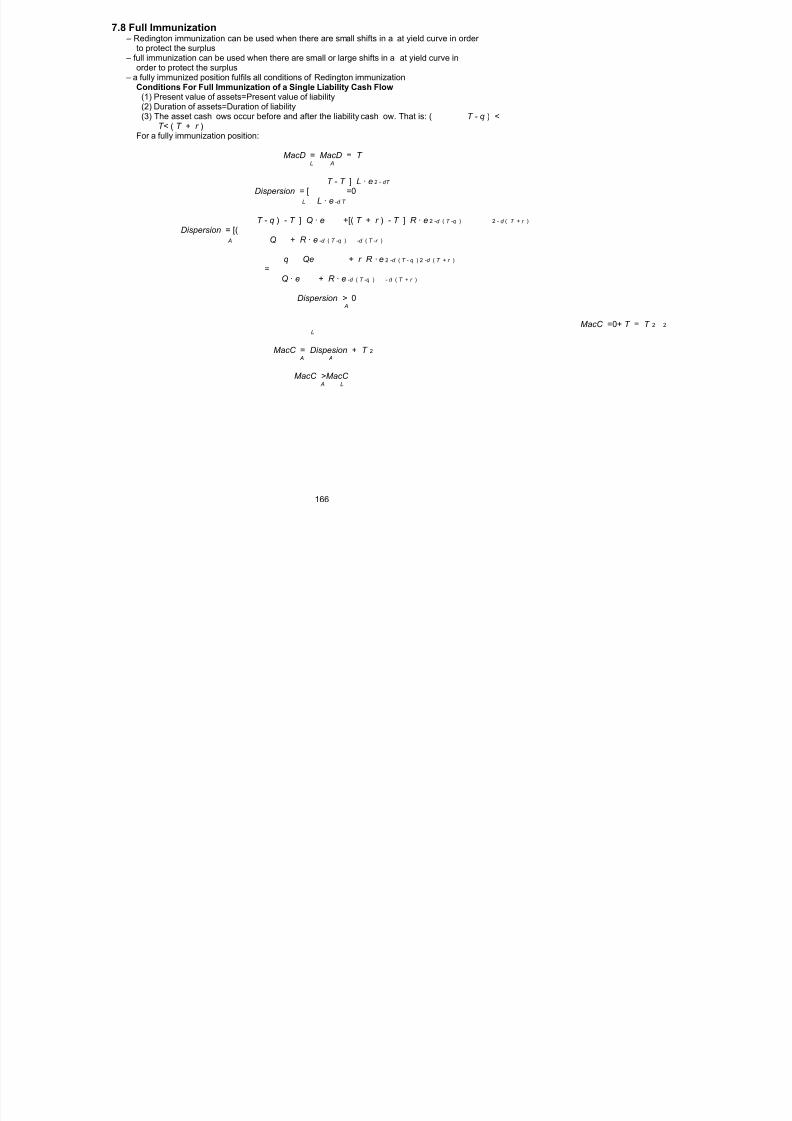
8/8/2019 3500145 Financial Math for Actuary and Businessman
http://slidepdf.com/reader/full/3500145-financial-math-for-actuary-and-businessman 168/181
7.8 Full Immunization – Redington immunization can be used when there are small shifts in a at yield curve in order
to protect the surplus – full immunization can be used when there are small or large shifts in a at yield curve in
order to protect the surplus – a fully immunized position fulfils all conditions of Redington immunization
Conditions For Full Immunization of a Single Liability Cash Flow(1) Present value of assets=Present value of liability(2) Duration of assets=Duration of liability(3) The asset cash ows occur before and after the liability cash ow. That is: ( T - q ) <
T< ( T + r )For a fully immunization position:
MacD = MacD = T L A
T - T ] L · e 2 - dT
Dispersion = [ =0L L · e -d T
T - q ) - T ] Q · e +[( T + r ) - T ] R · e 2 -d ( T -q ) 2 - d ( T + r )
Dispersion = [( A Q + R · e -d ( T -q ) -d ( T -r )
q Qe + r R · e 2 -d ( T - q ) 2 -d ( T + r )
=Q · e + R · e -d ( T -q ) - d ( T + r )
Dispersion > 0 A
MacC =0+ T = T 2 2L
MacC = Dispesion + T 2 A A
MacC >MacC A L
166
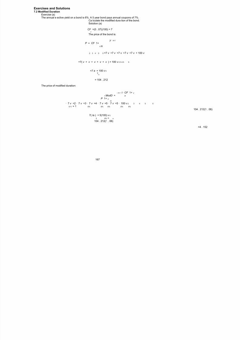
8/8/2019 3500145 Financial Math for Actuary and Businessman
http://slidepdf.com/reader/full/3500145-financial-math-for-actuary-and-businessman 169/181
Exercises and Solutions7.2 Modified Duration
Exercise (a)The annual e ective yield on a bond is 6%. A 5 year bond pays annual coupons of 7%.
Ca lculate the modified dura tion of the bond.Solution (a)
CF =(0 . 07)(100) = 7t
The price of the bond is:
y - m t
P = CF 1+t m
2 3 4 5 5 =7 v +7 v +7 v +7 v +7 v + 100 v
=7( v + v + v + v + v ) + 100 v 2 3 4 5 5
=7 a + 100 v 55
6%
= 104 . 212
The price of modified duration:
- m t t · CF 1+ y
t ModD = m
P 1+ y
m
· 7 v +2 · 7 v +3 · 7 v +4 · 7 v +5 · 7 v +5 · 100 v 2 3 4 5 5
6 % = 1 6% 6% 6% 6% 6%
104 . 212(1 . 06)
7( Ia ) + 5(100) v 5
5 6% = 6%
104 . 212(1 . 06)
=4 . 152
167

8/8/2019 3500145 Financial Math for Actuary and Businessman
http://slidepdf.com/reader/full/3500145-financial-math-for-actuary-and-businessman 170/181
Exercise (b)The current price of a bond is 116.73 and the current yield is 5%. The modified duration of the bond is 8.1 4. Use the modified duration to estimate the price of the bond if the yield
increases to 6.30%.Solution (b)
% P ˜ ( - y )( ModD )
˜ ( - 0 . 013)(8 . 14)
˜ ( -. 10582)
The bo nd price is:
116 . 73(1 - 0 . 10582) = 104 . 378
Exercise (c)A zero coupon bond matures in 10 years for 3,000. The bonds yield is 3% compoundedsemi-annua lly. Calculate the mo dified dura tion of the bond.Solution (c)
-m t y t · CF 1+t ModD = t m
P 1+ y
m
10(3 , 000)(1 . 015) - 20
3 , 000(1 . 015) (1 . 015) - 20
= 10 . 8521 . 015 =9
168

8/8/2019 3500145 Financial Math for Actuary and Businessman
http://slidepdf.com/reader/full/3500145-financial-math-for-actuary-and-businessman 171/181
Exercise (d)A two year bond has 6% annual coupons paid semi-annually. The bond’s yield is 8% semi-annually. Calculate the modified duration of the bond.
Solution (d)
- m t t · CF 1+ y
t ModD = m
P 1+ y
m
The semi-annual coupons are 0 . 03(100) = 3The semi-annual yield is =0 . 04 0 . 08
2
y -m t
Price = CF 1+t m
=3 v +3 v +3 v +3 v + 100 v 2 3 4 4
=3 a + 100 v 44
4%
P =96 . 3701
3(0 . 5 ) 3(1) 3(1 . 5) 3(2) 100(2) + + +1 . 04 (1 . 04 ) (1 . 04) (1 . 04) ( 1 . 04) 2 3 4 4 ModD =
96 . 3701 · (1 . 04)
2(100) 1 . 5( Ia ) +4 (1 . 04) 4 = 4 %
(96 . 3701)(1 . 04)
. 34528+ 170 . 96= 13 . 8389
100 . 2249 =1
169

8/8/2019 3500145 Financial Math for Actuary and Businessman
http://slidepdf.com/reader/full/3500145-financial-math-for-actuary-and-businessman 172/181
7.3 Macaulay DurationExercise (a)
The current price of a bond is 200. The derivative with respect to the yield to maturity is-800. The yield to maturity is 7%. Calculate the Macaulay duration.Solution (a)
-P ( y ) - ( - 800)ModD =
P ( y ) = 200 =4
MacDModD =
1+ y
m
MacD4=
1 . 07
MacD =4 . 28
170

8/8/2019 3500145 Financial Math for Actuary and Businessman
http://slidepdf.com/reader/full/3500145-financial-math-for-actuary-and-businessman 173/181
Exercise (b)Calculate the Macaulay duration of a common stock that pays dividends at the end of eachyear into perpetuity. Assume that the dividend is constant, and that the e ective rate of
interest is 8%.Solution (b)
8
t · CF v t t
t = 1 MacD =8
t CF v t
t = 1
8
t t · v t = 1 =
8
v t
t = 1
Solving for the numerator:
8
tv = v +2 v +3 v +4 v + ... + 8v t 2 3 4 8
t = 1
i = 1+
i 2Solving for the denominator:
8
v = v + v + v + v + ...v t 2 3 4 8
t = 1
= 1i
8
t · v t
i . 08 1+ i
t = 1 = = = 1+ = 1 . 5 i 2
i 0 . 08 =13 8 1
v t i
t = 1
171

8/8/2019 3500145 Financial Math for Actuary and Businessman
http://slidepdf.com/reader/full/3500145-financial-math-for-actuary-and-businessman 174/181
Exercise (c)Ca lculate the Macaulay Duration of a common stock that pays dividends at the end o f eachyear into perpetuity. Assume that the dividend increases by 3% each year and the e ective
rate is 5%.Solution (c)
8
t · CF v t t
t = 1 MacD =8
t CF v t
t = 1
8
t t- 1 t · v (1 . 03)t = 1 MacD =
8
v (1 . 03) t ( t- 1 )
t = 1
Solving for the numerator:
N = v (1 . 03) + 2 v (1 . 03) + 3 v (1 . 03) + ... + nv (1 . 03) 2 3 2 n n - 1
2 3 2 4 3 n n - 1 (1 . 03 v ) N =(1 . 03) v +2 v (1 . 03) +3 v (1 . 03) + ... +( n - 1) v (1 . 03) + ...
2 3 2 n - 1 n N - N (1 . 03) v = v + v (1 . 03) + v (1 . 03) + ... +(1 . 03) v + ...
N (1 - (1 . 03) v )= v (1 + v (1 . 03) + v (1 . 03) + ... +(1 . 03) v 2 2 n n
8
1 - 1 . 03
1+ i N (1 - (1 . 03) v )= v 1 - 1 . 03
1+ i
1N (1 - (1 . 03) v )= v
1 - (1 . 03) v
1N (1 - (1 . 03) v )= 1
1+ i 1 - 1 . 031+ i
1
N (1 - (1 . 03) v )= = 1 1+ i
i -
0 . 03 1+ i - 1 . 031+ i
i N = 1+
( i - 0 . 03) 2
172

8/8/2019 3500145 Financial Math for Actuary and Businessman
http://slidepdf.com/reader/full/3500145-financial-math-for-actuary-and-businessman 175/181
Now solving for the denominator:
= v + v (1 . 03) + v (1 . 03) + ... + v (1 . 03) 2 3 2 n n - 1
= v (1 + v (1 . 03) + v (1 . 03) + ... + v (1 . 03) 2 2 n - 1 n - 1
8
- 1 . 03
1 1+ i = v 1 - 1 . 03
1+ i
v 1=
1+ i 1 - 1 . 031+ i
1
= = 1 1+ i
i - . 03 i -. 031+ i
1+ i i . 05 . 05( i -. 03) 2 MacD = = 1+ . 5
i - . 03 = 1 0 . 05 - 0 . 03 = 1 0 . 02 =52 1i -. 03
Exercise (d)The duration of a bond at interest rate i is defined as:
t · CF v t
t t = 1
CF v t t = 1
t = 1
where CF represents the net cash ow from the coupons and the maturity value of the bondt
at time t . You are given a 1,000 par value 20-year bond with 4% annual coupons and amaturity value of 1,000. Calculate the duration of this bond at 5% interest.Solution (d)
Duration:
¨ a - 20 v 2 0
20 40 + 20(1 , 000) v 5 % 2 05%
Ia ) + 20(1 , 000) v 2 0 i 5%
20 5% = 40( =5%
40 a +1 , 000 v 40 a +1 , 000 v 20 2020 5% 20 5%
5 % 5%
11 , 975 . 81. 678
875 . 38 =13
173

8/8/2019 3500145 Financial Math for Actuary and Businessman
http://slidepdf.com/reader/full/3500145-financial-math-for-actuary-and-businessman 176/181
7.4 E ective DurationExercise (a)
a 10-year bond yielding 8% has a price of 112.76. If the bond yield falls to 7.75% then theprice of the bond will increase to 115.32. If the bond’s yield increases to 8.25% then the priceof the bond will fall to 110.25. Calculate the e ective duration of the bond.
Solution (a)
P - P - + EffD =
P (2 y )0
. 32 - 110 . 25 . 07= 115 . 9926
112 . 76(2)(0 . 0025) = 5 0 . 5638 =8
Exercise (b)A six year bond with coupons of 5% pays coupons semi-annually. The e ective yield is 4%.
It’s current price is 98.71. If the bond increases by 10 basis points then it’s price will fall to97.84. If the bond’s yield falls 10 basis points, then it’s price rises to 99.13. Caculate the
bond’s e ective duration.Solution (b)
P - P - + EffD =
P (2 y )0
. 13 - 97 . 84 . 29= 99 . 5346
(98 . 71)(2)(0 . 001) = 1 . 19742 =6
174

8/8/2019 3500145 Financial Math for Actuary and Businessman
http://slidepdf.com/reader/full/3500145-financial-math-for-actuary-and-businessman 177/181
7.5 ConvexityExercise (a)
The e ective duration is 5.4. The e ective convexity is calculated by a 2 0 year bond thathas an e ective yield of 7% and a price of 103.10. If the bond’s yield falls to 6.5% then theprice increases to 103.51. If the bond’s yield falls to 7.5% then the price decreases to 102.94.
Calculate the estimated new price of the bond if it increases by 75 basis points.Solution (a)
P + P - 2 P + - 0 EffC =
P ( y ) 20
. 51+ 102 . 94 - (2)(1 . 03 . 10)= 103
(103 . 10)( . 005) 2
. 25= 0 . 9932
. 0025775 =96
y ) 2
% P ˜- ( y )( Duration )+( Convexity )2 (
. 0075) 2
= - ( . 0075)(5 . 4) + ( . 9932)2 (96
= - 0 . 0378
175

8/8/2019 3500145 Financial Math for Actuary and Businessman
http://slidepdf.com/reader/full/3500145-financial-math-for-actuary-and-businessman 178/181
7.6 Duration, Convexity, and Prices: Putting it all Together Exercise (a)
Leah purchases three bonds to form a portfolio as follows:Bond A has semi-annual coupons at 5%, a duration of 20.57 years and was purchased for 880.
Bond B is an 11-year bond with a duration of 11.75 years and was purchased for 1,124.Bond C has a duration of 17.31 years and was purchased for 1,000.Ca lculate the duration of the portfolio at the time of purchase.Solution (a)The duration of the portfolio is:
P P P 1 2 n = D + D + ... + D
1 2 n MV MV MV po r t po r t po r t
MV = P + P + ...P po r t 1 2 n
MV = 880 + 1 , 124 + 1 , 000 = 3 , 004 po rt
. 57) , 124)(11 . 75) , 000)(17 . 31) , 8618 . 6Duration = (880)(20 . 18
po r t 3 , 004 + (1 3 , 004 + (1 3 , 004 = 4 3 , 004 =16
176

8/8/2019 3500145 Financial Math for Actuary and Businessman
http://slidepdf.com/reader/full/3500145-financial-math-for-actuary-and-businessman 179/181
8 The Term Structure of Interest RatesOverview
– this chapter will show how to:1. calculate a spot rate2. calculate a forward rate
8.1 Yield-to-Maturity – an interest rate is called a yield rate or an internal rate of return (IRR) as it indicates the
rate of return that the investor can expect to earn on their investment.finding price using a yield rate:
CF t P =
(1 + y ) t
t> 0
where P is price, t is time, CF is the cash ow and y is the yield ratet
Yield Curves – usually long-term market interest rates are higher than short-term market interest rates – yield curves are usually upsloping, although they can be at, downsloping, a peak or a valley – when the yield is constructed by government securities, it is called an on-the-run yield curve – when each bond’s coupon rate is assumed to equal a bond’s yield rate, it is called aparyield
curve
8.2 Spot Rates – are the annual interest rates that make up the yield curve. –let s represent the spot rate for period t .
t
–let P represent the net present value of a series of future payments (positive or negative)discounted using spot rates:
n
P = (1 + s ) · CF - t t t
t = 0
– The present value of annuities can also be found using spot rates:
a = 1 + 1 + ... + 1n 1+ s (1 + s ) (1 + s ) 2 n
1 2 n
¨ a =1+ 1 + 1 + ... + 1n 1+ s (1 + s ) (1 + s ) 2 n - 1
1 2 n - 1
177

8/8/2019 3500145 Financial Math for Actuary and Businessman
http://slidepdf.com/reader/full/3500145-financial-math-for-actuary-and-businessman 180/181
Bootstrapping – determining future spot rates using the price of a coupon bond – is used assuming arbitrage is impossible – arbitrage is risk-free profit
Price using yield=Price using spot rates
CF CF t t =
(1 + y ) (1 + s ) t t
t
Forward Rates – are considered to be future reinvestment rates.
the price of a security is calculated as follows:
CF t P =
(1 + f )(1 + f ) ··· (1 + f )0 1 t- 1
t> 0where f is the annual e ective forward rate from time t to t +1
t
– similar to the bo otstrapping concept, forward rates ca n be calculated using the yield curvePrice of yield curve=Price using forward rates
Relationships between Forward Rates and Spot Rates
(1 + s ) =(1+ f )(1 + f ) ··· (1 + f ) t
t 0 1 t- 1
s = (1 + f )(1 + f ) ··· (1 + f ) - 1t
t 0 1 t - 1
s ) t
t f = (1 + - 1t- 1 (1 + s ) t- 1
t- 1
Example:
A firm wishes to borrow money repayable in two years, where the one-year and two-year spotrates are 8% and 7%, respectively.
The estimated one-year deferred one-year spot rate is called the forward rate, f ,andiscalculated by equating the two interest ra tes such that
(1 . 08) =(1 . 07)(1 + f ) f =9 . 01% 2
If the bo rrower thinks that the spot rate for the 2 year will be greater(less) than the forward nd
rate, then they will select (reject) the 2-year borrowing rate.
178

8/8/2019 3500145 Financial Math for Actuary and Businessman
http://slidepdf.com/reader/full/3500145-financial-math-for-actuary-and-businessman 181/181
Related Documents