34th Annual Progress Report June 2013 Chapter 1 ...baydeltaoffice.water.ca.gov/modeling/deltamodeling/AR2013/Method... · 34th Annual Progress Report June 2013 Chapter 1 Temperature

Methodology for Flow and Salinity Estimates in the Sacramento-San Joaquin Delta and Suisun Marsh

34th Annual Progress Report June 2013

Chapter 1 Temperature Model Development for CalSim Authors: En-Ching Hsu and Prabhjot Sandhu,

Delta Modeling Section, Bay-Delta Office, California Department of Water Resources

Methodology for Flow and Salinity Estimates 34th Annual Progress Report

Page 1-ii SRWQM Temperature Model


Page 1-iii SRWQM Temperature Model

Contents 11 Temperature Model Development for CalSim ...................................................................................... 1-1

1.1 ABSTRACT .................................................................................................................................... 1-1

1.2 BACKGROUND .............................................................................................................................. 1-1

1.2.1 Assumptions ........................................................................................................................ 1-1

1.2.2 SRWQM ANN Training Framework and Linkage to CalSim ........................................... 1-3

1.2.3 Problem Setup .................................................................................................................... 1-4

1.3 ANN TRAINING ............................................................................................................................ 1-5

1.3.1 Comparison of ANN Network Parameter Setup ................................................................ 1-5

1.3.2 Selection of Input Variables ............................................................................................... 1-6

1.3.3 Selection of Input Memory ................................................................................................. 1-9

1.4 INTEGRATION SRWQM ANN TO CALLITE............................................................................... 1-11

1.4.1 Storage of SRWQM ANN Training Results ..................................................................... 1-11

1.4.2 Linearization of SRWQM ANN Results ........................................................................... 1-11

1.4.3 Temperature Estimates from CalLite .............................................................................. 1-12

1.5 SENSITIVITY ANALYSIS FOR SRWQM ANN TRAINING ........................................................... 1-19

1.6 DOWNSTREAM ANN TRAINING FOR BALLS FERRY.................................................................. 1-22

1.6.1 Downstream Water Temperature .................................................................................... 1-22

1.6.2 Downstream ANN Training for Balls Ferry .................................................................... 1-23

1.7 SUMMARY................................................................................................................................... 1-24

1.8 FUTURE DIRECTIONS .................................................................................................................. 1-25

1.9 ACKNOWLEDGEMENTS .............................................................................................................. 1-25

1.10 REFERENCES ............................................................................................................................... 1-25

Figures Figure 1-1 CalSim treatment of Shasta Reservoir .................................................................................................. 1-2

Figure 1-2 Schematic of layer definition in Shasta Reservoir ................................................................................ 1-2

Figure 1-3 SRWQM ANN training framework and linkage to CalSim ............................................................... 1-4

Figure 1-4 SRWQM versus ANN ........................................................................................................................... 1-5

Figure 1-5 Comparison between with and without air temperature and solar radiation ...................................... 1-7

Figure 1-6 Comparison between with and without inflow .................................................................................... 1-8

Figure 1-7 Comparison between with and without outflow from each layer ........................................................ 1-8

Figure 1-8 Comparison between different length of input memory ................................................................... 1-10


Page 1-iv SRWQM Temperature Model

Figure 1-9 Comparison between different length of input memory ................................................................... 1-10

Figure 1-10 SRWQM ANN CalSim integration and its time-step conversion .................................................. 1-11

Figure 1-11 Linearization for ANN results .......................................................................................................... 1-12

Figure 1-12 Comparison of release water temperature below Shasta for a baseline planning study ................ 1-14

Figure 1-13 Scatter plots by water year type for water temperature from SRWQM and CalLite .................... 1-16

Figure 1-14 Scatter plots by month for water temperature from SRWQM and CalLite ................................... 1-17

Figure 1-15 Comparison of release water temperatures below Shasta for an ELT climate change study ........ 1-20

Figure 1-16 Comparison of release water temperatures below Shasta for a LLT climate change study .......... 1-21

Figure 1-17 Schematic of HEC-5Q Upper Sacramento River Model ................................................................ 1-22

Figure 1-18 Water temperature at locations downstream of Shasta Reservoir .................................................. 1-23

Figure 1-19 Water temperature at Balls Ferry ..................................................................................................... 1-24


Page 1-1 SRWQM Temperature Model

11 Temperature Model Development for CalSim

1.1 Abstract River water temperature is important for the conservation of fishery habitat. Changes of water delivery or construction around waterways may impact fish mortality by changing river water temperature. Water temperature is highly relevant to fish mortality and also indirectly influences habitat. Current temperature modeling takes flow output from CalSim1 and then estimates temperature at points of interest. However, when the downstream temperature requirement is violated, there is no way to adjust outflow or storage to lower the impact.

The purpose of this study is to integrate the Sacramento River Water Quality Model (SRWQM) into CalSim and make reasonable accurate estimates for released water temperature. Artificial Neural Network (ANN) technology is used to capture the behavior of SRWQM by training datasets. A simple system with inflow, storage and outflow is set up around Shasta Lake. The reservoir itself is divided into four layers (top, middle, penstock and lower) and layer temperature is estimated based on given inputs (air temperature, solar radiation, storage, and inflow). Temperature Control Devices (TCDs) were installed in Shasta Lake in 1997 and allow water released from different combination of layers to meet the target downstream river temperature. Through this integration, CalSim can adjust flow or storage to meet river temperature requirements.

1.2 Background The SRWQM was developed using the HEC-5Q model to simulate mean daily reservoir and river temperature (using 6-hour meteorology data) at Shasta, Trinity, Lewiston, Whiskeytown, Keswick and Black Butte Reservoir and Trinity River, Clear Creek and the upper Sacramento River from Shasta to Knights Landing and Stony Creek. SRWQM simulates flows with TCDs so the released flow is a mixture of water from top, middle, penstock or lower layers of reservoir. SRWQM takes CalSim outputs (flow and storage) as inputs. Temperature outputs from SRWQM are further used in fish mortality models, such as SALMOD2 and the Reclamation Temperature Model.3

1.2.1 Assumptions

1) In CalSim, a simple system is simulated around Lake Shasta (Figure 1-1).

2) The delineation of top, middle, penstock and lower layers for Shasta Reservoir is defined in Figure 1-2. The elevation and storage values are approximations from SRWQM.

3) SRWQM is a daily time-step model. To mimic SRWQM as close as possible, a daily time-step is used for ANN training.

4) Since CalSim uses a monthly time-step, it is necessary to convert from monthly to daily values to use ANN training results. Data from CalSim are reservoir inflow and storage. These are assumed

1 CalSim is the model used to simulate California State Water Project (SWP)/Central Valley Project (CVP) operations (California Dept. of Water Resources). 2 SALMOD is the model used to simulate the dynamics of freshwater salmonid population (U.S. Geologocal Survey). 3 U.S. Bureau of Reclamation Temperature Model simulates monthly mean vertical temperature profiles and release temperatures (U.S. Bureau of Reclamation).



constant for all daily data points. This avoids the possible violation of mass conservation from spline fitting.

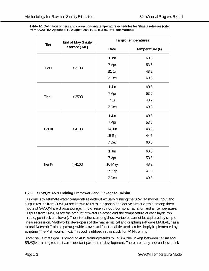
5) In SRWQM, Shasta TCDs operate by the rules defined in four Tier operations based on end-of-May Shasta storage (Table 1-1). Monthly target temperatures are calculated at each CalSim time-step so that CalSim can mimic the operation in SRWQM.

6) Water temperature downstream of Shasta Reservoir is assumed to be the mixture from the four layers as shown. Water leakages or seepages from reservoir are ignored because of its relatively small amount and having less impact of downstream water temperature.

Figure 1-1 CalSim treatment of Shasta Reservoir

Figure 1-2 Schematic of layer definition in Shasta Reservoir



Table 1-1 Definition of tiers and corresponding temperature schedules for Shasta releases (cited from OCAP BA Appendix H, August 2008 (U.S. Bureau of Reclamation))

Tier End of May Shasta Storage (TAF)

Target Temperatures

Date Temperature (F)

Tier I < 3100

1 Jan

7 Apr

31 Jul

7 Dec

60.8

53.6

48.2

60.8

Tier II < 3500

1 Jan

7 Apr

7 Jul

7 Dec

60.8

53.6

48.2

60.8

Tier III < 4100

1 Jan

7 Apr

14 Jun

15 Sep

7 Dec

60.8

53.6

48.2

44.6

60.8

Tier IV > 4100

1 Jan

7 Apr

10 May

15 Sep

7 Dec

60.8

53.6

48.2

41.0

60.8

1.2.2 SRWQM ANN Training Framework and Linkage to CalSim

Our goal is to estimate water temperature without actually running the SRWQM model. Input and output results from SRWQM are known to us so it is possible to derive a relationship among them. Inputs of SRWQM are Shasta storage, inflow, reservoir outflow, solar radiation and air temperature. Outputs from SRWQM are the amount of water released and the temperature at each layer (top, middle, penstock and lower). The interactions among those variables cannot be captured by simple linear regression. Mathworks, developers of the mathematical and graphing software MATLAB, has a Neural Network Training package which covers all functionalities and can be simply implemented by scripting (The Mathworks, Inc.). This tool is utilized in this study for ANN training.

Since the ultimate goal is providing ANN training results to CalSim, the linkage between CalSim and SRWQM training results is an important part of this development. There are many approaches to link



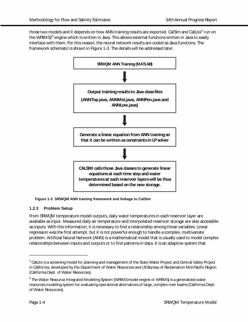
those two models and it depends on how ANN training results are exported. CalSim and CalLite4 run on the WRIMS25 engine which is written in Java. This allows external functions written in Java to easily interface with them. For this reason, the neural network results are coded as Java functions. The framework schematic is shown in Figure 1-3. The details will be addressed later.

Figure 1-3 SRWQM ANN training framework and linkage to CalSim

1.2.3 Problem Setup

From SRWQM temperature model outputs, daily water temperatures in each reservoir layer are available as input. Measured daily air temperature and interpolated reservoir storage are also accessible as inputs. With this information, it is necessary to find a relationship among those variables. Linear regression was the first attempt, but it is not powerful enough to handle a complex, multivariate problem. Artificial Neural Network (ANN) is a mathematical model that is usually used to model complex relationships between inputs and outputs or to find patterns in data. It is an adaptive system that

4 CalLite is a screening model for planning and management of the State Water Project and Central Valley Project in California, developed by the Department of Water Resources and US Bureau of Reclamation Mid-Pacific Region (California Dept. of Water Resources). 5 The Water Resource Integrated Modeling System (WRIMS model engine or WRIMS) is a generalized water resources modeling system for evaluating operational alternatives of large, complex river basins (California Dept. of Water Resources).

SRWQM ANN Training (MATLAB)

Output training results to Java class files

(ANNTop.java, ANNMid.java, ANNPen.java and ANNLow.java)

CALSIM calls those Java classes to generate linear equations at each time step and water

temperatures at each reservoir layers will be thus determined based on the new storage.

Generate a linear equation from ANN training so that it can be written as constraints in LP solver



changes its structure based on external or internal information that flows through the networks during the learning phase. For time series data analysis, it is important to consider past data that may carry their influence for current time-step, that is, the system may have memory.

The testing setup uses SRWQM temperature model results from a baseline planning study. The simulation period of SRWQM is from October 1, 1921 to September 30, 2003. Since the first few years initialize the simulation and are not considered valid model output, the ANN training period is from October 1, 1925 to September 30, 2003. Before the evaluation of input variables, some results from adjusting ANN training parameters are shown to have a good sense of how ANN behaves. Inputs use up to the previous four weeks air temperature and previous two weeks Shasta storage.

SRWQM is a physically-based model that accounts for mass, heat balance, and transfer. It requires meteorological data and hydrological data for each time-step to perform complex computation. Shasta Reservoir is a strongly stratified reservoir; temperature control devices (TCD) were installed in 1997 to withdraw water from different layers. This structure allows operators to access water at multiple elevations in order to maintain cool water releases without bypassing power generators. With the operation of TCDs, the water mixing inside reservoir becomes more complicated and hard to estimate. Mass balance may be straightforward but heat balance is difficult to calculate with simple models. We provide water release from each layer as input in the ANN so that the ANN can implicitly consider heat balance and mixing. Without understanding physical interaction, the ANN searches for the best relationship between input and outputs. Once the relationship is obtained, the output can be easily calculated from matrix multiplication. As Figure 1-4 shows, ANN is used to replace complex computation and the physical-based model, yielding results consistent with SRWQM. The release water temperature below Shasta (T) is calculated by Equation 1.

= + + + /( + + + ) Eq.1

Figure 1-4 SRWQM versus ANN

1.3 ANN Training 1.3.1 Comparison of ANN Network Parameter Setup

An ANN simulation has many different possible configurations, and it is not obvious beforehand which will yield the best results. Some tests have been carried out to observe the sensitivity of ANN parameter changes. The ANN parameters used for this study are:

SRWQM

Physically-based model: mass balance,

heat balance

Inputs:

Meteorological and hydrologic data

Outputs:

Water temperature at four layers and water mixed to meet target temperature

Inputs:

Meteorological and hydrologic data

ANN

Mathematical adaptive system (Black box)

Outputs:

Water temperature at four layers and water mixed to meet target temperature



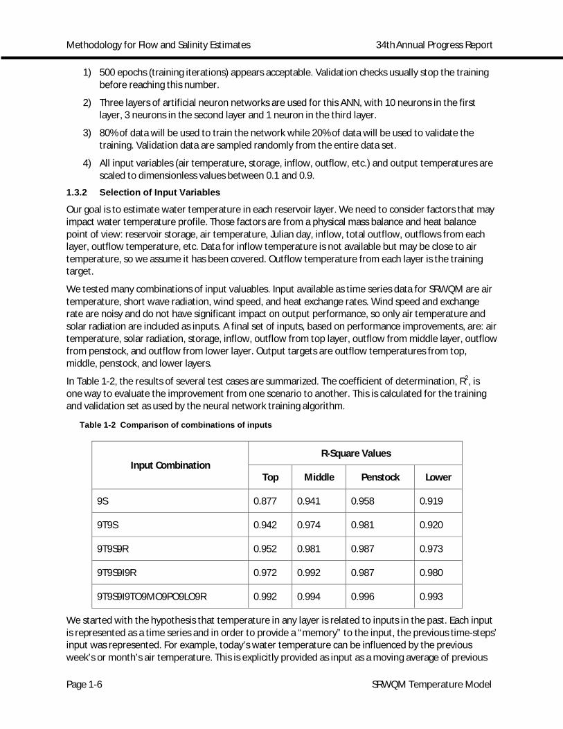
1) 500 epochs (training iterations) appears acceptable. Validation checks usually stop the training before reaching this number.

2) Three layers of artificial neuron networks are used for this ANN, with 10 neurons in the first layer, 3 neurons in the second layer and 1 neuron in the third layer.

3) 80% of data will be used to train the network while 20% of data will be used to validate the training. Validation data are sampled randomly from the entire data set.

4) All input variables (air temperature, storage, inflow, outflow, etc.) and output temperatures are scaled to dimensionless values between 0.1 and 0.9.

1.3.2 Selection of Input Variables

Our goal is to estimate water temperature in each reservoir layer. We need to consider factors that may impact water temperature profile. Those factors are from a physical mass balance and heat balance point of view: reservoir storage, air temperature, Julian day, inflow, total outflow, outflows from each layer, outflow temperature, etc. Data for inflow temperature is not available but may be close to air temperature, so we assume it has been covered. Outflow temperature from each layer is the training target.

We tested many combinations of input valuables. Input available as time series data for SRWQM are air temperature, short wave radiation, wind speed, and heat exchange rates. Wind speed and exchange rate are noisy and do not have significant impact on output performance, so only air temperature and solar radiation are included as inputs. A final set of inputs, based on performance improvements, are: air temperature, solar radiation, storage, inflow, outflow from top layer, outflow from middle layer, outflow from penstock, and outflow from lower layer. Output targets are outflow temperatures from top, middle, penstock, and lower layers.

In Table 1-2, the results of several test cases are summarized. The coefficient of determination, R2, is one way to evaluate the improvement from one scenario to another. This is calculated for the training and validation set as used by the neural network training algorithm.

Table 1-2 Comparison of combinations of inputs

Input Combination R-Square Values

Top Middle Penstock Lower

9S 0.877 0.941 0.958 0.919

9T9S 0.942 0.974 0.981 0.920

9T9S9R 0.952 0.981 0.987 0.973

9T9S9I9R 0.972 0.992 0.987 0.980

9T9S9I9TO9MO9PO9LO9R 0.992 0.994 0.996 0.993

We started with the hypothesis that temperature in any layer is related to inputs in the past. Each input is represented as a time series and in order to provide a “memory” to the input, the previous time-steps’ input was represented. For example, today’s water temperature can be influenced by the previous week’s or month’s air temperature. This is explicitly provided as input as a moving average of previous



time-steps. These are sampled as current time t, t -7days, t -21, t -35, t -49, t -63, t -77, t -91, t -105, t -119, etc. All values are 7-day moving averages.

Each input variable is abbreviated with simple notation. For example, 9T9S9I9TO9MO9PO9LO9R stands for 9 prior weekly (as defined above) air temperatures (T, Tt-7, Tt-21, …, Tt-105), 9 storages (S), 9 inflows (I), 9 outflows from the top layer (TO), the middle layer (MO), the penstock layer (PO), the lower layer (LO), and 9 solar radiations (R).

From Table 1-2, the results make sense: higher R2 values are seen with more inputs to the ANN. Besides looking at R2 values, we also investigated the results through time series plots in order to help us view the effects of the inputs in more detail.

1) With storage alone, the water temperature profile in each layer can be roughly captured with R2 > 0.88.

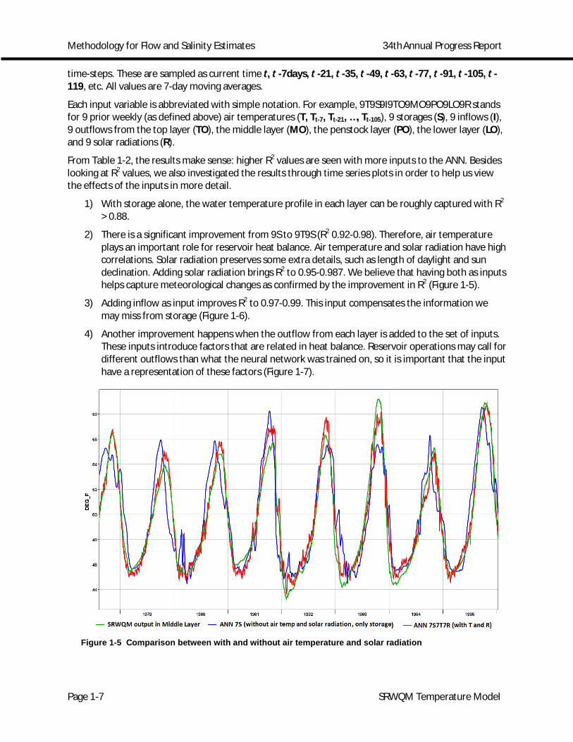
2) There is a significant improvement from 9S to 9T9S (R2 0.92-0.98). Therefore, air temperature plays an important role for reservoir heat balance. Air temperature and solar radiation have high correlations. Solar radiation preserves some extra details, such as length of daylight and sun declination. Adding solar radiation brings R2 to 0.95-0.987. We believe that having both as inputs helps capture meteorological changes as confirmed by the improvement in R2 (Figure 1-5).

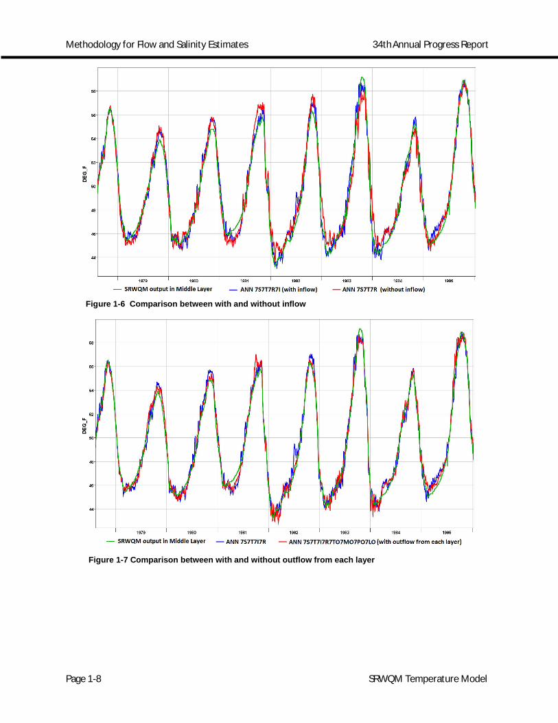
3) Adding inflow as input improves R2 to 0.97-0.99. This input compensates the information we may miss from storage (Figure 1-6).

4) Another improvement happens when the outflow from each layer is added to the set of inputs. These inputs introduce factors that are related in heat balance. Reservoir operations may call for different outflows than what the neural network was trained on, so it is important that the input have a representation of these factors (Figure 1-7).

Figure 1-5 Comparison between with and without air temperature and solar radiation



Figure 1-6 Comparison between with and without inflow

Figure 1-7 Comparison between with and without outflow from each layer



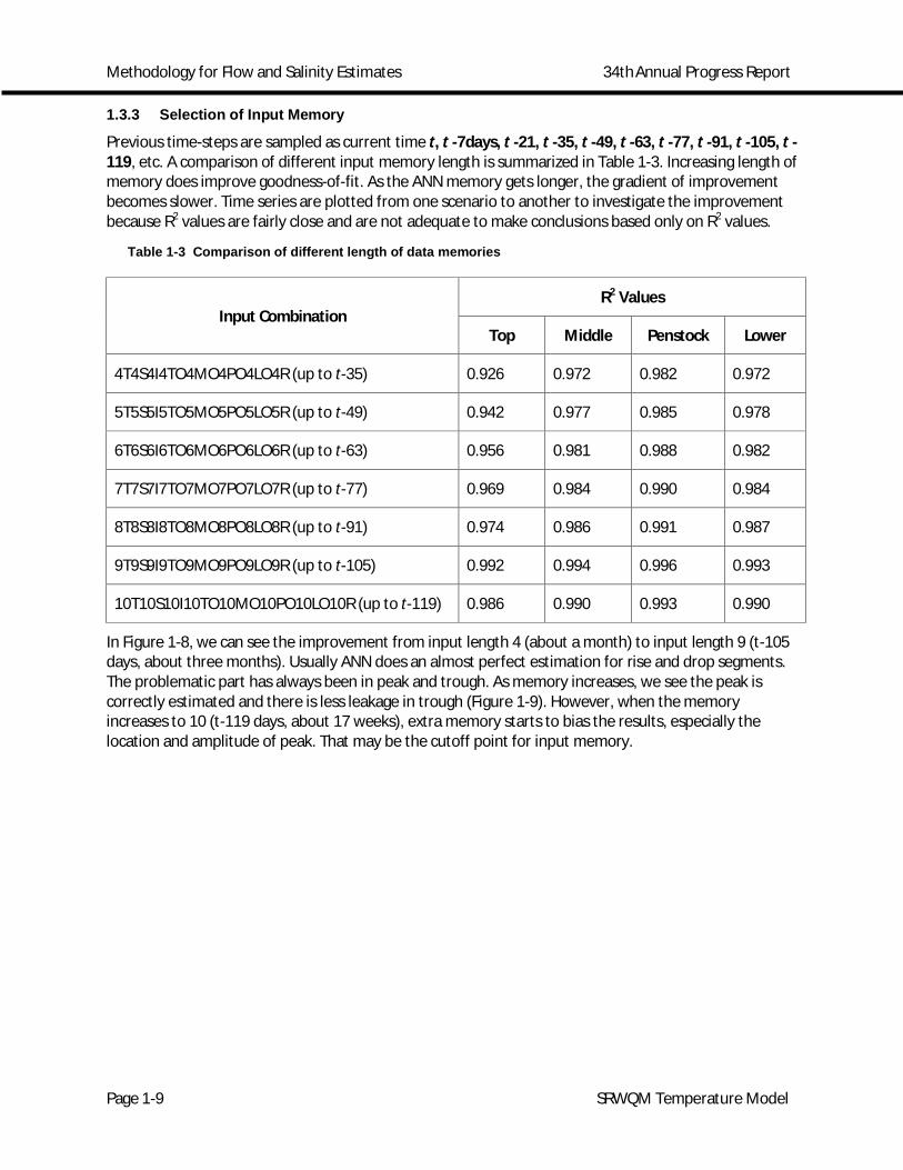
1.3.3 Selection of Input Memory

Previous time-steps are sampled as current time t, t -7days, t -21, t -35, t -49, t -63, t -77, t -91, t -105, t -119, etc. A comparison of different input memory length is summarized in Table 1-3. Increasing length of memory does improve goodness-of-fit. As the ANN memory gets longer, the gradient of improvement becomes slower. Time series are plotted from one scenario to another to investigate the improvement because R2 values are fairly close and are not adequate to make conclusions based only on R2 values.

Table 1-3 Comparison of different length of data memories

Input Combination R2 Values

Top Middle Penstock Lower

4T4S4I4TO4MO4PO4LO4R (up to t-35) 0.926 0.972 0.982 0.972







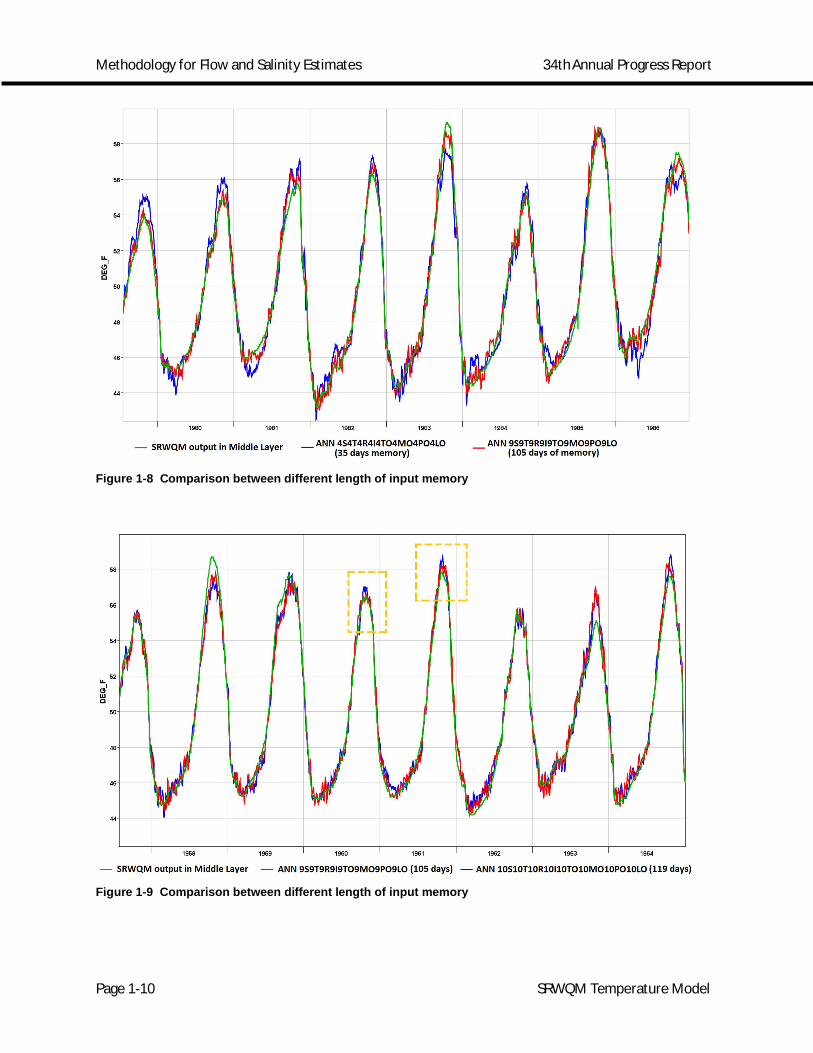
In Figure 1-8, we can see the improvement from input length 4 (about a month) to input length 9 (t-105 days, about three months). Usually ANN does an almost perfect estimation for rise and drop segments. The problematic part has always been in peak and trough. As memory increases, we see the peak is correctly estimated and there is less leakage in trough (Figure 1-9). However, when the memory increases to 10 (t-119 days, about 17 weeks), extra memory starts to bias the results, especially the location and amplitude of peak. That may be the cutoff point for input memory.



Figure 1-8 Comparison between different length of input memory

Figure 1-9 Comparison between different length of input memory



1.4 Integration SRWQM ANN to CalLite 1.4.1 Storage of SRWQM ANN Training Results

CalSim and CalLite use the WRIMS2 Engine, which is written in Java, so coding external functions in Java makes direct connections without translation through another computer language. ANN training results for each layer is stored separately in four Java class files.

SRWQM is a daily time-step model, so in order to preserve the model behavior, ANN training is performed for original daily inputs and outputs. However, CalSim is a monthly operation model, so data conversion is necessary. The process is shown in Figure 1-10. Monthly inputs are Shasta storage and inflow. Metrological data, such as solar radiation and air temperature, are read in as daily data since it is independent of CalSim operation.

Figure 1-10 SRWQM ANN CalSim integration and its time-step conversion

1.4.2 Linearization of SRWQM ANN Results

There is an additional effort for this integration, the conversion between ANN nonlinearity and LP linear constraints. CalSim and CalLite are programmed in WRESL code which is a simulation language for flexible operational criteria and uses a linear programming (LP) solver to allocate water efficiently. In order to do so, all the constraints must be given in the form of linear equations. If not, the compiler will reject the nonlinearity and not solve the problem. We follow the approach that has been adopted in DSM2 EC ANN training(Seneviratne & Wu, 2007). A contour line of a given constant EC is calculated from EC ANN training which is a function of Sacramento flow and export. Once the contour is calculated, a box is applied (Figure 1-11a) to define the intersecting points so that the contour can be approximated by a straight line. This will provide a linear equation which is recognizable in the LP solver.

From previous SRWQM ANN training evaluations, inputs used to estimate water temperature are air temperature (T), solar radiation (R), inflow (known), Shasta storage (S) and outflows (TO, MO, PO, LO) from each layer (unknown). In the training evaluation, there is about 1% improvement from with-outflow to without-outflow. However, when integrating with CalSim, if outflows from each layer are considered for linearization, there will be five unknowns and it increases the complexity for linearization. The variations of outflows from each layer are high and lots of assumptions need to be made in order to linearize the problem. Those assumptions and trial-and-error guesses introduce unsteady outputs and cumbersome iterations. The error and bias can easily exceed 1% by a significant margin. Therefore, outflows are dropped from linearization to simplify and stabilize the problem.

SRWQM was trained in daily time step

CALSIM operates in monthly time step

Convert monthly input to daily input (assume constant for all data within a month)

Create input memory from daily data and call Java classes to estimate the slope and intercept for linear equations

Return the linear equations to CALSIM as constraints for the current time step



In SRWQM ANN training, air temperature, solar radiation and inflow are known. The only decision variable is Shasta storage. Therefore, simple linear fitting between water temperature and storage can approximate the relationship (Figure 1-11b). To make a reasonable fitting, the range of sampling points is selected based on the previous time-step Shasta storage and current inflow. This will ensure those points covering the possible range of storage for the current time-step. This line is calculated at each time-step, so it provides a real time relationship between storage and water temperature based on air temperature, solar radiation and inflow happening in that month.

(a)

(b)

Figure 1-11 Linearization for ANN results

1.4.3 Temperature Estimates from CalLite

Water temperatures at four layers (top, middle, penstock, and lower) are estimated by ANN training results while Shasta storage is determined by CalLite optimization. Shasta Lake has the TCD so it can adjust water released from each layer to meet downstream water temperature requirement.

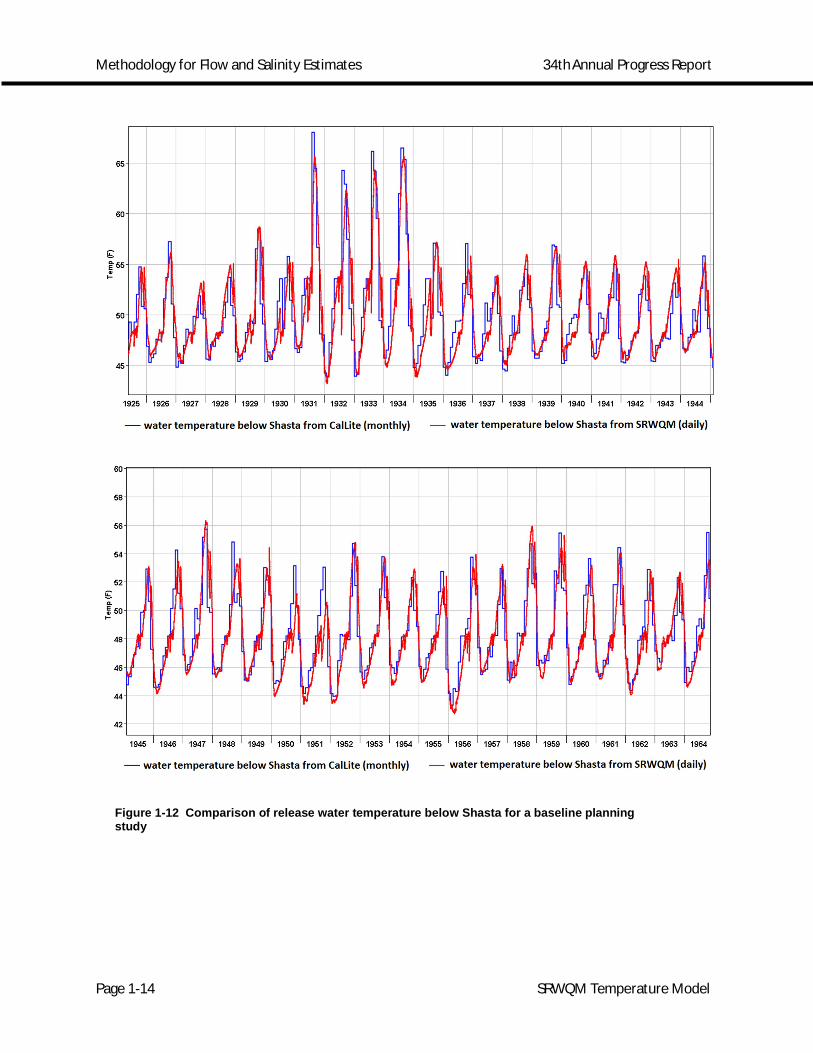
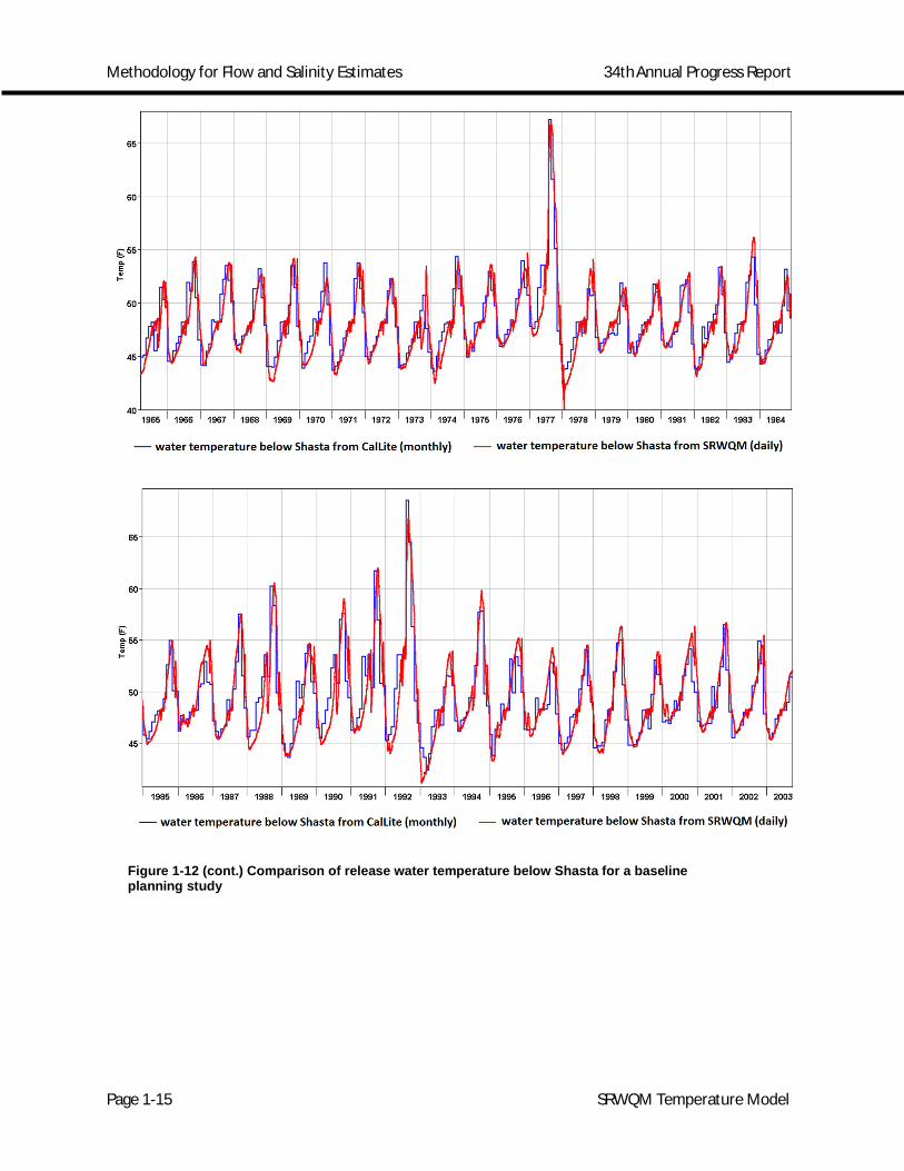
In this study, we used a baseline planning study for ANN training. The simulation period is from 1921 to 2003. To investigate the performance of CalLite SRWQM-ANN, the most straightforward approach is comparing time series plots. The 82-year runs are presented in Figure 1-12. We divided the entire time series into four plots for more detail. The red line is the Shasta release water temperature from SRWQM daily model and the blue line is the temperature from a simple CalLite setup which is a monthly operation model. Traveling through time, CalLite captures the overall pattern fairly well, especially in rising segments, descending segments and troughs. There are greater differences in peaks. However, the differences rarely exceed 3oF and in most years it matches surprisingly well in spite of the complexities during the dry seasons.

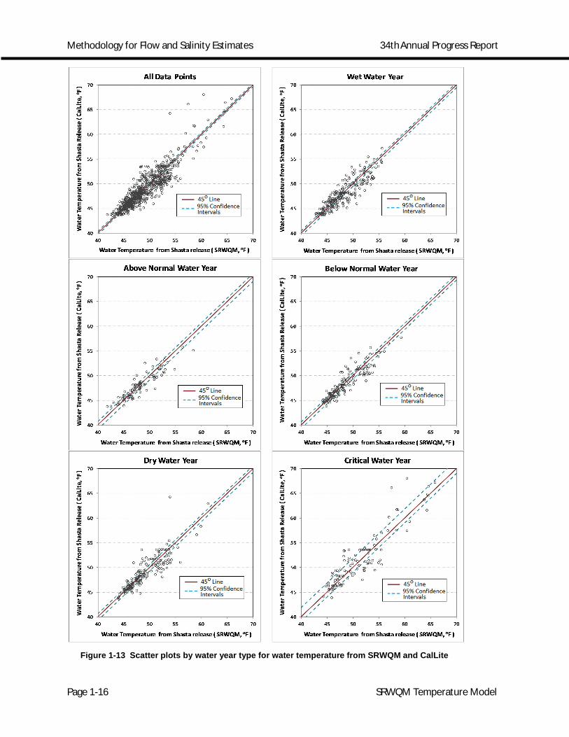
Scatter plots help us interpret the results in more detail, such as analyzing results based on water year types or months. In Figure 1-13, there are scatter plots for all points and five water year types (wet, above normal, below normal, dry and critical). The X axis is the water temperature from SRWQM while the Y axis is the water temperature from CalLite. A 45 degree line is shown to help visually interpret the goodness-of-fit. Upper and lower 95% confidence intervals are also shown to help us get a good sense of range of estimations.

By looking at water year type (Figure 1-13), the results scatter around the 45 degree line with 95% confidence limit within 1oF. The only exception is critical water years in which the confidence interval increases to 2oF and CalLite is more likely to overestimate the water temperature. Overall, release water temperature in wet years ranges from 43 oF to 56 oF, above normal year from 42 oF to 60 oF, below normal year from 44 oF to 60 oF, dry year from 44 oF to 62 oF and critical year from 44 oF to 67 oF.



By evaluating the results for individual months, we observe that CalLite is more likely to slightly overestimate the temperature from February to October and underestimate temperature from November to January. Overall, release water temperature in Jan ranges from 44 oF to 50 oF, Feb from 43

oF to 48 oF, Mar from 43 oF to 48 oF, Apr from 44 oF to 51 oF, May from 45 oF to 54 oF, Jun from 46 oF to 54

oF, Jul from 47 oF to 60 oF, Aug from 48 oF to 65 oF, Sep from 47 oF to 65 oF, Oct from 47 oF to 62 oF, Nov from 50 oF to 57 oF and Dec from 47 oF to 55 oF. The high variation (wide confidence intervals) happens in the months of August and September.



Figure 1-12 Comparison of release water temperature below Shasta for a baseline planning study



Figure 1-12 (cont.) Comparison of release water temperature below Shasta for a baseline planning study



Figure 1-13 Scatter plots by water year type for water temperature from SRWQM and CalLite



Figure 1-14 Scatter plots by month for water temperature from SRWQM and CalLite



Figure 1-14 (cont.) Scatter plots by month for water temperature from SRWQM and CalLite



1.5 Sensitivity Analysis for SRWQM ANN Training The sensitivity analysis for this project is studying the effect of changes in input parameter values on output temperature values. In this study we are delivering a proof-of-concept case and we are inviting feedback from various user and expert groups before we invest the substantial effort required to conduct such an analysis.

We would typically study such sensitivity by parameter perturbation. For example we would independently perturb air temperature, inflow and outflow by 10% and run the model to see temperature responds to those changes of each parameter.

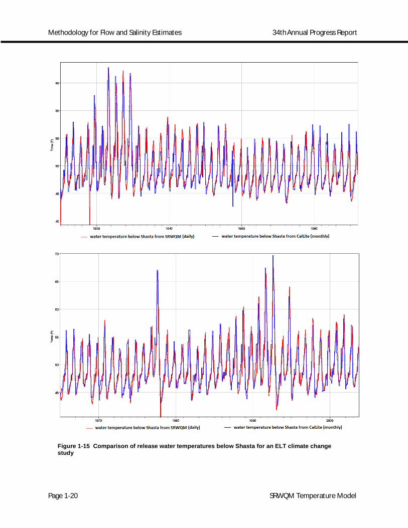
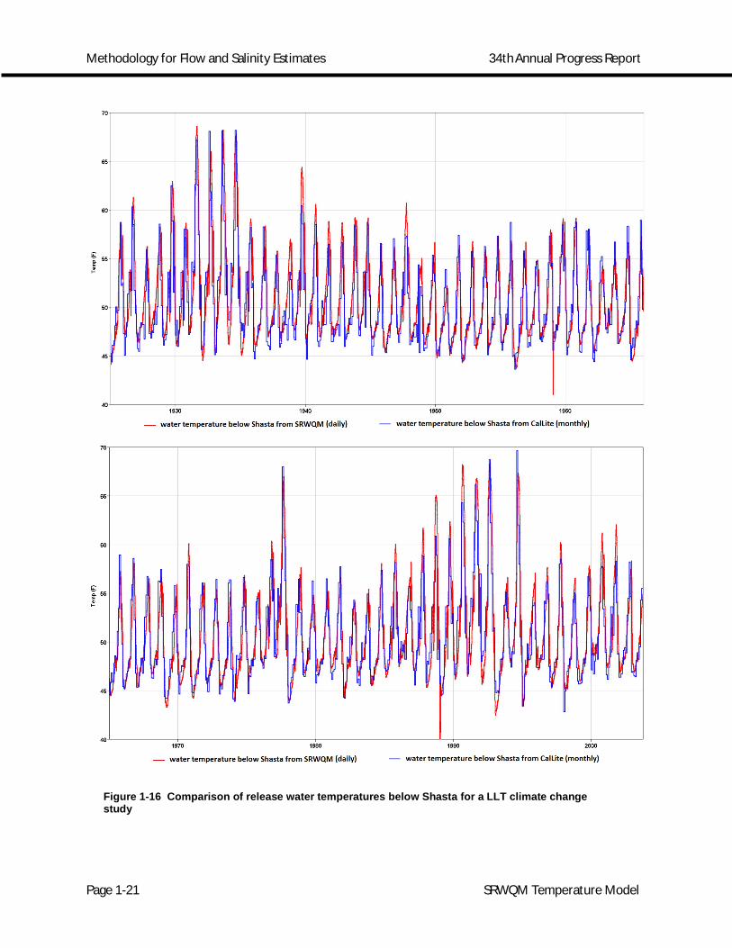
We did a preliminary study involving climate change scenarios, named as Early Long Term (ELT) and Late Long Term (LLT). The aim was to see how an ANN trained on this data responds to different input data sets, such as higher or lower outflow and different meteorological data. We were looking for poor estimation or bias which would imply that the training sets are not sufficient to represent model behavior.

The comparison of water temperature below Shasta from CalLite and SRWQM for ELT and LLT are shown in Figure 1-15 and Figure 1-16, respectively. Note that outputs from CalLite are monthly while outputs from SRWQM are daily. Overall, we did not see any major changes in those plots and this implies that the training set is sufficient in capturing these relationships. However, training with wider range data is recommended to precisely quantify the relationship between inputs and outputs.



Figure 1-15 Comparison of release water temperatures below Shasta for an ELT climate change study



Figure 1-16 Comparison of release water temperatures below Shasta for a LLT climate change study



1.6 Downstream ANN Training for Balls Ferry The previous ANN training was used to define the water temperature of each layer so that CalSim can decide how to mix water to achieve target temperatures below Shasta. However, biological points of interest often are further downstream. As water travels, its temperature is affected by air temperature, solar radiation, Shasta released water quantity, and tributary water temperatures. The goal is to define the water temperature releases from Shasta in order to meet the temperature requirements at particular downstream locations.

1.6.1 Downstream Water Temperature

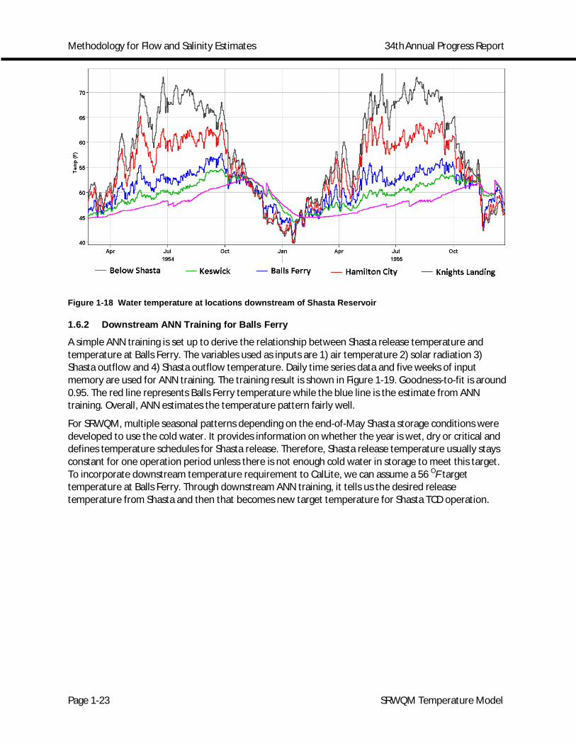
The output locations in SRWQM are shown in Figure 1-17. Through the TCD, we are able to decide how to release water to meet target release water temperatures. This may be limited to immediately downstream of Shasta Dam. As water travels further downstream, water temperature is more dominated by air temperature. Taking Figure 1-18 for instance, water temperature below Keswick and Balls Ferry still follow the pattern of water below Shasta Reservoir. However, Shasta water releases do not have much influence on river temperatures near Hamilton City and Knights Landing. Right now we follow the temperature control target in SRWQM which is based on end-of-May Shasta storage. We may need to know locations and temperature requirement so that we can define violation criterion in SRWQM and later in the CalSim operation.

Figure 1-17 Schematic of HEC-5Q Upper Sacramento River Model



Figure 1-18 Water temperature at locations downstream of Shasta Reservoir

1.6.2 Downstream ANN Training for Balls Ferry

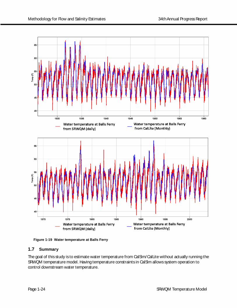
A simple ANN training is set up to derive the relationship between Shasta release temperature and temperature at Balls Ferry. The variables used as inputs are 1) air temperature 2) solar radiation 3) Shasta outflow and 4) Shasta outflow temperature. Daily time series data and five weeks of input memory are used for ANN training. The training result is shown in Figure 1-19. Goodness-to-fit is around 0.95. The red line represents Balls Ferry temperature while the blue line is the estimate from ANN training. Overall, ANN estimates the temperature pattern fairly well.

For SRWQM, multiple seasonal patterns depending on the end-of-May Shasta storage conditions were developed to use the cold water. It provides information on whether the year is wet, dry or critical and defines temperature schedules for Shasta release. Therefore, Shasta release temperature usually stays constant for one operation period unless there is not enough cold water in storage to meet this target. To incorporate downstream temperature requirement to CalLite, we can assume a 56 OF target temperature at Balls Ferry. Through downstream ANN training, it tells us the desired release temperature from Shasta and then that becomes new target temperature for Shasta TCD operation.



Figure 1-19 Water temperature at Balls Ferry

1.7 Summary The goal of this study is to estimate water temperature from CalSim/CalLite without actually running the SRWQM temperature model. Having temperature constraints in CalSim allows system operation to control downstream water temperature.



The Sacramento River Water Quality Model (SRWQM) is the temperature model selected for ANN training. It was developed to simulate mean daily reservoir and river temperatures. A single reservoir system around Shasta Lake is set up for testing. The components are inflow, outflow (downstream water demand plus flood control spills) and storage. It is assumed that downstream demand is the same as outflow from Shasta in a baseline study. Shasta Lake is vertically divided into four layers and water temperatures at each layer are available from SRWQM. Artificial Neural Networks (ANNs) can be trained to simulate water temperatures in each layer based on given inputs: air temperature, solar radiation, Shasta storage and inflow. The effect of each input on temperature output can be seen over a period of time. This memory effect is represented by explicitly specifying up to 3 months of past input values.

With given inflow and total outflow, the TCD releases water from different layers to meet downstream temperature requirement. For now, temperature does not control total outflow unless some further constraints are given or CalSim allows back optimizations.

Integration of SRWQM ANN into CalLite WRESL code was done by generating Java classes based on training data. This allows a direct interface with the WRIMS Java Engine.

The relationship from Shasta to downstream locations, such as Balls Ferry, is also derived, based on air temperature, solar radiation, Shasta released flow, and temperature. Further downstream, water temperature is dominated by air temperature.

ANN training is validated with high correlation (R2 approaching 1) ranging from 0.97 to 0.99. A baseline planning study is used for training and temperatures are evaluated by comparing the results from SRWQM and CalLite. CalLite captures SRWQM quite well.

Detail sensitivity analysis will be done later. For now, other scenarios with climate changes (ELT and LLT) have been tested and ANN performs well.

1.8 Future Directions 1. This study has tested a simple single model around Shasta. To incorporate this additional

temperature feature into CalSim and CalLite, ANN training results and codes will be delivered to the CalSim/CalLite team so that they can evaluate this new feature.

2. We assumed outflow is equal to downstream demand, and that water temperatures are determined based on the outflow is a given. With a fixed outflow, TCD releases water from different layers to meet target temperature. If the outflow violates a temperature constraint, a penalty is added to the optimization but this does not change outflow to alter the result. Therefore, temperature has no control for total release outflow as well as storage. Right now, we can only estimate release temperature based on given flows. The decision of outflow and storage changes needs to be evaluated by looking at the entire system.

3. Sensitivity analyses can be done either through ANN training or CalLite problem solving. This will be management’s call for timelines and necessary efforts.

1.9 Acknowledgements Kuo-Cheng Kao and Hao Xie of DWR provided help in CalLite integration.

1.10 References California Dept. of Water Resources. (n.d.). CalLite: Central Valley Water Management Screening Model. Retrieved April 2013, from http://baydeltaoffice.water.ca.gov/modeling/hydrology/CalLite/index.cfm



California Dept. of Water Resources. (n.d.). WRIMS Model Engine and CalSim Model. Retrieved April 2013, from Bay-Delta Office, Central Valley Water Resources System Modeling: http://baydeltaoffice.water.ca.gov/modeling/hydrology/CalSim/index.cfm

Seneviratne, S., & Wu, S. (2007, October). Enhanced Development of Flow-Salinity Relations in the Delta Using Artificial Neural Networks: Incorporating Tidal Incorporating Tidal Influence. Methodology for Flow and Salinity Estimates in the Sacramento-San Joaquin Delta and Suisun Marsh .

The Mathworks, Inc. (n.d.). Neural Network Toolbox. Retrieved April 2013, from Mathworks: http://www.mathworks.com/products/neural-network/

U.S. Bureau of Reclamation. (n.d.). Reclamation Temperature Model. Retrieved April 2013, from Reclamation Temperature model that simulates monthly mean vertical temperature profiles and release temperatures for Trinity, Whiskeytown, Shasta, Folsom, New Melones and Tulloch Reserviors.: http://www.usbr.gov/mp/cvo/OCAP/sep08_docs/Appendix_H.pdf

U.S. Geologocal Survey. (n.d.). SALMOD. Retrieved April 2013, from Salmonid Population Model (SALMOD): http://www.fort.usgs.gov/products/software/salmod/

34th Annual Progress Report June 2013 Chapter 1 ...baydeltaoffice.water.ca.gov/modeling/deltamodeling/AR2013/Method... · 34th Annual Progress Report June 2013 Chapter 1 Temperature

Documents