3.2 .6. Semi -Lag rangi an A dvect ion - UMD | …ekalnay/syllabi/AOSC614/NWP-CH03-2-6.pdf¤3.2 .6. Semi -Lag rangi an A dvect ion ¥ W e ha v e studi ed the Euler ian leapfr o g sc

§3.2.6. Semi-Lagrangian Advection• We have studied the Eulerian leapfrog scheme and found

it to be conditionally stable.



• The criterion for stability was the CFL condition

µ ! c!t

!x" 1 .




µ ! c!t

!x" 1 .

• For high spatial resolution (small !x) this severly limitsthe maximum time step !t that is allowed.




µ ! c!t

!x" 1 .


• In numerical weather prediction (NWP), timeliness of theforecast is of the essence.




µ ! c!t

!x" 1 .


• In numerical weather prediction (NWP), timeliness of theforecast is of the essence.

• In this lecture, we study an alternative approach to timeintegration, which is unconditionally stable and so, freefrom the shackles of the CFL condition.

The Basic IdeaThe semi-Lagrangian scheme for advection is based on theidea of approximating the Lagrangian time derivative.

2


It is so formulated that the numerical domain of dependencealways includes the physical domain of dependence. Thisnecessary condition for stability is satisfied automaticallyby the scheme.

2



In a fully Lagrangian scheme, the trajectories of actualphysical parcels of fluid would be followed throughout themotion.

2




The problem with this aproach, is that the distribution ofrepresentative parcels rapidly becomes highly non-uniform.

2




The problem with this aproach, is that the distribution ofrepresentative parcels rapidly becomes highly non-uniform.

In the semi-Lagrangian scheme the individual parcels arefollowed only for a single time-step. After each step, werevert to a uniform grid.

2

The semi-Lagrangian algorithm has enabled us to integratethe primitive equations using a time step of 15 minutes.

This can be compared to a typical timestep of 2.5 minutesfor conventional schemes.

3



The consequential saving of computation time means thatthe operational numerical guidance is available to the fore-casters much earlier than would otherwise be the case.

3




The semi-Lagrangian method was pioneered by the renownedCanadian meteorologist Andre Robert.

Robert also popularized the semi-implicit method.

3




The semi-Lagrangian method was pioneered by the renownedCanadian meteorologist Andre Robert.

Robert also popularized the semi-implicit method.

The first operational implementation of a semi-Lagrangianscheme was in 1982 at the Irish Meteorological Service.

Semi-Lagrangian advection schemes are now in widespreaduse in all the main Numerical Weather Prediction centres.

3

Paper in Monthly Weather Review, 1982.

4

Eulerian and Lagrangian ApproachWe consider the linear advection equation which describesthe conservation of a quantity Y (x, t) following the motionof a fluid flow in one dimension with constant velocity c.

5


This may be written in either of two alternative forms:

!Y

!t+ c

!Y

!x= 0 # Eulerian Form

dY

dt= 0 # Lagrangian Form

The general solution is Y = Y (x$ ct).

5


This may be written in either of two alternative forms:

!Y

!t+ c

!Y

!x= 0 # Eulerian Form

dY

dt= 0 # Lagrangian Form

The general solution is Y = Y (x$ ct).

To develop numerical solution methods, we may start fromeither the Eulerian or the Lagrangian form of the equation.

For the semi-Lagrangian scheme, we choose the latter.

5

Since the advection equation is linear, we can construct ageneral solution from Fourier components

Y = a exp[ik(x$ ct)] ; k = 2"/L .

6


Y = a exp[ik(x$ ct)] ; k = 2"/L .

This expression may be separated into the product of a func-tion of space and a function of time:

Y = a% exp($i#t)% exp(ikx) ; # = kc .

6


Y = a exp[ik(x$ ct)] ; k = 2"/L .



Therefore, in analysing the properties of numerical schemes,we seek a solution of the form

Y nm = a% exp($i#n!t)% exp(ikm!x) = aAnexp(ikm!x)

where A = exp($i#!t).

6


Y = a exp[ik(x$ ct)] ; k = 2"/L .





where A = exp($i#!t).The character of the solution depends on the modulus of A:

If |A| < 1, the solution decays with time.If |A| = 1, the solution is neutral with time.If |A| > 1, the solution grows with time.

6


Y = a exp[ik(x$ ct)] ; k = 2"/L .





where A = exp($i#!t).The character of the solution depends on the modulus of A:

If |A| < 1, the solution decays with time.If |A| = 1, the solution is neutral with time.If |A| > 1, the solution grows with time.

In the third case (growing solution), the scheme is unstable.6

Numerical Domain of Dependence. Space axis horizontalTime axis vertical

+--------+--------+--------•--------+--------+--------+ n| | | ******* | | || | | ************* | | |+--------+--------*******************--------+--------+ n-1| | ************************* | || | ******************************* | |+--------*************************************--------+ n-2| ******************************************* || ************************************************* |******************************************************* n-3| | | | | | |m-3 m-2 m-1 m m+1 m+2 m+3

7

Numerical Domain of Dependence. Space axis horizontalTime axis vertical

+--------+--------+--------•--------+--------+--------+ n| | | ******* | | || | | ************* | | |+--------+--------*******************--------+--------+ n-1| | ************************* | || | ******************************* | |+--------*************************************--------+ n-2| ******************************************* || ************************************************* |******************************************************* n-3| | | | | | |m-3 m-2 m-1 m m+1 m+2 m+3

For the Eulerian Leapfrom Scheme, the value Y nm at time

n!t and position m!x depends on values within the areadepicted by asterisks.

Values outside this region have no influence on Y nm.

7

Numerical Domain of DependenceEach computed value Y n

m depends on previously computedvalues and on the initial conditions. The set of points whichinfluence the value Y n

m is called the numerical domain ofdependence of Y n

m.

8




m.

It is clear on physical grounds that if the parcel of fluid arriv-ing at point m!x at time n!t originates outside the numer-ical domain of dependence, the numerical scheme cannotyield an accurate result: the necessary information is notavailable to the scheme.

8




m.


Worse again, the numerical solution may bear absolutely norelationship to the physical solution and may grow exponen-tially with time even when the true solution is bounded.

8




m.


Worse again, the numerical solution may bear absolutely norelationship to the physical solution and may grow exponen-tially with time even when the true solution is bounded.

A necessary condition for avoidance of this phenomenon isthat the numerical domain of dependence should includethe physical trajectory. This condition is fulfilled by thesemi-Lagrangian scheme.

8

Parcel coming from Outside Domain of Dependence

+--------+--------+--------+--------+--------•--------+ n| | | | | • ******* || | | | •| ************* |+--------+--------+--------+--•-----******************* n-1| | | • | **********************| | | • | *************************+--------+-----•--+--------**************************** n-2| |• | *******************************| • | | **********************************•--------+--------************************************* n-3| | | | | | |m-5 m-4 m-3 m-2 m-1 m m+1

9


+--------+--------+--------+--------+--------•--------+ n| | | | | • ******* || | | | •| ************* |+--------+--------+--------+--•-----******************* n-1| | | • | **********************| | | • | *************************+--------+-----•--+--------**************************** n-2| |• | *******************************| • | | **********************************•--------+--------************************************* n-3| | | | | | |m-5 m-4 m-3 m-2 m-1 m m+1

The line of bullets (•) represents a parcel trajectory (µ = 53).

The value everywhere on the trajectory is Y nm. (c = 5!x/3!t).

9


+--------+--------+--------+--------+--------•--------+ n| | | | | • ******* || | | | •| ************* |+--------+--------+--------+--•-----******************* n-1| | | • | **********************| | | • | *************************+--------+-----•--+--------**************************** n-2| |• | *******************************| • | | **********************************•--------+--------************************************* n-3| | | | | | |m-5 m-4 m-3 m-2 m-1 m m+1

The line of bullets (•) represents a parcel trajectory (µ = 53).

The value everywhere on the trajectory is Y nm. (c = 5!x/3!t).

Since the parcel originates outside the numerical domain ofdependence, the Eulerian scheme cannot model it correctly.

9

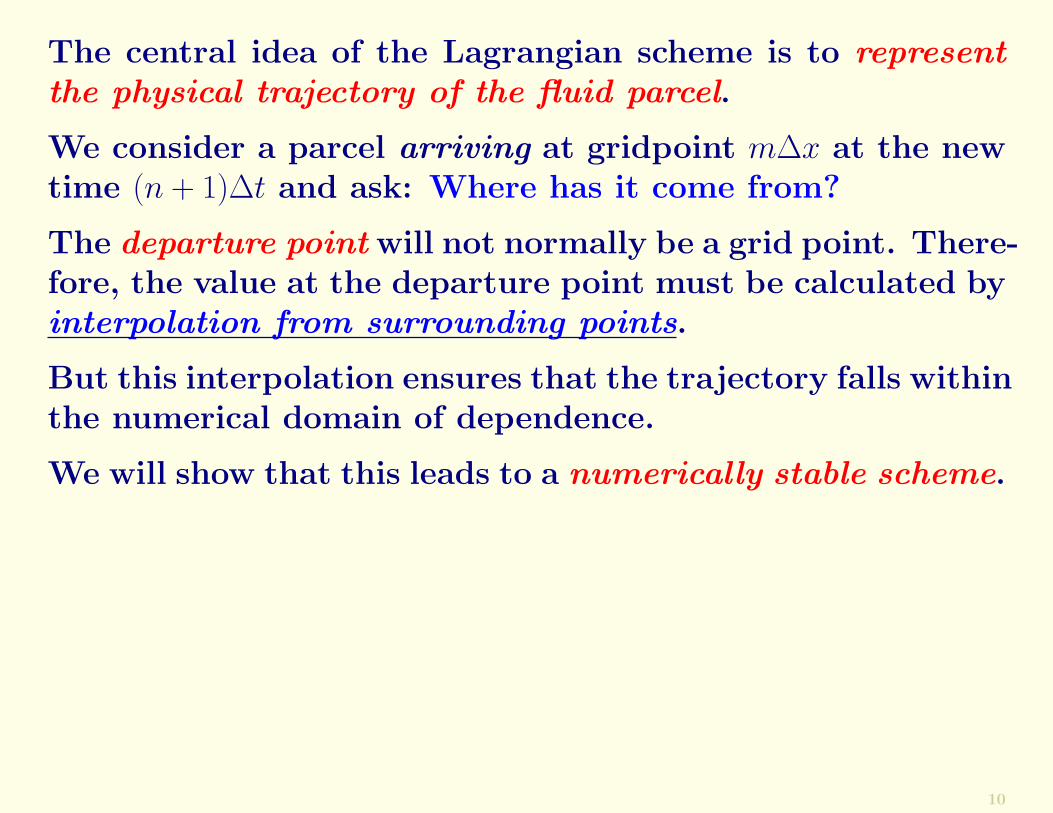
The central idea of the Lagrangian scheme is to representthe physical trajectory of the fluid parcel.

10


We consider a parcel arriving at gridpoint m!x at the newtime (n + 1)!t and ask: Where has it come from?

10



The departure point will not normally be a grid point. There-fore, the value at the departure point must be calculated byinterpolation from surrounding points.

10



The departure point will not normally be a grid point. There-fore, the value at the departure point must be calculated byinterpolation from surrounding points.

But this interpolation ensures that the trajectory falls withinthe numerical domain of dependence.

We will show that this leads to a numerically stable scheme.

10

Interpolation using Surrounding Points

+--------+--------+--------+--------+--------&--------+ n+1| | | | | & | || | | | &| | |+--------+--------+--------+++•++++++--------+--------+ n| | | & | | | || | | & | | | |+--------++++++&+++--------+--------+--------+--------+ n-1| | | | | | |m-5 m-4 m-3 m-2 m-1 m m+1

The line of circles (&) represents a parcel trajectory (c = 5!x3!t )

11


+--------+--------+--------+--------+--------&--------+ n+1| | | | | & | || | | | &| | |+--------+--------+--------+++•++++++--------+--------+ n| | | & | | | || | | & | | | |+--------++++++&+++--------+--------+--------+--------+ n-1| | | | | | |m-5 m-4 m-3 m-2 m-1 m m+1


At time n!t the parcel is at (•), which is not a grid-point.

11


+--------+--------+--------+--------+--------&--------+ n+1| | | | | & | || | | | &| | |+--------+--------+--------+++•++++++--------+--------+ n| | | & | | | || | | & | | | |+--------++++++&+++--------+--------+--------+--------+ n-1| | | | | | |m-5 m-4 m-3 m-2 m-1 m m+1


At time n!t the parcel is at (•), which is not a grid-point.

The value at the departure point is obtained by interpola-tion from surrounding points.

Thus we ensure that, even though µ = 53 > 1, the physical

trajectory is within the domain of numerical dependence.

11

The advection equation in Lagrangian form may be written

dY

dt= 0 .

In physical terms, this equation says that the value of Y isconstant for a fluid parcel.

12


dY

dt= 0 .


Applying the equation over the time interval [n!t, (n+ 1)!t],we get

!

"Value of Y atpoint m!x attime (n + 1)!t

#

$ =

!

"Value of Y at

departure pointat time n!t

#

$

12


dY

dt= 0 .


Applying the equation over the time interval [n!t, (n+ 1)!t],we get

!

"Value of Y atpoint m!x attime (n + 1)!t

#

$ =

!

"Value of Y at

departure pointat time n!t

#

$

In a more compact form, we may write

Y n+1m = Y n

•

where Y n• represents the value at the departure point,

which is normally not a grid point.

12


+--------+--------+--------+--------+--------&--------+ n+1| | | | | & | || | | | &| | |+--------+--------+--------+++•++++++--------+--------+ nm-5 m-4 m-3 m-2 m-1 m m+1

The distance travelled in time !t is s = c!t.

13


+--------+--------+--------+--------+--------&--------+ n+1| | | | | & | || | | | &| | |+--------+--------+--------+++•++++++--------+--------+ nm-5 m-4 m-3 m-2 m-1 m m+1

The distance travelled in time !t is s = c!t.The Courant Number is µ = c!t

!x . Here, µ = 53. We define:

p = [µ] = Integral part of µ$ = µ$ p = Fractional part of µ

Note that, by definition, 0 " $ < 1 (here, p = 1 and $ = 2/3).

13


+--------+--------+--------+--------+--------&--------+ n+1| | | | | & | || | | | &| | |+--------+--------+--------+++•++++++--------+--------+ nm-5 m-4 m-3 m-2 m-1 m m+1




Note that, by definition, 0 " $ < 1 (here, p = 1 and $ = 2/3).So, the departure point falls between the grid pointsm$ p$ 1 and m$ p.

13


+--------+--------+--------+--------+--------&--------+ n+1| | | | | & | || | | | &| | |+--------+--------+--------+++•++++++--------+--------+ nm-5 m-4 m-3 m-2 m-1 m m+1




Note that, by definition, 0 " $ < 1 (here, p = 1 and $ = 2/3).So, the departure point falls between the grid pointsm$ p$ 1 and m$ p.A linear interpolation gives

Y n• = $Y n

m$p$1 + (1$ $)Y nm$p .

13


+--------+--------+--------+--------+--------&--------+ n+1| | | | | & | || | | | &| | |+--------+--------+--------+++•++++++--------+--------+ nm-5 m-4 m-3 m-2 m-1 m m+1




Note that, by definition, 0 " $ < 1 (here, p = 1 and $ = 2/3).So, the departure point falls between the grid pointsm$ p$ 1 and m$ p.A linear interpolation gives

Y n• = $Y n

m$p$1 + (1$ $)Y nm$p .

Check: Show what this implies in the limits $ = 0 and $ ' 1.13

Break here

14

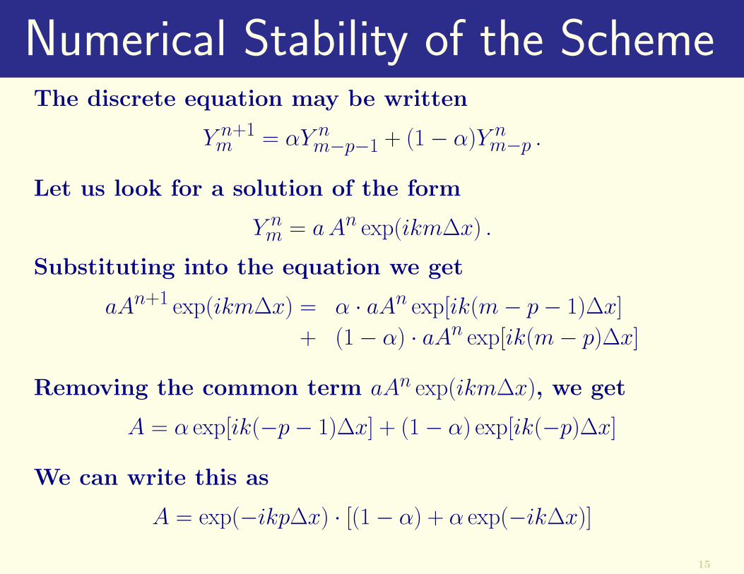
Numerical Stability of the SchemeThe discrete equation may be written

Y n+1m = $Y n

m$p$1 + (1$ $)Y nm$p .

15


Y n+1m = $Y n

m$p$1 + (1$ $)Y nm$p .

Let us look for a solution of the form

Y nm = a An exp(ikm!x) .

15


Y n+1m = $Y n

m$p$1 + (1$ $)Y nm$p .



Substituting into the equation we get

aAn+1 exp(ikm!x) = $ · aAn exp[ik(m$ p$ 1)!x]

+ (1$ $) · aAn exp[ik(m$ p)!x]

15


Y n+1m = $Y n

m$p$1 + (1$ $)Y nm$p .





+ (1$ $) · aAn exp[ik(m$ p)!x]

Removing the common term aAn exp(ikm!x), we get

A = $ exp[ik($p$ 1)!x] + (1$ $) exp[ik($p)!x]

15


Y n+1m = $Y n

m$p$1 + (1$ $)Y nm$p .





+ (1$ $) · aAn exp[ik(m$ p)!x]

Removing the common term aAn exp(ikm!x), we get

A = $ exp[ik($p$ 1)!x] + (1$ $) exp[ik($p)!x]

We can write this as

A = exp($ikp!x) · [(1$ $) + $ exp($ik!x)]

15

Again,

A = exp($ikp!x) · [(1$ $) + $ exp($ik!x)]

16

Again,

A = exp($ikp!x) · [(1$ $) + $ exp($ik!x)]

Now consider the squared modulus of A:

|A|2 = |exp($ikp!x)|2 · |(1$ $) + $ exp($ik!x)|2

= |(1$ $) + $ cos k!x$ i$ sin k!x|2

= [(1$ $) + $ cos k!x]2 + $[sin k!x]2

= (1$ $)2 + 2(1$ $)$ cos k!x + $2 cos2 k!x + $2 sin2 k!x= (1$ 2$ + $2) + 2$(1$ $) cos k!x + $2

= 1$ 2$(1$ $)[1$ cos k!x] .

16

Again,

A = exp($ikp!x) · [(1$ $) + $ exp($ik!x)]


|A|2 = |exp($ikp!x)|2 · |(1$ $) + $ exp($ik!x)|2

= |(1$ $) + $ cos k!x$ i$ sin k!x|2

= [(1$ $) + $ cos k!x]2 + $[sin k!x]2


= 1$ 2$(1$ $)[1$ cos k!x] .

We note that, for all %, we have 0 " (1$ cos %) " 2.

16

Again,

A = exp($ikp!x) · [(1$ $) + $ exp($ik!x)]


|A|2 = |exp($ikp!x)|2 · |(1$ $) + $ exp($ik!x)|2

= |(1$ $) + $ cos k!x$ i$ sin k!x|2

= [(1$ $) + $ cos k!x]2 + $[sin k!x]2


= 1$ 2$(1$ $)[1$ cos k!x] .


Taking the largest value of 1$ cos k!x gives

|A|2 = 1$ 4$(1$ $) = (1$ 2$)2 " 1 .

16

Again,

A = exp($ikp!x) · [(1$ $) + $ exp($ik!x)]


|A|2 = |exp($ikp!x)|2 · |(1$ $) + $ exp($ik!x)|2

= |(1$ $) + $ cos k!x$ i$ sin k!x|2

= [(1$ $) + $ cos k!x]2 + $[sin k!x]2


= 1$ 2$(1$ $)[1$ cos k!x] .



|A|2 = 1$ 4$(1$ $) = (1$ 2$)2 " 1 .

Taking the smallest value of 1$ cos k!x gives

|A|2 = 1 .

16

Again,

A = exp($ikp!x) · [(1$ $) + $ exp($ik!x)]


|A|2 = |exp($ikp!x)|2 · |(1$ $) + $ exp($ik!x)|2

= |(1$ $) + $ cos k!x$ i$ sin k!x|2

= [(1$ $) + $ cos k!x]2 + $[sin k!x]2


= 1$ 2$(1$ $)[1$ cos k!x] .



|A|2 = 1$ 4$(1$ $) = (1$ 2$)2 " 1 .

Taking the smallest value of 1$ cos k!x gives

|A|2 = 1 .

In either case, |A|2 " 1, so there is numerical stability.16

Discussion and Conclusion

17

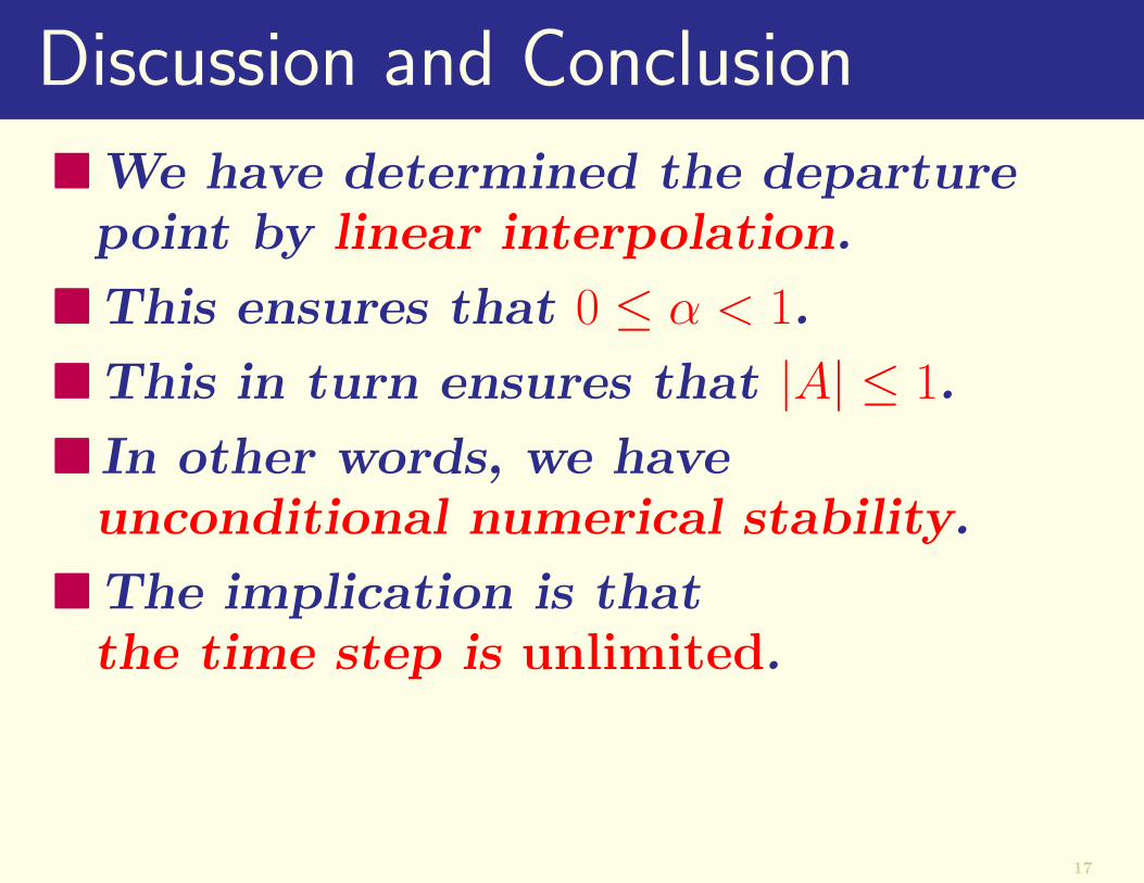
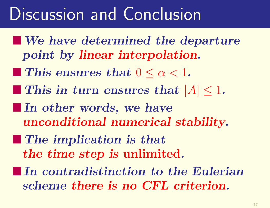
Discussion and Conclusion!We have determined the departure

point by linear interpolation.

17



!This ensures that 0 " $ < 1.

17




!This in turn ensures that |A| " 1.

17





! In other words, we haveunconditional numerical stability.

17






!The implication is thatthe time step is unlimited.

17






!The implication is thatthe time step is unlimited.

! In contradistinction to the Eulerianscheme there is no CFL criterion.

17

!Of course, we must consider accuracyas well as stability

18


!The time step !t is chosen to ensuresu!cient accuracy, but can be muchlarger than for an Eulerian scheme.

18



!Typically, !t is about six times largerfor a semi-Lagrangian scheme than foran Eulerian scheme.

18



!Typically, !t is about six times largerfor a semi-Lagrangian scheme than foran Eulerian scheme.

!This is a substantial gain in computa-tional e!ciency.

& & &

18

Miscellaneous Issues

19

Miscellaneous Issues!Calculation of departure point

19


!Higher order interpolation

19



! Interpolation in two dimensions

19




! Interpolation in the vertical

19





!Coriolis terms: Pseudo-implicit scheme

19





!Coriolis terms: Pseudo-implicit scheme

! Inclusion of Physics

19

End of §3.2.6

20

3.2 .6. Semi -Lag rangi an A dvect ion - UMD | …ekalnay/syllabi/AOSC614/NWP-CH03-2-6.pdf¤3.2 .6. Semi -Lag rangi an A dvect ion ¥ W e ha v e studi ed the Euler ian leapfr o g sc

Documents