3.1 | Demand, Supply, and Equilibrium in Markets for · When the price of gasoline rises, for example, it encourages profit-seeking firms to take several actions: ... Equilibrium—Where

• Price Ceilings and Price Floors

An auction bidder pays thousands of dollars for a dress Whitney Houston wore. A collector spends a small fortunefor a few drawings by John Lennon. People usually react to purchases like these in two ways: their jaw drops becausethey think these are high prices to pay for such goods or they think these are rare, desirable items and the amount paidseems right.

Visit this website (http://openstaxcollege.org/l/celebauction) to read a list of bizarre items that have beenpurchased for their ties to celebrities. These examples represent an interesting facet of demand and supply.

When economists talk about prices, they are less interested in making judgments than in gaining a practicalunderstanding of what determines prices and why prices change. Consider a price most of us contend with weekly:that of a gallon of gas. Why was the average price of gasoline in the United States $3.71 per gallon in June 2014?Why did the price for gasoline fall sharply to $2.07 per gallon by January 2015? To explain these price movements,economists focus on the determinants of what gasoline buyers are willing to pay and what gasoline sellers are willingto accept.

As it turns out, the price of gasoline in June of any given year is nearly always higher than the price in January of thatsame year; over recent decades, gasoline prices in midsummer have averaged about 10 cents per gallon more thantheir midwinter low. The likely reason is that people drive more in the summer, and are also willing to pay more forgas, but that does not explain how steeply gas prices fell. Other factors were at work during those six months, such asincreases in supply and decreases in the demand for crude oil.

This chapter introduces the economic model of demand and supply—one of the most powerful models in all ofeconomics. The discussion here begins by examining how demand and supply determine the price and the quantitysold in markets for goods and services, and how changes in demand and supply lead to changes in prices andquantities.

3.1 | Demand, Supply, and Equilibrium in Markets for

Goods and Services

By the end of this section, you will be able to:• Explain demand, quantity demanded, and the law of demand• Identify a demand curve and a supply curve• Explain supply, quantity supply, and the law of supply• Explain equilibrium, equilibrium price, and equilibrium quantity

First let’s first focus on what economists mean by demand, what they mean by supply, and then how demand andsupply interact in a market.

46 Chapter 3 | Demand and Supply

This OpenStax book is available for free at http://cnx.org/content/col11613/1.11

http://openstaxcollege.org/l/celebauction

Demand for Goods and ServicesEconomists use the term demand to refer to the amount of some good or service consumers are willing and able topurchase at each price. Demand is based on needs and wants—a consumer may be able to differentiate between aneed and a want, but from an economist’s perspective they are the same thing. Demand is also based on ability to pay.If you cannot pay for it, you have no effective demand.

What a buyer pays for a unit of the specific good or service is called price. The total number of units purchased atthat price is called the quantity demanded. A rise in price of a good or service almost always decreases the quantitydemanded of that good or service. Conversely, a fall in price will increase the quantity demanded. When the price ofa gallon of gasoline goes up, for example, people look for ways to reduce their consumption by combining severalerrands, commuting by carpool or mass transit, or taking weekend or vacation trips closer to home. Economists callthis inverse relationship between price and quantity demanded the law of demand. The law of demand assumes thatall other variables that affect demand (to be explained in the next module) are held constant.

An example from the market for gasoline can be shown in the form of a table or a graph. A table that shows thequantity demanded at each price, such as Table 3.1, is called a demand schedule. Price in this case is measured indollars per gallon of gasoline. The quantity demanded is measured in millions of gallons over some time period (forexample, per day or per year) and over some geographic area (like a state or a country). A demand curve shows therelationship between price and quantity demanded on a graph like Figure 3.2, with quantity on the horizontal axisand the price per gallon on the vertical axis. (Note that this is an exception to the normal rule in mathematics that theindependent variable (x) goes on the horizontal axis and the dependent variable (y) goes on the vertical. Economicsis not math.)

The demand schedule shown by Table 3.1 and the demand curve shown by the graph in Figure 3.2 are two ways ofdescribing the same relationship between price and quantity demanded.

Figure 3.2 A Demand Curve for Gasoline The demand schedule shows that as price rises, quantity demandeddecreases, and vice versa. These points are then graphed, and the line connecting them is the demand curve (D).The downward slope of the demand curve again illustrates the law of demand—the inverse relationship betweenprices and quantity demanded.

Price (per gallon) Quantity Demanded (millions of gallons)

$1.00 800

$1.20 700

$1.40 600

Table 3.1 Price and Quantity Demanded of Gasoline

Chapter 3 | Demand and Supply 47

Price (per gallon) Quantity Demanded (millions of gallons)

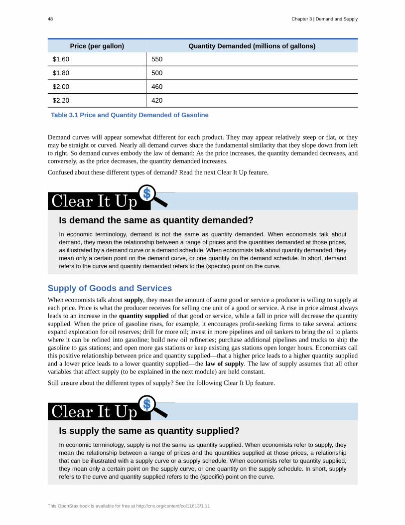
$1.60 550

$1.80 500

$2.00 460

$2.20 420

Table 3.1 Price and Quantity Demanded of Gasoline

Demand curves will appear somewhat different for each product. They may appear relatively steep or flat, or theymay be straight or curved. Nearly all demand curves share the fundamental similarity that they slope down from leftto right. So demand curves embody the law of demand: As the price increases, the quantity demanded decreases, andconversely, as the price decreases, the quantity demanded increases.

Confused about these different types of demand? Read the next Clear It Up feature.

Is demand the same as quantity demanded?

In economic terminology, demand is not the same as quantity demanded. When economists talk aboutdemand, they mean the relationship between a range of prices and the quantities demanded at those prices,as illustrated by a demand curve or a demand schedule. When economists talk about quantity demanded, theymean only a certain point on the demand curve, or one quantity on the demand schedule. In short, demandrefers to the curve and quantity demanded refers to the (specific) point on the curve.

Supply of Goods and ServicesWhen economists talk about supply, they mean the amount of some good or service a producer is willing to supply ateach price. Price is what the producer receives for selling one unit of a good or service. A rise in price almost alwaysleads to an increase in the quantity supplied of that good or service, while a fall in price will decrease the quantitysupplied. When the price of gasoline rises, for example, it encourages profit-seeking firms to take several actions:expand exploration for oil reserves; drill for more oil; invest in more pipelines and oil tankers to bring the oil to plantswhere it can be refined into gasoline; build new oil refineries; purchase additional pipelines and trucks to ship thegasoline to gas stations; and open more gas stations or keep existing gas stations open longer hours. Economists callthis positive relationship between price and quantity supplied—that a higher price leads to a higher quantity suppliedand a lower price leads to a lower quantity supplied—the law of supply. The law of supply assumes that all othervariables that affect supply (to be explained in the next module) are held constant.

Still unsure about the different types of supply? See the following Clear It Up feature.

Is supply the same as quantity supplied?

In economic terminology, supply is not the same as quantity supplied. When economists refer to supply, theymean the relationship between a range of prices and the quantities supplied at those prices, a relationshipthat can be illustrated with a supply curve or a supply schedule. When economists refer to quantity supplied,they mean only a certain point on the supply curve, or one quantity on the supply schedule. In short, supplyrefers to the curve and quantity supplied refers to the (specific) point on the curve.



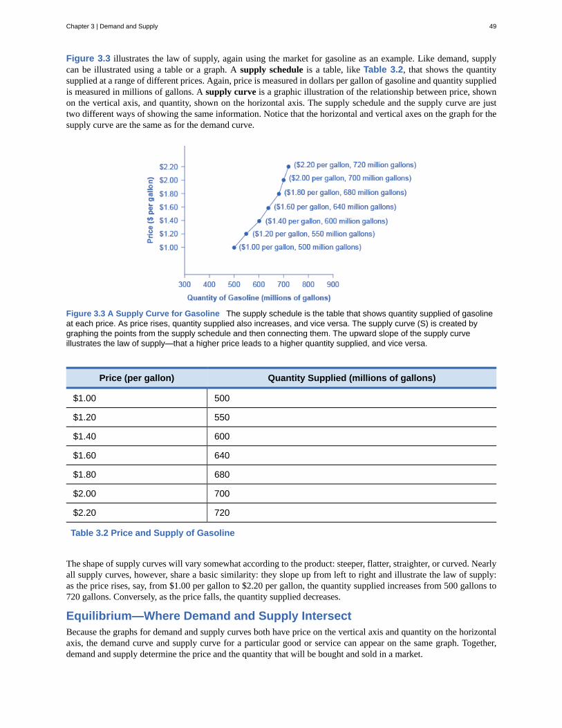
Figure 3.3 illustrates the law of supply, again using the market for gasoline as an example. Like demand, supplycan be illustrated using a table or a graph. A supply schedule is a table, like Table 3.2, that shows the quantitysupplied at a range of different prices. Again, price is measured in dollars per gallon of gasoline and quantity suppliedis measured in millions of gallons. A supply curve is a graphic illustration of the relationship between price, shownon the vertical axis, and quantity, shown on the horizontal axis. The supply schedule and the supply curve are justtwo different ways of showing the same information. Notice that the horizontal and vertical axes on the graph for thesupply curve are the same as for the demand curve.

Figure 3.3 A Supply Curve for Gasoline The supply schedule is the table that shows quantity supplied of gasolineat each price. As price rises, quantity supplied also increases, and vice versa. The supply curve (S) is created bygraphing the points from the supply schedule and then connecting them. The upward slope of the supply curveillustrates the law of supply—that a higher price leads to a higher quantity supplied, and vice versa.

Price (per gallon) Quantity Supplied (millions of gallons)

$1.00 500

$1.20 550

$1.40 600

$1.60 640

$1.80 680

$2.00 700

$2.20 720

Table 3.2 Price and Supply of Gasoline

The shape of supply curves will vary somewhat according to the product: steeper, flatter, straighter, or curved. Nearlyall supply curves, however, share a basic similarity: they slope up from left to right and illustrate the law of supply:as the price rises, say, from $1.00 per gallon to $2.20 per gallon, the quantity supplied increases from 500 gallons to720 gallons. Conversely, as the price falls, the quantity supplied decreases.

Equilibrium—Where Demand and Supply IntersectBecause the graphs for demand and supply curves both have price on the vertical axis and quantity on the horizontalaxis, the demand curve and supply curve for a particular good or service can appear on the same graph. Together,demand and supply determine the price and the quantity that will be bought and sold in a market.


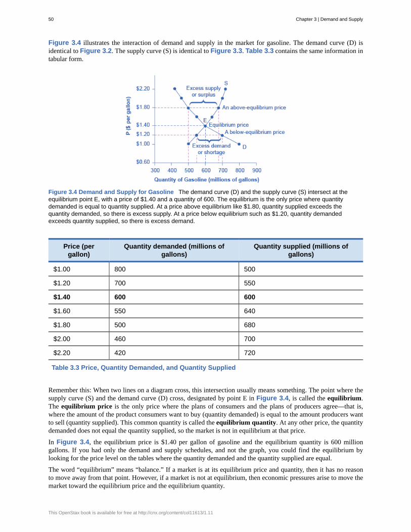
Figure 3.4 illustrates the interaction of demand and supply in the market for gasoline. The demand curve (D) isidentical to Figure 3.2. The supply curve (S) is identical to Figure 3.3. Table 3.3 contains the same information intabular form.

Figure 3.4 Demand and Supply for Gasoline The demand curve (D) and the supply curve (S) intersect at theequilibrium point E, with a price of $1.40 and a quantity of 600. The equilibrium is the only price where quantitydemanded is equal to quantity supplied. At a price above equilibrium like $1.80, quantity supplied exceeds thequantity demanded, so there is excess supply. At a price below equilibrium such as $1.20, quantity demandedexceeds quantity supplied, so there is excess demand.

Price (pergallon)

Quantity demanded (millions ofgallons)

Quantity supplied (millions ofgallons)

$1.00 800 500

$1.20 700 550

$1.40 600 600

$1.60 550 640

$1.80 500 680

$2.00 460 700

$2.20 420 720

Table 3.3 Price, Quantity Demanded, and Quantity Supplied

Remember this: When two lines on a diagram cross, this intersection usually means something. The point where thesupply curve (S) and the demand curve (D) cross, designated by point E in Figure 3.4, is called the equilibrium.The equilibrium price is the only price where the plans of consumers and the plans of producers agree—that is,where the amount of the product consumers want to buy (quantity demanded) is equal to the amount producers wantto sell (quantity supplied). This common quantity is called the equilibrium quantity. At any other price, the quantitydemanded does not equal the quantity supplied, so the market is not in equilibrium at that price.

In Figure 3.4, the equilibrium price is $1.40 per gallon of gasoline and the equilibrium quantity is 600 milliongallons. If you had only the demand and supply schedules, and not the graph, you could find the equilibrium bylooking for the price level on the tables where the quantity demanded and the quantity supplied are equal.

The word “equilibrium” means “balance.” If a market is at its equilibrium price and quantity, then it has no reasonto move away from that point. However, if a market is not at equilibrium, then economic pressures arise to move themarket toward the equilibrium price and the equilibrium quantity.



Imagine, for example, that the price of a gallon of gasoline was above the equilibrium price—that is, instead of $1.40per gallon, the price is $1.80 per gallon. This above-equilibrium price is illustrated by the dashed horizontal line atthe price of $1.80 in Figure 3.4. At this higher price, the quantity demanded drops from 600 to 500. This decline inquantity reflects how consumers react to the higher price by finding ways to use less gasoline.

Moreover, at this higher price of $1.80, the quantity of gasoline supplied rises from the 600 to 680, as the higherprice makes it more profitable for gasoline producers to expand their output. Now, consider how quantity demandedand quantity supplied are related at this above-equilibrium price. Quantity demanded has fallen to 500 gallons, whilequantity supplied has risen to 680 gallons. In fact, at any above-equilibrium price, the quantity supplied exceeds thequantity demanded. We call this an excess supply or a surplus.

With a surplus, gasoline accumulates at gas stations, in tanker trucks, in pipelines, and at oil refineries. Thisaccumulation puts pressure on gasoline sellers. If a surplus remains unsold, those firms involved in making andselling gasoline are not receiving enough cash to pay their workers and to cover their expenses. In this situation, someproducers and sellers will want to cut prices, because it is better to sell at a lower price than not to sell at all. Oncesome sellers start cutting prices, others will follow to avoid losing sales. These price reductions in turn will stimulate ahigher quantity demanded. So, if the price is above the equilibrium level, incentives built into the structure of demandand supply will create pressures for the price to fall toward the equilibrium.

Now suppose that the price is below its equilibrium level at $1.20 per gallon, as the dashed horizontal line at thisprice in Figure 3.4 shows. At this lower price, the quantity demanded increases from 600 to 700 as drivers takelonger trips, spend more minutes warming up the car in the driveway in wintertime, stop sharing rides to work, andbuy larger cars that get fewer miles to the gallon. However, the below-equilibrium price reduces gasoline producers’incentives to produce and sell gasoline, and the quantity supplied falls from 600 to 550.

When the price is below equilibrium, there is excess demand, or a shortage—that is, at the given price the quantitydemanded, which has been stimulated by the lower price, now exceeds the quantity supplied, which had beendepressed by the lower price. In this situation, eager gasoline buyers mob the gas stations, only to find many stationsrunning short of fuel. Oil companies and gas stations recognize that they have an opportunity to make higher profitsby selling what gasoline they have at a higher price. As a result, the price rises toward the equilibrium level.Read Demand, Supply, and Efficiency (http://cnx.org/content/m48832/latest/) for more discussion on theimportance of the demand and supply model.

3.2 | Shifts in Demand and Supply for Goods and

Services

By the end of this section, you will be able to:• Identify factors that affect demand• Graph demand curves and demand shifts• Identify factors that affect supply• Graph supply curves and supply shifts

The previous module explored how price affects the quantity demanded and the quantity supplied. The result was thedemand curve and the supply curve. Price, however, is not the only thing that influences demand. Nor is it the onlything that influences supply. For example, how is demand for vegetarian food affected if, say, health concerns causemore consumers to avoid eating meat? Or how is the supply of diamonds affected if diamond producers discoverseveral new diamond mines? What are the major factors, in addition to the price, that influence demand or supply?

Visit this website (http://openstaxcollege.org/l/toothfish) to read a brief note on how marketing strategies caninfluence supply and demand of products.


http://cnx.org/content/m48832/latest/

http://openstaxcollege.org/l/toothfish

What Factors Affect Demand?We defined demand as the amount of some product a consumer is willing and able to purchase at each price. Thatsuggests at least two factors in addition to price that affect demand. Willingness to purchase suggests a desire, basedon what economists call tastes and preferences. If you neither need nor want something, you will not buy it. Abilityto purchase suggests that income is important. Professors are usually able to afford better housing and transportationthan students, because they have more income. Prices of related goods can affect demand also. If you need a newcar, the price of a Honda may affect your demand for a Ford. Finally, the size or composition of the population canaffect demand. The more children a family has, the greater their demand for clothing. The more driving-age childrena family has, the greater their demand for car insurance, and the less for diapers and baby formula.

These factors matter both for demand by an individual and demand by the market as a whole. Exactly how do thesevarious factors affect demand, and how do we show the effects graphically? To answer those questions, we need theceteris paribus assumption.

The Ceteris Paribus AssumptionA demand curve or a supply curve is a relationship between two, and only two, variables: quantity on the horizontalaxis and price on the vertical axis. The assumption behind a demand curve or a supply curve is that no relevanteconomic factors, other than the product’s price, are changing. Economists call this assumption ceteris paribus, aLatin phrase meaning “other things being equal.” Any given demand or supply curve is based on the ceteris paribusassumption that all else is held equal. A demand curve or a supply curve is a relationship between two, and only two,variables when all other variables are kept constant. If all else is not held equal, then the laws of supply and demandwill not necessarily hold, as the following Clear It Up feature shows.

When does ceteris paribus apply?

Ceteris paribus is typically applied when we look at how changes in price affect demand or supply, but ceterisparibus can be applied more generally. In the real world, demand and supply depend on more factors than justprice. For example, a consumer’s demand depends on income and a producer’s supply depends on the costof producing the product. How can we analyze the effect on demand or supply if multiple factors are changingat the same time—say price rises and income falls? The answer is that we examine the changes one at atime, assuming the other factors are held constant.

For example, we can say that an increase in the price reduces the amount consumers will buy (assumingincome, and anything else that affects demand, is unchanged). Additionally, a decrease in income reduces theamount consumers can afford to buy (assuming price, and anything else that affects demand, is unchanged).This is what the ceteris paribus assumption really means. In this particular case, after we analyze each factorseparately, we can combine the results. The amount consumers buy falls for two reasons: first because of thehigher price and second because of the lower income.



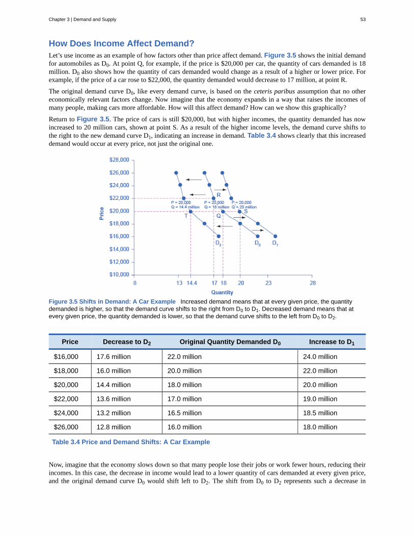
How Does Income Affect Demand?Let’s use income as an example of how factors other than price affect demand. Figure 3.5 shows the initial demandfor automobiles as D0. At point Q, for example, if the price is $20,000 per car, the quantity of cars demanded is 18million. D0 also shows how the quantity of cars demanded would change as a result of a higher or lower price. Forexample, if the price of a car rose to $22,000, the quantity demanded would decrease to 17 million, at point R.

The original demand curve D0, like every demand curve, is based on the ceteris paribus assumption that no othereconomically relevant factors change. Now imagine that the economy expands in a way that raises the incomes ofmany people, making cars more affordable. How will this affect demand? How can we show this graphically?

Return to Figure 3.5. The price of cars is still $20,000, but with higher incomes, the quantity demanded has nowincreased to 20 million cars, shown at point S. As a result of the higher income levels, the demand curve shifts tothe right to the new demand curve D1, indicating an increase in demand. Table 3.4 shows clearly that this increaseddemand would occur at every price, not just the original one.

Figure 3.5 Shifts in Demand: A Car Example Increased demand means that at every given price, the quantitydemanded is higher, so that the demand curve shifts to the right from D0 to D1. Decreased demand means that atevery given price, the quantity demanded is lower, so that the demand curve shifts to the left from D0 to D2.

Price Decrease to D2 Original Quantity Demanded D0 Increase to D1

$16,000 17.6 million 22.0 million 24.0 million






Table 3.4 Price and Demand Shifts: A Car Example

Now, imagine that the economy slows down so that many people lose their jobs or work fewer hours, reducing theirincomes. In this case, the decrease in income would lead to a lower quantity of cars demanded at every given price,and the original demand curve D0 would shift left to D2. The shift from D0 to D2 represents such a decrease in


demand: At any given price level, the quantity demanded is now lower. In this example, a price of $20,000 means 18million cars sold along the original demand curve, but only 14.4 million sold after demand fell.

When a demand curve shifts, it does not mean that the quantity demanded by every individual buyer changes by thesame amount. In this example, not everyone would have higher or lower income and not everyone would buy or notbuy an additional car. Instead, a shift in a demand curve captures an pattern for the market as a whole.

In the previous section, we argued that higher income causes greater demand at every price. This is true for mostgoods and services. For some—luxury cars, vacations in Europe, and fine jewelry—the effect of a rise in income canbe especially pronounced. A product whose demand rises when income rises, and vice versa, is called a normal good.A few exceptions to this pattern do exist. As incomes rise, many people will buy fewer generic brand groceries andmore name brand groceries. They are less likely to buy used cars and more likely to buy new cars. They will be lesslikely to rent an apartment and more likely to own a home, and so on. A product whose demand falls when incomerises, and vice versa, is called an inferior good. In other words, when income increases, the demand curve shifts tothe left.

Other Factors That Shift Demand CurvesIncome is not the only factor that causes a shift in demand. Other things that change demand include tastes andpreferences, the composition or size of the population, the prices of related goods, and even expectations. A changein any one of the underlying factors that determine what quantity people are willing to buy at a given price will causea shift in demand. Graphically, the new demand curve lies either to the right (an increase) or to the left (a decrease)of the original demand curve. Let’s look at these factors.

Changing Tastes or Preferences

From 1980 to 2014, the per-person consumption of chicken by Americans rose from 48 pounds per year to 85pounds per year, and consumption of beef fell from 77 pounds per year to 54 pounds per year, according to the U.S.Department of Agriculture (USDA). Changes like these are largely due to movements in taste, which change thequantity of a good demanded at every price: that is, they shift the demand curve for that good, rightward for chickenand leftward for beef.

Changes in the Composition of the Population

The proportion of elderly citizens in the United States population is rising. It rose from 9.8% in 1970 to 12.6% in2000, and will be a projected (by the U.S. Census Bureau) 20% of the population by 2030. A society with relativelymore children, like the United States in the 1960s, will have greater demand for goods and services like tricycles andday care facilities. A society with relatively more elderly persons, as the United States is projected to have by 2030,has a higher demand for nursing homes and hearing aids. Similarly, changes in the size of the population can affect thedemand for housing and many other goods. Each of these changes in demand will be shown as a shift in the demandcurve.

The demand for a product can also be affected by changes in the prices of related goods such as substitutes orcomplements. A substitute is a good or service that can be used in place of another good or service. As electronicbooks, like this one, become more available, you would expect to see a decrease in demand for traditional printedbooks. A lower price for a substitute decreases demand for the other product. For example, in recent years as the priceof tablet computers has fallen, the quantity demanded has increased (because of the law of demand). Since people arepurchasing tablets, there has been a decrease in demand for laptops, which can be shown graphically as a leftwardshift in the demand curve for laptops. A higher price for a substitute good has the reverse effect.

Other goods are complements for each other, meaning that the goods are often used together, because consumptionof one good tends to enhance consumption of the other. Examples include breakfast cereal and milk; notebooks andpens or pencils, golf balls and golf clubs; gasoline and sport utility vehicles; and the five-way combination of bacon,lettuce, tomato, mayonnaise, and bread. If the price of golf clubs rises, since the quantity demanded of golf clubs falls(because of the law of demand), demand for a complement good like golf balls decreases, too. Similarly, a higherprice for skis would shift the demand curve for a complement good like ski resort trips to the left, while a lower pricefor a complement has the reverse effect.

Changes in Expectations about Future Prices or Other Factors that Affect Demand

While it is clear that the price of a good affects the quantity demanded, it is also true that expectations about the futureprice (or expectations about tastes and preferences, income, and so on) can affect demand. For example, if peoplehear that a hurricane is coming, they may rush to the store to buy flashlight batteries and bottled water. If people learn



that the price of a good like coffee is likely to rise in the future, they may head for the store to stock up on coffeenow. These changes in demand are shown as shifts in the curve. Therefore, a shift in demand happens when a changein some economic factor (other than price) causes a different quantity to be demanded at every price. The followingWork It Out feature shows how this happens.

Shift in Demand

A shift in demand means that at any price (and at every price), the quantity demanded will be different than itwas before. Following is an example of a shift in demand due to an income increase.

Step 1. Draw the graph of a demand curve for a normal good like pizza. Pick a price (like P0). Identify thecorresponding Q0. An example is shown in Figure 3.6.

Figure 3.6 Demand Curve The demand curve can be used to identify how much consumers would buy atany given price.

Step 2. Suppose income increases. As a result of the change, are consumers going to buy more or lesspizza? The answer is more. Draw a dotted horizontal line from the chosen price, through the original quantitydemanded, to the new point with the new Q1. Draw a dotted vertical line down to the horizontal axis and labelthe new Q1. An example is provided in Figure 3.7.

Figure 3.7 Demand Curve with Income Increase With an increase in income, consumers will purchaselarger quantities, pushing demand to the right.

Step 3. Now, shift the curve through the new point. You will see that an increase in income causes an upward(or rightward) shift in the demand curve, so that at any price the quantities demanded will be higher, as shownin Figure 3.8.


Figure 3.8 Demand Curve Shifted Right With an increase in income, consumers will purchase largerquantities, pushing demand to the right, and causing the demand curve to shift right.

Summing Up Factors That Change DemandSix factors that can shift demand curves are summarized in Figure 3.9. The direction of the arrows indicates whetherthe demand curve shifts represent an increase in demand or a decrease in demand. Notice that a change in the price ofthe good or service itself is not listed among the factors that can shift a demand curve. A change in the price of a goodor service causes a movement along a specific demand curve, and it typically leads to some change in the quantitydemanded, but it does not shift the demand curve.

Figure 3.9 Factors That Shift Demand Curves (a) A list of factors that can cause an increase in demand from D0to D1. (b) The same factors, if their direction is reversed, can cause a decrease in demand from D0 to D1.

When a demand curve shifts, it will then intersect with a given supply curve at a different equilibrium priceand quantity. We are, however, getting ahead of our story. Before discussing how changes in demand can affectequilibrium price and quantity, we first need to discuss shifts in supply curves.

How Production Costs Affect SupplyA supply curve shows how quantity supplied will change as the price rises and falls, assuming ceteris paribus so thatno other economically relevant factors are changing. If other factors relevant to supply do change, then the entiresupply curve will shift. Just as a shift in demand is represented by a change in the quantity demanded at every price,a shift in supply means a change in the quantity supplied at every price.

In thinking about the factors that affect supply, remember what motivates firms: profits, which are the differencebetween revenues and costs. Goods and services are produced using combinations of labor, materials, and machinery,or what we call inputs or factors of production. If a firm faces lower costs of production, while the prices for thegood or service the firm produces remain unchanged, a firm’s profits go up. When a firm’s profits increase, it is moremotivated to produce output, since the more it produces the more profit it will earn. So, when costs of production fall,



a firm will tend to supply a larger quantity at any given price for its output. This can be shown by the supply curveshifting to the right.

Take, for example, a messenger company that delivers packages around a city. The company may find that buyinggasoline is one of its main costs. If the price of gasoline falls, then the company will find it can deliver messages morecheaply than before. Since lower costs correspond to higher profits, the messenger company may now supply moreof its services at any given price. For example, given the lower gasoline prices, the company can now serve a greaterarea, and increase its supply.

Conversely, if a firm faces higher costs of production, then it will earn lower profits at any given selling price for itsproducts. As a result, a higher cost of production typically causes a firm to supply a smaller quantity at any givenprice. In this case, the supply curve shifts to the left.

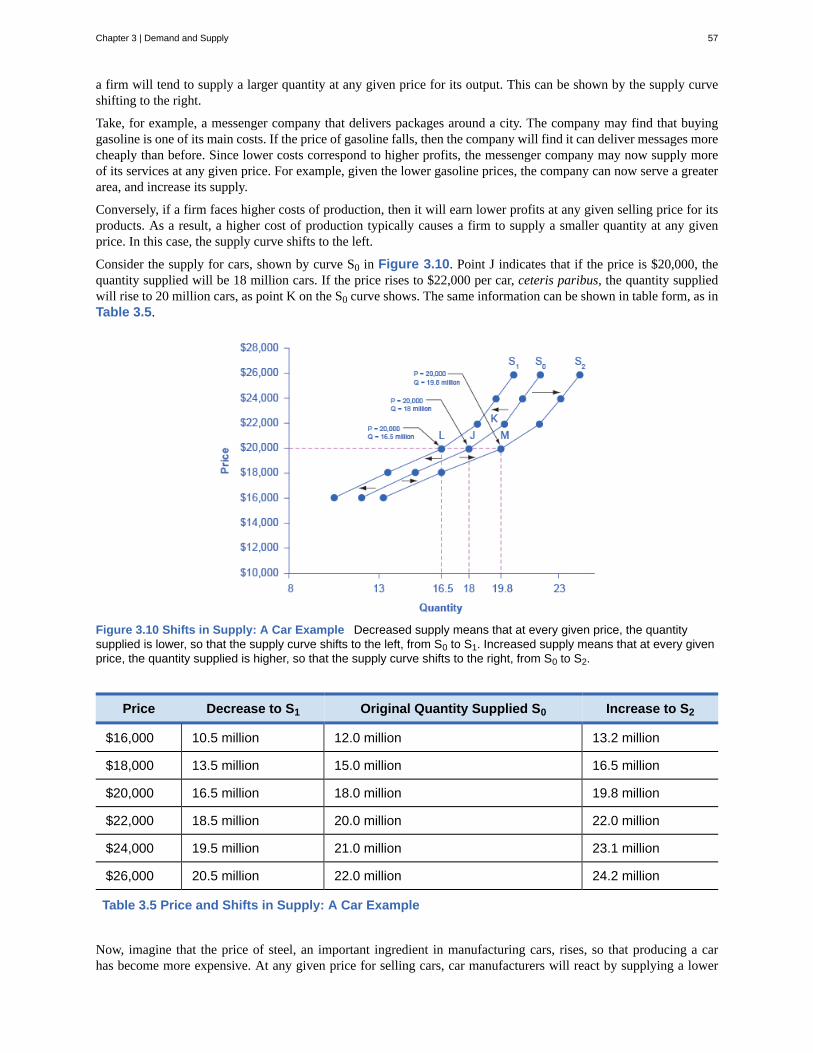
Consider the supply for cars, shown by curve S0 in Figure 3.10. Point J indicates that if the price is $20,000, thequantity supplied will be 18 million cars. If the price rises to $22,000 per car, ceteris paribus, the quantity suppliedwill rise to 20 million cars, as point K on the S0 curve shows. The same information can be shown in table form, as inTable 3.5.

Figure 3.10 Shifts in Supply: A Car Example Decreased supply means that at every given price, the quantitysupplied is lower, so that the supply curve shifts to the left, from S0 to S1. Increased supply means that at every givenprice, the quantity supplied is higher, so that the supply curve shifts to the right, from S0 to S2.

Price Decrease to S1 Original Quantity Supplied S0 Increase to S2







Table 3.5 Price and Shifts in Supply: A Car Example

Now, imagine that the price of steel, an important ingredient in manufacturing cars, rises, so that producing a carhas become more expensive. At any given price for selling cars, car manufacturers will react by supplying a lower


quantity. This can be shown graphically as a leftward shift of supply, from S0 to S1, which indicates that at any givenprice, the quantity supplied decreases. In this example, at a price of $20,000, the quantity supplied decreases from 18million on the original supply curve (S0) to 16.5 million on the supply curve S1, which is labeled as point L.

Conversely, if the price of steel decreases, producing a car becomes less expensive. At any given price for selling cars,car manufacturers can now expect to earn higher profits, so they will supply a higher quantity. The shift of supplyto the right, from S0 to S2, means that at all prices, the quantity supplied has increased. In this example, at a priceof $20,000, the quantity supplied increases from 18 million on the original supply curve (S0) to 19.8 million on thesupply curve S2, which is labeled M.

Other Factors That Affect SupplyIn the example above, we saw that changes in the prices of inputs in the production process will affect the cost ofproduction and thus the supply. Several other things affect the cost of production, too, such as changes in weather orother natural conditions, new technologies for production, and some government policies.

The cost of production for many agricultural products will be affected by changes in natural conditions. For example,in 2014 the Manchurian Plain in Northeastern China, which produces most of the country's wheat, corn, and soybeans,experienced its most severe drought in 50 years. A drought decreases the supply of agricultural products, which meansthat at any given price, a lower quantity will be supplied; conversely, especially good weather would shift the supplycurve to the right.

When a firm discovers a new technology that allows the firm to produce at a lower cost, the supply curve will shiftto the right, as well. For instance, in the 1960s a major scientific effort nicknamed the Green Revolution focused onbreeding improved seeds for basic crops like wheat and rice. By the early 1990s, more than two-thirds of the wheatand rice in low-income countries around the world was grown with these Green Revolution seeds—and the harvestwas twice as high per acre. A technological improvement that reduces costs of production will shift supply to theright, so that a greater quantity will be produced at any given price.

Government policies can affect the cost of production and the supply curve through taxes, regulations, and subsidies.For example, the U.S. government imposes a tax on alcoholic beverages that collects about $8 billion per year fromproducers. Taxes are treated as costs by businesses. Higher costs decrease supply for the reasons discussed above.Other examples of policy that can affect cost are the wide array of government regulations that require firms to spendmoney to provide a cleaner environment or a safer workplace; complying with regulations increases costs.

A government subsidy, on the other hand, is the opposite of a tax. A subsidy occurs when the government pays afirm directly or reduces the firm’s taxes if the firm carries out certain actions. From the firm’s perspective, taxes orregulations are an additional cost of production that shifts supply to the left, leading the firm to produce a lowerquantity at every given price. Government subsidies reduce the cost of production and increase supply at every givenprice, shifting supply to the right. The following Work It Out feature shows how this shift happens.

Shift in Supply

We know that a supply curve shows the minimum price a firm will accept to produce a given quantity of output.What happens to the supply curve when the cost of production goes up? Following is an example of a shift insupply due to a production cost increase.

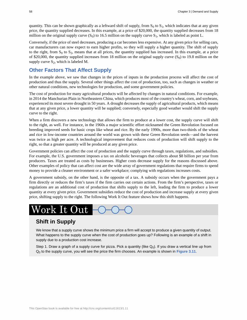
Step 1. Draw a graph of a supply curve for pizza. Pick a quantity (like Q0). If you draw a vertical line up fromQ0 to the supply curve, you will see the price the firm chooses. An example is shown in Figure 3.11.



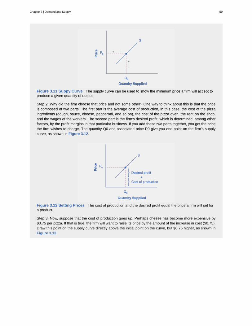
Figure 3.11 Suppy Curve The supply curve can be used to show the minimum price a firm will accept toproduce a given quantity of output.

Step 2. Why did the firm choose that price and not some other? One way to think about this is that the priceis composed of two parts. The first part is the average cost of production, in this case, the cost of the pizzaingredients (dough, sauce, cheese, pepperoni, and so on), the cost of the pizza oven, the rent on the shop,and the wages of the workers. The second part is the firm’s desired profit, which is determined, among otherfactors, by the profit margins in that particular business. If you add these two parts together, you get the pricethe firm wishes to charge. The quantity Q0 and associated price P0 give you one point on the firm’s supplycurve, as shown in Figure 3.12.

Figure 3.12 Setting Prices The cost of production and the desired profit equal the price a firm will set fora product.

Step 3. Now, suppose that the cost of production goes up. Perhaps cheese has become more expensive by$0.75 per pizza. If that is true, the firm will want to raise its price by the amount of the increase in cost ($0.75).Draw this point on the supply curve directly above the initial point on the curve, but $0.75 higher, as shown inFigure 3.13.


Figure 3.13 Increasing Costs Leads to Increasing Price Because the cost of production and thedesired profit equal the price a firm will set for a product, if the cost of production increases, the price for theproduct will also need to increase.

Step 4. Shift the supply curve through this point. You will see that an increase in cost causes an upward (ora leftward) shift of the supply curve so that at any price, the quantities supplied will be smaller, as shown inFigure 3.14.

Figure 3.14 Supply Curve Shifts When the cost of production increases, the supply curve shiftsupwardly to a new price level.

Summing Up Factors That Change SupplyChanges in the cost of inputs, natural disasters, new technologies, and the impact of government decisions all affectthe cost of production. In turn, these factors affect how much firms are willing to supply at any given price.

Figure 3.15 summarizes factors that change the supply of goods and services. Notice that a change in the price ofthe product itself is not among the factors that shift the supply curve. Although a change in price of a good or servicetypically causes a change in quantity supplied or a movement along the supply curve for that specific good or service,it does not cause the supply curve itself to shift.



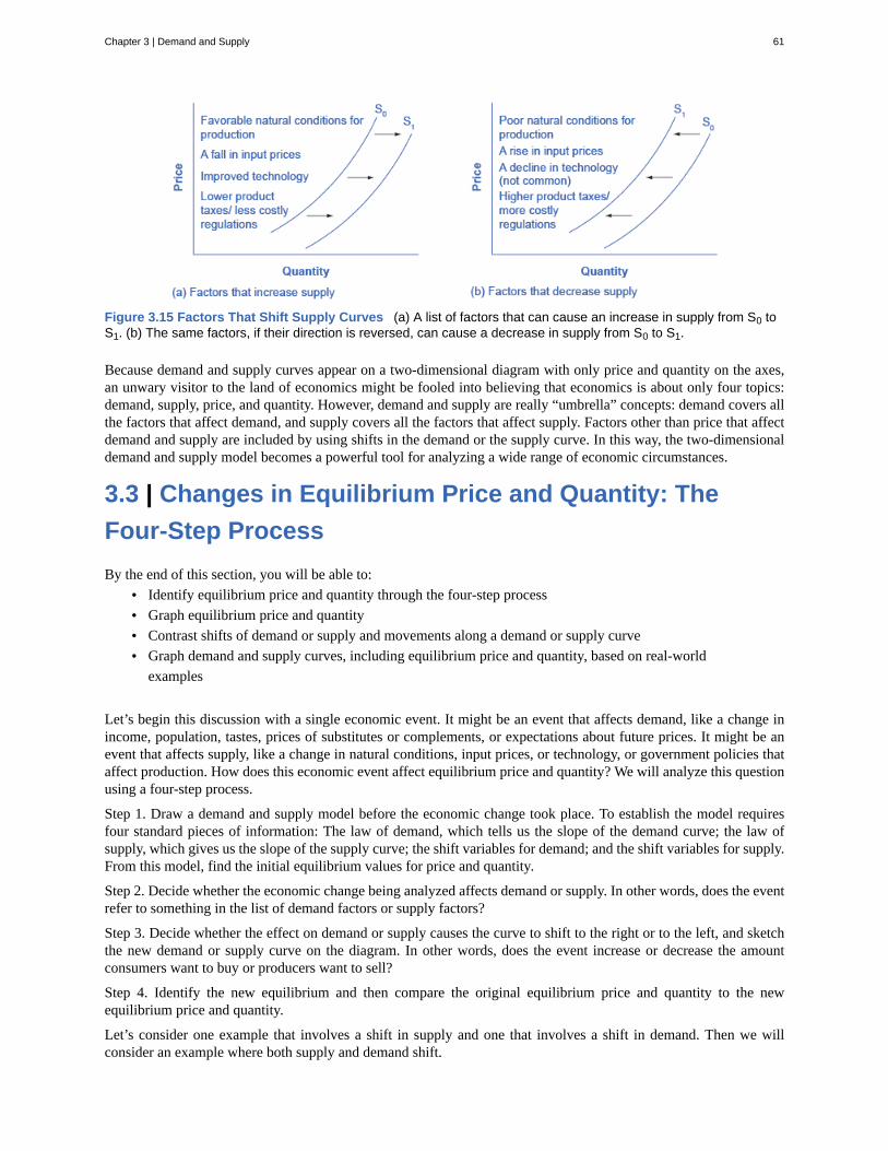
Figure 3.15 Factors That Shift Supply Curves (a) A list of factors that can cause an increase in supply from S0 toS1. (b) The same factors, if their direction is reversed, can cause a decrease in supply from S0 to S1.

Because demand and supply curves appear on a two-dimensional diagram with only price and quantity on the axes,an unwary visitor to the land of economics might be fooled into believing that economics is about only four topics:demand, supply, price, and quantity. However, demand and supply are really “umbrella” concepts: demand covers allthe factors that affect demand, and supply covers all the factors that affect supply. Factors other than price that affectdemand and supply are included by using shifts in the demand or the supply curve. In this way, the two-dimensionaldemand and supply model becomes a powerful tool for analyzing a wide range of economic circumstances.

3.3 | Changes in Equilibrium Price and Quantity: The

Four-Step Process

By the end of this section, you will be able to:• Identify equilibrium price and quantity through the four-step process• Graph equilibrium price and quantity• Contrast shifts of demand or supply and movements along a demand or supply curve• Graph demand and supply curves, including equilibrium price and quantity, based on real-world

examples

Let’s begin this discussion with a single economic event. It might be an event that affects demand, like a change inincome, population, tastes, prices of substitutes or complements, or expectations about future prices. It might be anevent that affects supply, like a change in natural conditions, input prices, or technology, or government policies thataffect production. How does this economic event affect equilibrium price and quantity? We will analyze this questionusing a four-step process.

Step 1. Draw a demand and supply model before the economic change took place. To establish the model requiresfour standard pieces of information: The law of demand, which tells us the slope of the demand curve; the law ofsupply, which gives us the slope of the supply curve; the shift variables for demand; and the shift variables for supply.From this model, find the initial equilibrium values for price and quantity.

Step 2. Decide whether the economic change being analyzed affects demand or supply. In other words, does the eventrefer to something in the list of demand factors or supply factors?

Step 3. Decide whether the effect on demand or supply causes the curve to shift to the right or to the left, and sketchthe new demand or supply curve on the diagram. In other words, does the event increase or decrease the amountconsumers want to buy or producers want to sell?

Step 4. Identify the new equilibrium and then compare the original equilibrium price and quantity to the newequilibrium price and quantity.

Let’s consider one example that involves a shift in supply and one that involves a shift in demand. Then we willconsider an example where both supply and demand shift.


3.1 | Demand, Supply, and Equilibrium in Markets for · When the price of gasoline rises, for example, it encourages profit-seeking firms to take several actions: ... Equilibrium—Where

Documents