3049269

THE UNIVERSITY OF ALBERTA

LATERALLY LOADED PILES

by

BRYNJA GUDMUNDSDOTTIR

A REPORT

SUBMITTED TO THE FACULTY OF GRADUATE STUDIES

I N PARTIAL FULFILMENT OF THE REQUIREMENTS FOR THE

DEGREE OF MASTER OF ENGINEERING

DEPARTMENT OF CIVIL ENGINEERING

EDMONTON, ALBERTA

FALL 198 1

UNIVERSITY OF ALBERTA

FACULTY OF GRADUATE STUDIES

The undersigned certify that they have read, and

recommend to the Faculty of Graduate Studies for acceptance,

a report entitled "Laterally Loaded Piles " as submitted by

Brynja Gudmundsdottir in partial fulfilment of the

requirements for the Degree of Master of Engineering.

Supervisor

Date

LATERALLY LOADED PILES

Submitted in partial fulfillment of the requirements

for the degree of Master of Engineering in

Geotechnical Engineering.

UNIVERSITY OF ALBERTA

Fall 1981 Brynja Gudmundsdottir

Table of Contents

Chapter Page

1 . INTRODUCTION ........................................... 1

2 . DESCRIPTION OF METHODS ................................. 3 2.1 Introduction ...................................... 3 2.2 Subgrade reaction method ........................... 4 2.3 Analytical design methods by subgrade reaction ..... 5 2.4 Broms' theoretical-empirical method ................ 8

2.4.1 Allowable lateral deflection at working loads ........................................ 8

2.4.2 Ultimate or failure load ..................... 9 2.4.3 Moments by Broms method ..................... 14

2.5 Matlock-Reese hand solution ....................... 16 2.5.1 Deflections ................................. 16

2.5.2 Moments ..................................... 20 2.6 Construction of p-y curves ........................ 20

2.6.1 Overconsolidated clay (Reese and Welch 1975) ....................................... 20

2.6.2 Normally consolidated clay (Matlock 1970) ... 21 2.6.3 Cohesionless soil (Reese. Cox and Koop ....................................... 1974) 23

2.7 Poulos method ..................................... 24 2.7.1 Elastic analysis ............................ 24 2.7.2 Calculation of displacement ................. 26 2.7.3 Calculation of moments ...................... 27

3 . CALCULATIONS .......................................... 41 ...................................... 3.1 Introduction 41

......... 3.2 Dimensions of pile and properties of soil 41

3.3 Broms method ...................................... 42 3.4 Calculation of p-y curves ......................... 42

3.4.1 Cohesive soil ............................... 43 3.4.2 Cohesionless soil ........................... 46

3.5 Matlock-Reese hand solution ....................... 52 3.5.1 Deflections ................................. 52

..................................... 3.5.2 Moments 52

3.6 Poulos method ..................................... 61 3.7 Summary of results ................................ 62

4 . DISCUSSION OF RESULTS ................................. 63 4.1 Introduction ...................................... 63 4.2 Cohesionless soil ................................. 63 4.3 Cohesive soil ..................................... 64

References ............................................... 68

L i s t of Tables

Table Page

2.1 Evaluation of the coefficient n. and n. ............ 39 2.2 Coefficient of horizontal subgrade

reaction k for cohesionless soil .................. 39 2.3 Coefficient and equations for ............................... Matlock-Reese method 40

.................... 3.1 Soil parameters used in example 42

3.2 Calculation of y and M by Broms method ............. 43 3.3 Calculation of p-y curve for .............................. overconsolidated soil 44

3.4 Calculation of p-y curve for normally .................................. consolidated soil 47

3.5 Coefficient A and B for calculation of ultimate resistance for cohesionless soil .......... 49

3.6 Calculation of p-y curve for cohesionless ............................................... soil 50

3.7 Calculation of y by Matlock-Reese method . Overconsolidated clay .............................. 53

3.8 Calcualtion of y by Maltoc-Reese method . Normally consolidated clay ......................... 54

3.9 Calcualtion of y by Matlock-Reese method . .................................. Cohesionless soil 56

3.10 Calculation of y and M by Poulos method ............ 61 3.11 Summary of results using different methods ......... 62

i i i

List of Figures

Figure Page

2.1 Distribution of lateral pressure in soil ........... 28 ..................... 2.2 Beam column under lateral load 28

2.3 Cohesive soil . Lateral deflection at ..................................... ground surface 29

2.4 Cohesionless soil . Lateral deflection at ..................................... ground surface 29

2.5 Cohesive soil . Ultimate lateral ......................................... resistance 30

2.6 Cohesionless soil . Ultimate lateral .

resistance ......................................... 31 .................. 2.7 Graphical definition of p-y curve 32

................. 2.8 Typical reaction-deflection curves 32

................. 2.9 Trial plots of soil modulus values 33

............... 2.10 Interpolation for stiffness factor T 33

2.71 Characteristic shapes of p-y curve for .......................................... soft clay 34

2.12 Typical family of p-y curves in cohesionless soil .................................. 34

2.13 Non-dimensional coefficients for ultimate soil resistance vs depth in sand ................... 35

2.14 Influence factor I ................................. 35 .......................... 2.15 Influence factor I and I 36

................................. 2.16 Influence factor I 36

2.17 Influence factor I ................................. 37 2.18 Maximum moment in free-head pile ................... 37 2.19 Fixing moment at head of fixed-head pile ........... 38 3.1 Example calculated ................................. 41 3.2 P-y curves for overconsolidated clay ............... 45

.......... 3.3 P-y curves for normally consolidated soil 48

Figure Page

.................... 3.4 P-y curve for cohesionless soil 51

3.5 Interpolation for final value of relative .......................................... stiffness 57

3.6 Trial plots of soil modulus values - Overconsolidated clay .............................. 58

3.7 Trial plot of soil modulus values - Normally consolidated clay ......................... 59

3.8 Trial plot of soil modulus values - .................................. Cohesionless soil 60

NOTAT I ON

Symbol Unit

A - - Definition

Coefficient for ultimate soil resistance

(p-y curve :sand)

Coefficient for moment (Matlock-Reese)

Coefficient for slope (Matlock-Reese)

Coefficient for deflection due to shear

(Matlock-Reese)

Coefficient for soil resistance (p-y

curve:sand)

Coefficient for moment (Matlock-Reese)

Coefficient for slope (Matlock-Reese)

Coefficient for deflection due to moment

(Matlock-Reese)

Coefficient in the parabolic section (p-y

Undrained shear strength

Shape factors for steel piles (Broms)

Coefficient for deflection (Matlock-Reese)

Diameter or width of pile

Modulus of elasticity - Youngs modulus Modulus of elasticity of pile

Soil modulus (Matlock-Reese)

Eccentricity of load

Distance from ground surface or 1.5 pile

diameter below ground surface to location

of maximum bending moment (Broms)

Yield stress of pile material (Broms)

Moment of inertia

Moment of inertia of pile section

Displacement influence factor for applied

horizontal load (Poulos)

Displacement influence factor for applied

moment(Pou1os)

Displacement influence factor for fixed

head pile (Poulos)

Rotation influence factor for applied

horizontal load (Poulos)

Rotation influence factor for applied

moment (Poulos)

Empirical adjustment factor (p-y curve

soft clay)

Coefficient fo earth pressure

Coefficient of active earth pressure

Coefficient of earth pressure at rest

Coefficient of passive earth pressure

Pile flexibility factor

Coefficient of horizontal subgrade

reaction

Coefficient of soil modulus (Matlock

-Reese )

Embedded length of pile

Moment

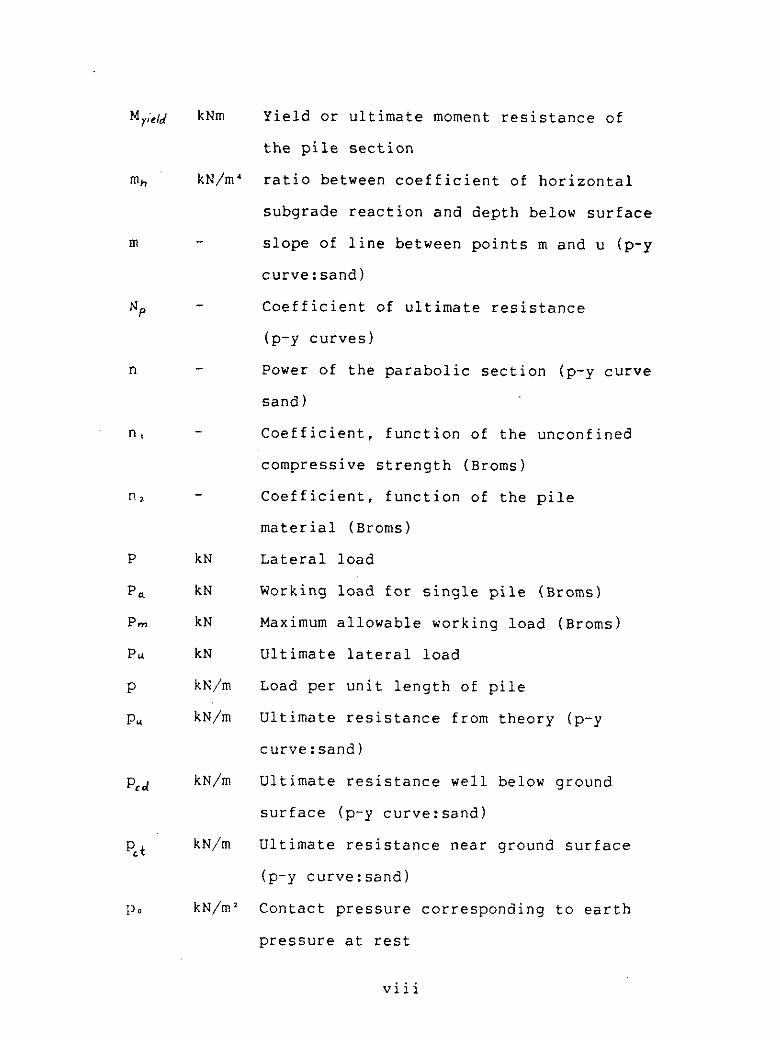
Yield or ultimate moment resistance of

the pile section

ratio between coefficient of horizontal

subgrade reaction and depth below surface

slope of line between points m and u (p-y

curve:sand)

Coefficient of ultimate resistance

(p-y curves)

Power of the parabolic section (p-y curve

sand)

Coefficient, function of the unconfined

compressive strength (Broms)

Coefficient, function of the pile

material (Broms)

Lateral load

Working load for single pile (Broms)

Maximum allowable working load (Broms)

Ultimate lateral load

Load per unit length of pile

Ultimate resistance from theory (p-y

curve:sand)

Ultimate resistance well below ground

surface (p-y curve:sand)

Ultimate resistance near ground surface

(p-y curve:sand)

Contact pressure corresponding to earth

pressure at rest

J'm m

il: m

Contact pressure on vertical face for

horizontal displacement y o

Contact pressure on area acted upon by

active earth pressure

Contact pressure on area acted upon by

passive earth pressure ( = pi + p)

Axial load

Unconfined compressive strength

Slope of the pile

Section modulus about an axis perpendicular

to the load plane

Relative stiffness factor (Matlock-Reese)

Shear force

Depth below ground surface

Depth below ground surface to transition

in coefficient of ultimate resistance

equation (p-y curve:soft clay)

Depth below ground surface to transition

in ultimate soil resistance equation (p-y

curve: sand)

Displacement of pile

Initial displacement, required for

increasing the coefficient of earth

pressure on a vertical wall from K O to K.

Deflection at point m (p-y curve: sand)

Deflection of point k (p-y curve: sand)

Deflection at one half the ultimate soil

resistance

Depth coefficient (Matlock-Reese)

Unit weight of the soil

Poisson's ratio

Factor for cohesive soil (Broms)

Factor for cohesionless soil (Broms)

Dimensionless length factor for

cohesive soil

Dimensionless length factor for cohesion-

less soil

Strain corresponding to one ha.lf the

maximum principal stress difference

Angle of internal friction

Overburden pressure.

Pile rotation

1. INTRODUCTION

Large lateral loads and moments on superstructures

caused by waves, winds, seismic forces, surcharges etc. are

transferred to the desired soil strata by means of a single

pile or a pile group.

In designing piles for lateral load, the designer

should avail himself of more than one method whenever

possible.

In this project a single active pile will be

investigated. The deflection at the ground surface and the

maximum moment in the pile will be calculated. This will be

done for three different methods and the results will be

compared for different types of cohesive soil

(overconsolidated clay and normally consolidated clay), and

for cohesionless soil (medium dense sand). However

comparison with test result for calculated values is not

possible because the examples are calculated by taking

representative values for the properties of each type of

soil . Many different methods for calculating the lateral

capacity of piles are presented in the literature. Those

selected here are the ones developed by Broms (1964a) and

(1964b), Matlock-Reese (1961) and Poulos (1971). All these

methods are well known and are widely used.

In chapter two the methods are introduced and

described. The theory on which they are based is reviewed,

togerther with how the parameters are used in each method.

In chapter three the example design problem is

introd,uced and used are given. The deflection at the ground

surface and the maximum moment in the pile are calculated

for these methods.

In chapter four the results are discussed and compared

and explanation is sought when they do not agree.

2. DESCRIPTION OF METHODS

2.1 Introduction

In this chapter the methods used are reviewed. First

the subgrade reaction coefficient is explained, based mainly

on the work of Terzaghi (1955) and McClelland and Focht

(1958). The differential equation which the subgrade

reaction method has as its basis is presented, togerther

with how it is used for both the Broms method and the

Matlock-Reese method.

Broms (1964a and b) method is outlined both for

cot.esive and cohesionless soil. The Matlock-Reese (1961)

hacd solution is reviewed, and also the construction of p-y

(soil reaction-pile deflection) curves which is necessary to

use that method. Construction of p-y curves is based on

Recse et.a1.(1975) for overconsolidated clay or stiff clay,

on Matlock (1970) for normally consolidated clay or soft

clay, and on Reese et.al. (1974) for cohesionless soil. The

last method that is reviewed is the one by Poulos (1971)

which is based on an elastic solution. The elastic analysis

is discussed, followed by a description of how calculation

is done by this method.

2.2 Subgrade reaction method

The coeffient of horizontal subgrade reaction k, is

defined as the ratio between a horizontal pressure per unit

area of vertical surface and the corresponding horizontal

displacement. Thus it is a measurement of the ability of the

soil to resist horizontal deformation. The value of k,

depends on the elastic properties of the subgrade and on the

dimension of the area acted upon by the subgrade pressure.

Consider a pile which has been driven into or is buried

in subgrade. Before any horizontal force has been applied to

the pile, the surface of contact between the pile and the

subgrade is acted upon at any depth x below the surface by a

pressure p. which is equal to or greater than the earth

pressure at rest. If the pile is moved to the right the

pressure at the left side will drop to very small value and

on the right side will increase from p, to pb. The lateral

displacement y, required to produce this change is very

small and can be neglected. After the pile has moved a

distance y , the pressure at each side will be:

left side (active state) p = O (2.1)

right side (passive state) p =pb+k,y, (2.2)

The subgrade modulus of a stiff clay, k h , is generally

considered to have the same value at every point of the

subgrade contact, independent of depth. Therefore, at any

time, the subgrade reaction p is almost uniformly

distributed over the right hand face of the pile. However,

due to progressive consolidation of clay under constant

load, y, increases and k decreases with time. Both

quantities approach an ultimate value, which is the value

that Should be used in design.

For cohesionless subgrade material the values of k,, and

y, are independent of time. However, the elastic modulus of

sand increases with depth, therefore the coefficient of

subgrade reaction is determined by kh=mhx where x is the

depth below subgrade and m is the ratio between coefficient

of horizontal subgrade reaction and depth below surface. The

value mh is assumed to be the same for every point of the

surface contact (Figure 2 .1 ) .

The width D of the pile also influences the horizontal

displacement. For piles of diameter D, and nD, the lengths

of the bulbs of pressure measured in the direction of

movement of the pile are L and nL respectively (see Figure

2 . 1 ) Furthermore in both clay and sand the modulus of

elasticity is constant in the horizontal direction. Hence in

clay as well as in sand the horizontal displacement y '

increases in direct proportion to the width D.

2.3 Analytical design methods by subgrade reaction

For solving laterally loaded piles the pile-soil system

is treated as analogous to a beam on an elastic foundation.

These analyses have as their basis the Winkler model, which

assumes that a medium can be approximated by an infinite

series of closely-spaced, independent springs.

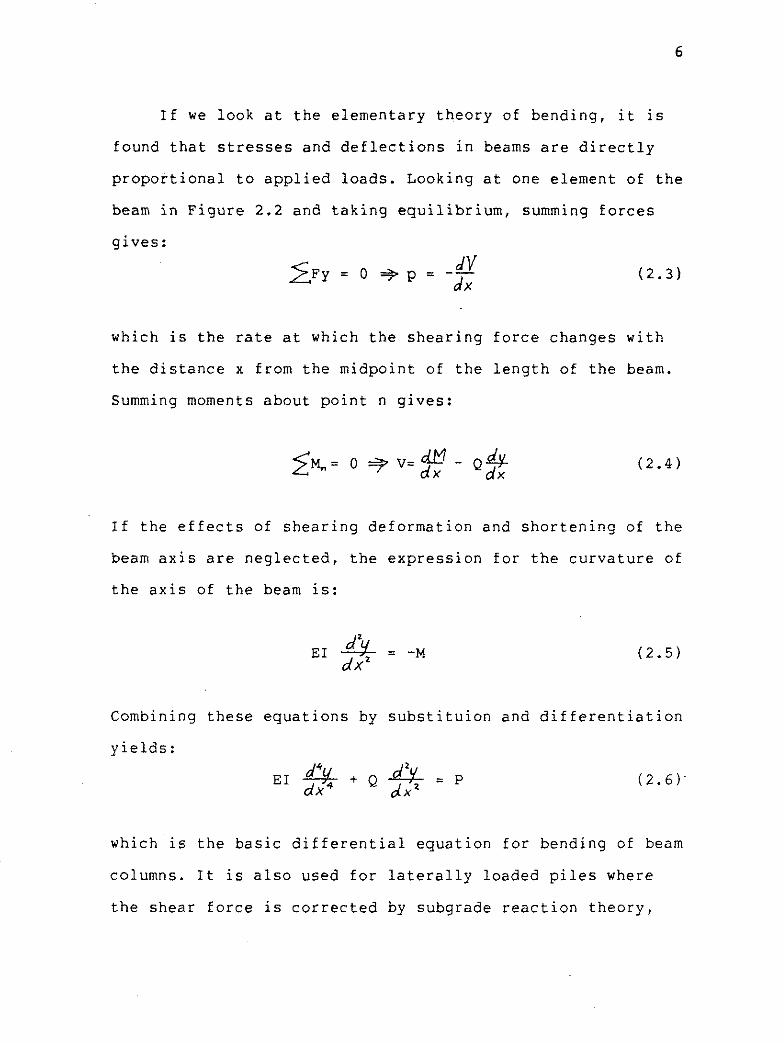
If we look at the elementary theory of bending, it is

found that stresses and deflections in beams are directly

proportional to applied loads. Looking at one element of the

beam in Figure 2.2 and taking equilibrium, summing forces

gives:

which is the rate at which the shearing force changes with

the distance x from the midpoint of the length of the beam.

Summing moments about point n gives:

If the effects of shearing deformation and shortening of the

beam axis are neglected, the expression for the curvature of

the axis of the beam is:

dZ EI Y = -M dx'

Combining these equations by substituion and differentiation

yields:

which is the basic differential equation for bending of beam

columns. It is also used for laterally loaded piles where

the shear force is corrected by subgrade reaction theory,

and y increases approximately in proportion to the applied

load.

For cohesive soil the shear force is the horizontal

pressure and is equal to:

For cohesionless soil it becomes:

bkcause modulus of elasticity increases approximately in

direct proportion to depth. Therefore it is assumed without

serious error that the pressure p required to produce a

given horizontal displacement y increases in direct

proportion to the depth as shown. Equation 2.6 then becomes:

To solve this equation one must make assumptions concerning

the end conditions and then determine the constants.

Both Broms and Matlock-Reese use this equation for

their solution. Broms assumes that the axial load is

negligible compared to the buckling load, and he uses the

shear force as previously described. Matlock-Reese use an

iterative procedure to account for the non-linear behaviour

relationship between pile deflection and soil resistance,

until satisfactory compatibility is obtained between the

predicted behaviour of the soil and the load-deflection

relationship required by an elastic pile.

2.4 Broms' theoretical-empirical method

For the coefficient of horizontal subgrade reaction,

Broms uses Terzaghi's values for cohesionless soils. For

cohesive soil he established the following expression:

The use of 80q, gives good agreement with Terzaghi's values

The value n, is a function of the unconfined compressive

strength q,,n, is a function of the pile material, and D is

the pile diameter. The values of n, and n, are given in

Table 2.1. The values of k, for cohesionless soil are given

in Table 2.2 for both Terzaghi's and Reese's

recommendations.

For design Broms developed two basic design conditions,

which are discussed below.

2.4.1 Allowable lateral deflection at working loads

Broms made the simplifying assumption that the axial

load is negligible compared to the buckling load, and

equation (2.6) thus reduces to

He solved this 'equation for three pile conditions:

1 ) Fixity: free-headed or restrained,

2 ) Length: short, intermediate or long,

3 ) Soil type: cohesive or cohesionless.

He incorporated the criteria for various pile conditions in

the corresponding equations and developed graphical

relationships. From these curves it is possible to determine

either the theoretical lateral deflection or the theoretical

applied load if the other is known. Allowable lateral

deflection or allowable load can then be determined by

applying the appropriate adjustments.

2.4.2 Ultimate or failure load

This criterion assumes two modes of failure:

1 ) shear in the soil in the case of short stiff piles,

2 ) bending of the pile in the case of long piles (as

governed by the plastic yield resistance of the pile

section).

In the case of long piles Broms assumed that the pile

developed plastic hinges permitting sufficient rotation to

mobilize the bending moments along the pile length. Based on

these assumptions he treated the pile as a statically

determinant beam with a distributed load corresponding to

the particular condition. Below is a summary of the design

procedure for Broms' method. Figures that are referred to

are at the end of the chapter.

Summary of Broms design method.

STEP 1:

Determine the general soil type (cohesive or cohesionless)

within the critical depth below the surface (about four to

five pile diameters D)

STEP 2:

Determine the horizontal coefficient of subgrade reaction k

within the critical depth from equation (2.8) for cohesive

soil, or by selecting an appropriate value from Table 2.2

for cohesionless soil.

STEP 3:

Adjust kh for loading and soil conditions:

a. Cyclic loading in cohesionless soil:

1. k,= 1/2k, from Step 2 for medium to dense sand

2. k,= 1/4k, from Step 2 for loose soil

b. Static loads resulting in soil creep:

1. Soft and very soft normally consolidated clays

k,= (1/3 to 1/6) k, from Step 2

2. Stiff to very clays

kh= ( 1 / 4 to 1/2) kh from Step 2

STEP 4:

Determine pile parameters:

a. Modulus of elasticity E

b. Moment of inertia I

c. Section modulus S about an axis perpendicular to the load

plane

d. Yield stress of pile material fy

e. Embedded pile length L

f. Diameter or width D

g. Eccentricity of applied load e for free-headed piles

- - i.e., vertival distance between ground surface and

lateral load

h. Dimensionless shape factor C, (for steel piles only):

1. Use 1.3 for piles with circular cross-section

2. Use 1.1 for H-section when the applied load is in the

direction of the pile's maximum resisting moment

(normal to pile flanges).

3. Use 1.5 for H-section piles when the applied load is

in the direction of the pile's minimum resisting

moment (parallel to pile flanges)

i. M , the resisting moment of the pile = C,f,S

STEP 5:

Determine factor B or 1:

a. B = d m for cohesive soil, or

b. 9 = d z for cohesionless soil

STEP 6:

Determine the dimensionless length factor:

a. BL for cohesive soil, or

b. qL for cohesionless soil.

STEP 7:

Determine if the pile is long or short:

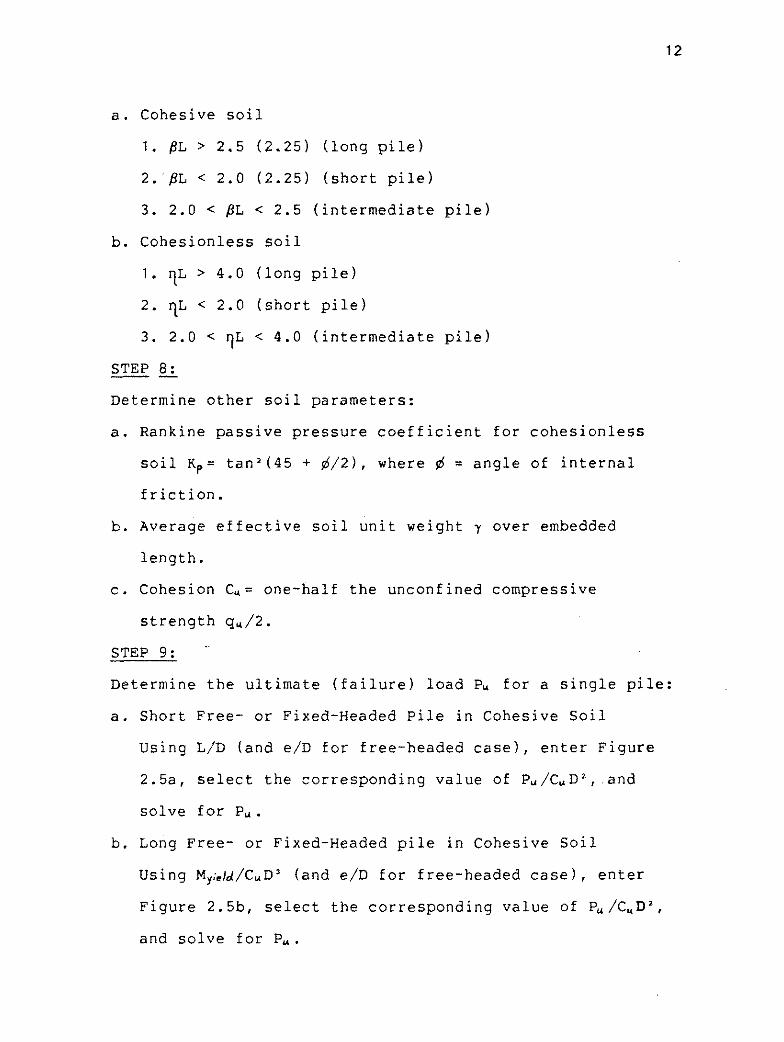
a. Cohesive soil

1. ,!3L > 2.5 (2.25) (long pile)

2. flL < 2.0 (2.25) (short pile)

3. 2.0 < ,!3L < 2.5 (intermediate pile)

b. Cohesionless soil

1. YL > 4.0 (long pile)

2. qL < 2.0 (short pile)

3. 2.0 < qL < 4.0 (intermediate pile)

STEP 8: -- Determine other soil parameters:

a. Rankine passive pressure coefficient for cohesionless

soil Kp= tan2(45 + 6/2), where 6 = angle of internal

friction.

b. Average effective soil unit weight y over embedded

length.

c. Cohesion Cu= one-half the unconfined compressive

strength q,/2.

STEP 9:

Determine the ultimate (failure) load P, for a single pile:

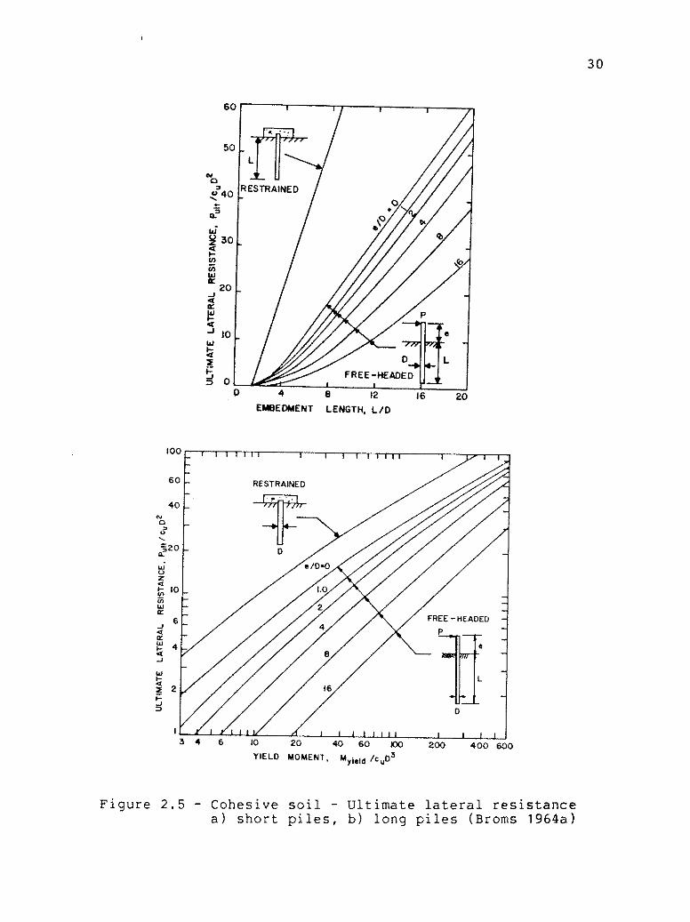
a. Short Free- or Fixed-Headed Pile in Cohesive Soil

Using L/D (and e/D for free-headed case), enter Figure

2.5a, select the corresponding value of PU/C,D2, and

solve for P, . b. Long Free- or Fixed-Headed pile in Cohesive Soil

Using My;.ld/CuD3 (and e/D for free-headed case), enter

Figure 2.5b, select the corresponding value of Pu/C,D2,

and solve for P, .

c. Short Free- or Fixed-Headed Pile in Cohesionless Soil

Using L/D (and e/L for the free-headed case), enter

Figure 2.6a, select the corresponding value of Pu/ KpD3y,

and solve for P, . d. Long Free- or Fixed-Headed Pile in Cohesionless Soil

Using Myield/D'yKp, (and e/D for the free-headed case),

enter Figure 2.6b select the corresponding value of P,/ Kp

D3y, and solve for Pa.

e. Intermediate Free- or Fixed-Headed Pile in Cohesionless

Soil

Calculate P for both a short pile (Step 9c) and a long

pile (Step 9d) and use smaller value.

STEP 10:

Calculate the maximum allowable working load for a single

pile P, from the ultimate load P, determined in Step 9:

P,= Pu/2.5

STEP 1 1 :

Calculate the working load for a single pile Pa

corresponding to a given design deflection y at the ground

surface, or the deflection corresponding to a given design

load. If P, a n d y are not given, substitute the value of Pm

from Step 10 for Pa in the following cases and solve for y,:

a. Free- or Fixed-Headed Pile in Cohesive Soil

Using pL (and e/L for the free-headed case),enter Figure

2.3, selecting the corresponding value of ykhDL/P,, and

solve for Pa or y.

b. Free- of Fixed-Headed Pile in Cohesionless Soil

Using nL (and e/L for the free-headed case), enter Figure

2.4, select the corresponding value of y (EI ) d5k'fS/pa L,

and solve for Pa or y.

STEP 12:

If Pa> P,, use P, and calculate y, (Step 1 1 )

If Pa < P,, use Pa and y.

If Pa and y are not given,use P, and y,.

STEP 13:

Reduce the allowable load selected in Step 12 to account for

method of installation: for driven piles use no reduction,

and for jetted piles use 0.75 of the value.

2.4.3 Moments by Broms method

The mode of failure of laterally loaded pile depends on

the depth of embedment and on the degree of end restraint.

For short piles failure takes place when the soil

yields along the total length of the pile, and the pile

rotates as a unit around a point located at some depth below

ground surface (in the case of a free head pile) Restrained

failure takes place when the applied load Is equal to the

ultimate lateral resistance of the soil, and the pile moves

as a unit through the soil.

For long piles the mechanism of failure is when a

plastic hinge forms at the location of the maximum bending

moment. Failure takes place when the bending moment is equal

to the moment resistance of the pile section (for free-head

piles). Restrained pile failure takes place when two plastic

hinges form along the pile. The two plastic hinges form when

the maximum positive bending moment at depth f or (1.5D + f)

below ground surface, and the maximum negative bending

moment at the bottom of the pile cap or lateral bracing

system, both reach the yield resistance of the pile section.

For the case of a restrained pile, an intermediate

length of pile has also to be taken into account. In this

case failure takes place when the restraining moment at the

head of the pile is equal to the ultimate moment resistance

of the pile section, and the pile rotates around a point

located at some depth below the ground surface.

The maximum moment occurs at the depth below surface

where the shear force in the pile is equal to zero, at depth

(f + 1.5D) for cohesive soil and f for cohesionless soil.

Cohesive soil:

The distance f and the maximum bending moment M,,, can

be calculated from the two equations

P f = - and = P(e + 1.5D + 0.5f) (2.9) 9Cu D M,,,

Cohesionless soil:

Here it has been assumed that lateral deflections are

sufficiently large at failure to develop the full passive

resistance (equal to three times the passive Rankine earth

pressure), from the ground surface to the location of

maximum bending moment. Thus we have for free-head piles:

£ = 0 . 8 2 J m and ME= P(e + 0.67f) + Qa (2.10)

2.5 Matlock-Reese hand solution

2.5.1 Deflections

When using this method a set of p-y curves are needed.

Here they will be constructed semi-empirically for a static

loading condition and will be described in next section.

The primary solution will consist of finding the set of

elastic deflections of the pile (including the short jacket

leg extension) which will simultaneously satisfy:

1 ) the non-linear resistrance deformation relations

which are predicted for the soil,

2) the elastic bending properties of the piles,

3) the angular stiffness of the upper structure at the

pile to structure connection.

The force-deformation characteristics of the soil are

described by a set of predicted p-y curves. In Figure 2.7

there is a graphical definition of p-y curves and in Figure

2.6 there are typical resistance curves for soil at various

depths. Since solution for the interaction problem relies on

repeated applications of elastic theory, a secant modulus of

qrril reaction E, is required, which is defined as E, = -p/y.

This is only a computation device which is generally

independent of pile size and depends primarily on soil

properties (not a unique soil property).

The differential equation for a beam is:

This is the same equation as used for Broms' method. Here

this equation is solved by trial and error by estimating the

value of T, relative stiffness factor, until T&fa;m/is equal

to Ttried. Then correct set of E, are found and deflection

and bending moments are computed.

In this solution the deflection y of the pile at any

depth x is:

where A T , By are functions of z = x/T, relative stiffness

factor T is T 5 = EI/k, and subscript t refers to the pile at

the top.

It is convenient to define an additional set of

nondimensional deflection coefficients by rearranging

equation (2.11) as:

Pt T3 y = Cy- w i

E I where C,,= A y + -

P, T (2.12)

To begin the solution of the example problem it is necessary

to assume temporarily that the form of soil modulus

variation E,= kx will be a satisfactory approximation of the

actual final E, variation. Available non-dimensional

solutions are limited to a pile of constant bending

stiffness.

The slope at the top of the pile is:

where subscript s stands for shear and subscript t for at

top.

The relation between Mt and St is:

Combining these two equations yields:

M A s t T 2 = - P" ~ - B ~ ~ T

3.5

Since the relative stiffness factor T depends on the

coefficient of soil modulus variation k and this quantity in

turn depends on non-linear resistance characteristics, the

solution must proceed by a repeated trial and adjustments of

the values of T (or k ) until the deflection and resistance

patterns of the pile agree as closely as possible with the

resistance-deflection (p-y) relations previously estimated

for the soil. Even though the final set of secant modulii (E,

= - p/y) may not vary in a perfectly linear fashion with

depth, proper fitting of E,= kx will usually produce

satisfactory solutions.

The steps in the Matlock-Reese method are as follows:

Calculations are made for certain depths x

Estimate the first value of T (trial value)

Calculate z = x/T

Find the coefficients A y and B5, given in Table 2.3

(or find Cy)

Calculate y from equation (2.11)

Find p for this y from p-y curves

Calculate E, = -p/y

Set up a graph E, vs x and find k from this graph

(see Figure 2.9), and giving more weight to points at

depth less than x = 0.5T.

9) Calculate T . ~ f ~ ; ~ ~ d = '

10) Compare T~f~;"~dand Tt,;,/ and when they are the same

the trial and error process is completed. Use a

graph of T,,, vs T,bf,;& (see Figure 2.10. ) The final

set of computations for the E value is made as a

check.

2 . 5 . 2 Moments

Computations of values of bending moments along the

pile are made by application of the equation:

The non-dimensional coefficients A and B are found in

Table 2.2. Subscript m refers to moments.

2 . 6 Construction o f p-y curves.

2 . 6 . 1 Overconsolidated clay (Reese and Welch 1975)

The step by step procedure for this material is:

1 ) Obtain the best possible estimate of the variation

of shear strength and effective unit weight with depth,

and of the value of E , , , the strain corresponding to

one-half the maximum principal stress difference. If no

value of &,, is available use a value of 0.005 or 0.010,

the larger value being more conservative. Here the lower

value will be used, I?,,= 0.005 (Reese and Welch).

2 ) The ultimate soil resistance p is computed according to:

and the smaller value is used for each depth.

3 ) Compute displacement y,, at one-half the ultimate soil

resistance.

y,. = 2.5D6,,

4) The points on the curve are now computed by:

(Beyond y = 16y,,, p = p, for all values of y )

2.6.2 Normally consolidated clay (Matlock 1970)

The steps are the same as for overconsolitated clay but

the values and equations are different. The procedure given

here is for submerged clay soils, which are normally

consolidated or slightly overconsolidated.

1 ) Here the value of e , , may be assumed to be between 0.005

and 0.020, the smaller value being more applicable to

brittle or sensitive clay and the larger value to

disturbed or remolded soils or unconsolidated sediments.

An intermediate value of E , , = 0.010 is probably

satisfactory for most purposes.

2) Ultimate resistance.

If soft clay soil is confined so that plastic flow

around a pile occurs in horizontal planes, the ultimate

resistance per unit length of pile may be expressed as:

p, = N,, G D (2.20)

where

9 at a considerable depth below the surface x

N = 3 + + J - (between the free soil surface L'4 0

and depth the variation is

described by this equation)

2-4 very near the surface in front of the pile

3 (for a cylindrical pile, this is believed to 1 be appropriate)

The value of J should to be determined empirically.

Here the value of J = 0.5 will be used as it is

considered to be appropriate for this type of clay.

3 ) Compute y,, using Skempton's approach

4 ) The points on the curve are now computed by

Beyond y = 8y,,, p = p, for all values of y. The final

shape of the p-y curve of clay is shown in Figure 2.11

for normally consolidated clay. The shape for

overconsolidated clay is almost the same but the power in

the equation is different.

2.6.3 Cohesionless soil (Reese, Cox and Koop 1974)

For construction of p-y curves for sand, the outline

from Reese et.a1.(1974) is used. The method is based on

theory as well as empiricism.

Recommended procedure:

1) Obtain soil properties and pile dimensions 6 , y , D

2 ) Use the following parameters for computing soil

resistance:

d a = - 4 0 , f l = 45 + T , K, = 0.4, Ka= tan1(45-7)

3 ) The following equation are used to calculate soil

resistance:

a ) Ultima~te resistance near ground surface:

KO H tan@s;np + f a n P PC+= YH( tan$-4)ro# (D+HtanBtana) + taofp-b)

b) Ultimate resistance well below the ground surface.

gd= KaDyH(tan8fi-1) + K,DyHtan$tan'B (2.24)

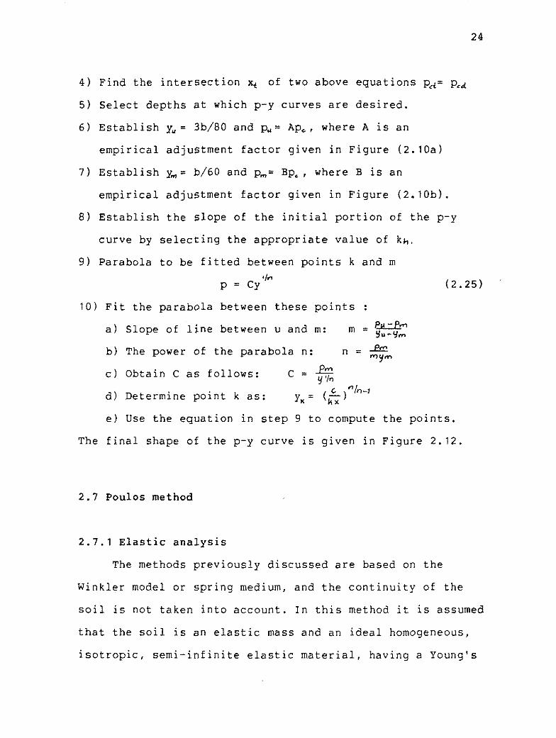
4) Find the intersection xt of two above equations pd= pcd

5) Select depths at which p-y curves are desired.

6 ) Establish y, = 3b/80 and p, = Ap, , where A is an

empirical adjustment factor given in Figure (2.10a)

7) Establish y, = b/60 and p,= Bp, , where B is an

empirical adjustment factor given in Figure (2.10b).

8 ) Establish the slope of the initial portion of the p-y

curve by selecting the appropriate value of kh.

9) Parabola to be fitted between points k and m

p = cy'ln

10) Fit the parabola between these points :

a) Slope of line between u and m: m = P d m Yu-Yrn

b) The power of the parabola n: n = 9rr "Y"

C) Obtain C as follows: C = fk y % c n/n-l d) Determine point k as: Y,= (k7;)

e) Use the equation in step 9 to compute the points.

The final shape of the p-y curve is given in Figure 2.12

2.7 Poulos method

2.7.1 Elastic analysis

The methods previously discussed are based on the

Winkler model or spring medium, and the continuity of the

soil is not taken into account. In this method it is assumed

that the soil is an elastic mass and an ideal homogeneous,

isotropic, semi-infinite elastic material, having a Young's

modulus E and Poisson's ratio y, which are unaffected by

the presence of the pile.

In this analysis the pile is assumed to be a thin

rectangular strip of width D ( or if circular the diameter

is used instead of the width), length L and having constant

flexibility EXp.

For an elastic condition the horizontal shear stress

developed between the soil and the sides of the pile is not

taken into account. The pile is divided into elements all of

equal length except the top and bottom elements which are of

half length. Each element is acted upon by a uniform

horizontal stress p which is assumed to be constant across

the width of the pile.

For this condition the horizontal displacement of the

soil and of the pile are equal along the pile (for purely

elastic conditions). In this analysis the soil and pile

displacements are evaluated and equated at the element

center, except for the top and bottom elements where

displacements are calculated by equating soil and pile

displacements at these points. Using the appropriate

equilibrium conditions, sufficient equations are qbtained to

solve for the unknown horizontal displacement at each

element.

Two conditions of practical interest at the pile head

are considered:

1 ) a free-head pile, free rotation occurs

2 ) a fixed-head pile, no rotation occurs

Two major variables influencing pile behaviour are the

length to diameter ratio L/D and a factor K R , herein known

E I as the pile flexibility factor K R = *, a dimensionless E L

measure of the flexibility of the pile relative to the soil.

2.7.2 Calculation of displacement

Calculations by this method are performed by using

charts. Displacement and rotation are expressed in terms of

dimensionless influence factors which are function of the

pile flexibility factor K . The length to diameter ratio is relatively small so y,= 0.5 may be used for all conditions.

The horizontal displacement is expressed as:

for a f ree-head pile P rvl Y = +fJT + I -

YM EL

for a f ixed-head pile P y = I - YF E L

The rotation 8 for a free-head pile is:

Values of Iy,, are given in Figures 2 . 1 4 to 2 . 1 7 . From theory

IyM and I,M should be the same but this is not quite true.

The difference is usually 5% except for very flexible piles

where it is 10 to 1 5 % . This discrepancy indicates the order

of accuracy of the corresponding values of Is,.

2.7.3 Calculation of moments

Moments are calculated by charts of K and L/D. From

these charts the value M/PL is obtained from Figure 2.18 for

free-head piles and Figure 2.19 for fixed-head piles. For

free-head piles the maximum moment is at depth of 0.1L to

0.4L below the surface, the lower value being associated

with stiffer piles. For fixed-head piles the maximum moment

is at the head of the pile except if the pile is very

flexible.

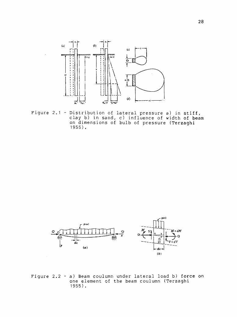
Figure 2.1 - Distribution of lateral pressure a) in stiff, clay b) in sand, c ) influence of width of beam on dimensions of bulb of pressure (Terzaghi 1955).

Figure 2.2 - a ) Beam coulumn under lateral load b) force on one element of the beam coulumn (Terzaghi 1955).

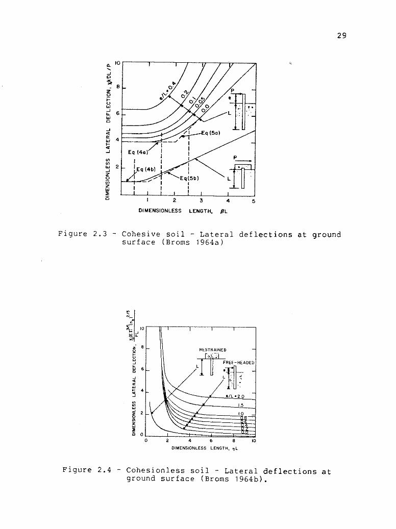
DIMENSIONLESS LENGTH. BL

Figure 2.3 - Cohesive soil - Lateral deflections at ground surface (Broms 1964a)

i 8 g RESTRAINED

0 Y J ,L

X 6 J 4 u g 4

", Y g 2

W E 0 0

OIMENSIONLESS LENGTH, 11

Figure 2.4 - Cohesionless soil - Lateral deflections at ground surface (Broms 1964b).

E W E W E N T LENGTH. L I D

YIELD MOMENT. Mpleld /c,,03

Figure 2.5 - Cohesive soil - Ultimate lateral resistance a) short piles, b ) long piles (Broms 1964a)

Figure 2.6 - Cohesionless soil - Ultimate lateral resistance a ) short piles, b) long piles (Broms 1964b)

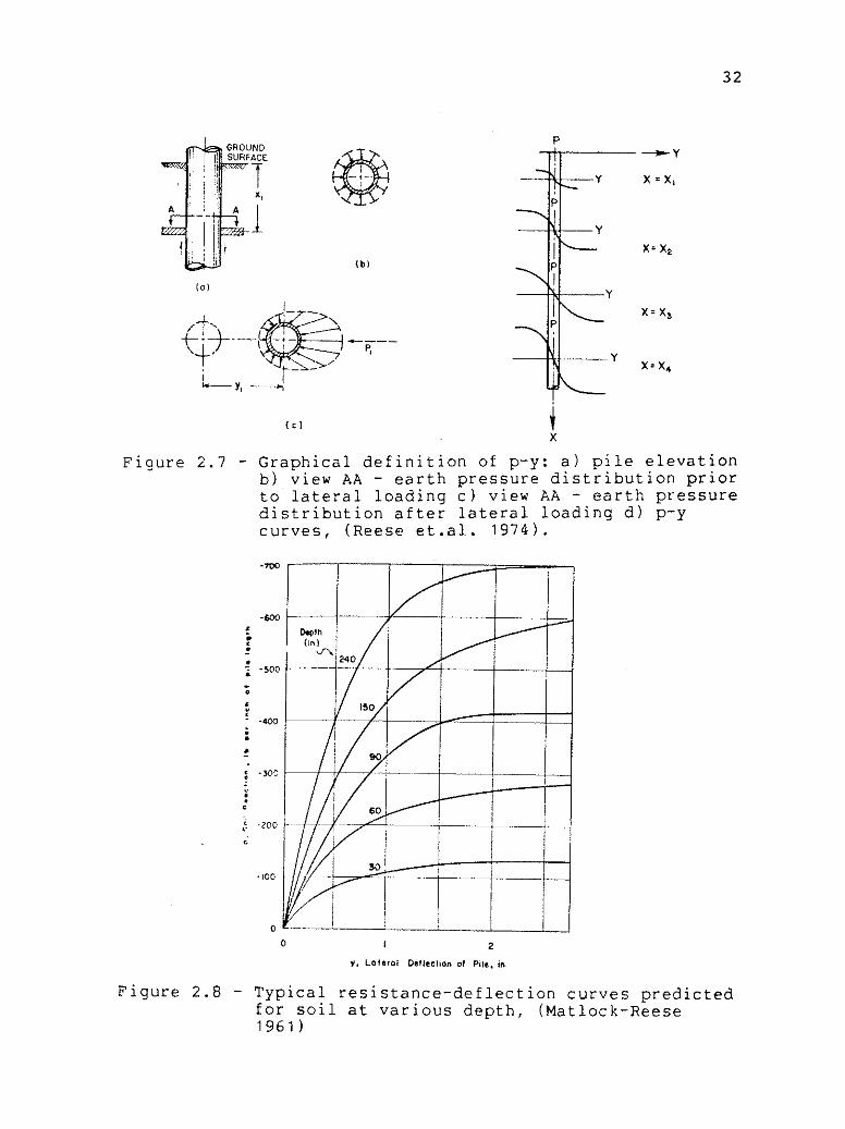
Figure 2.7 - Graphical definition of p-y: a) pile elevation b) view AA - earth pressure distribution prior to lateral loading c) view AA - earth pressure distribution after lateral loading d) p-y curves, (Reese et.al. 1974).

Figure 2.8 - Typical resistance-deflection curves predicted for soil at various depth, (Matlock-Reese 1 9 6 1 )

Figure 2.9 - Trial plots of soil modulus values, (Matlock-Reese 1961).

Figure 2.10 - Interpolation for final value of relative stiffness factor T, (Matlock-Reese 1961).

Figure 2.11 - Characterstic shapes of p-y curves for soft clay short term static loading, (Matlock 1970).

Figure 2.12 - Typical family of p-y curves for proposed criteria in cohesionless sand (Reese et.al. 1974).

Figure 2.13 - Non-dimensional coefficients for ultimate soil resistance vs depth for sand a ) coefficient A, b) coefficient B, (Reese et.al. 1974).

A B

0 10 2 0 0

Figure 2.14 - Influence factor Iyp - Free-head pile, (Poulos 1971).

10-

2 0 -

A b 3 0 -

4 0 -

5 0 -

6 0

B, (STATIC)

i P,(ST~TIC~ 2 0

3 0

4 0

b , 5 0 , A.088 5 0 & , 5 0 , 8 , = 0 5 5 0, = 0 5

6 0

Figure 2.15 - Influence factor Iy,, and Isp - (Poulos 1971).

Free-head pile,

Figure 2.16 - Influence factor IyF - Fixed-head pile, (Poulos 1971).

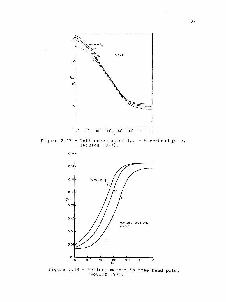
Figure 2.17 - Influence factor I,, - Free (Poulos 1971).

-head pile,

Figure 2.18 - Maximum moment in free-head pile, (Poulos 1971).

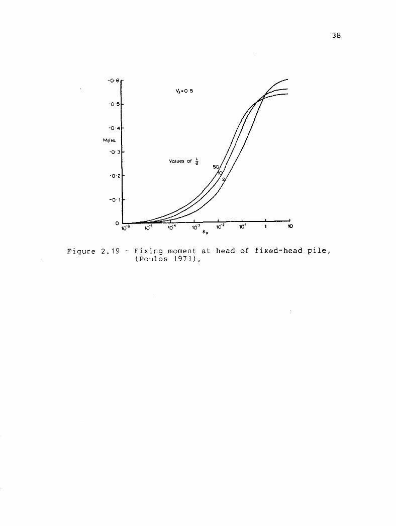
Figure 2.19 - Fixing moment at head of fixed-head pile, (Poulos 1971).

Table 2.1: Evaluation of the coefficient n , and n,, (Broms 1964a) .

Unconllnd Compressive Strength q,,, tms per square foot

Lees than 0.5

0.5 to 2.0

Larger than 2.0 2

Cosfficlent nl

0.32

0.36

0.40 - Pile Material

I I Coefflclent na

Table 2.2: Coefficient of horizontal subgrade reaction k , (Reese et.al 1974).

Steel

Concrete

Wood

TERZAGHI'S VALUES OF k FOR SUBMERGED SAND

1.00

1.15

1.30

R e l a t i v e D e n s i t y Loose Medi um - Dense

3 Range o f Values o f k ( l b s / i n ) 2.6 - 7 .7 7.7 - 26 26 - 51

RECOMMENDED VALUES OF k FOR SUBMERGED SAND

( S t a t i c and C y c l i c Loading)

R e l a t i v e D e n s i t y Loose Med i um

3 Recommended k ( l b s l i n ) 20 60

Dense

125

Table 2.3: Coefficients and equations for Matlock-Reese hand solution, (Matlock-Reese 1 9 6 1 ) .

3 . CALCULATIONS

3.1 Introduction

In this chapter the deflection at ground surface and

maximum moment for a certain pile will be calculated by the

previously described methods. First the parameters for both

the soil and pile are given and the results of the

calculations for each method are given. Finally a summary of

the calculations is given at the end of the chapter.

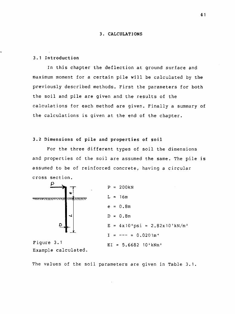
3.2 Dimensions of pile and properties of soil

For the three different types of soil the dimensions

and properties of the soil are assumed the same. The pile is

assumed to be of reinforced concrete, having a circular

cross section.

Figure 3.1 EI = 5.6682 10SkNmZ Example calculated.

The values of the soil parameters are given in Table 3.1.

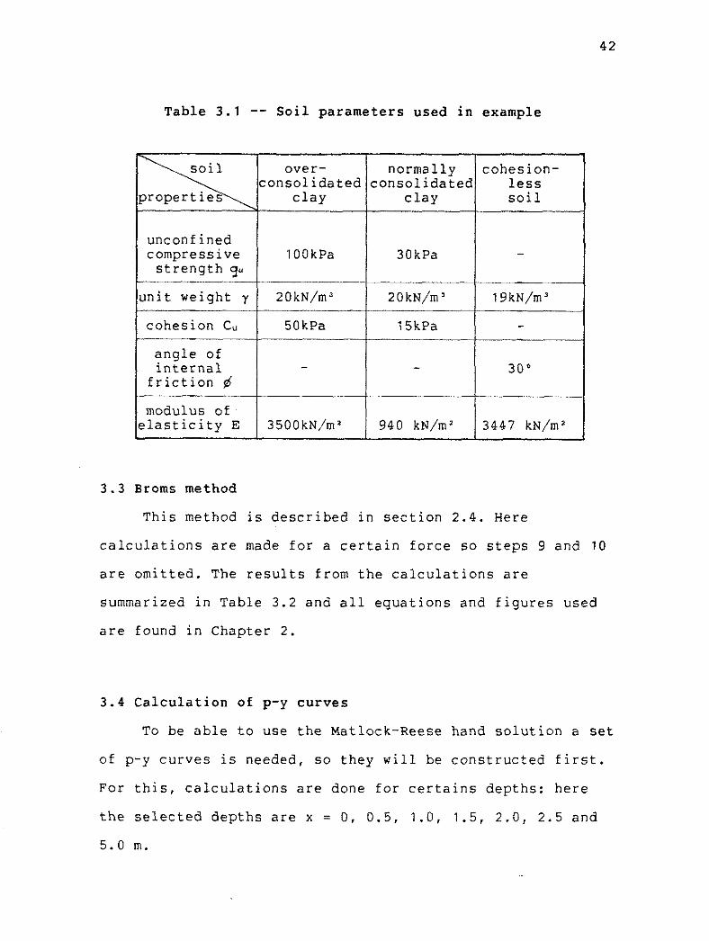
Table 3.1 -- Soil parameters used in example

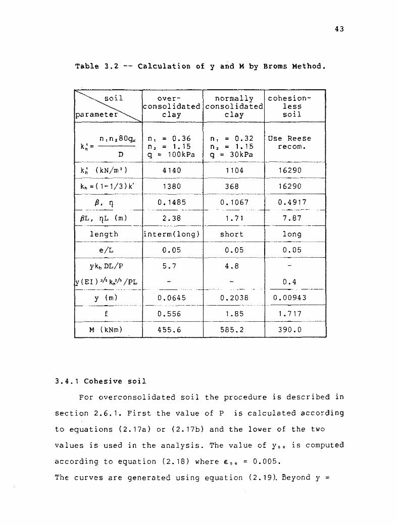
3.3 Broms method

This method is described in section 2.4. Here

calculations are made for a certain force so steps 9 and 10

are omitted. The results from the calculations are

summarized in Table 3.2 and all equations and figures used

are found in Chapter 2.

3.4 Calculation of p-y curves

To be able to use the Matlock-Reese hand solution a set

of p-y curves is needed, so they will be constructed first.

For this, calculations are done for certains depths: here

the selected depths are x = 0, 0.5, 1.0, 1.5, 2.0, 2.5 and

5.0 m.

over- consolidated

clay

normally consolidated

clay

30kPa

~

2 0 kN/m '

15kPa

- ..

940 kN/m2

unconfined compressive strength 9 -

unit weight y -.

cohesion Cu

angle of internal

friction 6

modulus of elasticity E

cohesion- less soil

-

1 9kN/m3

-

30'

3447 kN/m2

lOOkPa

--

20kN/m3

5OkPa

-

3500kN/m2

43

Table 3.2 -- Calculation of y and M by Broms Method.

3.4.1 Cohesive soil

For overconsolidated soil the procedure is described in

section 2.6.1. First the value of P is calculated according

to equations (2.17a) or (2.17b) and the lower of the two

values is used in the analysis. The value of y s O is computed

according to equation (2.18) where E , , = 0.005.

The curves are generated using equation (2.19). Beyond y =

n,n280q, k; =

D

k; (kN/m3 )

kh=(l-1/3)k1

@ I 'I

normally consolidated

clay

n, = 0.32 n, = 1.15 q = 30kPa

1104

368

0.1067 - ~

1.71

short

over- consolidated

clay

n, = 0.36 n, = 1.15 q = lOOkPa

4140

1380

0.1485

cohesion- less soil

Use Reese recom.

16290 -.

16290

~. 0.4917

7.87

long

f

M (kNm)

@L, qL (m) --

length -

e/L

Y kh DL/P

y ( EI ) 3/s k$/' /PL

y (m)

2.38

interm(1ong)

0.05 ~. .-

5.7

-

0.0645

0.05 0.05 ~.

4.8

- .-

0.2038

1.717

390.0

0.556

455.6

-

0.4 -

0.00943

1.85 --

585.2

16y,,, p = p, for all values of y.

The values of p versus y are given in Table 3.3 for

overconsolidated soil and plotted in Figure 3.2.

Table 3.3 - - Calculation of p for each depth and deflection Overconsolidated clay (unit kN/m)

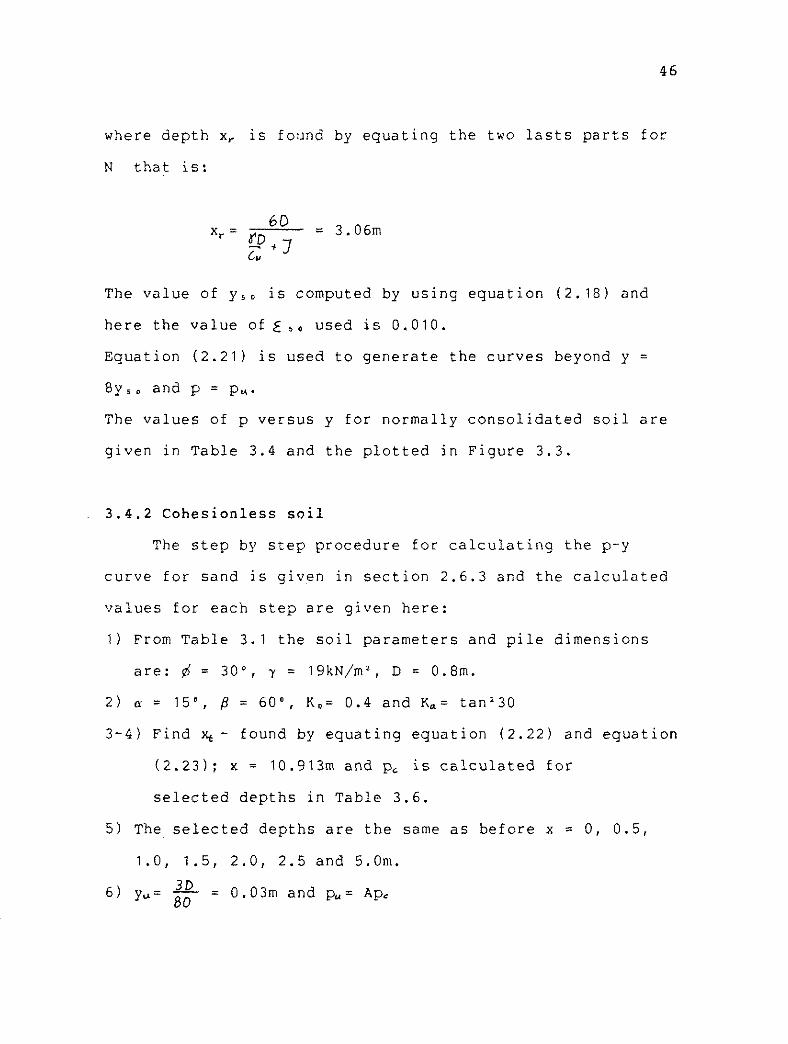
For normally consolidated clay the procedure is given

in section 2.6.2 and equation (2.20) is used for calculation

of p, where:

3 very near the surface

rr, X N p = 3 + - + J- from surface fo depth x, C u D

9 below depth x, i

OSE 082 012 Ofi I DL 0

'(V/NY) d 'a2uelsTsaJ TTOS

where depth x, is found by equating the two lasts parts for

N that is:

The value of y,, is computed by using equation (2.18) and

here the value of E , , used is 0.010.

Equation (2.21) is used to generate the curves beyond y =

8y5, and p = p,.

The values of p versus y for normally consolidated soil are

given in Table 3.4 and the plotted in Figure 3.3.

3.4.2 Cohesionless soil

The step by step procedure for calculating the p-y

curve for sand is given in section 2.6.3 and the calculated

values for each step are given here:

1 ) From Table 3.1 the soil parameters and pile dimensions

are: d = 30°, y = 19kN/m2, D = 0.8m.

2) cr = 15', B = 6O0, K O = 0.4 and K,= tanz30

3-4) Find x, - found by equating equation (2.22) and equation (2.23); x = 10.913m and p, is calculated for

selected depths in Table 3.6.

5 ) The selected depths are the same as before x = 0, 0.5,

1.0, 1.5, 2.0, 2.5 and 5.0m.

3 D 6) yu= - = 0.03m and p,= Ap, 80

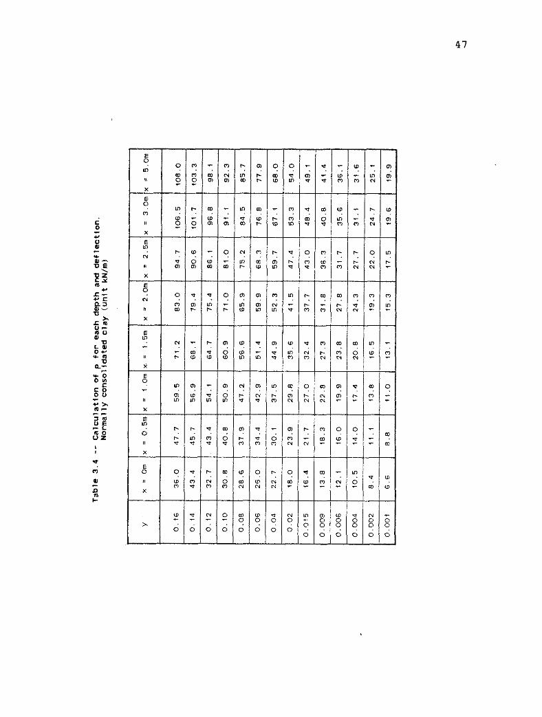
D - - 7 ) Ym= 60 - 0.0 133m and p,= Bp,

where A and B are taken from Figure 2.10 and given in

Table 3.5.

8) The slope of the initial portion of the p-y curve is k,,x

where k,= 16290kN/m3.

9) Between points k and m equation (2.25) is used to

generate the points (see Figure 2.12).

10) Constants m, n, C, y are calculated for each depth and

they are given in Table 3.6.

The p-y curves for cohesionless soil are given in Figure

3.4.

Table 3 . 5 -- Coefficient A and B from Figure 2.13

depth x

0.0

0.5 -- -

1.0

1.5

2.0

2.5 .-

5.0

x /D

0.000

0.625 -.

1.250

1.875

2.500 - 3.125

..

6.250

A

2.87

2.38

1.95

1.57

1.22

1.00

0.88

B

-

2.14

1.78

1.38

1 . 1 1

0.84 P

0.68

0.50

OSE 082 012 Oh1 OL 0

'(w/NY) d 'a3uelsTsaJ TTOS

3.5 Matlock-Reese hand solution

3.5.1'Deflections

The procedure for this method is given in section 2.5.1

and the results of calculations are given in Tables 3.7 to

3.9 for overconsolidated clay, normally consolidated clay

and cohesionless soil respectively. This method is an

iterative procedure. The results of the iterations are

presented in Figures 3.5 to 3.8 and in Tables 3.7 to 3.9.

3.5.2 Moments

Here the moment at the top of the pile is M = 0. The

maximum moment in the pile thus occurs when Am is maximum,

which is Am=0.772 at z = 1.4. The maximum moment for the

three soil types are given below.

Overconsolidated clay:

M,,,= A,PtT = 0.772 200 3.10 = 478.6kNm

at depth x = 1.4T = 4.34m

Normally consolidated clay:

M,,, = 0.772 200 4.25 = 656.2kNm

at depth x = 5.95m

Cohesionless soil:

M,, = 0.772 200 2.15 = 332.0 kNm

at depth x = 3.01m

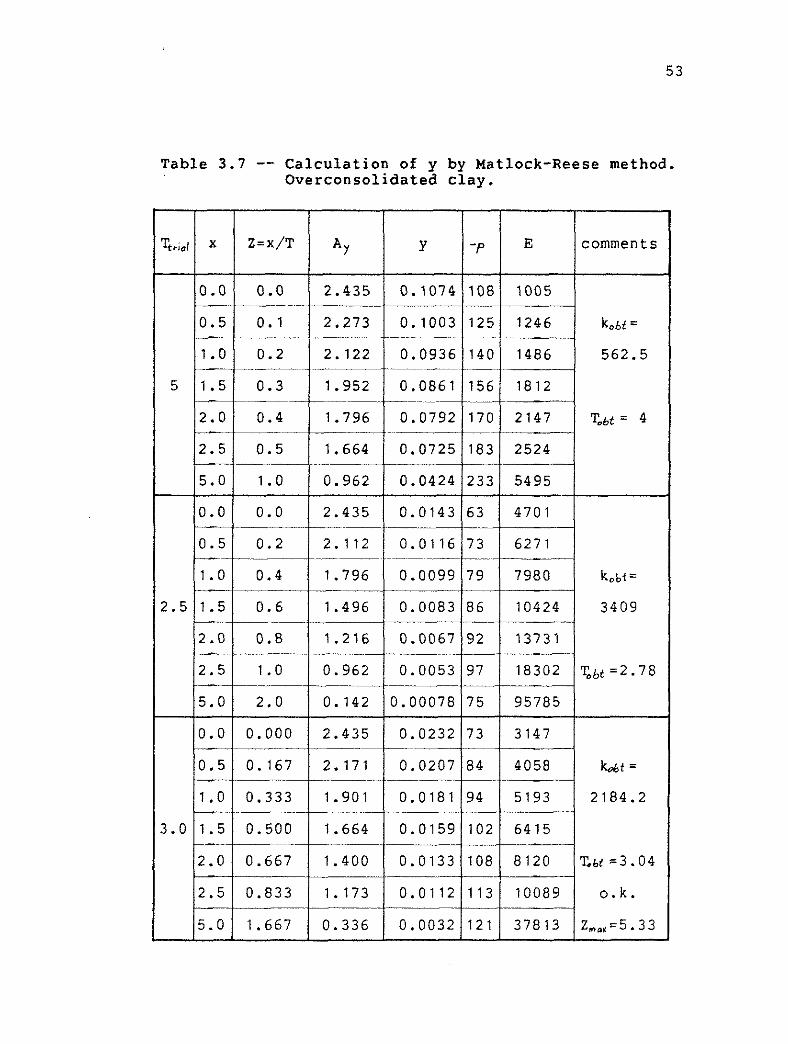
Table 3.7 -- Calculation of y by Matlock-Reese method. Overconsolidated clay.

I

5

2.5

3.0

x

0.0

0.5 - 1.0

1.5 --

2.0

2.5

5 .0

0.0 - 0.5

1.0

1.5

2.0 -- 2.5

5.0

0.0

0 .5

1.0 - 1.5

2.0

2.5

5.0

Z=X/T

0.0 -----

0.1

0.2 --

0.3

0.4

0 .5

1.0

0.0

0.2

0.4

0 .6

0.8

1.0

2.0

0.000 --

0.167

0 .333

0.500 --

0.667

0 .833 -- 1.667

A Y

2.435 1 -

2.273

2.122 .

1.952 - -- 1.796

1.664 -

0.962

2.435

2.112 --

1.796

1.496

1.216

0 .962 - --

0.142

2.435

2.171 -

1.901

1.664 -

1.400

1.173

0.336

Y

0.1074

0.1003 - --

0.0936 - .

0 .0861 - - -.

0.0792

0 .0725

0.0424

0.0143

0.0116

0.0099

0 .0083

0.0067 --

0.0053 -

0.00078

0.0232

0 .0207

0.0181 --

0.0159

0.0133

0.0112 -

0.0032

E

1005 -

1246

1486

1812

2147

2524

5495

4701

6271

7980

10424

13731

18302

95785

3147

4058

5193

6415

8120

10089

37813

-P

108 -- --

125 .-

140 -

156 -

170

183

233

63 -

73

79

8 6

92

97

7 5

73

84

94

102

108

113

121

comments

kobt =

562.5

T,bt = 4

kobt =

3409

T,bt=2.78

k t =

2 184.2

%bt-3.04

0.k.

Z,.,=5.33

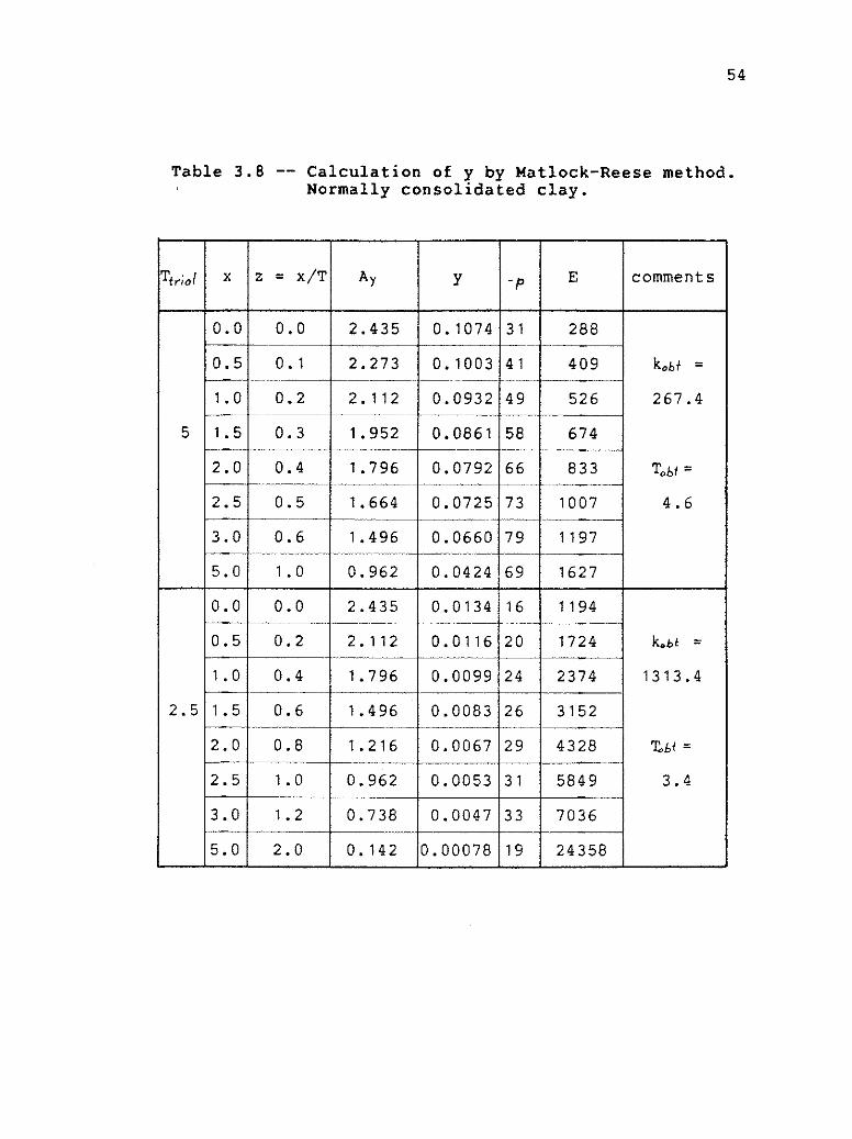
Table 3.8 -- Calculation of y by Matlock-Reese method. Normally consolidated clay.

T o x

0.0

0 . 5

z = x/T

0 . 0

0.1 ~ ~ ~~~-

267 .4

T,bf =

4 . 6

k.bt =

1313 .4

Zb t =

3.4

E

2 8 8

4 0 9 .

1.0 0.2 2 .112 0 .0932 4 9 5 2 6 . -

5 1.5 0 . 3 1.952 0 .0861 5 8

A y

2 . 4 3 5

2 .273 --

comments

kobt =

~. ~ ~

Y

0.1074

0 .1003 -~ . ---

7 0 3 6

2 4 3 5 8

- P

3 1 --

4 1

6 7 4

3 . 0

5 .0

1.2 -- 2.0

2 . 0 0.4

3 3

1 9

0 . 7 3 8

0 . 1 4 2

1.796 -

1.664 2.5

0 .0047

0 .00078

~~.~~

0.5

0 .0792

0 . 0 7 2 5

1197

1 6 2 7

1194 -.

1724

2 3 7 4

3 1 5 2

4 3 2 8

5 8 4 9

3 .0 - 5.0

0.0

0 . 5

1.0

6 6 ~

7 3

0 . 6 1 .496 0 . 0 6 6 0 7 9

8 3 3 ~~ --.-

1007

~~~

1 .0

0.0 ~ . .

0 . 2 .

0.4

2 .5

0 . 9 6 2

2 .435 ~~

2 6 .-

3 1

1.496 - -

1.5 -.

2 .0

2 .5

0 .0424

0 .0134

0 .0083 ~.

0.6

0 .8

1.0

~-

6 9

1 6 .

20

24

2.112

. 1.796

1.216

0 .962

0 . 0 1 1 6

0 . 0 0 9 9

0 . 0 0 6 7 2 9

0 .0053

Table 3.8 -- continued

-P

27

34 -

42

48

55

60 -

64

E

409 --.

559

754

949

1204 ....

1463

1758 -..--

2609

I

4.25

comments

k.bf =

419.4

'Gbt =

4.23 ok

Z ~ . X =

3.76

x

0.0

0 .5 -.

1.0 .

1.5 -~ 2.0

--- 2 .5

----

3.0

5 .0

= x/T

0.0 ~-

0.1176

0.2353 ~p

0.3529

0.4706

0.5882 ~

0.7059

1.1765

A y

2.435 -

2.245 ~

2 .056 -.

1.869

1.689

1.513

1.345

0.764

Y

0.0660

0.0608 ----

0.0557

0.0506 -

0.0457 --

0.0410 ~

0.0365 -

0 . 0 2 0 7 5 4

Table 3.9 -- Calculation of y by Matlock-Reese method. Cohesionless soil.

comments

k o b f =

1692

T o b t =

3.20

k , b f =

9230

T,bt=

2.28

kobt =

11875

T,M =2.17

&~.ar =

7.44

T

5

2.5

2.15

x

0.0

0 .5

1.0

1.5

2.0

2.5

0.0 - 0.5 .-

1.0

1.5

2.0

2.5

0 .0

0.5

1.0

1.5 - 2.0

2.5

= x/T

0.0

0 .1 ~

0 .2

0.3 - ~ -

0 .4

0.5

0 .0

0.2 ---- ~

0.4 - - ..

0 .6

0.8

1.0

0.0

0 .2326 -

0.4651

0.6977

0.9302

1.1628

AI

2.435

2.273

2.112

1.952 ~~

1.796

1.644

2 .435 --

2.112 ~-

1.796

1.496 ~

1 .216

0.962

2 .435

2.0598 - 1.6970

1.3563 -

1.0486

0 .7797

Y

0.1074

0.1003

0.0932

0.0861

0 . 0 7 9 2 2 7 6

0 .0725

0.0134

0.0116 - 0.0099

0.0083 ~

0.0067 ~...

0.0053

0.0085 -

0.0072

0.0060

0.0048 --

0.0037

0.0027

- P

0

70

150

224

328

0

50

95

135

147

155

0

44

80

111

123

130

E

0 -

697

1608 ~-

2599

3487

4530

0

4310

9596

16364 ~

21940 .

29245

0

6111

13445

23319

3 -

m -

Final T = 2.15 m N - -

- - -

R Overconsolidated clay

@ Normally consolidated clay

A Cohesionless s o i l 0

0 1 2 3 11 5

T - t r i e d (rn)

Figure 3.5 - Interpolation for final value of relative stiffness factor.

3.6 Poulos method

This method is described in section 2 . 7 and all graphs

needed for this Calculations are given there. The results of

the calculations are given in Table 3 .10 .

Table 3.10 - Calculation of y and M by Poulos method.

Ep Ip ( kNm2 ) -

E (kN/m2)

L (m) ~ ~~.~

K e -~

L/D -.

IYP

y (m) . ~ .

M/PL - -

M (kNm)

cohesion- less soil

5 . 6 6 10 ' ~ ~

3 4 4 7 -. . -

1 6 - .

0 . 0 0 2 5 1

20 ~... .

6 . 8 -.

0 .0247 -

0 . 0 6 4

2 0 4 . 8

over- consolidated

clay

5 . 6 6 10 '

3500

1 6

0 .00247

2 0 ~

6 . 8

0 .0242

0 . 0 6 3

2 0 1 . 6

normally consolidated

clay

5 . 6 6 10 ' ~ ~,.

940 -

1 6 -~

0 .00920 .

20

5 . 0

0 . 0 6 6 5

0 . 1 0 3

3 3 0 . 7

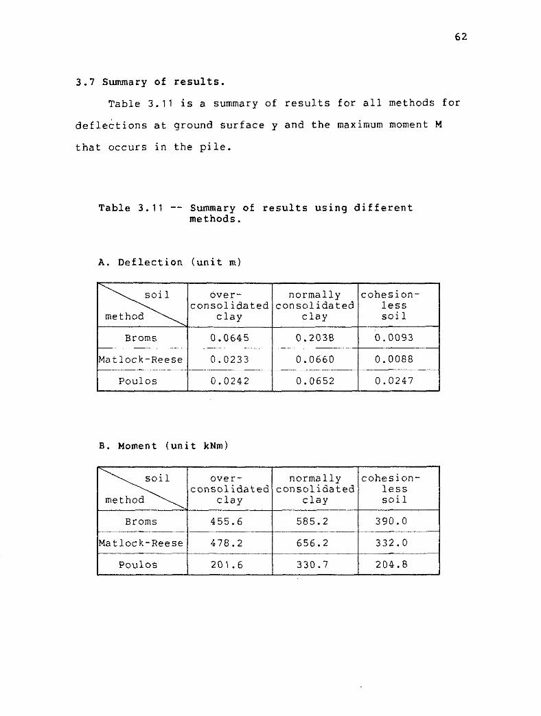
3.7 Summary of results.

Table 3.11 is a summary of results for all methods for

deflections at ground surface y and the maximum moment M

that occurs in the pile.

Table 3.11 -- Summary of results using different methods.

A . Deflection (unit m)

B. Moment (unit kNm)

cohesion- less soil

0 . 0 0 9 3

0 . 0 0 8 8 ~- 0.0247

normally consolidated

clay

0 .2038 ~

0 . 0 6 6 0 ~~-~

0 . 0 6 5 2

over- consolidated

clay

Broms

Matlock-Reese

Poulos

cohesion- less soi 1

3 9 0 . 0

3 3 2 . 0

204 .8

0 .0645 -

0 . 0 2 3 3

0 .0242

normally consolidated

clay

585.2

over- consolidated

clay

Broms 455.6

Matlock-Reese

Poulos

4 7 8 . 2

2 0 1 . 6

6 5 6 . 2 -

3 3 0 . 7

4. DISCUSSION OF RESULTS

4.1 Introduction

In the two previous chapters three different methods

were introduced for calculating deflection and maximum

moment for laterally loaded piles, and example calculations

were presented in Chapter 3. A summary of the results is

given in Table 3.11. In this chapter an explanation of the

results will be sought.

4.2 Cohesionless soil

For cohesionless soil the deflection calculated by the

Broms method and Matlock-Reese method compare fairly well

with each other but Poulos method gives over 2 times greater

values. The moment calculated by Poulos method is lower than

calculated by the other methods. The explanation lies in

that for the Poulos method a constant value of Youngs

modulus E is used which is not valid for cohesionless soil.

When constant value of Youngs modulus is used the subgrade

reaction method agrees better with test results, for example

Gleser result, than does the elastic solution with constant

E (Pise 1972). This is true for both deflections and

moments.

Using an increasing modulus E of the soil with depth

is more realistic than using a constant value. But an

elastic solution with variable E equivalent to the Mindlin

solution, which Poulos method is based on, for constant E

is not available so an approximate analysis must be used, E

= Nhx, where E and kh have the same rate of increase with

depth. Solutions based on varying E also give better

agreement with the results of Gleser than do solutions for

constant E . The fact that, as shown by Pise, the subgrade reaction solution gives better agreement with Gleser's

results than elastic solution for constant E, stems from the

use of varying k rather from the superiority of the

subgrade reaction approach. (Poulos 1 9 7 2 ) .

Uncertainities in determining E remain the same as in

determining the modulus of subgrade reaction (Pise 19721.

4.3 Cohesive soil

For cohesive soil the deflections calculated by the

Matlock-Reese method and the Poulos method compare fairly

well. On the other hand the moments calculated by the Broms

method and the Matlock-Reese method compare fairly well, and

those calculated by Poulos are much lower. The deflections

calculated by the Broms method are 2.5 to 3 greater higher

than calculated by the other two methods. In the following

paragraphs some points are mentioned that might explain this

difference.

Broms (1964) says that deflection depends primarily on

the dimensionless length factor j3L. He gives two equations

to calculate deflections at ground surface for an

unrestrained pile, one for BL less than 1.5 and another for

PL greater than 2.5, that is:

BL < 1.5 4P( l+1 .5?) yo =

K D L

He then shows that the lateral deflection y, at the ground

surface can be expressed as a function of the dimensionless L

quantity y,kD --- versus dimensionless length PL. It seems D

that for Bt between 1.5 and 2.5 an extrapolation is made

between these equations (see Figure 2.5) . The value of the

dimensionless length PL for the cases calculated here are in

this range.

Also, for BL less than 1.5 the stiffness of the pile is

not taken into account for calculation of deflection except

for selecting the equation.

When Broms compared this method to case histories for

various types of soil and degrees of end restraint he found

that the measured lateral deflections at the ground surface

varied from between 0.5 to 3.0 times the calculated

deflections. For short piles the lateral deflections are

inversely proportional to the assumed coefficient of

horizontal subgrade reaction, k,,, and thus also to the

measured average unconfined compressive strength of the

supporting soil. Thus small variations in q will have large

effects on the calculated lateral deflections. Also,

agreement between calculated and measured lateral

deflections improves with decreasing shear strength of the

soil.

Broms does not describe any case histories for

unrestrained (free-head) concrete piles driven into the

soil.

When comparing elastic solution and subgrade reaction

method, relationship between the Young's modulus and the

coefficient of horizontal subgrade reaction has to be

established. Poulos does this by equating the elastic and

subgrade reaction for displacement of a stiff clay and

states that this is the most accurate way. And then compares

his solution with the one by Hetenyi (1946). There all the

values from the subgrade reaction are greater than from the

elastic theory. The difference becomes increasingly marked

as the stiffness of the pile descreases. Comparisons between

the corresponding solutions for moments give that the

largest difference between the two solutions again occurs

for relativly flexible piles, for which the subgrade

reaction overestimates the moments. However,' the two methods

are in reasonable agreement for stiff piles and, in general,

the agreement is better than for displacement.

Kosics points out that Vesic states that the subgrade

reaction method underestimates the deflections, while Poulos

states that it overestimates them. The difference lies in

the different basis of relating k h and E values. Also, the

disadvantages of the subgrade reaction method is that k h

depentls upon the pile properties as well as the soil

properties. And that could mean that the same k h should not

be used for piles of different stiffnesses. Consequently,

the results from a lateral load test on a particular pile

cannot be directly applied to the analysis of other piles or

piles groups with different conditions of end restraints

although the soil conditions are the same. In order to

obtain agreement between elastic solution and subgrade

reaction solution, different k should be used for piles of

different stiffnesses. The elastic solution also has its

limitations. The method is limited to constant E value. The

term E is not only going to vary from point to point in the

soil mass, but also at a given point it will vary with

stress conditions at that point. Also, the Mindlin solution

is used and that includes the assumption that the soil is

capable of resisting tensile stresses on one side of the

pile. This assumption would not be valid in the critical

zone near the ground surface.

References

Broms, B., 1964a. Lateral Resistance of Piles in Cohesive Soil. JSMFD, ASCE, Vol. 90, NOSM2, p27-63.

Broms, B., 1964b. Lateral Resistance of Piles in Cohesronless Soil. JSMFD, ASCE, Vol. 90, NoSM3, p123-156.

Brsms, B., 1965. Design of Laterally Loaded Piles. JSMFD, ASCE, Vol. 91, NoSM3, p79-99.

DeBeer, E., 1977. Piles Subjected to Static Lateral Loads. Proc. 10th ICSMFE, Tokyo 1977, Special Session NolO.

Hetenyi, M., 1946. Beams on Elastic Foundation. Univ. of Michigan Press, Ann Arbor Mich Oxford Univ. Press, London England 1946.

Kocsis, P., 1972. Discussion of Behaviour of Laterally Loaded Pi1es:l-Single Piles. JSMFD, ASCE, Vol. 98, NoSM1, p124-125.

Matlock, H., 1970. Correlation for Design of Laterally Loaded Piles in Soft Clay. Proc. 2nd Annual Offshore Technology Conf., Houston Texas, Vol. 1 , p577-594.

Matlock, H., and Reese, L.C., 1960. Generalized Solution for Laterally Loaded Piles. JSMFD, ASCE, Vol. 86 NoSM5, p63-9 1.

Matlock, H., and Reese, L.C., 1961. Foundation Analysis of Offshore Pile Supported Structure. Proc. 5th ICSMFE, July 1961, p91-97.

McClelland, B., and Focht, J.A., 1958. Soil Modulus for Laterally Loaded Piles. ASCE, Transaction 1958, Vol. 123, p1049.

New York State Department of Transportation, Laterally Load Capacity of Vertical Pile Groups. Eng R & D Bureau Albany New York, Research Report 47, April 1977, pp44.

Pise, P.J., 1972. Discussion of Behaviour of Laterally Loaded Piles: I-Single piles. JSMFD, ASCE, Vol. 98, NoSM2, p225-226.

Poulos, H.G., 1971. Behaviour of Laterally loaded Pi1es:I -Single piles. JSMFD, ASCE, ~01.97, NoSM5, p711-731.

~oulos, H.G., 1972. Closure to Behaviour of Laterally Loaded Piles:I-Single piles. JSMFD, ASCE, Val. 98, NoSM11, p1269 -1272.

Reese, L.C., Cox, W.R., and Koop, F.D., 1974. Analysis of Laterally Loaded Plles in Sand. Proc. 6th Annual Offshore Technology Conf., Houston Texas 1974, p473-483.

Reese, L.C., and Welch, R.C., 1975. Lateral Loading of Deep Foundation in Stiff Clay. JGTD, ASCE, Vol. 101, p633-649

Terzaghi, K., 1955. Evaluation of Coefficient of Subgrade Reaction. Geotechnique, Vol. 5, Dec. 1955, p297-326.

Timoshenko, S.P., and Gere, J.M., 1961. Theory of Elastic Stability. 2nd Edition, McGraw Hill Book Co., New York 1961.

Vesic, A.S., 1977. Design of Pile Foundation. NCHRP Synthesis of Highway Practice 42, 68pp.

Wilson, W.E., 1972. Discussion of Behaviour of Laterally Loaded Pi1es:I-Single Piles. JSMFD, ASCE, vol. 98, NoSM3, p298-299.