30 years of adaptive neural networks: perceptron, Madaline ...widrow/papers/j199030years.pdf · 30 Years of Adaptive Neural Networks: Perceptron, Madaline, and Backpropagation BERNARD

30 Years of Adaptive Neural Networks: Perceptron, Madaline, and Backpropagation

BERNARD WIDROW, FELLOW, IEEE, AND MICHAEL A. LEHR

Fundamental developments in feedfonvard artificial neural networks from the past thirty years are reviewed. The central theme of this paper is a description of the history, origination, operating characteristics, and basic theory of several supervised neural network training algorithms including the Perceptron rule, the LMS algorithm, three Madaline rules, and the backpropagation technique. These methods were developed independently, but with the perspective of history they can a / / be related to each other. The concept underlying these algorithms is the “minimal disturbance principle,” which suggests that during training it is advisable to inject new information into a network in a manner that disturbs stored information to the smallest extent possible.

I . INTRODUCTION

This year marks the 30th anniversary of the Perceptron rule and the LMS algorithm, two early rules for training adaptive elements. Both algorithms were first published in 1960. In the years following these discoveries, many new techniques have been developed in the field of neural networks, and the discipline is growing rapidly. One early development was Steinbuch’s Learning Matrix [I], a pattern recognition machine based on linear discriminant functions. At the same time, Widrow and his students devised Madaline Rule I (MRI), the earliest popular learning rule for neural networks with multiple adaptive elements [2]. Other early work included the “mode-seeking” technique of Stark, Okajima, and Whipple [3]. This was probably the first example of competitive learning in the literature, though it could be argued that earlierwork by Rosenblatt on “spon- taneous learning” [4], [5] deserves this distinction. Further pioneering work on competitive learning and self-organization was performed in the 1970s by von der Malsburg [6] and Grossberg [7l. Fukushima explored related ideas with his biologically inspired Cognitron and Neocognitron models [8], [9].

Manuscript received September 12,1989; revised April 13,1990. This work was sponsored by SDI0 Innovative Science and Tech- nologyoffice and managed by ONR under contract no. N00014-86- K-0718, by the Dept. of the Army Belvoir RD&E Center under con- tracts no. DAAK70-87-P-3134and no. DAAK-70-89-K-0001, by a grant from the Lockheed Missiles and Space Co., by NASA under contract no. NCA2-389, and by Rome Air Development Center under contract no. F30602-88-D-0025, subcontract no. E-21-T22-S1.

The authors are with the Information Systems Laboratory, Department of Electrical Engineering, Stanford University, Stan- ford, CA 94305-4055, USA.

IEEE Log Number 9038824.

Widrow devised a reinforcement learning algorithm called “punish/reward” or ”bootstrapping” [IO], [ I l l in the mid-1960s. This can be used to solve problems when uncer- tainty about the error signal causes supervised training methods to be impractical. A related reinforcement learning approach was later explored in a classic paper by Barto, Sutton, and Anderson on the “credit assignment” problem [12]. Barto et al.’s technique is also somewhat reminiscent of Albus’s adaptive CMAC, a distributed table-look-up system based on models of human memory [13], [14].

In the 1970s Grossberg developed his Adaptive Reso- nance Theory (ART), a number of novel hypotheses about the underlying principles governing biological neural systems [15]. These ideas served as the basis for later work by Carpenter and Grossberg involving three classes of ART architectures: ART 1 [16], ART 2 [17], and ART 3 [18]. These are self-organizing neural implementations of pattern clustering algorithms. Other important theory on self-organizing systems was pioneered by Kohonen with his work on feature maps [19], [201.

In the early 1980s, Hopfield and others introduced outer product rules as well as equivalent approaches based on the early work of Hebb [21] for training a class of recurrent (signal feedback) networks now called Hopfield models [22], [23]. More recently, Kosko extended some of the ideas of Hopfield and Grossberg to develop his adaptive Bidirec- tional Associative Memory (BAM) [24], a network model employing differential as well as Hebbian and competitive learning laws. Other significant models from the past decade include probabilistic ones such as Hinton, Sejnowski, and Ackley‘s Boltzmann Machine [25], [26] which, to over- simplify, is a Hopfield model that settles into solutions by a simulated annealing process governed by Boltzmann statistics. The Boltzmann Machine i s trained by a clever two- phase Hebbian-based technique.

While these developments were taking place, adaptive systems research at Stanford traveled an independent path. After devising their Madaline I rule, Widrow and his students developed uses for the Adaline and Madaline. Early applications included, among others, speech and pattern recognition [27], weather forecasting [28], and adaptive controls [29]. Work then switched to adaptive filtering and adaptive signal processing [30] after attempts to develop learning rules for networks with multiple adaptive layers were unsuccessful. Adaptive signal processing proved to

0018-9219/90/0900-1415$01.00 0 1990 IEEE

PROCEEDINGS OF THE IEEE, VOL. 78, NO. 9, SEPTEMBER 1990 1415

bea fruitful avenue for research with applications involving adaptive antennas [311, adaptive inverse controls [32], adaptive noise cancelling [33], and seismic signal processing [30]. Outstanding work by Lucky and others at Bell Laboratories led to major commercial applications of adaptive filters and the L M S algorithm to adaptive equalization in high-speed modems [34], [35] and to adaptive echo cancellers for long- distance telephone and satellite circuits [36]. After 20 years of research in adaptive signal processing, the work in Wid- row’s laboratory has once again returned to neural networks.

The first major extension of the feedforward neural network beyond Madaline I took place in 1971 when Werbos developed a backpropagation training algorithm which, in 1974, he first published in his doctoral dissertation [371.’ Unfortunately, Werbos’s work remained almost unknown in the scientific community. In 1982, Parker rediscovered the technique [39] and in 1985, published a report on it at M.I.T. [40]. Not long after Parker published his findings, Rumelhart, Hinton, and Williams [41], [42] also rediscovered the techniqueand, largelyasaresultof theclear framework within which they presented their ideas, they finally suc- ceeeded in making it widely known.

The elements used by Rumelhart et al. in the backpropagation network differ from those used in the earlier Mada- line architectures. The adaptive elements in the original Madaline structure used hard-limiting quantizers (signums), while the elements in the backpropagation network use only differentiable nonlinearities, or “sigmoid” functions.2 In digital implementations, the hard-limiting quantizer is more easily computed than any of the differentiable nonlinearities used in backpropagation networks. In 1987, Widrow,Winter,and Baxter looked backattheorig- inal Madaline I algorithm with the goal of developing a new technique that could adapt multiple layers of adaptive elements using the simpler hard-limitingquantizers. The result was Madaline Rule II [43].

David Andes of U.S. Naval Weapons Center of China Lake, CA, modified Madaline I I in 1988 by replacing the hard-limiting quantizers in the Adaline and sigmoid functions, thereby inventing Madaline Rule Ill (MRIII). Widrow and his students were first to recognize that this rule i s mathematically equivalent to backpropagation.

The outline above gives only a partial view of the discipline, and many landmark discoveries have not been mentioned. Needless to say, the field of neural networks is quickly becoming a vast one, and in one short survey we could not hope to cover the entire subject in any detail. Consequently, many significant developments, including some of those mentioned above, are not discussed in this paper. The algorithms described are limited primarily to

’Weshould note, however, that in the fieldof variational calculus the idea of error backpropagation through nonlinear systems existed centuries before Werbosfirstthoughttoapplythisconcept to neural networks. In the past 25years, these methods have been used widely in the field of optimal control, as discussed by Le Cun [381.

*The term “sigmoid” i s usually used in reference to monoton- ically increasing “S-shaped” functions, such as the hyperbolic tangent. In this paper, however, we generally use the term to denote any smooth nonlinear functions at the output of a linear adaptive element. In other papers, these nonlinearities go by a variety of names, such as “squashing functions,” ”activation functions,” “transfer characteristics,” or ”threshold functions.”

thosedeveloped in our laboratoryat Stanford, and to related techniques developed elsewhere, the most important of which is the backpropagation algorithm. Section I I explores fundamental concepts, Section Ill discusses adaptation and the minimal disturbance principle, Sections IV and V cover error correction rules, Sections VI and VI1 delve into steepest-descent rules, and Section V l l l provides a summary.

Information about the neural network paradigms not discussed in this papercan beobtainedfromanumberofother sources, such as the concise survey by Lippmann [44], and the collection of classics by Anderson and Rosenfeld [45]. Much of the early work in the field from the 1960s is care- fully reviewed in Nilsson’s monograph [46]. A good view of some of the more recent results i s presented in Rumel- hart and McClelland’s popular three-volume set [471. A paper by Moore [48] presents a clear discussion about ART 1 and some of Crossberg’s terminology. Another resource is the DARPA Study report [49] which gives a very compre- hensive and readable “snapshot” of the field in 1988.

I I . FUNDAMENTAL CONCEPTS

Today we can build computers and other machines that perform avarietyofwell-defined taskswith celerityand reli- ability unmatched by humans. No human can invert matri- ces or solve systems of differential equations at speeds rivaling modern workstations. Nonetheless, many problems remain to be solved to our satisfaction by any man- made machine, but are easily disentangled by the percep- tual or cognitive powers of humans, and often lower mam- mals, or even fish and insects. No computer vision system can rival the human ability to recognize visual images formed by objects of all shapes and orientations under a wide range of conditions. Humans effortlessly recognize objects in diverse environments and lighting conditions, even when obscured by dirt, or occluded by other objects. Likewise, the performance of current speech-recognition technology pales when compared to the performance of the human adult who easily recognizes words spoken by different people, at different rates, pitches, and volumes, even in the presence of distortion or background noise.

The problems solved more effectively by the brain than by the digital computer typically have two characteristics: they are generally ill defined, and they usually require an enormous amount of processing. Recognizing the character of an object from its image on television, for instance, involves resolving ambiguities associated with distortion and lighting. It also involves filling in information about a three-dimensional scene which i s missing from the two- dimensional image on the screen. An infinite number of three-dimensional scenes can be projected into a two- dimensional image. Nonetheless, the brain deals well with this ambiguity, and using learned cues usually has little difficulty correctly determining the role played bythe missing dimension.

As anyone who has performed even simple filtering oper- ations on images is aware, processing high-resolution images requires a great deal of computation. Our brains accomplish this by utilizing massive parallelism, with mil- lions and even billions of neurons in partsof the brain work- ing together to solve complicated problems. Because solid- state operational amplifiers and logic gates can compute

1416 PROCEEDINGS OF THE IEEE, VOL. 78, NO. 9, SEPTEMBER 1990

1

many orders of magnitude faster than current estimates of the computational speed of neurons in the brain, we may soon be able to build relatively inexpensive machines with the ability to process as much information as the human brain.Thisenormous processing powerwill do l itt leto help US solve problems, however, unless we can utilize it effectively. For instance, coordinating many thousands of pro- cessors, which must efficiently cooperate to solve a problem, is not a simple task. If each processor must be programmed separately, and if all contingencies associated with various ambiguities must be designed into the soft- ware, even a relatively simple problem can quickly become unmanageable. The slow progress over the past 25 years or so in machinevision and otherareasofartificial intelligence i s testament to the difficulties associated with solving ambiguous and computationally intensive problems on von Neumann computers and related architectures.

Thus, there i s some reason to consider attacking certain problems by designing naturally parallel computers, which process information and learn by principles borrowed from the nervous systems of biological creatures. This does not necessarily mean we should attempt to copy the brain part for part. Although the bird served to inspire development of the airplane, birds do not have propellers, and airplanes do not operate by flapping feathered wings. The primary parallel between biological nervous systems and artificial neural networks is that each typically consists of a large number of simple elements that learn and are able to col- lectively solve complicated and ambiguous problems.

Today, most artificial neural network research and application is accomplished by simulating networks on serial computers. Speed limitations keep such networks relatively small, but even with small networks some surprisingly difficult problems have been tackled. Networks with fewer than 150 neural elements have been used successfully in vehicular control simulations [50], speech generation [51], [52], and undersea mine detection [49]. Small networks have also been used successfully in airport explosive detection [53], expert systems [54], [55], and scores of other applications. Furthermore, efforts to develop parallel neural network hardware are meeting with some success, and such hardware should be available in the future for attacking more difficult problems, such as speech recognition [56], [57l.

Whether implemented in parallel hardware or simulated on a computer, all neural networks consist of a collection of simple elements that work together to solve problems. A basic building block of nearly all artificial neural networks, and most other adaptive systems, is the adaptive linear combiner.

A. The Adaptive Linear Combiner

The adaptive linear combiner i s diagrammed in Fig. 1. Its output i s a linear combination of i t s inputs. In a digital implementation, this element receives at time k an input signal vector or input pattern vector X k = [x,, x l t , xzk, . . 1 , x,,]' and a desired response dk, a special input used to effect learning. The components of the input vector are weighted by a set of coefficients, the weight vector Wk = [wok, wlk, wZt, * . . , w,~]'. The sum of the weighted inputs is then computed, producing a linear output, the inner product sk = XLWk. The components of X k may be either

Input

Vector output

: / I nk

Error t 1 dk

Desired Response Wk

Weight Vector

Fig. 1. Adaptive linear combiner.

continuous analog values or binary values. The weights are essentially continuously variable, and can take on negative as well as positive values.

During the training process, input patterns and corresponding desired responses are presented to the linear combiner. An adaptation algorithm automatically adjusts the weights so that the output responses to the input patterns will be as close as possible to their respective desired reponses. In signal processing applications, the most popular method for adapting the weights is the simple LMS (least mean square) algorithm [58], [59], often called the Widrow-Hoff delta rule [42]. This algorithm minimizes the sum of squares of the linear errors over the training set. The linear error t k i s defined to be the difference between the desired response dk and the linear output s k , during presentation k . Having this error signal is necessary for adapting the weights. When the adaptive linear combiner i s embedded in a multi-element neural network, however, an error signal i s often notdirectlyavailableforeach individual linear combiner and more complicated procedures must be devised for adapting the weight vectors. These procedures are the main focus of this paper.

B. A Linear Classifier-The Single Threshold Element

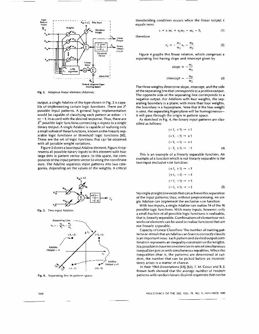
The basic building block used in many neural networks is the "adaptive linear element," or Adaline3 [58] (Fig. 2).

This i s an adaptive threshold logic element. It consists of an adaptive linear combiner cascaded with a hard-limiting quantizer, which is used to produce a binary 1 output, Yk = sgn (sk) . The bias weight wok which i s connected to a constant input xo = + I , effectively controls the threshold level of the quantizer.

In single-element neural networks, an adaptivealgorithm (such as the LMS algorithm, or the Perceptron rule) i s often used to adjust the weights of the Adaline so that it responds correctly to as many patterns as possible in a training set that has binary desired responses. Once the weights are adjusted, the responses of the trained element can be tested by applying various input patterns. If the Adaline responds correctly with high probability to input patterns that were not included in the training set, it i s said that generalization has taken place. Learning and generalization are among the most useful attributes of Adalines and neural networks.

Linear Separability: With n binary inputs and one binary

31n the neural network literature, such elements are often referred to as "adaptive neurons." However, in a conversation between David Hubel of Harvard Medical School and Bernard Wid- row, Dr. Hubel pointed out that the Adaline differs from the biological neuron in that it contains not only the neural cell body, but also the input synapses and a mechanism for training them.

WIDROW AND LEHR: PERCEPTRON, MADALINE, AND BACKPROPACATION 1417

Linear output

Binary output (+L-11

' - _ - - - _ _ - - _ _ _ - - _ _ _ _ _ _ - - I

'k-1- Desired Response Input

(training signal)

Fig. 2. Adaptive linear element (Adaline).

output, a single Adaline of the type shown in Fig. 2 is capable of implementing certain logic functions. There are 2" possible input patterns. A general logic implementation would be capable of classifying each pattern as either + I or -1, in accord with the desired response. Thus, there are 22' possible logic functions connecting n inputs to a single binary output. A single Adaline is capable of realizing only asmall subset of thesefunctions, known as the linearlysep- arable logic functions or threshold logic functions [60]. These are the set of logic functions that can be obtained with all possible weight variations.

Figure3 shows atwo-input Adalineelement. Figure4 represents all possible binary inputs to this element with four large dots in pattern vector space. In this space, the com- ponentsof the input pattern vector liealongthecoordinate axes. The Adaline separates input patterns into two cate- gories, depending on the values of the weights. A critical

Xok= +1

'k

Fig. 3. Two-input Adaline.

Separat ing Line

x z = 3 x , - "0 w2 WZ

Fig. 4. Separating line in pattern space.

thresholding condition occurs when the linear output s equals zero:

s = XlW, + X,W, + WO = 0, (1)

therefore

w 1 x , - -. WO x 2 = --

w2 w2

Figure 4 graphs this linear relation, which comprises a separating line having slope and intercept given by

W slope = -2

intercept = -3.

w 2

w2 (3)

The three weights determine slope, intercept, and the side of the separating line that corresponds to a positive output. The opposite side of the separating line corresponds to a negative output. For Adalines with four weights, the separating boundary is a plane; with more than four weights, the boundary i s a hyperplane. Note that if the bias weight i s zero, the separating hyperplane will be homogeneous- it wil l pass through the origin in pattern space.

As sketched in Fig. 4, the binary input patterns are clas- sified as follows:

(+ I , + I ) + + I

(+I , -1) + + I

(-1, -1) -+ + I

(-1, +I ) + -1 (4)

This is an example of a linearly separable function. An example of a function which i s not linearly separable is the two-input exclusive NOR function:

(+ I , +I) + +I

(+I, -1) -+ -1

(-1, -1) + + I

(-1, +I) + -1 (5)

Nosinglestraight lineexiststhat can achievethisseparation of the input patterns; thus, without preprocessing, no single Adaline can implement the exclusive NOR function.

With two inputs, a single Adaline can realize 14 of the 16 possible logic functions. With many inputs, however, only a small fraction of all possible logic functions i s realizable, that is, linearly separable. Combinations of elements or networks of elements can be used to realize functions that are not linearly separable.

Capacity of Linear C/assifiers:The number of training patterns or stimuli that an Adalinecan learn tocorrectlyclassify i s an important issue. Each pattern and desired output combination represents an inequalityconstraint on the weights. It i s possible to have inconsistencies in sets of simultaneous inequalities just as with simultaneous equalities. When the inequalities (that is, the patterns) are determined at random, the number that can be picked before an inconsis- tency arises i s a matter of chance.

In their 1964 dissertations [61], [62], T. M. Cover and R. J. Brown both showed that the average number of random patterns with random binary desired responses that can be


absorbed by an Adaline i s approximately equal to twice the number of weights4 This i s the statistical pattern capacity C, of the Adaline. As reviewed by Nilsson [46], both theses included an analyticformuladescribingthe probabilitythat such a training set can be separated by an Adaline (i.e., it is linearly separable). The probability i s afunction of Np, the number of input patterns in the training set, and N,, the number of weights in the Adaline, including the threshold weight, i f used:

for N, 5 N,.

In Fig. 5 this formula was used to plot a set of analytical curves, which show the probability that a set of Np random patterns can be trained into an Adaline as a function of the ratio NJN,. Notice from these curves that as the number of weights increases, the statistical pattern capacity of the AdalineC, = 2N,becomesan accurateestimateofthenum- ber of responses it can learn.

Another fact that can be observed from Fig. 5 i s that a

0 8 -

Probability of Linear 0 6 Separability

0 4 -

N,= 15 N,= 5 N,= 2

Np/Nw--Ratio of Input Patterns to Weights

Fig. 5. Probability that an Adaline can separate a training pattern set as a function of the ratio NJN,.

problem is guaranteed to have a solution if the number of patterns i s equal to (or less than) half the statistical pattern capacity; that is, if the number of patterns i s equal to the number of weights. We will refer to this as the deterministic pattern capacityCdof the Adaline. An Adaline can learn any two-category pattern classification task involving no more patterns than that represented by its deterministic capacity,

Both the statistical and deterministic capacity results depend upon a mild condition on the positionsof the input patterns: the patterns must be in general position with respect to the Adaline.’ If the input patterns to an Adaline

Cd = N,.

4Underlying theory for this result was discovered independently by a number of researchers including, among others, Winder [63], Cameron [U], and Joseph [65].

5Patterns are in general position with respect to an Adaline with no threshold weight i f any subset of pattern vectors containing no more than N, members forms a linearly independent set or, equiv- alently, i f no set of N, or more input points in the N,-dimensional pattern space lie on a homogeneous hyperplane. For the more common case involving an Adaline with a threshold weight, general position means that no set of N, or more patterns in the (N, - 1)-dimension pattern space lie on a hyperplane not constrained to pass through the origin [61], [46].

are continuous valued and smoothly distributed (that is, pattern positions are generated by a distribution function containing no impulses), general position i s assured. The general position assumption i s often invalid if the pattern vectors are binary. Nonetheless, even when the points are not in general position, the capacity results represent useful upper bounds.

The capacity results apply to randomly selected training patterns. In most problems of interest, the patterns in the training set are not random, but exhibit some statistical regularities. These regularities are what make generalization possible. The number of patterns that an Adaline can learn in a practical problem often far exceeds its statistical capacity becausethe Adaline isabletogeneralizewithin thetraining set, and learns many of the training patterns before they are even presented.

C. Nonlinear Classifiers

Thelinearclassifier i s limited in itscapacity,andofcourse i s limited to only linearly separable forms of pattern dis- crimination. More sophisticated classifiers with higher capacities are nonlinear. Two types of nonlinear classifiers are described here. The first i s a fixed preprocessing network connected to a single adaptive element, and the other i s the multi-element feedforward neural network.

Polynomial Discriminant Functions: Nonlinear functions of the in.puts applied to the single Adaline can yield nonlinear decision boundaries. Useful nonlinearities include the polynomial functions. Consider the system illustrated in Fig. 6 which contains only linear and quadratic input

Input Pattern VeCtOl

X X l

Binary

Y - output

(+1,-1)

Fig. 6. Adalinewith inputs mapped through nonlinearities.

functions. The critical thresholding condition for this system is

s = WO + XlWl + x:w1, + X1XzW12

+ x;w2* + xzw2 = 0. (7)

With proper choiceof theweights, the separating boundary in pattern space can be established as shown, for example, in Fig. 7.This representsasolutionfortheexclusive NOR

function of (5). Of course, all of the linearly separable functions are also realizable. The use of such nonlinearities can be generalized for more than two inputs and for higher degree polynomial functions of the inputs. Some of the first work in this area was done by Specht [66]-[68] at Stanford in the 1960s when he successfully applied polynomial dis- criminants to the classification and analysis of electrocardiographic signals. Work on this topic has also been done

WIDROW AND LEHR: PERCEPTRON, MADALINE, AND BACKPROPAGATION 1419

Separating Boundary r Madaline I was built out of hardware [78] and used in pat-

tern recognition research. Theweights in this machinewere memistors, electrically variable resistors developed by Widrow and Hoff which are adjusted by electroplating a resistive link [79].

Madaline I was configured in the following way. Retinal inputs were connected to a layer of adaptive Adaline elements, the outputs of which were connected to a fixed logic device that generated the system output. Methods for adapting such systems were developed at that time. An exampleof this kind of network is shown in Fig. 8. TwoAda-

Adaline Output = -1

Adal ine -0 O u t p u t = +1

Fig. 7. Elliptical separating boundary for realizing a function which i s not linearly separable.

by Barron and Barron [69]-[71] and by lvankhnenko [72] in the Soviet Union.

The polynomial approach offers great simplicity and beauty.Through it onecan realizeawidevarietyofadaptive nonlinear discriminant functions by adapting only a single Adaline element. Several methods have been developed for training the polynomial discriminant function. Specht developed a very efficient noniterative (that is, single pass through the training set) training procedure: the polynomial discriminant method (PDM), which allows the polynomial discriminant function to implement a nonpara- metric classifier based on the Bayes decision rule. Other methods for training the system include iterative error-correction rules such as the Perceptron and a-LMS rules, and iterative gradient-descent procedures such as the w-LMS and SER (also called RLS) algorithms [30]. Gradient descent with a single adaptive element is typically much faster than with a layered neural network. Furthermore, as we shall see, when the single Adaline is trained by a gradient descent procedure, it will converge to a unique global solution.

After the polynomial discriminant function has been trained byagradient-descent procedure, theweights of the Adaline will represent an approximation to the coefficients in a multidimensional Taylor series expansion of thedesired response function. Likewise, if appropriate trigonometric terms are used in place of the polynomial preprocessor, the Adaline's weight solution will approximate the terms in the (truncated) multidimensional Fourier series decomposi- tion of a periodic version of the desired response function. The choice of preprocessing functions determines how well a network will generalize for patterns outside the training set. Determining "good" functions remains a focus of current research [73], [74]. Experience seems to indicate that unless the nonlinearities are chosen with care to suit the problem at hand, often better generalization can be obtained from networks with more than one adaptive layer. In fact,onecan view multilayer networks assingle-layer networks with trainable preprocessors which are essentially self-optimizing.

Madaline I

One of the earliest trainable layered neural networks with multiple adaptive elements was the Madaline I structure of Widrow [2] and Hoff (751. Mathematical analyses of Mada- line I were developed in the Ph.D. theses of Ridgway [76], Hoff [75], and Glanz [77]. In the early 1960s, a 1000-weight

Input Pattern Vector

X xiT- - , , & py output

x 1

Fig. 8. Two-Adaline form of Madaline.

lines are connected to an AND logic device to provide an output.

With weights suitably chosen, the separating boundary in pattern space for the system of Fig. 8 would be as shown in Fig. 9. This separating boundary implements the exclusive NOR function of (5).

Separating Lines ,\

o u t p u t = +1

Fig. 9. Separating lines for Madaline of Fig. 8.

Madalines were constructed with many more inputs, with many more Adaline elements in the first layer, and with various fixed logic devices such as AND, OR, and majority-vote- taker elements in the second layer. Those three functions (Fig. IO) are all threshold logic functions. The given weight valueswill implement these threefunctions, but theweight choices are not unique.

Feedforward Networks

The Madalines of the 1960s had adaptive first layers and fixed threshold functions in the second (output) layers [76],


w, =+1

xg= +1 1

AND

W] = +1

XI‘-- xo$:o = o

Fig. 10. Fixed-weight Adaline implementations of AND, OR, and MAJ logic functions.

[46]. The feedfoward neural networks of today often have many layers, and usually all layers are adaptive. The backpropagation networks of Rumelhart et al. [47] are perhaps the best-known examples of multilayer networks. A fully connected three-layer6 feedforward adaptive network i s illustrated in Fig. 11. In a fully connected layered network,

t second-layer

Adalines

t first-layer Adalines

Fig. 11. Three-layer adaptive neural network.

each Adaline receives inputs from every output in the preceding layer.

During training, the response of each output element in the network is compared with a corresponding desired response. Error signals associated with the output elements are readily computed, so adaptation of the output layer is straightforward. The fundamental difficulty associated with adapting a layered network lies in obtaining “error signals” for hidden-layer Adalines, that is,forAdalines in layersother than the output layer. The backpropagation and Madaline Ill algorithms contain methods for establishing these error signals.

61n Rumelhart et al.’s terminology, this would be called a four- layer network, following Rosenblatt’s convention of counting layers of signals, including the input layer. For our purposes, we find it more useful to count only layers of computing elements. We do not count as a layer the set of input terminal points.

There i s no reason whyafeedforward network must have the layered structure of Fig. 11. In Werbos’s development of the backpropagation algorithm [37], in fact, the Adalines are ordered and each receives signals directly from each input component and from the output of each preceding Adaline. Many other variations of the feedforward network are possible. An interesting areaof current research involves a generalized backpropagation method which can be used to train “high-order” or ‘’u-T’’ networks that incorporate a polynomial preprocessor for each Adaline [47], [80].

One characteristic that is often desired in pattern recognition problems i s invariance of the network output to changes in the position and size of the input pattern or image. Varioustechniques have been used toachievetrans- lation, rotation, scale, and time invariance. One method involves including in the training set several examples of each exemplar transformed in size, angle, and position, but with a desired response that depends only on the original exemplar [78]. Other research has dealt with various Fourier and Mellin transform preprocessors [81], [82], as well as neural preprocessors [83]. Giles and Maxwell have developed a clever averaging approach, which removes unwanted dependencies from the polynomial terms in high- order threshold logic units (polynomial discriminant functions) [74] and high-order neural networks [80]. Other approaches have considered Zernike moments [84], graph matching [85], spatially repeated feature detectors [9], and time-averaged outputs [86].

Capacity of Nonlinear Classifiers

An important consideration that should be addressed when comparing various network topologies concerns the amount of information they can store.’ Of the nonlinear classifiers mentioned above, the pattern capacity of the Adaline driven byafixed preprocessor composed of smooth nonlinearities is the simplest to determine. If the inputs to the system are smoothly distributed in position, the outputs of the preprocessing network will be in general position with respecttotheAdaline.Thus,the inputstothe Ada- line will satisfy the condition required in Cover’s Adaline capacity theory. Accordingly, the deterministic and statistical pattern capacities of the system are essentially equal to those of the Adaline.

Thecapacities of Madaline I structures, which utilize both the majoritiy element and the OR element, were experi- mentally estimated by Koford in the early 1960s. Although the logic functions that can be realized with these output elements are quite different, both types of elements yield essentially the same statistical storage capacity. The average number of patterns that a Madaline I network can learn to classify was found to be equal to the capacity per Adaline multiplied by the number of Adalines in the structure. The statistical capacity C, i s therefore approximately equal to twice the number of adaptive weights. Although the Mada- line and the Adaline have roughly the same capacity per adaptive weight, without preprocessing the Adaline can separate only linearly separable sets, while the Madaline has no such limitation.

’We should emphasize that the information referred to herecor- responds to the maximum number of binary input/output mappings a network achieve with properly adjusted weights, not the number of bits of information that can be stored directly into the network’s weights.

WIDROW AND LEHR PERCEPTRON, MADALINE, AND BACKPROPACATION

~ ~~

1421

A great deal of theoretical and experimental work has been directed toward determining the capacity of both Adalines and Hopfield networks [87]-[90]. Somewhat less theoretical work has been focused on the pattern capacity of multilayer feedforward networks, though some knowledge exists about the capacity of two-layer networks. Such results are of particular interest because the two-layer network is surprisingly powerful. With a sufficient number of hidden elements, a signum network with two layers can implement any Boolean function.’ Equally impressive is the power of the two-layer sigmoid network. Given a sufficient number of hidden Adaline elements, such networks can implement any continuous input-output mapping to arbitrary accuracy [92]-[94]. Although two-layer networks are quite powerful, it i s likely that some problems can be solved more efficiently by networks with more than two layers. Nonfinite-order predicate mappings (such as the connect- edness problem [95]) can often be computed by small networks using signal feedback [96].

In the mid-I960s, Cover studied the capacity of a feedforward signum networkwith an arbitrary number of layersg and a single output element [61], [97. He determined a lower bound on the minimum number of weights N, needed to enable such a network to realize any Boolean function defined over an arbitrary set of Np patterns in general position. Recently, Baum extended Cover’s result to multi-output networks, and also used a construction argument to find corresponding upper bounds for the special case of thetwo-layer signum network[98l.Consideratwo-layerfully connected feedforward network of signum Adalines that has Nx input components (excluding the bias inputs) and N,output components. If this network is required to learn to map any set containing Np patterns that are in general position to any set of binary desired response vectors (with N, components), it follows from Baum’s results” that the minimum requisite number of weights N,can be bounded

by

1 + l0g,(Np) N x 5 N, < N - + 1 (N, + N, + 1) + N,.

(8)

From Eq. (8), it can be shown that for a two-layer feedforward networkwith several times as many inputs and hidden elements as outputs (say, at least 5 times as many), the deterministic pattern capacity is bounded below by something slightly smaller than N,/N,. It also follows from Eq. (8) that the pattern capacityof any feedforward network with a large ratio of weights to outputs (that is, N,IN, at least several thousand) can be bounded above by a number of somewhat larger than (N,/Ny) log, (Nw/Ny). Thus, the deterministic pattern capacity C, of a two-layer network can be bounded by

(” 1 N Y N P

whereK,and &are positive numberswhich aresmall terms if the network i s large with few outputs relative to the number of inputs and hidden elements.

It is easy to show that Eq. (8) also bounds the number of weights needed to ensure that N, patterns can be learned with probability 1/2, except in this case the lower bound on N, becomes: (N,N, - .1)/(1 + log, (N,)). It follows that Eq. (9) also serves to bound the statistical capacity C, of a two- layer signum network.

It is interesting to note that the capacity bounds (9) encompass the deterministic capacity for the single-layer networkcomprisinga bankof N,Adalines. In thiscaseeach Adaline would have N,/N, weights, so the system would have a deterministic pattern capacity of N,/N,. AS N, becomes large, the statistical capacity also approaches N,/N, (for N, finite). Until further theory on feedforward network capacity is developed, it seems reasonable to use the capacity results from the single-layer network to estimate that of multilayer networks.

Little i s known about the number of binary patterns that layered sigmoid networks can learn to classify correctly. The pattern capacityof sigmoid networks cannot be smaller than that of signum networks of equal size, however, because as the weights of a sigmoid network grow toward infinity, it becomes equivalent to a signum network with aweight vector in the same direction. Insight relating to the capabilities and operating principles of sigmoid networks can be winnowed from the literature [99]-[loll.

A network’s capacity i s of little utility unless it i s accom- panied by useful generalizations to patterns not presented during training. In fact, if generalization is not needed, we can simply store the associations in a look-up table, and will have little need for a neural network. The relationship between generalization and pattern capacity represents a fundamental trade-off in neural network applications: the Adaline’s inability to realize all functions i s in a sense a strength rather than the fatal flaw envisioned by some crit- ics of neural networks [95], because it helps limit the capacity of the device and thereby improves i ts ability to generalize.

For good generalization, the training set should contain a number of patterns at least several times larger than the network‘s capacity (i.e., Np >> N,IN,). This can be under- stood intuitively by noting that if the number of degrees of freedom in a network (i.e., N,) i s larger than the number of constraints associated with the desired response function (i.e., N,N,), the training procedure will be unable to completely constrain the weights in the network. Appar- ently, this allows effects of initial weight conditions to inter- fere with learned information and degrade the trained network’s ability to generalize. A detailed analysis of generalization performance of signum networks as a function of training set size i s described in 11021. ”

(9) - N,

N, N, Nw - K, I C, 5 - log, (%) + K2

A Nonlinear Classifier Application ‘This can be seen by noting that any Boolean function can be

written in the sum-of-products form [91], and that such an expression can be realized with a two-laver network bv using the first-laver

Neural networks have been used successfully in a wide range of applications. To gain Some insight about how

Adalines to implement AND gates, while using thg second-layer neural networks are trained and what they can be used to Adalines to implement OR gates.

and need not be layered.

compute, it is instructive to consider Sejnowski and Rosen- berg,s 1986 NETtalk demonstration [521. With the exception of work on the traveling salesman problem with

’Actually, the network can bean arbitrary feedforward structure

‘qhe uDDer bound used here is B ~ ~ ~ ’ ~ loose bound: minimum number i ibden nodes 5 N, rNJN,1 < N,(NJN, + 1). Hopfield networks [103], this was the first neural network


application since the 1960s to draw widespread attention. NETtalk i s a two-layer feedforward sigmoid network with 80 Adalines in the first layer and 26 Adalines in the second layer. The network i s trained to convert text into phonetically correct speech, a task well suited to neural implementation. The pronunciation of most words follows general rules based upon spelling and word context, but there are many exceptions and special cases. Rather than programming a system to respond properly to each case, the network can learn the general rules and special cases by example.

One of the more remarkable characteristics of NETtalk i s that it learns to pronounce words in stages suggestive of the learning process in children. When the output of NET- talk i s connected to a voice synthesizer, the system makes babbling noises during the early stages of the training process. As the network learns, it next conquers the general rules and, like a child, tends to make a lot of errors by using these rules even when not appropriate. As the training continues, however, the network eventually abstracts the exceptions and special cases and i s able to produce intel- ligible speech with few errors.

The operation of NETtalk is surprisingly simple. Its input is a vector of seven characters (including spaces) from a transcript of text, and its output i s phonetic information corresponding to the pronunciation of the center (fourth) character in the seven-character input field. The other six characters provide context, which helps to determine the desired phoneme. To read text, the seven-character window i s scanned across a document in computer memory and the networkgenerates a sequenceof phonetic symbols that can be used to control a speech synthesizer. Each of the seven characters at the network‘s input i s a 29-corn- ponent binary vector, with each component representing adifferent alphabetic character or punctuation mark. A one is placed in the component associated with the represented character; all other components are set to zero.’’

Thesystem’s26outputscorrespond to23 articulatoryfea- tures and 3 additional features which encode stress and syl- lable boundaries. When training the network, the desired response vector has zeros in all components except those which correspond to the phonetic features associated with the center character in the input field. In one experiment, Sejnowski and Rosenberg had the system scan a 1024-word transcript of phonetically transcribed continuous speech. With the presentation of each seven-character window, the system‘s weights were trained by the backpropagation algorithm in response to the network’s output error. After roughly 50 presentations of the entire training set, the network was able to produce accurate speech from data the network had not been exposed to during training.

Backpropagation is not the only technique that might be used to train NETtalk. In other experiments, the slower Boltzmann learning method was used, and, in fact, Mada-

”The input representation often has a considerable impact on the success of a network. In NETtalk, the inputs are sparselycoded in 29 components. One might consider instead choosing a 5-bit binary representation of the 7-bit ASCII code. It should be clear, however, that in this case the sparse representation helps simplify the network’s job of interpreting input characters as 29 distinct symbols. Usually the appropriate input encoding i s not difficult to decide. When intuition fails, however, one sometimes must experiment with different encodings to find one that works well.

line Rule I l l could be used as well. Likewise, if the sigmoid network was replaced by a similar signum network, Mada- line Rule II would also work, although more first-layer Ada- lines would likely be needed for comparable performance.

The remainder of this paper develops and compares various adaptive algorithms for training Adalines and artificial neural networks to solve classification problems such as NETtalk. These same algorithms can be used to train networks for other problems such as those involving nonlinear control [SO], system identification [50], [104], signal processing [30], or decision making [55].

II I. ADAPTATION-THE MINIMAL DISTURBANCE PRINCIPLE

The iterative algorithms described in this paper are all designed in accord with a single underlying principle. These techniques-the two LMS algorithms, Mays‘s rules, and the Perceptron procedurefortrainingasingle Adaline, theMRI rulefortrainingthesimpleMadaline,aswell asMRII,MRIII, and backpropagation techniques for training multilayer Madalines-all rely upon the principle of minimal disturbance: Adapt to reduce the output error for the current training pattern, with minimal disturbance to responses already learned. Unless this principle i s practiced, it is difficult to simultaneously store the required pattern responses. The minimal disturbance principle is intuitive. It was the motivating idea that led to the discovery of the L M S algorithm and the Madaline rules. In fact, the LMS algorithm had existed for several months as an error-reduction rule before it was discovered that the algorithm uses an instantaneous gradient to follow the path of steepest descent and minimizethe mean-squareerrorofthetraining set. It was then given the name “LMS” (least mean square) algorit h m.

IV. ERROR CORRECTION RULES-SINGLE THRESHOLD ELEMENT

As adaptive algorithms evolved, principally two kinds of on-line rules have come to exist. Error-correction rules alter the weights of a network to correct error in the output response to the present input pattern. Gradient rules alter the weights of a network during each pattern presentation by gradient descent with the objective of reducing mean- square error, averaged over all training patterns. Both types of rules invoke similar training procedures. Because they are based upon different objectives, however, they can have significantly different learning characteristics.

Error-correction rules, of necessity, often tend to be a d hoc. They are most often used when training objectives are not easilyquantified, orwhen a problem does not lend itself to tractable analysis. A common application, for instance, concerns training neural networks that contain discontin- uous functions. An exception i s the WLMS algorithm, an error-correction rule that has proven to be an extremely useful technique for finding solutions to well-defined and tractable linear problems.

We begin with error-correction rules applied initially to single Adaline elements, and then to networks of Adalines.

A. Linear Rules

Linear error-correction rules alter the weights of the adaptive threshold elementwith each pattern presentation to make an error correction proportional to the error itself. The one linear rule, a-LMS, i s described next.

WIDROW AND LEHR PERCEPTRON, MADALINE, AND BACKPROPACATIO\

~

1423

The a-LMS Algorithm: The a-LMS algorithm or Widrow- Hoff delta rule applied to the adaptation of a single Adaline (Fig. 2) embodies the minimal disturbance principle. The weight update equation for the original form of the algorithm can be written as

The time index or adaptation cycle number i s k . wk+, i s the next value of the weight vector, wk is the present value of the weight vector, and x k i s the present input pattern vector. The present linear error E k i s defined to be the difference between the desired response dk and the linear output sk

= w$k before adaptation:

€ k dk - w,'x,. (11)

Changing the weights yields a corresponding change in the error:

(1 2)

In accordance with the a-LMS rule of Eq. (IO), the weight change i s as follows:

AEk = A(dk - W&) = - x i A w k .

Combining Eqs. (12) and (13), we obtain

(1 3)

Therefore, theerror i s reduced byafactorof aastheweights are changed while holding the input pattern fixed. Pre- senting a new input pattern starts the next adaptation cycle. The next error is then reduced by a factor of cy, and the process continues. The initial weight vector is usually chosen to be zero and is adapted until convergence. In nonstationary environments, the weights are generally adapted continually.

The choice of a controls stability and speed of convergence [30]. For input pattern vectors independent over time, stability i s ensured for most practical purposes if

o < c y < 2 . (1 5)

Making a greater than 1 generally does not make sense, since the error would be overcorrected. Total error correction comes with a = 1. A practical range for a is

0.1 < a < 1.0. (16)

This algorithm i s self-normalizing in the sense that the choice of a does not depend on the magnitude of the input signals. The weight update i s collinear with the input pattern and of a magnitude inversely proportional to IXk)2.With binary *I inputs, IXkl2 is equal to the number of weights and does not vary from pattern to pattern. If the binary inputs are the usual 1 and 0, no adaptation occurs for weights with 0 inputs, while with *I inputs, all weights are adapted each cycle and convergence tends to be faster. For this reason, the symmetric inputs +I and -1 are generally preferred.

Figure12 providesageometrical pictureof howthea-LMS rule works. In accord with Eq. (13), wk+, equals wk added to AWk, and AWk i s parallel with the input pattern vector xk. From Eq. (12), the change in error is equal to the negative dot product of x k and A",. Since the cy-LMS algorithm

1424

~

X = input pattern vector A

W = next weight vector

-Awk = weight vector change

/ x

Fig. 12. Weight correction by the L M S rule.

selects A w k to be collinear with Xk, the desired error correction is achieved with a weight change of the smallest possible magnitude. When adapting to respond properly to a new input pattern, the responses to previous training patterns are therefore minimally disturbed, on the average.

The a-LMS algorithm corrects error, and if all input patterns are all of equal length, it minimizes mean-square error [30]. The algorithm i s best known for this property.

B. Nonlinear Rules

The a-LMS algorithm is a linear rule that makes error cor- rections that are proportional to the error. It i s known [I051 that in some cases this linear rule may fail to separate training patterns that are linearly separable. Where this creates difficulties, nonlinear rules may be used. In the next sections,wedescribeearlynonlinear rules,which weredevised by Rosenblatt [106], [5] and Mays [IOS]. These nonlinear rules also make weight vector changes collinear with the input pattern vector (the direction which causes minimal disturbance), changes that are based on the linear error but are not directly proportional to it.

The Perceptron Learning Rule: The Rosenblatt a-Percep- tron [106], [5 ] , diagrammed in Fig. 13, processed input pat-

Fixed Random Inputs lo Adaptive x 1 Element

Analog- Valued Retina Input

Patterns

\ Desired Response Element

(+1,-11 Fixed Threshold

Elements

I Sparse Random

Connections

Fig. 13. Rosenblatt's a-Perceptron.

terns with a first layer of sparse randomly connected fixed logic devices. The outputs of the fixed first layer fed a second layer, which consisted of a single adaptive linear threshold element. Other than the convention that i t s input signals were {I, 0 } binary, and that no bias weight was included, this element is equivalentto the Adaline element. The learning rule for the a-Perceptron is very similarto LMS, but its behavior i s in fact quite different.

PROCEEDINGS OF THE IEEE, VOL. 78, NO. 9, SEPTEMBER 1990

It is interesting to note that Rosenblatt's Perceptron learning rule was first presented in 1960 [106], and Widrow and Hoff's LMS rulewas first presented the same year, afew months later [59]. These rules were developed independently in 1959.

The adaptive threshold element of the a-Perceptron i s shown in Fig. 14. Adapting with the Perceptron rule makes

I Weights

Binary -output [+1,-1)

L - - - - - - _ _ - - _ - - - - - - - - - - J t d, [+L.ll Desired Respanse Input

(training signal)

Fig. 14. The adaptive threshold element of the Perceptron.

use of the "quantizer error" z k , defined to be the difference between the desired response and the output of the quantizer

z k d k - Y k . (1 7)

The Perceptron rule, sometimes called the Perceptron convergence procedure, does not adapt the weights if the output decision Y k i s correct, that is, if z k = 0. If the output decision disagrees with the binary desired response d k ,

however, adaptation i s effected by adding the input vector to the weight vector when the error z k i s positive, or sub- tracting the input vector from the weight vector when the error & i s negative. Thus, half the product of the input vector and the quantizer error gk i s added to the weight vector. The Perceptron rule i s identical to the a-LMS algorithm, except that with the Perceptron rule, half of the quantizer error &/2 is used in place of the normalized linear error E k /

I&)' of the ct-LMS rule. The Perceptron rule i s nonlinear, in contrast to the LMS rule, which i s linear (compare Figs. 2 and 14). Nonetheless, the Perceptron rule can be written in a form very similar to the a-LMS rule of Eq. (IO):

w k + , = w k + f f ' X k . (18)

Rosenblatt normally set a to one. In contrast to a-LMS, thechoiceof ctdoesnotaffectthestabilityof theperceptron algorithm, and it affects convergence time only if the initial weight vector i s nonzero. Also, while a-LMS can be used with either analog or binary desired responses, Rosen- blatt's rule can be used only with binary desired responses.

The Perceptron rule stops adapting when the training patterns are correctly separated. There is no restraining force controlling the magnitude of the weights, however. The direction of the weight vector, not i ts magnitude, deter-

2

mines the decision function. The Perceptron rule has been proven to be capable of separating any linearly separable set of training patterns [SI, [107], [46], [105]. If the training patterns are not linearly separable, the Perceptron algorithm goes on forever, and often does not yield a low-error solution, even if one exists. In most cases, if the training set is not separable, the weight vector tends to gravitate toward zero12 so that even if a i s very small, each adaptation can dramatically affect the switching function implemented by the Perceptron.

This behavior i s very different from that of the a-LMS algorithm. Continued use of ct-LMS does not lead to an unreasonable weight solution if the pattern set is not linearly separable. Nor, however, is this algorithm guaranteed to separate any linearly separable pattern set. a-LMS typically comes close to achieving such separation, but i ts objective i s different-error reduction at the linear output of the adaptive element.

Rosenblatt also introduced variants of the fixed-increment rule that we have discussed thus far. A popular one was the absolute-correction version of the Perceptron rule.13 This rule is identical t o that stated in Eq. (18) except the increment size a i s chosen with each presentation to be the smallest integer which corrects the output error in one presentation. If thetraining set is separable, thisvariant has all the characteristics of the fixed-increment version with a set to 1, except that it usually reaches a solution in fewer presentations.

Mays's Algorithms: In his Ph.D. thesis [105], Mays described an "increment adaptation" rule14 and a "modified relaxation adaptation" rule. The fixed-increment version of the Perceptron rule i s a special case of the increment adaptation rule.

lncreinent adaptation in i t s general form involves the use of a "dead zone" for the linear output s k , equal t o ky about zero. All desired responses are +I (refer to Fig. 14). If the linear output s k falls outside the dead zone ( 1 s k ( 2 y), adaptation follows a normalized variant of the fixed-increment Perceptron rule (with a / ( X k I 2 used in place of a). If the linear output falls within the dead zone, whether or not the output response y k is correct, the weights are adapted by the normalized variant of the Perceptron rule as though the output response Y k had been incorrect. The weight update rule for Mays's increment adaptation algorithm can be written mathematically as

where F k i s the quantizer error of Eq. (17). With the dead zone y = 0, Mays's increment adaptation

algorithm reduces to a normalized version of the Percep-

12This results because the length of the weight vector decreases with each adaptation that does not cause the linear output sk to change sign and assume a magnitude greater than that before adaptation. Although there are exceptions, for most problems this situation occursonly rarely if theweight vector is much longer than the weight increment vector.

13The terms "fixed-increment" and "absolute correction" are due to Nilsson [46]. Rosenblatt referred to methods of these types, respectively, as quantized and nonquantized learning rules.

14The increment adaptation rule was proposed by others before Mays, though from a different perspective [107].


tron rule (18). Mays proved that if the training patterns are linearly separable, increment adaptation wil l always converge and separate the patterns in a finite number of steps. He also showed that use of the dead zone reduces sensi- tivity to weight errors. If the training set i s not linearly separable, Mays's increment adaptation rule typically performs much better than the Perceptron rule because a sufficiently large dead zone tends to cause the weight vec- tortoadapt awayfrom zerowhen any reasonablygood solution exists. In such cases, the weight vector may sometimes appear to meander rather aimlessly, but it will typically remain in a region associated with relatively low average error.

The increment adaptation rule changes the weights with increments that generally are not proportional to the linear error Ek. The other Mays rule, modified relaxation, i s closer to a-LMS in i ts use of the linear error Ek (refer to Fig. 2). The desired response and the quantizer output levels are binary fl. Ifthequantizeroutputykiswrongor ifthelinear output sk falls within the dead zone f y , adaptation follows a-LMS to reduce the linear error. If the quantizer output yk i s correct and the linear output skfallsoutside the dead zone, the weights are not adapted. The weight update rule for this algorithm can be written as

if Fk = o and [ S k i 2 y (20)

xk i" IXkl wk + c q 7 otherwise

wk+l =

where zk is the quantizer error of Eq. (17). If the dead zone y is set t o 00, this algorithm reduces to

the a-LMS algorithm (IO). Mays showed that, for dead zone 0 < y < 1 and learning rate 0 < a 5 2, this algorithm will converge and separate any linearly separable input set in a finite number of steps. If the training set is not linearly separable, this algorithm performs much like Mays's increment adaptation rule.

Mays's two algorithms achieve similar pattern separation results. The choice of a does not affect stability, although it does affect convergence time. The two rules differ in their convergence properties but there i s no consensus on which i s the better algorithm. Algorithms like these can be quite useful, and we believe that there are many more to be invented and analyzed.

The a-LMS algorithm, the Perceptron procedure, and Mays's algorithms can all be used for adapting the single Adaline element or they can be incorporated into procedures for adapting networks of such elements. Multilayer network adaptation procedures that use some of these algorithms are discussed in the following.

V. ERROR-CORRECTION RULES-MULTI-ELEMENT NETWORKS

The algorithms discussed next are the Widrow-Hoff Madaline rule from the early 1960s, now called Madaline Rule I (MRI),and MadalineRule II (MRll),developed byWid- row and Winter in 1987.

A. Madaline Rule I

The M R I rule allows the adaptation of a first layer of hard- limited (signum) Adaline elements whose outputs provide inputs to a second layer, consisting of a single fixed-threshold-logic element which may be, for example, the OR gate,


X

Adalines 1

output Decision

Desired ! Response d {-1JI

Fig. 15. A five-Adaline example of the Madaline I architecture.

AND gate, or majority-vote-taker discussed previously. The weights of the Adalines are initially set to small random values.

Figure 15 shows a Madaline I architecture with five fully connected first-layer Adalines. The second layer i s a majority element (MAJ). Because the second-layer logic element is fixed and known, it i s possible to determine which first- layer Adalines can be adapted to correct an output error. The Adalines in the first layer assist each other in solving problems by automatic load-sharing.

One procedurefortrainingthe network in Fig. 15follows. A pattern i s presented, and if the output response of the majority element matches the desired response, no adaptation takes place. However, if, for instance, the desired response i s +I and three of the five Adalines read -1 for agiven input pattern,oneof the latterthreemust beadapted to the +I state. The element that i s adapted by MRI is the onewhose linearoutputsk isclosesttozero-theonewhose analog response i s closest to the desired response. I f more of the Adalines were originally in the -1 state, enough of them are adapted to the +I state to make the majority decision equal +I. The elements adapted are those whose linear outputs are closest to zero. A similar procedure i s followed when the desired response i s -1. When adapting a given element, the weight vector can be moved in the LMS direction far enough to reverse the Adaline's output (absolute correction, or "fast" learning), or it can be adapted by the small increment determined by the a-LMS algorithm (statistical, or "slow" learning). The one desired response d k i s used for all Adalines that are adapted. The procedure can also be modified toallow oneof Mays'srulesto be used. In that event, for the case we have considered (majority output element), adaptations take place if at least half of the Adalines either have outputs differing from the desired responseor haveanalog outputswhich are in thedead zone. By setting the dead zone of Mays's increment adaptation rule to zero, the weights can also be adapted by Rosen- blatt's Perceptron rule.

Differences in initial conditions and the results of sub- sequent adaptation cause the various elements to take "responsibility" for certain parts of the training problem. The basic principle of load sharing i s summarized thus: Assign responsibility to the Adaline or Adalines that can most easily assume it.


In Fig. 15, the “job assigner,” a purely mechanized process, assigns responsibility during training by transferring the appropriate adapt commands and desired response signals to the selected Adalines. The job assigner utilizes linear-output information. Load sharing i s important, since it results in the various adaptive elements developing individual weight vectors. If all the weights vectors were the same, there would be no point in having more than one element in the first layer.

When training the Madaline, the pattern presentation sequence should be random. Experimenting with this, Ridgway [76] found that cyclic presentation of the patterns could lead to cycles of adaptation. These cycles would cause theweights of the entire Madaline to cycle, preventingcon- vergence.

The adaptive system of Fig. 15 was suggested by common sense, and was found to work well in simulations. Ridgway found that the probability that a given Adaline will be adapted in response to an input pattern i s greatest if that element had taken such responsibility during the previous adapt cycle when the pattern was most recently presented. The division of responsibility stabilizes at the same time that the responses of individual elements stabilize to their share of the load. When the training problem is not perfectly separable bythis system, the adaptation process tends to minimize error probability, although it i s possible for the algorithm to “hang up” on local optima.

The Madaline structure of Fig. 15 has 2 layers-the first layer consists of adaptive logic elements, the second of fixed logic. A variety of fixed-logic devices could be used for the second layer. A variety of MRI adaptation rules were devised by Hoff [75] that can be used with all possible fixed-logic output elements. An easily described training procedure results when theoutput element i s an gate. During training, if the desired output for a given input pattern i s +I, only the one Adaline whose linear output is closest to zero would be adapted if any adaptation i s needed-in other words, if all Adalines give -1 outputs. If the desired output i s -1, all elements must give -1 outputs, and any giving + I outputs must be adapted.

The MRI rule obeys the “minimal disturbance principle” in the following sense. No more Adaline elements are adapted than necessary to correct the output decision and any dead-zone constraint. The elements whose linear outputs are nearest to zero are adapted because they require the smallest weight changes to reverse their output responses. Furthermore, whenever an Adaline is adapted, theweights are changed in the direction of i ts input vector, providing the requisite error correction with minimal weight change.

B. Madaline Rule II

The MRI rule was recently extended to allow the adaptation of multilayer binary networks by Winter and Widrow with the introduction of Madaline Rule II (MRII) [43], [83], [108]. A typical two-layer M R l l network i s shown in Fig. 16. The weights in both layers are adaptive.

Training with the MRll rule is similar to training with the M R I algorithm. The weights are initially set to small random values. Training patterns are presented in a random sequence. If the network produces an error during a training presentation, we begin by adapting first-layer Adalines.

WIDROW AND LEHR: PERCEPTRON, MADALINE, AND BACKPROPACATION

~

Outnut Vecior Vecior

Desired Responses (+1,-1)

Fig. 16. Typical two-layer Madaline II architecture.

By the minimal disturbance principle, we select the first- layer Adalinewith the smallest linear output magnitudeand perform a “trial adaptation” by inverting its binary output. This can be done without adaptation by adding a perturbation Asof suitableamplitudeand polarityto the Adaline’s sum (refer to Fig. 16). If the output Hamming error is reduced by this bit inversion, that is, if the number of output errors is reduced, the perturbation As i s removed and theweights of the selected Adaline element are changed by a-LMS in a direction collinear with the corresponding input vector- the direction that reinforces the bit reversal with minimal disturbance to the weights. Conversely, if the trial adaptation does not improve the network response, no weight adaptation i s performed.

After finishing with the first element, we perturb and update other Adalines in the first layer which have “sufficiently small” linear-output magnitudes. Further error reductions can be achieved, if desired, by reversing pairs, triples, and so on, up to some predetermined limit. After exhausting possibilities with the first layer, we move on to the next layer and proceed in a like manner. When the final layer i s reached, each of the output elements is adapted by a-LMS. At this point, a new training pattern i s selected at random and the procedure i s repeated.Thegoa1 is to reduce Hamming error with each presentation, thereby hopefully minimizing the average Hamming error over the training set. Like MRI, the procedure can be modified so that adaptations follow an absolute correction rule or one of Mays‘s rules rather than a-LMS. Like MRI, M R l l can “hang up” on local optima.

VI. STEEPEST-DESCENT RULES-SINGLE THRESHOLD ELEMENT

Thus far, we have described a variety of adaptation rules that act to reduce error with the presentation of each training pattern. Often, the objective of adaptation is to reduce error averaged in some way over the training set. The most common error function i s mean-square error (MSE), although in some situations other error criteria may be more appropriate [log]-[Ill]. The most popular approaches to M S E reduction in both single-element and multi-element networks are based upon the method of steepest descent. More sophisticated gradient approaches such as quasi- Newton [30], [112]-[I141 and conjugate gradient [114], [I151 techniques often have better convergence properties, but

1427

~-

the conditions under which the additional complexity is warranted are not generally known. The discussion that follows i s restricted to minimization of MSE by the method of steepest descent [116], [117]. More sophisticated learning procedures usuallyrequiremanyofthesamecomputations used in the basic steepest-descent procedure.

Adaptation of a network by steepest-descent starts with an arbitrary initial value WO for the system’s weight vector. The gradient of the MSE function i s measured and the weight vector i s altered in the direction corresponding to the negative of the measured gradient. This procedure i s repeated, causing the M S E to be successively reduced on average and causing the weight vector to approach a locally optimal value.

The method of steepest descent can be described by the relation

wk+l = wk + +Vk) (21 )

where p i s a parameter that controls stability and rate of convergence, and Vk i s the value of the gradient at a point on the M S E surface corresponding to W = w k .

To begin, we derive rules for steepest-descent minimization of the MSE associated with a single Adaline element. These rules are then generalized to apply to full-blown neural networks. Like error-correction rules, the most practical and efficient steepest-descent rules typicallyworkwith one pattern at a time. They minimize mean-square error, approximately, averaged over the entire set of training patterns.

A. Linear Rules

Steepest-descent rules for the single threshold element are said to be linear if weight changes are proportional to the linear error, the difference between the desired response dk and the linear output of the element sk.

Mean-Square Error Surface o f the Linear Combiner: In this section we demonstrate that the MSE surface of the linear combiner of Fig. 1 is a quadratic function of the weights, and thus easily traversed by gradient descent.

Let the input pattern Xk and the associated desired response dk be drawn from a statistically stationary pop- ulation. During adaptation, the weight vector varies so that even with stationary inputs, the output sk and error ek will generally be nonstationary. Care must be taken in defining the M S E since it is time-varying. The only possibility i s an ensemble average, defined below.

At the k th iteration, let theweight vector be wk. Squaring and expanding Eq. (11) yields

€: = (dk - XLWk)’ (22)

(23) = d i - 2dkxIwk + W ~ x k X ~ W k .

Now assume an ensemble of identical adaptive linear com- biners, each having the same weight vector Wk at the k th iteration. Let each combiner have individual inputs xk and d k derived from stationary ergodic ensembles. Each combiner will produce an individual error Ek represented by Eq. (23). Averaging Eq. (23) over the ensemble yields

E[E;]w= wk = f [ d i l - 2E[dkXi]Wk

(24)

Defining the vector P as the crosscorrelation between the desired response (a scalar) and the X-vector” then yields

The input correlation matrix R i s defined in terms of the ensemble average

R P E[XkXL]

X l k

X l kX lk

XnkXlk

. . .

. . .

This matrix i s real, symmetric, and positive definite, or in rare cases, positive semi-definite. The MSE [k can thus be expressed as

= €[di] - 2PTWk + WLRWk. (27)

Note that the MSE is a quadratic function of the weights. It i s a convex hyperparaboloidal surface, a function that never goes negative. Figure 17 shows a typical MSE surface

Fig. 17. Typical mean-square-error surface of a linear combiner.

for a linear combiner with two weights. The position of a point on the grid in this figure represents the value of the Adaline’s two weights. The height of the surface at each point represents MSE over the training set when the Ada- line’sweightsarefixed atthevaluesassociated with thegrid point. Adjusting theweights involvesdescending along this surface toward the unique minimum point (“the bottom of the bowl”) by the method of steepest descent.

The gradient Vk of the MSE function with W = wk i s obtained by differentiating Eq. (27):

(28) Vk 4 = -2P + 2RWk.

15We assume here that X includes a bias component xOk = +I .


-

This i s a linear function of the weights. The optimal weight vector W * , generally called the Wiener weight vector, i s obtained from Eq. (28) by setting the gradient to zero:

W * = R-’P. (29) This i s a matrix form of the Wiener-Hopf equation [118]- [120]. In the next section we examine p-LMS, an algorithm which enables us to obtain an accurate estimateof W * without first computing R- ’ and P.

Thep-LMSA1gorithm:The p-LMS algorithm works by performing approximate steepest descent on the M S E surface in weight space. Because it is a quadratic function of the weights, this surface is convex and has a unique (global) minimum.” An instantaneous gradient based upon the square of the instantaneous linear error is

- ae2 “ - ‘ = I - aw, i LMS works by using this crude gradient estimate in place of the true gradient v k of Eq. (28). Making this replacement into Eq. (21) yields

The instantaneous gradient is used because it is readily available from a single data sample. The true gradient i s generally difficult to obtain. Computing it would involve averaging the instantaneous gradients associated with all patterns in the training set. This i s usually impractical and almost always inefficient.

Performing the differentiation in Eq. (31) and replacing the linear error by definition (11) gives

Noting that dk and x k are independent of wk yields

wk+1 = wk + 2pekxk. (33)

This i s the p-LMS algorithm. The learning constant p determines stability and convergence rate. For input patterns independent over time, convergence of the mean and vari- ance of the weight vector i s ensured [30] for most practical purposes if

1

O < p < L trace [RI (34)

where trace [RI = C(diagona1 elements of R) is the average signal power of the X-vectors, that is, € ( X J X ) . With p set within this range,17 the p-LMS algorithm converges in the

lblftheautocorrelation matrixofthepatternvector set hasmzero eigenvalues, the minimum M S E solution will be an m-dimensional subspace in weight space [30].

17Horowitz and Senne [I211 have proven that (34) is not sufficient in general to guarantee convergence of the weight vector’s vari- ance. For input patterns generated by a zero-mean Gaussian process independent over time, instability can occur in the worst case if f i is greater than 1/(3 trace [RI) .


mean to W * , the optimal Wiener solution discussed above. A proof of this can be found in [30].

In the p-LMS algorithm, and other iterative steepest- descent procedures, use of the instantaneous gradient i s perfectly justified if the step size i s small. For small p, Wwill remain essentially constant over a relatively small number of training presentations K. The total weight change during this period will be proportional to

(35)

where denotes the MSE function. Thus, on average the weights follow the true gradient. It i s shown in [30] that the instantaneous gradient i s an unbiased estimate of the true gradient.

Comparison of p-LMS and a-LMS: We have now presented two forms of the LMS algorithm, a-LMS (IO) in Sec- tion IV-A and p-LMS (33) in the last section. They are very similar algorithms, both using the LMS instantaneous gradient. a-LMS is self-normalizing, with the parameter a determining the fraction of the instantaneous error to be corrected with each adaptation. p-LMS is a constant-coef- ficient linear algorithm which i s considerably easier to analyze than a-LMS. Comparing the two, the a-LMS algorithm i s like thep-LMS algorithm with acontinuallyvariable learning constant. Although a-LMS is somewhat more difficult to implement and analyze, it has been demonstrated exper- imentally to be a better algorithm than p-LMS when the eigenvalues of the input autocorrelation matrix Rare highly disparate, giving faster convergence for a given level of gradient noise” propagated into the weights. I t will be shown next that p-LMS has the advantage that it will always converge in the mean to the minimum MSE solution, while a-LMS may converge to a somewhat biased solution.

We begin with a-LMS of Eq. (IO):

Replacing the error with its definition (11) and rearranging terms yields

(37)

We define a new training set of pattern vectors and desired

responses {xk, a k } by normalizing elements of the original training set as f o I I o ~ s , ’ ~

- -

(39)

”Gradient noise is the difference between the gradient estimate

?he idea of a normalized training set was suggested by Derrick and the true gradient.

Nguyen.

1429

Eq. (38) then becomes - -

w k + , = w k + a ( a k - W L X k ) X k . (40)

This i s the p-LMS rule of Eq. (33) with 2p replaced by a. Theweight adaptations chosen bythea-LMS ruleare equivalent to those of the K-LMS algorithm presented with a different training set-the normalized training set defined by (39). The solution that will be reached by the p-LMS algorithm is the Wiener solution of this training set

where

is the input correlation matrix of the normalized training set and the vector

i s the crosscorrelation between the normalized input and the normalized desired response. Therefore a-LMS converges in the mean to the Wiener solution of the normalized training set. When the input vectors are binary with + _ I components, al l input vectors have the same magnitude and the two algorithms are equivalent. For nonbinary training patterns, however, the Wiener solution of the normalized training set generally i s no longer equal to that of the original problem, so a-LMS converges in the mean to a somewhat biased version of the optimal least-squares solution.

The idea of a normalized training set can also be used to relate the stable ranges for the learning constants a and p in the two algorithms. The stable range for a in the a-LMS algorithm given in Eq. (15) can be computed from the corresponding range for p given in Eq. (34) by replacing Rand

p in Eq. (34) by @ and a/2, respectively, and then noting that

trace[i?l i s equal to one:

2

trace[R] O < a < ~ , o r

o < a < 2 . (44)

B. Nonlinear Rules

The Adalineelements considered thus far useat theirout- puts either hard-limiting quantizers (signums), or no nonlinearity at all. The input-output mapping of the hard-limiting quantizer i s Y k =.sgn ( s k ) . Other forms of nonlinearity have come into use in the past two decades, primarily of the sigmoid type. These nonlinearities provide saturation for decision making, yet they have differentiable input-output characteristics that facilitate adaptivity. We generalize the definition of the Adaline element to include the possible use of a sigmoid in place of the signum, and then determine suitable adaptation algorithms.

Fig. 18 shows a "sigmoid Adaline" element which incor- porates a sigmoidal nonlinearity. The input-output relation of the sigmoid can be denoted by yk = sgm ( s k ) . A typical sigmoid function is the hyperbolic tangent:

(45)

We shall adapt this Adaline with the objective of minimizing the mean square of the sigmoid error i k , de-

fined as

z k A d k - y k = d k - sgm ( s k ) . (46)

Backpropagation for the Sigmoid Adaline: Our objective is to minimize E[(&)* ] , averaged over the set of training patterns, by proper choice of the weight vector. To accomplish this, we shall derive a backpropagation algorithm for the sigmoid Adaline element. An instantaneous gradient is obtained with each input vector presentation, and the method of steepest descent i s used to minimize error aswas done with the p-LMS algorithm of Eq. (33).

Referring to Fig. 18, the instantaneous gradient estimate

Input Pattern vector Weight Vector

Linear Sigmoid Error Error

Id, Desired Response

Fig. 18. Adaline with sigmoidal nonlinearity.

obtained during presentation of the k th input vector X k i s given by

Differentiating Eq. (46) yields

We may note that

s k = X L W k .

Therefore,

Substituting into Eq. (48) gives

Inserting this into Eq. (47) yields

6, = - 2 z k sgm' ( S k ) X k .

Using this gradient estimate with the method of steepest descent provides a means for minimizing the mean-square erroreven afterthe summed signal skgoes through the nonlinear sigmoid. The algorithm is

(53)

(54)

Algorithm (54) i s the backpropagation algorithm for the sigmoid Adaline element. The backpropagation name makes more sense when the algorithm is utilized in a lay-

w k + , = w k + c ( ( - 6 k )

= w k + 2 / . b c k sgm' (sk) x k .


An instantaneous estimated gradient can be obtained as follows:

Input Pattern Weight Vector Vector

Desired 2PLksgm’(sg,) d, Respons

Fig. 19. Implementation of backpropagation for the sigmoid Adaline element.

ered network, which will be studied below. Implementa- tion of algorithm (54) i s illustrated in Fig. 19.

If the sigmoid i s chosen to be the hyperbolic tangent function (45), then the derivative sgm’ ( s k ) is given by

a(tanh ( s k ) ) sgm‘ ( s k ) =

a s k

= I - (tanh (Sk))’ = I - y;. (55)

Accordingly, Eq. (54) becomes

wk+1 = wk + 2pzk(1 - y i ) x k . (56)

Madaline Rule 111 for the Sigmoid Adaline: The implementation of algorithm (54) (Fig. 19) requires accurate real- ization of the sigmoid function and its derivative function. These functions may not be realized accurately when implemented with analog hardware. Indeed, in an analog network, each Adaline will have its own individual nonlinearities. Difficulties in adaptation have been encountered in practice with the backpropagation algorithm because of imperfections in the nonlinear functions.

Tocircumvent these problems a new algorithm has been devised by David Andes for adapting networks of sigmoid Adalines. This i s the Madaline Rule I l l (MRIII) algorithm.

The idea of MRlll for a sigmoid Adaline i s illustrated in Fig. 20. The derivative of the sigmoid function i s not used here. Instead, a small perturbation signal As is added to the sum Sk, and the effect of this perturbation upon output Y k

and error Ek i s noted.

Perturbation

P . I

1 Desired dk Response

Fig. 20. Implementation of the M R l l l algorithm for the sigmoid Adaline element.

Since As i s small,

Another way to obtain an approximate instantaneous gradient by measuring the effects of the perturbation As can be obtained from Eq. (57).

Accordingly, there are two forms of the M R l l l algorithm for the sigmoid Adaline. They are based on the method of steepest descent, using the estimated instantaneous gradients:

For small perturbations, these two forms are essentially identical. Neither one requires a priori knowledge of the sigmoid’s derivative, and both are robust with respect to natural variations, biases, and drift in the analog hardware. Which form to use is a matter of implementational convenience. The algorithm of Eq. (60) i s illustrated in Fig. 20.

Regarding algorithm (61), some changes can be made to establish a point of interest. Note that, in accord with Eq.

z k = dk - Y k . (62)

Adding the perturbation As causes a change in t k equal to

Aik = -AYk. (63)

(46)r

Now, Eq. (61) may be rewitten as

Since As is small, the ratio of increments may be replaced by a ratio of differentials, finally giving

= wk + 2pzk sgm’ ( s k ) x k . (66)

This i s identical to the backpropagation algorithm (54) for the sigmoid Adaline. Thus, backpropagation and MRll l are mathematically equivalent i f the perturbation As is small, but MRlll i s robust, even with analog implementations.

MSE Surfaces of the Adaline: Fig. 21 shows a linear combiner connected to both sigmoid and signum devices. Three errors, E, Zk, and are designated in this figure. They are:

linear error = E = d - s

sigmoid error = E = d - sgm (s)

signum error = E = d - sgn (sgm (s))

= d - sgn (s). (67)


~~

1431

Input Pattern Weight Vector Vector

Non-Quadratic MSE Desired Response

Fig. 21. The linear, sigmoid, and signum errors of the Ada- line.

To demonstrate the nature of the square error surfaces associated with these three types of error, a simple exper- imentwith a two-input Adalinewas performed. The Adaline was driven by a typical set of input patterns and their associated binary { +I, -1) desired responses. The sigmoid function used was the hyperbolic tangent. The weights could have been adapted to minimize the mean-square error of E , i , or E. The M S E surfaces of € [ ( E ) ~ ] , € [ ( E ) 2 ] , E [ ( : ) * ] plotted as functions of the two weight values, are shown in Figs. 22, 23, and 24, respectively.

Fig. 22. Example MSE surface of linear error.

Fig. 23. Example MSE surface of sigmoid error.

Although the above experiment i s not all encompassing, we can infer from it that minimizing the mean square of the linear error is easy and minimizing the mean square of the sigmoid error i s more difficult, but typically much easier

Fig. 24. Example MSE surface of signum error.

than minimizing the mean square of the signum error. Only the linear error i s guaranteed to have an M S E surface with a unique global minimum (assuming invertible R-matrix). The other M S E surfaces can have local optima [122], [123].

In nonlinear neural networks, gradient methods generally work better with sigmoid rather than signum nonlinearities. Smooth nonlinearities are required by the M R l l l and backpropagation techniques. Moreover, sigmoid networks are capable of forming internal representations that are more complex than simple binarycodes and, thus, these networks can often form decision regions that are more sophisticated than those associated with similar signum networks. In fact, if a noiseless infinite-precision sigmoid Adaline could be constructed, it would be able to convey an infinite amount of information at each time step. This i s in contrast to the maximum Shannon information capacity of one bit associated with each binary element.

The signum does have some advantages over the sigmoid in that it is easier to implement in hardware and much simpler to compute on a digital computer. Furthermore, the outputs of signums are binary signals which can be efficiently manipulated by digital computers. In a signum network with binary inputs, for instance, the output of each linear combiner can be computed without performing weight multiplications. This involves simply adding together the values of weights with +I inputs and sub- tracting from this the values of all weights that are connected to -1 inputs.

Sometimes a signum i s used in an Adaline to produce decisive output decisions. The error probability is then proportional to the mean square of the output error :. To minimize this error probability approximately, one can easily minimize E [ ( E ) ~ ] instead of directly minimizing [58]. However, with only a little more computation one could minimize and typically come much closer to the objective of minimizing €[(E)2]. The sigmoid can therefore be used in training the weights even when the signum i s used to form the Adaline output, as in Fig. 21.

VII. STEEPEST-DESCENT RULES-MULTI-ELEMENT NETWORKS

We now study rules for steepest-descent minimization of the MSE associated with entire networks of sigmoid Ada- line elements. Like their single-element counterparts, the most practical and efficient steepest-descent rules for multi- element networks typically work with one pattern presentation at a time. We will describe two steepest-descent rules for multi-element sigmoid networks, backpropagation and Madaline Rule Ill.



X

Fig. 25. Example two-layer backpropagation network architecture.

A. Backpropagation for Networks

The publication of the backpropagation technique by Rumelhart et al. [42] has unquestionably been the most influential development in the field of neural networks during the past decade. In retrospect, the technique seems simple. Nonetheless, largely because early neural network research dealt almost exclusively with hard-limiting nonlinearities, the idea never occurred to neural network researchers throughout the 1960s.

The basic concepts of backpropagation are easily grasped. Unfortunately, these simple ideas are often obscured by relatively intricate notation, so formal deri- vations of the backpropagation rule are often tedious. We present an informal derivation of the algorithm and illus- trate how it works for the simple network shown in Fig. 25.

The backpropagation technique i s a nontrivial generalization of the single sigmoid Adaline case of Section VI-B. When applied to multi-element networks, the backpropagation technique adjusts the weights in the direction opposite the instantaneous error gradient:

“) awmk

Now, however, wk is a long rn-component vector of all weights in the entire network. The instantaneous sum squared error € 2 i s the sum of the squares of the errors at each of the N, outputs of the network. Thus

In the network example shown in Fig. 25, the sum square error i s given by

E 2 = (d, - yJ2 + (d2 - y2)2

where we now suppress the time index k for convenience. In its simplest form, backpropagation training begins by

presenting an input pattern vector Xto the network, sweep- ing forward through the system to generate an output response vector Y, and computing the errors at each output.The next step involvessweeping theeffectsof theerrors backward through the network to associate a “square error derivative” 6 with each Adaline, computing a gradient from each 6, and finally updating the weights of each Adaline based upon the corresponding gradient. A new pattern is then presented and the process i s repeated. The initial weight values are normally set to small random numbers. The algorithm will not work properly with multilayer networks if the initial weights are either zero or poorlychosen nonzero

We can get some idea about what i s involved in the calculations associated with the backpropagation algorithm by examining the network of Fig. 25. Each of the five large circles represents a linear combiner, as well as some associated signal paths for error backpropagation, and the corresponding adaptive machinery for updating the weights. This detail is shown in Fig. 26. The solid lines in these dia- grams represent forward signal paths through the network,

20Recently, Nguyen has discovered that a more sophisticated choice of initial weight values in hidden layers can lead to reduced problems with local optima and dramatic increases in network training speed [IOO]. Experimental evidence suggests that it i s advisable to choose the initial weights of each hidden layer in a quasi-random manner, which ensures that at each position in a layer’s input space the outputs of all but a few of i ts Adalines will besaturated, whileensuringthateach Adaline in the layer i s unsat- urated in some region of i ts input space. When this method i s used, the weights in the output layer are set to small random values.

WIDROW AND LEHR PERCEPTRON, MADALINE, AND BACKPROPACATION 1433

~ _ _

Fig. 26. Detail of linear combiner and associated circuitry in backpropagation network.

and the dotted lines represent the separate backward paths that are used in association with calculations of the square error derivatives 6. From Fig. 25, we see that the calculations associated with the backward sweep are of a complexity roughly equal to that represented by the forward pass through the network. The backward sweep requires the same numberoffunctioncalculationsas the forward sweep, but no weight multiplications in the first layer.

As stated earlier, after a pattern has been presented to thenetwork,and the responseerrorofeachoutput has been calculated, the next step of the backpropagation algorithm involves finding the instantaneous square-error derivative 6 associated with each summing junction in the network. The square error derivative associated with the j t h Adaline in layer I is defined as21

Each of these derivatives in essence tells us how sensitive the sum square output error of the network i s to changes in the linear output of the associated Adaline element.

The instantaneous square-error derivatives are first computed for each element in the output layer. The calculation i s simple. As an example, below we derive the required expression for 67), the derivative associated with the top Adalineelement in theoutput layer of Fig. 25. We begin with the definition of 67) from Eq. (71)

Expanding the squared-error term e2 by Eq. (70) yields

(74)

"In Fig. 25, all notation follows the convention that superscripts within parentheses indicate the layer number of the associated Adaline or input node, while subscripts identify the associated Adaline(s) within a layer.

We note that the second term is zero. Accordingly,

Observing that dl and s:" are independent yields

= (dl - sgm by))) sgm' (sy)). (77)

We denote the error dl - sgm (sy ) ) , by €7'. Therefore,

6:) = e!,2) sgm' (s:)). (78)

Notethatthiscorrespondstothecomputationof6?'as illustrated in Fig. 25. The value of S associated with the other output element in the figure can be expressed in an anal- ogous fashion. Thus each square-error derivative 6 in the output layer i s computed by multiplying the output error associated with that element by the derivative of the associated sigmoidal nonlinearity. Note from Eq. (55) that if the sigmoid function is the hyperbolic tangent, Eq. (78) becomes simply

(79)

Developing expressions for the square-error derivatives associated with hidden layers is not much more difficult (refer to Fig. 25). We need an expression for Ay), the square- error derivative associated with the top element in the first layer of Fig. 25. The derivative 87) i s defined by

6;" = 1 (1 - 0q2).

(80)

Expanding this by the chain rule, noting that e2 is determined entirely by the values of s:) and s!', yields

Using the definitions of 6:" and S:", and then substituting expanded versions of Adaline linear outputs sp) and sf) gives

Referring to Fig. 25, we can trace through the circuit to verify that 6 7 ) is computed in accord with Eqs. (86) and (87).


I ~~

The easiest way to find values of 6 for all the Adaline elements in the network i s t o follow the schematic diagram of Fig. 25.

Thus, the procedure for finding 6('), the square-error derivative associated with a given Adaline in hidden layer I , involves respectively multiplying each derivative 6 ( ' + ' ) associated with each element in the layer immediately downstream from a given Adaline by the weight that con- nects it to the given Adaline. These weighted square-error derivatives are then added together, producing an error term E ( ' ) , which, in turn, is multiplied bysgm'(s(')), thederiv- ative of the given Adaline's sigmoid function at its current operating point. If a network has more than two layers, this process of backpropagating the instantaneous square-error derivatives from one layer to the immediately preceding layer is successively repeated until a square-error derivative 6 is computed for each Adaline in the network. This i s easily shown at each layer by repeating the chain rule argument associated with Eq. (81).

We now have a general method for finding a derivative 6 for each Adaline element in the network. The next step i s to use these 6's to obtain the corresponding gradients. Consider an Adalinesomewhere in the networkwhich,during presentation k, has a weight vector w k , an input vector x k , and a linear output s k = W L X k .

The instantaneous gradient for this Adaline element i s

at ; 6, = - a w k '

This can be written as

v A ae2 at', as k - awk ask aw,'

Note that w k and X k are independent so

Therefore,

For this element,

(90)

(91)

Accordingly,

6, = - 2 6 k X k . (93)

Updating the weights of the Adaline element using the method of steepest descent with the instantaneous gradient is a process represented by

w k + 1 = w k + p ( - $ k ) = w k + 2 p 6 k x k . (94)

Thus, after backpropagating all square-error derivatives, we complete a backpropagation iteration by adding to each weight vector thecorresponding input vector scaled by the associated square-error derivative. Eq. (94) and the means for finding 8 k comprise the general weight update rule of the backpropagation algorithm.

There is a great similarity between Eq. (94) and the p-LMS algorithm (33), but one should view this similarity with cau- tion. The quantity 6 k , defined as a squared-error derivative,

might appear to play the same role in backpropagation as that played by the error in the p-LMS algorithm. However, 6 k i s not an error. Adaptation of the given Adaline i s effected to reduce the squared output error e; , not t ik of the given Adaline or of any other Adaline in the network. The objective i s not to reduce the 6 k ' S of the network, but to reduce E', at the network output.

It i s interesting to examine the weight updates that backpropagation imposes on the Adalineelements in theoutput layer. Substituting Eq. (77) into Eq. (94) reveals the Adaline which provides output y1 in Fig. 25 is updated by the rule

(95)

This rule turns out to be identical to the single Adaline version (54) of the backpropagation rule. This i s not surprising since the output Adaline is provided with both input signals and desired responses, so i t s training circumstance i s the same as that experienced by an Adaline trained in isolation.

There are many variants of the backpropagation algorithm. Sometimes, the size of p i s reduced during training to diminish the effects of gradient noise in the weights. Another extension is the momentum technique [42] which involves including in theweightchangevectorAWkof each Adaline a term proportional to the corresponding weight change from the previous iteration. That is, Eq. (94) is replaced by a pair of equations:

w k + l = w k + 2pe:'sgm' ( S y ) ) X k .

A w k = 2p(1 - ??)6,x, f q A w k _ - ( (96)

(97)

where the momentum constant 0 I 9 < 1 i s in practice usually set to something around 0.8 or 0.9.

The momentum technique low-pass filters the weight updates and thereby tends to resist erratic weight changes caused either by gradient noise or high spatial frequencies in the MSE surface. The factor (1 - 7) in Eq. (96) is included to give the filter a DC gain of unity so that the learning rate p does not need to be stepped down as the momentum constant 9 i s increased. A momentum term can also be added to the update equations of other algorithms discussed in this paper. A detailed analysis of stability issues associated with momentum updating for the p-LMS algorithm, for instance, has been described by Shynk and Roy [124].

In our experience, the momentum technique used alone is usually of little value. We have found, however, that it i s often useful to apply the technique in situations that require relatively "clean"22 gradient estimates. One case i s a normalized weight update equation which makes the network's weight vector move the same Euclidean distance with each iteration. This can be accomplished by replacing Eq. (96) and (97) with

(98) A k = 6 k X k + V A k + l

where again 0 < 7 < 1. The weight updates determined by Eqs. (98) and (99) can help a network find a solution when a relatively flat local region in the MSE surface is encoun-

**"Clean" gradient estimates are those with little gradient noise.

WIDROW AND LEHR. PERCEPTRON, MADALINE, AND BACKPROPACATION

~

1435

tered. The weights move by the same amount whether the surfaceis flat or inclined. It i s reminiscentof a-LMS because the gradient term in the weight update equation is normalized by a time-varying factor. The weight update rule could be further modified by including terms from both techniques associated with Eqs. (96) through (99). Other methods for speeding up backpropagation training include Fahlman’s popular quickprop method [125], as well as the delta-bar-delta approach reported in an excellent paper by Jacobs [126].23

One of the most promising new areas of neural network research involves backpropagation variants for training various recurrent (signal feedback) networks. Recently, backpropagation rules have been derived for training recurrent networks to learn static associations [127l, [128]. More interesting is the on-line technique of Williams and Zipser [I291 which allows a wide class of recurrent networks to learn dynamic associations and trajectories. A more general and computationally viable variant of this technique has been advanced by Narendra and Parthasarathy [104]. These on- line methods are generalizations of a well-known steepest- descent algorithm for training linear IIR filters [130], [30].

An equivalent technique that i s usually far less computationally intensive but best suited for off-line computation [37, [42], [131], called “backpropagation through time,” has been used by Nguyen and Widrow [SO] to enable a neural network to learn without a teacher how to back up a computer-simulated trailer truck to a loading dock (Fig. 27). This i s a highly nonlinear steering task and it i s not yet known how to design a controller to perform it. Nevertheless, with just 6 inputs providing information about the current position of the truck, a two-layer neural network with only 26 Adalines was able to learn of i t s own accord to solve this problem. Once trained, the network could successfully back up the truck from any initial position and orientation in front of the loading dock.

B. Madaline Rule 111 for Networks

It i s difficult to build neural networks with analog hardware that can be trained effectively by the popular backpropagation technique. Attempts to overcome this difficulty have led to the development of the M R l l l algorithm. A commercial analog neurocomputing chip based primarily on this algorithm has already been devised [132]. The method described in this section is a generalization of the singleAdalineMRlll technique(60).The multi-element generalization of the other single element M R l l l rule (61) i s described in [133].

The MRlll algorithm can be readilydescribed by referring to Fig. 28. Although this figure shows a simple two-layer feedforward architecture, the procedure to be developed will work for neural networks with any number of Adaline

23Jacob’s paper, like many other papers in the literature, assumes for analysis that the true gradients rather than instantaneous gradients are used to update the weights, that is, that weights are changed periodically, only after all training patterns are presented. This eliminates gradient noise but can slow down training enor- mously if the training set is large. The delta-bar-delta procedure in Jacob’s paper involves monitoring changes of the true gradients in response to weight changes. It should be possible to avoid the expense of computing the true gradients explicitly in this case by instead monitoringchanges in theoutputs of, say, two momentum filters with different time constants.

initial state

-I T-

I final state

Fig. 27. Example truck backup sequence.

Input Pattern Perturbation

output Vector

YI )Y,k

Desired Responses

Example two-layer Madaline I l l architecture. Fig. 28.

elements in any feedforward structure. In [133], we discuss variants of the basic MRlll approach that allow steepest- descent training to be applied to more general network topologies, even those with signal feedback.

Assume that an input pattern Xand its associated desired output responses d, and d2 are presented to the network of Fig.28.Atthispoint,we measurethesum squaredoutput response error e* = (d, - Y , ) ~ + (d2 - y2)2 = E : + E ; . We then add asmall quantity Astoaselected Adaline in the network, providing a perturbation to the element’s linear sum. This perturbation propagates through the network, and causes a change in the sum of the squares of the errors, A(e2) = A(€: + E ; ) . An easily measured ratio i s


Below we use this to obtain the instantaneous gradient of e: with respect to the weight vector of the selected Adaline. For the k th presentation, the instantaneous gradient i s

Replacing the derivative with a ratio of differences yields

The ideaof obtainingaderivative by perturbing the linear output of the selected Adaline element i s the same as that expressed for the single element in Section VI-B, except that here the error i s obtained from the output of a multi-element network rather than from the output of a single element.

The gradient (102) can be used to optimize the weight vector in accord with the method of steepest descent:

Maintaining the same input pattern, onecould either perturb all the elements in the network in sequence, adapting after each gradient calculation, or else the derivatives could be computed and stored to allow all Adalines to be adapted at once. These two M R l l l approaches both involve the same weight update equation (103), and if p i s small, both lead to equivalent solutions. With large p, experience indicates that adapting one element at a time results in convergence after fewer iterations, especially in large networks. Storing the gradients, however, has the advantage that after the initial unperturbed error is measured during a given training presentation, each gradient estimate requires only the perturbed error measurement. If adaptations take place after each error measurement, both perturbed and unperturbed errors must be measured for each gradient calculation. This i s because each weight update changes the associated unperturbed error.

C. Comparison of MRll l with MRll

M R l l l was derived from MRll by replacing the signum nonlinearities with sigmoids. The similarity of these algorithms becomes evident when comparing Fig. 28, representing MRIII, with Fig. 16, representing MRII.

The MRll network i s highlydiscontinuous and nonlinear. Usingan instantaneousgradient toadjusttheweights is not possible. In fact, from the M S E surface for the signum Ada- line presented in Section VI-€3, it is clear that even gradient descent techniques that use the true gradient could run into severe problems with local minima. The idea of adding a perturbation to the linear sum of a selected Adaline element i s workable, however. If the Hamming error has been reduced by the perturbation, the Adaline is adapted to reverse i ts output decision. This weight change i s in the LMS direction, along i ts X-vector. If adapting the Adaline would not reduce network output error, it is not adapted. This is in accord with the minimal disturbance principle. The Ada- lines selected for possible adaptation are those whose analog sums are closest to zero, that is, the Adalines that can be adapted to give opposite responses with the smallest weight changes. It is useful to note that with binary + I desired responses, the Hamming error i s equal to 114 the

sum square error. Minimizing the output Hamming error isthereforeequivalentto minimizingtheoutput sum square error.

The MRlll algorithm works in a similar manner. All the Adalines in theMRll l networkareadapted, butthosewhose analog sums areclosesttozerowill usually beadapted most strongly, because the sigmoid has its maximum slope at zero,contributingto highgradientvalues.Aswith MRII, the objective is to change the weights for the given input presentation to reduce the sum square error at the network output. In accord with the minimal disturbance principle, the weight vectors of the Adaline elements are adapted in the L M S direction, along their X-vectors, and are adapted in proportion to their capabilities for reducing the sum square error (the square of the Euclidean error) at the output.

D. Comparison of MRll l with Backpropagation

In Section VI-B, we argued that for the sigmoid Adaline element, the M R l l l algorithm (61) i s essentially equivalent to the backpropagation algorithm (54). The same argument can be extended to the network of Adaline elements, dem- onstrating that if A s i s small and adaptation i s applied to all elementsinthenetworkatonce,then M R l l l isessentially equivalent to backpropagation. That is, to the extent that the sample derivative AE;/As from Eq. (103) i s equal to the analytical derivtive &;/ask from Eq. (91), the two rules follow identical instantaneous gradients, and thus perform identical weight updates.

The backpropagation algorithm requires fewer opera- tions than MRlll to calculate gradients, since it i s able to take advantage of a priori knowledge of the sigmoid nonlinearities and their derivative functions. Conversely, the MRl l l algorithm uses no prior knowledge about the characteristics of the sigmoid functions. Rather, it acquires instantaneous gradients from perturbation measurements. Using MRIII, tolerances on the sigmoid implementations can be greatly relaxed compared to acceptable tolerances for successful backpropagation.

Steepest-descent training of multilayer networks implemented by computer simulation or by precise parallel dig- i tal hardware i s usually best carried out by backpropagation. During each training presentation, the backpropagation method requires only one forward computation through the network followed by one backward computation in order to adapt all the weights of an entire network. To accomplish the same effect with the form of MRlIl that updates all weights at once, one measures the unperturbed error followed by a number of perturbed error measure- mentsequal tothenumberofelements in the network.This could require a lot of computation.

If a network i s to be implemented in analog hardware, however, experience has shown that MRlll offers strong advantages over backpropagation. Comparison of Fig. 25 with Fig. 28 demonstrates the relative simplicity of MRIII. All the apparatus for backward propagation of error-related signals i s eliminated, and the weights do not need to carry signals in both directions (see Fig. 26). MRlll i s a much simpler algorithm to build and to understand, and in principle it produces the same instantaneous gradient as the backpropagation algorithm. The momentum technique and most other common variants of the backpropagation algorithm can be applied to MRlll training.


E. MSE Surfaces of Neural Networks

In Section VI-6, "typical" mean-square-error surfaces of sigmoid and signum Adalines were shown, indicating that sigmoid Adalines are much more conducive to gradient approaches than signum Adalines. The same phenomena result when Adalines are incorporated into multi-element networks. The M S E surfaces of M R l l networks are reason- ably chaotic and will not be explored here. In this section we examine only M S E surfaces from a typical backpropagation training problem with a sigmoidal neural network.

In a network with more than two weights, the M S E surface i s high-dimensional and difficult to visualize. I t i s possible, however, to look at slices of this surface by plotting the MSE surfacecreated byvaryingtwooftheweightswhile holding all others constant. The surfaces plotted in Figs. 29

Fig. 31. Example M S E surface of untrained sigmoidal network as a function of a first-layer weight and a third-layer weight.

Fig. 29. Example M S E surface of untrained sigmoidal network as a function of two first-layer weights.

Fig. 32. Example MSE surface of trained sigmoidal network as a function of a first-layer weight and a third-layer weight.

Fig. 30. Example M S E surface of trained sigmoidal network as a function of two first-layer weights.

and 30 show two such slices of the MSE surface from a typical learning problem involving, respectively, an untrained sigmoidal network and a trained one. The first surface resulted from varying two first-layer weights of an untrained network. The second surface resulted from varying the same two weights after the network was fully trained. The two surfaces are similar, but the second one has a deeper minimum which was carved out by the backpropagation learning process. Figs. 31 and 32 resulted from varying adifferent set of two weights in the same network. Fig. 31 is the result from varying a first-layer weight and third-layer weight in the untrained network, whereas Fig. 32 is the surface that resulted from varying the same two weights after the network was trained.

1438

By studying many plots, it becomes clear that backpropagation and M R l l l will be subject to convergence on local optima. The same is true for MRII. The most common rem- edyfor this i s the sporadic addition of noise to the weights or gradients. Some of the "simulated an.nealing" methods [47] do this. Another method involves retraining the network several times using differnt random initial weight values until a satisfactory solution i s found.

Solutions found by people in everyday life are usually not optimal, but many of them are useful. If a local optimum yields satisfactory performance, often there is simply no need to search for a better solution.

VIII. SUMMARY

This year is the 30th anniversary of the publication of the Perceptron rule by Rosenblatt and the LMS algorithm by Widrow and Hoff. I t has also been 16 years since Werbos first published the backpropagation algorithm. These learning rules and several others have been studied and compared. Although they differ significantly from each other, they all belong to the same "family."

A distinction was drawn between error-correction rules and steepest-descent rules. The former includes the Per-, ceptron rule, Mays' rules, the CY-LMS algorithm, the original Madaline I rule of 1962, and the Madaline II rule. The latter includes thep-LMS algorithm, theMadaline Ill rule,and the


Error A

Steepest Descent Correction

’n Rules

Layered Wngle Network Element

Nonlinear f h Nonlinear Linear

r u m ) (, , MRlIl MRll l p-LMS MRI Perceptron a-LMS

Backprop Backprop MRII Mays

Fig. 33. Learning rules.

backpropagation algorithm. Fig. 33categorizes the learning rules that have been studied.

Although these algorithms have been presented asestab- lished learning rules, one should not gain the impression that they are perfect and frozen for all time. Variations are possible for every one of them. They should be regarded as substrates upon which to build new and better rules. There i s a tremendous amount of invention waiting “in the wings.” We look forward to the next 30 years.

REFERENCES

K. 5teinbuchandV.A. W. Piske,“Learningmatricesand their applications,” / € € E Trans. Electron. Comput., vol. EC-12, pp. 846-862, Dec. 1963. B. Widrow, “Generalization and information storage in networks of adaline ’neurons,‘ in Self-OrganizingSystems 1962, M. Yovitz, G. Jacobi, and G. Goldstein, Eds. Washington, DC: Spartan Books, 1962, pp. 435-461. L. Stark, M. Okajima, and G. H. Whipple, ”Computer pattern recognition techniques: Electrocardiographic diagnosis,” Commun. Ass. Comput. Mach., vol. 5, pp. 527-532, Oct. 1962. F. Rosenblatt, “Two theorems of statistical separability in the perceptron,” in Mechanization of Thought Processes: Proceedings of a Symposium held a t the National Physical Laboratory, Nov. 1958, vol. 1 pp. 421-456. London: HM Sta- tionery Office, 1959. F. Rosenblatt, Principles of Neurodynamics: Perceptrons and the Theory of Brain Mechanisms. Washington, DC: Spartan Books, 1962. C. von der Malsburg, “Self-organizing of orientation sensitive cells in the striate cortex,” Kybernetik, vol. 14, pp. 85- 100, 1973. S. Grossberg, “Adaptive pattern classification and universal recoding, I: Parallel development and coding of neural feature detectors,” Biolog. Cybernetics, vol. 23, pp. 121-134, 1976. K. Fukushima, “Cognitron: A self-orgainizing multilayered neural network,” Biolog. Cybernetics, vol. 20, pp. 121-136, 1975. - , “Neocognitron: A self-organizing neural network model for a mechanism of pattern recognition unaffected by shift in position,” Biolog. Cybernetics, vol. 36, pp. 193- 202,1980. B. Widrow,”Bootstrap learning in threshold logic systems,” presented at the American Automatic Control Council (The- orycornmittee), IFAC Meeting, London, England, June1966. B. Widrow, N. K. Gupta, and S. Maitra, “Punishlreward: Learning with a critic in adaptive threshold systems,” / € E € Trans. Syst., Man, Cybernetics, vol. SMC-3, pp. 455-465, Sept. 1973. A. G. Barto, R. S. Sutton, and C. W. Anderson, ”Neuronlike adaptive elements that can solve difficult learning control problems,” /E€€ Trans. Syst., Man, Cybernetics, vol.

J . S. Albus, ”A new approach to manipulator control: the SMC-13, pp. 834-846, 1983.

cerebellar model articulation controller (CMAC),” J . Dyn. Sys., Meas., Contr., vol. 97, pp. 220-227, 1975.

(141 W. T. Miller, Ill, “Sensor-based control of robotic rnanip- ulators using a general learning algorithm.” I€€€] . Robotics Automat., vol. RA-3, pp. 157-165, Apr. 1987.

1151 S. Grossberg, “Adaptive pattern classification and universal recoding, 11: Feedback, expectation, olfaction, and illu- sions,” Biolog. Cybernetics, vol. 23, pp. 187-202, 1976.

[I61 G. A. Carpenter and S. Grossberg, “A massively parallel architecture for a self-organizing neural pattern recognition machine,” Computer Vision, Graphics, and Image Process- ing, vol. 37, pp. 54-115, 1983.

[ I7 -, “Art 2: Self-organization of stable category recognition codes for analog output patterns,” Applied Optics, vol. 26, pp. 4919-4930, Dec. 1, 1987.

[I81 -, “Art 3 hierarchical search: Chemical transmitters in self- organizing pattern recognition architectures,” in Proc. lnt. Joint Conf. on Neural Networks, vol. 2, pp. 30-33, Wash., DC, Jan. 1990.

[I91 T. Kohonen, “Self-organized formation of topologically correct feature maps,” Biolog. Cybernetics, vol. 43, pp. 59-69, 1982.

[20] -, Self-organization and Associative Memory. New York: Springer-Verlag, 2d ed., 1988.

[21] D. 0. Hebb, Theorganization ofBehavior. New York: Wiley, 1949.

1221 1. J. Hopfield, “Neural networks and physical systems with emergent collective computational abilities,” Proc. Natl. Acad. Sci., vol. 79, pp. 2554-2558, Apr. 1982.

[23] -, “Neurons with graded response have collective computational properties like those of two-state neurons,” Proc. Natl. Acad. Sci.,\ol. 81, pp. 3088-3092, May 1984.

[24] B. Kosko, “Adaptive bidirectional associative memories,” Appl. Optics, vol. 26, pp. 4947-4960, Dec. 1, 1987.

[25] G. E. Hinton, R. J. Sejnowski, and D. H. Ackley, “Boltzmann machines: Constraint satisfaction networks that learn,” Tech. Rep. CMU-CS-84-119, Carnegie-Mellon University, Dept. of Computer Science, 1984.

[26] G. E. Hinton and T. J. Sejnowski, “Learning and relearning in Boltzmann machines,” in Parallel Distributed Processing, vol. 1, ch. 7, D. E. Rumelhart and J. L. McClelland, Eds. Cam- bridge, MA, M.I.T. Press, 1986.

[ 2 7 L. R. Talbert etal., “A real-time adaptive speech-recognition system,” Tech. rep., Stanford University, 1963.

[28] M. J. C. Hu, Application of the Adaline System to Weather Forecasting. Thesis, Tech. Rep. 6775-1, Stanford Electron. Labs., Stanford, CA, June 1964.

1291 B. Widrow, ”The original adaptive neural net broom-bal- ancer,” Proc. /€€€ lntl. Symp. Circuits andSystems, pp. 351- 357, Phila., PA, May 4-7 1987.

[30] B. Widrow and S. D. Stearns, Adaptive Signal Processing. Englewood Cliffs, NJ: Prentice-Hall, 1985.

[31] B. Widrow, P. Mantey, L. Griffiths, and B. Goode, “Adaptive antenna systems,” Proc. / € E € , vol. 55, pp. 2143-2159, Dec. 1967.

[32] B. Widrow, “Adaptive inverse control,” Proc. 2d lntl. fed. ofAutomatic Control Workshop, pp. 1-5, Lund, Sweden, July

[33] B. Widrow, etal., “Adaptive noise cancelling: Principles and applications,” Proc. /€€€, vol. 63, pp. 1692-1716, Dec. 1975.

[34] R. W. Lucky, “Automatic equalization for digital communication,” Bell Syst. Tech. J., vol. 44, pp. 547-588, Apr. 1965.

[35] R. W. Lucky, et al., Principles of Data Communication. New York: McGraw-Hill, 1968.

[36] M. M. Sondhi,”An adaptive echo canceller,” BellSyst. Tech. J., vol. 46, pp. 497-511, Mar. 1967.

[37 P. Werbos, Beyond Regression: New Tools for Prediction and Analysis in the Behavioral Sciences. Ph.D. thesis, Harvard University, Cambridge, MA, Aug. 1974.

[38] Y. le Cun, “A theoretical framework for back-propagation,” in Proc. 1988 Connectionist Models Summer School, D. Touretzky, G. Hinton, and T. Sejnowski, Eds. June 17-26, pp. 21-28. San Mateo, CA; Morgan Kaufmann.

[39] D. Parker, “Learning-logic,’‘ Invention Report 581-64, File 1, Office of Technology Licensing, Stanford University, Stan- ford, CA, Oct. 1982.

[40] -, “Learning-logic,” Technical Report TR-47, Center for

I-3,1986.


Computational Research in Economics and Management Science, M.I.T., Apr. 1985.

[41] D. E. Rumelhart, C. E. Hinton, and R. J. Williams, “Learning internal representations by error propagation,” ICs Report 8506, Institute for Cognitive Science, University of Califor- nia at San Diego, La Jolla, CA, Sept. 1985.

[42] -, ”Learning internal representations by error propagation,” in Parallel Distributed Processing, vol. 1, ch. 8, D. E. Rumelhart and J. L. McClelland, Eds., Cambridge, MA: M.I.T. Press, 1986.

[43] B. Widrow, R. G . Winter, and R. Baxter, ”Learning phenomena in layered neural networks,” Proc. 1st lEEE lntl. Conf. on NeuralNetworks, vol. 2, pp. 411-429, San Diego, CA, June 1987.

[44] R. P. Lippmann, “An introduction to computing with neural nets,” lEEE ASSP Mag., Apr. 1987.

[45] J. A. Anderson and E. Rosenfeld, Eds., Neurocomputing: Foundations ofResearch. Cambridge, MA: M.I.T. Press, 1988.

[46] N. Nilsson, Learning Machines. New York: McCraw-Hill, 1965.

[473 D. E. Rumelhart and J. L. McClelland, Eds., Parallel Distrib- uted Processing. Cambridge, MA: M.I.T. Press, 1986.

[48] B. Moore, “Art 1 and pattern clustering,” in Proc. 1988 Con- nectionistModels SummerSchool, D. Touretzky, C. Hinton, and T. Sejnowski, Eds., June 17-26 1988, pp. 174-185, San Mateo, CA: Morgan Kaufmann.

[49] DARPA Neural Network Study. Fairfax, VA: AFCEA Interna- tional Press, 1988.

[50] D. Nguyen and B. Widrow, “The truck backer-upper: An exampleof self-learning in neural networks,” Proc. lntl.loint Conf. on Neural Networks, vol. 2, pp. 357-363, Wash., DC, lune 7989.

[51] T. J. Sejnowski and C. R. Rosenberg, “Nettalk: a parallel network that learns to read aloud,”Tech. Rep. JHU/EECS-86/01, Johns Hopkins University, 1986.

[52] -, “Parallel networks that learn to pronounce English text,” Complex Systems, vol. 1, pp. 145-168,1987.

[53] P. M. Shea and V. Lin, “Detection of explosives in checked airline baggage using an artificial neural system,” Proc. htl. joint Conf. on Neural Networks, vol. 2, pp. 31-34, Wash., DC, June 1989.

[54] D. G. Bounds, P. 1. Lloyd, B. Mathew, and G. Waddell, “A multilayer perceptron networkforthediagnosisof low back pain,” Proc. 2d lEEE lntl. Conf. on Neural Networks, vol. 2, pp. 481-489, San Diego, CA, July 1988.

[55] G. Bradshaw, R. Fozzard, and L. Ceci, “A connectionist expert system that actually works,” in Advances in Neural lnformation Processing Systems I, D. S. Touretzky, Ed. San Mateo, CA: Morgan Kaufmann, 1989, pp. 248-255.

[56] N. Mokhoff, “Neural nets making the leap out of lab,” Elec- tronic Engineering Times, p. 1, Jan. 22, 1990.

[57] C. A. Mead, Analog VLSl and Neural Systems. Reading, MA: Addison-Wesley, 1989.

[58] B. Widrow and M. E. Hoff, Jr., “Adaptive switching circuits.” 1960 IRE Western Electric Show and Convention Record, Part

[59] -, “Adaptive switching circuits,” Tech. Rep. 1553-1, Stan- ford Electron. Labs., Stanford, CA June 30,1960.

[60] P. M. Lewis II and C. Coates, Threshold Logic. New York: Wiley, 1967.

[61] T. M. Cover, Geometrical and Statistical Properties of Linear ThresholdDevices. Ph.D. thesis,Tech. Rep. 6107-1, Stanford Electron. Labs., Stanford, CA, May 1964.

[62] R. J. Brown, Adaptive Multiple-Output Threshold Systems and Their Storage Capacities. Thesis, Tech. Rep. 6771-1, Stanford Electron. Labs., Stanford, CA, June 1964.

[63] R. 0. Winder, ThresholdLogic. Ph.D. thesis, Princeton Uni- versity, Princeton, NJ, 1962.

[64] S. H. Cameron, ”An estimate of the complexity requisite in a universal decision network,” Proc. 1960 Bionics Sympos- ium, Wright Air Development Division Tech. Rep. 60-600, pp. 197-211, Dayton, OH, Dec. 1960.

[65] R. D. Joseph, “The number of orthants in n-space inter- sected by an s-dimensional subspace,” Tech. Memorandum 8, Project PARA, Cornell Aeronautical Laboratory, Buffalo, New York 1960.

[66] D. F. Specht, Generation of Polynomial Discriminant Func-

4, pp. 96-104, Aug. 23, 1960.

1440

tions for Pattern Recognition. Ph.D. thesis, Tech. Rep. 6764- 5, Stanford Electron. Labs., Stanford, CA, May 1966.

[67] -, “Vectorcardiographic diagnosis using the polynomial discriminant method of pattern recognition,” l E E E Trans. Biomed. Eng., vol. BME-14, pp. 90-95, Apr. 1967.

[68] -, “Generation of polynomial discriminant functions for pattern recognition,” lEEE Trans. Electron. Comput., vol. EC-16, pp. 308-319, June 1967.

[69] A. R. Barron, “Adaptive learning networks: Development and application in the United States of algorithms related to gmdh,“ in Self-organizing Methods in Modeling, S. J . Far- low, Ed., New York: Marcel Dekker Inc., 1984, pp. 25-65.

[70] -, “Predicted squared error: A criterion for automatic model selection,” Self-organizing Methods in Modeling, in S. J. Farlow, Ed. NewYork: Marcel Dekker Inc., 1984, pp. 87- 103.

[71] A. R. Barron and R. L. Barron, ”Statistical learning networks: A unifying view,” 1988 Symp. on the Interface: Statistics and Computing Science, pp. 192-203, Reston, VA, Apr. 21-23, 1988.

[72] A. C . Ivakhnenko, “Polynomial theoryof complexsystems,” /E€€ Trans. Syst., Man, Cybernetics, SMC-1, pp. 364-378, Oct. 1971.

[73] Y. H. Pao, “Functional link nets: Removing hidden layers.” A/ Expert, pp. 60-68, Apr. 1989.

[74] C. L. Ciles and T. Maxwell, “Learning, invariance, and generalization in high-order neural networks,” Applied Optics, vol. 26, pp. 4972-4978, Dec. 1, 1987.

[75] M. E. Hoff, Jr., Learning Phenomena in NetworksofAdaptive Switching Circuits. Ph.D. thesis, Tech. Rep. 1554-1, Stanford Electron. Labs., Stanford, CA, July 1962.

[76] W. C. Ridgway 111, An Adaptive Logic System with Gener- alizing Properties. Ph.D. thesis, Tech. Rep. 1556-1, Stanford Electron. Labs., Stanford, CA, April 1962.

[77l F. H. Glanz, Statistical Extrapolation in Certain Adaptive Pat- tern-Recognition Systems. Ph.D. thesis, Tech. Rep. 6767-1, Stanford Electron. Labs., Stanford, CA, May 1965.

[78] B. Widrow, “Adaline and Madaline-1963, plenary speech,” Proc. 1st lEEE lntl. Conf. on Neural Networks, vol. 1, pp. 145- 158, San Diego, CA, June 23, 1987.

[79] -, “An adaptive ”adaline” neuron using chemical ‘memistors.”’ Tech. Rep. 1553-2, Stanford Electron. Labs., Stan- ford, CA, Oct. 17, 1960.

[80] C. L. Ciles, R. D. Griffin, and T. Maxwell, “Encoding geo- metric invariances in higher order neural networks,” Neural lnformation ProcessingSystems, in D. Z. Anderson, Ed. New York: American Institute of Physics, 1988, pp. 301-309.

[81] D. Casasent and D. Psaltis, “Position, rotation, and scale invariant optical correlation,” Appl. Optics, vol. 15, pp. 1795- 1799, July 1976.

[82] W. L. Reber and J. Lyman, “An artificial neural system design for rotation and scale invariant pattern recognition,” Proc. Ist lEEE lntl. Conf. on Neural Networks, vol. 4, pp. 277-283, San Diego, CA, June 1987.

[83] B. Widrow and R. C. Winter, “Neural nets for adaptive filtering and adaptive pattern recognition,” lEEE Computer, pp. 25-39, Mar. 1988.

[84] A. Khotanzad and Y. H. Hong, “Rotation invariant pattern recognition using zernike moments,” Proc. 9th lntl. Conf. on Pattern Recognition, vol. 1, pp. 326-328, 1988.

[85] C. von der Malsburg, “Pattern recognition by labeled graph matching,” Neural Networks, vol. 1, pp. 141-148, 1988.

[86] A. Waibel,T. Hanazawa,C. Hinton, K. Shikano, and K. J. Lang, “Phoneme recognition using time delay neural networks,” lEEE Trans. Acoust., Speech, and Signal Processing, vol. ASSP-37, pp. 328-339, Mar. 1989.

[871 C. M. Newman, “Memory capacity in neural network models: Rigorous lower bounds,” Neural Networks, vol. 1,

[88] Y. S. Abu-Mostafa and J. St. Jacques, “Information capacity of the hopfield model,” /E€€ Trans. Inform. Theory, vol.

[89] Y. S. Abu-Mostafa, ”Neural networks for computing?” in Neural Networks for Computing, Amer. Inst. of Phys. Conf. Proc. No. 151, J. S. Denker, Ed. New York: American Institute of Physics, 1986, pp. 1-6.

I901 S. S. Venkatesh, “Epsilon capacity of neural networks,” in

pp. 223-238, 1988.

IT-31, pp. 461-464,1985.


Neural Networks for Computing, Amer. Inst. of Phys. Conf. Proc. No. 151, J. S. Denker, Ed. New York: American Institute of Physics, 1986, pp. 440-445.

[91] J. D. Greenfield, Practical Digital Design Using IC's. 2d ed., New York: Wiley, 1983.

[92] M. Stinchombe and H. White, "Universal approximation using feedforward networkswith non-sigmoid hidden layer activation functions," Proc. lntl. Joint Conf. on Neural Net- works, vol. 1, pp. 613-617, Wash., DC, June 1989.

[93] G. Cybenko,"Continuousvalued neural networkswith two hidden layersare sufficient,"Tech. Rep., Dept. of Computer Science, Tufts University, Mar. 1988.

[94] B. Irie and S. Miyake, "Capabilities of three-layered perceptrons," Proc. 2d IEEE lntl. Conf. on Neural Networks, vol. 1, pp. 641-647, San Diego, CA, July 1988.

[95] M. L. Minsky and S. A. Papert, Perceptrons:An lntroduction to Computational Geometry. Cambridge, MA: M.I.T. Press, expanded ed., 1988.

[96] M. W. Roth,"Surveyof neural network technology for automatic target recognition," / €€E Trans. Neural Networks, vol. 1, pp. 28-43, Mar. 1990.

[971 T. M. Cover, "Capacity problems for linear machines,"Pattern Recognition, in L. N. Kanal, Ed. Wash., DC: Thompson Book Co., 1968, pp. 283-289, part 3.

[98] E. B. Baum, "On the capabilitiesof multilayer perceptrons," 1. Complexity, vol. 4, pp. 193-215, Sept. 1988.

[99] A. Lapedes and R. Farber, "How neural networks work," Tech. Rep. LA-UR-88-418, Los Alamos Nat. Laboratory, Los Alamos, NM, 1987.

[loo] D. Nguyen and B. Widrow, "Improving the learning speed of 2-layer neural networks by choosing initial values of the adaptive weights," Proc. lntl. Joint Conf. on Neural Net- works, San Diego, CA, June 1990.

[I011 G. Cybenko, "Approximation by superpositions of a sigmoidal function," Mathematics of Control, Signals, and Sys- tems, vol. 2, 1989.

[I021 E. B. Baum and D. Haussler, "What size net gives valid generalization?" Neural Computation, vol. 1, pp. 151-160,1989.

[lo31 J. J. Hopfield and D. W.Tank,"Neural computationsof decisions in optimization problems," Biolog. Cybernetics, vol.

[I041 K. S. Narendra and K. Parthasarathy, "Identification and control of dynamical systems using neural networks," / €€E Trans. Neural Networks, vol. 1 , pp. 4-27, Mar. 1990.

[I051 C. H. Mays, Adaptive Threshold Logic. Ph.D. thesis, Tech. Rep. 1557-1, Stanford Electron. Labs., Stanford, CA,Apr. 1963.

[I061 F. Rosenblatt, "On the convergence of reinforcement procedures in simple perceptrons," Cornell Aeronautical Lab- oratory Report VG-1796-G-4, Buffalo, NY, Feb. 1960.

[IO71 H. Block, "The perceptron: A model for brain functioning, I," Rev. Modern Phys., vol. 34, pp. 123-135, Jan. 1962.

[lo81 R. G. Winter, Madaline Rule /I: A New Method for Training Networks of Adalines. Ph.D. thesis, Stanford University, Stanford, CA, Jan. 1989.

[I091 E. Walach and B. Widrow,"The least mean fourth (1mf)adaptive algorithm and its family," lEEE Trans. Inform. Theory, vol. IT-30, pp. 275-283, Mar. 1984.

[I101 E. B. Baum and F. Wilczek, "Supervised learning of probability distributions by neural networks," in Neural lnformation Processing Systems, D. Z. Anderson, Ed. New York: American Institute of Physics, 1988, pp. 52-61.

[ l l l ] S. A. Solla, E. Levin, and M. Fleisher, "Accelerated learning in layered neural networks," Complex Systems, vol. 2, pp. 625-640,1988.

[112] D. B. Parker, "Optimal algorithms for adaptive neural networks: Second order back propagation, second order direct propagation, and second order Hebbian learning," Proc. 1st / € E € lntl. Conf. on Neural Networks, vol. 2, pp. 593-600, San Diego, CA, June 1987.

[113] A. J. Owens and D. L. Filkin, "Efficient training of the back propagation network by solving a system of stiff ordinary differential equations," Proc. lntl. Joint Conf. on Neural Networks, vol. 2, pp. 381-386, Wash., DC, June 1989.

[I141 D. G. Luenberger, Linear and Nonlinear Programming. Reading, MA: Addison-Wesley, 2d ed., 1984.

[I151 A. Kramer and A. Sangiovanni-Vincentelli, "Efficient parallel learning algorithms for neural networks," in Advances in

52, pp. 141-152, 1985.


Neural lnformation Processing Systems I, D. S. Touretzky, Ed., pp. 40-48, San Mateo, CA: Morgan Kaufmann, 1989.

[116] R. V. Southwell, Relaxation Methods in Engineering Sci- ence. New York: Oxford, 1940.

[ I17 D. J. Wilde; Optimum Seeking Methods. Englewood Cliffs, NJ: Prentice-Hall, 1964.

[I181 N . Wiener, Extrapolation, Interpolation, and Smoothing of Stationary Time Series, with Engineering Applications. New York: Wiley, 1949.

[I191 T. Kailath, "A view of three decades of linear filtering theory," /€€€ Trans. Inform. Theory, vol. IT-20, pp. 145-181, Mar. 1974.

[I201 H. Bode and C. Shannon, "A simplified derivation of linear least squares smoothing and prediction theory," Proc. lR€, vol. 38, pp. 417-425, Apr. 1950.

[I211 L. L. Horowitz and K. D. Senne, "Performance advantage of complex LMS for controlling narrow-band adaptive arrays," / € € E Trans. Circuits, Systems, vol. CAS-28, pp. 562-576, June 1981.

[I221 E. D. Sontag and H. J. Sussmann, "Backpropagation separates when perceptrons do," Proc. lntl. Joint Conf. on Neural Networks, vol. 1 , pp. 639-642, Wash., DC, June 1989.

[I231 -, "Backpropagation can give rise to spurious local minima even for networks without hidden layers," Complex Systems, vol. 3, pp. 91-106, 1989.

[I241 J. J. Shynk and S. Roy, "The Ims algorithm with momentum updating," lSCAS 88, Espoo, Finland, June 1988.

[I251 S. E. Fahlman, "Faster learning variations on backpropagation: An empirical study," in Proc. 1988 Connectionist Models Summer School, D. Touretzky, G. Hinton, and T. Sejnowski, Eds. June 17-26,1988, pp. 38-51, San Mateo, CA: Morgan Kaufmann.

[I261 R.A. Jacobs, "Increased ratesof convergencethrough learning rate adaptation, Neural Networks, vol. 1, pp. 295-307, 1988.

[I271 F. J. Pineda, "Generalization of backpropagation to recurrent neural networks," Phys. Rev. Lett., vol. 18, pp. 2229- 2232, 1987.

[I281 L. B. Almeida, "A learning rule for asynchronous perceptrons with feedback in a combinatorial environment," Proc. 1st IEEE lntl. Conf. on Neural Networks, vol. 2, pp. 609-618, San Diego, CA, June 1987.

[I291 R. J. Williams and D. Zipser, "A learning algorithm for continually running fully recurrent neural networks," ICs Report 8805, Inst. for Cog. Sci., University of California at San Diego, La Jolla, CA, Oct. 1988.

[I301 S. A. White, "An adaptive recursive digital filter," Proc. 9th Asilomar Conf. Circuits Syst. Comput., p. 21, Nov. 1975.

[I311 B. Pearlmutter, "Learning state space trajectories in recurrent neural networks," in Proc. 1988 Connectionist Models SummerSchool, D. Touretzky, G. Hinton, and T. Sejnowski, Eds. June 17-26,1988, pp. 113-117. San Mateo, CA: Morgan Kaufmann.

[I321 M. Holler, et al., "An electrically trainable artificial neural network (etann) with 10240 'floating gate' synapses," Proc. lntl. Joint Conf. on Neural Networks, vol. 2, pp. 191-196, Wash., DC, June 1989.

[I331 D. Andes, B. Widrow, M. Lehr, and E. Wan, "MRIII: A robust algorithm for training analog neural networks, Proc. lntl. Joint Conf. on Neural Networks, vol. 1, pp. 533-536, Wash., DC, Jan. 1990.

Bernard Widrow (Fellow, IEEE) received the S.B.,S.M.,andSc.D.degreesfromtheMas- sachusetts Institute of Technology in 1951, 1953, and 1956, respectively.

He was with M.I.T. until he joined the Stanford University faculty in 1959, where he is now a Professor of electrical engineering. He is presently engaged in research and teaching in neural networks, pattern recognition, adaptive filtering, and adaptive control systems. He i s associate

1441

editor of the journals Adaptive Control and Signal Processing, Neural Networks, lnformation Sciences, and Pattern Recognition and coauthor with S. D. Stearns of Adaptive Signal Processing (Prentice Hall).

Dr. Widrow received the SB, S M and ScD degrees from MIT in 1951,1953, and 1956. He i s a member of the American Association of University Professors, the Pattern Recognition Society, Sigma Xi, and Tau Beta Pi. He i s a fellow of the American Association for the Advancement of Science. He i s president of the International Neural Network Society. He received the IEEE Alexander Graham Bell Medal in 1986 for exceptional contributions to the advancement of telecommunications.

1442

Michael A. Lehr was born in New Jersey on April 18,1964. He received the B.E.E. degree in electrical engineering at the Georgia Institute of Technology in 1987, graduating top in his class. He received the M.S.E.E. from Stanford University in 1986.

From 1982 to 1984, he worked on two-way radio development at Motorola in Ft. Lau- derdale, Florida, and from 1984 to 1987 he was involved with naval sonar system development and test at IBM in Manassas,

Virginia. Currently, he i s a doctoral candidate in the Department of Electrical Engineering at Stanford University. His research inter- ests include adaptive signal processing and neural networks.

Mr. Lehr holds a General RadiotelephoneOperator License (1981) and Radar Endorsement (1982), and i s a member of Tau Beta Pi, Eta Kappa Nu, and Phi Kappa Phi.


1 __

30 years of adaptive neural networks: perceptron, Madaline ...widrow/papers/j199030years.pdf · 30 Years of Adaptive Neural Networks: Perceptron, Madaline, and Backpropagation BERNARD

Documents