3.0 WAVEFORM CODING - Engineering - Departments · 2 In here we will present several different waveform coding schemes and discuss the characteristics of their ambiguity functions.

1

3.0 WAVEFORM CODING

3.1 Introduction

We now want to look at waveform coding. We specifically want to look at phase and frequency coding. Our first exposure to waveform coding was our study of LFM pulses. In that case the frequency and phase changed continuously across the pulse. In the cases we consider here, the frequency or phase changes in discrete steps across the pulse. As with LFM, the amplitude is constant across the pulse. In our studies we will subdivide the pulse into a series of subpulses, or chips, where the duration of the chips is the same. This is not a requirement but a convenience for our purposes, and in most practical applications. We then assign a different phase and/or frequency to each chip according to some rule defined by the frequency or phase coding algorithm. We

assume that the amplitude of all chips is the same. This is also a “semi requirement” of most phase and frequency coding schemes in that they were developed under the assumption that the amplitudes of the chips are the same.

In most applications, the chips are adjacent. That is, the waveform has a 100% duty cycle. Again, this is not a hard requirement but is a standard to which waveform designers adhere. An exception to this is the step frequency waveform. In this case the spacing between pulses is usually large enough to permit unambiguous range operation, although this is not a hard requirement.

An example of a 7-chip, Barker coded waveform is shown in Figure 1. This figure can be considered an ideal, base-band signal in that the pulses are perfectly rectangular and the “voltage” values are normalized values of either +1 or -1.

We usually resort to waveform coding when we simultaneously desire fine range resolution and high target energy. The desire for fine range resolution dictates a narrow pulse while the desire for high energy dictates a wide pulse. With properly chosen phase or frequency coding we can usually

achieve both desires

The most common form of waveform coding is LFM. LFM waveforms are reasonably easy to generate and process. They also lend themselves to reasonably straight forward analysis. In spite of this, researchers have studied, and still study, many other waveform coding methods. Interestingly, several of these are based on the LFM waveform. Examples include frequency step waveforms and Frank polyphase coded waveforms.

Figure 1 – 7-chip Barker Coded Waveform

2

In here we will present several different waveform coding schemes and discuss the characteristics of their ambiguity functions. To that end, I’ve sent you a Matlab script that generates the ambiguity function. Some of you may already have such a program and, if so, I encourage you to use your routine.

3.2 Frank Polyphase Waveforms

We will start by examining a digital form of LFM that is termed Frank polyphase coding. In essence, a Frank polyphase code is a digital representation of a quadratic phase shift, the phase shift exhibited by LFM.

Frank polyphase codes have lengths that are perfect squares; i.e. 2N L where

L is an integer. The code can be formed by first creating an L L matrix of the form

2

0 0 0 0 0

0 1 2 3 1

0 2 4 6 2 1

0 3 6 9 3 1

0 1 2 1 3 1 1

L

L

LF

L

L L L L

. (1)

Next the rows or columns are concatenated to form a vector of length 2N L .

Finally, the phase is determined by multiplying each element by

2 L . (2)

We will illustrate this by an example. We consider 4L which produces an 2 16N L element Frank polyphase code. The Frank polyphase matrix is

4

0 0 0 0

0 1 2 3

0 2 4 6

0 3 6 9

F

(3)

and

2 4 2 . (4)

The vector of phase shifts is

0 0 0 0 0 1 2 3 0 2 4 6 0 3 6 9 2m . (5)

The resulting Frank polyphase coded waveform is

1

0

rectN

j m p

FP

m p

t mu t e

. (6)

The range resolution of FPu t is p .

3

The ambiguity function of a FPu t with the 16 element Frank polyphase

code of Equation (5) is shown in Figure 2. In the plot of Figure 2, Doppler

ranges from 0 to 1 p and range delay goes from 16 p to 16 p where 16 p is

the total duration of the pulse.

The depiction of the ambiguity function shown in Figure 2 allows us to visualize the structure of the overall ambiguity function while still being able to

visualize the matched-Doppler range cut (the plot of , f , the ambiguity

function, vs. for 0f and hereinafter termed the range cut).

It will be noted that the ambiguity function of the Frank polyphase waveform exhibits some semblance of the ridge characteristic of LFM waveforms. We might have expected this since the Frank polyphase waveform is a sort of discrete version of the LFM waveform.

Figure 3 contains a plot of m (with appropriate phase unwrapping) for

the 16 chip example above. It also contains a plot of the phase shift of an LFM waveform that has a BT product of 16, the same as the BT product of the 16 chip Frank polyphase waveform. As can be seen, the Frank polyphase waveform has approximately the same quadratic phase characteristic as an equivalent LFM waveform.

Figure 2 – Ambiguity function of a 16 Chip Frank Polyphase Waveform

4

3.3 Zadoff-Chu Waveform

There are several variants on Frank polyphase (see Reference 11) coding. One that is almost directly derived from LFM is termed a “minimal chirp slope Zadoff-Chu” code. This code can be any length, N . The phase shifts are given

by

2 even

0,1, 1

1 odd

m NN

m m N

m m NN

. (7)

Figure 4 contains plots of m for a 16 chip Frank polyphase, a 16 chip

Zadoff-Chu coded waveform and an LFM waveform with a BT product of 16. As can be seen, the phase shift of the Zadoff-Chu waveform more closely approximates the phase shift of the LFM waveform than does the phase shift of the Frank polyphase waveform

1 Levanon, N and Mozeson, E, “Radar Signals”, John Wiley and Sons, Hoboken, N.J., 2004,

ISBN 0-471-47378-2

Figure 3 – Phases for 16-chip Frank Polyphase and Equivalent LFM

5

Frank polyphase and Zadoff-Chu codes are called polyphase codes because the phase shifts of the various chips can take on a multitude of values. This makes their generation slightly complicated in that they require a quadratic modulator to obtain the phases. They also require that the signal processor have the ability to process complex signals. With modern hardware this is not an issue. In older hardware it posed problems.

3.4 Barker Coded Waveforms

A simplification of polyphase coded waveforms are waveforms that use only two phase shifts of 0 and . These are termed binary phase codes. In

older hardware these were easy to generate and process since they only involved sign reversal. A common set of binary phase codes found in radar texts are the Barker codes. These codes have the interesting property that the peak sidelobe

level of the range cut (the range sidelobes) is 1 N . (This assumes that the peak

of the ambiguity function is normalized to unity.) Although Barker codes have low range sidelobes, their sidelobe levels off of matched Doppler can be high as shown in Figure 5.

Figure 4 – Phases for 16-chip Frank Polyphase and Zadoff-Chu, and an

Equivalent LFM

6

There only 7 known Barker codes. They have lengths of 2, 3, 4, 5, 7, 11 and 13. The phase shifts for the 7 codes are shown in Table 1.

Table 1 – Phase Shifts for Barker Codes

Code Length Phase Shifts

2 0 0 or 0

3 0 0

4 0 0 0 or 0 0 0

5 0 0 0 0

7 0 0 0 0

11 0 0 0 0 0

13 0 0 0 0 0 0 0 0 0

Figure 5 – Ambiguity Function of a 11-chip Barker Coded Waveform

7

The reference indicated in footnote 1 contains a tabulation of polyphase Barker codes that range in length from 4 to 45. As implied by their name, these

waveforms use polyphase coding and exhibit peak sidelobe levels of about 1 N .

3.5 PRN Coded Waveforms

Another type of binary phase coded waveforms is pseudo-random-noise, or PRN, waveforms. They derive their name from the fact that the algorithm used to generate the 0 and phase shifts is also used to generate pseudo

random numbers. PRN waveforms are also used in spread spectrum communications and to scramble (or whiten) signals in HDTV and other digital transmission systems.

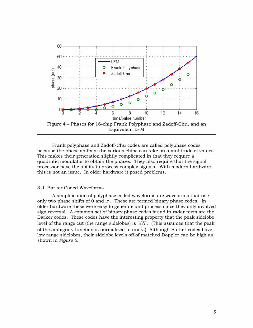
PRN waveforms most often have lengths of 2 1MN where M is an

integer. The sequence of phase shifts is determined by a feedback shift register device similar to that shown in Figure 6. In that figure the boxes represent binary shift register elements (flip-flops) and the adder is a modulo-2 adder. The characteristics of the sequence of ones and zeros produced by the feedback shift register are determined by which shift register stages are summed and fed back to the left-most shift register stage. Ideally, we want to choose the stages

so that the sequence of ones and zeros repeats only after 2 1MN samples,

where M is the number of stages in the shift register. Such a sequence of ones and zeros is termed a maximal length PRN sequence.

Skolnik2 has, on page 10.20, a tabulation of feedback configurations needed to generate maximal length sequences with lengths up to 220-1. The table contains only one feedback configuration for each code length. However, it indicates that there are generally several to many feedback configurations for each length. There are texts and web-sites that provide other feedback configurations. When searching for these you might use keywords such as “maximal length sequences” “shift register sequences”, “linear shift register sequences” and “pseudo random noise”. To generate a PRN sequence, one must initially load the shift register with any binary number except zero.

2 Skolnik, M. I., “Radar Handbook – Second Edition”, McGraw-Hill, New York, N.Y., 1990.

Figure 6 – M-stage Feedback Shift Register

8

Figure 7 contains a plot of the ambiguity function for a 15-chip PRN waveform where the phase coding was generated with the feedback configuration from your text and an initial load of 0001. It will be noted that the range cut doesn’t have sidelobes that are as low as for the Frank polyphase or Barker waverorms. However, the ambiguity function doesn’t have the large peaks that the other two waveforms exhibit. This is a characteristic of PRN coded waveforms: their sidelobe levels are generally “okay” but not extremely low or high. Long PRN coded waveforms have ambiguity functions that approach the ideal, “thumbtack” ambiguity function.

We noted above that we generated the phase code by using an initial load of 0001. It turns out that the initial load can have a fairly significant impact on the matched-Doppler range sidelobes of the ambiguity function. It also has a lesser impact on the other range-Doppler sidelobes. The only known way to

choose an initial load that provides the desired sidelobe characteristics is to experiment. As a side note: changing the initial load results in a phase coding sequence that is a cyclic shift of the original sequence. This is a property of maximal length PRN codes: they are periodic with a period of 2M-1.

Figure 7 – Ambiguity Function of a 15-chip PRN Coded Waveform

9

3.6 Mismatched PRN Processing

We now want to investigate a special type of processing of PRN coded waveforms that takes advantage of an interesting property of PRN codes. The property we refer to is that the circular autocorrelation of a PRN coded sequence has a value of either N or -1. With a circular correlation, when we shift the sequence to the right by n chips we take the n chps that “fall off” of the end of the shifted sequence and place them at the beginning of the shifted sequence. This is illustrated in Figure 8. In this figure we have used the 7-bi PRN code of 1001110 to generate the PRN coded sequence of -111-1-1-11.

To perform the circular autocorrelation we make a copy of the sequence to produce two sequences. We then circularly shift one sequence by n chips, multiply the result in N chip pairs and form a sum across the N chip result. This is illustrated in Figure 9. Mathematically we can write the circular correlation as

1

0N

N

n n kn

R k r r

(8)

where N

m denotes evaluation of m modulo N . The interesting property of

PRN coded sequences referenced above is that

0, ,2 ,

1 otherwise

N k N NR k

. (9)

Figure 8 – Illustration of a 2-bit Circular Shift

10

We now want to apply this property to examine a special type of PRN coded waveforms. We will assume that we encode a 0 of the PRN code to a

phase of 0 and a 1 of the PRN code to a phase shift of . Thus a single PRN

coded pulse corresponding to the 7-bit PRN code of Figures 8 and 9 would be as shown in Figure 10.

We assume that the transmit waveform, u t , is as shown in Figure 10.

We define a matched filter that is matched to a signal v t where v t is a

concatenation of three u t ’s. Thus v t would be as shown in Figure 11. The

0t reference points in Figures 10 and 11 are used to denote the time

alignment for matched range. Thus, when the received signal (a scaled version of Figure 10) is aligned with the center of the three PRN coded pulses of Figure 11 the matched filter is matched in range to the received pulse.

Figure 9 – Illustration of Circular Convolution for k=2.

Figure 10 – 7-chip, PRN Coded Waveform

Figure 11 – Waveform to which Matched Filter is Matched

11

The matched filter output, which is also the range cut of the cross

ambiguity function of u t and v t , is

2

0

0

, j ft

MF f

f

v u t h t dt f u t v t e dt

. (10)

We want to examine MFv for pn where p is the chip width and n is an

integer between 1N and 1N . We particularly want to examine the form

of pu t v t n . This is illustrated in Figure 12 for the aforementioned 7-chip

PRN coded waveform and 2n .

When we form 2 pu t v t we get

2

1

0

2 rectk

k N

Nj pj

p

k p

t ku t v t e e

(11)

and

22

1 1

0 0

2 rectk kk Nk N

N Njj pj

MF p p

k kp

t kv e e dt e

. (12)

We note from Figure 12 that 2N

k k

is equal to either 0 , or . We note

further that there are 3 cases where 20

Nk k

, 2 cases where 2

Nk k

and 2 cases where 2N

k k

. With this we get

02 3 2 2 3 4cosj j j

MF pv e e e . (13)

It turns out that for all 1p pN

3 4cosMFv . (14)

Figure 12 – Formation of 2 pu t v t

12

In fact, for any N-chip (N=2M-1) PRN coded waveform with u t and v t chosen

by the above rule,

1 1

cos 12 2

MF p p

N Nv N

. (15)

Stated in words, the range sidelobes within N-1 chips of the mainlobe have a constant value as given by Equation (15).

As an interesting extension of the above, if we choose such that

1 1cos 0

2 2

N N

(16)

or

1 1cos

1

N

N

(17)

we get

0 1MF p pv N . (18)

In words, the range sidelobes within N-1 chips of the mainlobe are zero. This has the potential of being useful in the situation a radar must be able to detect a very small target in the presence of a very large target, provided both targets are at the same Doppler.

Figure 13 contains a plot of the ambiguity function for the 7-chip PRN

example above. In the case the phase, , was chosen to be

1 11 7cos cos 0.75 138.59

1 7

. (19)

13

It will be noted that the range sidelobes around the central peak are, indeed, zero. However, it will be noted that the sidelobes off of matched Doppler rise significantly. It will also be noted that the range cut contains two extra peaks. These peaks are termed range ambiguities and are due to the fact that

u t correlates with each of the other two PRN coded pulses that make-up v t .

The range sidelobes adjacent to these range ambiguities are the normal range sidelobes associated with PRN coded waveforms.

3.7 Complementary Coded Pulses

The reference in footnote 1 contains a discussion of complementary pulses, or waveforms using complementary coded chips. These waveforms are

not PRN-based but also exhibit zero range sidelobes around the central peak. A binary, complementary coded waveform is illustrated in Figure 14 and its ambiguity function is illustrated in Figure 15. As noted with the PRN-coded waveform, the range sidelobes around the central peak are zero. However, the sidelobes off of matched Doppler are fairly large. The region of zero sidelobe level can be extended by extending the duration of the zero part of the waveform of Figure 14.

Figure 13 – Ambiguity Function for 7-chip Example Above

14

Complementary coded waveforms derive their name from the fact that

the components that makeup the waveform have range sidelobe levels that are negatives of each other. For example, the range sidelobes of the left-hand, four-pulse waveform of Figure 14 are the negative of the sidelobes of the right-hand four-pulse waveform. The fact that the waveforms are combined into a single waveform, with a dead space equal to at least the duration of each waveform, causes the sidelobes of one to add to the sidelobes of the other. Since the sidelobes have opposite signs, their sum is zero.

Figure 14 – Example of a Complementary Coded Waveform

Figure 15 – Ambiguity Function of the Complementary Coded Waveform of

Figure 14

15

3.8 Generation and Processing of Phase Coded Waveforms

To conclude our discussion of phase coded waveforms, we want to discuss, at least conceptually, how such waveforms are generated and how a matched filter might be implemented. Figure 16 contains a block diagram of a method that might be used to generate a phase coded waveform with arbitrary phase shifts on each pulse. The IF Oscillator generates quadrature signals at some intermediate frequency. The output of the synchronizer consists of two sequences of pulses where one sequence has amplitudes that depend upon the cosine of the phases on the individual pulses and the other sequence has amplitudes that depend upon the sine of the phases on the individual pulses.

For the case of the complimentary coded waveform of Figure 14, the cos k

would appear as shown in Figure 14 and the sin k output would be zero. If the

phases of the were other than 0 and the sin k output would be non-zero.

The left two mixers of Figure 16 are termed baseband mixers and, for all

practical purposes, are multipliers. The output of the top mixer is cos cosk IFt

and the output of the bottom mixer is sin sink IFt . The output of the summer

is

cos cos sin sin cosk IF k IF IF kt t t . (20)

As can be seen from Equation (20), the combination of the IF oscillator, synchronizer, two mixers and summer produce an IF signal that has the proper phase modulation imposed upon it.

The right mixer is a single-sideband mixer that produces the carrier signal with the proper phase modulation.

Figure 16 – Signal Generator for Phase Coded Waveforms

16

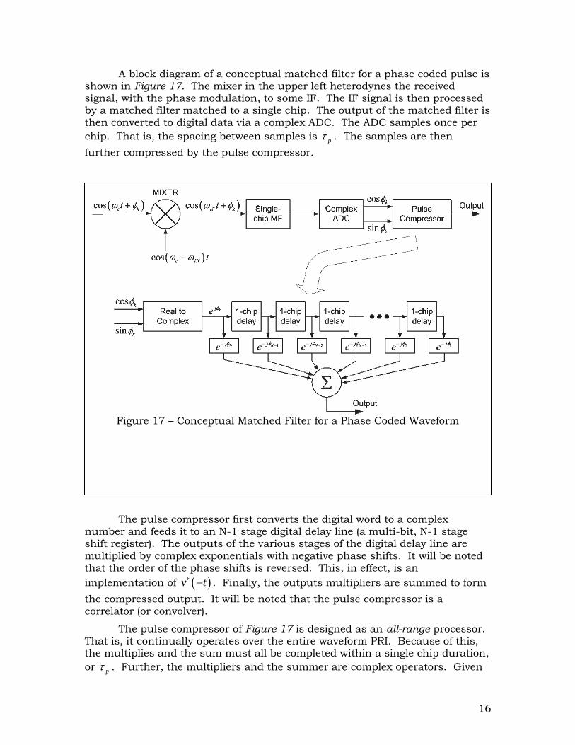
A block diagram of a conceptual matched filter for a phase coded pulse is shown in Figure 17. The mixer in the upper left heterodynes the received signal, with the phase modulation, to some IF. The IF signal is then processed by a matched filter matched to a single chip. The output of the matched filter is then converted to digital data via a complex ADC. The ADC samples once per

chip. That is, the spacing between samples is p . The samples are then

further compressed by the pulse compressor.

The pulse compressor first converts the digital word to a complex number and feeds it to an N-1 stage digital delay line (a multi-bit, N-1 stage shift register). The outputs of the various stages of the digital delay line are multiplied by complex exponentials with negative phase shifts. It will be noted

that the order of the phase shifts is reversed. This, in effect, is an

implementation of v t . Finally, the outputs multipliers are summed to form

the compressed output. It will be noted that the pulse compressor is a correlator (or convolver).

The pulse compressor of Figure 17 is designed as an all-range processor. That is, it continually operates over the entire waveform PRI. Because of this, the multiplies and the sum must all be completed within a single chip duration,

or p . Further, the multipliers and the summer are complex operators. Given

Figure 17 – Conceptual Matched Filter for a Phase Coded Waveform

17

this, very high speed digital hardware is needed to process phase coded waveforms of even moderate bandwidth.

The processing load can be relieved if the waveform is used over only a limited range window. In this case, the correlator in the bottom part of Figure 17 would be replaced with a combination of an FFT, a complex, vector multiplier, and an inverse FFT. The length of the FFT, multiplier and inverse FFT would depend upon the size of the range window, in chips and the number

of chips in the phase coded waveform. Specifically, if the range window is RWN

chips long and the phases coded waveform contains N chips, or subpulses,

then the minimum FFT length would be

2FFT RWN N N . (21)

The factor of 2N is needed to account for the fact that the output of the

matched filter is two times longer than the overall pulse width.

As an example, suppose one wanted to process a range window of 15 Km and was using a phase coded waveform with a bandwidth of 10 MHz and a duration of 10 µs. The 10 MHz bandwidth translates to a chip width of 0.1 µs,

or 15 m. With this we get

15000 15 1000RWN (22)

and

10 s100

0.1 sN

. (23)

From these two values we get

2 2 100 1000 1200FFT RWN N N . (24)

This means that the pulse compressor will require a 2048 point FFT and IFFT, and will require 2048 complex multiplies. The combination of the FFT, IFFT and multiply would need to be completed in one PRI. If one uses a PRI of say, 500 µs, then the operations would need to be completed in 500 µs. This is still

stressing but may be easier than the all-range implementation of Figure 17. In some applications where latency is not a major issue, the FFT, multiply and IFFT operations can be pipelined to ease computing requirements. In such an application the FFT would be performed on one PRI, the multiply on the next PRI and the IFFT on the third PRI. Further, while the IFFT is being performed on the Kth pulse, the multiply would be performed on the (K+1)th pulse and the FFT would be performed on the (K+2)th pulse.

If the phase coding is restricted to binary, with phase shifts of 0 and , rather than polyphase, the generation and processing of the phase coded waveforms becomes considerably simpler. In Figure 16 the sine channel can be eliminated and in the pulse compressor the arithmetic becomes real instead of complex. In some instances the arithmetic is further simplified to single-bit arithmetic.

18

3.9 Step Frequency Waveforms

3.9.1 The Basics

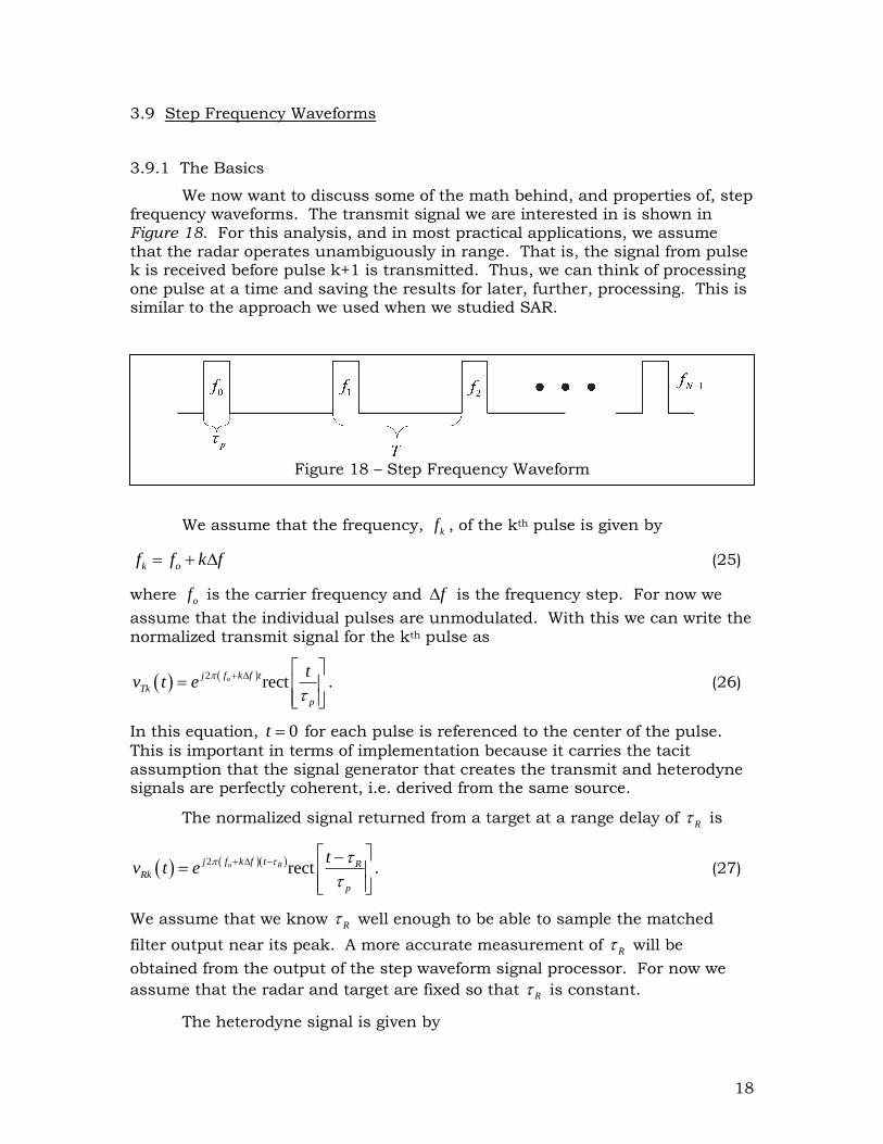
We now want to discuss some of the math behind, and properties of, step frequency waveforms. The transmit signal we are interested in is shown in Figure 18. For this analysis, and in most practical applications, we assume that the radar operates unambiguously in range. That is, the signal from pulse k is received before pulse k+1 is transmitted. Thus, we can think of processing one pulse at a time and saving the results for later, further, processing. This is similar to the approach we used when we studied SAR.

We assume that the frequency, kf , of the kth pulse is given by

k of f k f (25)

where of is the carrier frequency and f is the frequency step. For now we

assume that the individual pulses are unmodulated. With this we can write the normalized transmit signal for the kth pulse as

2rectoj f k f t

Tk

p

tv t e

. (26)

In this equation, 0t for each pulse is referenced to the center of the pulse.

This is important in terms of implementation because it carries the tacit assumption that the signal generator that creates the transmit and heterodyne signals are perfectly coherent, i.e. derived from the same source.

The normalized signal returned from a target at a range delay of R is

2recto Rj f k f t R

Rk

p

tv t e

. (27)

We assume that we know R well enough to be able to sample the matched

filter output near its peak. A more accurate measurement of R will be

obtained from the output of the step waveform signal processor. For now we

assume that the radar and target are fixed so that R is constant.

The heterodyne signal is given by

Figure 18 – Step Frequency Waveform

19

2 oj f k f t

kh t e

. (28)

We note that the frequency of the heterodyne signal is different for every pulse

and that kh t is perfectly coherent with Tkv t . With this, the output of the

heterodyne operation is

2 2 recto R Rj f j f RHk Rk k

p

tv t v t h t e e

. (29)

The first term is a constant phase shift that will be common to all pulses. We will lump it into some constant that we will drop.

For the next step we pass Hkv t through a matched filter matched to

rectp

t

to produce a normalized output of

2 triRj k f RMk

p

tv t e

(30)

where tri x is a triangle centered at 0x with a base width of 2 and a height

of unity.

Finally, we sample Mkv t at some , close to R , to obtain

2 triRj k f RMk

p

v e

. (31)

After we obtain Mkv from N pulses we form the sum

1 1

2

0 0

tri R

N Nj k fR

R k Mk k

k kp

V a v a e

(32)

where the ka are complex weight coefficients that we choose to maximize

RV . We recognize Equation (32) as the form of the sum we have

encountered in our antenna, stretch processing and SAR analyses. We can use

this knowledge to postulate a form of the ka as

2j k f

ka e (33)

and write RV as

1

2

0

tri R

Nj k fR

R k

kp

V a e

(34)

We can evaluate and normalize Equation 34 to yield

20

sintri

sin

RRR

p R

N fV

f

. (35)

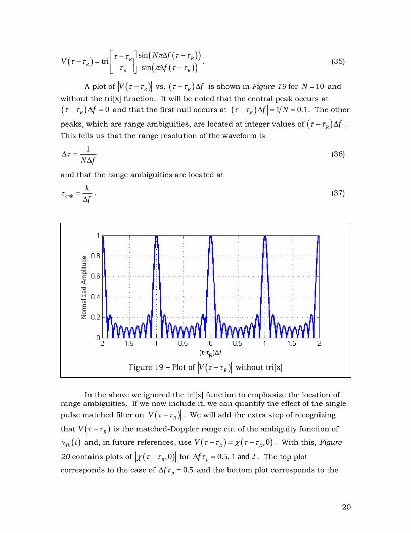
A plot of RV vs. R f is shown in Figure 19 for 10N and

without the tri[x] function. It will be noted that the central peak occurs at

0R f and that the first null occurs at 1 0.1R f N . The other

peaks, which are range ambiguities, are located at integer values of R f .

This tells us that the range resolution of the waveform is

1

N f

(36)

and that the range ambiguities are located at

amb

k

f

. (37)

In the above we ignored the tri[x] function to emphasize the location of range ambiguities. If we now include it, we can quantify the effect of the single-

pulse matched filter on RV . We will add the extra step of recognizing

that RV is the matched-Doppler range cut of the ambiguity function of

Tkv t and, in future references, use ,0R RV . With this, Figure

20 contains plots of ,0R for 0.5, 1 and 2pf . The top plot

corresponds to the case of 0.5pf and the bottom plot corresponds to the

Figure 19 – Plot of RV without tri[x]

21

case of 2pf . The dashed triangles are the single-pulsed matched filter

responses.

It will be noted that for 0.5 and 1pf the single-pulse matched filter

response attenuates the range ambiguities. However, when 2pf the range

ambiguities are present. This interaction of the single-pulse matched filter response is a limitation that must be considered when designing step frequency

waveforms. Specifically, if one increases f in an attempt to improve range

resolution one runs the risk of introducing range ambiguities. From this we see

that, for a given N there is direct relation between f and the width of the

individual pulses. To improve resolution by increasing f , and avoid range

ambiguities, we must assure that

1pf . (38)

It turns out that a means of effectively reducing p is to use a pulse

compression waveform on the individual pulses. In that case p would be the

compressed pulse width. Another means of improving range resolution would be to increase the number of pulses that are processed. However, this must be done with care in that it can have negative consequences in terms of timelines and the potential impact of target motion.

Figure 20 – Plot of ,0R for 0.5, 1 and 2pf

22

3.9.2 Doppler Effects

We now want to consider the effects of target motion. For now we will be concerned with only target Doppler. To include target Doppler, we write the target range as

0R t R Rt (39)

and the target range delay as

0 02R R R d ot R c t f f t . (40)

We can write the target range delay at the time of the kth transmit pulse as

0R Rk R d okT f f kT (41)

where T is the PRI (see Figure 18).

If the transmit signal defined in Equation (26) then the received signal is

0

2

2

rect

rect

o Rk

o R d o

j f k f t RkRk

p

j f k f t f f kT Rk

p

tv t e

te

. (42)

If we manipulate the above using o d o df k f f f f with 0Rk R in the

rect[x] function we get

02 2 2 0recto R dj f k f t j k f j f kT RRk

p

tv t e e e

. (43)

We note that the approximation of o d o df k f f f f may not be very good.

However, it allows us to focus directly on the effects of target Doppler and not be concerned with the potential smearing effects the approximation could cause. This would need to be considered in a more complete analysis.

If we compare Equation 43 with Equation (27) we note that the only difference is the appearance of the term related to Doppler. Thus, if we repeated the heterodyning and matched filtering math from above we would get

02 2 00 triR dj k f j f kT R

Mk R

p

v e e

. (44)

If we form a weighted sum of the 0Mk Rv as we did before we would get

0

1 12 0

0

0 0

triR d

N Nj f f T k R

R Mk k

k k p

V v b e

. (45)

23

As we did earlier, we want to choose the kb to maximize 0RV . However, a

more general form would be to use

2j f fT k

kb e

(46)

which would yield

0

120

0

0

, tri R d

Nj f f f T kR

R d

kp

f f e

(47)

Or, evaluating the sum,

000

0

sin, tri

sin

R dRR d

p R d

N f f f Tf f

f f f T

. (48)

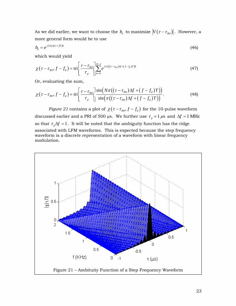
Figure 21 contains a plot of 0,R df f for the 10-pulse waveform

discussed earlier and a PRI of 500 µs. We further use 1 sp and 1 MHzf

so that 1p f . It will be noted that the ambiguity function has the ridge

associated with LFM waveforms. This is expected because the step frequency waveform is a discrete representation of a waveform with linear frequency modulation.

Figure 21 – Ambituity Function of a Step Frequency Waveform

24

Figure 22 contains a matched-range, Doppler cut plot, a plot of

0, df f vs. df f , of the step frequency waveform. It will be noted that the

Doppler resolution of this waveform is 20 KHz or 1 NT , as expected.

Figure 23 contains plots of range cuts at matched Doppler and at a Doppler offset of one Doppler resolution cell (200 Hz). It will be noted that a Doppler offset of one Doppler resolution cell causes a range error of one range resolution cell. This means that the step frequency waveform is very sensitive to Doppler and that, if we want accurate absolute range measurement, the range shift due to target Doppler must be removed. This can be done if the target is in track and the relative velocity between the radar and target is known with reasonable accuracy.

If the step frequency waveform is used in its more common role of target imaging (or SAR), the various scatterers of the target should be moving at about the same range-rate so that range errors due to Doppler differences of the scatterers should be small. One would still want to remove the gross Doppler so as to minimize losses due to Doppler mismatch. (It will be noted from Figure

23 that the range cut at 1f NT is down about 1 dB (-10log(0.9).)

Figure 22 – Matched-Range, Doppler Cut for a Step Frequency Waveform

25

Figure 23 – Range Cuts of a Step Frequency Waveform