Seventh Framework Programme Theme 6 Environment Collaborative Project (Large-scale Integrating Project) Project no. 212085 Project acronym: MEECE Project title: Marine Ecosystem Evolution in a Changing Environment D1.4 New model parameterisations Part B: Metabolic Theory Due date of deliverable: 31.08.2010 Actual submission date: 31.08.2011 Organisation name of lead contractor for this deliverable: UHAM Start date of project: 01.09.08 Duration: 48 months Project Coordinator: Icarus Allen, Plymouth Marine Laboratory Project co-funded by the European Commission within the Seventh Framework Programme, Theme 6 Environment Dissemination Level PU Public x PP Restricted to other programme participants (including the Commission) RE Restricted to a group specified by the consortium (including the Commission) CO Confidential, only for members of the consortium (including the Commission)

Welcome message from author
This document is posted to help you gain knowledge. Please leave a comment to let me know what you think about it! Share it to your friends and learn new things together.
Transcript
Seventh Framework Programme Theme 6 Environment
Collaborative Project (Large-scale Integrating Project)
Project no. 212085
Project acronym: MEECE
Project title: Marine Ecosystem Evolution in a Changing Environment
D1.4 New model parameterisations
Part B: Metabolic Theory
Due date of deliverable: 31.08.2010
Actual submission date: 31.08.2011
Organisation name of lead contractor for this deliverable: UHAM
Start date of project: 01.09.08 Duration: 48 months Project Coordinator: Icarus Allen, Plymouth Marine Laboratory
Project co-funded by the European Commission within the Seventh Framework Programme,
Theme 6 Environment
Dissemination Level
PU Public x
PP Restricted to other programme participants (including the Commission)
RE Restricted to a group specified by the consortium (including the Commission)
CO Confidential, only for members of the consortium (including the Commission)

EC FP7 MEECE | 212085 | D1.4 | New model parameterisations, Part B: Metabolic Theory
Page 1 of 42
D1.4 Meta analysis of the driver databases and development of new parameterisations relevant to the ecosystem models
Part B: Metabolic Theory
Main Contributor: IEO
Contents
1. Introduction ................................................................................................................. 3
2. Temperature dependence of Metabolic rates ............................................................... 3
2.1 From single molecules to biochemical kinetics. ................................................... 3
2.2. From biochemical kinetics to whole organism physiology. ................................. 3
2.3 From organisms to communities, biogeochemical cycles and biodiversity. ......... 4
2.4 References ......................................................................................................... 4
3. Temperature-Abundance-Size relationships in marine plankton ............................ 5
3.1. Summary ........................................................................................................... 5
3.2. Methodology ...................................................................................................... 6
3.3. Results .............................................................................................................. 6
3.4. References ...................................................................................................... 14
4. Temperature, nutrients and the size-scaling of phytoplankton growth in the sea .. 16
4.1. Summary ......................................................................................................... 17
4.2. Methods ........................................................................................................... 17
4.3. Results ............................................................................................................ 17
4.4. References ...................................................................................................... 21
5. The evolution of high prey capture rates in planktivorous fish and jellyfish ........... 22
5.1. Summary ......................................................................................................... 22
5.2 Methods ............................................................................................................ 22
5.3 Results ............................................................................................................. 22
6. A unified model of life history optimization and metabolic scaling theories for developmental time ................................................................................................... 24
6.1. Summary ......................................................................................................... 24
6.2 The model........................................................................................................ 25
EC FP7 MEECE | 212085 | D1.4 | New model parameterisations, Part B: Metabolic Theory
Page 2 of 42
6.2.1 The MTE approach............................................................................. 25
6.2.2 LHO trade-offs ................................................................................... 27
6.2.3 An ensembled model of MTE and LHO ............................................. 27
6.3 Materials and methods..................................................................................... 28
6.4 Results ............................................................................................................ 28
6.4.1 MTE model: allometric, growth efficiency and size increment effects 28
6.4.2 The Offspring-Size/Clutch-Size ......................................................... 31
6.4.3 Combined effects of LHO and MTE on developmental time .............. 31
6.5 Discussion ....................................................................................................... 32
6.6 References ....................................................................................................... 35
6.7. Supplementary Material. .................................................................................. 37
EC FP7 MEECE | 212085 | D1.4 | New model parameterisations, Part B: Metabolic Theory
Page 3 of 42
Meta Analysis: Metabolic Theory
1. Introduction
The aim of this task was the use of metabolic theory building on pervious work using metabolic theory of ecology (MTE) (Allen et al., 2005) in marine system (Lopez Urrutia et al 2006) to further develop a synthetic theory to explain the effects of body size, temperature and resources on the metabolism of the oceans going from organism to population and communities to whole ecosystems. The objective was to develop a theory that enables us to explain and model the effects of changing light levels, temperature, stoichiometry, size structure on planktonic metabolism. The challenge is then to extend the patterns depicted at the organism level to ecosystem properties relevant for global processes like export production, species diversity and population abundance.
2. Temperature dependence of metabolic rates
2.1. From single molecules to biochemical kinetics.
Temperature affects the velocity of biochemical reactions which drive organism metabolism. Statistical thermodynamics is in essence a macroscopic rule used to predict the effects of temperature on chemical reactions. In an ideal gas at thermal equilibrium, it is impossible to describe the kinetic energy associated with each individual molecule, but Maxwell-Boltzmann distribution law shows that the probability of a molecule occupying a kinetic energy E is proportional to where k is Boltzmann constant (8.62*10-5 eV K-1) and T the system's absolute temperature (K). There is an interesting resemblance between what this law represented (a bridge between microscopic physicists interested in single molecule dynamics and macroscopic physicists interested in whole systems dynamics) and the aim of macroecology as a discipline linking ecophysiology and community ecology. Implicit in Maxwell-Boltzmann equation is the fact that as temperature increases the proportion of molecules with sufficient kinetic energy to react increases. This ultimately led Svante Arrhenius to formulate that the temperature dependence of reaction kinetics should scale as where R is the gas constant (8.31 J mol−1 K−1) and Ea is the activation energy of that particular reaction; reactions with higher Ea show stronger temperature dependence. The difference between Boltzmann's factor and Van't Hoff-Arrehnius equation is just that the former uses particle units (E in eV and k in eV K-1) while the latter uses the molar scale (Ea in J mol-1 and R in J mol−1 K−1). Because k and R are related by k=R/(NA*j), where NA is Avogadro constant (NA=6.022 *1023) and a j conversion factor from electronvolts to Joules (j=1.602 *10-19 J eV -1 ), both expressions have the same value. The more intuitive Q10 constant results from simplification of Van't Hoff-Arrehnius equation (Gillooly et al. 2002).
2.2. From biochemical kinetics to whole organism physiology.
A second scaling step is needed to apply Boltzmann's – Arrhenius equation to the response of whole organism physiological rates to temperature. Although Boltzmann's – Arrhenius equation has been widely applied to biological systems, just recently the activation energy measured for whole-organism rates has been related to the activation energy of the main biochemical reactions that drive organism physiology (Gillooly et al. 2001). Metabolic scaling theory proposes that because organism metabolism is mainly driven by mitochondrial respiration, the temperature dependence of adenosine triphosphate (ATP) synthesis should determine the temperature dependence of whole-organism metabolic rate with an average activation energy for both processes close to 0.65 eV (or 62.7 KJ mol-1) (Gillooly et al 2001). Although whole-organisms greatly depart from the ideal gas conditions for which Boltzmann's –

EC FP7 MEECE | 212085 | D1.4 | New model parameterisations, Part B: Metabolic Theory
Page 4 of 42
Arrhenius equation was formulated and more complex explanations have emerged (Clarke 2004) the similar activation energy at both levels of organization is quite remarkable. For planktonic heterotrophs, whose metabolism is mainly driven by the synthesis of ATP, the activation energy for both respiratory (Lopez-Urrutia et al 2006) and growth rates (Rose and Caron 2007) is close to the predicted value of 0.65 eV. But the temperature dependence of the metabolic rates of photosynthetic plankton has long been recognized to be lower than that of heterotrophs (Eppley 1972) with values ranging from 0.29 to 0.39 eV (Lopez-Urrutia et al 2006, Rose and Caron 2008). Allen et al (2005) argued that the lower temperature dependence of land-plant photosynthetic rates (0.32 eV) is due to the kinetics of rubisco carboxylation and photorespiration. As temperature increases photorespiration increases relative to carboxylation thus reducing net carbon gain. The applicability of Allen et al (2005) explanation to marine plankton depends on the assumption that CO2 supply to Rubisco in marine plants, which have different diffusive characteristics and carbon concentration mechanism (Yvon-Durocher et al 2010), does not modify this theoretical explanation.
2.3 From organisms to communities, biogeochemical cycles and biodiversity.
Regardless of the theoretical basis for the differential temperature dependence of the metabolic and growth rates of autotrophs and heterotrophs, the implication for to marine plankton community dynamics and biogeochemical cycles are far reaching. Huntley and Boyd (1984) showed that the zooplankton to phytoplankton production ratio would increase as temperature increases. Rose and Caron (2007) argued that phytoplankton blooms might occur more frequently in cold waters because the growth of grazers will be much lower than the growth of phytoplankton as temperature decreases. Laws et al. (2000) showed that the proportion of primary production exported to the deep increases with decreasing temperature because, at cold temperatures, the growth rates of heterotrophic decomposers are much lower so most organic matter is exported before it can be decomposed. Lopez-Urrutia et al (2006) scaled the differential temperature dependence of planktonic respiration and photosynthesis to the metabolic balance of whole plankton communities and showed that as temperature increases the ratio of community production to respiration decreases. Through its effects on organism metabolic rates, temperature also affects community structure. Higher cell division rates with increasing temperature might be responsible for the stronger DNA evolution and speciation rates observed in planktonic foraminifera towards the tropics (Allen and Gillooly 2006). This kinetic energy hypothesis plays a fundamental role on the observed temperature dependent global patterns of marine biodiversity both in planktonic and other marine communities (Tittensor et al 2010).
2.4 References
Allen AP, Gillooly JF, Brown JH (2005) Linking the global carbon cycle to individual metabolism. Funct Ecol 19:202–213.
Allen AP, Gillooly JF (2006) Assessing latitudinal gradients in speciation rates and biodiversity at the global scale. Ecol Lett 9:947–954.
Eppley R (1972) Temperature and phytoplankton growth in the sea. Fish Bull (Seattle) 70:1063–1085.
Huntley M, Boyd C (1984) Food-limited growth of marine zooplankton. Am Nat 124:455–478.
Gillooly JF, Brown JH, West GB, Savage VM, Charnov EL (2001) Effects of size and temperature on metabolic rate. Science 293:2248–2251.
Gillooly JF, Charnov EL, West GB, Savage VM, Brown JH (2002) Effects of size and temperature on developmental time. Nature 417:70–73
EC FP7 MEECE | 212085 | D1.4 | New model parameterisations, Part B: Metabolic Theory
Page 5 of 42
Laws EA, Falkowski PG, Smith Jr WO, Ducklow H, McCarthy JJ (2000) Temperature effects on export production in the ocean. Glob Biogeoch Cycles 14:1231–1246.
Rose J, Caron D (2007) Does low temperature constrain the growth rates of heterotrophic protists? Evidence and implications for algal blooms in cold waters. Limnol Oceanogr 52:886–895.
Tittensor DP, Mora C, Jetz W, Lotze HK, Ricard D, Berghe EV, Worm B (2010) Global patterns and predictors of marine biodiversity across taxa. Nature 466:1098–1101.
Yvon-Durocher, G., Allen, A.P., Montoya, J.M., Trimmer, M. and Woodward, G. (2010) The temperature dependence of the carbon cycle in aquatic systems. Advances in Ecological Research, 43, in press.
3. Temperature-Abundance-Size relationships in marine plankton
3.1. Summary
Picophytoplankton are photosynthetic unicellular organisms in the 0.2-2 µm size range that are found throughout the world’s oceans. They comprise cyanobacteria of the genera Synechococcus and Prochlorococcus (Partensky et al., 1999) together with a diverse ensemble of eukaryotic algae (Moon-van der Staay et al., 2001, Notet al., 2007). Picophytoplankton cells have a ubiquitous distribution and contribute significant portions of bulk phytoplankton biomass and production (Bell et al., 2001, Agawinet al., 2000). The accepted view poses them as the dominant primary producers in vast areas of oligotrophic oceans although they may also become important in coastal seas (Morán, 2007). The structure and functioning of planktonic communities is strongly dependent on the relative importance of picophytoplankton, directly impacting the ecosystem balance of organic carbon produced in the upocean (Legendre et al., 1991, Falkowski et al., 1998). A recent study has demonstrated that some of the carbon produced by picophytoplankton may also be exported to the deep ocean (Richardson et al., 2007). The effects of temperature on the biomass and production of phytoplankton assemblages in the context of global ocean warming have been addressed in several studies (Richardson et al., 2004, Li et al., 2006, Bopp et al., 2001, Behrenfeld et al., 2006), but seldom focused specifically on the smallest size-class. In the review by Agawin et al (2000), temperature was positively related with the relative contribution of small cells to total primary production but not to total chlorophyll, showing that chlorophyll may not be as good a proxy for biomass in the picoplankton size class. A remarkably coherent pattern of total phytoplankton cell density increase with temperature was found in the temperate NW Atlantic by (Li et al., 2006). The overwhelmingly dominant contribution of picophytoplankton to total cell abundance is (Li, 2002) implicitly suggests that some universal underlying mechanism may apply for both large and small phytoplankton. Although ongoing climate warming has been shown to result in a decline of total phytoplankton biomass, especially in subtropical oligotrophic regions (Richardson et al., 2004, Behrenfeld et al., 2006)), we lack a theoretical explanation for the unexpected parallel increase in absolute cell abundance (Li et al. 2006). We combine here two large time-series datasets of picophytoplankton abundance, cell size and biomass collected in mostly temperate North Atlantic waters, and apply current theories of temperature-size relationships and the allometric size-scaling of population abundance to explain remarkably consistent relationships between temperature and the biomass of primary producers across the eastern and western shores. This analysis provides a theoretical framework for assessing how marine phytoplankton communities might change in the near future.
EC FP7 MEECE | 212085 | D1.4 | New model parameterisations, Part B: Metabolic Theory
Page 6 of 42
3.2. Methodology Data were obtained in different cruises carried out from 1994 to 2005 in the NW Atlantic Ocean (42-60ºW, see Fig. S1 in {Li, 2006 #4017}) and during a 5-year period (Apr 2002- Mar 2007) within a long-term monitoring program with monthly samples in the NE (5ºW, see Fig. 1 in {Calvo-Díaz, 2008 #38 et al. 2007}). Latitude was 43ºN in the NE and although most data in the NW came from the same latitude, 39% of them were obtained at latitudes ranging from 54º to 60ºN. The seasonal cycle was well-covered by both datasets, with evenly distributed data in the NW but fewer winter data in the NE (~5% of the total). All data were obtained at the surface (NE, n=59) or the upper 10 m of the water column (NW, n=97). Selected environmental variables are shown in Table S1. Spatial autocorrelation was avoided by averaging results from 3 (NE) or more stations (NW) sampled during the same day. Seawater samples were collected from Niskin bottles and processed as detailed elsewhere (Li et al., 2006, Morán, 2007). Chlorophyll a concentration was measured fluorometrically in acetone extracts. Nutrient concentrations were determined with Technicon autoanalyzers. Picophytoplankton samples were fixed with paraformaldehyde 1% + glutaraldehyde 0.05% (NE) or paraformaldehyde 1% (NW) and stored frozen at -80ºC until analysis. Thawed samples were counted by flow cytometry (Li et al., 2006, Morán, 2007). The size of picophytoplankton cells was estimated from cytometric light scatter signals calibrated with microspheres (NW) or through sequential size fractionation of the community with Nuclepore polycarbonate filters (NE). Picophytoplankton biomass was estimated from abundance and cell size data for each dataset
using a common conversion factor of 237 fg C µm-3 (Worden et al., 2004) and a C:chlorophyll ratio (mg:mg) of 50 (Harris, 1986) was used for estimating total phytoplankton biomass from chlorophyll measurements. Although the C:chlorophyll ratio is dependent on factors such as taxonomic composition or irradiance, it is unlikely that these changes were different in both Atlantic sides so as to preclude the cross-regional comparison of total phytoplankton biomass intended in this study. All linear regressions were performed according to the ordinary least squares (OLS) method or Model I, since measurement errors in temperature are much lower than those corresponding to phytoplankton variables.
3.3. Results
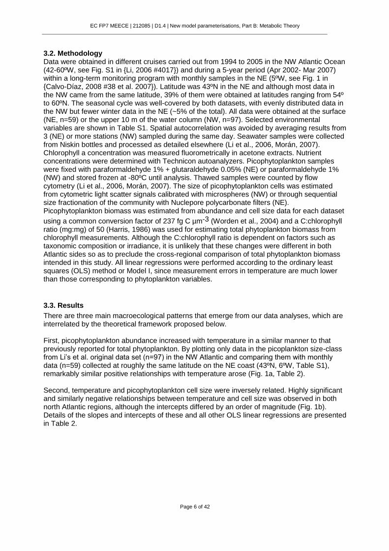
There are three main macroecological patterns that emerge from our data analyses, which are interrelated by the theoretical framework proposed below. First, picophytoplankton abundance increased with temperature in a similar manner to that previously reported for total phytoplankton. By plotting only data in the picoplankton size-class from Li’s et al. original data set (n=97) in the NW Atlantic and comparing them with monthly data (n=59) collected at roughly the same latitude on the NE coast (43ºN, 6ºW, Table S1), remarkably similar positive relationships with temperature arose (Fig. 1a, Table 2). Second, temperature and picophytoplankton cell size were inversely related. Highly significant and similarly negative relationships between temperature and cell size was observed in both north Atlantic regions, although the intercepts differed by an order of magnitude (Fig. 1b). Details of the slopes and intercepts of these and all other OLS linear regressions are presented in Table 2.
EC FP7 MEECE | 212085 | D1.4 | New model parameterisations, Part B: Metabolic Theory
Page 7 of 42
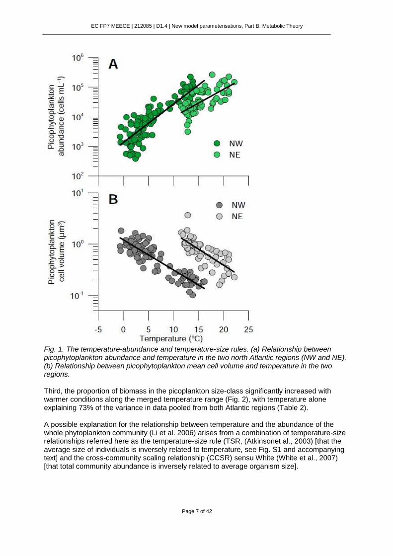
Fig. 1. The temperature-abundance and temperature-size rules. (a) Relationship between picophytoplankton abundance and temperature in the two north Atlantic regions (NW and NE). (b) Relationship between picophytoplankton mean cell volume and temperature in the two regions. Third, the proportion of biomass in the picoplankton size-class significantly increased with warmer conditions along the merged temperature range (Fig. 2), with temperature alone explaining 73% of the variance in data pooled from both Atlantic regions (Table 2). A possible explanation for the relationship between temperature and the abundance of the whole phytoplankton community (Li et al. 2006) arises from a combination of temperature-size relationships referred here as the temperature-size rule (TSR, (Atkinsonet al., 2003) [that the average size of individuals is inversely related to temperature, see Fig. S1 and accompanying text] and the cross-community scaling relationship (CCSR) sensu White (White et al., 2007) [that total community abundance is inversely related to average organism size].
EC FP7 MEECE | 212085 | D1.4 | New model parameterisations, Part B: Metabolic Theory
Page 8 of 42
Fig. 2. Increasing dominance of picophytoplankton biomass with temperature. Relationship between the percent contribution of picophytoplankton to total phytoplankton biomass and temperature in the two regions. Fitted line is OLS linear regression for pooled log-transformed data (see Table 2 for details). The relationships between organism size are temperature within and across taxa are of various types, of which the TSR is just one. Strictly speaking this rule applies to phenotypic plasticity, not to changes in average size in a population, as argued here, which can arise from selection against particular-sized genotypes as well as plasticity. Bergmann’s or James’ rule is another well-known temperature-size relationship used to describe an increase in the body size of a species as latitude increases or environmental temperature decreases, loosly applied to endotherms and ectotherms. Exceptions to the TSR rule are actively debated and out of the object of this analysis, but sometimes the same mechanism may be used to explain a reduction in maximum (and potentially mean) size in aquatic ectotherm taxa with reduced latitude (Makarieva et al. 2005). As a corollary of the TSR and CCSR theories, and under an energetic equivalence scenario (i.e. the same amount of resources utilized by all size classes) temperature should affect community abundance but indirectly through its effects on body size. In warmer conditions the average size of the organisms in a community would decrease as a consequence of the TSR (as shown in Fig. 1b for picophyplankton) and because smaller organisms have lower absolute energy requirements (Gillooly et al., 2001) the number of phytoplankton cells that can be sustained will be higher as shown by Li et al. (2006). For picophytoplankton our argument is a bit more complicated. If its contribution to total phytoplankton remains constant with temperature, then picophytoplankton abundance should increase with increasing temperature solely because total phytoplankton abundance increases (i.e. the same percentage of a larger number). However, we argue that the relative contribution of picophytoplankton to the total biomass of planktonic primary producers should vary with temperature as a consequence of a combination of the TSR and the within-community size scaling of abundance or individual size distribution (ISD) (White et al., 2007), that is, the frequency distribution of individual body sizes in a community. Note that the ISD is distinct from the CCSR mentioned above for total phytoplankton.
EC FP7 MEECE | 212085 | D1.4 | New model parameterisations, Part B: Metabolic Theory
Page 9 of 42
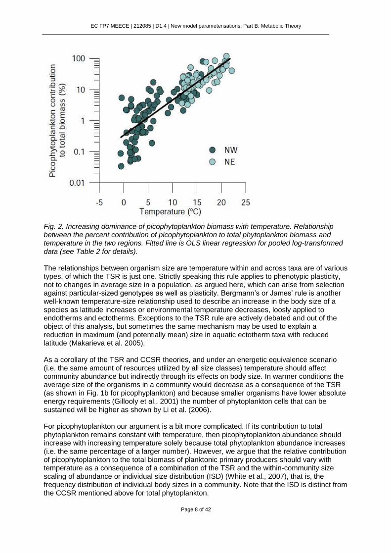
Fig. 3. Schematic representation of the effects of temperature on the size-scaling of phytoplankton abundance. (a) and (b) represent idealized individual size distributions (ISD) of two different phytoplankton communities at 10 and 20ºC, respectively. At high temperatures (b) the mean cell size of the phytoplankton community is lower than at low temperatures (a) so the ISD is shifted upwards to the left. Hence a higher proportion of total cell abundance falls into the picoplankton (<2 µm) size-class under warmer conditions (hatched area). (c) The abundance-temperature relationship emerges when the picophytoplankton abundances from different communities such as those represented in (a) and (b) are plotted in a cross-community chart against temperature. S1 and S2 are mean picophytoplankton cell sizes at
10ºC and 20ºC, respectively, with corresponding abundances A1 and A2. S1>S2, A1<A2.
To explain the observed relationships between picophytoplankton abundance and temperature shown in Fig. 1a we show the hypothetical distribution of the abundance of all cells within the phytoplankton community versus size at two different temperatures (10º and 20ºC, Fig. 3). As discussed above an increase in temperature would shift the total community to smaller sizes. The average size and abundance of picophytoplankton at a given temperature for each station and sampling period would translate into a plot of picophytoplankton abundance versus temperature equivalent to that shown in Fig. 1a for data collected in the NW and NE Atlantic Ocean. Because the nominal upper size boundary of picoplankton is fixed at 2 µm (Sieburth et al., 1978), the ISD would be shifted towards smaller sizes as temperature rises (Fig. 3) and hence a larger proportion of the community will be smaller than that size.

EC FP7 MEECE | 212085 | D1.4 | New model parameterisations, Part B: Metabolic Theory
Page 10 of 42
Fig. 4. Opposite relationships of picophytoplankton and total phytoplankton biomass with temperature. (a) Relationship between picophytoplankton biomass and temperature in the two
regions. (b) Relationship between picophytoplankton biomass per µmol L-1 of phosphate (picophytoplankton biomass : PO4 ratio) and temperature in the two regions. (c) Relationship
between total phytoplankton biomass and temperature in the two regions. Fitted lines are OLS linear regressions for log-transformed pooled data (see Table 2 for details and individual data set regressions). Based on the conceptual framework depicted in Fig. 3, we could make two predictions. First, that there should exist a strong relationship between temperature and the contribution of picophytoplankton to total phytoplankton abundance and biomass. Second, that picophytoplankton abundance should be more related than total phytoplankton abundance to temperature (steeper slope), because the former is determined not only by the TSR – CCSR relationship but also by the TSR – ISD relationship. These predictions were supported by our datasets: a significant increase in the proportion of biomass in the picoplankton size-class with warmer conditions became evident for the entire temperature range (Fig. 2), with a remarkably high percentage of its variance explained by this single factor. Our results thus complement previous demonstrations of a significant increase in the proportion of picophytoplankton primary production with temperature (Agawin et al., 2000). According to our analysis, picophytoplankton would dominate the biomass of primary producers in the ocean’s surface at a temperature of 19.7ºC, although noticeable fractions would already be present at lower
EC FP7 MEECE | 212085 | D1.4 | New model parameterisations, Part B: Metabolic Theory
Page 11 of 42
temperatures. A rise in temperature of 3ºC would double picophytoplanktonic contribution at 15ºC (32% vs 15%). Also as predicted, the slope of the picophytoplankton abundance vs. temperature regression was 19% higher than that corresponding to total phytoplankton in the NE region (Table 2).
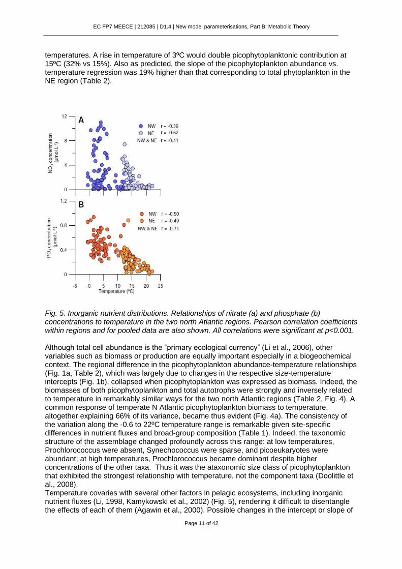
Fig. 5. Inorganic nutrient distributions. Relationships of nitrate (a) and phosphate (b) concentrations to temperature in the two north Atlantic regions. Pearson correlation coefficients within regions and for pooled data are also shown. All correlations were significant at p<0.001. Although total cell abundance is the “primary ecological currency” (Li et al., 2006), other variables such as biomass or production are equally important especially in a biogeochemical context. The regional difference in the picophytoplankton abundance-temperature relationships (Fig. 1a, Table 2), which was largely due to changes in the respective size-temperature intercepts (Fig. 1b), collapsed when picophytoplankton was expressed as biomass. Indeed, the biomasses of both picophytoplankton and total autotrophs were strongly and inversely related to temperature in remarkably similar ways for the two north Atlantic regions (Table 2, Fig. 4). A common response of temperate N Atlantic picophytoplankton biomass to temperature, altogether explaining 66% of its variance, became thus evident (Fig. 4a). The consistency of the variation along the -0.6 to 22ºC temperature range is remarkable given site-specific differences in nutrient fluxes and broad-group composition (Table 1). Indeed, the taxonomic structure of the assemblage changed profoundly across this range: at low temperatures, Prochlorococcus were absent, Synechococcus were sparse, and picoeukaryotes were abundant; at high temperatures, Prochlorococcus became dominant despite higher concentrations of the other taxa. Thus it was the ataxonomic size class of picophytoplankton that exhibited the strongest relationship with temperature, not the component taxa (Doolittle et al., 2008). Temperature covaries with several other factors in pelagic ecosystems, including inorganic nutrient fluxes (Li, 1998, Kamykowski et al., 2002) (Fig. 5), rendering it difficult to disentangle the effects of each of them (Agawin et al., 2000). Possible changes in the intercept or slope of

EC FP7 MEECE | 212085 | D1.4 | New model parameterisations, Part B: Metabolic Theory
Page 12 of 42
the size-abundance relationships linked to factors other than temperature were omitted from our argument and from Fig. 3 but they can be relevant (Finkel et al., 2004). Typically for temperate waters, both regions were characterized by maxima of inorganic nutrient concentrations in winter and minima in summer (Fig. 5). However, significantly lower NO3 and
PO4 concentrations were found in the NE region, underlying an overall lower phytoplankton
biomass (Table 1). Significant positive correlations were found between pooled concentrations of both nutrients and chlorophyll, higher in the case of PO4(r=0.43, p<0.0001, n=145). In an
attempt to correct for these regional differences, we estimated the biomass of
picophytoplankton that could be sustained by a PO4 concentration of 1 µmol L-1. The apparent
temperature control of this new variable (Fig. 4b) significantly improved that shown in Fig. 4a,
with ~80% of the variance explained (log Y = 3.57 + 7.19*X; r2=0.79, p<0.0001, n=145). The entrainment of nutrients into the euphotic layer will likely decrease in future scenarios due to enhanced stratification, especially in open-ocean lower latitude regions (Sarmiento et al. 2004). A reduction in nutrient supply will additionally shift community size structure to smaller species, due to biophysical principles (Pasciak & Gavis, 1974), as empirically evidenced in the laboratory and the field (Jin et al. 2006) and shown in modeling analysis (Bopp et al. 2005). Changes in nutrient supply at geological time scales, driven by variations in latitudinal and vertical temperature gradients, seem to be responsible for changing the average cell size of diatoms and dinoflagellates in the ocean (Finkel et al. 2007). In spite of these possible direct effects of nutrient concentrations, we believe that the currently observerd changes in phytoplankton were mainly related to temperature through the mechanism depicted in Fig. 3. Nitrate and phosphate concentrations failed to substantially explain changes in mean picophytoplankton cell size in any of the two regions, with percentages of variance explained ranging from only 11 to 20%. At the species level, correlation coefficients of Prochlorococcus and Synechococcus cell size with temperature in the NE Atlantic were also consistently higher than with either nitrate or phosphate, altogether rendering a lower role of inorganic nutrients in directly controlling picophytoplankton cell size, as recently shown for tropical North Atlantic waters (Davey et al., 2008). The finding that picophytoplankton biomass increased with temperature (Fig. 4a) seems, in principle, to be at odds with the extension of the energetic equivalence rule to include temperature (Allenet al., 2002). This theory suggests that the “mass-corrected abundance”
(N*M3/4) should decrease with increasing temperature. However, this theory would refer to total phytoplankton, not to the picoplankton size class. Phytoplankton biomass, which can be considered a proxy to mass-corrected abundance, was in fact inversely correlated with temperature in both regions (Fig. 4c) with remarkably similar linear regressions (Table 2), in seeming support of an explanation based on biochemical kinetics (Allenet al., 2002). This inverse covariation also emerges when global sea surface chlorophyll concentration is examined in relation to sea surface temperature (Behrenfeldet al., 2006) and in an analysis of annual anomalies of temperature and the biomass of larger phytoplankton groups (Liet al., 2008). As for the opposite relationship between picophytoplankton biomass and temperature, this could be partly explained by the TSR-ISD relationship having a greater role than the energetic equivalence constraint. Again, if the contribution of picophytoplankton to total phytoplankton remains constant with increasing temperature, we would expect picophytoplankton biomass to also decrease with increasing temperature. But because the percent contribution increases with temperature this effect counteracts the decrease in total biomass resulting in a positive relationship between picophytoplankton biomass and temperature. Furthermore, the inverse correlations of NO3 and PO4 concentrations with
temperature both within and across regions suggest that resource limitation can also contribute to the increase in the proportion of picophytoplankton biomass with warmer conditions. Different nutrient requirements of large and small phytoplankton cells are well-documented (Raven, 1998, Chisholm, 1992), with low nutrient concentrations at high temperatures limiting
EC FP7 MEECE | 212085 | D1.4 | New model parameterisations, Part B: Metabolic Theory
Page 13 of 42
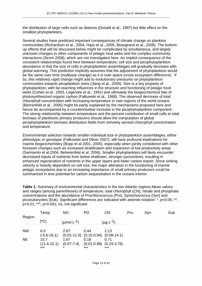
the distribution of large cells such as diatoms (Donald et al., 1997) but little effect on the smallest phytoplankters. Several studies have predicted important consequences of climate change on plankton communities (Richardson et al., 2004, Hays et al., 2005, Beaugrand et al., 2008). The bottom-up effects that will be discussed below might be complicated by simultaneous, and largely unknown changes to other components of pelagic food webs and the complex community interactions (Strom 2008), which are not investigated here. An implicit consequence of the consistent relationships found here between temperature, cell size and picophytoplankton abundance is that the size of cells in phytoplankton assemblages will gradually decrease with global warming. This prediction implicitly assumes that the adjustment of phytoplankton would be the same over time (multiyear change) as it is over space (cross ecosystem difference). If so, this relatively rapid change might add to evolutionary pressures on phytoplankton communities towards picoplankton sizes (Jiang et al., 2005). Size is a key property of phytoplankton, with far-reaching influences in the structure and functioning of pelagic food webs (Cohen et al., 2003, Legendre et al., 1991) and ultimately the biogeochemical fate of photosynthesized organic carbon (Falkowski et al., 1998). The observed decrease of total chlorophyll concentration with increasing temperature in vast regions of the world oceans (Behrenfeld et al., 2006) might be partly explained by the mechanisms proposed here and hence be accompanied by a counterintuitive increase in the picophytoplankton component. The strong relationship between temperature and the percent contribution of small cells to total biomass of planktonic primary producers should allow the computation of global picophytoplankton biomass distribution fields from remotely sensed chlorophyll concentration and temperature. Environmental selection towards smaller individual size in phytoplankton assemblages, either phenotypic or genotypic (Falkowski and Oliver 2007), will have profound implications for marine biogeochemistry (Bopp et al 2001, 2005), especially when jointly considered with other foreseen changes such as increased stratification and expansion of low productivity areas (Sarmiento et al.2004, Beherenfeld et al. 2006). Smaller phytoplankters will likely encounter decreased inputs of nutrients from below shallower, stronger pycnoclines, resulting in enhanced regeneration of nutrients in the upper layers and lower carbon export. Since sinking velocity is heavily dependent on cell size, the major alteration in the functioning of marine pelagic ecosystems due to an increasing importance of small primary producers could be summarized in less potential for carbon sequestration in the oceans interior. Table 1. Summary of environmental characteristics in the two Atlantic regions.Mean values and ranges (among parentheses) of temperature, total chlorophyll (Chl), nitrate and phosphate concentrations and the abundance of Prochlorococcus (Pro), Synechococcus (Syn) and picoeukaryotes (Euk). Significant differences are indicated with asterisk notation: *, p<0.05; **, p<0.01; ***, p<0.001; ns, not significant Region
Temp NO PO Chl Pro Syn Euk
(ºC) (µmol L-1) (µg L-1)
NW 6.0
(-0.6-16.1) 2.67 (0.01-11.0)
0.44 (0.15-0.94)
2.13 (0.08-14.1)
NE 15.7 (11.6-22.1)
1.67 (0.07-7.4)
0.18 (0.01-0.88)
0.71 (0.19-3.76)
*** * *** ***
EC FP7 MEECE | 212085 | D1.4 | New model parameterisations, Part B: Metabolic Theory
Page 14 of 42
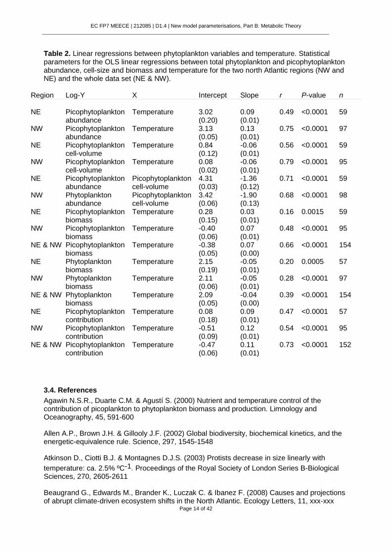
Table 2. Linear regressions between phytoplankton variables and temperature. Statistical parameters for the OLS linear regressions between total phytoplankton and picophytoplankton abundance, cell-size and biomass and temperature for the two north Atlantic regions (NW and NE) and the whole data set (NE & NW).
Region Log-Y X Intercept Slope r P-value n NE Picophytoplankton
abundance Temperature 3.02
(0.20) 0.09 (0.01)
0.49 <0.0001 59
NW Picophytoplankton abundance
Temperature 3.13 (0.05)
0.13 (0.01)
0.75 <0.0001 97
NE Picophytoplankton cell-volume
Temperature 0.84 (0.12)
-0.06 (0.01)
0.56 <0.0001 59
NW Picophytoplankton cell-volume
Temperature 0.08 (0.02)
-0.06 (0.01)
0.79 <0.0001 95
NE Picophytoplankton abundance
Picophytoplankton cell-volume
4.31 (0.03)
-1.36 (0.12)
0.71 <0.0001 59
NW Phytoplankton abundance
Picophytoplankton cell-volume
3.42 (0.06)
-1.90 (0.13)
0.68 <0.0001 98
NE Picophytoplankton biomass
Temperature 0.28 (0.15)
0.03 (0.01)
0.16 0.0015 59
NW Picophytoplankton biomass
Temperature -0.40 (0.06)
0.07 (0.01)
0.48 <0.0001 95
NE & NW Picophytoplankton biomass
Temperature -0.38 (0.05)
0.07 (0.00)
0.66 <0.0001 154
NE Phytoplankton biomass
Temperature 2.15 (0.19)
-0.05 (0.01)
0.20 0.0005 57
NW Phytoplankton biomass
Temperature 2.11 (0.06)
-0.05 (0.01)
0.28 <0.0001 97
NE & NW Phytoplankton biomass
Temperature 2.09 (0.05)
-0.04 (0.00)
0.39 <0.0001 154
NE Picophytoplankton contribution
Temperature 0.08 (0.18)
0.09 (0.01)
0.47 <0.0001 57
NW Picophytoplankton contribution
Temperature -0.51 (0.09)
0.12 (0.01)
0.54 <0.0001 95
NE & NW Picophytoplankton contribution
Temperature -0.47 (0.06)
0.11 (0.01)
0.73 <0.0001 152
3.4. References
Agawin N.S.R., Duarte C.M. & Agustí S. (2000) Nutrient and temperature control of the contribution of picoplankton to phytoplankton biomass and production. Limnology and Oceanography, 45, 591-600
Allen A.P., Brown J.H. & Gillooly J.F. (2002) Global biodiversity, biochemical kinetics, and the energetic-equivalence rule. Science, 297, 1545-1548
Atkinson D., Ciotti B.J. & Montagnes D.J.S. (2003) Protists decrease in size linearly with
temperature: ca. 2.5% ºC-1. Proceedings of the Royal Society of London Series B-Biological Sciences, 270, 2605-2611
Beaugrand G., Edwards M., Brander K., Luczak C. & Ibanez F. (2008) Causes and projections of abrupt climate-driven ecosystem shifts in the North Atlantic. Ecology Letters, 11, xxx-xxx
EC FP7 MEECE | 212085 | D1.4 | New model parameterisations, Part B: Metabolic Theory
Page 15 of 42
Behrenfeld M.J., O'Malley R.T., Siegel D.A., McClain C.R., Sarmiento J.L., Feldman G.C., Milligan A.J., Falkowski P.G., Letelier R.M. & Boss E.S. (2006) Climate-driven trends in contemporary ocean productivity. Nature, 444, 752-755
Bell T. & Kalff J. (2001) The contribution of picophytoplankton in marine and freshwater communities of different trophic status and depth. Limnol. Oceanogr., 46, 1243-1248
Bopp L., Monfray P., Aumont O., Dufresne J.L., Le Treut H., Madec G., Terray L. & Orr J.C. (2001) Potential impact of climate change on marine export production. Global Biogeochemical Cycles, 15, 81-99
Cohen J.E., Jonsson T. & Carpenter S.R. (2003) Ecological community description using the food web, species abundance, and body size. Proceedings of the National Academy of Sciences of the United States of America, 100, 1781-1786
Chisholm S.W. (1992) Phytoplankton size. In: Primary productivity and biogeochemical cycles in the sea (eds. Falkowski PG & Woodhead AD), pp. 213-237. Plenum Press, New York
Davey M., Tarran G.A., Mills M.M., Ridame C., Geider R.J. & LaRoche J. (2008) Nutrient limitation of picophytoplankton photosynthesis and growth in the tropical North Atlantic. Limnology and Oceanography, 53, 1722-1733
Donald K.M., Scanlan D.J., Carr N.G., Mann N.H. & Joint I. (1997) Comparative phosphorus nutrition of the marine cyanobacterium Synechococcus WH7803 and the marine diatom Thalassiosira weissflogii. Journal of Plankton Research, 19, 1793-1813
Doolittle D.F., Li W.K.W. & Wood M.W. (2008) Wintertime abundance of picoplankton in the Atlantic sector of the Southern Ocean. Nova Hedwigia, 133, 147-160
Falkowski P.G., Barber R.T. & Smetacek V. (1998) Biochemical controls and feedbacks on oceanic primary production. Science, 281, 200-206
Finkel Z.V., Irwin A.J. & Schofield O. (2004) Resource limitation alters the 3/4 size scaling of metabolic rates in phytoplankton. Marine Ecology-Progress Series, 273, 269-279
Gillooly J.F., Brown J.H., West G.B., Savage V.M. & Charnov E.L. (2001) Effects of size and temperature on metabolic rate. Science, 293, 2248-2251
Harris G.P. (1986) Phytoplankton ecology. Structure, function and fluctuations. Chapman and Hall.
Hays G.C., Richardson A.J. & Robinson C. (2005) Climate change and marine plankton. Trends in Ecology & Evolution, 20, 337-344
Jiang L., Schofield O.M.E. & Falkowski P.G. (2005) Adaptive evolution of phytoplankton cell size. American Naturalist, 166, 496-505
Kamykowski D., Zentara S.J., Morrison J.M. & Switzer A.C. (2002) Dynamic global patterns of nitrate, phosphate, silicate, and iron availability and phytoplankton community composition from remote sensing data. Global Biogeochemical Cycles, 16, -
Legendre L. & Le Fèvre J. (1991) From individual plankton cells to pelagic marine ecosystems and to global biogeochemical cycles. In: Particle analysis in oceanography (ed. Demers S), pp. 261-300

EC FP7 MEECE | 212085 | D1.4 | New model parameterisations, Part B: Metabolic Theory
Page 16 of 42
Li W.K.W. (1998) Annual average abundance of heterotrophic bacteria and Synechococcus in surface ocean waters. Limnology and Oceanography, 43, 1746-1753
Li W.K.W. (2002) Macroecological patterns of phytoplankton growth in the northwestern North Atlantic Ocean. Nature, 419, 154-157
Li W.K.W. & Harrison W.G. (2008) Propagation of an atmospheric climate signal to phytoplankton in a small marine basin. Limnology and Oceanography, 53, 1734-1745
Li W.K.W., Harrison W.G. & Head E.J.H. (2006) Coherent assembly of phytoplankton communities in diverse temperate ocean ecosystems. Proceedings of the Royal Society B-Biological Sciences, 273, 1953-1960
Moon-van der Staay S.Y., De Wachter R. & Vaulot D. (2001) Oceanic 18S rDNA sequences from picoplankton reveal unsuspected eukaryotic diversity. Nature, 409, 607-610
Morán X.A.G. (2007) Annual cycle of picophytoplankton photosynthesis and growth rates in a temperate coastal ecosystem: a major contribution to carbon fluxes. Aquatic Microbial Ecology, 49, 267-279
Not F., Valentin K., Romari K., Lovejoy C., Massana R., Töbe K., Vaulot D. & Medlin L.K. (2007) Picobiliphytes: A marine picoplanktonic algal group with unknown affinities to other eukaryotes. Science, 315, 253-255
Partensky F., Blanchot J. & Vaulot D. (1999) Differential distribution and ecology of Prochlorococcus and Synechococcus in oceanic waters: a review. Bull. Inst. Océanogr. Monaco, 19, 457-475
Raven J.A. (1998) The twelfth Tansley Lecture. Small is beautiful: the picophytoplankton. Functional Ecology, 12, 503-513
Richardson A.J. & Schoeman D.S. (2004) Climate impact on plankton ecosystems in the Northeast Atlantic. Science, 305, 1609-1612
Richardson T.L. & Jackson G.A. (2007) Small phytoplankton and carbon export from the surface ocean. Science, 315, 838-840
Sieburth J.M., Smetacek V. & Lenz J. (1978) Pelagic Ecosystem Structure - Heterotrophic Compartments of Plankton and Their Relationship to Plankton Size Fractions - Comment. Limnology and Oceanography, 23, 1256-1263
White E.P., Ernest S.K.M., Kerkhoff A.J. & Enquist B.J. (2007) Relationships between body size and abundance in ecology. Trends in Ecology & Evolution, 22, 323-330
Worden A.Z., Nolan J.K. & Palenik B. (2004) Assessing the dynamics and ecology of marine picophytoplankton: The importance of the eukaryotic component. Limnol. Oceanogr., 49, 168-179
4. Temperature, nutrients and the size-scaling of phytoplankton growth in the

EC FP7 MEECE | 212085 | D1.4 | New model parameterisations, Part B: Metabolic Theory
Page 17 of 42
sea
4.1. Summary
The effects of cell size on phytoplankton mass-specific growth rate were re-analysed using a compilation of field measurements from surface waters around the world published by Chen and Liu (2010). After correcting for the effects of temperature, Chen and Liu (2010) analysis indicates that there is a modal size around 2.8-5.8 μm where mass-specific growth is maximal. As Chen and Liu (2010) acknowledge, their analysis contrasts with allometric scaling theories that predict a continuous decrease of mass-specific growth rate with increasing size (Brown et al. 2004; Lopez-Urrutia et al. 2006). In contrast, Chen and Liu’s (2010) analysis shows that bellow the modal size, that is in the pico- to nano-phytoplankton size range, growth rate increases with cell size. They argue that the unimodal pattern stems from picoplankton having evolved to have inherently low growth rates, independently of nutrient availability. Here we argue that the unimodal pattern they obtain might be due to an incorrect temperature correction and to an internal inconsistency in their database because a large portion of their picoplankton data contains a correction for photoacclimation effects, while the rest of their data do not.
4.2. Methods
To carry out their study, Chen and Liu (2010) used two data sets, one from C incorporation and a second from dilution experiments. In both data sets, a unimodal pattern between mass-specific growth rate and cell size emerges. In these two data sets, however, cell size is correlated with nutrient availability, so it could be argued that, rather than a direct effect of cell size, the lower growth rates of smaller phytoplankton could be due to these organisms living under resource limitation (Raven 1998), (fig.1C in Chen and Liu 2010). Chen and Liu (2010) tried to resolve these confounding effects due to correlation between nutrient availability and cell size by using a data set of phytoplankton growth rates measured under nutrient enrichment. The unimodal pattern still apparent in this nutrient-saturated dilution data set is probably the most striking result in their analysis. Chen and Liu (2010) concluded that the lower growth rates in the picoplankton size range are an adaptive feature rather than a direct consequence of nutrient limitation.
4.3. Results
We consider whether this pattern is due to a bias in the data compilation. In an effort to get the best data available, Chen and Liu (2010) used phytoplankton growth rates with a correction for photoacclimation for the two data sources that had this information available, while the rest of their nutrient-enriched dilution data are uncorrected. These corrected data happen to correspond to most of the low values in the picoplankton size range (Fig. 6A). If we take this nutrient-enriched dilution data set and replace these photoacclimation-corrected data by the uncorrected values comparable to the rest of the data set, the unimodal pattern is no longer evident (Fig. 6B). The quadratic term in the unimodal fit is no longer significant ( -test, = -
1.255, df = 255, = 0.211). Although now a linear fit is more appropriate, the linear relationship obtained is not what the metabolic theory of ecology (MTE) predicts. MTE predicts
that metabolic rates and organism biovolume (BV) should scale as (West et al.
1999; Lopez-Urrutia et al., 2006). Hence, size-specific metabolic rates ( ), such
as individual growth rate, should scale as . Chen and Liu (2010) defines cell size as the carbon content. Lopez-Urrutia et al. (2006) have shown that, when phytoplankton cell size is expressed in units of carbon instead of biovolume, phytoplankton
growth rate scales isometrically with cell size ( ), so carbon-specific growth
rate ( ) should be independent of cell carbon. This is due to phytoplankton
carbon content and biovolume scaling as (Strathmann 1967), so
.
EC FP7 MEECE | 212085 | D1.4 | New model parameterisations, Part B: Metabolic Theory
Page 18 of 42
Hence, following MTE, a plot of carbon-specific growth rate should yield no significant relationship with cell-carbon, whereas Fig. 6B shows a positive relationship. We think that this
trend could be due to the temperature correction used. Chen and Liu (2010) used a of 1.88 (Eppley 1972; Bissinger et al. 2008) so that -0.0275 T is the temperature-corrected phytoplankton specific growth rate, where T is the temperature in Celsius. On the other hand, MTE uses the Van’t Hoff - Arrhenius equation (Arrhenius 1915) to describe the effects of temperature on metabolic rates:
(1)
where k is Boltzmann’s constant ( ), is the absolute temperature (in Kelvin) and E is the average activation energy for the metabolic process under study. For autotrophs the effective activation energy for photosynthetic reactions should be close to 0.32 eV Allen et al. (2005). In the case of photosynthesis, the Van’t Hoff-Arrhenius equation is just an approximation to a more complex process (Farquhar et al. 1980). The activation energy of 0.32 predicted by MTE is based on data from the effects of temperature on several photosynthetic processes ( appendix in Allen et al. 2005). Lopez-Urrutia et al. (2006) obtained effective activation energies for phytoplankton growth rates of 0.29 eV, not significantly different from the predicted value of 0.32 eV.
The in turn is an approximation to Van’t Hoff - Arrehnius equation, so both temperature
coefficients, E and , are interrelated by equation = where is
273.15 K ( box 1 in Gillooly et al. 2002). Hence, the of 1.88 from Eppley (1972) is equivalent to an activation energy of approximately 0.405 eV, which is slightly higher than the activation energy predicted for autotrophs and the empirical value obtained by Lopez-Urrutia et al. (2006). If growth rates from the nutrient-enriched dilution data set are plotted against temperature, the resultant activation energy is 0.36 eV (Fig. 2), which is not significantly
different from the value predicted by MTE ( -test, = 2.08, df = 256, = 0.15) but significantly
lower than the value used by Chen and Liu (2010) ( -test, = 12.522, df = 256, 0.001). This subtle difference between the two temperature corrections might be responsible for the pattern obtained in Fig. 1B. If instead of the temperature correction used by Chen and Liu
(2010) based on Eppley’s (1972) , we use the temperature correction based on MTE and
the theoretical activation energy of 0.32 eV (equivalent to a of 1.64), we obtain no significant relationship between carbon-specific growth rate and average cell carbon (Fig. 6C),
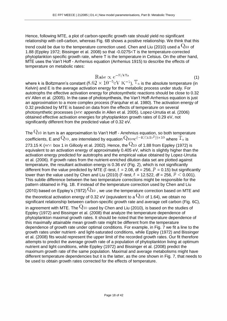
in agreement with MTE. The used by Chen and Liu (2010), is based on the studies of Eppley (1972) and Bissinger et al. (2008) that analyze the temperature dependence of phytoplankton maximal growth rates. It should be noted that the temperature dependence of this maximally attainable mean growth rate might be different from the temperature dependence of growth rate under optimal conditions. For example, in Fig. 7 we fit a line to the growth rates under nutrient- and light-saturated conditions, while Eppley (1972) and Bissinger et al. (2008) fits would represent the upper limit of the recorded growth rates. Our fit therefore attempts to predict the average growth rate of a population of phytoplankton living at optimum nutrient and light conditions, while Eppley (1972) and Bissinger et al. (2008) predict the maximum growth rate of the same population. Maximal and average metabolisms might have different temperature dependencies but it is the latter, as the one shown in Fig. 7, that needs to be used to obtain growth rates corrected for the effects of temperature.

EC FP7 MEECE | 212085 | D1.4 | New model parameterisations, Part B: Metabolic Theory
Page 19 of 42
Figure 6. Relationship between temperature-corrected growth rate and average cell size(M) for the nutrient-enriched dilution data set. (A) Chen and Liu (2010) data. Grey filled symbols correspond to photoacclimation-corrected data. The solid line correspond to a linear fit ( ; ANOVA: = 0.14, = 261, -value 0.001). The dashed line correspond to a quadratic fit ( ; ANO-VA: = 0.17, = 261, -value 0.001). (B) Same as (A) but with all data uncorrected for photoacclimation. The solid line correspond to a linear fit ( ; ANOVA: = 0.09, = 258, -value 0.001). The dashed line correspond to a quadratic fit ( ; ANOVA: = 0.10, = 258, -value 0.001). (C) Same as (B) but using the temperature correction based on MTE. In this panel, just a linear fit is shown ( ; ANOVA: = 0.01, = 258, -value = 0.203).
When inferring the effect on metabolic processes of variables that might be correlated with temperature, like body size or nutrients, it should be borne in mind that the value used for the temperature correction might introduce some bias. We believe that the value used for the temperature correction should be derived theoretically, as the one used in Fig. 6C, and not empirically, because solely based on a field data set like the one under analysis, it is impossible to discern the magnitude of the effects of temperature and of variables correlated with it. For example, it could be argued that the temperature coefficient we obtain in Fig. 7 is dependent on the assumption that weight-specific growth rate is independent of cell size, and that if we had corrected growth rate by the cell-size effects obtained in Fig. 6B, we would have obtained a temperature coefficient closer to Eppley’s (1972). To avoid this caveat, the temperature coefficient used should be based on some theory, like the one we used based on MTE, or corroborated by experimental work where the effect of the other variables can be controlled. Such a criticism can be applied also, for example, to the activation energy of 0.29 eV for cell-size corrected phytoplankton growth rate obtained by Lopez-Urrutia et al. (2006). This value is to some extent dependent on the assumption that growth rate scales with cell size to the 3/4 power. As cell size and temperature are correlated, taking a theoretical value for the effects of cell size to evaluate the effects of temperature, conditions in some way the activation energy obtained. A similar criticism can be made of field studies of the effects of cell size that do not take into account the effects of temperature or nutrient availability. For example, the results of Maranon (2008), who obtains an almost isometric scaling between phytoplankton production rates and cell volume, are dependent on the unlikely assumption that rates measured for the smallest cells do not coincide with the lowest nutrient levels.
EC FP7 MEECE | 212085 | D1.4 | New model parameterisations, Part B: Metabolic Theory
Page 20 of 42
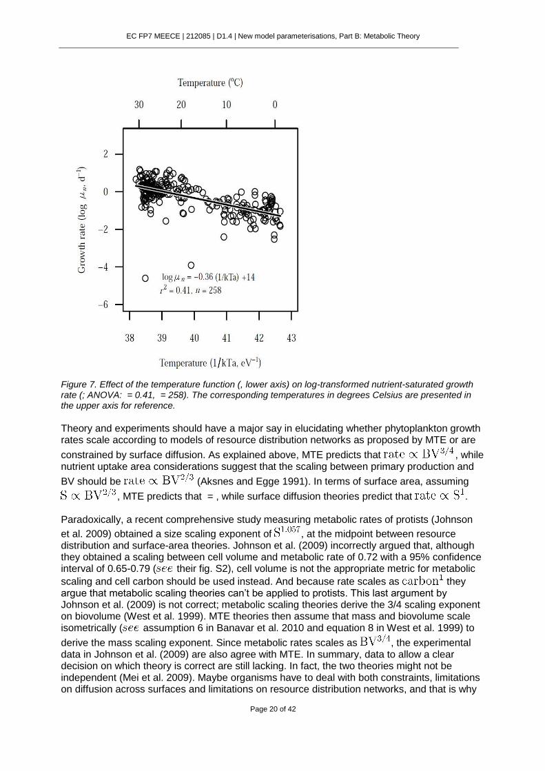
Figure 7. Effect of the temperature function (, lower axis) on log-transformed nutrient-saturated growth rate (; ANOVA: = 0.41, = 258). The corresponding temperatures in degrees Celsius are presented in the upper axis for reference.
Theory and experiments should have a major say in elucidating whether phytoplankton growth rates scale according to models of resource distribution networks as proposed by MTE or are
constrained by surface diffusion. As explained above, MTE predicts that , while nutrient uptake area considerations suggest that the scaling between primary production and
BV should be (Aksnes and Egge 1991). In terms of surface area, assuming
, MTE predicts that = , while surface diffusion theories predict that . Paradoxically, a recent comprehensive study measuring metabolic rates of protists (Johnson
et al. 2009) obtained a size scaling exponent of , at the midpoint between resource distribution and surface-area theories. Johnson et al. (2009) incorrectly argued that, although they obtained a scaling between cell volume and metabolic rate of 0.72 with a 95% confidence interval of 0.65-0.79 ( their fig. S2), cell volume is not the appropriate metric for metabolic
scaling and cell carbon should be used instead. And because rate scales as they argue that metabolic scaling theories can’t be applied to protists. This last argument by Johnson et al. (2009) is not correct; metabolic scaling theories derive the 3/4 scaling exponent on biovolume (West et al. 1999). MTE theories then assume that mass and biovolume scale isometrically ( assumption 6 in Banavar et al. 2010 and equation 8 in West et al. 1999) to
derive the mass scaling exponent. Since metabolic rates scales as , the experimental data in Johnson et al. (2009) are also agree with MTE. In summary, data to allow a clear decision on which theory is correct are still lacking. In fact, the two theories might not be independent (Mei et al. 2009). Maybe organisms have to deal with both constraints, limitations on diffusion across surfaces and limitations on resource distribution networks, and that is why
EC FP7 MEECE | 212085 | D1.4 | New model parameterisations, Part B: Metabolic Theory
Page 21 of 42
the measured scaling exponent is at the midpoint (Banavar et al. 2010).
4.4. References
Aksnes, D. L., and J. K. Egge. 1991. A theoretical-model for nutrient-uptake In phytoplankton. Marine Ecology-progress Series : 65–72.
Allen, A. P., J. F. Gillooly, and J. H. Brown. 2005. Linking the global carbon cycle to individual metabolism. Functional Ecology : 202–213.
Arrhenius, S. 1915. Quantitative laws in biological chemistry. London.
Banavar, J. R., M. E. Moses, J. H. Brown, J. Damuth, A. Rinaldo, R. M. Sibly, and A. Maritan. 2010. A general basis for quarter-power scaling in animals. Proceedings of the National Academy of Sciences of the United States of America : 15816–15820.
Bissinger, J. E., D. J. S. Montagnes, J. Sharples, and D. Atkinson. 2008. Predicting marine phytoplankton maximum growth rates from temperature: Improving on the Eppley curve using quantile regression. Limnology and Oceanography : 487–493.
Brown, J. H., J. F. Gillooly, A. P. Allen, V. M. Savage, and G. B. West. 2004. Toward a metabolic theory of ecology. Ecology : 1771–1789.
Chen, B. Z., and H. B. Liu. 2010. Relationships between phytoplankton growth and cell size in surface oceans: Interactive effects of temperature, nutrients, and grazing. Limnology and Oceanography : 965–972.
Eppley, R. W. 1972. Temperature and phytoplankton growth in sea. Fishery Bulletin : 1063–1085.
Farquhar, G. D., S. V. Caemmerer, and J. A. Berry. 1980. A biochemical-model of photosynthetic CO2 assimilation in eaves of C-3 species. Planta : 78–90.
Gillooly, J. F., E. L. Charnov, G. B. West, V. M. Savage, and J. H. Brown. 2002. Effects of size and temperature on developmental time. Nature : 70–73.
Johnson, M. D., J. Volker, H. V. Moeller, E. Laws, K. J. Breslauer, and P. G. Falkowski. 2009. Universal constant for heat production in protists. Proceedings of the National Academy of Sciences of the United States of America : 6696–6699.
Lopez-Urrutia, A., E. San Martin, R. P. Harris, and X. Irigoien. 2006. Scaling the metabolic balance of the oceans. Proceedings Of The National Academy Of Sciences Of The United States Of America : 8739–8744.
Maranon, E. 2008. Inter-specific scaling of phytoplankton production and cell size in the field. Journal Of Plankton Research : 157–163.
Mei, Z. P., Z. V. Finkel, and A. J. Irwin. 2009. Light and nutrient availability affect the size-scaling of growth in phytoplankton. Journal of Theoretical Biology : 582–588.
Raven, J. A. 1998. The twelfth Tansley Lecture. Small is beautiful: the picophytoplankton. Functional Ecology : 503–513.
Strathmann, R. 1967. Estimating the organic carbon content of phytoplankton from cell volume or plasma volume. Limnology : 411–418.
EC FP7 MEECE | 212085 | D1.4 | New model parameterisations, Part B: Metabolic Theory
Page 22 of 42
West, G. B., J. H. Brown, and B. J. Enquist. 1999. The fourth dimension of life: Fractal geometry and allometric scaling of organisms. Science : 1677–1679.
5. The evolution of high prey capture rates in planktivorous fish and jellyfish
5.1. Summary
Fish have compact, slender bodies, and use their eyes to detect prey. In contrast, cruising medusae pulse their watery, bell-shaped bodies, to vortex rings which generates a feeding current and transports water and prey through their tentacles and oral arms. Likewise, lobate ctenophores beat their auricular cilia to generate a feeding current by drawing water between their feeding lobes and past capture surfaces. Compared with visual predation, tactile feeding current predation is a primitive system dating back to the Ediacaran some 500 MYA ago. We may expect lower clearance rates of jellyfish when compared with visually predating fish, what would in turn explain the competitive prevalence of fish when they are not overfished. To test these predictions we have analyzed the data compiled in Task 1.1.
5.2 Methods
We have assumed that both respiration and clearance rates vary with body size and temperature according to the following model:
, where M stands for either clearance or respiration rate, B0 is a scaling constant, Ea is the
activation energy, k is Boltzmann's constant (0,0000862 eV/ºK), T is the absolute temperature (in ºK), B is body size in either carbon or wet weight units and b is a scaling exponent (as in ref. (Gillooly et al. 2001)). For the clearance rates, we have assumed that Ea=0.6 as for the
respiration rates (based on Gillooly et al. 2001). Allometric regressions were done with
temperature-corrected rates, which were obtained by dividing the measured rates by . Comparisons of log(respiration rates) and log(clearance rates) among groups of organisms were done by means of the general linear model, with either log (body carbon) or log(wet weight) as covariate, taxonomic or functional group as factor and using the R software (http://www.r-project.org/). Heterogeneity of slopes was tested through the interaction between covariate and factor. If not significant, we proceeded to a test of significance of the factor, or ANCOVA, this time without interaction term.
5.3 Results
Clearance rates of jellyfish were not significantly different from those of visually predating fish with the same carbon content (ANCOVA, P=0.52; See Methods for tests; Fig. 8a). Both jellyfish and raptorial fish scan the water at least 10 times faster than filter feeding fish and crustaceans with feeding modes ranging from filter feeding to raptorial feeding by mechano or chemo detection (slopes were heterogeneous, P<0.001, Fig. 8A). However, jellyfish respire just as much as any animal with similar body carbon (ANCOVA, P=0.072; Fig. 8c). These rates can be used to calculate the energy available for growth and reproduction, or scope for growth.

EC FP7 MEECE | 212085 | D1.4 | New model parameterisations, Part B: Metabolic Theory
Page 23 of 42
Figure 8. Allometry of prey capture and metabolism in jellyfish. Temperature-corrected clearance (a-b) and respiration rates (c-d) of jellyfish, fish and their crustacean prey vs. body carbon (a-c) or body wet weight (b-d, see Methods for temperature correction). Thick lines indicate Ordinary Least Squares log-log fits, and yellow squares with grey arrows indicate which data were pooled to construct each regression line. Pooling was done following statistical tests for homogeneity of slopes and intercepts
EC FP7 MEECE | 212085 | D1.4 | New model parameterisations, Part B: Metabolic Theory
Page 24 of 42
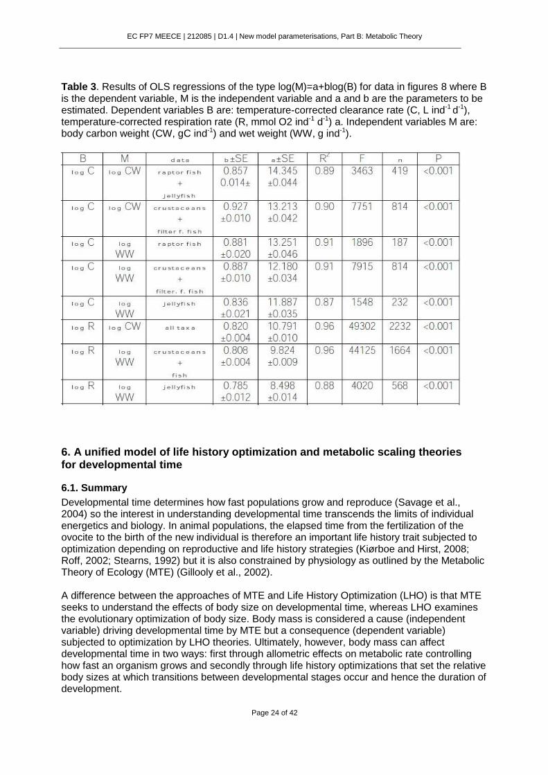
Table 3. Results of OLS regressions of the type log(M)=a+blog(B) for data in figures 8 where B is the dependent variable, M is the independent variable and a and b are the parameters to be estimated. Dependent variables B are: temperature-corrected clearance rate (C, L ind-1 d-1), temperature-corrected respiration rate (R, mmol O2 ind-1 d-1) a. Independent variables M are: body carbon weight (CW, gC ind-1) and wet weight (WW, g ind-1).
6. A unified model of life history optimization and metabolic scaling theories for developmental time
6.1. Summary
Developmental time determines how fast populations grow and reproduce (Savage et al., 2004) so the interest in understanding developmental time transcends the limits of individual energetics and biology. In animal populations, the elapsed time from the fertilization of the ovocite to the birth of the new individual is therefore an important life history trait subjected to optimization depending on reproductive and life history strategies (Kiørboe and Hirst, 2008; Roff, 2002; Stearns, 1992) but it is also constrained by physiology as outlined by the Metabolic Theory of Ecology (MTE) (Gillooly et al., 2002). A difference between the approaches of MTE and Life History Optimization (LHO) is that MTE seeks to understand the effects of body size on developmental time, whereas LHO examines the evolutionary optimization of body size. Body mass is considered a cause (independent variable) driving developmental time by MTE but a consequence (dependent variable) subjected to optimization by LHO theories. Ultimately, however, body mass can affect developmental time in two ways: first through allometric effects on metabolic rate controlling how fast an organism grows and secondly through life history optimizations that set the relative body sizes at which transitions between developmental stages occur and hence the duration of development.
EC FP7 MEECE | 212085 | D1.4 | New model parameterisations, Part B: Metabolic Theory
Page 25 of 42
Reconciling MTE and LHO approaches has remained an elusive problem in ecology. Despite the copious empirical support given to both MTE and LHO perspectives, we still lack a general model for embryo development time (EDT) considering them simultaneously. The aim of the present work is to establish a link between MTE and LHO using the ontogenetic growth model of West et al. (2001) and Smith and Fretwell (1974) model for optimal offspring size. We will show that it is possible to unify in a single model the effects of allometric constraints and reproductive trade-offs on developmental time.
6.2 The model
We will first introduce the OGM as developed by West et al. (2001) and the trade-off between size and number of offspring as formulated by Charnov and Ernest (2006). Finally we will show that it is possible to combine both theories in a merged model.
6.2.1 The MTE approach
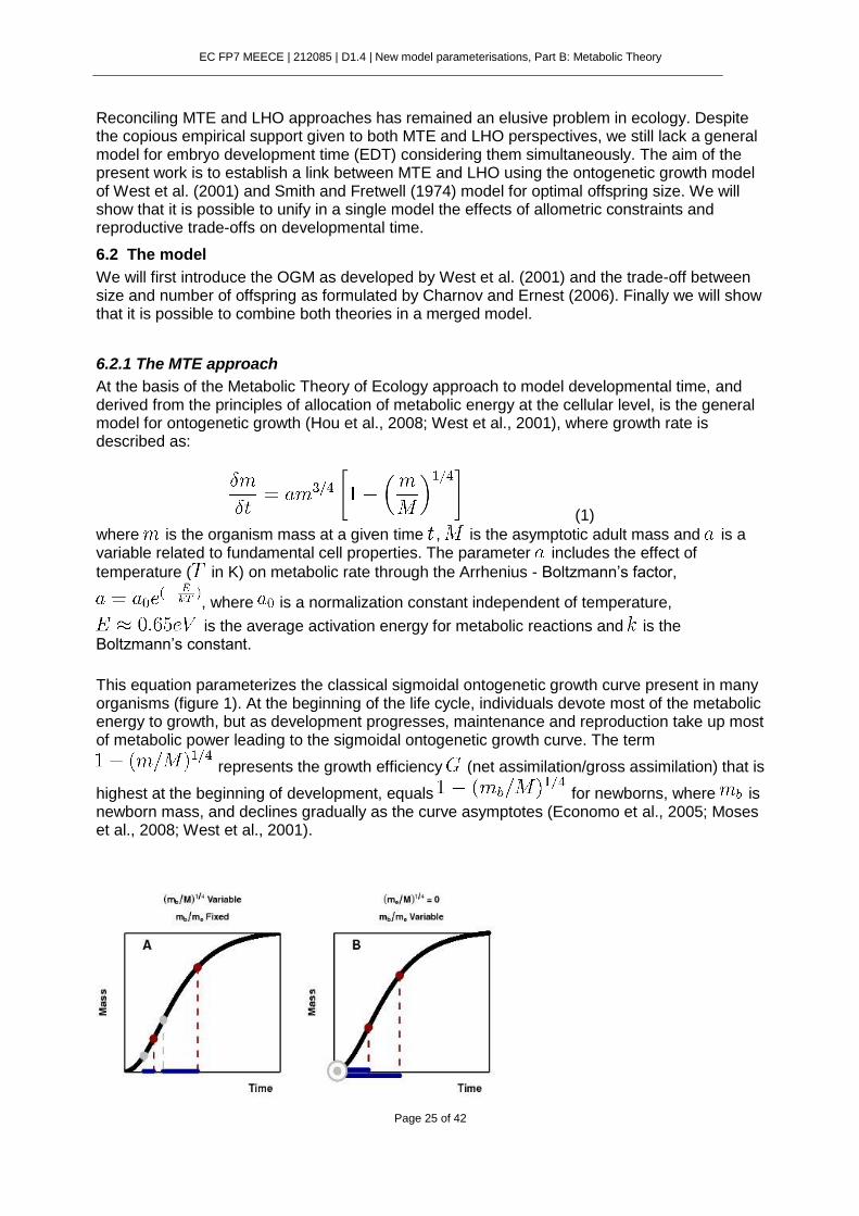
At the basis of the Metabolic Theory of Ecology approach to model developmental time, and derived from the principles of allocation of metabolic energy at the cellular level, is the general model for ontogenetic growth (Hou et al., 2008; West et al., 2001), where growth rate is described as:
(1)
where is the organism mass at a given time , is the asymptotic adult mass and is a variable related to fundamental cell properties. The parameter includes the effect of
temperature ( in K) on metabolic rate through the Arrhenius - Boltzmann’s factor,
, where is a normalization constant independent of temperature,
is the average activation energy for metabolic reactions and is the Boltzmann’s constant.
This equation parameterizes the classical sigmoidal ontogenetic growth curve present in many organisms (figure 1). At the beginning of the life cycle, individuals devote most of the metabolic energy to growth, but as development progresses, maintenance and reproduction take up most of metabolic power leading to the sigmoidal ontogenetic growth curve. The term
represents the growth efficiency (net assimilation/gross assimilation) that is
highest at the beginning of development, equals for newborns, where is newborn mass, and declines gradually as the curve asymptotes (Economo et al., 2005; Moses et al., 2008; West et al., 2001).
EC FP7 MEECE | 212085 | D1.4 | New model parameterisations, Part B: Metabolic Theory
Page 26 of 42
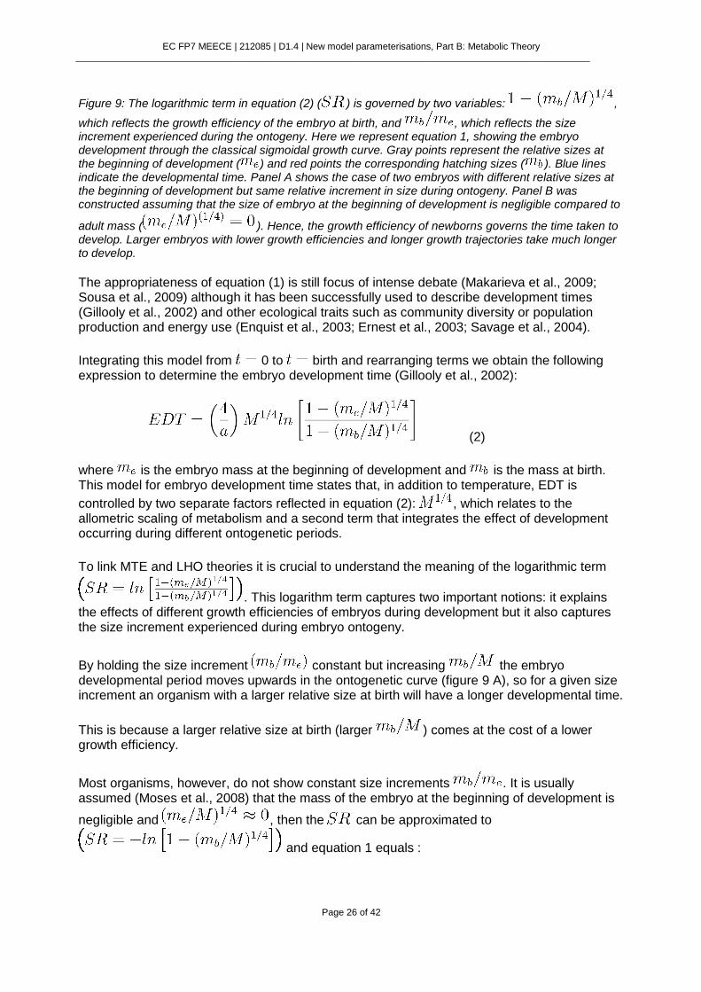
Figure 9: The logarithmic term in equation (2) ( ) is governed by two variables: ,
which reflects the growth efficiency of the embryo at birth, and , which reflects the size increment experienced during the ontogeny. Here we represent equation 1, showing the embryo development through the classical sigmoidal growth curve. Gray points represent the relative sizes at the beginning of development ( ) and red points the corresponding hatching sizes ( ). Blue lines indicate the developmental time. Panel A shows the case of two embryos with different relative sizes at the beginning of development but same relative increment in size during ontogeny. Panel B was constructed assuming that the size of embryo at the beginning of development is negligible compared to
adult mass ( ). Hence, the growth efficiency of newborns governs the time taken to develop. Larger embryos with lower growth efficiencies and longer growth trajectories take much longer to develop.
The appropriateness of equation (1) is still focus of intense debate (Makarieva et al., 2009; Sousa et al., 2009) although it has been successfully used to describe development times (Gillooly et al., 2002) and other ecological traits such as community diversity or population production and energy use (Enquist et al., 2003; Ernest et al., 2003; Savage et al., 2004).
Integrating this model from 0 to birth and rearranging terms we obtain the following expression to determine the embryo development time (Gillooly et al., 2002):
(2)
where is the embryo mass at the beginning of development and is the mass at birth. This model for embryo development time states that, in addition to temperature, EDT is
controlled by two separate factors reflected in equation (2): , which relates to the allometric scaling of metabolism and a second term that integrates the effect of development occurring during different ontogenetic periods.
To link MTE and LHO theories it is crucial to understand the meaning of the logarithmic term
. This logarithm term captures two important notions: it explains the effects of different growth efficiencies of embryos during development but it also captures the size increment experienced during embryo ontogeny.
By holding the size increment constant but increasing the embryo developmental period moves upwards in the ontogenetic curve (figure 9 A), so for a given size increment an organism with a larger relative size at birth will have a longer developmental time.
This is because a larger relative size at birth (larger ) comes at the cost of a lower growth efficiency.
Most organisms, however, do not show constant size increments . It is usually assumed (Moses et al., 2008) that the mass of the embryo at the beginning of development is
negligible and , then the can be approximated to
and equation 1 equals :

EC FP7 MEECE | 212085 | D1.4 | New model parameterisations, Part B: Metabolic Theory
Page 27 of 42
(3)
An increase in will result in an increase in the size increment experienced during development, resulting in longer developmental time (figure 9B).
6.2.2 LHO trade-offs
Life History Optimization (LHO) theories view body mass as a trait that can be optimized and try to understand the trade-offs that lead to different relative body sizes at the transitions between ontogenetic periods. For example, there is a trade-off between reaching maturity early or maturing later but being able to invest many resources in reproduction (Roff, 2002; Stearns, 1992). There is also a trade-off where reproductive resources are balanced between the size and the number of offspring (Smith and Fretwell, 1974). Hence, LHO theories make predictions on developmental time as a result of an optimizing evolutionary process (Hirst and Lopez-Urrutia, 2006; Kiørboe and Hirst 2008; Sibly and Brown, 2007, 2009).
The classic life history optimization model of Smith and Fretwell (1974) describes how the daily
offspring production rate, , is directly related to the amount of resources allocated to
reproduction in a reproductive event, , and inversely related to the allocation per offspring, ,
( ). Charnov and Ernest (2006) suggested that, in mammals, the investment per offspring is well approximated by the offspring mass at birth while the resources diverted to
reproduction scale with adult mass raised to . They showed that the relationship
was supported with data for mammals.
Hence, Smith and Fretwell model for optimal offspring size can be summarized by the equation
, where is a scaling constant, which leads to .
6.2.3 An ensembled model of MTE and LHO
The similarity between the mass ratios in the logarithmic term
of the ontogenetic growth model (where is adult mass and is the newborn mass) and Charnov and Ernest (2006) relationship,
(where is the daily offspring production rate and is a constant) allows to combine both theories.
Solving Charnov-Ernest relationship for yields
and substituting this expression in the term we arrive at:
(4)
In this new form of the ontogenetic growth model, the value of the term depends on the
daily offspring production rate raised to the power and on the mass of the newborn with
an exponent of as well as on a scaling constant . This combined model predicts that for a given body mass and temperature, the trade off between number and offspring size leads

EC FP7 MEECE | 212085 | D1.4 | New model parameterisations, Part B: Metabolic Theory
Page 28 of 42
to the prediction of an inverse relationship between developmental time and offspring number.
6.3 Materials and methods
To test these models, we compiled data on embryo development time, rearing temperature, and newborn mass of aquatic ectotherms, birds and mammals from the works of Gillooly et al. (2002), Visser and Beintema (1991) and Ernest (2003) respectively. To test the assumption in
equation 3 that is close to zero, we also tried to compile data on embryo weight at the beginning of development. These data are rarely available in the literature due to the methodological difficulties in its measurement. Nevertheless, we attempted to obtain rough estimates for the different groups considered.
Newborn weights of both birds and mammals were obtained from Visser and Beintema (1991) and Ernest (2003) respectively. For oviparous animals, when newborn weight was not available, it was assumed to equal the total egg weight (calculated from egg diameters
assuming a density of 1 g ml ). When egg development ends in fish and amphibians most organisms hold prominent yolk sacs that do not properly constitute newborn mass, as they represent energy reserves for future growth. We calculated an average percent yolk mass at birth for each group from the literature. It is important to note that these yolk sacs should not be considered in the mass at birth ( ) in the MTE equations, because they represent energy reserves that will be used for biomass synthesis during post-embryonic development. For Charnov and Ernest (2006) relationship, however, these yolk sacs should be considered as investment per offspring. This differentiation between two masses at birth is equivalent to the choice in using newborn or weaning mass in mammals (Charnov and Ernest, 2006). We
followed Charnov and Ernest (2006) in testing the relationship both with
equal to newborn mass and larvae mass not including yolk sac and with equal to weaning
mass and larvae mass with the yolk sac. For zooplankton and insects and were considered equal. Bird species considered here are nidifugous shorebirds for which parental investment per offspring is difficult to quantify after hatching. For this reason we assumed that
and were similar for birds.
To calculate the daily offspring production rate ( ) we compiled data on clutch/litter size and number of reproductive events in a year. For comparison, all rates were rescaled to the same time period resulting in a source of uncertainty as we could not account for time spent in torpor or hibernation in mammals. Hence, the rates for mammals, birds, iteroparous fish and amphibians were divided by 365 to obtain a offspring production rate per day. In the case of semelparous fish we divided the mean egg production by their total life span. For insects and zooplankters which usually have a life span shorter than 1 year we divided the total life-time egg production by the length of the adult life. In the case of univoltine insects, where adult life spans just for a few days but egg synthesis starts during the larval stage, we considered a reproductive cycle of one year. In some cases, the daily egg production rate of zooplankters was directly obtained from the literature. Another source of uncertainty in our compilation is that, for ectotherms, offspring production was available at the same temperature as developmental time only for a reduced portion of the data, for most species we used mean values of brood sizes under optimal conditions.
6.4 Results
6.4.1 MTE model: allometric, growth efficiency and size increment effects
Following equation 2 once EDT is corrected for the effects of temperature and the size
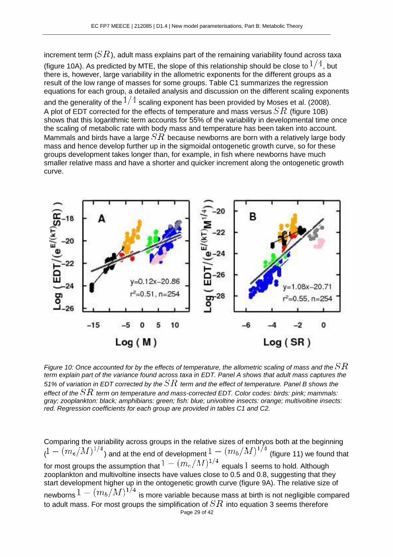
EC FP7 MEECE | 212085 | D1.4 | New model parameterisations, Part B: Metabolic Theory
Page 29 of 42
increment term ( ), adult mass explains part of the remaining variability found across taxa
(figure 10A). As predicted by MTE, the slope of this relationship should be close to , but there is, however, large variability in the allometric exponents for the different groups as a result of the low range of masses for some groups. Table C1 summarizes the regression equations for each group, a detailed analysis and discussion on the different scaling exponents
and the generality of the scaling exponent has been provided by Moses et al. (2008).
A plot of EDT corrected for the effects of temperature and mass versus (figure 10B) shows that this logarithmic term accounts for 55% of the variability in developmental time once the scaling of metabolic rate with body mass and temperature has been taken into account.
Mammals and birds have a large because newborns are born with a relatively large body mass and hence develop further up in the sigmoidal ontogenetic growth curve, so for these groups development takes longer than, for example, in fish where newborns have much smaller relative mass and have a shorter and quicker increment along the ontogenetic growth curve.
Figure 10: Once accounted for by the effects of temperature, the allometric scaling of mass and the term explain part of the variance found across taxa in EDT. Panel A shows that adult mass captures the
51% of variation in EDT corrected by the term and the effect of temperature. Panel B shows the
effect of the term on temperature and mass-corrected EDT. Color codes: birds: pink; mammals: gray; zooplankton: black; amphibians: green; fish: blue; univoltine insects: orange; multivoltine insects: red. Regression coefficients for each group are provided in tables C1 and C2.
Comparing the variability across groups in the relative sizes of embryos both at the beginning
( ) and at the end of development (figure 11) we found that
for most groups the assumption that equals seems to hold. Although zooplankton and multivoltine insects have values close to 0.5 and 0.8, suggesting that they start development higher up in the ontogenetic growth curve (figure 9A). The relative size of
newborns is more variable because mass at birth is not negligible compared
to adult mass. For most groups the simplification of into equation 3 seems therefore

EC FP7 MEECE | 212085 | D1.4 | New model parameterisations, Part B: Metabolic Theory
Page 30 of 42
adequate. This simplified term in equation 3 still explains much of the variability in developmental time once the scaling of metabolic rate with body mass and temperature has been taken into account (figure D1).
Figure 11: Variability in the quotient between early embryo size and adult mass ( ) for the
different taxa (panel A). Panel B: same as panel A but for the relative sizes at birth ( )

EC FP7 MEECE | 212085 | D1.4 | New model parameterisations, Part B: Metabolic Theory
Page 31 of 42
6.4.2 The Offspring-Size/Clutch-Size Trade-Off in Mammals and Oviparous species
Charnov and Ernest (2006) demonstrated the energetic trade-off between the number and size of offspring in mammals. For the diverse variety of organisms considered here, this relationship
still holds and a plot of versus yields a slope close to (figure 12A). Although significant differences in the regression models for the groups considered exist (Online Appendix C; Table C3) there is a striking generality in the relationship and a model with a
unique scaling constant ( ) explains 95% of the variability. As explained in the methods section, newborn mass including the extra size increment at weaning in mammals or the yolk sac in fish and amphibians seems a more appropriate measure of parental investment. But
surprisingly, when this increased mass ( ) is used, although the variance explained remains
similarly high, the relationship obtained departs further form the predicted exponent (figure 12B). Charnov and Ernest (2006) also obtained a worse fit with weaning mass than with neonate mass and suggested that it might be due to uncertainties in estimating neonate mass.
Figure 12: Charnov 2006’s (Charnov2006) relationship between daily offspring production rate ( )
corrected for the effect of adult mass ( ) and newborn mass ( ) (panel A). Panel B is same as A but
using defined as weaning mass for mammals and larvae plus yolk mass for fish and amphibians. Reduced major axis regression is shown. Color legend as in figure 11. Regression coefficients for each group are presented in tables C3 and C4.
6.4.3 Combined effects of LHO and MTE on developmental time
The direct corollary of figures 12 A and 10 B is a relationship between developmental time and
offspring production rate following equation 4. The similarity in the scaling factor amongst the
groups considered and the slowly varying term results in offspring production rate alone explaining 73% of the variance in temperature and adult size corrected developmental time.
These finding suggests that the value of is mainly driven by reproductive strategies
through the offspring production rate, . In addition to the striking general relationship some interesting systematic deviations still remain, with invertebrates showing longer developmental times for a given offspring production rate than vertebrates.
The fact that, in figure 12, we are plotting offspring production, that depends on adult mass

EC FP7 MEECE | 212085 | D1.4 | New model parameterisations, Part B: Metabolic Theory
Page 32 of 42
( ), against developmental time divided by could be viewed as a source of spurious
correlation. But the division of EDT by is needed, in fact, to remove any effects of from the y-axis. Nevertheless, we tested the relationship for groups of data with similar adult
mass without division of by finding that the predicted relationship still holds (see Online Appendix E).
Figure 13: Effects of daily offspring production rate ( ) on egg development time ( ) corrected for
by the effects of body size ( ) and temperature ( ). The relationship between clutch size and corrected EDT is more complex than a log-log relationship; the fitted line represents the model as described in equation 4. Color legend as in figure 11.
6.5 Discussion
The Metabolic Theory of Ecology (MTE) is grounded on the laws of physics and biochemical kinetics and basically states that metabolic rate forms the backbone of ecology ruling many other ecological properties at higher levels of organization (Brown et al., 2004; Gillooly et al., 2002; Hou et al., 2008; West et al., 2001). This view of biology as ruled by the laws of physics and thermodynamics is often seen as too rigid to cope with the many evolutionary strategies present amongst organisms (Harte, 2004; O’Connor et al., 2007) and contrasts with the perception by life-history theorists that most biological traits are subject to fitness optimization. By merging MTE with offspring size-number theory we have shown that it is possible to reconcile both approaches.
Embryonic development comprises the processes of growth and transformation leading from the fertilized zygote to the newborn. According to MTE, the time required for embryo development is mostly ruled by the newborn size and temperature. These effects are explained as a direct consequence of the faster rates of metabolism of smaller organisms and of animals with warmer body temperatures (Brown et al., 2004). This explanation, however, downplays the fact that larger newborns usually take longer to develop not only due to their slower metabolism but because they have to develop to a larger size and hence have a larger ontogenetic trajectory to follow. That is, two species with the same metabolic rate can have very disparate developmental times by optimization of how large their embryos develop. As with most life history attributes, there is a trade-off in having very large newborns. The balance between the size of the newborns and the number of offspring is a central principle of life-history theory (Smith and Fretwell, 1974). Our ensembled model of MTE and LHO (equation 4)
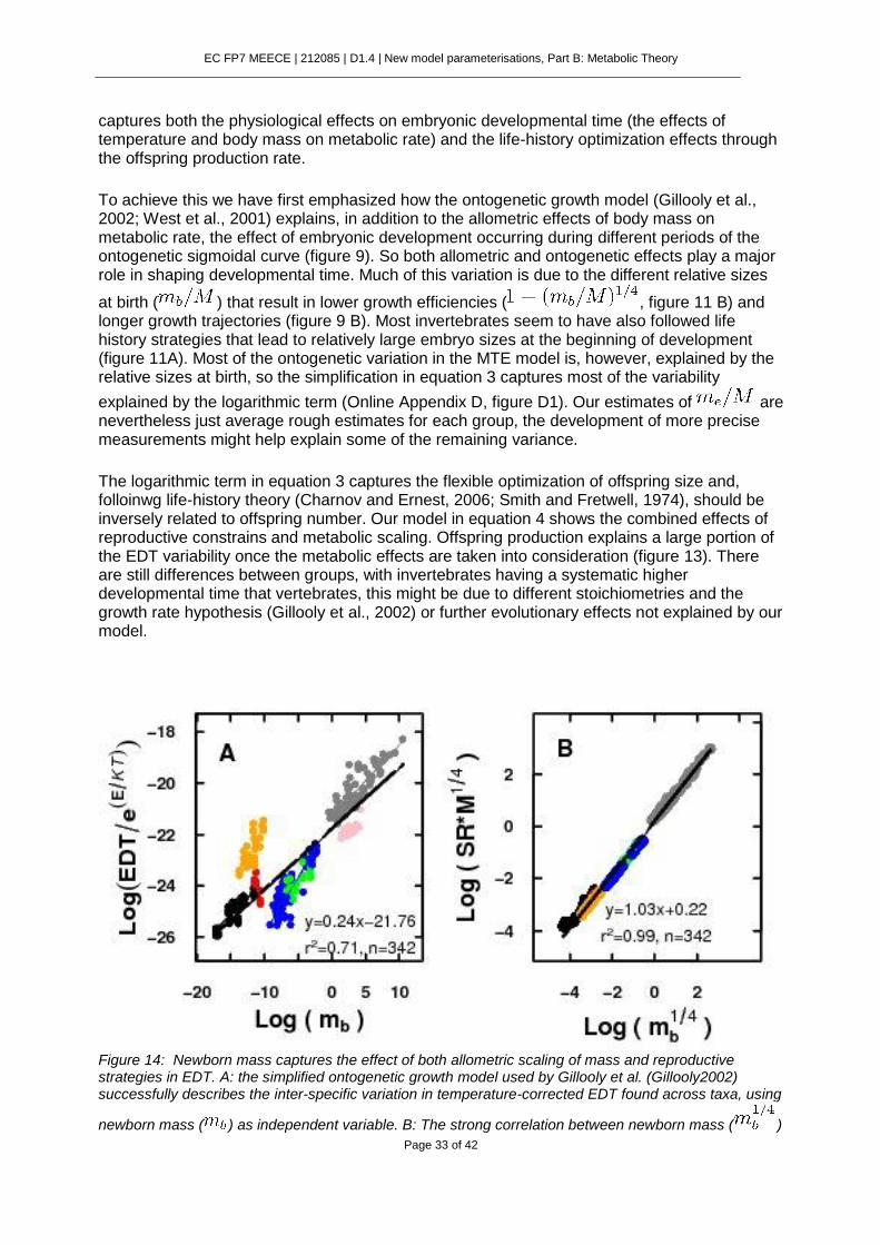
EC FP7 MEECE | 212085 | D1.4 | New model parameterisations, Part B: Metabolic Theory
Page 33 of 42
captures both the physiological effects on embryonic developmental time (the effects of temperature and body mass on metabolic rate) and the life-history optimization effects through the offspring production rate.
To achieve this we have first emphasized how the ontogenetic growth model (Gillooly et al., 2002; West et al., 2001) explains, in addition to the allometric effects of body mass on metabolic rate, the effect of embryonic development occurring during different periods of the ontogenetic sigmoidal curve (figure 9). So both allometric and ontogenetic effects play a major role in shaping developmental time. Much of this variation is due to the different relative sizes
at birth ( ) that result in lower growth efficiencies ( , figure 11 B) and longer growth trajectories (figure 9 B). Most invertebrates seem to have also followed life history strategies that lead to relatively large embryo sizes at the beginning of development (figure 11A). Most of the ontogenetic variation in the MTE model is, however, explained by the relative sizes at birth, so the simplification in equation 3 captures most of the variability
explained by the logarithmic term (Online Appendix D, figure D1). Our estimates of are nevertheless just average rough estimates for each group, the development of more precise measurements might help explain some of the remaining variance.
The logarithmic term in equation 3 captures the flexible optimization of offspring size and, folloinwg life-history theory (Charnov and Ernest, 2006; Smith and Fretwell, 1974), should be inversely related to offspring number. Our model in equation 4 shows the combined effects of reproductive constrains and metabolic scaling. Offspring production explains a large portion of the EDT variability once the metabolic effects are taken into consideration (figure 13). There are still differences between groups, with invertebrates having a systematic higher developmental time that vertebrates, this might be due to different stoichiometries and the growth rate hypothesis (Gillooly et al., 2002) or further evolutionary effects not explained by our model.
Figure 14: Newborn mass captures the effect of both allometric scaling of mass and reproductive strategies in EDT. A: the simplified ontogenetic growth model used by Gillooly et al. (Gillooly2002) successfully describes the inter-specific variation in temperature-corrected EDT found across taxa, using
newborn mass ( ) as independent variable. B: The strong correlation between newborn mass ( )
EC FP7 MEECE | 212085 | D1.4 | New model parameterisations, Part B: Metabolic Theory
Page 34 of 42
and the product of term and adult mass ( ) explains the usefulness of to incorporate both life-history and metabolic effects. Regression coefficients of each group in panel A in table C7.
But probably the most striking feature is how viviparous and oviparous species fall along the same mass and temperature corrected trade-off axis (figures 12 and 13). Charnov and Ernest (2006) model for mammals effectively showed that the resources available for reproduction are not constant between taxa and that normalization of offspring production rate by the allometric scaling of energy allocation with adult mass resulted in an inverse proportionality between offspring number and size. They also argued that their model could be probably applied to other taxa, something that we have tested with data for birds, fish, amphibians and invertebrates. The generality of the model is striking although some deviations exists, specially when using offspring body size at weaning and newborn size including yolk sacs (figure 12 B), a supposedly more precise measure of investment per offspring. This might reflect the extra error in estimating weaning mass (due to difficulties in the determination of the moment when weaning occurs) and yolk sac (that contains energy rich material) potential mass . But it could also be due to the lack of temperature normalization of offspring production rate in our analysis, which might be needed when comparing animals with very different body temperatures and hence rates of resource acquisition (Charnov and Ernest, 2006). We were unable to rigorously test these temperature effects on the offspring size - number trade-off due to the lack of appropriate data. Most studies on ectotherm fecundity do not provide simultaneous measures of adult and newborn mass (e.g. Hirst2003) hindering a precise validation. These temperature effects might explain the deviation of figure 12 B from the
predicted exponent, since offspring production of ectotherms might be lower because their body temperatures are usually lower than that of endotherms. But, as explained in the methods
section, we were unable to obtain concurrent measures of , and for most groups and we assigned mean values of brood sizes for each species for which we had developmental time information. But assuming that developmental temperature can be used as an approximate measure of maternal body temperature for ectotherms, and that adult mass and newborn mass are invariant with temperature (something not correct at least for marine ectotherms, Daufresne2009) we can assess the magnitude of this temperature effect, which
seems to explain part of the deviation from the predicted exponent (Online Appendix D;
figure D2). Experimental measures of concurrent , and are needed to further validate this pattern.
The integration of metabolic theory and life-history evolution can provide a synthetic theory of population energetics (Economo et al., 2005). Our model is a step in this direction and shows that both theories play a major role in controlling developmental time. Our view somehow contrasts with the Metabolic Theory of Ecology that argues that body size and temperature, through their effects on metabolic rates, control most biological rates and times (Brown et al., 2004; Gillooly et al., 2002; Savage et al., 2004). Gillooly et al. (2002) showed that newborn mass explained much of the variability in EDT, we believe this assertion is correct but for the wrong reason. Equation 1 is usually simplified by MTE theorists (Gillooly et al., 2002; Moses
et al., 2008) to on the basis that growth efficiency during embryo development is
maximal ( ), an approximation that we have shown to be mostly incorrect, with some groups showing growth efficiencies at birth close to 50% (figure 11 B). But, if this approximation is incorrect, why is Gillooly et al. (2002) model so successful in explaining EDT (figure 14 A) and higher order population and community rates? We believe this is simply
because is a good approximation to (figure 14B) and therefore captures in a single variable three effects all leading to longer developmental times: slower metabolism with increasing adult asymptotic size, lower growth efficiency with
EC FP7 MEECE | 212085 | D1.4 | New model parameterisations, Part B: Metabolic Theory
Page 35 of 42
increasing relative size at birth and longer ontogenetic growth trajectories with larger mass at birth. Gillooly et al. (2002) model is at the basis of many higher order predictions of MTE (Brown et al., 2004; Savage et al., 2004). Our analysis should reconcile LHO theorists with MTE as it shows that body mass effects include both metabolic scaling and life-history optimizations.
6.6 References
Brown, J. H., J. F. Gillooly, A. P. Allen, V. M. Savage, and G. B. West. 2004. Toward a metabolic theory of ecology. Ecology 85:1771–1789.
Charnov, E. L., and S. K. M. Ernest. 2006. The offspring-size/clutch-size trade-off in mammals. American Naturalist 167, 4:578–582.
Economo, E. P., A. J. Kerkhoff, and B. J. Enquist. 2005. Allometric growth, life-history invariants and population energetics. Ecology Letters 8:353–360.
Enquist, B. J., E. P. Economo, T. E. Huxman, A. P. Allen, D. D. Ignace, and J. F. Gillooly. 2003. Scaling metabolism from organisms to ecosystems. Nature 423:639–642.
Ernest, S. K. M. 2003. Life history characteristics of non-volant placental mammals. Ecology 84:3401.
Ernest, S. K. M., B. J. Enquist, J. H. Brown, E. L. Charnov, J. F. Gillooly, V. Savage, E. P. White, F. A. Smith, E. A. Hadly, J. P. Haskell, S. K. Lyons, B. A. Maurer, K. J. Niklas, and B. Tiffney. 2003. Thermodynamic and metabolic effects on the scaling of production and population energy use. Ecology Letters 6:990–995.
Gillooly, J. F., E. L. Charnov, G. B. West, V. M. Savage, and J. H. Brown. 2002. Effects of size and temperature on developmental time. Nature 417:70–73.
Harte, J. 2004. The value of null theories in ecology. Ecology 85:1792–1794.
Hirst, A., and A. Lopez-Urrutia. 2006. Effects of evolution on egg development time. Marine Ecology Progress Series 326:29–35.
Hou, C., W. Zuo, M. E. Moses, W. H. Woodruff, J. H. Brown, and G. B. West. 2008. Energy uptake and allocation during ontogeny. Science 322:736–739.
Kiørboe, T., and A. Hirst. 2008. Optimal development time in pelagic copepods. Marine Ecology Progress Series 367:15–22.
Makarieva, A. M., V. G. Gorshkov, and B. L. Li. 2009. Comment on "energy uptake and allocation during ontogeny". Science 325:1206.
Moses, M. E., C. Hou, W. H. Woodruff, G. B. West, J. C. Nekola, W. Zuo, and J. H. Brown. 2008. Revisiting a model of ontogenetic growth: Estimating model parameters from theory and data. American Naturalist 171:632–645.
O’Connor, M. I., S. J. Kemp, S. J. Agosta, F. Hansen, A. E. Sieg, B. P. Wallace, J. N. McNair, and A. E. Dunham. 2007. Reconsidering the mechanistic basis of the metabolic theory of ecology. Oikos 116:1058–1072.
Roff, D. 2002. Life History Evolution. Sinauer Associates, Inc., Sunderland, Massachusetts USA.

EC FP7 MEECE | 212085 | D1.4 | New model parameterisations, Part B: Metabolic Theory
Page 36 of 42
Savage, V. M., J. F. Gillooly, W. H. Woodruff, G. B. West, A. P. Allen, B. J. Enquist, and J. H. Brown. 2004. The predominance of quarter-power scaling in biology. Functional Ecology 18:257–282.
Sibly, R. M., and J. H. Brown. 2007. Effects of body size and lifestyle on evolution of mammal life histories. Proceedings of the National Academy of Sciences of the USA 104:17707–17712.
———. 2009. Mammal reproductive strategies driven by offspring mortality-size relationships. American Naturalist 173:185–199.
Smith, C. C., and S. D. Fretwell. 1974. The optimal balance between size and number of offspring. American Naturalist 108:499–506.
Sousa, T., G. M. Marques, and T. Domingos. 2009. Comment on "energy uptake and allocation during ontogeny". Science 325:1206b.
Stearns, S. C. 1992. The Evolution of Life Histories. Oxford Univ. Press, Oxford.
Visser, G. H., and A. J. Beintema. 1991. Reproductive characteristics of meadow birds and other European waders. Bulletin of the Wader Study Group 61:6–11.
West, G. B., J. H. Brown, and B. J. Enquist. 2001. A general model for ontogenetic growth. Nature 413:628–631.
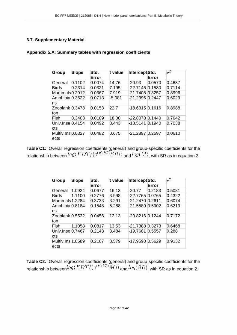
EC FP7 MEECE | 212085 | D1.4 | New model parameterisations, Part B: Metabolic Theory
Page 37 of 42
6.7. Supplementary Material.
Appendix 5.A: Summary tables with regression coefficients
Group Slope Std. Error
t value Intercept Std. Error
General 0.1102 0.0074 14.76 -20.93 0.0570 0.4637 Birds 0.2314 0.0321 7.195 -22.7145 0.1580 0.7114 Mammals 0.2912 0.0367 7.919 -21.7408 0.3257 0.8996 Amphibians
0.3622 0.0713 -5.081 -21.2396 0.2447 0.6029
Zooplankton
0.3478 0.0153 22.7 -18.6315 0.1616 0.8988
Fish 0.3408 0.0189 18.00 -22.8078 0.1440 0.7642 Univ.Insects
0.4154 0.0492 8.443 -18.5141 0.1940 0.7038
Multiv.Insects
0.0327 0.0482 0.675 -21.2897 0.2597 0.0610
Table C1: Overall regression coefficients (general) and group-specific coefficients for the
relationship between and , with SR as in equation 2. Table C2: Overall regression coefficients (general) and group-specific coefficients for the
relationship between and , with SR as in equation 2.
Group Slope Std. Error
t value Intercept Std. Error
General 1.0924 0.0677 16.13 -20.77 0.2183 0.5081 Birds 1.1100 0.2776 3.998 -22.7765 0.0765 0.4322 Mammals 1.2284 0.3733 3.291 -21.2470 0.2611 0.6074 Amphibians
0.8184 0.1548 5.288 -21.5589 0.5902 0.6219
Zooplankton
0.5532 0.0456 12.13 -20.8216 0.1244 0.7172
Fish 1.1058 0.0817 13.53 -21.7388 0.3273 0.6468 Univ.Insects
0.7467 0.2143 3.484 -19.7681 0.5557 0.288
Multiv.Insects
1.8589 0.2167 8.579 -17.9590 0.5629 0.9132
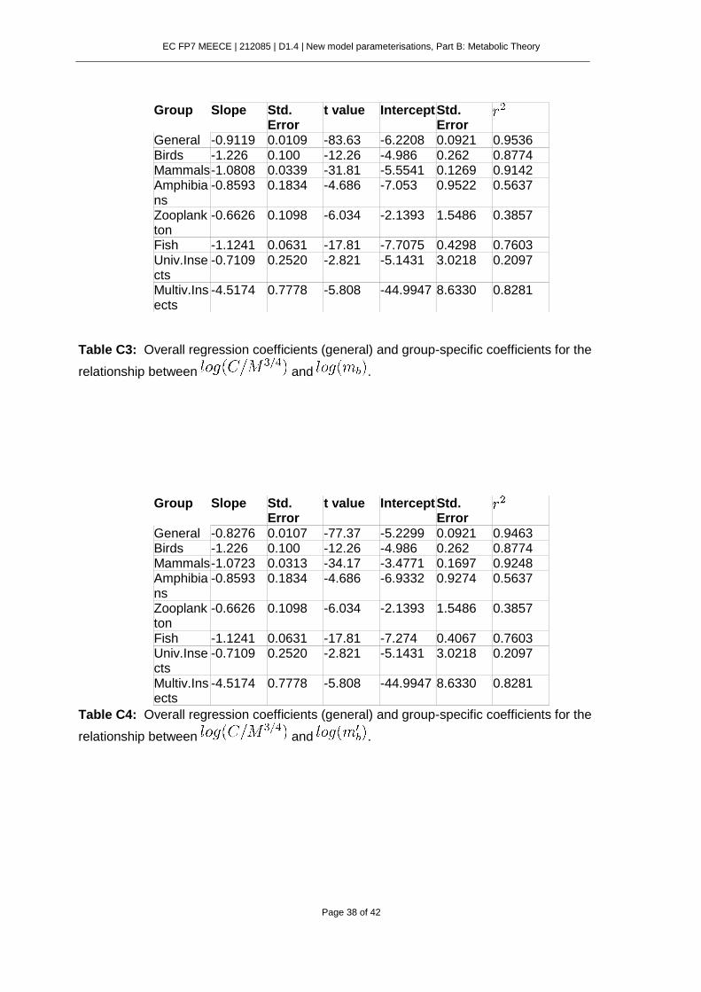
EC FP7 MEECE | 212085 | D1.4 | New model parameterisations, Part B: Metabolic Theory
Page 38 of 42
Table C3: Overall regression coefficients (general) and group-specific coefficients for the
relationship between and . Table C4: Overall regression coefficients (general) and group-specific coefficients for the
relationship between and .
Group Slope Std. Error
t value Intercept Std. Error
General -0.9119 0.0109 -83.63 -6.2208 0.0921 0.9536 Birds -1.226 0.100 -12.26 -4.986 0.262 0.8774 Mammals -1.0808 0.0339 -31.81 -5.5541 0.1269 0.9142 Amphibians
-0.8593 0.1834 -4.686 -7.053 0.9522 0.5637
Zooplankton
-0.6626 0.1098 -6.034 -2.1393 1.5486 0.3857
Fish -1.1241 0.0631 -17.81 -7.7075 0.4298 0.7603 Univ.Insects
-0.7109 0.2520 -2.821 -5.1431 3.0218 0.2097
Multiv.Insects
-4.5174 0.7778 -5.808 -44.9947 8.6330 0.8281
Group Slope Std. Error
t value Intercept Std. Error
General -0.8276 0.0107 -77.37 -5.2299 0.0921 0.9463 Birds -1.226 0.100 -12.26 -4.986 0.262 0.8774 Mammals -1.0723 0.0313 -34.17 -3.4771 0.1697 0.9248 Amphibians
-0.8593 0.1834 -4.686 -6.9332 0.9274 0.5637
Zooplankton
-0.6626 0.1098 -6.034 -2.1393 1.5486 0.3857
Fish -1.1241 0.0631 -17.81 -7.274 0.4067 0.7603 Univ.Insects
-0.7109 0.2520 -2.821 -5.1431 3.0218 0.2097
Multiv.Insects
-4.5174 0.7778 -5.808 -44.9947 8.6330 0.8281
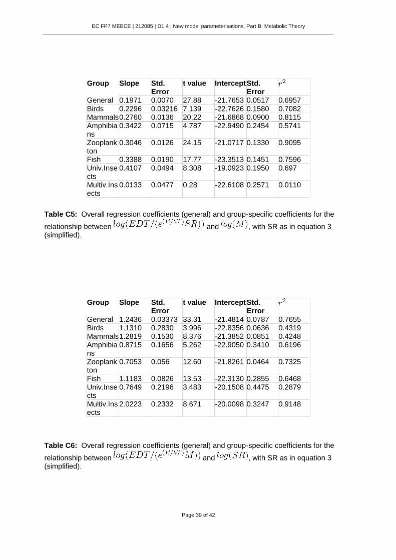
EC FP7 MEECE | 212085 | D1.4 | New model parameterisations, Part B: Metabolic Theory
Page 39 of 42
Table C5: Overall regression coefficients (general) and group-specific coefficients for the
relationship between and , with SR as in equation 3 (simplified). Table C6: Overall regression coefficients (general) and group-specific coefficients for the
relationship between and , with SR as in equation 3 (simplified).
Group Slope Std. Error
t value Intercept Std. Error
General 0.1971 0.0070 27.88 -21.7653 0.0517 0.6957 Birds 0.2296 0.03216 7.139 -22.7626 0.1580 0.7082 Mammals 0.2760 0.0136 20.22 -21.6868 0.0900 0.8115 Amphibians
0.3422 0.0715 4.787 -22.9490 0.2454 0.5741
Zooplankton
0.3046 0.0126 24.15 -21.0717 0.1330 0.9095
Fish 0.3388 0.0190 17.77 -23.3513 0.1451 0.7596 Univ.Insects
0.4107 0.0494 8.308 -19.0923 0.1950 0.697
Multiv.Insects
0.0133 0.0477 0.28 -22.6108 0.2571 0.0110
Group Slope Std. Error
t value Intercept Std. Error
General 1.2436 0.03373 33.31 -21.4814 0.0787 0.7655 Birds 1.1310 0.2830 3.996 -22.8356 0.0636 0.4319 Mammals 1.2819 0.1530 8.376 -21.3852 0.0851 0.4248 Amphibians
0.8715 0.1656 5.262 -22.9050 0.3410 0.6196
Zooplankton
0.7053 0.056 12.60 -21.8261 0.0464 0.7325
Fish 1.1183 0.0826 13.53 -22.3130 0.2855 0.6468 Univ.Insects
0.7649 0.2196 3.483 -20.1508 0.4475 0.2879
Multiv.Insects
2.0223 0.2332 8.671 -20.0098 0.3247 0.9148
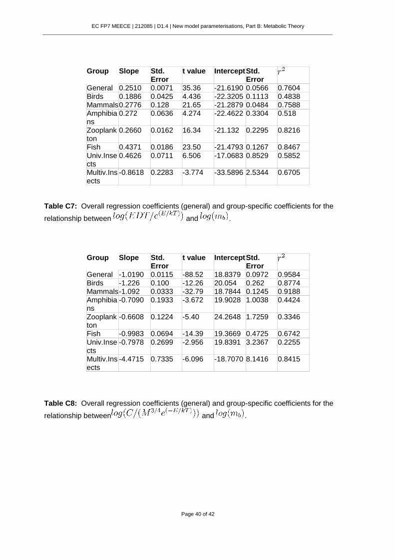
EC FP7 MEECE | 212085 | D1.4 | New model parameterisations, Part B: Metabolic Theory
Page 40 of 42
Group Slope Std. Error
t value Intercept Std. Error
General 0.2510 0.0071 35.36 -21.6190 0.0566 0.7604 Birds 0.1886 0.0425 4.436 -22.3205 0.1113 0.4838 Mammals 0.2776 0.128 21.65 -21.2879 0.0484 0.7588 Amphibians
0.272 0.0636 4.274 -22.4622 0.3304 0.518
Zooplankton
0.2660 0.0162 16.34 -21.132 0.2295 0.8216
Fish 0.4371 0.0186 23.50 -21.4793 0.1267 0.8467 Univ.Insects
0.4626 0.0711 6.506 -17.0683 0.8529 0.5852
Multiv.Insects
-0.8618 0.2283 -3.774 -33.5896 2.5344 0.6705
Table C7: Overall regression coefficients (general) and group-specific coefficients for the
relationship between and . Table C8: Overall regression coefficients (general) and group-specific coefficients for the
relationship between and .
Group Slope Std. Error
t value Intercept Std. Error
General -1.0190 0.0115 -88.52 18.8379 0.0972 0.9584 Birds -1.226 0.100 -12.26 20.054 0.262 0.8774 Mammals -1.092 0.0333 -32.79 18.7844 0.1245 0.9188 Amphibians
-0.7090 0.1933 -3.672 19.9028 1.0038 0.4424
Zooplankton
-0.6608 0.1224 -5.40 24.2648 1.7259 0.3346
Fish -0.9983 0.0694 -14.39 19.3669 0.4725 0.6742 Univ.Insects
-0.7978 0.2699 -2.956 19.8391 3.2367 0.2255
Multiv.Insects
-4.4715 0.7335 -6.096 -18.7070 8.1416 0.8415
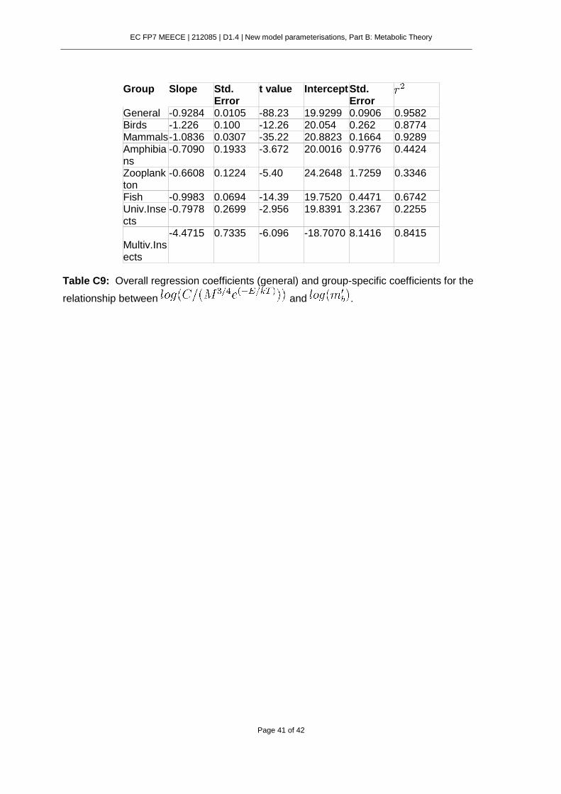
EC FP7 MEECE | 212085 | D1.4 | New model parameterisations, Part B: Metabolic Theory
Page 41 of 42
Group Slope Std.
Error t value Intercept Std.
Error
General -0.9284 0.0105 -88.23 19.9299 0.0906 0.9582 Birds -1.226 0.100 -12.26 20.054 0.262 0.8774 Mammals -1.0836 0.0307 -35.22 20.8823 0.1664 0.9289 Amphibians
-0.7090 0.1933 -3.672 20.0016 0.9776 0.4424
Zooplankton
-0.6608 0.1224 -5.40 24.2648 1.7259 0.3346
Fish -0.9983 0.0694 -14.39 19.7520 0.4471 0.6742 Univ.Insects
-0.7978 0.2699 -2.956 19.8391 3.2367 0.2255
Multiv.Insects
-4.4715 0.7335 -6.096 -18.7070 8.1416 0.8415
Table C9: Overall regression coefficients (general) and group-specific coefficients for the
relationship between and .

EC FP7 MEECE | 212085 | D1.4 | New model parameterisations, Part B: Metabolic Theory
Page 42 of 42
Appendix 5.B: Supporting figures
Figure D1: Same as figure 2 but using the simplified version of the from equation 3. Color legend as in figure 11. Regression coefficients in tables C5 and C6.
Figure D2: Same as Figure 4 but correcting offspring production by possible effects of temperature, see the main text for uncertainties in the determination of temperature at which offspring production was measured. Color legend as in fgure 11. Regression coefficients in tables C8 and C9.
Related Documents