3 SOLVING PROBLEMS BY SEARCHING In which we see how an agent can find a sequence of actions that achieves its goals, when no single action will do. The simplest agents discussed in Chapter 2 were the reflex agents, which base their actions on a direct mapping from states to actions. Such agents cannot operate well in environments for which this mapping would be too large to store and would take too long to learn. Goal-based agents, on the other hand, can succeed by considering future actions and the desirability of their outcomes. This chapter describes one kind of goal-based agent called a problem-solving agent. PROBLEM-SOLVING AGENT Problem-solving agents decide what to do by finding sequences of actions that lead to desir- able states. We start by defining precisely the elements that constitute a “problem” and its “solution,” and give several examples to illustrate these definitions. We then describe sev- eral general-purpose search algorithms that can be used to solve these problems and compare the advantages of each algorithm. The algorithms are uninformed, in the sense that they are given no information about the problem other than its definition. Chapter 4 deals with informed search algorithms, ones that have some idea of where to look for solutions. This chapter uses concepts from the analysis of algorithms. Readers unfamiliar with the concepts of asymptotic complexity (that is, O() notation) and NP-completeness should consult Appendix A. 3.1 P ROBLEM-S OLVING AGENTS Intelligent agents are supposed to maximize their performance measure. As we mentioned in Chapter 2, achieving this is sometimes simplified if the agent can adopt a goal and aim at satisfying it. Let us first look at why and how an agent might do this. Imagine an agent in the city of Arad, Romania, enjoying a touring holiday. The agent’s performance measure contains many factors: it wants to improve its suntan, improve its Ro- manian, take in the sights, enjoy the nightlife (such as it is), avoid hangovers, and so on. The decision problem is a complex one involving many tradeoffs and careful reading of guide- books. Now, suppose the agent has a nonrefundable ticket to fly out of Bucharest the follow- 59

Welcome message from author
This document is posted to help you gain knowledge. Please leave a comment to let me know what you think about it! Share it to your friends and learn new things together.
Transcript

3 SOLVING PROBLEMS BYSEARCHING
In which we see how an agent can find a sequence of actions that achieves itsgoals, when no single action will do.
The simplest agents discussed in Chapter 2 were the reflex agents, which base their actions ona direct mapping from states to actions. Such agents cannot operate well in environments forwhich this mapping would be too large to store and would take too long to learn. Goal-basedagents, on the other hand, can succeed by considering future actions and the desirability oftheir outcomes.
This chapter describes one kind of goal-based agent called a problem-solving agent.PROBLEM-SOLVINGAGENT
Problem-solving agents decide what to do by finding sequences of actions that lead to desir-able states. We start by defining precisely the elements that constitute a “problem” and its“solution,” and give several examples to illustrate these definitions. We then describe sev-eral general-purpose search algorithms that can be used to solve these problems and comparethe advantages of each algorithm. The algorithms are uninformed, in the sense that theyare given no information about the problem other than its definition. Chapter 4 deals withinformed search algorithms, ones that have some idea of where to look for solutions.
This chapter uses concepts from the analysis of algorithms. Readers unfamiliar withthe concepts of asymptotic complexity (that is, O() notation) and NP-completeness shouldconsult Appendix A.
3.1 PROBLEM-SOLVING AGENTS
Intelligent agents are supposed to maximize their performance measure. As we mentionedin Chapter 2, achieving this is sometimes simplified if the agent can adopt a goal and aim atsatisfying it. Let us first look at why and how an agent might do this.
Imagine an agent in the city of Arad, Romania, enjoying a touring holiday. The agent’sperformance measure contains many factors: it wants to improve its suntan, improve its Ro-manian, take in the sights, enjoy the nightlife (such as it is), avoid hangovers, and so on. Thedecision problem is a complex one involving many tradeoffs and careful reading of guide-books. Now, suppose the agent has a nonrefundable ticket to fly out of Bucharest the follow-
59

60 Chapter 3. Solving Problems by Searching
ing day. In that case, it makes sense for the agent to adopt the goal of getting to Bucharest.Courses of action that don’t reach Bucharest on time can be rejected without further consid-eration and the agent’s decision problem is greatly simplified. Goals help organize behaviorby limiting the objectives that the agent is trying to achieve. Goal formulation, based on theGOAL FORMULATION
current situation and the agent’s performance measure, is the first step in problem solving.We will consider a goal to be a set of world states—exactly those states in which the
goal is satisfied. The agent’s task is to find out which sequence of actions will get it to a goalstate. Before it can do this, it needs to decide what sorts of actions and states to consider. If itwere to try to consider actions at the level of “move the left foot forward an inch” or “turn thesteering wheel one degree left,” the agent would probably never find its way out of the parkinglot, let alone to Bucharest, because at that level of detail there is too much uncertainty in theworld and there would be too many steps in a solution. Problem formulation is the processPROBLEM
FORMULATION
of deciding what actions and states to consider, given a goal. We will discuss this process inmore detail later. For now, let us assume that the agent will consider actions at the level ofdriving from one major town to another. The states it will consider therefore correspond tobeing in a particular town.1
Our agent has now adopted the goal of driving to Bucharest, and is considering whereto go from Arad. There are three roads out of Arad, one toward Sibiu, one to Timisoara, andone to Zerind. None of these achieves the goal, so unless the agent is very familiar with thegeography of Romania, it will not know which road to follow.2 In other words, the agent willnot know which of its possible actions is best, because it does not know enough about thestate that results from taking each action. If the agent has no additional knowledge, then it isstuck. The best it can do is choose one of the actions at random.
But suppose the agent has a map of Romania, either on paper or in its memory. Thepoint of a map is to provide the agent with information about the states it might get itselfinto, and the actions it can take. The agent can use this information to consider subsequentstages of a hypothetical journey via each of the three towns, trying to find a journey thateventually gets to Bucharest. Once it has found a path on the map from Arad to Bucharest,it can achieve its goal by carrying out the driving actions that correspond to the legs of thejourney. In general, an agent with several immediate options of unknown value can decidewhat to do by first examining different possible sequences of actions that lead to states ofknown value, and then choosing the best sequence.
This process of looking for such a sequence is called search. A search algorithm takes aSEARCH
problem as input and returns a solution in the form of an action sequence. Once a solution isSOLUTION
found, the actions it recommends can be carried out. This is called the execution phase. Thus,EXECUTION
we have a simple “formulate, search, execute” design for the agent, as shown in Figure 3.1.After formulating a goal and a problem to solve, the agent calls a search procedure to solveit. It then uses the solution to guide its actions, doing whatever the solution recommends as
1 Notice that each of these “states” actually corresponds to a large set of world states, because a real world statespecifies every aspect of reality. It is important to keep in mind the distinction between states in problem solvingand world states.2 We are assuming that most readers are in the same position and can easily imagine themselves to be as cluelessas our agent. We apologize to Romanian readers who are unable to take advantage of this pedagogical device.

Section 3.1. Problem-Solving Agents 61
function SIMPLE-PROBLEM-SOLVING-AGENT(percept) returns an actioninputs: percept , a perceptstatic: seq , an action sequence, initially empty
state , some description of the current world stategoal , a goal, initially nullproblem , a problem formulation
state←UPDATE-STATE(state ,percept)if seq is empty then do
goal← FORMULATE-GOAL(state)problem← FORMULATE-PROBLEM(state , goal)seq← SEARCH(problem)
action← FIRST(seq)seq←REST(seq)return action
Figure 3.1 A simple problem-solving agent. It first formulates a goal and a problem,searches for a sequence of actions that would solve the problem, and then executes the actionsone at a time. When this is complete, it formulates another goal and starts over. Note thatwhen it is executing the sequence it ignores its percepts: it assumes that the solution it hasfound will always work.
the next thing to do—typically, the first action of the sequence—and then removing that stepfrom the sequence. Once the solution has been executed, the agent will formulate a new goal.
We first describe the process of problem formulation, and then devote the bulk of thechapter to various algorithms for the SEARCH function. We will not discuss the workings ofthe UPDATE-STATE and FORMULATE-GOAL functions further in this chapter.
Before plunging into the details, let us pause briefly to see where problem-solvingagents fit into the discussion of agents and environments in Chapter 2. The agent designin Figure 3.1 assumes that the environment is static, because formulating and solving theproblem is done without paying attention to any changes that might be occurring in the envi-ronment. The agent design also assumes that the initial state is known; knowing it is easiestif the environment is observable. The idea of enumerating “alternative courses of action”assumes that the environment can be viewed as discrete. Finally, and most importantly, theagent design assumes that the environment is deterministic. Solutions to problems are singlesequences of actions, so they cannot handle any unexpected events; moreover, solutions areexecuted without paying attention to the percepts! An agent that carries out its plans with itseyes closed, so to speak, must be quite certain of what is going on. (Control theorists callthis an open-loop system, because ignoring the percepts breaks the loop between agent andOPEN-LOOP
environment.) All these assumptions mean that we are dealing with the easiest kinds of en-vironments, which is one reason this chapter comes early on in the book. Section 3.6 takes abrief look at what happens when we relax the assumptions of observability and determinism.Chapters 12 and 17 go into much greater depth.

62 Chapter 3. Solving Problems by Searching
Well-defined problems and solutions
A problem can be defined formally by four components:PROBLEM
• The initial state that the agent starts in. For example, the initial state for our agent inINITIAL STATE
Romania might be described as In(Arad).
• A description of the possible actions available to the agent. The most common for-mulation3 uses a successor function. Given a particular state x, SUCCESSOR-FN(x)SUCCESSOR
FUNCTION
returns a set of 〈action, successor〉 ordered pairs, where each action is one of the legalactions in state x and each successor is a state that can be reached from x by applyingthe action. For example, from the state In(Arad), the successor function for the Roma-nia problem would return
{〈Go(Sibiu), In(Sibiu)〉, 〈Go(Timisoara), In(Timisoara)〉, 〈Go(Zerind), In(Zerind)〉}Together, the initial state and successor function implicitly define the state space of theSTATE SPACE
problem—the set of all states reachable from the initial state. The state space forms agraph in which the nodes are states and the arcs between nodes are actions. (The mapof Romania shown in Figure 3.2 can be interpreted as a state space graph if we vieweach road as standing for two driving actions, one in each direction.) A path in the statePATH
space is a sequence of states connected by a sequence of actions.
• The goal test, which determines whether a given state is a goal state. Sometimes thereGOAL TEST
is an explicit set of possible goal states, and the test simply checks whether the givenstate is one of them. The agent’s goal in Romania is the singleton set {In(Bucharest)}.Sometimes the goal is specified by an abstract property rather than an explicitly enumer-ated set of states. For example, in chess, the goal is to reach a state called “checkmate,”where the opponent’s king is under attack and can’t escape.
• A path cost function that assigns a numeric cost to each path. The problem-solvingPATH COST
agent chooses a cost function that reflects its own performance measure. For the agenttrying to get to Bucharest, time is of the essence, so the cost of a path might be its lengthin kilometers. In this chapter, we assume that the cost of a path can be described as thesum of the costs of the individual actions along the path. The step cost of taking actionSTEP COST
a to go from state x to state y is denoted by c(x, a, y). The step costs for Romania areshown in Figure 3.2 as route distances. We will assume that step costs are nonnegative.4
The preceding elements define a problem and can be gathered together into a single datastructure that is given as input to a problem-solving algorithm. A solution to a problem isa path from the initial state to a goal state. Solution quality is measured by the path costfunction, and an optimal solution has the lowest path cost among all solutions.OPTIMAL SOLUTION
Formulating problems
In the preceding section we proposed a formulation of the problem of getting to Bucharest interms of the initial state, successor function, goal test, and path cost. This formulation seems
3 An alternative formulation uses a set of operators that can be applied to a state to generate successors.4 The implications of negative costs are explored in Exercise 3.17.

Section 3.1. Problem-Solving Agents 63
Giurgiu
UrziceniHirsova
Eforie
Neamt
Oradea
Zerind
Arad
Timisoara
Lugoj
Mehadia
Dobreta
Craiova
Sibiu Fagaras
Pitesti
Vaslui
Iasi
Rimnicu Vilcea
Bucharest
71
75
118
111
70
75
120
151
140
99
80
97
101
211
138
146 85
90
98
142
92
87
86
Figure 3.2 A simplified road map of part of Romania.
reasonable, yet it omits a great many aspects of the real world. Compare the simple statedescription we have chosen, In(Arad), to an actual cross-country trip, where the state of theworld includes so many things: the traveling companions, what is on the radio, the sceneryout of the window, whether there are any law enforcement officers nearby, how far it is to thenext rest stop, the condition of the road, the weather, and so on. All these considerations areleft out of our state descriptions because they are irrelevant to the problem of finding a routeto Bucharest. The process of removing detail from a representation is called abstraction.ABSTRACTION
In addition to abstracting the state description, we must abstract the actions themselves.A driving action has many effects. Besides changing the location of the vehicle and its occu-pants, it takes up time, consumes fuel, generates pollution, and changes the agent (as they say,travel is broadening). In our formulation, we take into account only the change in location.Also, there are many actions that we will omit altogether: turning on the radio, looking out ofthe window, slowing down for law enforcement officers, and so on. And of course, we don’tspecify actions at the level of “turn steering wheel to the left by three degrees.”
Can we be more precise about defining the appropriate level of abstraction? Think of theabstract states and actions we have chosen as corresponding to large sets of detailed worldstates and detailed action sequences. Now consider a solution to the abstract problem: forexample, the path from Arad to Sibiu to Rimnicu Vilcea to Pitesti to Bucharest. This abstractsolution corresponds to a large number of more detailed paths. For example, we could drivewith the radio on between Sibiu and Rimnicu Vilcea, and then switch it off for the rest ofthe trip. The abstraction is valid if we can expand any abstract solution into a solution in themore detailed world; a sufficient condition is that for every detailed state that is “in Arad,”

64 Chapter 3. Solving Problems by Searching
there is a detailed path to some state that is “in Sibiu,” and so on. The abstraction is usefulif carrying out each of the actions in the solution is easier than the original problem; in thiscase they are easy enough that they can be carried out without further search or planning byan average driving agent. The choice of a good abstraction thus involves removing as muchdetail as possible while retaining validity and ensuring that the abstract actions are easy tocarry out. Were it not for the ability to construct useful abstractions, intelligent agents wouldbe completely swamped by the real world.
3.2 EXAMPLE PROBLEMS
The problem-solving approach has been applied to a vast array of task environments. Welist some of the best known here, distinguishing between toy and real-world problems. A toyproblem is intended to illustrate or exercise various problem-solving methods. It can be givenTOY PROBLEM
a concise, exact description. This means that it can be used easily by different researchersto compare the performance of algorithms. A real-world problem is one whose solutionsREAL-WORLD
PROBLEM
people actually care about. They tend not to have a single agreed-upon description, but wewill attempt to give the general flavor of their formulations.
Toy problems
The first example we will examine is the vacuum world first introduced in Chapter 2. (SeeFigure 2.2.) This can be formulated as a problem as follows:
♦ States: The agent is in one of two locations, each of which might or might not containdirt. Thus there are 2× 22 = 8 possible world states.
♦ Initial state: Any state can be designated as the initial state.
♦ Successor function: This generates the legal states that result from trying the threeactions (Left, Right, and Suck). The complete state space is shown in Figure 3.3.
♦ Goal test: This checks whether all the squares are clean.
♦ Path cost: Each step costs 1, so the path cost is the number of steps in the path.
Compared with the real world, this toy problem has discrete locations, discrete dirt, reliablecleaning, and it never gets messed up once cleaned. (In Section 3.6, we will relax theseassumptions.) One important thing to note is that the state is determined by both the agentlocation and the dirt locations. A larger environment with n locations has n 2n states.
The 8-puzzle, an instance of which is shown in Figure 3.4, consists of a 3×3 board with8-PUZZLE
eight numbered tiles and a blank space. A tile adjacent to the blank space can slide into thespace. The object is to reach a specified goal state, such as the one shown on the right of thefigure. The standard formulation is as follows:
♦ States: A state description specifies the location of each of the eight tiles and the blankin one of the nine squares.
♦ Initial state: Any state can be designated as the initial state. Note that any given goalcan be reached from exactly half of the possible initial states (Exercise 3.4).

Section 3.2. Example Problems 65
R
L
S S
S S
R
L
R
L
R
L
S
SS
S
L
L
LL R
R
R
R
Figure 3.3 The state space for the vacuum world. Arcs denote actions: L = Left, R =Right, S = Suck.
♦ Successor function: This generates the legal states that result from trying the fouractions (blank moves Left, Right, Up, or Down).
♦ Goal test: This checks whether the state matches the goal configuration shown in Fig-ure 3.4. (Other goal configurations are possible.)
♦ Path cost: Each step costs 1, so the path cost is the number of steps in the path.
What abstractions have we included here? The actions are abstracted to their begin-ning and final states, ignoring the intermediate locations where the block is sliding. We’veabstracted away actions such as shaking the board when pieces get stuck, or extracting thepieces with a knife and putting them back again. We’re left with a description of the rules ofthe puzzle, avoiding all the details of physical manipulations.
2
Start State Goal State
1
3 4
6 7
5
1
2
3
4
6
7
8
5
8
Figure 3.4 A typical instance of the 8-puzzle.

66 Chapter 3. Solving Problems by Searching
The 8-puzzle belongs to the family of sliding-block puzzles, which are often used asSLIDING-BLOCKPUZZLES
test problems for new search algorithms in AI. This general class is known to be NP-complete,so one does not expect to find methods significantly better in the worst case than the searchalgorithms described in this chapter and the next. The 8-puzzle has 9!/2=181, 440 reachablestates and is easily solved. The 15-puzzle (on a 4×4 board) has around 1.3 trillion states, andrandom instances can be solved optimally in a few milliseconds by the best search algorithms.The 24-puzzle (on a 5× 5 board) has around 1025 states, and random instances are still quitedifficult to solve optimally with current machines and algorithms.
The goal of the 8-queens problem is to place eight queens on a chessboard such that8-QUEENS PROBLEM
no queen attacks any other. (A queen attacks any piece in the same row, column or diago-nal.) Figure 3.5 shows an attempted solution that fails: the queen in the rightmost column isattacked by the queen at the top left.
Figure 3.5 Almost a solution to the 8-queens problem. (Solution is left as an exercise.)
Although efficient special-purpose algorithms exist for this problem and the whole n-queens family, it remains an interesting test problem for search algorithms. There are twomain kinds of formulation. An incremental formulation involves operators that augmentINCREMENTAL
FORMULATION
the state description, starting with an empty state; for the 8-queens problem, this means thateach action adds a queen to the state. A complete-state formulation starts with all 8 queensCOMPLETE-STATE
FORMULATION
on the board and moves them around. In either case, the path cost is of no interest becauseonly the final state counts. The first incremental formulation one might try is the following:
♦ States: Any arrangement of 0 to 8 queens on the board is a state.
♦ Initial state: No queens on the board.
♦ Successor function: Add a queen to any empty square.
♦ Goal test: 8 queens are on the board, none attacked.

Section 3.2. Example Problems 67
In this formulation, we have 64 · 63 · · · 57 ≈ 3× 10¹⁴ possible sequences to investigate. Abetter formulation would prohibit placing a queen in any square that is already attacked:
♦ States: Arrangements of n queens (0 ≤ n ≤ 8), one per column in the leftmost ncolumns, with no queen attacking another are states.
♦ Successor function: Add a queen to any square in the leftmost empty column such thatit is not attacked by any other queen.
This formulation reduces the 8-queens state space from 3× 10¹⁴ to just 2,057, and solutionsare easy to find. On the other hand, for 100 queens the initial formulation has roughly 10400
states whereas the improved formulation has about 1052 states (Exercise 3.5). This is a hugereduction, but the improved state space is still too big for the algorithms in this chapter tohandle. Chapter 4 describes the complete-state formulation and Chapter 5 gives a simplealgorithm that makes even the million-queens problem easy to solve.
Real-world problems
We have already seen how the route-finding problem is defined in terms of specified loca-ROUTE-FINDINGPROBLEM
tions and transitions along links between them. Route-finding algorithms are used in a varietyof applications, such as routing in computer networks, military operations planning, and air-line travel planning systems. These problems are typically complex to specify. Consider asimplified example of an airline travel problem specified as follows:
♦ States: Each is represented by a location (e.g., an airport) and the current time.♦ Initial state: This is specified by the problem.
♦ Successor function: This returns the states resulting from taking any scheduled flight(perhaps further specified by seat class and location), leaving later than the current timeplus the within-airport transit time, from the current airport to another.
♦ Goal test: Are we at the destination by some prespecified time?
♦ Path cost: This depends on monetary cost, waiting time, flight time, customs and im-migration procedures, seat quality, time of day, type of airplane, frequent-flyer mileageawards, and so on.
Commercial travel advice systems use a problem formulation of this kind, with many addi-tional complications to handle the byzantine fare structures that airlines impose. Any sea-soned traveller knows, however, that not all air travel goes according to plan. A really goodsystem should include contingency plans—such as backup reservations on alternate flights—to the extent that these are justified by the cost and likelihood of failure of the original plan.
Touring problems are closely related to route-finding problems, but with an importantTOURING PROBLEMS
difference. Consider, for example, the problem, “Visit every city in Figure 3.2 at least once,starting and ending in Bucharest.” As with route finding, the actions correspond to tripsbetween adjacent cities. The state space, however, is quite different. Each state must includenot just the current location but also the set of cities the agent has visited. So the initialstate would be “In Bucharest; visited {Bucharest},” a typical intermediate state would be “InVaslui; visited {Bucharest,Urziceni,Vaslui},” and the goal test would check whether the agentis in Bucharest and all 20 cities have been visited.

68 Chapter 3. Solving Problems by Searching
The traveling salesperson problem (TSP) is a touring problem in which each cityTRAVELINGSALESPERSONPROBLEM
must be visited exactly once. The aim is to find the shortest tour. The problem is known tobe NP-hard, but an enormous amount of effort has been expended to improve the capabilitiesof TSP algorithms. In addition to planning trips for traveling salespersons, these algorithmshave been used for tasks such as planning movements of automatic circuit-board drills and ofstocking machines on shop floors.
A VLSI layout problem requires positioning millions of components and connectionsVLSI LAYOUT
on a chip to minimize area, minimize circuit delays, minimize stray capacitances, and max-imize manufacturing yield. The layout problem comes after the logical design phase, and isusually split into two parts: cell layout and channel routing. In cell layout, the primitivecomponents of the circuit are grouped into cells, each of which performs some recognizedfunction. Each cell has a fixed footprint (size and shape) and requires a certain number ofconnections to each of the other cells. The aim is to place the cells on the chip so that theydo not overlap and so that there is room for the connecting wires to be placed between thecells. Channel routing finds a specific route for each wire through the gaps between the cells.These search problems are extremely complex, but definitely worth solving. In Chapter 4, wewill see some algorithms capable of solving them.
Robot navigation is a generalization of the route-finding problem described earlier.ROBOT NAVIGATION
Rather than a discrete set of routes, a robot can move in a continuous space with (in principle)an infinite set of possible actions and states. For a circular robot moving on a flat surface,the space is essentially two-dimensional. When the robot has arms and legs or wheels thatmust also be controlled, the search space becomes many-dimensional. Advanced techniquesare required just to make the search space finite. We examine some of these methods inChapter 25. In addition to the complexity of the problem, real robots must also deal witherrors in their sensor readings and motor controls.
Automatic assembly sequencing of complex objects by a robot was first demonstratedAUTOMATICASSEMBLYSEQUENCING
by FREDDY (Michie, 1972). Progress since then has been slow but sure, to the point wherethe assembly of intricate objects such as electric motors is economically feasible. In assemblyproblems, the aim is to find an order in which to assemble the parts of some object. If thewrong order is chosen, there will be no way to add some part later in the sequence withoutundoing some of the work already done. Checking a step in the sequence for feasibility is adifficult geometrical search problem closely related to robot navigation. Thus, the generationof legal successors is the expensive part of assembly sequencing. Any practical algorithmmust avoid exploring all but a tiny fraction of the state space. Another important assemblyproblem is protein design, in which the goal is to find a sequence of amino acids that willPROTEIN DESIGN
fold into a three-dimensional protein with the right properties to cure some disease.In recent years there has been increased demand for software robots that perform In-
ternet searching, looking for answers to questions, for related information, or for shoppingINTERNETSEARCHING
deals. This is a good application for search techniques, because it is easy to conceptualize theInternet as a graph of nodes (pages) connected by links. A full description of Internet searchis deferred until Chapter 10.

Section 3.3. Searching for Solutions 69
3.3 SEARCHING FOR SOLUTIONS
Having formulated some problems, we now need to solve them. This is done by a searchthrough the state space. This chapter deals with search techniques that use an explicit searchtree that is generated by the initial state and the successor function that together define theSEARCH TREE
state space. In general, we may have a search graph rather than a search tree, when thesame state can be reached from multiple paths. We defer consideration of this importantcomplication until Section 3.5.
Figure 3.6 shows some of the expansions in the search tree for finding a route fromArad to Bucharest. The root of the search tree is a search node corresponding to the initialSEARCH NODE
state, In(Arad). The first step is to test whether this is a goal state. Clearly it is not, butit is important to check so that we can solve trick problems like “starting in Arad, get toArad.” Because this is not a goal state, we need to consider some other states. This is doneby expanding the current state; that is, applying the successor function to the current state,EXPANDING
thereby generating a new set of states. In this case, we get three new states: In(Sibiu),GENERATING
In(Timisoara), and In(Zerind). Now we must choose which of these three possibilities toconsider further.
This is the essence of search—following up one option now and putting the others asidefor later, in case the first choice does not lead to a solution. Suppose we choose Sibiu first.We check to see whether it is a goal state (it is not) and then expand it to get In(Arad),In(Fagaras), In(Oradea), and In(RimnicuVilcea). We can then choose any of these four, orgo back and choose Timisoara or Zerind. We continue choosing, testing, and expanding untileither a solution is found or there are no more states to be expanded. The choice of whichstate to expand is determined by the search strategy. The general tree-search algorithm isSEARCH STRATEGY
described informally in Figure 3.7.It is important to distinguish between the state space and the search tree. For the route
finding problem, there are only 20 states in the state space, one for each city. But there arean infinite number of paths in this state space, so the search tree has an infinite number ofnodes. For example, the three paths Arad–Sibiu, Arad–Sibiu–Arad, Arad–Sibiu–Arad–Sibiuare the first three of an infinite sequence of paths. (Obviously, a good search algorithm avoidsfollowing such repeated paths; Section 3.5 shows how.)
There are many ways to represent nodes, but we will assume that a node is a datastructure with five components:
• STATE: the state in the state space to which the node corresponds;• PARENT-NODE: the node in the search tree that generated this node;• ACTION: the action that was applied to the parent to generate the node;• PATH-COST: the cost, traditionally denoted by g(n), of the path from the initial state to
the node, as indicated by the parent pointers; and• DEPTH: the number of steps along the path from the initial state.
It is important to remember the distinction between nodes and states. A node is a bookkeepingdata structure used to represent the search tree. A state corresponds to a configuration of the

70 Chapter 3. Solving Problems by Searching
world. Thus, nodes are on particular paths, as defined by PARENT-NODE pointers, whereasstates are not. Furthermore, two different nodes can contain the same world state, if that stateis generated via two different search paths. The node data structure is depicted in Figure 3.8.
We also need to represent the collection of nodes that have been generated but not yetexpanded—this collection is called the fringe. Each element of the fringe is a leaf node, thatFRINGE
LEAF NODE
(a) The initial state
(b) After expanding Arad
(c) After expanding Sibiu
Rimnicu Vilcea LugojArad Fagaras Oradea AradArad Oradea
Rimnicu Vilcea Lugoj
ZerindSibiu
Arad Fagaras Oradea
Timisoara
AradArad Oradea
Lugoj AradArad Oradea
Zerind
Arad
Sibiu Timisoara
Arad
Rimnicu Vilcea
Zerind
Arad
Sibiu
Arad Fagaras Oradea
Timisoara
Figure 3.6 Partial search trees for finding a route from Arad to Bucharest. Nodes thathave been expanded are shaded; nodes that have been generated but not yet expanded areoutlined in bold; nodes that have not yet been generated are shown in faint dashed lines.
function TREE-SEARCH(problem, strategy) returns a solution, or failureinitialize the search tree using the initial state of problem
loop doif there are no candidates for expansion then return failurechoose a leaf node for expansion according to strategy
if the node contains a goal state then return the corresponding solutionelse expand the node and add the resulting nodes to the search tree
Figure 3.7 An informal description of the general tree-search algorithm.

Section 3.3. Searching for Solutions 71
1
23
45
6
7
81
23
45
6
7
8
NodeDEPTH = 6
STATE
PARENT-NODE
ACTION = right
PATH-COST = 6
Figure 3.8 Nodes are the data structures from which the search tree is constructed. Eachhas a parent, a state, and various bookkeeping fields. Arrows point from child to parent.
is, a node with no successors in the tree. In Figure 3.6, the fringe of each tree consists of thosenodes with bold outlines. The simplest representation of the fringe would be a set of nodes.The search strategy then would be a function that selects the next node to be expanded fromthis set. Although this is conceptually straightforward, it could be computationally expensive,because the strategy function might have to look at every element of the set to choose the bestone. Therefore, we will assume that the collection of nodes is implemented as a queue. TheQUEUE
operations on a queue are as follows:
• MAKE-QUEUE(element , . . . ) creates a queue with the given element(s).
• EMPTY?(queue) returns true only if there are no more elements in the queue.
• FIRST(queue) returns the first element of the queue.
• REMOVE-FIRST(queue) returns FIRST(queue) and removes it from the queue.
• INSERT(element , queue) inserts an element into the queue and returns the resultingqueue. (We will see that different types of queues insert elements in different orders.)
• INSERT-ALL(elements , queue) inserts a set of elements into the queue and returns theresulting queue.
With these definitions, we can write the more formal version of the general tree-search algo-rithm shown in Figure 3.9.
Measuring problem-solving performance
The output of a problem-solving algorithm is either failure or a solution. (Some algorithmsmight get stuck in an infinite loop and never return an output.) We will evaluate an algorithm’sperformance in four ways:
♦ Completeness: Is the algorithm guaranteed to find a solution when there is one?COMPLETENESS
♦ Optimality: Does the strategy find the optimal solution, as defined on page 62?OPTIMALITY
♦ Time complexity: How long does it take to find a solution?TIME COMPLEXITY
♦ Space complexity: How much memory is needed to perform the search?SPACE COMPLEXITY

72 Chapter 3. Solving Problems by Searching
function TREE-SEARCH(problem, fringe) returns a solution, or failure
fringe← INSERT(MAKE-NODE(INITIAL-STATE[problem]), fringe)loop do
if EMPTY?( fringe) then return failurenode←REMOVE-FIRST( fringe)if GOAL-TEST[problem] applied to STATE[node] succeeds
then return SOLUTION(node)fringe← INSERT-ALL(EXPAND(node ,problem), fringe)
function EXPAND(node,problem) returns a set of nodes
successors← the empty setfor each 〈action , result〉 in SUCCESSOR-FN[problem](STATE[node]) do
s← a new NODE
STATE[s]← result
PARENT-NODE[s]←node
ACTION[s]← action
PATH-COST[s]← PATH-COST[node] + STEP-COST(node,action , s)DEPTH[s]←DEPTH[node] + 1add s to successors
return successors
Figure 3.9 The general tree-search algorithm. (Note that the fringe argument must be anempty queue, and the type of the queue will affect the order of the search.) The SOLUTION
function returns the sequence of actions obtained by following parent pointers back to theroot.
Time and space complexity are always considered with respect to some measure of the prob-lem difficulty. In theoretical computer science, the typical measure is the size of the statespace graph, because the graph is viewed as an explicit data structure that is input to thesearch program. (The map of Romania is an example of this.) In AI, where the graph isrepresented implicitly by the initial state and successor function and is frequently infinite,complexity is expressed in terms of three quantities: b, the branching factor or maximumBRANCHING FACTOR
number of successors of any node; d, the depth of the shallowest goal node; and m, themaximum length of any path in the state space.
Time is often measured in terms of the number of nodes generated5 during the search,and space in terms of the maximum number of nodes stored in memory.
To assess the effectiveness of a search algorithm, we can consider just the search cost—SEARCH COST
which typically depends on the time complexity but can also include a term for memoryusage—or we can use the total cost, which combines the search cost and the path cost of theTOTAL COST
solution found. For the problem of finding a route from Arad to Bucharest, the search cost
5 Some texts measure time in terms of the number of node expansions instead. The two measures differ by atmost a factor of b. It seems to us that the execution time of a node expansion increases with the number of nodesgenerated in that expansion.

Section 3.4. Uninformed Search Strategies 73
is the amount of time taken by the search and the solution cost is the total length of the pathin kilometers. Thus, to compute the total cost, we have to add kilometers and milliseconds.There is no “official exchange rate” between the two, but it might be reasonable in this case toconvert kilometers into milliseconds by using an estimate of the car’s average speed (becausetime is what the agent cares about). This enables the agent to find an optimal tradeoff pointat which further computation to find a shorter path becomes counterproductive. The moregeneral problem of tradeoffs between different goods will be taken up in Chapter 16.
3.4 UNINFORMED SEARCH STRATEGIES
This section covers five search strategies that come under the heading of uninformed searchUNINFORMEDSEARCH
(also called blind search). The term means that they have no additional information aboutstates beyond that provided in the problem definition. All they can do is generate successorsand distinguish a goal state from a nongoal state. Strategies that know whether one non-goal state is “more promising” than another are called informed search or heuristic searchINFORMED SEARCH
HEURISTIC SEARCH strategies; they will be covered in Chapter 4. All search strategies are distinguished by theorder in which nodes are expanded.
Breadth-first search
Breadth-first search is a simple strategy in which the root node is expanded first, then all theBREADTH-FIRSTSEARCH
successors of the root node are expanded next, then their successors, and so on. In general,all the nodes are expanded at a given depth in the search tree before any nodes at the nextlevel are expanded.
Breadth-first search can be implemented by calling TREE-SEARCH with an emptyfringe that is a first-in-first-out (FIFO) queue, assuring that the nodes that are visited firstwill be expanded first. In other words, calling TREE-SEARCH(problem,FIFO-QUEUE()) re-sults in a breadth-first search. The FIFO queue puts all newly generated successors at the endof the queue, which means that shallow nodes are expanded before deeper nodes. Figure 3.10shows the progress of the search on a simple binary tree.
We will evaluate breadth-first search using the four criteria from the previous section.We can easily see that it is complete—if the shallowest goal node is at some finite depth d,breadth-first search will eventually find it after expanding all shallower nodes (provided thebranching factor b is finite). The shallowest goal node is not necessarily the optimal one;technically, breadth-first search is optimal if the path cost is a nondecreasing function of thedepth of the node. (For example, when all actions have the same cost.)
So far, the news about breadth-first search has been good. To see why it is not always thestrategy of choice, we have to consider the amount of time and memory it takes to complete asearch. To do this, we consider a hypothetical state space where every state has b successors.The root of the search tree generates b nodes at the first level, each of which generates b morenodes, for a total of b2 at the second level. Each of these generates b more nodes, yielding b3
nodes at the third level, and so on. Now suppose that the solution is at depth d. In the worst

74 Chapter 3. Solving Problems by Searching
case, we would expand all but the last node at level d (since the goal itself is not expanded),generating bd+1 − b nodes at level d + 1. Then the total number of nodes generated is
b + b2 + b3 + · · ·+ bd + (bd+1 − b) = O(bd+1) .
Every node that is generated must remain in memory, because it is either part of the fringeor is an ancestor of a fringe node. The space complexity is, therefore, the same as the timecomplexity (plus one node for the root).
Those who do complexity analysis are worried (or excited, if they like a challenge) byexponential complexity bounds such as O(bd+1). Figure 3.11 shows why. It lists the time andmemory required for a breadth-first search with branching factor b = 10, for various valuesof the solution depth d. The table assumes that 10,000 nodes can be generated per second andthat a node requires 1000 bytes of storage. Many search problems fit roughly within theseassumptions (give or take a factor of 100) when run on a modern personal computer.
There are two lessons to be learned from Figure 3.11. First, the memory requirementsare a bigger problem for breadth-first search than is the execution time. 31 hours would notbe too long to wait for the solution to an important problem of depth 8, but few computershave the terabyte of main memory it would take. Fortunately, there are other search strategiesthat require less memory.
The second lesson is that the time requirements are still a major factor. If your problemhas a solution at depth 12, then (given our assumptions) it will take 35 years for breadth-firstsearch (or indeed any uninformed search) to find it. In general, exponential-complexity searchproblems cannot be solved by uninformed methods for any but the smallest instances.
A
B C
E F GD
A
B
D E F G
C
A
C
D E F G
BB C
D E F G
A
Figure 3.10 Breadth-first search on a simple binary tree. At each stage, the node to beexpanded next is indicated by a marker.
Depth Nodes Time Memory
2 1100 .11 seconds 1 megabyte4 111,100 11 seconds 106 megabytes6 107 19 minutes 10 gigabytes8 109 31 hours 1 terabytes
10 1011 129 days 101 terabytes12 1013 35 years 10 petabytes14 1015 3,523 years 1 exabyte
Figure 3.11 Time and memory requirements for breadth-first search. The numbers shownassume branching factor b = 10; 10,000 nodes/second; 1000 bytes/node.
Section 3.4. Uninformed Search Strategies 75
Uniform-cost search
Breadth-first search is optimal when all step costs are equal, because it always expands theshallowest unexpanded node. By a simple extension, we can find an algorithm that is optimalwith any step cost function. Instead of expanding the shallowest node, uniform-cost searchUNIFORM-COST
SEARCH
expands the node n with the lowest path cost. Note that if all step costs are equal, this isidentical to breadth-first search.
Uniform-cost search does not care about the number of steps a path has, but only abouttheir total cost. Therefore, it will get stuck in an infinite loop if it ever expands a node thathas a zero-cost action leading back to the same state (for example, a NoOp action). We canguarantee completeness provided the cost of every step is greater than or equal to some smallpositive constant ε. This condition is also sufficient to ensure optimality. It means that thecost of a path always increases as we go along the path. From this property, it is easy to seethat the algorithm expands nodes in order of increasing path cost. Therefore, the first goalnode selected for expansion is the optimal solution. (Remember that TREE-SEARCH appliesthe goal test only to the a nodes that are selected for expansion.) We recommend trying thealgorithm out to find the shortest path to Bucharest.
Uniform-cost search is guided by path costs rather than depths, so its complexity cannoteasily be characterized in terms of b and d. Instead, let C∗ be the cost of the optimal solution,and assume that every action costs at least ε. Then the algorithm’s worst-case time and spacecomplexity is O(bdC
∗/εe), which can be much greater than bd. This is because uniform-costsearch can, and often does, explore large trees of small steps before exploring paths involvinglarge and perhaps useful steps. When all step costs are equal, of course, bdC
∗/εe is just bd.
Depth-first search
Depth-first search always expands the deepest node in the current fringe of the search tree.DEPTH-FIRSTSEARCH
The progress of the search is illustrated in Figure 3.12. The search proceeds immediatelyto the deepest level of the search tree, where the nodes have no successors. As those nodesare expanded, they are dropped from the fringe, so then the search “backs up” to the nextshallowest node that still has unexplored successors.
This strategy can be implemented by TREE-SEARCH with a last-in-first-out (LIFO)queue, also known as a stack. As an alternative to the TREE-SEARCH implementation, it iscommon to implement depth-first search with a recursive function that calls itself on each ofits children in turn. (A recursive depth-first algorithm incorporating a depth limit is shown inFigure 3.13.)
Depth-first search has very modest memory requirements. It needs to store only a singlepath from the root to a leaf node, along with the remaining unexpanded sibling nodes for eachnode on the path. Once a node has been expanded, it can be removed from memory as soonas all its descendants have been fully explored. (See Figure 3.12.) For a state space withbranching factor b and maximum depth m, depth-first search requires storage of only bm + 1nodes. Using the same assumptions as Figure 3.11, and assuming that nodes at the samedepth as the goal node have no successors, we find that depth-first search would require 118kilobytes instead of 10 petabytes at depth d = 12, a factor of 10 billion times less space.

76 Chapter 3. Solving Problems by Searching
A
B C
D E F G
H I J K L M N O
A
B C
D E F G
H I J K L M N O
A
B C
D E F G
H I J K L M N O
A
B C
D E F G
H I J K L M N O
A
B C
D E F G
H I J K L M N O
A
B C
D E F G
H I J K L M N O
A
B C
D E F G
H I J K L M N O
A
B C
D E F G
H I J K L M N O
A
B C
D E F G
H I J K L M N O
A
B C
D E F G
H I J K L M N O
A
B C
D E F G
H I J K L M N O
A
B C
D E F G
H I J K L M N O
Figure 3.12 Depth-first search on a binary tree. Nodes that have been expanded and haveno descendants in the fringe can be removed from memory; these are shown in black. Nodesat depth 3 are assumed to have no successors and M is the only goal node.
A variant of depth-first search called backtracking search uses still less memory. InBACKTRACKINGSEARCH
backtracking, only one successor is generated at a time rather than all successors; each par-tially expanded node remembers which successor to generate next. In this way, only O(m)memory is needed rather than O(bm). Backtracking search facilitates yet another memory-saving (and time-saving) trick: the idea of generating a successor by modifying the currentstate description directly rather than copying it first. This reduces the memory requirementsto just one state description and O(m) actions. For this to work, we must be able to undoeach modification when we go back to generate the next successor. For problems with largestate descriptions, such as robotic assembly, these techniques are critical to success.
The drawback of depth-first search is that it can make a wrong choice and get stuckgoing down a very long (or even infinite) path when a different choice would lead to a solutionnear the root of the search tree. For example, in Figure 3.12, depth-first search will explorethe entire left subtree even if node C is a goal node. If node J were also a goal node, thendepth-first search would return it as a solution; hence, depth-first search is not optimal. If

Section 3.4. Uninformed Search Strategies 77
function DEPTH-LIMITED-SEARCH(problem , limit) returns a solution, or failure/cutoffreturn RECURSIVE-DLS(MAKE-NODE(INITIAL-STATE[problem]),problem , limit)
function RECURSIVE-DLS(node ,problem, limit) returns a solution, or failure/cutoffcutoff occurred?← falseif GOAL-TEST[problem](STATE[node]) then return SOLUTION(node)else if DEPTH[node] = limit then return cutoff
else for each successor in EXPAND(node ,problem) doresult←RECURSIVE-DLS(successor ,problem, limit)if result = cutoff then cutoff occurred?← trueelse if result 6= failure then return result
if cutoff occurred? then return cutoff else return failure
Figure 3.13 A recursive implementation of depth-limited search.
the left subtree were of unbounded depth but contained no solutions, depth-first search wouldnever terminate; hence, it is not complete. In the worst case, depth-first search will generateall of the O(bm) nodes in the search tree, where m is the maximum depth of any node. Notethat m can be much larger than d (the depth of the shallowest solution), and is infinite if thetree is unbounded.
Depth-limited search
The problem of unbounded trees can be alleviated by supplying depth-first search with a pre-determined depth limit `. That is, nodes at depth ` are treated as if they have no successors.This approach is called depth-limited search. The depth limit solves the infinite-path prob-DEPTH-LIMITED
SEARCH
lem. Unfortunately, it also introduces an additional source of incompleteness if we choose` < d, that is, the shallowest goal is beyond the depth limit. (This is not unlikely when dis unknown.) Depth-limited search will also be nonoptimal if we choose ` > d. Its timecomplexity is O(b`) and its space complexity is O(b`). Depth-first search can be viewed as aspecial case of depth-limited search with `=∞.
Sometimes, depth limits can be based on knowledge of the problem. For example, onthe map of Romania there are 20 cities. Therefore, we know that if there is a solution, it mustbe of length 19 at the longest, so ` = 19 is a possible choice. But in fact if we studied themap carefully, we would discover that any city can be reached from any other city in at most9 steps. This number, known as the diameter of the state space, gives us a better depth limit,DIAMETER
which leads to a more efficient depth-limited search. For most problems, however, we willnot know a good depth limit until we have solved the problem.
Depth-limited search can be implemented as a simple modification to the general tree-search algorithm or to the recursive depth-first search algorithm. We show the pseudocode forrecursive depth-limited search in Figure 3.13. Notice that depth-limited search can terminatewith two kinds of failure: the standard failure value indicates no solution; the cutoff valueindicates no solution within the depth limit.

78 Chapter 3. Solving Problems by Searching
Iterative deepening depth-first search
Iterative deepening search (or iterative deepening depth-first search) is a general strategy,ITERATIVEDEEPENING SEARCH
often used in combination with depth-first search, that finds the best depth limit. It does thisby gradually increasing the limit—first 0, then 1, then 2, and so on—until a goal is found.This will occur when the depth limit reaches d, the depth of the shallowest goal node. Thealgorithm is shown in Figure 3.14. Iterative deepening combines the benefits of depth-firstand breadth-first search. Like depth-first search, its memory requirements are very modest:O(bd) to be precise. Like breadth-first search, it is complete when the branching factor isfinite and optimal when the path cost is a nondecreasing function of the depth of the node.Figure 3.15 shows four iterations of ITERATIVE-DEEPENING-SEARCH on a binary searchtree, where the solution is found on the fourth iteration.
Iterative deepening search may seem wasteful, because states are generated multipletimes. It turns out this is not very costly. The reason is that in a search tree with the same(or nearly the same) branching factor at each level, most of the nodes are in the bottom level,so it does not matter much that the upper levels are generated multiple times. In an iterativedeepening search, the nodes on the bottom level (depth d) are generated once, those on thenext to bottom level are generated twice, and so on, up to the children of the root, which aregenerated d times. So the total number of nodes generated is
N(IDS) = (d)b + (d− 1)b2 + · · ·+ (1)bd ,
which gives a time complexity of O(bd). We can compare this to the nodes generated by abreadth-first search:
N(BFS) = b + b2 + · · ·+ bd + (bd+1 − b) .
Notice that breadth-first search generates some nodes at depth d+1, whereas iterative deepen-ing does not. The result is that iterative deepening is actually faster than breadth-first search,despite the repeated generation of states. For example, if b = 10 and d = 5, the numbers are
N(IDS) = 50 + 400 + 3, 000 + 20, 000 + 100, 000 = 123, 450
N(BFS) = 10 + 100 + 1, 000 + 10, 000 + 100, 000 + 999, 990 = 1, 111, 100 .
In general, iterative deepening is the preferred uninformed search method when there is alarge search space and the depth of the solution is not known.
function ITERATIVE-DEEPENING-SEARCH(problem) returns a solution, or failureinputs: problem , a problem
for depth← 0 to∞ doresult←DEPTH-LIMITED-SEARCH(problem,depth)if result 6= cutoff then return result
Figure 3.14 The iterative deepening search algorithm, which repeatedly applies depth-limited search with increasing limits. It terminates when a solution is found or if the depth-limited search returns failure, meaning that no solution exists.

Section 3.4. Uninformed Search Strategies 79
Limit = 3
Limit = 2
Limit = 1
Limit = 0 A A
A
B C
A
B C
A
B C
A
B C
A
B C
D E F G
A
B C
D E F G
A
B C
D E F G
A
B C
D E F G
A
B C
D E F G
A
B C
D E F G
A
B C
D E F G
A
B C
D E F G
A
B C
D E F G
H I J K L M N O
A
B C
D E F G
H I J K L M N O
A
B C
D E F G
H I J K L M N O
A
B C
D E F G
H I J K L M N O
A
B C
D E F G
H I J K L M N O
A
B C
D E F G
H I J K L M N O
A
B C
D E F G
H I J K L M N O
A
B C
D E F G
H I J K L M N O
A
B C
D E F G
H I J K L M N O
A
B C
D E F G
H I J K L M N O
A
B C
D E F G
H J K L M N OI
A
B C
D E F G
H I J K L M N O
Figure 3.15 Four iterations of iterative deepening search on a binary tree.
Iterative deepening search is analogous to breadth-first search in that it explores a com-plete layer of new nodes at each iteration before going on to the next layer. It would seemworthwhile to develop an iterative analog to uniform-cost search, inheriting the latter algo-rithm’s optimality guarantees while avoiding its memory requirements. The idea is to useincreasing path-cost limits instead of increasing depth limits. The resulting algorithm, callediterative lengthening search, is explored in Exercise 3.11. It turns out, unfortunately, that
ITERATIVELENGTHENINGSEARCH
iterative lengthening incurs substantial overhead compared to uniform-cost search.
Bidirectional search
The idea behind bidirectional search is to run two simultaneous searches—one forward fromthe initial state and the other backward from the goal, stopping when the two searches meet

80 Chapter 3. Solving Problems by Searching
GoalStart
Figure 3.16 A schematic view of a bidirectional search that is about to succeed, when abranch from the start node meets a branch from the goal node.
in the middle (Figure 3.16). The motivation is that bd/2 + bd/2 is much less than bd, or in thefigure, the area of the two small circles is less than the area of one big circle centered on thestart and reaching to the goal.
Bidirectional search is implemented by having one or both of the searches check eachnode before it is expanded to see if it is in the fringe of the other search tree; if so, a solutionhas been found. For example, if a problem has solution depth d= 6, and each direction runsbreadth-first search one node at a time, then in the worst case the two searches meet wheneach has expanded all but one of the nodes at depth 3. For b= 10, this means a total of 22,200node generations, compared with 11,111,100 for a standard breadth-first search. Checking anode for membership in the other search tree can be done in constant time with a hash table,so the time complexity of bidirectional search is O(bd/2). At least one of the search trees mustbe kept in memory so that the membership check can be done, hence the space complexityis also O(bd/2). This space requirement is the most significant weakness of bidirectionalsearch. The algorithm is complete and optimal (for uniform step costs) if both searches arebreadth-first; other combinations may sacrifice completeness, optimality, or both.
The reduction in time complexity makes bidirectional search attractive, but how dowe search backwards? This is not as easy as it sounds. Let the predecessors of a node n,PREDECESSORS
Pred(n), be all those nodes that have n as a successor. Bidirectional search requires thatPred(n) be efficiently computable. The easiest case is when all the actions in the state spaceare reversible, so that Pred(n)= Succ(n). Other cases may require substantial ingenuity.
Consider the question of what we mean by “the goal” in searching “backward from thegoal.” For the 8-puzzle and for finding a route in Romania, there is just one goal state, so thebackward search is very much like the forward search. If there are several explicitly listed goalstates—for example, the two dirt-free goal states in Figure 3.3—then we can construct a newdummy goal state whose immediate predecessors are all the actual goal states. Alternatively,some redundant node generations can be avoided by viewing the set of goal states as a singlestate, each of whose predecessors is also a set of states—specifically, the set of states havinga corresponding successor in the set of goal states. (See also Section 3.6.)
The most difficult case for bidirectional search is when the goal test gives only an im-plicit description of some possibly large set of goal states—for example, all the states satisfy-

Section 3.5. Avoiding Repeated States 81
ing the “checkmate” goal test in chess. A backward search would need to construct compactdescriptions of “all states that lead to checkmate by move m1” and so on; and those descrip-tions would have to be tested against the states generated by the forward search. There is nogeneral way to do this efficiently.
Comparing uninformed search strategies
Figure 3.17 compares search strategies in terms of the four evaluation criteria set forth inSection 3.4.
CriterionBreadth- Uniform- Depth- Depth- Iterative Bidirectional
First Cost First Limited Deepening (if applicable)
Complete? Yesa Yesa,b No No Yesa Yesa,d
Time O(bd+1) O(bdC∗/εe) O(bm) O(b`) O(bd) O(bd/2)
Space O(bd+1) O(bdC∗/εe) O(bm) O(b`) O(bd) O(bd/2)
Optimal? Yesc Yes No No Yesc Yesc,d
Figure 3.17 Evaluation of search strategies. b is the branching factor; d is the depth ofthe shallowest solution; m is the maximum depth of the search tree; l is the depth limit.Superscript caveats are as follows: a complete if b is finite; b complete if step costs ≥ ε forpositive ε; c optimal if step costs are all identical; d if both directions use breadth-first search.
3.5 AVOIDING REPEATED STATES
Up to this point, we have all but ignored one of the most important complications to thesearch process: the possibility of wasting time by expanding states that have already beenencountered and expanded before. For some problems, this possibility never comes up; thestate space is a tree and there is only one path to each state. The efficient formulation of the 8-queens problem (where each new queen is placed in the leftmost empty column) is efficient inlarge part because of this—each state can be reached only through one path. If we formulatethe 8-queens problem so that a queen can be placed in any column, then each state with nqueens can be reached by n! different paths.
For some problems, repeated states are unavoidable. This includes all problems wherethe actions are reversible, such as route-finding problems and sliding-blocks puzzles. Thesearch trees for these problems are infinite, but if we prune some of the repeated states,we can cut the search tree down to finite size, generating only the portion of the tree thatspans the state-space graph. Considering just the search tree up to a fixed depth, it is easy tofind cases where eliminating repeated states yields an exponential reduction in search cost.In the extreme case, a state space of size d + 1 (Figure 3.18(a)) becomes a tree with 2d
leaves (Figure 3.18(b)). A more realistic example is the rectangular grid as illustrated inRECTANGULAR GRID
Figure 3.18(c). On a grid, each state has four successors, so the search tree including repeated

82 Chapter 3. Solving Problems by Searching
states has 4d leaves; but there are only about 2d2 distinct states within d steps of any givenstate. For d = 20, this means about a trillion nodes but only about 800 distinct states.
Repeated states, then, can cause a solvable problem to become unsolvable if the al-gorithm does not detect them. Detection usually means comparing the node about to beexpanded to those that have been expanded already; if a match is found, then the algorithmhas discovered two paths to the same state and can discard one of them.
For depth-first search, the only nodes in memory are those on the path from the root tothe current node. Comparing those nodes to the current node allows the algorithm to detectlooping paths that can be discarded immediately. This is fine for ensuring that finite statespaces do not become infinite search trees because of loops; unfortunately, it does not avoidthe exponential proliferation of nonlooping paths in problems such as those in Figure 3.18.The only way to avoid these is to keep more nodes in memory. There is a fundamental tradeoffbetween space and time. Algorithms that forget their history are doomed to repeat it.
If an algorithm remembers every state that it has visited, then it can be viewed as ex-ploring the state-space graph directly. We can modify the general TREE-SEARCH algorithmto include a data structure called the closed list, which stores every expanded node. (TheCLOSED LIST
fringe of unexpanded nodes is sometimes called the open list.) If the current node matches aOPEN LIST
node on the closed list, it is discarded instead of being expanded. The new algorithm is calledGRAPH-SEARCH (Figure 3.19). On problems with many repeated states, GRAPH-SEARCH
is much more efficient than TREE-SEARCH. Its worst-case time and space requirements areproportional to the size of the state space. This may be much smaller than O(bd).
Optimality for graph search is a tricky issue. We said earlier that when a repeatedstate is detected, the algorithm has found two paths to the same state. The GRAPH-SEARCH
algorithm in Figure 3.19 always discards the newly discovered path; obviously, if the newlydiscovered path is shorter than the original one, GRAPH-SEARCH could miss an optimalsolution. Fortunately, we can show (Exercise 3.12) that this cannot happen when using either
A
B
C
D
A
B B
CC CC
A
(c)(b)(a)
Figure 3.18 State spaces that generate an exponentially larger search tree. (a) A statespace in which there are two possible actions leading from A to B, two from B to C, and so on.The state space contains d + 1 states, where d is the maximum depth. (b) The correspondingsearch tree, which has 2d branches corresponding to the 2d paths through the space. (c) Arectangular grid space. States within 2 steps of the initial state (A) are shown in gray.

Section 3.6. Searching with Partial Information 83
function GRAPH-SEARCH(problem, fringe) returns a solution, or failure
closed← an empty setfringe← INSERT(MAKE-NODE(INITIAL-STATE[problem]), fringe)loop do
if EMPTY?( fringe) then return failurenode←REMOVE-FIRST( fringe)if GOAL-TEST[problem](STATE[node]) then return SOLUTION(node)if STATE[node] is not in closed then
add STATE[node] to closed
fringe← INSERT-ALL(EXPAND(node ,problem), fringe)
Figure 3.19 The general graph-search algorithm. The set closed can be implemented witha hash table to allow efficient checking for repeated states. This algorithm assumes that thefirst path to a state s is the cheapest (see text).
uniform-cost search or breadth-first search with constant step costs; hence, these two optimaltree-search strategies are also optimal graph-search strategies. Iterative deepening search,on the other hand, uses depth-first expansion and can easily follow a suboptimal path to anode before finding the optimal one. Hence, iterative deepening graph search needs to checkwhether a newly discovered path to a node is better than the original one, and if so, it mightneed to revise the depths and path costs of that node’s descendants.
Note that the use of a closed list means that depth-first search and iterative deepeningsearch no longer have linear space requirements. Because the GRAPH-SEARCH algorithmkeeps every node in memory, some searches are infeasible because of memory limitations.
3.6 SEARCHING WITH PARTIAL INFORMATION
In Section 3.3 we assumed that the environment is fully observable and deterministic and thatthe agent knows what the effects of each action are. Therefore, the agent can calculate exactlywhich state results from any sequence of actions and always knows which state it is in. Itspercepts provide no new information after each action. What happens when knowledge of thestates or actions is incomplete? We find that different types of incompleteness lead to threedistinct problem types:
1. Sensorless problems (also called conformant problems): If the agent has no sensorsat all, then (as far as it knows) it could be in one of several possible initial states, andeach action might therefore lead to one of several possible successor states.
2. Contingency problems: If the environment is partially observable or if actions areuncertain, then the agent’s percepts provide new information after each action. Eachpossible percept defines a contingency that must be planned for. A problem is calledadversarial if the uncertainty is caused by the actions of another agent.

84 Chapter 3. Solving Problems by Searching
1 2
87
5 6
3 4
Figure 3.20 The eight possible states of the vacuum world.
3. Exploration problems: When the states and actions of the environment are unknown,the agent must act to discover them. Exploration problems can be viewed as an extremecase of contingency problems.
As an example, we will use the vacuum world environment. Recall that the state space haseight states, as shown in Figure 3.20. There are three actions—Left, Right, and Suck—and thegoal is to clean up all the dirt (states 7 and 8). If the environment is observable, deterministic,and completely known, then the problem is trivially solvable by any of the algorithms wehave described. For example, if the initial state is 5, then the action sequence [Right,Suck]will reach a goal state, 8. The remainder of this section deals with the sensorless and contin-gency versions of the problem. Exploration problems are covered in Section 4.5, adversarialproblems in Chapter 6.
Sensorless problems
Suppose that the vacuum agent knows all the effects of its actions, but has no sensors. Thenit knows only that its initial state is one of the set {1, 2, 3, 4, 5, 6, 7, 8}. One might supposethat the agent’s predicament is hopeless, but in fact it can do quite well. Because it knowswhat its actions do, it can, for example, calculate that the action Right will cause it to be inone of the states {2, 4, 6, 8}, and the action sequence [Right,Suck] will always end up in oneof the states {4, 8}. Finally, the sequence [Right,Suck,Left,Suck] is guaranteed to reach thegoal state 7 no matter what the start state. We say that the agent can coerce the world intoCOERCION
state 7, even when it doesn’t know where it started. To summarize: when the world is notfully observable, the agent must reason about sets of states that it might get to, rather thansingle states. We call each such set of states a belief state, representing the agent’s currentBELIEF STATE
belief about the possible physical states it might be in. (In a fully observable environment,each belief state contains one physical state.)

Section 3.6. Searching with Partial Information 85
L
R
S
L
R
S
L R
S
LR
SL
R
S
L R
SL
R
S
Figure 3.21 The reachable portion of the belief state space for the deterministic, sensor-less vacuum world. Each shaded box corresonds to a single belief state. At any given point,the agent is in a particular belief state but does not know which physical state it is in. Theinitial belief state (complete ignorance) is the top center box. Actions are represented bylabeled arcs. Self-loops are omitted for clarity.
To solve sensorless problems, we search in the space of belief states rather than physicalstates. The initial state is a belief state, and each action maps from a belief state to anotherbelief state. An action is applied to a belief state by unioning the results of applying theaction to each physical state in the belief state. A path now connects several belief states,and a solution is now a path that leads to a belief state, all of whose members are goal states.Figure 3.21 shows the reachable belief-state space for the deterministic, sensorless vacuumworld. There are only 12 reachable belief states, but the entire belief state space containsevery possible set of physical states, i.e., 28 = 256 belief states. In general, if the physicalstate space has S states, the belief state space has 2S belief states.
Our discussion of sensorless problems so far has assumed deterministic actions, but theanalysis is essentially unchanged if the environment is nondeterministic—that is, if actionsmay have several possible outcomes. The reason is that, in the absence of sensors, the agent

86 Chapter 3. Solving Problems by Searching
has no way to tell which outcome actually occurred, so the various possible outcomes arejust additional physical states in the successor belief state. For example, suppose the environ-ment obeys Murphy’s Law: the so-called Suck action sometimes deposits dirt on the carpetbut only if there is no dirt there already.6 Then, if Suck is applied in physical state 4 (seeFigure 3.20), there are two possible outcomes: states 2 and 4. Applied to the initial beliefstate, {1, 2, 3, 4, 5, 6, 7, 8}, Suck now leads to the belief state that is the union of the out-come sets for the eight physical states. Calculating this, we find that the new belief state is{1, 2, 3, 4, 5, 6, 7, 8}. So, for a sensorless agent in the Murphy’s Law world, the Suck actionleaves the belief state unchanged! In fact, the problem is unsolvable. (See Exercise 3.18.) In-tuitively, the reason is that the agent cannot tell whether the current square is dirty and hencecannot tell whether the Suck action will clean it up or create more dirt.
Contingency problems
When the environment is such that the agent can obtain new information from its sensorsafter acting, the agent faces a contingency problems. The solution to a contingency problemCONTINGENCY
PROBLEM
often takes the form of a tree, where each branch may be selected depending on the perceptsreceived up to that point in the tree. For example, suppose that the agent is in the Murphy’sLaw world and that it has a position sensor and a local dirt sensor, but no sensor capable ofdetecting dirt in other squares. Thus, the percept [L,Dirty ] means that the agent is in one ofthe states {1, 3}. The agent might formulate the action sequence [Suck, Right, Suck]. Suckingwould change the state to one of {5, 7}, and moving right would then change the state to oneof {6, 8}. Executing the final Suck action in state 6 takes us to state 8, a goal, but executing itin state 8 might take us back to state 6 (by Murphy’s Law), in which case the plan fails.
By examining the belief-state space for this version of the problem, it can easily bedetermined that no fixed action sequence guarantees a solution to this problem. There is,however, a solution if we don’t insist on a fixed action sequence:
[Suck, Right, if [R,Dirty] then Suck] .
This extends the space of solutions to include the possibility of selecting actions based oncontingencies arising during execution. Many problems in the real, physical world are con-tingency problems, because exact prediction is impossible. For this reason, many people keeptheir eyes open while walking around or driving.
Contingency problems sometimes allow purely sequential solutions. For example, con-sider a fully observable Murphy’s Law world. Contingencies arise if the agent performs aSuck action in a clean square, because dirt might or might not be deposited in the square.As long as the agent never does this, no contingencies arise and there is a sequential solutionfrom every initial state (Exercise 3.18).
The algorithms for contingency problems are more complex than the standard searchalgorithms in this chapter; they are covered in Chapter 12. Contingency problems also lendthemselves to a somewhat different agent design, in which the agent can act before it hasfound a guaranteed plan. This is useful because rather than considering in advance every
6 We assume that most readers face similar problems and can sympathize with our agent. We apologize toowners of modern, efficient home appliances who cannot take advantage of this pedagogical device.

Section 3.7. Summary 87
possible contingency that might arise during execution, it is often better to start acting andsee which contingencies do arise. The agent can then continue to solve the problem, takinginto account the additional information. This type of interleaving of search and execution isINTERLEAVING
also useful for exploration problems (see Section 4.5) and for game playing (see Chapter 6).
3.7 SUMMARY
This chapter has introduced methods that an agent can use to select actions in environmentsthat are deterministic, observable, static, and completely known. In such cases, the agent canconstruct sequences of actions that achieve its goals; this process is called search.
• Before an agent can start searching for solutions, it must formulate a goal and then usethe goal to formulate a problem.
• A problem consists of four parts: the initial state, a set of actions, a goal test function,and a path cost function. The environment of the problem is represented by a statespace. A path through the state space from the initial state to a goal state is a solution.
• A single, general TREE-SEARCH algorithm can be used to solve any problem; specificvariants of the algorithm embody different strategies.
• Search algorithms are judged on the basis of completeness, optimality, time complex-ity, and space complexity. Complexity depends on b, the branching factor in the statespace, and d, the depth of the shallowest solution.
• Breadth-first search selects the shallowest unexpanded node in the search tree forexpansion. It is complete, optimal for unit step costs, and has time and space complexityof O(bd). The space complexity makes it impractical in most cases. Uniform-costsearch is similar to breadth-first search but expands the node with lowest path cost,g(n). It is complete and optimal if the cost of each step exceeds some positive bound ε.
• Depth-first search selects the deepest unexpanded node in the search tree for expan-sion. It is neither complete nor optimal, and has time complexity of O(bm) and spacecomplexity of O(bm), where m is the maximum depth of any path in the state space.
• Depth-limited search imposes a fixed depth limit on a depth-first search.
• Iterative deepening search calls depth-limited search with increasing limits until agoal is found. It is complete, optimal for unit step costs, and has time complexity ofO(bd) and space complexity of O(bd).
• Bidirectional search can enormously reduce time complexity, but it is not always ap-plicable and may require too much space.
• When the state space is a graph rather than a tree, it can pay off to check for repeatedstates in the search tree. The GRAPH-SEARCH algorithm eliminates all duplicate states.
• When the environment is partially observable, the agent can apply search algorithms inthe space of belief states, or sets of possible states that the agent might be in. In somecases, a single solution sequence can be constructed; in other cases, the agent needs acontingency plan to handle unknown circumstances that may arise.

88 Chapter 3. Solving Problems by Searching
BIBLIOGRAPHICAL AND HISTORICAL NOTES
Most of the state-space search problems analyzed in this chapter have a long history in theliterature and are less trivial than they might seem. The missionaries and cannibals prob-lem used in Exercise 3.9 was analyzed in detail by Amarel (1968). It had been consideredearlier in AI by Simon and Newell (1961), and in operations research by Bellman and Drey-fus (1962). Studies such as these and Newell and Simon’s work on the Logic Theorist (1957)and GPS (1961) led to the establishment of search algorithms as the primary weapons in thearmory of 1960s AI researchers and to the establishment of problem solving as the canonicalAI task. Unfortunately, very little work was done on the automation of the problem formu-lation step. A more recent treatment of problem representation and abstraction, includingAI programs that themselves perform these tasks (in part), is in Knoblock (1990).
The 8-puzzle is a smaller cousin of the 15-puzzle, which was invented by the famousAmerican game designer Sam Loyd (1959) in the 1870s. The 15-puzzle quickly achievedimmense popularity in the United States, comparable to the more recent sensation caused byRubik’s Cube. It also quickly attracted the attention of mathematicians (Johnson and Story,1879; Tait, 1880). The editors of the American Journal of Mathematics stated “The ‘15’puzzle for the last few weeks has been prominently before the American public, and maysafely be said to have engaged the attention of nine out of ten persons of both sexes and allages and conditions of the community. But this would not have weighed with the editors toinduce them to insert articles upon such a subject in the American Journal of Mathematics, butfor the fact that . . .” (there follows a summary of the mathematical interest of the 15-puzzle).An exhaustive analysis of the 8-puzzle was carried out with computer aid by Schofield (1967).Ratner and Warmuth (1986) showed that the general n× n version of the 15-puzzle belongsto the class of NP-complete problems.
The 8-queens problem was first published anonymously in the German chess maga-zine Schach in 1848; it was later attributed to one Max Bezzel. It was republished in 1850and at that time drew the attention of the eminent mathematician Carl Friedrich Gauss, whoattempted to enumerate all possible solutions, but found only 72. Nauck published all 92solutions later in 1850. Netto (1901) generalized the problem to n queens, and Abramsonand Yung (1989) found an O(n) algorithm.
Each of the real-world search problems listed in the chapter has been the subject ofa good deal of research effort. Methods for selecting optimal airline flights remain propri-etary for the most part, but Carl de Marcken (personal communication) has shown that airlineticket pricing and restrictions have become so convoluted that the problem of selecting anoptimal flight is formally undecidable. The traveling-salesperson problem is a standard com-binatorial problem in theoretical computer science (Lawler, 1985; Lawler et al., 1992). Karp(1972) proved the TSP to be NP-hard, but effective heuristic approximation methods were de-veloped (Lin and Kernighan, 1973). Arora (1998) devised a fully polynomial approximationscheme for Euclidean TSPs. VLSI layout methods are surveyed by Shahookar and Mazumder(1991), and many layout optimization papers appear in VLSI journals. Robotic navigationand assembly problems are discussed in Chapter 25.

Section 3.7. Summary 89
Uninformed search algorithms for problem solving are a central topic of classical com-puter science (Horowitz and Sahni, 1978) and operations research (Dreyfus, 1969); Deo andPang (1984) and Gallo and Pallottino (1988) give more recent surveys. Breadth-first searchwas formulated for solving mazes by Moore (1959). The method of dynamic program-ming (Bellman and Dreyfus, 1962), which systematically records solutions for all subprob-lems of increasing lengths, can be seen as a form of breadth-first search on graphs. Thetwo-point shortest-path algorithm of Dijkstra (1959) is the origin of uniform-cost search.
A version of iterative deepening designed to make efficient use of the chess clock wasfirst used by Slate and Atkin (1977) in the CHESS 4.5 game-playing program, but the appli-cation to shortest path graph search is due to Korf (1985a). Bidirectional search, which wasintroduced by Pohl (1969, 1971), can also be very effective in some cases.
Partially observable and nondeterministic environments have not been studied in greatdepth within the problem-solving approach. Some efficiency issues in belief-state searchhave been investigated by Genesereth and Nourbakhsh (1993). Koenig and Simmons (1998)studied robot navigation from an unknown initial position, and Erdmann and Mason (1988)studied the problem of robotic manipulation without sensors, using a continuous form ofbelief-state search. Contingency search has been studied within the planning subfield. (SeeChapter 12.) For the most part, planning and acting with uncertain information have beenhandled using the tools of probability and decision theory (see Chapter 17).
The textbooks by Nilsson (1971, 1980) are good general sources of information aboutclassical search algorithms. A comprehensive and more up-to-date survey can be foundin Korf (1988). Papers about new search algorithms—which, remarkably, continue to bediscovered—appear in journals such as Artificial Intelligence.
EXERCISES
3.1 Define in your own words the following terms: state, state space, search tree, searchnode, goal, action, successor function, and branching factor.
3.2 Explain why problem formulation must follow goal formulation.
3.3 Suppose that LEGAL-ACTIONS(s) denotes the set of actions that are legal in state s,and RESULT(a, s) denotes the state that results from performing a legal action a in state s.Define SUCCESSOR-FN in terms of LEGAL-ACTIONS and RESULT, and vice versa.
3.4 Show that the 8-puzzle states are divided into two disjoint sets, such that no state inone set can be transformed into a state in the other set by any number of moves. (Hint: SeeBerlekamp et al. (1982).) Devise a procedure that will tell you which class a given state is in,and explain why this is a good thing to have for generating random states.
3.5 Consider the n-queens problem using the “efficient” incremental formulation given onpage 67. Explain why the state space size is at least 3
√n! and estimate the largest n for which
exhaustive exploration is feasible. (Hint: Derive a lower bound on the branching factor byconsidering the maximum number of squares that a queen can attack in any column.)

90 Chapter 3. Solving Problems by Searching
3.6 Does a finite state space always lead to a finite search tree? How about a finite statespace that is a tree? Can you be more precise about what types of state spaces always lead tofinite search trees? (Adapted from Bender, 1996.)
3.7 Give the initial state, goal test, successor function, and cost function for each of thefollowing. Choose a formulation that is precise enough to be implemented.
a. You have to color a planar map using only four colors, in such a way that no twoadjacent regions have the same color.
b. A 3-foot-tall monkey is in a room where some bananas are suspended from the 8-footceiling. He would like to get the bananas. The room contains two stackable, movable,climbable 3-foot-high crates.
c. You have a program that outputs the message “illegal input record” when fed a certainfile of input records. You know that processing of each record is independent of theother records. You want to discover what record is illegal.
d. You have three jugs, measuring 12 gallons, 8 gallons, and 3 gallons, and a water faucet.You can fill the jugs up or empty them out from one to another or onto the ground. Youneed to measure out exactly one gallon.
3.8 Consider a state space where the start state is number 1 and the successor function forstate n returns two states, numbers 2n and 2n + 1.
a. Draw the portion of the state space for states 1 to 15.
b. Suppose the goal state is 11. List the order in which nodes will be visited for breadth-first search, depth-limited search with limit 3, and iterative deepening search.
c. Would bidirectional search be appropriate for this problem? If so, describe in detailhow it would work.
d. What is the branching factor in each direction of the bidirectional search?
e. Does the answer to (c) suggest a reformulation of the problem that would allow you tosolve the problem of getting from state 1 to a given goal state with almost no search?
3.9 The missionaries and cannibals problem is usually stated as follows. Three mission-aries and three cannibals are on one side of a river, along with a boat that can hold one or twopeople. Find a way to get everyone to the other side, without ever leaving a group of mis-sionaries in one place outnumbered by the cannibals in that place. This problem is famous inAI because it was the subject of the first paper that approached problem formulation from ananalytical viewpoint (Amarel, 1968).
a. Formulate the problem precisely, making only those distinctions necessary to ensure avalid solution. Draw a diagram of the complete state space.
b. Implement and solve the problem optimally using an appropriate search algorithm. Is ita good idea to check for repeated states?
c. Why do you think people have a hard time solving this puzzle, given that the state spaceis so simple?

Section 3.7. Summary 91
3.10 Implement two versions of the successor function for the 8-puzzle: one that generatesall the successors at once by copying and editing the 8-puzzle data structure, and one thatgenerates one new successor each time it is called and works by modifying the parent statedirectly (and undoing the modifications as needed). Write versions of iterative deepeningdepth-first search that use these functions and compare their performance.
3.11 On page 79, we mentioned iterative lengthening search, an iterative analog of uni-form cost search. The idea is to use increasing limits on path cost. If a node is generatedwhose path cost exceeds the current limit, it is immediately discarded. For each new itera-tion, the limit is set to the lowest path cost of any node discarded in the previous iteration.
a. Show that this algorithm is optimal for general path costs.b. Consider a uniform tree with branching factor b, solution depth d, and unit step costs.
How many iterations will iterative lengthening require?c. Now consider step costs drawn from the continuous range [0, 1] with a minimum posi-
tive cost ε. How many iterations are required in the worst case?d. Implement the algorithm and apply it to instances of the 8-puzzle and traveling sales-
person problems. Compare the algorithm’s performance to that of uniform-cost search,and comment on your results.
3.12 Prove that uniform-cost search and breadth-first search with constant step costs are op-timal when used with the GRAPH-SEARCH algorithm. Show a state space with constant stepcosts in which GRAPH-SEARCH using iterative deepening finds a suboptimal solution.
3.13 Describe a state space in which iterative deepening search performs much worse thandepth-first search (for example, O(n2) vs. O(n)).
3.14 Write a program that will take as input two Web page URLs and find a path of linksfrom one to the other. What is an appropriate search strategy? Is bidirectional search a goodidea? Could a search engine be used to implement a predecessor function?
3.15 Consider the problem of finding the shortest path between two points on a plane thathas convex polygonal obstacles as shown in Figure 3.22. This is an idealization of the problemthat a robot has to solve to navigate its way around a crowded environment.
a. Suppose the state space consists of all positions (x, y) in the plane. How many statesare there? How many paths are there to the goal?
b. Explain briefly why the shortest path from one polygon vertex to any other in the scenemust consist of straight-line segments joining some of the vertices of the polygons.Define a good state space now. How large is this state space?
c. Define the necessary functions to implement the search problem, including a successorfunction that takes a vertex as input and returns the set of vertices that can be reached ina straight line from the given vertex. (Do not forget the neighbors on the same polygon.)Use the straight-line distance for the heuristic function.
d. Apply one or more of the algorithms in this chapter to solve a range of problems in thedomain, and comment on their performance.
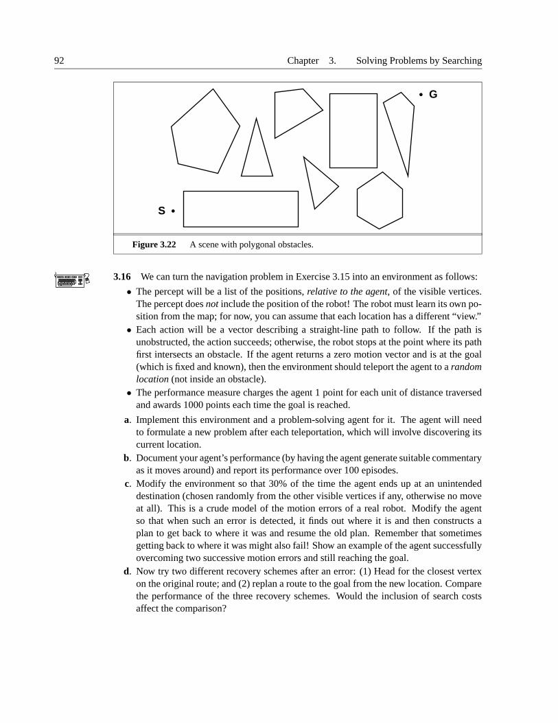
92 Chapter 3. Solving Problems by Searching
S
G
Figure 3.22 A scene with polygonal obstacles.
3.16 We can turn the navigation problem in Exercise 3.15 into an environment as follows:
• The percept will be a list of the positions, relative to the agent, of the visible vertices.The percept does not include the position of the robot! The robot must learn its own po-sition from the map; for now, you can assume that each location has a different “view.”• Each action will be a vector describing a straight-line path to follow. If the path is
unobstructed, the action succeeds; otherwise, the robot stops at the point where its pathfirst intersects an obstacle. If the agent returns a zero motion vector and is at the goal(which is fixed and known), then the environment should teleport the agent to a randomlocation (not inside an obstacle).• The performance measure charges the agent 1 point for each unit of distance traversed
and awards 1000 points each time the goal is reached.
a. Implement this environment and a problem-solving agent for it. The agent will needto formulate a new problem after each teleportation, which will involve discovering itscurrent location.
b. Document your agent’s performance (by having the agent generate suitable commentaryas it moves around) and report its performance over 100 episodes.
c. Modify the environment so that 30% of the time the agent ends up at an unintendeddestination (chosen randomly from the other visible vertices if any, otherwise no moveat all). This is a crude model of the motion errors of a real robot. Modify the agentso that when such an error is detected, it finds out where it is and then constructs aplan to get back to where it was and resume the old plan. Remember that sometimesgetting back to where it was might also fail! Show an example of the agent successfullyovercoming two successive motion errors and still reaching the goal.
d. Now try two different recovery schemes after an error: (1) Head for the closest vertexon the original route; and (2) replan a route to the goal from the new location. Comparethe performance of the three recovery schemes. Would the inclusion of search costsaffect the comparison?

Section 3.7. Summary 93
e. Now suppose that there are locations from which the view is identical. (For example,suppose the world is a grid with square obstacles.) What kind of problem does the agentnow face? What do solutions look like?
3.17 On page 62, we said that we would not consider problems with negative path costs. Inthis exercise, we explore this in more depth.
a. Suppose that actions can have arbitrarily large negative costs; explain why this possi-bility would force any optimal algorithm to explore the entire state space.
b. Does it help if we insist that step costs must be greater than or equal to some negativeconstant c? Consider both trees and graphs.
c. Suppose that there is a set of operators that form a loop, so that executing the set in someorder results in no net change to the state. If all of these operators have negative cost,what does this imply about the optimal behavior for an agent in such an environment?
d. One can easily imagine operators with high negative cost, even in domains such asroute finding. For example, some stretches of road might have such beautiful sceneryas to far outweigh the normal costs in terms of time and fuel. Explain, in precise terms,within the context of state-space search, why humans do not drive round scenic loopsindefinitely, and explain how to define the state space and operators for route finding sothat artificial agents can also avoid looping.
e. Can you think of a real domain in which step costs are such as to cause looping?
3.18 Consider the sensorless, two-location vacuum world under Murphy’s Law. Draw thebelief state space reachable from the initial belief state {1, 2, 3, 4, 5, 6, 7, 8}, and explain whythe problem is unsolvable. Show also that if the world is fully observable then there is asolution sequence for each possible initial state.
3.19 Consider the vacuum-world problem defined in Figure 2.2.
a. Which of the algorithms defined in this chapter would be appropriate for this problem?Should the algorithm check for repeated states?
b. Apply your chosen algorithm to compute an optimal sequence of actions for a 3× 3world whose initial state has dirt in the three top squares and the agent in the center.
c. Construct a search agent for the vacuum world, and evaluate its performance in a set of3× 3 worlds with probability 0.2 of dirt in each square. Include the search cost as wellas path cost in the performance measure, using a reasonable exchange rate.
d. Compare your best search agent with a simple randomized reflex agent that sucks ifthere is dirt and otherwise moves randomly.
e. Consider what would happen if the world were enlarged to n × n. How does the per-formance of the search agent and of the reflex agent vary with n?
Related Documents


