3. Descriptive Statistics 3. Descriptive Statistics • Describing data with tables and graphs Describing data with tables and graphs (quantitative or categorical variables) • Numerical descriptions of center, variability, position (quantitative variables) • Bivariate descriptions (In practice, most studies have several variables) studies have several variables)

Welcome message from author
This document is posted to help you gain knowledge. Please leave a comment to let me know what you think about it! Share it to your friends and learn new things together.
Transcript
3. Descriptive Statistics3. Descriptive Statistics
• Describing data with tables and graphsDescribing data with tables and graphs(quantitative or categorical variables)
• Numerical descriptions of center, variability, position (quantitative variables)
• Bivariate descriptions (In practice, most studies have several variables)studies have several variables)

1 Tables and Graphs
F di t ib ti Li t ibl l f
1. Tables and Graphs
Frequency distribution: Lists possible values of variable and number of times each occurs
Example: Student survey (n = 60) www stat ufl edu/ aa/social/data htmlwww.stat.ufl.edu/~aa/social/data.html
“ liti l id l ” d di l i bl“political ideology” measured as ordinal variable with 1 = very liberal, 4 = moderate, 7 = very conservativeconservative


Histogram: Bar graph of f ifrequencies or percentages

Shapes of histograms
• Bell-shaped (IQ, SAT, political ideology in all U.S. )Bell shaped (IQ, SAT, political ideology in all U.S. )• Skewed right (annual income, no. times arrested)• Skewed left (score on easy exam)Skewed left (score on easy exam)• Bimodal (polarized opinions)
Ex. GSS data on sex before marriage in Exercise 3.73: always wrong almost always wrong wrong onlyalways wrong, almost always wrong, wrong only sometimes, not wrong at all
category counts 238 79 157 409category counts 238, 79, 157, 409

Stem-and-leaf plotStem and leaf plotExample: Exam scores (n = 40 students)p ( )
Stem Leaf3 645 376 2358997 0113467789998 001112335688899 02238
2 Numerical descriptions2.Numerical descriptions
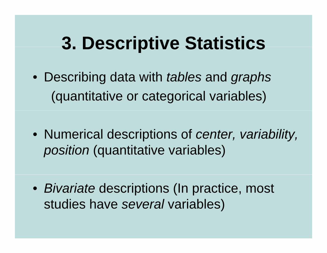
Let y denote a quantitative variable, withLet y denote a quantitative variable, with observations y1 , y2 , y3 , … , yn
a. Describing the center
Median: Middle measurement of ordered samplesa p e
Mean: 1 2 ... n iy y y yy + + + Σ= =Mean: y
n n= =
Example: Annual per capita carbon dioxide emissions (metric tons) for n = 8 largest nations in population size
Bangladesh 0.3, Brazil 1.8, China 2.3, India 1.2, Indonesia 1.4, Pakistan 0.7, Russia 9.9, U.S. 20.1
Ordered sample:
Median =
Mean = yy

Example: Annual per capita carbon dioxide emissions (metric tons) for n = 8 largest nations in population size
Bangladesh 0.3, Brazil 1.8, China 2.3, India 1.2, Indonesia 1.4, Pakistan 0.7, Russia 9.9, U.S. 20.1
Ordered sample: 0.3, 0.7, 1.2, 1.4, 1.8, 2.3, 9.9, 20.1
Median =
Mean = yy

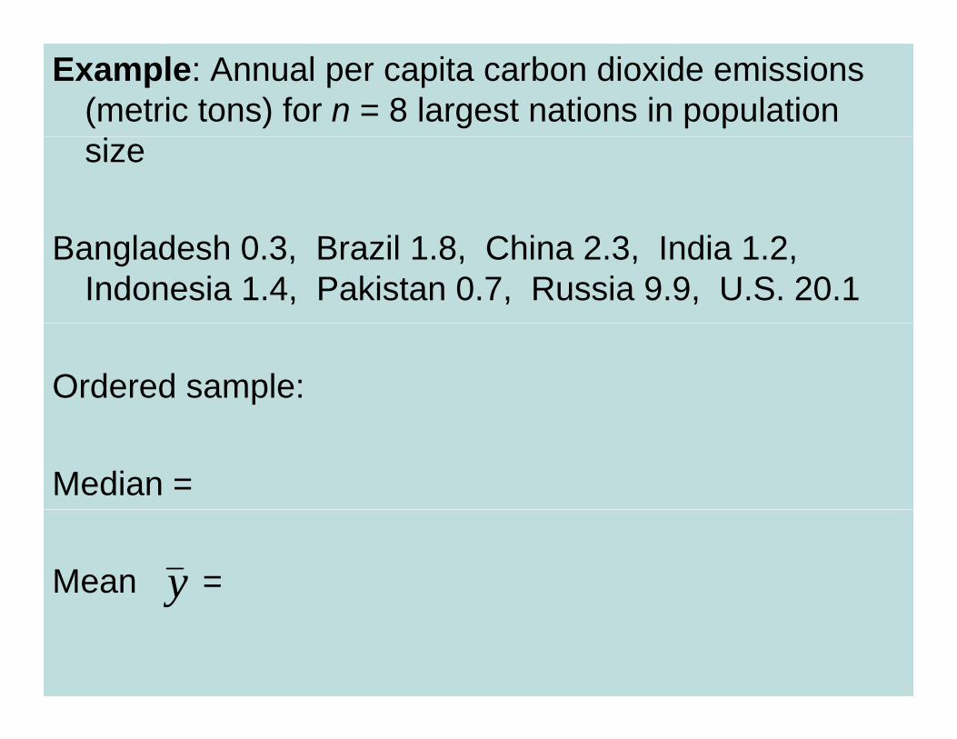
Example: Annual per capita carbon dioxide emissions (metric tons) for n = 8 largest nations in population size
Bangladesh 0.3, Brazil 1.8, China 2.3, India 1.2, Indonesia 1.4, Pakistan 0.7, Russia 9.9, U.S. 20.1
Ordered sample: 0.3, 0.7, 1.2, 1.4, 1.8, 2.3, 9.9, 20.1
Median = (1.4 + 1.8)/2 = 1.6
Mean = (0.3 + 0.7 + 1.2 + …+ 20.1)/8 = 4.7yy

Properties of mean and medianp
• For symmetric distributions, mean = mediany ,• For skewed distributions, mean is drawn in
direction of longer tail, relative to median• Mean valid for interval scales, median for
interval or ordinal scalesM iti t “ tli ” ( di ft• Mean sensitive to “outliers” (median often preferred for highly skewed distributions)
• When distribution symmetric or mildly skewed or• When distribution symmetric or mildly skewed or discrete with few values, mean preferred because uses numerical values of observations
Examples:
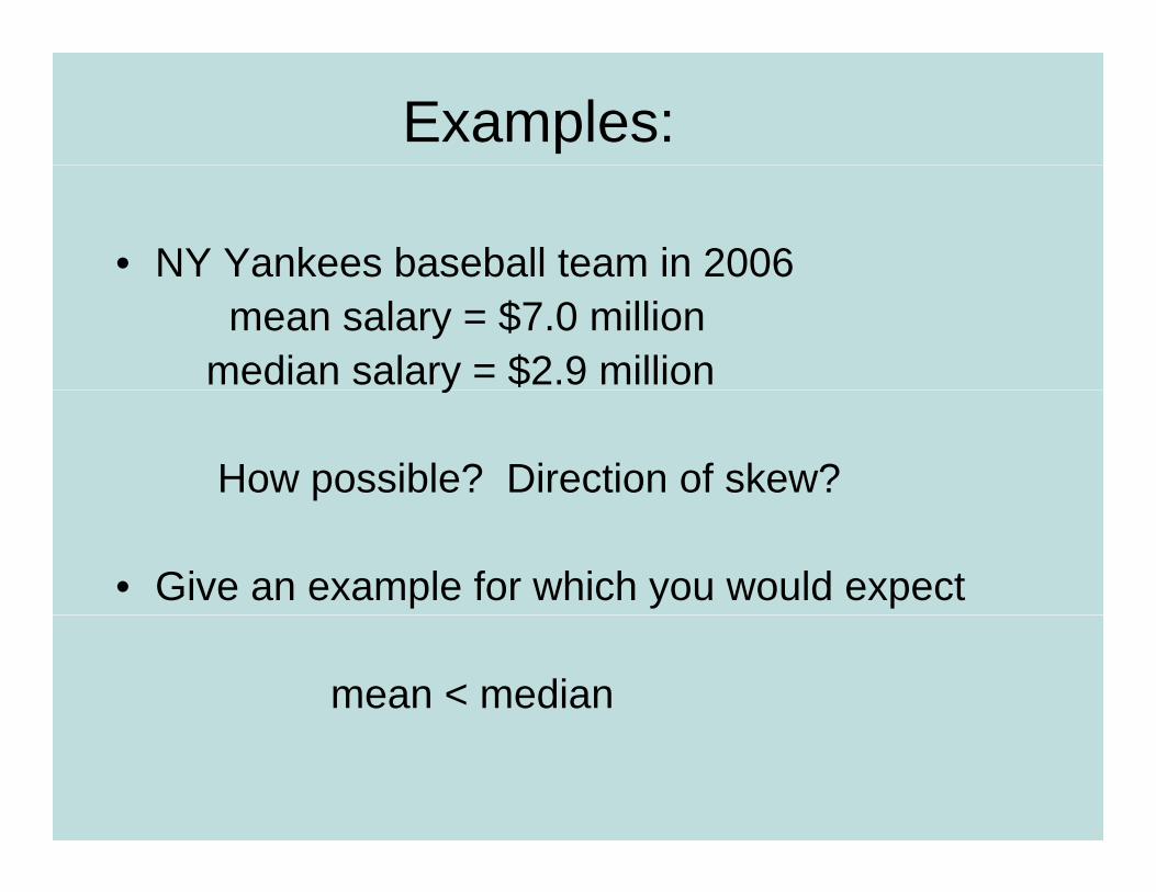
• NY Yankees baseball team in 2006 mean salary = $7.0 million
median salary = $2.9 milliony
How possible? Direction of skew?
• Give an example for which you would expect
mean < median
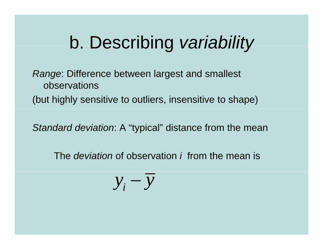
b Describing variabilityb. Describing variabilityRange: Difference between largest and smallest g g
observations(but highly sensitive to outliers, insensitive to shape)
Standard deviation: A “typical” distance from the mean
The deviation of observation i from the mean is
iy y−
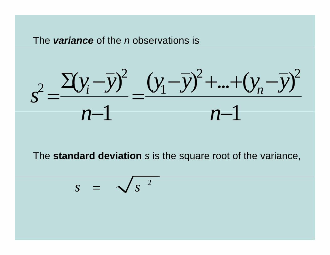
The variance of the n observations is
2 2 2( ) ( ) ( )y y y y y yΣ + +2 1( ) ( ) ... ( )1 1
i ny y y y y ysn n
Σ − − + + −= =
1 1n n− −
The standard deviation s is the square root of the variance,
2s s=
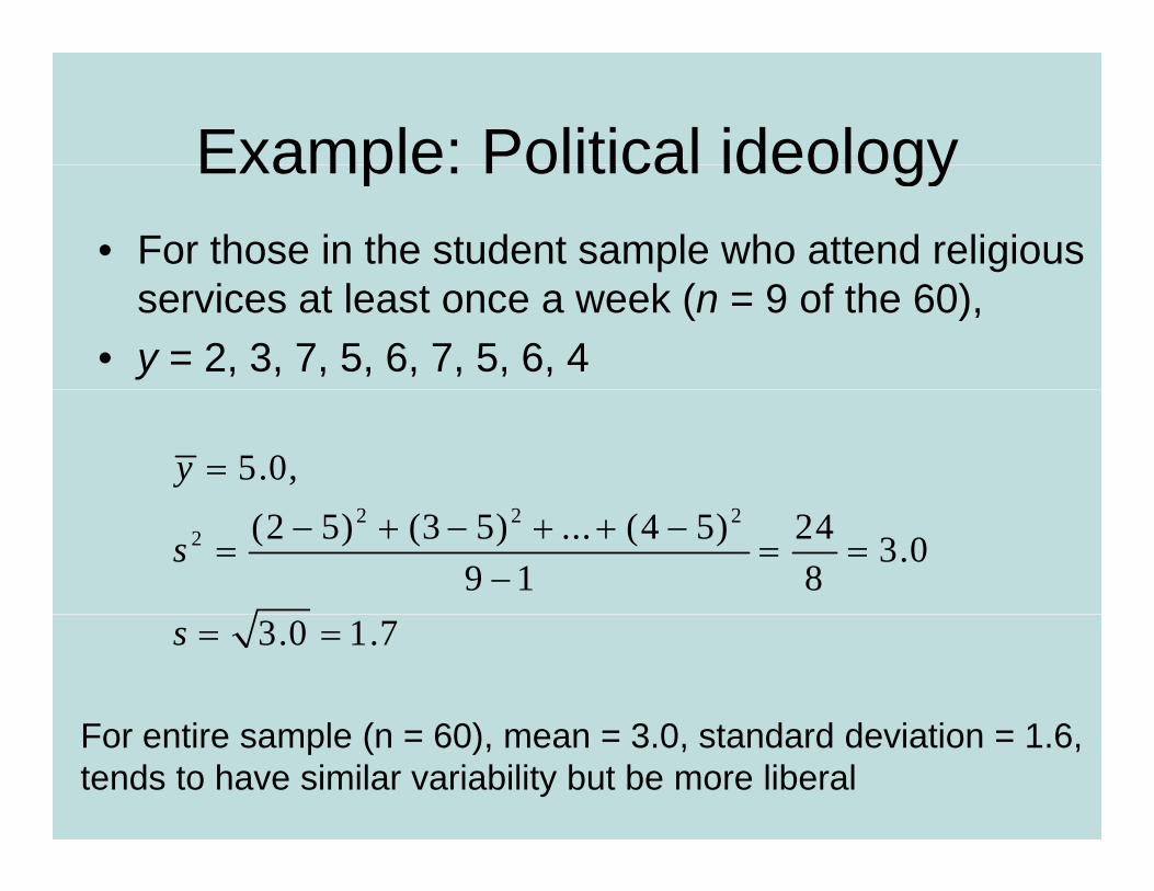
Example: Political ideologyExample: Political ideology• For those in the student sample who attend religious
services at least once a week (n = 9 of the 60), • y = 2, 3, 7, 5, 6, 7, 5, 6, 4
5.0,y =2 2 2
2 (2 5) (3 5) ... (4 5) 24 3.09 1 8
s − + − + + −= = =
−3.0 1.7s = =
F ti l ( 60) 3 0 t d d d i ti 1 6For entire sample (n = 60), mean = 3.0, standard deviation = 1.6, tends to have similar variability but be more liberal

• Properties of the standard deviation:
• s ≥ 0, and only equals 0 if all observations are equal
• s increases with the amount of variation around the means increases with the amount of variation around the mean
• Division by n - 1 (not n) is due to technical reasons (later)
• s depends on the units of the data (e g measure euro vs $)• s depends on the units of the data (e.g. measure euro vs $)
•Like mean, affected by outliers
•Empirical rule: If distribution approx. bell-shaped,
about 68% of data within 1 std. dev. of mean
b t 95% f d t ithi 2 td d fabout 95% of data within 2 std. dev. of mean
all or nearly all data within 3 std. dev. of mean

Example: SAT with mean = 500, s = 100(sketch picture summarizing data)(sketch picture summarizing data)
Example: y = number of close friends you haveExample: y number of close friends you haveRecent GSS data has mean 7, s = 11
Probably highly skewed: right or left?
Empirical rule fails; in fact, median = 5, mode=4
Example: y = selling price of home in Syracuse, NY. If mean = $130,000, which is realistic?
s=0, s=1000, s= 50,000, s = 1,000,000
c Measures of positionc. Measures of position
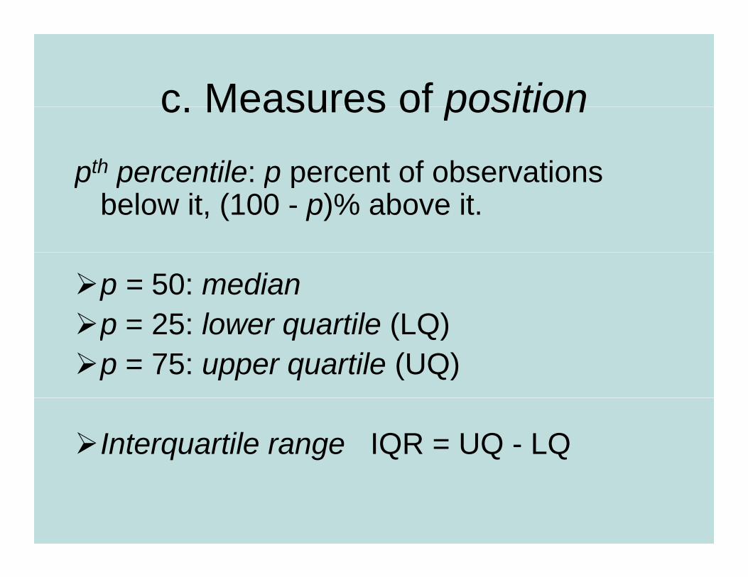
pth percentile: p percent of observationsp percentile: p percent of observations below it, (100 - p)% above it.
p = 50: medianp = 25: lower quartile (LQ)p = 25: lower quartile (LQ)p = 75: upper quartile (UQ)
Interquartile range IQR = UQ - LQ

Quartiles portrayed graphically by box plots (John T k 1977)Tukey 1977)Example: weekly TV watching for n=60 t d t 3 tlistudents, 3 outliers

Box plots have box from LQ to UQ, with median marked. They portray a five-y p ynumber summary of the data:
Minimum, LQ, Median, UQ, MaximumMinimum, LQ, Median, UQ, Maximumwith outliers identified separately
Outlier = observation fallingbelow LQ – 1.5(IQR)
or above UQ + 1.5(IQR)or above UQ 1.5(IQR)
E If LQ 2 UQ 10 th IQR 8 dEx. If LQ = 2, UQ = 10, then IQR = 8 and outliers above 10 + 1.5(8) = 22

Bivariate description
• Usually we want to study associations between two or more variables (e g how does number of closemore variables (e.g., how does number of close friends depend on gender, income, education, age, working status, rural/urban, religiosity…)
• Response variable: the outcome variable• Explanatory variable: defines groups to compare
Ex.: number of close friends is a response variable, while gender income are explanatory variableswhile gender, income, … are explanatory variables
Response = “dependent variable”Response = dependent variableExplanatory = “independent variable”

Summarizing associations:
• Categorical var’s: show data using contingency tables • Quantitative var’s: show data using scatterplots• Mixture of categorical var. and quantitative var. (e.g.,
number of close friends and gender) can give numerical summaries (mean, standard deviation) or side by side box plots for the groupsside-by-side box plots for the groups
E G l S i l S (GSS) d t• Ex. General Social Survey (GSS) dataMen: mean = 7.0, s = 8.4W 5 9 6 0Women: mean = 5.9, s = 6.0
Shape? Inference questions for later chapters?

Example: Income by highest degree

Contingency Tablesg y
• Cross classifications of categorical variables in which rows (typically) represent categories of explanatory variable and columns representexplanatory variable and columns represent categories of response variable.
• Numbers in “cells” of the table give the numbers of individuals at the corresponding combination ofindividuals at the corresponding combination of levels of the two variables
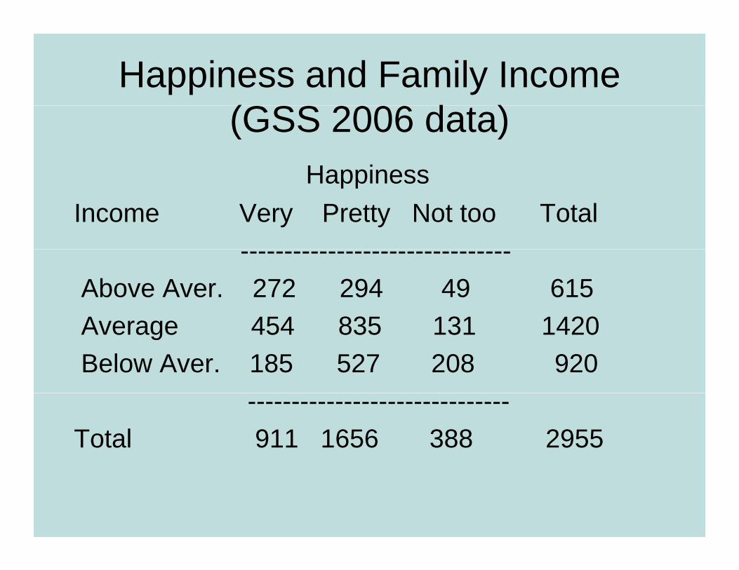
Happiness and Family Income (GSS 2006 d )(GSS 2006 data)
HappinessHappiness Income Very Pretty Not too Total
-------------------------------Above Aver. 272 294 49 615 Average 454 835 131 1420Average 454 835 131 1420 Below Aver. 185 527 208 920
------------------------------Total 911 1656 388 2955
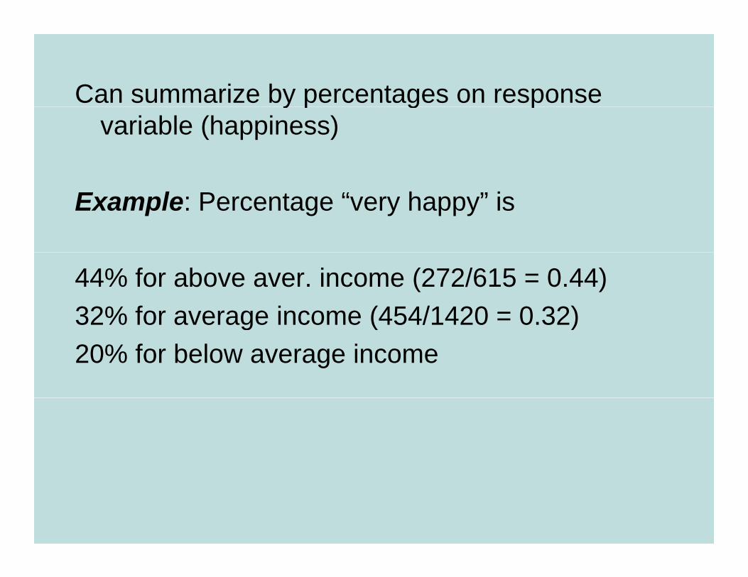
Can summarize by percentages on response y p g pvariable (happiness)
Example: Percentage “very happy” is
44% for above aver. income (272/615 = 0.44)32% for average income (454/1420 = 0.32)% g ( )20% for below average income

Happiness Income Very Pretty Not too Total
--------------------------------------------Above 272 (44%) 294 (48%) 49 (8%) 615 Average 454 (32%) 835 (59%) 131 (9%) 1420 Below 185 (20%) 527 (57%) 208 (23%) 920
----------------------------------------------
Inference questions for later chapters? (i.e., what can q p ( ,we conclude about the corresponding population?)

Scatterplots (for quantitative variables) plot i bl ti l i l tresponse variable on vertical axis, explanatory
variable on horizontal axis
Example: Table 9.13 (p. 294) shows UN data for several nations on many variables including fertility (births pernations on many variables, including fertility (births per woman), contraceptive use, literacy, female economic activity, per capita gross domestic product (GDP), cell-phone use, CO2 emissions
D t il bl tData available at http://www.stat.ufl.edu/~aa/social/data.html


Example: Survey in Alachua County, Florida, y yon predictors of mental health
(data for n = 40 on p. 327 of text and at ( pwww.stat.ufl.edu/~aa/social/data.html)
y = measure of mental impairment (incorporates various dimensions of psychiatric symptoms, including aspects of depression and anxiety)depression and anxiety)
(min = 17, max = 41, mean = 27, s = 5)
x = life events score (events range from severe personal disruptions such as death in family, extramarital affair, to l t h j b bi th f hild i )less severe events such as new job, birth of child, moving)
(min = 3, max = 97, mean = 44, s = 23)


Bivariate data from 2000 Presidential electionButterfly ballot Palm Beach County FL text p 290Butterfly ballot, Palm Beach County, FL, text p.290

Example: The Massachusetts Lottery(data for 37 communities, from Ken Stanley)
% income spent on lotterylottery
Per capita income

Correlation describes strength of i iassociation
Falls bet een 1 and +1 ith sign indicating direction• Falls between -1 and +1, with sign indicating direction of association (formula later in Chapter 9)
The larger the correlation in absolute value, the stronger the association (in terms of a straight line trend)the association (in terms of a straight line trend)
Examples: (positive or negative how strong?)Examples: (positive or negative, how strong?)Mental impairment and life events, correlation = GDP d f tilit l tiGDP and fertility, correlation = GDP and percent using Internet, correlation =

Correlation describes strength of associationassociation
Falls bet een 1 and +1 ith sign indicating direction• Falls between -1 and +1, with sign indicating direction of association
Examples: (positive or negative, how strong?)
Mental impairment and life events, correlation = 0.37GDP d f tilit l ti 0 56GDP and fertility, correlation = -0.56GDP and percent using Internet, correlation = 0.89


Regression analysis gives line di i ipredicting y using x
Example:Example: y = mental impairment, x = life events
Predicted y = 23.3 + 0.09x
e.g., at x = 0, predicted y = at x = 100 predicted y =at x = 100, predicted y =

Regression analysis gives line di i ipredicting y using x
Example:Example: y = mental impairment, x = life events
Predicted y = 23.3 + 0.09x
e.g., at x = 0, predicted y = 23.3at x = 100 predicted y = 23 3 + 0 09(100) = 32 3at x = 100, predicted y = 23.3 + 0.09(100) = 32.3
I f ti f l t h t ?Inference questions for later chapters?(i.e., what can we conclude about the population?)
Example: y = college GPA, x = high h l GPA f t d tschool GPA for student survey
What is the correlation?
What is the estimated regression equation?
We’ll see later in course the formulas that software uses to find the correlation and the “best fitting” regression equation

Sample statistics / Population parametersPopulation parameters
• We distinguish between summaries of samplesWe distinguish between summaries of samples(statistics) and summaries of populations(parameters).
• Common to denote statistics by Roman letters, parameters by Greek letters:p y
Population mean =μ, standard deviation = σ, proportion π are parameters.
In practice parameter values unknown we makeIn practice, parameter values unknown, we make inferences about their values using sample statistics.
• The sample mean estimates• The sample mean estimates the population mean μ (quantitative variable)
y
• The sample standard deviation s estimates the population standard deviation σ (quantitative variable)the population standard deviation σ (quantitative variable)
• A sample proportion p estimates p p p pa population proportion π (categorical variable)
Related Documents
![[PPT]I. Introduction - Department of Statisticsaa/sta6126/3. Descriptive statistics.ppt · Web viewTitle I. Introduction Author Administrator Last modified by agresti Created Date](https://static.cupdf.com/doc/110x72/5abe78157f8b9add5f8c8f2e/ppti-introduction-department-of-aasta61263-descriptive-statisticspptweb.jpg)