2nd ENTSO-E Guideline for Cost Benefit Analysis of Grid Development Projects 01 2nd ENTSO-E Guideline For Cost Benefit Analysis of Grid Development Projects FINAL – Approved by the European Commission 27 September 2018

Welcome message from author
This document is posted to help you gain knowledge. Please leave a comment to let me know what you think about it! Share it to your friends and learn new things together.
Transcript

2nd
EN
TSO
-E G
uide
line
for C
ost B
enefi
t Ana
lysi
s of
Gri
d D
evel
opm
ent P
roje
cts
01
2nd ENTSO-E Guideline For Cost Benefit Analysis of Grid Development Projects
FINAL – Approved by the European Commission 27 September 2018

2nd
EN
TSO
-E G
uide
line
for C
ost B
enefi
t Ana
lysi
s of
Gri
d D
evel
opm
ent P
roje
cts
02
1 INTRODUCTION AND SCOPE 6 1 Introduction and scope 8 1.1 Transmission system planning 9 1.2 Scope of the document 10 1.3 Content of the document 11
2 SCENARIO AND GRID DEVELOPMENT 12 2.1 Content of scenarios 14 2.2 Modelling framework 15 2.3 Baseline/reference network 16 2.4 Multi-case analysis 17 2.5 Optionally sensitivities 17
3 PROJECT ASSESSMENT: COMBINED COST-BENEFIT AND MULTI-CRITERIA ANALYSIS 18 3.1 Multi-criteria assessment 20 3.2 General assumptions 21 3.2.1 Clustering of investments 21 3.2.2 Transfer capability calculation 22 3.2.3 Geographical scope 24 3.2.4 Guidelines for Project NPV calculation 24 3.3 Assessment framework 25 3.4 Methodology for each benefit indicator 28 3.4.1 B1. Socio-economic welfare 28 3.4.2 B2. Variation in CO2 emissions 32 3.4.3 B3. RES integration 33 3.4.4 B4. Societal well-being as a result of RES integration and a change in CO2 emissions 34 3.4.5 B5. Variation in grid losses 34 3.4.6 B6. Security of supply: Adequacy to meet demand 36 3.4.7 B7. Security of supply: System flexibility 38 3.4.8 B8. Security of supply: System stability 40 3.5 Residual impact 41 3.5.1 S1. Residual environmental impact 41 3.5.2 S2. Residual social impact 41 3.5.3 S3. Other residual impacts 41 3.6 Costs 42 3.6.1 C1. CAPital EXpenditure (CAPEX) 42 3.6.2 C2. OPerating EXpenditure (OPEX) 42
4 ASSESSMENT OF STORAGE 44
5 ANNEXES 48 5.1 Annex 1: Technical criteria for planning 50 5.1.1 Definitions 50 5.1.2 Common criteria 51 5.2 Annex 2: Assessment of Internal Projects 53 5.3 Annex 3: Example of ΔNTC calculation 56 5.4 Annex 4: Impact on market power 58 5.5 Annex 5: Multi-criteria analysis and cost benefit analysis 59 5.6 Annex 6: Total surplus analysis 60 5.7 Annex 7: Value of lost load 64 5.8 Annex 8: Assessment of ancillary services 67 5.9 Annex 9: Residual environmental and social impact 68
Contents
2nd
EN
TSO
-E G
uide
line
for C
ost B
enefi
t Ana
lysi
s of
Gri
d D
evel
opm
ent P
roje
cts
1
Foreword
This document presents the second version of the ENTSO-E Guideline for Cost Benefit Analysis of Grid Development Projects (short: 2nd CBA guideline).
This new methodology is the result of “learning by implementing” and of taking into account stakeholder suggestions over a 3 years development process. During this period, it was also consulted with Member States and National Regulators and submitted to the official opinion of the Agency for Cooperation of Energy Regulators (ACER) and of the European Commission.
The Regulation (EC) 347/2013 mandates ENTSO-E to draft the European Cost Benefit Analysis methodology which shall be further used for the assessment of the Ten-Year Network Development portfolio. The first official CBA methodology drafted by ENTSO-E was approved and published by the European Commission on 5 February 2015.
This first edition of the CBA was used by ENTSO-E to assess projects in the 10-year network development plan (TYNDP) 2014 and 2016. ENTSO-E registered the impact of the TYNDP project assessment results on the European Commission Projects of Common Interest (EC PCI) process. This experience proved the need of a better methodology that allows a more consistent and comprehensive assessment of pan-European transmission and storage projects.
The 2nd CBA guideline has a more general approach than its predecessor and assumes that the project selection and definition, along with the scenarios description is within the frame of the TYNDP and therefore not defined in detail in the assessment methodology. ENTSO-E aims with this approach to develop a CBA methodology that can be used not only for one TYNDP but rather to include strong principles that would stand for a longer time. This new 2nd CBA guideline will be already used by ENTSO-E to assess projects benefits in the TYNDP 2018.
The present document includes after the CBA itself accompanying information on the compliance of the present CBA with the European Regulation, the changes that were made between the CBA 1 and 2, the way ENTSO-E responded to the official opinion of the European Commission and the roadmap for future evolutions of the CBA.
Why is the 2nd CBA guideline important?— This CBA guideline is the only European
methodology that consistently allows the assessment of TYNDP transmission and storage projects across Europe
— The outcomes of the CBA represent the main input in the European Commission Project of Common Interest (PCI) exercise
— The European CBA methodology is a source of learning for the national CBAs
2nd
EN
TSO
-E G
uide
line
for C
ost B
enefi
t Ana
lysi
s of
Gri
d D
evel
opm
ent P
roje
cts
1

2nd
EN
TSO
-E G
uide
line
for C
ost B
enefi
t Ana
lysi
s of
Gri
d D
evel
opm
ent P
roje
cts
2
General definitions
BoundaryA boundary represents a barrier to power exchanges in Europe, or in other words: a boundary represents a section (transmission corridor) within the grid where the capacity to transport the power flow related to the (targeted level of) power exchanges in Europe is insufficient.
In this context a boundary is referred to as a section through the grid in general. A boundary can:
a be the border between two bidding zones or countries;
b span multiple borders between multiple bidding zones or countries;
c be located inside a bidding zone or country dividing the area into two or multiple subareas.
Competing projects/investmentsTwo or more transmission projects are regarded as competing if they serve the same purpose, i.e. they are proposed to achieve a certain transmission capacity increase, but not all (proposed) projects are needed to achieve the necessary transmission capacity that serves this purpose. Usually, the competing transmission projects in such cases a) increase NTC on the same boundary; b) are in a similar stage of development; and c) would not be considered socio-economically viable if assessed under the assumption that the other project(s) is (are) also realized. These are not exclusive criteria, however.
Generation power shiftGeneration power shift is used to modify the market exchange across a specified boundary in order to find the maximum change in generation made possible by the grid. A generation power-shift can be seen as the deviation from the cost-optimal power plant dispatch (determined by market simulations) with the purpose to influence the grid utilisation1. For example, one can imagine the loading of a line across the boundary which separates System A from System B (with energy transported from A to B). Starting from this situation, generation can be incrementally increased in area A and decreased in area B. This process is carried out up to the point where the line loading security criteria in System A or System B is reached. The volume of the power shift represents the additional market exchange that is possible between these systems and should be reflected by the variation in NTC that is assumed in market simulations.
Grid Transfer Capability (GTC)The GTC is defined as the greatest (physical) power flow that can be transported across a boundary without the occurrence of grid congestions hereby taking into account the standard system security criterion as described in Annex 1.
InvestmentAn investment is defined as the smallest set of assets that together can be used to transmit electric power and that effectively add capacity to the transmission infrastructure. An example of an investment is a new circuit and the necessary terminal equipment and any associated transformers.
Investment needThe need to develop capacity across a boundary is referred to as an investment need. Since different scenarios may result in different power flows, the amount of capacity which is required to transport these power flows across a boundary and consequently the amount of investment needs, may differ from scenario to scenario.
Investment status— Investments are classified according to the
following statuses:— Under consideration: projects in the phase of
planning studies and consideration for inclusion in the national plan(s) and Regional / EU-wide Ten Year Network Development Plans (TYNDPs) of ENTSOs;
— Planned, but not yet in permitting: projects that have been included in the national development plan or completed the phase of initial studies (e.g. completed pre-feasibility or feasibility study), but have not initiated the permitting application yet;
— Permitting: starts from the date when the project promoters apply for the first permit regarding the implementation of the project and the application is valid;
— Under construction;— Commissioned (not relevant in the context
of clustering);— Cancelled (not relevant in the context of clustering).
1 This also can be seen as the definition of the redispatch. To avoid confusion in this case it is referred to generation power-shift as in reality the redispatch is of course used to reduce the grid utilization and to heal congestions. But as seen below in this guideline the redispatch will also be used to determine the theoretical maximum grid utilization by bringing the system to the edge of security.

2nd
EN
TSO
-E G
uide
line
for C
ost B
enefi
t Ana
lysi
s of
Gri
d D
evel
opm
ent P
roje
cts
3
Main investmentThe investment initially planned to achieve a certain goal, e.g. the interconnector between two bidding areas.
Net Transfer Capacity (NTC)The Net Transfer Capacity is a concept used in market models to represent the exchange capability between bidding zones. The NTC is defined by the maximum foreseen magnitudes of exchange programmes that can be operated between two bidding zones and should respect the system security conditions of the involved areas. As used for the application in the CBA the NTC has to be interpreted as a best estimated forecast to determine the ∆NTC for simulation purpose only.
Planning casesRepresentation of how the generation and transmission system could be managed one year along. The planning cases are point in time (snapshots) scenarios in order to represent in full detail the grid situations at these moments. Planning cases used in network studies are selected inter alia based on: a) the outputs from market studies, such as system dispatch, frequency and magnitude of constraints; b) regional considerations, such as wind and solar profiles or cold/heat spell; and c) results of pan-European Power Transfer Distribution Factor analysis (PTDF, when available).
ProjectA project is defined as a) a main investment that is built to fulfil a certain goal (e.g. to increase the capacity across a certain border by a certain amount), and b) one or more supporting investments that must be realised together with the main investment in order to make it possible for the main investment to realize its intended goal i.e. the full potential that is defined as the capacity increase of the main investment. In case there are no supporting investments needed, the project consists of just the main investment but will be nonetheless named ‘project’ in this guideline.
Put IN one at the Time (PINT) A methodology that considers each new investment/project (line, substation, phase shift transformer (PST) or other transmission network device) on the given network structure one-by-one and evaluates the load flows over the lines with and without the examined network investment/project reinforcement.
Reference networkThe network that includes all investments needed to reach the level of transfer capacity set as reference for a specific scenario and time horizon.
The reference network guides the application of the TOOT and PINT principles:— Investments within the reference network are
assessed via TOOT;— Investments on top of the reference network are
assessed in PINT.
ScenarioA set of assumptions for modelling purposes related to a possible future situation in which certain conditions regarding demand and installed generation capacity, infrastructures, fuel prices and global context occur.
Take Out One at the Time (TOOT)A methodology that consists of excluding projects from the forecasted network structure on a one-by-one basis in order to compare the system performance with and without the project under assessment.
Ten-Year Network Development Plan (TYNDP)The Union-wide report examining the development requirements for the next ten years carried out by ENTSO-E every other year as part of its regulatory obligation as defined under Article 8, paragraph 10 of Regulation (EU) 714/2009.
Time stepSimulation models compute their results at a given temporal level of detail. This temporal level of detail is referred to as the time step. Smaller time steps generally increase simulation run time, whereas larger time steps decrease simulation run time. Typically, simulations are done using one-hour time steps, but this level of granularity may vary depending on the required level of detail in the results.

2nd
EN
TSO
-E G
uide
line
for C
ost B
enefi
t Ana
lysi
s of
Gri
d D
evel
opm
ent P
roje
cts
4
Abbreviations
The following list shows abbreviations used in the 2nd ENTSO-E Guideline for Cost Benefit Analysis of Grid Development Projects:
Acronym Description
AC Alternating CurrentACER Agency for the Cooperation of Energy
RegulatorsCAPEX Capital Expenditure CostCBA Cost-Benefit-AnalysisCBCA Cross Border Cost AllocationCEER Council of European Energy
RegulatorsCIGRE Council on Large Electric SystemsDC Direct CurrentDSM Demand Side ManagementEC European CommissionEENS Expected Energy Not SuppliedENTSO-E European Network of Transmission
System Operators for ElectricityEPRI Electric Power Research InstituteETS Emissions Trading SchemeEU European UnionFCR Frequency Containment ReserveFRR Frequency Restoration ReserveGTC Grid Transfer CapabilityHHI Herfindahl Hirschman IndexHVDC High Voltage DCIEA International Energy AgencyITC Inter Transmission System Operator
Compensation for Transits
Acronym Description
KPI Key Performance IndicatorLOLE Loss of Load ExpectationMSC Mechanically Switched CapacitorsMSR Mechanically Switched ReactorsNPV Net Present ValueNTC Net Transfer CapacityOHL Overhead LineOPEX Operating Expenditure CostPCI Projects of Common InterestPINT Put IN one at the TimePTDF Power Transfer Distribution FactorRES Renewable Energy SourcesRR Replacement ReservesRSI Residual Supply IndexSEA Strategic Environmental AssessmentSEW Socio-Economic WelfareSMC Submarine CableSoS Security of SupplyTOOT Take Out One at the TimeTSO Transmission System OperatorTYNDP Ten-Year Network Development PlanUGC Underground CableVOLL Value of Lost LoadVSC Voltage Source Converter

2nd
EN
TSO
-E G
uide
line
for C
ost B
enefi
t Ana
lysi
s of
Gri
d D
evel
opm
ent P
roje
cts
5
2nd
EN
TSO
-E G
uide
line
for C
ost B
enefi
t Ana
lysi
s of
Gri
d D
evel
opm
ent P
roje
cts
5

6
Section 1
Introduction and scope
2nd
EN
TSO
-E G
uide
line
for C
ost B
enefi
t Ana
lysi
s of
Gri
d D
evel
opm
ent P
roje
cts
6

2nd
EN
TSO
-E G
uide
line
for C
ost B
enefi
t Ana
lysi
s of
Gri
d D
evel
opm
ent P
roje
cts
7
2nd
EN
TSO
-E G
uide
line
for C
ost B
enefi
t Ana
lysi
s of
Gri
d D
evel
opm
ent P
roje
cts
7

2nd
EN
TSO
-E G
uide
line
for C
ost B
enefi
t Ana
lysi
s of
Gri
d D
evel
opm
ent P
roje
cts
8
1
Introduction and scopeThis Guideline for Cost Benefit Analysis of Grid Development Projects is developed in compliance with the requirements of the EU Regulation (EU) 347/2013. The Regulation is intended to ensure a common framework for multi-criteria cost-benefit analysis (CBA) for TYNDP projects, which are the sole base for candidate projects of common interest (PCI). Moreover this guideline is recommended to be used as the standard guideline for project specific CBA as required by Regulation (EU) 347/2013 Article 12(a) for the CBCA process. In this regard all projects (including storage and transmission projects) and promoters (either TSO or third party) are treated and assessed in the same way.
The indicators are designed to support the specific requirements given in Article 4.2 of the Regulation in respect of market integration; sustainability (including the integration of renewable energy into the grid, energy storage, etc.) and security of supply. This is reflected in the structure of the main categories of the project assessment methodology described in the Guideline below.
The indicators defined in the Guideline are designed to be evaluated in compliance with the stipulations of the Regulation, as described in Annex IV.

2nd
EN
TSO
-E G
uide
line
for C
ost B
enefi
t Ana
lysi
s of
Gri
d D
evel
opm
ent P
roje
cts
9
1.1
Transmission system planningThe move to a more diverse power generation portfolio due to the rapid development of renewable energy sources (RES) and the liberalisation of the European electricity market has resulted in increasingly interdependent power flows across Europe, with large and correlated variations. Therefore, transmission system design must look beyond traditional (often national) Transmission System Operators’ (TSOs) boundaries and progress towards regional and European solutions. Close cooperation of ENTSO-E member companies, which are responsible for the future development of the European transmission system, is vital to achieve coherent and coordinated planning that is necessary for such solutions to materialise.
The main objective of transmission system planning is to ensure the development of an adequate pan-European transmission system which:— Enables safe grid operation;— Enables a high level of security of supply;— Contributes to a sustainable energy supply;— Facilitates grid access to all market participants;— Contributes to internal market integration, facilitates
competition, and harmonisation;— Contributes to energy efficiency of the system; and— Enables cross-country power exchanges.
In this process certain key rules have to be kept in mind, in particular:— Requirements and general regulations of the
liberalised European power and electricity market set by relevant EU legislation;
— EU policies and targets;— National legislation and regulatory framework;— Security of people and infrastructure;— Environmental policies and constraints;— Transparency in procedures applied; and— Economic efficiency.
The planning criteria to which transmission systems are designed are generally specified in transmission planning documents. Such criteria have been developed for application by individual TSOs taking into account the above mentioned factors, as well as specific conditions of the network to which they relate. Within the framework of the pan-European Ten Year Network Development Plan (TYNDP), ENTSO-E has developed common Guidelines for Grid Development (e.g. Annex 3 of TYNDP 2012). Thus, suitable methodologies have been adopted for future development projects and common assessments have been developed.
Furthermore, Regulation (EU) 347/2013 (hereafter referred to as: ‘the Regulation’) requests ENTSO-E to establish a “methodology, including on network and market modelling, for a harmonised energy system-wide cost-benefit analysis at Union-wide level for projects of common interest” (Article 11).
2nd
EN
TSO
-E G
uide
line
for C
ost B
enefi
t Ana
lysi
s of
Gri
d D
evel
opm
ent P
roje
cts
10
1.2
Scope of the documentThis document describes the common principles and procedures for performing combined multi-criteria and cost-benefit analysis using network, market and interlinked modelling methodologies (Chapter 2.2) for developing Regional Investment Plans and the Union-wide TYNDP, in accordance with Regulation (EU) 714/2009 of the 3rd Legislative Package. Following Regulation (EU) 347/2013 on guidelines for trans-European energy infrastructure, it also serves as a basis for a harmonised assessment of Projects of Common Interest (PCIs) at the European Union level.
When planning the future power system, new transmission assets are one of a number of possible system solutions. Other possible solutions include energy storage, generation, and demand-side management (DSM). Storage projects are therefore, in principle, assessed in a similar way as transmission projects even though their benefits sometimes lay more on the side of ancillary services, which are vital to the system, than on the classical CBA indicators. This is described in this CBA methodology in Chapter 4: Assessment of storage.
This CBA methodology sets out the ENTSO-E criteria for the assessment of costs and benefits of a transmission (or storage) project, all of which stem from European policies on market integration, security of supply and sustainability. In order to ensure a full assessment of all transmission benefits, some of the indicators are monetised, while others are quantified in their typical physical units (such as tonnes or GWh). A general overview of the indicators is given in Chapter 3.3, while a more detailed representation is given in Chapters 3.4, 3.5 and 3.6. This set of common indicators forms a complete and solid basis for project assessment across Europe, both within the scope of the TYNDP as well as for project portfolio development in the PCI selection process2.
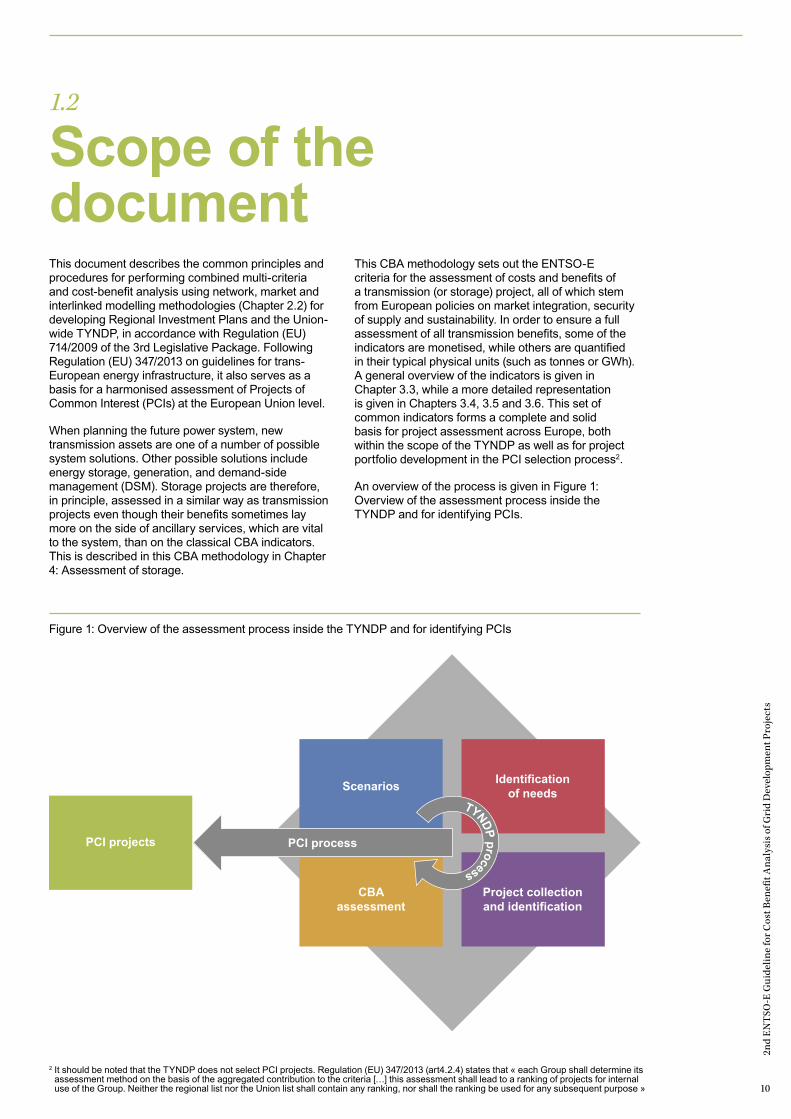
An overview of the process is given in Figure 1: Overview of the assessment process inside the TYNDP and for identifying PCIs.
Figure 1: Overview of the assessment process inside the TYNDP and for identifying PCIs
2 It should be noted that the TYNDP does not select PCI projects. Regulation (EU) 347/2013 (art4.2.4) states that « each Group shall determine its assessment method on the basis of the aggregated contribution to the criteria […] this assessment shall lead to a ranking of projects for internal use of the Group. Neither the regional list nor the Union list shall contain any ranking, nor shall the ranking be used for any subsequent purpose »
Scenarios
PCI projects
CBAassessment
Identification of needs
Project collection and identification
PCI process
TYNDP process

2nd
EN
TSO
-E G
uide
line
for C
ost B
enefi
t Ana
lysi
s of
Gri
d D
evel
opm
ent P
roje
cts
11
1.3
Content of the documentTransmission system development focuses on the long-term preparation and scheduling of reinforcements and extensions to the existing transmission grid. The identification of an investment need is followed by a project promoter(s) defining a project that addresses this need. Following Regulation (EU) 347/2013, these projects must be assessed under different planning scenarios, each of which represents a possible future development of the energy system. The aim of this document is to deliver a general guideline on how to assess these reinforcements from a cost and benefit point of view. Whilst their costs mostly depend on scenario independent factors like routeing, technology, material, etc., benefits strongly correlate with scenario specific assumptions. Therefore scenarios which define potential future developments of the energy system are used to gain an insight in the future benefits of transmission projects. The essence of scenario analysis is to come up with plausible pictures of the future. The assessment process takes place primarily in the context of TYNDP development according to the methodology that is described in this document. Although the scenarios are developed in the context of the biennial TYNDP cycle, a short overview of the scenario development process together with the modelling framework is provided in Chapter 2 of this CBA methodology.
A detailed description of the overall assessment, including the modelling assumptions and indicator structure, is given in Chapter 3.
The main assumptions and methodologies as used for transmission projects can also be applied for the assessment of storage. But, to also cover the unique properties of storage, a special guideline is given in Chapter 4.
The CBA methodology is developed to evaluate the benefits and costs of TYNDP projects from a pan-European perspective, providing important input for the selection process of PCIs. In this context the main objective of this CBA methodology is to provide a common and uniform basis for the assessment of projects with regard to their value for European society.
The cost-benefit impact assessment criteria adopted in this document reflect each project’s added value for society. Hence, economic and social viability are displayed in terms of increased capacity for trading of energy and balancing services between bidding areas (market integration), sustainability (RES integration, CO2 variation) and security of supply (secure system operation). The indicators also reflect the effects of the project in terms of costs and environmental viability. They are calculated through an iteration of market and network studies. It should be noted that some benefits are partly, or fully, internalised within other benefits such as avoided CO2 and RES integration via socio-economic welfare, while others remain completely non-monetised.
This is a continuously evolving process, so this document will be reviewed periodically, in line with prudent planning practice and further editions of the TYNDP, or upon request (as foreseen by Article 11 of the EU Regulation 347/2013).
12
Section 2
Scenario and grid development
Scenarios are constructed at the level of the European electricity system and can be adapted in more detail at a regional level. They reflect European and national legislation in force at the time of the analysis, and their effect on the development of these elements.
Scenarios are a description of plausible futures characterised by, amongst others, generation portfolio, demand forecast and exchange patterns with the systems outside the study region, etc. The scenarios are a representation of what the generation-transmission-consumption system could look like in the future and a means of addressing future
uncertainties and the interaction between these uncertainties. The objective is to construct contrasting future developments that differ enough from each other to capture a realistic range of possible futures that result in different challenges for the grid. These different future developments can be used as input parameter sets for subsequent simulations.
Scenarios are the basis for the further calculation of the grid development needs. All projects included in the TYNDP must be assessed against the same set of scenarios (provided that the project is assessed for a given reference year). 2
nd E
NT
SO-E
Gui
delin
e fo
r Cos
t Ben
efit A
naly
sis
of G
rid
Dev
elop
men
t Pro
ject
s
12

2nd
EN
TSO
-E G
uide
line
for C
ost B
enefi
t Ana
lysi
s of
Gri
d D
evel
opm
ent P
roje
cts
13
2nd
EN
TSO
-E G
uide
line
for C
ost B
enefi
t Ana
lysi
s of
Gri
d D
evel
opm
ent P
roje
cts
13
2nd
EN
TSO
-E G
uide
line
for C
ost B
enefi
t Ana
lysi
s of
Gri
d D
evel
opm
ent P
roje
cts
14
2.1
Content of scenariosMulti-criteria, cost-benefit analysis of candidate projects of European interest are based on the scenarios developed in ENTSO-E’s TYNDP. These visions provide the framework within which the future is likely to occur, but does not attach a probability of occurrence to them. Some TYNDP visions have a stronger national focus than others; some are ‘top-down’; others are ‘bottom-up’ etc. There is no right or wrong; likely or unlikely option: all visions have to be treated equally and, due to the uncertainties of the future energy sector, no scenario can be defined as a ‘leading scenario’. These scenarios aim to provide stakeholders in the European electricity market with an overview of generation, demand and their adequacy in different scenarios for the future ENTSO-E power system, with a focus on the power balance, margins, energy indicators and generation mix. The scenarios are elaborated after formally consulting Member States and the organisations representing all relevant stakeholders.
Scenarios can be distinguished depending on the time horizon (see also Figure 4):
— Mid-term horizon (typically 5 to 10 years): Mid-term analyses should be based on a forecast for this time horizon. ENTSO-E’s Regional Groups and project promoters will have to consider whether a new analysis has to be made or analysis from last TYNDP (i.e. former long term analysis) can be re-used;
— Long-term horizon (typically 10 to 20 years): Long-term analyses will be systematically assessed and should be based on common ENTSO-E scenarios;
— Very long-term horizon (typically 20 to 40 years): Analysis or qualitative considerations could be based on the ENTSO-E 2050-reports;
— Horizons which are not covered by separate data sets will be described through interpolation techniques.
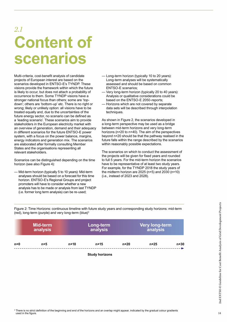
As shown in Figure 2, the scenarios developed in a long-term perspective may be used as a bridge between mid-term horizons and very long-term horizons (n+20 to n+40). The aim of the perspectives beyond n+20 should be that the pathway realised in the future falls within the range described by the scenarios within reasonably possible expectations.
The scenarios on which to conduct the assessment of the projects will be given for fixed years and rounded to full 5 years. For the mid-term horizon the scenarios have to be representative of at least two study years. For example, for the TYNDP 2018 the study years of the midterm horizon are 2025 (n+5) and 2030 (n+10) (i.e., instead of 2023 and 2028).
Figure 2: Time Horizons: continuous timeline with future study years and corresponding study horizons: mid-term (red), long-term (purple) and very long-term (blue)3
3 There is no strict definition of the beginning and end of the horizons and an overlap might appear, indicated by the gradual colour gradients used in the figure.
Mid-term analysis
n+0 n+5 n+10 n+15 n+20 n+25 n+30
Study horizons
Long-term analysis
Very long-term analysis

2nd
EN
TSO
-E G
uide
line
for C
ost B
enefi
t Ana
lysi
s of
Gri
d D
evel
opm
ent P
roje
cts
15
2.2
Modelling frameworkMarket simulationsMarket studies are used to calculate the cost optimal dispatch of generation units under the constraint that the demand for electricity is fulfilled in each bidding area and in every modelled time step4. Besides the dispatch of generation and demand (if modelled endogenously), market simulations compute the market exchanges between bidding areas and corresponding marginal costs for every time step. Market studies are used to determine the benefits of providing additional transport capacity and enabling a more efficient usage of generation units available in different locations across bidding areas. They take into account several constraints such as flexibility and availability of thermal units, hydro conditions, wind and solar profiles, load profile and outages. They also allow the measurement of savings in generation costs due to the investments in the grid (and/or in storage).
Market studies results allow the computation of some of the CBA indicators, such as socio-economic welfare (SEW), CO2 emissions, RES integration and the adequacy component of security of supply. The output of market simulations will be used as an input for defining the generation, consumption and power flows in the grid, allowing load flow calculations to be performed.
There are different options to represent the transmission network in market models, namely:— NTC-based market simulations
Using a simplified (NTC) model of the physical grid, the bidding areas are represented as a network of interconnected nodes connected by a transport capacity that is available for market exchanges (NTC). These NTC values represent an approximation of the potential for market exchanges using the physical (direct or indirect5) interconnections that exist between each pair of bidding areas. Thus, the market studies analyse the cost-optimal generation pattern for every time step under the assumption of perfect competition.
— Flow-based simulations Flow-based market simulations combine market and network studies, which consider the interrelation between the power-flow as obtained from network simulations and the corresponding potential for market exchanges, and vice versa. Flow-based market simulations take into account the relationships between each potential market
exchange and its corresponding utilization of the physical grid capacities (cross-border as well as internal grid). Flow-based market simulations thus use (a representation of) the physical grid capacities to define the constraints for market exchanges rather than a set of independent NTC values.
Network simulationsNetwork studies represent the transmission network in a high level of detail and are used to calculate the actual load flows that take place in the network under given generation/load/market exchange conditions (also see Annex 1). Network studies allow bottlenecks in the grid corresponding to the power flows resulting from the market exchanges to be identified.
Network studies results allow the computation of some of the CBA indicators such as: NTC, grid losses and the stability component of the security of supply.
Both types of studies – market and network – thus provide different information. They generally complement one another and are therefore often used in an iterative manner.
Re-dispatch simulationsFor internal projects (defined as projects which are related to developing capacities across boundaries within bidding areas rather than across bidding areas), a combination of both network and market studies can be applied to combine network contingencies with the economy of the generation dispatch (see Annex 2). These re-dispatch simulations compute the cost of alleviating overloads (taken from network simulations) by adjusting the initial dispatch (taken from market simulations) while maintaining the same power plant specific constraints that were also applied for the market simulations such as minimum up- and down times, ramp rates, must-run obligations, variable costs, etc.
Re-dispatch simulations assist in the computation of the CBA indicators (the same as for market simulations) when it concerns the evaluation of internal projects using the initial generation dispatch from NTC-based market simulations as a starting point.
Flow-based market simulations can offer an alternative approach to compute the CBA indicators for internal projects.
4 Typically market simulations apply a one-hour time step, which is in accordance with the time step used in most electricity wholesale markets. This CBA Methodology is independent from the chosen time step, however.
5 In general the market flow is different from the corresponding physical flow as for getting the trading capacities e.g. ring flows are not needed to be considered. The important information is the trading capacity between two markets.

2nd
EN
TSO
-E G
uide
line
for C
ost B
enefi
t Ana
lysi
s of
Gri
d D
evel
opm
ent P
roje
cts
16
2.3
Baseline/reference networkProject benefits are calculated as the difference between a simulation which does include the project and a simulation which does not include the project. The two proposed methods for project assessment are as follows:— Take Out One at the Time (TOOT) method, where
the reference case reflects a future target grid situation in which all additional network capacity is presumed to be realised (compared to the starting situation) and projects under assessment are removed from the forecasted network structure (one at a time) to evaluate the changes to the load flow and other indicators.
— Put IN one at the Time (PINT) method, where the reference case reflects an initial state of the grid without the projects under assessment, and projects under assessment are added to this reference case (one at a time) to evaluate the changes to the load flow and other indicators.
As the selection of the reference case has a significant impact on the outcome of an individual project assessment, a clear explanation of it must be given. This should include an explanation of the initial state of the grid, in which none of the projects under assessment in the relevant study is included. The reference network is then built up of including the most mature projects that are: a) in the construction phase or b) in the ‘permitting’ or ‘planned but not yet permitting’ phase where their timely realisation is most likely e.g. when the country specific legal requirements have stated the need of the projects to being realised.
Projects in the ‘under consideration’ phase are seen as non-mature and have therefore generally to be excluded from the reference grid leading to an assessment using the PINT approach.
To obtain the NTC value of the reference network the NTC increases of each single (non-competing) project has to be taken into account. As different scenarios with different assumptions might have different expected capacities, this also has to be reflected by the reference network, i.e. it has to be clearly explained that the reference network reflects the assumptions made by the scenarios.
The TOOT and PINT methods are to be applied consistently for both market and network simulations. For the latter method, the reference network is clearly defined by the network model that is used; and for market simulations the reference network takes into account the exchange capacities between the defined market zones including the additional capacity brought by the projects included in the grid (e.g. when using the TOOT approach, each project under assessment has to be added to the grid model and its contribution to commercial capacity has to be added to the respective boundaries).
The TOOT method provides an estimation of benefits for each project, as if it were the last to be commissioned. In fact, the TOOT method evaluates each new development project into the whole forecasted network. The advantage of this analysis is that it immediately appreciates every benefit brought by each project, without considering the order of projects. All benefits are considered in a conservative manner, in fact each evaluated project is considered into an already developed environment, in which all programmed development projects are present. Hence, this method allows analyses and assessments at TYNDP level, considering the whole future system environment and every future network evolution.
In general, application of the TOOT approach underestimates the benefits of projects because all project benefits are calculated under the assumption that the project is the last (marginal) project to be realised. Project benefits are generally negatively affected by the presence of other projects (i.e. if one project gets built, a second will have lower benefits). This effect is generally the strongest when two (or more) projects are constructed to achieve a common goal across the same boundary, although it may also be present when projects are constructed along different boundaries.
For interdependent projects, the strict application of TOOT may not fully reflect the benefits of the projects. Therefore in addition to the project benefits as calculated under the strict application of TOOT, the benefits can be calculated in relation to the realisation of other projects on the same boundary (multiple TOOT) and additionally present these results in the TYNDP. When the multiple TOOT method is applied a detailed description of the sequence of projects must be given.
Figure 3: Illustration of TOOT and PINT approaches
B
C
D
B
C
D
B
C
DA
Reference grid Take one OUT at a Time (TOOT)
Put one IN at a Time (PINT)Approach
A
A

2nd
EN
TSO
-E G
uide
line
for C
ost B
enefi
t Ana
lysi
s of
Gri
d D
evel
opm
ent P
roje
cts
17
2.4
Multi-case analysis
2.5
Optionally sensitivities
System planning studies are carried out with market simulations producing results for each time step (typically one hour). The network studies then perform load flow calculations using these results for each time step. In order to reduce the number of required network calculations, network studies may group results from several time steps into one planning case. The results for each planning case are then considered as representative for all the time steps that are linked to it. It is crucial that the choice of planning cases and
the time steps that they represent are adequate, i.e. that the planning cases selected out of the available cases for each time step are representative of the year-round effect of the generation dispatch, load dispatch and market exchanges within the area under consideration. The process of obtaining a representative set of planning cases depends greatly on the (combination of) dispatch, load, and exchange profiles, and especially on the availability profiles for variable renewable energy sources.
Sensitivity analysis can be performed with the intention of observing how certain changes of scenario (e.g. by changing only one parameter or a set of interlinked parameters) affects the model results in order to achieve a deeper understanding of the system’s behaviour regarding these parameters. In principle, each individual model parameter can be used for a sensitivity analysis, but not all might be equally useful to obtain the desired information. Furthermore, different parameters can have a different impact on the results, depending on the scenario and it is therefore recommended to perform detailed scenario-specific studies to determine the most impacting parameters. Based on the experience of previous TYNDPs the parameters listed below could be optionally be used to perform sensitivity studies. This list is not exhaustive and provides some examples of useful sensitivities.
— Fuel and CO2-Price Within the scenario development process a global set of values for fuel prices is defined. Nevertheless a certain degree of uncertainty for 2030 is unavoidable. Fuel and CO2-prices determine the specific costs of conventional power plants and thus the merit order. Therefore varying fuel and CO2-prices to see the impact of merit order shifts to CBA-results is a valuable sensitivity.
— Climate year Using historic climate data of different years might influence the benefits of a project. For example the indicator RES-integration depends on the infeed
of RES and thus on weather conditions. For this reason performing analysis with different climate years would lead to a deeper understanding of how market results depend on weather conditions.
— Load Regarding the development of load, two opposed drivers can be identified. On the one hand energy efficiency will lead to decreasing load; and on the other hand, more and more applications will be electrified (e.g. e-mobility, heat pumps etc.), which will lead to an increasing load. Sensitivity analysis of load could be conducted by varying the peak load and/or the annual energy that is needed.
— Technology phase-out Due to external circumstances, a phase-out of a specific technology (e.g. Nuclear or Lignite) could occur and lead to a transition of the whole energy system within a member state. Such developments cannot be foreseen and are not considered within the scenario framework.
— Must-run If thermal power plants provide not only electrical power but also heat, then thermal power “must-run” boundary conditions are used in market simulations, i.e. these power plants cannot be shut down and have to operate in specific time frames and at least at a minimum level in order to ensure heat production. By assuming different must-run conditions for conventional power plants, market results will differ.

18
Section 3
Project assessment: combined cost-benefit and multi-criteria analysis
The goal of project assessment is to characterise the impact of transmission projects, both in terms of added value for society (increase of capacity for trading of energy and balancing services between bidding areas, RES integration, increased security of supply), as well as in terms of costs.
The goal of project assessment is to characterise the impact of transmission projects, both in terms of added value for society (increase of capacity for trading of energy and balancing services between bidding areas, RES integration, increased security of supply), as well as in terms of costs.
It is the task of ENTSO-E to define a robust and consistent methodology to assess the contribution of projects across Europe on a consistent basis. ENTSO-E developed this CBA methodology to achieve a uniform assessment process for transmission projects across Europe.
A robust assessment of transmission projects, especially in a meshed system, is a complex matter. Additional transmission infrastructure provides more transmission capacity and hence allows for an optimization of the generation portfolio, which leads to an increase of Socio-Economic Welfare (SEW)
throughout Europe. Further benefits such as Security of Supply (SoS) or improvements of the flexibility also have to be taken into due account.
The assessment of costs and benefits are undertaken using combined cost-benefit and multi-criteria approach within which both qualitative assessments and quantified, monetised assessments are included. In such a way the full range of costs and benefits can be represented, highlighting the characteristics of a project and providing sufficient information to decision makers.
Such an approach recognises that a fully monetized approach is not practically feasible in this context as many benefits cannot be economically quantified in an objective manner. Examples of such benefits include system safety and environmental impact. Multi-criteria analysis however can account for each of these including the compilation of a cost-benefit analysis of those elements that can be monetized, while recognising that other elements also exist that are not quantified.
This chapter establishes a methodology for the clustering of investments into projects6; defines each of the cost and benefit indicators; and the project assessment required for each indicator.
6 In general a project can also consist of only one investment. Obviously in this case no clustering rule has to be applied.
2nd
EN
TSO
-E G
uide
line
for C
ost B
enefi
t Ana
lysi
s of
Gri
d D
evel
opm
ent P
roje
cts
18

2nd
EN
TSO
-E G
uide
line
for C
ost B
enefi
t Ana
lysi
s of
Gri
d D
evel
opm
ent P
roje
cts
19
2nd
EN
TSO
-E G
uide
line
for C
ost B
enefi
t Ana
lysi
s of
Gri
d D
evel
opm
ent P
roje
cts
19

2nd
EN
TSO
-E G
uide
line
for C
ost B
enefi
t Ana
lysi
s of
Gri
d D
evel
opm
ent P
roje
cts
20
3.1
Multi-criteria assessmentThe overall assessment is displayed as a combined cost-benefit and multi-criteria matrix in the TYNDP, as shown in Section 3.4. All indicators are quantified. Costs, socio-economic welfare and the variation of transmission losses are displayed in Euros. The other indicators are displayed using the most relevant units ensuring both a coherent measure across Europe and an opposable value, while avoiding the double accounting in Euros. Indeed, some benefits like avoided CO2 and RES integration are already internalised in socio-economic welfare but are also displayed as they are part of the EU 20-20-20 targets.
Using this combined cost-benefit and multi-criteria assessment each project is characterised by its impact of both the added value for society and in terms of costs in a standardised way. Therefore the overall impacts, positive as well as negative, for each project can be compared. The overall combined cost-benefit
and multi-criteria assessment of transmission projects, especially in a meshed system, is a complex matter and highlights the characteristics of a project and gives sufficient information to the decision-makers. Only by considering all of the indicators can the total benefit of a project be described, while the importance of each indicator might be project specific: the main aim of one project might be to significantly integrate large amounts of RES into the grid, while for another the focus may lies more on increasing the security of supply by means of connecting highly flexible generation units. In both cases the monetised benefits (determined by the monetised indicators) may be the key driving indictors for making an investment decision, but they may not the only ones.
The following figure displays a simplified overview of the whole process of project assessment resulting in the set of CBA indicators.
Figure 4: Schematic project assessment process. While “CBA market” and “CBA network indicators” are the direct outcome of market and network studies, respectively, “project costs” and “residual impacts” are obtained without the use of simulations.
Project assessment
Project costsProject definition and
technical capacity
Market simulation
Scenario
Grid modelNetwork
simulation
CBA market indicators
Residual impact indicators
Generation, consumption and exchange patterns
CBA network indicators
2nd
EN
TSO
-E G
uide
line
for C
ost B
enefi
t Ana
lysi
s of
Gri
d D
evel
opm
ent P
roje
cts
21
3.2
General assumptions
3.2.1 Clustering of investments
This sub-section provides the general guidance necessary to assess projects beyond the calculation of the individual indicators. It provides guidelines for clustering; computation of transfer capability (i.e. in meshed networks the physical capacity of the
investment is usually different from is capability to accommodate a market transfer); the geographic scope to take into consideration; and, the calculation of a net-present value on the basis of the (monetized) indicators that are available for the project.
In some cases it may be necessary to realize a group of investments together in order to develop transmission capacity (i.e. one investment cannot perform its intended function without the realisation of another investment). This process is referred to as the clustering of investments. Project assessment is done for the combined set of clustered investments.
When investments are clustered, it must be clearly demonstrated why this is necessary. Investments should only be clustered together if an investment contributes to the realization of the full potential of another (main) investment. Investments which contribute only marginally to the full potential of the main investment are not allowed to be clustered together.
The full potential of the main investment represents its maximum transmission capacity in normal operation conditions. When clustering investments, one must explicitly define a main investment (e.g., an interconnector), which is supported by one or more supporting investments. A project that consists of more than one investment is thus defined as a main
investment with one or more supporting investments attached to it.
Note that competing investments cannot be clustered together. Further limitations are as follows:— If an investment is significantly delayed7 compared
to the previous TYNDP, it can no longer be clustered within this project. In order to avoid that investments are clustered when they are commissioned far apart in time (which would also introduce a risk that one or more investments in the project are never realized eventually), a limiting criterion is introduced that prohibits clustering of investments that are more than one status away.
— Investments can only be clustered if they are at maximum one stage of maturity apart from each other. This limiting criterion is introduced in order to avoid excessive clustering of investments that do not contribute to realizing the same function because they are commissioned too far ahead in time.
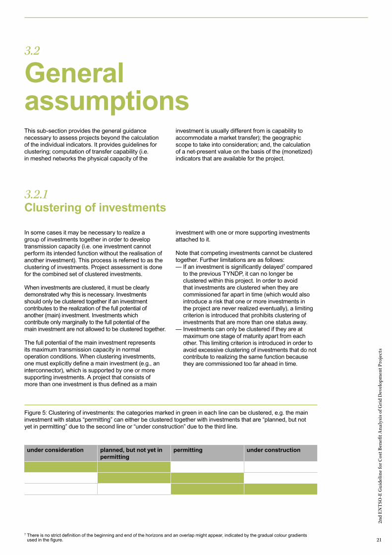
Figure 5: Clustering of investments: the categories marked in green in each line can be clustered, e.g. the main investment with status “permitting” can either be clustered together with investments that are “planned, but not yet in permitting” due to the second line or “under construction” due to the third line.
under consideration planned, but not yet in permitting
permitting under construction
7 There is no strict definition of the beginning and end of the horizons and an overlap might appear, indicated by the gradual colour gradients used in the figure.

2nd
EN
TSO
-E G
uide
line
for C
ost B
enefi
t Ana
lysi
s of
Gri
d D
evel
opm
ent P
roje
cts
22
3.2.2 Transfer capability calculation
There are two notions of transfer capability that this Methodology refers to: Net Transfer Capacity, which is related to the potential for market exchanges of electricity resulting in a power shift of dispatch from one bidding zone to another; and, Grid Transfer Capacity, which is related to physical power flows that can be accommodated by the grid.
The Net Transfer Capacity (NTC) reflects the ability of the grid to accommodate a market exchange between two neighbouring bidding areas. An increase in NTC (ΔNTC) can be interpreted as an increased ability for the market to commercially exchange power, i.e. to shift power generation from one area to another area (or similarly for load). The physical power flow that is the result of this power shift may or may not directly flow across the border of the two neighbouring bidding areas in its entirety, but may or may not transit through third countries. The increase of the ability to accommodate market exchanges as a result of increasing physical transmission capacity may therefore be different from the capability of the grid to transport physical power across the border.
Since the exchanges between bidding zones result in power flows making use of the transport capacity across the different boundaries they impact, an increase in GTC across a specific boundary is “ceteris paribus” illustrative of the increased exchange capability between these bidding zones. The “ceteris paribus” statement acknowledges that, in actual system operations, one single boundary is not exclusively influenced by only the exchanges between the bidding zones it relates to. The physical flow on the boundary can also be influenced by exchanges between other bidding zones which, for example, cause loop or transit flows. These influences are not taken into account when calculating the increased NTC delivered by a project in the context of this methodology.
Note that while the concept of NTC calculations in the context of long-term studies is similar to the operational calculation of NTC values on borders, the concept of NTC as defined for the purpose of long-term planning studies may show some differences in the sense that the approaches may not consider the same operational considerations to ensure a safe and reliable operation of the system. The NTC values reported in long-term studies are calculated under the “ceteris paribus” assumption that nothing else in the system changes
(e.g. generation and load in neighbouring zones; RES fluctuations; loop flows) and therefore does not have an impact on the calculated power shift made possible by the project (i.e. which equals market exchange). In the TYNDP, the assumed utilisation of the additional grid transfer capability delivered by a project will be reported in terms of ability for additional commercial exchanges (i.e. ΔNTC) between the bidding zones that define the boundary in question. Note that the ΔNTC is directional, which means that values might be different in either direction of the commercial power flow across a boundary.
ΔNTC is calculated using network models by applying a generation power shift8 across the boundary under consideration. This figure applies to the year-round situation (i.e. 8,760 hours) of how the generation power shift affects the power flow across the boundary under analysis. Calculating a ΔNTC value generally results in a different value for each simulated time step of the year under consideration. This year-round situation should be reflected in the load flow analysis either via a simulation of each individual time step, or via a simulation of a set of points in time which are representative of the year-round situation. The weighted average ΔNTC per time step is then reported.
The calculation of the ΔNTC is based upon a reference network model in line with the scenario considered. As ΔNTC is the result of the possible power shift, the figure may differ between scenarios. If the differences between scenarios are significant, project promoters must report a range of values.
A detailed example on how the ΔNTC can be calculated is given in Annex 3.
The Grid Transfer Capability (GTC) reflects the ability of the grid to transport physical electricity across a boundary in compliance with relevant operational standards for safe system operation. A boundary usually represents a bottleneck in the power system where the transfer capability is insufficient to accommodate the power flows (resulting from the dispatch of power plants and load, depending on the scenario under consideration) that will need to cross them. A boundary may be fixed (e.g. a border between countries, bidding areas or any other relevant cross-section), or vary from one study horizon or scenario to another.
8 It has to be mentioned that the methodology on how the generation power-shift is applied can have a significant impact on the results and must thus be transparently explained in the respective study. A consistent approach for the generation power shift must be applied for all assessments.
2nd
EN
TSO
-E G
uide
line
for C
ost B
enefi
t Ana
lysi
s of
Gri
d D
evel
opm
ent P
roje
cts
23
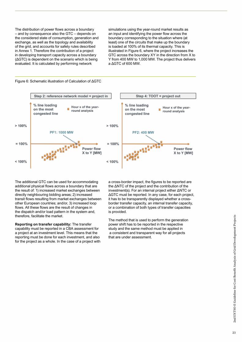
The distribution of power flows across a boundary – and by consequence also the GTC – depends on the considered state of consumption, generation and exchange, as well as the topology and availability of the grid, and accounts for safety rules described in Annex 1. Therefore the contribution of a project in developing transport capacity across a boundary (ΔGTC) is dependent on the scenario which is being evaluated. It is calculated by performing network
simulations using the year-round market results as an input and identifying the power flow across the boundary corresponding to the situation where (at least) one of the circuits that make up the boundary is loaded at 100% of its thermal capacity. This is illustrated in Figure 6, where the project increases the GTC across the boundary XY in the direction from X to Y from 400 MW to 1,000 MW. The project thus delivers a ΔGTC of 600 MW.
The additional GTC can be used for accommodating additional physical flows across a boundary that are the result of: 1) increased market exchanges between directly neighbouring bidding areas; 2) increased transit flows resulting from market exchanges between other European countries; and/or, 3) increased loop flows. All these flows are the result of changes in the dispatch and/or load pattern in the system and, therefore, facilitate the market.
Reporting on transfer capability: The transfer capability must be reported in a CBA assessment for a project at an investment level. This means that the reporting must be done for each investment, and also for the project as a whole. In the case of a project with
a cross-border impact, the figures to be reported are the ΔNTC of the project and the contribution of the investment(s). For an internal project either ΔNTC or ΔGTC must be reported. In any case, for each project, it has to be transparently displayed whether a cross-border transfer capacity, an internal transfer capacity, or a combination of both types of transfer capacities is provided.
The method that is used to perform the generation power shift has to be reported in the respective study and the same method must be applied in a consistent and transparent way for all projects that are under assessment.
Figure 6: Schematic illustration of Calculation of ΔGTC
2nd
EN
TSO
-E G
uide
line
for C
ost B
enefi
t Ana
lysi
s of
Gri
d D
evel
opm
ent P
roje
cts
24
3.2.3 Geographical scope
3.2.4 Guidelines for project NPV calculation
The main principle of system modelling is to use detailed information within the studied area, and a decreasing level of detail outside the studied area. The geographical scope of the analysis is an ENTSO-E Region at minimum, including its closest neighbours. In any case, the study area shall cover all Member States and third countries on whose territory the project shall be built, all directly neighbouring Member States and all other Member States significantly impacted by the project9.
Finally, in order to take into account the interaction of the pan-European modelled system, exchange conditions will be fixed for each of the simulation time steps, based on a global market simulation10.
Project appraisal is based hence on analyses of the global (European) increase of welfare11. This means that the goal is to bring up the projects which are the best for the European power system.
To calculate the Net Present Value of a project its monetized costs and benefits must first be estimated using the same assumptions (e.g. inflation, taxes) and then discounted such that those costs and benefits are all actualized to the time for which the assessment is needed (i.e. the year in which the study is performed). Discounted costs (negatives) and benefits (positives) can then be compared in order to calculate the NPV of the project.
The discount rates used to calculate the NPV can differ between countries, however for a fair assessment across projects a common, unique discount rate is required.
The residual value of the project at the end of the assessment period should be treated as having zero value.
The analysis period starts with the commissioning date of the project and extends to a time-frame covering the economic life12 of the assets. The period should recognise that asset economic life-spans vary depending on the technologies employed.
The following main principles shall be applied when verifying the NPV13:— Although it is acknowledged that there might be
different discount rates per country, a common discount rate needs to be used for the purpose of consistent assessments
— The economic lifetime has to consider the respective technologies (e.g. shorter lifetime for battery storage than transmission lines)
— The residual value of the project at the end of the assessment period should be treated as having zero value for the purposes of consistent analysis. It is generally recommended to study at least two horizons: one mid-term and one long-term (see Chapter 2) horizon. To evaluate projects on a common basis, benefits should be aggregated across years as follows:
— For years from year of commissioning (i.e. the start of benefits) to the first mid-term: extend the first mid-term benefits backwards
— For years between different mid-term, long-term, and very long-term (if any): linearly interpolate benefits between the time horizons
— For years beyond the farthest time horizon: maintain benefits of this farthest time horizon.
9 Annex V, §10 Regulation (EU) 347/2013.10 Within ENTSO-E, this global simulation would be based on a pan-European market data base.11 Some benefits (socio-economic welfare, CO2…) may also be disaggregated on a smaller geographical scale, like a member state or a TSO
area. This is mainly useful in the perspective of cost allocation, and should be calculated on a case by case basis, taking into account the larger variability of results across scenarios when calculating benefits related to smaller areas. In any cost allocation, due regard should be paid to compensation moneys paid under ITC (which is article 13 of Regulation 714 (see also Annex 1 for caveats on Market Power and cost allocation).
12 Economic lifetime of an asset: period over which an asset (i.e. the investments representing the project: a transmission line, a storage facility, a transformer etc.) is expected to be usable, with normal repairs and maintenance, for the purpose it was acquired, rented, or leased. Expressed usually in number of years it is usually less than the asset’s technical life, and is the period over which the asset’s depreciation is still charged.
13 See also the “Commission Implementing Regulation (EU) 2015/207” Annex III.
2nd
EN
TSO
-E G
uide
line
for C
ost B
enefi
t Ana
lysi
s of
Gri
d D
evel
opm
ent P
roje
cts
2514 More details on multi-criteria assessment and cost-benefit analysis are provided in Annex 5.
3.3
Assessment framework The assessment framework is a combined cost-benefit and multi-criteria assessment14, in line with Article 11 and Annexes IV and V of Regulation (EU) 347/2013. The criteria set out in this document have been selected on the following basis:— They enable an appreciation of project benefits
in terms of EU network objectives to:
a Ensure the development of a single European grid to permit the EU climate policy and sustainability objectives (RES, energy efficiency, CO2);
b Guarantee security of supply;
c Complete the internal energy market, especially through a contribution to increased socio-economic welfare; and
d Ensure system stability.
— They provide a measurement of project costs and feasibility (especially environmental and social viability indicated by the residual impact indicators).
— The indicators used are as simple and robust as possible. This leads to simplified methodologies for some indicators.
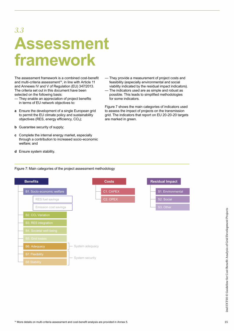
Figure 7 shows the main categories of indicators used to assess the impact of projects on the transmission grid. The indicators that report on EU 20-20-20 targets are marked in green.
Figure 7: Main categories of the project assessment methodology
Residual ImpactCostsBenefits
S2. SocialC2. OPEX RES fuel savings
Emission cost savings
B2. CO2 Variation
B3. RES integration
B4. Societal well-being
B5. Grid losses
B6. Adequacy
B7. Flexibility
B8 Stability
S1. Environmental C1. CAPEX B1. Socio-economic welfare
S3. Other
System adequacy
System security
2nd
EN
TSO
-E G
uide
line
for C
ost B
enefi
t Ana
lysi
s of
Gri
d D
evel
opm
ent P
roje
cts
26
Benefit categories are defined as follows (for a more detailed description see section 3.4):
B1. Socio-economic welfare (SEW)15 or market integration is characterised by the ability of a project to reduce congestion. It thus provides an increase in transmission capacity that makes it possible to increase commercial exchanges, so that electricity markets can trade power in a more economically efficient manner.
B2. Variation in CO2 emissions represents the change in CO2 emissions in the power system due to the project. It is a consequence of changes in generation dispatch and unlocking renewable potential. The aim to reduce CO2 emissions is explicitly included as one of the EU 20-20-20 targets and is therefore displayed as a separate indicator.
B3. RES integration: Contribution to RES integration is defined as the ability of the system to allow the connection of new RES generation, unlock existing and future “renewable” generation, and minimising curtailment of electricity produced from RES16. RES integration is one of the EU 20-20-20 targets.
B4. Variation in societal well-being as a result of variation in CO2 emissions and RES integration is the increase in societal well-being, beyond the economic effects, that are captured in the computation of SEW (indicator B1). The evolution of CO2 emissions and integration of RES in the power system due to the project are partially accounted for in the calculation of SEW. The variation of the CO2 emissions and integration of RES result in a change in variable generation costs and emission costs due to the variation in energy produced by non-zero variable cost conventional generators and the cost of emissions (e.g. carbon tax or rights under ETS) respectively, and therefore affect the system costs. However, these may not reflect the full societal benefits of having more RES in the system or the full societal cost of CO2 emissions (i.e. the damage done by emitting one tonne of CO2 is not necessarily reflected by the cost of emission certificates that producers must pay). These further effects are reported under this indicator.
B5. Variation in grid losses in the transmission grid is the cost of compensating for thermal losses in the power system due to the project. It is an indicator of energy efficiency17 and expressed as a cost in euros per year.
B6. Security of supply: Adequacy to meet demand characterises the project’s impact on the ability of a power system to provide an adequate supply of electricity to meet demand over an extended period of time. Variability of climatic effects on demand and renewable energy sources production is taken into account.
B7. Security of supply: System flexibility characterises the impact of the project on the capacity of an electric system to accommodate fast and deep changes in the net demand in the context of high penetration levels of non-dispatchable electricity generation.
B8. Security of supply: System stability characterises the project’s impact on the ability of a power system to provide a secure supply of electricity as per the technical criteria defined in Annex 1.
Residual impact is defined as follows (for a more detailed description see section 3.5):
S1. Residual environmental impact characterises the (residual) project impact as assessed through preliminary studies, and aims at giving a measure of the environmental sensitivity associated with the project.
S2. Residual social impact characterises the (residual) project impact on the (local) population affected by the project as assessed through preliminary studies, and aims at giving a measure of the social sensitivity associated with the project.
S3. Other impacts provide an indicator to capture all other impacts of a project.
These three indicators refer to the impacts that remain after impact mitigation measures have been taken. Hence, impacts that are mitigated by additional measures should no longer be listed in this category.
Costs are defined as follows (for a more detailed description see section 3.6):
C1. Capital expenditure (CAPEX). This indicator reports the capital expenditure of a project, which includes elements such as the cost of obtaining permits, conducting feasibility studies, obtaining rights-of-way, ground, preparatory work, designing, dismantling, equipment purchase and installation. CAPEX are established by analogous estimation (based on information from prior projects that are similar to the current project) and by parametric estimation (based on public information about cost of similar projects). CAPEX are expressed in euros.
C2. Operating expenditure (OPEX). These expenses are based on project operating and maintenance costs. OPEX of all projects must be given on the actual basis of the cost level with regard to the respective study year (e.g. for TYNDP the costs should be given related to 2018) and expressed in euro per year.
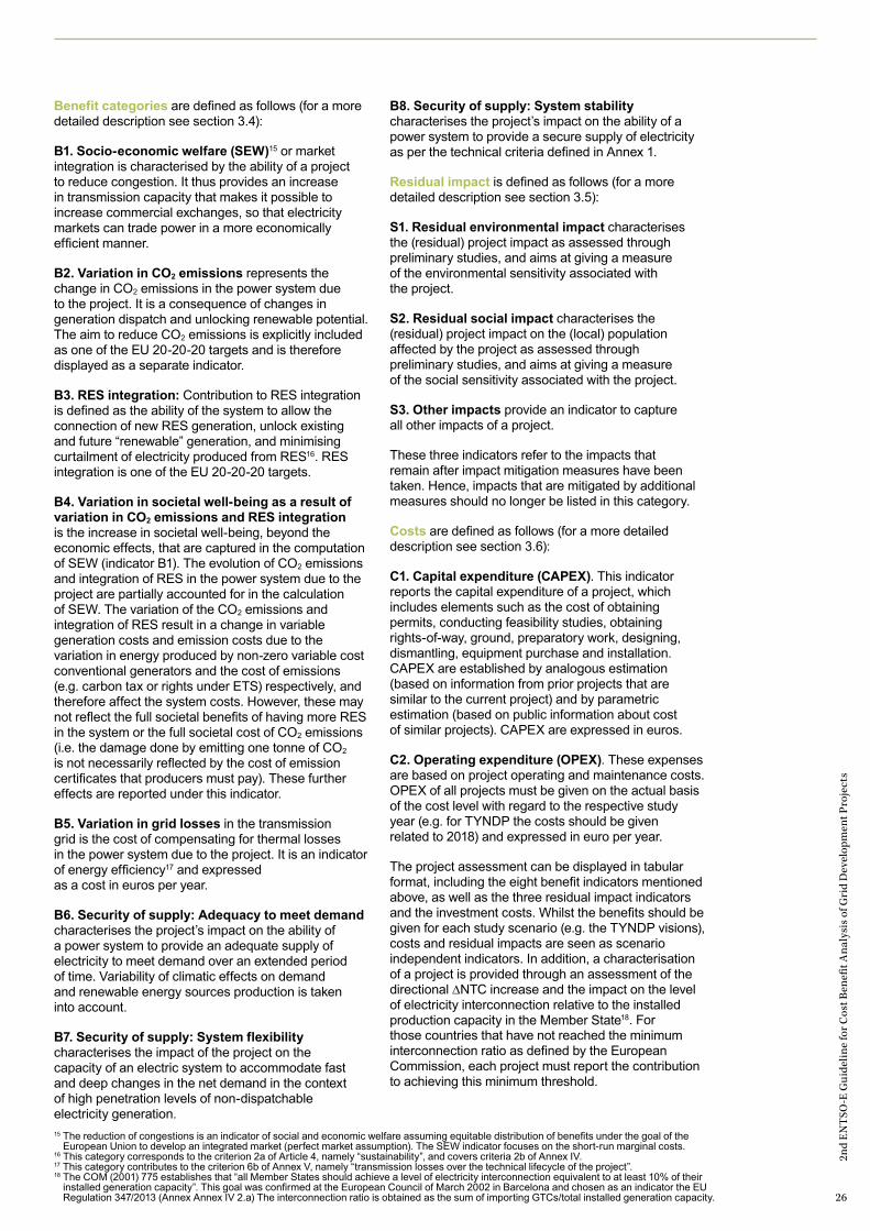
The project assessment can be displayed in tabular format, including the eight benefit indicators mentioned above, as well as the three residual impact indicators and the investment costs. Whilst the benefits should be given for each study scenario (e.g. the TYNDP visions), costs and residual impacts are seen as scenario independent indicators. In addition, a characterisation of a project is provided through an assessment of the directional ∆NTC increase and the impact on the level of electricity interconnection relative to the installed production capacity in the Member State18. For those countries that have not reached the minimum interconnection ratio as defined by the European Commission, each project must report the contribution to achieving this minimum threshold.
15 The reduction of congestions is an indicator of social and economic welfare assuming equitable distribution of benefits under the goal of the European Union to develop an integrated market (perfect market assumption). The SEW indicator focuses on the short-run marginal costs.
16 This category corresponds to the criterion 2a of Article 4, namely “sustainability”, and covers criteria 2b of Annex IV.17 This category contributes to the criterion 6b of Annex V, namely “transmission losses over the technical lifecycle of the project”.18 The COM (2001) 775 establishes that “all Member States should achieve a level of electricity interconnection equivalent to at least 10% of their
installed generation capacity”. This goal was confirmed at the European Council of March 2002 in Barcelona and chosen as an indicator the EU Regulation 347/2013 (Annex Annex IV 2.a) The interconnection ratio is obtained as the sum of importing GTCs/total installed generation capacity.
2nd
EN
TSO
-E G
uide
line
for C
ost B
enefi
t Ana
lysi
s of
Gri
d D
evel
opm
ent P
roje
cts
27
While the increased transfer capacity contribution and costs are given per investment, the benefit indicators and the residual impact indicators are provided at the project level. The contribution to transfer capacity is time and scenario dependent, but a single value should be reported for clarity reasons. This value should reflect the average transfer capacity contribution of the project.
All monetary costs and benefits shall be reported in EUR and shall be expressed in the price level of a single base year to ensure comparability. The price base year to use for reporting monetary costs and benefits shall be explicitly defined in the context of each study (e.g., €2018 in TYNDP18). ENTSO-E aims
to monetize as many indicators as possible, but the required data is not always available or monetization is the result of political preferences (e.g., the price of CO2 is dependent on future political choices, but the amount of CO2 equivalent emissions avoided by a project is not). ENTSO-E seeks to deliver a uniform and objective CBA assessment and is reluctant to publish results if their uniformity and/or objectivity cannot be guaranteed. In such cases ENTSO-E believes it is more useful to publish indicator results in their original units than to unilaterally decide on their monetary value in an arbitrary manner. The table below provides an overview of the status with regard to monetization of the indicators included in this CBA Guideline.
Indicator Original unit Monetization status
B1. SEW €/yr Monetized by default
B2. CO2 emissions
tonnes/yr Part 1: fully monetized under B1, where the effects of CO2 emissions due to the assumption with regard to emission costs are monetized and reported as additional information under indicator B1.
Part 2: this part is related to the additional societal value which is not monetized under B1.
Political CO2 reduction goals are formulated in percentages to values expressed in tonnes per year.
The magnitude of the additional monetary effect is topic of an ongoing and controversial political debate. Therefore, the CBA Methodology requires that CO2 emissions are reported separately (in tonnes).
B3. RES integration
MW or MWh/yr
Part 1: fully monetized under B1, where the effects of RES integration on SEW due to the reduction of curtailment and lower short-run variable generation costs are monetized and reported as additional information under indicator B1.
Part 2: this part is related to the additional societal value which is not monetized under B1.
Political RES integration goals are formulated and expressed in MW.
The magnitude of the additional monetary effect (on top of B1 and B2) cannot be monetised in a subjective way. Therefore, the CBA Methodology requires that RES integration is reported separately (MW or MWh/yr).
B4. Societal RES benefits
(not specified) Indicator contents are not specified. Monetization is recommended if data is available.
B5. Losses MWh/yr Monetized using yearly average electricity price per price zone.
B6. SoS – adequacy
MWh/yr Monetized, provided that VOLL-values are available. The additional adequacy margin may be conservatively monetized on the basis of investment costs in peaking units, provided that figures are available.
B7. SoS – flexibility
% (of an MW value)
Not monetized. This indicator expresses the additional capacity (NTC) in relation to existing cross-border capacity. Welfare effects arising from this are included under B1 and monetized.
B8. SoS – system stability
ordinal scale Not monetized. At present not monetized due to unavailability of quantitative models. First development is to provide quantitative model results.
Table 1: Overview of the monetization of the indicators
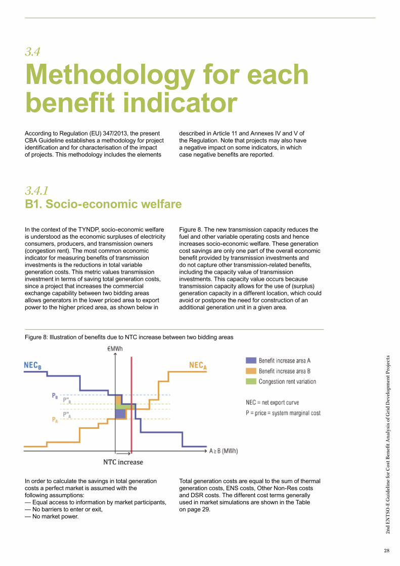
2nd
EN
TSO
-E G
uide
line
for C
ost B
enefi
t Ana
lysi
s of
Gri
d D
evel
opm
ent P
roje
cts
28
3.4.1 B1. Socio-economic welfare
In the context of the TYNDP, socio-economic welfare is understood as the economic surpluses of electricity consumers, producers, and transmission owners (congestion rent). The most common economic indicator for measuring benefits of transmission investments is the reductions in total variable generation costs. This metric values transmission investment in terms of saving total generation costs, since a project that increases the commercial exchange capability between two bidding areas allows generators in the lower priced area to export power to the higher priced area, as shown below in
Figure 8. The new transmission capacity reduces the fuel and other variable operating costs and hence increases socio-economic welfare. These generation cost savings are only one part of the overall economic benefit provided by transmission investments and do not capture other transmission-related benefits, including the capacity value of transmission investments. This capacity value occurs because transmission capacity allows for the use of (surplus) generation capacity in a different location, which could avoid or postpone the need for construction of an additional generation unit in a given area.
In order to calculate the savings in total generation costs a perfect market is assumed with the following assumptions:— Equal access to information by market participants,— No barriers to enter or exit,— No market power.
Total generation costs are equal to the sum of thermal generation costs, ENS costs, Other Non-Res costs and DSR costs. The different cost terms generally used in market simulations are shown in the Table on page 29.
3.4
Methodology for each benefit indicator According to Regulation (EU) 347/2013, the present CBA Guideline establishes a methodology for project identification and for characterisation of the impact of projects. This methodology includes the elements
described in Article 11 and Annexes IV and V of the Regulation. Note that projects may also have a negative impact on some indicators, in which case negative benefits are reported.
Figure 8: Illustration of benefits due to NTC increase between two bidding areas

2nd
EN
TSO
-E G
uide
line
for C
ost B
enefi
t Ana
lysi
s of
Gri
d D
evel
opm
ent P
roje
cts
29
In general, two different approaches can be used as a proxy for calculating the variation in socio-economic welfare:
a The generation cost approach, which compares the generation costs with and without the project for the different bidding areas.
b The total surplus approach, which compares the producer and consumer surpluses for both bidding areas, as well as the congestion rent between them, with and without the project19.
If demand is considered inelastic to price, both methods will yield the same result. If demand is considered as elastic, modelling becomes more complex. The choice of assumptions on demand elasticity and methodology of calculation of benefit from socio-economic welfare is left to ENTSO-E’s Regional Groups. Most European countries are presently considered to have price inelastic demand. However, there are various developments that appear to cause a more elastic demand-side. The development of smart grids and smart metering, as well as a growing flexibility need from the changing production technologies (more renewables, less thermal and nuclear) are drivers towards a more price-elastic demand.
There are two ways of taking into account greater flexibility of demand when assessing socio-economic welfare, the choice of the method being decided within ENTSO-E’s Regional Groups:
1 Demand is estimated through scenarios, which results in a reshaping of the demand curve (in comparison with present curves) to model the future introduction of smart grids, electric vehicles, etc. In this case, demand response is not elastic at each time step, but constitutes a shift of energy consumption from time steps with potentially high prices to time steps with potentially low prices (e.g. on the basis of hourly RES availability factors). The generation costs to supply a known demand are minimised through the generation cost approach. This assumption simplifies the complexity of the model and therefore the demand can be treated as a time series of loads that has to be met, while at the same time considering different scenarios of demand-side management.
2 Introduce hypotheses on level of price elasticity of demand. Two methods are possible:
a Using the generation cost approach, price elasticity could be taken into account via the modelling of curtailment as generators. The willingness to pay would then, for instance, be established at very high levels for domestic consumers, and at lower levels for a part of industrial demand.
b Using the total surplus method, the modelling of demand flexibility would need to be based on a quantification of the link between price and demand for each hour, allowing a correct representation of demand response in each area.
Table 2: Cost terms used in market simulations
Cost Terms in Market Simulations Description
Fuel costs Costs for fuel of thermal power plants (e.g. lignite, hard coal, natural gas etc.).
CO2-Costs Costs for CO2-emissions caused by thermal fired power plants. Depends on the power generation of thermal power plants and CO2-Price.
Start-up-costs / Shut-down costs These terms reflect the quasi-fixed costs for starting up a thermal power plant to at least a minimum power level.
Operation and maintenance costs Costs for operation and maintenance of power plants.ENS-Costs Costs for Energy not served (ENS). ENS is the expected amount
of energy not being served to consumers.DSR-Costs Costs for Demand Side Response (DSR). DSR is load demand
that can be actively changed by a certain trigger.
19 More details about how to calculate surplus are provided in Annex 6

2nd
EN
TSO
-E G
uide
line
for C
ost B
enefi
t Ana
lysi
s of
Gri
d D
evel
opm
ent P
roje
cts
30
Generation cost approachThe economic benefit is calculated from the reduction in total generation costs associated with the NTC variation created by the project. There are three aspects to this benefit:
a By reducing network bottlenecks that restrict the access of generation to the full European market, a project can reduce costs of generation restrictions, both within and between bidding areas.
b A project can contribute to reduced costs by providing a direct system connection to new, relatively low cost, generation. In the case of connection of renewables, this is also expressed by benefit B3, RES Integration.
c A project can also facilitate increased competition between generators, reducing the price of electricity to final consumers. The methods do not consider market power (see Annex 4), and as a result the expression of socio-economic welfare is the reduction in generation costs.
An economic optimisation is undertaken to determine the optimal dispatch cost of generation, with and without the project. The benefit for each case is calculated from the following relationship:
The socio-economic welfare in terms of savings in total generation costs can be calculated for internal constraints by redispatch simulations or considering virtual smaller bidding areas (with different market prices) separated by the congested internal boundary inside an official bidding area (see Annex 2). In any case it has to be transparently highlighted what method was used for the SEW calculation.
The total benefit for the horizon is calculated by summarising the benefit for all the hours of the year, which is done through market studies.
Total surplus approachThe economic benefit is calculated by adding the producer surplus (a measure of producer welfare), the consumer surplus (a measure of consumer welfare) and the congestion rents for all price areas as shown in Figure 9. The total surplus approach consists of the following three items:
a By reducing network bottlenecks, the total generation cost will be economically optimised. This is reflected in the sum of the producer surpluses that are defined as the difference between the prices the producers are willing to supply electricity and the generation costs.
b By reducing network bottlenecks that restrict the access of import from low-price areas, the total consumption cost will be decreased. This is reflected in the sum of the consumer surpluses that are defined as the difference between the prices the consumers are willing to pay for electricity and the market price.
c Finally, reducing network bottlenecks will lead to a change in total congestion rent for the TSOs.
Figure 9: Example of a new project increasing transfer capacity (ΔQ) between an export and an import region.
Benefit (for each time step) = Generation costs without the project (sum over all time steps) – Generation costs with the project (sum over all time steps)
Supply (R1)
ConsumerSurplus(R1)
ProducerSurplus(R1)
Supply (R2)
ConsumerSurplus(R2)
ProducerSurplus(R2)P1
P1’
Q1’Q1 Q2Q2’
P2P2’
Demand (R1)
Demand (R2)
Pric
e
Q (MW)
∆Q
Export Region (R1)
Pric
e
Q (MW)
Import Region (R2)
∆Q
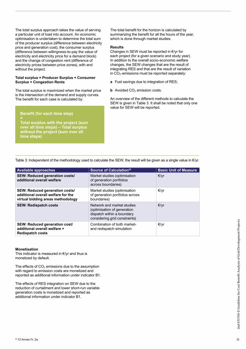
2nd
EN
TSO
-E G
uide
line
for C
ost B
enefi
t Ana
lysi
s of
Gri
d D
evel
opm
ent P
roje
cts
31
The total surplus approach takes the value of serving a particular unit of load into account. An economic optimisation is undertaken to determine the total sum of the producer surplus (difference between electricity price and generation cost), the consumer surplus (difference between willingness-to-pay the value of electricity and electricity price for a demand block) and the change of congestion rent (difference of electricity prices between price zones), with and without the project.
Total surplus = Producer Surplus + Consumer Surplus + Congestion Rents
The total surplus is maximized when the market price is the intersection of the demand and supply curves. The benefit for each case is calculated by:
The total benefit for the horizon is calculated by summarizing the benefit for all the hours of the year, which is done through market studies.
ResultsChanges in SEW must be reported in €/yr for each project (for a given scenario and study year). In addition to the overall socio-economic welfare changes, the SEW changes that are the result of integrating RES and that are the result of variation in CO2-emissions must be reported separately:
a Fuel savings due to integration of RES;
b Avoided CO2 emission costs.
An overview of the different methods to calculate the SEW is given in Table 3. It shall be noted that only one value for SEW will be reported.
MonetisationThis indicator is measured in €/yr and thus is monetized by default.
The effects of CO2 emissions due to the assumption with regard to emission costs are monetized and reported as additional information under indicator B1.
The effects of RES integration on SEW due to the reduction of curtailment and lower short-run variable generation costs is monetized and reported as additional information under indicator B1.
Table 3: Independent of the methodology used to calculate the SEW, the result will be given as a single value in €/yr.
Available approaches Source of Calculation20 Basic Unit of Measure
SEW: Reduced generation costs/ additional overall welfare
Market studies (optimisation of generation portfolios across boundaries)
€/yr
SEW: Reduced generation costs/ additional overall welfare for the virtual bidding areas methodology
Market studies (optimisation of generation portfolios across boundaries)
€/yr
SEW: Redispatch costs Network and market studies (optimisation of generation dispatch within a boundary considering grid constraints)
€/yr
SEW: Reduced generation cost/ additional overall welfare + Redispatch costs
Combination of both market- and redispatch simulation
€/yr
Benefit (for each time step) = Total surplus with the project (sum over all time steps) – Total surplus without the project (sum over all time steps)
20 Cf Annex IV, 2a.
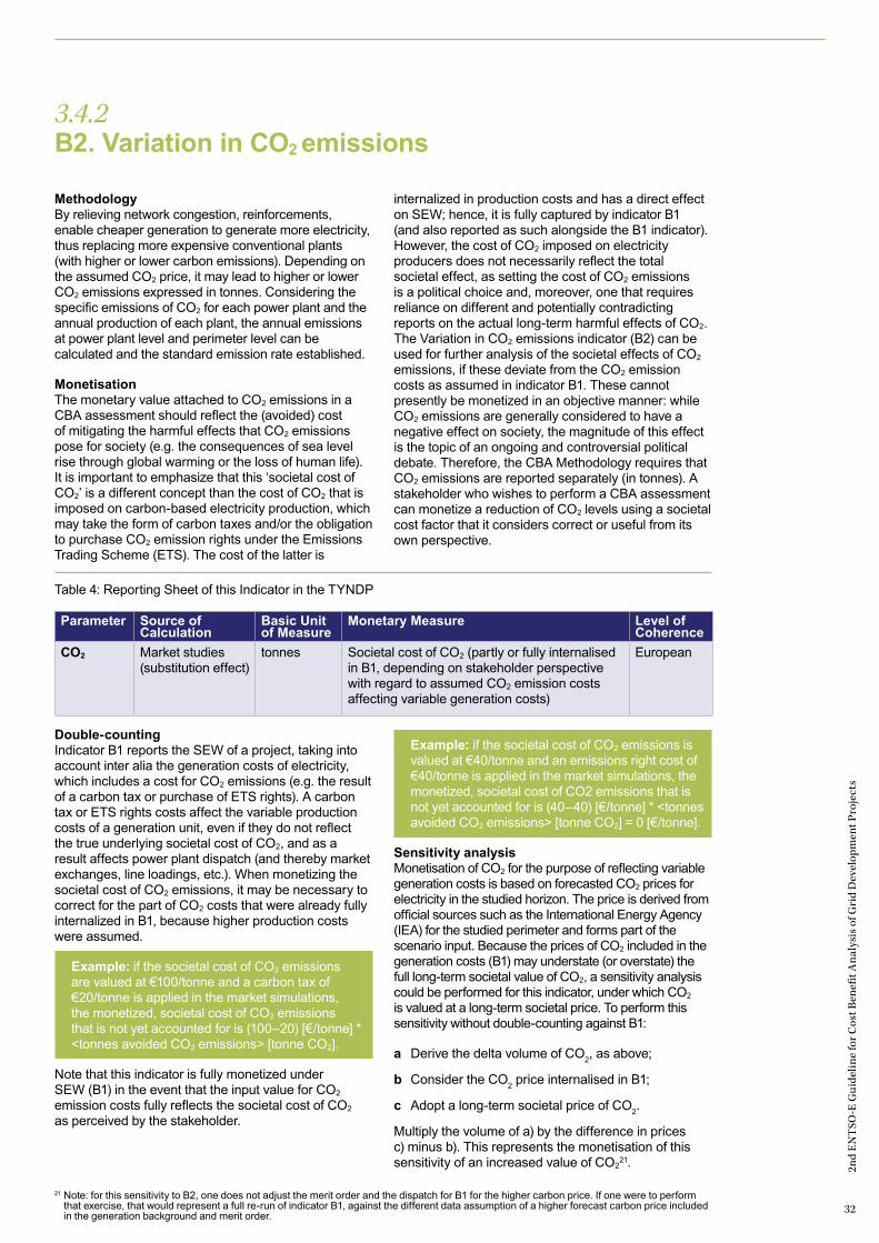
2nd
EN
TSO
-E G
uide
line
for C
ost B
enefi
t Ana
lysi
s of
Gri
d D
evel
opm
ent P
roje
cts
32
Table 4: Reporting Sheet of this Indicator in the TYNDP
Parameter Source of Calculation
Basic Unit of Measure
Monetary Measure Level of Coherence
CO2 Market studies (substitution effect)
tonnes Societal cost of CO2 (partly or fully internalised in B1, depending on stakeholder perspective with regard to assumed CO2 emission costs affecting variable generation costs)
European
3.4.2 B2. Variation in CO2 emissions
MethodologyBy relieving network congestion, reinforcements, enable cheaper generation to generate more electricity, thus replacing more expensive conventional plants (with higher or lower carbon emissions). Depending on the assumed CO2 price, it may lead to higher or lower CO2 emissions expressed in tonnes. Considering the specific emissions of CO2 for each power plant and the annual production of each plant, the annual emissions at power plant level and perimeter level can be calculated and the standard emission rate established.
MonetisationThe monetary value attached to CO2 emissions in a CBA assessment should reflect the (avoided) cost of mitigating the harmful effects that CO2 emissions pose for society (e.g. the consequences of sea level rise through global warming or the loss of human life). It is important to emphasize that this ‘societal cost of CO2’ is a different concept than the cost of CO2 that is imposed on carbon-based electricity production, which may take the form of carbon taxes and/or the obligation to purchase CO2 emission rights under the Emissions Trading Scheme (ETS). The cost of the latter is
internalized in production costs and has a direct effect on SEW; hence, it is fully captured by indicator B1 (and also reported as such alongside the B1 indicator). However, the cost of CO2 imposed on electricity producers does not necessarily reflect the total societal effect, as setting the cost of CO2 emissions is a political choice and, moreover, one that requires reliance on different and potentially contradicting reports on the actual long-term harmful effects of CO2. The Variation in CO2 emissions indicator (B2) can be used for further analysis of the societal effects of CO2 emissions, if these deviate from the CO2 emission costs as assumed in indicator B1. These cannot presently be monetized in an objective manner: while CO2 emissions are generally considered to have a negative effect on society, the magnitude of this effect is the topic of an ongoing and controversial political debate. Therefore, the CBA Methodology requires that CO2 emissions are reported separately (in tonnes). A stakeholder who wishes to perform a CBA assessment can monetize a reduction of CO2 levels using a societal cost factor that it considers correct or useful from its own perspective.
Double-countingIndicator B1 reports the SEW of a project, taking into account inter alia the generation costs of electricity, which includes a cost for CO2 emissions (e.g. the result of a carbon tax or purchase of ETS rights). A carbon tax or ETS rights costs affect the variable production costs of a generation unit, even if they do not reflect the true underlying societal cost of CO2, and as a result affects power plant dispatch (and thereby market exchanges, line loadings, etc.). When monetizing the societal cost of CO2 emissions, it may be necessary to correct for the part of CO2 costs that were already fully internalized in B1, because higher production costs were assumed.
Example: if the societal cost of CO2 emissions are valued at €100/tonne and a carbon tax of €20/tonne is applied in the market simulations, the monetized, societal cost of CO2 emissions that is not yet accounted for is (100–20) [€/tonne] * <tonnes avoided CO2 emissions> [tonne CO2].
Note that this indicator is fully monetized under SEW (B1) in the event that the input value for CO2 emission costs fully reflects the societal cost of CO2 as perceived by the stakeholder.
Example: if the societal cost of CO2 emissions is valued at €40/tonne and an emissions right cost of €40/tonne is applied in the market simulations, the monetized, societal cost of CO2 emissions that is not yet accounted for is (40–40) [€/tonne] * <tonnes avoided CO2 emissions> [tonne CO2] = 0 [€/tonne].
Sensitivity analysisMonetisation of CO2 for the purpose of reflecting variable generation costs is based on forecasted CO2 prices for electricity in the studied horizon. The price is derived from official sources such as the International Energy Agency (IEA) for the studied perimeter and forms part of the scenario input. Because the prices of CO2 included in the generation costs (B1) may understate (or overstate) the full long-term societal value of CO2, a sensitivity analysis could be performed for this indicator, under which CO2 is valued at a long-term societal price. To perform this sensitivity without double-counting against B1:
a Derive the delta volume of CO2, as above;
b Consider the CO2 price internalised in B1;
c Adopt a long-term societal price of CO2.
Multiply the volume of a) by the difference in prices c) minus b). This represents the monetisation of this sensitivity of an increased value of CO2
21.
21 Note: for this sensitivity to B2, one does not adjust the merit order and the dispatch for B1 for the higher carbon price. If one were to perform that exercise, that would represent a full re-run of indicator B1, against the different data assumption of a higher forecast carbon price included in the generation background and merit order.
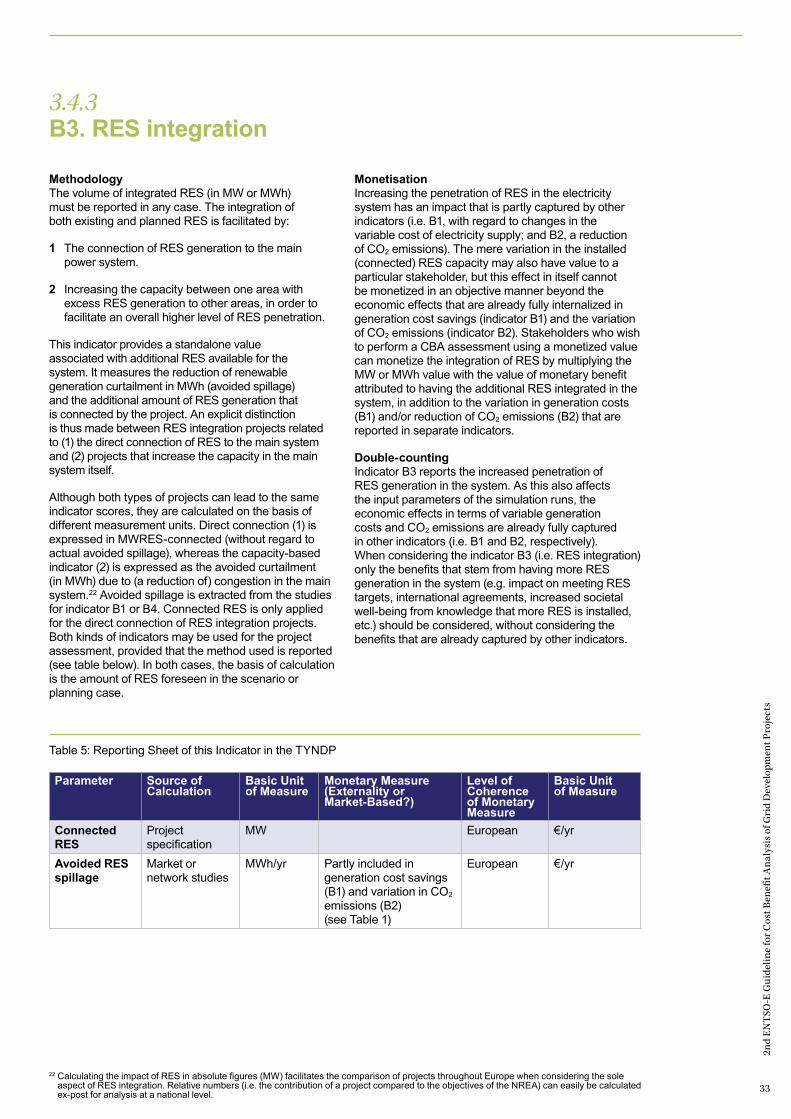
2nd
EN
TSO
-E G
uide
line
for C
ost B
enefi
t Ana
lysi
s of
Gri
d D
evel
opm
ent P
roje
cts
33
3.4.3 B3. RES integration
MethodologyThe volume of integrated RES (in MW or MWh) must be reported in any case. The integration of both existing and planned RES is facilitated by:
1 The connection of RES generation to the main power system.
2 Increasing the capacity between one area with excess RES generation to other areas, in order to facilitate an overall higher level of RES penetration.
This indicator provides a standalone value associated with additional RES available for the system. It measures the reduction of renewable generation curtailment in MWh (avoided spillage) and the additional amount of RES generation that is connected by the project. An explicit distinction is thus made between RES integration projects related to (1) the direct connection of RES to the main system and (2) projects that increase the capacity in the main system itself.
Although both types of projects can lead to the same indicator scores, they are calculated on the basis of different measurement units. Direct connection (1) is expressed in MWRES-connected (without regard to actual avoided spillage), whereas the capacity-based indicator (2) is expressed as the avoided curtailment (in MWh) due to (a reduction of) congestion in the main system.22 Avoided spillage is extracted from the studies for indicator B1 or B4. Connected RES is only applied for the direct connection of RES integration projects. Both kinds of indicators may be used for the project assessment, provided that the method used is reported (see table below). In both cases, the basis of calculation is the amount of RES foreseen in the scenario or planning case.
MonetisationIncreasing the penetration of RES in the electricity system has an impact that is partly captured by other indicators (i.e. B1, with regard to changes in the variable cost of electricity supply; and B2, a reduction of CO2 emissions). The mere variation in the installed (connected) RES capacity may also have value to a particular stakeholder, but this effect in itself cannot be monetized in an objective manner beyond the economic effects that are already fully internalized in generation cost savings (indicator B1) and the variation of CO2 emissions (indicator B2). Stakeholders who wish to perform a CBA assessment using a monetized value can monetize the integration of RES by multiplying the MW or MWh value with the value of monetary benefit attributed to having the additional RES integrated in the system, in addition to the variation in generation costs (B1) and/or reduction of CO2 emissions (B2) that are reported in separate indicators.
Double-countingIndicator B3 reports the increased penetration of RES generation in the system. As this also affects the input parameters of the simulation runs, the economic effects in terms of variable generation costs and CO2 emissions are already fully captured in other indicators (i.e. B1 and B2, respectively). When considering the indicator B3 (i.e. RES integration) only the benefits that stem from having more RES generation in the system (e.g. impact on meeting RES targets, international agreements, increased societal well-being from knowledge that more RES is installed, etc.) should be considered, without considering the benefits that are already captured by other indicators.
22 Calculating the impact of RES in absolute figures (MW) facilitates the comparison of projects throughout Europe when considering the sole aspect of RES integration. Relative numbers (i.e. the contribution of a project compared to the objectives of the NREA) can easily be calculated ex-post for analysis at a national level.
Table 5: Reporting Sheet of this Indicator in the TYNDP
Parameter Source of Calculation
Basic Unit of Measure
Monetary Measure (Externality or Market-Based?)
Level of Coherence of Monetary Measure
Basic Unit of Measure
Connected RES
Project specification
MW European €/yr
Avoided RES spillage
Market or network studies
MWh/yr Partly included in generation cost savings (B1) and variation in CO2 emissions (B2) (see Table 1)
European €/yr
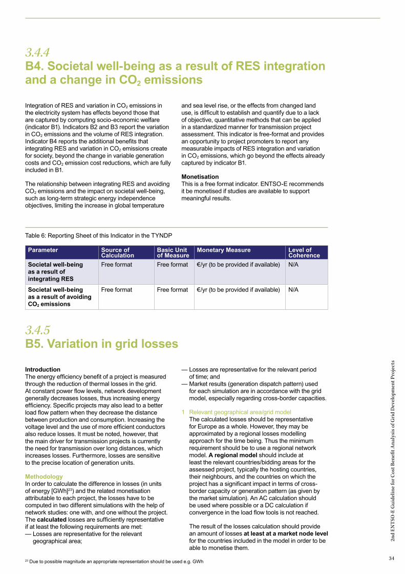
2nd
EN
TSO
-E G
uide
line
for C
ost B
enefi
t Ana
lysi
s of
Gri
d D
evel
opm
ent P
roje
cts
34
Table 6: Reporting Sheet of this Indicator in the TYNDP
Parameter Source of Calculation
Basic Unit of Measure
Monetary Measure Level of Coherence
Societal well-being as a result of integrating RES
Free format Free format €/yr (to be provided if available) N/A
Societal well-being as a result of avoiding CO2 emissions
Free format Free format €/yr (to be provided if available) N/A
3.4.4 B4. Societal well-being as a result of RES integration and a change in CO2 emissions
Integration of RES and variation in CO2 emissions in the electricity system has effects beyond those that are captured by computing socio-economic welfare (indicator B1). Indicators B2 and B3 report the variation in CO2 emissions and the volume of RES integration. Indicator B4 reports the additional benefits that integrating RES and variation in CO2 emissions create for society, beyond the change in variable generation costs and CO2 emission cost reductions, which are fully included in B1.
The relationship between integrating RES and avoiding CO2 emissions and the impact on societal well-being, such as long-term strategic energy independence objectives, limiting the increase in global temperature
and sea level rise, or the effects from changed land use, is difficult to establish and quantify due to a lack of objective, quantitative methods that can be applied in a standardized manner for transmission project assessment. This indicator is free-format and provides an opportunity to project promoters to report any measurable impacts of RES integration and variation in CO2 emissions, which go beyond the effects already captured by indicator B1.
MonetisationThis is a free format indicator. ENTSO-E recommends it be monetised if studies are available to support meaningful results.
3.4.5 B5. Variation in grid losses
IntroductionThe energy efficiency benefit of a project is measured through the reduction of thermal losses in the grid. At constant power flow levels, network development generally decreases losses, thus increasing energy efficiency. Specific projects may also lead to a better load flow pattern when they decrease the distance between production and consumption. Increasing the voltage level and the use of more efficient conductors also reduce losses. It must be noted, however, that the main driver for transmission projects is currently the need for transmission over long distances, which increases losses. Furthermore, losses are sensitive to the precise location of generation units.
MethodologyIn order to calculate the difference in losses (in units of energy [GWh]23) and the related monetisation attributable to each project, the losses have to be computed in two different simulations with the help of network studies: one with, and one without the project. The calculated losses are sufficiently representative if at least the following requirements are met:— Losses are representative for the relevant
geographical area;
— Losses are representative for the relevant period of time; and
— Market results (generation dispatch pattern) used for each simulation are in accordance with the grid model, especially regarding cross-border capacities.
1 Relevant geographical area/grid model The calculated losses should be representative
for Europe as a whole. However, they may be approximated by a regional losses modelling approach for the time being. Thus the minimum requirement should be to use a regional network model. A regional model should include at least the relevant countries/bidding areas for the assessed project, typically the hosting countries, their neighbours, and the countries on which the project has a significant impact in terms of cross-border capacity or generation pattern (as given by the market simulation). An AC calculation should be used where possible or a DC calculation if convergence in the load flow tools is not reached.
The result of the losses calculation should provide an amount of losses at least at a market node level for the countries included in the model in order to be able to monetise them.
23 Due to possible magnitude an appropriate representation should be used e.g. GWh
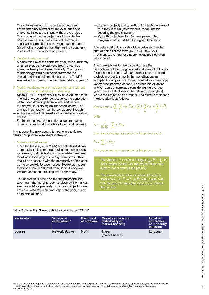
2nd
EN
TSO
-E G
uide
line
for C
ost B
enefi
t Ana
lysi
s of
Gri
d D
evel
opm
ent P
roje
cts
35
Parameter Source of calculation25
Basic unit of measure
Monetary measure (externality or market-based?)
Level of coherence of monetary measure
Losses Network studies MWh €/year (market-based)
European
The sole losses occurring on the project itself are deemed not relevant for the evaluation of a difference in losses with and without the project. This is true, since the project would modify the flow pattern on other lines due to the change in impedances, and due to a new generation pattern (also in other countries than the hosting countries), in case of a RES connection project.
2 Relevant period of time A calculation over the complete year, with sufficiently
small time steps (typically one hour), should be aimed as being the closest to reality. The chosen methodology must be representative for the considered period of time (in the current TYNDP scenarios this means one complete calendar year).24
3 Market results/generation pattern with and without the project or in grid stressed situations
Since a TYNDP project will likely have an impact on internal or cross-border congestions, the generation pattern can differ significantly with and without the project, thus having an impact on losses. The change in generation can be considered through:
— A change in the NTC used for the market simulation, and/or
— For internal projects/generation accommodation projects, a re-dispatch methodology could be used.
In any case, the new generation pattern should not cause congestions elsewhere in the grid.
4 Monetisation of losses Once the losses (i.e. in MWh) are calculated, it can
be monetised. It is important, when monetisation is performed, that this is done in a consistent manner for all assessed projects. In a general sense, this should be assessed with the perspective of the cost borne by society to cover losses. However, the cost for losses here is different from Social-Economic-Welfare and should be displayed separately.
The approach is based on market prices that are taken from the marginal cost as given by the market simulation. More precisely, for a given project losses are calculated for each time step of the year, h, and each market zone, i:
— p’h,i (with project) and ph,i (without project) the amount of losses in MWh (after eventual measures for securing the grid situation);
— s’h,i (with project) and sh,i (without project) the marginal costs in €/MWh for a given time step.
The delta cost of losses should be calculated as the sum of h and i of the term (p’h,i * s’h,i) – (ph,i * sh,i). In this case, eventual re-dispatch costs are not taken into account.
The prerequisites for the calculation are the computation of the marginal cost and amount of losses for each market zone, with and without the assessed project. In order to simplify the monetisation, an acceptable compromise should be used as an average yearly price per market zone. The variation of losses in MWh can be monetised considering the average yearly price of electricity in the relevant country(ies) where the project has an impact. The formula for losses monetisation is as follows:
i i ih h
Yearly cost C =∑ ∑ sh,i Ph,i ≈∑ si ∑Ph,i ≈ ∑ si Pi
With:
— The variation in losses in energy is ∑ i P’i – ∑ i Pi (total system losses with the project minus total system losses without the project)
— The monetisation of the variation of losses is therefore ∑ i s’ i P’i – ∑ i si Pi (total losses cost with the project minus total losses cost without the project)
24 As a provisional exception, a computation of losses based on definite point in times can be used in order to approximate year-round losses. In such case, the chosen point in times should be numerous enough to ensure representativeness, and weighted in a correct manner.
25 Cf Annex IV, 2c.
Table 7: Reporting Sheet of this Indicator in the TYNDP
1 8760 ∑ h sh,i
(the yearly average spot price for the price area, i)
si =
∑ h Ph,i
(the yearly average spot price for the price area, i)
Pi =

2nd
EN
TSO
-E G
uide
line
for C
ost B
enefi
t Ana
lysi
s of
Gri
d D
evel
opm
ent P
roje
cts
36
3.4.6 B6. Security of supply: adequacy to meet demand
Adequacy to meet demand is the ability of a power system to provide an adequate supply of electricity in order to meet the demand at any moment in time, i.e. that a sufficient volume of power is available and can be physically delivered to consumers during all time steps (e.g. hours). In achieving this objective, generation and transmission capacity are complementary elements: generation capacity requires a transmission grid for power to flow from generation source to load. This is particularly relevant in the context of geo-temporal fluctuations in intermittent renewable energy sources, which may require certain areas to depend on generation that is only available in other areas at a certain moment.
Transmission capacity makes it possible to meet demand in one area with generation capacity that is located in another area. Generation investment, transmission investments, and government policies affecting the developments in these cause effects upon each other. If there is sufficient generation capacity in a given area to meet demand at all times, constructing additional transmission capacity will not lead to a reduction of lost load. Notwithstanding, the availability of transmission capacity increases security of supply in that region, because it increases the adequacy margin by providing access to generation sources that are physically located elsewhere. If the generation and load profiles of multiple areas are different (e.g. different RES availability), spare generation capacity may be shared across regions allowing for a more efficient use of installed generation capacity. Hence, transmission capacity increases the adequacy margin by enabling the use of (surplus) generation capacity that is located in a different location. This is a substitute for the construction of additional generation capacity in a given area.
Generation adequacy is expressed using two sub-indicators, with the aim to capture security of supply issues as well as the contribution of transmission capacity to the efficiency of spare generation capacity:— Expected Energy Not Served (EENS) [MWh]: to
capture the benefit of the project in case there is a security of supply issue detected;
— Additional adequacy margin [MW]: to capture the benefit of the project if EENS equals 0 MWh26.
EENS: EENS may be calculated using market or network models, depending on the type of contribution of the transmission project under consideration. If bidding areas rely on other bidding areas during some time steps of the year to meet demand, the market simulations will show EENS in these time steps if the market is unable to supply this power (e.g. due to insufficient transmission capacity). If a transmission project reduces a loss of load within bidding zones, network simulations can be used to reveal the contribution of the project to reducing EENS.
Additional adequacy margin: The Additional adequacy margin is calculated using year-round market simulations (i.e. 8760 hours per year). In each time step a certain proportion of the available generation capacity is used in different bidding areas. This represents the level of required installed generation capacity. Comparing two model runs (with and without the project) result in different values, and indicate the contribution of the transmission project to reduce the required installed generation capacity (while maintaining the same level of EENS of 0 MWh/yr).
The ‘Additional adequacy margin’ provides information on the contribution of a project to share the available generation resources in different locations. The contribution of a transmission project to reducing EENS is highly sensitive to the scenario parameters with regard to installed (available) generation capacity. If relatively large volumes of conventional generation capacity are assumed available, there will be no EENS regardless of whether the transmission project is realized. The ‘Additional adequacy margin’ indicator seeks to capture the contribution of a project to facilitating the system’s adequacy to meet demand, even if there is no critical security of supply issue given the choice of scenario parameters. Such a gain in adequacy can be obtained by building a transmission link, because generation capacity that is unused at a given moment in time in one area becomes available for supply to another area. This may create a system-wide benefit if the patterns of demand, variable renewables availability, and unit maintenance are different throughout the system. This is illustrated in the example provided on page 37.
26 As already mentioned the EENS indicator is highly correlated to the chosen scenario, the occurrence of EENS equals 0 MWh are likely in cases where the scenarios are not ‘extreme enough’. In this case also a clear explanation can be given why the EENS equals zero.
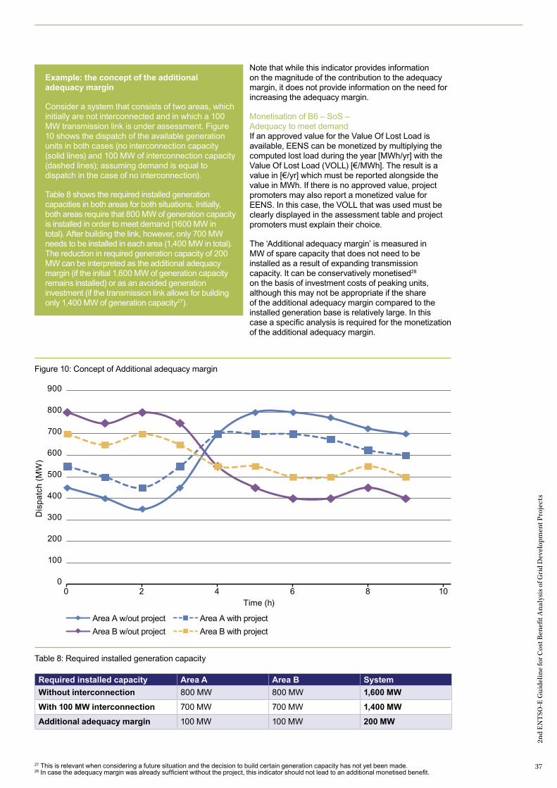
2nd
EN
TSO
-E G
uide
line
for C
ost B
enefi
t Ana
lysi
s of
Gri
d D
evel
opm
ent P
roje
cts
37
Example: the concept of the additional adequacy margin
Consider a system that consists of two areas, which initially are not interconnected and in which a 100 MW transmission link is under assessment. Figure 10 shows the dispatch of the available generation units in both cases (no interconnection capacity (solid lines) and 100 MW of interconnection capacity (dashed lines); assuming demand is equal to dispatch in the case of no interconnection).
Table 8 shows the required installed generation capacities in both areas for both situations. Initially, both areas require that 800 MW of generation capacity is installed in order to meet demand (1600 MW in total). After building the link, however, only 700 MW needs to be installed in each area (1,400 MW in total). The reduction in required generation capacity of 200 MW can be interpreted as the additional adequacy margin (if the initial 1,600 MW of generation capacity remains installed) or as an avoided generation investment (if the transmission link allows for building only 1,400 MW of generation capacity27).
Note that while this indicator provides information on the magnitude of the contribution to the adequacy margin, it does not provide information on the need for increasing the adequacy margin.
Monetisation of B6 – SoS – Adequacy to meet demandIf an approved value for the Value Of Lost Load is available, EENS can be monetized by multiplying the computed lost load during the year [MWh/yr] with the Value Of Lost Load (VOLL) [€/MWh]. The result is a value in [€/yr] which must be reported alongside the value in MWh. If there is no approved value, project promoters may also report a monetized value for EENS. In this case, the VOLL that was used must be clearly displayed in the assessment table and project promoters must explain their choice.
The ‘Additional adequacy margin’ is measured in MW of spare capacity that does not need to be installed as a result of expanding transmission capacity. It can be conservatively monetised28 on the basis of investment costs of peaking units, although this may not be appropriate if the share of the additional adequacy margin compared to the installed generation base is relatively large. In this case a specific analysis is required for the monetization of the additional adequacy margin.
27 This is relevant when considering a future situation and the decision to build certain generation capacity has not yet been made.28 In case the adequacy margin was already sufficient without the project, this indicator should not lead to an additional monetised benefit.
Figure 10: Concept of Additional adequacy margin
Required installed capacity Area A Area B System
Without interconnection 800 MW 800 MW 1,600 MW
With 100 MW interconnection 700 MW 700 MW 1,400 MW
Additional adequacy margin 100 MW 100 MW 200 MW
Table 8: Required installed generation capacity
Area A w/out project Area A with projectArea B w/out project Area B with project
0
100
200
300
400
500
600
700
800
900
Dis
patc
h (M
W)
0 2Time (h)
4 106 8
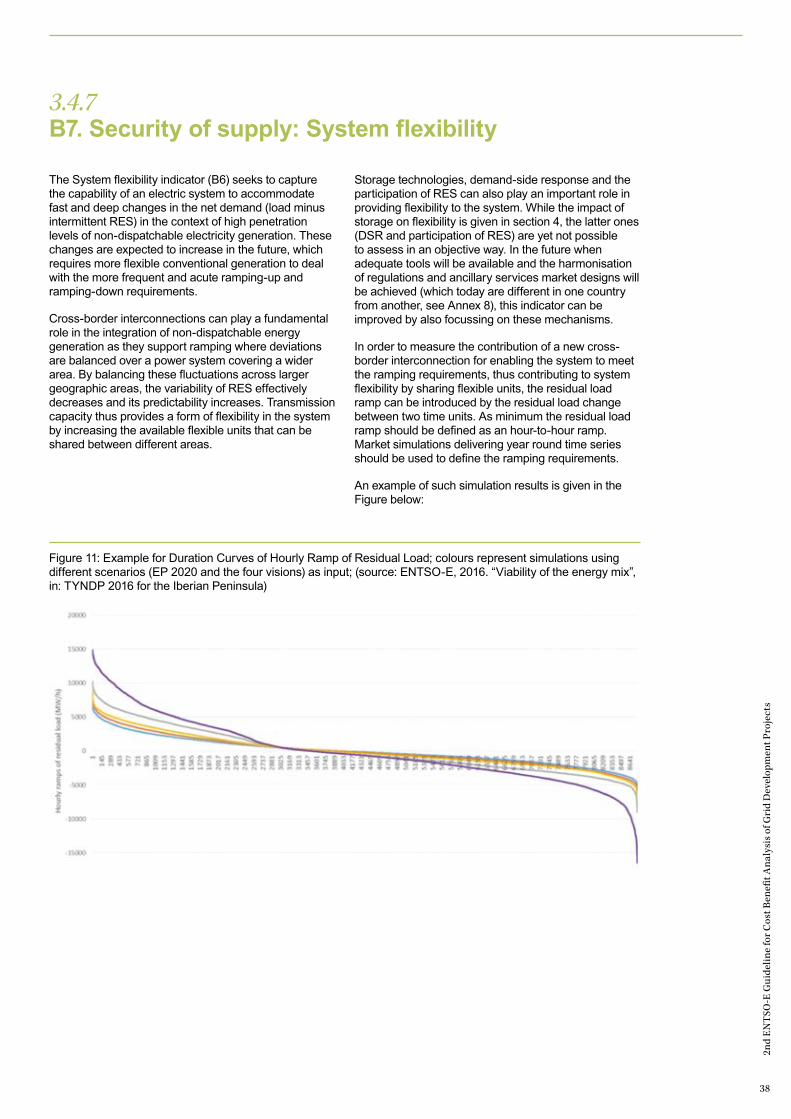
2nd
EN
TSO
-E G
uide
line
for C
ost B
enefi
t Ana
lysi
s of
Gri
d D
evel
opm
ent P
roje
cts
38
3.4.7 B7. Security of supply: System flexibility
The System flexibility indicator (B6) seeks to capture the capability of an electric system to accommodate fast and deep changes in the net demand (load minus intermittent RES) in the context of high penetration levels of non-dispatchable electricity generation. These changes are expected to increase in the future, which requires more flexible conventional generation to deal with the more frequent and acute ramping-up and ramping-down requirements.
Cross-border interconnections can play a fundamental role in the integration of non-dispatchable energy generation as they support ramping where deviations are balanced over a power system covering a wider area. By balancing these fluctuations across larger geographic areas, the variability of RES effectively decreases and its predictability increases. Transmission capacity thus provides a form of flexibility in the system by increasing the available flexible units that can be shared between different areas.
Storage technologies, demand-side response and the participation of RES can also play an important role in providing flexibility to the system. While the impact of storage on flexibility is given in section 4, the latter ones (DSR and participation of RES) are yet not possible to assess in an objective way. In the future when adequate tools will be available and the harmonisation of regulations and ancillary services market designs will be achieved (which today are different in one country from another, see Annex 8), this indicator can be improved by also focussing on these mechanisms.
In order to measure the contribution of a new cross-border interconnection for enabling the system to meet the ramping requirements, thus contributing to system flexibility by sharing flexible units, the residual load ramp can be introduced by the residual load change between two time units. As minimum the residual load ramp should be defined as an hour-to-hour ramp. Market simulations delivering year round time series should be used to define the ramping requirements.
An example of such simulation results is given in the Figure below:
Figure 11: Example for Duration Curves of Hourly Ramp of Residual Load; colours represent simulations using different scenarios (EP 2020 and the four visions) as input; (source: ENTSO-E, 2016. “Viability of the energy mix”, in: TYNDP 2016 for the Iberian Peninsula)
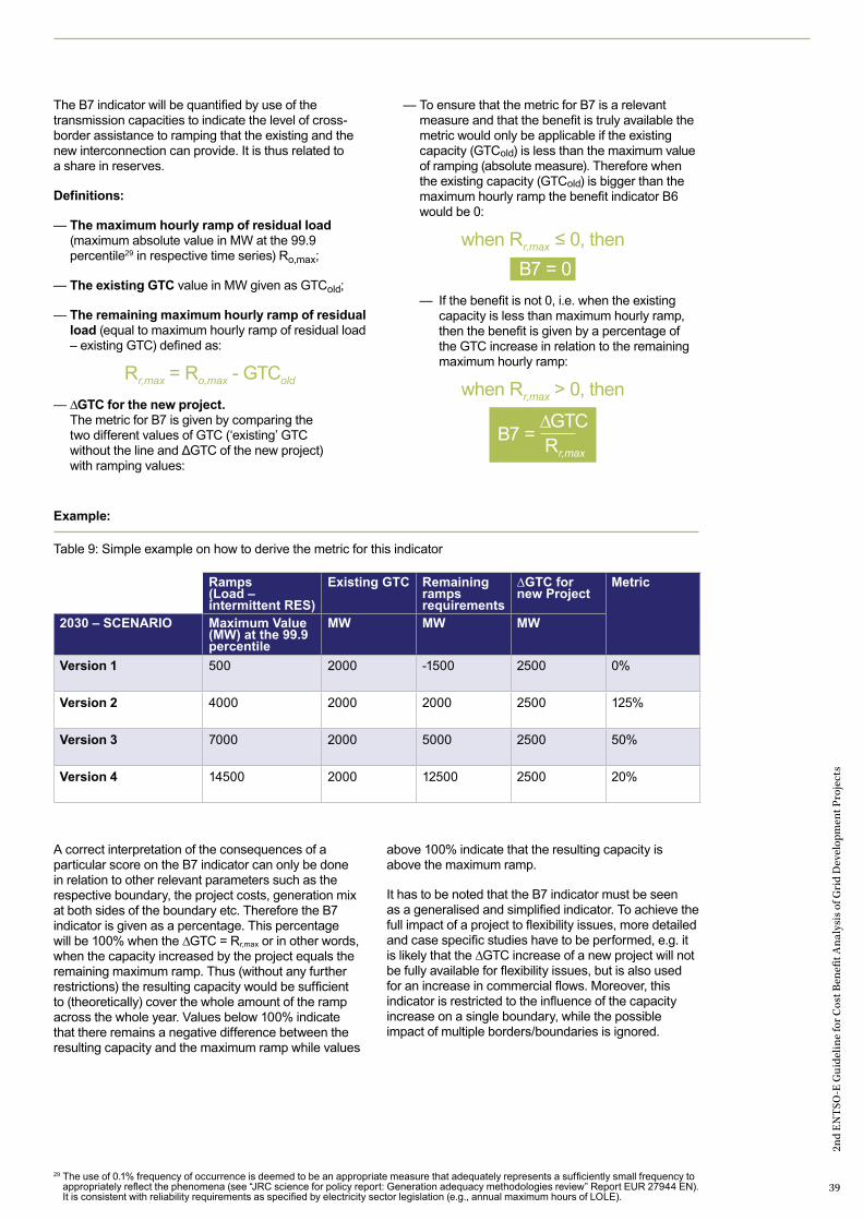
2nd
EN
TSO
-E G
uide
line
for C
ost B
enefi
t Ana
lysi
s of
Gri
d D
evel
opm
ent P
roje
cts
39
The B7 indicator will be quantified by use of the transmission capacities to indicate the level of cross-border assistance to ramping that the existing and the new interconnection can provide. It is thus related to a share in reserves.
Definitions:
— The maximum hourly ramp of residual load (maximum absolute value in MW at the 99.9 percentile29 in respective time series) Ro,max;
— The existing GTC value in MW given as GTCold;
— The remaining maximum hourly ramp of residual load (equal to maximum hourly ramp of residual load – existing GTC) defined as:
Rr,max = Ro,max - GTCold
— ΔGTC for the new project. The metric for B7 is given by comparing the
two different values of GTC (‘existing’ GTC without the line and ΔGTC of the new project) with ramping values:
— To ensure that the metric for B7 is a relevant measure and that the benefit is truly available the metric would only be applicable if the existing capacity (GTCold) is less than the maximum value of ramping (absolute measure). Therefore when the existing capacity (GTCold) is bigger than the maximum hourly ramp the benefit indicator B6 would be 0:
when Rr,max ≤ 0, then B7 = 0
— If the benefit is not 0, i.e. when the existing capacity is less than maximum hourly ramp, then the benefit is given by a percentage of the GTC increase in relation to the remaining maximum hourly ramp:
when Rr,max > 0, then
B7 = ∆GTC
Rr,max
A correct interpretation of the consequences of a particular score on the B7 indicator can only be done in relation to other relevant parameters such as the respective boundary, the project costs, generation mix at both sides of the boundary etc. Therefore the B7 indicator is given as a percentage. This percentage will be 100% when the ∆GTC = Rr,max or in other words, when the capacity increased by the project equals the remaining maximum ramp. Thus (without any further restrictions) the resulting capacity would be sufficient to (theoretically) cover the whole amount of the ramp across the whole year. Values below 100% indicate that there remains a negative difference between the resulting capacity and the maximum ramp while values
above 100% indicate that the resulting capacity is above the maximum ramp.
It has to be noted that the B7 indicator must be seen as a generalised and simplified indicator. To achieve the full impact of a project to flexibility issues, more detailed and case specific studies have to be performed, e.g. it is likely that the ∆GTC increase of a new project will not be fully available for flexibility issues, but is also used for an increase in commercial flows. Moreover, this indicator is restricted to the influence of the capacity increase on a single boundary, while the possible impact of multiple borders/boundaries is ignored.
Parameter Ramps (Load – intermittent RES)
Existing GTC Remaining ramps requirements
ΔGTC for new Project
Metric
2030 – SCENARIO Maximum Value (MW) at the 99.9 percentile
MW MW MW
Version 1 500 2000 -1500 2500 0%
Version 2 4000 2000 2000 2500 125%
Version 3 7000 2000 5000 2500 50%
Version 4 14500 2000 12500 2500 20%
Table 9: Simple example on how to derive the metric for this indicator
29 The use of 0.1% frequency of occurrence is deemed to be an appropriate measure that adequately represents a sufficiently small frequency to appropriately reflect the phenomena (see “JRC science for policy report: Generation adequacy methodologies review” Report EUR 27944 EN). It is consistent with reliability requirements as specified by electricity sector legislation (e.g., annual maximum hours of LOLE).
Example:
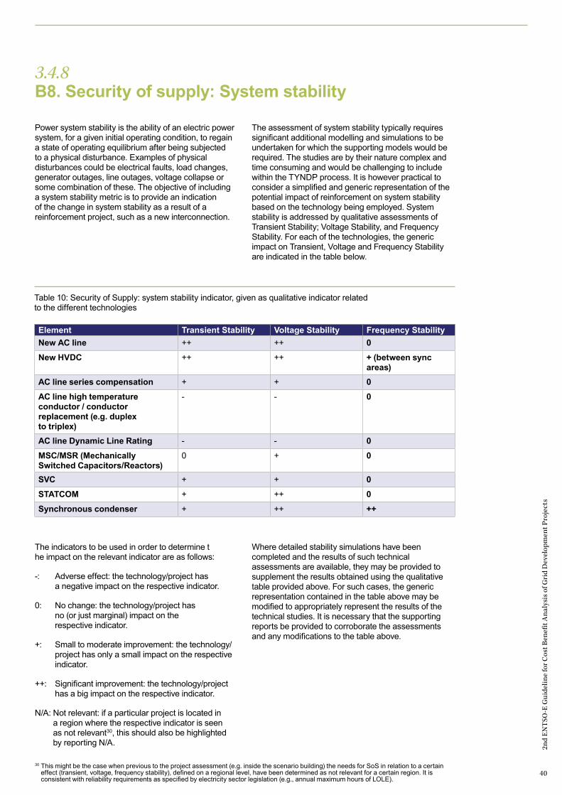
2nd
EN
TSO
-E G
uide
line
for C
ost B
enefi
t Ana
lysi
s of
Gri
d D
evel
opm
ent P
roje
cts
40
3.4.8 B8. Security of supply: System stability
Power system stability is the ability of an electric power system, for a given initial operating condition, to regain a state of operating equilibrium after being subjected to a physical disturbance. Examples of physical disturbances could be electrical faults, load changes, generator outages, line outages, voltage collapse or some combination of these. The objective of including a system stability metric is to provide an indication of the change in system stability as a result of a reinforcement project, such as a new interconnection.
The assessment of system stability typically requires significant additional modelling and simulations to be undertaken for which the supporting models would be required. The studies are by their nature complex and time consuming and would be challenging to include within the TYNDP process. It is however practical to consider a simplified and generic representation of the potential impact of reinforcement on system stability based on the technology being employed. System stability is addressed by qualitative assessments of Transient Stability; Voltage Stability, and Frequency Stability. For each of the technologies, the generic impact on Transient, Voltage and Frequency Stability are indicated in the table below.
The indicators to be used in order to determine t he impact on the relevant indicator are as follows:
-: Adverse effect: the technology/project has a negative impact on the respective indicator.
0: No change: the technology/project has no (or just marginal) impact on the respective indicator.
+: Small to moderate improvement: the technology/project has only a small impact on the respective indicator.
++: Significant improvement: the technology/project has a big impact on the respective indicator.
N/A: Not relevant: if a particular project is located in a region where the respective indicator is seen as not relevant30, this should also be highlighted by reporting N/A.
Where detailed stability simulations have been completed and the results of such technical assessments are available, they may be provided to supplement the results obtained using the qualitative table provided above. For such cases, the generic representation contained in the table above may be modified to appropriately represent the results of the technical studies. It is necessary that the supporting reports be provided to corroborate the assessments and any modifications to the table above.
Element Transient Stability Voltage Stability Frequency Stability
New AC line ++ ++ 0
New HVDC ++ ++ + (between sync areas)
AC line series compensation + + 0
AC line high temperature conductor / conductor replacement (e.g. duplex to triplex)
- - 0
AC line Dynamic Line Rating - - 0
MSC/MSR (Mechanically Switched Capacitors/Reactors)
0 + 0
SVC + + 0
STATCOM + ++ 0
Synchronous condenser + ++ ++
Table 10: Security of Supply: system stability indicator, given as qualitative indicator related to the different technologies
30 This might be the case when previous to the project assessment (e.g. inside the scenario building) the needs for SoS in relation to a certain effect (transient, voltage, frequency stability), defined on a regional level, have been determined as not relevant for a certain region. It is consistent with reliability requirements as specified by electricity sector legislation (e.g., annual maximum hours of LOLE).
2nd
EN
TSO
-E G
uide
line
for C
ost B
enefi
t Ana
lysi
s of
Gri
d D
evel
opm
ent P
roje
cts
41
3.5.1 S1. Residual environmental impact
3.5.2 S2. Residual social impact
3.5.3 S3. Other residual impacts
Environmental impact characterises the local impact of the project on nature and biodiversity as assessed through preliminary studies. It is expressed in terms of the number of kilometres an overhead line or underground/submarine cable that may run through environmentally ‘sensitive’ areas as defined in Annex 9: Residual environmental and social impact.
This indicator only takes into account the residual impact or a project, i.e. the portion of impact that is not fully accounted for under C1 and C2. The assessment method is described in Annex 9. For storage projects, these indicators are less well defined. They have to be examined on a project by project basis.
Social impact characterises the project impact on the local population, as assessed through preliminary studies. It is expressed in terms of the number of kilometres an overhead line or underground/submarine cable that may run through socially sensitive areas, as defined in Annex 7. This indicator only takes into
account the residual impact of a project, i.e. the portion of impact that is not fully accounted for under C1 and C2. The assessment method is described in Annex 9. As for the environmental impact, these indicators are less well defined for storage projects, and have to be examined on a project by project basis.
This indicator lists the impact(s) of a project that are not covered by indicators S1 and S2. These impacts may be positive or negative. Submitting these other impacts is the responsibility of the project promoter and they
will be included as a list in the TYNDP assessment results. Impacts that are accounted for by indicators S1 or S2 should not be included.
3.5
Residual impact As far as environmental and social mitigation costs are concerned, the costs of measures taken to mitigate the impacts of a project should be included in the project cost (indicator C1). Some impacts may remain after these mitigation measures are implemented. These
residual impacts are accounted for by and included in indicators S1, S2, and S3. This split ensures that all measurable costs are taken into account, and that there is no double-accounting between these indicators.
2nd
EN
TSO
-E G
uide
line
for C
ost B
enefi
t Ana
lysi
s of
Gri
d D
evel
opm
ent P
roje
cts
42
3.6.2 C2. OPerating EXpenditure (OPEX)
3.6.1 C1. CAPital EXpenditure (CAPEX)
The following costs are to be considered as OPEX:— Expected annual maintenance costs; and— Expected annual operation costs.
These values are to be reported as an annual average figure.
The following costs are considered to be CAPEX:— Expected costs for permits, feasibility studies,
design and land acquisition;— Expected cost for equipment, materials and
execution costs (such as towers, foundations, conductors, substations, protection and control systems);
— Expected costs for temporary solutions which are necessary to realise a project (e.g. a new overhead line has to be built in an existing route, and a temporary circuit has to be installed during the construction period);
— Expected environmental and consenting costs (such as environmental costs avoided, mitigated or compensated under existing legal provisions, cost of planning procedures);
— Expected costs for devices that have to be replaced within the given period (consideration of project life-cycle); and
— Dismantling costs at the end of the equipment life-cycle.
The costs shall be reported according to the investment status and related uncertainties, in the following way: — For non-mature investments in the planned but not
yet in permitting or under consideration status, when detailed project costs are not usually available, project promoters will multiply a set of standard investment costs (to be provided by ENTSO-E in the context of the TYNDP) with a defined project-specific complexity factor (if investment cost equal the standard investment costs, the complexity factor is equal to 1). The complexity factor is used to account for the deviation from these standard investment costs. Project promoter is recommended to consider the following when choosing the value of complexity factor: terrain, routing, presence of historical landmarks, presence of other infrastructure, population density, special materials and designs, protected areas, etc. The project promoter is required to explain the chosen complexity factors and the given uncertainties.
— For mature investments in the permitting or under construction status the costs should be reported based on the current data of project promoters together with a transparently explained uncertainty range.
3.6
Costs The costs include the CAPEX (indicator C1) and OPEX (indicator C2) incurred throughout the investment lifecycle, as well as the variation in grid losses (indicator B5). These are required to be reported for each project in the price base year as set by the study.
Project expenditure, as reported by C1 and C2, shall be reported31 including the corresponding uncertainty range.
31 Project costs must be reported as pre-tax values.

2nd
EN
TSO
-E G
uide
line
for C
ost B
enefi
t Ana
lysi
s of
Gri
d D
evel
opm
ent P
roje
cts
43
2nd
EN
TSO
-E G
uide
line
for C
ost B
enefi
t Ana
lysi
s of
Gri
d D
evel
opm
ent P
roje
cts
43

44
Section 4
Assessment of storage
2nd
EN
TSO
-E G
uide
line
for C
ost B
enefi
t Ana
lysi
s of
Gri
d D
evel
opm
ent P
roje
cts
44

2nd
EN
TSO
-E G
uide
line
for C
ost B
enefi
t Ana
lysi
s of
Gri
d D
evel
opm
ent P
roje
cts
45
2nd
EN
TSO
-E G
uide
line
for C
ost B
enefi
t Ana
lysi
s of
Gri
d D
evel
opm
ent P
roje
cts
45

2nd
EN
TSO
-E G
uide
line
for C
ost B
enefi
t Ana
lysi
s of
Gri
d D
evel
opm
ent P
roje
cts
46
32 At least 225 MW and 250 GWh/yeryear as defined by the published EC Regulation (EU) No 347/201333 It should be noted the following the regulatory systems, the owners of storage will not be likely to capture the full value of storage.
Hence, in some countries, a TSO owner will not be able to capture any arbitrage value, whereas a private owner will not be able to capture any system service value.
The principles and procedures described in this document, for combined Multi-criteria and Cost Benefit Analysis, may be used for the evaluation of centralised32 storage devices on transmission system.
These Multi-criteria and Cost Benefit Analysis are applicable both to storage systems planned by TSOs and both by private promoters, even if a distinction on different roles and operation uses between these two types must be done. In fact, the possibility of installing storage plants on the transmission grid by TSOs is directly connected to the objective of improving and preserving system security and guaranteeing cost-effective network operation without affecting internal market mechanisms, nor influencing market behaviour.
Storage plants can be very easily introduced in market studies, since the existing facilities of this type are already modelled. Hence it can take into account some functioning constraints, and the losses between stored and retrieved energies.
Business models for storage are often categorised by the nature of the main target service, distinguishing between a deregulated-driven business model (income from activities in electricity markets), and a regulated-driven business model (income from regulated services). The CBA will not account for these differences33. As for transmission, it will yield monetised benefits of storage using a perfect market assumption (including perfect foresight), and account for non-monetised benefits using the most relevant physical indicators.
The characterisation of the impact of storage projects can be evaluated in terms of added value for society as improvement of security of supply, increase of capacity for trading of energy and balancing services between bidding areas, RES integration, variation of losses and CO2 emission, adequacy, flexibility, and system stability. The remainder of this Chapter will describe the assessment of storage in the same way the CBA indicators were applied in the main document:
B1. Socio-economic welfare: The impact of storage on socio-economic welfare is the main claimed benefit of large-scale storage. In fact the use of storage systems on the network can generate opportunities in terms of generation portfolio optimisation (arbitrage) and congestion solutions that imply cost savings on users of whole transmission system. Market studies will be able to assess this value based on a time
resolution, which is consistent with the time step used in market models. Indeed, storage can take advantage of the differences in peak and off-peak electricity prices between time steps, by storing electricity at times when prices are low, and then offering it back to the system when the price of energy is higher, hence increasing socio-economic welfare.
B2. Variation in CO2 emissions: As for transmission, the CO2 indicator is directly derived from the ability of the storage device to impact generation portfolio optimisation. Its economic value is internalised in socio-economic welfare.
B3. RES integration: Storage devices provide resources for the electricity system in order to manage RES generation and in particular to deal with intermittent generation sources. As for transmission, this service will be measured by avoided spillage, using market studies or network studies, and its economic value is internalised in socio-economic welfare.
B4. Variation in societal well-being as a result of RES integration and variation in CO2 emissions: Similarly to transmission projects, this indicator reports the additional societal benefits that are the result of integrating RES or reducing CO2 emissions, insofar their effects go beyond what is reported under socio-economic welfare (indicator B1).
B5. Variation in grid losses: Depending on the location, the technology and the services provided by storage may increase or decrease losses in the system. This effect is measured by network studies.
B6/B7. Security of supply – adequacy to meet demand and system flexibility: The security of supply indicators for storage follow the same principles as for the transmission projects, covering the benefit to system adequacy to meet demand (B5) combined with the increase in system flexibility (B6).
With the exception of Flexibility (B6), the calculation of the benefit indicators is the same as for transmission. The B6 flexibility indicator is defined just related to increasing the capacity across a certain boundary. Therefore for storage a more storage specified method will be given below.
Energy storage may improve security of supply by smoothing the load pattern (“peak shaving”): increasing off-peak load (storing the energy during periods of low energy demand) and lowering peak load (dropping
Assessment of storage
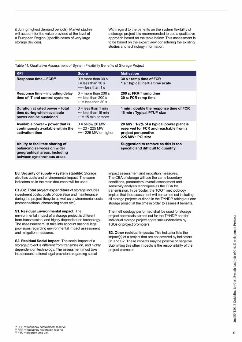
2nd
EN
TSO
-E G
uide
line
for C
ost B
enefi
t Ana
lysi
s of
Gri
d D
evel
opm
ent P
roje
cts
47
34 FCR = frequency containment reserve35 FRR = frequency restoration reserve36 PTU = program time unit
it during highest demand periods). Market studies will account for the value provided at the level of a European Region (specific cases of very large storage devices).
With regard to the benefits on the system flexibility of a storage project it is recommended to use a qualitative approach based on the table below. This assessment is to be based on the expert view considering the existing studies and technology information.
B8. Security of supply – system stability: Storage also has costs and environmental impact. The same indicators as in the main document will be used.
C1./C2. Total project expenditure of storage includes investment costs, costs of operation and maintenance during the project lifecycle as well as environmental costs (compensations, dismantling costs etc.).
S1. Residual Environmental impact: The environmental impact of a storage project is different from transmission, and highly dependent on technology. The assessment must take into account national legal provisions regarding environmental impact assessment and mitigation measures.
S2. Residual Social impact: The social impact of a storage project is different from transmission, and highly dependent on technology. The assessment must take into account national legal provisions regarding social
impact assessment and mitigation measures. The CBA of storage will use the same boundary conditions, parameters, overall assessment and sensitivity analysis techniques as the CBA for transmission. In particular, the TOOT methodology implies that the assessment will be carried out including all storage projects outlined in the TYNDP, taking out one storage project at the time in order to assess it benefits.
The methodology performed shall be used for storage project appraisals carried out for the TYNDP and for individual storage project appraisals undertaken by TSOs or project promoters.
S3. Other residual impacts: This indicator lists the impact(s) of a project that are not covered by indicators S1 and S2. These impacts may be positive or negative. Submitting this other impacts is the responsibility of the project promoter.
Table 11: Qualitative Assessment of System Flexibility Benefits of Storage Project
KPI Score Motivation
Response time – FCR34 0 = more than 30 s += less than 30 s ++= less than 1 s
30 s : ramp time of FCR 1 s : typical inertia time scale
Response time – including delay time of IT and control systems
0 = more than 200 s += less than 200 s ++= less than 30 s
200 s: FRR35 ramp time 30 s: FCR ramp time
Duration at rated power – total time during which available power can be sustained
0 = less than 1 min += less than 15 min ++= 15 min or more
1 min : double the response time of FCR 15 min : Typical PTU36 size
Available power – power that is continuously available within the activation time
0 = below 20 MW += 20 - 225 MW ++= 225 MW or higher
20 MW : 1-2% of a typical power plant is reserved for FCR and reachable from a project perspective 225 MW : PCI size
Ability to facilitate sharing of balancing services on wider geographical areas, including between synchronous areas
Suggestion to remove as this is too specific and difficult to quantify

48
Section 5
Annexes
2nd
EN
TSO
-E G
uide
line
for C
ost B
enefi
t Ana
lysi
s of
Gri
d D
evel
opm
ent P
roje
cts
48

2nd
EN
TSO
-E G
uide
line
for C
ost B
enefi
t Ana
lysi
s of
Gri
d D
evel
opm
ent P
roje
cts
49
2nd
EN
TSO
-E G
uide
line
for C
ost B
enefi
t Ana
lysi
s of
Gri
d D
evel
opm
ent P
roje
cts
49

2nd
EN
TSO
-E G
uide
line
for C
ost B
enefi
t Ana
lysi
s of
Gri
d D
evel
opm
ent P
roje
cts
50
This annex is a transparent information on the practices or guidelines that are followed by TSOs when planning their networks. The information is supported by all TSOs and as such gives an overview of European TSOs best practices. Of course, the presented technical information cannot enter into extended details (such as probabilities or thresholds) because those details will most probably differ, in more or less extent, in all TSOs. The CBA assessment is not a primary planning tool but rather a common methodology which allows to consistently comparing projects which have been previously planned
according to an agreed set of guidelines/best practices. Nonetheless, the CBA methodology builds on the same principles that are used for planning when trying to measure the technical performance of projects.
Technical criteria and methods are required when assessing the planning scenarios, in order to identify future problems and determine the required development of the transmission grid. These assessments take into account the outcomes from the scenarios analysis.
5.1
Annex 1: Technical criteria for planning
5.1.1 Definitions37
D.1. Base Case for grid analysis. Data used for analysis are mainly determined by the planning cases. For any relevant point in time, the expected state of the whole system, “with all network equipment available”, forms the basis for the analysis (“Base case analysis”).
D.2. Contingencies. A contingency is the loss of one or several elements of the transmission grid. A differentiation is made between ordinary, exceptional and out-of-range contingencies. The wide range of climatic conditions and the size and strength of different networks within ENTSO-E mean that the frequency and consequences of contingencies vary among TSOs. As a result, the definitions of ordinary and exceptional contingencies can differ between TSOs. The standard allows for some variation in the categorisation of contingencies, based on their likelihood and impact within a specific TSO network.
— An ordinary contingency is the (not unusual) loss of one of the following elements:
— Generator. — Transmission circuit (overhead, underground
or mixed). — A single transmission transformer or two
transformers connected to the same bay. — Shunt device (i.e. capacitors, reactors, etc.). — Single DC circuit. — Network equipment for load flow control
(phase shifter, FACTS …).
— A line with two or more circuits on the same towers if a TSO considers this appropriate and includes this contingency in its normal system planning.
— An exceptional contingency is the (unusual) loss of one of the following elements:
— A line with two or more circuits on the same towers if a TSO considers this appropriate and does not include this contingency in its normal system planning.
— A single bus-bar. — A common mode failure with the loss
of more than one generating unit or plant. — A common mode failure with the loss
of more than one DC link.— An out-of-range contingency includes the
(very unusual) loss of one of the following: — Two lines independently and simultaneously. — A total substation with more than one bus-bar. — Loss of more than one generation unit
independently.
D.3. N-1 criterion for grid planning. The N-1 security criterion is satisfied if the grid is within acceptable limits for expected supply and demand situations as defined by the planning cases, following a temporary (or permanent) outage of one of the elements of the ordinary contingency list (see D2 and chapter 5.1.2.2).
37 For all definitions, see also ENTSO-E’s draft Operational Security Network Code (https://www.entsoe.eu/resources/network-codes/operational-security/).

2nd
EN
TSO
-E G
uide
line
for C
ost B
enefi
t Ana
lysi
s of
Gri
d D
evel
opm
ent P
roje
cts
51
5.1.2 Common criteria
5.1.2.1 Studies to be performed
C.1. Load flow analysis— Examination of ordinary contingencies. N-1
criterion is systematically assessed taking into account each single ordinary contingency of one of the elements mentioned above.
— Examination of exceptional contingencies. Exceptional contingencies are assessed in order to prevent serious interruption of supply within a wide-spread area. This kind of assessment is done for specific cases based on the probability of occurrence and/or based on the severity of the consequences.
— Examination of out-of-range contingencies. Out-of-range contingencies are very rarely assessed at the planning stage. Their consequences are minimised through Defence Plans.
C.2. Short circuit analysis. Maximum and minimum symmetrical and single-phase short-circuit currents are evaluated according to the IEC 60 909, in every bus of the transmission grid.
C.3. Voltage collapse. Analysis of cases with a further demand increase by a certain percentage above the peak demand value is undertaken. The resulting voltage profile, reactive power reserves, and transformer tap positions are calculated.
C.4. Stability analysis. Transient simulations and other detailed analysis oriented to identifying possible instability shall be performed only in cases where problems with stability can be expected, based on TSO knowledge.
2nd
EN
TSO
-E G
uide
line
for C
ost B
enefi
t Ana
lysi
s of
Gri
d D
evel
opm
ent P
roje
cts
52
5.1.2.3 Best practice
5.1.2.2 Criteria for assessing consequences
R1. Load flow analysis. Failures combined with maintenance. Certain combinations of possible failures and non-availabilities of transmission elements may be considered in some occasions. Maintenance related non-availability of one element combined with a failure of another one may be assessed. Such investigations are done by the TSO based on the probability of occurrence and/or based on the severity of the consequences, and are of particular relevance for network equipment that may be unavailable for a considerable period of time due to a failure, maintenance, overhaul (for instance cables or transformers) or during major constructions.
R2. Steady state analysis. Acceptable consequences depend on the type of event that is assessed. In the case of exceptional contingencies, acceptable consequences can be defined regarding the scale of the incident, and include loss of demand. Angular differences should be assessed to ensure that circuit breakers can re-close without imposing unacceptable step changes on local generators.
R3. Voltage Collapse analysis: The aim of voltage collapse analysis is to give some confidence that there is sufficient margin to the point of system collapse in the analysed case to allow for some uncertainty in future levels of demand and generation.
C.5. Steady state criteria— Cascade tripping. A single contingency must
not result in any cascade tripping that may lead to a serious interruption of supply within a wide-spread area (e.g. further tripping due to system protection schemes after the tripping of the primarily failed element).
— Maximum permissible thermal load. The base case and the case of failure must not result in an excess of the permitted rating of the network equipment. Taking into account duration, short term overload capability can be considered, but only assuming that the overloads can be eliminated by operational countermeasures within the defined time interval, and do not cause a threat to safe operation.
— Maximum and minimum voltage levels. The base case and the case of failure shall not result in a voltage collapse, nor in a permanent shortfall of the minimum voltage level of the transmission grid, which are needed to ensure acceptable voltage levels in the sub-transmission grid. The base case and the case of failure shall not result in an excess of the maximum admissible voltage level of the transmission grids defined by equipment ratings and national regulation, taking into account duration.
C.6. Maximum loss of load or generation should not exceed the active power frequency response available for each synchronous area.
C.7. Short circuit criteria. The rating of equipment shall not be exceeded to be able to withstand both the initial symmetrical and single-phase short-circuit current (e.g. the make rating) when energising on to a fault and the short circuit current at the point of arc extinction (e.g. the break rating). Minimum short-circuit currents must be assessed in particular in bus-bars where a HVDC installation is connected in order to check that it works properly.
C.8. Voltage collapse criteria. The reactive power output of generators and compensation equipment in the area should not exceed their continuous rating, taking into account transformer tap ranges. In addition the generator terminal voltage shall not exceed its admissible range.
C.9. Stability criteria. Taking into account the definitions and classifications of stability phenomena38, the objective of stability analysis is the rotor angle stability, frequency stability and voltage stability in case of ordinary contingencies (see section 5.1..1), i.e. incidents which are specifically foreseen in the planning and operation of the system.
— Transient stability. Any 3-phase short circuits successfully cleared shall not result in the loss of the rotor angle and the disconnection of the generation unit (unless the protection scheme requires the disconnection of a generation unit from the grid).
— Small Disturbance Angle Stability. Possible phase swinging and power oscillations (e.g. triggered by switching operation) in the transmission grid shall not result in poorly damped or even un-damped power oscillations.
— Voltage security. Ordinary contingencies (including loss of reactive power in-feed) must not lead to violation of the admissible voltage range that is specified by the respective TSO (generally 0.95 p.u. – 1.05 p.u).
38 Definition and Classification of Power System Stability, IEEE/CIGRE Joint Task Force, June 2003
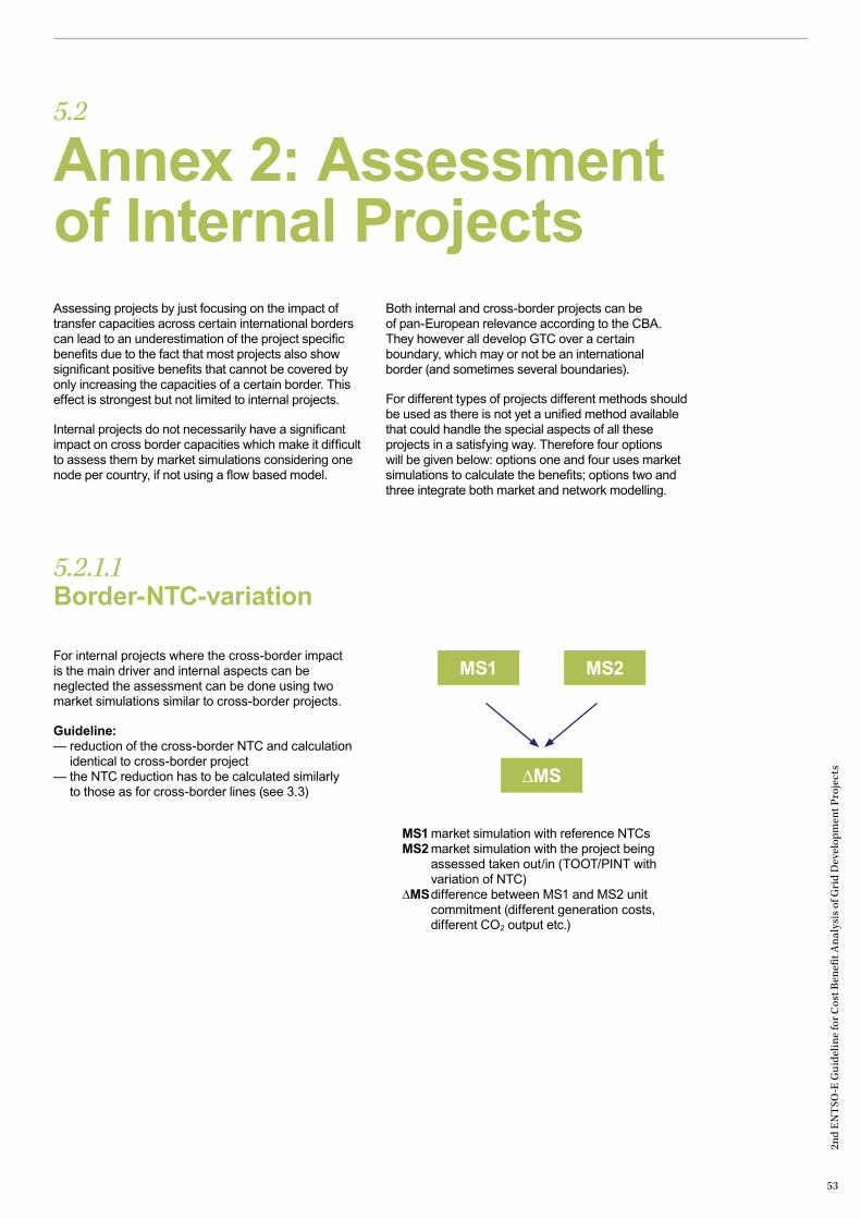
2nd
EN
TSO
-E G
uide
line
for C
ost B
enefi
t Ana
lysi
s of
Gri
d D
evel
opm
ent P
roje
cts
53
5.2.1.1Border-NTC-variation
For internal projects where the cross-border impact is the main driver and internal aspects can be neglected the assessment can be done using two market simulations similar to cross-border projects.
Guideline:— reduction of the cross-border NTC and calculation
identical to cross-border project— the NTC reduction has to be calculated similarly
to those as for cross-border lines (see 3.3)
MS1 market simulation with reference NTCs MS2 market simulation with the project being
assessed taken out/in (TOOT/PINT with variation of NTC)
ΔMS difference between MS1 and MS2 unit commitment (different generation costs, different CO2 output etc.)
Assessing projects by just focusing on the impact of transfer capacities across certain international borders can lead to an underestimation of the project specific benefits due to the fact that most projects also show significant positive benefits that cannot be covered by only increasing the capacities of a certain border. This effect is strongest but not limited to internal projects.
Internal projects do not necessarily have a significant impact on cross border capacities which make it difficult to assess them by market simulations considering one node per country, if not using a flow based model.
Both internal and cross-border projects can be of pan-European relevance according to the CBA. They however all develop GTC over a certain boundary, which may or not be an international border (and sometimes several boundaries).
For different types of projects different methods should be used as there is not yet a unified method available that could handle the special aspects of all these projects in a satisfying way. Therefore four options will be given below: options one and four uses market simulations to calculate the benefits; options two and three integrate both market and network modelling.
5.2
Annex 2: Assessment of Internal Projects
MS1 MS2
ΔMS
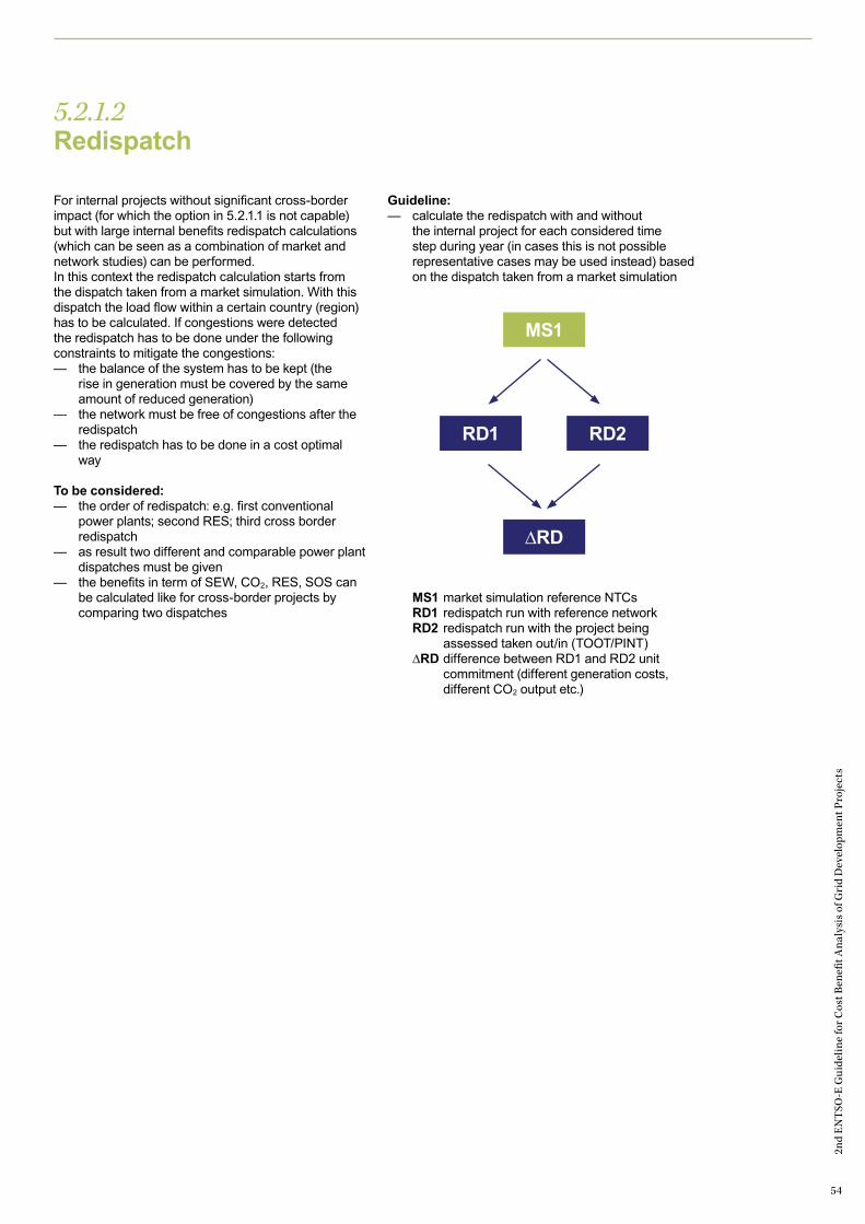
2nd
EN
TSO
-E G
uide
line
for C
ost B
enefi
t Ana
lysi
s of
Gri
d D
evel
opm
ent P
roje
cts
54
5.2.1.2 Redispatch
For internal projects without significant cross-border impact (for which the option in 5.2.1.1 is not capable) but with large internal benefits redispatch calculations (which can be seen as a combination of market and network studies) can be performed. In this context the redispatch calculation starts from the dispatch taken from a market simulation. With this dispatch the load flow within a certain country (region) has to be calculated. If congestions were detected the redispatch has to be done under the following constraints to mitigate the congestions:— the balance of the system has to be kept (the
rise in generation must be covered by the same amount of reduced generation)
— the network must be free of congestions after the redispatch
— the redispatch has to be done in a cost optimal way
To be considered:— the order of redispatch: e.g. first conventional
power plants; second RES; third cross border redispatch
— as result two different and comparable power plant dispatches must be given
— the benefits in term of SEW, CO2, RES, SOS can be calculated like for cross-border projects by comparing two dispatches
Guideline:— calculate the redispatch with and without
the internal project for each considered time step during year (in cases this is not possible representative cases may be used instead) based on the dispatch taken from a market simulation
MS1 market simulation reference NTCs RD1 redispatch run with reference network RD2 redispatch run with the project being
assessed taken out/in (TOOT/PINT) ΔRD difference between RD1 and RD2 unit
commitment (different generation costs, different CO2 output etc.)
RD1 RD2
ΔRD
MS1
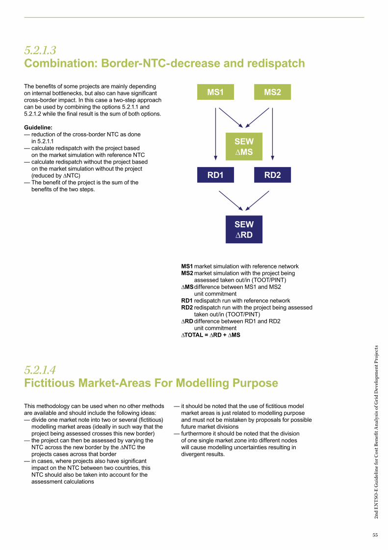
2nd
EN
TSO
-E G
uide
line
for C
ost B
enefi
t Ana
lysi
s of
Gri
d D
evel
opm
ent P
roje
cts
55
5.2.1.3Combination: Border-NTC-decrease and redispatch
5.2.1.4Fictitious Market-Areas For Modelling Purpose
The benefits of some projects are mainly depending on internal bottlenecks, but also can have significant cross-border impact. In this case a two-step approach can be used by combining the options 5.2.1.1 and 5.2.1.2 while the final result is the sum of both options.
Guideline:— reduction of the cross-border NTC as done
in 5.2.1.1— calculate redispatch with the project based
on the market simulation with reference NTC— calculate redispatch without the project based
on the market simulation without the project (reduced by ∆NTC)
— The benefit of the project is the sum of the benefits of the two steps.
This methodology can be used when no other methods are available and should include the following ideas: — divide one market note into two or several (fictitious)
modelling market areas (ideally in such way that the project being assessed crosses this new border)
— the project can then be assessed by varying the NTC across the new border by the ∆NTC the projects cases across that border
— in cases, where projects also have significant impact on the NTC between two countries, this NTC should also be taken into account for the assessment calculations
— it should be noted that the use of fictitious model market areas is just related to modelling purpose and must not be mistaken by proposals for possible future market divisions
— furthermore it should be noted that the division of one single market zone into different nodes will cause modelling uncertainties resulting in divergent results.
MS1 market simulation with reference network MS2 market simulation with the project being
assessed taken out/in (TOOT/PINT) ΔMS difference between MS1 and MS2
unit commitment RD1 redispatch run with reference network RD2 redispatch run with the project being assessed
taken out/in (TOOT/PINT) ΔRD difference between RD1 and RD2
unit commitment ΔTOTAL = ΔRD + ΔMS
MS1
RD1
MS2
RD2
SEWΔMS
SEWΔRD

2nd
EN
TSO
-E G
uide
line
for C
ost B
enefi
t Ana
lysi
s of
Gri
d D
evel
opm
ent P
roje
cts
56
39 In principle the method can also be applied to any kind of boundary.40 Which generators to use for the generation power shift is highly context dependent. As many different methods for the generation power-shift
can be applied without the possibility to identifying a preferable one, no favoured methodology for the generation power-shift is given in this guideline. But it should be mentioned that the generation power-shift can have a significant impact on the results and should therefore be chosen carefully and with a detailed justification. In the likely case where the initial highest N-1 load may be higher or lower that 100%, a power shift relative to the initial dispatch across the boundary is to be applied in order to reach the 100% and find the corresponding power value. Depending on the initial conditions, this power shift would increase or reduce the reference power flow.
This annex delivers an example on how to calculate the ΔNTC using the TOOT approach (PINT approach is similar, only the position of the project towards the reference network model changes); see also Table 11. The following example is designed for a ΔNTC calculation across any boundary between bidding zones39.
Consider the example system as presented in Figure 12 on page 57.
1 Perform load flow analysis on the reference network model in line with the security criteria described in Annex 1, thus taking into account the N-1 criteria
2 Identify the total generation in zone X and Y (in the simple example zone Z does not have any generation or demand) which corresponds with at least one line loaded at exactly 100% under N-1 condition (100% situation) in one of the areas around the border under consideration (i.e. X and Y in the example), and
with no other congestion, under the assumption that there are no congestions in zone Z. The 100%-situation can be created by performing a generation power-shift40 in the zones X and Y (and vice versa).
3 Repeat steps 1 and 2 on the reference network model from which the project has been removed (TOOT of the project for which the ∆NTC shall be determined). This will provide the values for generation in X and Y in the situation when one of the lines is loaded at exactly 100% under N-1 without the project.
4 Calculate the ΔNTC as the difference between the generation situations that correspond with the 100%-situations: ∆NTC equals the power shift.
5 Apply this process to both directions of power flow across the boundary under analysis.
5.3
Annex 3: Example of ΔNTC calculation
Table 12: Simplified example of NTC increase from direction X to Y across a boundary
Example of how to calculate the ∆NTC: Step 1 denotes the initial situation where all projects are put in (including line B). No overloads show up illustrated by the line loadings in %. In Step 2 the generation power-shift has been done until on line is loaded at exact 100% (here line A) under N-1 conditions. The power-shift-volume needed was 500 MW. In Step 3 line B is taken out as per TOOT approach. The dispatch is fixed as it was after Step 2 with +500 MW in zone X and -500 MW in zone Y. The loading of line A became 150% (N-1). In Step 4 the generation power-shift is done in the opposite direction compared to Step 2 to reduce the load on line A to 100% (N-1). The remaining power-shift, compared to the initial situation, is 200 MW. Hence, the project enables a power shift increase of difference between initial dispatch and final dispatch, thus 500 MW – 200 MW = 300 MW. Step 5 illustrates the corresponding ∆NTC in the direction X>Y across the boundary.
Step 1 Step 2 Step 3 Step 4 Step 5
Incident Line B in Line B in TOOT line B TOOT line B ∆ NTC X > Y
[MW] Situation initial situation
100% situation
>100% situation
mitigated situation thus back to 100%
Generation in zone X 400 900 900 600 300
Generation in zone Y 800 300 300 600
demand to be covered 1200 1200 1200 1200
Line loading at line A 80% 100% 150% 100%
Line loading at line B 50% 80% - -

2nd
EN
TSO
-E G
uide
line
for C
ost B
enefi
t Ana
lysi
s of
Gri
d D
evel
opm
ent P
roje
cts
57
Figure 12: Qualitative example to illustrate the single steps as described in the example above. It should be noted that the real physical flow will also have a component across the boundary between the zones X-Z as well as Z-Y.
generation: 400 MW
generation: 800 MW
line B: 50%
line A: 80%
Load
Step 1: Initial situationZone X Zone Z
Zone Y
generation: 900 MW
generation: 300 MW
line B: 80%
line A: 100%
Load
Step 2: 100% situationZone X Zone Z
Zone Y
generation: 900 MW
generation: 300 MW
line B: 50%
line A: 80%
Load
Step 3: >100% situationZone X Zone Z
Zone Y
generation: 600 MW
line A: 150%
line B taken out
generation: 600 MW
line B taken out
line A: 100%
Load
Step 4: Mitigation situationZone X Zone Z
Zone Y

2nd
EN
TSO
-E G
uide
line
for C
ost B
enefi
t Ana
lysi
s of
Gri
d D
evel
opm
ent P
roje
cts
58
ContextThe Regulation (EU) n.347/2013 project requires that this CBA methodology takes into account the impact of transmission infrastructures on market power in Member States. This paper analyses this indicator and its limits, as well as the necessary methodology to construct it.
Basics on methodologyMarket power is the ability to alter prices away from competitive levels. It is important to point out that this ability is a reflection of potential. A market player can have market power without using it. Only when it is actually used, market power has negative consequences on socio-economic welfare, by reducing the overall economic surplus to the benefit of a single market player. Taking into account market power in a CBA therefore requires three steps:— To define carefully which asset(s) will be assessed.
The calculation of the index will be made with and without this object, and the difference on these two calculations will be the outcome of the CBA.
— To define the market on which the index will be applied: geographic extension, how to take into account interconnections and market coupling, treatment of regulated market segments, market products to consider.
— To define a market power index, which require the choosing of an index among existing possibilities such as Residual Supply Index (RSI) or Herfindahl-Hirschman Index (HHI). Each of these has its advantages and disadvantages.
All of these choices affect the results of a market power analysis, i.e. the perceived market power is highly dependent on how it is defined.
Limits of market power indicatorsFirst, it must be highlighted that the calculation of all these indexes requires confidential data as input. Thus, a balance has to be found between the necessary confidentiality of these data and the need for transparency that is required for CBA, as this is a necessary condition to obtain EU permitting and financial assistance.
Furthermore, monetisation of this market power index requires that the impact of a change in the market power index on socio-economic welfare is estimated. This requires that one is able to model the functioning of a future market under the hypothesis of imperfect competition, despite the fact that the validity of such a model is virtually impossible to prove. The inevitable model assumptions can radically change the results. The results of a CBA in terms of market power can therefore only be qualitative, and its use as a reference for cost allocation would raise many objections.
A CBA study is typically performed by evaluating the impact of a project during its whole life cycle. This requires a complete set of hypothesis on the future, for example the evolution of the level of consumption. Unfortunately, market power evolution cannot be modelled, as it is dependent on individual and regulatory decisions. Market structure could change dramatically in the future, for instance as the result of a merger. A solution to this issue could be to assess the impact of the infrastructure on the observed situation only. However, it should be noted that evaluating market power in a different hypothesis framework from the other aspects of the CBA would imply that the results are not consistent, and should not be compared.
Building projects may have a positive impact on market power issues, but it is not the only solution.
The instability of market power compared to the other aspects of a CBA has a crucial impact on its relevance as part of a decision making process. Dealing with generator ownership structures 10 or 20 years from now adds a highly uncertain dimension to the evaluation of European benefits of a given asset. Taking the impact of infrastructure capacity on market power into account in a CBA can heavily affect the identification of priority projects. Moreover, a change in the market structure can completely change the decision of building a particular project. This is all the more important considering that there are other, faster ways to solve market power issues, through regulation for example. By the time a project is completed, it is very likely that the market power issue has already been tackled by the regulator, and the project will not bring any benefit on this aspect. Taking market power into account in a CBA can thus lead to sub-optimal decisions.
ConclusionThe impact of future assets on current market power (which is generally positive) is an important indication, but this short-term aspect cannot be used in the assessment of an investment decision which is, by definition, a long-term commitment. National markets have already begun to merge, through market coupling, and a reporting of benefits on market power by Member States is already outdated.
5.4
Annex 4: Impact on market power
2nd
EN
TSO
-E G
uide
line
for C
ost B
enefi
t Ana
lysi
s of
Gri
d D
evel
opm
ent P
roje
cts
59
Goals of any project assessment method— Transparency: the assessment method must provide
transparency in its main assumptions, parameters and values;
— Completeness: all relevant indicators (reflecting EU energy policy, as outlined by the criteria specified in annexes IV and V of the draft Regulation) should be included in the assessment framework;
— Credibility/opposability: if a criterion is weighted, the unit value must stem from an external and credible source (international or European reference);
— Coherence: if a criterion is weighted, the unit value must be coherent within the area under consideration (Europe or Region-al Group).
The limits of a fully monetised cost benefit analysisA fully monetised CBA cannot cover all criteria specified in Annexes IV and V of the Regulation (EU) No 347/2013, since some of these are difficult to monetise.— This is the case for High Impact Low Probability
events such as « disaster and climate resilience » (multiplying low probabilities and very high consequences have little meaning);
— Other benefits, such as, operational flexibility, have no opposable monetary value today (they qualify robustness and flexibility rather than a quantifiable economic value);
— Some benefits have opposable values at a national level, but no common value exists in Europe. This is the case with, for instance, the Value of Lost Load (VOLL), which depends on the structure of consumption in each country (tertiary sector versus industry, importance of electricity in the economy etc.);
— Some benefits (e.g. CO2) are already internalised (e.g. in socio-economic welfare). Displaying a value in tons provides additional information and prevents double accounting.
As stated in the EC Guide to Cost-Benefit Analysis of Investment Projects, Economic appraisal tool for Cohesion Policy 2014-2020 (2014): “In contrast to CBA, which focuses on a unique criterion (the maximisation of socio-economic welfare), multi-criteria analysis is a tool for dealing with a set of different objectives that cannot be aggregated through shadow prices and welfare weights, as in standard CBA”.
This is why ENTSO-E favours a combined multi-criteria and cost benefit analysis that is well adapted to the proposed governance and allows an evaluation based on the most robust indicators, including monetary values if an opposable and coherent unit value exists on a European-wide level. This approach allows for a homogenous assessment of projects on all criteria.
5.5
Annex 5: Multi-criteria analysis and cost benefit analysis

2nd
EN
TSO
-E G
uide
line
for C
ost B
enefi
t Ana
lysi
s of
Gri
d D
evel
opm
ent P
roje
cts
60
A project with a GTC variation between two bidding areas with a price difference will allow generators in the low price bidding area to supply load in the high price
bidding area. In a perfect market, the market price is determined at the intersection of the demand and supply curves.
5.6
Annex 6: Total surplus analysis
Figure 13: Example of an export region (left) and an import region (right) with no (or congested) interconnection capacity (elastic demand)
Figure 14: Example of an export region and an import region, with a new project increasing the GTC between the two regions (elastic demand)
Demand (R1)
Supply (R1)
ConsumerSurplus(R1)
ProducerSurplus(R1)
Demand (R2)
Supply (R2)
ConsumerSurplus(R2)
ProducerSurplus(R2)
P1
P2
Q (MW)
Export Region (R1)
Q (MW)
Import Region (R2)
Pric
e
Pric
e
Supply (R1)
ConsumerSurplus(R1)
ProducerSurplus(R1)
Supply (R
2)
ConsumerSurplus(R2)
ProducerSurplus(R2)
P1P1’
Q1’Q1 Q2Q2’
P2
P2’
Dem
and (R1)
Dem
and (R2)
Pric
e
Q (MW)
∆Q
Export Region (R1)
Pric
e
Q (MW)
Import Region (R2)
∆Q

2nd
EN
TSO
-E G
uide
line
for C
ost B
enefi
t Ana
lysi
s of
Gri
d D
evel
opm
ent P
roje
cts
61
A new project will change the price of both bidding areas. This will lead to a change in consumer and producer surplus in both the export and import area. Furthermore, the TSO revenues will reflect the change in total congestion rents on all links between the export and import areas. The benefit of the project can be measured through the change in socio-economic welfare. The change in welfare is calculated by:
Change in welfare = change in consumer surplus + change in producer surplus + change in total congestion rents
The total benefit for the horizon is calculated by summing the benefit for all time steps considered in that year.
Inelasticity of demandIn the case of the electricity market, short-term demand can be considered as inelastic, since customers do not respond directly to real-time market prices (no willingness-to-pay-value is available). The change in consumer surplus41 can be calculated as follows:
For inelastic demand: change in consumer surplus = change in prices multiplied by demand
Figure 15: Change in consumer surplus
41 When demand is considered as inelastic, the consumer surplus cannot be calculated in an absolute way (it is infinite). However, the variation in consumer surplus as a result of the new project can be calculated nonetheless. It equals the sum for every hour of the year of :(marginal cost of the area x total consumption of the area) with the project – marginal cost of the area x total consumption of the area) without the project
De
ma
nd
(R
1)
Supply (R1)
ConsumerSurplus(R1)
ProducerSurplus(R1)
Supply (R
2)
ConsumerSurplus(R2)
ProducerSurplus(R2)
P1P1’
Q1’Q1
P2
P2’
Q2Q2’
Pric
e
Q (MW)
∆Q
Export Region (R1)P
rice
Q (MW)
Import Region (R2)
∆Q
Decrease in Consumer Surplus
Increase in Consumer Surplus
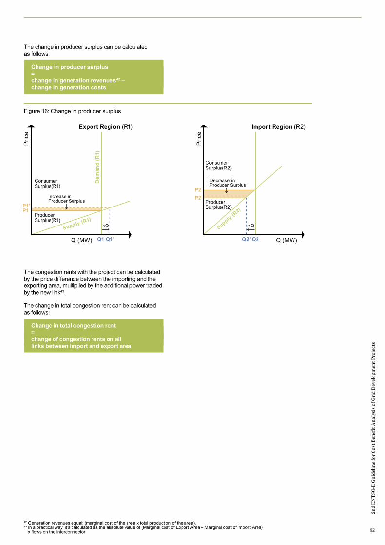
2nd
EN
TSO
-E G
uide
line
for C
ost B
enefi
t Ana
lysi
s of
Gri
d D
evel
opm
ent P
roje
cts
62
The change in producer surplus can be calculated as follows:
Change in producer surplus = change in generation revenues42 – change in generation costs
The congestion rents with the project can be calculated by the price difference between the importing and the exporting area, multiplied by the additional power traded by the new link43.
The change in total congestion rent can be calculated as follows:
Change in total congestion rent = change of congestion rents on all links between import and export area
Figure 16: Change in producer surplus
42 Generation revenues equal: (marginal cost of the area x total production of the area).43 In a practical way, it’s calculated as the absolute value of (Marginal cost of Export Area – Marginal cost of Import Area)
x flows on the interconnector
De
ma
nd
(R
1)
Supply (R1)
ConsumerSurplus(R1)
ProducerSurplus(R1)
Supply (R
2)
ConsumerSurplus(R2)
ProducerSurplus(R2)
P1P1’
Q1’Q1
P2
P2’
Q2Q2’
Pric
e
Q (MW)
∆Q
Export Region (R1)
Pric
e
Q (MW)
Import Region (R2)
∆Q
Increase in Producer Surplus
Decrease in Producer Surplus

2nd
EN
TSO
-E G
uide
line
for C
ost B
enefi
t Ana
lysi
s of
Gri
d D
evel
opm
ent P
roje
cts
63
2nd
EN
TSO
-E G
uide
line
for C
ost B
enefi
t Ana
lysi
s of
Gri
d D
evel
opm
ent P
roje
cts
63

2nd
EN
TSO
-E G
uide
line
for C
ost B
enefi
t Ana
lysi
s of
Gri
d D
evel
opm
ent P
roje
cts
64
The Value of Lost Load (VOLL) is a measure of the costs associated with unserved energy (the energy that would have been supplied if there had been no outage) for consumers. It is generally measured in €/kWh. It reflects the mean value of an outage per kWh (long interruptions) or kW (voltage dips, short interruptions), appropriately weighted to yield a composite value for the overall sector or nation considered. It is an externality, since there is presently no market for security of supply.
The value for VOLL that is used during project assessment should reflect the real cost of outages for system users, hence providing an accurate basis for investment decisions. A level of VOLL that is too high would lead to over-investment, a value that is too low would lead to an inadequate security of supply because the cost of measures to prevent an outage are erroneously weighed against the value of preventing the outage. The optimal level should correspond to the consumer’s willingness to pay for security of supply. Considering VOLL in project assessments should lead to striking the right balance between transmission reinforcements (which have a cost, reflected in tariffs) and outage costs. Transmission reinforcements generally contribute to improving the security and quality of the electricity supply, reduce the probability and severity of outages, and thereby reduce costs for consumers.
Accurately calculating a single value for VOLL that is applicable for pan-European project assessments is presently not possible due to the absence of consistently defined values. Experience has demonstrated that estimated values for VOLL vary significantly by geographic factors, differences in the nature of load composition, the type of affected consumers, and the level of dependency on electricity in the geographical area impacted, differences in reliability standards, the time of year and the duration of the outage. Using a general uniform estimation for VOLL would lead to less transparency and inconsistency, and greatly increase uncertainties compared to presenting the physical units. ENTSO-E does not intend to reduce the accuracy or level of information provided by its assessment results through the application of an estimated VOLL.
Table 12 provides an overview of VOLL values that are reported by different studies across Europe, as the result of an effort to monetize the value of lost load. The overview shows widely varying values, ranging from as little as 0.20 €/kWh (Sweden, households) to more than 200 €/kWh (Austria, industry).
The table on page 65 provides an overview of values for VOLL in Europe, with an indication of the methodology used. The methodologies are not always properly documented; hence no direct comparison of values is possible, nor does ENTSO-E endorse any of the values shown on page 65.
5.7
Annex 7: Value of lost load
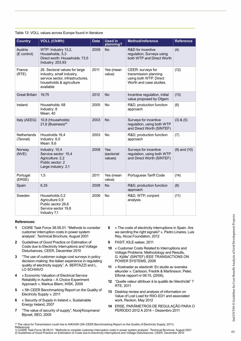
2nd
EN
TSO
-E G
uide
line
for C
ost B
enefi
t Ana
lysi
s of
Gri
d D
evel
opm
ent P
roje
cts
65
References:
1 CIGRE Task Force 38.06.01: “Methods to consider customer interruption costs in power system analysis”. Technical Brochure, August 2001
2 Guidelines of Good Practice on Estimation of Costs due to Electricity Interruptions and Voltage Disturbances, CEER, December 2010
3 “The use of customer outage cost surveys in policy decision-making: the italian experience in regulating quality of electricity supply”, A. BERTAZZI and L. LO SCHIAVO
4 « Economic Valuation of Electrical Service Reliability in Austria – A Choice Experiment Approach », Markus Bliem, IHSK, 2009
5 « 5th CEER Benchmarking Report on the Quality of Electricity Supply », 2011
6 « Security of Supply in Ireland », Sustainable Energy Ireland, 2007
7 “The value of security of supply”, Nooij/Koopmans/Bijvoet, SEO, 2005
8 « The costs of electricity interruptions in Spain. Are we sending the right signals? », Pedro Linares, Luis Rey, Alcoa Foundation, 2012
9 FASIT, KILE-satser, 201110 « Customer Costs Related to Interruptions and
Voltage Problems: Methodology and Results, G. Kjölle” (SINTEF) IEEE TRANSACTIONS ON POWER SYSTEMS, 2008
11 « Kostnader av elavbrott: En studie av svenska elkunder ». Carlsson, Fredrik & Martinsson, Peter, Elforsk rapport nr 06:15, (2006),
12 “Quelle valeur attribuer à la qualité de l’électricité” ? RTE, 2011
13 Desktop review and analysis of information on Value of Lost Load for RIIO-ED1 and associated work, Reckon, May 2012
14 ERSE, PARÂMETROS DE REGULAÇÃO PARA O PERÍODO 2012 A 2014 – Dezembro 2011
Country VOLL (€/kWh) Date Used in planning?
Method/reference Reference
Austria (E control)
WTP: Industry 13,2, Households, 5,3 Direct worth: Households: 73,5 Industry: 203,93
2009 No R&D for incentive regulation, Surveys using both WTP and Direct Worth
(4)
France (RTE)
26. Sectoral values for large industry, small industry, service sector, infrastructures, households & agriculture available
2011 Yes (mean value)
CEER: surveys for transmission planning using both WTP, Direct Worth and case studies.
(12)
Great Britain 19,75 2012 No Incentive regulation, initial value proposed by Ofgem
(13)
Ireland Households: 68 Industry: 8 Mean: 40
2005 No R&D, production function approach
(6)
Italy (AEEG) 10,8 (Households) 21,6 (Business)44
2003 No Surveys for incentive regulation, using both WTP and Direct Worth (SINTEF)
(3) & (5)
Netherlands (Tennet)
Housholds 16,4 Industry: 6,0 Mean: 8,6
2003 No R&D, production function approach
(7)
Norway (NVE)
Industry: 10,4 Service sector: 15,4 Agriculture: 2,2 Public sector: 2 Large industry: 2,1
2008 Yes (sectorial values)
Surveys for incentive regulation, using both WTP and Direct Worth (SINTEF)
(9) and (10)
Portugal (ERSE)
1,5 2011 Yes (mean value)
Portuguese Tariff Code (14)
Spain 6,35 2008 No R&D, production function approach
(8)
Sweden Households 0,2 Agriculture 0,9 Public sector 26,6 Service sector 19,8 Industry 7,1
2006 No R&D, WTP, conjoint analysis
(11)
Table 13: VOLL values across Europe found in literature
44 The value for Transmission could rise to 40€/kWh (5th CEER Benchmarking Report on the Quality of Electricity Supply, 2011).References:1) CIGRE Task Force 38.06.01: “Methods to consider customer interruption costs in power system analysis”. Technical Brochure, August 2001 2) Guidelines of Good Practice on Estimation of Costs due to Electricity Interruptions and Voltage Disturbances, CEER, December 2010

2nd
EN
TSO
-E G
uide
line
for C
ost B
enefi
t Ana
lysi
s of
Gri
d D
evel
opm
ent P
roje
cts
66
Providing a reliable figure for VOLL, which reflects the actual societal costs of an outage, is vital for a proper project assessment with a monetized EENS-component. Once EENS is monetized, this is likely to shift the focus during interpretation of results away from the underlying values (i.e., a value in MWh that is different in each hour and in each price zone) because the monetized value is simply included in the summation of all monetized benefits and costs (e.g., to obtain a simple cost-benefit ratio). This is not problematic if an appropriate set of VOLL-values exists, which properly takes into the account the spatial, temporal, and actoral characteristics that are associated with the cost of EENS. However, if the values used for VOLL in different situations are based on disparate calculation methodologies, which is the case under the present state of knowledge regarding economic valuation of outages, the credibility of the otherwise uniform and standardized project assessment results is undermined. ENTSO-E therefore strongly discourages the use of the values reported in the table above for project assessments and considers the availability of a computation methodology that is approved by ACER and the European Commission as a prerequisite for reporting monetized values of EENS.
The CEER has set out European guidelines45 for nationwide studies on estimation of costs due to electricity interruptions and voltage disturbances, recommending that “National Regulatory Authorities should perform nationwide cost-estimation studies regarding electricity interruptions and voltage disturbances”. Applying these guidelines throughout Europe would help establishing correct levels of VOLL, enabling comparable and consistent project assessments all over Europe. However, this is not yet the case, and an investigation program would be a pre-condition for adopting VOLL for consistent TYNDP or PCI assessments.
Note that in the absence of a uniform and standardized methodology to compute values for VOLL, EENS can nonetheless be monetized by stakeholders that make use of CBA results (e.g. the European Commission during the PCI process). The energy figure expressed in MWh, which ENTSO-E provides as the security of supply indicator in the CBA evaluation of each project, allows all interested parties to monetise by using the preferred VOLL available.
45 Guidelines of Good Practice on Estimation of Costs due to Electricity Interruptions and Voltage Disturbances, CEER, December 2010. Other reports have also established such guidelines, such as CIGRE (2001) and EPRI
2nd
EN
TSO
-E G
uide
line
for C
ost B
enefi
t Ana
lysi
s of
Gri
d D
evel
opm
ent P
roje
cts
67
Exchange and sharing of ancillary services, in particular balancing resources, is crucial both to increase RES integration and to enhance the efficient use of available generation capacities. However, today, there is a great diversity of arrangements for ancillary services throughout Europe46. Common rules for cross-border exchanges of such services are foreseen within the future Network Code on Electricity Balancing. In the absence of such a code, any homogenous assessment of the value of transmission for exchange of ancillary services remains difficult. Some principles established by ACER’s Framework Guidelines on Balancing Services provide a possible scope for cost benefit analysis of ancillary services:— Frequency containment reserves47 are shared and
commonly activated in synchronous areas through the reliability margin foreseen for that purpose. These margins may be included in SEW calculations, and could lead to double-counting.
— The Network Code on Electricity Balancing shall set all necessary features to facilitate the development of cross-border exchanges of balancing energy and stipulate that these are made possible on every border, in the limits defined by Network Code on Load Frequency Control and Reserves concerning the procurement of Ancillary Services such as frequency restoration reserves (FRR) and replacement reserves (RR). However, the reservation of cross-border capacity for the purpose of balancing energy, from FRR and RR, is generally forbidden, except for cases where TSOs can demonstrate that such reservation would result in increased overall social welfare.
In general, the increase of cross-border capacities between bidding zones through grid development would therefore only lead to additional value in terms of balancing energy from frequency restoration reserves and replacement reserves during non-congested time steps. Moreover, the value could only be monetised in certain conditions, as described below.
Many transmission projects, especially new interconnectors between or within coordinated markets, can provide the benefit of good reserve, provided only that the sending market has spare reserve capacity being held. The technical capability of an interconnector to deliver reserve, at various timescales should be carefully evaluated, considering both the technical characteristics of the interconnector and the technical definitions of reserve products in the markets. If at least one of the interconnected markets has a market-based approach in balancing services, such that a price of balancing services can be sensibly projected over a forecast horizon, then a question of monetisation of a
balancing services benefit arises. If these conditions are fulfilled, the following guidance could be given:— If the transmission project lies entirely within one
control area, which has a market-based approach in balancing services, then the benefit of that project, in terms of permitting greater access to market of reserve services should be assessed using forecast prices of reserve within the control area. Note that such prices are normally low – it is unusual to have reserve sources significantly limited by transmission, such that differential prices of reserve is released by extra transmission.
— If the transmission project interconnects two control areas, both of which have a market-based approach in balancing services and similar reserve products, then the reserve benefits of that project should be assessed using forecast prices of reserve within each bidding zone. Note the benefits are two-way. For example, if the interconnector is floating at one hour, then it can let reserve from control area A contribute to the requirement to control area B and simultaneously let reserve from control area B contribute to control area A. But of course, if the interconnector is flowing fully from A to B at that hour, then no reserve benefit in control area B can be also claimed. In general, the reserve benefit will be lower than the trading benefit evaluated under SEW (benefit B1).
— If the transmission project interconnects one control area A, which has a market-based approach in balancing services, with a second control area B which does not, or reserve products are very different, then great care should be exercised in attempting to quantify any reserve benefit. Obviously, zero benefit can be claimed for delivery of reserves from control area A into control area B if control area B does not have a marked based approach in balancing services. A Reserve benefit can only be claimed, if it is thought likely to be able to establish the holding of a Reserve service in control area B able to meet the technical requirements of Reserve in control area A. Further, a prudent forecast should be made of the price of holding the reserve in control area B, and this forecast deducted from the forecasted reserve price in control area A. If in doubt, it should be assumed that the price of holding in control area B exceeds the value in control area A, such that zero reserve benefit is claimed.
— Finally, if the transmission project interconnects two control areas which have no market-based approach in balancing services, then obviously, zero benefit can be claimed for delivery of reserves into either market.
5.8
Annex 8: Assessment of ancillary services
46 See for instance ENTSO-E’s survey on Ancillary Services Procurement and Electricity Balancing Market Design https://www.entsoe.euresources/network-codes/electricity-balancing/.
47 Frequency containment reserves are operating reserves necessary for constant containment of frequency deviations (in order to constantly maintain the power balance in the whole synchronously interconnected system. This category typically includes operating reserves with the activation time up to 30 seconds. Operating reserves of this category are usually activated automatically.
2nd
EN
TSO
-E G
uide
line
for C
ost B
enefi
t Ana
lysi
s of
Gri
d D
evel
opm
ent P
roje
cts
68
As stated in chapter 1, the main objective of transmission system planning is to ensure the development of an adequate transmission system which:— Enables safe system operation;— Enables a high level of security of supply;— Contributes to a sustainable energy supply;— Facilitates grid access for all market participants;— Contributes to internal market integration, facilitates
competition, and harmonisation;— Contributes to improving the energy efficiency
of the system.— Enables cross-country transmissions.
The TYNDP highlights the way transmission projects of European Significance contribute to the EU’s overall sustainability goals, such as CO2 reduction or integration of renewable energy sources (RES). On a local level, these projects may also impact other EU sustainability objectives, such as the EU Biodiversity Strategy (COM 2011 244) and landscape protection policies (European Landscape Convention). Moreover, new infrastructure needs to be carefully implemented though appropriate public participation at different stages of the project, taking into account the goals of the Aarhus Convention (1998) and the measures foreseen by the Regulation on Guidelines for trans-European energy infrastructure (EU n° 347-2013).
As a rule, the first measure to deal with the potential negative social and environmental effects of a project is to avoid causing the impact (e.g. through routing decisions) wherever possible. Steps are also taken to minimise impacts through mitigation measures, and in some instances compensatory measures, such as wildlife habitat creation, may be a legal requirement. When project planning is in a sufficiently advanced stage, the cost of such measures can be estimated accurately, and they are incorporated in the total project costs (listed under indicator C1).
Since it is not always possible to (fully) mitigate certain negative effects, the indicators ‘social impact’ and ‘environmental impact’ are used to: — indicate where potential impacts have not yet been
internalized i.e. where additional expenditures may be necessary to avoid, mitigate and/or compensate for impacts, but where these cannot yet be estimated with enough accuracy for the costs to be included in indicator C1.
— indicate the residual social and environmental effects of projects, i.e. effects which may not be fully mitigated in final project design, and cannot be objectively monetised.
Particularly in the early stages of a project, it may not be clear whether certain impacts can and will eventually be mitigated. Such potential impacts are included and labelled as potential impacts. In subsequent iterations of the TYNDP they may either disappear if they are mitigated or compensated for, or lose the status of potential impact (and thus become residual) if it becomes clear that the impact will eventually not be mitigated or compensated for.
When insufficient information is available to indicate the (potential) impacts of a project, this will be made clear in the presentation of project impacts in a manner that ‘no information’ cannot be confused with ‘no impact’.
In its report on Strategic Environmental Assessment for Power Developments, the International Council on Large Electric Systems (CIGRÉ, 2011) provides an extensive overview of factors that are relevant for performing Strategic Environmental Assessment (SEA) on transmission systems. Most indicators in this report were already covered by ENTSO-E’s cost-benefit analysis methodology, either implicitly via the additional cost their mitigation creates for a project, or explicitly in the form of a separate indicator (e.g. CO2 emissions). Three aspects (‘biodiversity’, ‘landscape’, and ‘social integration of infrastructure’), however, could not be quantified objectively and clearly via an indicator or through monetisation. Previously, these were addressed in the TYNDP by an expert assessment of the risk of delays to projects, based on the likelihood of protests and objections to their social and environmental impacts. Particularly for projects that are in an early stage of development, this approach improves assessment transparency as it provides a quantitative basis for the indicator score.
To provide a meaningful yet simple and quantifiable measure for these impacts, the new methodology improves on this indicator by giving an estimate of the number of kilometres of a new overhead line (OHL), underground cable (UGC) or submarine cable (SMC) that might have to be located in an area that is sensitive for its nature or biodiversity (environmental impact), or its landscape or social value (social impact) (for a definition of “sensitive”: see below).
5.9
Annex 9: Residual environmental and social impact
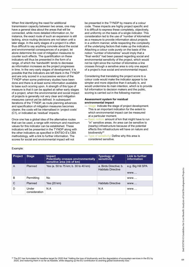
2nd
EN
TSO
-E G
uide
line
for C
ost B
enefi
t Ana
lysi
s of
Gri
d D
evel
opm
ent P
roje
cts
69
When first identifying the need for additional transmission capacity between two areas, one may have a general idea about the areas that will be connected, while more detailed information on, for instance, the exact route of such an expansion is still lacking, since routing decisions are not taken until a later stage. In the early stages of a project it is often thus difficult to say anything concrete about the social and environmental consequences of a project, let alone determine the cost of mitigation measures to counter such effects. The quantification on these indicators will thus be presented in the form of a range, of which the ‘bandwidth’ tends to decrease as information increases as the project progresses in time. In the very early stages of development, it is possible that the indicators are left blank in the TYNDP and are only scored in a successive version of the TYNDP when some preliminary studies have been done and there is at least some information available to base such scoring upon. A strength of this type of measure is that it can be applied at rather early stages of a project, when the environmental and social impact of projects is generally not very clear and mitigation measures cannot yet be defined. In subsequent iterations of the TYNDP, as route planning advances and specification of mitigation measures becomes clearer, the costs will be internalised in ‘project costs’ (C1), or indicated as ‘residual’ impacts.
Once one has a global idea of the alternative routes that can be used, a range with minimum and maximum values for this indicator can be established. These indicators will be presented in the TYNDP along with the other indicators as specified in ENTSO-E’s CBA methodology, with a link to further information. The scores for social and environmental impact will not
be presented in the TYNDP by means of a colour code. These impacts are highly project specific and it is difficult to express these completely, objectively, and uniformly on the basis of a single indicator. This consideration led to the use of “number of kilometres” as a measure to provide information about projects in a uniform manner, while respecting the complexity of the underlying factors that make up the indicators. Attaching a colour code purely on the basis of the notion “number of kilometres” would imply that a “final verdict” had been passed regarding social and environmental sensitivity of the project, which would not be right since the number of kilometres a line crosses through a sensitive area is only one aspect of a project’s true social and environmental impact.
Considering that translating the project score to a colour code would make the indicator appear to be simpler and more objective than it actually is, and would undermine its main intention, which is to provide full information to decision makers and the public, scoring is carried out in the following manner:
Assessment system for residual environmental impact— Stage: Indicate the stage of project development.
This is an important indication for the extent to which environmental impact can be measured at a particular moment.
— Basic notion: amount of km that might have to run “in” sensitive areas. An area can be sensitive to (nearby) infrastructure because of the potential effects this infrastructure will have on nature and biodiversity48
— Type of sensitivity: Define why this area is considered sensitive.
Project Stage ImpactPotentially crosses environmentally sensitive area (nb of km)
Typology of sensitivity
Link to further information
A Planned Yes (a. 50 to 75 km; b. 30 to 40 km) a. Birds Directive; b. Habitats Directive
e.g. Big Hill SPA
www….
B Permitting No www….
C Planned Yes (20 km) Habitats Directive www….
D Under consideration
N.A N.A www….
Example:
48 The EC has formulated its headline target for 2020 that “Halting the loss of biodiversity and the degradation of ecosystem services in the EU by 2020, and restoring them in so far as feasible, while stepping up the EU contribution to averting global biodiversity loss.”

2nd
EN
TSO
-E G
uide
line
for C
ost B
enefi
t Ana
lysi
s of
Gri
d D
evel
opm
ent P
roje
cts
70
Assessment system for residual social impact— Stage: Indicate the stage of project development.
This is an important indication for the extent to which social impact can be measured at a particular moment.
— Basic notion: # of km “in” sensitive area. An area can be sensitive to (nearby) infrastructure if it is densely populated or protected for its landscape value.
— Type of sensitivity: Define why this area is considered sensitive.
Definitions:This section provides an overview of impacts that may qualify an area as environmentally or socially ‘sensitive’.
Environmental impact— Sensitivity regarding biodiversity: — Land protected under the following Directives or
International Laws: — Habitats Directive (92/43/EEC) — Birds Directive (2009/147/EC) — RAMSAR site — IUCN key biodiversity areas — Marin Strategy Framework Directive
(2008/56/EC) — Other nature protection areas under
national law
Social impact— Sensitivity regarding population density: — Land that is close to densely populated areas
(as defined by national legislation). As a general guidance, a dense area should an area where population density is superior to the national mean.
— Land that is near to schools, day-care centres, or similar facilities
— Sensitivity regarding landscape: protected under the following Directives or International Laws:
— World heritage — Land within national parks and areas
of outstanding natural beauty — Land with cultural significance — Other areas protected by national law
Project Stage ImpactCrosses dense area (nb of km)
SensitivityTypology of sensitivity
Link to further information
A Permitting Yes (20 to 40km) Dense area www….
A Planned Yes (100 km) European Landscape Convention:
www….
B Planned No Submarine cable www….
C Under construction Yes (50 km) Dense area, OHL www….
Example:

2nd
EN
TSO
-E G
uide
line
for C
ost B
enefi
t Ana
lysi
s of
Gri
d D
evel
opm
ent P
roje
cts
71
2nd
EN
TSO
-E G
uide
line
for C
ost B
enefi
t Ana
lysi
s of
Gri
d D
evel
opm
ent P
roje
cts
71

2nd
EN
TSO
-E G
uide
line
for C
ost B
enefi
t Ana
lysi
s of
Gri
d D
evel
opm
ent P
roje
cts
72
End note.System development tools are continuingly evolving, and it is the intention that this document will be reviewed periodically pursuant to Regulation (EU)
n.347/2013, Art.11 §6, and in line with prudent planning practice and further editions of the TYNDP document of ENTSO-E.

2nd
EN
TSO
-E G
uide
line
for C
ost B
enefi
t Ana
lysi
s of
Gri
d D
evel
opm
ent P
roje
cts
73

2nd
EN
TSO
-E G
uide
line
for C
ost B
enefi
t Ana
lysi
s of
Gri
d D
evel
opm
ent P
roje
cts
74
ENTSO-E AISBL Avenue de Cortenbergh 100, 1000 Brussels, Belgium
Tel (+32) 2 741 09 50
[email protected] www.entsoe.eu
©ENTSO-E 2018
Related Documents