2DS01 Statistics 2 for Chemical Engineering lecture 4.

2DS01

Statistics 2 for Chemical Engineering

lecture 4

2

Contents• Summary of previous lectures• Limitations of factorial designs and standard

RSM designs• mixture designs• D-optimal designs

3

Summary of previous lectures

• one-way ANOVA: compare means of several groups

• noise reduction through blocking• factorial designs:

– screening•blocks• fractions•centre points

– optimisation•steepest ascent•designs

– CCD– Box-Behnken

4

• factors:– amount of adhesive– temperature

• constraints (in terms of coded variables)– too little adhesive at too low temperature:

unsatisfactory bonding– too much adhesive at too high temperature: damage

• experimental region:

Example 1: adhesive

5

Example 2: separation of chlorophenols• Factors:

– pH– percentage organic modifier

• Constraints:– retention times should be not too short nor too long

• Model (based on RPLC knowledge): – complete second order model + 3rd order term in pH

• Experimental region:

6

Example 3: Blending of gasoline• Factors:

– types of octanes• Constraints:

– effect of octanes only depends on proportions

• Model– not known in general; sometimes only small

number of octanes are active• Experimental region:

– simplex (triangle, tetrahedron)

7

Mixtures: necessity for new designs• for independent factors, factorial designs are

suitable (exp. region: hypercube)• in mixtures, factors are dependent because

they add up to 100%• notions of effects and interactions do not carry

over to mixture experiments• hypercube experimental regions give poor

coverage of experimental region of mixtures:

8

Mixture designs• factors are ingredients of mixture• factors are dependent• constraints:

– 0 xi 1

– x1 + x2 + x3 +... + xp = 1

• experimental region is simplex:

x1 + x2 = 1 x1 + x2 + x3= 1

9

Trilinear coordinate system

x2

x1

x3

0.8

0.6

0.4

0.2

(1,0,0)

(0,1,0)

(1/2, 1/2,0)

(0,0,1)

(1/3,1/3,1/3)

10

• {p,m} -simplex lattice design – p = number of factors– m+1 = number of factor levels

• xi = 0, 1/m, 2/m, ..., 1 (i = 1, ..., p)• total number of design points:

Examples:

Simplex lattice design

1p m

m

{3,2} lattice

{3,3} lattice

11

• p components:

– p permutations of (1,0,...,0)

– permutations of (1/2,1/2,0,....,0)

– permutations of (1/3,1/3,1/3,0,....,0)

– ....

– total 2p-1 design points

Example: 3 components

Simplex centroid design

2

p

3

p

x1 = x2 = x3= 1/3

x1 = x2 = 1/2

x2 = x3 = 1/2

x2 = x23 = 1/2

x2 = 1

x1 = 1

x3 = 1

12

Models for mixture designsPolynomial models for mixture responses may be written in different ways because of constraint x1+ x2 + x3 +... + xp = 1.

Usual interpretation of constant term does not make sense (measurements at (0,0,...,0) are impossible). The constant term can always be removed, e.g., for 3 components we may write

( )

0 1 1 2 2 3 3

0 1 2 3 1 1 2 2 3 3

0 1 1 0 2 2 0 3 3( ) ( ) ( )

x x x

x x x x x x

x x x

b b b b

b b b b

b b b b b b

+ + + =

+ + + + + =

+ + + + +

13

Scheffé canonical polynomialsIn order to have meaningful interpretations of coefficients, one applies canonical forms of polynomials for mixture data. Scheffé introduced the following polynomials (examples for p=3):

• linear:

• quadratic

• special cubic

• cubic

There exist other types of canonical polynomials:• Cox polynomials• homogeneous polynomials (Kronecker type)

1 1 2 2 3 3x x xb b b+ +

1 1 2 2 3 3 12 1 2 13 1 3 23 2 3x x x x x x x x xb b b b b b+ + + + +

1 1 2 2 3 3 12 1 2 13 1 3 23 2 3 123 1 2 3x x x x x x x x x x x xb b b b b b b+ + + + + +

1 1 2 2 3 3 12 1 2 13 1 3 23 2 3

12 1 2 1 2 13 1 3 1 3 23 2 3 2 3 123 1 2 3( ) ( ) ( )

x x x x x x x x x

x x x x x x x x x x x x x x x

b b b b b b

g g g b

+ + + + + +

- + - + - +

14

Mixture models: interpretation of coefficients

usual interpretation of interaction no longer holds due to dependence mixture factors

• i is expected response when xi =1 and xj =0 (“pure blend”)• i + j + ij is expected response when xi +xj =1 • excess ij indicates “interaction” effect:

- ij > 0: “(binary) synergistic blending” - ij < 0: “(binary) antagonistic blending”

1 1 2 2 3 3 12 1 2 13 1 3 23 2 3x x x x x x x x xb b b b b b+ + + + +

15

Simplex-lattice versus simplex centroid designs

• simplex-lattice allows for fine grid on experimental region

• {p,m} simplex-lattice cannot detect synergisms of order higher than m

• simplex centroid may be executed sequentially (first pure blends, then binary mixtures, ...)

• both designs have most of their points on the boundary ( = at least one factor equal to 0 )

16

General recommendations for mixture designs

• allow enough degrees of freedom (# design points - # model terms) to allow precise estimation of variance – add extra points of special interest– replicate design

• add points in interior – to increase coverage of experimental region– to increase degrees of freedom for variance

estimation• perform lack-of-fit test if there are replicates • use linear model when screening; use higher-order

models for optimization• perform blocking if necessary

17

Various remarks about mixture designs• mixture designs may be combined with

factorial designs when some variables are not related to the mixture (“process variables”)

• pseudocomponents may be used when there are further restrictions on the mixture ingredients like 0 ≤ xi ≤ 0.3

18

Example of analysis of mixture data• octane blending with 3 components• response is octane rating• goal is optimization of octane rating• simplex centroid design

– 23-1 = 7 points– two additional check points of commercial interest

of current production process– every observation repeated, so in total 18

observations – all experiments under same conditions, so no

blocks• because the goal is optimization, we start with the

quadratic model (simplest model that allow optimization)

19

Results of analysis mixture data: quadratic model

• residuals look OK• significant model (p-value in ANOVA < 0.05; see also high R2)• BUT: significant lack-of-fit (option must be actived in

Statgraphics by using right-mouse click)

ANOVA for octane

--------------------------------------------------------------------------------

Source Sum of Squares Df Mean Square F-Ratio P-Value

--------------------------------------------------------------------------------

Quadratic Model 372.401 5 74.4802 629.41 0.0000

Lack-of-fit 1.90993 3 0.636644 5.38 0.0214

Pure error 1.065 9 0.118333

--------------------------------------------------------------------------------

Total (corr.) 375.376 17

R-squared = 99.2075 percent

R-squared (adjusted for d.f.) = 98.8773 percent

Standard Error of Est. = 0.343996

20

Results of analysis mixture data: special-cubic model

• choose next simplest model (leaves more degrees of freedom for accurate estimation of error variance)

• residuals look OK• significant model (p-value in ANOVA < 0.05) and no

significant lack-of-fitANOVA for octane

--------------------------------------------------------------------------------

Source Sum of Squares Df Mean Square F-Ratio P-Value

--------------------------------------------------------------------------------

Special Cubic Model 374.264 6 62.3774 527.13 0.0000

Lack-of-fit 0.0467705 2 0.0233853 0.20 0.8241

Pure error 1.065 9 0.118333

--------------------------------------------------------------------------------

Total (corr.) 375.376 17

R-squared = 99.7038 percent

R-squared (adjusted for d.f.) = 99.5423 percent

Standard Error of Est. = 0.343996

21

Further results special-cubic model• residuals show only light indication of not being normally distributed• slight pattern in residual plots (variance not constant)• BC “ interaction” not significant (unimportant when optimizing)• antagonistic blending of AB and AC

Special Cubic Model Fitting Results for octane

-----------------------------------------------------------------------------

Standard T

Parameter Estimate Error Statistic P-Value

-----------------------------------------------------------------------------

A:X1 100.847 0.224688

B:X2 85.4195 0.22239

C:X3 85.4941 0.224561

AB -16.3327 1.09311 -14.9415 0.0000

AC -10.72 1.09907 -9.75369 0.0000

BC 0.139025 1.08189 0.128502 0.9001

ABC 29.1457 6.7883 4.29352 0.0013

-----------------------------------------------------------------------------

R-squared = 99.7038 percent

R-squared (adjusted for d.f.) = 99.5423 percent

Standard Error of Est. = 0.317915

22

Trace Plot for octaneReference Blend: 0.333333 0.333333 0.333333

0 0.2 0.4 0.6 0.8 1

Pseudo components

85

89

93

97

101

octa

ne

ComponentX1X2X3

Optimization results• optimum near x1=1.0

Contours of Estimated Response Surface

octane84.0-85.585.5-87.087.0-88.588.5-90.090.0-91.591.5-93.093.0-94.594.5-96.096.0-97.597.5-99.099.0-100.5

X1=1.0

X2=1.0 X3=1.0X1=0.0

X2=0.0X3=0.0

23

Limitations of factorial designs + classical RSM designs

• experimental region may not be hypercube– impossibility to reach corner experimental region – specific constraints– process factors are ingredients of mixture

• chemical knowledge postulates asymmetrical model– interaction not possible– extra higher order term for one factor

Factorial designs and classical RSM designs (CCD, Box-Behnken) cannot be used in these circumstances.

24

Some desirable properties of designs

1. require minimum number of experimental runs2. allows precise estimates of regression

coefficients3. allows precise predictions of responses4. allows experiments to be performed in blocks5. make it possible to detect lack-of-fit

Note: 2. and 3. seem similar, but are not the same!

We will generalize the use of corner points in 2p designs using criterion 2.

25

Example: simple linear regression• given: minimal and maximal settings of factor• problem: which settings are optimal for determining

slope?

large effect in slope small effect in slope

min maxmin max

26

Simple linear regression: variance of slope

0 0

20 1

2

0 1,

1

_

^ 1

1 2_

1

2^ ^

1 11 2_

1

, (0, )

measurements ( , ), 1,...,

Least Squares Criterion: min

and

i i

n

i ii

n

i ii

n

ii

n

ii

Y x N

x y i n

y x

y x x

x x

E Var

x x

27

Distribution of design points: simple linear regression

Recall: variance of slope small if large

Experimental region: -1 x +1

n = 2: x1 = -1 and x2 = +1 (or vice-versa): S = 2

n = 3 : • x1 = -1 , x2 = 0, x3 = +1: S = 2• x1 = -1 , x2 = -1, x3 = +1: S = 8/3 > 2• x1 = -1 , x2 = c, x3 = +1: S = 2/3 * (c2+3) • “optimal solution” (not feasible!) :

– 1 ½ measurement at –1– 1 ½ measurement at +1

2_

1

n

ii

S x x

28

General setup: matrix formulation

^ ^1 2 1

1

2

( ) , is vector of responses

is design matrix, is vector of regression coefficients

( ) , Cov ( )

Special case simple linear regression:

1

,

1

t t t

it

i in

E Y X Y

X

X X X Y X X

xn x

X X Xx x

x

222 1

2_

1

( ) t i i

ni

ii

x xX X

x nn x x

29

Design matrix: quadratic linear regression

^ ^1 2 1

20 1 2

22

1 12 3

2 2 3 4

( ) , is vector of responses

is design matrix, is vector of regression coefficients

( ) , Cov ( )

1

,

1

t t t

i i

ti i i

n n i i i

E Y X Y

X

X X X Y X X

Y x x

n x xx x

X X X x x x

x x x x x

30

Information matrix and confidence regions

Confidence region for regression parameters:

21

ˆ ˆ ( )t

t pn pX X ps F

Properties of confidence region:• it is an ellipsoid• volume proportional to (det(XtX)-1)1/2

• length of axes proportional to (eigenvalues)1/2 of (XtX)-1

31

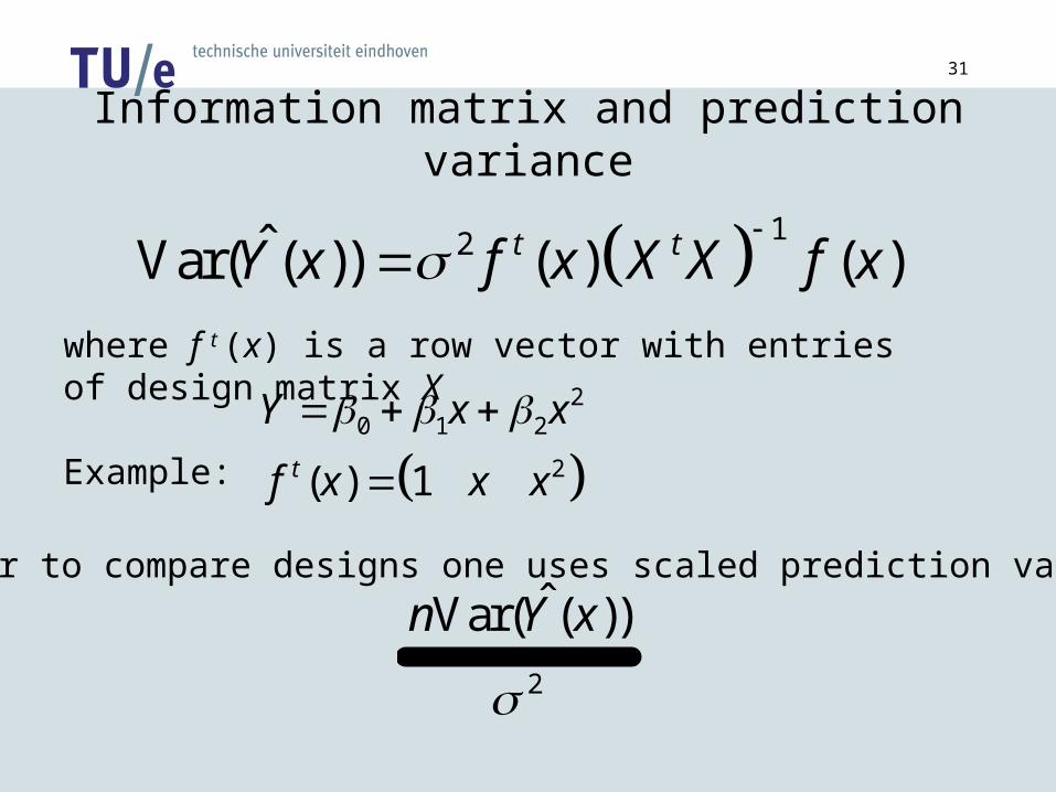
Information matrix and prediction variance

12ˆVar( ( )) ( ) ( )t tY x f x X X f x

where f t (x) is a row vector with entries of design matrix X

Example: 2

0 1 2

2( ) 1t

Y x x

f x x x

In order to compare designs one uses scaled prediction variance:

2

ˆVar( ( ))n Y x

32

Comparison of designs: n=3E(Y) = 0 + 1 x1

– design -1,0,1• (Xt X)-1(2,2)=1/2

•scaled predicted variance: 1 + 3/2 x2

• E(Y) = 0 + 1 x1

– design -1,1,1• (Xt X)-1(2,2)=3/8•scaled predicted

variance: 3/8*(3-2x + 3 x2)

-1 -0.5 0.5 1

0.5

1

1.5

2

2.5

3

-1 -0.5 0.5 1

0.5

1

1.5

2

2.5

3

better choice for maximum predicted variance

better choice for slope

33

Exact design versus continuous designs• mathematical design puts weights on design

points• exact design

– optimal distribution – may not be feasible (non-integer weights)

• continuous design:– optimal distribution with integer weights– is feasible

34

Confidence region: example 11 small variance, i.e. known with high precision

2 large variance, i.e. known with low precision

• axes ellipsoid parallel to coordinate axes, hence parameter estimates for 1 and 2 uncorrelated

2

1

35

Confidence region: example 21 and 2 known with same precision

• axes ellipsoid parallel to coordinate axes, hence parameter estimates for 1 and 2 uncorrelated

2

1

36

Confidence region: example 31 medium variance, i.e. known with medium precision

2 large variance, i.e. known with low precision

• axes ellipsoid not parallel to coordinate axes, hence parameter estimates for 1 and 2 correlated

2

1

37

Optimality criteriaSeveral criteria are being used to construct optimal

designs:• based on ( X t X )-1:

– A-optimality (maximize trace = sum of eigenvalues)– D-optimality (maximize determinant)

• based on prediction variance– G-optimality (minimize maximum scaled prediction

variance)– V-optimality (minimize average scaled prediction

variance)

Note: usual 2p designs are D-optimal!

38

Algorithms•several algorithms exist to compute (approximately) D-optimal designs

•algorithms usually require candidate set of design points

•exhaustive search of all possible subsets often not possible

•exchange algorithms try to optimize criterion by exchanging candidate points or coordinates of candidate points

39

Software• Matlab -> Statistics Toolbox

– cordexch (coordinate exchange algorithm)– rowexch ( row exchange algorithm)– x2fx (generates design matrix for standard

models)

• Statgraphics ->Special -> Experimental Design -> Optimize Design

• Gosset: http://www.research.att.com/~njas/gosset/ (limited Windows version (called Strategy) available at http://www.strategy4doe.com/ )

40

Example: separation of chlorophenols• steps in pH: 0.1• steps in organic modifier: 1%• constraints

– 5.7 pH 7.2– 24% % modifier 50%– modifier+14.8*pH 129.8

• model: Y = 0 + 1 x1 + 2 x2 + 11 x1

2 + 22 x2

2+ 12 x1 x2 + 111 x1

3

• minimal 7 runs necessary for 7 parameters + additional runs to estimate variance

• possible combinations to check????257

7

41

Literature• P.F. de Aguiar et al., D-optimal designs (tutorial),

Chem. Intell. Lab. Syst. 30 (1995), 199-210.• L.E. Eriksson et al., Mixture design – design

generation, PLS analysis, and model usage (tutorial), Chem. Intell. Lab. Syst. 43 (1998), 1-24.

• NIST Engineering Statistics Handbook: http://www.itl.nist.gov/div898/handbook/