2D Resistivity Imaging and Geotechnical Investigation of Structural Collapsed Lecture Theatre in Adekunle Ajasin University, Akungba-Akoko, Southwestern, Nigeria

Aplinkos tyrimai, inžinerija ir vadyba, 2014. Nr. 3(69), P. 49-59 ISSN 1392-1649 (print) Environmental Research, Engineering and Management, 2014. No. 3(69), P. 49-59 ISSN 2029-2139 (online)

http://erem.ktu.lt

49

2D Resistivity Imaging and Geotechnical Investigation of

Structural Collapsed Lecture Theatre in Adekunle Ajasin

University, Akungba-Akoko, Southwestern, Nigeria

Cyril Chibueze Okpoli Department of Geology, Adekunle Ajasin University, Akungba- Akoko, Nigeria

http://dx.doi.org/10.5755/j01.erem.69.3.5335

(Received in September, 2013; accepted in September, 2014)

Geotechnical and geophysical investigation involving electrical resistivity survey and laboratory test of

the samples were conducted on the samples obtained at the three different locations in the area. The study is

aimed at evaluating the competence of the near surface formation building construction materials.

Geophysical and geotechnical methods of investigation were adopted. The Electrical Resistivity Tomography,

using Dipole-Dipole configuration and soil analysis techniques were adopted. A total of four traverses and

three soil samples from different location within the study area were used for the study.

The geophysical results revealed that the topsoil is within the depth of 0 to 5m and it is reflective of

varying resistivity which indicates materials suspected to be composed of low resistive materials such as

water and underlain with a basement complex and presence of a very low resistivity in which water

accumulate and percolate which makes it inimical to foundation of engineering structures. There is an evident

of geological feature such as fracture within the bedrock which might aid subsidence in the area. while

geotechnical results of natural moisture content, specific gravity, liquid limits, plastic limit, plasticity index,

linear shrinkage, compaction and permeability ranges from 5.3-9.2%, 2.620-2.730, 23.0-41.9%, not plastic to

21.4%, from not plastic to 22.4%, 1.4-9.3,1790-2114 kg/m3, 9.1-9.9 and very low to medium respectively.

Thus, the soil formation in the study area is therefore rated as relatively poor for foundation material.

Key words: geotechnical, dipole-dipole, sub-grade, basement complex, engineering structures

1. Introduction

Electrical resistivity tomography and

geotechnical method have been important for

environmental and engineering site delineation, and

routinely applied for structural failures (Dahlin and

Loke, 1998; Olayinka, 1999). The characterization of

engineered structural geology, hydrogeology and

geotectonics have greatly improved in recent times

(Aizebeokhai et.al., 2010, Binley et.al, 2002).

Subsurface instabilities and foundation failures

assessment is now a great concern to engineers and

geoscientists all around the world. A well-constructed

building on a good foundation may fail if subjected to

an extraordinary load, for example, a building

originally designed for residential purpose and

converted to a factory, Mesida, (1987). They live load

which is the sum of the weight of machines,

furniture’s, products and the effect of vibration of

these machines will be greater than the initial live

load before the conversion of the building to factory

(Ranjan and Roa, 2000).

Instances of continuity or preponderance of

mobile structures or structures or structural cracks,

monitoring and repairs of building are routinely

recommended (Donald and Cohen, 1998).

Tomlingson et.al, 1978 classified the extent of wall

cracking ranging from negligible hairline 0.1-1mm to

the very sever cracks (>25mm) which demands

partial, major or complete rebuilding.

Most importantly, the geophysicists, engineering

geologists have placed the cause the foundation

mobility on the competence of the soil which can

support the loads of structures (Sands, 2006). Though

some fractured rocks carry loads, most foundation-

based structural failure are the weak zones of a

Cyril C. Okpoli

50

fracture rocks. In the same vein geological factors are

also important causes of building failure. The

geological structures (or near–surface linear features)

lateral or lithological heterogeneity and incompetence

of sub-surface or surface formation supporting super

structure and thinning out of facies lead to collapse of

building. If a building is found on any of these

geological structures, it may not be able to resist shear

failures. Similarly, construction of a building on a

chemically active rock for example carbonate rocks

(such as limestone and Marble) may cause a building

to fail

Swelling and shrinkage of clays are due to

climatic factors which alters the soil moisture.

Shrinkage of clays leads to subsidence to ground

surface, thus causing a colossal damage of

superstructure. Biological factors like tree planting

and subsequent removal around existing structure

reduce soil water content especially when clays are

removed.

Figure 1 shows a sample of lecture theatre where

2D dipole-dipole and geotechnical survey were

carried at Adekunle Ajasin University, Akungba-

akoko lecture theatre to investigate the geophysical,

geotechnical and engineering characterization of the

subsurface.

Fig. 1. Sample of affected building structure from the area

2. Site description and geology

The study area lies within latitude 70 28 85‘N -

7028 86’N and longitude 005 44 46’E - 005 44 48’ E

in Adekunle Ajasin University, Akungba-akoko.

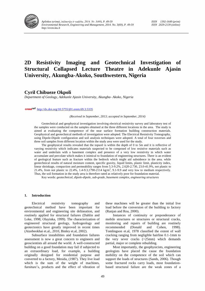
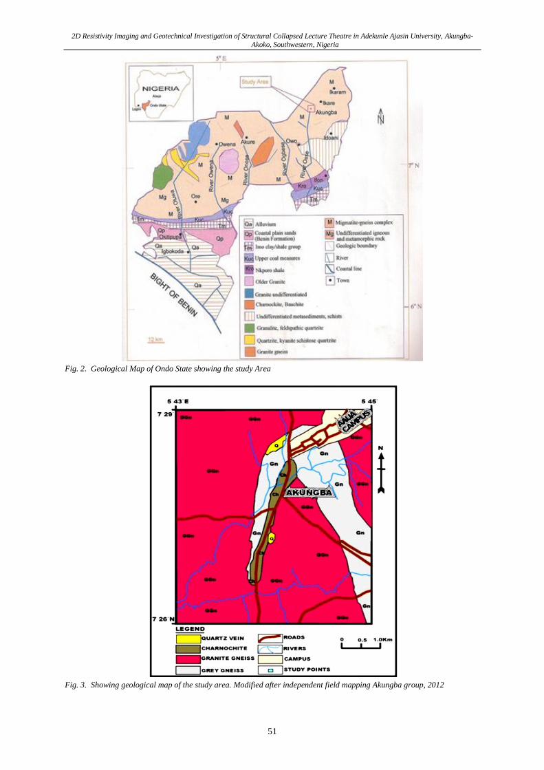
Figure 2 and three show both the geological map of

Ondo state and Akungba-akoko respectively in the

figure below. The study area is characterized by

dendritic drainage pattern. It is observed that some of

the rivers and their tributary streams in the study area

trend east of North while other trend West of North.

These trends are influenced by topography and the

joint system. Its climate is predominantly rainforest

characterized by two seasons-the wet season (between

April-October) and the dry season (between October-

March) with a mean annual rainfall of 1250 mm and a

temperature range of 18 to 33°C. The topography is

generally undulating with Eastward highlands of

granitic origin. The study area lies within the

basement complex of the South-Western Nigeria. The

study area is characterized by Precambrian Basement

rocks such as: grey gneiss, quartzo-feldspathic gneiss,

charnockite; granite gneiss; and porphyritic gneiss

and they are believed to have evolved in at least four

orogenic events namely: the Pan African (600±150

My), The Kibaran (1100±200 My), The Eburnean

(2000±My) and the Liberian (2800±200 My). The

Migmatite- gneiss complex dominate the basement

complex in the study area composed of fairly uniform

biotite and biotite – hornblende-gneiss with locally

intercalated bands of aplitic quartz veins (Ajibade

et.al, 1989).

2D Resistivity Imaging and Geotechnical Investigation of Structural Collapsed Lecture Theatre in Adekunle Ajasin University, Akungba-

Akoko, Southwestern, Nigeria

51

Fig. 2. Geological Map of Ondo State showing the study Area

Fig. 3. Showing geological map of the study area. Modified after independent field mapping Akungba group, 2012

Cyril C. Okpoli

52

3. Material and methods

3.1. 2D Electrical resistivity imaging

The electrical resistivity (dipole-dipole array)

method of geophysical survey was used in S – N and

E-W direction in AAUA campus. Four traverses with

inter- traverse separations of 50 m were mapped out

The ABEM 1000 SAS Terameter Resistivity Meter

was used in acquiring the electrical resistivity data

using the dipole-dipole configuration. The equipment

is capable of measuring apparent resistivity with

induced polarization (IP) or self -potential (SP) at the

same time, though with increase data acquisition time.

The dipole-dipole data were acquired at an electrode

spacing of 5 m on all the traverses with an expansion

factor ‘n’ ranging from 1 – 5 and applying 2-D

inversion software to generate current density sections

and the dipole-dipole pseudosections. The data is

inverted from apparent resistivity through “true”

resistivity by Earth-Imager software “Diprowin

software”. The goal is to create an image of the

ground in terms of electrical resistivity showing both

the lateral and depth extent of area of investigation.

The resistivities of the blocks were iterated and

adjusted until the calculated and field apparent

resistivities agreed to barest minimum differences

(Loke et.al , 2003).

The Pseudo section obtained from DIPROWIN

SOFTWARE using Jacobian iteration is presented

below. The differences of the eight iterations done;

were expressed in percentage as root-mean-square

error (RMS error), which ranges from 5.43 to 7.87 for

the present work.

3.2. Engineering Laboratory Characterization 3.2.1. Index properties (classification) test

Classification tests were carried out on all the

representative soil samples includes; grain size

distribution analysis, wet sieving, drying sieving and

the experimental procedure.

The natural moisture content was performed to

determine the water (moisture) content of soils and is

expressed in percentage. The apparatus are: drying

oven, balance, Moisture can, Gloves, Spatula.

About 100 g of each of the soil sample was

preserved in a cellophene bag immediately after

collection and then transfer to the laboratory to be

weighed in the weighing balance in order to minimize

loss of moisture through evaporation. The weighed

sample was placed in a thermostatically controlled

oven at a constant temperature of 105 0C for 24 hours.

This was removed and allowed to cool. It is necessary

for the dried soil sample to cool before weighing to

accuracy of 0.1 because the hot container can impair

the sensitivity of the balance by irregular expansion.

The natural moisture content of the soil sample

was calculated using the formula:

Mc =𝑊2−𝑊3

(𝑊3−𝑊1)x100 (1)

Where: W1 - Weight of empty container, g;

W2 - Weight of container with moist soil, g;

W3 - Weight of container dried soil, g;

Mc - Water moisture content, %.

3.2.2. Grain size analysis

I classified the soil sample by size of the

individual particles. This test is important in order to

determine the percentage of the various grain sizes

contained in the soil.

The stages involved in grain size determination

are:

(a) Sieve analysis (Mechanical) coarse grain soil.

(b) Hydrometer analysis of fine soil.

Coarse-grained soils behave in nature as

individual particles. They are subdivided into gravel

and sand. Gravel soils have particles sizes coarser

(larger) than about the no 4 or no 10 mesh sieve

opening, depending upon which particular

classification system is used. Sand have particle sizes

finer than gravel (no 4 or no 10 mesh) and coarser

than no 200 mesh sieve, Coarser sand particles pass

through the no 4 sieve and are retained on the no 10

mesh sieve. Medium sand has a particle size that is

smaller than the no 10mesh sieve and larger than the

no 40 mesh. Fine sand has particle in the no. 40 to the

no. 200 mesh size.

Fine grained soils largely behave as a mass and

not as individual particles. Their particles sizes can be

divided, however, into silt and clay. Silt is smaller

than the no 200 mesh (75 μm) but larger than 2 μm.

The mechanical weathering of rocks derives silts.

Clay particles are smaller than 2 μm in size. Chemical

weathering of rock minerals (Stephension, 2004)

develop them. For the purpose of this geotechnical

“investigation, wet sieve analysis and sedimentation

analysis were carried out.

The apparatus used are: set of sieves, weighing

balance, a thermometer, sieve shakers, control

cylinder, Beaker, cleaning brush, mixer (blender),

152H Hydrometer sedimentary cylinder, Timing

device.

About 500 g of each air-dried soil was soaked in

distilled water for about 24hours. The soil sample was

thoroughly washed in a tap of water, a little at a time

through 2mm sieve nested in a 63 um sieve until the

water passing through the sieve was nearly clear. The

soil material passing through the sieve was collected

in a container and left undisturbed for about

20minutes for the silt and clay particles to settle

down. The cleared water was drained.

Finally, fractions coarse than 63 um and

fractions finer than the 63 um were oven dried for

about 24 hours in over maintained at 1050C and later

subjected to sieve analysis and hydrometer analysis

respectively.

3.2.3. Hydrometer analysis

The fine soil from the bottom pan of the sieve

was placed into a beaker, 125 ml of dispersing agent

(sodium hexametaphosphate (40 g/L)) solution. The

2D Resistivity Imaging and Geotechnical Investigation of Structural Collapsed Lecture Theatre in Adekunle Ajasin University, Akungba-

Akoko, Southwestern, Nigeria

53

mixture was stirred until the soil became thoroughly

wet and soaked for at least 10minutes.While soaking

125 mL of dispersing agent were added into the

control cylinder and filled with distilled water to the

mark. The reading at the top of the meniscus formed

by the hydrometer stem and the control solution were

recorded, a reading less than zero was recorded as a

negative (-) correction and a reading between zero and

sixty were recorded as a positive (+) correction. This

reading is called the zero correction. The control

cylinder was shaked in such a way that the contents

are mixed thoroughly. The hydrometer and

thermometer were inserted into the control cylinder,

the zero correction and temperature were noted.

The soil slurry was transferred into a mixer by

adding more distilled water, until the mixing cup is

half filled and the solution was mixed for a period of

2minutes, the open end of the cylinder was covered

with a stopper and secured with the palm, the cylinder

was turned upside down and back upright for a period

of one minute. The cylinder was set and the times

taken were recorded, the stopper was removed from

the cylinder. After an elapsed time of one minute and

forty seconds, the hydrometer was inserted slowly and

carefully for the first reading. The reading was taken

by observing the top of the meniscus formed by the

suspension and the hydrometer stem, the hydrometer

was removed slowly and placed back into the control

cylinder. The hydrometer readings were taking after

an elapsed time of 2 and 5, 8, 15, 30, 60 minutes and

24hours.

The temperature at each interval was also noted.

Based on the total weight of sample taken and

the weight of soil retained on each sieve, the

percentage of the total weight of soil passing through

each sieve (termed percent finer than) can be

calculated shown below.

% Retained on Sieve = weight of soil reatained on that sieve

Total weight of soil takenx 100 (2)

Cumulative percentage retained = Sum of

percentage retained on all sieves of larger sizes and

the percentage retained on that particular sieves.

Percentage finer than sieve under reference =

100 % - cumulative percentage retained.

3.2.4. Specific gravity determination

To determine the specific gravity of soil, I used a

pycnometer, vacuum pump, weighting balance,

mortar and pestle, funnel, stirrer and spoon.

The weight of an empty and dry pycnometer, W1

was determine and recorded. About 100 g of an air-

dried soil sample was put in the pycnometer.

The weight of pycnometer containing the dry

soil, W2 was determined and recorded. Distilled water

was added to fill about half of the pycnometer, and

then the pyncometer was shaked properly and stirred

before cover to make the soil sample reach saturation

thereby dislaysing the entrapped air. The pyncometer

was filled with distilled water to make covers and re-

filled again. The exterior surface of the pyncometer

was clean with a dry cloth. The weight of the

pyncometer and the contained distilled water, W4 was

determined and recorded; finally, the pyncometer was

emptied and clean.

The specific gravity of the soil sample can be

calculated by using the formula below.

Specific Gravity Gs =(𝑊2−𝑊1)

(𝑊4−𝑊1)−(𝑊3−𝑊2) (3)

Where: W0 - weight of sample of oven-dry soil, g;

W1 - weight of empty pyncometer, g;

W2 - weight of pycnometer + air dried, g;

W3 - weight of the pycnometer filled + air dried

soil + water, g;

W4 - weight of pycnometer + water, g;

Gs - Specific gravity, g.

3.2.5. Liquid limit determination

Liquid limit device, porcelain dish, six moisture

cans, balance, glass plate, spatula, drying oven set at

105 0C.

I took a sample of soil of sufficient size to give a

test specimen weighing at least 300 g that passes 425

μm test sieve. Afterwards, the sample was thoroughly

mixed on the glass using two spatulas, and if

necessary, add distilled water to form a plastic

material.

Place the paste into an airtight container, and

leave it standing for a curing period of a 24 hours or

overnight to allow water to permeate through the solid

mass. For soil of low content, such as very silty soils,

the curing period may be omitted.

Remove the soil from the container and remix

with spatulas for at least 10 minutes. Some soils

(heavy clay) up to 40 minutes. Fill the sample cup

with the soil and trim off excess materials with the

spatula to form a smooth oven surface being careful

not to trap any air bubbles. Bring the point of the cone

to the surface of the sample lower the dial gauge to

the top of the cone and set the gauge on zero. Release

the cone, pressing the release button for 5 seconds.

Lower the pointer to the new position of the cone.

Take a reading to the nearest 0.1 mm; it should be

approximately 15 mm for the first test.

Lift out the cone and clear it carefully, add a

little- more wet soil to the cup and take a second

reading. If the second cone penetration differs from

the first by less than 0.05 mm. The average is

recorded, and moisture content is measured, if the

second penetration is between 0.5 mm and 1 mm

different from the first, a third test is carried out, and

provided the oven drying range does not exceed

1mm, the average of the three penetrations was

recorded and the moisture content is measured. If the

overall range exceeds 1mm, the soil is removed from

the cup and remixed and the test is repeated. Take a

Cyril C. Okpoli

54

sample of approximately 10g from the cup and

determine its moisture content.

To the remainder of the material, add some

distilled water and repeat the above procedure. This is

done at least three more time to get a range of

penetration value for about 15 mm to 25 mm.

The moisture contents determined one plotted

against the respective penetration depth, both on a

linear scale the liquid limit is defined as the moisture

content where the cone penetrate 20 mm into the

sample. The value is interpolated from a graph.

3.2.6. Plastic limit determination

Weighing balance, moisture content cans that are

labeled, corrosion resistant suitable for repeated

heating and cooling, having closed fitting lids to

prevent the lost of moisture. One container is needed

for each moisture content determination, glass plate,

spatulas, wash bottle filled with distilled water and

thermostically controlled dry oven, capable of

maintaining temperature of 110 ± 5°C.

About 15g of air-dried soil passing through BS

sieve 42 μm (no. 40) is taken for plastic limit

determination and is mixed with a sufficient quantity

of water which would enable the soil mass to become

plastics enough to be easily shaped into a ball.

A portion of the ball is taken and rolled on a

glass plate with the plain of the palm of the hand into

a thread of uniform diameter throughout its length.

The process of making the thread and remolding is

continued until the thread at the diameter of 3 mm,

just start crumbling. Some of the crumbed portion of

the thread is kept in the oven for water content

determination.

The test is repeated twice with fresh samples.

The average of the three values of water content is

taking as the plastic limits.

3.2.7. Linear shrinkage determination

The apparatus used are: Spatula, a flat glass

plate, a mould made of brass, silica grease or

petroleum jelly (Vaseline), a drying oven capable of

maintaining temperature 105 5Oc and a means of

measuring a length, such as an engineer’s steel rule.

Clean the mould thoroughly and apply a thin

film of silica or petroleum jelly to its inner faces to

prevent the soil adhering to the mould. Place a sample

of about 150 g from the material passing through the

425 μm test sieve on the flat glass or in the

evaporating dish. Alternatively, take a sample of

natural soil from which coarse particle have been

removed and thoroughly mix it with distilled water in

the dish to make a readily workable paste.

Add distilled water and mix thoroughly using the

spatula until mass becomes a smooth homogeneous

paste with a moisture content at about the liquid limit

of the soil, Place the soil/water mixture in the mould

such that it is slightly proud of the slide of the mould.

Gently jar the mould to remove any air pocked in the

mixture.

Level the soil along the top mud with the spatula

and remove all soil adhering to the rim of the mould

by wiping with a damp cloth. The original length of

the specimen is taken.

Place the mould where the soil/water can air dry

slowly in a position free from draught until the soil

had shrink away from the wall of the mould. Then

complete the drying, first at the temperature not

exceeding 65oC until shrinkage has largely ceased and

then at 105oC to 110

oC to complete the drying. Cool

the mould and soil and measure the mean length of

the soil bar. If the specimen has become cured during

drying, remove it carefully from the mould, measure

the length at the top, and bottom surface. The mean of

the two lengths shall be taken as the length of the

oven- dried specimen

The linear shrinkage of a soil can be expressed

as the percentage of the original length of the

specimen Lo (in mm), from the equation.

Percentage of linear shrinkage =(1−Lf)

Lox100% (4)

Where Lf is the length of the oven dry specimen

in mm.

3.2.8. Compaction test

I stabilized the soil sample by following the

standard protocols with this apparatus: Standard

sieve,a cylindrical metal mould, an authomatic

compactor, a steel rod spatula, a weighing balance,

dial gauge, metal stem and perforated plate.

Depending on the type of mold you are using

obtain a sufficient quantity of air-dried soil in large

mixing pan. For the 4-inch mold take approximately

10 lbs, and for the 6-inch mold take roughly 15lbs.

pulverize the soil and run it through the # 4 sieve.

Determine the weight of the soil sample as well

as the weight of the compactions mold with its base

(without the collar) by using the balance and record

the weights. Compute the amount of initial water to

add by the following method:

(a) Assume water content for the first test to be 8%.

(b) Compute water to add from the following

equation:

Water to add (in ml) = soil massing grams 8

Where “water to add” and the “soil mass” are in

grams. Remember that a gram of water is equal to

approximately one millilitre of water.

Measure out the water, add it to the soil, and

then mix it thoroughly into the soil using the trowel

until the soil gets a uniform colour. Assemble the

compaction mold to the base, place some soil in the

mold and compact the soil in the number of equal

layers specified by the type of compaction method

employed. The number of drops of the rammer per

layer is also dependent upon the type of mold used.

2D Resistivity Imaging and Geotechnical Investigation of Structural Collapsed Lecture Theatre in Adekunle Ajasin University, Akungba-

Akoko, Southwestern, Nigeria

55

3.2.9. Permeability Test

I used the following apparatus in determining the

permeability of the sandy soil: Permeameter, Tamper,

Balance, Scoop, 1000 mL Graduated cylinders, Watch

(or Stopwatch), Thermometer, Filter paper.

The standard procedure adopted were the

measurement of the initial mass of the pan along with

the dry soil (M1), then I removed the cap and upper

chamber of the permeameter by unscrewing the

knurled cap nuts and lifting them off the tie rods.

Measure the inside diameter of upper and lower

chambers. Calculate the average inside diameter of

the permeameter (D). Place one porous stone on the

inner support ring in the base of the chamber then

place a filter paper on top of the porous stone. Mix the

soil with a sufficient quantity of distilled water to

prevent the Segregation of particle sizes during

placement into the permeameter. Enough water

should be added so that the mixture may flow freely.

Using a scoop, pour the prepared soil into the lower

chamber using a circular motion to fill it to a depth of

1.5 cm. A uniform layer should be formed.

Use the tamping device to compact the layer of

soil. Use approximately ten rams of the tamper per

layer and provide uniform coverage of the soil

surface. Repeat the compaction procedure until the

soil is within 2cm of the top of the lower chamber

section. Replace the upper chamber section, and don’t

forget the rubber gasket that goes between the

chamber sections. Be careful not to disturb the soil

that has already been compacted. Continue the

placement operation until the level of the soil is about

2cm below the rim of the upper chamber. Level the

top surface of the soil and place a filter paper and then

the upper porous stone on it. Place the compression

spring on the porous stone and replace the chamber

cap and its sealing gasket. Secure the cap firmly with

the Cap nuts.

Measure the sample length at four locations

around the circumference of the permeameter and

compute the average length. Record it as the sample

length. Keep the pan with remaining soil in the drying

oven.

Adjust the level of the funnel to allow the

constant water level in it to remain a few inches above

the top of the soil.Connect the flexible tube from the

tail of the funnel to the bottom outlet of the

permeameter and keep the valves on the top of the

permeameter open. Place tubing from the top outlet to

the sink to collect any water that may come out. Open

the bottom valve and allow the water to flow into the

permeameter. As soon as the water begins to flow out

of the top control valve, close the control valve,

letting water flow out of the outlet for some time.

Close the bottom outlet valve and disconnect the

tubing at the bottom. Connect the funnel tubing to the

top side port open the bottom outlet valve and raise

the funnel to a convenient height to get a reasonable

steady flow of water.

Allow adequate time for the flow pattern to

stabilize. Measure the time it takes to fill a volume of

750-1000 mL using the graduated cylinder, and then

measure the temperature of the water.

Repeat this process three times and compute the

average time, average volume and average

temperature. Record the values, measure the vertical

distance between the funnel head level and the

Chamber outflow level, and record the distance.

Calculate the permeability, using the following

equation:

KT =QL

Ath (5)

Where: KT - coefficient of permeability at temperature T,

cm/sec;

L - length of specimen in centimeters;

t - time for discharge in seconds, sec;

Q - volume of discharge in cm3 (assume 1 mL = 1

cm3);

A - cross-sectional area of permeameter (π/4D2);

D - inside diameter of the permeameter;

h - hydraulic head difference across length L, in

between the constant funnel head level and the

chamber overflow level.

4. Results and discussion

4.1. Geotechnical Results

The results of the laboratory tests includes:

natural moisture content, specific gravity, grain size

analysis, permeability, compression test, Atterberg

limits and compaction test are presented in the tables

below.

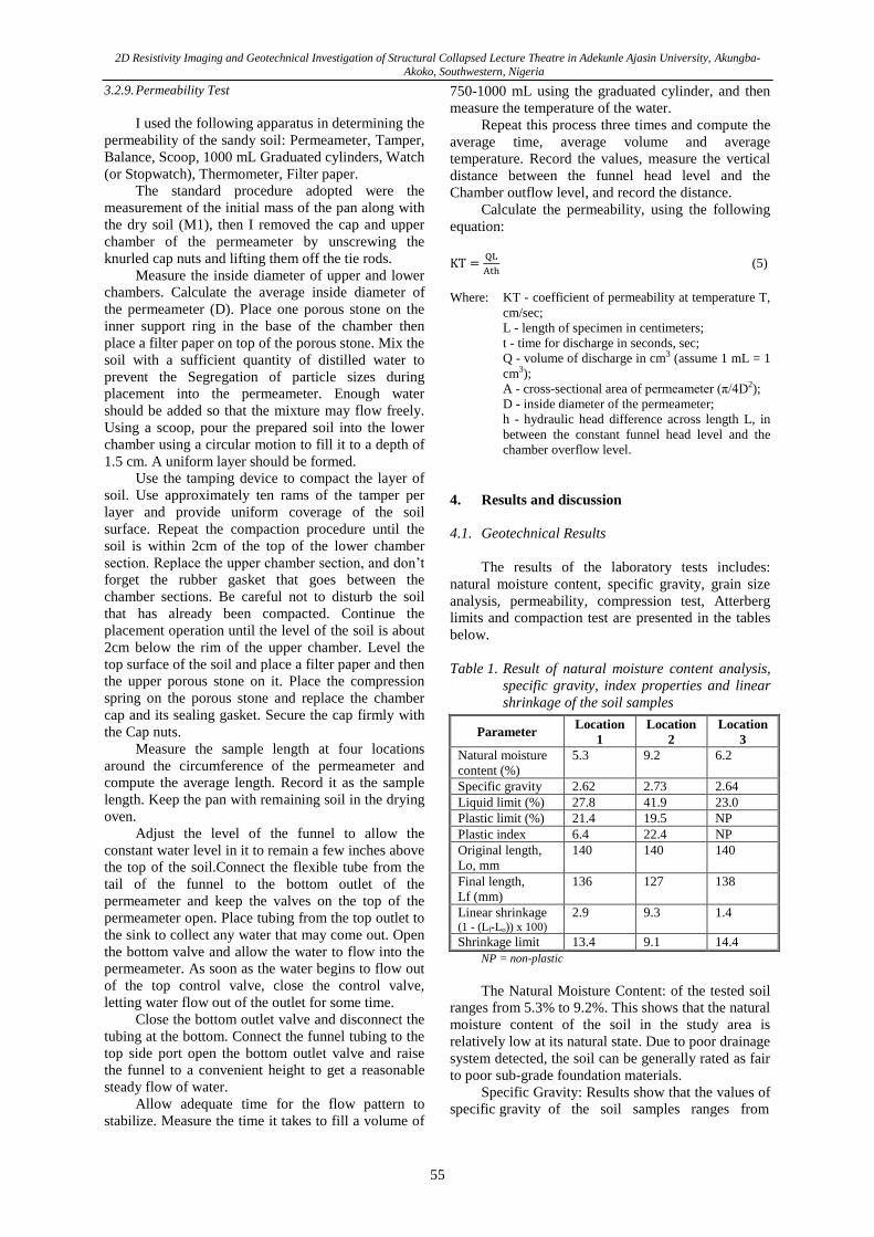
Table 1. Result of natural moisture content analysis,

specific gravity, index properties and linear

shrinkage of the soil samples

Parameter Location

1

Location

2

Location

3

Natural moisture

content (%)

5.3 9.2 6.2

Specific gravity 2.62 2.73 2.64

Liquid limit (%) 27.8 41.9 23.0

Plastic limit (%) 21.4 19.5 NP

Plastic index 6.4 22.4 NP

Original length,

Lo, mm

140 140 140

Final length,

Lf (mm)

136 127 138

Linear shrinkage (1 - (Lf-Lo)) x 100)

2.9 9.3 1.4

Shrinkage limit 13.4 9.1 14.4

NP = non-plastic

The Natural Moisture Content: of the tested soil

ranges from 5.3% to 9.2%. This shows that the natural

moisture content of the soil in the study area is

relatively low at its natural state. Due to poor drainage

system detected, the soil can be generally rated as fair

to poor sub-grade foundation materials.

Specific Gravity: Results show that the values of

specific gravity of the soil samples ranges from

Cyril C. Okpoli

56

2.620 and 2.730. Therefore, the failed building in the

study area is due to poor drainage network.

Atterberg Limits: As shown in Table1, the

Liquid Limit of the soil samples ranges from 23.0-

41.7%. The Plastic Limit ranges from not plastic-

21.4%, and the corresponding Plasticity Index ranges

from not- plastic 22.4%. The tested soil samples are

of medium consistency limits indicating low

percentage of clay content in the soil. Generally, soils

having high values of liquid and plastic limits are

considered poor as foundation materials. The

plasticity index of sample no 1 & 3 is lower than 20%

maximum which Federal Ministry of Works and

Housing (FMWH) (1972) recommended, hence it

shows a poor engineering property since the higher

the plastic index of a soil, the lesser the competency

of the soil as a foundation material. While that of

sample no 2 is higher than the maximum value,

therefore it is less competence as a good foundation

material. Table 1: The index properties of the soil

samples

The linear shrinkage: value of the tested soils

ranges from 1.4-9.3% (Table 1). Brink, (1992)

suggested that soils with linear shrinkage less or

higher than 8% would not be good as foundation

material. The linear shrinkage of sample no 1 & 3 is

less than 8% recommended, hence not good as

foundation materials. While the linear shrinkage of

sample no 2 is greater than 8%, hence the soils is

likely to be subjective to swelling and shrinkage

during alternate dry and wet seasons of the humid

tropical climatic condition of the south western

Nigeria. This must be taken into cognizance in the

design of the foundation.

The maximum dry density (MDD) and optimum

moisture content (OMC) of the soils ranges between

1790-2124kg/m3 and 9.1-18.2% respectively. These

values show that, the soils respond gradually to

compaction. The importance of compaction is to

improve the desirable load bearing properties of soil

as a foundation material.

Table 2. Showing compaction test results

Sample

Number

Compaction MDD

(Kg/m3)

Parameter

OMC (%)

Location 1 2114 9.9

Location 2 1790 18.2

Location 3 2124 9.1

The degree of permeability of location one is

low, this signifies that the drainage condition of the

area is fair, while the degree of permeability of

location two is very low, this signifies that the

drainage condition is poor, and the degree of

permeability of location three is medium, signifying

fair drainage system in the area.

Table 3. Showing results for permeability test

Sample

number

Permeability test Degree of

permeability

Location 1 8.0 x 10-5 Low

Location 2 8.1 x 10-7 Very low

Location 3 1.0 x 10-4 Medium

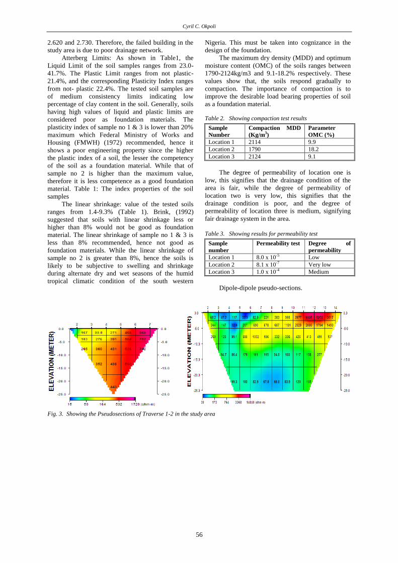
Dipole-dipole pseudo-sections.

Fig. 3. Showing the Pseudosections of Traverse 1-2 in the study area

2D Resistivity Imaging and Geotechnical Investigation of Structural Collapsed Lecture Theatre in Adekunle Ajasin University, Akungba-

Akoko, Southwestern, Nigeria

57

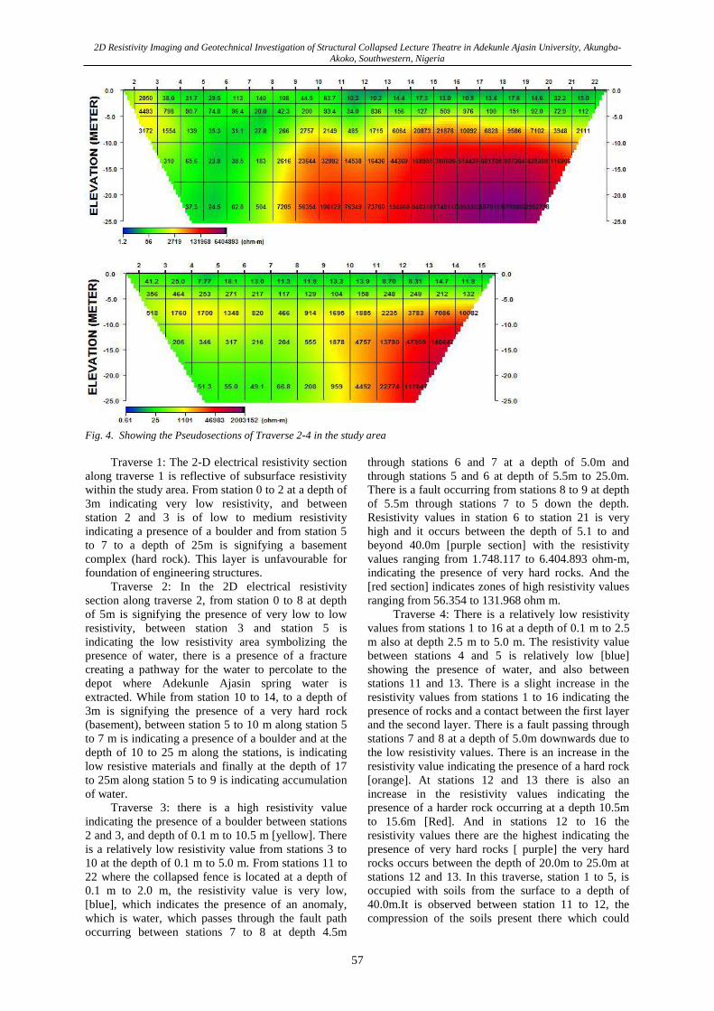
Fig. 4. Showing the Pseudosections of Traverse 2-4 in the study area

Traverse 1: The 2-D electrical resistivity section

along traverse 1 is reflective of subsurface resistivity

within the study area. From station 0 to 2 at a depth of

3m indicating very low resistivity, and between

station 2 and 3 is of low to medium resistivity

indicating a presence of a boulder and from station 5

to 7 to a depth of 25m is signifying a basement

complex (hard rock). This layer is unfavourable for

foundation of engineering structures.

Traverse 2: In the 2D electrical resistivity

section along traverse 2, from station 0 to 8 at depth

of 5m is signifying the presence of very low to low

resistivity, between station 3 and station 5 is

indicating the low resistivity area symbolizing the

presence of water, there is a presence of a fracture

creating a pathway for the water to percolate to the

depot where Adekunle Ajasin spring water is

extracted. While from station 10 to 14, to a depth of

3m is signifying the presence of a very hard rock

(basement), between station 5 to 10 m along station 5

to 7 m is indicating a presence of a boulder and at the

depth of 10 to 25 m along the stations, is indicating

low resistive materials and finally at the depth of 17

to 25m along station 5 to 9 is indicating accumulation

of water.

Traverse 3: there is a high resistivity value

indicating the presence of a boulder between stations

2 and 3, and depth of 0.1 m to 10.5 m [yellow]. There

is a relatively low resistivity value from stations 3 to

10 at the depth of 0.1 m to 5.0 m. From stations 11 to

22 where the collapsed fence is located at a depth of

0.1 m to 2.0 m, the resistivity value is very low,

[blue], which indicates the presence of an anomaly,

which is water, which passes through the fault path

occurring between stations 7 to 8 at depth 4.5m

through stations 6 and 7 at a depth of 5.0m and

through stations 5 and 6 at depth of 5.5m to 25.0m.

There is a fault occurring from stations 8 to 9 at depth

of 5.5m through stations 7 to 5 down the depth.

Resistivity values in station 6 to station 21 is very

high and it occurs between the depth of 5.1 to and

beyond 40.0m [purple section] with the resistivity

values ranging from 1.748.117 to 6.404.893 ohm-m,

indicating the presence of very hard rocks. And the

[red section] indicates zones of high resistivity values

ranging from 56.354 to 131.968 ohm m.

Traverse 4: There is a relatively low resistivity

values from stations 1 to 16 at a depth of 0.1 m to 2.5

m also at depth 2.5 m to 5.0 m. The resistivity value

between stations 4 and 5 is relatively low [blue]

showing the presence of water, and also between

stations 11 and 13. There is a slight increase in the

resistivity values from stations 1 to 16 indicating the

presence of rocks and a contact between the first layer

and the second layer. There is a fault passing through

stations 7 and 8 at a depth of 5.0m downwards due to

the low resistivity values. There is an increase in the

resistivity value indicating the presence of a hard rock

[orange]. At stations 12 and 13 there is also an

increase in the resistivity values indicating the

presence of a harder rock occurring at a depth 10.5m

to 15.6m [Red]. And in stations 12 to 16 the

resistivity values there are the highest indicating the

presence of very hard rocks [ purple] the very hard

rocks occurs between the depth of 20.0m to 25.0m at

stations 12 and 13. In this traverse, station 1 to 5, is

occupied with soils from the surface to a depth of

40.0m.It is observed between station 11 to 12, the

compression of the soils present there which could

Cyril C. Okpoli

58

also be as a result of faulting of the hard rock present

beneath.

5. Conclusion

The geotechnical investigation and the

Geophysical surveying involving 2-D dipole-dipole

imaging, was carried out at the study area. The 2-D

dipole-dipole imaging, it was discovered that the top

soil is within the depth of 0 to 5m, it was also

discovered that resistivity values varies, with low

resistivity values characterizing the presence of

anomalies such as water and weathered layers. From

these results it could also be presumed that the failed

segments of the building under investigation are

presumably underlined by very hard rock which is

jointed/ faulted. This zone is characterized by very

high resistivity values, which is typical of very hard

rocks. The soils samples are generally of relatively

low natural moisture content. It has relatively low

clay content, which are generally less than 35%

recommended. Plasticity characteristics of the soil

samples reveal that the soil samples can be considered

as poor, based on the comparison of their plasticity

values with values specified by the Federal Ministry

of Works and Housing [1974]. The linear shrinkage of

the soil samples indicates poor, thereby has every

tendency to exhibit compaction problem. Grain size

distribution characteristics of the soil showed that the

soil is poorly sorted. This property limits the aptness

of the soil as building construction material. The

compaction classification after Wood’s system shows

that the soil samples present in location two is poor

for any engineering construction. Hence, the

structural collapse of the Lecture Theatre is due to:

excessive settlement of the soil materials on which it

was founded and jointing/faulting of hard rocks

leading to percolation and accumulation of water

present in the subsurface upon which the structure

was founded.

References

Aizebeokhai A.P, Olayinka A.I., Singh V.S. (2010).

Application of 2D and 3D geoelectrical resistivity imaging

for engineering site investigation in a crystalline basement

terrain, southwestern Nigeria. Journal. Environ. Earth

Science., doi.1007/s 12665-010-0474-z, p.1481.

Ajibade A.C. Woakes, M and Rahaman, M.A. 1989;

Proterozoic Crustal Development in the Pan-Africa Regime

of Nigeria, (Second Revised Edition by Kogbe C.A.). Rock

View Nigeria Limited, Jos, Nigeria, pp 57-69.

Binley A, Cassiani G, Middleton R, Winship P.,

(2002). Vadose zone flow model parameterization using

cross-borehole radar and resistivity imaging. Journal of

Hydrology, 267: 147-159. http://dx.doi.org/10.1016/S0022-

1694(02)00146-4

Brink A.B.A., Parridge J.C. and Williams A.A.B.

(1992). Soil Survey for Engineering, Claredon, Oxford.

Causes of Structural Failure Using Electrical Resistivity

Tomography (ERT): A Case Study of Lagos, Southwestern,

Nigeria. Miner. Wealth 156:7- 18.

Dahlin T ., Loke M.H. (1998). Resolution of 2D

wenner resistivity imaging as assessed by numerical

modelling. Journal of Applied Geophysics., 38(4): 237-248.

http://dx.doi.org/10.1016/S0926-9851(97)00030-X

Donald, V. and Cohen. P.E. (1998). “Inspecting Block

Foundation”. American Society of Home Inspectors ASH.

Reporter. December, 1998.

Federal ministry of works and housing (FMWH)

1994. General guidelines for building construction. 1:pp.

87-93.

Federal surveys. 1976. Highway Manual Part 1 Road

Design, Federal Ministry of Works and Housing. 1: pp 5-11.

Loke M.H., Acworth I. and Darlin T, (2003). A

comparison of smooth and blocky inversion methods in 2-D

electrical imaging surveys: Exploration Geophysics, 34,

182-187. http://dx.doi.org/10.1071/EG03182

Mesida E. A. (1987). Engineering Geophysics and its

Application in Engineering Site Investigations (Case study

from Ile –Ife Area). Journal of the Nigerian Engineer. 22(

2): 2005, pp. 59-65.

Olayinka A.I. (1999). Advantage of two-dimensional

geoelectrical imaging for groundwater prospecting: Case

study from Ira, southwestern Nigeria. Journal of National

Association of Hydrogeologist, 10: 55-61.

Ranjan O.R and Roa J.P. 2000. Roadwork; theory and

practice. 4th ed. Butterworth-Heinemann, Oxford. pp: 309.

Sands T.B. (2006). “Buildings Stability and Tree

Growth for in Swelling London Clay: Implications for Pile

Foundation Design”. www.agu.org.

Tomlinson M.J., Boorman R. (1978). Foundation

Design and Construction. Longman Scientific and

Technical: Singapore. 1- 125.

Cyril Chibueze Okpoli – lecturer at Department of

Geology, Adekunle Ajasin University.

Address: Department of Geology, Adekunle

Ajasin University, Akungba-

Akoko, PMB 001, Ondo State,

Nigeria.

Tel.: +2348064488625

E-mail: [email protected]

2D Resistivity Imaging and Geotechnical Investigation of Structural Collapsed Lecture Theatre in Adekunle Ajasin University, Akungba-

Akoko, Southwestern, Nigeria

59

Varža 2D formatu ir geotechniniai struktūrinių trūkių tyrimai

Adekunlo Ajasin universitete, Nigerijoje

Cyril Chibueze Okpoli Geologijos fakultetas, Adekunle Ajasin Universitetas, Akungba - Akokas, Ondo valstija, Nigerija

(gauta 2013 m. rugsėjo mėn., priimtas spaudai 2014 m. rugsėjo mėn.)

Geotechniniai ir geofiziniai tyrimai, apimantys elektros varžos matavimus ir laboratorinius tyrimus,

buvo atlikti su mėginiais, surinktais trijose skirtingose tiriamosios vietovės dalyse. Studijos pagrindinis tikslas

buvo įvertinti paviršinių dirvožemio medžiagų savybes. Tyrimui buvo pritaikyta elektros varžos tomografija,

naudojant „dipolis-dipolis“ konfigūraciją bei dirvožemio analizių technikas. Iš viso tyrime buvo naudojami

keturi traverso ir trys dirvožemio mėginiai.

Geofizinių tyrimų metu buvo nustatyta, kad viršutiniame dirvos sluoksnyje (nuo 0 iki 5 m gylyje) yra

kintanti varža, tai, tikėtina, rodo, kad šioje vietoje dirvožemį sudaro mažos varžos medžiagos, tokios kaip

vanduo, kartu su labai nedidės varžos pamatiniu kompleksu, kuriame vanduo akumuliuojasi ir per kurį

filtruojasi. Dėl to tokio tipo dirvožemio sluoksniai tampa pavojingi inžinerinių statinių pamatams. Kaip

akivaizdus neigiamas bruožas, įtakojantis susiformavusį dirvožemio įdubimą, buvo pasirinktas geologinis

reiškinys – lūžis pamatinėje uolienoje. Geotechniniai rezultatai parodė, kad natūralaus drėgmės kiekio,

savitojo sunkio, skystumo ribų, plastiškumo ribų, plastiškumo rodiklio, linijinio išsėdimo, sutankinimo ir

pralaidumo vertės kito intervaluose 5.3-9.2%, 2.620-2.730%, 23.0-41.9%, ne plastinis iki 21.4%, nuo ne

plastinio iki 22.4%, 1.4-9.3,1790-2114 kg/m3, 9.1-9.9 bei nuo labai nedidelės iki vidutinio dydžio varžos. Dėl

to dirvožemį formuojančios medžiagos buvo nustatytos kaip santykinai prastos pamatinės medžiagos

tiriamojoje teritorijoje.