26th International Conference on DNA Computing and Molecular Programming DNA 26, September 14–17, 2020, Oxford, UK (Virtual Conference) Edited by Cody Geary Matthew J. Patitz LIPIcs – Vol. 174 – DNA 26 www.dagstuhl.de/lipics

Welcome message from author
This document is posted to help you gain knowledge. Please leave a comment to let me know what you think about it! Share it to your friends and learn new things together.
Transcript
26th International Conference onDNA Computing and MolecularProgramming
DNA 26, September 14–17, 2020, Oxford, UK (VirtualConference)
Edited by
Cody GearyMatthew J. Patitz
LIPIcs – Vo l . 174 – DNA 26 www.dagstuh l .de/ l ip i c s

Editors
Cody GearyInterdisciplinary Nanoscience Centre, University of Aarhus, [email protected]
Matthew J. PatitzDepartment of Computer Science and Computer Engineering,University of Arkansas, Fayetteville, AR, [email protected]
ACM Classification 2012Theory of computation → Models of computation; Applied computing → Molecular structural biology;Applied computing → Biological networks; Information systems → Information storage systems
ISBN 978-3-95977-163-4
Published online and open access bySchloss Dagstuhl – Leibniz-Zentrum für Informatik GmbH, Dagstuhl Publishing, Saarbrücken/Wadern,Germany. Online available at https://www.dagstuhl.de/dagpub/978-3-95977-163-4.
Publication dateSeptember, 2020
Bibliographic information published by the Deutsche NationalbibliothekThe Deutsche Nationalbibliothek lists this publication in the Deutsche Nationalbibliografie; detailedbibliographic data are available in the Internet at https://portal.dnb.de.
LicenseThis work is licensed under a Creative Commons Attribution 3.0 Unported license (CC-BY 3.0):https://creativecommons.org/licenses/by/3.0/legalcode.In brief, this license authorizes each and everybody to share (to copy, distribute and transmit) the workunder the following conditions, without impairing or restricting the authors’ moral rights:
Attribution: The work must be attributed to its authors.
The copyright is retained by the corresponding authors.
Digital Object Identifier: 10.4230/LIPIcs.DNA.2020.0
ISBN 978-3-95977-163-4 ISSN 1868-8969 https://www.dagstuhl.de/lipics

0:iii
LIPIcs – Leibniz International Proceedings in Informatics
LIPIcs is a series of high-quality conference proceedings across all fields in informatics. LIPIcs volumesare published according to the principle of Open Access, i.e., they are available online and free of charge.
Editorial Board
Luca Aceto (Chair, Gran Sasso Science Institute and Reykjavik University)Christel Baier (TU Dresden)Mikolaj Bojanczyk (University of Warsaw)Roberto Di Cosmo (INRIA and University Paris Diderot)Javier Esparza (TU München)Meena Mahajan (Institute of Mathematical Sciences)Dieter van Melkebeek (University of Wisconsin-Madison)Anca Muscholl (University Bordeaux)Luke Ong (University of Oxford)Catuscia Palamidessi (INRIA)Thomas Schwentick (TU Dortmund)Raimund Seidel (Saarland University and Schloss Dagstuhl – Leibniz-Zentrum für Informatik)
ISSN 1868-8969
https://www.dagstuhl.de/lipics
DNA 26


Contents
PrefaceCody Geary and Matthew J. Patitz . . . . . . . . . . . . . . . . . . . . . . . . . . . . . . . . . . . . . . . . . . . . . . . 0:vii
Steering Committee. . . . . . . . . . . . . . . . . . . . . . . . . . . . . . . . . . . . . . . . . . . . . . . . . . . . . . . . . . . . . . . . . . . . . . . . . . . . . . . . . 0:ix
Programm Committee. . . . . . . . . . . . . . . . . . . . . . . . . . . . . . . . . . . . . . . . . . . . . . . . . . . . . . . . . . . . . . . . . . . . . . . . . . . . . . . . . 0:x
Additional Reviewers. . . . . . . . . . . . . . . . . . . . . . . . . . . . . . . . . . . . . . . . . . . . . . . . . . . . . . . . . . . . . . . . . . . . . . . . . . . . . . . . . 0:xi
Organizing Committee for DNA 26. . . . . . . . . . . . . . . . . . . . . . . . . . . . . . . . . . . . . . . . . . . . . . . . . . . . . . . . . . . . . . . . . . . . . . . . . . . . . . . . . 0:xii
Sponsors. . . . . . . . . . . . . . . . . . . . . . . . . . . . . . . . . . . . . . . . . . . . . . . . . . . . . . . . . . . . . . . . . . . . . . . . . . . . . . . . . 0:xiii
Regular Papers
The Topology of Scaffold Routings on Non-Spherical Mesh WireframesAbdulmelik Mohammed, Nataša Jonoska, and Masahico Saito . . . . . . . . . . . . . . . . . . . . 1:1–1:17
Simplifying Chemical Reaction Network Implementations with Two-StrandedDNA Building Blocks
Robert F. Johnson and Lulu Qian . . . . . . . . . . . . . . . . . . . . . . . . . . . . . . . . . . . . . . . . . . . . . . . 2:1–2:14
Composable Computation in Leaderless, Discrete Chemical Reaction NetworksHooman Hashemi, Ben Chugg, and Anne Condon . . . . . . . . . . . . . . . . . . . . . . . . . . . . . . . . 3:1–3:18
CRNs Exposed: A Method for the Systematic Exploration of Chemical ReactionNetworks
Marko Vasic, David Soloveichik, and Sarfraz Khurshid . . . . . . . . . . . . . . . . . . . . . . . . . . . 4:1–4:25
Population-Induced Phase Transitions and the Verification of Chemical ReactionNetworks
James I. Lathrop, Jack H. Lutz, Robyn R. Lutz, Hugh D. Potter, andMatthew R. Riley . . . . . . . . . . . . . . . . . . . . . . . . . . . . . . . . . . . . . . . . . . . . . . . . . . . . . . . . . . . . . . . . 5:1–5:17
ALCH: An Imperative Language for Chemical Reaction Network-Controlled TileAssembly
Titus H. Klinge, James I. Lathrop, Sonia Moreno, Hugh D. Potter,Narun K. Raman, and Matthew R. Riley . . . . . . . . . . . . . . . . . . . . . . . . . . . . . . . . . . . . . . . . 6:1–6:22
Implementing Non-Equilibrium Networks with Active Circuits of Duplex CatalystsAntti Lankinen, Ismael Mullor Ruiz, and Thomas E. Ouldridge . . . . . . . . . . . . . . . . . . 7:1–7:25
Design Automation of Polyomino Set That Self-Assembles into a Desired ShapeYuta Matsumura, Ibuki Kawamata, and Satoshi Murata . . . . . . . . . . . . . . . . . . . . . . . . . . 8:1–8:15
26th International Conference on DNA Computing and Molecular Programming (DNA 26).Editors: Cody Geary and Matthew J. Patitz
Leibniz International Proceedings in InformaticsSchloss Dagstuhl – Leibniz-Zentrum für Informatik, Dagstuhl Publishing, Germany

0:vi Contents
scadnano: A Browser-Based, Scriptable Tool for Designing DNA NanostructuresDavid Doty, Benjamin L Lee, and Tristan Stérin . . . . . . . . . . . . . . . . . . . . . . . . . . . . . . . . 9:1–9:17
Verification and Computation in Restricted Tile AutomataDavid Caballero, Timothy Gomez, Robert Schweller, and Tim Wylie . . . . . . . . . . . . . 10:1–10:18
Turning MachinesIrina Kostitsyna, Cai Wood, and Damien Woods . . . . . . . . . . . . . . . . . . . . . . . . . . . . . . . . . 11:1–11:21
Preface
This volume contains the papers presented at DNA 26: the 26th International Conference onDNA Computing and Molecular Programming. The conference was originally scheduled tobe held at the University of Oxford, but due to the COVID-19 pandemic it was changed toan online format. The virtual conference was held during September 14-17, 2020, and wasorganized under the auspices of the International Society for Nanoscale Science, Computation,and Engineering (ISNSCE). The DNA conference series aims to draw together researchers fromthe fields of mathematics, computer science, physics, chemistry, biology, and nanotechnologyto address the analysis, design, and synthesis of information-based molecular systems.
Papers and presentations were sought in all areas that relate to biomolecular computing,including, but not restricted to: algorithms and models for computation on biomolecularsystems; computational processes in vitro and in vivo; molecular switches, gates, devices,and circuits; molecular folding and self-assembly of nanostructures; analysis and theoreticalmodels of laboratory techniques; molecular motors and molecular robotics; informationstorage; studies of fault-tolerance and error correction; software tools for analysis, simulation,and design; synthetic biology and in vitro evolution; and applications in engineering, physics,chemistry, biology, and medicine.
Authors who wished to orally present their work were asked to select one of two submissiontracks: Track A (full paper) or Track B (one-page abstract with supplementary document).Track B is primarily for authors submitting experimental results who plan to submit toa journal rather than publish in the conference proceedings. We received 52 submissionsfor oral presentations: 25 submissions to Track A and 27 submissions to Track B. Eachsubmission was reviewed by at least three reviewers, with several reviewed by four reviewers.The Program Committee accepted 11 papers for Track A (44%) and 11 papers for TrackB (41%). Additionally, the Program Committee reviewed and accepted 37 submissions toTrack C (poster) and selected 6 for short oral presentations. This volume contains the papersaccepted for Track A.
We express our sincere appreciation to our invited speakers, Tom de Greef, MartaKwiatkowska, Jérôme Leroux, Ard Louis, Damien Woods, and Niles Pierce. We especiallythank all of the authors who contributed papers to these proceedings, and who presentedpapers and posters during the conference. Last but not least, the editors thank the membersof the Program Committee and the additional invited reviewers for their hard work inreviewing the papers and providing constructive comments to the authors.
September 2020 Cody GearyMatt Patitz
26th International Conference on DNA Computing and Molecular Programming (DNA 26).Editors: Cody Geary and Matthew J. Patitz
Leibniz International Proceedings in InformaticsSchloss Dagstuhl – Leibniz-Zentrum für Informatik, Dagstuhl Publishing, Germany


Organization
Steering Committee
Luca Cardelli Oxford University, UKAnne Condon (Chair) University of British Columbia, CanadaMasami Hagiya University of Tokyo, JapanNatasha Jonoska University of Southern Florida, USALila Kari University of Waterloo, CanadaChengde Mao Purdue University, USASatoshi Murata Tohoku University, JapanJohn H. Reif Duke University, USAGrzegorz Rozenberg University of Leiden, The NetherlandsRebecca Schulman Johns Hopkins University, USANadrian C. Seeman New York University, USAFriedrich Simmel Technical University Munich, GermanyDavid Soloveichik University of Texas at Austin, USAAndrew J. Turberfield Oxford University, UKErik Winfree California Institute of Technology, USADamien Woods Maynooth University, IrelandHao Yan Arizona State University, USA
26th International Conference on DNA Computing and Molecular Programming (DNA 26).Editors: Cody Geary and Matthew J. Patitz
Leibniz International Proceedings in InformaticsSchloss Dagstuhl – Leibniz-Zentrum für Informatik, Dagstuhl Publishing, Germany

0:x Organization
Program Committee
Matt Patitz (Co-chair) University of Arkansas, USACody Geary (Co-chair) Aarhus University, DenmarkEbbe Andersen Aarhus University, DenmarkLuca Cardelli University of Oxford, UKYuan-Jyue Chen Microsoft Research, USAAnne Condon University of British Columbia, CanadaDavid Doty University of California, Davis, USAElisa Franco University of California, Los Angeles, USAAnthony Genot CNRS, FranceManoj Gopalkrishnan Indian Institute of Technology, Bombay, IndiaElton Graugnard Boise State University, USAMasami Hagiya University of Tokyo, JapanRizal Hariadi Arizona State University, USANatasha Jonoska University of South Florida, USALila Kari University of Waterloo, CanadaMatthew Lakin University of New Mexico, USAChenxiang Lin Yale University, USAYan Liu Arizona State University, USAOlgica Milenkovic University of Illinois, USASatoshi Murata Tohoku University, JapanPekka Orponen Aalto University, FinlandTom Ouldridge Imperial College London, UKLulu Qian California Institute of Technology, USAJohn Reif Duke University, USADominic Scalise Johns Hopkins University, USANicolas Schabanel CNRS and École normale supérieure de Lyon, FranceJoseph Schaeffer Autodesk Research, USARobbie Schweller University of Texas Rio Grande Valley, USAWilliam Shih Harvard University, USADavid Soloveichik University of Texas, USADarko Stefanovic University of New Mexico, USAJamie Stewart California Institute of Technology, USAPetr Sulc Arizona State University, USAChris Thachuk California Institute of Technology, USAGreg Tikhomirov California Institute of Technology, USAAndrew Turberfield Oxford University, UKBryan Wei Tsinghua University, ChinaShelley Wickham University of Sydney, AustraliaErik Winfree California Institute of Technology, USADamien Woods Maynooth University, IrelandFei Zhang Rutgers University, USA

Organization 0:xi
Additional Reviewers
Abdulmelik Mohammed Joanna Ellis-MonaghanChristian Cuba Samaniego Lance WilliamsDaniel Fu Margherita Maria FerrariDaniel Hader Miklos Z. RaczDavid Arredondo Scott SummersDavid Haley Shalin ShahEric Severson Shinnosuke SekiEugen Czeizler Tianqi SongHo-Lin Chen Wen Wang
DNA 26

0:xii Organization
Organizing Committee for DNA 26
Andrew Phillips (Co-chair) Microsoft Research, Cambridge, UKAndrew Turberfield (Co-chair) University of Oxford, UKClaire Garland Institute of Physics, UK

Organization 0:xiii
Sponsors
International Society for Nanoscale Science, Computation, and EngineeringBiological Physics Group, Institute of PhysicsDepartment of Physics, University of OxfordMicrosoft Research
DNA 26


The Topology of Scaffold Routings onNon-Spherical Mesh WireframesAbdulmelik MohammedDepartment of Mathematics and Statistics, University of South Florida, Tampa, FL, [email protected]
Nataša JonoskaDepartment of Mathematics and Statistics, University of South Florida, Tampa, FL, [email protected]
Masahico SaitoDepartment of Mathematics and Statistics, University of South Florida, Tampa, FL, [email protected]
AbstractThe routing of a DNA-origami scaffold strand is often modelled as an Eulerian circuit of an Euleriangraph in combinatorial models of DNA origami design. The knot type of the scaffold strand dictatesthe feasibility of an Eulerian circuit to be used as the scaffold route in the design. Motivated by thetopology of scaffold routings in 3D DNA origami, we investigate the knottedness of Eulerian circuitson surface-embedded graphs. We show that certain graph embeddings, checkerboard colorable,always admit unknotted Eulerian circuits. On the other hand, we prove that if a graph admits anembedding in a torus that is not checkerboard colorable, then it can be re-embedded so that all itsnon-intersecting Eulerian circuits are knotted. For surfaces of genus greater than one, we presentan infinite family of checkerboard-colorable graph embeddings where there exist knotted Euleriancircuits.
2012 ACM Subject Classification Mathematics of computing → Discrete mathematics
Keywords and phrases DNA origami, Scaffold routing, Graphs, Surfaces, Knots, Eulerian circuits
Digital Object Identifier 10.4230/LIPIcs.DNA.2020.1
Funding This research was (partially) supported by the grants NSF DMS-1800443/1764366 and theSoutheast Center for Mathematics and Biology, an NSF-Simons Research Center for Mathematicsof Complex Biological Systems, under National Science Foundation Grant No. DMS-1764406 andSimons Foundation Grant No. 594594. Travel support is provided to Abdulmelik Mohammedthrough an AMS-Simons Travel Grant (2020).
1 Introduction
The conception of stable branched DNA molecules was one of the central ideas in the birthof DNA nanotechnology [28, 29]. Branched nucleic acids exhibit a mathematical structurenaturally modelled by graphs, where graph vertices (roughly points) correspond to thebranch locations while graph edges (roughly line segments connecting points) model lineardouble-helical domains. Graph-theoretic models for the construction of three-dimensionalDNA nanostructures have been proposed as early as 1997 [15, 16]. The first experimentsdemonstrating the self-assembly of non-regular graphs using DNA junctions as vertices andduplexes as edge connectors were presented in 2003 [27]. DNA self assembly has also beenused to solve small instances of graph-theoretic problems such as the Directed HamiltonPath problem [2] and the vertex 3-colorability problem [33].
Graphs of convex polyhedra [8, 11, 13, 14, 30] have been synthesized using a varietyof DNA vertex and edge motifs. Graph theory took an explicit and integral role in theautomated design of non-convex polyhedra when graphs embedded in topological spheres were
© Abdulmelik Mohammed, Nataša Jonoska, and Masahico Saito;licensed under Creative Commons License CC-BY
26th International Conference on DNA Computing and Molecular Programming (DNA 26).Editors: Cody Geary and Matthew J. Patitz; Article No. 1; pp. 1:1–1:17
Leibniz International Proceedings in InformaticsSchloss Dagstuhl – Leibniz-Zentrum für Informatik, Dagstuhl Publishing, Germany

1:2 The Topology of Scaffold Routings on Non-Spherical Mesh Wireframes
Figure 1 A knotted Eulerian circuit (A-trail) on a torus.
exploited to model a large class of wireframe DNA origami [5, 22]. Thereafter, graph-theoreticmodelling has been widely adopted for the design and synthesis of 2D [4, 18, 19] and 3Dwireframe DNA origami [17, 32].
In DNA origami [26], a long, typically circular, scaffold strand is folded into a targetconformation using hundreds of short helper strands. One of the key and challenging stepsin designing complex 3D DNA origami is the routing of the circular scaffold strand so that itcovers half the mass of each of the constituent helical domains. In graph based design ofDNA origami [5, 4, 32], the scaffold routing typically corresponds to an Eulerian circuit of agraph which has been obtained from the target wireframe after some processing. Briefly, anEulerian circuit is a closed path in a graph which traces each edge exactly once. Euleriancircuits capture the essential idea that the scaffold constitutes exactly one of the strands ineach double helical domain. A general scheme for stapling Eulerian scaffold routings hasbeen proposed in [22].
A fundamental consideration when employing circular strands in the design of nano-structures is ensuring that the topology of the strand routing in the design correspondsto the topology of the physical strand. For instance, the scaffold strand currently used inDNA origami assembly is unknotted. In most DNA origami constructs, the scaffold doesnot intersect itself when it traces the structure. For this reason, a class of non-intersectingEulerian circuits called A-trails was adopted for unknotted scaffold routing of Eulerian graphsembedded in a sphere [5]. However, it has been pointed out that A-trails can be knottedfor graphs embedded in tori [9]. An example of a knotted A-trail on a torus is shown inFigure 1. The A-trail is illustrated with the blue curve. As usual, the torus is obtainedby gluing the horizontal boundaries in red together to form a cylinder and then gluing theviolet boundaries to close the cylinder to a torus. Compare with Figure 3 to see that theA-trail corresponds to a trefoil knot. Unknotted scaffold routings may be achieved withnon-intersecting Eulerian circuits (a generalization of A-trails, see definitions in Section 2) forgraphs that are embedded in surfaces. In this paper, we further investigate the knottedness ofnon-intersecting Eulerian circuits. These Eulerian circuits can represent knotted or unknottedscaffold routings. Here we specify properties of graph embeddings in surfaces when knottedor unknotted scaffold routings arise from non-intersecting Eulerian circuits.
An approximation algorithm for finding unknotted scaffold routings on triangular embed-dings in positive genus surfaces has been proposed earlier [23]. For certain Eulerian graphs,the algorithm can trace some edges twice even if the embedded graph contains an unknottednon-intersecting Eulerian circuit. It has been proved that for checkerboard-colorable graphembeddings (see definition in Section 2) in a torus, A-trails, if any exist, are unknotted [24].In this paper, we present a number of additional results connecting checkerboard-colorablegraph embeddings and the knottedness of non-intersecting Eulerian circuits. We generalizethe result of [24] by proving that all non-intersecting Eulerian circuits of checkerboard-colorable torus graphs are unknotted. We show that at least one unknotted non-intersecting

A. Mohammed, N. Jonoska, and M. Saito 1:3
(a) (b) (c)
Figure 2 Closed orientable surfaces of genus 1, 2 and 3 in (a), (b) and (c), respectively.
Eulerian circuits exists for all checkerboard-colorable embeddings in orientable closed surfaces,including surfaces of genus greater than one. We show that, however, checkerboard-colorablegraph embeddings in surfaces of genus greater than one can contain knotted Eulerian circuits.For tori, we characterize graphs which admit embeddings where all non-intersecting Euleriancircuits are knotted; such embeddings would require a knotted scaffold for routing as anon-intersecting Eulerian circuit.
2 Preliminaries
Graphs embedded in non-spherical surfaces significantly expand the class of wireframe DNAorigami that can be designed based on topological techniques. For instance, reinforcedcubes [32] and certain cubic lattices can be modelled as graphs on non-spherical surfaces. Inthis section, we present the basic topological concepts needed to introduce non-intersectingEulerian circuits on surface-embedded graphs, our model for topological study of scaffoldroutings. We refer the reader to Armstrong’s book [3] for an accessible account on surfaces,the monograph by Fleischner [10] for a detailed exposition on Eulerian graphs and the firsttwo chapters of Rolfsen’s classic [25] for an illustrative introduction to knot theory.
2.1 SurfacesSurfaces are mathematical models of spaces which, when sufficiently zoomed in, look likea flat plane. Surfaces are commonly used in computer graphics as boundary models ofwell-defined 3D shapes. The simplest example of a surface is the unit sphere S2 = (x, y, z) ∈R3|x2 + y2 + z2 = 1. Topologically, a sphere is any space homeomorphic to the unit sphere.For instance, the underlying spaces of all the meshes constructed in [5] are topological spheres.
The simplest surface topologically distinct from a sphere is a torus. It is commonlyrecognized in its standard embedding like the crust of a doughnut (cf. Figure 2a). A toruscan be fairly complicated as a geometric figure. The surface of a regular coffee mug is, forinstance, topologically a torus. Let S1 denote the unit circle in the plane. Formally, a torus Tis a surface homeomorphic to the product space S1×S1. Viewing S1 as the unit circle in thecomplex plane, points in a torus can be given coordinates (eiθ, eiφ), for 0 ≤ θ, φ < 2π. In thestandard embedding of the torus (Figure 2a), θ can be understood as the counter-clockwiserotation with respect to the axis of rotational symmetry, while φ denotes the right-handedrotation with respect to the core circle of the embedding. A torus is commonly representedby its fundamental polygon, a square whose parallel edges are identified and glued to formthe torus (compare Figure 3c and 3b). On the square, θ can be understood to go from 0 to2π along the horizontal edge in the positive x direction, while φ does so along the verticaledge in the positive y direction.
More complicated surfaces are constructed by joining tori together as follows. Theconnected sum of two surfaces F1 and F2 is obtained by removing topological open disksDi from Fi, for i ∈ 1, 2, and gluing the resulting surfaces Fi \Di along their boundaries.For instance, the connected sum of two tori is the 2-torus shown in Figure 2b; the blue
DNA 26
1:4 The Topology of Scaffold Routings on Non-Spherical Mesh Wireframes
(a) (b) (c)
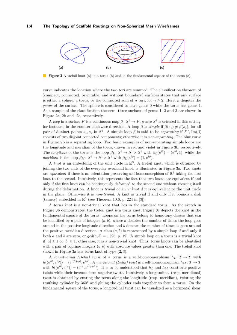
Figure 3 A trefoil knot (a) in a torus (b) and in the fundamental square of the torus (c).
curve indicates the location where the two tori are summed. The classification theorem of(compact, connected, orientable, and without boundary) surfaces states that any surfaceis either a sphere, a torus, or the connected sum of n tori, for n ≥ 2. Here, n denotes thegenus of the surface. The sphere is considered to have genus 0 while the torus has genus 1.As a sample of the classification theorem, three surfaces of genus 1, 2 and 3 are shown inFigure 2a, 2b and 2c, respectively.
A loop in a surface F is a continuous map β : S1 → F , where S1 is oriented in this setting,for instance, in the counter-clockwise direction. A loop β is simple if β(s1) 6= β(s2), for allpair of distinct points s1, s2 in S1. A simple loop β is said to be separating if F \ Im(β)consists of two disjoint connected components; otherwise it is non-separating. The blue curvein Figure 2b is a separating loop. Two basic examples of non-separating simple loops arethe longitude and meridian of the torus, drawn in red and violet in Figure 3b, respectively.The longitude of the torus is the loop βL : S1 → S1 × S1 with βL(eiθ) = (eiθ, 1), while themeridian is the loop βM : S1 → S1 × S1 with βL(eiφ) = (1, eiφ).
A knot is an embedding of the unit circle in R3. A trefoil knot, which is obtained byjoining the two ends of the everyday overhand knot, is illustrated in Figure 3a. Two knotsare equivalent if there is an orientation preserving self-homeomorphism of R3 taking the firstknot to the second. Intuitively, this represents the fact that two knots are equivalent if andonly if the first knot can be continuously deformed to the second one without crossing itselfduring the deformation. A knot is trivial or an unknot if it is equivalent to the unit circlein the plane. Otherwise it is non-trivial. A knot is trivial if and only if it bounds a disk(tamely) embedded in R3 (see Theorem 10.6, p. 224 in [3]).
A torus knot is a non-trivial knot that lies in the standard torus. As the sketch inFigure 3b demonstrates, the trefoil knot is a torus knot; Figure 3c depicts the knot in thefundamental square of the torus. Loops on the torus belong to homotopy classes that canbe identified by a pair of integers (a, b), where a denotes the number of times the loop goesaround in the positive longitude direction and b denotes the number of times it goes aroundthe positive meridian direction. A class (a, b) is represented by a simple loop if and only ifboth a and b are zero, or gcd(a, b) = 1 [25, p. 19]. A simple loop on a torus is a trivial knotif |a| ≤ 1 or |b| ≤ 1; otherwise, it is a non-trivial knot. Thus, torus knots can be identifiedwith a pair of coprime integers (a, b) with absolute values greater than one. The trefoil knotshown in Figure 3a is a torus knot of type (2, 3).
A longitudinal (Dehn) twist of a torus is a self-homeomorphism hL : T → T withh((eiθ, eiφ)) = (ei(θ+φ), eiφ). A meridional (Dehn) twist is a self-homeomorphism hM : T → T
with h((eiθ, eiφ)) = (eiφ, ei(φ+θ)). It is to be understood that hL and hM constitute positivetwists while their inverses form negative twists. Intuitively, a longitudinal (resp. meridional)twist is obtained by cutting the torus along the longitude (resp. meridian), twisting theresulting cylinder by 360 and gluing the cylinder ends together to form a torus. On thefundamental square of the torus, a longitudinal twist can be visualized as a horizontal shear,
A. Mohammed, N. Jonoska, and M. Saito 1:5
(a) (b)
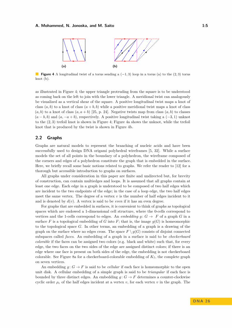
Figure 4 A longitudinal twist of a torus sending a (−1, 3) loop in a torus (a) to the (2, 3) torusknot (b).
as illustrated in Figure 4; the upper triangle protruding from the square is to be understoodas coming back on the left to join with the lower triangle. A meridional twist can analogouslybe visualized as a vertical shear of the square. A positive longitudinal twist maps a knot ofclass (a, b) to a knot of class (a+ b, b) while a positive meridional twist maps a knot of class(a, b) to a knot of class (a, a+ b) [25, p. 24]. Negative twists map from class (a, b) to classes(a− b, b) and (a,−a+ b), respectively. A positive longitudinal twist taking a (−3, 1) unknotto the (2, 3) trefoil knot is shown in Figure 4; Figure 4a shows the unknot, while the trefoilknot that is produced by the twist is shown in Figure 4b.
2.2 GraphsGraphs are natural models to represent the branching of nucleic acids and have beensuccessfully used to design DNA origami polyhedral wireframes [5, 32]. While a surfacemodels the set of all points in the boundary of a polyhedron, the wireframe composed ofthe corners and edges of a polyhedron constitute the graph that is embedded in the surface.Here, we briefly recall some basic notions related to graphs. We refer the reader to [12] for athorough but accessible introduction to graphs on surfaces.
All graphs under consideration in this paper are finite and undirected but, for brevityof construction, can contain multiedges and loops. It is assumed that all graphs contain atleast one edge. Each edge in a graph is understood to be composed of two half edges whichare incident to the two endpoints of the edge; in the case of a loop edge, the two half edgesmeet the same vertex. The degree of a vertex v is the number of half edges incident to itand is denoted by d(v). A vertex is said to be even if it has an even degree.
For graphs that are embedded in surfaces, it is convenient to think of graphs as topologicalspaces which are endowed a 1-dimensional cell structure, where the 0-cells correspond tovertices and the 1-cells correspond to edges. An embedding g : G → F of a graph G in asurface F is a topological embedding of G into F ; that is, the image g(G) is homeomorphicto the topological space G. In other terms, an embedding of a graph is a drawing of thegraph on the surface where no edges cross. The space F \ g(G) consists of disjoint connectedsubspaces called faces. An embedding of a graph in a surface is said to be checkerboardcolorable if the faces can be assigned two colors (e.g. black and white) such that, for everyedge, the two faces on the two sides of the edge are assigned distinct colors; if there is anedge where one face is present on both sides of the edge, the embedding is not checkerboardcolorable. See Figure 8a for a checkerboard-colorable embedding of K7, the complete graphon seven vertices.
An embedding g : G→ F is said to be cellular if each face is homeomorphic to the openunit disk. A cellular embedding of a simple graph is said to be triangular if each face isbounded by three distinct edges. An embedding g : G→ F determines a counter-clockwisecyclic order ρv of the half edges incident at a vertex v, for each vertex v in the graph. The
DNA 26

1:6 The Topology of Scaffold Routings on Non-Spherical Mesh Wireframes
v
b2
b1
(a)
w u
b2
b1
(b) (c) (d) (e)
Figure 5 Smoothing of an even vertex. (a) Neighboring half edges in a vertex, (b) smoothingone transition composed of the neighboring half edges, (c) a smoothing of the vertex induced bya non-intersecting Eulerian circuit, (d) a smoothing induced by an A-trail, (e) a splitting away oftransitions where two transitions intersect.
order ρv is called a rotation at v. The collection ρ = ρv : v ∈ G of rotations at vertices iscalled a rotation system. In a rotation system, each vertex can be treated as rigid (see [7]for the notion of rigid vertices). Conversely, if each vertex is rigid, it gives rise to a cellularembedding g : G→ F for some (closed orientable) surface F .
In wireframe DNA origami [5, 32], the fact that the scaffold comprises one strand of eachdouble-helical domain is conveniently captured by an Eulerian circuit of an underlying graph.A circuit in a graph is a closed walk (v0, e0, v1, . . . , vl−1, el−1, v0) with no repeated edges,where l ≥ 1 is the length of the circuit and each ei, for 0 ≤ i ≤ l − 1, is an edge in the graphwith endpoints vi, vi+1 mod l. An Eulerian circuit is a circuit which visits every edge of thegraph. A graph is said to be Eulerian if it contains an Eulerian circuit. A connected graphis Eulerian if and only if every vertex is of even degree. Closely related to circuits are cyclesand transitions. A cycle is a circuit with no repeated vertices. For a surface-embedded graph,a cycle corresponds to a simple loop and the separating/non-separating qualification equallyapply to cycles. A transition is an unordered pair of half edges incident to a common vertex.A circuit C = (v0, e0, v1, . . . , vl−1, el−1, v0) can also be seen as a collection of transitionsbi, b′i+1 mod l, where bi is the half edge of ei incident to vi+1 mod l, and b′i is the half edgeof ei incident with vi, for all i ∈ 0, . . . , l − l. In this sense, we can say that bi, b′i+1 mod lis contained in C.
Let g : G→ F be an embedding of a graph in a surface. Let v be a vertex ofG with d(v) ≥ 4and let the rotation ρv determined by g be (b0, . . . , bd(v)−1). Let 0 ≤ i, j, k, l ≤ d(v)− 1 withi < j, k < l, i < k. A pair of disjoint transitions bi, bj, bk, bl intersect if i < k < j < l
(cf. Figure 5e). An Eulerian circuit of an Eulerian graph G is said to be non-intersectingwith respect to g : G → F if it contains no intersecting transitions with respect to g (cf.the collection of transitions of the vertex v in Figure 5a suggested by Figure 5c). It hasbeen shown that a non-intersecting Eulerian circuit can be found in polynomial time for anyEulerian graph embedded in a sphere [1, 31], or in any other surface [10, 23]. However, thecomputational complexity changes when considering a subclass of non-intersecting Euleriancircuits called A-trails. Two half edges b1, b2 incident to a vertex v are said to be neighborsif ρv(b1) = b2 or ρv(b2) = b1 (see Figure 5a for an example). An A-trail is a non-intersectingEulerian circuit where every transition is composed of neighboring half edges (cf. Figure 5d).Deciding whether a surface-embedded graph has an A-trail is known to be NP-complete,even when restricted to embeddings in a sphere [6].
Let g : G→ F be a graph embedded in a surface. Let v be a vertex of G, d(v) ≥ 4, withrotation ρv determined by g. Let t = b1, b2 be a transition composed of neighboring halfedges incident to v. A smoothing of a transition t is the graph embedded in F obtainedfrom (G, g) by deleting v and adding two new vertices u and w such that b1 and b2 becomeincident with u and the rest of the half edges become incident with w. The graph obtained

A. Mohammed, N. Jonoska, and M. Saito 1:7
after smoothing is embedded exactly according to g except in a local disk neighborhood of vwhere u and w are embedded in a manner illustrated by the example in Figure 5b. Note thatthe two half edges flanking b1 and b2 become neighbors in the new embedding. The notion ofsmoothing defined here is a special case of the notion of “splitting away a pair of edges” [10,p. III.16] catered to non-intersecting Eulerian circuits. Now suppose v is even and its incidenthalf edges are partitioned into disjoint mutually non-intersecting transitions. The transitionscan be ordered as σ = (t1, . . . , td(v)/2) such that t1 is composed of neighboring half edges,and each ti+1 is composed of neighboring half edges after ti has been smoothed. A smoothingof v is the embedded graph gv : Gv → F obtained after such a sequence σ of smoothings oftransitions. Two possible smoothings of the vertex v in Figure 5a are shown in Figures 5cand 5d. We note that smoothings of a vertex are in bijection with crossingless chord diagrams.The number of possible smoothings of a vertex v is the Catalan number Ck = 1
k+1(2kk
), where
k = d(v)2 . A smoothing of a non-intersecting Eulerian circuit γ is the embedded cycle graph
γ obtained after smoothing all the vertices according to the transitions in γ. The smoothedEulerian circuit γ is unique up to isotopy. Figures 5c and 5d illustrate smoothings of a vertexbased on a non-intersecting Eulerian circuit and an A-trail, respectively.
Having established the concepts, the general scheme of discussion is as follows: we aregiven an Eulerian graph G embedded in a surface F and a non-intersecting Eulerian circuitγ; then F is embedded in R3. In notation, this is described as: γ → G
g→ F
f→ R3.
We then ask whether f(γ) is an unknot or a non-trivial knot. We present results wheref(γ) is an unknot in Section 3 and results where f(γ) is a non-trivial knot in Section 4. Whenf(γ) is an unknot, the regular unknotted scaffold can be routed according to γ; otherwiseeither a knotted scaffold must be used, or a different unknotted non-intersecting Euleriancircuit must be chosen. If all f(γ) are non-trivial knots, a knotted scaffold is necessary forrouting the embedded graph using a non-intersecting Eulerian circuit.
3 Unknotted Scaffold Routings
When the available scaffold is unknotted, as typically is the case, we aim to find unknottednon-intersecting Eulerian circuits. In this section, we show that checkerboard colorabilityof an embedding is a sufficient condition for an embedded graph to contain an unknottednon-intersecting Eulerian circuit, thus allowing design using the typical unknotted scaffoldstrand.
It is well-known that a graph embedded in a sphere is Eulerian if and only if the embeddingis checkerboard colorable [10, Theorem III.68]. Although an Eulerian graph embedded ina positive genus surface may not be checkerboard colorable, we show that checkerboardcolorability affects the topology of Eulerian circuits on surface-embedded graphs. It hasbeen shown that [24, Theorem 3.6] all A-trails (if any exist) on checkerboard-colorabletorus graphs are unknotted, for any embedding f : T → R3. We first generalize this resultto all non-intersecting Eulerian circuits using a more topological proof. We then show ageneral result for all surfaces: every checkerboard-colorable surface-embedded graph admitsan unknotted non-intersecting Eulerian circuit.
Non-intersecting Eulerian circuits are unknotted on a sphere due to the Jordan-Schönfliestheorem [25, p. 9], which states that every simple loop in a sphere is separating and bounds adisk. On the other hand, simple loops in a torus can either be separating or non-separating.A separating loop in a torus bounds a disk on one side and thus one strategy to find anunknotted non-intersecting Eulerian circuit on a torus graph is to search for a separatingnon-intersecting Eulerian circuit. In Lemma 2, we show that the checkerboard colorability
DNA 26

1:8 The Topology of Scaffold Routings on Non-Spherical Mesh Wireframes
(a) (b)
Figure 6 A checkerboard coloring viewed locally at a vertex (a) and how it induces a checkerboardcoloring when the vertex is smoothed (b).
of a graph embedding is a sufficient criteria for its non-intersecting Eulerian circuits to beseparating. To prove Lemma 2, we first prove in Lemma 1 that checkerboard colorability ispreserved under smoothing and unsmoothing of vertices.
I Lemma 1. Let g : G→ F be an embedding of an Eulerian graph G in a surface F and letgv : Gv → F be an embedding obtained by smoothing a vertex v of G. Then, g is checkerboardcolorable if and only if gv is checkerboard colorable.
Proof. The proof idea is sufficiently illustrated by the example in Figure 6, where a check-erboard coloring of g (Figure 6a) is extended to a checkerboard coloring of gv (Figure 6b).In words, since any smoothing of v is by definition obtained as a sequence of smoothings oftransitions (composed of neighboring edges), it is sufficient to prove the claim for a smoothingof a transition. In a checkerboard coloring, if the faces that merge when smoothing a trans-ition are distinct, they are colored alike before they merge. In this manner, a checkerboardcoloring of g extends to a checkerboard coloring of gv when the faces are merged. Whenunsmoothing a transition, if a face is split into two faces, the new faces inherit the color ofthe parent for a checkerboard coloring of the new embedding. In this way, a checkerboardcoloring of gv naturally induces a checkerboard coloring of g. J
We can now prove Lemma 2 that relates checkerboard colorability of graph embeddingsand the separating property of non-intersecting Eulerian circuits.
I Lemma 2. Let g : G→ F be an embedding of an Eulerian graph G in a surface F . Thefollowing claims hold for every smoothed non-intersecting Eulerian circuit γ of (G, g):(i) If g is checkerboard colorable, then γ is separating;(ii) If g is not checkerboard colorable, then γ is non-separating.
Proof. (i) Let γ be an arbitrary non-intersecting Eulerian circuit of (G, g). If g is check-erboard colorable, then γ is checkerboard colorable by Lemma 1. In a checkerboardcoloring of γ the two sides of γ must be colored differently; thus the two sides must bein distinct faces and γ must be separating.
(ii) By the contrapositive, suppose there exists a separating smoothed non-intersectingEulerian circuit γ. Since γ is separating, the two separate regions can be coloreddistinctly to obtain a checkerboard coloring of γ. By Lemma 1, unsmoothing γ to ggives rise to a checkerboard coloring of g. J
Lemma 2 equips us to generalize Theorem 3.6 of [24] to non-intersecting Eulerian circuitson checkerboard-colorable torus graphs, as stated in Theorem 3.
I Theorem 3. If g : G→ T is a checkerboard-colorable cellular embedding of an Euleriangraph in a torus, then f(γ) is an unknot for any non-intersecting Eulerian circuit γ of (G, g)and any embedding f : T → R3.

A. Mohammed, N. Jonoska, and M. Saito 1:9
(a) (b)
Figure 7 A checkerboard-colorable graph embedding (b) obtained by doubling the edges of agraph which has a triangular embedding in a torus (a).
Proof. By Lemma 2, any smoothed non-intersected Eulerian circuit γ of (G, g) is separ-ating. A separating loop in a torus bounds a disk and thus γ bounds a disk. Under anyhomeomorphism of T , γ still bounds a disk and thus f(γ) is an unknot for any embeddingf : T → R3 of the torus in R3. J
For checkerboard-colorable embeddings on a torus, by Theorem 3, any non-intersectingEulerian circuit can be used as a route for an unknotted scaffold strand. Theorem 3 suggeststhe existence of graphs where the unknottedness of non-intersecting Eulerian circuits canbe guaranteed purely from the adjacency structure of the abstract graph, i.e., independentof the graph embedding in the torus and of the torus’ embedding in R3. An infinite familyof graphs with this property is presented in Proposition 4. For such families of graphs, thepossibility of routing using unknotted scaffold strand is completely determined from theabstract graph.
I Proposition 4. There exist an infinite family G of Eulerian graphs such that for all G ∈ G,and all g : G→ T , and all f : T → R3, and all non-intersecting Eulerian circuit γ of (G, g),f(γ) is an unknot.
Proof. Let G be the family of graphs obtained by doubling the edges of graphs with triangularembedding in a torus. Let G be a graph in G. One example is shown in Figure 7b. Considerany pair e1, e2 of double edges with endpoints u and v. With slight abuse of notation, let ρu(resp. ρv) denote the cyclic counter-clockwise order of the edges, instead of half edges, incidentwith u (resp. v). In any embedding g of G in a torus, either ρu(e1) = e2 or ρu(e2) = e1.If ρu(e1) = e2 then ρv(e2) = e1; otherwise ρv(e1) = e2. Thus, double edges such as e1, e2bound faces in g. These faces can be shaded black, while the other faces are left white, to geta checkerboard coloring of g (cf. Figure 7b). The claim then follows from Theorem 3. J
Theorem 3 crucially depends on the surface being a torus, as a separating loop in asurface of genus greater than one need not bound a disk. For instance, the blue loopin the double torus in Figure 2b is separating but bounds punctured tori on both sides.In Section 4 (Theorem 8), we employ this property to construct families of checkerboard-colorable embeddings in Fn (n ≥ 2) with knotted non-intersecting Eulerian circuits. Althoughcheckerboard colorability is not sufficient to guarantee that all non-intersecting Euleriancircuits are unknotted for embeddings in surfaces of genus at least two, it is sufficient toensure that there is at least one unknotted non-intersecting Eulerian circuit, as shown inTheorem 5. Thus, checkerboard-colorable graph embeddings can generally be routed usingan unknotted scaffold.
DNA 26

1:10 The Topology of Scaffold Routings on Non-Spherical Mesh Wireframes
(a)
e′p
e′ e
ep
(b)
e′p
e′ e
ep
(c) (d)
Figure 8 An unknotted non-intersecting Eulerian circuit of K7 in a torus. (a) a checkerboard-colorable embedding of K7 in a torus, (b) circuits bounding the black faces, (c) merging circuits, (d)the unknotted non-intersecting Eulerian circuit.
I Theorem 5. If g : G→ F is a checkerboard-colorable cellular embedding of an Euleriangraph G in a surface F , then there exists a non-intersecting Eulerian circuit γ of G suchthat f(γ) is unknotted for any embedding f : F → R3.
Proof. Let g : G → F be a checkerboard-colorable embedding of an Eulerian graph in asurface F . An example is given by the embedding of K7 in the torus shown in Figure 8a. Letthe faces of g be colored with black and white. By the definition of checkerboard coloring,each edge is incident to exactly one black face and one white face. Thus, the collectionof all the boundary circuits of the black faces form a non-intersecting circuit partition ofG. Because the embedding is cellular, the circuits bound disjoint closed disks after a smallisotopy. This is illustrated in Figure 8b for the embedding of K7 in a torus.
To convert the non-intersecting circuit partition into a non-intersecting Eulerian circuit γ,we perform a re-splicing of disjoint circuits one by one at each vertex (see Lemma 7 of [23]for details). We go through the edges incident to the vertex in the cyclic order they appearin the embedding, and if two neighboring edges e and e′ are not in the same circuit, were-splice the two circuits so that e and e′ are paired to each other and e’s previous pair ep ispaired with e′’s previous pair e′p (cf. Figure 8c). This re-pairing merges the two circuits andreduces the number of circuits in the circuit partition, while keeping the circuit partitionnon-intersecting. A repeated application of this operation for every vertex in the graph yieldsa non-intersecting Eulerian circuit γ.
Now consider any embedding f : F → R3. To prove f(γ) is an unknot, we show byinduction that γ bounds a disk. In particular, we prove that, after each merge of circuitsthrough a re-pairing of edges, each circuit in the circuit partition, up to isotopy, boundsa closed disk. The base case is handled by the circuit partition formed from the blackfaces. Suppose by induction hypothesis that all the circuits before the pairing of e and e′bound a disk. The re-pairing joins the two disjoint disks by a band, which results in a newdisk that the new circuit bounds (cf. Figure 8c). For the embedding of K7 in a torus, thenon-intersecting Eulerian circuit, and the disk that it bounds can be seen in Figure 8d. J
A. Mohammed, N. Jonoska, and M. Saito 1:11
(a) (b) (c)
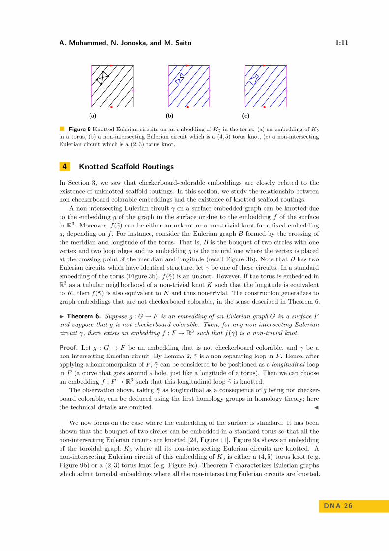
Figure 9 Knotted Eulerian circuits on an embedding of K5 in the torus. (a) an embedding of K5
in a torus, (b) a non-intersecting Eulerian circuit which is a (4, 5) torus knot, (c) a non-intersectingEulerian circuit which is a (2, 3) torus knot.
4 Knotted Scaffold Routings
In Section 3, we saw that checkerboard-colorable embeddings are closely related to theexistence of unknotted scaffold routings. In this section, we study the relationship betweennon-checkerboard colorable embeddings and the existence of knotted scaffold routings.
A non-intersecting Eulerian circuit γ on a surface-embedded graph can be knotted dueto the embedding g of the graph in the surface or due to the embedding f of the surfacein R3. Moreover, f(γ) can be either an unknot or a non-trivial knot for a fixed embeddingg, depending on f . For instance, consider the Eulerian graph B formed by the crossing ofthe meridian and longitude of the torus. That is, B is the bouquet of two circles with onevertex and two loop edges and its embedding g is the natural one where the vertex is placedat the crossing point of the meridian and longitude (recall Figure 3b). Note that B has twoEulerian circuits which have identical structure; let γ be one of these circuits. In a standardembedding of the torus (Figure 3b), f(γ) is an unknot. However, if the torus is embedded inR3 as a tubular neighborhood of a non-trivial knot K such that the longitude is equivalentto K, then f(γ) is also equivalent to K and thus non-trivial. The construction generalizes tograph embeddings that are not checkerboard colorable, in the sense described in Theorem 6.
I Theorem 6. Suppose g : G→ F is an embedding of an Eulerian graph G in a surface Fand suppose that g is not checkerboard colorable. Then, for any non-intersecting Euleriancircuit γ, there exists an embedding f : F → R3 such that f(γ) is a non-trivial knot.
Proof. Let g : G → F be an embedding that is not checkerboard colorable, and γ be anon-intersecting Eulerian circuit. By Lemma 2, γ is a non-separating loop in F . Hence, afterapplying a homeomorphism of F , γ can be considered to be positioned as a longitudinal loopin F (a curve that goes around a hole, just like a longitude of a torus). Then we can choosean embedding f : F → R3 such that this longitudinal loop γ is knotted.
The observation above, taking γ as longitudinal as a consequence of g being not checker-board colorable, can be deduced using the first homology groups in homology theory; herethe technical details are omitted. J
We now focus on the case where the embedding of the surface is standard. It has beenshown that the bouquet of two circles can be embedded in a standard torus so that all thenon-intersecting Eulerian circuits are knotted [24, Figure 11]. Figure 9a shows an embeddingof the toroidal graph K5 where all its non-intersecting Eulerian circuits are knotted. Anon-intersecting Eulerian circuit of this embedding of K5 is either a (4, 5) torus knot (e.g.Figure 9b) or a (2, 3) torus knot (e.g. Figure 9c). Theorem 7 characterizes Eulerian graphswhich admit toroidal embeddings where all the non-intersecting Eulerian circuits are knotted.
DNA 26
1:12 The Topology of Scaffold Routings on Non-Spherical Mesh Wireframes
Theorem 7 shows the existence of embeddings of Eulerian graphs where a routing as anon-intersecting Eulerian circuit would necessitate the use of knotted scaffold strands. Italso supports the suggestion in [9] that knotted scaffolds could expand the possible set ofDNA origami meshes that can be constructed.
I Theorem 7. An Eulerian graph admits a cellular embedding in a standardly embeddedtorus where all smoothed non-intersecting Eulerian circuits are knotted if and only if it admitsa cellular embedding in a torus that is not checkerboard colorable.
Proof. ( =⇒ ) By the contrapositive, if all the embeddings of a graph in a torus arecheckerboard colorable, then by Theorem 3, each of these embeddings will contain anunknotted non-intersecting Eulerian circuit.
( ⇐= ) Let g : G → T be a cellular embedding of an Eulerian graph in a torus suchthat the embedding is not checkerboard colorable. The main idea of the proof is to useself-homeomorphisms of the torus to twist g so that each of the non-intersecting circuitsbecomes a non-trivial knot when the torus is embedded in a standard fashion in R3. This ispossible because the number of non-intersecting Eulerian circuits is finite and each smoothednon-intersecting Eulerian circuit is non-separating (Lemma 2). A concrete combination oftwists is presented next.
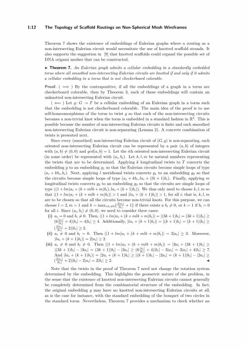
Since every (smoothed) non-intersecting Eulerian circuit of (G, g) is non-separating, eachoriented non-intersecting Eulerian circuit can be represented by a pair (a, b) of integerswith (a, b) 6= (0, 0) and gcd(a, b) = 1. Let the ith oriented non-intersecting Eulerian circuit(in some order) be represented with (ai, bi). Let k, l,m be natural numbers representingthe twists that are to be determined. Applying k longitudinal twists to T converts theembedding g to an embedding g1 so that the Eulerian circuits become simple loops of type(ai + kbi, bi). Next, applying l meridional twists converts g1 to an embedding g2 so thatthe circuits become simple loops of type (ai + kbi, lai + (lk + 1)bi). Finally, applying mlongitudinal twists converts g2 to an embedding g3 so that the circuits are simple loops oftype ((1 + lm)ai + (k+mlk+m)bi), lai + (k+ 1)bi)). We thus only need to choose k, l,m sothat |(1 + lm)ai + (k +mlk +m)bi)| > 1 and |lai + (k + 1)bi)| > 1, for all i; that is, k, l,mare to be chosen so that all the circuits become non-trivial knots. For this purpose, we canchoose l = 2,m = 1 and k = maxi:bi 6=0 2|ai|
|bi| + 1 if there exists a bi 6= 0, or k = 1 if bi = 0for all i. Since (ai, bi) 6= (0, 0), we need to consider three cases:(i) ai = 0 and bi 6= 0. Then, |(1 + lm)ai + (k+mlk+m)bi)| = |(3k+ 1)bi| = (3k+ 1)|bi| ≥
(6 |ai||bi| + 4)|bi| = 4|bi| ≥ 4. Additionally, |lai + (k + 1)bi)| = |(k + 1)bi| = (k + 1)|bi| ≥
( 2|ai||bi| + 2)|bi| ≥ 2.
(ii) ai 6= 0 and bi = 0. Then |(1 + lm)ai + (k + mlk + m)bi)| = 3|ai| ≥ 3. Moreover,|lai + (k + 1)bi)| = 2|ai| ≥ 2.
(iii) ai 6= 0 and bi 6= 0. Then |(1 + lm)ai + (k + mlk + m)bi)| = |3ai + (3k + 1)bi| ≥|(3k + 1)bi| − |3ai| = (3k + 1)|bi| − |3ai| ≥ (6 |ai|
|bi| + 4)|bi| − 3|ai| = 3|ai| + 4|bi| ≥ 7.And |lai + (k + 1)bi)| = |2ai + (k + 1)bi| ≥ |(k + 1)bi| − |2ai| = (k + 1)|bi| − |2ai| ≥( 2|ai||bi| + 2)|bi| − 2|ai| = 2|bi| ≥ 2. J
Note that the twists in the proof of Theorem 7 need not change the rotation systemdetermined by the embedding. This highlights the geometric nature of the problem, inthe sense that the existence of knotted non-intersecting Eulerian circuits cannot generallybe completely determined from the combinatorial structure of the embedding. In fact,the original embedding g may have no knotted non-intersecting Eulerian circuits at all,as is the case for instance, with the standard embedding of the bouquet of two circles inthe standard torus. Nevertheless, Theorem 7 provides a mechanism to check whether an
A. Mohammed, N. Jonoska, and M. Saito 1:13
Eulerian graph admits an embedding in a torus where all the non-intersecting Euleriancircuits are knotted, as one can algorithmically determine whether a graph admits a cellularembedding in a torus that is not checkerboard colorable. Indeed, this can be done by goingthrough the finite number of possible rotation systems of the graph, obtaining the cellularembeddings corresponding to the rotation systems via standard face-tracing algorithms intopological graph theory [12, p. 115], checking that the embedding is in a torus from thegeneralized Euler’s polyhedron formula [12, p. 27, p. 122], and then checking for checkerboardcolorability. Determining checkerboard colorability of a cellular embedding is equivalent todeciding whether the geometric dual is bipartite, which can be done through a standardbreadth-first-search algorithm.
For surfaces of genus greater than one, even checkerboard-colorable embeddings canhave knotted non-intersecting Eulerian circuits, as demonstrated by the infinite family inTheorem 8. Note that in Theorem 8, the claim is not that all non-intersecting Eulerian circuitsare knotted but that there is at least one that is knotted. The problem of characterizinggraphs which admit cellular embeddings in a standardly embedded surface Fn, n ≥ 2, so thatall non-intersecting Eulerian circuits are knotted is left for future work. Theorem 8 suggeststhat, unlike the case of the torus, checkerboard-colorable embeddings of graphs in surfaces ofgenus larger than one can possibly be routed and constructed using knotted scaffold strands.
I Theorem 8. Let Fn be an orientable closed surface of genus n that is standardly embeddedin R3.(i) For all n ≥ 2, there exist infinitely many Eulerian graphs that have checkerboard-
colorable cellular embeddings in Fn with knotted non-intersecting Eulerian circuits.(ii) For any non-trivial knot K, there exists an Eulerian graph G cellularly embedded with
a checkerboard coloring in Fn for some n ≥ 1 having K as a non-intersecting Euleriancircuit of G.
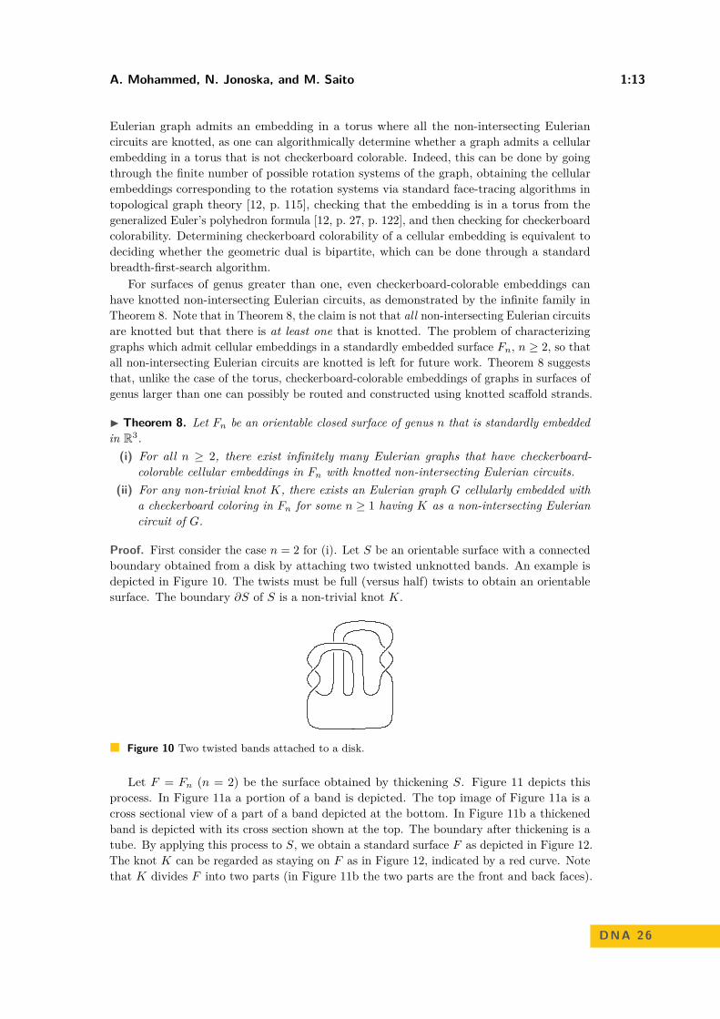
Proof. First consider the case n = 2 for (i). Let S be an orientable surface with a connectedboundary obtained from a disk by attaching two twisted unknotted bands. An example isdepicted in Figure 10. The twists must be full (versus half) twists to obtain an orientablesurface. The boundary ∂S of S is a non-trivial knot K.
Figure 10 Two twisted bands attached to a disk.
Let F = Fn (n = 2) be the surface obtained by thickening S. Figure 11 depicts thisprocess. In Figure 11a a portion of a band is depicted. The top image of Figure 11a is across sectional view of a part of a band depicted at the bottom. In Figure 11b a thickenedband is depicted with its cross section shown at the top. The boundary after thickening is atube. By applying this process to S, we obtain a standard surface F as depicted in Figure 12.The knot K can be regarded as staying on F as in Figure 12, indicated by a red curve. Notethat K divides F into two parts (in Figure 11b the two parts are the front and back faces).
DNA 26

1:14 The Topology of Scaffold Routings on Non-Spherical Mesh Wireframes
(a) (b)
Figure 11 Thickening a band (a) to a tube (b).
Next we construct a graph G cellularly embedded in F by finger moves as depicted inFigure 13. In Figure 13a, a dotted arc connects two parts of K. Push one end of K along thearc, and at the other end make it intersect in two double points as indicated in Figure 13b.After one finger move we obtain a 4-regular graph with two vertices. In Figure 14, it isshown that a finger move preserves the checkerboard colorability as in Figure 14b, and thereis a choice of a non-intersecting Eulerian circuit that is the original knot K as illustrated inFigure 14c by a blue curve. By repeating finger moves across non-cellular faces, we obtain acellularly embedded graph G with K as a non-intersecting Eulerian circuit.
Figure 12 The boundary surface after thickening contains the original knot.
This construction can be performed for any even n ∈ N. For an odd n, we add a trivialhandle to Fn−1 as indicated in Figure 15a. At this point G becomes non-cellular. To obtaina new cellularly embedded graph, we perform two finger moves as depicted in Figure 15b.The new graph retains the checkerboard colorability and the property of having K as anon-intersecting Eulerian circuit, as desired. The construction allows for infinitely many suchgraphs, for example by performing additional finger moves, or by choosing different arcs forfinger moves. This completes the proof of (i).
(a) (b)
Figure 13 A finger move (b) along a dotted arc (a).
(ii) It is known that any knot K can be realized as the boundary of an orientable surfaceS, such that a thickened S is a standard handlebody. Hence a similar argument applies. J

A. Mohammed, N. Jonoska, and M. Saito 1:15
(A) (B) (C)(a)(A) (B) (C)(b)(A) (B) (C)(c)
Figure 14 A checkerboard coloring before (a) and after a finger move (b). A choice of non-intersecting Eulerian circuit after a finger move (c).
(a) (b)
Figure 15 A handle added to make the genus odd (a) and finger moves to make the embeddingcellular (b).
5 Conclusion
Eulerian circuits are emerging as broadly applicable model of strand routings in biomoleculartechnology [4, 5, 20, 21, 32]. For circular strands, the knot type of the strand routing inthe design must conform to the knot type of the strand in solution. Herein, we studied theknottedness of strand routings modelled by non-intersecting Eulerian circuits of Euleriangraphs embedded in surfaces.
We showed a strong connection between checkerboard-colorable graph embeddings insurfaces and the knottedness of non-intersecting Eulerian circuits. We extended the resultof [24] by showing that all non-intersecting Eulerian circuits are unknotted for checkerboard-colorable torus graphs (Theorem 3). Thus, checkerboard-colorable torus graphs can berouted (as non-intersecting Eulerian circuits) using unknotted scaffolds but they cannotbe routed using knotted ones. For checkerboard-colorable embeddings in surfaces of genusgreater than one, we showed that there is at least one unknotted non-intersecting Euleriancircuit (Theorem 5). Thus, all checkerboard-colorable graph embeddings can be routedusing unknotted scaffold strands. We proved that checkerboard-colorable embedded graphsin surfaces of genus greater than one can have knotted Eulerian circuits (Theorem 8) andhence knotted scaffolds can potentially be used to construct checkerboard colorable graphembeddings in non-toroidal (and non-spherical) surfaces. For torus graphs, we characterizedEulerian graphs which admit an embedding in a standard torus where all non-intersectingEulerian circuits are knotted. These are precisely the Eulerian graphs which admit embeddingsin a torus that are not checkerboard colorable (Theorem 7). This shows the existence ofEulerian graphs embedded in surfaces that require knotted scaffolds for construction. Theresults presented can suggest, for instance, reconditioning of graphs to meet checkerboardcolorability so that unknotted scaffold routings can potentially be found. In general, knottheory of non-intersecting Eulerian circuits is also of theoretical interest, as suggested in [24].
We note that, although the problem was motivated by DNA-origami scaffold routings, theresults presented could be applied for any routing of a circular strand that can be modelledas a non-intersecting circuit in a surface-embedded graph. This is because a circuit in a
DNA 26

1:16 The Topology of Scaffold Routings on Non-Spherical Mesh Wireframes
graph can be considered as an Eulerian circuit of a subgraph. The study of surface-embeddedgraphs significantly expands the systematic ways of designing nanostructures, and the studyof the topology of circuits on such graphs can be a useful guide in the design of topologicallycomplex 3D nanostructures.
References1 Jaromir Abrham and Anton Kotzig. Construction of planar Eulerian multigraphs. In Proc.
Tenth Southeastern Conf. Comb., Graph Theory, and Computing, pages 123–130, 1979.2 Leonard M. Adleman. Molecular computation of solutions to combinatorial problems. Science,
266(5187):1021–1024, 1994. doi:10.1126/SCIENCE.7973651.3 Mark A. Armstrong. Basic Topology. Springer New York, 1983.4 Erik Benson, Abdulmelik Mohammed, Alessandro Bosco, Ana I. Teixeira, Pekka Orponen,
and Björn Högberg. Computer-aided production of scaffolded DNA nanostructures fromflat sheet meshes. Angewandte Chemie International Edition, 55(31):8869–8872, 2016. doi:10.1002/anie.201602446.
5 Erik Benson, Abdulmelik Mohammed, Johan Gardell, Sergej Masich, Eugen Czeizler, PekkaOrponen, and Björn Högberg. DNA rendering of polyhedral meshes at the nanoscale. Nature,523(7561):441–444, 2015. doi:10.1038/nature14586.
6 Samuel W. Bent and Udi Manber. On non-intersecting Eulerian circuits. Discrete AppliedMathematics, 18(1):87–94, 1987. doi:10.1016/0166-218X(87)90045-X.
7 Dorothy Buck, Egor Dolzhenko, Nataša Jonoska, Masahico Saito, and Karin Valencia. Genusranges of 4-regular rigid vertex graphs. Electronic Journal of Combinatorics, 22(3):P3.43,2015.
8 Junghuei Chen and Nadrian C. Seeman. Synthesis from DNA of a molecule with the connectivityof a cube. Nature, 350(6319):631–633, 1991. doi:10.1038/350631a0.
9 Joanna A. Ellis-Monaghan, Greta Pangborn, Nadrian C. Seeman, Sam Blakeley, Conor Disher,Mary Falcigno, Brianna Healy, Ada Morse, Bharti Singh, and Melissa Westland. Designtools for reporter strands and DNA origami scaffold strands. Theoretical Computer Science,671:69–78, 2017. doi:10.1016/j.tcs.2016.10.007.
10 Herbert Fleischner. Eulerian Graphs and Related Topics. Part 1, Volume 1, volume 45 ofAnnals of Discrete Mathematics. North-Holland Publishing Co., Amsterdam, 1990.
11 R. P. Goodman, I. A. T. Schaap, C. F. Tardin, C. M. Erben, R. M. Berry, C. F. Schmidt,and A. J. Turberfield. Rapid chiral assembly of rigid DNA building blocks for molecularnanofabrication. Science, 310(5754):1661–1665, 2005. doi:10.1126/science.1120367.
12 Jonathan L. Gross and Thomas W. Tucker. Topological Graph Theory. Dover Publications,INC, 2001. Dover reprint, original published in 1987.
13 Yu He, Tao Ye, Min Su, Chuan Zhang, Alexander E. Ribbe, Wen Jiang, and ChengdeMao. Hierarchical self-assembly of DNA into symmetric supramolecular polyhedra. Nature,452(7184):198–201, 2008. doi:10.1038/nature06597.
14 Ryosuke Iinuma, Yonggang Ke, Ralf Jungmann, Thomas Schlichthaerle, Johannes B. Woehr-stein, and Peng Yin. Polyhedra self-assembled from DNA tripods and characterized with 3DDNA-PAINT. Science, 344(6179):65–69, 2014. doi:10.1126/science.1250944.
15 Nataša Jonoska, Stephen A. Karl, and Masahico Saito. Creating 3-dimensional graph structureswith DNA. In Harvey Rubin and David H. Wood, editors, DNA Based Computers III, volume 48of DIMACS Series in Discrete Mathematics and Theoretical Computer Science, pages 123–136.AMS and DIMACS, 1999.
16 Nataša Jonoska and Masahico Saito. Boundary components of thickened graphs. In NatašaJonoska and Nadrian C. Seeman, editors, 7th International Workshop on DNA-Based Com-puters, volume 2340 of Lecture Notes in Computer Science, pages 70–81. Springer, 2001.doi:10.1007/3-540-48017-X_7.

A. Mohammed, N. Jonoska, and M. Saito 1:17
17 Hyungmin Jun, Tyson R. Shepherd, Kaiming Zhang, William P. Bricker, Shanshan Li, WahChiu, and Mark Bathe. Automated sequence design of 3D polyhedral wireframe DNA origamiwith honeycomb edges. ACS Nano, 13(2):2083–2093, 2019. doi:10.1021/acsnano.8b08671.
18 Hyungmin Jun, Xiao Wang, William P. Bricker, and Mark Bathe. Automated sequence designof 2D wireframe DNA origami with honeycomb edges. Nature Communications, 10(5419):1–9,2019. doi:10.1038/s41467-019-13457-y.
19 Hyungmin Jun, Fei Zhang, Tyson Shepherd, Sakul Ratanalert, Xiaodong Qi, Hao Yan, andMark Bathe. Autonomously designed free-form 2D DNA origami. Science Advances, 5(1),2019. doi:10.1126/sciadv.aav0655.
20 Vid Kočar, John S. Schreck, Slavko Čeru, Helena Gradišar, Nino Bašić, Tomaž Pisanski,Jonathan P. K. Doye, and Roman Jerala. Design principles for rapid folding of knotted DNAnanostructures. Nature Communications, 7:10803, 2016. doi:10.1038/ncomms10803.
21 Ajasja Ljubetič, Fabio Lapenta, Helena Gradišar, Igor Drobnak, Jana Aupič, Žiga Strmšek,Duško Lainšček, Iva Hafner-Bratkovič, Andreja Majerle, Nuša Krivec, Mojca Benčina, TomažPisanski, Tanja Ćirković Veličković, Adam Round, José María Carazo, Roberto Melero, andRoman Jerala. Design of coiled-coil protein-origami cages that self-assemble in vitro and invivo. Nature Biotechnology, 35(11):1094–1101, 2017. doi:10.1038/nbt.3994.
22 Abdulmelik Mohammed. Algorithmic Design of Biomolecular Nanostructures. PhD thesis,Aalto University, 2018.
23 Abdulmelik Mohammed and Mustafa Hajij. Unknotted strand routings of triangulated meshes.In Robert Brijder and Lulu Qian, editors, DNA Computing and Molecular Programming,volume 10467 of Lecture Notes in Computer Science, pages 46–63. Springer, 2017.
24 Ada Morse, William Adkisson, Jessica Greene, David Perry, Brenna Smith, Jo Ellis-Monaghan,and Greta Pangborn. DNA origami and unknotted A-trails in torus graphs. arXiv preprintarXiv:1703.03799, 2017. arXiv:/arxiv.org/pdf/1703.03799.pdf.
25 Dale Rolfsen. Knots and Links. AMS Chelsea Publishing, 2003. Reprint, original print in1976.
26 Paul W. K. Rothemund. Folding DNA to create nanoscale shapes and patterns. Nature,440(7082):297–302, 2006. doi:10.1038/nature04586.
27 Phiset Sa-Ardyen, Nataša Jonoska, and Nadrian C. Seeman. Self-assembling DNA graphs.Natural Computing, 2:427–438, 2003. doi:10.1023/B:NACO.0000006771.95566.34.
28 Nadrian C. Seeman. Nucleic-acid junctions and lattices. Journal of Theoretical Biology,99(2):237–247, 1982. doi:10.1016/0022-5193(82)90002-9.
29 Nadrian C. Seeman and Neville R. Kallenbach. Design of immobile nucleic acid junctions.Biophysical Journal, 44(2):201–209, 1983. doi:10.1016/S0006-3495(83)84292-1.
30 William M. Shih, Joel D. Quispe, and Gerald F. Joyce. A 1.7-kilobase single-stranded DNAthat folds into a nanoscale octahedron. Nature, 427(6975):618–621, 2004. doi:10.1038/nature02307.
31 Mu-Tsun Tsai and Douglas B. West. A new proof of 3-colorability of Eulerian triangulations.Ars Mathematica Contemporanea, 4(1):73–77, 2011.
32 Rémi Veneziano, Sakul Ratanalert, Kaiming Zhang, Fei Zhang, Hao Yan, Wah Chiu, andMark Bathe. Designer nanoscale DNA assemblies programmed from the top down. Science,352(6293):1534, 2016. doi:10.1126/science.aaf4388.
33 Gang Wu, Nataša Jonoska, and Nadrian C. Seeman. Construction of a DNA nano-object dir-ectly demonstrates computation. Biosystems, 98(2):80–84, 2009. doi:10.1016/j.biosystems.2009.07.004.
DNA 26


Simplifying Chemical Reaction NetworkImplementations with Two-Stranded DNABuilding BlocksRobert F. JohnsonCalifornia Institute of Technology, Pasadena, CA, [email protected]
Lulu QianCalifornia Institute of Technology, Pasadena, CA, USA
AbstractIn molecular programming, the Chemical Reaction Network model is often used to describe real orhypothetical systems. Often, an interesting computational task can be done with a known hypothet-ical Chemical Reaction Network, but often such networks have no known physical implementation.One of the important breakthroughs in the field was that any Chemical Reaction Network can bephysically implemented, approximately, using DNA strand displacement mechanisms. This allows usto treat the Chemical Reaction Network model as a programming language and the implementationschemes as its compiler. This also suggests that it would be useful to optimize the result of such acompilation, and in general to find effective ways to design better DNA strand displacement systems.
We discuss DNA strand displacement systems in terms of “motifs”, short sequences of elementaryDNA strand displacement reactions. We argue that describing such motifs in terms of their inputsand outputs, then building larger systems out of the abstracted motifs, can be an efficient way ofdesigning DNA strand displacement systems. We discuss four previously studied motifs in thisabstracted way, and present a new motif based on cooperative 4-way strand exchange. We then showhow Chemical Reaction Network implementations can be built out of abstracted motifs, discussingexisting implementations as well as presenting two new implementations based on 4-way strandexchange, one of which uses the new cooperative motif. The new implementations both have twodesirable properties not found in existing implementations, namely both use only at most 2-strandedDNA complexes for signal and fuel complexes and both are physically reversible. There are reasonsto believe that those properties may make them more robust and energy-efficient, but at the expenseof using more fuel complexes than existing implementation schemes.
2012 ACM Subject Classification Computer systems organization → Molecular computing
Keywords and phrases Molecular programming, DNA computing, Chemical Reaction Networks,DNA strand displacement
Digital Object Identifier 10.4230/LIPIcs.DNA.2020.2
Funding Robert F. Johnson: NSF Graduate Research Fellowship.Lulu Qian: NSF grant CCF-1908643.
Acknowledgements We would like to thank Chris Thachuk and Erik Winfree for helpful discussionson new DNA strand displacement motifs and optimization thereof.
1 Introduction
What does it mean to optimize a molecular system? One particular field in molecularprogramming is currently faced with that question. The Chemical Reaction Network (CRN)model is often used to describe systems of interacting molecules. The model can eitherdescribe real systems, to analyze their behavior and computational function, or describehypothetical systems, with known computational function but perhaps no known physical
© Robert F. Johnson and Lulu Qian;licensed under Creative Commons License CC-BY
26th International Conference on DNA Computing and Molecular Programming (DNA 26).Editors: Cody Geary and Matthew J. Patitz; Article No. 2; pp. 2:1–2:14
Leibniz International Proceedings in InformaticsSchloss Dagstuhl – Leibniz-Zentrum für Informatik, Dagstuhl Publishing, Germany

2:2 Simplifying CRN Implementations with Two-Stranded DNA Building Blocks
example. It was therefore a significant breakthrough when Soloveichik et al. showed that anyCRN, real or hypothetical, can be approximately implemented by a system of DNA stranddisplacement (DSD) mechanisms [34]. This allows the Chemical Reaction Network modelto be used as a programming language, where programs can be written in the abstract andcompiled into physical molecules. Other CRN-to-DSD implementation schemes promptlyfollowed [27, 4], each with their own strengths and weaknesses. Some have been implementedexperimentally, with variable – but mostly good – degrees of success and robustness [7, 36].Given a programming language and a concept of compiling it, one would naturally want tooptimize the result of that compilation and ask, can we do better than the best implementationschemes so far?
So what does it mean to optimize a DSD system? We focus on DNA-only (or “enzyme-free”) systems using standard toehold-mediated 3-way [45, 48] and 4-way [25, 10] stranddisplacement mechanisms. First, such DSD CRN implementations so far require “fuel species”(or “fuels”), DNA complexes that have to be synthesized by whatever method and addedto the DSD system at the start. Fuel complexes that mediate a reaction by interactingwith signal strands are often referred to as “gates”, though this is not usually formallydefined. When testing DSD circuits in the lab, fuels are chemically synthesized, annealed,and manually added to the test tube; in the hypothetical future where DSD is used inautonomous molecular devices, those devices would need some as-yet-undecided mechanismto synthesize or input fuels. Any property of the fuel species, such as length of strands,number of strands, or number of fuels, that makes them more costly to synthesize, or moredifficult to synthesize without undesired byproducts, is thus a target for optimization. Second,no physical DSD system ever does exactly what the formal DSD model says it should. Someof this is due to improbable, but not impossible, “leak reactions” not included in the formalmodel, while some is due to the aforementioned undesired byproducts or other imperfectsynthesis of the fuels [36].
In terms of robust DSD systems and their fuels, we can take a lesson from experimentswith seesaw gates [28, 40]. For a two-reactant two-product reaction, the Soloveichik et al.translation scheme uses 3-stranded fuels [34], the Cardelli scheme 4-stranded fuels [4], andthe Qian et al. scheme [27] (in the corrected version) a 5-stranded or a 7-stranded fuel. Theseesaw gates compute logic gates which are less complex than chemical reactions, but theydo so with only single strands and 2-stranded complexes [28]. Possibly because of this, theyhave been used to build larger circuits and to be robust to experimental imperfections, suchas unpurified strands [40].
For this purpose, we have been investigating implementing CRNs using only 2-strandedfuels. Simple DSD systems, such as detecting a desired sequence [5] or AND gates [16], areoften 2-stranded, in addition to the seesaw gates mentioned above. There is even a class ofhairpin-based systems that construct larger structures from single-stranded initial complexes[44], including the Hybridization Chain Reaction often used in imaging [11], and a designfor hairpin-based logic circuits [12]. However, none of these are a full Chemical ReactionNetwork implementation, or even an equivalently powerful dynamical system – while logicgates are universal for computing functions, CRNs have a dynamical behavior that logicgates in general do not.
We focus in this work on DSD systems using only 2-stranded fuels and where all mechan-isms are physically reversible. We focus on 2-stranded fuels for the robustness concerns above,as well as the theoretical question of whether 2-stranded complexes are sufficient for complexbehavior (as discussed further in [18]). We focus on physical reversiblility because it reducesthe quantity of fuel consumed by reversible reactions. Many interesting computations and

R. F. Johnson and L. Qian 2:3
... ...
(a) (b)
(c) (d)(t,s;m)
[transient]
(s,t;n) (n,m;t)*
(m,n;s)*
Figure 1 Four previously studied reversible 2-stranded DSD motifs, shown through commonexamples. (a) Toehold exchange; (b) Symmetric cooperative hybridization; (c) Asymmetric cooper-ative hybridization; (d) 4-way strand exchange, with a diagram and names used in the abstractednotation we will introduce.
dynamical behaviors require reversible reactions. For example, logically reversible operationsallow computation with arbitrarily low energy if they are implemented with physicallyreversible reactions [2, 3], such as DSD implementations of stack machines [27], Gray codecounters [9], and space-bounded computations [37]. DNA buffers [29] use reversible reactionsto maintain stable [30] and dynamical [31] spatial patterns. DNA circuits can be reset toprocess new input signals when reversible reactions are used for restoring fuel molecules inresponse to reset signals [14, 13, 12]. (Existing implementations often are or can be madephysically reversible; Qian et al. [27] demonstrate it explicitly, while simple methods to makeother existing schemes [34, 4] physically reversible is an exercise for the interested reader.)
In this work, we discuss ways of implementing CRNs using only 2-stranded fuels andwhere all mechanisms are physically reversible. We discuss four known 2-stranded DSDmotifs that can serve as building blocks for such implementations, and we present a newcooperative 4-way strand exchange motif that starts with 2-stranded complexes. We discusstwo ways of implementing general CRNs with these motifs, and tradeoffs between the twoschemes. Finally, we show how, using CRN bisimulation, these schemes can be proven correctassuming the assumptions of the formal DSD model reflect real DSD systems.
We believe that having abstract descriptions of simple motifs will help the design ofcomplex DSD systems. Whatever complex behavior is desired, it may be easier to implementby combining the simple logical operations of known motifs. To demonstrate this, wefirst discuss the 5 motifs and their behavior on an abstract level, then show how variousCRN implementations can be constructed and comprehended by combining those abstractbehaviors.
2 Two-stranded motifs
We identify five “motifs”, or simple condensed reactions, out of which we build two-strandedCRN implementations. Four of these motifs have been previously studied, while one is new.We discuss the properties of each motif in itself, while in Section 3 we will discuss how
DNA 26
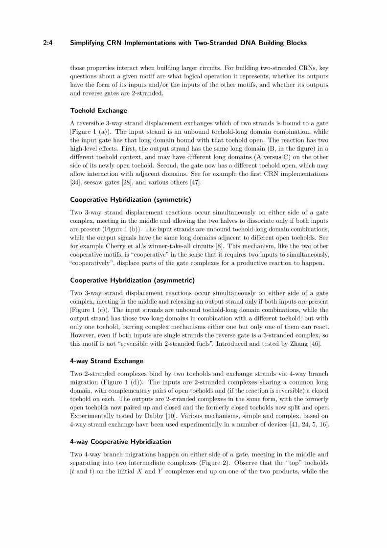
2:4 Simplifying CRN Implementations with Two-Stranded DNA Building Blocks
those properties interact when building larger circuits. For building two-stranded CRNs, keyquestions about a given motif are what logical operation it represents, whether its outputshave the form of its inputs and/or the inputs of the other motifs, and whether its outputsand reverse gates are 2-stranded.
Toehold Exchange
A reversible 3-way strand displacement exchanges which of two strands is bound to a gate(Figure 1 (a)). The input strand is an unbound toehold-long domain combination, whilethe input gate has that long domain bound with that toehold open. The reaction has twohigh-level effects. First, the output strand has the same long domain (B, in the figure) in adifferent toehold context, and may have different long domains (A versus C) on the otherside of its newly open toehold. Second, the gate now has a different toehold open, which mayallow interaction with adjacent domains. See for example the first CRN implementations[34], seesaw gates [28], and various others [47].
Cooperative Hybridization (symmetric)
Two 3-way strand displacement reactions occur simultaneously on either side of a gatecomplex, meeting in the middle and allowing the two halves to dissociate only if both inputsare present (Figure 1 (b)). The input strands are unbound toehold-long domain combinations,while the output signals have the same long domains adjacent to different open toeholds. Seefor example Cherry et al.’s winner-take-all circuits [8]. This mechanism, like the two othercooperative motifs, is “cooperative” in the sense that it requires two inputs to simultaneously,“cooperatively”, displace parts of the gate complexes for a productive reaction to happen.
Cooperative Hybridization (asymmetric)
Two 3-way strand displacement reactions occur simultaneously on either side of a gatecomplex, meeting in the middle and releasing an output strand only if both inputs are present(Figure 1 (c)). The input strands are unbound toehold-long domain combinations, while theoutput strand has those two long domains in combination with a different toehold; but withonly one toehold, barring complex mechanisms either one but only one of them can react.However, even if both inputs are single strands the reverse gate is a 3-stranded complex, sothis motif is not “reversible with 2-stranded fuels”. Introduced and tested by Zhang [46].
4-way Strand Exchange
Two 2-stranded complexes bind by two toeholds and exchange strands via 4-way branchmigration (Figure 1 (d)). The inputs are 2-stranded complexes sharing a common longdomain, with complementary pairs of open toeholds and (if the reaction is reversible) a closedtoehold on each. The outputs are 2-stranded complexes in the same form, with the formerlyopen toeholds now paired up and closed and the formerly closed toeholds now split and open.Experimentally tested by Dabby [10]. Various mechanisms, simple and complex, based on4-way strand exchange have been used experimentally in a number of devices [41, 24, 5, 16].
4-way Cooperative Hybridization
Two 4-way branch migrations happen on either side of a gate, meeting in the middle andseparating into two intermediate complexes (Figure 2). Observe that the “top” toeholds(t and t) on the initial X and Y complexes end up on one of the two products, while the

R. F. Johnson and L. Qian 2:5
“bottom” toeholds (s∗ and v∗) end up on another. That is, each of the two products carriesonly half of the information of the original reactants, and products of different instances ofthis reaction can interact in the reverse reaction. If for example the (t, t) top half of thisreaction interacted with a (v∗, s∗) bottom half from a different instance, while the (s∗, v∗)bottom half interacted with an (a, a) top half, the result would be X and Y complexes withthe same form as the original reactants but different toehold combinations. The effect of sucha quadruplet of reactions is strand exchange between one pair of complexes coupled to strandexchange between the other, simultaneously changing the open toehold combinations ondistinct long domains. This is important because affecting distinct long domains in a coupledmanner was the one thing that, under a set of additional restrictions that this mechanismsatisfies, our previous work [18] showed that uncooperative 4-way strand exchange could notdo.
While the other four mechanisms discussed have been experimentally demonstrated towork, cooperative 4-way branch migration has not yet been tested. In particular, the finaldissociation step requires 3 toeholds separated by two 4-way junctions to dissociate. Wethink this is plausible, based on Dabby’s observation that 2 toeholds separated by one 4-wayjunction can dissociate [10]; or, if this is not the case, that there is some 0 < Length(l) ≤ 6for which that dissociation is possible and reversible. It is possible that Length(l) = 0 (i.e. nothird toehold) will give the desired behavior, but from Dabby’s results, “closed” (both toeholdlengths at least 2) 4-way branch migration seems to proceed much faster than “open” 4-waybranch migration. Thus we suspect that Length(l) 6= 0, and in particular Length(l) ≥ 2,will give the desired fast and reversible reaction kinetics.
An abstraction for 4-way-based mechanisms
Common to both uncooperative and cooperative 4-way strand exchange is a basic signalcomplex: two strands, one long domain bound to its complement flanked by one boundpair of complementary toeholds and one open pair of non-complementary toeholds, as seenrepeatedly in Figures 1 (d) and 2. As both types of 4-way strand exchange transformcomplexes of this form into complexes of the same form with different domain combinations,we find an abstract description of this type of molecule useful. For example, we write themolecule with long domain X, open 3’ (end of the DNA) toehold t, open 5’ toehold s∗,and bound toehold m as X(t, s; m). Note that the semicolon distinguishes open toeholdst, s∗ available for interaction from the closed (m, m∗) toehold pair that cannot interact withother complexes, but can be opened for interaction by a reaction. When the long domain isunimportant or universal, such as a system composed entirely of uncooperative 4-way strandexchange, we omit it and write simply (t, s; m). For experimental reasons we prefer to havestrands made up of only non-∗ or only ∗ domains, and design non-∗ and ∗ domains to havedistinct sequence properties (for example, using a three-letter code [28]). Then X(t, s; m)unambiguously describes the top reactant of Figure 1 (d), with s understood to mean an opens∗ toehold. With that assumption, the top product in Figure 1 (d) would be X(m, n; s)∗,with the first toehold listed still being on the 3’ end of its strand, but now understood to meanan open m∗ toehold. Without that assumption, we might use a more general notation wherethose molecules are X(t, s∗; m) and X∗(m∗, n; s∗) respectively. The circle abstraction shownin said figures is also useful to illustrate strand exchange reactions. Each circle represents astrand with one long domain and two toeholds, where half-faded circles represent strandsmade of ∗ domains. Thin connections (both figures) represent strands bonded directly,requiring matching domains; thick connections labelled with a toehold domain (horizontalin Figure 2) represent strands connected by gate strands from a cooperative 4-way strandexchange reaction, which can be between any domains so long as the appropriate gate exists.
DNA 26

2:6 Simplifying CRN Implementations with Two-Stranded DNA Building Blocks
X(t,s;m) [signal]
[fuel]
Y(v,t;n)* [fuel]
[transients]
(m,l*,n;X:t,Y*:t*) [intermediate] (n*,l,m*;Y*:v*,X:s)
[intermediate]
Figure 2 A cooperative 4-way branch migration mechanism. Initial X and Y complexes combinewith a gate that matches their open toehold combinations, producing two 3-stranded complexeseach with one of the strands of X and one of the strands of Y . These complexes can recombinewith each other or with the corresponding products of a similar reaction, which in the latter casewill produce X and Y complexes with different toehold combinations. On the right, this reaction isshown in abstracted form. The cooperative 4-way CRN is based on groups of four of these reactions,two in the reverse of the direction shown, where in the reverse reactions each product of one forwardreaction interacts with the corresponding product of the other forward reaction. Complexes arelabeled with names in the abstract notation if applicable, and their role in the cooperative 4-wayCRN implementation scheme. “Signal” and “fuel” complexes have 2 strands as desired; stable“intermediate” complexes can have any number of strands; and “transient” complexes will quicklydecay to one side or the other of the reaction. The marking of X(t, s, m) as signal and Y (v, t, n)∗ asfuel is based on the CRN implementation scheme presented in Section 3, but in general the two canbe any combination of signal and fuel, or could be intermediates of a more complex pathway.
In Figure 2 we introduce a similar notation for the “intermediate” products of a cooperative4-way strand exchange reaction, in that case (m, l∗, n; X : t, Y ∗ : t∗) and (n∗, l, m∗; Y ∗ :v∗, X : s). Again the semicolon distinguishes the three open toeholds, listed from 5’ to 3’end, from the bound long domain-toehold pairs; each of those pairs is listed as the domainsthat appear first in 5’ to 3’ order. Thus the full reaction is
X(t, s; m) + Y (v, t, n)∗ (m, l∗, n; X : t, Y ∗ : t∗) + (n∗, l, m∗; Y ∗ : v∗, X : s)
assuming the appropriate fuel (top center), which we do not give a notation to and omitfrom the reaction, is present.
3 Chemical Reaction Network implementations
The above motifs can be combined in various ways to construct implementations of arbitraryChemical Reaction Networks. To implement arbitrary CRNs, the reaction A + B → C + D
(or A + B → C and A → B + C) is sufficient; for arbitrary reversible CRNs, the reactionA + B C (or a fortiori, A + B C + D) is sufficient [26]. From a logical perspective,“join” and “fork” operations are sufficient; the above reactions represent those logics.

R. F. Johnson and L. Qian 2:7
We take modular CRN bisimulation [19] as the definition of a “correct” CRN implement-ation scheme. Given that a scheme is correct, there are a number of other conditions thatwould be useful to satisfy for various reasons, theoretical and practical. CRN implementationstypically have signal complexes that are the primary form of a given formal species, andfuel complexes that are assumed to be always present and drive the reactions. For a CRNto have “only 2-stranded inputs”, as desired in this work, means that all signal complexesand fuel complexes are single strands or 2-stranded. We implicitly assume that we arediscussing systematic CRN implementations, where we give a template for a generic reactionand construct larger CRNs by combining independent copies of the template with differentdomain identities. In such a case we can ask how the number of toehold domains scales,i.e. whether different reactions can use the same toeholds or have to create new ones; astoeholds are limited in length by thermodynamics, a system with O(n) toeholds may be ableto implement small CRNs but a system with O(1) toeholds is better if possible. Whether ascheme requires cooperative mechanisms is worth noting. Finally, it is desirable for reversiblereactions (A + B C + D) to be implemented with physically reversible mechanisms, sothat going forward and backward multiple times does not consume fuel; to be truly reversible,the 2-stranded fuel criterion should include the reverse fuels as well. For further discussionand formal definitions of these criteria, see [18], which also contains a proof that no CRNimplementation scheme using only 4-way branch migration can satisfy all of them.
Toehold Exchange-based CRNs
Existing CRN implementations [34, 27, 4] are often based on toehold exchange mechanismswhere e.g. A + B → C is implemented by a toehold exchange reaction with A opening atoehold on the gate for a reaction involving B. These schemes can be understood in light ofthe motifs previously discussed: the property of toehold exchange that a different toeholdon the gate is opened allows join and fork logic. The property that the released strand hasa different long domain/toehold combination is used to pass signals between gates. Thesame shared-toehold logic could also be used with 4-way branch migration instead of toeholdexchange, similar to the 4-way-based AND gate [16] (although that gate itself uses a toeholdhidden in a loop rather than a toehold shared between adjacent long domains, which is aline of investigation to be explored elsewhere).
Such a shared-toehold mechanism seems to require a 3-stranded complex for the gatemolecule to achieve join logic, so it does not meet the goal of this paper, but is worthmentioning as the current state of the art. Another relevant mechanism using toeholdexchange is the seesaw gate [28], where transduction logic combines with threshold logicto check whether the total amount of signal is more than either A or B can produce byitself. This achieves join logic for macroscopic signals but cannot satisfy criteria such asCRN bisimulation for individual molecules.
3-way Cooperative CRNs
The symmetric cooperative hybridization is A + B C + D logic, if we consider the samelong domain in a different toehold context to be a different signal. Since toehold exchangereactions depend on the combination of long domain and toehold, this is valid. Thachuket al. use a combination of symmetric cooperative hybridization and toehold exchange toimplement leakless A + B → C + D reactions in exactly this manner [38, 39, 42]).
From our perspective, the only problem is that symmetric cooperative hybridization with1-stranded inputs produces 2-stranded products, and toehold exchange with a 2-strandedinput signal produces a 3-stranded reverse gate. For physically reversible reactions, this
DNA 26

2:8 Simplifying CRN Implementations with Two-Stranded DNA Building Blocks
Table 1 List of species for the 4-way O(n)-toeholds reaction A + B C + D, in the abstractednotation. Species in columns A, B, C, and D represent the given formal species. Species in columnslabeled ∅ are fuels and assumed to be always present. ai domains are toeholds specific to species A,and similarly for B, C, and D; ri domains are specific to the reaction A + B C + D; this ensuresno crosstalk with other pathways.
A ∅ B ∅(a1, a2; a3) (a2, a1; r5) (b1, b2; b3) (b2, b1; r6)(r5, a3; a1)∗ (a3, r5; a2)∗ (r6, b3; b1)∗ (b3, r6; b2)∗
(a3, r5; r2)∗ (b3, r6; r1)∗
(r2, a1; r5) (a1, r2; a3) (r1, b1; r6) (b1, r1; b3)(a1, r2; r3) (b1, r1; r4)
(r3, r5; r2)∗ (r5, r3; a1)∗ (r4, r6; r1)∗ (r6, r4; b1)∗
(r5, r3; r1)∗ (r6, r4; r2)∗
(r1, r2; r3) (r2, r1; r5) (r2, r1; r4) (r1, r2; r6)
C ∅ D ∅(c1, c2; c3) (c2, c1; r3) (d1, d2; d3) (d2, d1; r4)(c3, r3; c2)∗ (r3, c3; c1)∗ (d3, r4; d2)∗ (r4, d3; d1)∗
(r3, c3; r2)∗ (r4, d3; r1)∗
(c2, r2; r3) (r2, c2; c3) (d2, r1; r4) (r1, d2; d3)(r2, c2; r4) (r1, d2; r3)
(r3, r4; r2)∗ (r4, r3; c2)∗ (r4, r3; r1)∗ (r3, r4; d2)∗
3-stranded gate would be considered a reverse fuel, and the system would not be made withentirely 2-stranded fuels. Thus this mechanism meets all our criteria for irreversible CRNs,but not reversible CRNs.
4-way-based CRNs with O(n) toeholds
The two-toehold-mediated 4-way strand exchange mechanism effectively exchanges toeholdson a common long domain; note that while the inputs both have t and s toeholds, theoutputs have one with only t and one with only s. When a signal complex goes throughmultiple copies of this reaction with different fuels, it can turn any combination of toeholdsinto any other combination. When two signals with complementary pairs of toeholds meetin this reaction, it produces two signals with different combinations in A + B C + D
logic. So for example, we can turn (a1, a2; a3) into (r1, r2; r3) and (b1, b2; b3) into (r2, r1; r4),which will react and produce (r3, r4; r2)∗ and (r4, r3; r1)∗, which can be turned into (c1, c2; c3)and (d1, d2; d3) respectively. Thus two-toehold-mediated 4-way strand exchange alone canimplement arbitrary reversible CRNs if we allow O(n) toeholds.
A list of all species involved is given in Table 1. Note that fuels (r2, r1; r5) and (r1, r2; r6)can interact, but the products can do nothing but reverse the reaction, and the same is truefor (r4, r3; c2)∗ with (r3, r4; d2)∗.
4-way Cooperative CRNs
The cooperative 4-way strand exchange motif in Figure 2, when its products recombinewith products of a different instance of the reaction, simultaneously exchanges the toeholdcombinations on a complex with long domain X and a complex with long domain Y . If
R. F. Johnson and L. Qian 2:9
A(t, s; m) is the signal molecule for A, then simultaneously breaking the (t, s) combination onA and putting together a (u, v) combination on some long domain R is effectively convertingA(t, s; m) R(v, u; n)∗ if all other molecules involved are considered fuels. Where R isunique to the reaction A + B C + D, we can convert the four signal species from theirown long domains to the R domain, then use a two-toehold-mediated 4-way strand exchangereaction to implement the reaction itself. In contrast to the previous implementation scheme,that each reaction has a different long domain allows the toeholds (u, v, etc.) to be universal,using O(1) toeholds at the expense of requiring cooperative hybridization. In the notationused in Figure 2, this quadruplet of reactions (with the appropriate top-center fuels assumedpresent but not written) is
A(t, s; m) + R(s, u; n)∗ (m, l∗, n; A : t, R∗ : u∗) + (n∗, l, m∗ : R∗ : s∗, A : s)A(u, v; m) + R(v, t; n)∗ (m, l∗, n; A : u, R∗ : t∗) + (n∗, l, m∗ : R∗ : v∗, A : v)(m, l∗, n; A : u, R∗ : t∗) + (n∗, l, m∗ : R∗ : s∗, A : s) A(u, s; m) + R(s, t; n)∗
(m, l∗, n; A : t, R∗ : u∗) + (n∗, l, m∗ : R∗ : v∗, A : v) A(t, v; m) + R(v, u; n)∗
where A(t, s; m) and R(v, u; n)∗ are the designated meaningful complexes. The other 2-stranded complexes – A(u, v; m), A(u, s; m), A(t, v; m), R(s, u; n)∗, R(v, t; n)∗, and R(s, t; n)∗
are treated as fuels and assumed always present. If this motif works as hypothesized andwithout leak, R(v, u; n)∗ can only be produced by consuming A(t, s; m) and vice versa.
As this scheme is based on the O(n)-toehold scheme, we reuse the mechanism from Table 1.Assume all complexes in that list have long domain R, unique to the reaction A+B C +D.To the toeholds listed, add toeholds t, s, m, n, l, and let a3 = b3 = c3 = d3 = n∗, with u
and v in the above quadruplet renamed appropriately. Then use cooperative 4-way strandexchange to convert A(t, s; m) (R∗(a∗
1, a∗2; n))∗ = R(a1, a2; n∗) (the fuel will have R∗
on the “top” strand with A), B(t, s; m) R(b1, b2; n∗), C(t, s; m) R(c1, c2; n∗), andD(t, s; m) R(d1, d2; n∗). This gives a mechanism with one long domain per species, onelong domain per reaction, and a total of 19 toeholds. Because the long domains now indicatespecies/reaction identity, the toeholds can be shared between all species and reactions withoutcrosstalk.
4 Correctness of the schemes
The correctness of the schemes can be verified by CRN bisimulation, a formal definition ofcorrectness of a CRN implementation that implies several desirable properties [19]. Belowwe give an intuitive explanation of why the schemes are correct that parallels the definitionof CRN bisimulation; readers familiar with CRN bisimulation can fill in the details of theformal proof. Intuitively, CRN bisimulation consists of interpreting each DNA complex aszero or more formal species, then confirming that the behavior of the formal system and theinterpreted DSD system are the same from any initial state. That is to say, any reaction ofthe DNA complexes should be interpreted as a reaction of formal species that is either validor trivial (“anything that can happen, should”), and any reaction of the formal interpretationof a set of DNA complexes should be possible, perhaps after some trivial reactions, startingfrom that set of DNA complexes (“anything that should happen, can”).
Table 1 is effectively a proof of the correctness of the O(n)-toehold 4-way-based schemeaccording to CRN bisimulation [19]. For each A + B C + D reaction, construct a copyof this mechanism with unique ri domains, but any ai domains in common with otherreactions using the same formal species; reactions with fewer reactants or products canhave one of A, B, C, or D as a fuel; reactions with more reactants or products should
DNA 26

2:10 Simplifying CRN Implementations with Two-Stranded DNA Building Blocks
be broken into steps with at most 2 of each [26]. DNA complexes in columns labeled A,B, C, or D are interpreted as one copy of the corresponding species, while complexes incolumns labeled ∅ are fuels. Formally, fuels are assumed always present and removed fromthe enumerated implementation CRN before bisimulation verification; so for example thephysical pathway (r2, a2; r3) + (a2, r2; r5) (r5, r3; r2)∗ + (r3, r5; a2)∗ would be representedas (r2, a2; r3) (r5, r3; r2)∗, and then interpreted as the trivial reaction A A. Usingthe abstraction for 4-way strand exchange notation, the table is structured such that eachnon-fuel species can interact with the (usually two) fuel species in the same row, producingthe corresponding fuel+non-fuel pair above or below it; that the final A + B forms reactto produce the final C + D forms, while their fuels also have a spurious-but-harmlessreaction with each other; and that, given the uniqueness of the domains, no other intra-module or inter-module reactions exist. In CRN bisimulation, we say that a reactioninterpreted as, for example, A A is “trivial”, and in this case all reactions are trivialexcept (r1, r2; r3) + (r2, r1; r4) (r3, r4; r2)∗ + (r4, r3; r1)∗ which is interpreted as the desiredreaction A + B C + D. With (a1, a2; a3) etc. as the signal species, one can see that thesignal species can implement the formal reaction, and any intermediate species can turn intothe common species with the same interpretation by interacting with only fuels. Intuitivelythis is a good argument for correctness, and readers familiar with CRN bisimulation willrecognize the above as a sufficient condition for modular CRN bisimulation with respect tothe signal species as common species.
For the cooperative 4-way scheme, the same bisimulation logic applies. In the notationused in Figure 2 and Section 3, in e.g. A(t, s; m) R(a1, a2, n∗) the signal complex A(t, s; m),output complex R(a1, a2, n∗), and intermediate (m, l∗, n; A : t, R : a2) all interpreted as A,while the other three intermediates and all the fuels will each be interpreted as nothing. Fromthere the bisimulation proof follows the O(n)-toeholds case. In this case the lack of crosstalkbetween modules is assured by the distinct long domains; even if toehold combinations areidentical, different long domains will make the reaction unproductive. The remaining caveatis with the cooperative 4-way mechanism itself. We designed the system so that the toeholdsalong the cooperative reaction are always m, l, n. Thus, we assume that intermediates ofthe cooperative pathway will all have the matching m, l, n toeholds, and all three toeholdswill bind and dissociate as a unit. Whether this is actually true or not will be determinedexperimentally; if not, there may be problematic crosstalk between, for example, an (A, R1)and (A, R2) pair of long domains which leads to temporarily duplicated signals. If it is true,however, then the result of such a crosstalk will be a release of one side with the othersuspended, one of which carries the signal, and the system will be correct according tobisimulation.
5 Discussion
We discussed the use of DNA Strand Displacement to implement Chemical Reaction Networks,and the desire to create larger, more robust DSD CRN implementations. We then presented2-stranded DSD motifs which we used to build 2-stranded CRN implementations, in the hopethat they would be more robust than those which rely on 3-or-more-stranded complexes.There is some indication that 2-stranded DSD systems in general are more robust (as webriefly reviewed in the introduction), but whether these particular systems are more robustthan the current state-of-the-art CRN implementations is an open question.
We can compare Soloveichik et al.’s original CRN scheme [34, 36] (which is reasonablyrepresentative of other toehold exchange schemes), our O(n)-toehold 4-way strand exchangescheme, and our (O(1)-toehold) cooperative 4-way strand exchange scheme. While 3- and

R. F. Johnson and L. Qian 2:11
4-stranded complexes may be less robust, in other aspects the toehold exchange scheme issimpler than our two schemes: it uses one long domain per formal species, one long domain perreaction, and can be done with a single, universal toehold. To go from reactant signal speciesto product signal species in the toehold exchange scheme (as implemented experimentally[36]) takes 4 toehold exchange steps in an A + B → C + D reaction, and generalizes naturallyto n + m steps in an n-reactant m-product reaction. In contrast, while the cooperative 4-wayscheme also uses one long domain per formal species and reaction, as described above ituses 19 universal toeholds and takes 30 reactions for A + B → C + D. (By “reaction” wemean roughly one condensed reaction as described in Peppercorn [17], generalized to includetrimolecular reactions. So one toehold exchange or one 2-toehold-mediated 4-way strandexchange is one reaction, as is the cooperative 4-way strand exchange shown in Figure 2;note that using that mechanism to exchange e.g. A(t, s; m) R(a1, a2; n∗) takes 4 suchreactions.) The O(n)-toeholds scheme takes only 14 reactions for A + B → C + D, but withone universal long domain it takes 3 toeholds per species and 6 per reaction, which mayrun out of design space for large CRNs. Also, 14 reactions is still much more than 4. Thesepathways are not provably optimal; we suspect they can be reduced to less than 14 and 30,but still more than 4.
The increase in number of reactions to implement A + B → C + D may just be a costof using 2-stranded complexes. The fundamental question is, given a complex of a certainsize, how much information can it store? How can complexes meant to represent A, C,and an E from another reaction all present different enough open and bound domains thatnone can undergo a reaction meant for a different one? With 3-stranded complexes andtoehold exchange, the long domain identity and open toehold does this very efficiently. With2-stranded complexes and 4-way strand exchange, we use pairs of toehold identity to representsignal identity, which means we need extra reactions to (a) change the toehold identity onestrand at a time, and (b) ensure that intermediates of different pathways don’t try to passthrough the same toehold combination.
This question, then, connects to another work of ours. The final result of that work wasa proof that a systematic CRN implementation that satisfies certain desirable conditions,including using only 2-stranded inputs and the other conditions discussed at the beginningof Section 3, cannot be done with DSD using only 4-way branch migration [18]. The stepstaken to prove that result involve questions of what sort of transformations are possiblewith DSD reactions, and how and whether the possibility of certain transformations candepend on the features of the strands. This “dependence” is in the sense that the release ofa strand in toehold exchange “depends on” the incoming strand having the correct toeholdand long domain identities, or the way we have to structure our CRN implementations sothat production of the output species depends on the inputs having the correct toeholdidentity pairs. Thus, further exploration of that line of investigation might help answersome of the questions suggested by the mechanisms in this paper, of whether 2-strandedcomplex based CRN implementations inherently require longer pathways, and quantitativelyhow much longer. Moreover, the investigation could be expanded to include other CRNimplementations involving enzymes. For example, transcriptional circuits [20, 21], PEN-DNAtoolbox [23, 1], primer exchange reaction cascades [22], and strand-displacing polymerasesystems [35, 32, 33] all have elementary reactions that can be abstracted as motifs andare candidates for formal analysis. In these systems, it is possible to start with fewer andsimpler fuel molecules (e.g. single strands only) while more complex molecules can begenerated by DNA polymerase to carry out desired reactions. In addition to 3-way and 4-waystrand displacement with standard toeholds, other mechanisms could also be investigated,
DNA 26

2:12 Simplifying CRN Implementations with Two-Stranded DNA Building Blocks
including remote [15], associative [6], and allosteric [43] toeholds. These mechanisms mayallow further simplification of the implementations as they enrich the design space withalternative representations of signals.
It is also worth discussing how we discovered the cooperative 4-way strand exchangemotif and associated CRN implementation in the process of working out the impossibilityproof in [18]. We give an intuitive list of those conditions at the beginning of Section 3,but readers desiring a formal list of conditions should see [18]. Two of the conditions areusing only O(1) toeholds and not using cooperative mechanisms, so both the O(n) toeholdsuncooperative 4-way strand exchange based scheme and the O(1) toeholds cooperative4-way strand exchange based scheme satisfy all but one of the conditions, each failing tosatisfy a different one. Thus in some sense this paper is the positive counterpart to theprevious negative result, forming a tight upper and lower bound on the complexity of DSDimplementations of CRNs. But this pair of results also has implications for design of DSDsystems. The cooperative 4-way strand exchange motif and the process by which we cameup with it is potentially a proof of concept that, in systematically eliminating possibilitiesin DSD systems, we can find new motifs in whatever remains. How exactly this can begeneralized we do not know, but if it can be, it may make the process of designing DSDsystems faster and more systematic.
Another aspect worth mentioning is the focus on motifs before building up CRN imple-mentations. We argued that each of the 5 motifs has certain abstract behaviors, and thatlarger systems such as CRN implementations can be thought of in terms of those behaviors.When building large systems, it is much easier if one can build mid-sized building blocksout of the fundamental units, then build larger systems out of the mid-sized building blocks.Motifs take that role between fundamental DSD steps (bind, unbind, 3-way branch migration,4-way branch migration) and systems on the scale of CRN implementations. To the extentthat we were able to describe our CRN implementations in terms of the motifs rather thanin terms of the underlying DSD steps, this approach should be considered for future DSDsystem design.
References1 Nathanaël Aubert, Clément Mosca, Teruo Fujii, Masami Hagiya, and Yannick Rondelez.
Computer-assisted design for scaling up systems based on DNA reaction networks. Journal ofThe Royal Society Interface, 11(93):20131167, 2014.
2 Charles H Bennett. Logical reversibility of computation. IBM journal of Research andDevelopment, 17(6):525–532, 1973.
3 Charles H Bennett. The thermodynamics of computation—a review. International Journal ofTheoretical Physics, 21(12):905–940, 1982.
4 Luca Cardelli. Two-domain DNA strand displacement. Mathematical Structures in ComputerScience, 23(02):247–271, 2013.
5 Sherry Xi Chen, David Yu Zhang, and Georg Seelig. Conditionally fluorescent molecularprobes for detecting single base changes in double-stranded DNA. Nature Chemistry, 5(9):782,2013.
6 Xi Chen. Expanding the rule set of DNA circuitry with associative toehold activation. Journalof the American Chemical Society, 134(1):263–271, 2012.
7 Yuan-Jyue Chen, Neil Dalchau, Niranjan Srinivas, Andrew Phillips, Luca Cardelli, DavidSoloveichik, and Georg Seelig. Programmable chemical controllers made from DNA. NatureNanotechnology, 8(10):755–762, 2013.
8 Kevin M Cherry and Lulu Qian. Scaling up molecular pattern recognition with DNA-basedwinner-take-all neural networks. Nature, 559(7714):370, 2018.

R. F. Johnson and L. Qian 2:13
9 Anne Condon, Alan J Hu, Ján Maňuch, and Chris Thachuk. Less haste, less waste: onrecycling and its limits in strand displacement systems. Interface Focus, 2(4):512–521, 2012.
10 Nadine L Dabby. Synthetic molecular machines for active self-assembly: prototype algorithms,designs, and experimental study. PhD thesis, California Institute of Technology, February2013.
11 Robert M Dirks and Niles A Pierce. Triggered amplification by hybridization chain reaction.Proceedings of the National Academy of Sciences, 101(43):15275–15278, 2004.
12 Abeer Eshra, Shalin Shah, Tianqi Song, and John Reif. Renewable DNA hairpin-based logiccircuits. IEEE Transactions on Nanotechnology, 18:252–259, 2019.
13 Sudhanshu Garg, Shalin Shah, Hieu Bui, Tianqi Song, Reem Mokhtar, and John Reif. Renew-able time-responsive DNA circuits. Small, 14(33):1801470, 2018.
14 Anthony J Genot, Jonathan Bath, and Andrew J Turberfield. Reversible logic circuits madeof DNA. Journal of the American Chemical Society, 133(50):20080–20083, 2011.
15 Anthony J Genot, David Yu Zhang, Jonathan Bath, and Andrew J Turberfield. Remotetoehold: a mechanism for flexible control of DNA hybridization kinetics. Journal of theAmerican Chemical Society, 133(7):2177–2182, 2011.
16 Benjamin Groves, Yuan-Jyue Chen, Chiara Zurla, Sergii Pochekailov, Jonathan L Kirschman,Philip J Santangelo, and Georg Seelig. Computing in mammalian cells with nucleic acid strandexchange. Nature Nanotechnology, 11(3):287, 2016.
17 Casey Grun, Karthik Sarma, Brian Wolfe, Seung Woo Shin, and Erik Winfree. A domain-levelDNA strand displacement reaction enumerator allowing arbitrary non-pseudoknotted secondarystructures. CoRR, 2015. URL: http://arxiv.org/abs/1505.03738, arXiv:1505.03738.
18 Robert F. Johnson. Impossibility of sufficiently simple chemical reaction network imple-mentations in DNA strand displacement. In Ian McQuillan and Shinnosuke Seki, editors,Unconventional Computation and Natural Computation, pages 136–149. Springer InternationalPublishing, 2019. doi:10.1007/978-3-030-19311-9_12.
19 Robert F Johnson, Qing Dong, and Erik Winfree. Verifying chemical reaction networkimplementations: A bisimulation approach. Theoretical Computer Science, 2018. doi:10.1016/j.tcs.2018.01.002.
20 Jongmin Kim, John Hopfield, and Erik Winfree. Neural network computation by in vitrotranscriptional circuits. In Advances in Neural Information Processing systems, pages 681–688,2005.
21 Jongmin Kim and Erik Winfree. Synthetic in vitro transcriptional oscillators. MolecularSystems Biology, 7(1):465, 2011.
22 Jocelyn Y Kishi, Thomas E Schaus, Nikhil Gopalkrishnan, Feng Xuan, and Peng Yin. Pro-grammable autonomous synthesis of single-stranded DNA. Nature Chemistry, 10(2):155,2018.
23 Kevin Montagne, Raphael Plasson, Yasuyuki Sakai, Teruo Fujii, and Yannick Rondelez.Programming an in vitro DNA oscillator using a molecular networking strategy. MolecularSystems Biology, 7(1):466, 2011.
24 Richard A Muscat, Jonathan Bath, and Andrew J Turberfield. A programmable molecularrobot. Nano letters, 11(3):982–987, 2011.
25 Igor G Panyutin and Peggy Hsieh. The kinetics of spontaneous DNA branch migration.Proceedings of the National Academy of Sciences, 91(6):2021–2025, 1994.
26 Tomislav Plesa. Stochastic approximation of high-molecular by bi-molecular reactions. arXivpreprint arXiv:1811.02766, 2018.
27 Lulu Qian, David Soloveichik, and Erik Winfree. Efficient Turing-universal computationwith DNA polymers. In Yasubumi Sakakibara and Yongli Mi, editors, DNA Computing andMolecular Programming, volume 6518 of Lecture Notes in Computer Science, pages 123–140.Springer, 2011.
28 Lulu Qian and Erik Winfree. Scaling up digital circuit computation with DNA stranddisplacement cascades. Science, 332(6034):1196–1201, 2011.
DNA 26

2:14 Simplifying CRN Implementations with Two-Stranded DNA Building Blocks
29 Dominic Scalise, Nisita Dutta, and Rebecca Schulman. DNA strand buffers. Journal of theAmerican Chemical Society, 140(38):12069–12076, 2018.
30 Dominic Scalise and Rebecca Schulman. Designing modular reaction-diffusion programs forcomplex pattern formation. Technology, 2(01):55–66, 2014.
31 Dominic Scalise and Rebecca Schulman. Emulating cellular automata in chemical reaction-diffusion networks. Natural Computing, 15(2):197–214, 2016.
32 Shalin Shah, Tianqi Song, Xin Song, Ming Yang, and John Reif. Implementing arbitraryCRNs using strand displacing polymerase. In International Conference on DNA Computingand Molecular Programming, pages 21–36. Springer, 2019.
33 Shalin Shah, Jasmine Wee, Tianqi Song, Luis Ceze, Karin Strauss, Yuan-Jyue Chen, and JohnReif. Using strand displacing polymerase to program chemical reaction networks. Journal ofthe American Chemical Society, 2020.
34 David Soloveichik, Georg Seelig, and Erik Winfree. DNA as a universal substrate for chemicalkinetics. Proceedings of the National Academy of Sciences, 107(12):5393–5398, 2010.
35 Tianqi Song, Abeer Eshra, Shalin Shah, Hieu Bui, Daniel Fu, Ming Yang, Reem Mokhtar,and John Reif. Fast and compact DNA logic circuits based on single-stranded gates usingstrand-displacing polymerase. Nature Nanotechnology, 14(11):1075–1081, 2019.
36 Niranjan Srinivas, James Parkin, Georg Seelig, Erik Winfree, and David Soloveichik. Enzyme-free nucleic acid dynamical systems. Science, 358:doi:10.1126/science.aal2052, 2017.
37 Chris Thachuk and Anne Condon. Space and energy efficient computation with DNA stranddisplacement systems. In International Workshop on DNA-Based Computers, pages 135–149.Springer, 2012.
38 Chris Thachuk and Erik Winfree. A fast, robust, and reconfigurable molecular circuitbreadboard. 15th Annual Conference on Foundations of Nanoscience, invited talk, 2018.URL: https://thachuk.com/talk/2018-fnano-invited/2018-FNANO-invited.pdf.
39 Chris Thachuk, Erik Winfree, and David Soloveichik. Leakless DNA strand displacement sys-tems. In Andrew Phillips and Peng Yin, editors, DNA Computing and Molecular Programming,volume 9211 of Lecture Notes in Computer Science, pages 133–153. Springer, 2015.
40 Anupama J Thubagere, Chris Thachuk, Joseph Berleant, Robert F Johnson, Diana A Ardelean,Kevin M Cherry, and Lulu Qian. Compiler-aided systematic construction of large-scale DNAstrand displacement circuits using unpurified components. Nature Communications, 8:14373,2017.
41 Suvir Venkataraman, Robert M Dirks, Paul WK Rothemund, Erik Winfree, and Niles A Pierce.An autonomous polymerization motor powered by DNA hybridization. Nature Nanotechnology,2(8):490, 2007.
42 Boya Wang, Chris Thachuk, Andrew D Ellington, Erik Winfree, and David Soloveichik.Effective design principles for leakless strand displacement systems. Proceedings of the NationalAcademy of Sciences, 115(52):E12182–E12191, 2018.
43 Xiaolong Yang, Yanan Tang, Sarah M Traynor, and Feng Li. Regulation of DNA stranddisplacement using an allosteric DNA toehold. Journal of the American Chemical Society,138(42):14076–14082, 2016.
44 Peng Yin, Harry MT Choi, Colby R Calvert, and Niles A Pierce. Programming biomolecularself-assembly pathways. Nature, 451(7176):318–322, 2008.
45 Bernard Yurke and Allen P Mills. Using DNA to power nanostructures. Genetic Programmingand Evolvable Machines, 4(2):111–122, 2003.
46 David Yu Zhang. Cooperative hybridization of oligonucleotides. Journal of the AmericanChemical Society, 133(4):1077–1086, 2010.
47 David Yu Zhang and Georg Seelig. Dynamic DNA nanotechnology using strand-displacementreactions. Nature Chemistry, 3(2):103–113, 2011.
48 David Yu Zhang and Erik Winfree. Control of DNA strand displacement kinetics using toeholdexchange. Journal of the American Chemical Society, 131(47):17303–17314, 2009.
Composable Computation in Leaderless, DiscreteChemical Reaction NetworksHooman HashemiThe University of British Columbia, Vancouver, Canada
Ben ChuggStanford University, CA, [email protected]
Anne CondonThe University of British Columbia, Vancouver, [email protected]
AbstractWe classify the functions f : Nd → N that are stably computable by leaderless, output-obliviousdiscrete (stochastic) Chemical Reaction Networks (CRNs). CRNs that compute such functionsare systems of reactions over species that include d designated input species, whose initial countsrepresent an input x ∈ Nd, and one output species whose eventual count represents f(x). Chen etal. showed that the class of functions computable by CRNs is precisely the semilinear functions. Inoutput-oblivious CRNs, the output species is never a reactant. Output-oblivious CRNs are easilycomposable since a downstream CRN can consume the output of an upstream CRN without affectingits correctness. Severson et al. showed that output-oblivious CRNs compute exactly the subclass ofsemilinear functions that are eventually the minimum of quilt-affine functions, i.e., affine functionswith different intercepts in each of finitely many congruence classes. They call such functions theoutput-oblivious functions. A leaderless CRN can compute only superadditive functions, and so aleaderless output-oblivious CRN can compute only superadditive, output-oblivious functions. Inthis work we show that a function f : Nd → N is stably computable by a leaderless, output-obliviousCRN if and only if it is superadditive and output-oblivious.
2012 ACM Subject Classification Theory of computation → Models of computation; Theory ofcomputation → Formal languages and automata theory
Keywords and phrases Chemical Reaction Networks, Stable Function Computation, Output-Oblivi-ous, Output-Monotonic
Digital Object Identifier 10.4230/LIPIcs.DNA.2020.3
Funding Hooman Hashemi: Supported by an NSERC Discovery Grant.Ben Chugg: Supported by an NSERC Undergraduate Research Award.Anne Condon: Supported by an NSERC Discovery Grant.
Acknowledgements This work benefited greatly from conversations with Eric Severson and DavidDoty. Thanks also to David Haley and Eric Severson for help in generating the figures.
1 Introduction
Chemical Reaction Networks (CRNs) have proven to be very valuable as a programminglanguage for describing how computations can ensue when molecules react. There is now arich complexity theory of computation with the CRN model, as well as the closely relatedpopulation protocol model of distributed computing [2, 4, 7, 10, 11, 17]. This theory helpsus understand what types of computational or engineered dynamic processes are possiblewith molecules, since CRNs can be “compiled” down to DNA strand displacement systems,which in turn can be implemented with real DNA strands in a test tube [5, 15, 18, 19].
© Hooman Hashemi, Ben Chugg, and Anne Condon;licensed under Creative Commons License CC-BY
26th International Conference on DNA Computing and Molecular Programming (DNA 26).Editors: Cody Geary and Matthew J. Patitz; Article No. 3; pp. 3:1–3:18
Leibniz International Proceedings in InformaticsSchloss Dagstuhl – Leibniz-Zentrum für Informatik, Dagstuhl Publishing, Germany

3:2 Composable Leaderless CRN Computation
It is natural to ask: If CRNs C and C ′ compute functions f and f ′, respectively, canwe compose the CRNs to compute the composition f ′ f? In this paper we study thisquestion for leaderless, discrete CRNs, resolving an open question of Chugg et al. [9], Seversonet al. [16], and Chalk et al. [6]. Here we first describe the CRN model, background andmotivation for the work, and then describe our result in more detail.
We focus on discrete CRNs (also called stochastic CRNs), which are described as a finiteset of chemical reactions among abstract species. Discrete CRNs stably compute functionsf : Nd → N in the following sense. An input x = (x1, . . . , xd) ∈ Nd is represented by initialcounts of d designated molecular species. A single copy of a so-called leader molecule mayalso be present initially. Reactions of the CRN ensue, changing the species counts over time.Eventually, regardless of the order of reactions, the count of a designated output speciesY equals f(x) and does not subsequently change. See Figure 1. Here and throughout, weassume without loss of generality that the range of f is N, since functions that map Nd to Nl
for some l > 1 can be computed by first cloning l distinct copies of the inputs, and then foreach 1 ≤ i ≤ l, computing the ith output from the ith copy of the inputs.
X ′1 +X ′
1 → 2Y ′
X ′1 +X ′
2 → 2Y ′
X ′2 +X ′
2 → 2Y ′X ′′
2 → 2Y ′′X1 → X ′
1 +X ′′1
X2 → X ′2 +X ′′
2Y ′ + Y ′′ → Y
(a) (b) (c)
Figure 1 Examples of Chemical Reaction Networks (CRNs) for stable function computation.(a) A CRN C1 for f(x1, x2) = x1 + x2 + ((x1 + x2) mod 2), with inputs X ′
1, X′2 and output Y ′.
(b) A CRN C2 for f ′(x1, x2) = 2x2, with inputs X ′′1 , X
′′2 and output Y ′′. (The input X ′′
1 does notappear in the reaction.) (c) A CRN C for the function minf(x1, x2), 2x2. C converts its inputsX1, X2 to those needed by CRNs C1 and C2 of parts (a) and (b), and then computes the functionminf(x1, x2), 2x2 from the outputs of C1 and C2, demonstrating function composition. All threeCRNs are leaderless.
Exactly the semilinear predicates and functions are stably computable by discrete CRNs[2, 7]. Such functions are linear on each of a finite number of semilinear domains – subsets ofNd that are defined using ≥ or mod. See Figure 2.
Let C and C ′ be discrete CRNs that stably compute functions f : Nd → N and f ′ : N→ N.Suppose furthermore that C is output-oblivious: That is, the output species of C is not areactant of any reaction of C. This condition ensures that outputs produced by C can beconsumed as inputs by a downstream CRN, without affecting the correctness of C. Then ifthe output species of C is the input species of C ′, and there is no other species common toC and C ′, the CRN C ∪ C ′ computes f ′ f .
More generally, suppose that CRNs C1, C2, . . . , Cd′ stably compute the functions f1, f2,. . ., fd′ : Nd → N, and CRN C ′ stably computes f ′ : Nd′ → N. Suppose also that the Ci
are output-oblivious, the output of Ci is the ith input to C ′ and there is no other speciescommon to the CRNs. Then C1 ∪ C2 . . . Cd′ ∪ C ′ computes f ′(f1(x), f2(x), . . . , fd′(x)). Forexample, combining the reactions of the CRN of Figure 1 parts (a), (b) and (c) results in aCRN to compute the function f ′(x1, x2) = minf(x1, x2), 2x2.
If a function f is stably computable by an output-oblivious CRN with a leader, we say thatf is obliviously-computable. Obliviously-computable functions must be nondecreasing, becausea CRN on input x + x′ can produce f(x) Y’s (by ignoring inputs representing x′), and if Y ’sare never consumed, the stable output f(x + x′) that is eventually produced must then be atleast f(x). However, not all nondecreasing semilinear functions are obliviously-computable,the max function being an interesting counterexample. Chugg et al. [9] characterized the

H. Hashemi, B. Chugg, and A. Condon 3:3
(a) (b)
(c) (d)
Figure 2 Illustrations of quilt-affine functions with domain N2. (a) The function h(x) =x1 + x2 − ((x1 + x2) mod 2). (b) Domains of the function h of part (a). h(x) = x1 + x2 onthe domain Dom1 = x ∈ N2 | x1 + x2 = 0 (mod 2), shown in blue. Dom1 is linear since itequals α1(2, 0) + α2(0, 2) + α3(1, 1) + (0, 0) | α1, α2, α3 ∈ N. Also, h(x) = x1 + x2 − 1 onthe domain Dom2 = x ∈ N2 | x1 + x2 = 1 (mod 2), shown in red. The domain Dom2 isthe union of two linear sets, namely α1(2, 0) + α2(0, 2) + α3(1, 1) + (0, 1) | α1, α2, α3 ∈ N andα1(2, 0) +α2(0, 2) +α3(1, 1) + (1, 0) | α1, α2, α3 ∈ N. (c) The function f(x) = minh(x1, x2), 2x2.(d) Domains of the function f of part (c). f(x) = 2x2 on the domain Dom3 = x ∈ N2 | x2 +1 ≤ x1,shown in green. Dom3 is linear since it equals α1(1, 0) + α2(1, 1) + (1, 0) | α1, α2 ∈ N. Also,f(x1, x2) = h(x1, x2) on the semilinear domains Dom′
1 = Dom1 ∩ x ∈ N2 | x1 ≤ x2 andDom′
2 = Dom2 ∩ x ∈ N2 | x1 ≤ x2, shown in red and blue.
subclass of obliviously-computable functions with two inputs, i.e., functions f : N2 → N.Severson et al. [16] gave a general characterization of obliviously-computable functionsf : Nd → N, for any d; such functions are eventually the min of quilt-affine functions, definedas nondecreasing linear functions with a periodic intercept, see Figure 2. See Section 2 forformal definitions of quilt-affine and obliviously-computable functions.
The results of Chugg et al. and Severson et al. described so far concern discrete, output-oblivious CRNs with leaders. What about leaderless CRNs? Output-oblivious functionscomputed by a leaderless CRN C must be superadditive, i.e., f(x) + f(x′) ≥ f(x + x′). Thisis because on input x + x′, reactions of a leaderless CRN could be used to independentlycompute both f(x) and f(x′), resulting in f(x) + f(x′) output molecules, so this quantitymust be less than or equal to the eventual stable output, namely f(x + x′). This raises thequestion: Is the class of functions f : Nd → N that can be stably computed by leaderlessoutput-oblivious CRNs exactly the superadditive obliviously-computable functions? Seversonet al. showed that this is indeed the case when d = 1, but the more general case was left asan open problem. In this paper we show that the answer is “yes” for all d:
DNA 26
3:4 Composable Leaderless CRN Computation
I Theorem 1. Functions that are stably computable by leaderless output-oblivious CRNs areexactly the superadditive obliviously-computable functions.
Our proof of Theorem 1 has two parts. First, building on the previous work of Seversonet al. and Chugg et al., we provide in Claim 5 a new characterization of superadditive,obliviously-computable functions as the minimum of superadditive quilt-affine functionson well-ordered domains, which we define in Section 2. Then in Claim 14 we construct aleaderless, output-oblivious CRN for superadditive, obliviously-computable functions, usingthe well-ordered domain representation.
Our result has strong parallels with that of Chalk et al. [6] who studied composability offunction-computing CRNs for the continuous (also called mass-action) CRN model. In thismodel, real-valued species concentrations, rather than discrete species counts, evolve overtime, according to a finite set of reactions. Earlier, Chen et al. [8] showed that continuousCRNs can stably (i.e., regardless of actual reaction rates) compute positive-continuous,piecewise rational linear functions. Chalk et al. showed that such functions are obliviously-computable by continuous CRNs if and only if they are superadditive. However, the prooftechniques for the discrete and continuous CRN models are quite different.
2 The CRN Model and Obliviously-Computable Functions
Following a summary of useful notation, we describe Chemical Reaction Networks (CRNs),stable CRN function computation, and output-oblivious function computation. We thendescribe the result of Severson et al. [16] that characterizes the class of functions that are stablycomputable by output-oblivious CRNs with a leader, i.e., obliviously-computable functions,in terms of quilt-affine functions. Finally, we provide a new, alternative characterization ofobliviously-computable functions that is useful for our main results.
2.1 NotationWe use N to denote the set of nonnegative integers, N+ the positive integers, Z the integers, Qthe rationals, and Q≥0 the nonnegative rationals. Where d is understood, we use boldface torepresent d-dimensional vectors x ∈ Nd, and xi to denote the ith component of x, 1 ≤ i ≤ d.We write x ≤ x′ to denote that xi ≤ x′i, for all i, 1 ≤ i ≤ d, and x < x′ to denote that x ≤ x′and for some i, 1 ≤ i ≤ d, xi < x′i. For 1 ≤ i ≤ d, we let ei denote the d-dimensional unitvector (ei1, . . . , eid) in which all components are zero except that eii = 1. We denote thed-dimensional vector of all zero’s by 0.
For d, p ∈ N+, Zd/pZd denotes the additive group of Zd modulo p. Each element ofZd/pZd is a congruence class of the form n + pz | z ∈ Zd for some n ∈ Nd, and we denotethis set by n.
2.2 Chemical Reaction Networks and Stable Function ComputationA discrete Chemical Reaction Network (CRNs) is specified as a finite set Z = Z1, . . . , Zmof species, plus a finite set of R of reactions (s, t) = ((s1, . . . , sm), (t1, . . . , tm)) ∈ NZ × NZof the form∑
k:sk>0skZk →
∑k:tk>0
tkZk,
where for at least one j, sj 6= tj . The species Zk with sk > 0 are the reactants, which areconsumed, while those with tk > 0 are the products. (A species may be both a reactant andproduct of the same reaction). A configuration c ∈ Nm describes counts of species in Z, and
H. Hashemi, B. Chugg, and A. Condon 3:5
c(Z) denotes the count of species Z ∈ Z. Reaction (s, t) is applicable to configuration c ifs ≤ c, i.e., sufficiently many copies of each reactant are present. Application of the reactionto c results in the configuration c′ = c − s + t, and we write c → c′. If c0 → c1 → . . . ct
then we say that ct is reachable from c0 and call c0 → c1 → . . . ct an execution of the CRN.A CRN C to stably compute a function f : Nd → N has designated input species, say
X1, . . . , Xd, a designated output species, say Y , and may or may not have a designatedleader species, L ∈ Z \ I. Leaderless function computation on input x ∈ Nd starts from avalid initial configuration c0 = c0(x), where c0(Xi) = xi for 1 ≤ i ≤ d, and the count of anyother species is 0. CRN computation with a leader differs only in that the initial count ofthe leader species L is 1, i.e., c0(L) = 1. We say that C stably computes f if for every validinitial configuration c0 = c0(x) for some x, and for every configuration c reachable from c0,there exists a stable configuration c′ reachable from c such that f(x) = c′(Y ). Here, c′ isstable if for every c′′ ∈ Nm reachable from c′, c′(Y ) = c′′(Y ). That is, once configurationc′ is reached, the count of the output species does not change. Stable computation witha leader is defined in the same way, except that in the initial configuration the count of adesignated leader species L is 1.
Chen et al. [7] (building on related work of Angluin et al. [2, 4] on predicate computationby population protocols) showed that exactly the semilinear functions are stably computableby CRNs. A semilinear function is the union of partial affine functions on linear domains. Adomain E ⊂ Nd is linear if E =
∑z∈F αzz + o : αz ∈ N for some finite set F ⊂ Nd and
o ∈ Nd. Thus, if E1, E2, . . . , Em are linear sets, ∪mi=1Ei = Nd, and for 1 ≤ i ≤ m fi : Ei → N
is a partial affine function, then the function f : Nd → N where f(x) = fi(x) if x ∈ Ei issemilinear. Figure 2 shows examples of linear sets and semilinear functions, illustrating showthe union of linear sets can be defined using ≥ or mod. Doty and Hajiaghayi [11] showedthat leaderless CRNs also stably compute the semilinear functions.
2.3 Obliviously-Computable Functions As Quilt-Affine Functions
A CRN C is output-oblivious if no reaction consumes the output species. A function f isobliviously-computable if some output-oblivious CRN with a leader stably computes f . Asubclass of the obliviously-computable functions are the leaderless obliviously-computablefunctions, that can be stably computed by leaderless output-oblivious CRNs.
Severson et al. [16] defined a quilt-affine function h : Nd → Z to be a nondecreasingfunction that is the sum of a rational linear function and a periodic function. That is,for some ∇h ∈ Qd
≥0, called the gradient of h, some p ∈ N+, called the period, and someB : Zd/pZd → Q, called the periodic intercept,
h(x) = ∇h · x +B(x).
For example, the 2D function h(x) = x1 + x2 − ((x1 + x2) mod 2) of Figure 2 is quilt-affine,since it can be written as h(x) = (1, 1) · (x1, x2) + B(x), where B(0, 0) = B(1, 1) = 0 andB(0, 1) = B(1, 0) = −1. Severson et al. [16] proved the following result.
I Theorem 2. (Severson et al. [16]) A function f : Nd → N is obliviously-computable if andonly if it satisfies the following three properties:(i) f is nondecreasing, i.e., f(x) ≤ f(x′) for all x ≤ x′.(ii) There exist (nondecreasing) quilt-affine functions h1, . . . , hm : Nd → N and kf ∈ Nd
such that for all x ≥ kf , f(x) = minihi(x).
DNA 26

3:6 Composable Leaderless CRN Computation
(iii) All fixed-input restrictions of f are obliviously-computable. Here, a fixed-input restrictionof f is a function on d− 1 inputs defined as
f[xi→j](x) = f(x1, x2, . . . , xi−1, j, xi+1, . . . , xd),
for some 1 ≤ i ≤ d and j ∈ N.
2.4 Obliviously-Computable Functions As Well-Ordered Quilt-AffineFunctions
Here we adapt Severson et al.’s result to obtain a slightly different characterization ofobliviously-computable functions, as the union of partial quilt-affine functions over well-ordered domains sets. This result lays the foundation for the rest of the paper. Claim 4in Section 3 demonstrates that these partial quilt-affine functions may be assumed to besuperadditive which, coupled with Theorem 2, implicitly proves one direction of Theorem 1.Additionally, the well-ordered domain sets will be further refined by the CRN constructionin Section 4, enabling a quilt-affine function to be expressed simply as a piecewise affinefunction. A partial quilt-affine function is simply a quilt-affine function that is defined onlyover a subset of Nd.
Next we define well-ordered domain sets. Let w ∈ Nd be fixed and let 0 ≤ o ≤ w. Let
Domo (= Domo,w) = x ∈ Nd | x ≥ o and xi = oi if oi < wi. (1)
The sets Domo for 0 ≤ o ≤ w, are disjoint and their union is Nd. We call the set of setsDomo | 0 ≤ o ≤ w a well-ordered domain set, and we denote this set by WOw. The setsare ordered in the sense that if x ∈ Domo, x′ ∈ Domo′ and x ≤ x′ then o ≤ o′. Figure 3 (b)shows a well-ordered domain set for N2 where w = (4, 4). We will later use the followingproperty of well-ordered domains:
I Lemma 3. Let Domo and Domo′ be domains of a well-ordered set defined by w, andlet Domo′′ be the domain containing o + o′. Then for any x ∈ Domo, and x′ ∈ Domo′ ,x′′ = x + x′ ∈ Domo′′ .
Proof. Since x ∈ Domo and x′ ∈ Domo′ we have that x ≥ o and x′ ≥ o′. Additionally, sinceo + o′ ∈ Domo′′ , we have that x + x′ ≥ o + o′ ≥ o′′. So x′′ satisfies the first condition ofmembership in Domo′′ .
It remains to show that if o′′i < wi, then xi = o′′i . So suppose that o′′i < wi. Then it mustalso be the case that oi < wi and o′i < wi, that o′′i = oi + o′i, and that xi = oi and x′i = o′i.The result follows. J
A well-ordered quilt-affine function is the finite union of partial quilt-affine functions,each of which is defined on a domain of a well-ordered domain set.
B Claim 4. Any obliviously-computable function is the minimum of a finite number ofnondecreasing, well-ordered quilt-affine functions.
Proof. First, from the characterization of obliviously-computable functions of Severson etal. [16] given in Theorem 2 above, we identify a finite set of partial quilt-affine functions H,as follows. We include in H the functions h1, h2, . . . , hm, each with domain Domhi
= x ∈Nd | x ≥ kf, described in property (ii) of Theorem 2.3. Then we recursively augment H byconsidering each of the fixed-input restrictions f[xi→j] of f of part (iii) of the definition, foreach choice of j < kf,i, and adding the functions corresponding to f[xi→j] from property (ii)

H. Hashemi, B. Chugg, and A. Condon 3:7
(a) (b)
(c) (d)
Figure 3 (a) A well-ordered, superadditive function f with domain setWOw for w = (4, 4). Here,f(x, y) = h(x, y) = y− (y mod 2) on the red line and f = 2y− (y mod 2) + 2x− (x mod 2)− 8 onthe large 2 dimensional area. The red line corresponds to the domain Dom(3,4). (b) The well-ordereddomain set for the function f of part (a), with w = (4, 4). There is one 2D domain, eight 1D domains,and twelve 0D domains, i.e., points. (c) The function hwo obtained from h via the construction ofClaim 4. (d) The three domains Domh (in red), Dombig (in blue) and Domsmall (in green), for thefunction h of part (c). Here, wh = (3, 4).
of Theorem 2. There are d levels of recursion; the functions that are recursively added to Hhave at least one and up to d fixed inputs, and the remaining (non-fixed) inputs are lowerbounded by some constant. Thus, for each function h added to H, the domain of h has theform
Domh = x ∈ Nd | xi = kh,i if i ∈ Dh and xi ≥ kh,i otherwise, (2)
for some kh ∈ Nd and Dh ⊆ [1, . . . , d]. We can assume without loss of generality that allfunctions h ∈ H have the same period, since we can always take the least common multipleof the periods and redefine each h with respect to this least common multiple.
For each such h ∈ H we will construct a nondecreasing, well-ordered quilt-affine functionhwo : Nd → N such that hwo(x) = h(x) for all x ∈ Domh, and also f(x) ≤ hwo(x) for allx ∈ Nd −Domh. Then f = minh∈H hwo, and the claim follows.
We’ll use the following notation when describing hwo. Let ∇h = (λh,1, λh,2, . . . , λh,k) ∈Qd be the gradient of h, let λmax = dmaxh∈H,1≤i≤dλh,ie and let
∇max = (λmax, . . . , λmax).
DNA 26
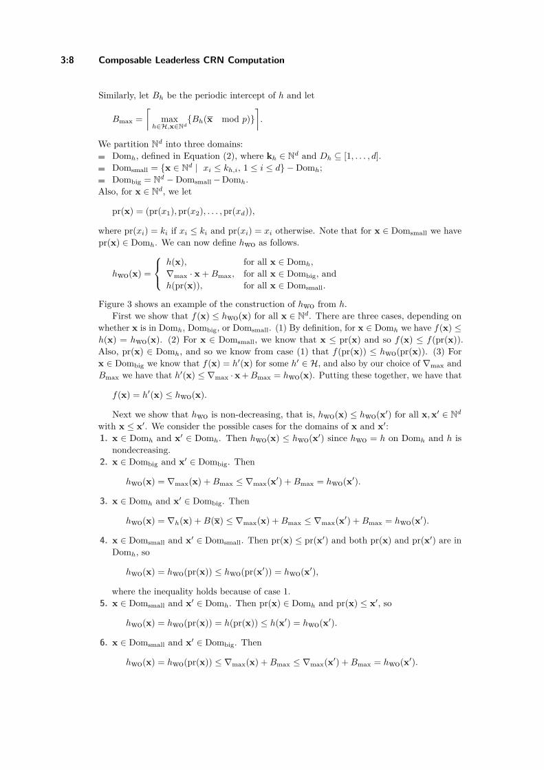
3:8 Composable Leaderless CRN Computation
Similarly, let Bh be the periodic intercept of h and let
Bmax =⌈
maxh∈H,x∈Nd
Bh(x mod p)⌉.
We partition Nd into three domains:Domh, defined in Equation (2), where kh ∈ Nd and Dh ⊆ [1, . . . , d].Domsmall = x ∈ Nd | xi ≤ kh,i, 1 ≤ i ≤ d −Domh;Dombig = Nd −Domsmall−Domh.
Also, for x ∈ Nd, we let
pr(x) = (pr(x1),pr(x2), . . . ,pr(xd)),
where pr(xi) = ki if xi ≤ ki and pr(xi) = xi otherwise. Note that for x ∈ Domsmall we havepr(x) ∈ Domh. We can now define hwo as follows.
hwo(x) =
h(x), for all x ∈ Domh,
∇max · x +Bmax, for all x ∈ Dombig, andh(pr(x)), for all x ∈ Domsmall.
Figure 3 shows an example of the construction of hwo from h.First we show that f(x) ≤ hwo(x) for all x ∈ Nd. There are three cases, depending on
whether x is in Domh, Dombig, or Domsmall. (1) By definition, for x ∈ Domh we have f(x) ≤h(x) = hwo(x). (2) For x ∈ Domsmall, we know that x ≤ pr(x) and so f(x) ≤ f(pr(x)).Also, pr(x) ∈ Domh, and so we know from case (1) that f(pr(x)) ≤ hwo(pr(x)). (3) Forx ∈ Dombig we know that f(x) = h′(x) for some h′ ∈ H, and also by our choice of ∇max andBmax we have that h′(x) ≤ ∇max ·x +Bmax = hwo(x). Putting these together, we have that
f(x) = h′(x) ≤ hwo(x).
Next we show that hwo is non-decreasing, that is, hwo(x) ≤ hwo(x′) for all x,x′ ∈ Nd
with x ≤ x′. We consider the possible cases for the domains of x and x′:1. x ∈ Domh and x′ ∈ Domh. Then hwo(x) ≤ hwo(x′) since hwo = h on Domh and h is
nondecreasing.2. x ∈ Dombig and x′ ∈ Dombig. Then
hwo(x) = ∇max(x) +Bmax ≤ ∇max(x′) +Bmax = hwo(x′).
3. x ∈ Domh and x′ ∈ Dombig. Then
hwo(x) = ∇h(x) +B(x) ≤ ∇max(x) +Bmax ≤ ∇max(x′) +Bmax = hwo(x′).
4. x ∈ Domsmall and x′ ∈ Domsmall. Then pr(x) ≤ pr(x′) and both pr(x) and pr(x′) are inDomh, so
hwo(x) = hwo(pr(x)) ≤ hwo(pr(x′)) = hwo(x′),
where the inequality holds because of case 1.5. x ∈ Domsmall and x′ ∈ Domh. Then pr(x) ∈ Domh and pr(x) ≤ x′, so
hwo(x) = hwo(pr(x)) = h(pr(x)) ≤ h(x′) = hwo(x′).
6. x ∈ Domsmall and x′ ∈ Dombig. Then
hwo(x) = hwo(pr(x)) ≤ ∇max(x) +Bmax ≤ ∇max(x′) +Bmax = hwo(x′).

H. Hashemi, B. Chugg, and A. Condon 3:9
Finally, we show that hwo is a well ordered quilt-affine function with offset wh, where wedefine wh ∈ Nd as wh,i = kh,i if i ∈ Dh and wh,i = kh,i + 1 otherwise. Consider any o ≤ wh.We need to show that hwo is quilt-affine on the domain Domo (defined in Equation (1)).There are three cases:1. If o = kh (≤ wh) then Domo = Domh. By construction, hwo = h on Domh, and h is
quilt-affine.2. If o ≤ kh but o 6= kh, then o is in Domsmall. Let o = kh − k′h, where k′h ∈ Nd. For each
x ∈ Domo we have x ∈ Domsmall, and so also pr(x) = x + k′h ∈ Domh. Therefore,
hwo(x) = hwo(pr(x))= h(pr(x))= h(x + k′h)= ∇h · (x + k′h) +B(x + k′h)= ∇h · x +∇h · k′h +B(x + k′h)= ∇h · x +B′(x),
where B′(x) = ∇h · k′h +B(x + k′h). Thus hwo is quilt-affine.3. If o ∈ Dombig, then since all x ≥ o are in Dombig, the function hwo on Domo is affine
and therefore quilt-affine with period p. C
3 Superadditive, Obliviously-Computable Functions as Quilt-AffineFunctions
In Claim 4, we showed that an obliviously-computable function f can be represented as themin of finitely many well-ordered quilt-affine functions. However, even if f is superadditive,the quilt-affine functions constructed in Claim 4 may not be superadditive. In this sectionwe strengthen that result to show in Claim 5 that if f is superadditive, then f is the min offinitely many superadditive well-ordered quilt-affine functions, thereby proving the first halfof our main result, Theorem 1.
B Claim 5. Any superadditive, obliviously-computable function is the minimum of a finitenumber of superadditive, well-ordered quilt-affine functions.
Proof. Let f : Nd → N be a superadditive, obliviously-computable function. From Claim4, we know that f = minhwo, where each of the finitely many hwo : Nd → N is a non-decreasing, well-ordered quilt-affine function. Let p be the period of the functions f and thehwo’s. Since the hwo’s may not be superadditive, we construct a superadditive, well-orderedquilt-affine function hs from each hwo, such that f = minhs.
With respect to some fixed hwo and its well-ordered domain representation, sayWOw, wefirst partition the well-ordered domains into new types of domains that we will call patches.Then we define a superadditive function hs as the union of partial affine functions on patches,such that f(x) ≤ hs(x) ≤ hwo(x) for all x ∈ Nd. Finally we further partition the patchesinto well-ordered domains to show that hs is well-ordered quilt-affine, completing the proofof the claim.
We define a patch as follows. Let n be a congruence class mod p, i.e., n = n+pz | z ∈ Zd,where n ∈ Nd. The patch defined by a corner q ∈ Nd ∩ n, a finite set of excluding pointsQ ⊂ Nd, and n is
P (q, Q,n) = x ∈ Nd ∩ n | q ≤ x and x q′,∀q′ ∈ Q.
Figure 6 of the appendix illustrates a patch, and our overall transformation from hwo to hs.
DNA 26
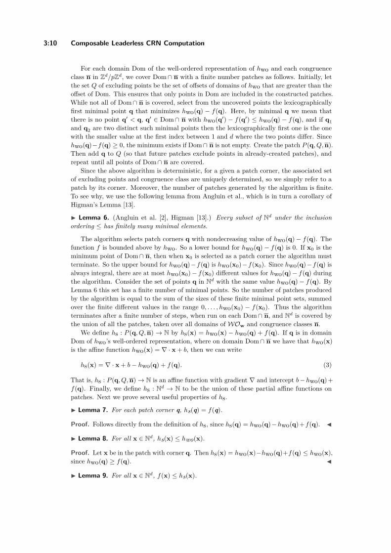
3:10 Composable Leaderless CRN Computation
For each domain Dom of the well-ordered representation of hwo and each congruenceclass n in Zd/pZd, we cover Dom∩ n with a finite number patches as follows. Initially, letthe set Q of excluding points be the set of offsets of domains of hwo that are greater than theoffset of Dom. This ensures that only points in Dom are included in the constructed patches.While not all of Dom∩ n is covered, select from the uncovered points the lexicographicallyfirst minimal point q that minimizes hwo(q) − f(q). Here, by minimal q we mean thatthere is no point q′ < q, q′ ∈ Dom∩ n with hwo(q′) − f(q′) ≤ hwo(q) − f(q), and if q1and q2 are two distinct such minimal points then the lexicographically first one is the onewith the smaller value at the first index between 1 and d where the two points differ. Sincehwo(q)−f(q) ≥ 0, the minimum exists if Dom∩ n is not empty. Create the patch P (q, Q,n).Then add q to Q (so that future patches exclude points in already-created patches), andrepeat until all points of Dom∩ n are covered.
Since the above algorithm is deterministic, for a given a patch corner, the associated setof excluding points and congruence class are uniquely determined, so we simply refer to apatch by its corner. Moreover, the number of patches generated by the algorithm is finite.To see why, we use the following lemma from Angluin et al., which is in turn a corollary ofHigman’s Lemma [13].
I Lemma 6. (Angluin et al. [2], Higman [13].) Every subset of Nd under the inclusionordering ≤ has finitely many minimal elements.
The algorithm selects patch corners q with nondecreasing value of hwo(q)− f(q). Thefunction f is bounded above by hwo. So a lower bound for hwo(q)− f(q) is 0. If x0 is theminimum point of Dom∩ n, then when x0 is selected as a patch corner the algorithm mustterminate. So the upper bound for hwo(q)−f(q) is hwo(x0)−f(x0). Since hwo(q)−f(q) isalways integral, there are at most hwo(x0)− f(x0) different values for hwo(q)− f(q) duringthe algorithm. Consider the set of points q in Nd with the same value hwo(q)− f(q). ByLemma 6 this set has a finite number of minimal points. So the number of patches producedby the algorithm is equal to the sum of the sizes of these finite minimal point sets, summedover the finite different values in the range 0, . . . , hwo(x0) − f(x0). Thus the algorithmterminates after a finite number of steps, when run on each Dom∩ n, and Nd is covered bythe union of all the patches, taken over all domains of WOw and congruence classes n.
We define hs : P (q, Q,n) → N by hs(x) = hwo(x) − hwo(q) + f(q). If q is in domainDom of hwo’s well-ordered representation, where on domain Dom∩ n we have that hwo(x)is the affine function hwo(x) = ∇ · x + b, then we can write
hs(x) = ∇ · x + b− hwo(q) + f(q). (3)
That is, hs : P (q, Q,n)→ N is an affine function with gradient ∇ and intercept b−hwo(q) +f(q). Finally, we define hs : Nd → N to be the union of these partial affine functions onpatches. Next we prove several useful properties of hs.
I Lemma 7. For each patch corner q, hs(q) = f(q).
Proof. Follows directly from the definition of hs, since hs(q) = hwo(q)−hwo(q) +f(q). J
I Lemma 8. For all x ∈ Nd, hs(x) ≤ hwo(x).
Proof. Let x be in the patch with corner q. Then hs(x) = hwo(x)−hwo(q)+f(q) ≤ hwo(x),since hwo(q) ≥ f(q). J
I Lemma 9. For all x ∈ Nd, f(x) ≤ hs(x).

H. Hashemi, B. Chugg, and A. Condon 3:11
Proof. Let x be in the patch with corner q. Then by our choice of q, hwo(q) − f(q) ≤hwo(x) − f(x). Rearranging the terms, we have that f(x) ≤ hwo(x) − hwo(q) + f(q) =hs(x). J
I Lemma 10. Let x,x′ ∈ Nd and let x ≤ x′. Then the gradient of hs on the patch containingx is less than or equal to the gradient of hs on the patch containing x′.
Proof. Suppose that x and x′ are in domains Domo and Domo′ in the well-ordered domainrepresentation of hwo. Then since x ≤ x′, the gradient of hwo on Domo is less than or equalto the gradient of hwo on Domo′ (the construction of Claim 4 satisfies this property). Byconstruction of hs in Equation (3), the gradient of hs on a patch equals the gradient of hwoin the domain containing the patch, and so the lemma follows. J
I Lemma 11. Let x,x′ ∈ Dom∩ n, for some Dom ∈ WOw and congruence class n. Supposealso that x ≤ x′. Then the intercept of hs on x is less than or equal to the intercept of hs onx′.
Proof. The stated conditions of the lemma on x and x′ imply that either x and x′ arein the same patch, or the patch containing x is constructed after the patch containing x′.The intercepts of hs on patches within Dom∩ n are nonincreasing in the order of patchconstruction. J
I Lemma 12. hs is superadditive.
Proof. Let x1 and x2 be in patches q1 and q2, respectively. Then q1 + q2 ≤ x1 + x2 andq1 + q2 and x1 + x2 are in the same congruence class. Also, by Lemma 3, the points x1 + x2and q1 + q2 lie in the same domain of hwo. Let x1 + x2 be in the patch with corner q.
On the patches with corners q1, q2, and q, let hs(x1) = ∇1 · x + b1, hs(x2) = ∇2 · x + b2,and hs(x) = ∇ · x + b, respectively. By Lemma 10, ∇1 ≤ ∇ and ∇2 ≤ ∇. Also, we have that
hs(q1) + hs(q2) = f(q1) + f(q2) (by Lemma 7)≤ f(q1 + q2) (since f is superadditive)≤ hs(q1 + q2) (by Lemma 9)≤ ∇ · (q1 + q2) + b,
where the last inequality follows by Lemmas 10 and 11. Then
hs(x1) + hs(x2) = hs(x1)− hs(q1) + hs(x2)− hs(q2) + hs(q1) + hs(q2)= ∇1 · (x1 − q1) +∇2 · (x2 − q2) + hs(q1) + hs(q2)≤ ∇ · (x1 − q1) +∇ · (x2 − q2) +∇ · (q1 + q2) + b
= ∇ · (x1 + x2) + b
= hs(x1 + x2). J
I Lemma 13. hs is well-ordered quilt-affine.
Proof. Define w′ to be the vector whose ith component w′i is maxq qi, rounded up to be 0mod p. The domain set WOw′ is a refinement of the original domain set WOw of hwo’srepresentation. Let Domo′ be one of the domains of WOw′ (where o′ ≤ w′), and letDomo′ ⊂ Domo, where Domo ∈ WOw.
Fix any congruence class n of Zd/pZd. If Domo′ ∩ n is not empty, let m be the smallestpoint in Domo′ ∩ n. Let q be the corner of the patch containing m. Note that q is in Domo.
We claim that Domo′ ∩ n is contained in the patch with corner q. This is trivially true ifDomo′ ∩ n is finite, and thus a single point. Consider the case where Domo′ is infinite. Let
DNA 26

3:12 Composable Leaderless CRN Computation
x ∈ Domo′ ∩ n and let q′ be the corner of the patch containing x. We claim that q′ ≤ m.To see why, note that if xi > mi then it must be that mi ≥ w′i and by our choice of w′,q′i ≤ mi. Otherwise, xi ≤ mi and so q′i ≤ xi ≤ mi. But then q = q′, since q is the corner ofthe patch containing m. Therefore all of Domo′ ∩ n is in the patch with corner q. It followsthat hs on domain Domo′ ∩ n is a single affine function, namely that associated with thepatch with corner q. Moreover, the gradient of this function is the gradient of the functionhwo on domain Domo ∈ WOw. Since this is true for any congruence class n, the functionhs on domain Domo′ is a quilt-affine function whose gradient is the same as that of f onDomo, completing the proof. J
From Lemmas 8 and 9, we have that f = minhs where the min is taken over a finitenumber of functions hs. Moreover, from Lemma 12, each hs is superadditive and fromLemma 13, each hs is well-ordered quilt-affine. The proof of Claim 5 follows. C
4 A Leaderless Output-Oblivious CRN for Superadditive,Obliviously-Computable Functions
Here we show the second half of our main result, Theorem 1, by constructing a leaderless,output-oblivious CRN for any superadditive, well-ordered quilt-affine function.
B Claim 14. Any superadditive, well-ordered quilt-affine function can be stably computedby a leaderless, output-oblivious CRN.
Proof. Let f : Nd → N be a superadditive, obliviously-computable function. From Claim 5,we know that f = minhs, where each of the finitely many hs is a superadditive, well-orderedquilt-affine function. Below we show that any such function has a leaderless, output-obliviousCRN, say Chs. A leaderless, output-oblivious CRN for f can then be obtained from theChs’s via the following steps: (i) for each function hs, create a unique replica Xhs,i of eachinput species Xi ; (ii) adapt Chs by replacing input species Xi by the replica Xhs,i, in everyreaction and for each i and replacing the output species Y of Chs with Yhs in every reaction;and (iii) adding the reaction
∑hs Yhs → Y , which implements the min function.
Fix any superadditive, well-ordered quilt-affine function h, and a representation of hwith well-ordered domain set WOw and period p ∈ N+. To simplify our proof we willassume without loss of generality that p > 1. Recall that there is one domain Domo in h’srepresentation for each o ≤ w. We partition these domains by taking intersections withcongruence classes mod p. For each Domo ∈ WOw and each congruence class x of Zd/pZd
such that Domo ∩ x is non-empty, let m = m(o,x) be the minimum point in the subdomainDomo ∩ x, and denote this subdomain by Dom′m. Let N be the set of all such m. By ourassumption that p > 1, it must be that all unit vectors ei are in N , 1 ≤ i ≤ d. Since h isquilt-affine with period p, we have that h(x) on Dom′m is a partial affine function, which wedenote by hm(x) = ∇m(x) + bm, where ∇m = ∇o if m = m(o,x).
Our CRN has input species X1, X2, . . . , Xd and an output species Y . We will use xto denote the vector of counts of input species consumed, and y to denote the number ofY ’s produced, during an execution of the CRN. Our CRN also has a leader species Lm form ∈ N , and a distance species Pm,i for each m ∈ N and each i ∈ 1, . . . , d. We will use#Lm and #Pm,i to denote counts of leader and distance species, during an execution of theCRN.
The leader and distances species will track how much input has been consumed byreactions. To build intuition on how this works, it may be helpful first to imagine that thereis just one leader. In this case, if the input x consumed so far is in domain Dom′m, then our

H. Hashemi, B. Chugg, and A. Condon 3:13
reactions will ensure that the leader is Lm and that for 1 ≤ i ≤ d, #Pm,i = (xi −mi)/p, i.e.,the distance of the consumed input x from m, along the ith dimension. (Since x ∈ Dom′m,xi −mi is a multiple of p.) Thus,
x = m + p∑
1≤i≤d
#Pm,i × ei.
Generalizing to the leaderless scenario, consumption of input will produce many leaders;we can imagine that the consumed input is distributed over many domains Domm. Ourreactions will ensure that a generalization of the above equality holds:
x =∑
m∈N
#Lm ×m + p∑
i∈1,...,d
#Pm,i × ei
, (4)
and we call the term on the right hand side of this invariant the input value of the CRNconfiguration. The invariant trivially holds initially since both x and the input value are 0.Our reactions will also maintain the following output invariant:
y =∑
m∈N
#Lm × h(m) +∑
i∈1,...,d
#Pm,i ×∇m,i
. (5)
We call the term on the right hand side of this invariant the output value. Initially both yand the output value are 0. We will show that once our CRN stabilizes, the output value isthe function h applied to the input value, and so these invariants ensure that y = h(x) uponstabilization.
Our CRN has three types of reactions. We next describe these, and show that eachrespects the input and output invariants. Figure 4, included in the appendix, shows anexample of a function h, a quilt-affine representation and the partitioning of the quilt-affinedomains (via intersections with congruence classes), and Figure 5, also in the appendix,illustrates part of our CRN construction for the function of Figure 4.
4.1 Input-Consuming ReactionsThese reactions consume inputs and produce leader species. There is one reaction for eachi, 1 ≤ i ≤ d:
Xi → Lei+ h(ei)× Y.
This reaction consumes input ei, and recall that by our assumption that p > 1, ei ∈ N . So,no distance species are needed to ensure that the input invariant holds. Producing h(ei) Y’sensures that the output invariant holds.
4.2 Merge ReactionsMerge reactions reduce the number of leader species, effectively electing a single leader:
Lm + Lm′ → Lm′′ + δ × Y +∑
j∈1..d
δ′jPm′′,j .
Here, m′′ is chosen such that Dom′m′′ contains m + m′. To ensure that the input invariantholds upon a merge reaction, we choose δ′j = (nj + n′j − n′′j )/p. Plugging this value into theinput invariant (4) shows that the input value is unchanged, which is necessary since no
DNA 26

3:14 Composable Leaderless CRN Computation
input is consumed. To ensure that the output invariant holds, we set δ to be equal to thechange in the output value as a result of the reaction (increase due to addition of productsminus decrease due to removal of reactants):
δ = h(m′′) + p∑
j∈1..d δ′j ×∇m′′,j − h(m)− h(m′)
= h(m + m′)− h(m)− h(m′).
In this case, δ is non-negative because f is superadditive.
4.3 Exchange ReactionsThe exchange reactions ensure that, once there is a single leader molecule, say Lm, eventuallyall of the distance species Pm′,i are such that m′ = m. Let m and m′ be in N , with m 6= m′.Let m and m′ be in the well-ordered domains of WOw with offsets o and o′, respectively.Recall that ∇m = ∇o and ∇m′ = ∇o′ . Suppose without loss of generality that o ≤ o′ (inwhich case ∇o ≤ ∇o′), and that if o = o′ then m ≤m′. Then we add the following reactions,for 1 ≤ i ≤ d:
Lm + Pm′,i → Lm + δ × Y + Pm,i.
Each exchange reaction preserves the input invariant because the input value is unchangedand no input is consumed. To ensure that the output invariant holds, we set δ to equal thechange in the output value as a result of the reaction (increase due to addition of productsminus decrease due to removal of reactants):
δ = h(m) + p∇m,i − h(m)− p∇m′,i
= p(∇m,i −∇m′,i)= p(∇o,i −∇o′,i)≥ 0, since ∇o ≥ ∇o′ .
This completes the description of the reactions of the CRN.
4.4 CorrectnessA “leader dominance” invariant that is maintained by all reactions is that for any Pm′,i
with positive count, there is also some leader Lm with positive count, such that if Domoand Domo′ are the well-ordered domains containing m and m′, respectively then o ≥ o′.The input consuming and exchange reactions trivially maintain this invariant. Consider amerge reaction with reactants Lm and Lm′ that produces Lm′′ . Suppose that m, m′, andm′′ are in the well-ordered domains with offsets Domo, Domo′ and Domo′′ , respectively.Then by Lemma 3, since Dom′m′′ contains m + m′, Domo′′ must contain o + o′. Therefore,o′′ = (o+o′)w, where we use to denote the element-wise min. So it must be that o′′ ≥ o′,and the leader dominance invariant must hold upon a merge reaction.
Next we show that the CRN stabilizes. First note that eventually all input species areconsumed by the input-consuming reactions, at which point no more leaders will be produced.Also, eventually there is exactly one leader, because of the merge reactions. At this point, theonly possible reactions are exchange reactions. Each exchange reaction reduces the numberof Pm′,i with m′ 6= m. By the leader dominance invariant, this number will eventually reachzero, at which point no more exchange reactions are possible.

H. Hashemi, B. Chugg, and A. Condon 3:15
Suppose that, once no more reactions are possible, the leader is Lm, in which case theonly distance species with count greater than zero are species Pm,i for some i. As a result,we have that
y = h(m) + p∑
i∈1..d #Pm,i ×∇m,i from the output invariant= h(m)∇np(
∑i∈1..d #Pm,i × ei + m−m)
= h(m) +∇m × (x−m) from the input invariant= h(x).
This ensures that the output is correct once the CRN has stabilized, completing the proof.C
5 Conclusion
We have classified the functions f : Nd → N which are stably computable by CRNs thatare (a) leaderless, and (b) never consume their own output. This result sheds light on thefundamental limitations of discrete CRNs. Indeed, together with previous work on CRNs withleaders [16], this has completed the classification of functions which are stably computable byoutput-oblivious CRNs – with and without leaders. Such results inform the larger questionof composability in this model of computation, and to what extent such systems can becomprised of smaller, modular components.
While composition with guaranteed correctness seems dubious for functions which arenot output-oblivious, we emphasize that there are nevertheless routes to composition with ahigh probability of correctness. Phase-clocks for example, a ubiquitous tool in populationprotocols (e.g., [3, 12, 1]), may be used to prohibit a CRN from being activated for somenumber of time steps. Kosowski and Uznański recently demonstrated how to build hierarchiesof phase clocks; these could be leveraged to construct an arbitrarily long series of CRNcompositions [14].
A question raised by our results is the extent to which the theory of discrete and continuousCRNs can be reconciled. As mentioned in the introduction, our results mirror those forcontinuous CRNs, but our techniques are quite distinct. It would be useful to know whetherand under what conditions certain statements apply to both models. Is their a theoreticalframework allowing both continuous and discrete CRNs to be studied simultaneously?
A separate question is whether CRNs which compute output-oblivious functions, but arenot themselves output-oblivious, can be augmented with reactions to make them so. ForCRNs implemented as strand displacement systems, for instance, it may be easier to addreactions than to change the underlying network entirely. Understanding the limitationsof being able to edit in this way would shed light on the possibility of building CRNsincrementally instead of requiring that the design be understood beforehand.
References1 Dan Alistarh, James Aspnes, and Rati Gelashvili. Space-optimal majority in population
protocols. In Proceedings of the Twenty-Ninth Annual ACM-SIAM Symposium on DiscreteAlgorithms, pages 2221–2239. SIAM, 2018.
2 Dana Angluin, James Aspnes, and David Eisenstat. Stably computable predicates aresemilinear. In PODC ’06: Proceedings of the twenty-fifth annual ACM symposium on Principlesof distributed computing, pages 292–299, New York, NY, USA, 2006. ACM Press. doi:10.1145/1146381.1146425.
DNA 26

3:16 Composable Leaderless CRN Computation
3 Dana Angluin, James Aspnes, and David Eisenstat. Fast computation by population protocolswith a leader. Distributed Computing, 21(3):183–199, 2008.
4 Dana Angluin, James Aspnes, David Eisenstat, and Eric Ruppert. The computational powerof population protocols. Distributed Computing, 20(4):279–304, 2007.
5 Stefan Badelt, Seung Woo Shin, Robert F. Johnson, Qing Dong, Chris Thachuk, and ErikWinfree. A general-purpose CRN-to-DSD compiler with formal verification, optimization,and simulation capabilities. In Robert Brijder and Lulu Qian, editors, DNA Computing andMolecular Programming, pages 232–248, Cham, 2017. Springer International Publishing.
6 Cameron Chalk, Niels Kornerup, Wyatt Reeves, and David Soloveichik. Composable rate-independent computation in continuous chemical reaction networks. In Milan Ceska and DavidSafránek, editors, Computational Methods in Systems Biology, pages 256–273, Cham, 2018.Springer International Publishing.
7 Ho-Lin Chen, David Doty, and David Soloveichik. Deterministic function computation withchemical reaction networks. Natural Computing, 13(4):517–534, December 2014.
8 Ho-Lin Chen, David Doty, and David Soloveichik. Rate-independent computation in continuouschemical reaction networks. In Proceedings of the 5th Conference on Innovations in TheoreticalComputer Science, ITCS 2014, pages 313–326, New York, NY, USA, 2014. Association forComputing Machinery. doi:10.1145/2554797.2554827.
9 Ben Chugg, Hooman Hashemi, and Anne Condon. Output-oblivious stochastic chemicalreaction networks. In Jiannong Cao, Faith Ellen, Luis Rodrigues, and Bernardo Ferreira,editors, 22nd International Conference on Principles of Distributed Systems, OPODIS 2018,December 17-19, 2018, Hong Kong, China, volume 125 of LIPIcs, pages 21:1–21:16. SchlossDagstuhl - Leibniz-Zentrum fuer Informatik, 2018. doi:10.4230/LIPIcs.OPODIS.2018.21.
10 Matthew Cook, David Soloveichik, Erik Winfree, and Jehoshua Bruck. Programmability ofchemical reaction networks. Algorithmic Bioprocesses, pages 543–584, 2009.
11 David Doty and Monir Hajiaghayi. Leaderless deterministic chemical reaction networks.Natural Computing, 14(2):213–223, 2015.
12 Leszek Gąsieniec and Grzegorz Staehowiak. Fast space optimal leader election in populationprotocols. In Proceedings of the Twenty-Ninth Annual ACM-SIAM Symposium on DiscreteAlgorithms, pages 2653–2667. SIAM, 2018.
13 G Higman. Ordering by divisibility in abstract algebras. Proceedings of the London Mathe-matical Society, 3(2):326–336, 1952.
14 Adrian Kosowski and Przemysław Uznański. Population protocols are fast. arXiv preprintarXiv:1802.06872, 2018.
15 Lulu Qian and Erik Winfree. Scaling up digital circuit computation with DNA stranddisplacement cascades. Science, 332(6034):1196–1201, 2011.
16 Eric E. Severson, David Haley, and David Doty. Composable computation in discrete chemicalreaction networks. In Peter Robinson and Faith Ellen, editors, Proceedings of the 2019 ACMSymposium on Principles of Distributed Computing, PODC 2019, Toronto, ON, Canada, July29 - August 2, 2019, pages 14–23. ACM, 2019. doi:10.1145/3293611.3331615.
17 David Soloveichik, Matthew Cook, Erik Winfree, and Jehoshua Bruck. Computation withfinite stochastic chemical reaction networks. Natural Computing, 7, 2008.
18 David Soloveichik, Georg Seelig, and Erik Winfree. DNA as a universal substrate for chemicalkinetics. Proceedings of the National Academy of Sciences, 107(12):5393–5398, 2010.
19 David Zhang and Georg Seelig. Dynamic DNA nanotechnology using strand-displacementreactions. Nature chemistry, 3:103–13, February 2011. doi:10.1038/nchem.957.
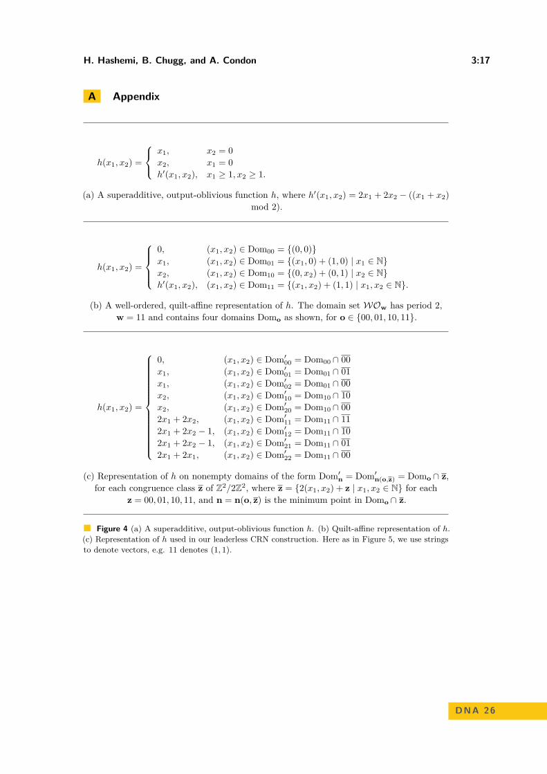
H. Hashemi, B. Chugg, and A. Condon 3:17
A Appendix
h(x1, x2) =
x1, x2 = 0x2, x1 = 0h′(x1, x2), x1 ≥ 1, x2 ≥ 1.
(a) A superadditive, output-oblivious function h, where h′(x1, x2) = 2x1 + 2x2 − ((x1 + x2)mod 2).
h(x1, x2) =
0, (x1, x2) ∈ Dom00 = (0, 0)x1, (x1, x2) ∈ Dom01 = (x1, 0) + (1, 0) | x1 ∈ Nx2, (x1, x2) ∈ Dom10 = (0, x2) + (0, 1) | x2 ∈ Nh′(x1, x2), (x1, x2) ∈ Dom11 = (x1, x2) + (1, 1) | x1, x2 ∈ N.
(b) A well-ordered, quilt-affine representation of h. The domain set WOw has period 2,w = 11 and contains four domains Domo as shown, for o ∈ 00, 01, 10, 11.
h(x1, x2) =
0, (x1, x2) ∈ Dom′00 = Dom00 ∩ 00x1, (x1, x2) ∈ Dom′01 = Dom01 ∩ 01x1, (x1, x2) ∈ Dom′02 = Dom01 ∩ 00x2, (x1, x2) ∈ Dom′10 = Dom10 ∩ 10x2, (x1, x2) ∈ Dom′20 = Dom10 ∩ 002x1 + 2x2, (x1, x2) ∈ Dom′11 = Dom11 ∩ 112x1 + 2x2 − 1, (x1, x2) ∈ Dom′12 = Dom11 ∩ 102x1 + 2x2 − 1, (x1, x2) ∈ Dom′21 = Dom11 ∩ 012x1 + 2x1, (x1, x2) ∈ Dom′22 = Dom11 ∩ 00
(c) Representation of h on nonempty domains of the form Dom′n = Dom′n(o,z) = Domo ∩ z,for each congruence class z of Z2/2Z2, where z = 2(x1, x2) + z | x1, x2 ∈ N for each
z = 00, 01, 10, 11, and n = n(o, z) is the minimum point in Domo ∩ z.
Figure 4 (a) A superadditive, output-oblivious function h. (b) Quilt-affine representation of h.(c) Representation of h used in our leaderless CRN construction. Here as in Figure 5, we use stringsto denote vectors, e.g. 11 denotes (1, 1).
DNA 26

3:18 Composable Leaderless CRN Computation
Input-consuming Sample Merge Sample ExchangeReactions Reactions (involving L01 or L11) Reactions (involving L11 or L22)
X1 → L10 + Y
X2 → L01 + Y
L01 + L10 → L11 + 2YL01 + Lx1 → Lx2, x ∈ 0, 1L01 + L21 → L22 + 2YL01 + L02 → L01 + P01,2
L01 + Lx2 → Lx1 + 2Y + Px1,2, x ∈ 1, 2
L11 + L01 → L21
L11 + L11 → L22
L11 + L21 → L12 + P21,1
L11 + L12 → L21 + P21,2
L11 + L22 → L11 + 2Y + P11,x, x ∈ 1, 2
L11 + P01,x → P11,x + 2YL11 + P10,x → P11,x + 2Y
L22 + P01,x → P22,x + 2YL22 + P10,x → P22,x + 2YL22 + P11,x → P22,x
L22 + P21,x → P22,x
L22 + P12,x → P22,x
Figure 5 Sample reactions of the leaderless, output-oblivious CRN for the function h of Figure 4,obtained from our construction of Claim 14.
(a) (b)
(c) (d)
Figure 6 (a) An output-oblivious function f(x). (b) By Claim 4, the function f of part (a)can be written as f = minhwo, where each of the finitely many functions hwo is nondecreasing,well-ordered quilt-affine. One of these functions is shown here. This function happens to be quitesimple, with period 1 and one domain, namely N2, and f = hwo on the red line shown in part (a).(c) The superadditive, obliviously-computable function hs that is derived from the function hwo ofpart (b) via the construction of Claim 5. Patch corners are shown as red dots. The function hs hasthe same gradient as hwo on each patch, but has different intercepts. (d) Each coloured region is apatch on N2 (i.e., the congruence class has period 1). These patches correspond to the corners ofpart (c).

CRNs Exposed: A Method for the SystematicExploration of Chemical Reaction NetworksMarko VasicThe University of Texas at Austin, TX, USAhttps://marko-vasic.github.io/[email protected]
David SoloveichikThe University of Texas at Austin, TX, USAhttp://users.ece.utexas.edu/~soloveichik/[email protected]
Sarfraz KhurshidThe University of Texas at Austin, TX, USAhttps://users.ece.utexas.edu/~khurshid/[email protected]
AbstractFormal methods have enabled breakthroughs in many fields, such as in hardware verification, machinelearning and biological systems. The key object of interest in systems biology, synthetic biology, andmolecular programming is chemical reaction networks (CRNs) which formalizes coupled chemicalreactions in a well-mixed solution. CRNs are pivotal for our understanding of biological regulatoryand metabolic networks, as well as for programming engineered molecular behavior. Although it isclear that small CRNs are capable of complex dynamics and computational behavior, it remainsdifficult to explore the space of CRNs in search for desired functionality. We use Alloy, a toolfor expressing structural constraints and behavior in software systems, to enumerate CRNs withdeclaratively specified properties. We show how this framework can enumerate CRNs with a varietyof structural constraints including biologically motivated catalytic networks and metabolic networks,and seesaw networks motivated by DNA nanotechnology. We also use the framework to exploreanalog function computation in rate-independent CRNs. By computing the desired output value withstoichiometry rather than with reaction rates (in the sense that X → Y + Y computes multiplicationby 2), such CRNs are completely robust to the choice of reaction rates or rate law. We find thesmallest CRNs computing the max, minmax, abs and ReLU (rectified linear unit) functions in anatural subclass of rate-independent CRNs where rate-independence follows from structural networkproperties.
2012 ACM Subject Classification Theory of computation
Keywords and phrases molecular programming, formal methods
Digital Object Identifier 10.4230/LIPIcs.DNA.2020.4
Supplementary Material We release the source code of our tool at https://github.com/marko-vasic/crnsExposed to enable others make use of it, and extend it further.
Acknowledgements This work was supported in part by NSF grants CCF-1901025 to DS andCCF-1718903 to SK.
1 Introduction
Formal methods have enabled breakthroughs in many fields, e.g., in hardware verification [15],machine learning [23, 32], and biological systems [5, 24, 29, 40, 61]. In this paper we applyformal methods to Chemical Reaction Networks (CRNs), which have been objects of intensestudy in systems and synthetic biology. CRNs are widely used in modeling biologicalregulatory networks, and essentially identical models are also widely used in ecology [60],
© Marko Vasic, David Soloveichik, and Sarfraz Khurshid;licensed under Creative Commons License CC-BY
26th International Conference on DNA Computing and Molecular Programming (DNA 26).Editors: Cody Geary and Matthew J. Patitz; Article No. 4; pp. 4:1–4:25
Leibniz International Proceedings in InformaticsSchloss Dagstuhl – Leibniz-Zentrum für Informatik, Dagstuhl Publishing, Germany

4:2 CRNs Exposed
distributed computing [2], and other fields. More recently, CRNs have been directly used asa programming language for engineering molecules obeying prescribed interaction rules viaDNA strand displacement cascades [6, 12,53,55,57].
It is clear that small CRNs can exhibit very complex behavior. Dynamical systems, e.g.,oscillatory, chaotic, and bistable systems, typically contain only a few reactions. Small CRNsalso exhibit interesting computational behavior. For example, the approximate majoritypopulation protocol studied in distributed computing [1] was later identified with a variety ofbiological networks [7]. Can we systematically explore the power of small reaction networks?
We present a method that exhaustively enumerates small CRNs in different classesthat are relevant for biology and for synthetic engineering systems. The enumeration isperformed using Alloy, a powerful tool for modeling structural constraints and behaviorin software systems using first-order logic with transitive closure [33]. The Alloy toolperforms scope-bounded analysis [35]. Given an Alloy model and a scope, i.e., a bound on theuniverse of discourse, the analyzer translates the Alloy model to a propositional satisfiability(SAT) formula and invokes an off-the-shelf SAT solver [20] to analyze the model. Alloy isused in a wide range of areas in software engineering, including software design [21, 34],analysis [19, 22, 36, 38], testing [44], and security [37]. We show how Alloy can be used toconveniently model interesting classes of CRNs for biology and bioengineering, and we usethe Alloy analyzer to search for CRNs with specific desired functionality.
As examples of the method we first focus on a number of classes: elementary, catalytic,metabolic. We say elementary reactions are CRNs with at most two reactants and products.(We allow reactions to be irreversible; reversible reactions are represented by two irreversiblereactions.) Catalytic networks are those elementary CRNs in which the reactants andproducts are not disjoint; i.e., the reaction is catalyzed by some species that is not consumedin the reaction. Catalytic networks (e.g., transcriptional, phosphorylation, etc.) regulatemany aspects of the cell’s behavior [42, 48]. In general protein-protein interactions, proteinscan catalytically modify other proteins, which in turn can be catalysts in other interactions.An important subclass of catalytic networks are metabolic networks, where the enzymes areproteins while the substrates are small molecules; these catalytic CRNs are “bipartite” in thesense that a species is either always a catalyst or never a catalyst. Autocatalytic networksare another interesting subclass of catalytic networks in which the (auto)catalyst generatesanother copy of itself. Autocatalysis is useful for exponential amplification and oscillation.
We then turn our attention to classes of CRNs especially relevant for synthetic reactionnetworks, showing how abstract molecular structure can be modeled in Alloy. In particular,we focus on DNA strand displacement cascades, which have proved to be a uniquely pro-grammable technology for cell-free DNA-only systems [64]. Strand displacement interactionscorrespond to reactions between two types of molecules: “gates” and “strands”, where thereacting strand displaces the strand previously sequestered in the gate complex. A simple,yet very scalable, class of strand displacement circuits uses a simple motif called seesawgates [13,49,50] that makes use of a reversible strand displacement reaction. We designedan Alloy model to enumerate such strand displacement reactions, showing that abstractmolecular structure can be incorporated into the Alloy modeling formalism.
In the second part of the paper, we use our enumeration framework to search for specificdesired functionality in a class of CRNs. In particular, we focus on the class of rate-independent CRNs [11]. Consider the reaction X → Y + Y , and think of the concentrationsof species X and Y as input and output respectively. This reaction computes the functionof “multiplication by 2” since in the limit of time going to infinity it produces two units ofY for every unit of X initially present. Similarly the reaction X1 + X2 → Y computes the

M. Vasic, D. Soloveichik, and S. Khurshid 4:3
A −−→ Z1 + Y
B −−→ Z2 + Y
Z1 + Z2 −−→ K
Y + K −−→ ∅
Figure 1 CRN computing Max. We think of the initial amount of A and B as inputs, and theconverging amount of Y as the output. The amount of Y eventually produced in reactions 1 and 2is the sum of the initial amounts of A and B. The amount of K eventually produced in reaction 3 isthe minimum of the initial amounts of A and B. Reaction 4 subtracts the minimum from the sum,yielding the maximum. (The 4th reaction generates waste species, which are not named.)
“minimum” function since the amount of Y eventually produced will be the minimum ofthe initial amounts of X1 and X2. Note that such computation makes no assumption onthe rate law, such as whether the reaction obeys mass-action kinetics1 or not, allowing thecomputation to be correct in a wide variety of chemical contexts. (We use the continuousCRN model where concentrations are real-valued quantities.)
A natural subclass of CRNs whose structure enforces rate independence are those thatsatisfy two constraints: feed-forward, and non-competitive.2 Intuitively, the first conditionensures that the CRN converges to a static equilibrium where no reaction can occur. Thesecond condition ensures that no matter what the rates are, the system converges to thesame static equilibrium. More precisely, we define feed-forward as follows: there exists atotal ordering on the reactions such that no reaction consumes3 a species produced by areaction later in the ordering. We define non-competitive as follows: if a species is consumedin a reaction then it cannot appear as a reactant somewhere else. Such constraints on thestructure of the network can be easily encoded in the Alloy specification. We also require eachreaction to consume at least one species (boundedness condition). We show in Appendix Athat these conditions ensure that the CRN is rate-independent.
Focusing on the class of feed-forward, non-competitive CRNs, we search for the smallestreaction networks implementing max, minmax, abs, and ReLU (rectified linear unit) functions.As an example of the kind of computation we achieve, consider the max computing CRNshown in Figure 1. This CRN was previously studied [10, 11]; our result shows that it isindeed the smallest. The maximum function serves an important role in rate-independentcomputation since together with minimum, multiplication and division by a constant itforms a complete basis set [9, 11]. The ReLU function was first introduced due to thebiological motivations explaining functioning of neurons in the brain cortex [27]. Since then,it was used with great success in the machine learning community, particularly in deeplearning [25, 41] for realizing artificial neural networks. The simplicity of its implementationsuggests that CRNs can naturally realize neural computation [58]. To our knowledge, thesmallest implementations of abs (absolute value), and minmax (a two output functioncomputing both minimum and maximum of two inputs) that we find are novel and have notbeen previously published.
1 “Mass-action” kinetics refers to the best-studied case where the reaction rate is proportional to theproduct of the concentration of the reactants.
2 Feed-forward and non-competitive conditions are sufficient for rate-independence, but are not necessary.However, most known examples of rate independent computation satisfy these conditions.
3 We say a reaction produces (resp. consumes) a species S if there is net stoichiometric gain (resp. loss) ofS. Thus a catalyst in a reaction is neither consumed nor produced.
DNA 26

4:4 CRNs Exposed
Listing 1 General Alloy model of CRNs. “−−” indicate start of a comment.module crn
abstract sig Species abstract sig Reaction reactants, products: seq Species
-- Basic semantic constraints -- for all CRNsfact AtLeastOneReactant -- each reaction has >=1 reactantall r: Reaction | some r.reactants
fact UniqueReactions -- each reaction is uniqueall disj r1, r2 : Reaction | ReactionsDifferent[r1, r2]
pred ReactionsDifferent[r1, r2: Reaction] SpeciesSeqDifferent[r1.reactants, r2.reactants]or SpeciesSeqDifferent[r1.products, r2.products]
pred SpeciesSeqDifferent[seq1, seq2: seq Species] some s : Species | #indsOf[seq1, s] != #indsOf[seq2, s]
fact ReactantsDifferentThanProducts all r: Reaction | SpeciesSeqDifferent[r.reactants, r.products]
fact AllSpeciesUsed -- each species is used in some reactionInt.(Reaction.(reactants + products)) = Species
pred ContainsAsReactant[r: Reaction, s: Species] s in Int.(r.reactants) pred ContainsAsProduct[r: Reaction, s: Species] s in Int.(r.products)
Much ongoing work explores the computational power of CRNs. Previous work showedthe implementation of numerous complex behaviors, such as mapping polynomials to chemicalreactions [51], programming logic gates [43], mapping discrete, control flow, algorithms [31],and a molecular programming language translating high-level specifications to chemicalreactions [59]. However the complexity of these reaction systems can be infeasible, asking fornovel techniques that answer what is the natural way to compute “in reactions”. To helpanswer this question we can take a different, bottom-up approach, and explore what smallCRNs naturally do. We believe that insight we get from exploring reactions will help indesign of higher-level primitives that naturally map to reactions, and will provide knowledgefor more efficient design of high-level languages.
2 Modeling CRNs in Alloy
This section describes our approach to modeling chemical reaction networks (CRNs) in Alloy.(See Appendix B for additional background on Alloy.) We first introduce a general model torepresent the broadest class of CRNs (allowing arbitrary number of reactants and products),and next show specializations of the model for different classes such as elementary, catalytic,metabolic, autocatalytic, and feed-forward non-competitive reactions. Next, we present modelsthat encode abstract molecular structure, including strands and gates model and a seesawmodel built on top of it. Our approach naturally admits a hierarchical structuring ofmodels where a model builds on and specializes another model – e.g., metabolic reactions arestructurally more constrained reactions than elementary. This allows a systematic explorationof the design space of models as this section illustrates.

M. Vasic, D. Soloveichik, and S. Khurshid 4:5
General model. Our general model captures CRNs consisting of reactions with arbitrarilymany reactants and products. To model this in Alloy we define a set of species, a set ofreactions, two relations that characterize the reactants and products, and logical constraintsthat define the basic structural requirements for well-formed CRNs. Listing 1 specifies thegeneral model in Alloy. The keyword module allows naming the model, which can be importedin other models. The keyword sig declares a basic type and introduces a set of indivisibleatoms that do not have any internal structure. The model declares two sets: a set of species(Species) and a set of reactions (Reaction). The signature declaration of Reaction introducestwo fields, reactants and products, each of type sequence (seq) of Species. Alloy modelsa sequence as a binary relation from (non-negative) integer indices to atoms. Thus, eachof these field declarations introduces a ternary relation of type: Reaction × Int × Species.In a case of reaction R0 : X → Y + Y , the value of products relation would be the set:R0× 0× Y, R0× 1× Y . Note that we model reactants and products with seq instead ofset to support repetition of a species as a reactant or product, as in the above reaction.
After defining the basic structure, we use Alloy facts to add constraints ensuring thatenumerated CRNs are well-formed. A fact paragraph states a constraint that must alwaysbe satisfied, i.e., every solution found (CRN enumerated) must satisfy each fact (and maysatisfy additional constraints as desired). For example, the fact AtLeastOneReactant requiresthat every reaction contains at least one reactant. We use universal quantification (all) torequire that the reactants in each reaction form a non-empty sequence. The keyword some informula “some E” for expression E constrains it to represent a non-empty set. The operator‘.’ is relational join; specifically, if r and s are binary relations where the domain of r is thesame as co-domain of s, r.s is relational composition, and if x is a scalar and t is a binaryrelation where the type of x is the co-domain of t, x.t is relational image of x under t. Thus,r.reactants represents a sequence of reactants in a reaction r.
We ensure that there are no two identical reactions in aCRNusing the fact UniqueReactions.For all distinct (disj) reactions we require that predicate ReactionsDifferent holds. A pre-dicate (pred) paragraph is a named formula that may have parameters. The predicateReactionsDifferent uses logical disjunction (or) and invokes SpeciesSeqDifferent to con-strain its parameters (reactions) r1 and r2 to be different.
The predicate SpeciesSeqDifferent is true if the two sequences of species are different.It uses existential quantification (some). The operator ‘#’ represents set cardinality. TheAlloy library function indsOf represents the set of indices where the atom argument (e.g.,s) appears in the sequence argument (e.g., seq1). Intuitively, this predicate compares thenumber of appearances of species in two sequences, and returns true if exists a species thatappears a different number of times in the two sequences.
The fact ReactantsDifferentThanProducts requires each reaction to have non-identicalreactants and products. Finally, the fact AllSpeciesUsed states that all species must be apart of some reaction. Int represents the set of integers.
The predicate ContainsAsReactant is true if a given reaction contains a given species as areactant. Similar holds for ContainsAsProduct and reaction products.
Illustrating the General Model. To illustrate using the Alloy analyzer, consider generatingan instance of the constraints modeled. The following Generate command instructs theanalyzer to create an instance with respect to a universe that contains exactly 2 reactionsand 2 species, and 2-bit integers, and conforms to all the facts in the model:
Generate: run for exactly 2 Reaction, exactly 2 Species, 2 int
DNA 26
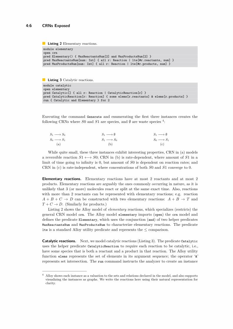
4:6 CRNs Exposed
Listing 2 Elementary reactions.module elementaryopen crnpred Elementary() MaxReactantsNum[2] and MaxProductsNum[2] pred MaxReactantsNum[num: Int] all r: Reaction | lte[#r.reactants, num] pred MaxProductsNum[num: Int] all r: Reaction | lte[#r.products, num]
Listing 3 Catalytic reactions.module catalyticopen elementarypred Catalytic[] all r: Reaction | CatalyticReaction[r] pred CatalyticReaction[r: Reaction] some elems[r.reactants] & elems[r.products] run Catalytic and Elementary for 2
Executing the command Generate and enumerating the first three instances creates thefollowing CRNs where S0 and S1 are species, and ∅ are waste species 4:
S1 −−→ S0
S0 −−→ S1
S1 −−→ ∅S1 −−→ S0
S1 −−→ ∅S0 −−→ S1
(a) (b) (c)
While quite small, these three instances exhibit interesting properties, CRN in (a) modelsa reversible reaction S1 ←→ S0; CRN in (b) is rate-dependent, where amount of S1 in alimit of time going to infinity is 0, but amount of S0 is dependent on reaction rates; andCRN in (c) is rate-independent, where concentrations of both S0 and S1 converge to 0.
Elementary reactions. Elementary reactions have at most 2 reactants and at most 2products. Elementary reactions are arguably the ones commonly occurring in nature, as it isunlikely that 3 (or more) molecules react or split at the same exact time. Also, reactionswith more than 2 reactants can be represented with elementary reactions; e.g. reactionA + B + C → D can be constructed with two elementary reactions: A + B → T andT + C → D. (Similarly for products.)
Listing 2 shows the Alloy model of elementary reactions, which specializes (restricts) thegeneral CRN model crn. The Alloy model elementary imports (open) the crn model anddefines the predicate Elementary, which uses the conjunction (and) of two helper predicatesMaxReactantsNum and MaxProductsNum to characterize elementary reactions. The predicatelte is a standard Alloy utility predicate and represents the ≤ comparison.
Catalytic reactions. Next, we model catalytic reactions (Listing 3). The predicate Catalyticuses the helper predicate CatalyticReaction to require each reaction to be catalytic, i.e.,have some species that is both a reactant and a product in that reaction. The Alloy utilityfunction elems represents the set of elements in its argument sequence; the operator ‘&’represents set intersection. The run command instructs the analyzer to create an instance
4 Alloy shows each instance as a valuation to the sets and relations declared in the model, and also supportsvisualizing the instances as graphs. We write the reactions here using their natural representation forclarity.
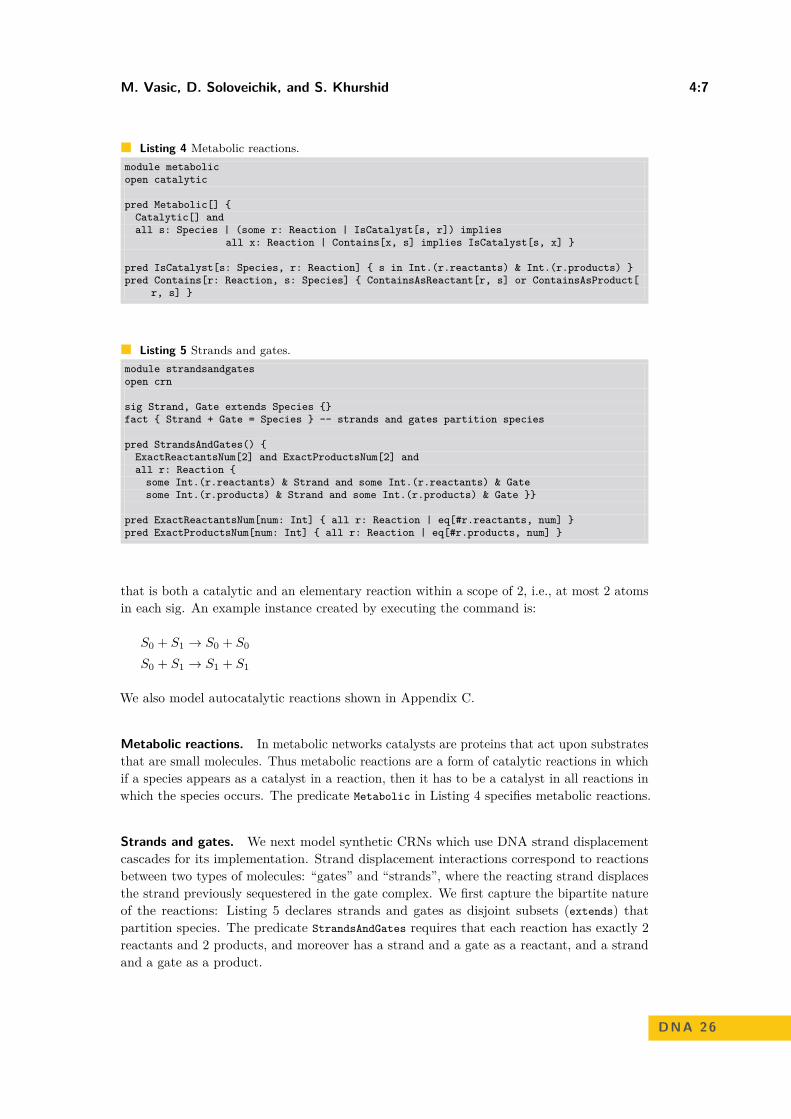
M. Vasic, D. Soloveichik, and S. Khurshid 4:7
Listing 4 Metabolic reactions.module metabolicopen catalytic
pred Metabolic[] Catalytic[] andall s: Species | (some r: Reaction | IsCatalyst[s, r]) implies
all x: Reaction | Contains[x, s] implies IsCatalyst[s, x]
pred IsCatalyst[s: Species, r: Reaction] s in Int.(r.reactants) & Int.(r.products) pred Contains[r: Reaction, s: Species] ContainsAsReactant[r, s] or ContainsAsProduct[
r, s]
Listing 5 Strands and gates.module strandsandgatesopen crn
sig Strand, Gate extends Species fact Strand + Gate = Species -- strands and gates partition species
pred StrandsAndGates() ExactReactantsNum[2] and ExactProductsNum[2] andall r: Reaction some Int.(r.reactants) & Strand and some Int.(r.reactants) & Gatesome Int.(r.products) & Strand and some Int.(r.products) & Gate
pred ExactReactantsNum[num: Int] all r: Reaction | eq[#r.reactants, num] pred ExactProductsNum[num: Int] all r: Reaction | eq[#r.products, num]
that is both a catalytic and an elementary reaction within a scope of 2, i.e., at most 2 atomsin each sig. An example instance created by executing the command is:
S0 + S1 → S0 + S0
S0 + S1 → S1 + S1
We also model autocatalytic reactions shown in Appendix C.
Metabolic reactions. In metabolic networks catalysts are proteins that act upon substratesthat are small molecules. Thus metabolic reactions are a form of catalytic reactions in whichif a species appears as a catalyst in a reaction, then it has to be a catalyst in all reactions inwhich the species occurs. The predicate Metabolic in Listing 4 specifies metabolic reactions.
Strands and gates. We next model synthetic CRNs which use DNA strand displacementcascades for its implementation. Strand displacement interactions correspond to reactionsbetween two types of molecules: “gates” and “strands”, where the reacting strand displacesthe strand previously sequestered in the gate complex. We first capture the bipartite natureof the reactions: Listing 5 declares strands and gates as disjoint subsets (extends) thatpartition species. The predicate StrandsAndGates requires that each reaction has exactly 2reactants and 2 products, and moreover has a strand and a gate as a reactant, and a strandand a gate as a product.
DNA 26

4:8 CRNs Exposed
t* t*
t
t
b*
b
b
a
c+
t* t*
t
t
b*
b
b
a
c
+
(strand)
(left gate)
(strand)
(right gate)
Figure 2 DNA strand displacement reaction with the seesaw gate motif. There are two reactants(a strand and a gate) and two products (a strand and a gate). A gate consists of two strands boundtogether. (For simplicity the usual helical structure of DNA is not shown.) Labels show bindingsites (domains); a star indicates Watson-Crick complement such that domain x binds x∗. In orderfor the reaction to happen, the complementary domains must match as shown. Such reactions canbe cascaded since the strands < a, t, b > and < b, t, c > can react with other seesaw gates.
Seesaw networks. A simple yet powerful subclass of DNA strand displacement reactions isthe “seesaw” model. Seesaw reactions have been used to create some of the largest syntheticbiochemical reaction networks, including logic circuits and neural networks [13, 49]. Themolecular structure schematic for a seesaw reaction is shown in Figure 2. Listing 6 modelsseesaw reactions by specializing the model of strands and gates (Listing 5), capturing theabstract molecular structure in an Alloy model. The signature Domain models the bindingdomains. The signature DNASpecies is a subset (in) of species, and left and right arebinary relations that map DNASpecies to their left and right domains respectively. Thekeyword lone constraints the relations to be partial functions. The signatures RightGateand LeftGate partition gates. The fact UseAll requires all species to be DNA species, andrequires all domains to be a part of some species . The fact UniqueSpecies enforces thatstrands and gates are unique, i.e., there cannot be two or more strands (or left/right gates)with matching left and right domains. The fact OneDomain requires strands and gates to haveexactly one left and exactly one right domain. The predicate CanReactStrandAndLeftGateis true if inputs (reactants) conform to the interaction rules of a strand and a left gate,similar holds for the predicate CanReactStrandAndRightGate on strands and right gates. Thepredicate CanReact is true if inputs (reactants) satisfy either CanReactStrandAndLeftGateor CanReactStrandAndRightGate. The predicate ReactStrandAndLeftGate is true if inputs(reactants and products) conform to the interaction rules of a strand and a left gate,specifically s and lg interact, i.e., the right domain of s matches the left domain of lg,and produce s’ and rg’ where the left and right domains of s’ match those of lg, andleft and right domains of rg’ match those of s; likewise, ReactStrandAndRightGate specifiesthe interaction of a strand and a right gate. The functions ReactantsSet and ProductsSetreturns a set of reactants (products) in a reaction. The predicate Seesaw specifies: (a) eachreaction to be a seesaw reaction by enforcing the predicate React on every reaction; (b) thatall possible reactions exist, i.e., if two species can interact based on seesaw interaction rules(predicate CanReact) than a reaction containing those species as reactants (or products) mustexist; (c) that reactions only in one direction exist (to reduce number of solutions we enforcethat only one direction of reaction exist in enumerated CRNs knowing that seesaw reactionsare always reversible); (d) that reactions have a left gate as a reactant (this is to preventmultiple redundant solutions, since all reactions are reversible we can enforce that left gateis always on the left hand side).
An instance generated by Alloy running the predicate with command GenSeesaw isSab + LGbc → Sbc + RGab, where Sab and Sbc are strands, LGbc left gate, RGab right gate,while left and right domains a, b, c are denoted in subscript. Note that this reaction isequivalent to the one shown in Figure 2.
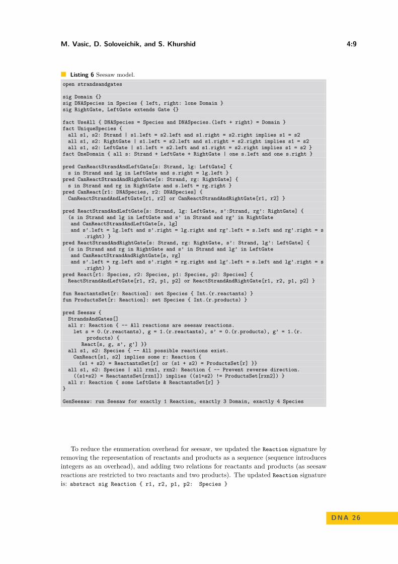
M. Vasic, D. Soloveichik, and S. Khurshid 4:9
Listing 6 Seesaw model.open strandsandgates
sig Domain sig DNASpecies in Species left, right: lone Domain sig RightGate, LeftGate extends Gate
fact UseAll DNASpecies = Species and DNASpecies.(left + right) = Domain fact UniqueSpecies all s1, s2: Strand | s1.left = s2.left and s1.right = s2.right implies s1 = s2all s1, s2: RightGate | s1.left = s2.left and s1.right = s2.right implies s1 = s2all s1, s2: LeftGate | s1.left = s2.left and s1.right = s2.right implies s1 = s2
fact OneDomain all s: Strand + LeftGate + RightGate | one s.left and one s.right
pred CanReactStrandAndLeftGate[s: Strand, lg: LeftGate] s in Strand and lg in LeftGate and s.right = lg.left
pred CanReactStrandAndRightGate[s: Strand, rg: RightGate] s in Strand and rg in RightGate and s.left = rg.right
pred CanReact[r1: DNASpecies, r2: DNASpecies] CanReactStrandAndLeftGate[r1, r2] or CanReactStrandAndRightGate[r1, r2]
pred ReactStrandAndLeftGate[s: Strand, lg: LeftGate, s’:Strand, rg’: RightGate] (s in Strand and lg in LeftGate and s’ in Strand and rg’ in RightGateand CanReactStrandAndLeftGate[s, lg]and s’.left = lg.left and s’.right = lg.right and rg’.left = s.left and rg’.right = s
.right) pred ReactStrandAndRightGate[s: Strand, rg: RightGate, s’: Strand, lg’: LeftGate] (s in Strand and rg in RightGate and s’ in Strand and lg’ in LeftGateand CanReactStrandAndRightGate[s, rg]and s’.left = rg.left and s’.right = rg.right and lg’.left = s.left and lg’.right = s
.right) pred React[r1: Species, r2: Species, p1: Species, p2: Species] ReactStrandAndLeftGate[r1, r2, p1, p2] or ReactStrandAndRightGate[r1, r2, p1, p2]
fun ReactantsSet[r: Reaction]: set Species Int.(r.reactants) fun ProductsSet[r: Reaction]: set Species Int.(r.products)
pred Seesaw StrandsAndGates[]all r: Reaction -- All reactions are seesaw reactions.let s = 0.(r.reactants), g = 1.(r.reactants), s’ = 0.(r.products), g’ = 1.(r.
products) React[s, g, s’, g’]
all s1, s2: Species -- All possible reactions exist.CanReact[s1, s2] implies some r: Reaction (s1 + s2) = ReactantsSet[r] or (s1 + s2) = ProductsSet[r]
all s1, s2: Species | all rxn1, rxn2: Reaction -- Prevent reverse direction.((s1+s2) = ReactantsSet[rxn1]) implies ((s1+s2) != ProductsSet[rxn2])
all r: Reaction some LeftGate & ReactantsSet[r]
GenSeesaw: run Seesaw for exactly 1 Reaction, exactly 3 Domain, exactly 4 Species
To reduce the enumeration overhead for seesaw, we updated the Reaction signature byremoving the representation of reactants and products as a sequence (sequence introducesintegers as an overhead), and adding two relations for reactants and products (as seesawreactions are restricted to two reactants and two products). The updated Reaction signatureis: abstract sig Reaction r1, r2, p1, p2: Species
DNA 26
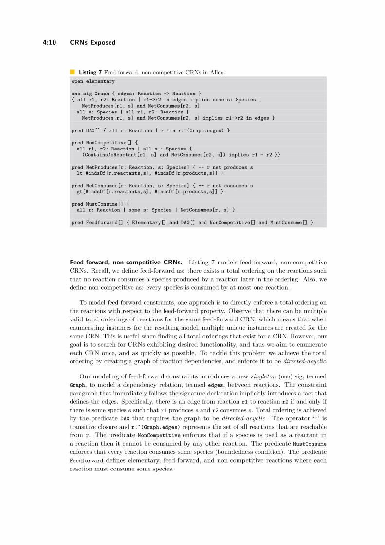
4:10 CRNs Exposed
Listing 7 Feed-forward, non-competitive CRNs in Alloy.open elementary
one sig Graph edges: Reaction -> Reaction all r1, r2: Reaction | r1->r2 in edges implies some s: Species |
NetProduces[r1, s] and NetConsumes[r2, s]all s: Species | all r1, r2: Reaction |NetProduces[r1, s] and NetConsumes[r2, s] implies r1->r2 in edges
pred DAG[] all r: Reaction | r !in r.^(Graph.edges)
pred NonCompetitive[] all r1, r2: Reaction | all s : Species (ContainsAsReactant[r1, s] and NetConsumes[r2, s]) implies r1 = r2
pred NetProduces[r: Reaction, s: Species] -- r net produces slt[#indsOf[r.reactants,s], #indsOf[r.products,s]]
pred NetConsumes[r: Reaction, s: Species] -- r net consumes sgt[#indsOf[r.reactants,s], #indsOf[r.products,s]]
pred MustConsume[] all r: Reaction | some s: Species | NetConsumes[r, s]
pred Feedforward[] Elementary[] and DAG[] and NonCompetitive[] and MustConsume[]
Feed-forward, non-competitive CRNs. Listing 7 models feed-forward, non-competitiveCRNs. Recall, we define feed-forward as: there exists a total ordering on the reactions suchthat no reaction consumes a species produced by a reaction later in the ordering. Also, wedefine non-competitive as: every species is consumed by at most one reaction.
To model feed-forward constraints, one approach is to directly enforce a total ordering onthe reactions with respect to the feed-forward property. Observe that there can be multiplevalid total orderings of reactions for the same feed-forward CRN, which means that whenenumerating instances for the resulting model, multiple unique instances are created for thesame CRN. This is useful when finding all total orderings that exist for a CRN. However, ourgoal is to search for CRNs exhibiting desired functionality, and thus we aim to enumerateeach CRN once, and as quickly as possible. To tackle this problem we achieve the totalordering by creating a graph of reaction dependencies, and enforce it to be directed-acyclic.
Our modeling of feed-forward constraints introduces a new singleton (one) sig, termedGraph, to model a dependency relation, termed edges, between reactions. The constraintparagraph that immediately follows the signature declaration implicitly introduces a fact thatdefines the edges. Specifically, there is an edge from reaction r1 to reaction r2 if and only ifthere is some species s such that r1 produces s and r2 consumes s. Total ordering is achievedby the predicate DAG that requires the graph to be directed-acyclic. The operator ‘ˆ’ istransitive closure and r.ˆ(Graph.edges) represents the set of all reactions that are reachablefrom r. The predicate NonCompetitive enforces that if a species is used as a reactant ina reaction then it cannot be consumed by any other reaction. The predicate MustConsumeenforces that every reaction consumes some species (boundedness condition). The predicateFeedforward defines elementary, feed-forward, and non-competitive reactions where eachreaction must consume some species.

M. Vasic, D. Soloveichik, and S. Khurshid 4:11
Algorithm 1 Search Algorithm.Input: Model (model), Generation bounds (scope), Function (f), Inputs (N).Output: CRN that computes f if found; otherwise, null.
1: procedure ExhaustiveSearch2: for each instance ∈ Alloy.findAllInstances(model, scope) do3: crn← translate(instance)4: if ComputesF (crn, f, N) then return crn5: end for6: return null7: end procedure
3 CRN Enumeration and Search
In this section we describe our algorithm (shown in Algorithm 1) that performs a boundedexhaustive search enumerating all CRNs in a given class and within a given bounds respectingproperties defined by an Alloy model, to find the CRN implementing desired function.
Inputs to the algorithm are the Alloy model, the size of CRNs (e.g., number of reactionsand species) defined by the scope, desired target function f , and the number of inputs to thefunction N . Function findAllInstances accepts the Alloy model definition and scope, andenumerates all possible instances that satisfy the Alloy model. Each Alloy instance istranslated to CRN (step 3). Then, in step 4 we invoke the Algorithm 2 (Section 4) to checkif CRN computes f . If CRN implementing given function is found then it is returned (step4). If after checking all instances no satisfying CRN is found then the procedure returns null.
Bounded exhaustive search . To find the smallest CRN computing f we conduct a boundedexhaustive search. Our goal is to find a smallest (in terms of numbers of species and reactions)feed-forward, non-competitive CRN that computes f . We use iterative deepening [26, 28,30]where we start from a small scope and iteratively increase it to a larger scope until a desiredCRN is found, where for each scope we invoke Algorithm 1.
4 CRN Analysis
In this section we describe our algorithm for checking if a CRN computes a function ofinterest (f).
Conservation Equations. We first construct a set of conservation equations for the CRNwhich describe concentrations of species in terms of their initial concentrations and reactionfluxes. A reaction flux is equal to the total “flow of material” through the reaction. Weassociate a flux variable to the each reaction, where fluxi represents the flux of the reactioni. Then the concentration of a species S can be expressed in terms of its initial concentrationS0 and reaction fluxes:
s = s0 +N∑
i=1
netGain(rxni, S) · fluxi (1)
where netGain(rxni, S) is the net stoichiometric gain of species S in the reaction i (negativein the case of loss), and N is the number of reactions in the CRN. For example, the CRNfrom Figure 1 generates the equations shown in 2. The variables on the left side of equationsrepresent concentrations of species, variables with suffixes 0 represent initial concentrations of
DNA 26

4:12 CRNs Exposed
species (e.g., z10 is initial concentration of species Z1), and finally fluxi variables representfluxes of reactions.
a = a0 − flux1 b = b0 − flux2
z1 = z10 + flux1 − flux3 z2 = z20 + flux2 − flux3
k = k0 + flux3 − flux4 y = y0 + flux1 + flux2 − flux4
(2)
Equilibrium Condition. We next use the above conservation equations to find equilibria.Since we focus on rate-independent computation, we search for static equilibria only (noneof the reactions is occurring).5 A static equilibrium corresponds to every reaction having atleast one reactant in zero concentration. Thus, we create multiple systems of equations fromthe conservation equations, where each system corresponds to setting concentrations of a setof species to zero, where the set contains a reactant from each reaction. The solution of eachsuch constructed system of equations represents concentrations of species at an equilibrium.Different equilibria will be reached from different initial conditions.
As an example, consider again the CRN shown in Figure 1. All combinations of speciescontaining a reactant from each reaction are: (A, B, Z1, Y ), (A, B, Z2, Y ), (A, B, Z1, K),(A, B, Z2, K). For each combination we set its species concentrations to zero and solve thesystem 2. This results in 4 solutions shown in 3 (we do not show solutions for flux variablesdue to the space limits).
a b k y z1 z2
0 0 −b0 + k0 − y0 + z10 0 0 −a0 + b0 − z10 + z20
0 0 −a0 + k0 − y0 + z20 0 a0 − b0 + z10 − z20 00 0 0 b0 − k0 + y0 − z10 0 −a0 + b0 − z10 + z20
0 0 0 a0 − k0 + y0 − z20 a0 − b0 + z10 − z20 0(3)
Although there are 4 solutions, for any particular initial concentrations of the species onlyone of the solutions is non-negative (concentrations of species must be non-negative), andthus feasible.
Check whether CRN computes f . We then check if the equilibrium solutions are equivalentto f . In general, we do not know which species correspond to the input and which to theoutput, and thus we need to check for all possible combinations of the input and the outputspecies. First, we construct all input n-tuples without repeating elements from a set ofspecies (where n is the number of the inputs to f)6. Second, for all species that are notin the input tuple we set initial concentrations to zero. Third, for the output species wetry any of the remaining species. Fourth, for a given set of input and output species, weconstruct a piecewise function, where each solution is valid if concentrations of species arenon-negative. Finally, we use Mathematica’s constraint solving procedure FindInstance tocheck if the constructed piecewise function differs from function f .
5 In chemical kinetics, static equilibrium refers to an equilibrium where none of the reactions occur. Incontrast, in dynamic equilibria, concentrations don’t change over time because the effects of the differentreactions cancel out. Note that dynamic equilibria are not rate-independent since changing a reactionrate affects the equilibrium concentrations of the species involved in that reaction.
6 An input tuple (a,b) will be separately considered from (b,a). However, if the sought function is knownto be commutative than the order of species can be ignored.

M. Vasic, D. Soloveichik, and S. Khurshid 4:13
Algorithm 2 ComputesF.Input: CRN crn, Function f , Number of inputs N .Output: True if crn computes f ; false otherwise.
1: procedure ComputesF2: conservationEquations← constructConservationEquations(crn)3: equilibriumSolutions← ∅4: for each speciesSet ∈ getAllReactantCombinations(crn) do5: equilibriumEquations← setConcT oZero(conservationEquations, speciesSet)6: solution← solve(equilibriumEquations)7: equilibriumSolutions.add(solution)8: end for9: for each x1, x2, ..., xN , y ∈ getInputOutputSpecies(crn, N) do10: nonInputSpecies← getOtherSpecies(crn, x1, x2, ..., xn)11: newSols← setInitialConcT oZero(equilibriumSolutions, nonInputSpecies)12: pwF ← constructP iecewise(newSols, y)13: counterExample← F indInstance(pwF 6= f(x1, x2, ..., xN ))14: if counterExample = null then return true15: end for16: return false17: end procedure
To illustrate on our example, consider setting input species to A and B, and output to Y .The system of equations 3 reduces to the system 4.
a b k y z1 z2
0 0 −b0 0 0 −a0 + b0
0 0 −a0 0 a0 − b0 00 0 0 b0 0 −a0 + b0
0 0 0 a0 a0 − b0 0
(4)
The first two solutions are infeasible since they result in species k having negative con-centration, −b0 and −a0. More precisely they are feasible only in the trivial case wherea0 = 0 ∧ b0 = 0. The third solution is feasible when b0 ≥ a0, in which case y = b0; whilefourth solution is feasible when a0 ≥ b0, in which case y = a0. Thus, we can construct thepiecewise function unifying multiple equilibrium solutions into a single function:
y =
b0 b0 ≥ a0
a0 a0 ≥ b0
Next, once we constructed the equilibrium piecewise function (y(a0, b0)) we invoke theMathematica’s constraint solving procedure FindInstance to find an assignment of inputs(a0, b0) for which y differs from f , with additional condition that initial concentrations arenon-negative (a0 ≥ 0 ∧ b0 ≥ 0). If no counterexample is found, then the CRN computes f
and we have finished our search. On the other hand, if a counterexample is found, thenwe repeat the procedure for the next combination of input and output species. When thelist of input and output combinations is exhausted we can conclude that the CRN does notcompute f .
Algorithm. We implement this functionality in Mathematica by defining ComputesF func-tion described in Algorithm 2. In step 2, conservation equations are constructed, while instep 3 we initialize a set of equilibrium solutions equilibriumSolutions to an empty set. Insteps 4–8, we iterate over all existing sets of species containing at least one reactant from eachreaction. Specifically, function getAllReactantCombinations computes Cartesian product oversets of reactants from different reactions; and removes elements with the same sets of species.In step 5 we update the conservation equations by setting speciesSet concentrations to zero,
DNA 26

4:14 CRNs Exposed
Table 1 Number of enumerated feed-forward, non-competitive CRNs and wall-clock times(hh:mm:ss) for the enumeration procedure.
1 Reaction 2 Reactions 3 Reactions 4 Reactions
1 Species 3 00:00:00 0 00:00:00 0 00:00:00 0 00:00:002 Species 10 00:00:00 22 00:00:00 0 00:00:00 0 00:00:003 Species 6 00:00:00 199 00:00:00 287 00:00:00 0 00:00:004 Species 1 00:00:00 391 00:00:00 4,666 00:00:05 5,643 00:00:075 Species 0 00:00:00 291 00:00:00 17,509 00:00:19 140,064 00:03:576 Species 0 00:00:00 100 00:00:00 27,257 00:00:32 817,742 00:30:35
and save the linear system in equilibriumEquations. In steps 6–7 we solve the system oflinear equations and add it to the list of equilibrium solutions (note that since we are focusedon feed-forward non-competitive reactions, a unique solution will always exist). Next, weiterate over all combinations of input and output species x1, x2, ..., xN , y, where x1, x2,..., xN represent input species, and y output species. In step 10 we get all the species thatare not in the input species set. In step 11 we modify the equilibrium solutions by settinginitial concentrations of nonInputSpecies to zero, and we save the result in newSols. Instep 12 we construct a piecewise function pwF out of newSols. Finally, in step 13 we invokethe FindInstance method to find input values for which pwF is different then f . If suchsolution is not found then counterExample is null, and constructed pwF is implementingf ; in which case procedure returns true. If counterexample is found then the same stepsare repeated for different set of input and output species. Finally, if all combinations areexhausted procedure returns false.
5 New Results
In this section we present new discoveries made using the proposed techniques. We focus onthe class of feed-forward, non-competitive CRNs since they are always rate-independent.
Smallest max CRN. We perform bounded exhaustive search for 1 to 4 reactions, and 1–6species, starting with smaller number of species and reactions, and iteratively increasing thescope until the max is found. Table 1 shows the number of enumerated CRNs and Alloyenumeration time for different scope sizes. We perform (not perfect) isomorphic breakingin Alloy by requiring lexicographic ordering on reactions among other things (details ofsymmetry breaking are shown in Appendix F). Note that while we perform some isomorphicbreaking7, not all isomorphic cases are pruned, and thus number of non-isomorphic instancesmay be less then numbers reported in Table 1. In spite of this, our approach is still exhaustive,meaning that all possible CRNs will be enumerated, but some may be enumerated multipletimes. The first occurrence of max is found in the scope of 4 reactions and 6 species, andit was the 124, 118th instance Alloy enumerated in that scope. The CRN discovered isequivalent to the one shown in Figure 1, modulo reaction and species ordering.
7 Alloy can generate isomorphic instances, i.e., two instances that are distinct but there exists a permutationon atoms, which maps one instance to the other

M. Vasic, D. Soloveichik, and S. Khurshid 4:15
X+ −−→M + Y +
M + X− −−→ Y −
X+ −−→ Y + + C
X− −−→ Y + + E
C + E −−→ 2 Y −
X+1 −−→M1 + Y +
max
X−1 −−→M2 + Y −
min
X+2 −−→M2 + Y +
max
X−2 −−→M1 + Y −
min
M1 + M2 −−→ Y −max + Y +
min
Figure 3 Minimal ReLU (left), abs (middle) and minmax (right) CRNs. (left) The ReLUCRN produces x+(0) amount of M and Y + by the first reaction. The second reaction producesmin(x+(0), x−(0)) amount of Y −. Thus, the amount of output produced is: y = y+ − y− =x+(0)−min(x+(0), x−(0)) which can be shown to be equal to ReLU(x+(0)− x+(0)) = ReLU(x).(middle) The abs CRN produces x+(0) amount of C and E by the first and second reactions,respectively, x+(0) + x−(0) amount of Y +, and 2min(x+(0), x−(0)) amount of Y −. Thus, y =x+(0) + x−(0)− 2min(x+(0), x−(0)) = abs(x+(0), x−(0)) = abs(x).
Dual-rail convention. Concentrations of species are always non-negative, making it im-possible to represent negative values directly. However, there is a natural way to extendcomputation semantics to negative values. Instead of using a single species to represent avalue, in dual-rail convention a value is represented by a difference between a two species(e.g., the output value is equal to the concentration of species Y + minus that of Y −).
An additional requirement for CRN modules is to be composable, in the sense that theoutput of one can be input to another. Note, for example, that the max system (Figure 1) isnot composable because the downstream module might consume some amount of Y before itis consumed in its interaction with K (last reaction). Composability can be ensured if theoutput species are never consumed [9,14,52]. Note that consuming Y + is logically equivalentto producing Y − (and vise versa for Y −), and thus we restrict dual-rail computation in thisway without losing expressibility.
Smallest ReLU CRN. Using the above described procedure we run experiments for findingthe smallest CRN computing ReLU (rectified linear unit) function. We confirm that theCRN introduced in [58], which is shown in Figure 3, is indeed the smallest. Note that CRNswere already enumerated when searching for max, and that was no need to re-enumeratethem as they were saved on disk.
Our analysis shows that the ReLU CRN is the smallest in the sense that there is no otherCRN computing this function with fewer than 2 reactions or 5 species. In Appendix D weargue that our enumeration in Table 1 is sufficient to ensure that 5 species are necessary nomatter how many reactions are allowed.
Smallest abs CRN. We conducted a similar experiment for finding the smallest CRNcomputing the absolute value function, finding CRN shown in Figure 3.
Smallest minmax CRN. Minmax CRN accepts two inputs and has two outputs, where oneoutput computes max, and other output computes min of the inputs. Since species are indual-rail form, there is 4 input and 4 output species. Thus, for minmax search we enumeratedCRNs that have at least 8 species, where at least 4 species only appear as products (outputspecies candidates), and at least 4 species which do not appear only as products (inputspecies candidates). We have further restricted the CRNs to have a total of at most 16reactants and products over all reactions. Enumeration results with those constraints areshown in Table 2 (isomorphic breaking is imperfect in this case as well). We discovered the
DNA 26

4:16 CRNs Exposed
Table 2 Number of enumerated feed-forward, non-competitive CRNs with at least two dual-railinputs (4 actual species) and two outputs (4 actual species). Star (∗) denotes that the scope hasbeen partially enumerated.
2 Reactions 3 Reactions 4 Reactions 5 Reactions
8 Species 1 00:00:00 1,176 00:00:03 67,323 00:03:09 0 00:00:009 Species 0 00:00:00 1,073 00:00:03 223,775 00:12:48 2,439,310 13:31:1910 Species 0 00:00:00 385 00:00:02 328,397 00:19:30 4,669,000∗ 47:39:39
Table 3 Number of enumerated seesaw reactions with different number of domains and reactions,and up to 20 distinct species.
1 Reaction 2 Reactions 3 Reactions 4 Reactions 5 Reactions
1 Domain 1 00:00:00 0 00:00:00 0 00:00:00 0 00:00:00 0 00:00:002 Domains 1 00:00:00 4 00:00:00 0 00:00:00 2 00:00:01 1 00:00:033 Domains 1 00:00:00 5 00:00:00 15 00:00:01 13 00:00:05 14 00:00:174 Domains 0 00:00:00 9 00:00:01 33 00:00:02 92 00:00:18 121 00:01:585 Domains 0 00:00:00 4 00:00:00 55 00:00:04 243 00:00:48 705 00:10:166 Domains 0 00:00:00 1 00:00:00 43 00:00:10 436 00:06:40 2027 03:01:06
minimal minmax CRN, which is shown in Figure 3. We performed several optimizations tospeed up the analysis phase which are described in Appendix E.
Seesaw enumeration. We enumerated all nonisomorphic seesaw CRNs up to specifiedbounds on the number of domains and reactions. Table 3 shows the number of enumeratedCRNs restricted to 1-5 reactions, 1-6 domains, and up to 20 species. Since 5 seesaw reactionscan have at most 20 distinct species this includes all possible seesaw CRNs in the scope of 1-5reactions. For seesaw networks, we define isomorphic CRNs as those that can be obtainedby: (a) swapping domain names, (b) changing order of reactants or products, (c) changingorder of reactions, (d) swapping reactants with products (follows from the reversibility ofseesaw reactions).
In order to check for isomorphisms while enumerating seesaw CRNs, we maintain a setof previously enumerated CRNs and all their isomorphisms. If a newly enumerated CRNis not found in the current set, we create the isomorphic class of the CRN by making allpermutations of the CRN, and adding them to the set. Permutations are done only withrespect to domains. Permuting the order of reactants and products, as well as swappingreactants and products, is not needed as we follow the convention of enumerating CRNsin a form S?? + LG?? ↔ S?? + RG??. Permuting the order of reactions is not needed, asthe set of CRNs is preserved as a hash table where a custom-made hash function is usedfor CRNs (a same hash value is returned for a CRN irrespective of the order of reactions).The isomorphic breaking is implemented as a post-processing step in Java. The run-timesreported in Table 3 include both generation and isomorphic breaking times.
Note that we require that the CRN corresponding to a seesaw system contain all reactionsthat can occur. For illustration, we analyze seesaw CRNs with 2 domains and 1 reaction.Due to the reversibility of seesaw reactions we can limit our analysis to CRNs that have aleft gate on the left hand side; thus our CRN will be of the form S?? + LG?? ↔ S?? + RG??,where ? represent domains to be filled in. We denote two available domains with a and b,
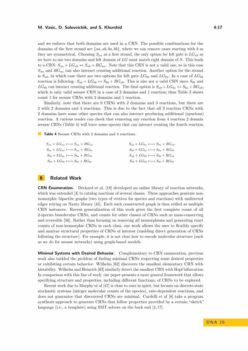
M. Vasic, D. Soloveichik, and S. Khurshid 4:17
and we enforce that both domains are used in a CRN. The possible combinations for thedomains of the first strand are aa, ab, ba, bb, where we can remove cases starting with b asthey are symmetrical. Choosing Saa as a first strand, the only option for left gate is LGab aswe have to use two domains and left domain of LG must match right domain of S. This leadsto a CRN: Saa + LGab ↔ Sab + RGaa. Note that this CRN is not a valid one, as in this caseSaa and RGaa can also interact creating additional reaction. Another option for the strandis Sab, in which case there are two options for left gate LGbb and LGba. In a case of LGbb
reaction is following: Sab + LGbb ↔ Sbb + RGab. This is also not a valid CRN since Sbb andLGbb can interact creating additional reaction. The final option is Sab + LGba ↔ Sba + RGab,which is only valid seesaw CRN in a case of 2 domains and 1 reaction; thus Table 3 showscount 1 for seesaw CRNs with 2 domains and 1 reaction.
Similarly, note that there are 0 CRNs with 2 domains and 3 reactions, but there are2 with 2 domains and 4 reactions. This is due to the fact that all 3 reaction CRNs with2 domains have some other species that can also interact producing additional (spurious)reaction. A curious reader can check that removing any reaction from 4 reaction 2 domainseesaw CRNs (Table 4) will leave some species that can interact creating the fourth reaction.
Table 4 Seesaw CRNs with 2 domains and 4 reactions.
Saa + LGaa ←−→ Saa + RGaa
Sba + LGaa ←−→ Saa + RGba
Sbb + LGba ←−→ Sba + RGbb
Sbb + LGbb ←−→ Sbb + RGbb
Sab + LGba ←−→ Sba + RGab
Sbb + LGba ←−→ Sba + RGbb
Sab + LGbb ←−→ Sbb + RGab
Sbb + LGbb ←−→ Sbb + RGbb
6 Related Work
CRN Enumeration. Deckard et al. [18] developed an online library of reaction networks,which was extended [3] to catalog reactions of several classes. These approaches generate non-isomorphic bipartite graphs (two types of vertices for species and reactions) with undirectededges relying on Nauty library [45]. Each such constructed graph is then reified as multipleCRN instances. Recent generalization of this work gives the first complete count of all2-species bimolecular CRNs, and counts for other classes of CRNs such as mass-conservingand reversible [56]. Rather than focusing on removing all isomorphisms and generating exactcounts of non-isomorphic CRNs in each class, our work allows the user to flexibly specifyand analyze structural properties of CRNs of interest (enabling direct generation of CRNsfollowing the structure). For example, it is not clear how to encode molecular structure (suchas we do for seesaw networks) using graph-based models.
Minimal Systems with Desired Behavior. Complementary to CRN enumeration, previouswork also tackled the problem of finding minimal CRNs respecting some desired propertiesor exhibiting certain behavior. Wilhelm [62] discovers the smallest elementary CRN withbistability. Wilhelm and Heinrich [63] similarly detect the smallest CRN with Hopf bifurcation.In comparison with this line of work, our paper presents a more general framework that allowsspecifying structure and properties, including different functions, of CRNs to be explored.
Recent work due to Murphy et al [47] is close to ours in spirit, but focuses on discrete-statestochastic systems (integer molecular counts of the species), rate-dependent reactions, anddoes not guarantee that discovered CRNs are minimal. Cardelli et al [8] take a programsynthesis approach to generate CRNs that follow properties provided by a certain “sketch”language (i.e., a template) using SMT solvers on the back end [4, 17].
DNA 26
4:18 CRNs Exposed
Computational power of CRNs. Much ongoing work has explored computational power ofCRNs [31,43,51,59]. It is shown how to map complex computation to CRNs, such as mappingpolynomials to chemical reactions, mapping discrete algorithms, and even defining a high-levelimperative languages that map to CRNs. We believe that by exploring CRNs bottom up, wemay found answers of what the appropriate (more efficient) high-level primitives are to beused for implementing such high-level functionality.
7 Conclusion
We introduced the use of Alloy, a framework for modeling and analyzing structural constraintsand behavior in software systems, to enumerate CRNs with declaratively specified properties.We showed how this framework can enumerate CRNs with a variety of structural constraintsincluding biologically motivated catalytic networks and metabolic networks, and seesawnetworks motivated by DNA nanotechnology. We also used the framework to explore analogfunction computation in rate-independent CRNs. We applied our approach in a case-studyto find the smallest CRNs computing the max, minmax, abs and ReLU functions in a naturalsubclass of rate-independent CRNs where rate-independence follows from structural networkproperties.
There remain a number of open questions that motivate future research directions. Animportant area of optimization is improving the run-time of the Alloy enumeration. Canwe optimize the isomorphic breaking process to eliminate all isomorphisms? For improvedefficiency and ease of use, do we need to rely on a separate tool like Mathematica to determinewhether a given CRN computes the desired function, or can the necessary functionality beperformed in Alloy alone? Finally, it remains to be seen how easily the techniques developedin this paper could be applied to rate-dependent computation.
References1 Dana Angluin, James Aspnes, and David Eisenstat. A simple population protocol for fast
robust approximate majority. Distributed Computing, 21(2):87–102, 2008.2 Dana Angluin, James Aspnes, David Eisenstat, and Eric Ruppert. The computational power
of population protocols. Distributed Computing, 20(4):279–304, 2007.3 Murad Banaji. Counting chemical reaction networks with NAUTY. arXiv preprint
arXiv:1705.10820, 2017.4 Clark Barrett, Christopher L. Conway, Morgan Deters, Liana Hadarean, Dejan Jovanović,
Tim King, Andrew Reynolds, and Cesare Tinelli. CVC4. In CAV, 2011.5 Gilles Bernot, Jean-Paul Comet, Adrien Richard, and Janine Guespin. Application of formal
methods to biological regulatory networks: extending thomas’ asynchronous logical approachwith temporal logic. Journal of theoretical biology, 2004.
6 Luca Cardelli. Strand algebras for DNA computing. Natural Computing, 10(1):407–428, 2011.7 Luca Cardelli. Morphisms of reaction networks that couple structure to function. BMC
systems biology, 8(1):84, 2014.8 Luca Cardelli, Milan Češka, Martin Fränzle, Marta Kwiatkowska, Luca Laurenti, Nicola
Paoletti, and Max Whitby. Syntax-guided optimal synthesis for chemical reaction networks.In CAV, 2017.
9 Cameron Chalk, Niels Kornerup, Wyatt Reeves, and David Soloveichik. Composable rate-independent computation in continuous chemical reaction networks. In CMSB, pages 256–273.Springer, 2018.
10 Ho-Lin Chen, David Doty, and David Soloveichik. Deterministic function computation withchemical reaction networks. Natural computing, 13(4):517–534, 2014.

M. Vasic, D. Soloveichik, and S. Khurshid 4:19
11 Ho-Lin Chen, David Doty, and David Soloveichik. Rate-independent computation in continuouschemical reaction networks. In Proceedings of the 5th conference on Innovations in theoreticalcomputer science, pages 313–326. ACM, 2014.
12 Yuan-Jyue Chen, Neil Dalchau, Niranjan Srinivas, Andrew Phillips, Luca Cardelli, DavidSoloveichik, and Georg Seelig. Programmable chemical controllers made from DNA. Naturenanotechnology, 8(10):755, 2013.
13 Kevin M Cherry and Lulu Qian. Scaling up molecular pattern recognition with DNA-basedwinner-take-all neural networks. Nature, 559(7714):370, 2018.
14 Ben Chugg, Anne Condon, and Hooman Hashemi. Output-oblivious stochastic chemicalreaction networks. arXiv preprint arXiv:1812.04401, 2018.
15 Edmund M. Clarke, Orna Grumberg, Daniel Kroening, Doron Peled, and Helmut Veith. ModelChecking. MIT Press, 2018.
16 CRNs Exposed Github Page. URL: https://github.com/marko-vasic/crnsExposed.17 Leonardo De Moura and Nikolaj Bjørner. Z3: An efficient SMT solver. In International
conference on Tools and Algorithms for the Construction and Analysis of Systems, pages337–340. Springer, 2008.
18 Anastasia C Deckard, Frank T Bergmann, and Herbert M Sauro. Enumeration and onlinelibrary of mass-action reaction networks. arXiv preprint arXiv:0901.3067, 2009.
19 Greg Dennis, Felix Sheng-Ho Chang, and Daniel Jackson. Modular verification of code withSAT. In ISSTA, 2006.
20 Niklas Een and Niklas Sorensson. An extensible SAT-solver. In SAT03, Santa MargheritaLigure, Italy, 2003.
21 Marcelo F. Frias, Juan P. Galeotti, Carlos G. López Pombo, and Nazareno M. Aguirre.DynAlloy: Upgrading Alloy with actions. In ICSE, 2005.
22 Juan P. Galeotti, Nicolás Rosner, Carlos G. López Pombo, and Marcelo F. Frias. TACO:efficient SAT-based bounded verification using symmetry breaking and tight bounds. TSE,2013.
23 Timon Gehr, Matthew Mirman, Dana Drachsler-Cohen, Petar Tsankov, Swarat Chaudhuri,and Martin Vechev. Ai2: Safety and robustness certification of neural networks with abstractinterpretation. In 2018 IEEE Symposium on Security and Privacy (SP), 2018.
24 Mirco Giacobbe, Călin C Guet, Ashutosh Gupta, Thomas A Henzinger, Tiago Paixão, andTatjana Petrov. Model checking gene regulatory networks. In TACAS, 2015.
25 Xavier Glorot, Antoine Bordes, and Yoshua Bengio. Deep sparse rectifier neural networks. InProceedings of the fourteenth international conference on artificial intelligence and statistics,2011.
26 Patrice Godefroid. VeriSoft: A tool for the automatic analysis of concurrent reactive software.In CAV, pages 476–479. Springer, 1997.
27 Richard HR Hahnloser, Rahul Sarpeshkar, Misha A Mahowald, Rodney J Douglas, andH Sebastian Seung. Digital selection and analogue amplification coexist in a cortex-inspiredsilicon circuit. Nature, 2000.
28 Klaus Havelund and Thomas Pressburger. Model checking Java programs using Java pathfinder.International Journal on Software Tools for Technology Transfer, 2(4):366–381, 2000.
29 John Heath, Marta Kwiatkowska, Gethin Norman, David Parker, and Oksana Tymchyshyn.Probabilistic model checking of complex biological pathways. Theoretical Computer Science,2008.
30 Gerard J Holzmann. The SPIN model checker: Primer and reference manual, volume 1003.Addison-Wesley Reading, 2004.
31 De-An Huang, Jie-Hong R. Jiang, Ruei-Yang Huang, and Chi-Yun Cheng. Compiling programcontrol flows into biochemical reactions. In Proceedings of the International Conference onComputer-Aided Design, pages 361–368, 2012.
32 Xiaowei Huang, Marta Kwiatkowska, Sen Wang, and Min Wu. Safety verification of deepneural networks. In CAV, 2017.
DNA 26
4:20 CRNs Exposed
33 Daniel Jackson. Alloy: A lightweight object modelling notation. ACM Transactions onSoftware Engineering and Methodology (TOSEM), 11(2):256–290, 2002.
34 Daniel Jackson and Alan Fekete. Lightweight analysis of object interactions. In TACS, 2001.35 Daniel Jackson, Ian Schechter, and Ilya Shlyakhter. ALCOA: The Alloy constraint analyzer.
In International Conference on Software Engineering, Limerick, Ireland, June 2000.36 Daniel Jackson and Mandana Vaziri. Finding bugs with a constraint solver. In ISSTA, 2000.37 Eunsuk Kang, Aleksandar Milicevic, and Daniel Jackson. Multi-representational security
analysis. In FSE, 2016.38 Sarfraz Khurshid, Darko Marinov, and Daniel Jackson. An analyzable annotation language.
In ACM SIGPLAN Notices, volume 37, pages 231–245. ACM, 2002.39 Sarfraz Khurshid, Darko Marinov, Ilya Shlyakhter, and Daniel Jackson. A case for efficient
solution enumeration. In Sixth International Conference on Theory and Applications ofSatisfiability Testing (SAT), Santa Margherita Ligure, Italy, May 2003.
40 Matthew R Lakin, David Parker, Luca Cardelli, Marta Kwiatkowska, and Andrew Phillips.Design and analysis of DNA strand displacement devices using probabilistic model checking.Journal of the Royal Society Interface, 2012.
41 Yann LeCun, Yoshua Bengio, and Geoffrey Hinton. Deep learning. Nature, 2015.42 Tong Ihn Lee, Nicola J Rinaldi, François Robert, Duncan T Odom, Ziv Bar-Joseph, Georg K
Gerber, Nancy M Hannett, Christopher T Harbison, Craig M Thompson, Itamar Simon, et al.Transcriptional regulatory networks in saccharomyces cerevisiae. Science, 298(5594):799–804,2002.
43 Marcelo OMagnasco. Chemical kinetics is Turing universal. Physical Review Letters, 78(6):1190,1997.
44 Darko Marinov and Sarfraz Khurshid. TestEra: A novel framework for automated testing ofJava programs. In ASE, pages 22–31, 2001.
45 Brendan D. McKay and Adolfo Piperno. Practical graph isomorphism, II. Journal ofSymbolic Computation, 2014.
46 Matthew W. Moskewicz, Conor F. Madigan, Ying Zhao, Lintao Zhang, and Sharad Malik.Chaff: Engineering an efficient SAT solver. In 39th Design Automation Conference (DAC),2001.
47 Niall Murphy, Rasmus Petersen, Andrew Phillips, Boyan Yordanov, and Neil Dalchau. Syn-thesizing and tuning stochastic chemical reaction networks with specified behaviours. Journalof The Royal Society Interface, 15(145):20180283, 2018.
48 Jason Ptacek, Geeta Devgan, Gregory Michaud, Heng Zhu, Xiaowei Zhu, Joseph Fasolo,Hong Guo, Ghil Jona, Ashton Breitkreutz, Richelle Sopko, et al. Global analysis of proteinphosphorylation in yeast. Nature, 438(7068):679, 2005.
49 Lulu Qian and Erik Winfree. Scaling up digital circuit computation with DNA stranddisplacement cascades. Science, 332(6034):1196–1201, 2011.
50 Lulu Qian and Erik Winfree. A simple DNA gate motif for synthesizing large-scale circuits.Journal of the Royal Society Interface, 8(62):1281–1297, 2011.
51 Sayed Ahmad Salehi, Keshab K. Parhi, and Marc D. Riedel. Chemical reaction networks forcomputing polynomials. ACS Synthetic Biology, 6(1):76–83, 2017.
52 Eric E Severson, David Haley, and David Doty. Composable computation in discrete chemicalreaction networks. In Proceedings of the 2019 ACM Symposium on Principles of DistributedComputing, pages 14–23, 2019.
53 Shalin Shah, Jasmine Wee, Tianqi Song, Luis Ceze, Karin Strauss, Yuan-Jyue Chen, and JohnReif. Using strand displacing polymerase to program chemical reaction networks. Journal ofthe American Chemical Society, 2020.
54 Ilya Shlyakhter. Generating effective symmetry-breaking predicates for search problems. InProc. Workshop on Theory and Applications of Satisfiability Testing, June 2001.
55 David Soloveichik, Georg Seelig, and Erik Winfree. DNA as a universal substrate for chemicalkinetics. Proceedings of the National Academy of Sciences, 107(12):5393–5398, 2010.
M. Vasic, D. Soloveichik, and S. Khurshid 4:21
56 Carlo Spaccasassi, Boyan Yordanov, Andrew Phillips, and Neil Dalchau. Fast enumeration ofnon-isomorphic chemical reaction networks. In CMSB, pages 224–247. Springer, 2019.
57 Niranjan Srinivas, James Parkin, Georg Seelig, Erik Winfree, and David Soloveichik. Enzyme-free nucleic acid dynamical systems. Science, 358(6369):eaal2052, 2017.
58 Marko Vasic, Cameron Chalk, Sarfraz Khurshid, and David Soloveichik. Deep MolecularProgramming: A Natural Implementation of Binary-Weight ReLU Neural Networks. InInternational Conference on Machine Learning, 2020.
59 Marko Vasic, David Soloveichik, and Sarfraz Khurshid. CRN++: molecular programminglanguage. In International Conference on DNA Computing and Molecular Programming, pages1–18. Springer, 2018.
60 Vito Volterra. Variazioni e fluttuazioni del numero d’individui in specie animali conviventi. C.Ferrari, 1927.
61 Qinsi Wang, Paolo Zuliani, Soonho Kong, Sicun Gao, and Edmund M Clarke. Sreach: Aprobabilistic bounded delta-reachability analyzer for stochastic hybrid systems. In CMSB,2015.
62 Thomas Wilhelm. The smallest chemical reaction system with bistability. BMC systemsbiology, 3(1):90, 2009.
63 Thomas Wilhelm and Reinhart Heinrich. Smallest chemical reaction system with hopfbifurcation. Journal of mathematical chemistry, 17(1):1–14, 1995.
64 David Yu Zhang and Georg Seelig. Dynamic DNA nanotechnology using strand-displacementreactions. Nature chemistry, 3(2):103, 2011.
A Proof of Rate Independence
In this section we develop an argument that the class of feed-forward, non-competitive CRNsas defined in the main text is rate-independent. For simplicity, we base our argument onthe discrete CRN model, in which concentrations are integer molecular counts, reactionsare discrete events (firings), and rate-independence corresponds to behaving correctly nomatter what order the reactions occur in [10]. The continuous model is usually taken as anapproximation of the discrete model.
Note that when we say that a species S is consumed by a reaction, we mean that itappears with negative net stoichiometry in the reaction. So we would not say that a catalystis consumed. We define produced similarly. We say configuration d is reachable from c ifthere is a sequence of reactions that can fire to get from c to d.
In the main text, we define non-competitive as follows: if a species is consumed in areaction then it cannot appear as a reactant somewhere else. Feed-forward is defined asfollows: there exists a total ordering on the reactions such that no reaction consumes a speciesproduced by a reaction later in the ordering. We also require that all reactions consumesome species (boundedness condition).
Here we show that the feed-forward condition combined with boundedness implies thatthe CRN will always reach a static equilibrium. (A static equilibrium is one where no reactioncan fire.) We then show that adding the non-competitive condition implies that the CRNalways reaches the same static equilibrium independent of the order in which the reactionshappen to occur.
The CRN always reaches some static equilibrium: If not then there is a set of reactionsthat can fire infinitely often. Choose the earliest (according to the ordering) reaction inthis set. It must consume some S by boundedness. But by feed-forwardness, S can only beproduced earlier in the ordering. Which means that the reactions that net produce S canonly fire finite many times (they are not in this set). This is a contradiction.
DNA 26

4:22 CRNs Exposed
The CRN always reaches the same static equilibrium: Toward a contradiction, supposetwo different static equilibria c and d are reachable. Let p be the path to c and q be the pathto d. Without loss of generality there are reactions that fire fewer times in p than in q. LetR be the reaction among these that comes earliest in the ordering. So compared to q, p hasat least as many firings of reactions earlier in the ordering than R. By non-competitiveness,no other reaction consumes the reactants of R. Let S be a reactant of R. Consider two cases:(1) S is consumed in R. By feed-forwardness, S must be produced in a reaction earlier inthe ordering than R. This means that the reactions producing S fire at least as much in p
as in q. Since R fired fewer times in p than in q, there are some of S left in c. (2) S is notconsumed in R (it acts as a catalyst). By the argument below, since R fires in q at leastonce, R fires in p at least once. Thus S is present in c. Combining (1) and (2), we have thatR can fire in c, which contradicts the assumption that c is a static equilibrium.
There are no reactions that can fire on the path toward one static equilibrium but notfire on the path to another : Toward a contradiction, suppose two different static equilibriac and d are reachable. Let p be the path to c and q be the path to d. Let Ω be the set ofreactions that fire in q but not in p. Let R be the reaction in Ω that occurs first (in time) inq. Its reactants must be either inputs or produced outside of Ω since R is the first reactionin Ω that fired in q. By non-competitiveness, the reactants of R cannot be consumed in anyreaction other than R. So it must be possible to fire R at the end of p, which contradicts theassumption that p is a static equilibrium.
B Background: Alloy
The Alloy modeling language is a first-order logic with transitive closure [33]. The Alloyanalyzer is a fully automatic tool for scope-bounded analysis of properties of Alloy models [35].Given an Alloy model and a scope, i.e., a bound on the universe of discourse, the analyzertranslates the Alloy model to a propositional satisfiability (SAT) formula and invokes anoff-the-shelf SAT solver [20] to analyze the model.
An Alloy model consists of a set of paragraphs where each paragraph declares some typedsets or relations, defines some logical constraints, or defines a command that informs theanalyzer of the analysis to perform. Each command defines a constraint solving problem. andeach solution to the problem defines an Alloy instance, i.e., a valuation of the sets and relationsdeclared in the model such that the constraints with respect to the command are satisfied. Theanalyzer supports instance enumeration using incremental SAT solvers [20,46]. In addition,the analyzer supports symmetry breaking and adds symmetry breaking predicates [54] tothe original formula, which allows the backend SAT solvers to more effectively prune theirsearch, and when enumerating solutions, create fewer solutions [39]. The analyzer’s defaultsymmetry breaking does not guarantee removal of all isomorphisms but is quite effective inpractice.
C Autocatalytic Reactions
Similarly to catalytic reactions we model autocatalytic (Listing 8). Autocatalytic reactionsadd a requirement that in addition to existence of a catalyst species, the catalyst convertsthe other species into itself, for example: X + Y → Y + Y .
M. Vasic, D. Soloveichik, and S. Khurshid 4:23
Listing 8 Autocatalytic reactions.module autocatalyticopen elementarypred Autocatalytic[] Elementary[] and all r: Reaction | AutocatalyticReaction[r] pred AutocatalyticReaction[r: Reaction]
some elems[r.reactants] & elems[r.products]eq[#r.products, 2] and eq[#elems[r.products], 1]
D ReLU Minimality
In this section we argue that our enumeration in Table 1 is sufficient to ensure that 5 speciesare necessary for computing ReLU no matter how many reactions are allowed.
Because with 4 species there are at most 2 different reactions possible (which we enu-merate). Consider the ReLU CRN with 4 species. This CRN must consist of 2 inputspecies (X+ and X−) and 2 output species (Y + and Y −), which we require to be distinct.Further, the output species have to appear only as products. Thus, only species X+ andX− can appear as reactants. Due to the requirement that every reaction has to net consumesome species (Listing 7), and that different reactions have to consume different species(non-competitiveness), it follows that the CRN can have at maximum 2 reactions, one netconsuming X+, and other X+ species. Considering that our technique did not discover anyReLU CRN with 2 reactions and 4 species, we conclude that there is no ReLU computingCRN with 4 species.
E Optimizing Analysis
In this section we explain how we optimize the analysis phase of search for minmax CRN.The optimization is done by including tests. Instead of invoking FindInstance SMT solver
for every combination of inputs and outputs, we construct a set of concrete test cases. Ifa test case fails we immediately discard that combination and move to the next one. Thisoptimization improved analysis from 75s to 7.3s measured on the discovered minmax CRN.Furthermore from equality |max(a, b)|+ |min(a, b)| = min(|a|, |b|) + max(|a|, |b|), we firstchecked for CRNs that sattisfy this condition (using tests and FindInstance), and only runthe check whether output species compute min and max on those. Checking for the aboveequality speeded up analysis becase the equality does not depend on the order of outputspecies y1 and y2, thus reducing number of input output combinations that need to betried. After implementing this additional optimization step analysis time went down to 0.75smeasured on the discovered minmax CRN. The optimizations made it feasible to discoverthe minmax CRN.
F Symmetry breaking
This section shows our Alloy model for symmetry breaking of CRNs (Listing 9).The Alloy analyzer during its translation from Alloy to propositional formulas automat-
ically adds to the propositional formulas symmetry breaking predicates, which reduce thenumber of isomorphic solutions [54]. However, this automatic support is not practical forbreaking all isomorphisms since there is a delicate trade-off between the complexity of thepredicates that are added and the time it takes for the back-end solvers to handle them.
We follow a more effective approach where additional constraints in Alloy are mechanicallyadded directly to the Alloy model [39]. The key idea is to define a linear order on the atomsand require that any solution when scanned in a pre-defined manner contains the atoms in
DNA 26

4:24 CRNs Exposed
conformance with the linear order. The approach breaks all symmetries for rooted, edge-labeled graphs. However, CRNs represent a more complex structure and the approach doesnot guarantee breaking all symmetries. Nonetheless, it removes many isomorphic solutionsand provides us a practical tool for exploring CRNs.
Note that the symmetry breaking is focused on a case of elementary CRNs as those CRNsare our focus group (all of our inherited CRN models are subclass of elementary).
Listing 9 Alloy modeling of CRN symmetry breaking.module symmetry
open elementary
open util/ordering[Species] as Sorderingopen util/ordering[Reaction] as Rordering
pred CheckFirstReaction let first = Rordering/first,
r1 = 0.(first.reactants), r2 = 1.(first.reactants),p1 = 0.(first.products), p2 = 1.(first.products)
r1 = Sordering/firstr2 in r1 + r1.nextp1 in r1 + r2 + (r1 + r2).nextp2 in r1 + r2 + p1 + (r1 + r2 + p1).next
pred CheckNonFirstReaction() all r: Reaction - Rordering/first
let prevRxns = Rordering/prevs[r],prevSpecies = Int.(prevRxns.reactants + prevRxns.products),r1 = 0.(r.reactants), r2 = 1.(r.reactants),p1 = 0.(r.products), p2 = 1.(r.products)
r1 in prevSpecies + prevSpecies.nextr2 in prevSpecies + r1 + (prevSpecies + r1).nextp1 in prevSpecies + r1 + r2 + (prevSpecies + r1 + r2).nextp2 in prevSpecies + r1 + r2 + p1 + (prevSpecies + r1 + r2 + p1).next
pred OrderReactionsBySize() all disj r1, r2 : Reaction
Rordering/lt[r1, r2] implies lt[#r1.reactants, #r2.reactants]or (eq[#r1.reactants, #r2.reactants]
and lte[#r1.products, #r2.products])
pred ReactionsSameSize[r1, r2: Reaction] eq[#r1.reactants, #r2.reactants]
and eq[#r1.products, #r2.products]
pred CheckLexicographic() all r: Reaction - Rordering/first
let p = r.prev,rr1 = 0.(r.reactants), rr2 = 1.(r.reactants), rp1 = 0.(r.products), rp2 = 1.(r.products),pr1 = 0.(p.reactants), pr2 = 1.(p.reactants), pp1 = 0.(p.products), pp2 = 1.(p.products)
ReactionsSameSize[r, p] implies // DO only if sizes are the same assuming the size constraing.rr1 in pr1.*nextrr1 = pr1 implies (no pr2 or rr2 in pr2.*next)(rr1 = pr1 and rr2 = pr2) implies (rp1 in pp1.*next)(rr1 = pr1 and rr2 = pr2 and rp1 = pp1) implies (no pp2 or rp2 in pp2.*next)

M. Vasic, D. Soloveichik, and S. Khurshid 4:25
all r: Reaction let r1 = 0.(r.reactants), r2 = 1.(r.reactants), p1 = 0.(r.products), p2 = 1.(r.products)
some r1 and some r2 implies Sordering/lte[r1, r2]some p1 and some p2 implies Sordering/lte[p1, p2]
pred SymmetryBreaking ElementaryCheckFirstReactionCheckNonFirstReactionOrderReactionsBySizeCheckLexicographic
DNA 26


Population-Induced Phase Transitions and theVerification of Chemical Reaction NetworksJames I. LathropIowa State University, Ames, IA, [email protected]
Jack H. LutzIowa State University, Ames, IA, [email protected]
Robyn R. LutzIowa State University, Ames, IA, [email protected]
Hugh D. PotterIowa State University, Ames, IA, [email protected]
Matthew R. RileyIowa State University, Ames, IA, [email protected]
AbstractWe show that very simple molecular systems, modeled as chemical reaction networks, can havebehaviors that exhibit dramatic phase transitions at certain population thresholds. Moreover,the magnitudes of these thresholds can thwart attempts to use simulation, model checking, orapproximation by differential equations to formally verify the behaviors of such systems at realisticpopulations. We show how formal theorem provers can successfully verify some such systems atpopulations where other verification methods fail.
2012 ACM Subject Classification Theory of computation → Distributed computing models
Keywords and phrases chemical reaction networks, molecular programming, phase transitions,population protocols, verification
Digital Object Identifier 10.4230/LIPIcs.DNA.2020.5
Funding This research was supported in part by National Science Foundation grants 1545028,1900716, and 1909688.
Acknowledgements The second and third authors thank Erik Winfree for his hospitality while theydid part of this work during a 2020 sabbatical visit at Caltech. We thank Neil Lutz for technicalassistance. We thank the reviewers for detailed suggestions that have improved our exposition, bothhere and in an expansion of this paper in preparation.
1 Introduction
Chemical reaction networks, mathematical abstractions similar to Petri nets, are used as aprogramming language to specify the dynamic behaviors of engineered molecular systems.Existing software can compile chemical reaction networks into DNA strand displacementsystems that simulate them with growing generality and precision [52, 14, 6, 53]. Programmingis a challenging discipline in any case, but this is especially true of molecular programming,because chemical reaction networks – in addition to being Turing universal [51, 18, 21] andhence subject to all the uncomputable aspects of sequential, imperative programs–are, like thesystems that they specify, distributed, asynchronous, and probabilistic. Since many envisioned
© James I. Lathrop, Jack H. Lutz, Robyn R. Lutz, Hugh D. Potter, and Matthew R. Riley;licensed under Creative Commons License CC-BY
26th International Conference on DNA Computing and Molecular Programming (DNA 26).Editors: Cody Geary and Matthew J. Patitz; Article No. 5; pp. 5:1–5:17
Leibniz International Proceedings in InformaticsSchloss Dagstuhl – Leibniz-Zentrum für Informatik, Dagstuhl Publishing, Germany

5:2 Population-Induced Phase Transitions
applications of molecular programming will be safety critical [54, 55, 19, 33, 32, 50, 44],programmers thus seek to create chemical reaction networks that can be verified to correctlycarry out their design intent.
One principle that is sometimes used in chemical reaction network design is the smallpopulation heuristic [31, 11, 20]. The idea here is to verify various stages of a design bymodel checking or software simulation to ferret out bugs in the design prior to laboratoryexperimentation or deployment. Since the number of states of a molecular system is typicallymuch larger than its population (the number of molecules present), and since molecularsystems typically have very large populations, this model checking or simulation can usuallyonly be carried out on populations that are far smaller than those of the intended molecularsystems. It is nevertheless reasonable to hope that, if a system is going to consist of avery large number of “devices” of various sorts, then any unforeseen errors in these devices’interactions will manifest themselves even with very small populations of each device. It isthis reasonable hope that is the underlying premise of the small population heuristic. (Notethat the small population heuristic can be regarded as a molecular version of the small scopehypothesis [24].)
The question that we address here is whether real molecular systems can thwart thesmall population heuristic. That is, can a real molecular system behave very differently atlarge populations than at small populations? If so, how sensitive can its behavior be to itspopulation, and how simple a mechanism can achieve such sensitivity?
In order to ensure that we are only investigating population effects, we focus our attentionon chemical reaction networks that are population protocols in the sense that their populationsremain constant throughout their operations. If we have such a chemical reaction network,and if we vary its initial population and nothing else, then we are assured that any resultingvariations of behavior are due solely to the differing populations.
In this paper we show that very simple chemical reaction networks can be very sensitiveto their own populations. In fact, they can exhibit population-induced phase transitions,behaving one way below a threshold population and behaving very differently above thatthreshold. After reviewing chemical reaction networks in Section 2, we present in Section 3 achemical reaction network N1, and we prove that N1 exhibits a population-induced phasetransition in the following sense. There are two parameters, m and n, in the construction.For this discussion, we may take m = 34 and n = 67, but the construction is general. Thereare n+ 1 reactions among n+ 2 species (molecule types) in N1. A species Z0 is given aninitial population p, and all other species counts are initially 0. Each reaction of N1 has tworeactants and two products, so the total population of N1 is p at all times. There are in N1two distinguished species, B and R. These “blue” and “red” species are abstract stand-ins fortwo different behaviors of N1. Our construction exploits the inherent nonlinearity of chemicalkinetics to ensure that, if p < 2m, then N1 terminates with essentially all its population blue,while if p ≥ 2m, then N1 terminates with essentially all its population red. Thus N1 exhibitsa sharp phase transition at the population threshold p = 2m.
Our construction is very simple. The chemical reaction network N1 changes its behaviorat the threshold p = 2m by merely computing successive bits of p, starting at the leastsignificant bit. This mechanism is so simple that it could be hidden, by accident or by malice,in a larger chemical reaction network. Moreover, for suitable values of m (e.g., m = 34, sothat the threshold p = 2m is roughly 1.7× 10¹⁰),(1) any attempt to model-check or simulate N1 will perforce use a population much less
than the threshold and conclude that N1 will always turn blue; while(2) any realistic wet-lab molecular implementation of N1 will have a population greater than
the threshold and thus turn red.

J. I. Lathrop, J. H. Lutz, R. R. Lutz, H.D. Potter, and M.R. Riley 5:3
If the behaviors represented by blue and red here are a desired, “good” behavior of N1 (or ofa network containing N1) and an undesired, “bad” behavior of this network, respectively,then the possibility of such a phase transition is a serious challenge to verifying the correctbehavior of the chemical reaction network. Simply put, this is a context in which the smallpopulation heuristic can lead us astray.
population0 ∞
realistic nano-experimentsand applications
model checking works
simulation works
ODEs work
Figure 1 Scales at which different verification methods (simulation, model checking, and ODE’s)work. The gap in the middle shows the scale at which none of these methods will catch the “produceblue” behavior of the system design. This gap is problematic because it is the scale of realisticprogrammed molecular systems. We show in Section 5.4 how such systems can be verified usingautomated theorem proving.
There is a dual large population heuristic that is used even more often than the smallpopulation heuristic. A theorem of Kurtz [27, 2, 3] draws a connection between the behaviorof a stochastic chemical reaction network (the type of chemical reaction network used in ourwork here and in most of molecular programming) at large populations and the behaviorof a deterministic chemical reaction network, which is governed by a system of ordinarydifferential equations. Kurtz’s theorem involves several preconditions and caveats, and it doesnot always transparently equate stochastic and deterministic behavior. When it does apply,however, we can use a mathematical software package to numerically solve the deterministicsystem and thereby understand the behavior of the stochastic chemical reaction network atsufficiently large populations.
In Section 4 we add a single reaction to the chemical reaction network N1, creatinga chemical reaction network N2 that we prove (in Theorem 4.6) to exhibit two coupledpopulation-induced phase transitions in the following sense. If p < 2m or p ≥ 2n, then N2terminates with essentially all its population blue, while if 2m ≤ p < 2n, then N2 terminateswith essentially all its population red. Thus N2 exhibits sharp phase transitions at the twopopulation thresholds, p = 2m and p = 2n. These phase transitions are coupled in thatexceeding the second threshold returns the behavior of N2 to its behavior below the firstthreshold. For suitable values of m and n (e.g. m = 34 and n = 67 as above, so that thethresholds p = 2m and p = 2n are roughly 1.7 × 10¹⁰ and 1.5 × 10²⁰), this implies (seeFigure 1) that(1) any attempt to model-check or simulate N2 will perforce use a population much less
than the smaller threshold and conclude that N2 will always turn blue, and(2) any realistic wet-lab molecular implementation of N2 will have a population between
the two thresholds and thus turn red.As we discuss later, when we analyze N2 with a numerical approach based on differentialequations, we also do not observe a red outcome. The chemical reaction network N2 thusexemplifies a class of contexts in which the small population heuristic and the large populationheuristic can both lead us astray.
We emphasize that the phase transitions in the chemical reaction networks N1 and N2occur at thresholds in their absolute populations. In contrast, phase transitions in chemicalreaction networks for approximate majority [4, 10, 17] occur at threshold ratios betweensub-populations, and phase transitions in bacterial quorum sensing [36] occur at thresholdpopulation densities.
DNA 26

5:4 Population-Induced Phase Transitions
Section 5 discusses the consequences of our results for the verification of programmedmolecular systems in some detail. Here we summarize these consequences briefly. Phasetransitions are ubiquitous in natural and engineered systems [37, 45, 46, 47, 9, 43]. Our resultsare thus cautionary, but they should not be daunting. Fifteen years after Turing proved theundecidability of the halting problem, Rice [48, 49] proved his famous generalization statingthat every nontrivial input/output property of programs is undecidable. Rice’s theoremsaves valuable time, but it has never prevented computer scientists from developing specificprograms in disciplined ways that enable them to be verified. Similarly, Sections 3 and 4 givemathematical proofs that the chemical reaction networks N1 and N2 have the propertiesdescribed above, and Section 5 describes how we have implemented such proofs in the Isabelleproof assistant [40, 41]. As molecular programming develops, simulators, model checkers,theorem provers, and other tools will evolve with it, as will disciplined scientific judgmentabout how and when to use such tools.
2 Chemical Reaction Networks
Chemical reaction networks (CRNs) are abstract models of molecular processes in well-mixedsolutions. They are roughly equivalent to three models used in distributed computing, namely,Petri nets, population protocols, and vector addition systems [18]. This paper uses stochasticchemical reaction networks.
For our purposes, a (stochastic) chemical reaction network N consists of finitely manyreactions, each of which has the form
A+B → C +D, (2.1)
where A, B, C, and D (not necessarily distinct) are species, i.e., abstract types of molecules.Intuitively, if this reaction occurs in a solution at some time, then one A and one Bdisappear from the solution and are replaced by one C and one D, these things happeninginstantaneously. A state of the chemical reaction network N with species A1, . . . , An at aparticular moment of time is the vector (a1, . . . , as), where each ai is the nonnegative integercount of the molecules of species Ai in solution at that moment. Note that we are using theso called “lower-case convention” for denoting species counts.
In the full stochastic chemical reaction network model, each reaction also has a positivereal rate constant, and the random behavior of N obeys a continuous-time Markov chainderived from these rate constants. However, our results here are so robust that they hold forany assignment of rate constants, so we need not concern ourselves with rate constants orcontinuous-time Markov chains. In fact, for this paper, we can consider the reaction (2.1) tobe the if-statement
if a > 0 and b > 0 then a, b, c, d := a− 1, b− 1, c+ 1, d+ 1 (2.2)
(with the obvious modifications if A, B, C, and D are not distinct), where “:=” is parallelassignment. The reaction (2.1) is enabled in a state q of N if a > 0 and b > 0 in q; otherwise,this reaction is disabled in q. A state q of N is terminal if no reaction is enabled in q.
A trajectory of a chemical reaction network N is a sequence τ = (qi | 0 ≤ i < `) of statesof N, where ` ∈ Z+ ∪ ∞ is the length of τ and, for each i ∈ N with i+ 1 < `, there is areaction of N that is enabled in qi and whose effect, as defined by (2.2), is to change thestate of N from qi to qi+1. A trajectory τ = (qi | 0 ≤ i < `) is terminal if ` <∞ and q`−1 isa terminal state of N.
J. I. Lathrop, J. H. Lutz, R. R. Lutz, H.D. Potter, and M.R. Riley 5:5
Assume for this paragraph that the context specifies an initial state q0 of N, as it doesin this paper. A state q of N is reachable if there is a finite trajectory τ = (qi | 0 ≤ i < `)of N with q`−1 = q. A full trajectory of N is a trajectory τ = (qi | 0 ≤ i < `) that is eitherterminal or infinite.
The fact that each reaction (2.1) has two reactants (A and B) and two products (C andD) means that N is a population protocol [5]. This condition implies that the total populationof all species never changes in the course of a trajectory. If such a chemical reaction networkhas s species and initial population p, its state space is thus the (s− 1)-dimensional integersimplex
∆s−1(p) =
(a1, . . . , as) ∈ Ns
∣∣∣∣∣s∑
i=1ai = p
. (2.3)
Note that |∆s−1(p)| =(
p+s−1s−1
). Of course, fewer than this many states may be reachable
from a particular initial state of N.A full trajectory τ = (qi | 0 ≤ i < `) of a CRN N is (strongly) fair [30, 7] if it has the
property that, for every state q and reaction ρ that is enabled in q,
(∃∞i)qi = q =⇒ (∃∞j)[qj = q and ρ occurs at j in τ ], (2.4)
where (∃∞i) means “there exist infinitely many i such that.” Note that every terminaltrajectory of N is vacuously fair, because it does not satisfy the hypothesis of (2.4).
The stochastic kinetics of chemical reaction networks implies that, regardless of the rateconstants of the reactions, for every population protocol N and every initial population pof N, there is a real number ε > 0 such that, for every state q of N and reaction ρ that isenabled in q, the probability that ρ occurs in q depends only on q and is at least ε. This inturn implies that, with probability 1, N follows a fair trajectory. Hence, if N has a givenbehavior on all fair trajectories, then N has that behavior with probability 1.
We use the following two facts in Section 4. The first is an obvious consequence of thedefinition of fairness.
I Observation 2.1. If τ = (qi | 0 ≤ i < `) is a fair trajectory of a population protocol N,then, for every reaction ρ of N,
(∃∞i)[ρ is enabled in qi] =⇒ (∃∞j)[ρ occurs at j in τ ]. (2.5)
A famous theorem of Harel [22, 26] implies that the general problem of deciding whether achemical reaction network terminates on all fair trajectories is undecidable. Nevertheless, thefollowing lemma gives a useful sufficient condition for termination of a population protocolon all fair trajectories. This lemma undoubtedly follows from a very old result on fairness,but we do not know a proper reference at the time of this writing. A proof appears in theAppendix.
I Lemma 2.2 (fair termination lemma). If a population protocol with a specified initial statehas a terminal trajectory from every reachable state, then all its fair trajectories are terminal.
3 Single Phase Transition
This section presents the chemical reaction network N1 and proves that it exhibits apopulation-induced phase transition as described in the introduction.
DNA 26

5:6 Population-Induced Phase Transitions
Fix m,n, p ∈ Z+ with n > m+ 1. Let N1 be a chemical reaction network consisting ofthe n+ 1 ζ-reactions
ζi ≡ Zi + Zi →
Zi+1 +B (0 ≤ i < m)Zi+1 +R (m ≤ i < n)Zi +R (i = n)
and the χ-reaction
χ ≡ B +R→ R+R.
All results here hold regardless of the rate constants of these n+ 2 reactions.We initialize N1 with z0 = p and all other counts 0.Intuitively, B is blue, R is red, and the species Zi are all colorless.
I Lemma 3.1. N1 terminates on all possible trajectories.
I Notation. For 1 ≤ k ≤ n+ 1, let
Sk =k−1∑i=0
2izi,
noting that this quantity depends on the state of N1.
I Lemma 3.2. Let 0 ≤ j ≤ n and 1 ≤ k ≤ n+ 1.1. If j 6= k − 1, then the reaction ζj preserves the value of Sk.2. If j = k − 1, then the reaction ζj reduces the value of Sk.
I Corollary 3.3. For every 1 ≤ k ≤ n+ 1, the inequality Sk ≤ p is an invariant of N1.
I Corollary 3.4. If 1 ≤ k ≤ n and zk > 0 in some reachable state of N1, then p ≥ 2k.
In the following, for d ∈ Z+, we use both the mod-d congruence (equivalence relation)
a ≡ b mod d,
which asserts of integers a, b ∈ Z that b− a is divisible by d, and the mod-d operation
b mod d
whose value, for b ∈ Z, is the unique r ∈ Z such that 0 ≤ r < d and r ≡ b mod d.
I Corollary 3.5. The congruence
Sn ≡ p mod 2n (3.1)
is an invariant of N1.
I Corollary 3.6. For every 1 ≤ k ≤ n, the condition
Θk ≡ [zk = · · · = zn = 0 =⇒ Sk = p]
is an invariant of N1.
I Corollary 3.7. Let (q0, . . . , qt) be a trajectory of N1, where qt is a terminal state, and let1 ≤ k ≤ n. If p ≥ 2k, then there exists 1 ≤ s ≤ t such that zk > 0 in qs.

J. I. Lathrop, J. H. Lutz, R. R. Lutz, H.D. Potter, and M.R. Riley 5:7
I Notation. For each r ∈ 0, . . . , 2n − 1, let λ(r) be the number of 1s in the n-bit binaryrepresentation of r (leading 0s allowed), and let
ε =λ(p) if p < 2n
1 + λ(p mod 2n) if p ≥ 2n.
Note that ε is an integer depending on n and p, and that ε is negligible in the sense thatε = o(p) as p→∞.The boolean value of a condition ϕ is JϕK = if ϕ then 1 else 0.
I Theorem 3.8. N1 terminates on all trajectories in the state (z0, . . . , zn, b, r) specified asfollows.(i) zn−1 · · · z0 is the n-bit binary expansion of p mod 2n.(ii) zn = Jp ≥ 2nK.(iii) b = (p− ε) · Jp < 2mK(iv) r = (p− ε) · Jp ≥ 2mK.
Proof. Lemma 3.1 tells us that N1 terminates on all trajectories. Let q = (z0, . . . , zn, b, r)be a terminal state of N1, and note the following.(a) For all 0 ≤ i ≤ n, ζi is not enabled in q, so zi ∈ 0, 1.(b) χ is not enabled in q, so b = 0 or r = 0.(c) By (a), Sn ≤
∑n−1i=0 2i = 2n − 1, so Corollary 3.5 tells us that Sn = p mod 2n, i.e., that
(i) holds.(d) If p < 2n, then Corollary 3.4 tells us that zn = 0. If p ≥ 2n, then Corollary 3.7 tells us
that zn ≥ 1 somewhere along every trajectory leading to q. Since zn can never become 0after becoming positive, this implies that zn = 1 in q. Hence (ii) holds.
(e) By (c) and (d) we have∑n
i=0 zi = ε.(f) Since b+ r +
∑ni=0 zi (the total population p) is an invariant of N1, (b) and (e) tell us
that one of b and r is p− ε and the other is 0.(g) If p < 2m, then Corollary 3.4 tells us that zm = · · · = zn = 0 holds throughout every
trajectory leading to q. This implies that none of the reactions ζm, . . . , ζn occurs alongany trajectory leading to q, whence r = 0.
(h) If p ≥ 2m, then Corollary 3.7 tells us that zm > 0 holds somewhere along every trajectoryleading to q. This implies that the reaction ζm−1 occurs, whence r becomes positive,somewhere along every trajectory leading to q. Since r can never become 0 after becomingpositive, this implies that r > 0.
(i) By (f), (g), and (h), (iii) and (iv) hold. J
Since ε is negligible with respect to p, Theorem 3.8 says that N1 terminates in anoverwhelmingly blue state if p < 2m and in an overwhelmingly red state if p ≥ 2m. This is avery sharp phase transition at the population threshold 2m.
4 Coupled Phase Transitions
Let m,n, p, and N1 be as in Section 3, and let N2 be a CRN consisting of the n+ 2 reactionsof N1 and the ω-reaction
ω ≡ R+ Zn → B + Zn.
This section proves that N2 exhibits two coupled population-induced phase transitions asdescribed in the introduction.
DNA 26

5:8 Population-Induced Phase Transitions
We use the same initialization for N2 as for N1. Again, all our results hold regardless ofthe rate constants of the n+ 3 reactions of N2.
Routine inspection verifies the following.
I Observation 4.1. Lemma 3.2 and Corollaries 3.3-3.7 hold for N2 as well as for N1.
If p < 2n, then Corollary 3.4 tells us that zn never becomes positive in N2, so theω-reaction never occurs in N2. Thus, for p < 2n, N2 behaves exactly like N1.
On the other hand, if p ≥ 2n, then the behavior of N2 is very different from that of N1.For example, in contrast with Lemma 3.1, we have the following.
I Lemma 4.2. If p ≥ 2n, then not all trajectories of N2 terminate.
It is easy to see that the infinite trajectory of N2 exhibited in the proof of Lemma 4.2 isnot fair. In fact, we prove below that all fair paths of N2 terminate. First, however, we notethat N2, like N1, has a unique terminal state.
Let ε be as defined before Theorem 3.8.
I Lemma 4.3. If p ≥ 2n and N2 terminates, then it does so in the state (z0, . . . , zn, b, r)specified as follows.(i) zn−1 · · · z0 is the n−bit binary expansion of p mod 2n.(ii) zn = 1.(iii) b = p− ε.(iv) r = 0.
I Lemma 4.4. On any fair trajectory of N2, after finitely many steps, all ζ-reactions arepermanently disabled.
I Lemma 4.5. With any initialization, all fair trajectories of the chemical reaction networkNχω, consisting of just the reactions χ and ω, are terminal.
Recall the notation defined just before Theorem 3.8. The following result is our maintheorem.
I Theorem 4.6. Let (z0, . . . , zn, b, r) be the state of N2 specified as follows.(i) zn−1 · · · z0 is the n-bit binary expansion of p mod 2n.(ii) zn = Jp ≥ 2nK.(iii) b = (p− ε) · Jp < 2m or p ≥ 2nK.(iv) r = (p− ε) · J2m ≤ p < 2nK.If p < 2n, then N2 terminates in this state on all trajectories. If p ≥ 2n, then N2 terminatesin this state on all fair trajectories.
Proof. If p < 2n, then Corollary 3.3 tells us that zn never becomes positive in N2, so ωis never enabled. Hence, in this case N2 behaves exactly like N1. Theorem 3.8 tells usthat N2 terminates on all trajectories to the state satisfying (i) and (ii) above and, sinceJp < 2mK = Jp < 2m or p ≥ 2nK and Jp ≥ 2mK = J2m ≤ p < 2nK, also satisfying (iii) and (iv)above.
If p ≥ 2n, then Lemmas 4.4 and 4.5 together tell us that N2 terminates on all fairtrajectories. Since Jp ≥ 2nK = 1, Jp < 2m or p ≥ 2nK = 1, and J2m ≤ p < 2nK = 0, Lemma 4.3tells us that termination must occur in the state satisfying (i)-(iv) above. J
Since ε is again negligible with respect to p, Theorem 4.6 says that N2 terminates inan overwhelmingly blue state if p < 2m or p ≥ 2n but in an overwhelmingly red state if2m ≤ p < 2n. Hence N2 exhibits very sharp phase transitions at the population thresholds 2m
and 2n. As noted in the introduction and elaborated in Section 5 below, this has significantimplications for the verification of chemical reaction networks.

J. I. Lathrop, J. H. Lutz, R. R. Lutz, H.D. Potter, and M.R. Riley 5:9
5 Implications for Verification
The coupled phase transitions in the chemical reaction network N2 make it difficult toverify its behavior. In this section we describe the use and limitations of verifying thechemical reaction network using simulation, model checking and differential equations. Noneof these methods detected that the system turned red when the population is between2m = 234 ≈ 1.7 × 10¹⁰ and 2n = 267 ≈ 1.5 × 10²⁰. We then describe how the use of aninteractive theorem prover enabled us to verify the chemical reaction network’s behavior atboth phase transitions, i.e., that it turned from blue to red at 2m and from red to blue at 2n.The fact that theorem proving could verify behavior that was otherwise not verified for thechemical reaction network suggests that interactive theorem proving may have a useful roleto play in future verification of a class of chemical reaction networks.
Recall that the chemical reaction networks N1 and N2 have fixed populations throughoutany given execution, and that their initial states have z0 as the entire population.
5.1 Simulation
The MATLAB SimBiology package is widely used to explore the behavior of a number ofdevices (molecules) executing concurrently [35]. Using SimBiology, simulations of the N2chemical reaction network were performed on an Intel processor computer with a processorclock of 5.0 GHz and 64GB of RAM. Several simulations were performed with increasingpopulations z0. With a population of 107, the simulation performed as expected. However,with a population of 108, the simulation failed and terminated with no output or errormessage. Thus, the stochastic simulation was unable to detect that the behavior of the N2chemical reaction network could experience a phase transition.
5.2 Model Checking
The chemical reaction network N2 simulated in SimBiology and described above also wasverified using the PRISM 4.6 probabilistic model checker [28]. Kwiatkowska and Thachuk,among others, have described the use of PRISM for the probabilistic verification of chemicalreaction networks for biological systems [29].
To verify the chemical reaction network behavior we first converted the N2 model toSBML using the export function in SimBiology, and then converted the SBML model toPRISM using the sbml2prism conversion tool supplied with the PRISM software. PRISMwas used to verify six key properties of the N2 chemical reaction network at multiplepopulations. For example, one of the properties stated that “P >= 1[F G r = 0]”, i.e., thatwith probability 1, the eventual state of the R species has 0 molecules, and never changesfrom that. With a population of 100, PRISM generated the CTMC state model in 1.65seconds using the same processor and memory as for the SimBiology simulations, and theverification of the six properties required less than 2 seconds of CPU time. For a populationof 100 molecules, 97 are blue and 3 are colorless in the final state. PRISM also verified thatin the final state z0 = z1 = z3 = z4 = 0 and z2 = z5 = z6 = 1, so that z6z5z4z3z2z1z0 is thebinary expansion of one hundred.
However, we were unable to model check N2 with a population of 400 due to the rapidincrease in states and limited memory. Thus, model checking confirmed the expectedbehavior of the N2 chemical reaction network for a population of 100 but could not detectthe behavioral change to red when the population is greater than 234.
DNA 26

5:10 Population-Induced Phase Transitions
Advanced methods to prune a model so that meaningful model checking can occur includesymmetry reduction [23], statistical model checking [11], and automated partial explorationof the model [42]. Recent work by Cauchi, et al. using formal synthesis allowed verificationof systems with 10 continuous variables [12]. However, even these methods would not belikely to help with the exceedingly large number of states when the number of molecules isscaled to a realistic value for experiments.
5.3 Differential Equations
We have seen how model checking and simulation fail to detect the “red” behavior in ourchemical reaction network N2 due to the processing time and memory required for a largepopulation. The red behavior also is not detected when N2 is approximated by deterministicsemantics. In this model, a chemical reaction network is represented by a system of polynomialautonomous differential equations. Our purpose here is to investigate the usefulness of thelarge population heuristic in this context; we do not make any claims that our results respectthe preconditions and caveats of Kurtz’s theorem [27], which provides a mathematical linkbetween deterministic and high-population stochastic systems.
In general, the system of differential equations induced by a chemical reaction network isdifficult or impossible to solve exactly, and numerical methods are often used to approximatesolutions. Here, we utilized MATLAB and the SimBiology package [35] to numericallyintegrate the system of differential equations for N2. We found that N2 reached andremained in a predominantly blue state for the duration of the simulation, again missing thered behavior.
We identify three potential causes for this failure. One potential cause is numerical failure;it may be that MATLAB’s numerical integration was not robust enough to capture therelevant deterministic behavior, or that we did not let the simulation run long enough toconverge. (We note that, at least in the stochastic case, we expect N2 to take an extremeamount of time to converge.) Another potential cause is that, as suggested by Kurtz’stheorem, the deterministic system might correctly approximate high-population stochasticbehavior, which falls above the second phase-transition threshold (and well above the rangeof a realistic wet-lab implementation of N2.) Finally, it may be that the stochastic anddeterministic behaviors of N2 are not actually closely related, and the deterministic resultdoes not imply anything conclusive about the underlying stochastic system. Regardless ofthe cause, however, we see that differential equation methods are not sufficient to capturethe red behavior of N2.
5.4 Theorem Proving
The simulation, model checking, and differential equations approaches to chemical reactionnetwork verification outlined above all make some simplifying assumptions: reduced statespace or generalization to the continuum. In the case of our chemical reaction network, theseassumptions lead to an incorrect verification result.
Interactive theorem proving, however, offers an exact approach that is guaranteed toapply at every scale. In the interactive theorem proving paradigm, users create a machine-checkable mathematical proof of verification properties in collaboration with a softwaresystem. Model checking also constructs a mathematical proof of correctness, but it reliesmore on a complete or semi-complete search of the state space in question. By contrast,the goal of interactive theorem proving is to construct a more traditional mathematicalproof that is also machine-checkable. The result then applies to any population scale; amathematical proof parameterized by population N is valid at every possible value of N .
J. I. Lathrop, J. H. Lutz, R. R. Lutz, H.D. Potter, and M.R. Riley 5:11
In a typical interactive theorem proving session, a user starts with a base of trustedfacts generated from axioms and assumptions, and uses well-understood rules like modusponens and double negation removal to construct new trusted facts and lemmas. As with aconventional mathematical proof, the user’s goal is to add new trusted facts in a strategicway until reaching the goal of the proof.
We have verified our chemical reaction network with Isabelle/HOL [39, 40], a popularinteractive theorem prover with several useful proof automation features. Instead of workingat the level of rules like modus ponens, users can instruct Isabelle to execute more generalproof methods that can apply sequences of basic rules without user direct input. Forexample, Isabelle can often prove the equivalence of predicate logic formulas with only oneuser-generated method invocation. Once invoked, such a method attempts to automaticallyconstruct a series of low-level logical rules whose application proves the equivalence. AnIsabelle proof, then, consists of a directed acyclic graph of facts, connected by applicationsof these methods. The user’s task is to choose a chain of intermediate goal facts in a waythat allows Isabelle to connect them easily on the way to the overall goal.
Isabelle also provides the powerful Sledgehammer automation tool, which makes calls toexternal proof systems to automate aspects of proof creation. Sledgehammer takes a goalfact as input and attempts to generate a method invocation that proves it, operating at onelevel of abstraction above the proof methods invocations discussed above. Since it is oftenunclear which method to invoke (or which arguments to supply to it), this functionality canincrease proof construction speed substantially.
We have used Isabelle to verify that our chemical reaction network has the desiredbehavior for all possible initializations. That is, if we initialize it with N < 234 or N ≥ 267,the chemical reaction network terminates with majority blue, but if we initialize it with234 ≤ N < 267, it terminates with majority red. Theorem proving is able to verify behaviorcorrectly in all regions, including the middle region that is inaccessible to model checking,simulation, and ODE methods. Figure 2 shows an image taken from the end of our Isabelleproof; it contains the three goal facts that we successfully verified, which summarize thebehavior of the chemical reaction network.
Our Isabelle proof is loosely based on the proofs presented in Sections 3 and 4. Whereasthose proofs define two chemical reaction networks N1 and N2, we use Isabelle’s localefeature to associate assumptions about the population of N with various parts of our proof.In the locale where N < 235, for example, we are able to prove that our chemical reactionnetwork terminates with majority blue. Figure 2 shows how we enter these locales at theend of the proof to bring together our final results.
We refer to the three final locales as the lower blue region, the middle red region, and theupper blue region. For each region, our proof must show both termination and correctness;i.e., we must show that our chemical reaction network reaches a final state where no reactionsare possible, and that any possible final state has the specified red or blue population.
As in Lemma 3.1, we show termination in the lower two regions via a “countdown”expression that is guaranteed to decrease with every reaction. See Figure 3 for our Isabelledefinitions of termination and a general lemma we proved that allows us to use the count-down technique. In the upper blue region, it is impossible to prove termination withoutassuming that executions are fair. Our Isabelle proof includes Equation 2.4 as an unprovenassumption; we are not interested in unfair trajectories, but since they exist we cannot provethat all trajectories are fair. For convenience, we also include Observation 2.1 as an anassumption. These two fairness assumptions allow us to prove that our chemical reactionnetwork terminates in the upper blue region as well.
DNA 26
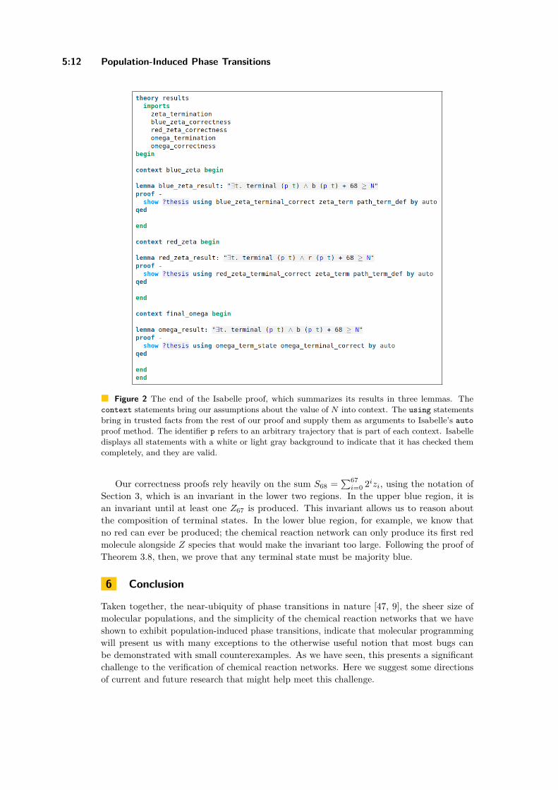
5:12 Population-Induced Phase Transitions
Figure 2 The end of the Isabelle proof, which summarizes its results in three lemmas. Thecontext statements bring our assumptions about the value of N into context. The using statementsbring in trusted facts from the rest of our proof and supply them as arguments to Isabelle’s autoproof method. The identifier p refers to an arbitrary trajectory that is part of each context. Isabelledisplays all statements with a white or light gray background to indicate that it has checked themcompletely, and they are valid.
Our correctness proofs rely heavily on the sum S68 =∑67
i=0 2izi, using the notation ofSection 3, which is an invariant in the lower two regions. In the upper blue region, it isan invariant until at least one Z67 is produced. This invariant allows us to reason aboutthe composition of terminal states. In the lower blue region, for example, we know thatno red can ever be produced; the chemical reaction network can only produce its first redmolecule alongside Z species that would make the invariant too large. Following the proof ofTheorem 3.8, then, we prove that any terminal state must be majority blue.
6 Conclusion
Taken together, the near-ubiquity of phase transitions in nature [47, 9], the sheer size ofmolecular populations, and the simplicity of the chemical reaction networks that we haveshown to exhibit population-induced phase transitions, indicate that molecular programmingwill present us with many exceptions to the otherwise useful notion that most bugs canbe demonstrated with small counterexamples. As we have seen, this presents a significantchallenge to the verification of chemical reaction networks. Here we suggest some directionsof current and future research that might help meet this challenge.

J. I. Lathrop, J. H. Lutz, R. R. Lutz, H.D. Potter, and M.R. Riley 5:13
theory terminimports piptcrn
begin
definition terminal :: state ⇒ bool where terminal s1 = (¬(∃ s2 . K s1 s2 ))definition nonterm :: state ⇒ bool where nonterm s = (¬(terminal s))
definition path-term :: (nat ⇒ state) ⇒ bool where(path-term p) = (∃ t . (terminal (p t)))
definition state-term :: (state ⇒ bool) where(state-term s) = (∀ (p :: (nat ⇒ state)).
((∃ t . ((p t) = s))−→ (path-term p)))
lemma dec-imp-term:fixes f :: state ⇒ natfixes p :: nat ⇒ statefixes c :: natassumes evterm: ((f s) ≤ c) −→ (terminal s)assumes dec: ∀ i . ((¬(terminal (p i))) −→ ((f (p (i + 1 )) < (f (p i)))))
shows path-term pproof −
fix n::nathave ((∃ t . ((f (p t)) ≤ n)) −→ (path-term p))proof (induction n)
case 0then show ?case
using dec gr-implies-not0 path-term-def by blastnext
case (Suc n)then show ?case
by (metis dec le-SucE less-Suc-eq-le path-term-def )qed
then show ?thesis by blast
qed
end
145
Figure 3 This Isabelle code defines a terminal state as a state with no outgoing reactions; K is arelation that encodes which state transitions our reaction set allows. We also show a sample lemmathat helps prove termination: if we identify a countdown expression f and a constant C such thatall states with f < C are terminal, then our system is guaranteed to terminate.
A great deal of creative work has produced a steady scaling up of model checking tolarger and larger state spaces [16, 15, 1, 8, 34, 13]. Perhaps the most hopeful approach fordealing with population-induced phase changes, or with more general population-sensitivebehaviors, is the model checking of parametrized systems [1].
Our results clearly demonstrate the advantage of including theorem proving (by humansand by software) in the verification toolbox for chemical reaction networks and other molecularprogramming languages. This in turn suggests that software proof assistants such as Isabelle[40, 39] be augmented with features to deal more directly with chemical reaction networksand with population-sensitive phenomena. It would also be useful to know how much of suchwork could be carried out with more fully automated theorem provers such as Vampire [25].
Some future programmed molecular applications will be safety-critical, such as in healthdiagnostics and therapeutics. It is likely that evidence that such systems behave as intendedwill be required for certification by regulators prior to deployment. Toward providing suchevidence, Nemouchi et al. have recently shown how a descriptive language for safety casescan be incorporated into Isabelle in order to formalize argument-based safety assurancecases [38].
DNA 26
5:14 Population-Induced Phase Transitions
We conclude with a more focused, theoretical question. Our chemical reaction networkN1 exhibits its phase transition on all trajectories, while N2 exhibits its coupled phasetransitions only on all fair trajectories. Is there a chemical reaction network that achievesN2’s coupled phase transitions on all trajectories?
References
1 Parosh Aziz Abdulla, A. Prasad Sistla, and Muralidhar Talupur. Model checking pa-rameterized systems. In Edmund M. Clarke, Thomas A. Henzinger, Helmut Veith, andRoderick Bloem, editors, Handbook of Model Checking, pages 685–725. Springer, 2018.doi:10.1007/978-3-319-10575-8_21.
2 David F. Anderson and Thomas G. Kurtz. Continuous time Markov chain models for chemicalreaction networks. In Heinz Koeppl, Gianluca Setti, Mario di Bernardo, and Douglas Densmore,editors, Design and Analysis of Biomolecular Circuits, pages 3–42. Springer, 2011.
3 David F. Anderson and Thomas G. Kurtz. Stochastic Analysis of Biochemical Systems.Springer, 2015.
4 Dana Angluin, James Aspnes, and David Eisenstat. A simple population protocol for fastrobust approximate majority. Distributed Computing, 21(2):87–102, 2008.
5 Dana Angluin, James Aspnes, David Eisenstat, and Eric Ruppert. The computational powerof population protocols. Distributed Computing, 20(4):279–304, 2007.
6 Stefan Badelt, Seung Woo Shin, Robert F. Johnson, Qing Dong, Chris Thachuk, and ErikWinfree. A general-purpose CRN-to-DSD compiler with formal verification, optimization,and simulation capabilities. In Proceedings of the 23rd International Conference on DNAComputing and Molecular Programming, Springer, pages 232–248, 2017.
7 Christel Baier and Joost-Pieter Katoen. Principles of Model Checking (Representation andMind Series). The MIT Press, 2008.
8 Luca Bortolussi, Luca Cardelli, Marta Kwiatkowska, and Luca Laurenti. Central limit modelchecking. ACM Trans. Comput. Log., 20(4):19:1–19:35, 2019. doi:10.1145/3331452.
9 Sarah Cannon, Sarah Miracle, and Dana Randall. Phase transitions in random dyadictilings and rectangular dissections. SIAM J. Discret. Math., 32(3):1966–1992, 2018. doi:10.1137/17M1157118.
10 Luca Cardelli and Attila Csikász-Nagy. The cell cycle switch computes approximate majority.Scientific Reports, 2, 2012.
11 Luca Cardelli, Marta Kwiatkowska, and Max Whitby. Chemical reaction network designsfor asynchronous logic circuits. Natural Computing, 17(1):109–130, 2018. doi:10.1007/s11047-017-9665-7.
12 Nathalie Cauchi, Luca Laurenti, Morteza Lahijanian, Alessandro Abate, Marta Kwiatkowska,and Luca Cardelli. Efficiency through uncertainty: scalable formal synthesis for stochastichybrid systems. In Proceedings of the 22nd ACM International Conference on Hybrid Systems:Computation and Control, HSCC 2019, Montreal, QC, Canada, April 16-18, 2019., pages240–251, 2019. doi:10.1145/3302504.3311805.
13 Milan Ceska, Nils Jansen, Sebastian Junges, and Joost-Pieter Katoen. Shepherding hordes ofMarkov chains. In Proceedings of the International Conference on Tools and Algorithms forthe Construction and Analysis of Systems, pages 172–190. Springer, 2019.
14 Yuan-Jyue Chen, Neil Dalchau, Niranjan Srinivas, Andrew Phillips, Luca Cardelli, DavidSoloveichik, and Georg Seelig. Programmable chemical controllers made from DNA. NatureNanotechnology, 8(10):755–762, 2013.
15 Philipp Chrszon, Clemens Dubslaff, Sascha Klüppelholz, and Christel Baier. ProFeat: feature-oriented engineering for family-based probabilistic model checking. Formal Asp. Comput.,30(1):45–75, 2018. doi:10.1007/s00165-017-0432-4.

J. I. Lathrop, J. H. Lutz, R. R. Lutz, H.D. Potter, and M.R. Riley 5:15
16 Edmund M. Clarke, E. Allen Emerson, and Joseph Sifakis. Model checking: algorithmicverification and debugging. Commun. ACM, 52(11):74–84, 2009. doi:10.1145/1592761.1592781.
17 Anne Condon, Monir Hajiaghayi, David G. Kirkpatrick, and Ján Manuch. Simplifying analysesof chemical reaction networks for approximate majority. In Proceedings of the 23rd InternationalConference on DNA Computing and Molecular Programming, pages 188–209. Springer, 2017.
18 Matthew Cook, David Soloveichik, Erik Winfree, and Jehoshua Bruck. Programmability ofchemical reaction networks. In Anne Condon, David Harel, Joost N. Kok, Arto Salomaa, andErik Winfree, editors, Algorithmic Bioprocesses, Natural Computing Series, pages 543–584.Springer, 2009.
19 Shawn M. Douglas, Ido Bachelet, and George M. Church. A logic-gated nanorobot for targetedtransport of molecular payloads. Science, 335(6070):831–834, 2012.
20 Samuel J. Ellis, Titus H. Klinge, James I. Lathrop, Jack H. Lutz, Robyn R. Lutz, Andrew S.Miner, and Hugh D. Potter. Runtime fault detection in programmed molecular systems. ACMTrans. Softw. Eng. Methodol., 28(2):6:1–6:20, 2019. doi:10.1145/3295740.
21 François Fages, Guillaume Le Guludec, Olivier Bournez, and Amaury Pouly. Strong Turingcompleteness of continuous chemical reaction networks and compilation of mixed analog-digitalprograms. In Proceedings of the 15th International Conference on Computational Methods inSystems Biology, pages 108–127. Springer, 2017.
22 David Harel. Effective transformations on infinite trees, with applications to high undecidability,dominoes, and fairness. J. ACM, 33(1):224–248, 1986. doi:10.1145/4904.4993.
23 J. Heath, M. Kwiatkowska, G. Norman, D. Parker, and O. Tymchyshyn. Probabilistic modelchecking of complex biological pathways. In Computational Methods in Systems Biology, pages32–47, Berlin, Heidelberg, 2006. Springer Berlin Heidelberg.
24 Daniel Jackson. Alloy: a language and tool for exploring software designs. Commun. ACM,62(9):66–76, 2019. doi:10.1145/3338843.
25 Laura Kovács and Andrei Voronkov. First-order theorem proving and Vampire. In ComputerAided Verification - 25th International Conference, CAV 2013, Saint Petersburg, Russia, July13-19, 2013. Proceedings, pages 1–35. Springer, 2013. doi:10.1007/978-3-642-39799-8_1.
26 Dexter Kozen. Theory of Computation. Texts in Computer Science. Springer, 2006. doi:10.1007/1-84628-477-5.
27 Thomas G. Kurtz. The relationship between stochastic and deterministic models for chemicalreactions. The Journal of Chemical Physics, 57(7):2976–2978, 1972.
28 Marta Kwiatkowska, Gethin Norman, and David Parker. PRISM 4.0: Verification of proba-bilistic real-time systems. In Proceedings of the 23rd International Conference on ComputerAided Verification, pages 585–591. Springer, 2011.
29 Marta Kwiatkowska and Chris Thachuk. Probabilistic model checking for biology. SoftwareSystems Safety, 36:165–189, 2014.
30 Marta Z. Kwiatkowska. Survey of fairness notions. Information and Software Technology,31(7):371–386, 1989. doi:10.1016/0950-5849(89)90159-6.
31 Matthew R. Lakin, David Parker, Luca Cardelli, Marta Kwiatkowska, and Andrew Phillips.Design and analysis of DNA strand displacement devices using probabilistic model checking.Journal of the Royal Society Interface, 9(72):1470–1485, 2012.
32 Suping Li, Qiao Jiang, Shaoli Liu, Yinlong Zhang, Yanhua Tian, Chen Song, Jing Wang,Yiguo Zou, Gregory J Anderson, Jing-Yan Han, Yung Chang, Yan Liu, Chen Zhang, LiangChen, Guangbiao Zhou, Guangjun Nie, Hao Yan, Baoquan Ding, and Yuliang Zhao. A DNAnanorobot functions as a cancer therapeutic in response to a molecular trigger in vivo. NatureBiotechnology, 36:258, 2018.
33 Xiaowei Liu, Yan Liu, and Hao Yan. Functionalized DNA nanostructures for nanomedicine.Israel Journal of Chemistry, 53(8):555–566, 2013.
34 Alessio Lomuscio and Edoardo Pirovano. A counter abstraction technique for the verificationof probabilistic swarm systems. In Proceedings of the 18th International Conference on
DNA 26

5:16 Population-Induced Phase Transitions
Autonomous Agents and MultiAgent Systems, AAMAS’19, pages 161–169, 2019. URL: http://dl.acm.org/citation.cfm?id=3331689.
35 MATLAB. version 9.7.0 (R2019b, Update 4). The MathWorks Inc., Natick, Massachusetts,2019.
36 Melissa B. Miller and Bonnie L. Bassler. Quorum sensing in bacteria. Annual Review ofMicrobiology, 55(1):165–199, 2001. PMID: 11544353. doi:10.1146/annurev.micro.55.1.165.
37 Cristopher Moore and Stephan Mertens. The Nature of Computation. Oxford University Press,2011.
38 Yakoub Nemouchi, Simon Foster, Mario Gleirscher, and Tim Kelly. Isabelle/SACM: Computer-assisted assurance cases with integrated formal methods. In Proceedings of the 15th Inter-national Conference on Integrated Formal MethodsIFM 2019, pages 379–398. Springer, 2019.doi:10.1007/978-3-030-34968-4_21.
39 Tobias Nipkow and Gerwin Klein. Concrete Semantics–With Isabelle/HOL. Springer, 2014.40 Tobias Nipkow, Lawrence C. Paulson, and Markus Wenzel. Isabelle/HOL, volume 2283 of
Lecture Notes in Computer Science. Springer-Verlag Berlin Heidelberg, 1 edition, 2002.41 Lawrence C. Paulson, Tobias Nipkow, and Makarius Wenzel. From LCF to Isabelle/HOL.
Formal Asp. Comput., 31(6):675–698, 2019. doi:10.1007/s00165-019-00492-1.42 Esteban Pavese, Víctor Braberman, and Sebastián Uchitel. Less is more: Estimating proba-
bilistic rewards over partial system explorations. ACM Transactions on Software Engineeringand Methodology, 25(2):16:1–16:47, 2016.
43 Gerald Pollack and Wei-Chun Chin, editors. Phase Transitions in Cell Biology. Springer,2008.
44 Hamid Ramezani and Hendrik Dietz. Building machines with DNA molecules. Nature ReviewsGenetics, 21(1):5–26, 2020.
45 Dana Randall. Phase transitions in sampling algorithms and the underlying random structures.In Haim Kaplan, editor, Proceedings Scandinavian Symposium and Workshops on AlgorithmTheory SWAT, page 309. Springer, 2010. doi:10.1007/978-3-642-13731-0_29.
46 Dana Randall. Phase Transitions and Emergent Phenomena in Random Structures andAlgorithms (Keynote Talk). In 31st International Symposium on Distributed Computing(DISC 2017), pages 3:1–3:2. Schloss Dagstuhl LZI, 2017. doi:10.4230/LIPIcs.DISC.2017.3.
47 Dana Randall. Statistical Physics and Algorithms (Invited Talk). In Christophe Paul andMarkus Bläser, editors, 37th International Symposium on Theoretical Aspects of ComputerScience (STACS 2020), pages 1:1–1:6. Schloss Dagstuhl LZI, 2020.
48 H. G. Rice. Classes of Recursively Enumerable Sets and Their Decision Problems. PhD thesis,Syracuse University, 1951.
49 H. G. Rice. Classes of recursively enumerable sets and their decision problems.Transactions of the American Mathematical Society, 74:358–366, 1953. doi:10.1090/s0002-9947-1953-0053041-6.
50 Apoorva Sarode, Akshaya Annapragada, Junling Guo, and Samir Mitragotri. Layered self-assemblies for controlled drug delivery: A translational overview. Biomaterials, 242:119929,2020. doi:10.1016/j.biomaterials.2020.119929.
51 David Soloveichik, Matthew Cook, Erik Winfree, and Jehoshua Bruck. Computation withfinite stochastic chemical reaction networks. Natural Computing, 7(4):615–633, 2008.
52 David Soloveichik, Georg Seelig, and Erik Winfree. DNA as a universal substrate for chemicalkinetics. In Proceedings of the 14th International Meeting on DNA Computing, pages 57–69.Springer, 2009.
53 Anupama J. Thubagere, Chris Thachuk, Joseph Berleant, Robert F. Johnson, Diana A.Ardelean, Kevin M. Cherry, and Lulu Qian. Compiler-aided systematic construction of large-scale DNA strand displacement circuits using unpurified components. Nature Communications,8, 2017 .
54 John C. Wooley and Herbert S. Lin. Catalyzing Inquiry at the Interface of Computing andBiology. National Academies Press, 2005.
55 David Yu Zhang and Georg Seelig. Dynamic DNA nanotechnology using strand-displacementreactions. Nature Chemistry, 3(2):103–113, 2011.
J. I. Lathrop, J. H. Lutz, R. R. Lutz, H.D. Potter, and M.R. Riley 5:17
A Proof of Fair Termination Lemma
I Lemma A.1 (fair termination lemma). If a population protocol with a specified initial statehas a terminal trajectory from every reachable state, then all its fair trajectories are terminal.
Proof. Let N be a population protocol with initial state q0, and assume that N has aterminal trajectory from every reachable state. Let τ = (qi | 0 ≤ i < ∞) be an infinitetrajectory of N. It suffices to show that τ is not fair.
For each state q of N, let
Iq = i ∈ N | qi = q. (A.1)
Since N is a population protocol, it has finitely many reachable states, so there is a stateq∗ of N such that the set Iq∗ is infinite. This state q∗ is reachable, so our assumption tellsus that there is a finite trajectory τ∗ = (q∗i | 0 ≤ i < `) of N such that q∗0 = q∗ and q∗`−1 isterminal.
Now Iq∗0
= Iq∗ is infinite and Iq∗`−1
= ∅ (because q∗`−1 is terminal, so it does not appear inthe infinite trajectory τ), so there exists 0 ≤ k < `− 1 such that Iq∗
kis infinite and Iq∗
k+1is
finite. Let q∗∗ = q∗k, and let ρ be the reaction that takes q∗k to q∗k+1. Then ρ is enabled in q∗∗and there exist infinitely many i such that qi = q∗∗ (because Iq∗∗ is infinite), but there areonly finitely many j for which qj = q∗ and ρ occurs at j in τ (because Iq∗
k+1is finite). Hence
τ is not fair. J
DNA 26


ALCH: An Imperative Language for ChemicalReaction Network-Controlled Tile AssemblyTitus H. KlingeDepartment of Mathematics and Computer Science, Drake University, Des Moines, IA, [email protected]
James I. LathropDepartment of Computer Science, Iowa State University, Ames, IA, [email protected]
Sonia MorenoDepartment of Computer Science, Carleton College, Northfield, MN, [email protected]
Hugh D. PotterDepartment of Computer Science, Iowa State University, Ames, IA, [email protected]
Narun K. RamanDepartment of Computer Science, Carleton College, Northfield, MN, [email protected]
Matthew R. RileyDepartment of Computer Science, Iowa State University, Ames, IA, [email protected]
AbstractIn 2015 Schiefer and Winfree introduced the chemical reaction network-controlled tile assembly model(CRN-TAM), a variant of the abstract tile assembly model (aTAM), where tile reactions are mediatedvia non-local chemical signals. In this paper, we introduce ALCH, an imperative programminglanguage for specifying CRN-TAM programs. ALCH contains common features like Boolean variables,conditionals, and loops. It also supports CRN-TAM-specific features such as adding and removingtiles. A unique feature of the language is the branch statement, a nondeterministic control structurethat allows us to query the current state of tile assemblies. We also developed a compiler thattranslates ALCH to the CRN-TAM, and a simulator that simulates and visualizes the self-assemblyof a CRN-TAM program. Using this language, we show that the discrete Sierpinski triangle canbe strictly self-assembled in the CRN-TAM. This solves an open problem that the CRN-TAM iscapable of self-assembling infinite shapes at scale one that the aTAM cannot. ALCH allows us topresent this construction at a high level, abstracting species and reactions into C-like code that issimpler to understand. Our construction utilizes two new CRN-TAM techniques that allow us totackle this open problem. First, it employs the branching feature of ALCH to probe the previouslyplaced tiles of the assembly and detect the presence and absence of tiles. Second, it uses scaffoldingtiles to precisely control tile placement by occluding any undesired binding sites.
2012 ACM Subject Classification Theory of computation → Models of computation
Keywords and phrases Tile assembly, Chemical reaction network, Sierpinski triangle
Digital Object Identifier 10.4230/LIPIcs.DNA.2020.6
Supplementary Material The ALCH compiler and the CRN-TAM simulator, together with examplesand visual illustrations, are available at http://web.cs.iastate.edu/~lamp.
Funding This research was supported in part by National Science Foundation grants 1900716 and1545028.
Acknowledgements We thank the three anonymous reviewers for their helpful comments andsuggestions. We especially thank reviewer 3 for their detailed insights, comments, and suggestions.
© Titus H. Klinge, James I. Lathrop, Sonia Moreno, Hugh D. Potter, Narun K. Raman, and MatthewR. Riley;licensed under Creative Commons License CC-BY
26th International Conference on DNA Computing and Molecular Programming (DNA 26).Editors: Cody Geary and Matthew J. Patitz; Article No. 6; pp. 6:1–6:22
Leibniz International Proceedings in InformaticsSchloss Dagstuhl – Leibniz-Zentrum für Informatik, Dagstuhl Publishing, Germany

6:2 ALCH: An Imperative Language for the CRN-TAM
1 Introduction
Molecular programming is a relatively new field that weaves together biology and computerscience to specify the behavior of molecules at the nanoscale. Early research in the field wassparked in 1982 by Seeman’s pioneering work employing DNA crossover tiles to self-assemblecrystals at the nanoscale [13]. Seeman’s work was later extended by Erik Winfree to includecooperative DNA tile self-assembly to construct more complex shapes and patterns [15].Winfree formalized the abstract tile assembly model (aTAM) in his Ph.D. thesis, wherehe proved it is Turing complete [15]. As a result, the aTAM is considered a programminglanguage for self-assembling two and three-dimensional nanoscale patterns and is still activelyinvestigated today [8, 3, 10, 7].
Another model commonly used to study biomolecular computation is the chemical reactionnetwork (CRN ), which models the interactions of chemical species. The CRN model assumesthe solution is well-mixed, and therefore computations are amorphous and do not relyon geometry or structure. Two common variants of the CRN model are stochastic CRNsand deterministic CRNs. Stochastic CRNs are modeled with discrete species counts, andtheir reactions are probabilistic. In contrast, deterministic CRNs model the species’ statecontinuously with real-valued concentrations governed by a system of autonomous ordinarydifferential equations (ODEs). The law of mass action determines the rates of reactions inboth models. For more information on these models, see [6, 5, 2].
In 2015, Schiefer and Winfree introduced the chemical reaction network-controlled tileassembly model (CRN-TAM ) [11, 12]. Their model combines the amorphous properties ofstochastic CRNs with the spatial self-assembly of complex structures afforded by the aTAM.More specifically, a chemical reaction network interacts with tiles from the aTAM model toexert non-local control over the self-assembly process.
Molecular programming provides a rich field for algorithmic study. However, it is oftentime-consuming and complex to generate algorithmic constructions at the level of chemicalspecies, tiles, or reactions. Recently, Vasić, Soloveichik, and Khurshid introduced CRN++,a high-level language for implementing deterministic CRN programs [14]. The CRN++language provides a toolset for manipulating concentrations as numerical variables, with somesupport for conditionals and loops. This simplifies the development of high-level deterministicCRNs by abstracting away many low-level details. Other such languages exist such as Liekensand Fernando’s Chemical Bare Bones (CBB), a hypothetical chemical implementation ofthe simple but Turing complete Bare Bones programming language [9]. CBB implementsincrement, decrement, and loop instructions using a catalytic particle model in which a singlemultistate particle catalyzes reactions based on its state. However, these languages cannotbe used for CRN-TAM programs, since they have no provision for tile self-assembly.
On the tile self-assembly side, we have seen several forms of abstraction. Becker presentsa geometry-based system for generating shapes in the aTAM [1]. This system allows usersto describe how information and assembly construction propagate along vectors defined inthe physical space of the assembly. Users can then generate an aTAM system by designinga system of vectors and applying a well-defined procedure to convert it into tiles. Dotyand Patitz provide a toolset at a lower level of abstraction, focusing on the connectionsbetween individual tiles and how information is shared across them [4]. Users can definevariables to be transmitted from tile to tile via bond labels and transformation functionsto “modify” those variables within a tile while specifying which sets of tiles can bond withwhich. The provided software then automatically generates an aTAM system. Both of these
T.H. Klinge, J. I. Lathrop, S. Moreno, H.D. Potter, N. K. Raman, and M.R. Riley 6:3
tools focus on the parallel, semi-uncoordinated concept of tile self-assembly typical of aTAMconstructions. In the CRN-TAM, on the other hand, the CRN component allows precisecontrol over which tiles are added and when.
CRN-TAM constructions often rely on sequences of reactions and tile attachments, withsequential execution enforced by associating a chemical species with each reaction in the chain.For this reason, the CRN-TAM is a natural fit for a high-level imperative programminglanguage. In this paper, we present the Algorithmic Language for Chemistry (ALCH),an imperative language for specifying CRN-TAM programs. ALCH targets the specificCRN-TAM design paradigm described above, where the CRN component mediates a strictlycontrolled sequence of tile actions We do not intend ALCH in its current form to be used forhighly parallel aTAM-style constructions.
ALCH is reminiscent of other popular imperative languages, supporting loops andconditionals but omitting numerical computation and function calls. ALCH also containsmany CRN-TAM specific statements that abstract away low-level details of the model’sunderlying semantics while maintaining that statements are executed in sequence. ALCHalso includes a branch statement, a control structure that allows CRN-TAM programs tonondeterministically choose between a finite number of self-assembly paths. We are notaware of any shape that can be constructed in the CRN-TAM but not in ALCH, but wedo not claim that ALCH is as general as the CRN-TAM. We have implemented an ALCHcompiler that translates ALCH code into a proper CRN-TAM program and a simulator thatvisualizes the assembly process of a CRN-TAM program1.
Using ALCH, we demonstrate that the CRN-TAM can construct infinite shapes thatthe aTAM cannot. For example, the discrete Sierpinski triangle is a well-known self-similarfractal that can be weakly self-assembled in the aTAM [15] but cannot be strictly self-assembled [8]. Weak self-assembly allows for “filler” tiles to be used to propagate informationthrough an assembly, whereas strict self-assembly disallows this. We show that the non-localcommunication provided by the CRN-TAM is sufficient to overcome this limitation. UsingALCH, we construct a CRN-TAM program that strictly self-assembles the discrete Sierpinskitriangle. Our construction relies on the ability to add and remove scaffolding tiles andself-assembles the fractal in a natural way, using only localized information contained in thecurrent assembly. We achieve this by using ALCH’s nondeterministic branch feature to probepreviously placed tiles to inform which tiles are placed next. We also use the scaffoldingtiles to occlude any spurious bonding sites, giving precise control over the placement of thenext tile. The construction proceeds in a sequence of stages where each stage successfullyself-assembles a subset of the discrete Sierpinski triangle. After the completion of a stage,all scaffolding tiles are removed, leaving only the Sierpinski triangle tiles. Thus, in thelimit, only the Sierpinski triangle remains, since the scaffolding tiles are removed infinitelyoften. In fact, the ratio of scaffold tiles to Sierpinski triangle tiles approaches zero as theself-assembly process proceeds. The ALCH programming language and simulator simplifiesthe development process and the specification of the CRN-TAM program.
The rest of the paper is organized as follows. Section 2 gives an overview of the CRN-TAM model. Section 3 presents a detailed description of the ALCH programming language,including how each statement is compiled to the CRN-TAM. Section 4 gives an overview ofthe construction for the discrete Sierpinski triangle using the ALCH language, with examplesto illustrate key concepts such as probing using nondeterministic branching. Finally, Section 5discusses some conclusions from this work.
1 The ALCH compiler and the CRN-TAM simulator, together with examples and visual illustrations, areavailable at http://web.cs.iastate.edu/~lamp.
DNA 26

6:4 ALCH: An Imperative Language for the CRN-TAM
2 Preliminaries
We now review the chemical reaction network-controlled tile assembly model (CRN-TAM),which combines the notions of the abstract tile-assembly model (aTAM) [15] and the stochasticchemical reaction network (sCRN) [2]. For a complete introduction to the model, see Schieferand Winfree’s original paper [11].
A tile type is a tuple t = (N,E, S,W ) consisting of four bonds for the north, east, south,and west sides of the tile, respectively. Each bond is a tuple B = (`B , sB) where `B is thelabel and sB is the binding strength which is a non-negative integer. Given a finite set of tiletypes T , an assembly is a partial function α : Z2 99K T that encodes the positions of tiles intwo-dimensional space. If α(i, j) is undefined, then we say that (i, j) is unoccupied in theassembly α. When two adjacent tiles in α have matching bond labels `N on their abuttingsides, we say that they interact with a strength determined by their bond strengths sB .
The literature is unclear about whether it is permissible to have bonds with the samelabel but asymmetric bond strengths; we have made the choice to allow it in this work. Weadopt the prescription that adjacent bonds with the same label have interaction strengths, where s is given by the minimum of the bond strengths. Note that this prescription isphysically plausible; if we view a bond site as an exposed single DNA strand, a strongerbond corresponds to a longer exposed area. We can then choose the base pairs exposed by aweaker bond to be a subset of those exposed by a stronger bond. Our probe mechanism,discussed in a subsequent section, relies on such asymmetric bonds.
The binding graph of an assembly α is a two-dimensional lattice of vertices representingthe tiles of α where two vertices are connected by an undirected edge with weight s if theircorresponding tiles in α interact with strength s. For τ ∈ N, we say that an assembly isτ -stable if the minimum cut of its binding graph is at least τ . We also denote assembliesusing α , and given a tile type t , use t to denote the singleton assembly that consistsof only a single tile of type t placed at the origin. Note that the number of tiles of a giventile type t available in solution is finite but unbounded. This is in contrast to the aTAMwhich assumes an unlimited supply of all tile types throughout the self-assembly process.
A signal species is an abstract molecule type. In contrast to tiles, signal species have nogeometry and are used to facilitate non-local communication in the self-assembly process.Every tile t has a unique removal species t∗, and given a finite set T of tile types, we writeT ∗ = t∗ | t ∈ T to denote the set of all tile removal species of T . Note that the definitionsin Schiefer and Winfree’s papers [11, 12] allow tile removal species to be shared or evenomitted. However, it is convenient for the compiler to always generate tile removal speciesand for them to be unique.
A CRN-TAM program is a tuple P = (S, T,R, τ, I) where T is a finite set of tile types, Sis a finite set of signal species that satisfies T ∗ ⊆ S, τ ∈ N is the temperature, I : S ∪ T → Nis the initial state which specifies how many tiles and signal molecules are initially present,and R is a finite set of reactions that are of the following six types.Signal reactions are of the form X1 + X2 → Y1 + Y2 where X1, X2, Y1, Y2 ∈ S ∪ ε. The
ε symbol denotes the absence of a species, therefore X + ε → Y1 + Y2 is equivalent toX → Y1 + Y2. Since these reactions only consist of signal species, their semantics areidentical to those in the traditional sCRN model. The species on the left-hand-side arecalled reactants and are consumed by the reaction and the species on the right-hand-sideare called products and are produced by the reaction.
Deletion reactions are of the form X + t → Y1 + Y2 where X,Y1, Y2 ∈ S ∪ ε and t ∈ T .These reactions consume a tile, treating it as if it were a signal species. Note, deletionreaction cannot consume tiles bound to the assembly.

T.H. Klinge, J. I. Lathrop, S. Moreno, H.D. Potter, N. K. Raman, and M.R. Riley 6:5
Creation reactions are of the form X1 +X2 → t +Y where X1, X2, Y ∈ S∪ε and t ∈ T .These reactions produce tiles, making them available to interact with assemblies.
Relabelling reactions are of the form X + t1 → Y + t2 where X,Y ∈ S ∪ ε andt1 , t2 ∈ T .
Activation reactions are of the form X + t → t + t∗ where X ∈ S, t ∈ T , and t∗ is the
signal removal species for t . These reactions use tile t to seed a new assembly with t
placed at the origin.Deactivation reactions are of the form t + t∗ → t + Y where t ∈ T , t∗ is the removal
signal for t , and Y ∈ S ∪ ε. These reactions remove the tile t from the singleton
assembly t , thereby deactivating it.
In addition to the reactions above, for each t ∈ T , the following two reactions includedin the set of reactions R.Addition reactions of the form α + t → β + t∗ where β and α are τ−stable
assemblies that differ by one copy of t ∈ T and t∗ ∈ T ∗ is the removal signal for t .
Removal reactions of the form β +t∗ → α + t where again β and α are τ−stable
assemblies that differ by one copy of t ∈ T and t∗ ∈ T ∗ is the removal signal for t .
These reactions can only remove t from β if there is an instance of t that is boundat exactly τ strength.
A CRN-TAM program P is initialized with nonnegative counts of each tile and signalspecies type, according to I. In an execution of P, the reactions above occur in a stochasticsequence. The species or assemblies on the left-hand side of a reaction are the reactants andthose on the right are the products. A reaction is enabled if all of its reactants are present insolution. The subsequent reaction to execute is always chosen randomly from the set of allenabled reactions. The likelihood of choosing a particular reaction is proportional to theproduct of its reactant counts, as with regular stochastic CRNs. If an execution reachesa state where no reactions are enabled, we say that it has terminated. Some CRN-TAMprograms, like the DST construction in this work, do not terminate and continue indefinitely.For more information on the kinetics of the CRN-TAM model, see [12].
The CRN-TAM distinguishes between free tiles in solution and tiles that are part ofactivated assemblies. Free tiles can bond to assemblies, but two free tiles cannot bond together.All tiles come into being as free tiles, including those in the initialization; immediately afterinitialization, then, only signal, creation, deletion, and relabeling reactions are possible.We refer to these reactions as the CRN component of the CRN-TAM program. The CRNcomponent usually serves to coordinate activation, deactivation, addition, and removalreactions and guide tile assembly growth.
In most CRN-TAM constructions, the CRN component is engineered to execute at leastone activation reaction, which creates a new tile assembly so tiles can be added. Tilescreated with creation reactions (or present in solution from the start) can then bond viatheir addition reactions, and potentially later be removed via their removal reactions. Asdiscussed above, a tile can bond at any site on an activated assembly where it would interactwith strength at least τ ; tiles are subject to removal reactions when their interaction strengthdoes not exceed τ . Note that if tile t has a removal signal t∗, then adding t releases t∗,and removing t requires and consumes t∗. This allows the CRN component to interact
DNA 26
6:6 ALCH: An Imperative Language for the CRN-TAM
more precisely with the addition and removal reactions. Some constructions also employ thedeactivation reaction to eliminate existing (singleton) assemblies; unlike in the aTAM, thenumber of concurrent assemblies can increase or decrease over time. The constructions inthis work, however, do not require more than one assembly.
3 The ALCH Programming Language
We present an overview of the features of the ALCH language and its implementation. ALCHis an imperative language with provisions specific to the CRN-TAM model such as the add,remove, activate, and deactivate statements which all take a tile type as a parameter andexecute the corresponding tile actions. ALCH provides high-level features such as conditions,loops, and variable declaration and assignment. To guarantee the proper sequential executionof the code, special line number species are used to track progress through the ALCHprogram. By ensuring that only a single line number species is present at any given time2,the CRN-TAM program can transition from instruction to instruction without introducingany race conditions. At this time, ALCH only supports global variables and three datatypes:bool, BondLabel, and TileSpecies. Variables of type bool may be reassigned throughout thecomputation, but all BondLabel and TileSpecies variables are immutable and final. Oneunique feature of ALCH is the branch statement, which nondeterministically chooses andexecutes multiple independent code blocks of tile addition and removal statements until oneblock finishes execution. Effects from uncompleted blocks are reversed, so only the code fromthe completed block remains. The branch statement also returns a bool associated withthe block that finished successfully. Using branch, it is possible to query the state of tileassemblies without permanently attaching tiles to them. Each block in a branch statement isimplemented as a reversible random walk. As an optimization, blocks can be given differentweights to make them more likely to be chosen at the nondeterministic branch point.
We developed a software compiler in C# that compiles ALCH programs into CRN-TAMprograms. We also developed a simulator for the CRN-TAM that includes the followingtwo extensions to the model which are used only for optimization purposes: (1) it supportsreactions with arbitrary arity, relaxing the CRN-TAM requirement that reactions are atmost bimolecular; (2) it allows any reaction to add, remove, or activate a tile as a side effectand removes the requirement for the specific per-tile add and remove actions. Note that theoutput of the ALCH compiler is strictly compliant with the original CRN-TAM as specifiedin [11]. We have not yet implemented tile deactivation in the simulator.
To demonstrate the expressiveness of ALCH, we will show that the CRN-TAM can strictlyself-assemble an infinite shape at temperature 2 that the aTAM cannot. Consider an infinitestaircase, visualized in Figure 1, where for each k ∈ N, the (2k)th column is 2 + k tiles talland the (2k + 1)th column is one tile tall. The gaps between steps (even-numbered columns)prevent an aTAM program from directly transferring information about the height of onestep to the next. Consequently, all information about the height of steps must be passedalong the base of the assembly; an infinite tileset is required. However, the CRN-TAM canbuild and remove probe tiles that allow the assembly to query the previous column. Wetake advantage of this and show that the CRN-TAM can self-assemble this infinite shape, asshown in Figure 1. Note that we omit the tile and bond declarations but include a graphicalrepresentation of the tile species used in the construction. We also omit the CRN speciesand reactions that ALCH outputs.
2 See Subsection 3.3 for the one exception.

T.H. Klinge, J. I. Lathrop, S. Moreno, H.D. Potter, N. K. Raman, and M.R. Riley 6:7
F f
a
def
a
C r
halt
def
def
A r
a
l
def
B l
def
r
def
NH f
halt
def
a
H h
def
def
halt
NHT f
halt
h
a
HD h
def
h
def
FD fdef
f
def
FT f
a
f
a
bool at_top ;activate C;add H; add B; add A;while ( true )
at_top = branch true ( ) add NHT; add HD; fa l se ( ) add FT; add FD;
;
i f ( at_top ) remove HD; remove NHT;add NH; add H;add B; add A;
else remove FD; remove FT;add F;
Figure 1 An ALCH simulation of the infinite staircase is shown in the upper left. ALCH codefor the staircase is shown on the right-hand side. The definitions of the tile types are not shown butare provided visually with bond labels and strengths in the lower left. On the right-most column ofthe simulation, the FT and FD tiles probe the previous column to detect which tile should beplaced. These probe tiles are temporary and are eventually removed. Chemical species and reactionsof the staircase construction, as output by ALCH, are not shown. Note that the temperature τ ofthe CRN-TAM program is 2.
Intuitively, the self-assembly of the infinite staircase is implemented with a single infiniteloop that repeatedly adds tiles to the assembly. Each execution of the loop begins by probingthe previous column using the branch statement, which nondeterministically attempts toadd the sequence of tiles FT and FD or the sequence of tiles NHT and HD . If thelatter succeeds, the variable at_top is set to true, and if the former succeeds, the variable isset to false. Notice that the true() branch will succeed if and only if the current column isthe same height as the previous column because of the top tile H . The variable at_top isthen used to either (a) finish the current column and initialize the next column or (b) adda single filler tile F and continue with the current column. Using branch to query localstructural information during the assembly is powerful; we employ a similar technique toshow that the discrete Sierpinski triangle can be strictly self-assembled in the CRN-TAM.
We now define each of the language features of the ALCH programming language andexplain how they are implemented in the ALCH compiler. We begin by discussing howvariables are implemented and define some useful notation that we use to specify whatreactions and species are created for each language construct.
The ALCH compiler processes all variable declarations at compile-time. All BondLabeland TileSpecies variables are added to a symbol table for later reference in add, remove,activate, and deactivate statements. Since BondLabel and TileSpecies variables are im-mutable and cannot be reassigned, this simple treatment is sufficient. bool variables areimplemented using two chemical species that are created at compile-time, and we commonlyrefer to them as Boolean flags. A Boolean flag x represents two chemical species (x, x), whereat any given time one of x and x has population 0 and the other has population 1. UnlikeBondLabel and TileSpecies variables, bool variables are mutable and can be reassigned byswitching which species has population 1.
Most ALCH statements are implemented with a set of reactions, and each of theircorresponding reactions includes its line number species as a reactant. When two statementsare executed in sequence, the first statement emits the corresponding line number species
DNA 26
6:8 ALCH: An Imperative Language for the CRN-TAM
of the second when it is finished. This allows the sequential execution of statements andavoids race conditions during the program execution. For statements that return a bool, thecompiler creates a dedicated Boolean flag (x, x) (or, in some cases, links an existing flag) forthat line of code and guarantees that when the statement is executed, the associated flagcontains the correct value.
When defining how each syntactical element of ALCH is implemented, it is convenient touse notation such as <block> to denote compound ALCH statements and expressions. Forexample, in the ALCH program in Figure 1, the if statement and surrounding code can bewritten abstractly as:
<block1>i f (<block2 >)
<block3><block4>
Notice how each <block> represents a sequence of statements. Here <block1> must emit theappropriate line number species for the conditional, and similarly, the if statement mustemit the appropriate line number species for <block4> when it is finished. Since most ofthese language constructs are implemented with chemical species and reactions, the followingnotation is convenient:
Xstart →<block> → Xend (1)
Intuitively this notation means that if the line number species Xstart is produced, then allthe statements corresponding to <block> will be executed. The line number species Xend willbe produced afterward. It is important to note that <block> abstractly represents a sequenceof ALCH instructions, which may themselves use many intermediate line number species.Since some statements return a Boolean flag, we also use T<block> and F<block> to denotethe true and false species of the returned Boolean flag after <block> is executed.
3.1 Boolean Expressions and Variable Assignment
We now discuss how Boolean expressions such as (val1 && val2) || !val3 are evaluated as wellas Boolean assignment statements such as bool a = <block>. We begin with the logicaloperations of negation, conjunction, and disjunction.
Given an abstract Boolean expression represented by <block>, we consider the imple-mentation of the logical negation !<block>. Recall that, at compile-time, <block> is given adual-rail Boolean flag (x, x). To implement negation, we simply need to return the negatedflag (x, x). We handle this at compile-time when we link the ! syntax element with the flagof its child element <block>. Intuitively, the compiler will “cross the wires” of <block>’sBoolean flag when it encounters !<block> so that its output flag is negated. Thus negationdoes not introduce any new species or reactions but rather modifies the output of <block>directly at compile-time so that T<block> and F!<block> are the same species and F<block>and T!<block> are the same species.
To process a conjunction of logical expressions, we evaluate each expression from left toright and immediately return a false Boolean flag if an expression evaluates to false. Onlywhen all expressions have evaluated to true will a true Boolean flag be returned. Below is

T.H. Klinge, J. I. Lathrop, S. Moreno, H.D. Potter, N. K. Raman, and M.R. Riley 6:9
how the conjunction statement <exp1> && <exp2> is implemented:
Xstart →<exp1> → X1 (2)X1 + T<exp1> → X2 + T<exp1> (3)X1 + F<exp1> → Xf + F<exp1> (4)
X2 →<exp2> → X3 (5)X3 + T<exp2> → Xt + T<exp2> (6)X3 + F<exp2> → Xf + F<exp2> (7)
Notice how <exp1> is evaluated first, which emits the line number species X1. The linenumber species together with the species T<exp1> and F<exp1> are used to determinewhether the expression should immediately return false by producing the Xf line numberspecies or continue by producing X2 to start evaluating <exp2>. This process continues untilone expression evaluates to false, or all expressions are true, and the Xt line number speciesis produced. A dedicated Boolean flag for the conditional is needed for output because thecompiler cannot identify any preexisting child element that is guaranteed to hold the correctreturn value after execution. This Boolean flag is added to the CRN at compile-time, alongwith the following reactions to update the flag according to whichever Xt or Xf line numberspecies is produced:
Xt + Tresult → Xend + Tresult (8)Xt + Fresult → Xend + Tresult (9)Xf + Tresult → Xend + Fresult (10)Xf + Fresult → Xend + Fresult (11)
Here the species Tresult and Fresult correspond to the unique Boolean flag generated forthis conjunction statement, and Xend is the line number species that initiates the blockimmediately following the conjunction. We implement logical disjunction in a very similarway: the first time an expression returns true, we immediately return true; if all expressionsreturn false, we return false.
We now describe how Boolean assignment statements such as a = <block> are implemented.To execute this command, we evaluate the right-hand side of the assignment. As discussedabove, <block> has an associated Boolean return flag; when <block> finishes execution, thisflag is guaranteed to hold the correct return value. We then use the flag species as catalyststo direct execution to the lines of code that set the variable a to true or to false accordingly.Below are the reactions that implement the assignment a = <block>:
Xstart →<block> → X1 (12)X1 + T<block> → Xt + T<block> (13)X1 + F<block> → Xf + F<block> (14)
The line number species Xt and Xf encode the Boolean return value of <block>, and thefollowing four reactions copy this result into the global Boolean flag for the variable a:
Xt + Ta → Xend + Ta (15)Xt + Fa → Xend + Ta (16)Xf + Ta → Xend + Fa (17)Xf + Fa → Xend + Fa (18)
DNA 26
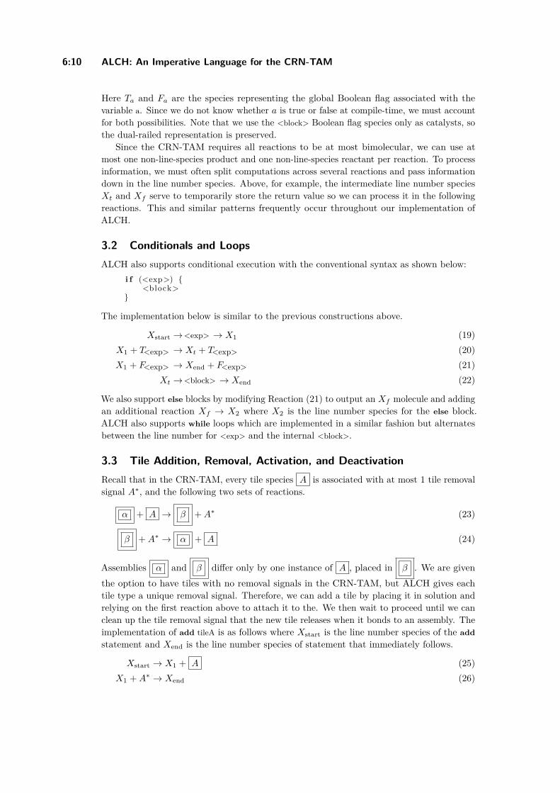
6:10 ALCH: An Imperative Language for the CRN-TAM
Here Ta and Fa are the species representing the global Boolean flag associated with thevariable a. Since we do not know whether a is true or false at compile-time, we must accountfor both possibilities. Note that we use the <block> Boolean flag species only as catalysts, sothe dual-railed representation is preserved.
Since the CRN-TAM requires all reactions to be at most bimolecular, we can use atmost one non-line-species product and one non-line-species reactant per reaction. To processinformation, we must often split computations across several reactions and pass informationdown in the line number species. Above, for example, the intermediate line number speciesXt and Xf serve to temporarily store the return value so we can process it in the followingreactions. This and similar patterns frequently occur throughout our implementation ofALCH.
3.2 Conditionals and LoopsALCH also supports conditional execution with the conventional syntax as shown below:
i f (<exp>) <block>
The implementation below is similar to the previous constructions above.
Xstart →<exp> → X1 (19)X1 + T<exp> → Xt + T<exp> (20)X1 + F<exp> → Xend + F<exp> (21)
Xt →<block> → Xend (22)
We also support else blocks by modifying Reaction (21) to output an Xf molecule and addingan additional reaction Xf → X2 where X2 is the line number species for the else block.ALCH also supports while loops which are implemented in a similar fashion but alternatesbetween the line number for <exp> and the internal <block>.
3.3 Tile Addition, Removal, Activation, and DeactivationRecall that in the CRN-TAM, every tile species A is associated with at most 1 tile removalsignal A∗, and the following two sets of reactions.
α + A → β +A∗ (23)
β +A∗ → α + A (24)
Assemblies α and β differ only by one instance of A , placed in β . We are giventhe option to have tiles with no removal signals in the CRN-TAM, but ALCH gives eachtile type a unique removal signal. Therefore, we can add a tile by placing it in solution andrelying on the first reaction above to attach it to the. We then wait to proceed until we canclean up the tile removal signal that the new tile releases when it bonds to an assembly. Theimplementation of add tileA is as follows where Xstart is the line number species of the addstatement and Xend is the line number species of statement that immediately follows.
Xstart → X1 + A (25)X1 +A∗ → Xend (26)

T.H. Klinge, J. I. Lathrop, S. Moreno, H.D. Potter, N. K. Raman, and M.R. Riley 6:11
The implementation of remove tileA is similar, but it relies on the existence of Reaction (24)discussed earlier:
Xstart → X1 +A∗ (27)
X1 + A → Xend (28)
Assembly activation is more difficult. The CRN-TAM allows only activation reactions ofthe form: X + A → A +A∗. There are two difficulties here. First, it is challenging to
guarantee that A is activated as a new assembly instead of being added to a preexistingassembly. In order for an activation reaction for A to proceed, we must already have A insolution; if A is in solution, we cannot prevent it from bonding to an existing compatiblesite. Instead of guaranteeing this explicitly, we rely on users of ALCH to prevent thesesituations. The second difficulty is that tile activation reactions cannot output a line numberspecies, so we have no easy way of passing execution to the next reaction in our desiredsequence. We handle this issue by producing the desired line number species in advance, asshown in the implementation of activate tileA below.
Xstart → X1 +X3 (29)
X1 → X2 + A (30)
X2 + A → α +A∗ (31)
X3 +A∗ → Xend (32)
Although the line number species X3 is present initially, the last reaction cannot executeuntil the end, when A∗ is also present.
We straightforwardly implement tile deactivation, subject to similar constraints. Insteadof temporarily having two line number species in solution, we temporarily have none as wewait for the deactivation reaction to return one.
3.4 Nondeterministic Branch ConstructWe allow nondeterminism in our language through the branch construct. A branch statementcontains multiple branch paths; a branch path is a sequence of tile addition and removalinstructions collectively associated with a Boolean value. At the start of a branch statement,a program nondeterministically chooses one of the branch paths and begins executing it.Broadly speaking, branch returns the Boolean value of the path that ultimately finishessuccessfully. Each path contains only reversible commands, so if one path is impossible tocomplete, execution will ultimately reverse out of it and proceed down a different path. Sincewe require branch paths to be reversible, we allow only add and remove commands insidebranch paths. It is possible to support additional commands by making other languageconstructs reversible, but for our purposes here, add and remove statements are sufficient.
It is important to note that our notion of reversibility is not complete. For example,suppose we execute add tileA inside a branch path. If this statement is reversed, the systemwill attempt to remove the tile A . However, if there are multiple instances of A bondedto the assembly, it is not guaranteed to remove the same tile added earlier in the branch.Additionally, if we add a tile at a strength greater than τ , we will not be able to remove itwhen attempting to reverse the addition. Any ALCH programmer should exercise cautionwhen using the branch statement to avoid such side effects.
DNA 26

6:12 ALCH: An Imperative Language for the CRN-TAM
r e s u l t = branch true (2 )
add t i l eA ;remove t i l eB ;
fa l se (1 )
remove t i l eC ;
;
Figure 2 Possible execution paths through a branch statement. Instructions associated with trueand instructions associated with false are executed nondeterministically via a random walk. Thebranch statement terminates when one path runs to completion, and it returns the correspondingBoolean flag. The integers inside the parentheses of the true and false branches correspond toweights that bias the random walk.
The branch statement is implemented with a single branch point that can lead to anyone of the branch paths, as shown in Figure 2. From that branch point, we execute onlyone branch path at a time. Since each branch path is reversible, if execution proceeds downa branch that is incapable of completing, it will eventually return to the branch point viarandom walk. When a branch finishes execution, we return the Boolean flag that correspondswith the path that completed.
Consider the following branch statement where <trueblock> and <falseblock> are arbitrarysequences of add and remove statements.
branch true ( ) <trueb lock> fa l se ( ) <f a l s e b l o c k >
The above branch statement is implemented in ALCH with the chemical reactions:
Xstart ↔<trueblock> → Xt (33)Xstart ↔<falseblock> → Xf (34)
A few things should be noted about the above implementation. First, both the <trueblock> and<falseblock> use the same line number species Xstart. Second, those reactions are reversible, asindicated by the bidirectional arrows. Third, once one of the blocks finishes, it is completedwith an irreversible reaction that terminates the branch statement. Fourth, the add andremove commands outside of branch are not reversible; inside branch paths, we modify eachadd and remove command to make them reversible. The reversible implementation for theadd statement is shown below.
X1 ↔ A (35)A∗ ↔ X2 (36)
A reversible remove statement is implemented in a similar way but is not shown.

T.H. Klinge, J. I. Lathrop, S. Moreno, H.D. Potter, N. K. Raman, and M.R. Riley 6:13
The last thing to note about the branch statement is that it returns a Boolean flag.Therefore a dedicated flag must be created at compile-time and be appropriately set afterthe execution is completed. Therefore the following reactions are also needed to set thisBoolean flag.
Xt + Tresult → Xend + Tresult (37)Xt + Fresult → Xend + Tresult (38)Xf + Tresult → Xend + Fresult (39)Xf + Fresult → Xend + Fresult (40)
4 Strict Self-Assembly of the Discrete Sierpinski Triangle
We now present the CRN-TAM construction that strictly self-assembles the discrete Sierpinskitriangle (DST) using ALCH. Our discussion here is complete but brief; see Appendix Afor a more detailed description of our algorithm. To see the complete specification of theconstruction in ALCH, along with a video visualization of the self-assembly, see http://web.cs.iastate.edu/~lamp/.
We begin with an overview of tile types and a brief description of their purpose andthen describe the DST construction algorithm in detail. Since the DST is symmetric aboutthe line f(x) = x, we refer to the two symmetric halves as the lower symmetric triangle(LST) and the upper symmetric triangle (UST). We first discuss the techniques to strictlyself-assemble the LST, which can be easily modified to construct the UST in parallel. Inour construction, it is useful to distinguish between three types of tiles: (1) structural tiles,(2) scaffold tiles, and (3) probe tiles. Structural tiles are permanent and form the DSTitself. Scaffold tiles are used to construct temporary auxiliary structures to facilitate theDST construction. Probe tiles are rapidly added and removed to query existing informationof previously placed structural tiles. To avoid unwanted crosstalk between the symmetrichalves, we duplicate the set of structure tiles into a symmetric group with bonds that areincompatible with the LST tiles. We also differentiate the tile types of even and odd columnsto prevent a partially constructed column from interfering with the construction.
We now discuss the construction for the strict self-assembly of the DST. The first stepin our construction unpacks the initial structure shown in Figure 3a with hard-coded tileactivation and addition statements. This is easily accomplished by adding tiles in a specificorder that avoids ambiguity in placement. After the initial structure tiles are placed, wethen construct the LST column by column, adding structure tiles one-at-a-time, completingeach column before proceeding to the next. We also use a variable to track whether we arecurrently constructing an even or odd column. The process of adding one structure tile at atime is akin to a dot-matrix printer, placing dots of ink one line at a time.
4.1 Scaffold ConstructionWe construct two types of scaffolds. The diagonal scaffold, shown in red in Figure 3, runsalong the diagonal of the DST and provides an anchor for the vertical scaffold, which isshown in cyan. The vertical scaffold covers up potential bond sites that we do not wish tobond to, as illustrated in Figure 3b. The diagonal scaffold is straightforward to construct;before constructing each column, we extend it out by two more tiles. For the vertical scaffold,we must extend it only as far as the base of the DST. We extend the DST base row out by
DNA 26
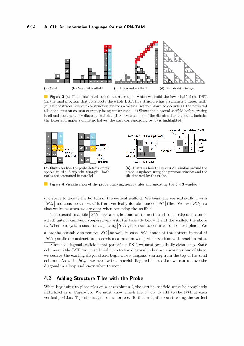
6:14 ALCH: An Imperative Language for the CRN-TAM
(a) Seed. (b) Vertical scaffold. (c) Diagonal scaffold. (d) Sierpinski triangle.
Figure 3 (a) The initial hard-coded structure upon which we build the lower half of the DST.(In the final program that constructs the whole DST, this structure has a symmetric upper half.)(b) Demonstrates how our construction extends a vertical scaffold down to occlude all the potentialtile bond sites on column currently being constructed. (c) Shows the diagonal scaffold before erasingitself and starting a new diagonal scaffold. (d) Shows a section of the Sierpinski triangle that includesthe lower and upper symmetric halves; the part corresponding to (c) is highlighted.
(a) Illustrates how the probe detects emptyspaces in the Sierpinski triangle; bothpaths are attempted in parallel.
(b) Illustrates how the next 3× 3 window around theprobe is updated using the previous window and thetile detected by the probe.
Figure 4 Visualization of the probe querying nearby tiles and updating the 3× 3 window.
one space to denote the bottom of the vertical scaffold. We begin the vertical scaffold withSC0 and construct most of it from vertically double-bonded SC tiles. We use SC0 sothat we know when we are done when removing the scaffold.
The special final tile SCf has a single bond on its north and south edges; it cannotattach until it can bond cooperatively with the base tile below it and the scaffold tile aboveit. When our system succeeds at placing SCf , it knows to continue to the next phase. We
allow the assembly to remove SC as well, in case SC bonds at the bottom instead ofSCf ; scaffold construction proceeds as a random walk, which we bias with reaction rates.
Since the diagonal scaffold is not part of the DST, we must periodically clean it up. Somecolumns in the LST are entirely solid up to the diagonal; when we encounter one of these,we destroy the existing diagonal and begin a new diagonal starting from the top of the solidcolumn. As with SC0 , we start with a special diagonal tile so that we can remove thediagonal in a loop and know when to stop.
4.2 Adding Structure Tiles with the ProbeWhen beginning to place tiles on a new column i, the vertical scaffold must be completelyinitialized as in Figure 3b. We must know which tile, if any to add to the DST at eachvertical position: T-joint, straight connector, etc. To that end, after constructing the vertical
T.H. Klinge, J. I. Lathrop, S. Moreno, H.D. Potter, N. K. Raman, and M.R. Riley 6:15
scaffold, we initialize a 3× 3 Boolean grid, centered on (i, 1), of Boolean flag variables. Thisgrid stores whether those tile positions are occupied in the full DST; note that if we know the3× 3 grid around a position, we know which tile, if any, goes there. The lower six squares areentirely determined by whether i is even or odd; the lowest row of the LST is solid, and thesecond-lowest alternates every space between filled and empty. To determine the upper-leftspace, we use the “probe” to measure whether (i− 1, 2) is filled or empty in column i− 1,which we have already constructed. We do this by nondeterministically attempting to buildtwo structures in parallel, as shown in Figure 4a, and can deduce the value of (i− 1, 2) basedon which one succeeds. If the upper left space (i− 1, 2) is empty, then it is possible to placea tile there; using double-bonded probe tiles, we build south from the scaffold and then westinto the potential empty space. If this construction succeeds, we know that the space isempty. We exploit cooperative bonding to determine if (i − 1, 2) is filled. Structure tilesconnect to each other with double bonds; each structure tile, however, has at least a singlebond on its east edge. Our probe tile, then, has a single bond on its north and west edges.It can bond cooperatively with the scaffold and space (i− 1, 2) only if (i− 1, 2) is filled. Weuse ALCH’s branch structure to nondeterministically try both paths until one succeeds, atwhich point our program knows the upper-left space of the 3× 3 grid. We can then calculatethe upper-center and upper-right spaces using the XOR characterization of the DST.
With the grid filled in, our program can put the correct tile into solution (or skip forwardif no tile is required). All incorrect bond sites in column i are covered by the vertical scaffold,so our tile is guaranteed to bond at the correct location. We must then “slide” the 3× 3 gridone space north (updating the Boolean flags accordingly) to process the next tile site, asillustrated in Figure 4b. The lowest six spaces of the new grid overlap with the old grid, sowe already know them. As during initialization, we can calculate the upper-left space usingthe probe method and the remaining two using XOR. We proceed in this fashion up theentire column until it is completed. Note that when adding tiles in the middle of columni, we must make sure they do not bond into column i+ 1 using bond sites on the part ofcolumn i that we have already constructed. We use even and odd bond types to prevent this;the tiles we add for column i are incompatible with the bond sites in column j.
4.3 Constructing the Upper Symmetric TriangleWe have discussed how to construct the lower symmetric triangle (LST); it is straightforwardto extend this method to the upper symmetric triangle (UST). Since the DST is symmetric, weneed not track any additional information. We generate a symmetric scaffold correspondingto the vertical scaffold discussed above. (Since the diagonal scaffold is off-center, we skipthe symmetric version of SC0 .) When we add a structure tile to the LST, we add itssymmetric version as well. We must also make a straightforward modification to our methodfor finishing off the solid columns (rows in the UST) that signal diagonal scaffold cleanup;see the appendix for details.
5 Conclusion
In this paper, we define ALCH, a programming language for the CRN-TAM, and use it toexhibit a strict self-assembly of the discrete Sierpinski triangle (DST). Our use of ALCH allowsus to conceptualize our construction at the level of imperative tile commands and familiarcontrol structures like conditionals and while loops. Furthermore, since it is impossible tostrictly self-assemble the DST in the aTAM, our construction serves as a proof that theCRN-TAM can strictly self-assemble infinite shapes that the aTAM cannot.
DNA 26

6:16 ALCH: An Imperative Language for the CRN-TAM
We have utilized two new techniques in our DST construction. First, we have used a probemechanism to measure which tiles have been placed, allowing us to derive information fromthe already-constructed system. The probe technique showcases ALCH’s nondeterministicbranch structure, exploring multiple potential executions to find one that can complete. Italso enables us to query the parts of the DST we have already constructed. Second, we haveused a temporary scaffold to occlude undesirable tile bonding sites and precisely controlwhere new tiles are added. Both of these techniques leverage the CRN-TAM’s ability toremove tiles and create temporary structures.
We considered an alternate strategy to construct the DST using a CRN-TAM Turingmachine implementation to control scaffold construction and tile placement. This entailedmaintaining a secondary representation of the partially-constructed DST in the Turingmachine tape, updating and querying it as the construction proceeds. The Turing machinewould likely require unbounded storage to retain the last-constructed column even if itdoes not store the whole DST. On the other hand, our CRN-TAM construction acts as a“transformer,” converting a stream of local data into a stream of tile placements withoutretaining unbounded information. The only part of the DST that we store in a computationalform is the local 3× 3 grid. We update it using the probe mechanism, thereby convertingmeasurements of the existing DST into a bounded representation of the local DST area.
Our second technique, occluding bond sites with a temporary scaffold, is very general;we can apply it to any construction where we have a frontier of potential bond sites andmust bond at a precise one. We expect this technique to be useful in constructing a widevariety of infinite shapes in the CRN-TAM. Our DST construction does not require a Turingmachine, but the full power of CRN-TAM universality is available to use in combination withocclusion scaffolds. We speculate that it is possible to construct every connected recursivelyenumerable subset of Z2 using variants of this technique.
For the current version of ALCH, we have focused on a very sequential programmingmodel. However, the CRN-TAM, allows for potentially massive parallelism via large chemicalpopulations; it would be interesting to explore additional ALCH features that leverage thiscapability. For example, the aTAM tileset design toolkit by Doty and Patitz [4] providesan abstraction for highly-parallel tile assembly. Incorporating a similar tool into ALCHcould enable powerful constructions that combine chemical parallelism with the coordinationcapabilities of ALCH’s imperative framework. More broadly, we speculate that ideas fromclassical concurrent programming are relevant to ALCH as well.
We hope that the tools and techniques presented here will catalyze research into theCRN-TAM and similar hybrid models.
References1 Florent Becker. Pictures worth a thousand tiles, a geometrical programming language for self-
assembly. Theoretical Computer Science, 410(16):1495–1515, 2009. Theory and Applicationsof Tiling. doi:10.1016/j.tcs.2008.12.011.
2 Matthew Cook, David Soloveichik, Erik Winfree, and Jehoshua Bruck. Programmability ofchemical reaction networks. In Algorithmic Bioprocesses, Natural Computing Series, pages543–584. Springer, 2009. doi:10.1007/978-3-540-88869-7_27.
3 David Doty, Jack H Lutz, Matthew J Patitz, Robert T Schweller, Scott M Summers, andDamien Woods. The tile assembly model is intrinsically universal. In Proceedings of the53rd Symposium on Foundations of Computer Science, pages 302–310. IEEE, 2012. doi:10.1109/FOCS.2012.76.
4 David Doty and Matthew J. Patitz. A domain-specific language for programming in the tileassembly model. In Proceedings of the 17th International Conference on DNA Computing

T.H. Klinge, J. I. Lathrop, S. Moreno, H.D. Potter, N. K. Raman, and M.R. Riley 6:17
and Molecular Programming, pages 25–34. Springer Berlin Heidelberg, 2009. doi:10.1007/978-3-642-10604-0_3.
5 Irving Robert Epstein and John Anthony Pojman. An Introduction to Nonlinear ChemicalDynamics: Oscillations, Waves, Patterns, and Chaos. Oxford University Press, 1998. doi:10.1021/ed077p450.1.
6 Martin Feinberg. Foundations of chemical reaction network theory. Springer, 2019. doi:10.1007/978-3-030-03858-8.
7 David Furcy, Scott M. Summers, and Christian Wendlandt. New bounds on the tile complexityof thin rectangles at temperature-1. In Proceedings of the 25rd International Conferenceon DNA Computing and Molecular Programming, pages 100–119. Springer InternationalPublishing, 2019. doi:10.1007/978-3-030-26807-7_6.
8 James I. Lathrop, Jack H. Lutz, and Scott M. Summers. Strict self-assembly of discreteSierpinski triangles. Theoretical Computer Science, 410(4):384–405, 2009. doi:10.1016/j.tcs.2008.09.062.
9 Anthony M. L. Liekens and Chrisantha T. Fernando. Turing complete catalytic particlecomputers. In Advances in Artificial Life, pages 1202–1211. Springer Berlin Heidelberg, 2007.doi:10.1007/978-3-540-74913-4_120.
10 Pierre-Étienne Meunier and Damien Woods. The non-cooperative tile assembly model is notintrinsically universal or capable of bounded Turing machine simulation. In Proceedings of the49th Annual ACM SIGACT Symposium on Theory of Computing, pages 328–341. ACM, 2017.doi:10.1145/3055399.3055446.
11 Nicholas Schiefer and Erik Winfree. Universal computation and optimal construction inthe chemical reaction network-controlled tile assembly model. In Proceedings of the 21stInternational Conference on DNA Computing and Molecular Programming, pages 34–54.Springer International Publishing, 2015. doi:10.1007/978-3-319-21999-8_3.
12 Nicholas Schiefer and Erik Winfree. Time complexity of computation and construction inthe chemical reaction network-controlled tile assembly model. In Proceedings of the 22ndInternational Conference on DNA Computing and Molecular Programming, pages 165–182.Springer International Publishing, 2016. doi:10.1007/978-3-319-43994-5_11.
13 Nadrian C. Seeman. Nucleic acid junctions and lattices. Journal of Theoretical Biology,99(2):237–247, 1982. doi:10.1016/0022-5193(82)90002-9.
14 Marko Vasić, David Soloveichik, and Sarfraz Khurshid. CRN++: Molecular programminglanguage. Natural Computing, pages 1–17, 2020. doi:10.1007/s11047-019-09775-1.
15 Erik Winfree. Algorithmic self-assembly of DNA. PhD thesis, California Institute of Technology,1998. URL: https://resolver.caltech.edu/CaltechETD:etd-05192003-110022.
A Strict DST Construction: Details
We now present a more detailed look into our DST construction in ALCH. We begin with anoverview of tile types and a brief description of their purpose; we then describe the DSTconstruction algorithm in detail.
The DST is symmetric about the line y = x. We refer to the two symmetric halves asthe lower symmetric triangle (LST) and the upper symmetric triangle (UST). We will focuson the LST construction algorithm, as it can be easily modified to construct the UST at thesame time.
A.1 Tile TypesWe distinguish three types of tiles. Structure tiles form the DST itself. Scaffold tiles formsemi-permanent auxiliary scaffolds that enable us to build the DST, and probe tiles are addedand removed quickly to probe the existing structure for useful information. One commonalitybetween all three tile types is the inert bond label, which we use always at strength 0.
DNA 26
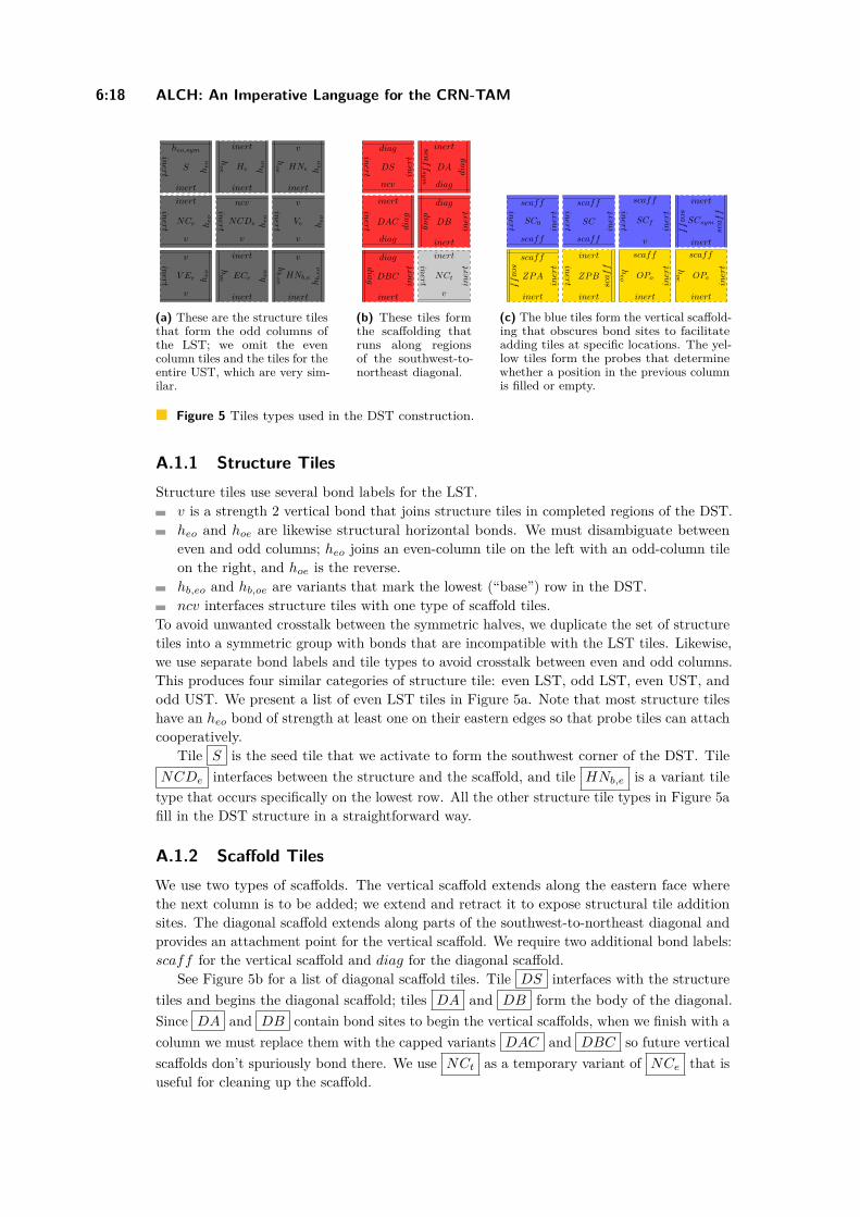
6:18 ALCH: An Imperative Language for the CRN-TAM
S heo
heo,sym
inert
inert
He heo
inert
ho
e
inert
HNe heo
v
ho
e
inert
NCe heo
inert
inert
v
NCDe heo
ncv
inert
v
Ve heo
v
inert
v
V Ee heo
v
inert
v
ECe heo
inert
ho
e
inert
HNb,e
hb,e
o
v
hb,o
e
inert
(a) These are the structure tilesthat form the odd columns ofthe LST; we omit the evencolumn tiles and the tiles for theentire UST, which are very sim-ilar.
DS
inert
diag
inert
ncv
DA
diag
inertscaff
sy
m
diag
DAC
diag
inert
inert
diag
DB
inert
diag
diag
inert
DBC
inert
diag
diag
inert
NCt
inert
inert
inert
v
(b) These tiles formthe scaffolding thatruns along regionsof the southwest-to-northeast diagonal.
SC0
inert
scaff
inert
scaff
SC
inert
scaff
inert
scaff
SCf
inert
scaff
inert
v
SCsym
scaff
inert
scaff
inert
ZPA
inert
scaffscaff
inert
ZPB
scaff
inert
inert
inert
OPo
inert
scaff
heo
inert
OPe
inert
scaff
ho
e
inert
(c) The blue tiles form the vertical scaffold-ing that obscures bond sites to facilitateadding tiles at specific locations. The yel-low tiles form the probes that determinewhether a position in the previous columnis filled or empty.
Figure 5 Tiles types used in the DST construction.
A.1.1 Structure TilesStructure tiles use several bond labels for the LST.
v is a strength 2 vertical bond that joins structure tiles in completed regions of the DST.heo and hoe are likewise structural horizontal bonds. We must disambiguate betweeneven and odd columns; heo joins an even-column tile on the left with an odd-column tileon the right, and hoe is the reverse.hb,eo and hb,oe are variants that mark the lowest (“base”) row in the DST.ncv interfaces structure tiles with one type of scaffold tiles.
To avoid unwanted crosstalk between the symmetric halves, we duplicate the set of structuretiles into a symmetric group with bonds that are incompatible with the LST tiles. Likewise,we use separate bond labels and tile types to avoid crosstalk between even and odd columns.This produces four similar categories of structure tile: even LST, odd LST, even UST, andodd UST. We present a list of even LST tiles in Figure 5a. Note that most structure tileshave an heo bond of strength at least one on their eastern edges so that probe tiles can attachcooperatively.
Tile S is the seed tile that we activate to form the southwest corner of the DST. TileNCDe interfaces between the structure and the scaffold, and tile HNb,e is a variant tiletype that occurs specifically on the lowest row. All the other structure tile types in Figure 5afill in the DST structure in a straightforward way.
A.1.2 Scaffold TilesWe use two types of scaffolds. The vertical scaffold extends along the eastern face wherethe next column is to be added; we extend and retract it to expose structural tile additionsites. The diagonal scaffold extends along parts of the southwest-to-northeast diagonal andprovides an attachment point for the vertical scaffold. We require two additional bond labels:scaff for the vertical scaffold and diag for the diagonal scaffold.
See Figure 5b for a list of diagonal scaffold tiles. Tile DS interfaces with the structuretiles and begins the diagonal scaffold; tiles DA and DB form the body of the diagonal.Since DA and DB contain bond sites to begin the vertical scaffolds, when we finish with acolumn we must replace them with the capped variants DAC and DBC so future verticalscaffolds don’t spuriously bond there. We use NCt as a temporary variant of NCe that isuseful for cleaning up the scaffold.

T.H. Klinge, J. I. Lathrop, S. Moreno, H.D. Potter, N. K. Raman, and M.R. Riley 6:19
We present a list of vertical scaffold tiles in Figure 5c. Tiles SC and SCsym form the
body of the vertical and symmetric horizontal scaffolds. We use SC0 and SCf at thebeginning and end of the LST vertical scaffold so that we can identify when we are doneadding and removing it; since we know this information from the LST, we don’t requirecorresponding symmetric tile species.
A.1.3 Probe TilesWhen constructing a new column, we use a probe mechanism to determine whether specificrows in the last constructed column contain structure tiles; this allows us to use XOR toreconstruct the DST with constant information stored in chemical species counts. We haveseparate probe mechanisms to detect “zeros” (empty positions) and “ones” (filled positions).See Figure 5c for a list of probe tiles.
A.2 InitializationWe now begin our discussion of the DST construction algorithm. First, we prepare thestructure shown in Figure 3a, using a straightforward series of tile additions that do notresult in ambiguity. We also initialize to odd the flag that tracks whether we are in an evenor an odd column.
We face two challenges when constructing the rest of the triangle:We must add each tile in the correct location, instead of any of a potentially unboundednumber of incorrect locations.At each position, we must determine which tile to add, if any; i.e., we must know whetherto add nothing, ECe , HNe , etc.
We solve the first problem by tracking the tile positions around the tile position in question.To solve the second problem, we extend a scaffold of tiles to occlude all unintended bondsites.
To begin, we add the diagonal scaffold tile DS above NCDe ; this will be the start ofour occluding scaffold. Immediately after DS is added, we enter a loop construct in ouralgorithm. We will refer to this loop as the outer loop; each outer loop iteration constructsanother column of the LST.
A.3 Outer Loop
A.3.1 Initialization: building the scaffoldInside the loop, we must first build out the scaffold. We add DA and DB to DS , andwe extend the base row with Hb,o (or HNb,e in an even row). Since we have a tile set
specifically for constructing the base layer, we don’t need to worry about adding Hb,o inthe wrong row.
Now, we construct the vertical scaffold down from DB to produce a structure like theone shown in Fig 3b. We add SC0 first so that when we remove it again we will know wehave reached the top; as discussed below, SCf is a mechanism to detect the bottom row.
We then add SC until we reach the bottom row. Since we have added Hb,o extending
out, we cannot add SC at row 0 or lower. We must detect when we reach the bottom,however, so we can stop attempting to add SC and continue with the rest of the program.
DNA 26

6:20 ALCH: An Imperative Language for the CRN-TAM
Whenever we attempt to add SC , we also attempt to add SCf in parallel using the
branch structure. Recall that Hb,o always has a bond site on its north edge; since SCf
has single bonds on its north and south edges and must bond at strength 2, it can only bondin row 1 between Hb,o to the south and SC to the north.
It may be that SC bonds in row 1 instead of SCf ; we always add SC reversibly so
that if this happens the program can proceed (and can only proceed) by removing SC . Inthis way we have as many chances as we need to add SCf and continue with the program.
We attempt to add SC in one branch and SCf in another; the return value tells uswhether we have finished adding the scaffold.
A.3.2 Guaranteeing correct added tile positionWe can now remove the vertical scaffold row by row, exposing only one tile addition site at atime. There are two types of addition sites: north and east edges of preexisting tiles. Weclaim that when we add a new structure tile, at most one potential bond site is exposed, sothe tile is added unambiguously.
Recall that we have separate bond types for even and odd columns; an odd-columnstructure tile cannot bond to the east side of another odd-column structure tile, and likewisewith even columns. If we are building column i, then, we don’t need to worry aboutunintended bonding in column i+ 1. In column i itself, the region above our intended bondsite is covered by vertical scaffold tiles and is therefore not a concern. In the region belowour intended bond site, all viable bond sites have already been taken up. We can thereforeguarantee that we can always add the next DST structure tile unambiguously.
A.3.3 Choosing the correct tileNow that we can guarantee that tiles are added at the correct position, we must determinewhich tile to add and whether or not to add one at all.
We store a 3 × 3 “window” of boolean flags around the tile position where we willpotentially add a tile, as shown in Fig. 4b. Each flag is true or false based on whether thecorresponding position in the DST is full or empty. Note that if we possess this information,it is easy to determine whether we must add the center tile, and, if so, which tile we mustadd.
If we are constructing column i, we have added the first tile Hb,o or HNb,e at position(i, 0). We will therefore initialize the 3× 3 grid centered on (i, 1), which is the next potentialtile position to fill. The bottom row is always filled in all three positions by the base row, sowe can initialize the lower three flags to true. The second row in the DST always alternatesbetween full and empty, so we need to set either the center flag or the center-left andcenter-right flags to true depending on whether we are building an odd or an even column.Since we track this information, we can easily initialize the middle row.
We do not immediately have enough information to initialize the upper tiles. Recall,however, that the DST can be characterized as a cellular automaton based on the XORrelation ⊕:
DST [x, y]↔ DST [x− 1, y]⊕DST [x, y − 1]. (41)
Therefore if we could somehow measure the upper-left tile, we could calculate the upper-centerand upper-right tiles.
T.H. Klinge, J. I. Lathrop, S. Moreno, H.D. Potter, N. K. Raman, and M.R. Riley 6:21
We can measure the upper-left tile (i− 1, 2) using the branch construct. We require twoseries of tile additions: one that is only possible if (i− 1, 2) is empty, and one that is onlypossible if it contains a tile.
If (i − 1, 2) is empty, we can add a “zero probe” tile into that location; we thereforeattempt to add such a tile, first building ZPA down from the scaffold and then attemptingto build ZPB at (i− 1, 2). See Fig. 4a for an illustration.
Recall that all structural tiles have an east bond site of strength at least one. We thereforeattempt in parallel to add a “one probe” OP with strength-one north and west bond sites.If there is a structural tile in (i− 1, 2), then the one probe can bond cooperatively with itand the vertical scaffold, as shown in Fig. 4a.
We perform these attempts in parallel using the branch construct. It is possible thatZPA will bond when (i− 1, 2) is full. Since we add ZPA reversibly, this is not a problem;the program can only proceed by removing ZPA , and OP then has another chance tobond. It is clear, then, that only the correct branch can fully complete. When it does, thebranch statement returns the correct value of (i− 1, 2).
Once we know (i− 1, 2), we can calculate the upper-center tile value in our 3× 3 windowusing the XOR characterization of the DST. We can then similarly calculate the upper-righttile; that completes the grid, and we can add the appropriate tile into the exposed bond siteor skip it if no tile is required.
We must then adjust the grid so it is centered on (i, 2) instead of (i, 1). Note that thelower two rows of the new grid must be the same as the upper two rows of the old grid,which we have already calculated and stored. We therefore need to calculate only the toprow. We can measure (i − 1, 3) in the same way we measured (i − 1, 2); this allows us tocalculate the new top row the same way we calculated the old top row. We can then continueadding or skipping tiles and sliding the grid upwards iteratively as we construct the column;one sliding iteration is shown in Fig. 4b.
At some point we will attempt to remove SC and instead remove SC0 ; we detect thiswith the branch construct and terminate the column loop. This also signals the end of theouter loop. We remove DB and replace it with DBC so that new SC and SC0 tilescan’t bond there and restart the outer loop.
A.4 Cleaning Up the DiagonalAs we build additional columns, we extend the diagonal scaffold along the diagonal of theDST; since it is not part of the DST, we must periodically remove it to “clean up” ourconstruction.
At every horizontal coordinate that is a power of 2, the DST contains a column of filledcells that extends all the way from the baseline to the diagonal, as shown in Fig 3c. We candetect this in our program by inspecting the state of the 3× 3 grid when we remove SC0 ;if we have just completed a column of filled cells, we clean up the diagonal in the region tothe left of the completed column.
We began the diagonal scaffold with a special tile DS , just as we begin the verticalscaffolds with SC0 . We can therefore remove DA and DBC repeatedly until we caninstead remove DS with the branch construct. When we remove DS , we have cleaned upthe scaffold.
Recall that there is a specific tile NCDe with a north bond site that allows the diagonalscaffold to connect. On the old column that supported the diagonal scaffold, we must replaceNCDe with NCe ; otherwise when we attempt to add the diagonal scaffold, it might bond
DNA 26

6:22 ALCH: An Imperative Language for the CRN-TAM
on the old column instead of the new one. We must also ensure that NCDe is at the topof the new column. To facilitate this swap without risking an unintended tile placement, weplace a new tile species NCt as a temporary cap on the new column. At the end of thisprocess, all tile positions to the left of the new column correctly match the LST, with noexcess scaffold. Since we repeat this process iteratively at farther and farther positions, weare strongly constructing the LST.
A.5 Constructing the Upper Symmetric TriangleWe have shown a construction of the lower symmetric triangle (LST) of the DST. Wecan construct the upper symmetric triangle (UST) at the same time using a very similarmechanism. There is no need to calculate the 3× 3 grid for the UST, as we already know itssymmetric version for the LST.
We duplicate the tileset that we used to construct the LST so that there is no tileplacement ambiguity between symmetric halves. With a few exceptions, discussed below,whenever we add or remove a vertical scaffold or structure tile in the LST, we also add orremove the symmetric tile in the UST. Also, since the horizontal scaffold bonds onto DA ,we must replace DA with DAC at the end of the outer loop.
The diagonal scaffold is not entirely symmetric across the diagonal axis, so we must makeseveral adjustments. First, since the diagonal scaffold occupies the spaces where SC0 wouldgo in the UST, we do not add a symmetric SC0 ; we attach the horizontal scaffold directlyonto the diagonal scaffold. We rely on the SC0 tile in the LST to inform horizontal scaffoldremoval. Second, every power-of-two row in the UST intersects with the diagonal at one gridpoint; we fill in that grid point manually every time we clean up a section of the diagonalscaffold.
With these modifications, our ALCH program strongly constructs the full DST in theCRN-TAM.
Implementing Non-Equilibrium Networks withActive Circuits of Duplex CatalystsAntti LankinenDepartment of Bioengineering, Imperial College London, [email protected]
Ismael Mullor RuizDepartment of Bioengineering and Imperial College Centre for Synthetic Biology, Imperial CollegeLondon, [email protected]
Thomas E. OuldridgeDepartment of Bioengineering and Imperial College Centre for Synthetic Biology, Imperial CollegeLondon, [email protected]
AbstractDNA strand displacement (DSD) reactions have been used to construct chemical reaction networksin which species act catalytically at the level of the overall stoichiometry of reactions. These effectivecatalytic reactions are typically realised through one or more of the following: many-stranded gatecomplexes to coordinate the catalysis, indirect interaction between the catalyst and its substrate,and the recovery of a distinct “catalyst” strand from the one that triggered the reaction. Thesefacts make emulation of the out-of-equilibrium catalytic circuitry of living cells more difficult. Here,we propose a new framework for constructing catalytic DSD networks: Active Circuits of DuplexCatalysts (ACDC). ACDC components are all double-stranded complexes, with reactions occurringthrough 4-way strand exchange. Catalysts directly bind to their substrates, and the “identity” strandof the catalyst recovered at the end of a reaction is the same molecule as the one that initiated it. Weanalyse the capability of the framework to implement catalytic circuits analogous to phosphorylationnetworks in living cells. We also propose two methods of systematically introducing mismatcheswithin DNA strands to avoid leak reactions and introduce driving through net base pair formation.We then combine these results into a compiler to automate the process of designing DNA strandsthat realise any catalytic network allowed by our framework.
2012 ACM Subject Classification Hardware → Biology-related information processing
Keywords and phrases DNA strand displacement, Catalysis, Information-processing networks
Digital Object Identifier 10.4230/LIPIcs.DNA.2020.7
Supplementary Material A compiler to generate optimal sequences for each strand in any allowedcatalytic network is available at https://zenodo.org/record/3948343.
1 Introduction
DNA is an attractive engineering material due to the high specificity of Watson-Crickbase pairing and well-characterised thermodynamics of DNA hybridisation [13,40], whichgive DNA the most predictable and programmable interactions of any natural or syntheticmolecule [43]. DNA computing involves exploiting these properties to assemble computationaldevices made of DNA. The computational circuits are typically realised using DNA stranddisplacement (DSD) reactions, in which sections of DNA strands called domains with partialor full complementarity hybridise, displacing one or more previously hybridised strands inthe process [55]. DSD is initiated by the binding of short complementary sequences calledtoeholds. It is helpful to divide DSD reactions into a few common reaction steps, including:
© Antti Lankinen, Ismael Mullor Ruiz, and Thomas E. Ouldridge;licensed under Creative Commons License CC-BY
26th International Conference on DNA Computing and Molecular Programming (DNA 26).Editors: Cody Geary and Matthew J. Patitz; Article No. 7; pp. 7:1–7:25
Leibniz International Proceedings in InformaticsSchloss Dagstuhl – Leibniz-Zentrum für Informatik, Dagstuhl Publishing, Germany

7:2 Active Circuits of Duplex Catalysts
binding, unbinding, and three- or four-way strand displacement and branch migration, shownin Figure 1. DSD is an attractive scheme for computation as it can be used as a mediumin which to realise chemical reaction networks (CRNs) [44], which provide an abstractionof systems exhibiting mass-action chemical kinetics and have been shown to be Turingcomplete [27]. DSD is then Turing complete as well [34,52]. DSD has been used to construct,for example, logic circuits [35,42], artificial neural networks [9,17,38], dynamical systems [46],catalytic networks [8,36,56], and other computational devices [1,53]. To facilitate testing andrealisation of DSD systems, domain-level design tools [23, 45] as well as domain-to-sequencetranslation [54] software have been introduced.
While DNA nanotechnology is concerned with using DNA as a non-biological material,a key goal of DNA nanotechnology is the imitation and augmentation of cellular systems.It is therefore worth considering how these natural systems typically perform computationand information processing. One ubiquitous biological paradigm for signal propagationand processing is the catalytic activation network, as exemplified by kinases [20, 28, 29].Kinases are catalysts that modify substrates by phosphorylation and consume ATP inthe process. These substrates can be, for example, transcription factors, but can also bekinases themselves that are either activated or deactivated by phosphorylation. The oppositefunction, dephosphorylation, is performed by phosphatases [4]. The emergent catalyticnetwork then performs information propagation or computation by converting species, kinasesand phosphatases, between their active and passive states. Kinase cascades are featured inmany key biological functions, such as cellular growth, adhesion, and differentiation [28,51]and long-term potentiation [47].
Most catalytic networks - including many with a simple topology and a constant steadystate, such as a a single kinase and phosphatase species competing to activate/deactivatea substrate - operate out of equilibrium and consume fuel even in their steady state. Thisfuel-consuming, non-equilibrium behaviour is vital in allowing them to perform functions suchas signal splitting, amplification, time integration and insulation [5, 12,18,30,31]. Moreover,since the key molecular species are recovered rather than consumed by reactions, catalyticnetworks can operate continuously, responding to stimuli as they change over time - unlikemany architectures for DSD-based computation and information processing that operate byallowing the key components to be consumed [1, 9, 38]. This ability to operate continuouslyis invaluable in autonomous environments such as living cells.
In this work, we propose a minimal mechanism for implementing reaction networks ofmolecules that exist in catalytically active and inactive states, a simple abstraction of naturalkinase networks. In these catalytic activation networks, we implement arbitrary activationreactions of the form Aon + Boff +
∑i Fi → Aon + Bon +
∑i Wi, i ∈ 1, 2, 3.... Here, the
catalyst A in its active state Aon drives B between its inactive and active states (Boff , Bon) bythe conversion of one or more fuel molecules Fi into waste Wi. Equivalent deactivationreactions in which an active catalyst deactivates a substrate are also considered.
The rest of this paper is organised as follows. In Section 2, we propose and motivatethe concept of a direct bimolecular catalytic reaction and consider the necessary conditionsfor DSD species that are able to perform such reactions. Section 3 introduces a novel DSDframework to implement these reactions, and its computational properties are analysedin Section 4. Based on these findings, we propose a systematic method of introducingmismatched base pairs within species in our framework to improve its function in Section 5.We combine our findings and propositions into a software to automate the sequence-leveldesign of any CRN that is realisable within our framework, and detail this software in Section6. In Section 7, we discuss our framework, findings, and future work. We conclude the paperin Section 8.
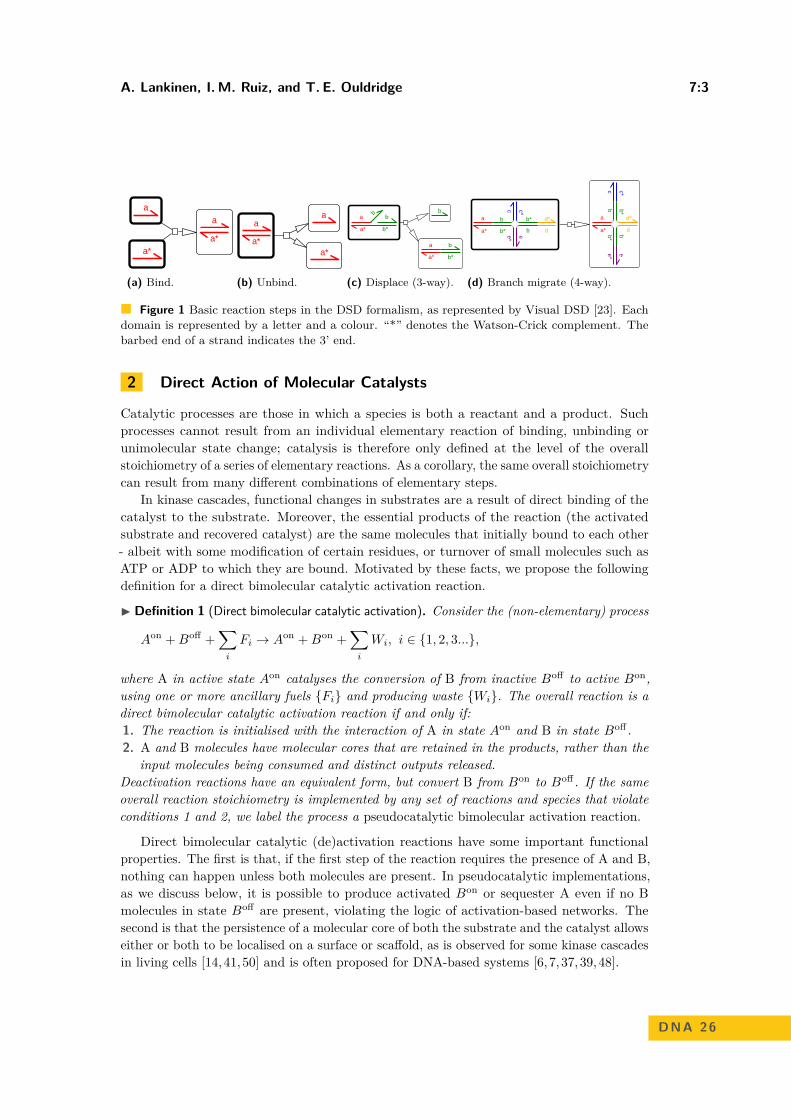
A. Lankinen, I.M. Ruiz, and T. E. Ouldridge 7:3
a
a*
a
a*
(a) Bind.
a
a*
a
a*
(b) Unbind.
b
b
b*a*
a
a
a*
b
b
b*
(c) Displace (3-way).
b*a*
ba
ee*
b* d*
b d
c*c
a*
a
be
b*e*
d*
d
c*b*
cb
(d) Branch migrate (4-way).
Figure 1 Basic reaction steps in the DSD formalism, as represented by Visual DSD [23]. Eachdomain is represented by a letter and a colour. “*” denotes the Watson-Crick complement. Thebarbed end of a strand indicates the 3’ end.
2 Direct Action of Molecular Catalysts
Catalytic processes are those in which a species is both a reactant and a product. Suchprocesses cannot result from an individual elementary reaction of binding, unbinding orunimolecular state change; catalysis is therefore only defined at the level of the overallstoichiometry of a series of elementary reactions. As a corollary, the same overall stoichiometrycan result from many different combinations of elementary steps.
In kinase cascades, functional changes in substrates are a result of direct binding of thecatalyst to the substrate. Moreover, the essential products of the reaction (the activatedsubstrate and recovered catalyst) are the same molecules that initially bound to each other- albeit with some modification of certain residues, or turnover of small molecules such asATP or ADP to which they are bound. Motivated by these facts, we propose the followingdefinition for a direct bimolecular catalytic activation reaction.
I Definition 1 (Direct bimolecular catalytic activation). Consider the (non-elementary) process
Aon + Boff +∑
i
Fi → Aon + Bon +∑
i
Wi, i ∈ 1, 2, 3...,
where A in active state Aon catalyses the conversion of B from inactive Boff to active Bon,using one or more ancillary fuels Fi and producing waste Wi. The overall reaction is adirect bimolecular catalytic activation reaction if and only if:1. The reaction is initialised with the interaction of A in state Aon and B in state Boff .2. A and B molecules have molecular cores that are retained in the products, rather than the
input molecules being consumed and distinct outputs released.Deactivation reactions have an equivalent form, but convert B from Bon to Boff . If the sameoverall reaction stoichiometry is implemented by any set of reactions and species that violateconditions 1 and 2, we label the process a pseudocatalytic bimolecular activation reaction.
Direct bimolecular catalytic (de)activation reactions have some important functionalproperties. The first is that, if the first step of the reaction requires the presence of A and B,nothing can happen unless both molecules are present. In pseudocatalytic implementations,as we discuss below, it is possible to produce activated Bon or sequester A even if no Bmolecules in state Boff are present, violating the logic of activation-based networks. Thesecond is that the persistence of a molecular core of both the substrate and the catalyst allowseither or both to be localised on a surface or scaffold, as is observed for some kinase cascadesin living cells [14, 41,50] and is often proposed for DNA-based systems [6, 7, 37,39,48].
DNA 26

7:4 Active Circuits of Duplex Catalysts
c b
c* b*
e
b*
Gate:Output
c b e
Output
c b
c* b*
d
b*
Gate:Fuel
c* b*
c b
b*
a
Gate:Input
c b d
Fuel
a b c
Input
Figure 2 Catalytic reaction using a seesaw gate [19, 36]. Reactants are shown in bold boxes; theinput acts pseudocatalytically to “convert” the fuel into an output, with ancillary gate complexesconsumed and produced. Each compound reaction is illustrated by a small square, and consists ofsequential bind, displace, and unbind reactions. All reactions are reversible; open arrows indicatereactions proceeding forwards, and closed arrows by reactions proceeding backwards.
A number of DNA computing frameworks have been developed to implement reactionsof the stoichiometry of Definition 1. The simplest, illustrated in Figure 2 (a), involves atwo-step seesaw gate [19,36]. An input molecule (representing A in state Aon in Definition1) binds to a gate-output complex (F ), releasing the output (B in state Bon). The inputis then displaced by a molecule conventionally described as the fuel, but fulfilling the roleof B in state Boff from Definition 1 in the context of catalysis, recovering A in state Aon
and generating a waste duplex (W ). Although the A molecule recovered at the end of theprocess is the same one that initiated the process, the strands representing Boff and Bon
molecules are distinct and the reaction is not initiated by the binding of A and B; it istherefore pseudocatalytic.
This pseudocatalysis can have important consequences. If a small quantity of input thestrand representing Aon is added to a solution containing the gate-output complex F butno strand representing Boff , a large fraction of the Aon strand will be sequestered and acorresponding amount of the Bon strand produced. This sequestration of A and productionof activated B from nothing violates the logic of ideal catalytic activation networks.
More complex strategies to implement reactions of the stoichiometry of Definition 1 usingDSD exist [8, 34]. These approaches rely on the catalyst and substrate (Aon and Boff fromDefinition 1) interacting with a gate, rather than binding to each other, and the recoveredcatalyst and product are separate strands - the reactions are therefore pseudocatalytic. Incertain limits, these strategies can approximate a mass-action dependence of reaction rateson the concentrations of Aon and Boff [8, 33], providing a better approximation to the logicof ideal catalytic activation circuits than the simple seesaw motif. The price, however, isthe need to construct large multi-stranded gate complexes to facilitate the reaction; thecomplexity of these motifs is a major barrier to implementing such systems in autonomoussetting such as living cells. Moreover, localising catalysts and substrates to a scaffold orsurface remains challenging when the molecules themselves are not recovered.
We now consider how to design minimal DSD-based units that implement direct bimolecu-lar catalytic (de)activation in catalytic activation networks. If the core of the substratespecies B must be retained in both Boff and Bon, Boff and Bon cannot simply be two strandswith a slightly different sequence. Instead, Boff and Bon must either be distinct complexesof strands, in which at least one strand is common, have different secondary structure withina single strand, or both. To avoid complexities in balancing the thermodynamics of hairpinloop formation with bimolecular association, and suppressing the kinetics of unimolecularrearrangement, we do not pursue the possibility of engineering metastable secondary structure
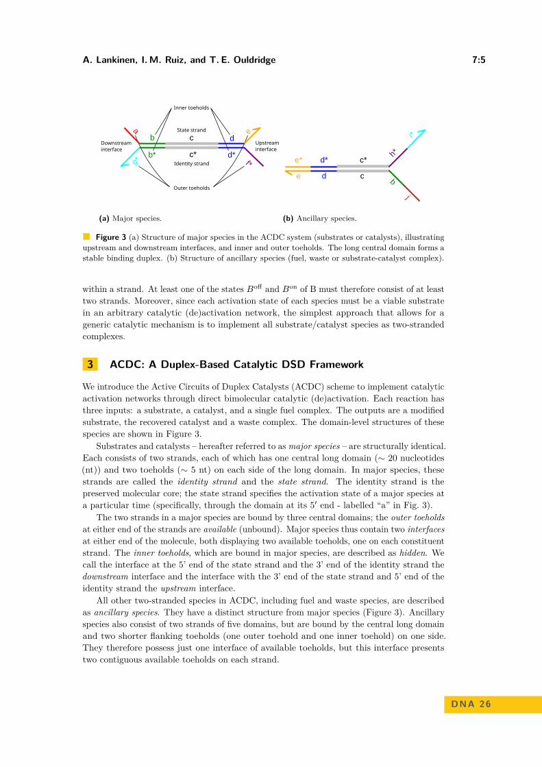
A. Lankinen, I.M. Ruiz, and T. E. Ouldridge 7:5
c*b*
cbg*
d*
d
f*
ea State strand
Identity strand
Upstreaminterface
Downstreaminterface
Inner toeholds
Outer toeholds
(a) Major species.
e* d* c*
e d c
h*
i*
b
j
(b) Ancillary species.
Figure 3 (a) Structure of major species in the ACDC system (substrates or catalysts), illustratingupstream and downstream interfaces, and inner and outer toeholds. The long central domain forms astable binding duplex. (b) Structure of ancillary species (fuel, waste or substrate-catalyst complex).
within a strand. At least one of the states Boff and Bon of B must therefore consist of at leasttwo strands. Moreover, since each activation state of each species must be a viable substratein an arbitrary catalytic (de)activation network, the simplest approach that allows for ageneric catalytic mechanism is to implement all substrate/catalyst species as two-strandedcomplexes.
3 ACDC: A Duplex-Based Catalytic DSD Framework
We introduce the Active Circuits of Duplex Catalysts (ACDC) scheme to implement catalyticactivation networks through direct bimolecular catalytic (de)activation. Each reaction hasthree inputs: a substrate, a catalyst, and a single fuel complex. The outputs are a modifiedsubstrate, the recovered catalyst and a waste complex. The domain-level structures of thesespecies are shown in Figure 3.
Substrates and catalysts – hereafter referred to as major species – are structurally identical.Each consists of two strands, each of which has one central long domain (∼ 20 nucleotides(nt)) and two toeholds (∼ 5 nt) on each side of the long domain. In major species, thesestrands are called the identity strand and the state strand. The identity strand is thepreserved molecular core; the state strand specifies the activation state of a major species ata particular time (specifically, through the domain at its 5′ end - labelled “a” in Fig. 3).
The two strands in a major species are bound by three central domains; the outer toeholdsat either end of the strands are available (unbound). Major species thus contain two interfacesat either end of the molecule, both displaying two available toeholds, one on each constituentstrand. The inner toeholds, which are bound in major species, are described as hidden. Wecall the interface at the 5’ end of the state strand and the 3’ end of the identity strand thedownstream interface and the interface with the 3’ end of the state strand and 5’ end of theidentity strand the upstream interface.
All other two-stranded species in ACDC, including fuel and waste species, are describedas ancillary species. They have a distinct structure from major species (Figure 3). Ancillaryspecies also consist of two strands of five domains, but are bound by the central long domainand two shorter flanking toeholds (one outer toehold and one inner toehold) on one side.They therefore possess just one interface of available toeholds, but this interface presentstwo contiguous available toeholds on each strand.
DNA 26

7:6 Active Circuits of Duplex Catalysts
The catalytic reaction of a single ACDC unit proceeds as shown in Figure 4. Thedownstream interface of the catalyst A in state Aon and upstream interface of the substrateB in state Boff bind together through recognition of all four available toeholds in the relevantinterfaces. The resultant complex undergoes a 4-way branch migration, with the base pairsbetween the state and identity strand of the substrate and catalyst being exchanged for basepairs between the two state strands and the two identity strands. After the exchange of ahidden toehold and the central binding domain, the 4-stranded complex is held togetherby only two inner toeholds on either side of a 4-way junction. Dissociation by spontaneousdetachment of these toeholds creates two ancillary product species, a waste WAB→Bon andan intermediate complex AB. The sequence of these three reactions is called the 2r-4reaction [21].
The fuel FAB→Bon is identical to the waste, except for a single toehold. This toeholdcorresponds to the outer toehold of the state strand of B from the downstream interface.FAB→Bon and AB can undergo another 2r-4 reaction, producing B in state Bon (equivalentto Boff , but with a single domain changed in the downstream interface) and recovering thecatalyst. With the downstream interface of substrate B changed from that of Boff into thatof Bon, the substrate has been activated and could act as a catalyst to another reaction,provided that an appropriate downstream substrate and fuel were present. An equivalentcatalytic process could trigger another reaction converting B from Bon to Boff , deactivatingB, analogous to dephosphorylation by a phosphatase. Note that the domain structures ofancillary species participating in an ACDC catalytic unit are unambiguously specified by themajor species involved, since the individual strands are the same.
The ACDC mechanism borrows significantly from Qian and Winfree’s design for surface-bound reaction networks [37]. In particular, that proposed framework also includes double-stranded species with identity and state strands, and exploits 4-way strand exchange reactions.However, the mechanistic details are more complex; species do not directly bind to eachother, and interactions are mediated by multi-stranded gate complexes.
The basic ACDC unit in Figure 4 satisfies the conditions of Definition 1 for directbimolecular catalytic activation, since the reaction is initiated by the binding of A in stateAon and B in state Boff , and the identity strands in the major species are retained throughout.In this case, a single fuel molecule is consumed and a single waste produced by a singlecatalytic conversion. ACDC relies on the experimentally-verified mechanism of toehold-mediated 4-way branch migration [10,22,25,49]. The number of base pairs and complexesis unchanged by each 2r-4 reaction, and therefore a bias for clockwise activation cycles(as opposed to anticlockwise deactivation) would require a large excess of fuel complexesFAB→Bon relative to waste WAB→Bon . In addition, for a single catalytic cycle to operate asintended, the following assumptions must hold:
I Assumption 2 (Stability of complexes). It is assumed that strands bound together by longdomains are stable and will not spontaneously dissociate. It is also assumed that if twostrands are bound by a pair of complementary domains, any adjacent pairs of complementarydomains that could bind to form a contiguous duplex are not available.
I Assumption 3 (Detachment of products). It is assumed that 4-stranded complexes boundtogether by two pairs of toehold domains either side of a junction can dissociate into duplexes.
I Assumption 4 (Need for two complementary toeholds to trigger branch migration). It isassumed that if a 4-stranded complex is formed by the binding of a single pair of toeholddomains, it will dissociate into product duplexes, rather than undergo branch migration.

A. Lankinen, I.M. Ruiz, and T. E. Ouldridge 7:7
h c d
h* c* d*
j f
i* e*
Boff
d* c* b*
d c b
f* g*
e a
Aon
f* d* c*
f d c
b*
g*
h
k
FAB→Bon
h c d
h* c* d*
k f
i* e*
Bond*
c*b*
dc
b
g*a
f
f*
d*c*
h*
dc
h
i* k
e*
e
b*b
g*a
c d f
c* d* f*
h* h
i* ke* d* c*
e d c
f* d* c*
f d c
b*
g*
h
j
WAB→Bon
e* d* c*
e d c
h*
i*
b
a
AB
b*b
g*a
c d f
c* d* f*
h* h
i* j
e* d* c*
e d cd*c*
b*
dc
b
g*a
f
f*
d*c*
h*
dc
h
i* j
e*
e
bu
mm
ub
bu
mm
ub
Figure 4 A basic ACDC reaction unit Aon + Boff + FAB→Bon → Aon + Bon + WAB→Bon , asrepresented by Visual DSD [23]. Inputs to the reaction are shown in bold, and each small boxcorresponding to a reaction step is labelled with b/u (bind/unbind) or m (migrate). Imbalances inthe concentration of fuel and waste drive the reaction clockwise (the direction indicated by openarrows).
Assumption 2 ensures that the system keeps its duplex-based structure, and that toeholdsare well hidden in complexes when required. Assumption 3 is necessary to avoid all speciesbeing sequestered into 4-stranded complexes. Note that the assumption is not that detachmentmust happen extremely quickly, since such 4-stranded complexes need to be metastableenough to initiate branch migration with reasonable frequency. It is equivalent to the needfor single toeholds to detach in 3-way toehold exchange reactions [36]. In practice, toeholdlength and conditions such as temperature could be tuned to optimize the relative propensityfor branch migration and detachment. Given a reasonable balance between branch migrationand detachment, Assumption 4 – which enables the switching of B from Boff and Bon tohave a downstream effect – is also likely to be satisfied.
4 Domain-based constraints in ACDC Networks
Larger catalytic activation networks can be constructed from the basic ACDC units ofFigure 4, since the substrate B in its activated state Bon can itself act as a catalyst. Todescribe these networks, let us now formalise the notation so that roman letters A, B, C etc.represent the nodes of the catalytic network, and italic symbols Aon, Boff , FAB→Bon , AB etc.
DNA 26

7:8 Active Circuits of Duplex Catalysts
represent the actual double-stranded molecular species in solution, carrying both identityand state information where appropriate. In this formalism, let A → B be a shorthandfor the reaction Aon + Boff + FAB→Bon → Aon + Bon + WAB→Bon and C a B a shorthandfor the reaction Con + Bon + FCB→Boff → Con + Boff + WCB→Boff . Then, any potentialcatalytic activation network can be represented as a weighted directed graph, where nodesrepresent catalyst/substrate in the network and edges represent activation (edge weight 1) ordeactivation (edge weight -1). Is it possible to realise any such graph using ACDC?
I Assumption 5 (Toehold orthogonality). We assume that there are sufficiently many toeholddomain sequences that cross-talk between non-complementary domains is negligible.
Since ACDC components share a long central domain, specificity is entirely driven throughtoehold recognition. As noted by Johnson, [21], there is a finite number of orthogonal shorttoehold domains that limits the size of the connected network that can be constructed.We assume that the network of interest does not violate this limit. We instead ask therealisability question at the level of domains.
I Definition 6 (Realisability). A catalytic activation network is realisable using the ACDCframework if a domain structure for the major species, which implies the domain structureof the ancillary species, can be specified such that:1. All network edges A→ B (A a B) are realised through basic ACDC units as illustrated in
Figure 4. These units implement the overall reaction
Aon + Boff(Bon) + FAB→Bon(Boff) → Aon + Bon(Boff) + WAB→Bon(Boff),
where the bracketed terms apply to deactivation reactions.2. Other than the pairs of species that undergo reactions implied by condition 1, no pairs of
species exist for which: (a) it is possible to exchange a pair of strands between the speciesand retain three contiguous bound domains in both the resultant complexes; and (b) thetwo species are able to bind via two available pairs of complementary toeholds. If (a) and(b) are both satisfied, the pair of species could undergo 2r-4 reactions as illustrated inFigure 4.
3. No two strands can form an uninterrupted duplex of four bound domains or more.4. No two species (including all wastes, fuels and catalyst-substrate complexes) possess two
available toehold pairs that could form a contiguous complementary duplex as shown inFigure 5(b).
Condition 2 rules out reactions that respect the architecture of ACDC, but which involvereactants that are not intended to interact. Condition 3 rules out strand exchange reactionsthat allow an increase in the number of bound domains, which would sequester additionaltoeholds and violate the ACDC architecture (it is assumed that strand exchange reactionsthat would reduce the number of bound domains can be neglected). Condition 4 rules out theformation of 4-stranded complexes that can only dissociate by disrupting an uninterruptedtwo-toehold duplex. Contiguous duplexes of this kind are potentially stable, even if theycannot undergo strand exchange, and would potentially sequester components.
I Lemma 7 (Realisability with activation implies realisability with deactivation). If a catalyticactivation network with purely activation reactions is realisable using the basic ACDC form-alism, it is also realisable using the basic ACDC formalism if any subset of those reactionsare converted to deactivation.
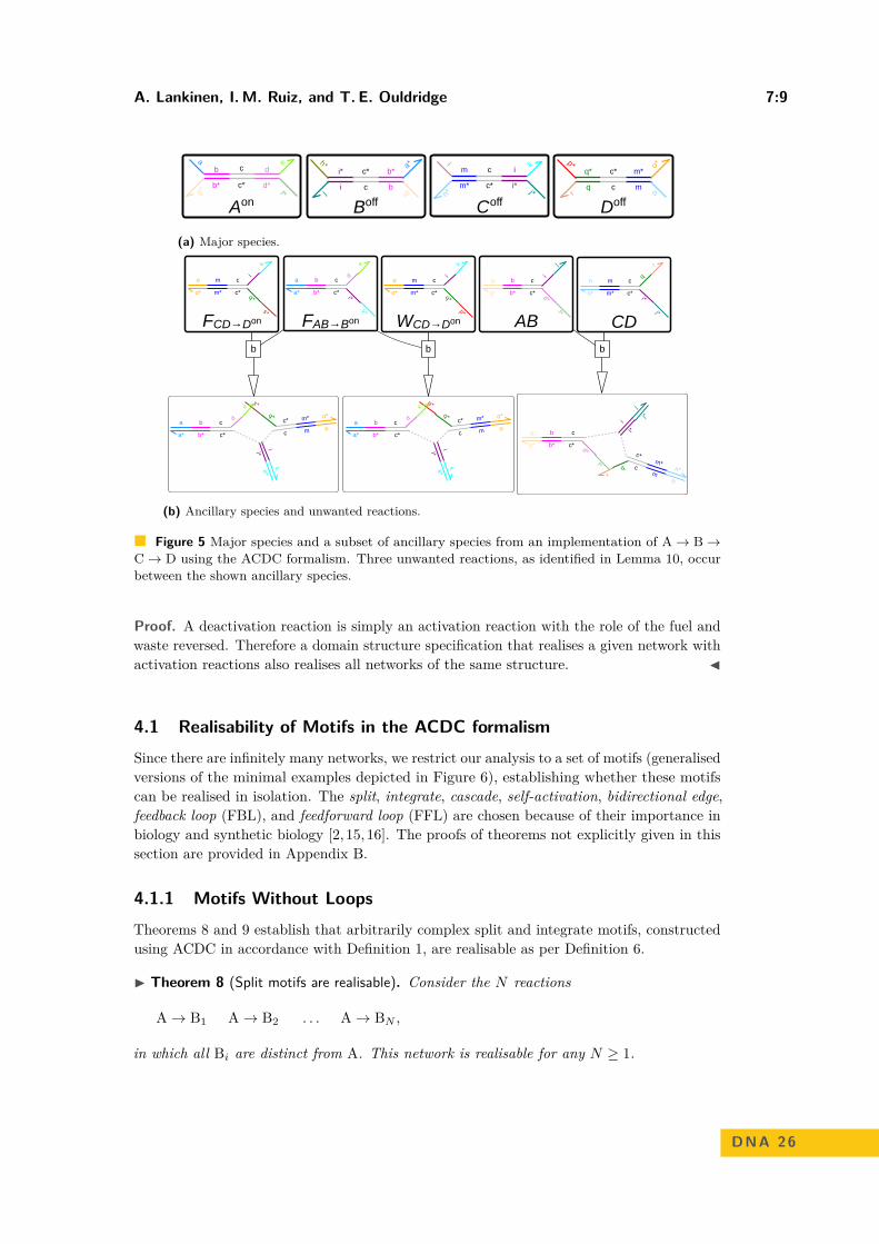
A. Lankinen, I.M. Ruiz, and T. E. Ouldridge 7:9
q* c* m*
q c m
p* o*
r n
Doff
m c i
m* c* i*
l k
n* j*
Coff
i* c* b*
i c b
h* a*
j g
Boffd*c*b*
dcb
f*g*
ea
Aon
(a) Major species.
ik
i*k*
c* m* o*
c m o
p*
q*a b c
a* b* c*
de
ik
i*k*
c* m* o*
c m o
s*
q*a b c
a* b* c*
d
e
c*m*
n*cm
nr
q
i
ji*
j*
g b c
g* b* c* d*
f*
o m c
o* m* c*
i
k
q*
p*
WCD→Don
o m c
o* m* c*
i
k
q*
s*
FCD→Don
a b c
a* b* c*
d
e
i*
k*
FAB→Bon
n m c
n* m* c*
q
r
i*
j*
CD
g b c
g* b* c*
i
j
d*
f*
AB
b b b
(b) Ancillary species and unwanted reactions.
Figure 5 Major species and a subset of ancillary species from an implementation of A → B →C → D using the ACDC formalism. Three unwanted reactions, as identified in Lemma 10, occurbetween the shown ancillary species.
Proof. A deactivation reaction is simply an activation reaction with the role of the fuel andwaste reversed. Therefore a domain structure specification that realises a given network withactivation reactions also realises all networks of the same structure. J
4.1 Realisability of Motifs in the ACDC formalismSince there are infinitely many networks, we restrict our analysis to a set of motifs (generalisedversions of the minimal examples depicted in Figure 6), establishing whether these motifscan be realised in isolation. The split, integrate, cascade, self-activation, bidirectional edge,feedback loop (FBL), and feedforward loop (FFL) are chosen because of their importance inbiology and synthetic biology [2, 15,16]. The proofs of theorems not explicitly given in thissection are provided in Appendix B.
4.1.1 Motifs Without LoopsTheorems 8 and 9 establish that arbitrarily complex split and integrate motifs, constructedusing ACDC in accordance with Definition 1, are realisable as per Definition 6.
I Theorem 8 (Split motifs are realisable). Consider the N reactions
A→ B1 A→ B2 . . . A→ BN ,
in which all Bi are distinct from A. This network is realisable for any N ≥ 1.
DNA 26
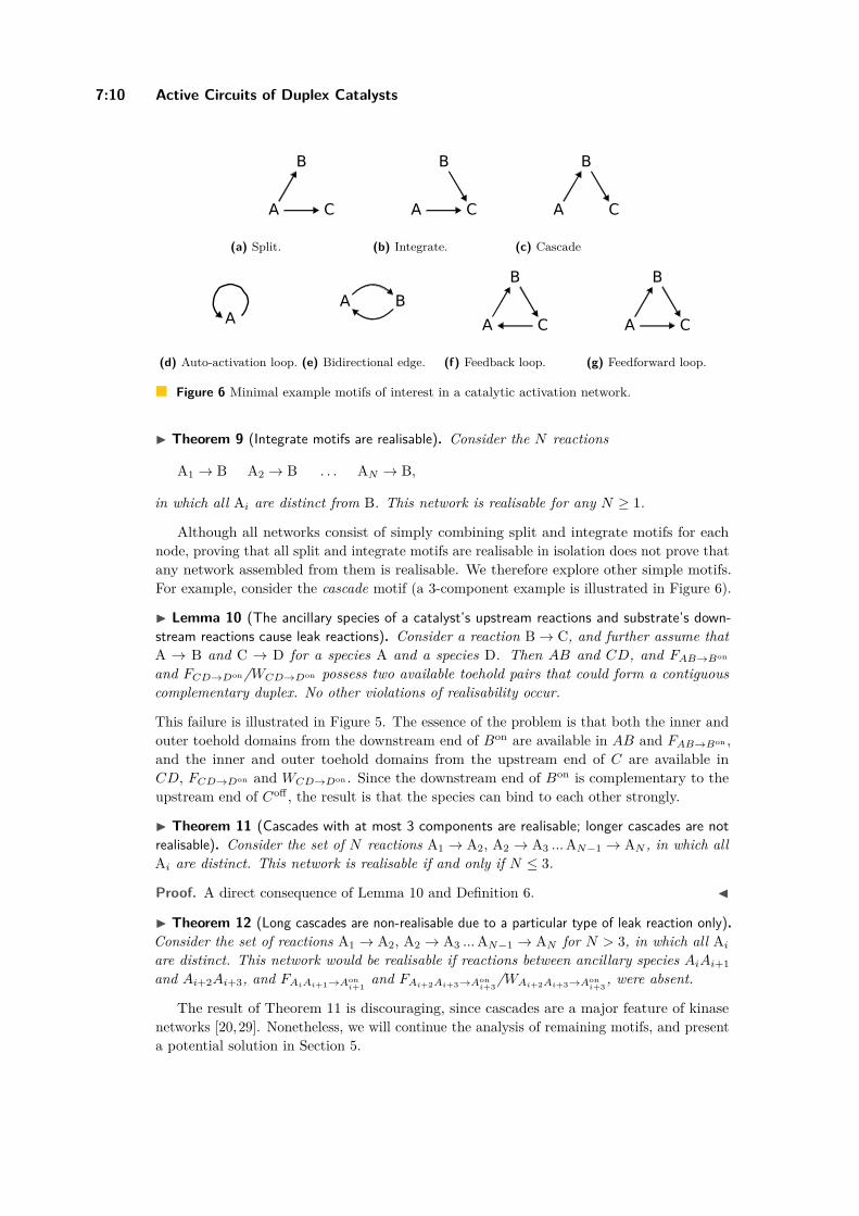
7:10 Active Circuits of Duplex Catalysts
(a) Split. (b) Integrate. (c) Cascade
(d) Auto-activation loop. (e) Bidirectional edge. (f) Feedback loop. (g) Feedforward loop.
Figure 6 Minimal example motifs of interest in a catalytic activation network.
I Theorem 9 (Integrate motifs are realisable). Consider the N reactions
A1 → B A2 → B . . . AN → B,
in which all Ai are distinct from B. This network is realisable for any N ≥ 1.
Although all networks consist of simply combining split and integrate motifs for eachnode, proving that all split and integrate motifs are realisable in isolation does not prove thatany network assembled from them is realisable. We therefore explore other simple motifs.For example, consider the cascade motif (a 3-component example is illustrated in Figure 6).
I Lemma 10 (The ancillary species of a catalyst’s upstream reactions and substrate’s down-stream reactions cause leak reactions). Consider a reaction B→ C, and further assume thatA → B and C → D for a species A and a species D. Then AB and CD, and FAB→Bon
and FCD→Don/WCD→Don possess two available toehold pairs that could form a contiguouscomplementary duplex. No other violations of realisability occur.
This failure is illustrated in Figure 5. The essence of the problem is that both the inner andouter toehold domains from the downstream end of Bon are available in AB and FAB→Bon ,and the inner and outer toehold domains from the upstream end of C are available inCD, FCD→Don and WCD→Don . Since the downstream end of Bon is complementary to theupstream end of Coff , the result is that the species can bind to each other strongly.
I Theorem 11 (Cascades with at most 3 components are realisable; longer cascades are notrealisable). Consider the set of N reactions A1 → A2, A2 → A3 ... AN−1 → AN , in which allAi are distinct. This network is realisable if and only if N ≤ 3.
Proof. A direct consequence of Lemma 10 and Definition 6. J
I Theorem 12 (Long cascades are non-realisable due to a particular type of leak reaction only).Consider the set of reactions A1 → A2, A2 → A3 ... AN−1 → AN for N > 3, in which all Ai
are distinct. This network would be realisable if reactions between ancillary species AiAi+1and Ai+2Ai+3, and FAiAi+1→Aon
i+1and FAi+2Ai+3→Aon
i+3/WAi+2Ai+3→Aon
i+3, were absent.
The result of Theorem 11 is discouraging, since cascades are a major feature of kinasenetworks [20,29]. Nonetheless, we will continue the analysis of remaining motifs, and presenta potential solution in Section 5.
A. Lankinen, I.M. Ruiz, and T. E. Ouldridge 7:11
4.1.2 Motifs With LoopsA network possesses a loop if it is possible to traverse a path that begins and ends at thesame node without using the same edge twice. For the purposes of this classification, agiven (directed) edge can be traversed in either direction. Loops are common components ofnatural networks, providing the possibility of oscillation, bistability and filtering [2, 11].
I Theorem 13 (Loops of odd length are not realisable). Consider a system of reactionsA1 ↔ A2 ↔ A3 . . . AN−1 ↔ A1, where ↔ indicates a catalytic activation in either direction.This network, a directionless loop, is not realizable if N is odd, unless the long central domainis self-complementary.
Proof. ACDC circuits require that the long central domain alternates between a sequenceand its complement in the identity strands of catalysts and their substrates. If N is odd,then the sequence must be self-complementary for this alternation to happen. J
Introducing a self-complementary central domain is a strategy that risks a competitionbetween duplexes and single-stranded hairpins. We do not consider it further.
I Theorem 14 (Self interactions and bidirectional edges are not realisable). Consider a systemof reactions A1 → A2 → A3 . . . AN−1 → A1. This network is not realisable if N ≤ 2.
The ACDC system is not inherently suited to auto-activation or bidirectional interactions.These motifs require complementarity between both the downstream and upstream toeholdsof either a single species, or two species. Strands in the system therefore violate condition 3of Definition 6 and will tend to hybridise to form fully complementary duplexes.
An isolated feedback loop is a network of size N with a single directed path around thenetwork. A simple example of length 3 is shown in Fig. 6(f).
I Theorem 15 (Feedback loops are not realisable). Consider the feedback loop A1 → A2 →A3 . . . AN−1 → A1. Such a system is not realisable for any N .
Proof. A direct consequence of Theorems 11, 13, and 14. J
As a consequence of Theorems 13 and 14, any realisable feedback loop must have N ≥ 4.However, a feedback loop of this length faces the same issues as a cascade: formation of stable,undesired products between ancillary species. As with cascades, the problem is essentiallylocal, due to interactions between ancillary species in reaction n and reaction n + 2.
I Theorem 16 (Long feedback loops with an even number of units are non-realisable due to aparticular type of leak reaction only). Consider the feedback loop
A1 → A2 A2 → A3 . . . AN−1 → AN AN → A1
For N even, N ≥ 4, this network would be realisable if reactions between ancillary speciesAiAi+1 and Ai+2Ai+3, and FAiAi+1→Aon
i+1and FAi+2Ai+3→Aon
i+3/WAi+2Ai+3→Aon
i+3, were absent.
Here, the index j in Aj should be interpreted modularly: Aj = Aj−N for j > N .
An isolated feedforward loop is a network of size N with two directed paths from onenode i to another node j. Every other node appears exactly once in one of these paths. Anexample with path lengths of 1 and 2 is shown in Figure 6.
DNA 26
7:12 Active Circuits of Duplex Catalysts
I Theorem 17 (The relative lengths of paths are constrained in feedforward loops). Considerthe generalised feedforward loop
A→ B1 B1 → B2 . . . BN−1 → BN BN → DA→ C1 C1 → C2 . . . CM−1 → CM CM → D
For such a network to be realisable, it is necessary that N ≥ 1, M ≥ 1, and N −M is even.
Proof. The claim about N −M having to be even follows from Theorem 13.Assume for contradiction that a FFL with N = 0 and M ≥ 2 and even is realisable. Since
A activates C1, and both A and CM activate D, it must be that CM can also perform a branchmigration with C1, which is an unwanted reaction violating condition 2 of Definition 6. J
Since each path in a feedforward loop is a cascade, Theorems 11 and 17 imply that onlyfeedforward loops with a single intermediate in each branch are realisable.
I Theorem 18 (Realisability of feedforward loops). Consider the generalised feedforward loop
A→ B1 B1 → B2 . . . BN−1 → BN BN → DA→ C1 C1 → C2 . . . CM−1 → CM CM → D
Such a system is realisable if and only if N = 1 and M = 1.
Proof. As a consequence of Theorems 8, 9, 11, and 17, all other FFLs are not realisable.The realisability of the FFL with N=1 and M=1 can be verified by inspection. J
Typically, feedforward loops use branches of different lengths to achieve a complexresponse to a signal over time [2,11]. Such networks are not realisable. Indeed, our analysis ofvarious motifs has revealed that the majority are not realisable. Broadly speaking, there are anumber of small motifs (e.g. auto-activation, bi-directional reactions, feedforward loops withno intermediates in one branch) that cannot be achieved because the major species themselvesinteract directly. In addition, loops of odd total length are not realisable due to the natureof complementary base pairs. However, most motifs are ruled out because of a single type ofinteraction, between the ancillary species in one reaction and the ancillary species in anotherreaction that occurs two steps downstream. In Section 5, we propose a strategy to overcomethis last problem, massively increasing the scope of the ACDC framework.
5 Overcoming the Cascade Leak Reaction and Introducing HiddenThermodynamic Drive
The most severe limitation of the ACDC system detailed in Section 3 is expressed by Theorem11. Long cascades, and loops incorporating cascades, are non-realisable due to interactionsbetween ancillary species of a given reaction, and ancillary species of a reaction separated bytwo catalytic steps (Theorem 12).
I Assumption 19 (Mismatches destabilise complexes held together by two contiguous toeholddomains). We assume that a single mismatched C-C or G-G base pair, positioned adjacent tothe interface of two toehold domains, is sufficiently destabilizing that an unwanted complexformed only by the binding of these toehold domains no longer precludes realisability.

A. Lankinen, I.M. Ruiz, and T. E. Ouldridge 7:13
The basic design of the ACDC motif assumes that toehold binding is relatively weak; twotoehold domains on either side of a junction must be able to dissociate by Assumption 2.Individual C-C or G-G mismatches are known to be highly destabilising [40], and shouldsimilarly allow for two contiguous domains to detach. Given Assumption 19, the challengeis then to systematically introduce mismatches so that all interactions between ancillaryspecies identified in Theorem 12 are compromised by a mismatch, without compromisingintended circuit activity. Our full scheme is visualised in Figure 7.
I Definition 20 (Mismatches proposed to destabilize unintended complexes). We propose thefollowing mismatches.1. We propose that the upstream interface of every major species is made distinct for active
and inactive states. Specifically, we introduce a G base at the inner edge of the outertoehold domain of the state strand of the inactive species, and a C base in the sameposition for the active species. Catalysts that (de)activate that species possess a C(G) inthe complementary position of their downstream interface.
2. We introduce a C-C mismatch at the outer edge of the inner toehold domain at thedownstream interface of each major species. This mismatch is eliminated in the formationof waste complexes, and retained in the substrate-catalyst complexes.
I Assumption 21 (Mismatches cannot cause leak reactions). We assume that the sequenceconstraints introduced by mismatch inclusion do not violate Assumption 5, and that thedestabilisation of duplexes does not violate Assumption 2.
In practice, mismatches will likely result in some increase in the rate of interactions betweenotherwise hidden toeholds; we assume that these rates remain negligible.
I Theorem 22 (Mismatches successfully destabilize unintended complexes). The schemeproposed in Definition 20 satisfies the following:1. All motifs that are realisable in the mismatch-free ACDC design remain realisable in the
mismatch-based scheme.2. Cascades of arbitrary length N with at most the first and last reactions deactivating are
realisable;3. Feedback loops with N even and N ≥ 6 in which all reactions are activating are realisable;4. Feedforward loops with N ≥ 1, M ≥ 1, N −M even, in which at most the first and last
reactions are deactivating in each branch, are realisable.
The proof of Theorem 22 is given in Appendix B.Note that the introduction of mismatches proposed in Definition 20 invalidates Lemma
7, since the downstream domains of activating and deactivating catalysts are now distinct.Indeed, the described strategy only eliminates unwanted sequestration in cascades in whichthe intermediate steps are activating. Nonetheless, it makes complex networks in which -for example - deactivating catalysts are always active realisable. Networks of this kind arecommon in biology [20,29].
The first type of mismatch in Definition 20 ensures that there is always a C-C mismatchbetween the upstream toeholds of the state strand of Aon
i+2 and the downstream toeholds ofthe state strand of Aon
i+1 in the cascade Ai → / a Ai+1 → Ai+2 → / a Ai+3, weakening theunwanted binding between the fuel and waste species identified in Theorem 12. Here → / aindicates activation or deactivation. The second type of mismatch in Definition 20 ensuresthat the upstream toeholds of the identity strand of Ai+2 are no longer fully complementaryto the downstream toeholds of Ai+1 in the cascade Ai → / a Ai+1 → / a Ai+2 → / a Ai+3,weakening the unwanted binding between ancillary species AiAi+1 and Ai+2Ai+3.
DNA 26
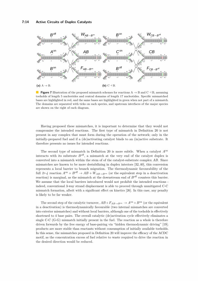
7:14 Active Circuits of Duplex Catalysts
Aone1 * d1* c* h1*
i*
jh1cd2f
NNNNCC NNNNNNNNNNNNNNNNNNNNNNNNNGNNNNNNNNNNNNNNNNNNNNNNNNNC
NNNNNC
NNNNN
NNNNN
Bonkb1 c d1
e 2
f*d1*c*b2*
g*
NNNNNC NNNNNNNNNNNNNNNNNNNNNNNNNGNNNNNNNNNNNNNNNNNNNNNNNNNC
NNNNNC
CNNNN
NNNNN
Boffab1 c d1
e 1
f*d1*c*b2*
g*
NNNNNC NNNNNNNNNNNNNNNNNNNNNNNNNGNNNNNNNNNNNNNNNNNNNNNNNNNC
NNNNNC
GNNNN
NNNNN
WAB→BonNNNNNCNNNN
NNNNNGNNNNNNNNNNNNNNNNNNNNNNNNNGGNNNNNNNNNNNNNNNNNNNNNNNNNCCNNNN
a
b1
h 1*
i*
d1
d1*
e1c
c* e1*
FAB→BonNNNNNCNNNN
NNNNNGNNNNNNNNNNNNNNNNNNNNNNNNNGCNNNNNNNNNNNNNNNNNNNNNNNNNCCNNNN
k
b1
h 1*
i*
d1
d1*
e2c
c* e1*
ABNNNNNCNNNN
NNNNNCNNNNNNNNNNNNNNNNNNNNNNNNNCNNNNNNNNNNNNNNNNNNNNNNNNNNCNNNNN
j
h1
b 2*
g*
d2
d1*
fc
c* f*
(a) A → B.
Boffab1 c d1
e 1
f*d1*c*b2*
g*
NNNNNC NNNNNNNNNNNNNNNNNNNNNNNNNGNNNNNNNNNNNNNNNNNNNNNNNNNC
NNNNNC
GNNNN
NNNNN
C one2 * d1* c* l1*
m*
nl1cd2f
NNNNGC NNNNNNNNNNNNNNNNNNNNNNNNNGNNNNNNNNNNNNNNNNNNNNNNNNNC
NNNNNC
GNNNN
NNNNN
WCB→BoffNNNNNCNNNN
NNNNNGNNNNNNNNNNNNNNNNNNNNNNNNNGGNNNNNNNNNNNNNNNNNNNNNNNNNCCNNNN
k
b1
l 1*
m*
d1
d1*
e1c
c* e1*
NNNNNCNNNN
NNNNNGNNNNNNNNNNNNNNNNNNNNNNNNNGGNNNNNNNNNNNNNNNNNNNNNNNNNCGNNNN
a
b1
l 1*
m*
d1
d1*
e1c
c* e2*
CBNNNNNCNNNN
NNNNNCNNNNNNNNNNNNNNNNNNNNNNNNNCNNNNNNNNNNNNNNNNNNNNNNNNNNCNNNNN
n
l1
b 2*
g*
d2
d1*
fc
c* f*
Bonkb1 c d1
e 2
f*d1*c*b2*
g*
NNNNNC NNNNNNNNNNNNNNNNNNNNNNNNNGNNNNNNNNNNNNNNNNNNNNNNNNNC
NNNNNC
CNNNN
NNNNN
FCB→Boff
(b) C a B.
Figure 7 Illustration of the proposed mismatch schemes for reactions A → B and C a B, assumingtoeholds of length 5 nucleotides and central domains of length 17 nucleotides. Specific mismatchedbases are highlighted in red, and the same bases are highlighted in green when not part of a mismatch.The domains are separated with ticks on each species, and upstream interfaces of the major speciesare shown on the right of each diagram.
Having proposed these mismatches, it is important to determine that they would notcompromise the intended reactions. The first type of mismatch in Definition 20 is notpresent in any complex that must form during the operation of the network; only in theinitially-prepared fuel and if a (de)activating catalyst binds to an (in)active substrate. Ittherefore presents no issues for intended reactions.
The second type of mismatch in Definition 20 is more subtle. When a catalyst Aon
interacts with its substrate Boff , a mismatch at the very end of the catalyst duplex isconverted into a mismatch within the stem of of the catalyst-substrate complex AB. Sincemismatches are known to be more destabilizing in duplex interiors [32,40], this conversionrepresents a local barrier to branch migration. The thermodynamic favourability of thefull 2r-4 reaction Aon + Boff → AB + WAB→Bon (or the equivalent step in a deactivationreaction) is marginal, as the mismatch at the downstream end of Boff counters this barrier.We assume that the local barriers introduced would not prohibit the intended reactions -indeed, conventional 3-way strand displacement is able to proceed through unmitigated C-Cmismatch formation, albeit with a significant effect on kinetics [26]. In this case, any penaltyis likely to be far weaker.
The second step of the catalytic turnover, AB +FAB→Bon → Aon +Bon (or the equivalentin a deactivation) is thermodynamically favourable (two internal mismatches are convertedinto exterior mismatches) and without local barriers, although one of the toeholds is effectivelyshortened to 4 base pairs. The overall catalytic (de)activation cycle effectively eliminates asingle C-C (G-G) mismatch initially present in the fuel. The reaction as a whole is thereforedriven forwards by the free energy of base-pairing via “hidden thermodynamic driving” [19];products are more stable than reactants without consumption of initially available toeholds.In this sense, the mismatches proposed in Definition 20 will improve the efficacy of the ACDCmotif, as the concentration excess of fuel relative to waste required to drive the reaction inthe desired direction would be reduced.

A. Lankinen, I.M. Ruiz, and T. E. Ouldridge 7:15
6 A Compiler for ACDC Networks
To construct an ACDC network that implements a given graph, three things need to be done:(1) verification that the network is realisable; (2) enumerating all domains on all speciesgiven the graph topology; and (3) compile sequences for each domain and thus for eachstrand present in the system. We have created an ACDC compiler with this functionality [24].While compilers for DSD systems that could be potentially be extended to accommodateour framework exist [3, 46], we decided to make our own since our framework has uniquerequirements about verifying the feasibility of a given CRN and introducing mismatcheswithin domains.
The first part is done, at least at the level of each cascade and loop present, by analysingthe properties of a given graph. For every pair of nodes i, j, all directed simple paths arecomputed. We search for paths of length N ≥ 3 that containing edge weights of -1 anywhereother than at the first or last edge; these cascades are not rendered realisable by our mismatchscheme, per Theorem 22. Moreover, if there exists more than 1 path between the nodes,then either a FFL (at least two paths from i to j or from j to i) or a FBL (at least one pathfrom i to j and from j to i) exists in the graph. Furthermore, if there exists more than 1path between the nodes after transforming the graph to an undirected form, there existsa “directionless loop” (Theorem 13) in the graph. The realisability of the loop(s) can beverified from the lengths of the paths according to Theorems 13 and 22.
If a given graph is found to be realisable, then domains are assigned for each strand ofeach species, such that all complementarities and mismatches required by the topology aresatisfied. This ask can be achieved by local analysis of the network topology.
Finally, a NUPACK [54] script is generated to generate optimal sequences for each strand.The required mismatches are hard-coded into the domain definitions in the script. Thesoftware is available at https://zenodo.org/record/3948343.
7 Discussion
We have introduced the ACDC scheme for constructing DNA-based networks that performdirect catalysis, analysed its shortcomings, and subsequently proposed practical improvements.As of now, we have focused only on the realisability of ACDC implementations for somegraphs, not their dynamical behaviour. Three natural directions for further theoreticalinvestigation are: (1) proving the realisability of arbitrary networks; (2) implementingadditional hidden thermodynamic driving so that both 2r-4 substeps of a catalytic reactionare thermodynamically downhill; and (3) automated design of ACDC networks to performsome desired transfer function between input concentrations xi(t), i = 1..N and outputconcentrations yj(t), j = 1..M . With regard to the first, we conjecture that all violations ofrealisability in arbitrary networks are attributable to the causes identified in Section 4.
Equally important, however, is experimentally testing the ACDC motif. Whilst 4-waybranch migration has been used in several contexts [10, 22, 25, 49], the toehold exchangemechanism proposed here is relatively untested. It is also important to establish that themismatches function as intended, limiting sequestration reactions and providing strongoverall thermodynamic driving without causing excessive local barriers that frustrate thenecessary reactions. A final consideration is the possibility of leak reactions involving non-complementary toeholds that we have assumed to be negligible. It remains to be establishedthat unintended reactions will occur at a negligible rate, particularly in the context of speciescontaining mismatches. This research is ongoing within the group.
DNA 26

7:16 Active Circuits of Duplex Catalysts
A key property of ACDC is the two recognition interfaces within each species and theinherent symmetry in the species that follows. While this symmetry is a design featurethat allows both substrate-like and catalyst-like behaviour for a single species, it also hasa drawback that domains that are essential for some reaction to occur are also present inreactions where they only act as identity placeholders (downstream interface of a catalyst andan upstream interface of a substrate) that do not interact with any other domain. Considerthe reaction in Figure 4; the identity of the “placeholder domains” a, b, g, h, i, j, k that aren’tinvolved in the initial binding and migration reactions could be swapped to arbitrary domainsthat aren’t complementary with d, e, f or each other in only one species and the reactioncould still occur (assuming the correct fuel species is generated based on the substrate andcatalyst). However, this may not be possible if A and B are part of some larger computationalnetwork where the placeholder domain identities are important. Another drawback of thesymmetry is the limitation of loop lengths to even numbers, characterised in Theorem 13.An obvious potential mitigation to this problem is to make the central domain its owncomplement, although this choice risks the formation of self-complementary hairpins.
The weaknesses of the ACDC motif invite the exploration of other possible designs ofcatalytic activation networks that operate via direct bimolecular catalysis. It is an openquestion as to whether the shortcomings of ACDC can be mitigated without a substantialincrease in complexity or abandoning the mechanism of direct catalytic action.
8 Conclusion
We have established the concept of a direct catalytic reaction and discussed why previouswork on catalytic DNA computing does not fulfil this definition. We have then proposeda framework, ACDC, for implementing non-equilibrium catalytic (de)activation networksusing direct catalytic activation, analogous to systems seen in living cells. ACDC is simplein the sense that all species contain only two strands - an important consideration in thecontext of implementing DSD circuitry in a broad range of contexts.
We have analysed the framework’s expressiveness by exploring the implementation ofseven network motifs with ACDC. The basic design is highly limited by the inherent symmetryof components, prohibiting long cascades and most feedforward and feedback loops. However,we propose that systematic placement of mismatches can obviate these difficulties in manycontexts. Moreover, we argue that these initially-present mismatches can contribute a “hiddenthermodynamic driving” [19] to the ACDC motifs, increasing the robustness of the designto subtleties in DNA thermodynamics and reducing the concentration imbalances of fuelsrequired to drive the reactions forward. We present a compiler for the sequence design ofACDC-based networks that implements these findings [24].
References1 Leonard Adleman. Molecular computation of solutions to combinatorial problems. Science,
266(5187):1021–1024, November 1994. doi:10.1126/science.7973651.2 Uri Alon. An introduction to systems biology: design principles of biological circuits, Second
Edition. CRC Press LLC, Boca Raton, UNITED STATES, 2019.3 Stefan Badelt, Seung Woo Shin, Robert F. Johnson, Qing Dong, Chris Thachuk, and
Erik Winfree. A general-purpose CRN-to-DSD compiler with formal verification, optim-ization, and simulation capabilities. In DNA computing and molecular programming, Lec-ture notes in computer science, pages 232–248. Springer, Cham, September 2017. doi:10.1007/978-3-319-66799-7_15.

A. Lankinen, I.M. Ruiz, and T. E. Ouldridge 7:17
4 David Barford, Amit K. Das, and Marie-Pierre Egloff. The structure and mechanism ofprotein phosphatases: insights into catalysis and regulation. Annual Review of Biophysicsand Biomolecular Structure, 27(1):133–164, June 1998. Publisher: Annual Reviews. doi:10.1146/annurev.biophys.27.1.133.
5 John P. Barton and Eduardo D. Sontag. The energy costs of insulators in biochemical networks.Biophysical Journal, 104(6):1380–1390, March 2013. doi:10.1016/j.bpj.2013.01.056.
6 Hieu Bui, Shalin Shah, Reem Mokhtar, Tianqi Song, Sudhanshu Garg, and John Reif. LocalizedDNA hybridization chain reactions on DNA origami. ACS Nano, 12(2):1146–1155, February2018. Publisher: American Chemical Society. doi:10.1021/acsnano.7b06699.
7 Gourab Chatterjee, Neil Dalchau, Richard A. Muscat, Andrew Phillips, and Georg Seelig. Aspatially localized architecture for fast and modular DNA computing. Nature Nanotechnology,12(9):920–927, September 2017. Number: 9 Publisher: Nature Publishing Group. doi:10.1038/nnano.2017.127.
8 Yuan-Jyue Chen, Neil Dalchau, Niranjan Srinivas, Andrew Phillips, Luca Cardelli, DavidSoloveichik, and Georg Seelig. Programmable chemical controllers made from DNA. NatureNanotechnology, 8(10):755–762, October 2013. doi:10.1038/nnano.2013.189.
9 Kevin M. Cherry and Lulu Qian. Scaling up molecular pattern recognition with DNA-based winner-take-all neural networks. Nature, 559(7714):370–376, July 2018. doi:10.1038/s41586-018-0289-6.
10 Nadine L. Dabby. Synthetic molecular machines for active self-assembly: prototype al-gorithms, designs, and experimental study. PhD thesis, California Institute of Tech-nology, Pasadena, California, 2013. URL: https://pdfs.semanticscholar.org/e668/440cdb786ea7c2d0d6ae306c5aefef1208f6.pdf.
11 Wiet de Ronde and Pieter Rein ten Wolde. Multiplexing oscillatory biochemical signals.Physical Biology, 11(2):026004, April 2014. doi:10.1088/1478-3975/11/2/026004.
12 Abhishek Deshpande and Thomas E. Ouldridge. High rates of fuel consumption are not requiredby insulating motifs to suppress retroactivity in biochemical circuits. Engineering Biology,1(2):86–99, December 2017. Publisher: IET Digital Library. doi:10.1049/enb.2017.0017.
13 Robert M. Dirks, Justin S. Bois, Joseph M. Schaeffer, Erik Winfree, and Niles A. Pierce.Thermodynamic analysis of interacting nucleic acid strands. SIAM Review, 49(1):65–88,January 2007. Publisher: Society for Industrial and Applied Mathematics. doi:10.1137/060651100.
14 Elaine A. Elion. Ste5: a meeting place for MAP kinases and their associates. Trends in CellBiology, 5(8):322–327, August 1995. doi:10.1016/S0962-8924(00)89055-8.
15 Michael B. Elowitz and Stanislas Leibler. A synthetic oscillatory network of transcriptionalregulators. Nature, 403(6767):335–338, January 2000. Number: 6767 Publisher: NaturePublishing Group. doi:10.1038/35002125.
16 Timothy S. Gardner, Charles R. Cantor, and James J. Collins. Construction of a genetictoggle switch in Escherichia coli. Nature, 403(6767):339–342, January 2000. Number: 6767Publisher: Nature Publishing Group. doi:10.1038/35002131.
17 Anthony J. Genot, Teruo Fujii, and Yannick Rondelez. Scaling down DNA circuits withcompetitive neural networks. Journal of The Royal Society Interface, 10(85):20130212, August2013. Publisher: Royal Society. doi:10.1098/rsif.2013.0212.
18 Christopher C. Govern and Pieter Rein ten Wolde. Energy dissipation and noise correlationsin biochemical sensing. Physical Review Letters, 113(25):258102, December 2014. Publisher:American Physical Society. doi:10.1103/PhysRevLett.113.258102.
19 Natalie E. C. Haley, Thomas E. Ouldridge, Ismael Mullor Ruiz, Alessandro Geraldini, Ard A.Louis, Jonathan Bath, and Andrew J. Turberfield. Design of hidden thermodynamic driving fornon-equilibrium systems via mismatch elimination during DNA strand displacement. NatureCommunications, 11(1):2562, May 2020. Number: 1 Publisher: Nature Publishing Group.doi:10.1038/s41467-020-16353-y.
DNA 26

7:18 Active Circuits of Duplex Catalysts
20 Ira Herskowitz. MAP kinase pathways in yeast: for mating and more. Cell, 80(2):187–197,January 1995. doi:10.1016/0092-8674(95)90402-6.
21 Robert F. Johnson. Impossibility of sufficiently simple chemical reaction network imple-mentations in DNA strand displacement. In Ian McQuillan and Shinnosuke Seki, editors,Unconventional computation and natural computation, Lecture notes in computer science, pages136–149. Springer International Publishing, 2019. doi:10.1007/978-3-030-19311-9_12.
22 Shohei Kotani and William L. Hughes. Multi-arm junctions for dynamic DNA nanotechnology.Journal of the American Chemical Society, 139(18):6363–6368, May 2017. doi:10.1021/jacs.7b00530.
23 Matthew R. Lakin, Simon Youssef, Filippo Polo, Stephen Emmott, and Andrew Phillips.Visual DSD: a design and analysis tool for DNA strand displacement systems. Bioinformatics,27(22):3211–3213, November 2011. doi:10.1093/bioinformatics/btr543.
24 Antti Lankinen. ACDC compiler, July 2020. URL: https://zenodo.org/record/3948343.25 Tong Lin, Jun Yan, Luvena L. Ong, Joanna Robaszewski, Hoang D. Lu, Yongli Mi, Peng Yin,
and Bryan Wei. Hierarchical assembly of DNA nanostructures based on four-way toehold-mediated strand displacement. Nano Letters, 18(8):4791–4795, August 2018. Publisher:American Chemical Society. doi:10.1021/acs.nanolett.8b01355.
26 Robert R. F. Machinek, Thomas E. Ouldridge, Natalie E. C. Haley, Jonathan Bath, andAndrew J. Turberfield. Programmable energy landscapes for kinetic control of DNA stranddisplacement. Nature Communications, 5(1):1–9, November 2014. Number: 1 Publisher:Nature Publishing Group. doi:10.1038/ncomms6324.
27 Marcelo O. Magnasco. Chemical kinetics is Turing universal. Physical Review Letters,78(6):1190–1193, February 1997. doi:10.1103/PhysRevLett.78.1190.
28 G. Manning, D. B. Whyte, R. Martinez, T. Hunter, and S. Sudarsanam. The proteinkinase complement of the human genome. Science, 298(5600):1912–1934, December 2002.Publisher: American Association for the Advancement of Science Section: Review. doi:10.1126/science.1075762.
29 Christopher J. Marshall. MAP kinase kinase kinase, MAP kinase kinase and MAP kinase.Current Opinion in Genetics & Development, 4(1):82–89, February 1994. doi:10.1016/0959-437X(94)90095-7.
30 Pankaj Mehta, Alex H. Lang, and David J. Schwab. Landauer in the agea of synthetic biology:energy consumption and information processing in biochemical networks. Journal of StatisticalPhysics, 162(5):1153–1166, March 2016. doi:10.1007/s10955-015-1431-6.
31 Thomas E. Ouldridge, Christopher C. Govern, and Pieter Rein ten Wolde. Thermodynamicsof computational copying in biochemical systems. Physical Review X, 7(2):021004, April 2017.Publisher: American Physical Society. doi:10.1103/PhysRevX.7.021004.
32 Thomas E. Ouldridge, Ard A. Louis, and Jonathan P. K. Doye. Structural, mechanical,and thermodynamic properties of a coarse-grained DNA model. The Journal of ChemicalPhysics, 134(8):085101, February 2011. Publisher: American Institute of Physics. doi:10.1063/1.3552946.
33 Tomislav Plesa. Stochastic approximation of high-molecular by bi-molecular reactions.arXiv:1811.02766 [math, q-bio], November 2018. arXiv: 1811.02766. URL: http://arxiv.org/abs/1811.02766.
34 Lulu Qian, David Soloveichik, and Erik Winfree. Efficient Turing-universal computationwith DNA polymers. In Yasubumi Sakakibara and Yongli Mi, editors, DNA computing andmolecular programming, Lecture notes in computer science, pages 123–140, Berlin, Heidelberg,2011. Springer. doi:10.1007/978-3-642-18305-8_12.
35 Lulu Qian and Erik Winfree. Scaling up digital circuit computation with DNA stranddisplacement cascades. Science, 332(6034):1196–1201, June 2011. doi:10.1126/science.1200520.

A. Lankinen, I.M. Ruiz, and T. E. Ouldridge 7:19
36 Lulu Qian and Erik Winfree. A simple DNA gate motif for synthesizing large-scale circuits.Journal of the Royal Society Interface, 8(62):1281–1297, September 2011. doi:10.1098/rsif.2010.0729.
37 Lulu Qian and Erik Winfree. Parallel and scalable computation and spatial dynamics withDNA-based chemical reaction networks on a surface. In Satoshi Murata and Satoshi Kobayashi,editors, DNA computing and molecular programming, Lecture notes in computer science, pages114–131, Cham, 2014. Springer International Publishing. doi:10.1007/978-3-319-11295-4_8.
38 Lulu Qian, Erik Winfree, and Jehoshua Bruck. Neural network computation with DNA stranddisplacement cascades. Nature, 475(7356):368–372, July 2011. doi:10.1038/nature10262.
39 Ismael Mullor Ruiz, Jean-Michel Arbona, Amitkumar Lad, Oscar Mendoza, Jean-Pierre Aimé,and Juan Elezgaray. Connecting localized DNA strand displacement reactions. Nanoscale,7(30):12970–12978, July 2015. Publisher: The Royal Society of Chemistry. doi:10.1039/C5NR02434J.
40 John SantaLucia and Donald Hicks. The thermodynamics of DNA structural motifs. An-nual Review of Biophysics and Biomolecular Structure, 33(1):415–440, 2004. _eprint: ht-tps://doi.org/10.1146/annurev.biophys.32.110601.141800. doi:10.1146/annurev.biophys.32.110601.141800.
41 Hans J. Schaeffer, Andrew D. Catling, Scott T. Eblen, Lara S. Collier, Anke Krauss, andMichael J. Weber. MP1: a MEK binding partner that enhances enzymatic activation of theMAP kinase cascade. Science, 281(5383):1668–1671, September 1998. Publisher: AmericanAssociation for the Advancement of Science Section: Report. doi:10.1126/science.281.5383.1668.
42 Georg Seelig, David Soloveichik, David Yu Zhang, and Erik Winfree. Enzyme-free nucleic acidlogic circuits. Science, 314(5805):1585–1588, December 2006. Publisher: American Associationfor the Advancement of Science Section: Report. doi:10.1126/science.1132493.
43 Nadrian C. Seeman and Hanadi F. Sleiman. DNA nanotechnology. Nature Reviews Materials,3(1):1–23, November 2017. doi:10.1038/natrevmats.2017.68.
44 David Soloveichik, Georg Seelig, and Erik Winfree. DNA as a universal substrate for chemicalkinetics. Proceedings of the National Academy of Sciences, 107(12):5393–5398, March 2010.doi:10.1073/pnas.0909380107.
45 Carlo Spaccasassi, Matthew R. Lakin, and Andrew Phillips. A logic programming languagefor computational nucleic acid devices. ACS synthetic biology, 8(7):1530–1547, July 2019.doi:10.1021/acssynbio.8b00229.
46 Niranjan Srinivas, James Parkin, Georg Seelig, Erik Winfree, and David Soloveichik. Enzyme-free nucleic acid dynamical systems. Science, 358(6369), December 2017. doi:10.1126/science.aal2052.
47 J. David Sweatt. The neuronal MAP kinase cascade: a biochemical signal integration systemsubserving synaptic plasticity and memory. Journal of Neurochemistry, 76(1):1–10, 2001.doi:10.1046/j.1471-4159.2001.00054.x.
48 Mario Teichmann, Enzo Kopperger, and Friedrich C. Simmel. Robustness of localized DNAstrand displacement cascades. ACS Nano, 8(8):8487–8496, August 2014. Publisher: AmericanChemical Society. doi:10.1021/nn503073p.
49 Suvir Venkataraman, Robert M. Dirks, Paul W. K. Rothemund, Erik Winfree, and Niles A.Pierce. An autonomous polymerization motor powered by DNA hybridization. NatureNanotechnology, 2(8):490–494, August 2007. Number: 8 Publisher: Nature Publishing Group.doi:10.1038/nnano.2007.225.
50 Alan J. Whitmarsh, Julie Cavanagh, Cathy Tournier, Jun Yasuda, and Roger J. Davis.A mammalian scaffold complex that selectively mediates MAP kinase activation. Science,281(5383):1671–1674, September 1998. Publisher: American Association for the Advancementof Science Section: Report. doi:10.1126/science.281.5383.1671.
51 Christian Widmann, Spencer Gibson, Matthew B. Jarpe, and Gary L. Johnson. Mitogen-activated protein kinase: conservation of a three-kinase module from yeast to human. Physiolo-
DNA 26

7:20 Active Circuits of Duplex Catalysts
gical Reviews, 79(1):143–180, January 1999. Publisher: American Physiological Society.doi:10.1152/physrev.1999.79.1.143.
52 Wataru Yahiro and Masami Hagiya. Implementation of Turing machine using DNA stranddisplacement. In Carlos Martín-Vide, Takaaki Mizuki, and Miguel A. Vega-Rodríguez, editors,Theory and Practice of Natural Computing, Lecture notes in computer science, pages 161–172,Cham, 2016. Springer International Publishing. doi:10.1007/978-3-319-49001-4_13.
53 Peng Yin, Harry M. T. Choi, Colby R. Calvert, and Niles A. Pierce. Programming biomolecularself-assembly pathways. Nature, 451(7176):318–322, January 2008. Number: 7176 Publisher:Nature Publishing Group. doi:10.1038/nature06451.
54 Joseph N. Zadeh, Conrad D. Steenberg, Justin S. Bois, Brian R. Wolfe, Marshall B. Pierce,Asif R. Khan, Robert M. Dirks, and Niles A. Pierce. NUPACK: Analysis and design of nucleicacid systems. Journal of Computational Chemistry, 32(1):170–173, 2011. doi:10.1002/jcc.21596.
55 David Yu Zhang and Georg Seelig. Dynamic DNA nanotechnology using strand-displacementreactions. Nature Chemistry, 3(2):103–113, February 2011. doi:10.1038/nchem.957.
56 David Yu Zhang, Andrew J. Turberfield, Bernard Yurke, and Erik Winfree. Engineeringentropy-driven reactions and networks catalyzed by DNA. Science, 318(5853):1121–1125,November 2007. Publisher: American Association for the Advancement of Science Section:Report. doi:10.1126/science.1148532.
A Notation For ACDC Species and Reactions
[a b] denotes a strand consisting of domains a and b. Logical not is denoted by ¬ and logicaland by ∧.
I Definition 23. (ACDC major species structure). Each major species in an ACDC networkconsists of two strands, each of which have one long domain and four toehold domains. Thetwo strands are called state strand and identity strand based on the fact that one stranddecodes the state of the species and other the identity. A major species X has the followingdomains (note the use of H for “inner” to avoid confusion with “identity”):
SH5(X): the inner toehold domain on the 5’ side (downstream end) of the state strand.SO5(X): the outer toehold domain on the 5’ side (downstream end) of the state strand.SH3(X): the inner toehold domain on the 3’ side (upstream end) of the state strand.SO3(X): the outer toehold domain on the 3’ side (upstream end) of the state strand.IH5(X): the inner toehold domain on the 5’ side (upstream end) of the identity strand.IO5(X): the outer toehold domain on the 5’ side (upstream end) of the identity strand.IH3(X): the inner toehold domain on the 3’ side (downstream end) of the identity strand.IO3(X): the outer toehold domain on the 3’ side (downstream end) of the identity strand.SL(X): the long domain on the state strand.IL(X): the long domain on the identity strand.
I Definition 24. (Subset and logical operations for ACDC species). The following operationswill be useful in the analysis of ACDC networks:
Complementarity : x y is true for sequences x, y iff x = y∗ (and x∗ = y).Complementarity with mismatch : xy is true for sequences x, y iff x = y∗ (andx∗ = y) except for a single centrally-placed C-C or G-G mismatch. xy is distinct from¬x y, for which it is assumed that interactions between x and y are negligible.5′ (downstream end) state toehold sequence S5(X) := [SO5(X) SH5(X)].3′ (upstream end) state toehold sequence S3(X) := [SH3(X) SO3(X)].5′ (upstream end) identity toehold sequence I5(X) := [IO5(X) IH5(X)].3′ (downstream end) identity toehold sequence I3(X) := [IH3(X) IO3(X)].

A. Lankinen, I.M. Ruiz, and T. E. Ouldridge 7:21
I Definition 25. (Major species). A major species X must satisfy
¬(SO5(X) IO3(X)
)∧(SH5(X) IH3(X)
)∧(
SL(X) IL(X))∧(
SH3(X) IH5(X))∧ ¬(SO3(X) IO5(X)
).
I Definition 26. (Domain complementarities in an ACDC reaction without mismatches).An ACDC reaction A→ B or A a B implies
S5(Aon) S3(Boff) = S3(Bon) ∧IL(Aon) = IL(Aoff) IL(Boff) = IL(Bon) ∧I3(Aon) = I3(Aoff) I5(Boff) = I5(Bon).
Domains not constrained by these requirements are non-complementary. We emphasize thatthe domains of ancillary species involved in A → B are determined unambiguously by thedomains of the relevant major species.
I Definition 27. (Domain complementarities in ACDC reactions with mismatches). AnACDC reaction A→ / a B with mismatches placed as per Definition 20 implies
S5(Aon) S3(Boff) / S5(Aon)S3(Boff) ∧S5(Aon)S3(Bon) / S5(Aon) S3(Bon) ∧IL(Aon) = IL(Aoff) IL(Boff) = IL(Bon) ∧I3(Aon) = I3(Aoff)I5(Boff) = I5(Bon).
Domains not constrained by these requirements are non-complementary.
B Proofs of Theorems and Lemmas 8 - 22
I Theorem 8 (Split motifs are realisable). Consider the N reactions A→ B1, A→ B2, . . . A→BN , in which all Bi are distinct from A. Such a network is realisable for any N ≥ 1.
Proof. By induction. Assume that the split motif is realisable for a given N = M >
0. If so, a valid domain level implementation exists for N = M . Now consider thespecies Boff
M+1, BonM+1, ABM+1WABM+1→Bon
M+1, FABM+1→Bon
M+1related to a putative additional
node BM+1. Let these species be identical to those of B1, except with the domains thatfunction as the downstream end (SO5, SH5, IO3, IH3) in Boff
M+1, BonM+1 changed to have no
complementarity with any domains in the existing valid implementation for N = M . Thisassignment is possible by Assumption 5. Since the upstream domains SO3, SH3, IO5, IH5 ofBon
M+1, BoffM+1 are identical to those of Bon
1 , Boff1 , Definition 26 implies A→ B as required by
condition 1 of Definition 6. Moreover, since the species related to node BM+1 are identical tothose of the existing node B1, except for the downstream domains with no complementarityto the rest of the network, no new violations of conditions 2-4 of Definition 6 can occurdue to interactions between the species related to BM+1 and Aon or those related to Bi for1 < i ≤ M . By considering the species defined in Figure 4 for B1, and replacing domainsh, i, j, k with hM+1, iM+1, jM+1, kM+1 to define BM+1, it is straightforward to establish thatno violations of conditions 2-4 of Definition 6 occur between the species related to BM+1 andB1. Therefore if a split motif of size N = M is realisable, a split motif of size N = M + 1 isrealisable. Given the valid implementation for N = 1 in Figure 4, split motifs of arbitraryN > 0 are realisable. J
DNA 26

7:22 Active Circuits of Duplex Catalysts
I Theorem 9 (Integrate motifs are realisable). Consider the N reactions A1 → B, A2 →B, . . . AN → B, in which all Ai are distinct from B. This network is realisable for any N ≥ 1.
Proof. The proof is identical to that of Theorem 8 with the direction of catalysis interchanged.J
I Lemma 10 (The ancillary species of a catalyst’s upstream reactions and substrate’s down-stream reactions cause leak reactions). Consider a reaction B→ C, and further assume thatA → B and C → D for a species A and a species D. Then AB and CD, and FAB→Bon
and FCD→Don/WCD→Don possess two available toehold pairs that could form a contiguouscomplementary duplex. No other violations of realisability occur.
Proof. Consider the following major species:
Aon := [a b c d e ][g∗ b∗ c∗ d∗ f∗]
Boff := [h∗ i∗ c∗ b∗ a∗] Bon := [k∗ i∗ c∗ b∗ a∗][j i c b g ] [j i c b g ]
Coff := [l m c i k ] Con := [o m c i k ][n∗ m∗ c∗ i∗ j∗] [n∗ m∗ c∗ i∗ j∗]
Doff := [p∗ q∗ c∗ m∗ o∗] Don := [s∗ q∗ c∗ m∗ o∗][r q c m n ] [r q c m n ]
where the top (bottom) strand of each species is the state (identity) strand in 5’-3’ (3’-5’)direction. These species and the accordingly generated ancillary species implement thecascade A→ B→ C→ D. Conditions 1-3 of Definition 6 are satisfied.
To establish whether condition 4 of Definition 6 is necessarily violated, consider theunbound domains on the ancillary species in the system A→ B→ C→ D:
I5(Aoff), I3(Boff) in AB
S3(Aon), S5(Bon) in FAB→Bon
S3(Aon), S5(Boff) in WAB→Bon
I5(Boff), I3(Coff) in BC
S3(Bon), S5(Con) in FBC→Con
S3(Bon), S5(Coff) in WBC→Con
I5(Coff), I3(Doff) in CD
S3(Con), S5(Don) in FCD→Don
S3(Con), S5(Doff) in WCD→Don .Definition 26 requires that I3(Boff) I5(Coff), S5(Bon) S3(Con). These constraints aremanifested in the example above as [j, i] being present in the identity strand of Boff/Bon
and [i∗, j∗] in the identity strand of Coff/Con, and [i, k] being present in the state strandof Coff/Con and [k∗, i∗] in the state strand of Bon. Consequently AB and BC can bindby the two contiguous toehold domains I3(Boff), I5(Coff), and FAB→Bon can bind withFCD→Don and WCD→Don by the two contiguous toehold domains in S5(Bon), S3(Con). Noother violations of condition 4 occur in the proposed implementation. J
I Theorem 12 (Long cascades are non-realisable due to a particular type of leak reaction only).Consider the set of reactions A1 → A2, A2 → A3 ... AN−1 → AN for N > 3, in which all Ai
are distinct. This network would be realisable if reactions between ancillary species AiAi+1and Ai+2Ai+3, and FAiAi+1→Aon
i+1and FAi+2Ai+3→Aon
i+3/WAi+2Ai+3→Aon
i+3, were absent.

A. Lankinen, I.M. Ruiz, and T. E. Ouldridge 7:23
Proof. By induction. Assume that an implementation of a cascade of length N > 3 exists inwhich: (a) for any toehold domain x present in the downstream [upstream] end of Aoff
M orAon
M , S5(AoffM ), S5(Aon
M ), I3(AoffM ) = I3(Aon
M )[S3(Aoff
M ) = S3(AonM ), I5(Aoff
M ) = I5(AonM )], the
presence of x and x∗ in major species is restricted to the downstream [upstream] end of AoffM and
AonM and the upstream [downstream] end of Aoff
M+1 and AonM+1 [Aoff
M−1 and AonM−1], S3(Aoff
M+1) =S3(Aon
M+1), I5(AoffM+1) = I5(Aon
M+1)[S5(Aoff
M−1), S5(AonM−1), I3(Aoff
M−1) = I3(AonM−1)
]; and
(b) the only violations of realisability are those stated in this theorem. Lemma 10 gives animplementation for N = 4 satisfying these conditions.
Let us consider adding a new layer AN+1 to the cascade. The toeholds S3(AoffN+1) =
S3(AonN+1), I5(Aoff
N+1) = I5(AonN+1) are complements of S5(Aon
N ), I3(AonN ), respectively, and
the toeholds S5(AoffN+1), S5(Aon
N+1), I3(AoffN+1) = I3(Aon
N+1) can be orthogonal to all othertoeholds by Assumption 5. This choice preserves assumption (a) above for the N + 1-layer cascade. Definition 26 indicates that when the implied ancillary species are included,AN → AN+1 as required by condition 1 of Definition 6. Moreover, the only toeholds in thenew species are either non-complementary to the rest of the network, or taken from theupstream and downstream ends of Aoff
N and AonN . By (a), these toeholds are only present in
major species of nodes AN−1, AN and AN+1 and the ancillary species associated with them.To identify violations of conditions 2-4 of Definition 6, it is therefore sufficient to considerthe isolated 4-level cascade AN−2 → AN−1 → AN → AN+1 only. This analysis proceedsexactly as in Lemma 10; the proposed N + 1-layer cascade therefore preserves assumption(b) as well as (a). Given that a domain-level implementation satisfying assumption (a) and(b) is given in Lemma 10 for N = 4, we therefore conclude that an implementation satisfying(a) and (b) can be constructed for arbitrary N > 3. Consequently there are no restrictionson realisability of cascades for N > 3 other than those stated in the theorem. J
I Theorem 14 (Self interactions and bidirectional edges are not realisable). Consider a systemof reactions A1 → A2 → A3 . . . AN−1 → A1. This network is not realisable if N ≤ 2.
Proof. The result for N = 1 is a direct consequence of Theorem 13. For N = 2, consider theset of reactions: A→ B, B→ A. By Definition 26, A→ B implies I3(Aoff) I5(Boff) andIL(Aoff) IL(Boff). In addition, B→ A implies I5(Aoff) I3(Boff). The identity strands ofA and B are then fully complementary, violating condition 3 of Definition 6. J
I Theorem 16 (Long feedback loops with an even number of units are non-realisable due to a par-ticular type of leak reaction only). Consider the feedback loop A1 → A2, A2 → A3, . . . AN−1 →AN , AN → A1. For N even, N ≥ 4, this network would be realisable if reactions between ancil-lary species AiAi+1 and Ai+2Ai+3, and FAiAi+1→Aon
i+1and FAi+2Ai+3→Aon
i+3/WAi+2Ai+3→Aon
i+3,
were absent. Here, the index j in Aj should be interpreted modularly: Aj = Aj−N for j > N .
Proof. For N even, N ≥ 4, a loop obeying condition 1 of Definition 6 can be constructed fromthe cascades identified in the proof of Theorem 12 by setting the otherwise unconstrainedtoeholds S5(Aon
N ), I3(AonN ) to S5(Aon
N ) S3(Aoff1 ) = S3(Aon
1 ), I3(AonN ) I5(Aoff
1 ) = I5(Aoff1 ).
To identify the violations of realisability that arise from conditions 2-4 of Definition 6, let usfirst consider a cascade without the AN → A1 reaction. The only violations of realisabilityare those identified in Theorem 12: between AiAi+1 and Ai+2Ai+3, and FAiAi+1→Aon
i+1
and FAi+2Ai+3→Aoni+3
/WAi+2Ai+3→Aoni+3
, without interpreting the index modularly. Now weconsider the additional effect of requiring AN → A1. The only domains that must bechanged are S5(Aon
N ) and I3(AonN ). These domains and their complements are only present
in the species of AN−1 → AN , AN → A1, A1 → A2, and so it is sufficient to consider onlythis cascade to identify additional violations of realisability. By Lemma 10, the resultantviolations of realisability are exactly those stated in the theorem. J
DNA 26

7:24 Active Circuits of Duplex Catalysts
I Theorem 22 (Mismatches successfully destabilize unintended complexes). The schemeproposed in Definition 20 satisfies the following:1. All motifs that are realisable in the mismatch-free ACDC design remain realisable in the
mismatch-based scheme.2. Cascades of arbitrary length N with at most the first and last reactions deactivating are
realisable;3. Feedback loops with N even and N ≥ 6 in which all reactions are activating are realisable;4. Feedforward loops with N ≥ 1, M ≥ 1, N −M even, in which at most the first and last
reactions are deactivating in each branch, are realisable.
Proof. Consider the first claim. For any network in which it is possible to select domainsthat satisfy Definition 25 and Definition 26, it is trivial to convert those domains to satisfy25 and 27 by introducing the mismatches in major species, and adjusting ancillary speciescompensate. By Assumption 19, these changes do not introduce new violations of realisability.
Now consider the second claim. By the first claim and the construction in Theorem 12,it is sufficient to consider whether the sequestration reactions identified in Lemma 10 foran N = 4 cascade occur in the mismatch-based scheme of Definition 20. First, consider theunbound domains in the ancillary species in the system A → / a B → C → / a D, withmismatches placed as per Definition 20:
I5(Aoff), I3(Boff) in AB
S3(Aon), S5(Bon) in FAB→Bon/WAB→Boff
S3(Aon), S5(Boff) in WAB→Bon/FAB→Boff
I5(Boff), I3(Coff) in BC
S3(Bon), S5(Con) in FBC→Con
S3(Bon), S5(Coff) in WBC→Con
I5(Coff), I3(Doff) in CD
S3(Con), S5(Don) in FCD→Don/WCD→Doff
S3(Con), S5(Doff) in WCD→Don/FCD→Doff .
By Definition 27, the reaction B → C implies I3(Boff)I5(Coff), S5(Bon)S3(Con).Moreover, ¬S5(Boff) S3(Con). By Assumption 19, none of the violations of realisabil-ity that would otherwise occur due to binding of AB and CD; FAB→Bon WAB→Boff andFCD→Don WCD→Doff ; and FAB→Bon WAB→Boff and WCD→Don FCD→Doff characterisedby Lemma 10, occur. Note that if B a C in the above network, Definition 27 impliesS5(Bon)S3(Con), meaning that sequestration reactions still occur between ancillary species.Cascades with deactivation reactions as intermediate steps are therefore not realisable.
Now consider the third claim. By the construction in Theorem 16 and the first claim ofthis Theorem, it is sufficient to consider only the sequestration reactions listed in Theorem16. Further, since the only difference between a feedback loop with exclusively activatinginteractions and an activating cascade with N species is that AN → A1, by the secondclaim of this Theorem we need only consider changes in realisability due to the introductionof AN → A1 to a cascade. For N ≥ 6, imposing I3(Aoff
N )I5(Aoff1 ), S5(Aon
N )S(3)Aon1 ,
as required by AN → A1, does not create new realisability violations for a cascade oflength N with exclusively activating reactions. The ancillary species of the reactionsAN−2 → AN−1, AN−1 → AN , AN → A1, A1 → A2, A2 → A3 can only form complexes heldtogether by two contiguous toehold domains with a central mismatch, and thus do not violaterealisability by Assumption 19.

A. Lankinen, I.M. Ruiz, and T. E. Ouldridge 7:25
The above argument does not apply to FBLs of length N = 4, which remain non-realisable.In that case, adding the reaction AN → A1 allows complexes of ancillary species boundby two separate sets of contiguous toehold domains, each with a central mismatch, eitherside of a 4-way junction. The short periodicity of an N = 4 loop means that the unwantedinteraction identified in Lemma 10 happens twice for each pair of ancillary species. Wedo not assume in Assumption 19 that such a structure will dissociate. We also note thatfeedback loops with any deactivating reactions remain non-realisable, since each reactionAi → Ai+1 is effectively an intermediate reaction between Ai−1 → Ai and Ai+1 → Ai+2.
Finally we turn to the fourth claim. By the first claim of this Theorem, and Theorem17, it is sufficient to consider only the potential unwanted sequestration reactions betweenancillary species identified in Theorem 17 for each feed-forward branch. The proof is thenidentical to that of the second claim of this Theorem. J
DNA 26

Design Automation of Polyomino Set ThatSelf-Assembles into a Desired ShapeYuta MatsumuraDepartment of Robotics, Graduate School of Engineering, Tohoku University, Sendai, [email protected]
Ibuki KawamataDepartment of Robotics, Graduate School of Engineering, Tohoku University, Sendai, JapanNatural Science Division, Faculty of Core Research, Ochanomizu University, Tokyo, [email protected]
Satoshi MurataDepartment of Robotics, Graduate School of Engineering, Tohoku University, Sendai, [email protected]
AbstractThe problem of finding the smallest DNA tile set that self-assembles into a desired pattern or shape isa research focus that has been investigated by many researchers. In this paper, we take a polyomino,which is a non-square element composed of several connected square units, as an element of assemblyand consider the design problem of the minimal set of polyominoes that self-assembles into a desiredshape. We developed a self-assembly simulator of polyominoes based on the agent-based MonteCarlo method, in which the potential energy among the polyominoes is evaluated and the simulationstate is updated toward the direction to decrease the total potential. Aggregated polyominoes arerepresented as an agent, which can move, merge, and split during the simulation. In order to searchthe minimal set of polyominoes, two-step evaluation strategy is adopted, because of enormous searchspace including many parameters such as the shape, the size, and the glue types attached to thepolyominoes. The feasibility of the proposed method is shown through three examples with differentsize and complexity.
2012 ACM Subject Classification Applied computing → Systems biology; Applied computing →Chemistry; Hardware → Biology-related information processing
Keywords and phrases DNA polyomino, DNA nanostructure, DNA tile, Agent based simulation,Self-assembly, Combinatorial optimization, Simulated annealing
Digital Object Identifier 10.4230/LIPIcs.DNA.2020.8
1 Introduction
As a method of creating artificial nanostructures, programed self-assembly of molecules isattracting attentions [3, 5, 7]. Since DNA has an excellent property of double helix formationbetween complementary base sequences, it is thought to be the most promising molecule forthis purpose. One of the methods to make DNA nanostructures is called DNA tile [11, 12, 2].In this method a unit called DNA tile composed of a few short DNA strands assemble into alarge two-dimensional nanostructure. The DNA tile is a rectangle molecule having stickyends (i.e. bonding edges with sequence specificity) on its sides. By arranging the stickyends, it is possible to program the connectivity between the tiles. We can design a tile set toassemble periodic or aperiodic patterns, while the production cost depends on the complexityof the tile set (e.g. the number of sticky end types and the number of tile types), also themore complicated the tile set, the lower the quality and yield of the obtained assembly. Fromthis point of view, the problem of finding the smallest tile set that forms the desired pattern(Pattern self-Assembly Tile-set Synthesis, PATS) has been studied [4, 1].
© Yuta Matsumura, Ibuki Kawamata, and Satoshi Murata;licensed under Creative Commons License CC-BY
26th International Conference on DNA Computing and Molecular Programming (DNA 26).Editors: Cody Geary and Matthew J. Patitz; Article No. 8; pp. 8:1–8:15
Leibniz International Proceedings in InformaticsSchloss Dagstuhl – Leibniz-Zentrum für Informatik, Dagstuhl Publishing, Germany

8:2 Design Automation of Polyomino Set
In this paper, we deal with self-assembly problem of a non-square element composed ofseveral connected square units called a polyomino. We propose an algorithm to search forthe minimum set of polyominoes required to assemble a desired outer shape. By using apolyomino as an element of assembly, it becomes possible to utilize the shape complementarityof the polyomino, in addition to the complementarity of sticky ends on the polyomino. Thisenables us to make relatively complex shapes also given as connected polyominoes. SinceDNA origami technique enables us to make various three-dimensional shapes, it is expectedthat such non-square-shaped element made by DNA origami will allow us to construct alarge structure with desired shape.
In the following sections, we consider the problem of finding the smallest polyomino setto fill a given shape. In Section 2, we introduce an assembly model that simulates thestochastic process of polyomino assembling. Section 3 describes a searching method for thesimplest polyomino set that forms the target shape. In Section 4, we show the results ofautomatic design for target shapes with different size and complexity to verify the validity ofthe proposed method. Section 5 gives discussions.
2 Self-assembly model of polyominoes
2.1 OutlineThis section explains the mathematical model of a polyomino and then introduces a stochasticsimulation technique to predict the behavior of polyominoes. Unlike the abstracted kinetictile assembly model [9, 10, 6], we employ an agent-based technique for the simulation.
Our model is illustrated in Fig. 1. The following summarises the outline.
Polyomino is represented as a set of connected square units.An integer number named glue type is assigned to each side of the square unit.Agent is defined as a naive set of polyominoes.At the beginning of simulation, agents are randomly distributed over discretized space.In each step of simulation, agents can translate or rotate in the space.Potential energy computed from the interactions among polyominoes is minimized throughthe agent-based Monte Carlo simulation.
2.2 Square unitA polyomino consists of several connected square units. To define the square unit, we needsome prerequisite notations. D = N,E,S,W is a set of four cardinal directions (north, east,south, west) such that N = S, S = N, E = W, W = E. The neighboring cell of x = (x, y) ∈ N2
in the direction d ∈ D is given by coord(x, d) assuming a periodic boundary condition of thesquare lattice space.
coord(x, d) =
(x, y − 1 mod mcell) (d = N)(x+ 1 mod ncell, y) (d = E)(x, y + 1 mod mcell) (d = S)(x− 1 mod ncell, y) (d = S)
,
where mcell, ncell ∈ N are the total number of rows and columns in the lattice, respectively.Hereafter, mcell and ncell are both set to 32.

Y. Matsumura, I. Kawamata, and S. Murata 8:3
Figure 1 (a) Model of polyomino. (b) polyomino sets. (c) Interaction between square unit. (d)Initial simulation state I0 and most stable simulation state Ibest. (e) Snapshot of the simulation.
Square unit u is defined as a tuple of a position x, y ∈ N and a map g ∈ ZD that givesthe glue type of the cardinal direction D (i.e. u = (x, y, g)). The pair (x, y), and coordinatesx and y of a square unit u = (x, y, g) can be obtained by pos(u) = (x, y), posx(u) = x,posy(u) = y, respectively. Similarly, the glue type of a square unit u = (x, y, g) in thedirection d ∈ D can be obtained by gl(u, d) = g(d). Non-zero glue types g1 and g2 arecomplementary when g1 + g2 = 0 stands.
2.3 PolyominoA polyomino p is defined as a nonempty set of connected square units (i.e. p = u1, u2, . . .such that ∀ui, uj ∈ p,∃u′1 = ui, u
′2, . . . , u
′k = uj ∈ p,∀l ∈ z ∈ N|1 ≤ z ∧ z ≤ k,∃d ∈
D,pos(u′l+1) = coord(pos(u′l), d)). To avoid an overlap, we assume that a square unitu1 ∈ p1 never belongs to other polyomino p2 (i.e. ∀u1 ∈ p1, u2 ∈ p2, u1 = u2 → p1 = p2).The center of mass of a polyomino p is defined as cM(p) = (cx(p), cx(p)), where cx(p) =round(
∑u∈p posx(u)/|p|) and cy(p) = round(
∑u∈p posy(u)/|p|)). The nearest integer is
obtained by round(x) ∈ Z from a real number x ∈ R.
2.4 Movement of polyominoA polyomino is capable of performing a movement m ∈ Mpoly, which is a map frompolyominoes to polyominoes. Here, we define 7 possible movements : translation tothe north, east, south or west, or rotation to the left, back or right. Here “back rota-tion” means rotation of 180 degrees. The set of these movements is defined as Mpoly =north, east, south,west, right,back, left. Formal description of the movement is given inAppendix A.1.
DNA 26
8:4 Design Automation of Polyomino Set
Polyominoes p1 and p2 are isomorphic (p1 ≡ p2) when there are finite movements thatcan move p1 to p2, which is defined as p1 ≡ p2 ↔ ∃n ∈ N,∃m1,m2, . . .mn ∈ Mpoly,m1 m2 . . . mn(p1) = p2. When p1 and p2 are not isomorphic, they are called non-isomorphic.
2.5 Polyomino speciesThe concept of polyomino set was ambiguously used so far to illustrate the goal of ourresearch. Here, we introduce the formal definition of polyomino species, which is moreaccurate to describe the polyomino set. A polyomino species is a multiset of quotient set ofpolyominoes by the isomorphic relationship ≡, which is not a naive set of polyomino. Namely,polyomino species P can be expressed as a set of tuples of representative polyomino pi andits occurrence count ni (i.e. P = (p1, n1), (p2, n2), . . .). The number of representativepolyominoes is denoted as |P |, and the set of glue types in P is defined as Gl(P ) = gl(u, d) ∈D, u ∈ p, (p, n) ∈ P. We say polyomino set to simply explain the target problem, althoughit formally means polyomino species throughout this paper.
2.6 AgentIn the proposed simulation model, we introduce a concept of agent which represents a naiveset of polyominoes [8]. Instead of applying the movement to each polyomino, we move theagent in order to improve energy convergence.
Agent a = p1, p2, . . . is a non-empty set of polyominoes, connected by the complementaryglue types. (i.e. a = p1, p2, . . . such that ∀pi, pj ∈ a,∃p′1 = pi, p
′2, . . . , p
′k = pj ∈ a,∃u ∈
p′l+1,∃u′ ∈ pl,∀l ∈ z ∈ N|1 ≤ z ∧ z ≤ k,∃d ∈ D,pos(u) = coord(pos(u′), d) ∧ gl(u, d) +gl(u′, d) = 0 ∧ gl(u′, d) 6= 0). We define a set of square units in an agent a as U(a) and thenumber of square units in the agent a as |U(a)|. Similar to the polyomino, there are also 7movements Magent for the agent (see Appendix A.1).
At the beginning of the simulation, each polyomino is assumed to belong to a differentagent, and is able to move independently. Through the simulation process, agents can mergeor split, resulting in a unified movement of several polyominoes. Details of the process isdescribed in the following.
2.7 Simulation stateSimulation state I = a1, a2, . . . is defined as a set of agent at specific time step. We definea naive set of polyominoes in the simulation state I as P(I) = p|p ∈ a, a ∈ I, and a set ofsquare units as U(I) = u|u ∈ p, p ∈ P(I).
The initial simulation state I0 is defined for a given polyomino species P =(p1, n1), (p2, n2), . . .. There are ni copies of polyomino pi without any overlap at thebeginning. Namely, ∀u1, u2 ∈ U(I0),pos(u1) = pos(u2)→ u1 = u2.
2.8 ClusterA cluster c is a naive set of polyominoes in a simulation state I, such that there are nopolyomino p ∈ P(I)\c neighboring to c. This is formalized as ∀p1 ∈ c,∀p2 ∈ P(I)\c,∀u1 ∈p1,∀u2 ∈ p2,∀d ∈ D, coord(pos(u1), d) 6= pos(u2). Note that a cluster does not necessarilyhave to contain polyominoes with matching glues. Unlike agents that can translate androtate, the cluster only refers to an static assembly of polyominoes. They are used to evaluatethe state of the simulation. When a simulation state I is given, the set of all clusters aredefined as cl(I).
The same movements Magent of agent can be applied to cluster (see Appendix A).

Y. Matsumura, I. Kawamata, and S. Murata 8:5
2.9 Potential energyDuring the simulation, the total potential energy is evaluated as a sum of local energy gainedfrom interactions among the square units. When two units are not neighboring, there is nolocal energy between them. If they are located in the neighboring cells, there is an attractiveforce between them when the facing glue types are complementary, otherwise, there is arepulsive force. Given two square units u1 and u2, the local energy between them eunit(u1, u2)is defined as
eunit(u1, u2) =
0 (∀d ∈ D, coord(pos(u1), d) 6=pos(u2))eatt (∃d ∈ D, coord(pos(u1), d)=pos(u2) ∧ gl(u1, d) + gl(u2, d)=0) ∧ gl(u1, d) 6=0)erep (otherwise)
,
where eatt and erep are local energy caused by the attractive and the repulsive forces,respectively. Hereafter, we use eatt = −11 and erep = 2, referring to a reported agent-basedsimulation method [8].
The potential energy epoly(p1, p2) between polyominoes p1, p2 is a sum of all energy ofthe square units in them. Namely,
epoly(p1, p2) = ∑
u1∈p1,u2∈p2eunit(u1, u2) (p1 6= p2)
0 (otherwise) .
Similarly, the potential energy eagent(a1, a2) between agents a1, a2 can be defined as
eagent(a1, a2) = ∑
p1∈a1,p2∈a2epoly(p1, p2) (a1 6= a2)
0 (otherwise) .
For convenience, we also define the potential ein(a) of a given agent a as
ein(a) =∑
p1,p2∈aepoly(p1, p2)/2.
The total potential energy estate(I) of a given simulation state I is defined as
estate(I) =∑
a1,a2∈Ieagent(a1, a2)/2.
2.10 Time development of the simulation stateBy using the agent-based simulation, we are able to minimize the total energy of a simulationstate. From a state Ii of i-th step of the simulation, the next state Ii+1 can be obtained bythe algorithm shown in Fig. 2. First, an agent asel is randomly selected from the state Ii,and one of the three actions (i.e. split, move or merge) takes place to update the state. Ifnone of the actions are admissible, Ii becomes the next state.
Split of agentNamely, the agent an with an energy ein(an) is split into two, if it is composed of n(n ≥ 2) polyominoes that satisfy
∃i ∈ N, 1 < i ≤ n, ein(an)/n > emin(i, n)/i,
where emin(i, n) is the smallest energy of the agent with i square units among all thesimulation states before the current n-th step. Namely,
emin(i, n) = min(⋃j≤n
ein(a)|a ∈ Ij ∧ |U(a)| = i).
DNA 26
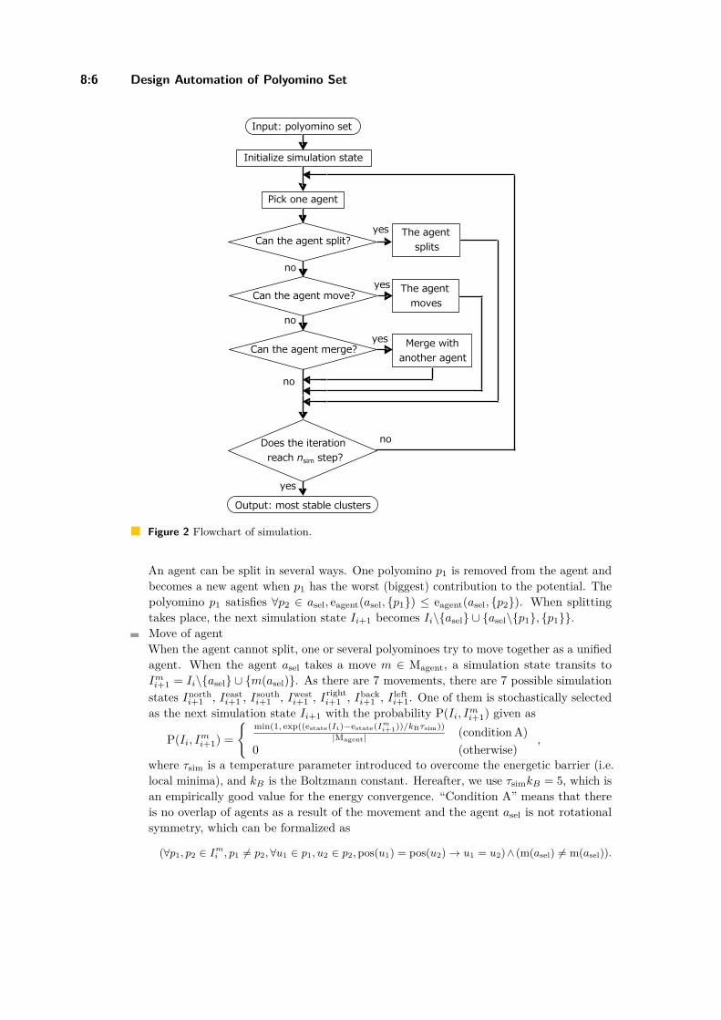
8:6 Design Automation of Polyomino Set
Figure 2 Flowchart of simulation.
An agent can be split in several ways. One polyomino p1 is removed from the agent andbecomes a new agent when p1 has the worst (biggest) contribution to the potential. Thepolyomino p1 satisfies ∀p2 ∈ asel, eagent(asel, p1) ≤ eagent(asel, p2). When splittingtakes place, the next simulation state Ii+1 becomes Ii\asel ∪ asel\p1, p1.Move of agentWhen the agent cannot split, one or several polyominoes try to move together as a unifiedagent. When the agent asel takes a move m ∈ Magent, a simulation state transits toImi+1 = Ii\asel ∪ m(asel). As there are 7 movements, there are 7 possible simulationstates Inorth
i+1 , Ieasti+1 , Isouth
i+1 , Iwesti+1 , Iright
i+1 , Ibacki+1 , I left
i+1. One of them is stochastically selectedas the next simulation state Ii+1 with the probability P(Ii, Imi+1) given as
P(Ii, Imi+1) =
min(1, exp((estate(Ii)−estate(Imi+1))/kBτsim))
|Magent| (condition A)0 (otherwise)
,
where τsim is a temperature parameter introduced to overcome the energetic barrier (i.e.local minima), and kB is the Boltzmann constant. Hereafter, we use τsimkB = 5, which isan empirically good value for the energy convergence. “Condition A” means that thereis no overlap of agents as a result of the movement and the agent asel is not rotationalsymmetry, which can be formalized as
(∀p1, p2 ∈ Imi , p1 6= p2, ∀u1 ∈ p1, u2 ∈ p2, pos(u1) = pos(u2)→ u1 = u2)∧ (m(asel) 6= m(asel)).

Y. Matsumura, I. Kawamata, and S. Murata 8:7
Merge of agentsIf all the possible movements increase the potential energy (i.e. ∀m ∈ Magent,P(Ii, Imi+1) <1/|Magent|) and also none of the movements are chosen by the calculated possibilities, theagent then try to merge with a neighboring agent. This condition implies that there is anattractive interaction between asel and the neighboring agent.The agent asel merges with another agent a1 that can make the assembly most stablein respect to the potential energy. The agent a1 satisfies ∀a2 ∈ Ii, eagent(asel, a1) ≤eagent(asel, a2). When the agent asel merges with the agent a1, the simulation statebecomes
Ii+1 = Ii\asel, a1 ∪ asel ∪ a1.
The most stable simulation state is predicted by iterating the above state transition fornsim times. When a polyomino species P is given, the resulting assembly is defined as a setof clusters A(P ) such that
A(P ) = cl(Ibest) (∃Ibest ∈ X,∀I ∈ X, estate(Ibest) ≤ estate(I)),
where X is the set of simulation state through the simulation (X = I0, I1, . . . , Insim).
3 Design automation
3.1 CriteriaBy using the simulation model in Section 2, we solve a shape self-assembly polyominoset (SAP) problem, which is formalized as follows.
The target assembly is given as a shape defined as a finite set of positions s =(x1, y1), (x2, y2), . . . with the size mshape = max(x1, x2, . . .) − min(x1, x2, . . .), andnshape = max(y1, y2, . . .)−min(y1, y2, . . .).If a polyomino species P can construct a shape s through self-assembly, then P is said tobe an polyomino species of s.The size of polyominoes in the polyomino species P is less than or equal to mpoly × npoly,and must be smaller than that of the target shape s.There are no limitations on the number of representative polyominoes |P | and glue types|Gl(P)|.An optimum polyomino species for a shape of finite size is the polyomino species ofminimum cardinality (i.e., with the smallest number of representative polyominoes).The SAP (shape self-assembly polyomino species) problem is defined as a problem to findthe optimum polyomino species for a given finite-size shape.
3.2 OutlineTo tackle the SAP problem, we employ a simulated-annealing algorithm which is one ofthe meta-heuristics approaches. The flowchart of the algorithm is given in Fig. 3. Aninitial polyomino species is randomly generated from a given shape s and evaluated bythe simulation. In our optimization strategy, a polyomino species is rated better when thepredicted assembly is closer to the target shape, and also the number of representativepolyominoes and the number of glue types are smaller. A polyomino species is graduallyimproved by repeating evolutionary process.
DNA 26
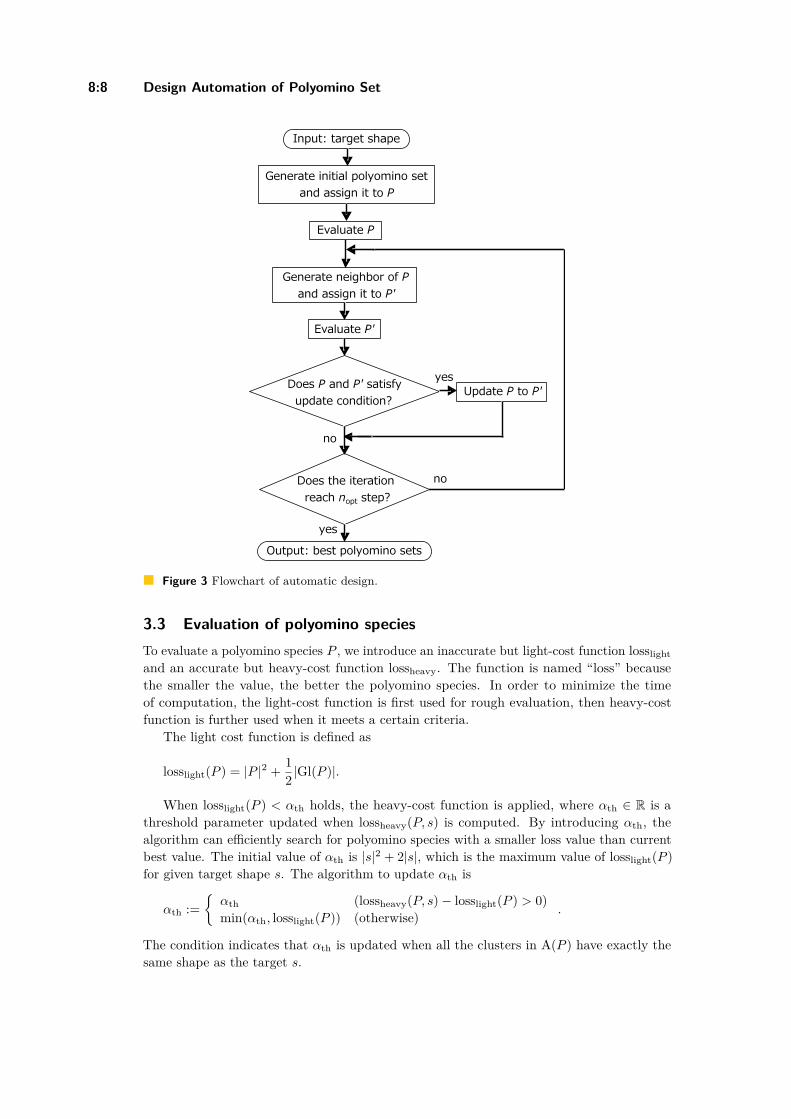
8:8 Design Automation of Polyomino Set
Figure 3 Flowchart of automatic design.
3.3 Evaluation of polyomino speciesTo evaluate a polyomino species P , we introduce an inaccurate but light-cost function losslightand an accurate but heavy-cost function lossheavy. The function is named “loss” becausethe smaller the value, the better the polyomino species. In order to minimize the timeof computation, the light-cost function is first used for rough evaluation, then heavy-costfunction is further used when it meets a certain criteria.
The light cost function is defined as
losslight(P ) = |P |2 + 12 |Gl(P )|.
When losslight(P ) < αth holds, the heavy-cost function is applied, where αth ∈ R is athreshold parameter updated when lossheavy(P, s) is computed. By introducing αth, thealgorithm can efficiently search for polyomino species with a smaller loss value than currentbest value. The initial value of αth is |s|2 + 2|s|, which is the maximum value of losslight(P )for given target shape s. The algorithm to update αth is
αth :=αth (lossheavy(P, s)− losslight(P ) > 0)min(αth, losslight(P )) (otherwise) .
The condition indicates that αth is updated when all the clusters in A(P ) have exactly thesame shape as the target s.
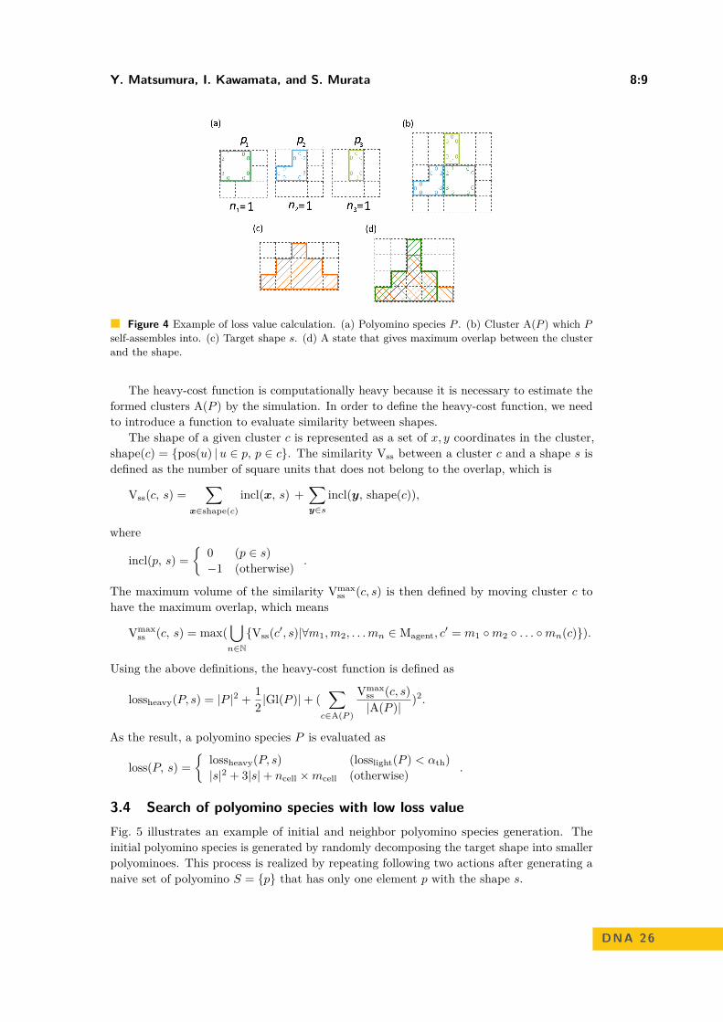
Y. Matsumura, I. Kawamata, and S. Murata 8:9
Figure 4 Example of loss value calculation. (a) Polyomino species P . (b) Cluster A(P ) which P
self-assembles into. (c) Target shape s. (d) A state that gives maximum overlap between the clusterand the shape.
The heavy-cost function is computationally heavy because it is necessary to estimate theformed clusters A(P ) by the simulation. In order to define the heavy-cost function, we needto introduce a function to evaluate similarity between shapes.
The shape of a given cluster c is represented as a set of x, y coordinates in the cluster,shape(c) = pos(u) |u ∈ p, p ∈ c. The similarity Vss between a cluster c and a shape s isdefined as the number of square units that does not belong to the overlap, which is
Vss(c, s) =∑
x∈shape(c)
incl(x, s) +∑y∈s
incl(y, shape(c)),
where
incl(p, s) =
0 (p ∈ s)−1 (otherwise) .
The maximum volume of the similarity Vmaxss (c, s) is then defined by moving cluster c to
have the maximum overlap, which means
Vmaxss (c, s) = max(
⋃n∈NVss(c′, s)|∀m1,m2, . . .mn ∈ Magent, c
′ = m1 m2 . . . mn(c)).
Using the above definitions, the heavy-cost function is defined as
lossheavy(P, s) = |P |2 + 12 |Gl(P )|+ (
∑c∈A(P )
Vmaxss (c, s)|A(P )| )2.
As the result, a polyomino species P is evaluated as
loss(P, s) =
lossheavy(P, s) (losslight(P ) < αth)|s|2 + 3|s|+ ncell ×mcell (otherwise) .
3.4 Search of polyomino species with low loss valueFig. 5 illustrates an example of initial and neighbor polyomino species generation. Theinitial polyomino species is generated by randomly decomposing the target shape into smallerpolyominoes. This process is realized by repeating following two actions after generating anaive set of polyomino S = p that has only one element p with the shape s.
DNA 26

8:10 Design Automation of Polyomino Set
Figure 5 Generation of initial polyomino species and neighbor polyomino species.
Action1A square unit u ∈ p is randomly selected. If randomly selected polyomino p ∈ S satisfies“condition B”, the algorithm removes the square unit u from the polyomino p and generatea new polyomino u. Here, condition B for a given polyomino p means that there areno other polyominoes with the same shape, or the size of p is smaller than or equal tomfix × nfix. The S is updated to S\p ∪ p\u, u. The probability to perform thisaction is rgen.Action2A pair of neighboring polyominoes p and p′ are randomly selected from S. If thepolyominoes p and p′ satisfy condition B, the algorithm removes a randomly selectedsquare unit u ∈ p from p that is adjacent to p′, and add it to p′. The S is updated toS\p, p′ ∪ p\u, p′ ∪ u. The probability to perform this action is 1− rgen.
If there are no polyominoes which meet condition B, one of these two actions takes placeignoring condition B. These two actions are repeated more than nnew steps, so that the sizesof all the polyominoes become smaller or equal to mpoly × npoly. Hereafter, we use mfix = 2and nfix = 1 and rgen = 0.05, nnew = 100.
Next, the algorithm assigns the glue types of polyominoes. Each glue type of polyominoesis set to all different value such that the square units have complementary glue types incontacting face with another polyomino. Glue types which are not contacting with anyother polyomino are fixed to 0. Polyominoes with the equivalent shape are converted toequivalent polyominoes by assigning glue types properly (see Appendix A.2). From the setof polyominoes, corresponding polyomino species can be trivially constructed.

Y. Matsumura, I. Kawamata, and S. Murata 8:11
To make a neighbor polyomino species, one of the two decomposing actions is applied asa mutation and then new glue types are assigned.
When the current polyomino species is P and its new neighbor is P ′, the possibility toaccept P ′ is
P(P, P ′) =
1 (loss(P, s)− loss(P ′, s) ≥ 0)exp((loss(P, s)− loss(P ′, s)) / τsa) (otherwise) ,
where τsa is a constant temperature parameter. Hereafter, we use τsa = 10, which empiricallyaccepts 20% of transitions that increase the loss values. The total iteration nopt is set to 100.
4 Result
To demonstrate the validity of proposed algorithm, we tested 3 target shapes with differentcomplexities (small, medium, and large), where mpoly and npoly are both set to 3. Foreach case, we run 100 searches for statistical analysis. The small target is given in 4 × 4lattice (Fig. 6(a)). For this target, reasonably good polyomino species were always obtainedsuch as the example in Fig. 6(b,c). The loss function development of 10 representativesearches are shown in Fig. 6(d). The average loss value over 100 searches was 12.5 with astandard deviation of ±0.37, which is smaller than 67.3± 14.6 of 100 random searches thatfind the best candidate from randomly generated 100 polyomino species.
Figure 6 (a) Target shape. (b) An example of polyomino species P . (c) Cluster which P
self-assembles into. (d) Development of loss function. The illustrated solution is shown in bold.
The medium target is given in a 5 × 5 lattice (Fig. 7(a)). A polyomino species thatself-assembles into the target shape was also found as expected (Fig. 7(b,c)). The averageloss value was 15.4± 2.7, which is significantly smaller than 134.2± 29.0 of random search.Ten representative results are shown in Fig. 7(d).
The large target is given in a 6× 6 lattice (Fig. 8(a)). Some of the searches succeeded infinding a polyomino species that self-assembles into the target shape as in the example ofFig. 8(b,c). The polyominoes in the set, however, were all different and none of them wererecycled in different places. The average loss value was 144.7± 87.7, which is smaller than201.0± 121.6 of random search. Ten representative results are shown in Fig. 8(d).
The performance of the proposed algorithm is summarized in Fig. 9. In the small andmedium cases, the loss values of proposed algorithm got significantly smaller than those ofrandom search. In the large case, however, the difference between the proposed algorithmand random search was not as significant. This may due to insufficient iteration of the
DNA 26

8:12 Design Automation of Polyomino Set
Figure 7 (a) Target shape. (b) An example of polyomino species P . (c) Cluster assembled by P .(d) Development of loss function. The illustrated solution is shown in bold.
Figure 8 (a) Target shape. (b) An example of polyomino species P . (c) Cluster assembled by P .(d) Development of loss function. The illustrated solution is shown in bold.
search. We further quantified the convergence speed of the search using a logarithmic fit.The development of loss values in respect to the logarithmic optimization step with estimatedslopes are shown in inset of Fig. 9(b). The number of iteration that is necessary to optimizethe polyomino species using our strategy may grow exponentially to the size of the target.
5 Discussion
In this paper, we consider the problem of finding minimum set of polyominoes that assembleinto a desired shape. A simulator developed on the agent-based Monte Carlo methodevaluates the potential energy among the polyominoes and updates the simulation state todecrease the total potential. Since the geometrical interactions between polyominoes haveto be taken into account, the developed simulator become complicated compared with thesimulators for homogeneous units such as kTAM, where a set of polyominoes is representedas an agent, which can move, merge, and split during the simulation. With this framework,a self-assembly processes of polyominoes can be efficiently simulated.
In the proposed algorithm, meta-heuristic method called simulated annealing was adopted.Because of the enormous search space for the design problem, a two-step evaluation strategywas adopted to prune unpromising solution spaces. Automatic design for three exampletargets with different size and complexity was tested to show the feasibility of the proposedmethod.

Y. Matsumura, I. Kawamata, and S. Murata 8:13
Figure 9 (a) The average of loss values at the last iteration of the searches of small (4 × 4),medium (5× 5), and large (6× 6) cases. The results of random search and proposed algorithms arecompared. (b) Convergence speed of the proposed algorithm using a logarithmic fit. The inset showsthe log-scale mean development of loss values, where standard deviation is illustrated as transparentarea. The bars summarize the estimated slopes in the log-scale graph. The algorithms are run 100times, and error bar indicates the standard deviation.
In order to solve a larger problem, we need to improve the efficiency of the algorithm,especially to reduce the computational cost of Monte Carlo simulation. For this purpose,it is necessary to redesign the potential energy between polyominoes to avoid kinetic traps.Introducing a new criterion to terminate the simulation at an appropriate step will be alsoeffective. Larger-scale problems can be solved by introducing parallel computing hardwaresuch as GPU along with the above improvements of the algorithms. From a computer sciencepoint of view, whether or not the automatic design problem of the polyomino set is NP is aninteresting issue. Also, extending the problem to three-dimensional polycube is remained fora future work.
References
1 Mika Göös and Pekka Orponen. Synthesizing minimal tile sets for patterned dna self-assembly. In International Workshop on DNA-Based Computers, pages 71–82. Springer, 2010.doi:10.1007/978-3-642-18305-8_7.
2 Yu He, Yi Chen, Haipeng Liu, Alexander E Ribbe, and Chengde Mao. Self-assembly ofhexagonal dna two-dimensional (2d) arrays. Journal of the American Chemical Society,127(35):12202–12203, 2005. doi:10.1021/ja0541938.
3 Chenxiang Lin, Yan Liu, Sherri Rinker, and Hao Yan. Dna tile based self-assembly: build-ing complex nanoarchitectures. ChemPhysChem, 7(8):1641–1647, 2006. doi:10.1002/cphc.200600260.
4 Xiaojun Ma and Fabrizio Lombardi. Synthesis of tile sets for dna self-assembly. IEEETransactions on Computer-Aided Design of Integrated Circuits and Systems, 27(5):963–967,2008. doi:10.1109/tcad.2008.917973.
5 Sung Ha Park, Robert Barish, Hanying Li, John H Reif, Gleb Finkelstein, Hao Yan, andThomas H LaBean. Three-helix bundle dna tiles self-assemble into 2d lattice or 1d templatesfor silver nanowires. Nano letters, 5(4):693–696, 2005. doi:10.1021/nl050108i.
6 Matthew J Patitz. An introduction to tile-based self-assembly and a survey of recent results.Natural Computing, 13(2):195–224, 2014. URL: https://link.springer.com/content/pdf/10.1007/s11047-013-9379-4.pdf.
DNA 26
8:14 Design Automation of Polyomino Set
7 Paul WK Rothemund. Folding dna to create nanoscale shapes and patterns. Nature,440(7082):297–302, 2006. doi:10.1038/nature04586.
8 Alessandro Troisi, Vance Wong, and Mark A Ratner. An agent-based approach for modelingmolecular self-organization. Proceedings of the National Academy of Sciences, 102(2):255–260,2005. doi:10.1073/pnas.0408308102.
9 Erik Winfree. Simulations of computing by self-assembly. In Fourth International Meeting onDNA-Based Computing. California Institute of Technology, 1998. doi:10.7907/Z9TB14X7.
10 Erik Winfree and Renat Bekbolatov. Proofreading tile sets: Error correction for algorithmicself-assembly. In International Workshop on DNA-Based Computers, pages 126–144. Springer,2003. doi:10.1007/978-3-540-24628-2_13.
11 Erik Winfree, Furong Liu, Lisa A Wenzler, and Nadrian C Seeman. Design and self-assemblyof two-dimensional dna crystals. Nature, 394(6693):539–544, 1998. doi:10.1038/28998.
12 Hao Yan, Sung Ha Park, Gleb Finkelstein, John H Reif, and Thomas H LaBean. Dna-templatedself-assembly of protein arrays and highly conductive nanowires. science, 301(5641):1882–1884,2003. doi:10.1126/science.1089389.
A Appendix
A.1 MovementsEach movement of the polyomino p is defined as
north(p) =⋃u∈p(coord(pos(u),N), gl(u)),
east(p) =⋃u∈p(coord(pos(u),E), gl(u)),
south(p) =⋃u∈p(coord(pos(u),S), gl(u)),
west(p) =⋃u∈p(coord(pos(u),W), gl(u)),
right(p) =⋃u∈p(−(posy(u)− cy(p)) + cx(p),posx(u)− cx(p) + cy(p), gl(u)|r),
back(p) =⋃u∈p(−(posx(u)− cx(p)) + cx(p), (posy(u)− cy(p)) + cy(p), gl(u)|b),
left(p) =⋃u∈p(posy(u)− cy(p) + cx(p),−(posx(u)− cx(p)) + cy(p), gl(u)|l),
where gl(u) is the glue types g of u = (x, y, g) and g|r, g|b, g|l are the glue types which canbe obtained by rotating g. Namely,
g|r(d) =
g(W) (d = N)g(N) (d = E)g(E) (d = S)g(S) (d = W)
,
g|b(d) =
g(S) (d = N)g(W) (d = E)g(N) (d = S)g(E) (d = W)
,

Y. Matsumura, I. Kawamata, and S. Murata 8:15
g|l(d) =
g(E) (d = N)g(S) (d = E)g(W) (d = S)g(N) (d = W)
.
Similarly, each movement of the agent a is defined as
north(a) =⋃p∈anorth(p),
east(a) =⋃p∈aeast(p),
south(a) =⋃p∈asouth(p),
west(a) =⋃p∈awest(p),
right(a) =⋃p∈a⋃u∈p(−(posy(u)− cy(p)) + cx(a),posx(u)− cx(a) + cy(a), gl(u)|r),
back(a) =⋃p∈a⋃u∈p(−(posx(u)− cx(a)) + cx(a),−(posy(u)− cy(a)) + cy(a), gl(u)|b),
left(a) =⋃p∈a⋃u∈p(posy(u)− cy(a) + cx(a),−(posx(u)− cx(a)) + cy(a), gl(u)|l),
where cx(a) and cy(a) are the center of mass of an agent a, which is defined as cx(a) =round(
∑u∈p,p∈a posx(u)/|a|) and cy(a) = round(
∑u∈p,p∈a posy(u)/|a|)).
A.2 Glue type assignmentGiven a naive set of polyominoes S, the assignment of glue types satisfies the conditions;
∀p1, p2 ∈ S, ∀u1 ∈ p1,∀u2 ∈ p2,∀d ∈ D, gl(u1, d) = 0→coord(pos(u1), d) 6= pos(u2), and
∀p1, p2 ∈ S, ∀u1 ∈ p1,∀u2 ∈ p2,∀d ∈ D, coord(pos(u), d) = pos(u2)→gl(u1, d)) + gl(u2, d) = 0 ∧ gl(u1, d)) 6= 0.
The first condition means that the glue type is 0 when there are no neighboring squareunits. The second condition guarantees that the the neighboring units have complementaryglue types. Finally, the number of representative polyominoes are decreased as much aspossible by assigning glue types through an ad-hoc trial and error. The assignment of gluetypes is applied to construct the initial and neighbor polyomino species.
DNA 26


scadnano: A Browser-Based, Scriptable Tool forDesigning DNA NanostructuresDavid Doty1
University of California, Davis, CA, USAhttps://web.cs.ucdavis.edu/~doty/[email protected]
Benjamin L LeeUniversity of California, Davis, CA, [email protected]
Tristan StérinMaynooth University, Irelandhttps://dna.hamilton.ie/tsterin/[email protected]
AbstractWe introduce scadnano (short for “scriptable cadnano”), a computational tool for designing syntheticDNA structures. Its design is based heavily on cadnano [24], the most widely-used software fordesigning DNA origami [33], with three main differences:
1. scadnano runs entirely in the browser, with no software installation required.2. scadnano designs, while they can be edited manually, can also be created and edited by a
well-documented Python scripting library, to help automate tedious tasks.3. The scadnano file format is easily human-readable. This goal is closely aligned with the scripting
library, intended to be helpful when debugging scripts or interfacing with other software. Theformat is also somewhat more expressive than that of cadnano, able to describe a broader rangeof DNA structures than just DNA origami.
2012 ACM Subject Classification Applied computing → Computer-aided design
Keywords and phrases computer-aided design, structural DNA nanotechnology, DNA origami
Digital Object Identifier 10.4230/LIPIcs.DNA.2020.9
Supplementary Material stable/dev apps: https://scadnano.org, https://scadnano.org/devrepositories: https://github.com/UC-Davis-molecular-computing/scadnanohttps://github.com/UC-Davis-molecular-computing/scadnano-python-packagePython library API: https://scadnano-python-package.readthedocs.iotutorials: https://github.com/UC-Davis-molecular-computing/scadnano-python-package/blob/master/tutorial/tutorial.md, https://github.com/UC-Davis-molecular-computing/scadnano/blob/master/tutorial/tutorial.md
Funding David Doty: Supported by NSF grants 1619343, 1900931, and CAREER grant 1844976.Benjamin L Lee: Supported by REU supplement through NSF CAREER grant 1844976.Tristan Stérin: Supported by European Research Council (ERC) under the European Union’sHorizon 2020 research and innovation programme (grant agreement No 772766, Active-DNA project),and Science Foundation Ireland (SFI) under Grant number 18/ERCS/5746.
Acknowledgements We thank Matthew Patitz for beta-testing and feedback, and Pierre-ÉtienneMeunier, author of codenano, for valuable discussions regarding the data model/file format. We aregrateful to anonymous reviewers whose detailed feedback has increased the presentation quality.
1 Corresponding author
© David Doty, Benjamin L Lee, and Tristan Stérin;licensed under Creative Commons License CC-BY
26th International Conference on DNA Computing and Molecular Programming (DNA 26).Editors: Cody Geary and Matthew J. Patitz; Article No. 9; pp. 9:1–9:17
Leibniz International Proceedings in InformaticsSchloss Dagstuhl – Leibniz-Zentrum für Informatik, Dagstuhl Publishing, Germany

9:2 scadnano: A Browser-Based, Scriptable Tool for Designing DNA Nanostructures
1 Introduction
1.1 DNA origami and cadnanoSince its inception almost 15 years ago, DNA origami [33] has stood as the most reliable,high-yield, and low-cost method for synthesizing uniquely addressed DNA nanostructures,on the order of 100 nm wide, with ≈ 6 nm addressing resolution (i.e., that’s how far apartindividual strands are).2 To create the original designs, Rothemund wrote custom Matlabscripts to generate and visualize the designs (with ASCII art). Soon after, the softwarecadnano was developed by Douglas et al. [24], as part of a project extending the original 2DDNA origami results to 3D structures [23]. cadnano has become a standard tool in structuralDNA nanotechnology, used for describing most major DNA origami designs.
1.2 scadnanoThe scadnano graphical interface is shown in Figure 1; it mimics that of cadnano.
The goal of scadnano is to aid in designing large-scale DNA nanostructures, such asDNA origami, with ability to edit structures either manually, or programmatically througha scripting library. scadnano seeks to imitate most of the features of cadnano, with threemajor differences that enhance the usability and interoperability of scadnano:1. scadnano runs entirely in the browser, with no software installation required. It aims,
above all else, to be simple and easy to use, well-suited for teaching, for example.2. scadnano designs, while they can be edited manually, can also be created and edited by a
well-documented Python scripting library, to help automate tedious tasks.33. The scadnano file format is easily human-readable and expressive, natural for describing
a broader range of DNA structures than just DNA origami. This goal is closely alignedwith the scripting library, useful when debugging scripts or interfacing with other soft-ware. A related project, codenano [5], uses essentially the same file format, developedsimultaneously in consultation with the main author of codenano.
The major features of scadnano are described in more detail in Section 3. Designed withinteroperability in mind, any cadnano design can be imported into scadnano, and scadnanodesigns obeying certain constraints (see Section 2.3) can be exported to cadnano.
1.3 Related workcadnano is the most related prior work, and its design was the inspiration for scadnano.Section 3.1 goes into detail about features that scadnano shares in common with cadnano,and the rest of Section 3 discusses some extra features in scadnano. codenano is close inpurpose to scadnano [5], being also browser-based and scriptable. Unlike scadnano, codenanoincludes 3D visualisation components but not graphical editing.
2 The basic idea of DNA origami is to use a long scaffold strand (either synthesized or natural; the mostcommon choice is the natural circular single-stranded virus known as M13mp18, 7249 bases long), andto synthesize shorter (a few dozen bases long) staple strands designed to bind to multiple regions of thescaffold. Upon mixing in standard DNA self-assembly buffer conditions (e.g., 10 mM Tris, 1 mM EDTA,pH 8.0, 12.5 mM MgCl2), with staples “significantly” more concentrated than the scaffold (typicalconcentrations are 1 nM scaffold and 10 nM each staple), and annealing from 90°C to 20°C for one hour,the staples bind to the scaffold and fold it into the desired shape, while excess staples remain free insolution and are easily separated from the formed structures by standard purification techniques.
3 cadnano v2.5 has a Python scripting library, but its documentation is incomplete [3], and cadnano v2.5has not been updated for two years [2] at the time of this writing.

D. Doty, B. L. Lee, and T. Stérin 9:3
Figure 1 screenshot of scadnano, annotated with some labels (in orange rectangles) to pointout various parts of the data model.4 The center part is the main view, which shows the x and y
coordinates; most editing takes place here. On the left is the side view, which shows the z and y
coordinates. y increases going down in both views (so-called “screen coordinates), x increases goingright in the main view and going into the screen in the side view. z increases going right in the sideview and going out of the screen in the main view. The Edit modes on the right change what sortsof edits are possible, and the Select modes change what sort of objects can be selected while in the“select” edit mode.
vHelix [18] offers comprehensive 3D origami editing and visualisation features but relies onAutodesk Maya. Adenita [21] is a design and visualisation tool that allows one to work withvarious DNA nanostructures: standard parallel-helix DNA origami, wireframe origamis [28],and tile-based designs. Adenita is distributed within the SAMSON [17] molecular modelingplatform. Specific to the domain of 2D and 3D wireframe origamis, ATHENA [28] providesboth an editing interface and sequence design algorithms that generate staple sequences from a2D sketch. Not related to graphical or script-based DNA design editing, the following softwareprovides structural prediction tools for various features of DNA designs: CanDo [4] (finiteelements-based 3D structure prediction), NUPACK and ViennaRNA [30,43] (thermodynamicenergy of DNA strands), oxDNA [38] (kinetics prediction by molecular dynamics simulation),and MrDNA [31] (3D structure and kinetics prediction).
1.4 Paper outlineSection 2 describes the data model used by scadnano to represent a DNA design, andits closely related storage file format, including a comparison with cadnano’s file format.Section 3 describes several features of scadnano, including some that are absent from cadnano.Section 4 explains the software architecture of scadnano. Section 4 is not necessary tounderstand how to use scadnano, but it helps to justify why scadnano may be simpler tomaintain and enhance in the future. Section 5 discusses possible future features.
This paper is not a self-contained document describing scadnano in full. See the supple-mentary material links for online documentation, tutorials, and the Python library API.
4 This design is intended merely to show some scadnano features, not to show proper design respectingDNA crossover geometry; it would be strained if actually assembled.
DNA 26
9:4 scadnano: A Browser-Based, Scriptable Tool for Designing DNA Nanostructures
2 Data model and file format
2.1 scadnano data model
Although scadnano and its data model are natural for describing DNA origami, it can beused to describe any DNA nanostructure composed of several DNA strands. Like cadnano,scadnano is especially well-suited to structures where all DNA helices are parallel, whichincludes not only origami, but also certain tile-based designs (e.g., [39,40,42]), or “criss-crossslat” assembly [32]. The basic concepts, explained in more detail below, are that the designis composed of several strands, which are bound to each other on some domains, and possiblysingle-stranded on others, and double-stranded portions of DNA occupy a helix.
DNA Design
An example DNA design is shown in Figure 1, showing most of the features discussed here.A design (the type of object stored in a .sc file produced when clicking “Save” in scadnano)consists of a grid type (a.k.a., lattice, one of the following types: square, honeycomb, hex, ornone, explained below), a list of helices, and a list of strands. The order of strands in thelist generally doesn’t matter, although it influences which are drawn on top, so a strand laterin the list will have its crossovers drawn over the top of earlier strands.
Helices
Unlike strands, the order of the helices matters; if there are h helices, the helices are numbered0 through h − 1. This can be overridden by specifying a field called idx in each helix, butthe default is to number them consecutively. Each helix defines a set of integer offsets with aminimum and maximum; in the example above, the minimum and maximum for each helixare 0 and 48, respectively, so 48 total offsets are shown. Each offset is a position where aDNA base of a strand can go.
Helices in a grid (meaning one of square, honeycomb, or hex) have a 2D integergrid_position depicted in the side view (see Figure 3). Helices without a grid (mean-ing grid type none) have a position, a 3D real vector describing their x, y, z coordinates.Each Helix also has fields to describe angular orientation, using the “aircraft principleaxes” pitch, roll, and yaw (default 0), although this feature is currently not well-supported(https://github.com/UC-Davis-molecular-computing/scadnano/issues/39). The co-ordinates of helices in the main view depends on grid_position if a grid is used, and onposition otherwise. (Each grid position is essentially interpreted as a position with z =pitch = roll = yaw = 0.) Helices are listed from top to bottom in the order they appear inthe sequence, unless the property helices_view_order is specified in the design to displaythem in a different order, though currently this can only be done in the scripting library.
Helix.roll describes the DNA backbone rotation about the long axis of the helix. Atthe offset Helix.min_offset, the backbone of the forward strand on that helix has angleHelix.roll, where we define 0 degrees to point to straight up in the side view. Rotation isclockwise as the rotation increases from 0 up to 360 degrees. This feature is not intendedas a globally predictive model of stability. Rather, it helps visualize backbone angles, toplace crossovers that minimize strain, by ensuring crossovers are “locally consistent”, withoutenforcing a global notion of absolute backbone rotation on all offsets in the system.

D. Doty, B. L. Lee, and T. Stérin 9:5
Strands and domains
Each strand is defined primarily by an ordered list of domains. Each domain is either asingle-stranded loopout not associated to any helix, or it is a bound domain: a region of thestrand that is contiguous on a single helix. The phrase is a bit misleading, since a bounddomain is not necessarily bound to another strand, but the intention is for most of them tobe bound, and for single-stranded regions usually to be represented by loopouts.
Each bound domain is specified by four mandatory properties: helix (indicating theindex of the helix on which the domain resides), forward (a direction can be forward orreverse, indicated by whether this field is true or false), start integer offset, and a largerend integer offset. As with common string/list indexing in programming languages, startis inclusive but end is exclusive. So for example, a bound domain with end=8 is adjacentto one with start=8. In the main view, forward bound domains are depicted on the tophalf of the helix, and reverse (those with forward=false) are on the bottom half. If a bounddomain is forward, then start is the offset of its 5’ end, and end−1 is the offset of its 3’ end,otherwise these roles are reversed. There is implicitly a crossover between adjacent bounddomains in a strand. Loopouts are explicitly specified as a (non-bound) domain in betweentwo bound domains. Currently, two loopouts cannot be consecutive (and this will remaina requirement), and a loopout cannot be the first or last domain of a strand (this may berelaxed in the future).
Bound domains may have optional fields, notably deletions (called skips in cadnano) andinsertions (called loops in cadnano). They are a visual trick used to allow bound domainsto appear to be one length in the main view of scadnano, while actually having a differentlength. Normally, each offset represents a single base. If instead a deletion appears at thatoffset, then it does not correspond to any DNA base. If an insertion appears at that offset, ithas a positive integer length: the number of bases represented by that offset is length+1.
Strand optional fields
Each strand also has a color and a Boolean field is_scaffold. DNA origami designs have atleast one strand that is a scaffold (but can have more), and a non-DNA-origami design issimply one in which every strand has is_scaffold = false. Unlike cadnano, a scaffold strandcan have either direction on any helix. When there is at least one scaffold, all non-scaffoldstrands are called staples. The general idea behind DNA origami is that all binding is betweenscaffolds and staples, never scaffold-scaffold or staple-staple. However, this convention is notenforced by scadnano; there are legitimate reasons for non-scaffold strands to bind to eachother (e.g., DNA walkers [26] or circuits [20] on the surface of an origami).
A strand can have an optional DNA sequence. Of course, since the whole point of thissoftware is to help design DNA structures, at some point a DNA sequence should be assignedto some of the strands. However, it is often best to mostly finalize the design before assigninga DNA sequence, which is why the field is optional. Many of the operations attempt to keepthings consistent when modifying a design where some strands already have DNA sequencesassigned, but in some cases it’s not clear what to do. (e.g., what DNA sequence results whena length-5 strand with sequence AACGT is extended to be longer?)
DNA modifications
DNA modifications describe ways that various small molecules may be attached to syntheticDNA as part of the DNA synthesis process. Common DNA modifications include biotin(useful for binding to the protein streptavidin) and fluorophores such as Cy3 (useful for lightmicroscopy). Modifications can be attached to the 5’ end, the 3’ end, or to an internal base.
DNA 26
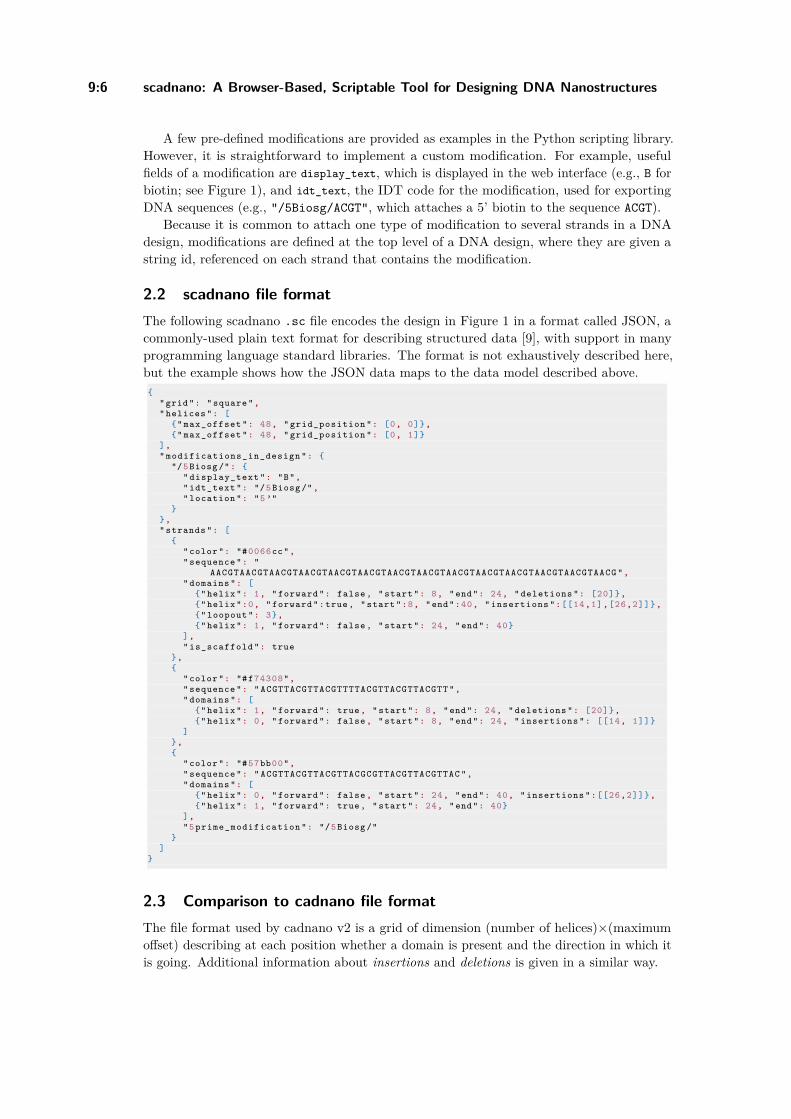
9:6 scadnano: A Browser-Based, Scriptable Tool for Designing DNA Nanostructures
A few pre-defined modifications are provided as examples in the Python scripting library.However, it is straightforward to implement a custom modification. For example, usefulfields of a modification are display_text, which is displayed in the web interface (e.g., B forbiotin; see Figure 1), and idt_text, the IDT code for the modification, used for exportingDNA sequences (e.g., "/5Biosg/ACGT", which attaches a 5’ biotin to the sequence ACGT).
Because it is common to attach one type of modification to several strands in a DNAdesign, modifications are defined at the top level of a DNA design, where they are given astring id, referenced on each strand that contains the modification.
2.2 scadnano file formatThe following scadnano .sc file encodes the design in Figure 1 in a format called JSON, acommonly-used plain text format for describing structured data [9], with support in manyprogramming language standard libraries. The format is not exhaustively described here,but the example shows how the JSON data maps to the data model described above.
"grid": " square "," helices ": [
" max_offset ": 48, " grid_position ": [0, 0]," max_offset ": 48, " grid_position ": [0, 1]
]," modifications_in_design ":
"/5 Biosg /": " display_text ": "B"," idt_text ": "/5 Biosg /"," location ": "5 ’"
," strands ": [
" color ": "#0066cc"," sequence ": "
AACGTAACGTAACGTAACGTAACGTAACGTAACGTAACGTAACGTAACGTAACGTAACGTAACGTAACG "," domains ": [
" helix ": 1, " forward ": false , " start ": 8, "end": 24, " deletions ": [20]," helix ":0, " forward ":true, " start ":8, "end":40, " insertions ":[[14,1],[26,2]]," loopout ": 3," helix ": 1, " forward ": false , " start ": 24, "end": 40
]," is_scaffold ": true
,
" color ": "#f74308"," sequence ": " ACGTTACGTTACGTTTTACGTTACGTTACGTT "," domains ": [
" helix ": 1, " forward ": true, " start ": 8, "end": 24, " deletions ": [20]," helix ": 0, " forward ": false , " start ": 8, "end": 24, " insertions ": [[14, 1]]
],
" color ": "#57bb00"," sequence ": " ACGTTACGTTACGTTACGCGTTACGTTACGTTAC "," domains ": [
" helix ": 0, " forward ": false , " start ": 24, "end": 40, " insertions ":[[26,2]]," helix ": 1, " forward ": true, " start ": 24, "end": 40
],"5 prime_modification ": "/5 Biosg /"
]
2.3 Comparison to cadnano file formatThe file format used by cadnano v2 is a grid of dimension (number of helices)×(maximumoffset) describing at each position whether a domain is present and the direction in which itis going. Additional information about insertions and deletions is given in a similar way.
D. Doty, B. L. Lee, and T. Stérin 9:7
An important goal of scadnano is to ensure interoperability with cadnano (see Section 3.9).Thus every cadnano design can be imported into scadnano. However, the converse is nottrue; scadnano’s data model can describe features not present in cadnano.
1. cadnano does not have a way to encode loopouts, modifications, or gridless designs.2. cadnano does not store DNA sequences in its file format.3. cadnano has the constraint that helices with even index have the scaffold going forward
and helices with odd index have the scaffold going backward. scadnano designs notfollowing that convention cannot be encoded in cadnano.
4. cadnano does not explicitly encode the grid type, instead inferring it from the maximumhelix offset: multiples of 21 represent the honeycomb grid, while multiples of 32 representthe square grid. To encode a scadnano design in cadnano’s convention, each helix’smaximum offset is modified to the lowest multiple of 21 or 32 fitting the design.
Converting a scadnano design to cadnano v2 is straightforward: lay out all domains of allstrands in a (number of helices)×(modified maximum offset) grid. Maximum offsets have tobe modified because of Item 4. However, converting a cadnano design to scadnano format isa bit more involved, requiring a connected components detection algorithm performed onthe grid – similar to a depth-first search – in order to identify strands and their domains.
3 Features
3.1 Features shared with cadnano v2The web interface of scadnano is similar to cadnano (see Figure 1). Like cadnano, scadnanois optimal for structures consisting of parallel helices. On the left, the side view shows across-sectional view of the lattice where helices can be added to the design. The main viewshows what the helix would look like going from left to right in the screen. Moving to theright in the main view is like moving “into the screen” in the side view.
DNA designs are drawn as they are often drawn in figures, with strands on a double-helixrepresented as straight lines that are connected to other helices by crossovers. Users can alsoadd deletions and insertions (called skips and loops in cadnano) which means a strand hasfewer or more bases than the interface’s visually depicted length. Insertions and deletionshelp to use a regular spacing pattern – note the “major tick marks” every 8 bases on thehelix – while allowing short regions to deviate and use more or fewer than the typical numberof bases between two major tick marks. One feature scadnano adds to cadnano is the abilityto customize the major tick marks, including non-regular spacing, e.g, alternating 10, 11, 10,11 for single-stranded tiles [39,42].
scadnano includes several “Edit modes”, many similar to those of cadnano, shown in thetop right corner of Figure 1. There are two main modes for editing, select mode and pencilmode, as well as several others explained in more detail in the scadnano documentation.Select mode allows users to select, resize, and delete items, just like in cadnano. (scadnanoadditionally allows users to copy and paste or move items; see Section 3.2). Pencil mode isused to create new objects such as helices, strands, or crossovers.
Users can assign DNA sequences to strands, and the complementary sequences for thebound strands are automatically computed. The common M13 DNA sequence is provided asa default for single-scaffold designs.
Although scadnano currently provides no 3D visualization, it does provide a primitive wayto visualize the DNA backbone angles to help pick where to place crossovers; see Figure 2.This feature is slightly more flexible than the analogous feature in cadnano in that the user
DNA 26

9:8 scadnano: A Browser-Based, Scriptable Tool for Designing DNA Nanostructures
(a) Backbone angles at a cros-sover.
(b) Backbone angle 3 bases tothe left.
Figure 2 The side view displays the backbone angles to aid with crossover placement.
is allow to set the backbone angle at one base position to see what that implies about thebackbone angle at other (typically nearby) base positions. For example, a user can “unstrain”the backbone at a crossover so that the backbone angles are perfectly aligned (see Figure 2a).The backbone angles at other positions are automatically computed (see Figure 2b).
The side and main view designs can be exported as SVG figures, and DNA sequences canbe be exported into a CSV file, as well as formats recognized by the synthesis company IDT.
0,01,0
2,0-1,0
-1,1
0,-1-1,-1 1,-1
2,-13,-1
4,-1
3,04,0
0,11,1
2,13,1
4,1
0,2-1,2 1,2
2,23,2
4,2
-1,30,3
1,32,3
3,34,3
-1,40,4
1,42,4
3,44,4
(a) Honeycomb grid, in-teger coordinates.
0,0 1,0 2,0-1,0
-1,1
0,-1-1,-1 1,-1 2,-1 3,-1 4,-1
3,0 4,0
0,1 1,1 2,1 3,1 4,1
0,2-1,2 1,2 2,2 3,2 4,2
-1,3 0,3 1,3 2,3 3,3 4,3
-1,4 0,4 1,4 2,4 3,4 4,4
(b) Square grid, integer co-ordinates.
(c) No grid, real-valued co-ordinates in units of nanomet-ers (coordinates not shown).
Figure 3 scadnano grids (hex grid not shown).
Like cadnano, helices can be placed in a square or honeycomb lattice, as shown inFigure 3a and Figure 3b. scadnano provides two more grids not available on cadnano: thehex grid (allowing helices in the “holes” of the honeycomb grid) and no grid; see Section 3.8.
The remainder of Section 3 describes features not shared with cadnano v2.
3.2 Copy and paste
A full DNA origami design using a standard 7249-base M13mp18 scaffold uses ≈ 200 staples,which are tedious to create manually. In scadnano, this process is accelerated by the

D. Doty, B. L. Lee, and T. Stérin 9:9
0
1
2
3
4
5
6
7
8
9
10
11
12
13
14
15
16
17
18
19
20
21
22
23
Figure 4 A standard 24 helix DNA origami rectangle design, with “twist-correction” [41].
copy/paste feature.5 For instance, to create a vertical “column” of 24 staples in a 24-helixrectangle (see Figure 4), one would create 2 types of staples (plus some special cases nearthe top/bottom), copy/paste them to make 4, copy/paste those to make 8, then copy/pastethe group of 8 two more times for a total of 24 staples. Since most of the design consistsof horizontally translated copies of this column, it can be created quickly by copying andpasting the column.
3.3 Scripting libraryThe scadnano Python module allows one to write scripts for creating and editing scadnanodesigns. (Note that cadnano v2.5, unlike v2, does have a scripting library [2], though withincomplete documentation.) The module helps automate some of the tedious tasks involvedin creating DNA designs, as well as making large-scale changes to them that are easier todescribe programmatically than to do by hand in scadnano.
For example, the following is Python code generating the design in Figure 4, creating a.sc file with the design and a Microsoft Excel file with staple strand DNA sequences in aformat ready to order from the DNA synthesis company IDT. It is perhaps unnecessary toread the code in detail; we provide it to demonstrate that “production-ready” designs canbe created with relatively short and simple scripts. It follows the pattern described in theonline tutorial (see first page).
5 cadnano provides features to make large designs quickly, autostaple and autobreak, which are faster thancopy/pasting strands, though they give less control over the outcome.
DNA 26

9:10 scadnano: A Browser-Based, Scriptable Tool for Designing DNA Nanostructures
import scadnano as sc
def create_design ():design = create_design_with_precursor_scaffolds ()add_scaffold_nicks ( design )add_scaffold_crossovers ( design )scaffold = design . strands [0]scaffold . set_scaffold ()add_precursor_staples ( design )add_staple_nicks ( design )add_staple_crossovers ( design )add_twist_correcting_deletions ( design )design . assign_m13_to_scaffold ()return design
def create_design_with_precursor_scaffolds () -> sc. DNADesign :helices = [sc. Helix ( max_offset =304) for _ in range (24)]scaffolds = [sc. Strand ([ sc. Domain ( helix =helix , forward = helix %2 == 0, start =8, end=296) ])
for helix in range (24)]return DNADesign ( helices =helices , strands =scaffolds , grid= square )
def add_scaffold_nicks ( design : sc. DNADesign ):for helix in range (1, 24):
design . add_nick ( helix =helix , offset =152 , forward = helix %2 == 0)
def add_scaffold_crossovers ( design : sc. DNADesign ):crossovers = []for helix in range (1, 23, 2): # scaffold interior
crossovers . append (sc. Crossover ( helix1 =helix , helix2 = helix +1, offset1 =152 , forward1 = False ))
for helix in range (0, 23, 2): # scaffold edgescrossovers . append (
sc. Crossover ( helix1 =helix , helix2 = helix +1, offset1 =8, forward1 =True , half=True))
crossovers . append (sc. Crossover ( helix1 =helix , helix2 = helix +1, offset1 =295 , forward1 =True ,half=
True))design . add_crossovers ( crossovers )
def add_precursor_staples ( design : sc. DNADesign ):staples = [sc. Strand ([ sc. Domain ( helix =helix , forward = helix %2 == 1, start =8, end=296) ])
for helix in range (24)]for staple in staples :
design . add_strand ( staple )
def add_staple_nicks ( design : sc. DNADesign ):for helix in range (24):
start_offset = 32 if helix % 2 == 0 else 48for offset in range ( start_offset , 280 , 32):
design . add_nick (helix , offset , forward = helix %2 == 1)
def add_staple_crossovers ( design : sc. DNADesign ):for helix in range (23):
start_offset = 24 if helix % 2 == 0 else 40for offset in range ( start_offset , 296 , 32):
if offset != 152: # skip crossover near seamdesign . add_full_crossover ( helix1 =helix , helix2 = helix + 1,
offset1 =offset , forward1 = helix % 2 == 1)
def add_twist_correcting_deletions ( design : sc. DNADesign ):for helix in range (24):
for offset in range (27 , 294 , 48):design . add_deletion (helix , offset )
def export_idt_plate_file ( design : sc. DNADesign ):for strand in design . strands :
if strand != design . scaffold :strand . set_default_idt ( use_default_idt =True)
design . write_idt_plate_excel_file ( use_default_plates =True)
if __name__ == " __main__ ":design = create_design ()export_idt_plate_file ( design )design . write_scadnano_file ()
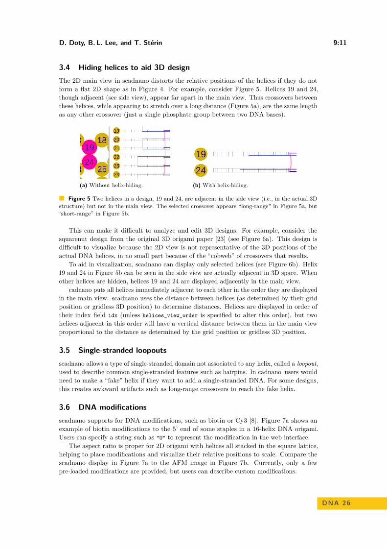
D. Doty, B. L. Lee, and T. Stérin 9:11
3.4 Hiding helices to aid 3D designThe 2D main view in scadnano distorts the relative positions of the helices if they do notform a flat 2D shape as in Figure 4. For example, consider Figure 5. Helices 19 and 24,though adjacent (see side view), appear far apart in the main view. Thus crossovers betweenthese helices, while appearing to stretch over a long distance (Figure 5a), are the same lengthas any other crossover (just a single phosphate group between two DNA bases).
(a) Without helix-hiding. (b) With helix-hiding.
Figure 5 Two helices in a design, 19 and 24, are adjacent in the side view (i.e., in the actual 3Dstructure) but not in the main view. The selected crossover appears “long-range” in Figure 5a, but“short-range” in Figure 5b.
This can make it difficult to analyze and edit 3D designs. For example, consider thesquarenut design from the original 3D origami paper [23] (see Figure 6a). This design isdifficult to visualize because the 2D view is not representative of the 3D positions of theactual DNA helices, in no small part because of the “cobweb” of crossovers that results.
To aid in visualization, scadnano can display only selected helices (see Figure 6b). Helix19 and 24 in Figure 5b can be seen in the side view are actually adjacent in 3D space. Whenother helices are hidden, helices 19 and 24 are displayed adjacently in the main view.
cadnano puts all helices immediately adjacent to each other in the order they are displayedin the main view. scadnano uses the distance between helices (as determined by their gridposition or gridless 3D position) to determine distances. Helices are displayed in order oftheir index field idx (unless helices_view_order is specified to alter this order), but twohelices adjacent in this order will have a vertical distance between them in the main viewproportional to the distance as determined by the grid position or gridless 3D position.
3.5 Single-stranded loopoutsscadnano allows a type of single-stranded domain not associated to any helix, called a loopout,used to describe common single-stranded features such as hairpins. In cadnano users wouldneed to make a “fake” helix if they want to add a single-stranded DNA. For some designs,this creates awkward artifacts such as long-range crossovers to reach the fake helix.
3.6 DNA modificationsscadnano supports for DNA modifications, such as biotin or Cy3 [8]. Figure 7a shows anexample of biotin modifications to the 5’ end of some staples in a 16-helix DNA origami.Users can specify a string such as "O" to represent the modification in the web interface.
The aspect ratio is proper for 2D origami with helices all stacked in the square lattice,helping to place modifications and visualize their relative positions to scale. Compare thescadnano display in Figure 7a to the AFM image in Figure 7b. Currently, only a fewpre-loaded modifications are provided, but users can describe custom modifications.
DNA 26

9:12 scadnano: A Browser-Based, Scriptable Tool for Designing DNA Nanostructures
(a) All helices shown, causing the dreaded crossover cobweb, like laser beams guarding priceless art.
(b) Restricted subset of helices displayed: only relevant helices and crossovers are shown.
Figure 6 Squarenut 3D origami [23], a typical 3D origami difficult to visualize in a 2D projection.
3.7 Unused fields
In order to maximize interoperability with other tools, scadnano allows arbitrary fields tobe included in a scadnano .sc file. Any fields that it does not recognize are simply ignored.However, they are stored and written back out when the file is saved. Thus, “light” editingof scadnano files is possible that will preserve fields used by other programs. For example,codenano [5] allows an optional field label on each strand, which will be preserved for eachstrand by scadnano while editing other aspects of the design.
3.8 Gridless helix placement
scadnano includes the option to use no grid; see Figure 3c. This allows more flexible helixplacement, where helix centers can be placed at any real-valued (i.e., floating-point) (z, y)coordinate. This feature is useful for some designs that do not align nicely with the standardsquare or honeycomb lattice. In the absence of a grid, coordinates of helices are specified innanometers. By default, the distance between each DNA helix center is 3 nm.6
6 The accepted measurement of the DNA double-helix diameter is ≈ 2 nm. However, AFM images showthat in 2D square-lattice DNA origami designs, an origami with n helices will have height in nanometersof approximately 3 · n due to electrostatic repulsion between neighboring helices.

D. Doty, B. L. Lee, and T. Stérin 9:13
0
1
2
3
4
5
6
7
8
9
10
11
12
13
14
151 1 1 1 1 1
1 1 1 1 1 1
1 1 1 1 1 1
1 1 1 1 1 1
1 1 1 1 1 1
1 1 1 1 1 1
1 1 1 1 1 1
1 1 1 1 1 1
1 1 1 1 1 1
1 1 1 1 1 1 1 1 1 1 1 1
1 1 1 1 1 1
1 1 1 1 1 1
1 1 1 1 1 1
1 1 1 1 1 1
1 1 1 1 1 1
1 1 1 1 1 1
1 1 1 1 1 1
1 1 1 1 1 1
1 1 1 1 1 1
1
1
1 O1
1
1
1
1O1
1
1
1
1
1
1
1
1
O1
OO1
O1
1
1
1
1O1
1
1
1
1
1
O
1
1O1OO
1O1
1
1
1
1
1
O
1
1
1
1O1
1
1
O1
OO1
O1
1
1
1
1
1
1
1
O1
OO1
O1
1
O1
1O
1O1
1
1
1
1
1
1
1
1
1
1
1
1
1
1
1
1
1
1
1
1
1
1
1
1
1
1
1
1
1O1
1
1
1
1
1
O
1O
1O1O
1
1O 1
1
1
O1
1
O
1
1
1
O1O1
1
1
1
1
1
(a) biotin DNA modifications on the 5’ end of some staples, displayed in scadnano.
(b) The same design imaged with atomic force microscopy (AFM), with strep-tavidin added to visualize the biotin locations. (scale bar: 50 nm) (image source:https://web.cs.ucdavis.edu/~doty/papers/#proposal)
Figure 7 An example of a design containing biotin modifications.
3.9 Interoperability with cadnanoInteroperability with cadnano (version 2) is an important goal of the project. Both thescadnano GUI and Python module provide functionality that allows users to import/exporta design from/to cadnano. All cadnano (version 2) designs can be imported in scadnano.However, because of fundamental differences between the way cadnano and scadnano encodedesigns, some scadnano designs cannot be converted cadnano (see Section 2.3).7
4 Software architecture
4.1 Two codebasesThe codebase for scadnano is split into two pieces: the Python scripting library, and theweb interface. Unfortunately, some algorithmic functionality is duplicated between them.We chose Python as the scripting language because it is easy to learn and already familiarto many physical scientists likely to use scadnano. However (despite innovations such asPyodide [11], Skulpt [15], and Brython [1]), Python is not well-suited for front-end webprogramming, where the code is executed in the browser rather than on a server. A designgoal of scadnano is to do as much work as possible in the browser.
The web interface is instead implemented using the Dart programming language [6], amodern, strongly-typed, object-oriented language that can be compiled to Javascript, thelingua franca of web browsers. In order to make the Python scripting library as easy to useas possible (no dependence on Dart libraries) and to keep the web interface as fast as possible
7 These constraints are described in the documentation: https://scadnano-python-package.readthedocs.io/en/latest/index.html#interoperability-cadnano-v2
DNA 26

9:14 scadnano: A Browser-Based, Scriptable Tool for Designing DNA Nanostructures
and avoid the need to farm out computation to a server, some algorithms (e.g., computingcomplementary DNA sequences of strands when they are bound to another strand that hashad a DNA sequence assigned to it) are implemented in both libraries.
However, we intend for the file format to be decoupled from the scripting and web-basedprograms that manipulate it. Indeed, another tool called codenano [5] uses essentially thesame file format as scadnano, although that program is written in Rust and has the userspecify the design by writing Rust code.
4.2 Unidirectional data flow in graphical user interface codeGraphical user interface software, inherently asynchronous and non-sequential, is notoriouslydifficult to reason about. Whole classes of bugs exist that do not plague programs with onlysequential logic. The open-source software community has developed many tools to aid insuch design. The model-view-controller (MVC) architecture is almost as old as graphicalinterfaces themselves, dating to the 1970s [29]. However, MVC is not very well-defined,particularly the controller part, and still lends itself to common bugs.
A more recent innovation, originating within the past decade, goes under a few names,such as model-view-update, the Elm architecture [7], or unidirectional data flow [16]. Severalvariants exist implementing the idea. We chose a popular pair of technologies, React [12]and Redux [14]. They are designed for Javascript, but since Dart compiles to Javascript,they can be used with Dart with appropriate wrapping libraries [10,13].
The cited links go into detail about the architecture; we summarize it briefly here for thecurious. Briefly, all application state is stored in a single immutable object. (In scadnano,this includes the entire DNA design, as well as more ephemeral UI state, such as whichstrands are currently selected.) Immutability is a powerful concept in programming, allowingone to share an object between many concurrent processes without worrying that one processwill modify it in ways unexpected by the other processes. The global state object is a tree(cycles are difficult to handle with immutable objects). The view (what the user sees on thescreen) is specified as a deterministic function of the state. This greatly reduces the “surfacearea” where bugs can (and reliably do) occur: the application does not have to contain codestating how to modify the view in response to any possible change in the state. It merelysays what the entire view should be, as a function of the entire state.
Changes to the application state are expressed using the Command pattern [25] bydispatching an action describing that the state should change. The application respondsto the action by computing the new state as a deterministic function of the old state andthe action. The view redraws itself, but optimizations ensure only the parts that depend onchanged state will actually be redrawn.
This decoupling of actions that change state (and the sometimes complex logic behindthem), and views that draw themselves as a function of a single state, is the key to makingit straightforward to implement new features without introducing bugs. It’s not foolproof;bugs do occur. There is also a nontrivial computational cost: the React library compares theold state to the new to determine which subtrees actually changed (determining which partsof the view actually need to re-render), a potentially expensive operation.
However, we find it is worth the computational cost for the benefit of reliability. Webelieve it will make it easier to maintain scadnano, fix bugs, and add features in the future.
Both the Python package and the Dart web interface are open-source software to whichanyone can contribute. Both repositories have a CONTRIBUTING document explaining howto contribute to the projects, following the git model of making a separate branch, addingthe change, and doing a pull request to merge the changes. Both repositories are currentlymaintained by the first author, who reviews all pull requests.
D. Doty, B. L. Lee, and T. Stérin 9:15
5 Conclusion
The goal of scadnano is to reproduce the usefulness of cadnano for designing large-scale DNAstructures in a web app with a well-documented, easy-to-use scripting library. It is readyto use for designing DNA structures, although some work remains to bring it up to a morepolished state. The issues page of each repository (see first page) shows many bugs andfeature enhancements that have not yet been addressed.
scadnano excels where cadnano excels: in describing DNA structures where all DNAhelices are in parallel. A broader range of DNA nanostructures exists, such as wireframedesigns [19,44] and curved DNA origami shapes [22,27]. A 2D projected view can describethese, but more awkwardly than a 3D view. Since the chief goal of scadnano is to remaineasy to use and responsive to bug reports and feature requests within the current scope ofscadnano, it will remain for the near-term future as a tool primarily for designs that arestraightforward to visualize in 2D. We outline possible future work:
export to other file formats. Currently, scadnano can export to the cadnano v2 file format,and it can export DNA sequences in either a comma-separated value (CSV) file, whichcan be processed by the user’s custom scripts, or in a few formats recognized by theDNA synthesis company IDT (Integrated DNA Technologies, Coralville, IA, https://www.idtdna.com). It should be straightforward to export to formats recognized byother DNA synthesis companies (e.g., Bioneer), or other DNA nanotech software (e.g.,oxDNA).
helices rotated in the main view plane. Some 2D structures do not have all helices in par-allel, for example DNA origami implementations of 4-sided tiles [37], or flat origami“stiffened” by a second layer of perpendicular helices [36]. We are exploring design ideasfor supporting this in a way “natural” for editing in the 2D view. In particular, copy/pasteand moving of strands spanning multiple helices makes most sense for groups of helicesthat are parallel. One idea is to let a design specify several helix groups, where all heliceswithin a group are parallel, but the groups have different rotations and translations. (Forexample, there would be two groups for [36] and two or four groups for [37].)
3D visualization. cadnano has never been ideal for visualizing arbitrary 3D structures, andneither is scadnano currently. It may remain the case that the ideal way to visualize3D structures is to export the design to another tool specialized for the job, such ascodenano [5], CanDo [4], or oxDNA [35]. However, WebGL provides a powerful platformfor visualizing 3D structures, used by other software such as oxDNA and codenano. Infact, since codenano is itself implemented as a web app (written in Rust that is compiled toWebAssembly, which is itself callable from Javascript), it should be possible to implementthe 3D visualization features of codenano as a library that scadnano can call.
DNA design database. Communication of DNA designs through the Supplementary In-formation of a journal remains an ad hoc method. A centralized database of DNAdesigns would benefit the community. We hope that the scadnano/codenano file formatis sufficiently expressive to describe any such design. However, such a database need nothave anything to do with the scadnano website itself.
collaborative editing. Collaborative editing tools such as Google Docs make use of a recentlydeveloped technique known as a conflict-free replicated data type (CRDT) [34]. It is con-ceivable that a CRDT representation of a DNA design could enable remote collaboratorsto simultaneously view and edit a DNA design.
DNA 26
9:16 scadnano: A Browser-Based, Scriptable Tool for Designing DNA Nanostructures
References1 Brython. https://brython.info/.2 cadnano v2.5. https://github.com/cadnano/cadnano2.5.3 cadnano v2.5 Python API. https://cadnano.readthedocs.io/en/master/scripting.html.4 Cando. https://cando-dna-origami.org/.5 codenano. https://dna.hamilton.ie/2019-07-18-codenano.html.6 Dart programming language. https://dart.dev/.7 Elm programming language. https://elm-lang.org/.8 IDT DNA modifications. https://www.idtdna.com/pages/products/custom-dna-rna/
oligo-modifications.9 Json (javascript object notation). https://www.json.org/json-en.html.
10 Overreact Dart library. https://pub.dev/packages/over_react.11 Pyodide. https://github.com/iodide-project/pyodide.12 React Javascript library. https://reactjs.org/.13 Redux Dart library. https://pub.dev/packages/redux.14 Redux Javascript library. https://redux.js.org/.15 Skulpt. https://skulpt.org/.16 Unidirectional data flow in Redux. https://redux.js.org/basics/data-flow.17 SAMSON, the open molecular modeling platform. https://www.samson-connect.net, 2019.18 Erik Benson, Abdulmelik Mohammed, Johan Gardell, Sergej Masich, Eugen Czeizler, Pekka
Orponen, and Björn Högberg. DNA rendering of polyhedral meshes at the nanoscale. Nature,523(7561):441–444, July 2015. doi:10.1038/nature14586.
19 Erik Benson, Abdulmelik Mohammed, Johan Gardell, Sergej Masich, Eugen Czeizler, PekkaOrponen, and Björn Högberg. DNA rendering of polyhedral meshes at the nanoscale. Nature,523(7561):441–444, 2015.
20 Gourab Chatterjee, Neil Dalchau, Richard A Muscat, Andrew Phillips, and Georg Seelig. Aspatially localized architecture for fast and modular DNA computing. Nature nanotechnology,12(9):920, 2017.
21 Elisa de Llano, Haichao Miao, Yasaman Ahmadi, Amanda J. Wilson, Morgan Beeby, Ivan Viola,and Ivan Barisic. Adenita: Interactive 3D modeling and visualization of DNA nanostructures.Technical report, bioRxiv, 2019. doi:10.1101/849976.
22 Hendrik Dietz, Shawn M Douglas, and William M Shih. Folding DNA into twisted and curvednanoscale shapes. Science, 325(5941):725–730, 2009.
23 Shawn M Douglas, Hendrik Dietz, Tim Liedl, Björn Högberg, Franziska Graf, and William MShih. Self-assembly of DNA into nanoscale three-dimensional shapes. Nature, 459(7245):414–418, 2009.
24 Shawn M Douglas, Adam H Marblestone, Surat Teerapittayanon, Alejandro Vazquez, George MChurch, and William M Shih. Rapid prototyping of 3D DNA-origami shapes with caDNAno.Nucleic Acids Research, 37(15):5001–5006, 2009. URL: https://cadnano.org/.
25 Erich Gamma, Richard Helm, Ralph Johnson, and John Vlissides. Design patterns: Elementsof reusable object-oriented software. Pearson Education India, 1995.
26 Hongzhou Gu, Jie Chao, Shou-Jun Xiao, and Nadrian C Seeman. A proximity-based program-mable DNA nanoscale assembly line. Nature, 465(7295):202–205, 2010.
27 Dongran Han, Suchetan Pal, Jeanette Nangreave, Zhengtao Deng, Yan Liu, and Hao Yan.DNA origami with complex curvatures in three-dimensional space. Science, 332(6027):342–346,2011.
28 Hyungmin Jun, Xiao Wang, William Bricker, Steve Jackson, and Mark Bathe. Rapid proto-typing of wireframe scaffolded DNA origami using ATHENA. Technical report, bioRxiv, 2020.doi:10.1101/2020.02.09.940320.
29 Glenn Krasner and Stephen Pope. A cookbook for using the model-view-controller userinterface paradigm in Smalltalk-80. Journal of object-oriented programming, 1, 1988.

D. Doty, B. L. Lee, and T. Stérin 9:17
30 Ronny Lorenz, Stephan H Bernhart, Christian Höner zu Siederdissen, Hakim Tafer, ChristophFlamm, Peter F Stadler, and Ivo L Hofacker. ViennaRNA package 2.0. Algorithms forMolecular Biology, 6(1), November 2011. doi:10.1186/1748-7188-6-26.
31 Christopher Maffeo and Aleksei Aksimentiev. MrDNA: A multi-resolution model for predictingthe structure and dynamics of nanoscale dna objects. bioRxiv, 2019. doi:10.1101/865733.
32 Dionis Minev, Christopher M. Wintersinger, Anastasia Ershova, and William M Shih. Robustnucleation control via crisscross polymerization of DNA slats. Technical report, biorXiv, 2019.URL: https://www.biorxiv.org/content/10.1101/2019.12.11.873349v1.
33 Paul W. K. Rothemund. Folding DNA to create nanoscale shapes and patterns. Nature,440(7082):297–302, 2006.
34 Marc Shapiro, Nuno Preguiça, Carlos Baquero, and Marek Zawirski. Conflict-free replicateddata types. In SSS 2011: Symposium on self-stabilizing systems, pages 386–400, 2011.
35 Benedict EK Snodin, Ferdinando Randisi, Majid Mosayebi, Petr Šulc, John S Schreck, FlavioRomano, Thomas E Ouldridge, Roman Tsukanov, Eyal Nir, Ard A Louis, and Jonathan P. K.Doye. Introducing improved structural properties and salt dependence into a coarse-grainedmodel of DNA. The Journal of chemical physics, 142(23):234901, 2015.
36 Anupama J Thubagere, Wei Li, Robert F Johnson, Zibo Chen, Shayan Doroudi, Yae Lim Lee,Gregory Izatt, Sarah Wittman, Niranjan Srinivas, Damien Woods, Erik Winfree, and LuluQian. A cargo-sorting DNA robot. Science, 357(6356):eaan6558, 2017.
37 Grigory Tikhomirov, Philip Petersen, and Lulu Qian. Programmable disorder in random DNAtilings. Nature nanotechnology, 12(3):251, 2017.
38 Petr Šulc, Flavio Romano, Thomas E. Ouldridge, Lorenzo Rovigatti, Jonathan P. K. Doye,and Ard A. Louis. Sequence-dependent thermodynamics of a coarse-grained DNA model. TheJournal of Chemical Physics, 137(13):135101, 2012. doi:10.1063/1.4754132.
39 Bryan Wei, Mingjie Dai, and Peng Yin. Complex shapes self-assembled from single-strandedDNA tiles. Nature, 485(7400):623–626, 2012.
40 Erik Winfree, Furong Liu, Lisa A Wenzler, and Nadrian C Seeman. Design and self-assemblyof two-dimensional DNA crystals. Nature, 394(6693):539–544, 1998.
41 Sungwook Woo and Paul WK Rothemund. Programmable molecular recognition based on thegeometry of DNA nanostructures. Nature chemistry, 3(8):620, 2011.
42 Damien Woods, David Doty, Cameron Myhrvold, Joy Hui, Felix Zhou, Peng Yin, and ErikWinfree. Diverse and robust molecular algorithms using reprogrammable DNA self-assembly.Nature, 567:366–372, 2019. doi:10.1038/s41586-019-1014-9.
43 Joseph N. Zadeh, Conrad D. Steenberg, Justin S. Bois, Brian R. Wolfe, Marshall B. Pierce,Asif R. Khan, Robert M. Dirks, and Niles A. Pierce. Nupack: Analysis and design of nucleic acidsystems. Journal of Computational Chemistry, 32(1):170–173, 2011. doi:10.1002/jcc.21596.
44 Fei Zhang, Shuoxing Jiang, Siyu Wu, Yulin Li, Chengde Mao, Yan Liu, and Hao Yan.Complex wireframe DNA origami nanostructures with multi-arm junction vertices. Naturenanotechnology, 10(9):779, 2015.
DNA 26

Verification and Computation in Restricted TileAutomataDavid CaballeroDepartment of Computer Science, University of Texas, Rio Grande Valley, TX, [email protected]
Timothy GomezDepartment of Computer Science, University of Texas, Rio Grande Valley, TX, [email protected]
Robert SchwellerDepartment of Computer Science, University of Texas, Rio Grande Valley, TX, [email protected]
Tim WylieDepartment of Computer Science, University of Texas, Rio Grande Valley, TX, [email protected]
AbstractMany models of self-assembly have been shown to be capable of performing computation. TileAutomata was recently introduced combining features of both Celluar Automata and the 2-HandedModel of self-assembly both capable of universal computation. In this work we study the complexityof Tile Automata utilizing features inherited from the two models mentioned above. We first present aconstruction for simulating Turing Machines that performs both covert and fuel efficient computation.We then explore the capabilities of limited Tile Automata systems such as 1-Dimensional systems(all assemblies are of height 1) and freezing Systems (tiles may not repeat states). Using theseresults we provide a connection between the problem of finding the largest uniquely producibleassembly using n states and the busy beaver problem for non-freezing systems and provide a freezingsystem capable of uniquely assembling an assembly whose length is exponential in the number ofstates of the system. We finish by exploring the complexity of the Unique Assembly Verificationproblem in Tile Automata with different limitations such as freezing and systems without the powerof detachment.
2012 ACM Subject Classification Theory of computation → Turing machines; Computer systemsorganization → Molecular computing; Theory of computation → Problems, reductions and com-pleteness
Keywords and phrases Tile Automata, Turing Machines, Unique Assembly Verification
Digital Object Identifier 10.4230/LIPIcs.DNA.2020.10
Funding This research was supported in part by National Science Foundation Grant CCF-1817602.
1 Introduction
Self-assembly systems have quickly become an intense area of research due to fabricationsimplicity [13], the ability to create systems at the DNA level [16], the control of nanobots[14], and the maturity of experimental techniques [12]. Self-assembly is a naturally occur-ring process where simple particles come together to form complex structures. These arecomputationally of interest since computing at the molecular level yields a lot of power.
There are several models of tile self-assembly, and they each strive to capture someaspect of self-assembling systems. A few of the better known models are the AbstractTile Assembly Model (aTAM) [24], the 2-Handed Assembly Model (2HAM) [3], the Stagedself-assembly model [10], and the Signal-passing Tile Assembly Model (STAM) [19]. There
© David Caballero, Timothy Gomez, Robert Schweller, and Tim Wylie;licensed under Creative Commons License CC-BY
26th International Conference on DNA Computing and Molecular Programming (DNA 26).Editors: Cody Geary and Matthew J. Patitz; Article No. 10; pp. 10:1–10:18
Leibniz International Proceedings in InformaticsSchloss Dagstuhl – Leibniz-Zentrum für Informatik, Dagstuhl Publishing, Germany

10:2 Verification and Computation in Restricted Tile Automata
are several other models designed to model different aspects of DNA/RNA or laboratoryconditions. A recent model of tile self-assembly, called Tile Automata [5], was introduced asan intentional mathematical abstraction designed to implement the key features of activealgorithmic self-assembly while avoiding specifics tied to any one particular implementation(using state change rules and tile attachments/detachments based on local affinities betweenstates). By abstracting away implementation details, TA strives to serve as a proving groundfor exploring the power of active algorithmic self-assembly, along with providing a central hubthrough which various disparate models of self-assembly can be related by way of comparisonto TA. One recent example of this type of application includes [2] in which TA is showncapable of simulating the Amoebots model [8] of programmable matter.
Given the goal of TA to connect many models of self assembly, in this paper we explorethe computational power of limited Tile Automata systems such as versions of TA that donot allow detachment (not possible in some models). To facilitate this, we first show how tocreate general Turing Machines, and then we explore the complexity of a common questionwithin self-assembly models: the unique assembly verification problem. If given a system,can the output be guaranteed? This is a natural problem that is polynomial in some models,yet uncomputable in others.
1.1 Previous Work
In his Ph.D. thesis, Winfree presented the Abstract Tile Assembly model (aTAM) andshowed it was capable of universal computation by simulating a Turing Machine [24], andthe computational power is explored in depth in other works such as [15]. The 2-HandedAssembly Model (2HAM) [3] introduced a more powerful model and is capable of fuel efficientcomputation [20] along with the Signal-passing Tile Assembly Model [19] which has tilesthat can interact to turn glues on or off.
In [10, 25], the authors show a connection between finding the smallest Context FreeGrammar and optimization problems in the Staged Assembly model. In the staged assemblymodel, it was show that while only using a constant number of tile types, a system canconstruct length-n lines using O(logn) bins and mixes [9]. Repulsive forces have been shownto aid in constructing shapes at constant scale [18]. Further, by utilizing the temperature toencode information, shapes can be constructed with constant (or nearly) tile types [6, 22].
The Unique Assembly Verification problem asks if a given system uniquely produces agiven assembly. In the aTAM this problem was shown to be solvable in polynomial time[1]. In the 2HAM this problem was shown to be in coNP with certain generalizationsbeing coNP-Complete [3, 21]. In the staged assembly model, this problem is known to becoNPNP-hard and conjectured to be PSPACE-Complete [23]. Adding the power of negativeglues also vastly changes the complexity of this problem making in uncomputable in modelsthat include it due to the ability for pieces of assemblies to break off [11]. However, addingnegative glues but restricting the ability for assemblies to detach we still see an increase indifficulty with UAV in aTAM without detachment being coNP-complete [4].
The Tile Automata model was introduced in [5] merging ideas from Cellular Automataand Tile Self-Assembly. The authors showed that freezing tile automata (where a tilecannot repeat states) is capable of simulating non-freezing systems. This powerful model hasalso been shown to be capable of simulating models of programmable matter [2]. CellularAutomata has been shown to be Turing Complete even in 1-dimension [7].

D. Caballero, T. Gomez, R. Schweller, and T. Wylie 10:3
Table 1 Given a Turing Machine M = (Q,Σ,Γ, δ, qa, qr, qs), simulating Tile Automata systemsare given in Theorems 3.4 and 3.5, respectively.
Turing Machine Tile Automata System States Transition RulesDeterminisic Non-Freezing 1D O(|Q||Γ|) O(|δ|)Bounded Time Freezing 1D O(|Q||Γ|TIME(M)) O(|δ|TIME(M)2)
Table 2 Results for the Unique Assembly Verification in Tile Automata. Transition Rulesdescribes the types of transition rules allowed in the system. In Affinity Strengthening Systemsall transition rules increase affinity so no detachment may occur. Freezing indicates whether thesystem is freezing where tiles cannot repeat states. Result 1D is the complexity of UAV in 1Dimension and Result 2D is the complexity of 2 Dimensions. Theorem is where these can befound. ∗This result is only true when cycles in the production graph are allowed. All other resultsare true regardless of which definition is used.
Transition Rules Freezing 1D Result 2D Result TheoremAffinity Strengthening Freezing coNP-hard coNPNP-Complete Thms. 6.8, 6.7Affinity Strengthening Non-freezing PSPACE-Complete PSPACE-Complete Thm. 6.3
General Freezing Open Undecidable Thm. 5.2∗
General Non-freezing Undecidable Undecidable Thm. 5.1
1.2 Our Contributions
In Tile Automata, cases may occur where systems contain one terminal assembly but exhibitbehavior that does not naturally seem to uniquely produce that assembly. We define uniqueassembly later, but note that the final requirement addresses a feature of Tile Automata andother models with detachment where there exist assemblies that are not terminal but arenever part of the final assembly. Cycles in the production graph are not possible in manyself-assembly models so we add this restriction. However many of our results work with orwithout this restriction, so we explore both cases.
In this work we explore Tile Automata systems that uniquely assemble n-length lines andthe complexity of determining whether a system uniquely assembles a given assembly. Wefirst present a Turing Machine simulation capable of covert and fuel-efficient computation.We use this construction to show a connection between the largest finite assembly problemand Busy Beaver Machines (Turing Machines that print a certain number of symbols using aminimum number of states). In the more restricted case of Freezing Systems we show we canconstruct n-length lines using O(n) states. Results are shown in Table 1.
We then explore the Unique Assembly Verification problem. An overview of the resultsare shown in Table 2. We show that UAV is uncomputable via Turing Machine simulation.We also extend this to 2-Dimensional freezing systems (this reduction results in a system withcycles). By removing the ability for assemblies to break apart we achieve a model closer totraditionally studied models. We restrict this by studying what we call Affinity-Strengtheningsystems where a state can never lose affinity by a transition. In this case, we show the UAVproblem is PSPACE-Complete utilizing bounded-space Turing Machine simulation. Whenrestricting the model to both Affinity Strengthening and Freezing we show membership incoNPNP. We then provide reductions to show coNPNP-completeness for 2-dimensional UAVand coNP-hardness in 1 dimension.
DNA 26

10:4 Verification and Computation in Restricted Tile Automata
2 Model and Definitions
A Tile Automata system is a marriage between cellular automata and 2-handed self-assembly.Systems consist of a set of monomer tile states, along with local affinities between statesdenoting the strength of attraction between adjacent monomer tiles in those states. A setof local state-change rules are included for pairs of adjacent states. Assemblies (collectionsof edge-connected tiles) in the model are created from an initial set of starting assembliesby combining previously built assemblies given sufficient binding strength from the affinityfunction. Further, existing assemblies may change states of internal monomer tiles accordingto any applicable state change rules. An example system is shown in Figure 1.
2.1 States, tiles, and assemblies
Tiles and States. Consider an alphabet of state types1 Σ. A tile t is an axis-aligned unitsquare centered at a point L(t) ∈ Z2. Further, tiles are assigned a state type from Σ, whereS(t) denotes the state type for a given tile t. We say two tiles t1 and t2 are of the same tiletype if S(t1) = S(t2).
Affinity Function. An affinity function takes as input an element in Σ2×D, where D = ⊥,`, and outputs an element in N. This output is referred to as the affinity strength betweentwo states, given direction d ∈ D. Directions ⊥ and ` indicate above-below and side-by-sideorientations of states, respectively.
Transition Rules. Transition rules allow states to change based on their neighbors. Atransition rule is a 5-tuple (S1a, S2a, S1b, S2b, d) with each S1a, S2a, S1b, S2b ∈ Σ and d ∈ D =⊥,`. (S1a and S1b being the left state or the top state.) Essentially, a transition rule saysthat if states S1a and S2a are adjacent to each other, with a given orientation d, they cantransition to states S1b and S2b respectively.
Assemblies. A positioned shape is any subset of Z2. A positioned assembly is a set of tilesat unique coordinates in Z2, and the positioned shape of a positioned assembly A is the setof coordinates of those tiles, denoted as SHAPEA. For a positioned assembly A, let A(x, y)denote the state type of the tile with location (x, y) ∈ Z2 in A.
For a given positioned assembly A and affinity function Π, define the bond graph GA tobe the weighted grid graph in which:
each tile of A is a vertex,no edge exists between non-adjacent tiles,the weight of an edge between adjacent tiles T1 and T2 with locations (x1, y1) and (x2, y2),respectively, is
Π(S(T1), S(T2),⊥) if y1 > y2,Π(S(T2), S(T1),⊥) if y1 < y2,Π(S(T1), S(T2),`) if x1 < x2,Π(S(T2), S(T1),`) if x1 > x2.
1 We note that Σ does not include an “empty” state. In tile self-assembly, unlike cellular automata,positions in Z2 may have no tile (and thus no state).

D. Caballero, T. Gomez, R. Schweller, and T. Wylie 10:5
CA B D EStates
AB=2
CD=2
A C =1
B D =1
B E =2
Affinity Functions
B EB DTransition Rules
A B C DInitial Assemblies
Stability Threshold=2
(a) Tile Automata System Γ.
CA B D
AB
CD
ABCD
ABCE
AB E
Producibles
AB E
Terminals
(b) The producibles and terminals of Γ.
Figure 1 An example of a tile automata system Γ. Recursively applying the transition rules andaffinity functions to the initial assemblies of a system yields a set of producible assemblies. Anyproducibles that cannot combine with, break into, or transition to another assembly are consideredto be terminal.
A positioned assembly A is said to be τ -stable for positive integer τ provided the bondgraph GA has min-cut at least τ .
For a positioned assembly A and integer vector ~v = (v1, v2), let A~v denote the positionedassembly obtained by translating each tile in A by vector ~v. An assembly is a set of alltranslations A~v of a positioned assembly A. A shape is the set of all integer translations forsome subset of Z2, and the shape of an assembly A is defined to be the set of the positionedshapes of all positioned assemblies in A. The size of either an assembly or shape X, denotedas |X|, refers to the number of elements of any positioned assembly of X.
Breakable Assemblies. An assembly is τ -breakable if it can be split into two assembliesalong a cut whose total affinity strength sums to less than τ . Formally, an assembly C isbreakable into assemblies A and B if the bond graph GC for some positioned assembly C ∈ Chas a cut (A,B) for positioned assemblies A ∈ A and B ∈ B of affinity strength less than τ .We call assemblies A and B pieces of the breakable assembly C.
Combinable Assemblies. Two assemblies are τ -combinable provided they may attach alonga border whose strength sums to at least τ . Formally, two assemblies A and B are τ -combinable into an assembly C provided GC for any C ∈ C has a cut (A,B) of strength atleast τ for some positioned assemblies A ∈ A and B ∈ B. C is a combination of A and B.
Transitionable Assemblies. Consider some set of transition rules ∆. An assembly A istransitionable, with respect to ∆, into assembly B if and only if there exist A ∈ A and B ∈ Bsuch that for some pair of adjacent tiles ti, tj ∈ A:∃ a pair of adjacent tiles th, tk ∈ B with L(ti) = L(th) and L(tj) = L(tk)∃ a transition rule δ ∈ ∆ s.t. δ = (S(ti), S(tj), S(th), S(tk),⊥) orδ = (S(ti), S(tj), S(th), S(tk),`)A− ti, tj = B − th, tk
2.2 Tile Automata model (TA)A tile automata system is a 5-tuple (Σ,Π,Λ,∆, τ) where Σ is an alphabet of state types, Πis an affinity function, Λ is a set of initial assemblies with each tile assigned a state from Σ,∆ is a set of transition rules for states in Σ, and τ ∈ N is the stability threshold. When theaffinity function and state types are implied, let (Λ,∆, τ) denote a tile automata system. Anexample tile automata system can be seen in Figure 1.
DNA 26
10:6 Verification and Computation in Restricted Tile Automata
I Definition 2.1 (Tile Automata Producibility). For a given tile automata system Γ =(Σ,Λ,Π,∆, τ), the set of producible assemblies of Γ, denoted PRODΓ, is defined recursively:
(Base) Λ ⊆ PRODΓ(Recursion) Any of the following:
(Combinations) For any A,B ∈ PRODΓ such that A and B are τ -combinable into C,then C ∈ PRODΓ.(Breaks) For any C ∈ PRODΓ such that C is τ -breakable into A and B, then A,B ∈PRODΓ.(Transitions) For any A ∈ PRODΓ such that A is transitionable into B (with respect to∆), then B ∈ PRODΓ.
For a system Γ = (Σ,Λ,Π,∆, τ), we say A →Γ1 B for assemblies A and B if A is τ -
combinable with some producible assembly to form B, if A is transitionable into B (withrespect to ∆), if A is τ -breakable into assembly B and some other assembly, or if A = B.Intuitively this means that A may grow into assembly B through one or fewer combinations,transitions, and breaks. We define the relation →Γ to be the transitive closure of →Γ
1 , i.e.,A→Γ B means that A may grow into B through a sequence of combinations, transitions,and/or breaks.
I Definition 2.2 (Production Graph). The production graph of a Tile Automata system Γ isa directed graph where each vertex corresponds to an assembly in PRODΓ and there exists adirected edge between assemblies A and B if A→Γ B.
I Definition 2.3 (Terminal Assemblies). A producible assembly A of a tile automata systemΓ = (Σ,Λ,Π,∆, τ) is terminal provided A is not τ -combinable with any producible assemblyof Γ, A is not τ -breakable, and A is not transitionable to any producible assembly of Γ. LetTERMΓ ⊆ PRODΓ denote the set of producible assemblies of Γ which are terminal.
I Definition 2.4 (Freezing). Consider a tile automata system Γ = (Σ,Λ,Π,∆, τ) and adirected graph G constructed as follows:
each state type σ ∈ Σ is a vertexfor any two state types α, β ∈ Σ, an edge from α to β exists if and only if there exists atransition rule in ∆ s.t. α transitions to β
Γ is said to be freezing if G is acyclic and non-freezing otherwise. Intuitively, a tileautomata system is freezing if any one tile in the system can never return to a state whichit held previously. This implies that any given tile in the system can only undergo a finitenumber of state transitions.
I Definition 2.5 (Affinity Strengthening). An Affinity-Strengthening system is a Tile Au-tomata system where all transition rules can only increase a states affinity with all other statesso no detachments ever occur. Formally a tile automata system Γ = (Σ,Λ,Π,∆, τ) is an Affin-ity Strengthening system if for each s, s′ ∈ Σ where s transitions to s′, ∆(s, t) ≤ ∆(s′, t)∀t ∈ Σ.
I Definition 2.6 (Bounded). A tile automata system Γ is bounded if and only if there existsa k ∈ Z>0 such that for all A ∈ PRODΓ, |A| < k.
I Definition 2.7 (Unique Assembly). A Tile Automata system Γ uniquely produces anassembly A if
A is the only assembly in TERMΓfor all B ∈ PRODΓ, B →Γ A.Γ is bounded.there does not exist a pair of assemblies B,C ∈ PRODΓ, such that B →Γ C →Γ B.2
2 When we refer to Unique Assembly allowing cycles, this requirement is omitted.
D. Caballero, T. Gomez, R. Schweller, and T. Wylie 10:7
3 One Dimensional Turing Machine
Since Tile Automata is a generalization of 2HAM and borrows from Cellular Automata itis expected that it is as powerful as both of these models. Here we present a constructionthat is capable of both covert and fuel-efficient computation. We present informal definitionsof each of these. For rigorous definitions, we refer the reader to [20, 19] for fuel-efficiency,and [4] for covert computation.
I Definition 3.1 (Simulation). A Tile Automata system T is said to simulate a TuringMachine M , if for every producible assembly a of T can be mapped to a configuration m ofM and any other producible assembly b such that a→Γ
1 b, b either also maps to m or maps toanother configuration m′ such that m′ is the next step of m. Finally, each terminal assemblyof T maps to an output of M .
I Definition 3.2 (Covert Computation). Given a Tile Automata system T that simulates aTuring Machine M , T covertly simulates M if for each output of M , there exits a singleterminal assembly that maps to it.
I Definition 3.3 (Fuel Efficient Computation). A fuel efficient Turing machine simulation inTile Automata represents the tape of a Turing machine as one assembly, and requires thateach computational step of the Turing machine occurs by way of the attachment of at most aconstant number of assemblies of at most constant size. Thus, the simulation of n steps of acomputation “uses up” at most O(n) tiles worth of fuel.
I Theorem 3.4. For any Turing Machine M = (Q,Σ,Γ, δ, qa, qr, qs), there exists a covert,fuel-efficient, 1-dimensional Tile Automata system T = (ΣTA,Π,Λ,∆)3 that can simulate Msuch that |ΣTA| = O(|Q||Γ|) and |∆| = O(|δ|).
Proof. Given a Turing Machine M = (Q,Σ,Γ, δ, qa, qr, qs), we construct the Tile Automatasystem T = (ΣTA,Π,Λ,∆) as follows.
States. Conceptually, we partition the set of states (ΣTA) into three subsets for clarity:head states H, symbol states S, and utility states W. Let H = h(q,s)|q ∈ Q, s ∈ Σ andlet S = σs|s ∈ Σ (Figure 2a). All states in H and S have affinity with all states in ΣTA.There are eight states in W: signal accept states, final accept states, signal reject states,final reject states, and four buffer states BL, B′
L, BR, and B′R. The signal accept state has
affinity with all states in ΣTA, and the final accept state has affinity with all states otherthan itself and the four buffer states. The two reject states have corresponding affinity rulesas those of the accept states. The buffer states ensure that no two assemblies attach duringthe computation. Each of the four buffer states have affinity with each state in H and S.BL and BR have affinity with B′
L or B′R respectively.
Transitions. We create a transition rule such that for each Tile Automata state h(q,s) ∈ Hand σi ∈ S, the rule represents a step in M (Figure 2b). WLOG, assume an assembly Arepresenting the a configuration of a Turing Machine M has the state h(q,s) with states,σL, σR ∈ S to the left and right of h(q,s), respectively. If the head of M moves right then thetransition rule will take place between h(q,s) and σR. If the TM head moves left then thetransition rule will be between σL and h(q,s). h(q,s) will transition into the state representing
3 1-Dimensional Tile Automata systems always have τ = 1 so we omit that parameter from T
DNA 26

10:8 Verification and Computation in Restricted Tile Automata
the symbol that is to be written on the tape in M after a state q reads symbol s. EitherσL or σR would then transition into the state h(q′,σL) or h(q′,σR) respectively where q′ is thenew state of the head of M after reading s from state q. There also exists an additionaltransition rule if σL or σR is a buffer state. This will transition BL or BR to state B′
L or B′R
respectively. B′L/B′
R transitions into the symbol state representing the blank symbol whenit is to attached to state BL/BR.
Accept/Reject. For transitions where M enters the accept state, we create transition ruleswhere both tiles enter the signal accept state. This state has transition rules with each otherstate transitioning that state into the signal accept state as well. If it transitions with abuffer state or the final accept state, both tiles enter the final accept state. The final acceptstate also transitions with every other state and both tiles become the final accept state.The reject states follow the same rules.
Input. We construct a Tile Automata system that runs M on a string x. We construct thesystem as described and create an initial assembly A that represents x. A will have a lengthof |x|+ 2. The left most state of A will be BL. (WLOG assume the head of M starts onthe left most cell.) The next state of A will be s(q,s) where q is the initial state of M and sis the first symbol in x. The next states of A each represent the symbols in the string x inorder. The rightmost state of A is BR (Figures 2c, 2d).
The buffer states BL and BR are always an initial assembly and are used to extend thetape if the head attempts to move past the right edge. First, the head state causes BR totransition to B′
R. With B′R on the edge of the assembly a new BR tile will attach. Once
this attachment occurs B′R transitions to the symbol state representing the blank symbol on
the tape. Then the head state may transition with the blank symbol if needed. The sameprocess occurs with BL when the head attempts to move off the left end of the tape.
Terminal Assemblies. If M accepts the input x, then by the rules of our system the acceptstates will appear in our assembly. The signal accept state will be the first to appear andwill propagate to the edges of the assembly. Once the signal accept state reaches the bufferstates on the edge of the assembly they will transition into the final accept states. Any finalaccept state that is attached to any other state will make that tile into a final accept state.Any two final accept states that are next to each other do not have affinity and will detach.After the accept state appears in an assembly the only terminal assemblies that will existare single final accept states. The same will occur if the machine rejects.
Since there are only two possible terminal assemblies, the final accept state and the finalreject state, this construction performs covert computation. This computation is also fuelefficient since the only time a new assembly is attached is when the Turing Machine writes ona blank symbol at the edge of the tape, which can only occur once per computation step. J
3.1 Freezing SystemsHere we present modifications to the construction above for freezing 1-dimensional systemsto perform bounded time computation.
I Theorem 3.5. For any bounded-time Turing Machine M = (Q,Σ,Γ, δ, qa, qr, qs), thereexists a covert, fuel-efficient, 1-dimensional freezing Tile Automata system T = (ΣTA,Π,Λ,∆)that can simulate M such that. |ΣTA| = O(|Q||Γ|TIME(M)) and |∆| = O(|δ|TIME(M)2).

D. Caballero, T. Gomez, R. Schweller, and T. Wylie 10:9
Q = q1, q2, ... qk
q1,0 q2,0 qk,0
q1,1 q2,1 qk,1
(a)
q1,0 1
q1, 0 q2, 0, R
q2,10
(b)
q1
1 010
q1,0 1 1 0B B
(c)
q2
1 011
q2,11 1 0B B
(d)
Figure 2 (a) Tile automata states (Below) created from the states of Turing Machine (Above)over a binary alphabet. (b) State change rules (Below) created from the Turing Machine transitionrules (Above). (c) A Turing Machine (Above) configuration and the representative TA assembly(Below) . (d) The same Turing Machine (Above) after making one step and the assembly (Below)after the same step.
Proof. We modify the construction from Theorem 3.4. We have ΣTA partitioned into threesets H, S, and W. In a freezing system states can not be repeated, so for each state in Hand S we create a number of states equal to the number of steps the Turing Machine Mcan take. Each head state will not only represent the state of the Turing machine and thesymbol on the tape, but it will also represent how many steps the Turing Machine has taken.Each symbol state will represent the symbol on the tape and also the last step that it wasmodified. The head states will have a transition rule with each symbol state regardless ofthe last step that symbol was modified. When a head state transitions into a symbol state itwill represent the step that the transition took place.
This increase in state-space ensures no tile will ever become the same state twice. Symbolstates written at step x can only transition into a head state. The head state will alwaysrepresent a step y > x. When the head state transitions back to a symbol state it will go toa symbol state written at state y. Since x < y, no tile will ever repeat states. J
4 Shapebuilding and the Largest Assembly Problem
Given a Tile Automata system with limited states, we examine how large of an assemblymay be constructed. We first consider the case of one-dimensional assemblies and leverageTheorems 4.2 and 4.3 to show that the longest buildable line’s length is related to theBusy Beaver function in general, and exponential in the case of freezing systems. We thenconsider the Largest Assembly problem, and apply Theorem 4.3 to show that this problem isuncomputable for general TA even in one-dimension.
4.1 GeneralThe Busy Beaver function BB(n), for any positive integer n, is the maximum number ofsymbols printable by a Turing Machine using n states.4
I Definition 4.1 (String Representation). An assembly A is said to represent a string x ifthere exists a mapping of the states in A to the symbols in x such that the nth state of Amaps to the nth symbol of x for all 0 < n ≤ |x|
I Lemma 4.2. For any n-state 2-symbol (not including the blank symbol) Turing MachineM which produces an output x, there exists a O(n)-state Tile Automata System T whichuniquely assembles an assembly A, such that A represents x.
4 For this definition we consider Turing Machines using a binary alphabet.
DNA 26

10:10 Verification and Computation in Restricted Tile Automata
Proof. We modify the construction from Theorem 3.4 so that once M halts the head statetransitions into a symbol state. The resulting assembly will be terminal since symbol statesdo not transition with each other. This final assembly will consist of symbol states that eachrepresent the symbols in x. The number of states used by T is 2n head states, 2 symbolstates, and 4 buffer states which is bounded by O(n). Note there is no need for accept/rejectstates since the head state just turns into a symbol state when the TM halts. J
I Theorem 4.3. For any positive integer n, there exists a 1-dimensional Tile Automatasystem that uniquely assembles a BB(n)-length line using O(n) states.
Proof. Using Lemma 4.2 we can take any Busy Beaver Machine and create a Tile Automatasystem which uniquely produces an assembly the same size as the number of symbols printedon the tape. J
4.2 FreezingFor freezing Tile Automata systems, we can create systems that uniquely produce n-lengthlines and only require states that are logarithmic in the length of the line. For clarity webegin with a helping lemma.
I Lemma 4.4. For all n = 2x for x ∈ N, there exists a 1-dimensional freezing Tile Automatasystem that uniquely assembles an n length line using O(logn) states.
Proof. The cases for x = 0, 1, 2 are trivial. A system that uniquely builds a length 23 lineis shown in Figure 3. The only initial states are 1A and 1B. The affinities are betweenadjacent states. The transition rules are highlighted in red which transition to make the nextproducible assembly depicted. Our unique terminal assembly is a length 23 line. We willshow that by adding a constant number of states, transitions, and affinities to this systemthe length of the uniquely assembled line will double, and that this process can be repeatedto uniquely assemble any length 2n line.
For n > 3, Let Tn be the system that uniquely assembles a length 2n line derived byrecursively applying the following process to T3 n − 3 times. Assuming that Tn uniquelyassembles a length 2n line of the form (1A, nD, . . . , nD, nA, nB , nF , . . . , nF , 1B), Tn+1 isconstructed as follows. First we add the non-initial states n+1A, . . . , n+1F , and a transitionfrom (nA, nB) to both (n+ 1E , nB) and (nA, n+ 1C). We add six new transitions involvingn+ 1C or n+ 1E which allow that state to propagate left/right respectively and transitionto n+ 1D and n+ 1F respectively when the end to the line assembly is reached. There willbe 6 additional transition rules added to allow states n+ 1D and n+ 1F to propagate in theopposite direction and eventually transition 1A and 1B to n+ 1B and n+ 1A respectively.Adding the affinity rule (n+ 1A, n+ 1B) will allow the two length 2n lines to bond uniquelyassembling a length 2n+1 line. This new system uniquely produces a length 2n+1 line of thesame form previously described, to which the process can be repeated to once again doublethe length of the unique assembly. J
I Theorem 4.5. For all positive integers n, there exists a 1-dimensional freezing TileAutomata system that uniquely assembles an n length line using O(logn) states.
Proof. We modify the construction from Lemma 4.4 to build arbitrary length-n lines.To build any length-n line using O(logn) states we modify T = Tdlog2 ne. Let bi indicate
the ith least significant bit of n’s binary expansion. For all i > 2 such that bi is equal to 1we add a transition rule from (iA, iB) to (iL, iL) in T . When these two states are adjacent
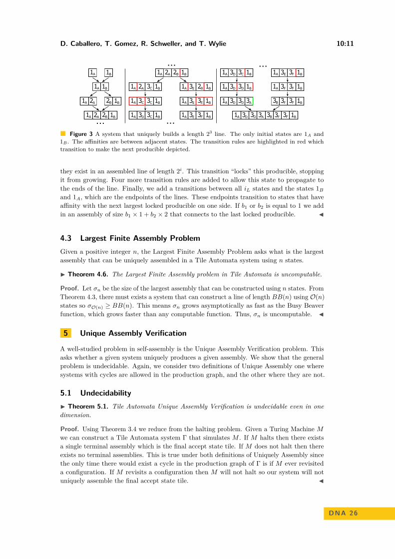
D. Caballero, T. Gomez, R. Schweller, and T. Wylie 10:11
1A 1B
1A 1B
1A 2A 2B 1B
1A 2A 3C 1B 1A 3E 2B 1B
1A 3C 3C 1B 1A 3E 3E 1B
1A 3D 3C 1B 1A 3E 3F 1B
1A 3D 3D 1B 1A 3F 3F 1B
1A 3D 3D 3A 3B 3F 3F 1B
1A 3D 3D 3A 3B 3F 3F 1B
1A 2A 2B 1B 1A 3D 3C 1B 1A 3E 3F 1B
1A 2A 2B 1B...
...
...
...
Figure 3 A system that uniquely builds a length 23 line. The only initial states are 1A and1B . The affinities are between adjacent states. The transition rules are highlighted in red whichtransition to make the next producible depicted.
they exist in an assembled line of length 2i. This transition “locks” this producible, stoppingit from growing. Four more transition rules are added to allow this state to propagate tothe ends of the line. Finally, we add a transitions between all iL states and the states 1Band 1A, which are the endpoints of the lines. These endpoints transition to states that haveaffinity with the next largest locked producible on one side. If b1 or b2 is equal to 1 we addin an assembly of size b1 × 1 + b2 × 2 that connects to the last locked producible. J
4.3 Largest Finite Assembly ProblemGiven a positive integer n, the Largest Finite Assembly Problem asks what is the largestassembly that can be uniquely assembled in a Tile Automata system using n states.
I Theorem 4.6. The Largest Finite Assembly problem in Tile Automata is uncomputable.
Proof. Let σn be the size of the largest assembly that can be constructed using n states. FromTheorem 4.3, there must exists a system that can construct a line of length BB(n) using O(n)states so σO(n) ≥ BB(n). This means σn grows asymptotically as fast as the Busy Beaverfunction, which grows faster than any computable function. Thus, σn is uncomputable. J
5 Unique Assembly Verification
A well-studied problem in self-assembly is the Unique Assembly Verification problem. Thisasks whether a given system uniquely produces a given assembly. We show that the generalproblem is undecidable. Again, we consider two definitions of Unique Assembly one wheresystems with cycles are allowed in the production graph, and the other where they are not.
5.1 UndecidabilityI Theorem 5.1. Tile Automata Unique Assembly Verification is undecidable even in onedimension.
Proof. Using Theorem 3.4 we reduce from the halting problem. Given a Turing Machine Mwe can construct a Tile Automata system Γ that simulates M . If M halts then there existsa single terminal assembly which is the final accept state tile. If M does not halt then thereexists no terminal assemblies. This is true under both definitions of Uniquely Assembly sincethe only time there would exist a cycle in the production graph of Γ is if M ever revisiteda configuration. If M revisits a configuration then M will not halt so our system will notuniquely assemble the final accept state tile. J
DNA 26
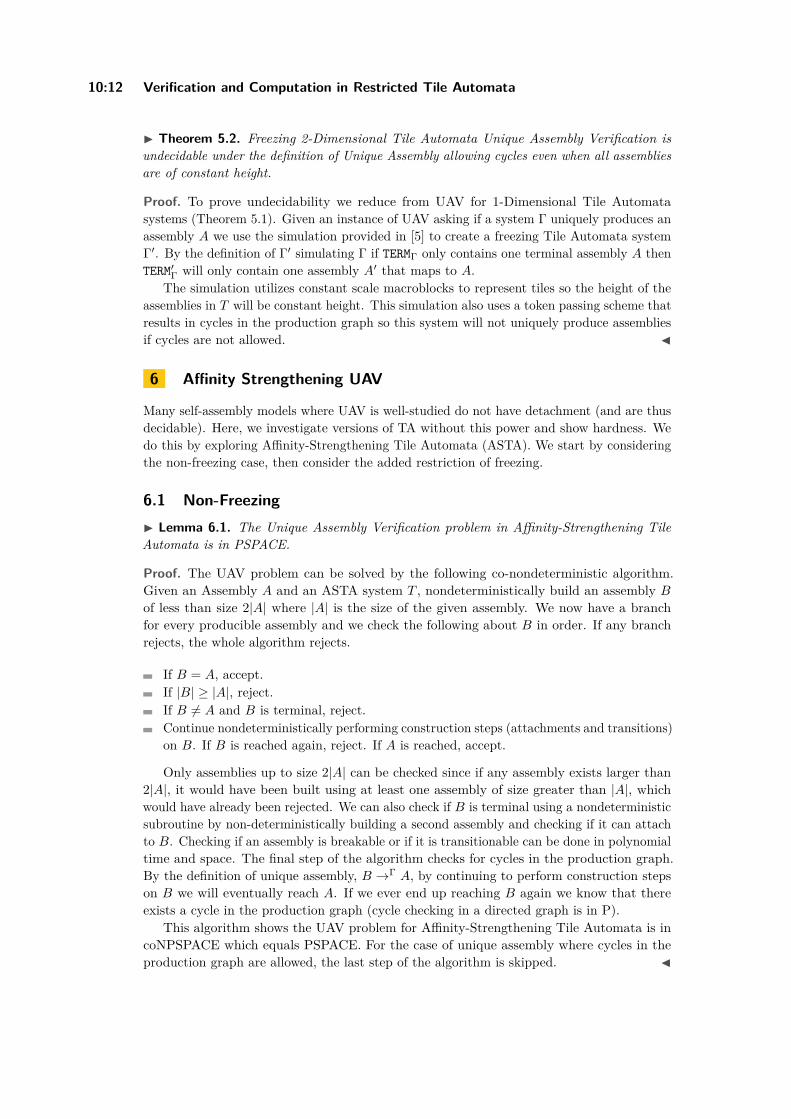
10:12 Verification and Computation in Restricted Tile Automata
I Theorem 5.2. Freezing 2-Dimensional Tile Automata Unique Assembly Verification isundecidable under the definition of Unique Assembly allowing cycles even when all assembliesare of constant height.
Proof. To prove undecidability we reduce from UAV for 1-Dimensional Tile Automatasystems (Theorem 5.1). Given an instance of UAV asking if a system Γ uniquely produces anassembly A we use the simulation provided in [5] to create a freezing Tile Automata systemΓ′. By the definition of Γ′ simulating Γ if TERMΓ only contains one terminal assembly A thenTERM′
Γ will only contain one assembly A′ that maps to A.The simulation utilizes constant scale macroblocks to represent tiles so the height of the
assemblies in T will be constant height. This simulation also uses a token passing scheme thatresults in cycles in the production graph so this system will not uniquely produce assembliesif cycles are not allowed. J
6 Affinity Strengthening UAV
Many self-assembly models where UAV is well-studied do not have detachment (and are thusdecidable). Here, we investigate versions of TA without this power and show hardness. Wedo this by exploring Affinity-Strengthening Tile Automata (ASTA). We start by consideringthe non-freezing case, then consider the added restriction of freezing.
6.1 Non-FreezingI Lemma 6.1. The Unique Assembly Verification problem in Affinity-Strengthening TileAutomata is in PSPACE.
Proof. The UAV problem can be solved by the following co-nondeterministic algorithm.Given an Assembly A and an ASTA system T , nondeterministically build an assembly Bof less than size 2|A| where |A| is the size of the given assembly. We now have a branchfor every producible assembly and we check the following about B in order. If any branchrejects, the whole algorithm rejects.
If B = A, accept.If |B| ≥ |A|, reject.If B 6= A and B is terminal, reject.Continue nondeterministically performing construction steps (attachments and transitions)on B. If B is reached again, reject. If A is reached, accept.
Only assemblies up to size 2|A| can be checked since if any assembly exists larger than2|A|, it would have been built using at least one assembly of size greater than |A|, whichwould have already been rejected. We can also check if B is terminal using a nondeterministicsubroutine by non-deterministically building a second assembly and checking if it can attachto B. Checking if an assembly is breakable or if it is transitionable can be done in polynomialtime and space. The final step of the algorithm checks for cycles in the production graph.By the definition of unique assembly, B →Γ A, by continuing to perform construction stepson B we will eventually reach A. If we ever end up reaching B again we know that thereexists a cycle in the production graph (cycle checking in a directed graph is in P).
This algorithm shows the UAV problem for Affinity-Strengthening Tile Automata is incoNPSPACE which equals PSPACE. For the case of unique assembly where cycles in theproduction graph are allowed, the last step of the algorithm is skipped. J
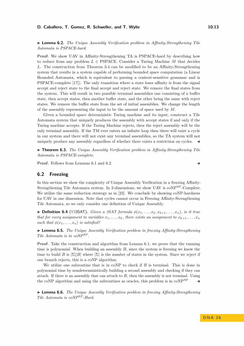
D. Caballero, T. Gomez, R. Schweller, and T. Wylie 10:13
I Lemma 6.2. The Unique Assembly Verification problem in Affinity-Strengthening TileAutomata is PSPACE-hard.
Proof. We show UAV in Affinity-Strengthening TA is PSPACE-hard by describing howto reduce from any problem L ∈ PSPACE. Consider a Turing Machine M that decidesL. The construction from Theorem 3.4 can be modified to be an Affinity-Strengtheningsystem that results in a system capable of performing bounded space computation (a LinearBounded Automata, which is equivalent to parsing a context-sensitive grammar and isPSPACE-complete [17]). The only transition where a state loses affinity is from the signalaccept and reject state to the final accept and reject state. We remove the final states fromthe system. This will result in two possible terminal assemblies one consisting of a bufferstate, then accept states, then another buffer state, and the other being the same with rejectstates. We remove the buffer state from the set of initial assemblies. We change the lengthof the assembly representing the input to be the amount of space used by M .
Given a bounded space deterministic Turing machine and its input, construct a TileAutomata system that uniquely produces the assembly with accept states if and only if theTuring machine accepts. If the Turing Machine rejects, then the reject assembly will be theonly terminal assembly. If the TM ever enters an infinite loop then there will exist a cyclein our system and there will not exist any terminal assemblies, so the TA system will notuniquely produce any assembly regardless of whether there exists a restriction on cycles. J
I Theorem 6.3. The Unique Assembly Verification problem in Affinity-Strengthening TileAutomata is PSPACE-complete.
Proof. Follows from Lemmas 6.1 and 6.2. J
6.2 FreezingIn this section we show the complexity of Unique Assembly Verification in a freezing Affinity-Strengthening Tile Automata system. In 2-dimensions, we show UAV is coNPNP-Complete.We utilize the same reduction strategy as in [23]. We conclude by showing coNP-hardnessfor UAV in one dimension. Note that cycles cannot occur in Freezing Affinity-StrengtheningTile Automata, so we only consider one definition of Unique Assembly.
I Definition 6.4 (∀∃3SAT). Given a 3SAT formula φ(x1, . . . , xk, xk+1, . . . , xn), is it truethat for every assignment to variables x1, . . . , xk, there exists an assignment to xk+1, . . . , xnsuch that φ(x1, . . . , xn) is satisfied?
I Lemma 6.5. The Unique Assembly Verification problem in freezing Affinity-StrengtheningTile Automata is in coNPNP.
Proof. Take the construction and algorithm from Lemma 6.1, we prove that the runningtime is polynomial. When building an assembly B, since the system is freezing we know thetime to build B is |Σ||B| where |Σ| is the number of states in the system. Since we reject ifone branch rejects, this is a coNP algorithm.
We utilize one subroutine that is in coNP to check if B is terminal. This is done inpolynomial time by nondeterministically building a second assembly and checking if they canattach. If there is an assembly that can attach to B, then the assembly is not terminal. Usingthe coNP algorithm and using the subroutines as oracles, this problem is in coNPNP J
I Lemma 6.6. The Unique Assembly Verification problem in freezing Affinity-StrengtheningTile Automata is coNPNP-Hard.
DNA 26

10:14 Verification and Computation in Restricted Tile Automata
C3
C2
C1
Variable 1 Variable 2 Variable 3 Variable 4
A0 0 0 0
1 1 1 1
0 0 0 0
1 1 1 1
0 0 0 0
1 1 1 1
0 0 0 0
1 1 1 1
(a)
C3C2C1A 1 1 1 1 0 0 0 0 0 0 0 0 1 1 1 1 C
(b)
Figure 4 Part of the construction for Theorem 6.6. (a) The base assemblies are constructednondeterministically. One is constructed for every possible variable assignment. (b) An example ofa base assembly fitting into a frame. Cx binds cooperatively to Cx−1 and the frame states.
Proof. Given an instance of ∀∃3-SAT, this reduction produces a τ = 2 freezing ASTA systemwhich uniquely assembles a target assembly if and only if the instance of ∀∃3-SAT is true.This system has stability threshold 2 to allow for cooperative binding in which two assembliesattach using affinities at two separate points, when one of the affinities alone would not bestrong enough for this attachment to be stable.
Overview. We first create an ‘L’-shaped base assembly contained in a larger frame (Figure4b) that encodes a variable assignment. Rows of this assembly represent clauses and columnsrepresent variables. Each clause is evaluated by cooperatively placing tiles that representthe assignment of the variable in its column, and whether the clause of its row is currentlysatisfied. Once the assignments are evaluated, additional tiles fill out the rest of the frame.If the assignment evaluates to false, then frame will be filled. If the assignment evaluates totrue, then there will be remaining spaces representing the assignment to the variables in thefirst quantifier. We construct a test assembly for every possible assignment to thee variablesthat can attach into that space. Once an assembly has completely filled out its frame, allstates inside transition into a target state and create our target assembly.
Base Assemblies. We construct a rectangular base assembly for every possible variableassignment to x1, . . . , xn, with the rows of this assembly representing clauses and columnsrepresenting variables. There are two sets of initial states for each variable: one for 0, and onefor 1. These sets of states attach to form length-4 line assemblies. The line assemblies haveaffinities with both the 0 and 1 line assemblies of the next variable. The nondeterministicnature of the model will ensure the creation of all possible combinations of these 0 and 1line assemblies (Figure 4a). Given m clauses in our 3SAT formula, the TA system includestiles with initial states C1, . . . , Cm. These states cooperatively attach to state A and a frame(Figure 4b). The frame ensures there is no unbounded growth. Tiles then cooperatively bindto fill out this structure. The affinities between these states and the variable line assembliesare encoded such that they evaluate if the variable assignment, represented by the baseassembly, satisfies the 3SAT formula (Figure 5a). The row containing Ci evaluates whetherthe ith clause is satisfied by the variable assignment of the base. U and S states cooperativelyattach to fill out a row- U indicating the clause has not yet been satisfied, and S indicatingthat it has. This is done by “passing” the assignment of the variable line upwards with aspecific encoding of the affinities. When an S state attaches, only S states can attach to itsright side. This allows a Y state to attach at the end of the row if a previous clause was notalready evaluated to be unsatisfied. If it is not satisfied, the rightmost state of that row willbe N , which does not allow a Y state to attach above it.

D. Caballero, T. Gomez, R. Schweller, and T. Wylie 10:15
SXy S
S S
SS
SU
U UUU
Xy0TX - 1
y
S
U1/0
S1/0
S Y
U N
YY
NN
NY
Affinity = 1
S1/0
1SXy
Xy
S0U
0SXy
Xy1U
0T
Xy1TX - 1
y1T
U
Y NA
B
States
0UXy
Xy1UC
0 1
UXy
0 1
SXy
0 1
TXy
0 1
(a)
0 0 0 0 1 1 1 1 0 0 0 01 1 1 1
C3C2C1 U U U 1
2 U U U13 S S S S S S S
CY
S S S S S S SS S S S S S S S YS S S S S S SS S S S S S S S Y
A0U11
11
110S
0S
1U 1U
E
(b)
0 0 0 0 1 1 1 1 0 0 0 01 1 1 1
C3C2C1 0U11 U U U
12 U U U
13 S S S S S S S
CY
11 Y
11 S S S S S S SS S S S S S S S N
A
0S
0U
1U 1S
F
U U U U U U U U U U U U U221U
231U
(c)
Figure 5 (a) Initial states needed to evaluate if the variable assignment satisfies the 3SAT formula.Choose 1 from A/B/C for each clause/variable combination. Choose A if 1 assigned to variable ysatisfies the xth clause, B if 0 satisfies, and C if the variable does not appear in that clause. T is aplaceholder for U or S, depending on which was chosen for each clause/variable combination. (b)Example of a 4-variable, 3-clause base assembly that is marked as true (top right “Y”). The assemblygrows downward, but interacts with the variable tile line to encode their variable assignment in theassembly’s geometry. (c) Example of a 4-variable 3-clause base assembly marked as false (top right“N”). The assembly grows to fill out the entire frame.
Once the rectangle is filled out an assembly will be marked as “True” or “False”, rep-resented by the top right Y /N state in the construction. (Figure 5b, 5c). True assembliesgrow downward, leaving a space between the base assembly and the frame. The shape of thisspace is an encoding of this assembly’s original variable assignment of x1, . . . , xk (Figure 5b).False assemblies also grow downward, but entirely fill out the frame of the base construction.
Test Assemblies. A set of test assemblies are also built using the same nondeterministicmethod used to create the base assemblies’ variable assignments. A test assembly is createdfor each assignment to variables x1, . . . , xk (Figure 6a). The geometry of a test assemblyencodes this variable assignment in a complementary fashion to that of a “True” base assemblyrepresenting the same assignment to x1, . . . , xk. This allows a test assembly to attach to a“True” base assembly with the same variable assignment to x1, . . . , xk, but not to any otherdue to that causing overlapping geometry. The test assemblies cooperatively bind with twostrength-1 affinities at two points (Figure 6b). A test assembly will only be terminal if thereis no base assembly matching its variable assignment that was marked as “True”.
Transition to Uniform Assembly. If the solution to the instance of ∀∃3SAT is true, allassemblies eventually grow/transition to one unique target assembly. To achieve this, thereare state transitions which allow every “True”/“False” flagged base assembly to grow into oneuniform assembly. For base assemblies marked “True”, to which a test assembly attached,the states needed to cooperatively bind these test assemblies to base assemblies having atransition rule to transition to state T . For assemblies marked “False”, a transition to stateT occurs when A and F (Figure 5c) are adjacent. Additional transition rules between stateT and all other states (excluding the frame states) allow this state to propagate throughoutthe entire assembly. The transitions used are shown in Figure 7a. These transitions willchange every state besides the frame states to state T . This is the target assembly for ourcreated instance of ASTA UAV (Figure 7b).
The only terminal assembly possibly produced that is not the target assembly is atest assembly representing a specific assignment to x1, . . . , xk that could not attach to anassignment assembly marked “True”, which represents the same variable assignment. Thus,the system only uniquely assembles the target assembly if the instance of ∀∃3SAT is true. J
I Theorem 6.7. The Unique Assembly Verification problem in freezing Affinity-StrengtheningTile Automata is coNPNP-Complete.
DNA 26
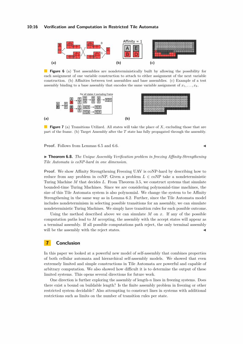
10:16 Verification and Computation in Restricted Tile Automata
B0
1D
(a)
Affinity = 1
DBA E
(b)
0 0 0 0 1 1 1 1 0 0 0 01 1 1 1
C3C2C1 U U U 1
2 U U U13 S S S S S S S
CY
S S S S S S SS S S S S S S S YS S S S S S SS S S S S S S S Y
A0U11
11
110S
0S
1U 1U
BDE
(c)
Figure 6 (a) Test assemblies are nondeterministically built by allowing the possibility foreach assignment of one variable construction to attach to either assignment of the next variableconstruction. (b) Affinities between test assemblies and base assemblies. (c) Example of a testassembly binding to a base assembly that encodes the same variable assignment of x1, . . . , xk.
TT
TX T
X
TX
T X
TT
T T
T T
T T
For all states X excluding Frame
TTD
BA
EAF
TT
(a)
TTTTTTT
TTTTTTT
TTTTTTT
TTTTTTT
TTTTTTT
TTTTTTT
TTTTTTT
TTTTTTT
TTTTTTT
TTTTT
TTTTT
TTTTT
TTTTT
TTTTT
TTTTT
TTTTT
TTTTT
TTTTT
TTTTT
(b)
Figure 7 (a) Transitions Utilized. All states will take the place of X, excluding those that arepart of the frame. (b) Target Assembly after the T state has fully propagated through the assembly.
Proof. Follows from Lemmas 6.5 and 6.6. J
I Theorem 6.8. The Unique Assembly Verification problem in freezing Affinity-StrengtheningTile Automata is coNP-hard in one dimension.
Proof. We show Affinity Strengthening Freezing UAV is coNP-hard by describing how toreduce from any problem in coNP. Given a problem L ∈ coNP take a nondeterministicTuring Machine M that decides L. From Theorem 3.5, we construct systems that simulatebounded-time Turing Machines. Since we are considering polynomial-time machines, thesize of this Tile Automata system is also polynomial. We change the system to be AffinityStrengthening in the same way as in Lemma 6.2. Further, since the Tile Automata modelincludes nondeterminism in selecting possible transitions for an assembly, we can simulatenondeterministic Turing Machines. We simply have transition rules for each possible outcome.
Using the method described above we can simulate M on x. If any of the possiblecomputation paths lead to M accepting, the assembly with the accept states will appear asa terminal assembly. If all possible computations path reject, the only terminal assemblywill be the assembly with the reject states. J
7 Conclusion
In this paper we looked at a powerful new model of self-assembly that combines propertiesof both cellular automata and hierarchical self-assembly models. We showed that evenextremely limited and simple constructions in Tile Automata are powerful and capable ofarbitrary computation. We also showed how difficult it is to determine the output of theselimited systems. This opens several directions for future work.
One direction is further exploring the assembly of length-n lines in freezing systems. Doesthere exist a bound on buildable length? Is the finite assembly problem in freezing or otherrestricted system decidable? Also attempting to construct lines in systems with additionalrestrictions such as limits on the number of transition rules per state.

D. Caballero, T. Gomez, R. Schweller, and T. Wylie 10:17
For the UAV problem, we show that the general case is undecidable. However, thecomplexity of the problem in freezing 1-dimensional systems is open. If the problem of askingwhether a system is bounded is decidable, then UAV is decidable by first identifying whethera system is bounded and then constructing the production graph and finding the terminalassemblies. The problem for freezing 2-dimensional systems with no cycles is also open.
Since Tile Automata can be seen as a generalization of 2HAM, our results can be comparedto the open problem of UAV in that model which is known to be in coNP. The most restrictedversion of Tile Automata we explore is Affinity Strengthening and freezing, which is only onelevel of the polynomial hierarchy above other generalizations of 2HAM such as allowing tilesto go into 3-dimensions or allowing a variable temperature. Further limiting Tile Automatamay provide more insight into the hardness of these problems.
References1 Leonard M. Adleman, Qi Cheng, Ashish Goel, Ming-Deh A. Huang, David Kempe, Pablo Mois-
set de Espanés, and Paul W. K. Rothemund. Combinatorial optimization problems inself-assembly. In Proceedings of the 34th Annual ACM Symposium on Theory of Computing,pages 23–32, 2002.
2 John Calvin Alumbaugh, Joshua J. Daymude, Erik D. Demaine, Matthew J. Patitz, andAndréa W. Richa. Simulation of programmable matter systems using active tile-based self-assembly. In Chris Thachuk and Yan Liu, editors, DNA Computing and Molecular Programming,pages 140–158, Cham, 2019. Springer International Publishing.
3 Sarah Cannon, Erik D. Demaine, Martin L. Demaine, Sarah Eisenstat, Matthew J. Patitz,Robert T. Schweller, Scott M Summers, and Andrew Winslow. Two Hands Are Better ThanOne (up to constant factors): Self-Assembly In The 2HAM vs. aTAM. In 30th InternationalSymposium on Theoretical Aspects of Computer Science (STACS 2013), volume 20 of LeibnizInternational Proceedings in Informatics (LIPIcs), pages 172–184. Schloss Dagstuhl–Leibniz-Zentrum fuer Informatik, 2013.
4 Angel A. Cantu, Austin Luchsinger, Robert Schweller, and Tim Wylie. Covert Computationin Self-Assembled Circuits. In 46th International Colloquium on Automata, Languages, andProgramming (ICALP 2019), volume 132 of Leibniz International Proceedings in Informatics(LIPIcs), pages 31:1–31:14, 2019.
5 Cameron Chalk, Austin Luchsinger, Eric Martinez, Robert Schweller, Andrew Winslow, andTim Wylie. Freezing simulates non-freezing tile automata. In International Conference onDNA Computing and Molecular Programming, pages 155–172. Springer, 2018.
6 Cameron Chalk, Austin Luchsinger, Robert Schweller, and Tim Wylie. Self-assembly of anyshape with constant tile types using high temperature. In Proc. of the 26th Annual EuropeanSymposium on Algorithms, ESA’18, 2018.
7 Matthew Cook. Universality in elementary cellular automata. Complex systems, 15(1):1–40,2004.
8 Joshua J. Daymude, Kristian Hinnenthal, Andréa W. Richa, and Christian Scheideler. Com-puting by programmable particles. In Distributed Computing by Mobile Entities: CurrentResearch in Moving and Computing, pages 615–681. Springer, Cham, 2019.
9 Erik D Demaine, Martin L Demaine, Sándor P Fekete, Mashhood Ishaque, Eynat Rafalin,Robert T Schweller, and Diane L Souvaine. Staged self-assembly: nanomanufacture of arbitraryshapes with o (1) glues. Natural Computing, 7(3):347–370, 2008.
10 Erik D. Demaine, Sarah Eisenstat, Mashhood Ishaque, and Andrew Winslow. One-dimensionalstaged self-assembly. In Proceedings of the 17th international conference on DNA computingand molecular programming, DNA’11, pages 100–114, 2011.
11 David Doty, Lila Kari, and Benoît Masson. Negative interactions in irreversible self-assembly.Algorithmica, 66(1):153–172, 2013.
DNA 26

10:18 Verification and Computation in Restricted Tile Automata
12 Constantine Evans. Crystals that Count! Physical Principles and Experimental Investigationsof DNA Tile Self-Assembly. PhD thesis, California Inst. of Tech., 2014.
13 Antonios G Kanaras, Zhenxin Wang, Andrew D Bates, Richard Cosstick, and Mathias Brust.Towards multistep nanostructure synthesis: Programmed enzymatic self-assembly of dna/goldsystems. Angewandte Chemie International Edition, 42(2):191–194, 2003.
14 Ryuji Kawano. Synthetic ion channels and dna logic gates as components of molecular robots.ChemPhysChem, 19(4):359–366, 2018. doi:10.1002/cphc.201700982.
15 Alexandra Keenan, Robert Schweller, Michael Sherman, and Xingsi Zhong. Fast arithmetic inalgorithmic self-assembly. Natural Computing, 15(1):115–128, March 2016.
16 Ceren Kimna and Oliver Lieleg. Engineering an orchestrated release avalanche from hydrogelsusing dna-nanotechnology. Journal of Controlled Release, April 2019. doi:10.1016/j.jconrel.2019.04.028.
17 Sige-Yuki Kuroda. Classes of languages and linear-bounded automata. Information andControl, 7(2):207–223, 1964. doi:10.1016/S0019-9958(64)90120-2.
18 Austin Luchsinger, Robert Schweller, and Tim Wylie. Self-assembly of shapes at constant scaleusing repulsive forces. Natural Computing, August 2018. doi:10.1007/s11047-018-9707-9.
19 Jennifer E. Padilla, Matthew J. Patitz, Raul Pena, Robert T. Schweller, Nadrian C. Seeman,Robert Sheline, Scott M. Summers, and Xingsi Zhong. Asynchronous signal passing for tileself-assembly: Fuel efficient computation and efficient assembly of shapes. In UnconventionalComputation and Natural Computation, pages 174–185. Springer, 2013.
20 Robert Schweller and Michael Sherman. Fuel efficient computation in passive self-assembly.In Proceedings of the 24th Annual ACM-SIAM Symposium on Discrete Algorithms, SODA’13,pages 1513–1525. SIAM, 2013.
21 Robert Schweller, Andrew Winslow, and Tim Wylie. Complexities for high-temperaturetwo-handed tile self-assembly. In Robert Brijder and Lulu Qian, editors, DNA Computing andMolecular Programming, pages 98–109, Cham, 2017. Springer International Publishing.
22 Robert Schweller, Andrew Winslow, and Tim Wylie. Nearly constant tile complexity for anyshape in two-handed tile assembly. Algorithmica, 81(8):3114–3135, 2019.
23 Robert Schweller, Andrew Winslow, and Tim Wylie. Verification in staged tile self-assembly.Natural Computing, 18(1):107–117, 2019.
24 Erik Winfree. Algorithmic Self-Assembly of DNA. PhD thesis, California Institute of Technology,June 1998.
25 Andrew Winslow. Staged self-assembly and polyomino context-free grammars. NaturalComputing, 14(2):293–302, 2015.
Turning MachinesIrina KostitsynaDepartment of Mathematics and Computer Science, TU Eindhoven, The Netherlandshttps://www.win.tue.nl/~ikostits/[email protected]
Cai WoodHamilton Institute and Department of Theoretical Physics, Maynooth University, Irelandhttps://[email protected]
Damien WoodsHamilton Institute and Department of Computer Science, Maynooth University, Irelandhttps://dna.hamilton.ie/woods/[email protected]
AbstractMolecular robotics is challenging, so it seems best to keep it simple. We consider an abstractmolecular robotics model based on simple folding instructions that execute asynchronously. TurningMachines are a simple 1D to 2D folding model, also easily generalisable to 2D to 3D folding. ATurning Machine starts out as a line of connected monomers in the discrete plane, each with anassociated turning number. A monomer turns relative to its neighbours, executing a unit-distancetranslation that drags other monomers along with it, and through collective motion the initial set ofmonomers eventually folds into a programmed shape. We fully characterise the ability of TurningMachines to execute line rotations, and to do so efficiently: computing an almost-full line rotationof 5π/3 radians is possible, yet a full 2π rotation is impossible. We show that such line-rotationsrepresent a fundamental primitive in the model, by using them to efficiently and asynchronouslyfold arbitrarily large zig-zag-rastered squares and y-monotone shapes.
2012 ACM Subject Classification Theory of computation → Models of computation
Keywords and phrases model of computation, molecular robotics, self-assembly, nubot, reconfigura-tion
Digital Object Identifier 10.4230/LIPIcs.DNA.2020.11
Funding Authors C. Wood and D. Woods are supported by European Research Council (ERC)award number 772766 and Science foundation Ireland (SFI) grant 18/ERCS/5746 (this manuscriptreflects only the authors’ view and the ERC is not responsible for any use that may be made of theinformation it contains).
Acknowledgements We thank Vera Sacristán and Suneeta Ramaswami for insightful ideas andimportant input. This work began at the 29th Bellairs Winter Workshop on ComputationalGeometry (March 21-28, 2014 in Holetown, Barbados), we thank Erik Demaine for organising awonderful workshop and providing valuable feedback, and the rest of the participants for providinga stimulating environment. We also thank Dave Doty and Nicolas Schabanel for helpful comments.
1 Introduction
The challenge of building molecular robots has many moving parts, as the saying goes.These include molecular parts that move relative to each other; units needing some sortof memory state; the ability to transition between states; and perhaps even the ability touse computation to drive robotic movements. Here we consider a simple robotic model ofreconfiguration called Turning Machines.
© Irina Kostitsyna, Cai Wood, and Damien Woods;licensed under Creative Commons License CC-BY
26th International Conference on DNA Computing and Molecular Programming (DNA 26).Editors: Cody Geary and Matthew J. Patitz; Article No. 11; pp. 11:1–11:21
Leibniz International Proceedings in InformaticsSchloss Dagstuhl – Leibniz-Zentrum für Informatik, Dagstuhl Publishing, Germany

11:2 Turning Machines
?
Figure 1 Turning Machine motivation: what shapes can be made by autonomously foldingstructures using simple local turning rules that effect non-local movement? Finding suitable abstractmodels and characterising their ability helps us to step back and create a vision of where we can go.
The main ethos behind our work is the notion of having a reconfigurable structure wherecomponent monomers actuate their position relative to their neighbours and governed bysimple actuation rules. Volume exclusion applies (two monomers can not occupy the sameposition in space), almost for free we get massive parallelism and asynchronicity, and thecomplexity of allowable state changes is small: start with a natural number and decrementstep-by-step to zero. The Turning Machine model embodies these concepts.
On the one hand, there are a number of senses in which molecular systems are bettersuited to robotic-style reconfiguration than macro-scale robotic systems: there is no gravitynor friction fighting against components’ actuation, and should we know how to exploitthem, randomness, freely diffusing fuel (robots need not carry all their fuel) and largenumbers of components are all readily available as resources. On the other hand, buildingnanoscale components presents a number of challenges including implementing computationalcontrollers at the nanoscale, as well as designing systems that self-assemble and interact in aregime where we can not easily send in human mechanics to diagnose and fix problems.
1.1 Turning machinesMonomers are the atomic components of a Turning machine and are arranged in a connectedchain on the triangular/hexagonal grid, with each monomer along the chain pointing at thenext. In an initial instance, the chain of monomers are sitting on the x-axis all pointingto the east. Each monomer has an initial integer turning number s ∈ Z, the monomer’sultimate goal is to set that number to 0: if s is positive, the monomer tries to simultaneouslydecrement s and turn anti/counter-clockwise1 by an angle of π/3, if s is negative, it triesto increment and turn clockwise by π/3.2 If s = 0 the monomer has reached its targetorientation and does not turn again. Figures 2 and 3 give the idea, and Section 2 gives a fulldefinition.
A key point is that although a monomer actuates by rotating the direction in which itpoints, when it does so it “drags” (translates) all monomers that come after it in the chainin the same way the rotation motion of an arm (around a shoulder) appears to translate aflag through the air, or the way a cam in an combustion engine converts rotational shaftmotion to translational piston motion.
1 We define counter-clockwise to be anticlockwise and use these terms interchangeably.2 Having the monomer turning angle be confined to the range (0, π/2] seems to capture a range of
interesting and important blocking behaviours that would otherwise be missed by the model. Havingthe angle be π/3, which leads us to the choice of triangular grid over the square grid, is a somewhatarbitrary choice in the model definition.

I. Kostitsyna, C. Wood, and D. Woods 11:3
1.2 Turning machines: the main programming challengeProgramming the model simply requires annotating an east-pointing line of monomers withturning numbers; an incredibly simple programming syntax.
Locally, individual monomers exhibit a small rotation, but globally this effects a largetranslation, or dragging, of many monomers. Thus globally, the main challenge is how toeffect global rotations – in other words how to use translation to simulate rotation. Inparticular, how to do this when lots of monomers are asynchronously moving and bumpinginto each other, potentially blocking each other from moving.
Blocking comes in two forms. Temporary blocking where one monomer is in the way ofanother, but eventually will get out of the way, and permanent blocking where all monomersblock each other in a locked configuration that will never free itself. We say that a targetstructure is foldable if all possible system trajectories lead to that structure, i.e. permanentblocking does not occur. A foldable structure may exhibit temporary blocking on sometrajectories, indeed most of the work for our positive results in this paper comes down toshowing that for certain folding tasks any blockings that happen are merely temporarykinks in the chain that are eventually worked out. We measure the amount of blocking byconsidering the completion time: a foldable structure where temporarily blocked monomerscan quickly become unblocked finishes faster than one where blocking takes a while tosort out. Our model of time assumes that the time to apply a turning rule to a givenunblocked monomer is an exponential random variable with rate 1, and the system evolves asa continuous time Markov chain with the discrete events being rules applied asynchronouslyand in parallel.
1.3 ResultsWe fully characterise the line rotation capability of the Turning Machine model, in twosenses. First, we show that for each of the angles θ ∈ π/3, 2π/3, π, 4π/3, 5π/3, and anynumber of monomers n ∈ N there is a Turning Machine with n monomers that starts on thex-axis and ends rotated by θ radians. We show this is the best one can do, that is, thatrotation of θ ≥ 2π is impossible (for any n > 7, there are always some trajectories thatare permanently blocked). Second, line rotation is fast. Up to constant factors the speedis optimal, completing in expected time O(logn). This shows that despite the fact thatline rotations in the range π ≤ θ ≤ 5π/3 experience large number of blockings along theirtrajectories, these blockings are all temporary, and do not conspire to slow the system downby more than a constant factor on average.
To illustrate that line rotation results are indeed a fundamental primitive in the model,as an application, we show how to fold any n × n square, rastered in a zig-zag fashion(Theorem 17). More generally, this allows us to fold any shape from a wide class calledy-monotone shapes (see Figure 9), all in optimal expected time O(logn).
1.4 Related and future workBesides finding insights at the interface of computation and geometry, another ultimate aimof this kind of work is bridge the gap between what we can imagine in theory and whatwe can engineer in the lab [19]. Biological systems actuated at the molecular scale provideinspiration: in the gastrulation phase of embryonic development of the model organismDrosophila melanogaster, large-scale rearrangements of the embryo are effected by thousandsof (nanoscale) molecular motors working together to rapidly push and pull the embryo into atarget shape [9, 17].
DNA 26
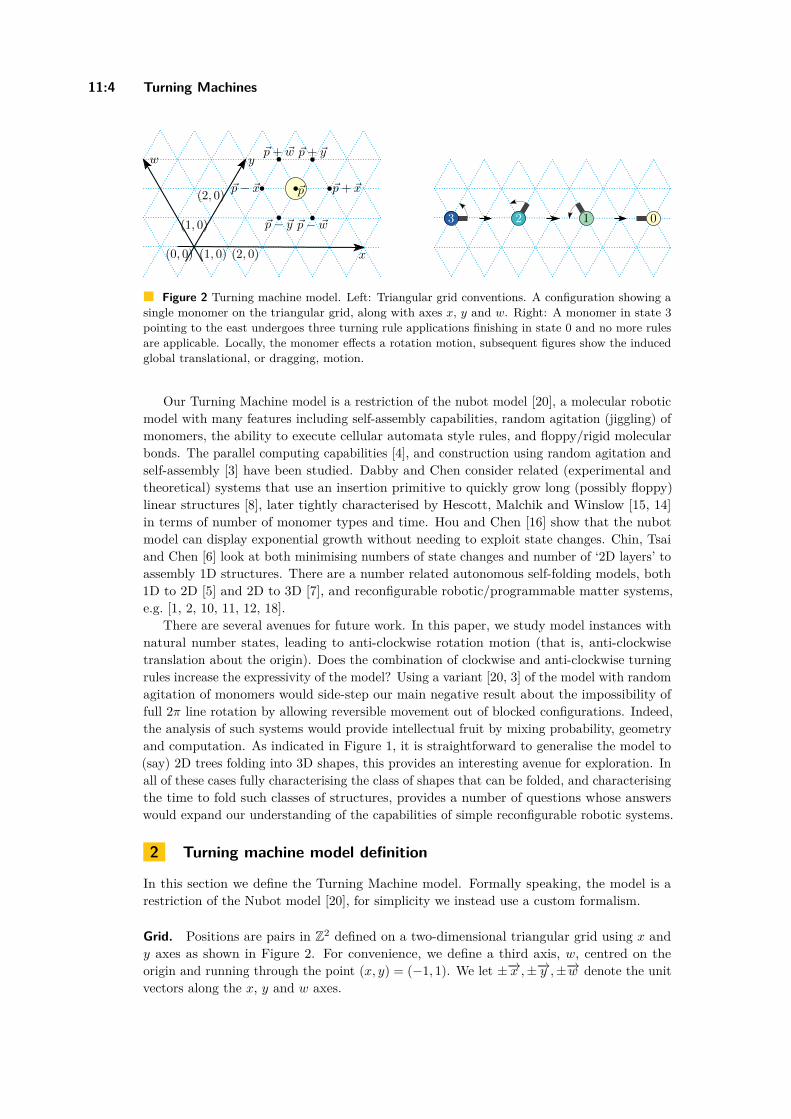
11:4 Turning Machines
(0, 0) (1, 0) (2, 0)
(1, 0)
(2, 0)~p+ ~x
~p− ~w
~p+ ~y
~p
~p− ~y
~p− ~x
~p+ ~w
x
yw
3 2 1 0
Figure 2 Turning machine model. Left: Triangular grid conventions. A configuration showing asingle monomer on the triangular grid, along with axes x, y and w. Right: A monomer in state 3pointing to the east undergoes three turning rule applications finishing in state 0 and no more rulesare applicable. Locally, the monomer effects a rotation motion, subsequent figures show the inducedglobal translational, or dragging, motion.
Our Turning Machine model is a restriction of the nubot model [20], a molecular roboticmodel with many features including self-assembly capabilities, random agitation (jiggling) ofmonomers, the ability to execute cellular automata style rules, and floppy/rigid molecularbonds. The parallel computing capabilities [4], and construction using random agitation andself-assembly [3] have been studied. Dabby and Chen consider related (experimental andtheoretical) systems that use an insertion primitive to quickly grow long (possibly floppy)linear structures [8], later tightly characterised by Hescott, Malchik and Winslow [15, 14]in terms of number of monomer types and time. Hou and Chen [16] show that the nubotmodel can display exponential growth without needing to exploit state changes. Chin, Tsaiand Chen [6] look at both minimising numbers of state changes and number of ‘2D layers’ toassembly 1D structures. There are a number related autonomous self-folding models, both1D to 2D [5] and 2D to 3D [7], and reconfigurable robotic/programmable matter systems,e.g. [1, 2, 10, 11, 12, 18].
There are several avenues for future work. In this paper, we study model instances withnatural number states, leading to anti-clockwise rotation motion (that is, anti-clockwisetranslation about the origin). Does the combination of clockwise and anti-clockwise turningrules increase the expressivity of the model? Using a variant [20, 3] of the model with randomagitation of monomers would side-step our main negative result about the impossibility offull 2π line rotation by allowing reversible movement out of blocked configurations. Indeed,the analysis of such systems would provide intellectual fruit by mixing probability, geometryand computation. As indicated in Figure 1, it is straightforward to generalise the model to(say) 2D trees folding into 3D shapes, this provides an interesting avenue for exploration. Inall of these cases fully characterising the class of shapes that can be folded, and characterisingthe time to fold such classes of structures, provides a number of questions whose answerswould expand our understanding of the capabilities of simple reconfigurable robotic systems.
2 Turning machine model definition
In this section we define the Turning Machine model. Formally speaking, the model is arestriction of the Nubot model [20], for simplicity we instead use a custom formalism.
Grid. Positions are pairs in Z2 defined on a two-dimensional triangular grid using x andy axes as shown in Figure 2. For convenience, we define a third axis, w, centred on theorigin and running through the point (x, y) = (−1, 1). We let ±−→x ,±−→y ,±−→w denote the unitvectors along the x, y and w axes.
I. Kostitsyna, C. Wood, and D. Woods 11:5
Monomer, configuration, trajectory. A monomer is a pair m = (s(m),pos(m)) wheres(m) ∈ Z is a state and pos(mi) ∈ Z2 is a position. A configuration, of length n ∈ N, is atuple of monomers c = (m0,m1, . . . ,mn−1) whose positions σ(c) = pos(m0),pos(m1), . . . ,pos(mn−1) define a length n− 1 simple directed path (or non-self-intersecting chain) in Z2
(on the triangular grid) and where pos(m0) = (0, 0).3A configuration is a tuple of n ∈ N monomers (m0,m1, . . . ,mn−1). A final configuration
has all monomers in state 0. A pair of configurations (ci, ci+1) is said to be a step ifci yields ci+1 via a single rule application (defined below) which we write as ci → ci+1.A trajectory, of length k, is a sequence of configurations c0, c1, . . . , ck−1 where, for eachi ∈ 0, 1, . . . , k − 2 the pair (ci, ci+1) is a step ci → ci+1. A Turning machine initialconfiguration c0 is said to compute the target configuration ct if all trajectories that start atc0 lead to ct, and is said to compute its target configuration if it reaches the configurationwith all monomers in state 0. A Turning machine instance is an initial configuration. For amonomer mi, we let s0(mi) denote its state in the initial configuration.
Turning rule: state decrement. Let Sinit ( Z be the set of states that appear in theinitial configuration.4 Let smin = min(Sinit ∪ 0) and smax = max(Sinit ∪ 0), and letS = smin, smin + 1, . . . , smax be the called the Turning machine state set. The turning rulesof a turning machine are defined by a function r such that for all states s ∈ (S \ 0):
r(s) =s− 1 if s > 0 ,s+ 1 if s < 0 .
(1)
Let C be the set of all configurations. The turning rule R : C × Z → C is a function andR(c, i) is said to be applicable to monomer mi in configuration c if s(mi) 6= 0 and the ruleis not blocked (defined below). If the rule is applicable, we write R(c, i) = c′ and say thatR(c, i) yields the new configuration c′, and we say that (c, c′) is a step.
Turning rule: blocking. For i ∈ 0, 1, . . . , n− 1, we define the head and tail of monomermi as head(mi) = mi+1,mi+2, . . . ,mn−1 and tail(mi) = m0,m1, . . . ,mi.
Consider the following tuple of unit vectors: ~d = (~x, ~y, ~w,−~x,−~y,−~w), and let ~dk denotethe kth element of that tuple. Let ~di = pos(mi+1)−pos(mi), i.e. the unit vector from monomermi to mi+1, and then let i′ = (i+2) mod 6. For a vector ~v ∈ Z2 we write mi+~v to mean themonomer mi translated by ~v. Define5 head→(mi) = mi+1 + ~di′ ,mi+2 + ~di′ , . . . ,mn−1 + ~di′ .If the set of positions of tail(mi) has a non-empty intersection with the set of positions ofhead→(mi) we say that the rule is blocked, and the rule is not applicable. If the rule is notblocked, it is applicable and the resulting next configuration is c′ = tail(mi), head→(mi) =m0,m1, . . . ,mi,mi+1 + ~di′ ,mi+2 + ~di′ , . . . ,mn−1 + ~di′ .
A configuration c is said to be permanently blocked if (a) not all states are 0, and (b)none of the monomers in c has an applicable rule. A monomer m within a configuration c issaid to be temporarily blocked if (a) m is not in state 0, and (b) there is no rule applicable tom, and (c) there is a trajectory starting at c that reaches a configuration c′ where there is arule applicable to m.
3 In the language of [20], one can imagine that for all i ∈ 0, 1, . . . , n− 2, there is a rigid bond betweenmonomer mi and monomer mi+1, and otherwise there are no bonds.
4 Throughout this paper, only natural number states are used. However, for generality, symmetry andpotential future work, we intentionally define the model to have integer states.
5 Another way to state this is that when a monomer mi moves, head(mi) translates in the directioncorresponding to the current direction of mi rotated by the angle 2π/3.
DNA 26

11:6 Turning Machines
= 1= 0
mi
`i
Figure 3 Left: The Turning Machine L1n that rotates a line of n = 11 monomers by π/3;
illustration for Lemma 5. Four configurations are shown. The initial configuration has all monomersin state 1 sitting on the x-axis, in the final configuration all are in state 0 and sitting on the π/3line. Two intermediate configurations are shown, respectively after 2, and then after 5, turning rulesapplications. Right: A configuration of some Turning Machine from the classM3
11 with the chainrunning from bottom left to top right. Lemmas 5 and 6 uses the fact that tail(mi) sits on or below`i, head(mi) sits on or above `i, and head→(mi) sits strictly above `i.
Time. A Turning Machine evolves as a continuous time Markov process. The rate for eachrule application is 1. If there are k applicable transitions for a configuration ci (i.e. k is thesum of the number of rule applications that can be applied to all monomers in ci), thenthe probability of any given transition being applied is 1/k, and the time until the nexttransition is applied is an exponential random variable with rate k (i.e. the expected timeis 1/k). The probability of a trajectory is then the product of the probabilities of each ofthe transitions along the trajectory, and the expected time of a trajectory is the sum of theexpected times of each transition in the trajectory. Thus,
∑t∈T Pr[t] · time(t) is the expected
time for the system to evolve from configuration ci to configuration cj , where T is the set ofall trajectories from ci to cj , and time(t) is the expected time for trajectory t.
I Example. The proof of Lemma 5 in Appendix A, and Figure 3, illustrate these concepts.
3 Classes of Turning Machines: line rotation and square
Every Turning Machine analysed in this paper starts with n ∈ N monomers, sitting on thex-axis, as formalised in the following definition.
I Definition 1 (M≤σn ). Let n, σ ∈ N. We let M≤σn denote the set of n-monomer TurningMachines with initial configuration c0 = m0,m1, . . . ,mn−1 having all monomers positionedon the x-axis (pos(mi) = (i, 0) ∈ Z2) and pointing to the east, and with initial states s0(mi)bounded by σ, i.e. s0(mi) ≤ σ for all 0 ≤ i ≤ n− 2, and s0(mn−1) = 0.
We next define a sub class ofM≤σn machines, called “line rotation” Turning Machines.
I Definition 2 (Line rotation Turning Machine). Let n ∈ N and let Lσn be the Turning Machinewith initial configuration of n monomers c0 = m0,m1, . . . ,mn−1 all pointing to the east,positioned on the x-axis (pos(mi) = (i, 0) ∈ Z2), and for 0 ≤ i ≤ n− 2 all monomers in thesame state s0(mi) = σ ∈ N+ and s0(mn−1) = 0.
I Remark 3. The initial monomer state σ ≥ 0 dictates that each monomer wishes to turn(have a rule applied) a total σ times, i.e. be rotated through an angle of σπ/3.

I. Kostitsyna, C. Wood, and D. Woods 11:7
αi
mi
mj
αi+1
αj
Figure 4 Illustration of turn angle (Definition 7). The turn angles αi and αi+1 are positive (andto the left), and αj is negative (and to the right).
I Remark 4 (Target configuration). For intuition, if there was no notion of blocking in theTurning Machine model, that is, if the model permitted self-intersecting configurations (whichit does not), then the final configuration c of the Turning Machine in Definition 2 is a straightline of monomers sitting along the ray that starts at the origin and is at an angle of σ π3 ,i.e. at positions (0, 0), (0,−1), . . . , (0,−(n− 1)) and all pointing to the west. We call c thedesired target configuration of the line rotation Turning Machine Lσn. Also, if there was nonotion of blocking: expected time to completion would be fast, O(logn) (by a generalisationof the analysis used in the proof of Lemma 5). However, a model with no blocking would berather uninteresting.
Figure 3 (left) illustrates Lemma 5 and Appendix A contains its straightforward, yetinstructive, proof.
I Lemma 5. For each n ∈ N, the line-rotating Turning Machine L1n computes its target
configuration, and does so in expected O(logn) time.
Lemma 6 is illustrated in Figure 3 (right).
I Lemma 6. Let n ∈ N and let L≤3n be a Turning Machine inM≤3
n (Definition 1). Let mi
for 0 ≤ i ≤ n− 1 be a monomer in some reachable configuration c of L≤3n . The monomers
head(mi) are positioned on or above `i, and tail(mi) are positioned on or below `i.
Proof. The claim follows from the fact that in any configuration of L≤3n , and for any
j ∈ 0, 1, . . . , n− 2 the angle of the vector−−−−−−−−−−−−−→pos(mj)pos(mj+1) (from monomer mj to mi+1)
is either 0, 60, 120, or 180 (and, in particular, is not strictly between 180 and 360). J
4 Tools for reasoning about Turning machines
The notion of turn angle of a monomer is crucial to our analysis and is illustrated in Figure 4.
I Definition 7 (Turn angle). Let c be the configuration of an n-monomer Turning Ma-chine and let 0 ≤ i < n − 1. The turn angle αi at monomer mi is the angle between−−−−−−−−−−−−−→pos(mi−1)pos(mi) and
−−−−−−−−−−−−−→pos(mi)pos(mi+1), and it is the positive counterclockwise angle if
the points pos(mi−1),pos(mi),pos(mi+1) make a left turn6, and the negative clockwise angleotherwise.
6 The notion of left or right turn along the three points pos(mi−1),pos(mi),pos(mi+1) can be formalisedby considering the line `i running through pos(mi), in the direction
−−−−−−−−−−−−−→pos(mi−1)pos(mi), noting that `i
cuts the plane in two, and defining the left- and right-hand side of the plane with respect to the vectoralong `i.
DNA 26
11:8 Turning Machines
For a monomer mi, the following definition gives a measure, ∆s(mi), of how its state s(mi)has progressed since the initial configuration.
I Definition 8. Let c be a reachable configuration of an n-monomer Turning Machine. Define∆s(mi) to be the number of rule applications to (moves of) the monomer mi from the initialconfiguration to c. That is, ∆s(mi) = s0(mi)− s(mi), where s0(mi) is the initial state ofmi, and s(mi) is the state of mi in configuration c.
I Lemma 9 (Difference of State is ≤ 2). Let n ∈ N, and let c be any reachable configurationof an n-monomer Turning Machine Tn with non-negative initial states, then
|∆s(mi)−∆s(mi+1)| ≤ 2 ,
for all 0 ≤ i < n− 1.
Proof. Let mtk, for t ∈ N and k ∈ 0, 1, . . . , n− 1, denote the kth monomer in the tth config-
uration ct. Initially, ∆s(m0j ) = 0 for all monomers mj , and thus |∆s(m0
i )−∆s(m0i+1)| = 0.
Observe, that |∆s(mi)−∆s(mi+1)| 6= 3 because otherwise pos(mi) = pos(mi+2) making ca self-intersecting (non-simple) configuration, contradicting its definition.
By Equation (1), when a rule is applied to one of mti or mt
i+1 its state decreases by 1and its ∆s(·) increases by 1. Then |∆s(mt
i) − ∆s(mti+1)| = |∆s(mt−1
i ) − ∆s(mt−1i+1)| ± 1.
When a rule is applied to some other monomer mk with i 6= k 6= j, then |∆s(mti) −
∆s(mti+1)| = |∆s(mt−1
i ) − ∆s(mt−1i+1)| ± 0. Thus, after each rule application the value of
|∆s(mi) −∆s(mi+1)| changes by at most 1, and as it cannot be equal to 3, we have that|∆s(mi)−∆s(mi+1)| ≤ 2. J
We can now show the following lemma, which proves a relation between the states of anytwo monomers of a Turning Machine and the geometry of the current configuration.
I Lemma 10. Let c be any reachable configuration of an n-monomer Turning Machine Tn,whose initial configuration c0 has all monomers pointing in the same direction, and let mi
and mj be two monomers of c such that i < j < n− 1, then
∆s(mj)−∆s(mi) = 3π
j∑k=i+1
αk ,
where αk is the turn angle at monomer mk.
Proof. For any intermediate configuration, the turn angle αi+1 between monomers mi andmi+1 depends only on the number of moves each monomer has made. Initially, αi+1 = 0,and it increases by π/3 each time monomer mi moves, and decreases by π/3 every timemonomer mi+1 moves. By Lemma 9, for two consecutive monomers mi and mi+1, in anyconfiguration, |∆s(mi)−∆s(mi+1)| ≤ 2. Hence, for a pair of consecutive monomers mi andmi+1, the turn angle αi+1 is in the range [−2π3 , 2
π3 ], and thus αi+1 = ∆s(mi+1)−∆s(mi).
Summing over all i gives the lemma conclusion. J
The following technical lemma is used extensively for our main results. Intuitively, it tellsus that high-state monomers are not blocked.
I Lemma 11. Let Tn ∈ Msn be a Turning Machine with maximum state s ≤ 5. In
any reachable configuration c of Tn no monomer mi with ∆s(mi) ≤ 1 is blocked (neithertemporarily blocked nor permanently blocked).

I. Kostitsyna, C. Wood, and D. Woods 11:9
βj
mk
mj
βk
mi
mi+1
βjmkmj
βk
mi
mi+1
Figure 5 Illustration for Lemma 11. Monomer mi is shown in black, head(mi) is shown in blueand tail(mi) is shown as the green curve plus the black monomer mi. Left: monomer mi is in itsinitial state (∆s(mi) = 0), and polygon P is traversed counter-clockwise. Right: monomer mi hasmoved once (∆s(mi) = 1), and polygon P is traversed clockwise.
Proof. Suppose, for the sake of contradiction, there is a blocked monomer mi with ∆s(mi) ≤1. Then there exist two monomers mj ∈ head(mi) and mk ∈ tail(mi) such that pos(mk) =pos′(mj), where pos′(mj) is the position of mj in head→(mi) (see Figure 5).
By definition of head and tail we know that k ≤ i < j. Consider the closed chainP = pos(mk),pos(mk+1), . . . ,pos(mj−1),pos(mj),pos(mk). Since configurations are simple,P defines a simple polygon. The turn angles of a simple polygon sum to 2π if the polygon istraversed anticlockwise (interior of P is on the left-hand side while traversing), or −2π if thepolygon is traversed clockwise (interior of P is on the right-hand side). For P , this sum isdefined as:
αP =j−1∑`=k+1
α` + βj + βk = ±2π ,
where α` is the turn angle at monomer m`, and βj and βk are the turn angles of the polygonat vertices pos(mj) and pos(mk) respectively (see Figure 5). More precisely,
α` = ∠(−−−−−→pos(m`)−
−−−−−−−→pos(m`−1),
−−−−−−−→pos(m`+1)−
−−−−−→pos(m`)) ,
βj = ∠(−−−−−→pos(mj)−
−−−−−−−→pos(mj−1),
−−−−−→pos(mk)−
−−−−−→pos(mj)) , and
βk = ∠(−−−−−→pos(mk)−
−−−−−→pos(mj),
−−−−−−−→pos(mk+1)−
−−−−−→pos(mk)) .
Furthermore, by Lemma 10,
∆s(mj−1)−∆s(mk) = 3π
j−1∑`=k+1
α` .
Thus,
∆s(mj−1) = ∆s(mk)+ 3π
j−1∑`=k+1
α` = ∆s(mk)+ 3π
(±2π−βj−βk) = ∆s(mk)±6− 3π
(βj+βk) .
Observe that when a monomer mi moves, its head translates in the direction correspondingto the current direction of mi rotated by angle 2π/3. Therefore, the state of mk can berepresented as a function of the state of mi and the angle βk, more precisely
∆s(mk) = ∆s(mi) + 2 + 3πβk .
DNA 26

11:10 Turning Machines
(See Figure 5 for an example.) Therefore, by the previous two equalities
∆s(mj−1) = ∆s(mi) + 2± 6− 3πβj .
Recall, that the angle βj ∈ [−2π/3, 2π/3], that 0 ≤ ∆s(mi) ≤ 1 by the assumption of thelemma, and that ∆s(mj−1) ≤ s. If the polygon defined by P is traversed counter-clockwise,then
∆s(mj−1) = ∆s(mi) + 8− 3πβj ≥ 0 + 8− 2 = 6 ,
which implies that s(mj−1) is out of the range of valid states, as mj−1 must have movedmore times as its initial state. Else, if the polygon P is traversed clockwise, then
∆s(mj−1) = ∆s(mi)− 4− 3πβj ≤ 1− 4 + 2 = −1 ,
which again implies that s(mj−1) is out of the range of valid states, as mj−1 must havemoved in the wrong direction. In either case we contradict that the state s(mj−1) is in therange of valid states, and, therefore, the monomer mi is not blocked. J
I Lemma 12. Let Lsn be a line-rotating Turning Machine with s ≤ 5. Let c be a reachableconfiguration of Lsn where each monomer mi in c has sc(mi) < s. Then the line-rotatingTurning Machine Ls−1
n has a reachable configuration c′ such that for every mi, sc′(mi) =sc(mi) and the geometry (chain of positions) of c is equal to that of the rotation of c′ by π/3around the origin.
Proof. Consider the sequence ρc rule applications (moves) that brings the initial configurationof Lsn to configuration c. We claim that ρc can be converted into another sequence ρc′ , ofthe same length, in which the first n− 1 moves are by monomers in state s.
First, we claim: for any two consecutive moves, where the second move is applied to amonomer in state s, swapping the two moves results in a valid sequence of moves transformingthe Turning Machine into the same configuration. Let the first move be applied to monomermi which transitions from state s′ to s′ − 1, and the second move be applied to monomer mj
which transitions from state s to s− 1. Suppose for the sake of contradiction that swappingthe moves results in at least one of the monomers mi or mj being blocked. We begin byattempting to apply the move to monomer mj , but, by Lemma 11, that move is not blocked.Then we attempt to apply a move to monomer mi, but that is not blocked either since thecoordinates of all monomers before and after swapping the two moves are exactly the same;i.e. the resulting configuration is a valid (non-self-intersecting) configuration in both cases.Hence neither monomer is blocked.
Thus, the original sequence of moves resulting in configuration c, can be converted intoanother sequence where the first n − 1 moves are applied to monomers in state s. Then,after the first n− 1 moves the configuration of Lsn is equivalent to the initial configuration ofLsn but rotated by π/3 and with all monomers in state s− 1. Hence equivalent to the initialconfiguration of Ls−1
n rotated by π/3.Applying the remaining moves to Ls−1
n will transform it into configuration c′. J
5 Line rotation to 5π/3
In this section we show that for 1 ≤ s ≤ 5 the line-rotation Turning Machine Lsn computesits target configuration of a sπ/3 rotated line (Theorem 13), and does so in expected timeO(logn) (Theorem 14). In addition to those results for any state s ≤ 5, in Appendix A we

I. Kostitsyna, C. Wood, and D. Woods 11:11
= 1
= 0
= 3
= 2
Figure 6 Example trajectory of the Turning Machine L3n that rotates a line of east-pointing
monomers by an angle of π. Illustration for Theorem 14 with s = 3 (and for Lemma 20 andTheorem 21 in Appendix A). Seven configurations are shown, the initial configuration has allmonomers in state 3 (blue), final in state 0 (yellow). Darker shading indicates later in time. A redbond (edge) indicates a blocked monomer. The proof of Lemma 20 shows that only monomers instate 1 are ever blocked and only when they are adjacent to a monomer in state 3, and that all suchblockings are temporary – if we wait long enough they become unblocked.
include stand-alone proofs for each of s = 1, s = 3, and s = 4 which showcase a variety ofgeometric techniques for analysing Turning Machine movement, but are not needed to proveour main results. Also, the cases of s = 1 and s = 3 are illustrated in Figures 3 and 6.
I Theorem 13. For each n ∈ N and 1 ≤ s ≤ 5, the line-rotation Turning Machine Lsncomputes its target configuration.
Proof. We prove by induction on 1 ≤ s ≤ 5 that any reachable configuration c of Lsn is notpermanently blocked.
Base case s = 1. In any configuration reachable by L1n, monomers have either state s = 1
or 0. Monomers in state s = 1 cannot be permanently blocked by Lemma 11. Thus, anynon-final configuration is not permanently blocked.
Assume for s− 1 the claim is true, i.e. it holds for Ls−1n . We will prove that for s it is
also true, i.e. it holds for Lsn. Suppose, for the sake of contradiction, there is a permanentlyblocked configuration c of Lsn for some n ∈ N and s ≤ 5. If there is no monomer in c in states, then by Lemma 12 there exists a corresponding configuration c′ in Ls−1
n with monomersm′0,m
′1, . . . ,m
′n−1, such that, for any monomer mi in c with state si < s the corresponding
monomer m′i in c′ has the same state si. Configurations c and c′ form chains equal up torotation by angle π/3. Configuration c′ is not blocked by the induction hypothesis, thusconfiguration c cannot be blocked either.
On the other hand, if there is a monomer mi in configuration c in state s, then byLemma 11 it is unblocked, and configuration c, again, is not blocked.
Hence the induction hypothesis holds for s, and Lsn does not have a reachable permanentlyblocked configuration. J
I Theorem 14. For each n ∈ N and 1 ≤ s ≤ 5, the line-rotation Turning Machine Lsncomputes its target configuration in expected O(logn) time.
Proof. By Theorem 13, Lsn computes its target configuration. For the time analysis we usea proof by induction on u ∈ 0, 1, . . . , s, in decreasing order.
The induction hypothesis is that for a reachable configuration cu of Lsn with maximumstate value u (there may be states < u in the configuration), the expected time to reach aconfiguration cu−1 with maximum state u− 1 is O(logn).
DNA 26

11:12 Turning Machines
For the base case we let u = s and assume c is such that all monomers are in state u.Hence c is an initial configuration and hence, by definition, is reachable. By Lemma 11,monomers in state s are never blocked and hence we claim that the first configuration withmaximum state u− 1 appears after expected time O(logn). To see this claim, note that foreach monomer mi in state s(mi) = u the rule application that sends mi to state u− 1 occursat rate 1, independently of the states and positions of the other monomers (by Lemma 11,there is no blocking of a monomer in state u = s). Since there are n monomers in state u,the expected time for all n to transition to u− 1 is [13]:
n∑k=1
1k
= O(logn) . (2)
We assume the inductive hypothesis is true for 0 < u+ 1 ≤ s, and we will prove it holdsfor u. Thus, there exists a reachable configuration cu where the maximum state value is u ≤ s,which is reachable from cu+1 in expected O(logn) time. Let there be n′ ≤ n monomers instate u in cu. By Lemma 12, there is a line-rotating Turning Machine Lun that has a reachableconfiguration c′u such that for every mi in cu, sc′
u(mi) = scu
(mi) and the positioning of cu isequal to the rotation of c′u by π/3 around the origin. By Lemma 11 monomers in state u inLun are never blocked, hence monomers in state u in cu are not blocked either. Setting n = n′
in Equation (2), and noting that O(logn′) = O(logn), proves the inductive hypothesis for u.Since we need to apply the inductive argument at most s ≤ 5 times, by linearity of
expectation, the expected finishing time for the s processes is their sum, 5 · O(logn) =O(logn). J
6 Line rotation to 2π is impossible
I Theorem 15. For all n ∈ N, n ≥ 7, the line-rotating Turning Machine L6n does not
compute its target configuration. In other words, there is a permanently blocked reachableconfiguration.
Proof. Figure 7, looking only at blue monomers and edges, shows a valid trajectory of L67 ,
then ends in a permanently blocked configuration, hence the lemma holds for n = 7.Let n > 7, and in Figure 7 let the red line segment denote a straight line `n−7 of n− 7
monomers co-linear with the red line segment. By inspection, it can be verified that (a) inall 25 configurations the line ` does not intersect any blue monomer, and moreover (b) thetransitions from configurations 1 through 14, configurations 17 through 23, and configuration24 to 25 are all valid, meaning that the length n− 7 line `n−7 does not block the transition.The transitions for configurations 14 through 17 are valid by Theorem 13 (with s = 3) andthe fact that the last blue monomer (the origin of `n−7) is strictly above all other bluemonomers (hence the 180 rotation of `n−7 proceeds without permanent blocking by bluemonomers). The transition for configuration 23 to 24 is valid by applying Lemma 5 (orTheorem 13, with s = 1) reflected through a horizontal line that runs through the last bluemonomer, and the fact that the last blue monomer (the origin of `n−7) is strictly below allother blue monomers (hence the 60 rotation of `n−7 proceeds without permanent blocking).Thus all transitions are valid and the permanently blocked configuration is reachable, givingthe lemma statement. J

I. Kostitsyna, C. Wood, and D. Woods 11:13
(1)
(2)
(3)
(4)
(5)
(6)
(7)
(8)
(9)
(10)
(11)
(12)
(13)
(14)
(15)
(16)
(19)
(20)
(21)
(22)
(23)
(24)
(25)
(17)
(18)
Figure 7 Impossibility of 360 line rotation, by showing that for all n ∈ N, the line-rotationTurning Machine L6
n has a reachable but permanently blocked configuration. Looking at the evolutionof the first seven monomers (i.e. ignore the rotation of the red line segment) we see one trajectory ofthe Turning machine that exhibits permanent blocking in the final (bottom-right) configuration,which has respective states 6,4,3,2,1,0,0. We imagine the red line segment as representing an arbitrarylong sequence of monomers running collinear with it, and transitions 14–16, 22–23, and 24–25, eachrepresenting the (many step) rotation of the red line by consecutive angles of 60. These rotations ofthe red line can proceed by two applications of Theorem 13 (first with s = 3, then with s = 1) andthe fact that the first monomer of the red line is strictly above, or below, the first seven monomers.Hence the final, permanently blocked, configuration is reachable no matter what length the redline is.
7 Folding zig-zag squares and y-monotone shapes
As a demonstration of our techniques, in this section we show how to build two shapes withTurning Machines: an n× n square, and any y-monotone shape.
We first define a specific curve which fills a square row by row in a zig-zag fashion. Anexample is shown in Figure 8 (left).
I Definition 16 (n× n zig-zag square). For any n ∈ N, an n× n zig-zag square is the lengthn2 configuration such that the position of monomer mi is given by the following expression:
pos(mi) =
(i%n, b inc) , if i%(2n) < n ,
(n− 1− i%n, b inc) , if i%(2n) ≥ n ,
where i%n denotes the remainder of i divided by n.
We now show that the zig-zag square can be built by a Turning Machine.
DNA 26
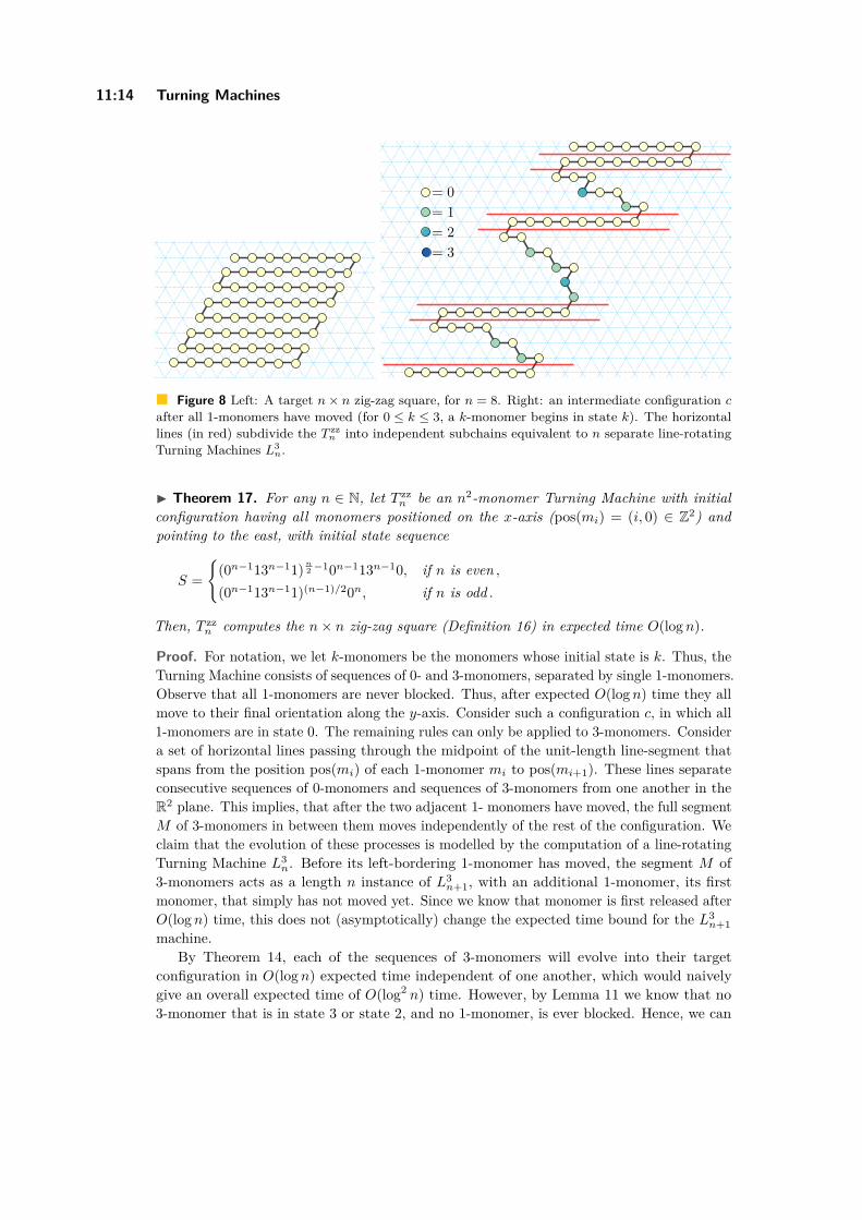
11:14 Turning Machines
= 1
= 0
= 3
= 2
Figure 8 Left: A target n× n zig-zag square, for n = 8. Right: an intermediate configuration cafter all 1-monomers have moved (for 0 ≤ k ≤ 3, a k-monomer begins in state k). The horizontallines (in red) subdivide the T zz
n into independent subchains equivalent to n separate line-rotatingTurning Machines L3
n.
I Theorem 17. For any n ∈ N, let T zzn be an n2-monomer Turning Machine with initial
configuration having all monomers positioned on the x-axis (pos(mi) = (i, 0) ∈ Z2) andpointing to the east, with initial state sequence
S =
(0n−113n−11) n2−10n−113n−10, if n is even ,
(0n−113n−11)(n−1)/20n, if n is odd .
Then, T zzn computes the n× n zig-zag square (Definition 16) in expected time O(logn).
Proof. For notation, we let k-monomers be the monomers whose initial state is k. Thus, theTurning Machine consists of sequences of 0- and 3-monomers, separated by single 1-monomers.Observe that all 1-monomers are never blocked. Thus, after expected O(logn) time they allmove to their final orientation along the y-axis. Consider such a configuration c, in which all1-monomers are in state 0. The remaining rules can only be applied to 3-monomers. Considera set of horizontal lines passing through the midpoint of the unit-length line-segment thatspans from the position pos(mi) of each 1-monomer mi to pos(mi+1). These lines separateconsecutive sequences of 0-monomers and sequences of 3-monomers from one another in theR2 plane. This implies, that after the two adjacent 1- monomers have moved, the full segmentM of 3-monomers in between them moves independently of the rest of the configuration. Weclaim that the evolution of these processes is modelled by the computation of a line-rotatingTurning Machine L3
n. Before its left-bordering 1-monomer has moved, the segment M of3-monomers acts as a length n instance of L3
n+1, with an additional 1-monomer, its firstmonomer, that simply has not moved yet. Since we know that monomer is first released afterO(logn) time, this does not (asymptotically) change the expected time bound for the L3
n+1machine.
By Theorem 14, each of the sequences of 3-monomers will evolve into their targetconfiguration in O(logn) expected time independent of one another, which would naivelygive an overall expected time of O(log2 n) time. However, by Lemma 11 we know that no3-monomer that is in state 3 or state 2, and no 1-monomer, is ever blocked. Hence, we can

I. Kostitsyna, C. Wood, and D. Woods 11:15
Figure 9 A y-monotone shape in R2 approximated with a zig-zag chain on the triangular grid.
analyse all n2 monomers as one system, noting that all such monomers complete in timeO(logn), at which point we have a reachable configuration that has all 3-monomers in eitherstate 0 and 1 (all others in state 0) which in turn finishes in O(logn) expected time.7 J
I Definition 18 (y-monotone shape). A set A ⊂ R2 is y-monotone, if any horizontal line hintersects S along one continuous segment of h.
Similarly to the construction of the zig-zag square presented above, we can build anapproximation of any y-monotone shape A by discretizing it and filling the resulting shaperow by row in a zig-zag manner (refer to Figure 9). The resulting state sequence of theTurning Machine T zz
n consists of intervals of 0-monomers and 3-monomers of various lengthsseparated by single 1-monomers.
We conclude with the following theorem statement. In it we assume that the statesequence S is such that the final configuration approximates some given y-monotone shape A.The proof is the same as that for Theorem 17 (but using a variety of horizontal segmentlengths n).
I Theorem 19. Let T y−monn be a Turning Machine with initial configuration having all
monomers positioned on the x-axis (pos(mi) = (i, 0) ∈ Z2) and pointing to the east, withinitial state sequence S consisting of intervals of 0- and 3-monomers separated by single1-monomers. Then T y−mon
n computes its target configuration in O(logn) expected time.
References1 Greg Aloupis, Sébastien Collette, Mirela Damian, Erik D Demaine, Robin Flatland, Stefan
Langerman, Joseph O’Rourke, Suneeta Ramaswami, Vera Sacristán, and Stefanie Wuhrer.Linear reconfiguration of cube-style modular robots. Computational Geometry, 42(6-7):652–663,2009.
2 Greg Aloupis, Sébastien Collette, Erik D. Demaine, Stefan Langerman, Vera Sacristán, andStefanie Wuhrer. Reconfiguration of cube-style modular robots using O(log n) parallel moves.In International Symposium on Algorithms and Computation, pages 342–353. Springer, 2008.
7 This is similar to the technique used in the proof of Theorem 14.
DNA 26

11:16 Turning Machines
3 Ho-Lin Chen, David Doty, Dhiraj Holden, Chris Thachuk, Damien Woods, and Chun-Tao Yang.Fast algorithmic self-assembly of simple shapes using random agitation. In DNA20: The 20thInternational Conference on DNA Computing and Molecular Programming, volume 8727 ofLNCS, pages 20–36, Kyoto, Japan, September 2014. Springer. Full version: arXiv:1409.4828.
4 Moya Chen, Doris Xin, and Damien Woods. Parallel computation using active self-assembly.Natural Computing, 14(2):225–250, 2014. arXiv version: arXiv:1405.0527.
5 Kenneth C. Cheung, Erik D. Demaine, Jonathan R. Bachrach, and Saul Griffith. Programmableassembly with universally foldable strings (moteins). IEEE Transactions on Robotics, 27(4):718–729, 2011.
6 Yen-Ru Chin, Jui-Ting Tsai, and Ho-Lin Chen. A minimal requirement for self-assembly oflines in polylogarithmic time. Natural Computing, 17(4):743–757, 2018.
7 Robert Connelly, Erik D. Demaine, Martin L. Demaine, Sándor P. Fekete, Stefan Langerman,Joseph S.B. Mitchell, Ares Ribó, and Günter Rote. Locked and unlocked chains of planarshapes. Discrete & Computational Geometry, 44(2):439–462, 2010.
8 Nadine Dabby and Ho-Lin Chen. Active self-assembly of simple units using an insertionprimitive. In SODA: The 24th Annual ACM-SIAM Symposium on Discrete Algorithms, pages1526–1536, January 2012.
9 Rachel E. Dawes-Hoang, Kush M. Parmar, Audrey E. Christiansen, Chris B. Phelps, Andrea H.Brand, and Eric F. Wieschaus. Folded gastrulation, cell shape change and the control ofmyosin localization. Development, 132(18):4165–4178, 2005.
10 Erik D. Demaine, Jacob Hendricks, Meagan Olsen, Matthew J. Patitz, Trent A. Rogers, NicolasSchabanel, Shinnosuke Seki, and Hadley Thomas. Know when to fold’em: self-assembly ofshapes by folding in oritatami. In DNA: International Conference on DNA Computing andMolecular Programming, pages 19–36. Springer, 2018.
11 Cody Geary, Pierre-Étienne Meunier, Nicolas Schabanel, and Shinnosuke Seki. Programmingbiomolecules that fold greedily during transcription. In MFCS: The 41st InternationalSymposium on Mathematical Foundations of Computer Science. Schloss Dagstuhl-Leibniz-Zentrum fuer Informatik, 2016.
12 Robert Gmyr, Kristian Hinnenthal, Irina Kostitsyna, Fabian Kuhn, Dorian Rudolph, ChristianScheideler, and Thim Strothmann. Forming tile shapes with simple robots. Natural Computing,pages 1–16, 2019.
13 Ronald L. Graham, Donald E. Knuth, and Oren Patashnik. Concrete mathematics, 1989.14 Benjamin Hescott, Caleb Malchik, and Andrew Winslow. Tight bounds for active self-assembly
using an insertion primitive. Algorithmica, 77:537–554, 2017.15 Benjamin Hescott, Caleb Malchik, and Andrew Winslow. Non-determinism reduces con-
struction time in active self-assembly using an insertion primitive. In COCOON: The 24thInternational Computing and Combinatorics Conference, pages 626–637. Springer, 2018.
16 Chun-Ying Hou and Ho-Lin Chen. An exponentially growing nubot system without statechanges. In International Conference on Unconventional Computation and Natural Computa-tion, pages 122–135. Springer, 2019.
17 Adam C Martin, Matthias Kaschube, and Eric F Wieschaus. Pulsed contractions of anactin–myosin network drive apical constriction. Nature, 457(7228):495–499, 2008.
18 Othon Michail, George Skretas, and Paul G. Spirakis. On the transformation capability offeasible mechanisms for programmable matter. Journal of Computer and System Sciences,102:18–39, 2019.
19 Hamid Ramezani and Hendrik Dietz. Building machines with DNA molecules. Nature ReviewsGenetics, pages 1–22, 2019.
20 Damien Woods, Ho-Lin Chen, Scott Goodfriend, Nadine Dabby, Erik Winfree, and Peng Yin.Active self-assembly of algorithmic shapes and patterns in polylogarithmic time. In ITCS:The 4th conference on Innovations in Theoretical Computer Science, pages 353–354. ACM,2013. Full version: arXiv:1301.2626 [cs.DS].

I. Kostitsyna, C. Wood, and D. Woods 11:17
A Line rotation by π/3, π and 4π/3
In this appendix we present proofs that line-rotating Turning Machine for respective anglesof π/3, π and 4π/3 terminates in expected time O(logn). These claims are superseded bythe results in the main paper, but we include the proofs as they give a number of techniquesto analyse the Turning Machine model.
A.1 Line rotation by π/3: L1n
The following proof of line rotation by π/3 radians is intended to be a simple exampleworked out in detail. Let L1
n be the Turning Machine defined in Definition 2 with σ = 1, asillustrated in Figure 3 (left).
I Lemma 5. For each n ∈ N, the line-rotating Turning Machine L1n computes its target
configuration, and does so in expected O(logn) time.
Proof. The initial configuration (Figure 3, left) of L1n is a line of n−1 monomers in state 1 with
an additional final monomer in state 0, i.e. at time 0 the n states are s(m0)s(m1) · · · s(mn−1) =1n−10. Since monomer states only change by decrementing from 1 to 0, any configuration onany trajectory of L1
n has its (composite) state of the form 0, 1n−10. Consider a configurationc in a trajectory of evolution of L1
n, and the corresponding state8 x ∈ 0, 1n−10. Let mci
denote the ith monomer of L1n in configuration c. For any i ∈ 0, 1, . . . , n − 2 such that
s(mci ) = 1, consider the unique configuration c′ where c → c′ and s(mc′
i ) = 0 (and, bydefinition of next configuration step, j 6= i implies s(mc′
j ) = s(mcj)).
We claim that tail(mci ) does not share any positions with head→(mc
i ), in other words,that c′ is a non-self-intersecting configuration. To show this, consider a horizontal line`i through monomer mc
i and observe that in c′ (and in c), the monomers tail(mci ) =
mc0,m
c1, . . . ,m
ci lie on or below `i (because the path pos(mc
0),pos(mc1), . . . ,pos(mc
i ) is con-nected and consists of unit length segments each at an angle of either 0 or 60 clock-wise relative to the x-axis), but the monomers head→(mc
i ) = mc′
i+1,mc′
i+2, . . . ,mc′
n−1 liestrictly above `i (because pos(mc′
i+1) is strictly higher than pos(mci ), and because the path
pos(m′i+1),pos(m′i+2), . . . ,pos(mc′
n−1) is connected and consists of unit length segments eachat an angle of 0 or 60 to the x-axis). Hence there are no blocked configurations reachableby L1
n (neither permanent nor temporary blocking).At each reachable configuration c, starting from the initial configuration, we can choose i
independently from the set of non-zero states. The expected time for the first rule applicationis 1/(n− 1) since it is the expected time of the minimum of n− 1 independent exponentialrandom variables each with rate 1. The next is 1/(n − 2), and so on. By linearity ofexpectation, the expected value of the total time T is E[T ] =
∑n−1k=1
1k = O(logn), where the
sum is the (n − 1)th partial sum of the harmonic series, known to have a O(logn) bound.Hence L1
n completes in expected O(logn) time. J
A.2 Line rotation by π: L3n
Next, we analyse line rotation of π radians.
I Lemma 20. Let L3n be a line-rotating Turning machine, then:
(i) any reachable configuration of L3n has no more than 2n/3 blocked monomers, and
(ii) there exists a configuration of L3n that has exactly 2n/3 blocked monomers.
8 In fact any x ∈ 0, 1n−10 is the state of a reachable configuration, but we don’t need to prove that.
DNA 26

11:18 Turning Machines
Proof. Consider any reachable configuration c of L3n, and let monomer mi be blocked in c.
By Lemma 11, monomers in state 2 and 3 are never blocked. By definition, monomers instate 0 are not blocked. Thus if mi is blocked it is in state 1, i.e. s(mi) = 1. We claim thatin this case either s(mi−1) = 3 or s(mi+1) = 3 (or both). Consider the following two casesfor s(mi+1):1. If s(mi+1) ∈ 1, 2, then by Lemma 6 all monomers of head→(mi), except its first monomer
m′i+1, lie strictly above `i, and since tail(mi) lies on or below `i, we get that tail(mi) doesnot intersect head→(mi), except possibly at pos(m′i+1). Whether pos(m′i+1) intersectstail(mi) depends on the state of mi−1:(a) If s(mi−1) ∈ 1, 2, then all monomers of tail(mi) lie strictly below `i (except its first
monomer mi which is not at position pos(m′i+1)), hence pos(m′i+1) cannot intersecttail(mi). Then mi cannot be blocked.
(b) If s(mi−1) = 0, then m′i+1 does not intersect tail(mi): Indeed, pos(mi−1) = pos(mi)+~x = pos(m′i+1) + 2~x 6= pos(m′i+1). Furthermore, let mj , mj+1, ..., mi−1 be thelongest consecutive subsequence of monomers in state 0 preceding monomer mi. Thenpos(mj), pos(mj+1), ..., pos(mi+1) are all strictly to the west of pos(mi). If j−1 ≥ 0,the non-zero-state9 monomer mj−1 enforces that the monomers m0, m1, ..., mj−1 liestrictly below `i. Thus mi is not blocked.
Therefore, monomer mi−1 can only be in state 3.2. If s(mi+1) = 0: Both head→(mi) and tail(mi) have monomers on `i, but we claim the
positions of head→(mi) do not intersect those of tail(mi). If s(mi−1) ∈ 1, 2, then allmonomers of tail(mi) exceptmi lie strictly below `i, and thus head→(mi) does not intersecttail(mi) (and recall that head→(mi) does not intersect pos(mi) because configurations aresimple). If s(mi−1) = 0 then the monomers M = mi−1,mi,m
′i+1 lie along `i (pointing
west). Note that a prefix of M is a suffix of tail(mi) and a (disjoint) suffix of M is aprefix of head→(mi). Hence, in order for tail(mi) to intersect head→(mi), one or bothmust depart from `i, but, by Lemma 6, tail(mi) can only do so by having monomersstrictly below `i, and head→(mi) can only do so by having monomers strictly above `i.Thus, monomer mi−1 can only be in state 3.
Therefore, if mi is blocked, then either mi−1 or mi+1 is in state 3, and thus is unblocked.Hence, there cannot be three monomers in a row which are blocked, resulting in Conclusion(i) of the lemma.
For Conclusion (ii), consider a line-rotating Turning Machine L3n with n = 3k for some k.
The configuration c with state sequence S = (131)k−1130 has exactly 2n/3 blocked monomers,as every monomer in state 1 is either blocked by a preceding monomer in state 3, or by afollowing monomer in state 3. J
I Theorem 21 (Rotate a line by π). For each n ∈ N, the line-rotating Turning Machine L3n
computes its target configuration, and does so in expected time O(logn).
Proof. By Lemma 20, no configuration has a permanently blocked monomer, hence everytrajectory of L3
n ends in the target configuration.At the initial step, the rate of rule applications is n − 1 (there are n − 1 monomers
in state 3). Over time, for successive configurations along a trajectory, the rate of ruleapplications may decrease for two reasons: (a) some monomers may be temporary blocked,and (b) after a monomer transitions to state 0 no more rules are applicable to it. We reasonabout both:
9 Which must be in state 1 or 2, since 3 would give a self-intersection along the configuration.
I. Kostitsyna, C. Wood, and D. Woods 11:19
(a) Lemma 20(ii) shows that a configuration with state sequence s = (131)n/3−1130 has2n/3 blocked monomers, and Lemma 20(i) states that no configuration has more than 2n/3blocked monomers for n divisible by 3. Using that fact, and in order to simplify the proof,we shall analyse a new, possibly slower, system where for any configuration c that has n′ ≤ nmonomers in state 6= 0, we “artificially” block 2n′/3 monomers.10 Since this assumptionmerely serves to slow the system, it is sufficient to give an upper bound on the expected timeto finish.
(b) A second “slowdown” assumption will be applied during the analysis and is justifiedas follows. Intuitively, the number of monomers transitioning to state 0 increases withtime, and since monomers in state 0 have no applicable rules, this causes a decrease inthe rate of rule applications. Consider a hypothetical continuous-time Markov system M ,with 3n steps with rate decreasing by 1 every third step, that is, with successive ratesn, n, n, n− 1, n− 1, n− 1, n− 2, . . . , 2, 1, 1, 1. By linearity of expectation, the expected valueof the finishing time T is the sum of the expected times E[ti] for each of the individual stepsi ∈ 1, 2, . . . , 3n:
E[T ] =3n∑i=1
E[ti] =n∑
m=13 · 1
m= 3
n∑m=1
1m
= 3Hn ≤ 3(ln(n) + 1) = O(logn) , (3)
where Hn is the nth partial sum of the harmonic series∑∞m=1
1m with Hn ≤ ln(n) + 1
(see [13]). Since, in L3n, it requires at least 3 steps to send a monomer from state 3 (the
initial state) to state 0, no trajectory sends monomers to state 0 at a faster rate than a(hypothetical) trajectory where a transition to state 0 appears at every third configuration(step). Hence, if there were no blocking whatsoever, then the expected time for L3
n would beno larger than 3Hn (given by Equation (3)).
Taking the blocking “slowdown assumption” in (a) into account, if the rate at step i is ri,then the slowed down rate is 1
3ri giving an expected time of
E[T ] =3n∑i=1
E[ti] =n∑
m=13 · 3
1 ·1m
= 9n∑
m=1
1m
= 9Hn ≤ 9(ln(n) + 1) = O(logn) . (4)
Since our two assumptions merely serve to define a new system that is necessarily slowerthan L3
n, we get the claimed expected time upper bound of O(logn) for L3n. J
A.3 Line rotation by 4π/3: L4n
I Lemma 22. Let mi be a blocked monomer in some reachable configuration c of a linerotation Turning Machine Lsn with n ∈ N and 1 ≤ s ≤ 4, and let mj ∈ head(mi) andmk ∈ tail(mi) be a pair of monomers which block the movement of mi, then in the subchainof Lsn from mk to mj−1 the number of unblocked monomers is at least half the number ofblocked monomers.
Proof. Similarly to the proof of Lemma 11, consider the closed chain P = pos(mk), ...,pos(mj), pos(mk). Let x(mi) denote the x-coordinate of the position of monomer mi, andy(mi) denote the y-coordinate of the position of monomer mi. Note, that for any `,
10The monomers are not necessarily geometrically blocked, we are merely stopping any rule from beingapplied to them. No configuration in a trajectory of L3
n witnesses a larger slowdown due to blockingthan the slowdown we have imposed on the configurations of T ′n.
DNA 26

11:20 Turning Machines
if s(m`) = s, then x(m`+1) = x(m`) + 1 and y(m`+1) = y(m`),if s(m`) = s− 1, then x(m`+1) = x(m`) and y(m`+1) = y(m`) + 1,if s(m`) = s− 2, then x(m`+1) = x(m`)− 1 and y(m`+1) = y(m`) + 1,if s(m`) = s− 3, then x(m`+1) = x(m`)− 1 and y(m`+1) = y(m`),if s(m`) = s− 4, then x(m`+1) = x(m`) and y(m`+1) = y(m`)− 1.
Let x(mk)− x(mj) = εx and y(mk)− y(mj) = εy, with εx, εy ∈ −1, 0, 1. The total changein x-coordinate and the total change in y-coordinate, when traversing P , is zero, that is,
j−1∑`=k
(x(`+ 1)− x(`)) + εx = 0 ,
j−1∑`=k
(y(`+ 1)− y(`)) + εy = 0 .
(5)
Considering the first part of Equation (5), and taking into account that the x-coordinateincreases only when traversing monomers in state s, and the x-coordinate decreases onlywhen traversing monomers in state s− 2 or s− 3, we get #(s) + εx = #(s− 2) + #(s− 3),where #(u) denotes the number of monomers with state u in the subchain from mk to mj−1.Observe, by Lemma 11, monomers in states s and s− 1 cannot be blocked, and since s ≤ 4,only the monomers in states s − 2 or s − 3 can be blocked. This implies, that within thesubchain from mk to mj−1, the number of blocked monomers is at most within an additivefactor 1 from the number of unblocked monomers.
Suppose, for a given subchain from mk to mj−1, the number of monomers in state sis strictly positive (that is, #(s) ≥ 1). Then, #(s) ≥ 1
2 (#(s − 2) + #(s − 3)), that is, inthe subchain, the number of unblocked monomers is at least half the number of blockedmonomers.
Now suppose that the number of monomers in state s in the subchain is zero (that is,#(s) = 0). As the blocked monomer mi has state either s − 2 or s − 3, the x-coordinatedecreases by 1 when traversing it. The x-coordinate only increases when traversing monomersin state s. Therefore, if there are no monomers in state s, εx has to be 1, and, besides theblocked monomer mi, the subchain from mk to mj−1 consists only of monomers in statess− 4 and s− 1.
Furthermore, as εx = 1, we have that pos(mk) = pos(mj) − ~w (that is, mi is in states − 3). We claim that there is at least one monomer in state s − 1 in the subchain frommk to mj−1. Indeed, consider the second part of Equation|5. Traversing the edge betweenmonomers mk and mj changes the y-coordinate by εy = y(mj) − y(mk) = y(−~w) = −1.Thus there has to be at least one monomer traversing which increases the y-coordinate. Thiscan only be a monomer in state s − 1. Thus, in the subchain from mk to mj−1, there isone blocked monomer mi and at least one unblocked monomer in state s− 1, and the totalnumber of unblocked monomers is at least the number of blocked monomers. J
I Theorem 23. For each n ∈ N and 1 ≤ s ≤ 4, the line rotation Turning Machine Lsncomputes its target configuration in O(logn) steps.
Proof. By Theorem 13 the Turning Machine Lsn computes its target configuration. Thatit computes the target configuration in O(logn) steps follows from the claim that in anyintermediate configuration c, the number of blocked monomers is not greater than 3n/4.
To prove this claim, consider a reachable configuration c of Lns , and consider all blockedmonomers B = mi : mi is blocked. Let ej,k be the edge connecting the positions of twomonomers mj and mk which block the movement of some monomer mi ∈ B (note, that mi
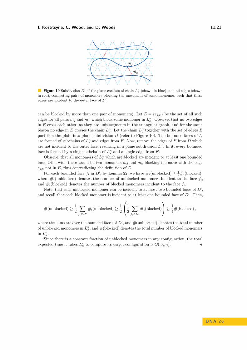
I. Kostitsyna, C. Wood, and D. Woods 11:21
mj
mk
Figure 10 Subdivision D′ of the plane consists of chain Lns (shown in blue), and all edges (shown
in red), connecting pairs of monomers blocking the movement of some monomer, such that theseedges are incident to the outer face of D′.
can be blocked by more than one pair of monomers). Let E = ej,k be the set of all suchedges for all pairs mj and mk which block some monomer in Lns . Observe, that no two edgesin E cross each other, as they are unit segments in the triangular graph, and for the samereason no edge in E crosses the chain Lns . Let the chain Lns together with the set of edges Epartition the plain into plane subdivision D (refer to Figure 10). The bounded faces of Dare formed of subchains of Lns and edges from E. Now, remove the edges of E from D whichare not incident to the outer face, resulting in a plane subdivision D′. In it, every boundedface is formed by a single subchain of Lns and a single edge from E.
Observe, that all monomers of Lns which are blocked are incident to at least one boundedface. Otherwise, there would be two monomers mj and mk blocking the move with the edgeej,k not in E, thus contradicting the definition of E.
For each bounded face fi in D′, by Lemma 22, we have #i(unblocked) ≥ 12 #i(blocked),
where #i(unblocked) denotes the number of unblocked monomers incident to the face fi,and #i(blocked) denotes the number of blocked monomers incident to the face fi.
Note, that each unblocked monomer can be incident to at most two bounded faces of D′,and recall that each blocked monomer is incident to at least one bounded face of D′. Then,
#(unblocked) ≥ 12
∑fi∈D′
#i(unblocked) ≥ 12
12
∑fi∈D′
#i(blocked)
≥ 14#(blocked) ,
where the sums are over the bounded faces of D′, and #(unblocked) denotes the total numberof unblocked monomers in Lns , and #(blocked) denotes the total number of blocked monomersin Lns .
Since there is a constant fraction of unblocked monomers in any configuration, the totalexpected time it takes Lsn to compute its target configuration is O(logn). J
DNA 26

Related Documents