Welcome message from author
This document is posted to help you gain knowledge. Please leave a comment to let me know what you think about it! Share it to your friends and learn new things together.
Transcript
International Hydrological Programme
Coastal Vulnerability and Freshwater Discharge
The Twenty-six IHP Training Course
27 November - 10 December, 2016
Nagoya, Japan
Institute for Space-Earth Environmental Research, Nagoya University
Supported by
International Hydrological Programme
Outline
A short training course “Coastal Vulnerability and Freshwater Discharge” will be
programmed for participants from Asia-Pacific regions as a part of the Japanese contribution to
the International Hydrological Program (IHP). The course is composed of a series of lectures
and practice sessions.
Objectives
Large number of population is living in coastal area of Asian countries. The area is
also important for various human activities including fisheries, transportation, farming, and
many other industries. The population explosion of the coastal area often makes pollution of
waters, both fresh and salt waters, inducing environmental problems in the area. Freshwater
input to the coastal area modified the circulation of waters. Large amount of materials are
known to be discharged to the coastal water with the freshwater as natural, and they played
important roles to keep the coastal ecosystem; however, the pollution of the freshwater also
alternate the coastal ecosystem. River is known as a major source of freshwater, and more
recently importance of underground discharge has been also recognized. Those freshwater
discharges are also changing significantly by the climate change, construction of dams on the
river, and use of freshwater. Coastal shallow area is often destructed to make a land for
farming, industry or living area with reclamation and other human activities. Recently, it was
shown that those coastal areas are vulnerable for tsunami caused by earthquake and storm surge
caused by typhoon, and radical changes can be happened by those natural hazards. It is
necessary to manage the area to make comfortable, productive and safe.
In this training course, the basic knowledge of physical, biological and chemical
environments of coastal waters, and forcing including freshwaters from river and underground
discharge, will be covered. Furthermore, interaction between nature of coastal area and human
will be discussed. Technical training on-board of Training Vessel Seisui-Maru, Mie University,
will cover the basic technics to sample waters, analyze the quality and interpret the data in large
estuarine Ise and Mikawa Bay. Demonstration of satellite and numerical models will be also
covered.
1
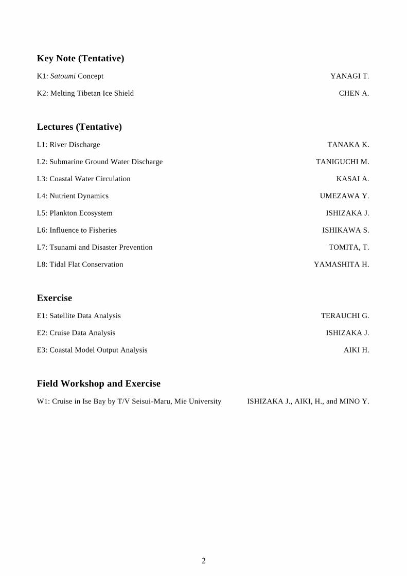
Key Note (Tentative)
K1: Satoumi Concept YANAGI T.
K2: Melting Tibetan Ice Shield CHEN A.
Lectures (Tentative)
L1: River Discharge TANAKA K.
L2: Submarine Ground Water Discharge TANIGUCHI M.
L3: Coastal Water Circulation KASAI A.
L4: Nutrient Dynamics UMEZAWA Y.
L5: Plankton Ecosystem ISHIZAKA J.
L6: Influence to Fisheries ISHIKAWA S.
L7: Tsunami and Disaster Prevention TOMITA, T.
L8: Tidal Flat Conservation YAMASHITA H.
Exercise
E1: Satellite Data Analysis TERAUCHI G.
E2: Cruise Data Analysis ISHIZAKA J.
E3: Coastal Model Output Analysis AIKI H.
Field Workshop and Exercise
W1: Cruise in Ise Bay by T/V Seisui-Maru, Mie University ISHIZAKA J., AIKI, H., and MINO Y.
2

Schedule (27 November to 10 December, 2016)
27 (Sunday) Arrival at Central Japan International Airport and Move to Nagoya University
28 (Monday) 09:30-09:40 Registration & Guidance
09:40-12:10 Lecture 1 by TANAKA K.
13:30-16:00 Lecture 2 by TANIGUCHI M.
17:00-19:00 Welcome Party
29 (Tuesday) 09:30-12:00 Lecture 3 by KASAI A.
14:00-16:30 Keynote 1 by YANAGI T.
30 (Wednesday) 09:30-12:00 Lecture 4 by UMEZAWA Y.
14:00-16:30 Keynote 2 by CHEN A.
(Move to Mie)
1 (Thursday) Cruise in Ise/Mikawa Bay
2 (Friday) Cruise in Ise/Mikawa Bay
3 (Saturday) Tour to Ise Shrine (Back to Nagoya)
4 (Sunday) Off
5 (Monday) 09:30-12:00 Lecture 5 by ISHIZAKA J.
13:30-17:00 Exercise 1 by TERAUCHI G.
6 (Tuesday) 09:30-12:00 Lecture 6 by ISHIKAWA S.
13:30-16:00 Exercise 2 by ISHIZAKA J.
7 (Wednesday) 09:30-12:00 Lecture 7 by TOMITA, T.
13:30-17:00 Exercise 3 by AIKI H.
8 (Thursday) 09:30-12:00 Lecture 8 by YAMASHITA H.
13:30-17:00 Making reports and discussions
9 (Friday) 09:30-11:30 Report presentations and discussions
11:30-12:00 Completion ceremony of this course
13:30-15:30 Farewell party
10 (Saturday) Departure from Central Japan International Airport
3

4
K1: Concept and Practices of Satoumi in Japan and Lessons Learned Tetsuo Yanagi (International EMECS Center, Kobe) Abstract
The coastal seas in the world suffer from environmental problems such as eutrophication, natural disaster, fish resources decreasing, environmental degradation and so on. In order to solve such complicated problems, successful Integrated Coastal Management (ICM) is necessary. Method of ICM in Japanese SATOUMI (the coastal sea with high biodiversity and productivity under the human interaction such as the Seto Inland Sea, Shizukawa Bay and the Sea of Japan) is introduced in this lecture.
ICM is an increasingly important topic for the public, scientist, policy makers and NPO related to environmental problems in the coastal sea. ICM is also a very rapidly evolving field. Dissemination of ICM in Satoumi where high biodiversity and productivity are realized under the human interaction is very useful for the people interested in the environmental problems in the coastal seas of the world.
A new concept “Satoumi” was firstly proposed by Prof.T.Yanagi in 1998 and the first book “Sato-Umi” was published in 2006 and the second book “Japanese Commons in the Coastal Seas: How the Satoumi Concept Harmonizes Human Activity in Coastal Seas with High Productivity and Diversity” was published in 2010 with Springer.
This lecture will present the most advanced results on ICM in Satoumi. This lecture would target graduate students and advanced college students as well as stakeholders (such as policy makers and environmental organizations), oceanographers and economists.
5

6
2016/9/29
1
Concept and Practices of Satoumi in Japan and
Lessons Learned
International EMECS CenterProfessor Emeritus of Kyushu University
Tetsuo YANAGI
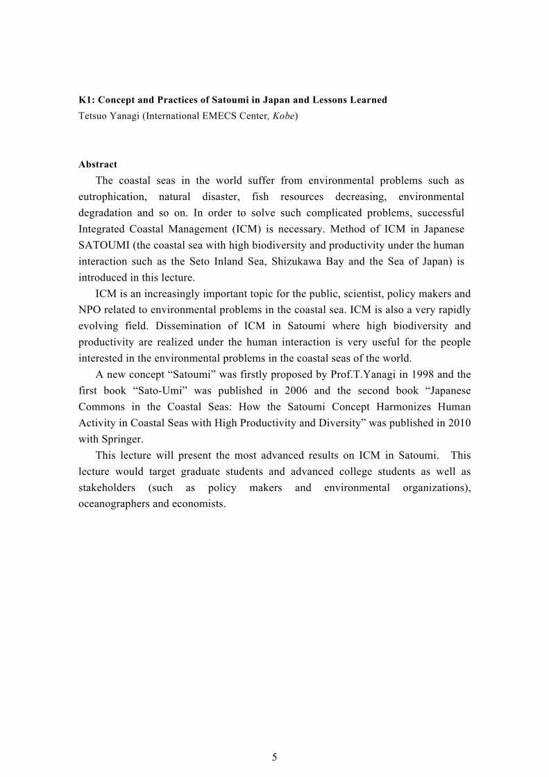
Satoyama and Satoumi
Satoyama : Forest with high productivity and bio-diversity under the human interaction
Satoumi : Coastal sea with high productivity and bio-diversity under the human interaction
Yanagi (1998, 2006)
2001
Satoyama ‐ Satoumi
VillageCity
Satoyama
High Mountain
Satoumi
Deep Sea
Eco‐tone
Eco‐tone
Shallow sea
Sea grass bedTidal flats
Claim of some ecologists
• Human interaction in Satoyama may increase bio‐diversity,
• but human interaction in coastal sea may decrease bio‐diversity
7
2016/9/29
2
Bio‐diversity and Human interactionHigh bio‐diversity =
Many kinds of habitat (nursery ground, feeding place, spawning ground) and
no‐climax (climax=simple habitat)
1) Human interaction to arrange habitat – High biodiversity
2) Human interaction to stop the transfer to climax of flora –
High biodiversity
Yanagi (2009) Human interaction and bio‐diversity. Ocenography in Japan, 18, 393‐398 (in Japanese)
Example of increasing bio‐diversity under the human interaction
Tidal stone weir (Nagaki, Kachi in Okinawa)
Tawa ed. (2007)Siraho Conservation Organization HP
High water
Low water
Nagaki at Shiraho, Ishigaki Island, Okinawa
Reconstructed by local people of Shiraho Village in 2006
Data of Kamimura
Species number
Spr. Aut. Spr. Aut. Spr. Aut. Spr. Aut. Spr
2006 AutumnReconstruction Kamimura (2011)
Many fish at the spot without eel grass
Fish roads
Fisheries in the eel grass bed
Suitable scale, formation and arrangement of eel grass bed
Few fish in the central part of eel grass bed
Seeds of eel grass
Many fish at the rim of eel grass bed
Tanimoto(2009)
Spot harvest in eel grass bed resulted in increasing bio-diversity
Tanimoto (2012)
Mitsukuchi Bay
8
2016/9/29
3
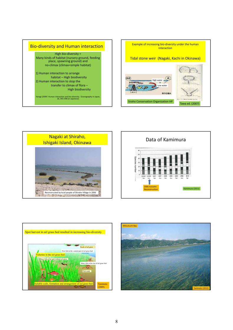
Field experiment of fish catch inside and outside of eel grass bed in Mitsukuchi Bay
2009/8/26~27
Outside (rim):Stas. 1、2、5inside:Stas. 3、4
inside outside
2009/8/4 Mitukuchi Bay (217ha)
132.75 132.755 132.76 132.765 132.77 132.775 132.78 132.78534.255
34.26
34.265
34.27
34.275
34.28
34.285
132.75 132.755 132.76 132.765 132.77 132.775 132.78 132.78534.255
34.26
34.265
34.27
34.275
34.28
34.285
0 to 2 2 to 4 4 to 6 6 to 8 8 to 10 10 to 12 12 to 141
234
5
132.75 132.755 132.76 132.765 132.77 132.775 132.78 132.78534.255
34.26
34.265
34.27
34.275
34.28
34.285
2009/8/27 Mitukuchi Bay
132.757 132.758 132.759 132.76 132.761 132.762 132.763 132.764 132.765 132.766 132.76734.26
34.261
34.262
34.263
34.264
34.265
34.266
34.267
132.757 132.758 132.759 132.76 132.761 132.762 132.763 132.764 132.765 132.766 132.76734.26
34.261
34.262
34.263
34.264
34.265
34.266
34.267
1
2
3
4
5
132.757 132.758 132.759 132.76 132.761 132.762 132.763 132.764 132.765 132.766 132.76734.26
34.261
34.262
34.263
34.264
34.265
34.266
34.267
0 100 200 300 400 500
Tanimoto (2009)
Mitsukuchi Bay
Gill net
2009年8月27日
0
5
10
15
20
25
30
35
1 2 3 4 5
測点
個体数
アマモ場内
0
2
4
6
8
10
12
1 2 3 4 5測点
種類数
アマモ場内
魚種 数量 魚種 数量 魚種 数量 魚種 数量 魚種 数量ギザミ 1 ギザミ 1 メバル 1 オコゼ 1 メバル 1メバル 3 メバル 4 フグ 2 フグ 2 コノシロ 8コノシロ 1 コノシロ 1 コノシロ 3 コチ 2アイナメ 1 コチ 1 ネコサメ 2 サバ 1タイ 1 タイ 1 ハゼ 1 キス 2ハゼ 1 ハゼ 3 イシガニ 3 コイワシ 1エソ 1 オコゼ 1 イシガニ 13イシガニ 5 タナゴ 1 シャコ 1ウニ 2 イシガニ 2 ニシ 1ニシ 1 ナマコ 1 ヒトデ 1
51 2 3 4
Tanimoto (2009)
insideinside
outside
outside
individual
species
Biodiversity and human interaction
high
low
biodiversity
Stop transfer to climax
Seagrass cutting
Tidal stone weir
Habitat creationhigh
Too much interaction
No interaction Too much interaction No interaction
Hinase Fishermen’s Union, Okayama
Sta.22
Decrease of eel grass bedsDecrease of fish catch
Fishermen in HinaseFishermen’s Unionbegan the eel grass bed creationin 1985and continued until now
Due to agricultural chemicaland increase of turbidity
1940s 1960 1985
eel grass bed in 2011
more than 200ha
Recovery to 1/3 of eel grass bed in 1940s
Fish catch by set net
9
2016/9/29
4
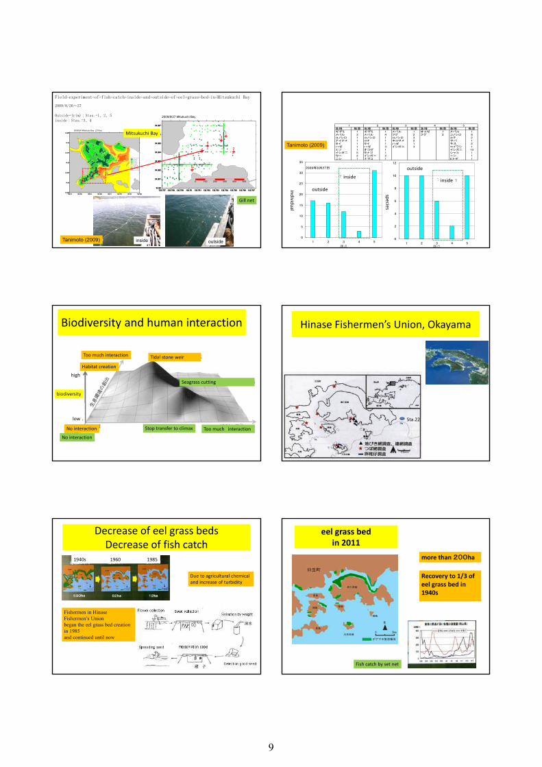
カキ養殖
カキ養殖区画漁業権
幼稚仔
保育場
200 400 1000m8006000
<凡例>
;Oyster culture ground
;eel grass bed
;artificial reef
;誘導滞留礁
;成魚生息場
;消波施設
a
b
c
d
e
b
b
b
b
ba
a
a
a
a
a
a
a
a
c
d
d
d
d
鹿久居島
頭島
大多府島
鶴島
アマモ場再生区域
区画漁業権
a
f
f
e
Oyster culture groundsOyster culture was began in 1963 → expanded in 1980s→ Okayama Oyster brand in 1996
Fish stock enhancement
Oyster culture and eel grass bedwin‐win relation
• Decrease of water temperature in eel grass bed(due to leaves of eel grass)
→ decrease of mortality of oyster
• Attached diatom and small animal on the leaves of eel grass→ increase of growth rate of oyster
・ Decrease of wave height by oyster raft → decrease of eel‐grass root damage
・ Grazing of phytoplankton and detritus → Increase of transparency →Increase of eel‐grass beds area
Recovery of sea bed litter andDirect selling of harvest
Fishery of Hinase Fishermen’s Union• Marine environment conservation: eel grass
bed creation, recovery of sea bed litters、Sea bed cultivation
• Resources management:Release of juvenile、Days of prohibition of fishing
• Added values:Direct selling of harvest、Oyster baking restaurant, information from direct selling →Adjustment of fishing activity
Necessity of dissemination of fishermen’s activities:Consumer may pay extra money for the marine environment conservation
Fishery and Marine Ecosystem Conservation
• Fishery is said to be the worst environment destroying activity
• It may result in conservation of marine ecosystem to harvest all levels biota in marine food chain
Galcia et al. (2012) Reconsidering the consequences of selective fisheries. Science, 335, 1045‐1047
・ Hinase set net= Selective fishing
• Cooking of all kinds of fish from small to large →Dissemination of Hinase culture – fishing and cooking
Agreement for Hinase Fisheries
May 2012
1) Fishermen’s Union2) Okayama Prefecture3) Okayama COOP4) Research Institute for Satoumi
Creation
10
2016/9/29
5
Committee for management
C
Committee for ICM
ManagementRule makingMonitoringPenalty
Local government
Okayama Pref.Bizen City
Chamber of Commerce
Local IndustryLocal people
UniversityNPOProfessional
Hinase Fishermen Union
Local Fishermen
Terra Scientific Publishing Company2007
Sato-Umi-A new concept for coastal sea
management-1.Introduction2.Mankind and coastal sea
2.1 Richness of the coastal sea2.2 Crisis of the coastal sea
3. Mankind and the forest3.1 Sato-Yama
4. Sato-Umi4.1 Concept of Sato-Umi4.2 Harvest of sea-glass bed4.3 New technology4.4 Stock enhancement and fish
culture4.5 Sea farming4.6 Fish resources management
5. Environmental ethics5.1 Environmental ethics and
Commons5.2 Preservation and Conservation5.3 Environmental education
6. Concluding remarks
Satoumi: Japanese Commons in the Coastal Sea
published in 2012 from Springer
12 examples of satoumi creation by Japanesefishermen and international activities on Satoumi creation are introduced
28
Jakarta Bay
Seribu Island
Northern CoastKarawang
Java Sea
Brackish water Pond
Java Sea
Sato Umi Session-EMECS9 Conference –Baltimore-28/8-2011
Aquaculture pond
30
Consulting Activities in 2008
Sato Umi Session-EMECS9 Conference –Baltimore-28/8-2011
11
2016/9/29
6
Integrated Multi Trophic Aquaculture
coast
Mangrove
Tilapia Sea cucumber
Shrimp Sea grass
Bivalve Sea weed
Mangrove
Zero emission aquaculture 32
ZONATION MODEL OF THE DIVERSITY PRODUCT of GAPURA AND ENVIRONMENTAL SITUATION
Coastal Environment
Irrigation/Channel
Channel
Pond
Java Sea
Mangrove Plant
Pond
Tilapia
Shrimp
Gracilaria
Green Muscle
Zonation Model
Experiment Jun.‐Sep., 2010
Rice Field
Tilapia/Cat FishShrimp‐Sea Weed
Milk Fish
Sea
Sato Umi Session-EMECS9 Conference –Baltimore-28/8-2011
33
EXPERIMENTAL DESIGNINTEGRATED MULTI-TROPIC AQUACULTURE (IMTA)
Bio-recycling-System
PrototypeIMTA
P-4P-3
P-2P-1
P-2
P-4
P-1 : Shrimp PondP-2 : Shrimp and Tilapia PondP-3 : Shrimp ,Tilapia and
Seaweed Pond P-4 : Shrimp ,Tilapia , Seaweed
and Green Muscle Pond
± 500 m2
Sato Umi Session-EMECS9 Conference –Baltimore-28/8-201134
PHYSICAL‐CHEMICAL Water Quality Profile of the Treated Breackish water Pond
Treatment
Temp (o C)
Salinity(ppt) pH
DO (mg/l)
Turb.(NTU)
TSS(mg/l
)
BOD5(mg/l
)
P‐1 30.81 24.94 7.92 6.02 121.83 36.5 1.66P‐2 30.77 23.11 7.87 6.16 127.46 22.33 0.71P‐3 30.92 22.48 7.90 6.43 157.08 22.83 0.24
P-4 30.94 22.91 7.91 6.47 177.67 18 1.18
Physical
Treatment DIN (ppm)
DIP (ppm)
Sulfide (ppm)
Iron (ppm)
P1.3 1.081 0.33 0.03 0.12P2.3 2.154 0.21 0.03 0.21P3.3 2.086 0.74 0.03 0.53P4.3 1.207 0.15 0.02 0.39
Chemical
0.000
0.500
1.000
1.500
2.000
2.500
P1.3 P2.3 P3.3 P4.3
DIN (ppm) DIP (ppm) Sulfide (ppm) Iron (ppm)
Sato Umi Session-EMECS9 Conference –Baltimore-28/8-2011
35
Treatment
Black Tiger Shrimp
Tilapia Sea Weed Green Muscle Total Biomass Weight Gain
T‐0 T‐3 T‐0 T‐3 T‐0 T‐3 T‐0 T‐3 TotalT‐0
TotalT‐3
Biomass
(gr) (gr) (gr) (gr) (gr) (gr) (gr) (gr) (gr) (gr) (gr)P‐1 0.1 21.7 0.1 21.7 21.6P‐2 0.1 8.0 18.7 187.6 18.8 195.6 176.8P‐3 0.1 8.1 27.4 238.7 43.1 70.7 246.8 176.1P-4 0.1 34.2 29.4 159.0 44.4 2048.0 66.6 57.7 140.6 2298.8 2158.3
22 177 176
2158
0
2000
4000
P-1 P-2 P-3 P-4
Weight Gain Biomass (gr)
Suhendar, Yanagi and Ratu (2014) Coastal Marine Science, 37 36
Expansion of Dissemination Program
3. Anambas1. Karawang
1.
3.2.
4.5.
2. Kampar 4. Bantaeng 5. Tual
Sato Umi activities in Indonesia from 2011Success of IMTA (Integrated Multi-Trophic level Aquaculture) in Karawan
12
2016/9/29
7
Satoumi‐GAPRA International Workshop at Jakarta, Indonesia on 13‐14 March, 2013
Establishment of Fisheries Management System based on Satoumi Concept in the Pan‐Pacific Region (2012‐2016)
• 0.12 million US dollars/year sponcered by JFA
• Western, central and eastern parts in the North‐Pacific
• Manual, Workshops, Data‐base• Under the umbrella of PICES(Pacific ICES;
International Council for the Exploration of the Sea)
2012.3 2012.3United Nation University
International Workshopon Satoumi
• 1st Workshop in 2008 at Shanghai• 2nd Workshop in 2009 at Manila• 3rd Workshop in 2010 at Kanazawa• 4th Workshop in 2011 at Baltimore• 5th Workshop in 2012 at Hawaii• 6th Workshop in 2013 at Marmaris (Turky)• 7th Workshop in 2014 at Tokyo• 8th Workshop in 2015 at Da Nang (Vietnam)• 9th Workshop in 2016 at Saint Petersberg (Russia)• 10th Workshop in 2017 at Bordeaux (France)
Difference of human‐nature relation between Japan and Western Countries
Japan with high population density cannot have preserved zone
over-usewise-use
under-use
13
2016/9/29
8
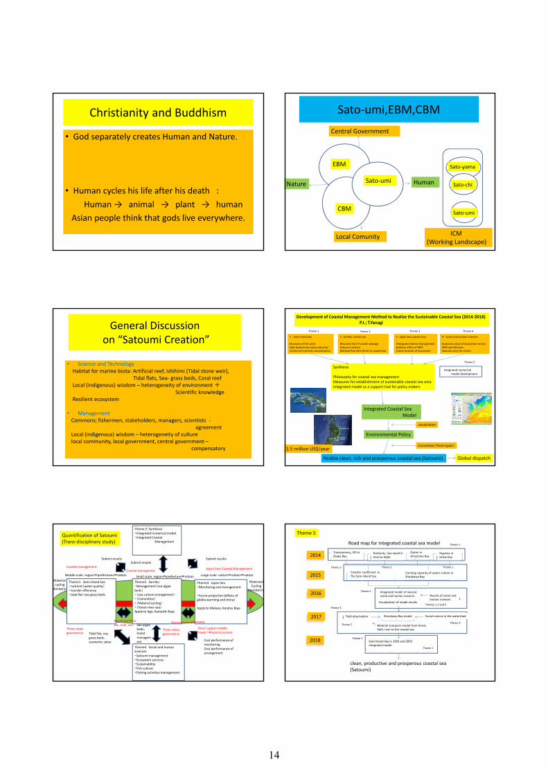
Christianity and Buddhism
• God separately creates Human and Nature.
• Human cycles his life after his death : Human → animal → plant → human
Asian people think that gods live everywhere.
Sato‐umi,EBM,CBMCentral Government
Local Comunity
HumanNature Sato‐umi
CBM
EBM
Sato‐umi
Sato‐chi
Sato‐yama
ICM(Working Landscape)
General Discussionon “Satoumi Creation”
• Science and TechnologyHabitat for marine biota: Artificial reef, Ishihimi (Tidal stone weir),
Tidal flats, Sea‐ grass beds, Coral reefLocal (indigenous) wisdom – heterogeneity of environment +
Scientific knowledgeResilient ecosystem
• ManagementCommons; fishermen, stakeholders, managers, scientists ‐
agreementLocal (indigenous) wisdom – heterogeneity of culturelocal community, local government, central government –
compensatory
Synthesis
Philosophy for coastal sea managementMeasures for establishment of sustainable coastal sea areaIntegrated model as a support tool for policy makers
Development of Coastal Management Method to Realize the Sustainable Coastal Sea (2014‐2018)P.I.; T.Yanagi
1.Seto Inland Sea
Decrease of fish catchHigh biodiversity and productionControl of nutrients concentration
2.Sanriku coastal sea
Recovery from Tsunami‐damageSatoumi creationMaterial flux from forest to coastal sea
3.Japan Sea coastal area
Intergovernmental managementSpillover effect of MPAFuture forecast of ecosystem
4.Social and Human sciences
Economic value of ecosystem serviceMPA and fisheriesSatoumi story for citizen
Integrated Coastal Sea Model
Realize clean, rich and prosperous coastal sea (Satoumi)
Environmental Policy
Committee(Three types)
visualization
Theme 1 Theme 2 Theme 3 Theme 4
Integrated numericalmodel development
Theme 5
Global dispatch
1.5 million US$/year
Theme4 Social and human sciences・Satoumi management・Ecosystem services・Sustainability・Fish culture・Fishing activities management
Theme 5: Synthesis・Integrated numerical model・Integrated Coastal
Management
Theme2 Sanriku・Management(sea‐algae beds)・(sea culture arrangement)・(Committee)・(Material cycling)・(forest‐river‐sea)Apply to Ago, Kamaishi Bays
Submit resultsSubmit results
Material cycling
Monitoring
Sea algae beds、forest management
Tidal flat, sea‐grass beds, economic value
Three‐steps governence
Three‐steps governence
Theme1 Seto Inland Sea・nutrient(water quality)・transfer efficiency・tidal flat・sea‐grass beds
Theme3 Japan Sea・Monitoring and management
・future projection (effetcs of globla warming and china)
Apply to Wakasa, Karatsu Bays
Coastal managementCoastal managemet
Cost performance of monitoringCost performance of arrangement
Middle scale:region⇔prefectures⇔nation Small scale:region⇔prefecture⇔nation Large scale:nation⇔nation⇔nation
Aquaculture raft⇔MPABay/Nada⇔Forest, river, sea
River(upper‐middle‐lower)⇔ocenic current
Submit results
MateraialCycling
Monotoring
Quantification of Satoumi(Trans‐disciplinary study)
Japan Sea・Coastal Management
大阪湾透明度・DO 播磨灘栄養塩・ノリ 広島湾カキ 洞海湾貧酸素26年度
27年度
28年度
29年度
30年度
瀬戸内海転送効率モデル 山田湾最適養殖モデル
自然・社会統合モデル
“見える化”
社会・人文科学の
研究成果
志津川湾モデル
“森-里-川-海物質輸送モデル”
現地の観測結果 流域の社会科学情報
1950年と2050年の瀬戸内海モデル
人の暮らしのあり方
“自然科学、社会・人文科学統合モデル”
「きれいで、豊かで、賑わいのある持続可能な沿岸海域」
の実現のための行政施策に反映
統合的沿岸海域モデル実施のフロー Theme 1
Theme 1 Theme 2Theme 5
Theme 4
Theme 4Theme 2
Theme 5
Theme 5
Theme 5
Themes 1,2 and 3
志津川
2014
2015
2016
2017
2018
Transparency, DO in Osaka Bay
Nutrients, Sea‐weed inHarima‐Nada
Oyster in Hiroshima Bay
Hypoxia in Dokai Bay
Transfer coefficient in The Seto Inland Sea
Carrying capacity of oyster culture in Shizukawa Bay
Integrated model of natural,social and human sciences Results of social and
human sciencesVisualization of model results
Shizukawa Bay modelField observation Social science in the watershed
Material transport model from forest, field, river to the coastal sea
Seto Inland Sea in 1950 and 2050 Integrated model
clean, productive and prosperous coastal sea (Satoumi)
Road map for integrated coastal sea model
Theme 1
Theme 5
14
2016/9/29
9
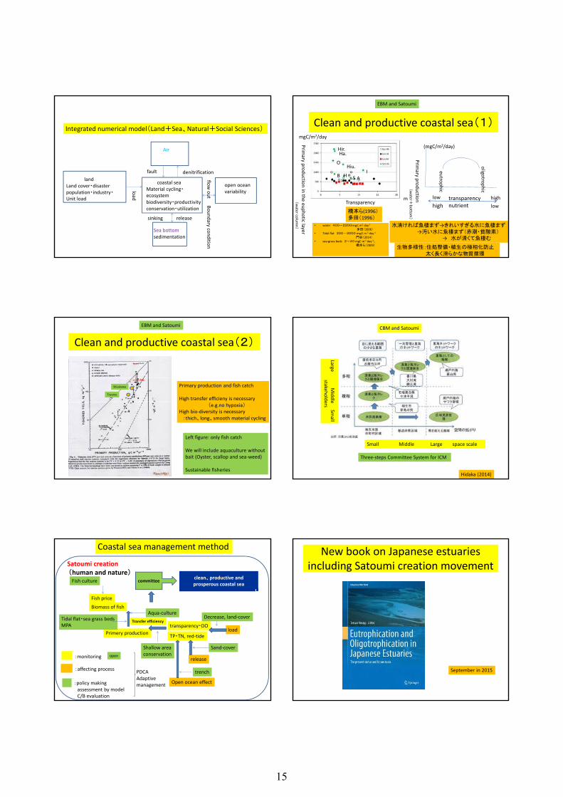
coastal seaMaterial cycling・ecosystembiodiversity・productivityconservation・utilization
open oceanvariability
landLand cover・disasterpopulation・industry・Unit load
Sea bottomsedimentation
Air
load
Boundary conditionflow
out
fault denitrification
sinking release
Integrated numerical model(Land+Sea、Natural+Social Sciences) Clean and productive coastal sea(1)
水清ければ魚棲まず→きれいすぎる水に魚棲まず→汚い水に魚棲まず(赤潮・貧酸素)
→ 水が清くて魚棲む
mgC/m2/day
m
Primary production in the euphotic layer
Transparency
Hir.Ha.
OHiu.
IB H S A
橋本ら(1996)多田(1996)
• water 400-2200mgC m2 day‐1多田(2006)
• Tidal flat 300-3000mgC m‐2 day‐1門谷(2014)
• sea‐grass beds 2-40mgC m‐2 day‐1、橋本ら(2009)
Primary production transparency
nutrienthigh
high low
low
eutrophic
oligotrophic
(mgC/m2/day)
生物多様性:住処整備・植生の極相化防止太く長く滑らかな物質循環
(water
+bottom
)
(water column
)
EBM and Satoumi
Clean and productive coastal sea(2)
Primary production and fish catch
High transfer efficieny is necessary(e.g.no hypoxia)
High bio‐diversity is necessary:thich、long、smooth material cycling
Left figure: only fish catch
We will include aquaculture withoutbait (Oyster, scallop and sea‐weed)
Sustainable fisheries
Shizukawa
Toyama
EBM and Satoumi
Small Middle Large space scale
Large Middle Sm
allstakeholders
Three‐steps Committee System for ICM
Hidaka (2014)
CBM and Satoumi
Coastal sea management method
TP・TN, red‐tide
transparency・DO
:monitoring
load
release
Open ocean effect
:affecting process
Decrease, land‐cover
Sand‐cover
trench
:policy makingassessment by modelC/B evaluation
Primery production
Biomass of fishFish price
Shallow areaconservation
Tidal flat・sea grass bedsMPA
Fish culture
Aqua‐culture
Satoumi creation(human and nature)
committee
PDCAAdaptivemanagement
open
Transfer efficiency
clean、productive and prosperous coastal sea
New book on Japanese estuaries including Satoumi creation movement
September in 2015
15

16
K2: Relating accelerated melting of Tibetan ice shield with estuaries and continental
shelves
Chen-Tung Arthur Chen Sun Yat-sen Chair Professor Department of Oceanography National Sun Yat-Sen University Kaohsiung, Taiwan 804 E-mail: [email protected]
Abstract
All the world’s mountains higher than 7,000m are in Asia and all peaks above 8,000m are in the Himalayas and Korakorams. With an average elevation of more than 4,000m, the Tibetan Plateau is the largest high-elevation region of the world, and contains as much ice and snow as each of the poles. The glaciers of the plateau are the source of most of Asia’s great rivers: the Ganga, Indus, Brahmaputra, Ayeyarwadi, Salween, Mekong, Yangtze and Huanghe Rivers. Indeed, one of the most important services from mountain ecosystems is the provision of freshwater.
The mountain hydrology, and for that matter, the water supply to over a billion people downstream of rivers originated from the Tibetan Plateau, is directly affected by changes in climate, by land use and land cover change, and by variations in the cryosphere. Variations in the quality and quantity of freshwater and sediment supply to the adjacent areas impact on goods and services such as slope stability of river banks, biodiversity on land and in the riparian and aquatic systems, transportation, as well as food and energy production. Hence both climate variability and human pressure have an impact on the Tibetan Plateau and its role as “water towers” for the surrounding regions.
Precipitation is of course the primary driver for hydrological processes but here I focus on the effect of global warming and the retreat of glaciers. Increased runoff and sediments carried with it due to enhanced meting of ice are beneficial to many ecosystems and humans through increased water, energy and nutrient supplies. On the other hand, more floods, increased mud slides, and accelerated filling of dams and waterways downstream are envisioned.
Overall, increased discharge of melt water probably does not increase the flux of dissolved material to the estuaries and oceans very much because the concentration of many dissolved species is merely diluted by the meltwater. However, the flux of particulate matter is likely to increase, exponentially, due to increased melt water flux at the beginning of the snow-melt season, especially in the event of a breach of ice dam from a large lake. As a result, the downstream reparian system and the delta will receive increased sediment influx leading to enhanced deposition. But, as the snow and ice masses decrease both freshwater and particulate matter outflows will decrease to below the current level, resulting in greater pressure on water resources, food supply to aquatic biota, and on shoreline defense at the delta.
In addition, continental shelves are likely to be affected as well because more melt water results in higher buoyancy which tends to increase the outflow of surface water on the shelves. As a consequence, more nutrient-rich subsurface waters from offshore will be upwelled onto the continental shelves, hence inducing higher primary productivity and fish catch. Once the melt water dwindles, however, the buoyancy on the shelves will decrease, resulting in reduced primary productivity and fish catch.
17

18
1
Relating accelerated melting of Tibetan ice shield with estuaries and
continental shelves
Chen-Tung Arthur Chen
Sun Yat-sen Chair Professor Department of Oceanography,
National Sun Yat-sen University, Kaohsiung, 80424, Taiwan
E-mail: [email protected] http://www.mgac.nsysu.edu.tw/ctchen/Publications--2015-0915v.htm
2
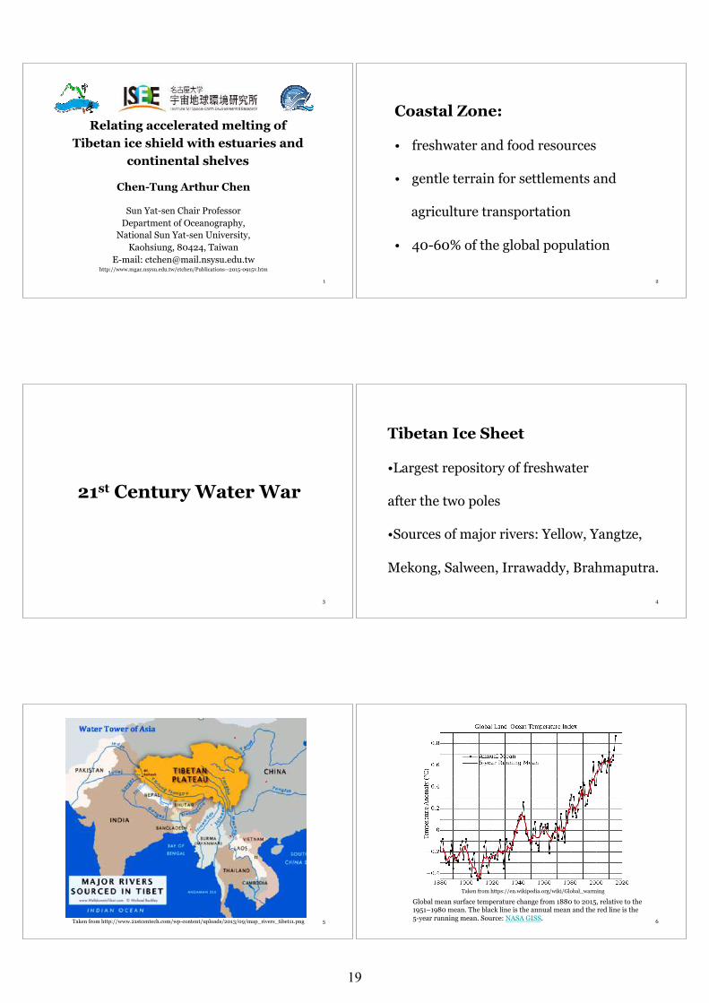
Coastal Zone:
• freshwater and food resources
• gentle terrain for settlements and
agriculture transportation
• 40-60% of the global population
3
21st Century Water War
4
Tibetan Ice Sheet
• Largest repository of freshwater
after the two poles
• Sources of major rivers: Yellow, Yangtze,
Mekong, Salween, Irrawaddy, Brahmaputra.
5 Taken from http://www.21stcentech.com/wp-content/uploads/2013/09/map_rivers_tibet11.png 6
Global mean surface temperature change from 1880 to 2015, relative to the 1951–1980 mean. The black line is the annual mean and the red line is the 5-year running mean. Source: NASA GISS.
Global mean surface temperature change from 1880 to 2015, relative to the 1951–1980 mean. The black line is the annual mean and the red line is the 5-year running mean. Source: NASA GISS.
Taken from https://en.wikipedia.org/wiki/Global_warming
19
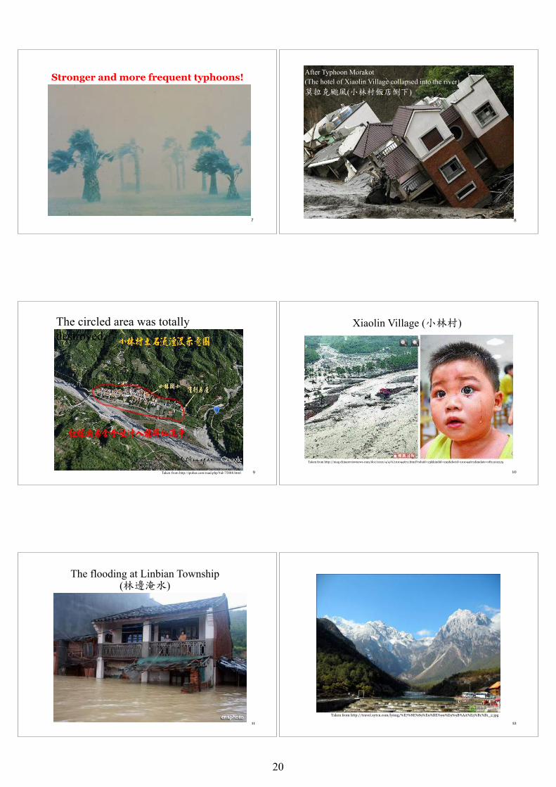
7
Stronger and more frequent typhoons!
8
After Typhoon Morakot (The hotel of Xiaolin Village collapsed into the river) ����(��� ��)
9 Taken from http://ipobar.com/read.php?tid-75888.html
The circled area was totally destroyed.
10
Xiaolin Village (���)
Taken from http://mag.chinareviewnews.com/doc/1010/4/4/6/101044672.html?coluid=23&kindid=292&docid=101044672&mdate=0811102225
11
The flooding at Linbian Township (����)
12
Taken from http://travel.xytcn.com/lyimg/%E7%8E%89%E9%BE%99%E9%9B%AA%E5%B1%B1_2.jpg
20
13
14
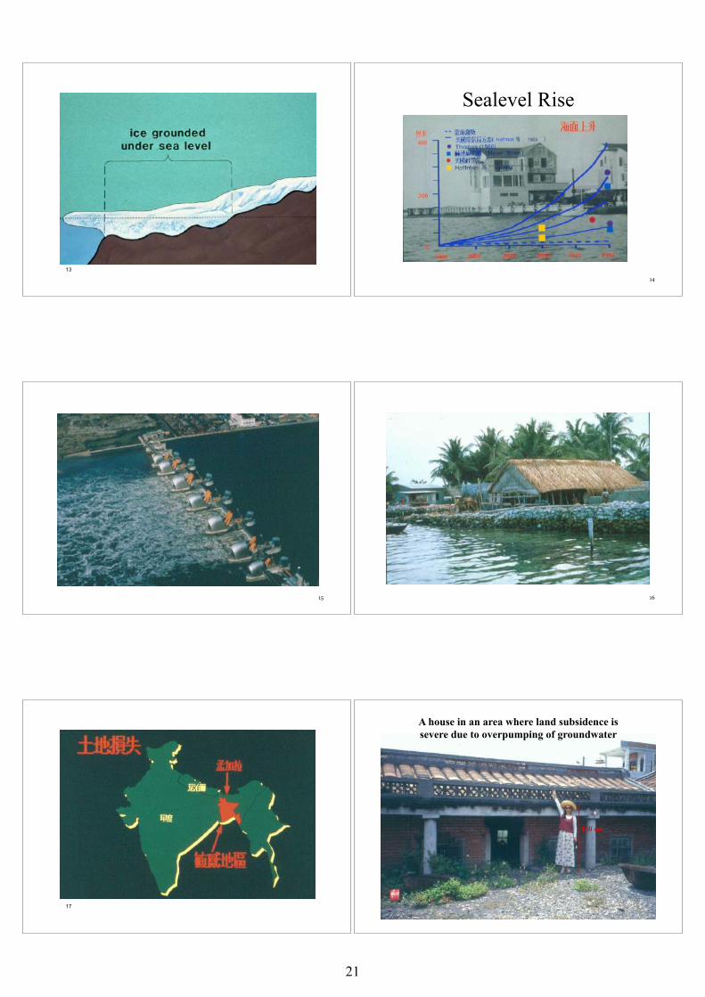
Sealevel Rise
15 16
17
18
A house in an area where land subsidence is severe due to overpumping of groundwater
160 cm
21
19
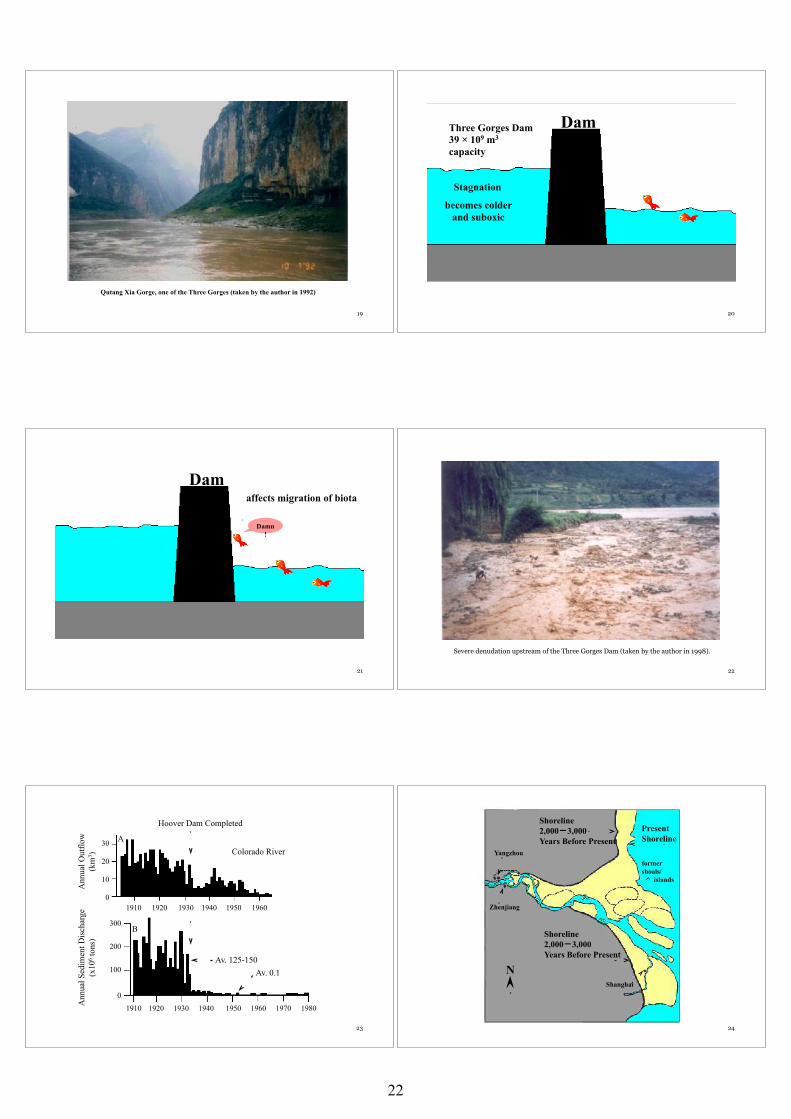
Qutang Xia Gorge, one of the Three Gorges (taken by the author in 1992)
20
becomes colder and suboxic
Dam
Stagnation
39 × 109 m3 capacity
Three Gorges Dam
21
affects migration of biota
Damn!
Dam
22
Severe denudation upstream of the Three Gorges Dam (taken by the author in 1998).
23
Hoover Dam Completed
Colorado River
Ann
ual S
edim
ent D
isch
arge
(x
106 t
ons)
A
B
Av. 125-150 Av. 0.1
Ann
ual O
utflo
w
(km
3 )
300
30
10
20
0
200
100
0
1910 1950 1960 1930 1940 1920
1910 1920 1930 1950 1940 1960 1970 1980
24
Shoreline 2,000-3,000 Years Before Present
Shoreline 2,000-3,000 Years Before Present
Yangzhou
Zhenjiang
Shanghai
former shoals/ islands
N
Present Shoreline
22
25
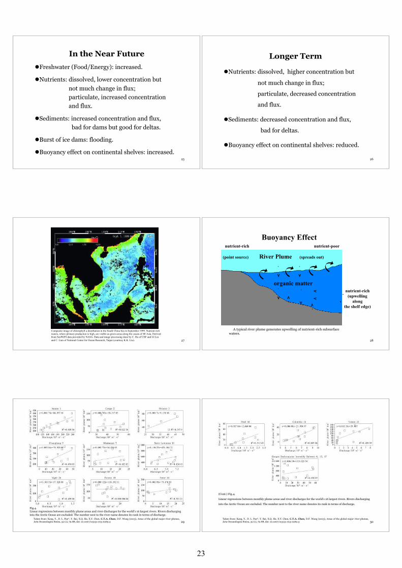
In the Near Future
! Freshwater (Food/Energy): increased.
! Nutrients: dissolved, lower concentration but not much change in flux; particulate, increased concentration and flux.
! Sediments: increased concentration and flux, bad for dams but good for deltas.
! Burst of ice dams: flooding.
! Buoyancy effect on continental shelves: increased. 26
Longer Term
! Nutrients: dissolved, higher concentration but
not much change in flux;
particulate, decreased concentration
and flux.
! Sediments: decreased concentration and flux,
bad for deltas.
! Buoyancy effect on continental shelves: reduced.
27
Composite image of chlorophyll a distribution in the South China Sea in September 1999. Nutrient rich waters, where primary production is high, are visible as green areas along the coasts of SE Asia. Derived from SeaWiFS data provided by NASA. Data and image processing done by C. Hu of USF and I-I Lin and C. Lian of National Center for Ocean Research, Taipei (courtesy K.K. Liu). 28
Buoyancy Effect
nutrient-rich nutrient-poor
organic matter
(point source) River Plume (spreads out)
nutrient-rich
(upwelling along
the shelf edge)
A typical river plume generates upwelling of nutrient-rich subsurface waters.
Taken from: Kang, Y., D. L. Pan*, Y. Bai, X.Q. He, X.Y. Chen, C.T.A. Chen, D.F. Wang (2013), Areas of the global major river plumes, Acta Oceanologica Sinica, 32 (1), 79-88, doi: 10.1007/s13131-013-0269-5
Fig.4. Linear regressions between monthly plume areas and river discharges for the world’s 16 largest rivers. Rivers discharging into the Arctic Ocean are excluded. The number next to the river name denotes its rank in terms of discharge.
29
(Cont.) Fig.4.
Linear regressions between monthly plume areas and river discharges for the world’s 16 largest rivers. Rivers discharging
into the Arctic Ocean are excluded. The number next to the river name denotes its rank in terms of discharge.
Taken from: Kang, Y., D. L. Pan*, Y. Bai, X.Q. He, X.Y. Chen, C.T.A. Chen, D.F. Wang (2013), Areas of the global major river plumes, Acta Oceanologica Sinica, 32 (1), 79-88, doi: 10.1007/s13131-013-0269-5 30
23
31
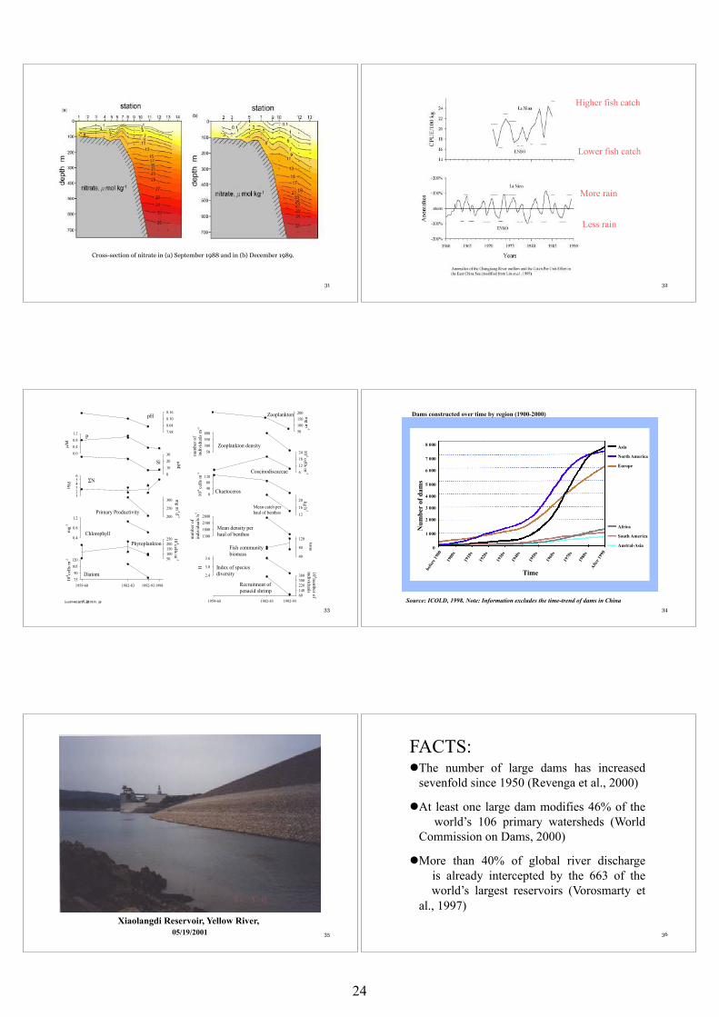
Cross-section of nitrate in (a) September 1988 and in (b) December 1989.
32
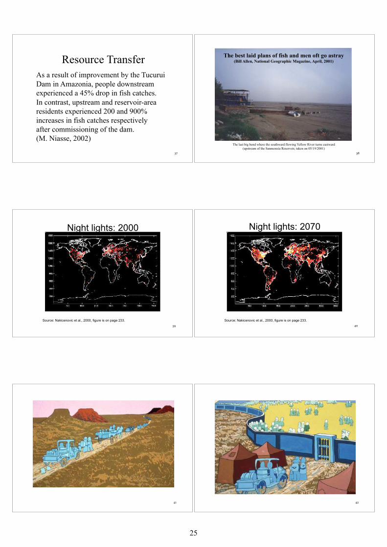
Higher fish catch
Lower fish catch
More rain
Less rain
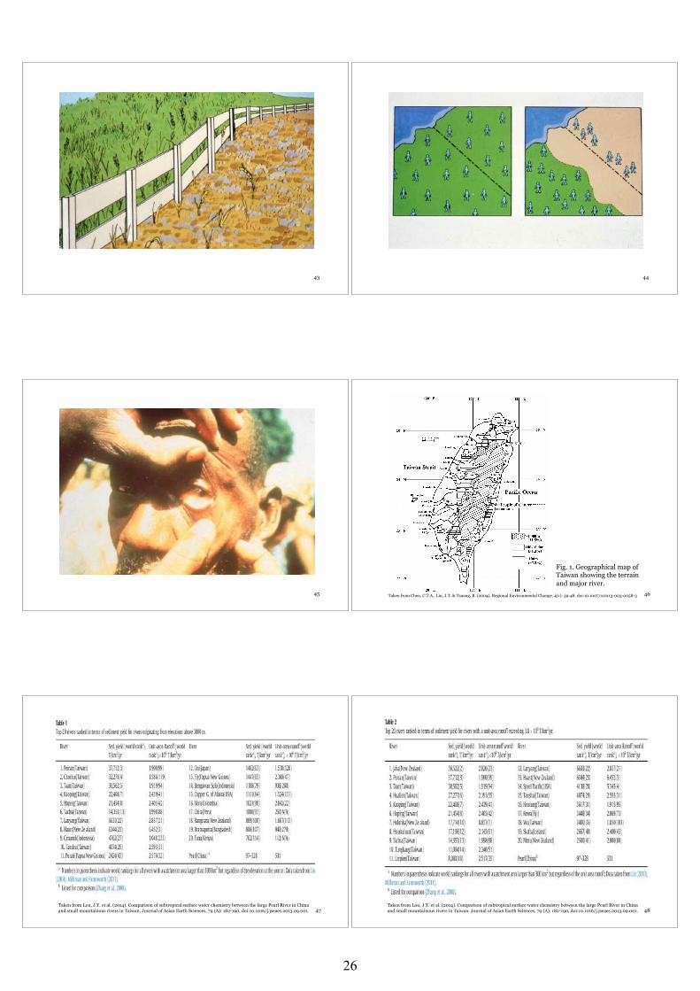
33
mg m
-3
50100150200
num
ber o
f in
divi
dual
s m
-3
50300550800
104 cells m
-36121824
104 c
ells
m-3
04080
120
12
16
20 kg h-1
num
ber o
f in
divi
dual
s h-1
1300180023002800
tons
40
80
120
H
2.4
3.0
3.6
1959-60 1982-83 1992-93
106num
ber of individuals
60140220300380
7.988.048.108.16
01020300.0
0.40.81.2
123456
200
250
300
mg-3
0.4
0.8
1.2
104cells m
-350100150200250
1959-60 1982-83 1992-93 1998 1
04 cells
m-3
7590
105120
pH
µΜ
µM m
g m-2d
-1
µΜ
lion804¥d:¥al¥����910830. jnb
P
Si
ΣN
Primary Productivity
Chlorophyll
Phytoplankton
Diatom
Zooplankton
Zooplankton density
Coscinodiscaceae
Chaetoceros
Mean catch per haul of benthos
Mean density per haul of benthos
Fish community biomass
Index of species diversity
Recruitment of penaeid shrimp
34
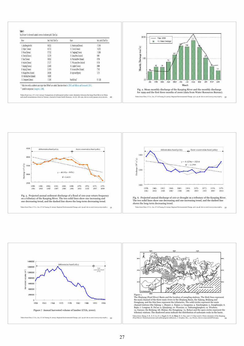
Dams constructed over time by region (1900-2000)
Source: ICOLD, 1998. Note: Information excludes the time-trend of dams in China
Time
Num
ber
of d
ams
Asia
North America
Europe
Africa
South America
Austral-Asia
8 000
7 000
6 000
5 000
4 000
3 000
2 000
1 000
0
35
Xiaolangdi Reservoir, Yellow River, 05/19/2001 36
FACTS: ! The number of large dams has increased sevenfold since 1950 (Revenga et al., 2000)
! At least one large dam modifies 46% of the world’s 106 primary watersheds (World Commission on Dams, 2000)
! More than 40% of global river discharge is already intercepted by the 663 of the world’s largest reservoirs (Vorosmarty et al., 1997)
24
37
Resource Transfer As a result of improvement by the Tucurui Dam in Amazonia, people downstream experienced a 45% drop in fish catches. In contrast, upstream and reservoir-area residents experienced 200 and 900% increases in fish catches respectively after commissioning of the dam. (M. Niasse, 2002)
38
The last big bend where the southward flowing Yellow River turns eastward (upstream of the Sanmenxia Reservoir, taken on 05/19/2001)
The best laid plans of fish and men oft go astray (Bill Allen, National Geographic Magazine, April, 2001)
39
Source: Nakicenovic et al., 2000, figure is on page 233.
Night lights: 2000
40
Source: Nakicenovic et al., 2000, figure is on page 233.
Night lights: 2070
41 42
25
43 44
45 46
Fig. 1. Geographical map of Taiwan showing the terrain and major river.
Taken from Chen, C.T.A., Liu, J.T. & Tsuang, B. (2004). Regional Environmental Change, 4(1): 39-48. doi:10.1007/s10113-003-0058-3
47 Taken from Lou, J.Y. et al. (2014). Comparison of subtropical surface water chemistry between the large Pearl River in China and small mountainous rivers in Taiwan. Journal of Asian Earth Sciences, 79 (A): 182-190, doi:10.1016/j.jseaes.2013.09.001.! 48
Taken from Lou, J.Y. et al. (2014). Comparison of subtropical surface water chemistry between the large Pearl River in China and small mountainous rivers in Taiwan. Journal of Asian Earth Sciences, 79 (A): 182-190, doi:10.1016/j.jseaes.2013.09.001.!
26
49 Taken from Lou, J.Y. et al. (2014). Comparison of subtropical surface water chemistry between the large Pearl River in China and small mountainous rivers in Taiwan. Journal of Asian Earth Sciences, 79 (A): 182-190, doi:10.1016/j.jseaes.2013.09.001.! 50
Fig. 2. Mean monthly discharge of the Kaoping River and the monthly discharge for 1999 and the first three months of 2000 (data from Water Resources Bureau).
Taken from Chen, C.T.A., Liu, J.T. & Tsuang, B. (2004). Regional Environmental Change, 4(1): 39-48. doi:10.1007/s10113-003-0058-3
51
Fig. 5. Projected annual sediment discharge of a flood of 100-year return frequency on a tributary of the Kaoping River. The two solid lines show one increasing and one decreasing trend, and the dashed line shows the long-term decreasing trend.
Taken from Chen, C.T.A., Liu, J.T. & Tsuang, B. (2004). Regional Environmental Change, 4(1): 39-48. doi:10.1007/s10113-003-0058-3
52
Fig. 6. Projected annual discharge of 100-yr drought on a tributary of the Kaoping River. The two solid lines show one decreasing and one increasing trend, and the dashed line shows the long-term decreasing trend.
Taken from Chen, C.T.A., Liu, J.T. & Tsuang, B. (2004). Regional Environmental Change, 4(1): 39-48. doi:10.1007/s10113-003-0058-3
53
Figure 7 Annual harvested volume of lumber (COA, 2000).
Taken from Chen, C.T.A., Liu, J.T. & Tsuang, B. (2004). Regional Environmental Change, 4(1): 39-48. doi:10.1007/s10113-003-0058-3
Figure 1. The Zhujiang (Pearl River) Basin and the location of sampling stations. The thick lines represent the main channel of the three main rivers in the Zhujiang Basin, the Xijiang, Beijiang and Dongjiang, and the thin lines represent the tributaries. The solid circles represent the main channel stations (the Xijiang: 1. Zhanyi; 2. Xiqiao; 3. Gaoguma; 4. Xiaolongtan; 5. Jiangbianjie; 6. Bajie; 7. Longtan; 8. Du'an; 9. Qianjiang; 10. Wuxuan; 11. Dahuangjiangkou; 12. Wuzhou; 13. Gaoyao; the Beijiang: 68. Shijiao; the Dongjiang: 73. Boluo) and the open circles represent the tributary stations. The shadowed areas indicate the distribution of carbonate rocks in the basin.
Taken from: Zhang, S.-R., X. X. Lu, D. L. Higgitt, C.-T. A. Chen, H.-G. Sun, and J.-T. Han (2007), Water chemistry of the Zhujiang (Pearl River): Natural processes and anthropogenic influences, J. Geophys. Res., 112, F01011, doi:10.1029/2006JF000493. 54
27
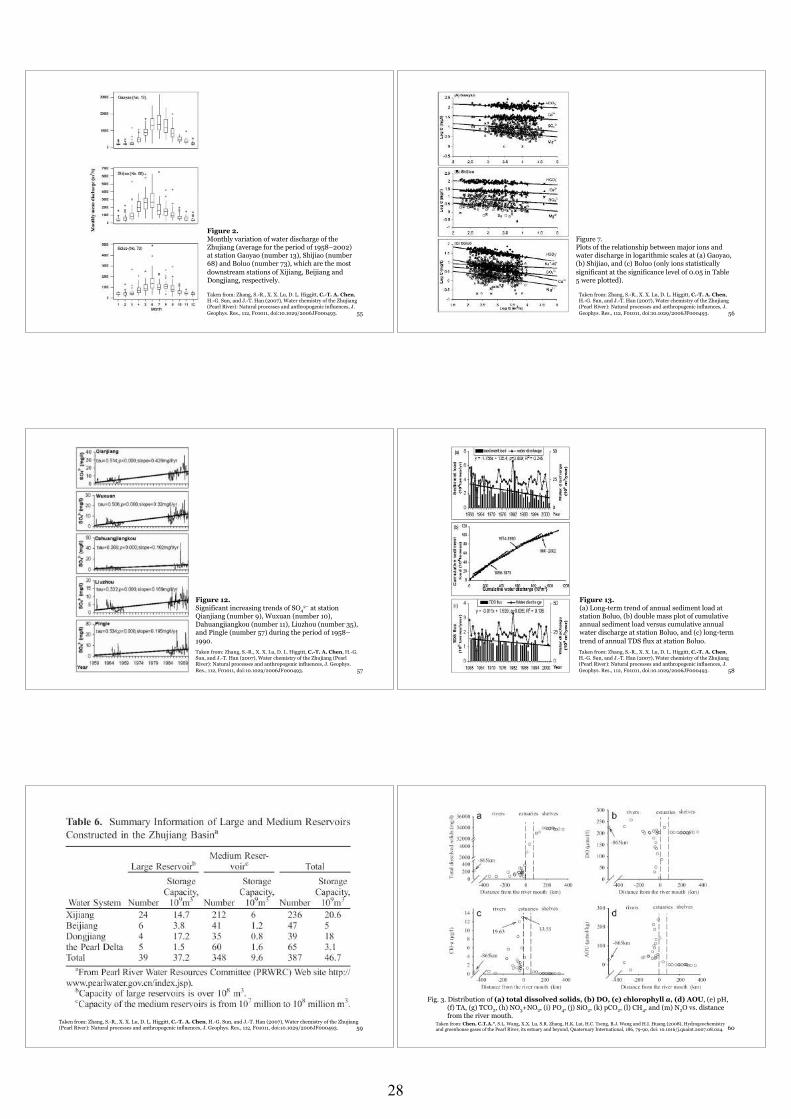
Figure 2. Monthly variation of water discharge of the Zhujiang (average for the period of 1958–2002) at station Gaoyao (number 13), Shijiao (number 68) and Boluo (number 73), which are the most downstream stations of Xijiang, Beijiang and Dongjiang, respectively.
Taken from: Zhang, S.-R., X. X. Lu, D. L. Higgitt, C.-T. A. Chen, H.-G. Sun, and J.-T. Han (2007), Water chemistry of the Zhujiang (Pearl River): Natural processes and anthropogenic influences, J. Geophys. Res., 112, F01011, doi:10.1029/2006JF000493. 55
Figure 7. Plots of the relationship between major ions and water discharge in logarithmic scales at (a) Gaoyao, (b) Shijiao, and (c) Boluo (only ions statistically significant at the significance level of 0.05 in Table 5 were plotted).
Taken from: Zhang, S.-R., X. X. Lu, D. L. Higgitt, C.-T. A. Chen, H.-G. Sun, and J.-T. Han (2007), Water chemistry of the Zhujiang (Pearl River): Natural processes and anthropogenic influences, J. Geophys. Res., 112, F01011, doi:10.1029/2006JF000493. 56
Figure 12. Significant increasing trends of SO4
2− at station Qianjiang (number 9), Wuxuan (number 10), Dahuangjiangkou (number 11), Liuzhou (number 35), and Pingle (number 57) during the period of 1958–1990. Taken from: Zhang, S.-R., X. X. Lu, D. L. Higgitt, C.-T. A. Chen, H.-G. Sun, and J.-T. Han (2007), Water chemistry of the Zhujiang (Pearl River): Natural processes and anthropogenic influences, J. Geophys. Res., 112, F01011, doi:10.1029/2006JF000493. 57
Figure 13. (a) Long-term trend of annual sediment load at station Boluo, (b) double mass plot of cumulative annual sediment load versus cumulative annual water discharge at station Boluo, and (c) long-term trend of annual TDS flux at station Boluo. Taken from: Zhang, S.-R., X. X. Lu, D. L. Higgitt, C.-T. A. Chen, H.-G. Sun, and J.-T. Han (2007), Water chemistry of the Zhujiang (Pearl River): Natural processes and anthropogenic influences, J. Geophys. Res., 112, F01011, doi:10.1029/2006JF000493. 58
Taken from: Zhang, S.-R., X. X. Lu, D. L. Higgitt, C.-T. A. Chen, H.-G. Sun, and J.-T. Han (2007), Water chemistry of the Zhujiang (Pearl River): Natural processes and anthropogenic influences, J. Geophys. Res., 112, F01011, doi:10.1029/2006JF000493. 59
Taken from: Chen, C.T.A.*, S.L. Wang, X.X. Lu, S.R. Zhang, H.K. Lui, H.C. Tseng, B.J. Wang and H.I. Huang (2008), Hydrogeochemistry and greenhouse gases of the Pearl River, its estuary and beyond, Quaternary International, 186, 79-90, doi: 10.1016/j.quaint.2007.08.024.
Fig. 3. Distribution of (a) total dissolved solids, (b) DO, (c) chlorophyll a, (d) AOU, (e) pH, (f) TA, (g) TCO2, (h) NO3+NO2, (i) PO4, (j) SiO2, (k) pCO2, (l) CH4, and (m) N2O vs. distance from the river mouth.
60
28
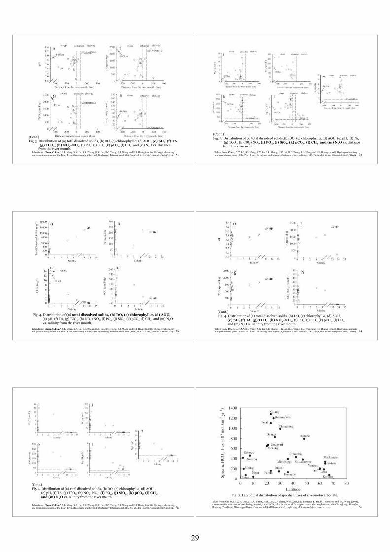
(Cont.) Fig. 3. Distribution of (a) total dissolved solids, (b) DO, (c) chlorophyll a, (d) AOU, (e) pH, (f) TA, (g) TCO2, (h) NO3+NO2, (i) PO4, (j) SiO2, (k) pCO2, (l) CH4, and (m) N2O vs. distance from the river mouth.
Taken from: Chen, C.T.A.*, S.L. Wang, X.X. Lu, S.R. Zhang, H.K. Lui, H.C. Tseng, B.J. Wang and H.I. Huang (2008), Hydrogeochemistry and greenhouse gases of the Pearl River, its estuary and beyond, Quaternary International, 186, 79-90, doi: 10.1016/j.quaint.2007.08.024. 61
(Cont.) Fig. 3. Distribution of (a) total dissolved solids, (b) DO, (c) chlorophyll a, (d) AOU, (e) pH, (f) TA, (g) TCO2, (h) NO3+NO2, (i) PO4, (j) SiO2, (k) pCO2, (l) CH4, and (m) N2O vs. distance from the river mouth.
Taken from: Chen, C.T.A.*, S.L. Wang, X.X. Lu, S.R. Zhang, H.K. Lui, H.C. Tseng, B.J. Wang and H.I. Huang (2008), Hydrogeochemistry and greenhouse gases of the Pearl River, its estuary and beyond, Quaternary International, 186, 79-90, doi: 10.1016/j.quaint.2007.08.024. 62
Taken from: Chen, C.T.A.*, S.L. Wang, X.X. Lu, S.R. Zhang, H.K. Lui, H.C. Tseng, B.J. Wang and H.I. Huang (2008), Hydrogeochemistry and greenhouse gases of the Pearl River, its estuary and beyond, Quaternary International, 186, 79-90, doi: 10.1016/j.quaint.2007.08.024.
Fig. 4. Distribution of (a) total dissolved solids, (b) DO, (c) chlorophyll a, (d) AOU, (e) pH, (f) TA, (g) TCO2, (h) NO3+NO2, (i) PO4, (j) SiO2, (k) pCO2, (l) CH4, and (m) N2O vs. salinity from the river mouth.
63 Taken from: Chen, C.T.A.*, S.L. Wang, X.X. Lu, S.R. Zhang, H.K. Lui, H.C. Tseng, B.J. Wang and H.I. Huang (2008), Hydrogeochemistry and greenhouse gases of the Pearl River, its estuary and beyond, Quaternary International, 186, 79-90, doi: 10.1016/j.quaint.2007.08.024.
(Cont.) Fig. 4. Distribution of (a) total dissolved solids, (b) DO, (c) chlorophyll a, (d) AOU, (e) pH, (f) TA, (g) TCO2, (h) NO3+NO2, (i) PO4, (j) SiO2, (k) pCO2, (l) CH4, and (m) N2O vs. salinity from the river mouth.
64
Taken from: Chen, C.T.A.*, S.L. Wang, X.X. Lu, S.R. Zhang, H.K. Lui, H.C. Tseng, B.J. Wang and H.I. Huang (2008), Hydrogeochemistry and greenhouse gases of the Pearl River, its estuary and beyond, Quaternary International, 186, 79-90, doi: 10.1016/j.quaint.2007.08.024.
(Cont.) Fig. 4. Distribution of (a) total dissolved solids, (b) DO, (c) chlorophyll a, (d) AOU, (e) pH, (f) TA, (g) TCO2, (h) NO3+NO2, (i) PO4, (j) SiO2, (k) pCO2, (l) CH4, and (m) N2O vs. salinity from the river mouth.
65
Fig. 2. Latitudinal distribution of specific fluxes of riverine bicarbonate.
Taken from: Cai, W.J.*, X.H. Guo, C.T.A. Chen, M.H. Dai, L.J. Zhang, W.D. Zhai, S.E. Lohrenz, K. Yin, P.J. Harrison and Y.C. Wang (2008), A comparative overview of weathering intensity and HCO3- flux in the world’s largest rivers with emphasis on the Changjiang, Huanghe, Zhujiang (Pearl) and Mississippi Rivers, Continental Shelf Research, 28, 1538-1549, doi: 10.1016/j.csr.2007.10.014. 66
29
Taken from: Chen, C.T.A.* (Arthur, C.C.T) (2008), Buoyancy leads to high productivity of the Changjiang Diluted Water: a note, Acta Oceanologica Sinica, 27 (6), 133-140.
Fig. 1. Annual fluxes of (a) water; (b) DIN; (c) NO3; (d) PO4 and (e) SiO2 of the Changjiang (Data taken from Shen, 2000a, b; Shen et al., 2001; Li et al., 2007). Since the DIN data are not continuous but those of NO3 are, the latter is also shown.
67
Taken from: Loh, P.S.*, C.T.A. Chen, J.Y. Lou, G.Z. Anshari, H.Y. Chen and J.T. Wang (2012), Comparing lignin-derived phenols, δ13C values, OC/N ratio and 14C age between sediments in the Kaoping (Taiwan) and the Kapuas (Kalimantan, Indonesia) Rivers, Aquatic Geochemistry, 18 (2), 141-158, doi: 10.1007/s10498-011-9153-0.
Fig. 3 δ13C values for the Kaoping and Kapuas Rivers. Open squares represent the Kapuas River during June–July 2007 sampling; open circles represent the Kapuas River during Dec 2007–Jan 2008 sampling; filled triangles (black) represent the tributaries draining into the Kaoping River; and shaded triangles (gray) represent the mainstream of the Kaoping River and three locations along its coastal zone.
68
Taken from: Loh, P.S.*, C.T.A. Chen, J.Y. Lou, G.Z. Anshari, H.Y. Chen and J.T. Wang (2012), Comparing lignin-derived phenols, δ13C values, OC/N ratio and 14C age between sediments in the Kaoping (Taiwan) and the Kapuas (Kalimantan, Indonesia) Rivers, Aquatic Geochemistry, 18 (2), 141-158, doi: 10.1007/s10498-011-9153-0.
Fig. 4 a molar OC/N ratios,b %OC and c %IC for the Kaoping and Kapuas Rivers. Open squares represent the Kapuas River during June–July 2007 sampling; open circles represent the Kapuas River during Dec 2007–Jan 2008 sampling; filled triangles (black) represent the tributaries draining into the Kaoping River; and shaded triangles (gray) represent the mainstream of the Kaoping River and three locations along its coastal zone
69 Taken from: Huang, T.H., Y.H. Fu, P.Y. Pan and C.T. A. Chen* (2012), Fluvial carbon fluxes in tropical rivers, Current Opinion in Environmental Sustainability, 4 (2), 162–169, doi: 10.1016/j.cosust.2012.02.004.
Figure 3. Latitudinal distribution of (a) DIC and carbonate outcrop areas (data from http://web.env.auckland.ac.nz/ our_research/karst/) and (b) DOC concentrations and soil organic carbon density.
70
71
Welcome to visit National Sun Yat-sen University
Taken from http://www.uu1.com/sight/cq1486.html
30
L1: River Discharge Kenji Tanaka (Disaster Prevention Research Institute, Kyoto University) Abstract
River discharge is an important source of freshwater supply to oceans. According to the global estimates, precipitation over oceans is approximately 391 thousand Gt per year, while river discharge is approximately 45.5 thousand Gt per year. Amount of river discharge changes greatly as consequences of climate, vegetation, soil type, drainage basin relief and the human activities, etc. As river discharge is not measured at all rivers, hydrological model is necessary to estimate the global freshwater supply from global land areas to oceans. There are various kinds of hydrological models to calculate river discharge. In some applications focusing on peak discharge analysis or flood forecasting, land surface processes can be neglected. As the time and spatial scale increases, land surface processes become more and more important, especially, in the area where evapotranspiration is a dominant component.
In this training course, in-land water cycle model which consists of land surface model, river routing model, irrigation model, reservoir operation model is introduced to show you how time and spatial distribution of river discharge is calculated. Current achievement, difficulties, new challenges in large scale model are introduced.
31

32
Lecture 1River Discharge
Kenji TanakaWater Resources Research Center
Disaster Prevention Research Institute, Kyoto University, Japan
26th IHP Training Course (2016/11/28)
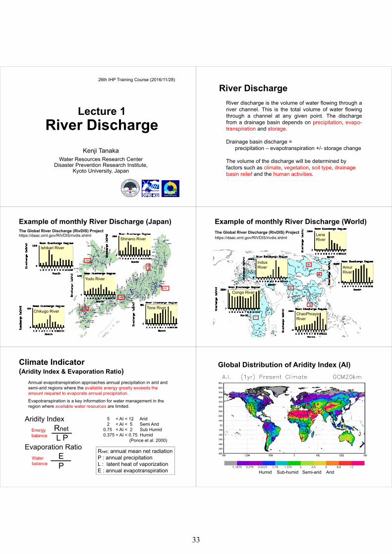
River DischargeRiver discharge is the volume of water flowing through ariver channel. This is the total volume of water flowingthrough a channel at any given point. The dischargefrom a drainage basin depends on precipitation, evapo-transpiration and storage.
Drainage basin discharge = precipitation – evapotranspiration +/- storage change
The volume of the discharge will be determined by factors such as climate, vegetation, soil type, drainage basin relief and the human activities.
Yodo River
Tone RiverChikugo River
Shinano River
Ishikari River
Example of monthly River Discharge (Japan)
https://daac.ornl.gov/RIVDIS/rivdis.shtmlThe Global River Discharge (RivDIS) Project
Example of monthly River Discharge (World)
IndusRiver
LenaRiver
AmurRiver
ChaoPhrayaRiver
Congo River
https://daac.ornl.gov/RIVDIS/rivdis.shtmlThe Global River Discharge (RivDIS) Project
Annual evapotranspiration approaches annual precipitation in arid and semi-arid regions where the available energy greatly exceeds the amount required to evaporate annual precipitation. Evapotranspiration is a key information for water management in the region where available water resources are limited.
Climate Indicator (Aridity Index & Evaporation Ratio)
Aridity IndexRnetL P
Evaporation RatioE P
Rnet: annual mean net radiationP : annual precipitationL : latent heat of vaporizationE : annual evapotranspiration
5 < AI < 12 Arid2 < AI < 5 Semi Arid
0.75 < AI < 2 Sub Humid0.375 < AI < 0.75 Humid
(Ponce et al. 2000)
Energybalance
Waterbalance
Humid Sub-humid Semi-arid Arid
Global Distribution of Aridity Index (AI)
33
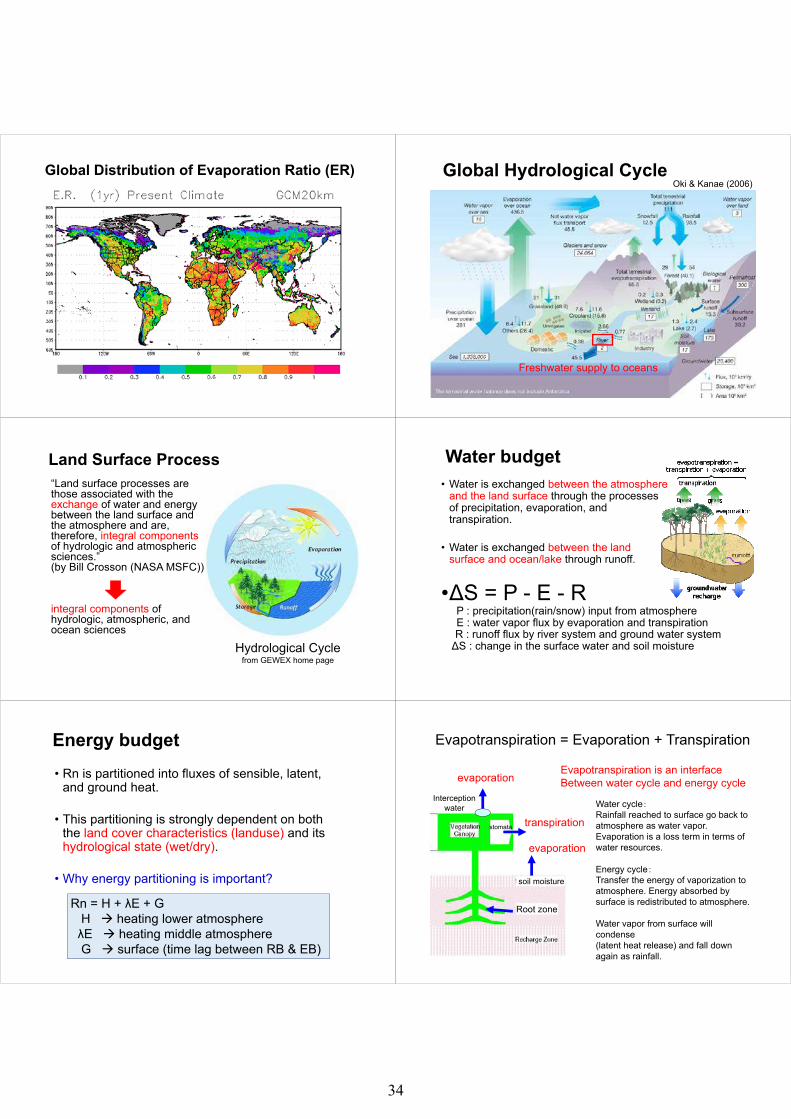
Global Distribution of Evaporation Ratio (ER) Global Hydrological Cycle Oki & Kanae (2006)
Freshwater supply to oceans
Land Surface Process“Land surface processes are those associated with the exchange of water and energy between the land surface and the atmosphere and are, therefore, integral components of hydrologic and atmospheric sciences.”(by Bill Crosson (NASA MSFC))
integral components of hydrologic, atmospheric, and ocean sciences
Hydrological Cyclefrom GEWEX home page
Water budget• Water is exchanged between the atmosphere
and the land surface through the processes of precipitation, evaporation, and transpiration.
• Water is exchanged between the land surface and ocean/lake through runoff.
•ΔS = P - E - R P : precipitation(rain/snow) input from atmosphereE : water vapor flux by evaporation and transpirationR : runoff flux by river system and ground water system
ΔS : change in the surface water and soil moisture
Energy budget• Rn is partitioned into fluxes of sensible, latent,
and ground heat.
• This partitioning is strongly dependent on both the land cover characteristics (landuse) and its hydrological state (wet/dry).
• Why energy partitioning is important?
Rn = H + λE + G H heating lower atmosphereλE heating middle atmosphereG surface (time lag between RB & EB)
Evapotranspiration = Evaporation + Transpiration
Root zone
stomata transpiration
evaporation
evaporation
Interceptionwater
soil moisture
Evapotranspiration is an interface Between water cycle and energy cycle
Water cycle:Rainfall reached to surface go back to atmosphere as water vapor. Evaporation is a loss term in terms of water resources.
Energy cycle:Transfer the energy of vaporization to atmosphere. Energy absorbed by surface is redistributed to atmosphere.
Water vapor from surface will condense (latent heat release) and fall down again as rainfall.
34
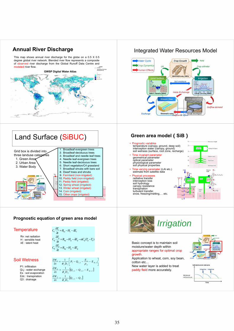
Annual River DischargeThis map shows annual river discharge for the globe on a 0.5 X 0.5degree global river network. Blended river flow represents a compositeof observed river discharge from the Global Runoff Data Centre andmodeled river flow.
GWSP Digital Water Atlas
Crop Dynamics
Human Effects
Water Cycle
Integrated Water Resources Model
Grid box is divided intothree landuse categories1. Green Area2. Urban Area3. Water Body
Simple Biosphere including UrbanCanopy
Land Surface (SiBUC)1.Broadleaf-evergreen trees2.Broadleaf-deciduous trees3.Broadleaf and needle leaf trees4.Needle leaf-evergreen trees5.Needle leaf-deciduous trees6.Short vegetation/C4 grassland7.Broadleaf shrubs with bare soil8.Dwarf trees and shrubs9.Farmland (non-irrigated)10. Paddy field (non-irrigated)11. Paddy field (irrigated)12. Spring wheat (irrigated)13. Winter wheat (irrigated)14. Corn (irrigated)15. Other crops (irrigated)
Green area model(SiB)• Prognostic variables
temperature (canopy, ground, deep soil)interception water (canopy, ground)soil wetness (surface, root zone, recharge)
• Time invariant parametergeometrical parameteroptical parameterphysiological parametersoil physical properties
• Time varying parameter (LAI etc.)estimate from satellite data
• Physical processesradiative transferinterception losssoil hydrologycanopy resistancetranspirationturbulent transfer,snow, freezing/melting,… etc.
Prognostic equation of green area model
ggngd
d
dggggngg
g
ccncc
c
EHRtTC
TTCEHRtT
C
EHRtTC
λ
ωλ
λ
−−=∂
∂
−−−−=∂
∂
−−=∂∂
)(
[ ]
[ ]33,23
3
2,3,22,12
2
1,2,111
1
1
1
1
QQDt
W
EQQDt
W
EEQPDt
W
s
dcs
dcw
s
s
−=∂
∂
−−=∂
∂
⎥⎦
⎤⎢⎣
⎡−−−=
∂∂
θ
θ
ρθ
Temperature
Soil Wetness
Rn: net radiationH : sensible heatλE : latent heat
P1: infiltrationQi,j : water exchangeEs : soil evaporationEdc : transpirationQ3 : drainage
Irrigation
Basic concept is to maintain soil moisture/water depth within appropriate ranges for optimal crop growth.Application to wheat, corn, soy bean, cotton etc…New water layer is added to treatpaddy field more accurately.
35
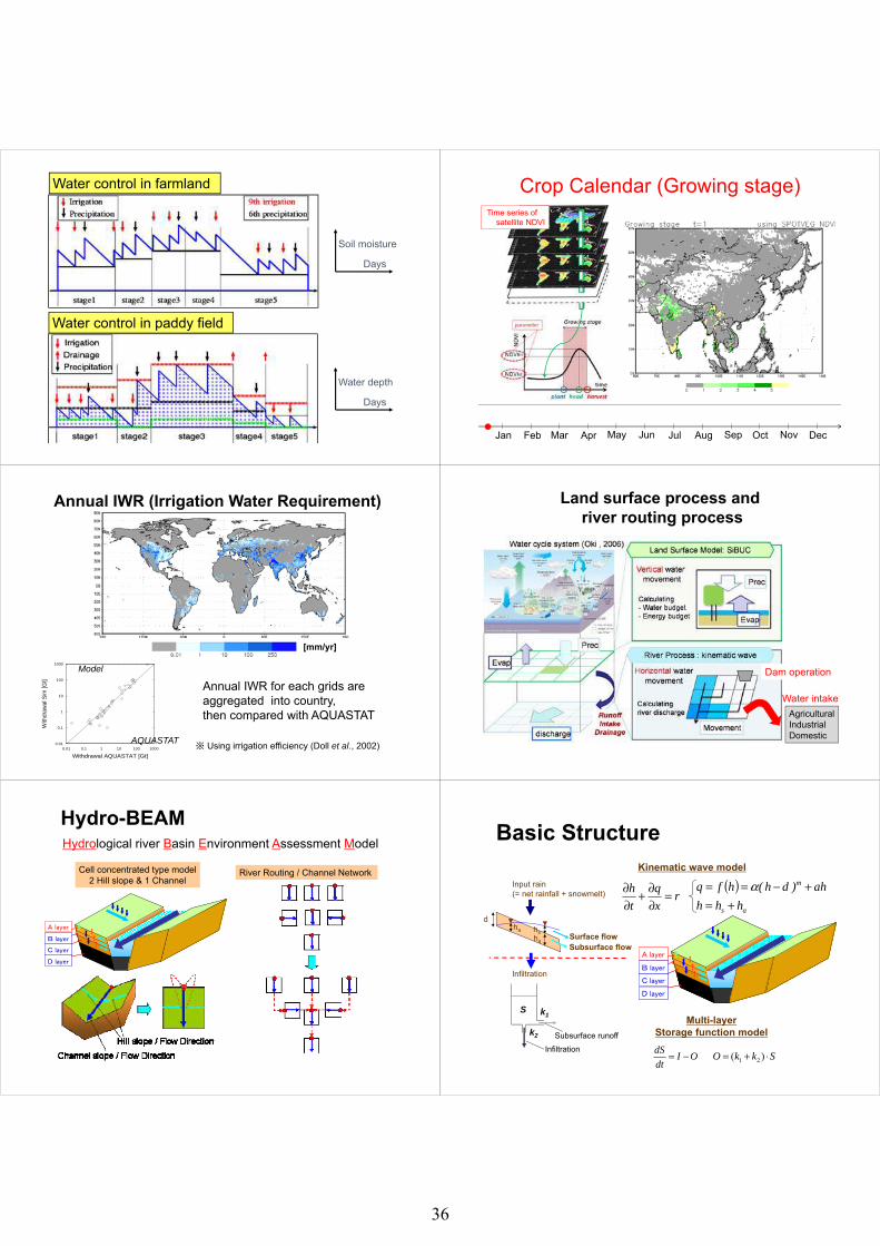
Water control in paddy field
Water depth
Days
Soil moisture
Days
Water control in farmland Crop Calendar (Growing stage)
Jan Feb Mar Apr May Jun Jul Aug Sep Oct Nov Dec
Time series of satellite NDVI
Annual IWR (Irrigation Water Requirement)
Annual IWR for each grids are aggregated into country, then compared with AQUASTAT
1000
100
10
1
0.1
0.0110001001010.10.01
With
draw
al S
im [G
t]
Withdrawal AQUASTAT [Gt]
Model
AQUASTAT※ Using irrigation efficiency (Doll et al., 2002)
[mm/yr]
Land surface process andriver routing process
AgriculturalIndustrialDomestic
Water intake
Dam operation
A layer
D layer
C layer
B layer
A layer
D layer
C layer
B layer
A layer
D layer
C layer
B layer
A layer
D layer
C layer
B layer
Cell concentrated type model2 Hill slope & 1 Channel
River Routing / Channel Network
Hydrological river Basin Environment Assessment Model
Hydro-BEAM Basic Structure
A layer
D layer
C layer
B layer
A layer
D layer
C layer
B layer
A layer
D layer
C layer
B layer
A layer
D layer
C layer
B layer
d
Input rain (= net rainfall + snowmelt)
Surface flowSubsurface flow
Kinematic wave model
Multi-layerStorage function model
rxq
th =
∂∂+
∂∂ ( )
as
m
hhhah)dh(hfq
+=+−== α
hsha
ha
Infiltration
OIdtdS −= SkkO ⋅+= )( 21
S k1
k2
InfiltrationSubsurface runoff
36
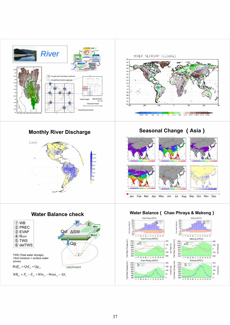
River
Monthly River Discharge Seasonal Change (Asia)
Jan Feb Mar Apr May Jun Jul Aug Sep Oct Nov Dec
① WB② PREC③ EVAP④ ROFF
⑤ TWS⑥ delTWS
Water Balance check
, , , , ,i t i t i t i t i t iWB P E Win Wout S= − + − − Δ
catchment
P E
ΔSW
i
Qsf
Qg
win
wout
, , ,i t i t i tRoff Qsf Qg= +
TWS (Total water storage)=Soil moisture + surface water (snow)
Water Balance( Chao Phraya & Mekong)
37
0
2000
4000
6000
8000
10000
12000
14000
DNOSAJJMAMFJ
RIV=BLUE NILE STA=ROSEIRES DAM
obsnodamdamin
0
1000
2000
3000
4000
5000
6000
DNOSAJJMAMFJ
RIV=SANAGA STA=EDEA
obsnodamdamin
0
500
1000
1500
2000
2500
DNOSAJJMAMFJ
RIV=CHAO PHRAYA STA=NAKHON SAWAN
obsnodamdamin
0
5000
10000
15000
20000
25000
30000
35000
40000
DNOSAJJMAMFJ
RIV=MEKONG STA=PHNOM PENH (CHRO
obsnodamdamin
0
5000
10000
15000
20000
25000
30000
35000
40000
45000
DNOSAJJMAMFJ
RIV=GANGES STA=FARAKKA
obsnodamdamin
0
2000
4000
6000
8000
10000
12000
14000
16000
DNOSAJJMAMFJ
RIV=ANGARA STA=BOGUCHANY
obsnodamdamin
0
500
1000
1500
2000
2500
3000
DNOSAJJMAMFJ
RIV=TIGRIS STA=BAGHDAD
obsnodamdamin
0
1000
2000
3000
4000
5000
6000
7000
8000
9000
DNOSAJJMAMFJ
RIV=CHURCHILL RIVER STA=BELOW FIDLER LA
obsnodamdamin
AS C
0
1000
2000
3000
4000
5000
6000
DNOSAJJMAMFJ
RIV=WINNIPEG RIVER STA=SLAVE FALLS
obsnodamdamin
0
1000
2000
3000
4000
5000
6000
7000
8000
DNOSAJJMAMFJ
RIV=SAO FRANCISCO STA=JUAZEIRO
obsnodamdamin
60000 80000
100000 120000 140000 160000 180000 200000 220000 240000 260000
DNOSAJJMAMFJ
RIV=AMAZONAS STA=OBIDOS
obsnodamdamin
1000
2000
3000
4000
5000
6000
7000
8000
9000
DNOSAJJMAMFJ
RIV=RIO JURUA STA=GAVIAO
obsnodamdamin
× Obs. Sim (dam) Sim (nodam)
-1
-0.5
0
0.5
1
1.5
2
0 0.2 0.4 0.6 0.8 1
BIAS
Evap/Prec
Dry region
Wet region
Overestimate in dry region
Dry index
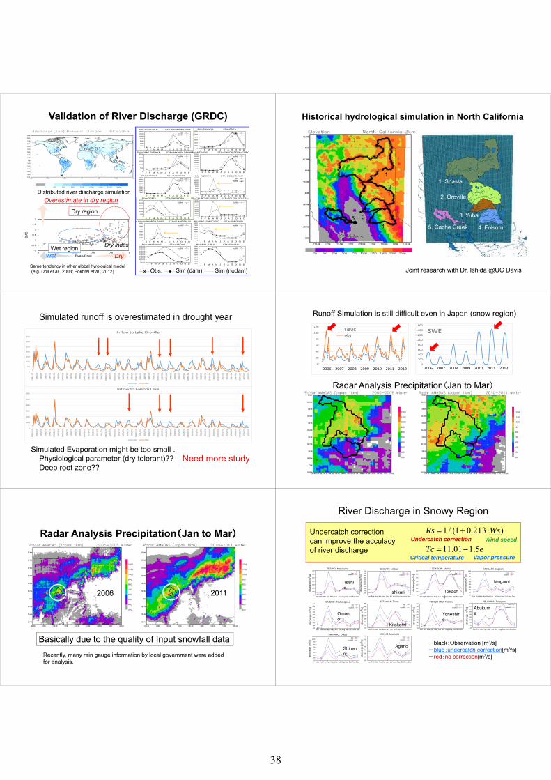
Distributed river discharge simulation
Same tendency in other global hyrological model(e.g. Doll et al., 2003; Pokhrel et al., 2012)
Validation of River Discharge (GRDC)
DryWet
1
43
2
5
1. Shasta
4. Folsom
2. Oroville
3. Yuba
5. Cache Creek
Historical hydrological simulation in North California
Joint research with Dr, Ishida @UC Davis
0
100
200
300
400
500
600
1994
/11/1
1995
/4/1
1995
/9/1
1996
/2/1
1996
/7/1
1996
/12/1
1997
/5/1
1997
/10/1
1998
/3/1
1998
/8/1
1999
/1/1
1999
/6/1
1999
/11/1
2000
/4/1
2000
/9/1
2001
/2/1
2001
/7/1
2001
/12/1
2002
/5/1
2002
/10/1
2003
/3/1
2003
/8/1
2004
/1/1
2004
/6/1
2004
/11/1
2005
/4/1
2005
/9/1
2006
/2/1
2006
/7/1
2006
/12/1
2007
/5/1
2007
/10/1
2008
/3/1
2008
/8/1
2009
/1/1
2009
/6/1
2009
/11/1
2010
/4/1
2010
/9/1
2011
/2/1
2011
/7/1
2011
/12/1
2012
/5/1
2012
/10/1
2013
/3/1
2013
/8/1
2014
/1/1
2014
/6/1
2014
/11/1
2015
/4/1
2015
/9/1
Inflow to Folsom Lake
Sim Obs
0
50
100
150
200
250
300
350
1994
/11/1
1995
/4/1
1995
/9/1
1996
/2/1
1996
/7/1
1996
/12/1
1997
/5/1
1997
/10/1
1998
/3/1
1998
/8/1
1999
/1/1
1999
/6/1
1999
/11/1
2000
/4/1
2000
/9/1
2001
/2/1
2001
/7/1
2001
/12/1
2002
/5/1
2002
/10/1
2003
/3/1
2003
/8/1
2004
/1/1
2004
/6/1
2004
/11/1
2005
/4/1
2005
/9/1
2006
/2/1
2006
/7/1
2006
/12/1
2007
/5/1
2007
/10/1
2008
/3/1
2008
/8/1
2009
/1/1
2009
/6/1
2009
/11/1
2010
/4/1
2010
/9/1
2011
/2/1
2011
/7/1
2011
/12/1
2012
/5/1
2012
/10/1
2013
/3/1
2013
/8/1
2014
/1/1
2014
/6/1
2014
/11/1
2015
/4/1
2015
/9/1
Inflow to Lake Oroville
Sim Obs
Simulated runoff is overestimated in drought year
Simulated Evaporation might be too small .Physiological parameter (dry tolerant)??Deep root zone??
Need more study
0
20
40
60
80
100
120SiBUCobs
2006 2007 2008 2009 2010 2011 20120
200
400
600
800
1000
1200
1400
1600
SWE
2006 2007 2008 2009 2010 2011 2012
Runoff Simulation is still difficult even in Japan (snow region)
Radar Analysis Precipitation(Jan to Mar)
Radar Analysis Precipitation(Jan to Mar)
20112006
Basically due to the quality of Input snowfall dataRecently, many rain gauge information by local government were added for analysis.
50
100
150
200
250
300
350
400
450
500
DecNovOctSepAugJulJunMayAprMarFebJan
disc
harg
e [m
3 /s]
YONESHIRO: Futatsuiobsrow
modified
50
100
150
200
250
300
350
400
DecNovOctSepAugJulJunMayAprMarFebJan
disc
harg
e [m
3 /s]
TOKACHI: Moiwaobsrow
modified
0
100
200
300
400
500
600
700
DecNovOctSepAugJulJunMayAprMarFebJan
disc
harg
e [m
3 /s]
TESHIO: Maruyamaobsrow
modified
200
300
400
500
600
700
800
900
1000
1100
DecNovOctSepAugJulJunMayAprMarFebJan
disc
harg
e [m
3 /s]
SHINANO: Odiyaobsrow
modified
100
150
200
250
300
350
400
450
500
550
DecNovOctSepAugJulJunMayAprMarFebJan
disc
harg
e [m
3 /s]
OMONO: Tsubakigawaobsrow
modified
100
200
300
400
500
600
700
800
900
1000
DecNovOctSepAugJulJunMayAprMarFebJan
disc
harg
e [m
3 /s]
MOGAMI: Sagoshiobsrow
modified
150
200
250
300
350
400
450
500
550
DecNovOctSepAugJulJunMayAprMarFebJan
disc
harg
e [m
3 /s]
KITAKAMI: Tomeobsrow
modified
0
100
200
300
400
500
600
700
800
900
1000
1100
DecNovOctSepAugJulJunMayAprMarFebJan
disc
harg
e [m
3 /s]
ISHIKARI: Ishikariobsrow
modified
100
200
300
400
500
600
700
800
DecNovOctSepAugJulJunMayAprMarFebJan
disc
harg
e [m
3 /s]
AGANO: Maoroshiobsrow
modified
40
60
80
100
120
140
160
180
200
220
DecNovOctSepAugJulJunMayAprMarFebJan
disc
harg
e [m
3 /s]
ABUKUMA: Tateyamaobsrow
modified
River Discharge in Snowy Region
-black:Observation [m3/s]-blue:undercatch correction[m3/s]-red:no correction[m3/s]
Undercatch correctioncan improve the acculacyof river discharge
1 / (1 0.213 )Rs Ws= + ⋅Undercatch correction Wind speed
Teshio
Agano
Ishikari
Omono
Mogami
Tokachi
AbukumaYoneshir
oKitakami
Shinano
11.01 1.5Tc e= −Vapor pressureCritical temperature
38
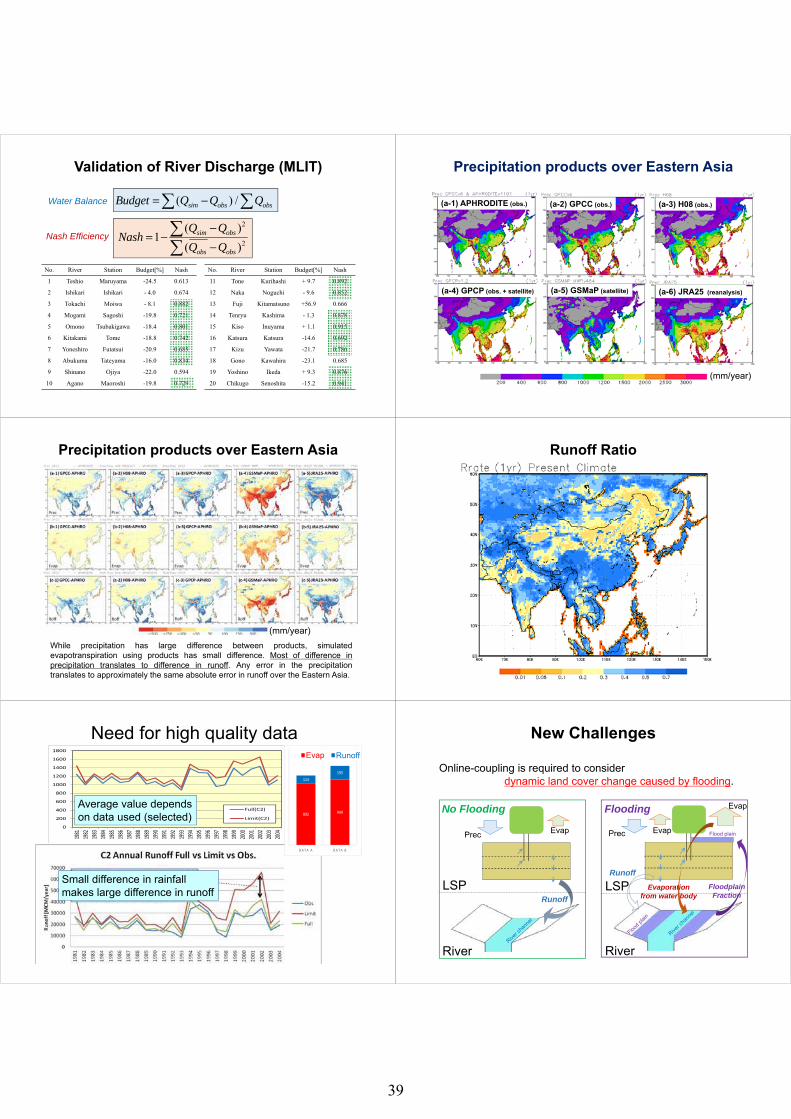
Validation of River Discharge (MLIT)
No. River Station Budget[%] Nash No. River Station Budget[%] Nash
1 Teshio Maruyama -24.5 0.613 11 Tone Kurihashi + 9.7 0.892
2 Ishikari Ishikari - 4.0 0.674 12 Naka Noguchi - 9.6 0.852
3 Tokachi Moiwa - 8.1 0.882 13 Fuji Kitamatsuno +56.9 0.666
4 Mogami Sagoshi -19.8 0.721 14 Tenryu Kashima - 1.3 0.878
5 Omono Tsubakigawa -18.4 0.801 15 Kiso Inuyama + 1.1 0.915
6 Kitakami Tome -18.8 0.742 16 Katsura Katsura -14.6 0.692
7 Yoneshiro Futatsui -20.9 0.685 17 Kizu Yawata -21.7 0.786
8 Abukuma Tateyama -16.0 0.834 18 Gono Kawahira -23.1 0.685
9 Shinano Ojiya -22.0 0.594 19 Yoshino Ikeda + 9.3 0.876
10 Agano Maoroshi -19.8 0.729 20 Chikugo Senoshita -15.2 0.941
( ) /sim obs obsBudget Q Q Q= −∑ ∑
Nash Efficiency
Water Balance
2
2
( )1
( )sim obs
obs obs
Q QNash
Q Q−
= −−
∑∑
Precipitation products over Eastern Asia
(a-1) APHRODITE (obs.) (a-2) GPCC (obs.) (a-3) H08 (obs.)
(a-4) GPCP (obs. + satellite) (a-5) GSMaP (satellite) (a-6) JRA25 (reanalysis)
(mm/year)
Precipitation products over Eastern Asia
While precipitation has large difference between products, simulatedevapotranspiration using products has small difference. Most of difference inprecipitation translates to difference in runoff. Any error in the precipitationtranslates to approximately the same absolute error in runoff over the Eastern Asia.
(mm/year)
Runoff Ratio
0
200
400
600
800
1000
1200
1400
1600
1800
1981
1982
1983
1984
1985
1986
1987
1988
1989
1990
1991
1992
1993
1994
1995
1996
1997
1998
1999
2000
2001
2002
2003
2004
Full(C2)
Limit(C2)
Need for high quality data
Average value depends on data used (selected)
Small difference in rainfall makes large difference in runoff
892 949
113195
D A T A A D A T A B
系列1 系列2Evap Runoff
New Challenges
Evap
No Flooding Flooding
Runoff
Flood plain
RunoffFloodplain Fraction
Evap
Evap
Evaporation from water body
Online-coupling is required to consider dynamic land cover change caused by flooding.
Prec Prec
LSP
River
LSP
River
39
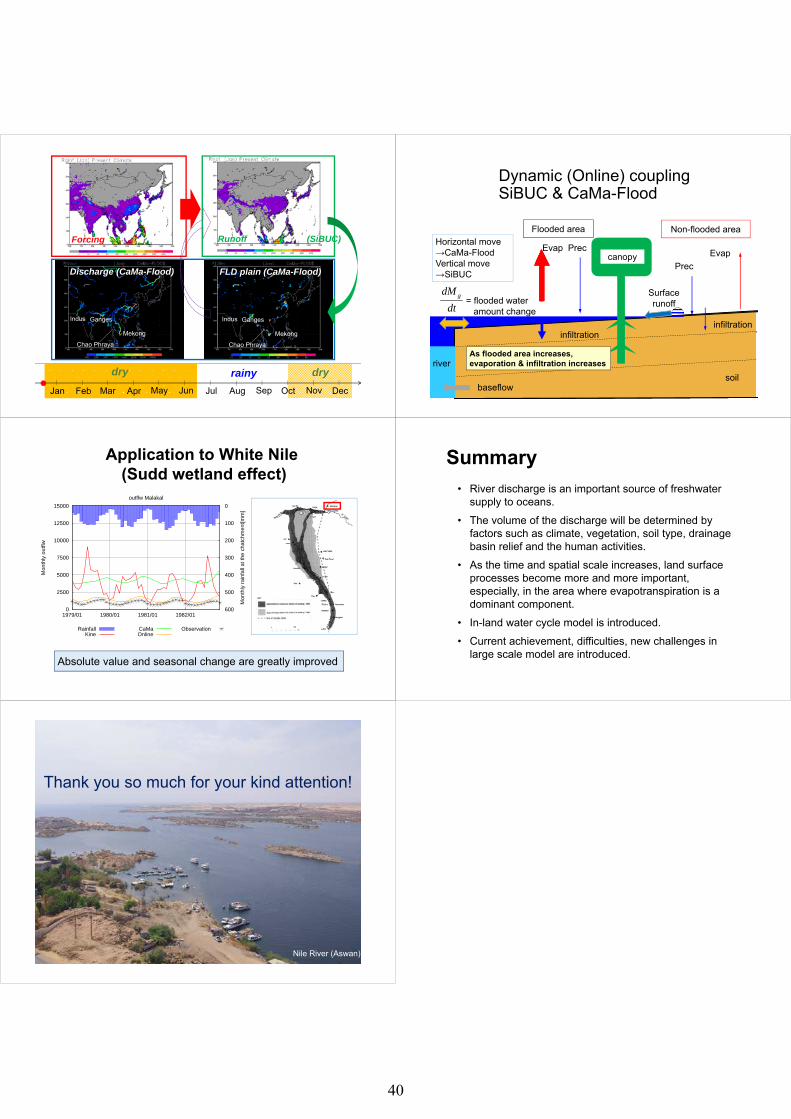
Jan Feb Mar Apr May Jun Jul Aug Sep Oct Nov Dec
dry dryrainy
Forcing Runoff (SiBUC)
Discharge (CaMa-Flood) FLD plain (CaMa-Flood)
Ganges
Mekong
Indus
Chao Phraya
Ganges
Mekong
Indus
Chao Phraya
Dynamic (Online) coupling SiBUC & CaMa-Flood
Flooded area
soilbaseflow
canopy
river
Non-flooded area
PrecEvapEvap Prec
infiltrationinfiltration
Surface runoff
gdMdt
= flooded water amount change
Horizontal move→CaMa-FloodVertical move →SiBUC
As flooded area increases, evaporation & infiltration increases
0
2500
5000
7500
10000
12500
15000
1979/01 1980/01 1981/01 1982/01
0
100
200
300
400
500
600
Mon
thly
out
flw
Mon
thly
rai
nfal
l at t
he c
hatc
hmen
t[mm
]
outflw Malakal
RainfallKine
CaMaOnline
Observation
Application to White Nile(Sudd wetland effect)
Absolute value and seasonal change are greatly improved
Summary• River discharge is an important source of freshwater
supply to oceans.• The volume of the discharge will be determined by
factors such as climate, vegetation, soil type, drainage basin relief and the human activities.
• As the time and spatial scale increases, land surface processes become more and more important, especially, in the area where evapotranspiration is a dominant component.
• In-land water cycle model is introduced.• Current achievement, difficulties, new challenges in
large scale model are introduced.
Thank you so much for your kind attention!
Nile River (Aswan)
40
L2: Submarine groundwater discharge from land to the ocean
Makoto Taniguchi (Research Institute for Humanity and Nature, Kyoto, Japan)
Submarine groundwater discharge (SGD) is a hidden pathway of water and dissolved
material from land to the ocean. Interdisciplinary research by hydrologists and
oceanographers during the last decay revealed less terrestrial SGD but huge material
flux by total SGD including re-circulated SGD. Spatial and temporal variations in
SGD were evaluated in site by direct measurements including seepage meters, 222Rn,
resistivity and others, as well as numerical simulations. Global estimates of SGD and
evaluations of impact of SGD on coastal ecosystem and fisheries are next future
research areas which are related to SGD.
41

42
1
Interactions Between Groundwater and Seawater in Permeable Sediments
Makoto TaniguchiResearch Institute for Humanity and Nature (RIHN)
Submarine Groundwater Discharge- Another pathway of water and dissolved materials
from land to the ocean -
Freshwater →(Hydrologists)
← Seawater(Oceanographers)
Coastalwater
(Burnett et al., 2001)
39
17
17
12
14
4,6,7,8,9,30
45 252,16,41
13,2810,35
331,15,3143
26,27
3
2411
3442
23
365
23 23 23
2323
2323
21
18,2943
38 3740
22
19,2032
44
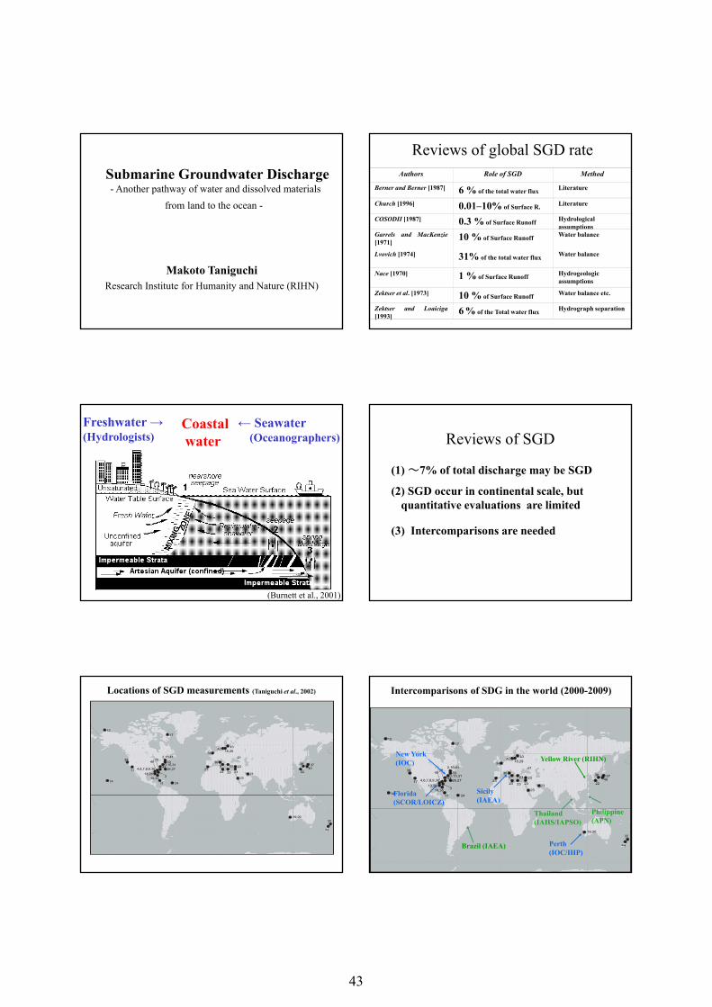
Locations of SGD measurements (Taniguchi et al., 2002)
Reviews of global SGD rateAuthors Role of SGD Method
Berner and Berner [1987] 6 % of the total water flux Literature
Church [1996] 0.01–10% of Surface R. Literature
COSODII [1987] 0.3 % of Surface Runoff Hydrologicalassumptions
Garrels and MacKenzie[1971] 10 % of Surface Runoff Water balance
Lvovich [1974] 31% of the total water flux Water balance
Nace [1970] 1 % of Surface Runoff Hydrogeologicassumptions
Zektser et al. [1973] 10 % of Surface Runoff Water balance etc.
Zektser and Loaiciga[1993] 6 % of the Total water flux Hydrograph separation
Reviews of SGD
(1) ~7% of total discharge may be SGD
(2) SGD occur in continental scale, but quantitative evaluations are limited
(3) Intercomparisons are needed
39
17
17
12
14
4,6,7,8,9,30
45 252,16,41
13,2810,35
331,15,31
43 26,27
3
2411
3442
23
365
23 23 23
2323
2323
21
18,2943
38 3740
22
19,2032
44
Florida(SCOR/LOICZ)
Sicily(IAEA)
Perth(IOC/IHP)
Intercomparisons of SDG in the world (2000-2009)
New York(IOC) Yellow River (RIHN)
Philippine(APN)
Thailand(IAHS/IAPSO)
Brazil (IAEA)
43
2
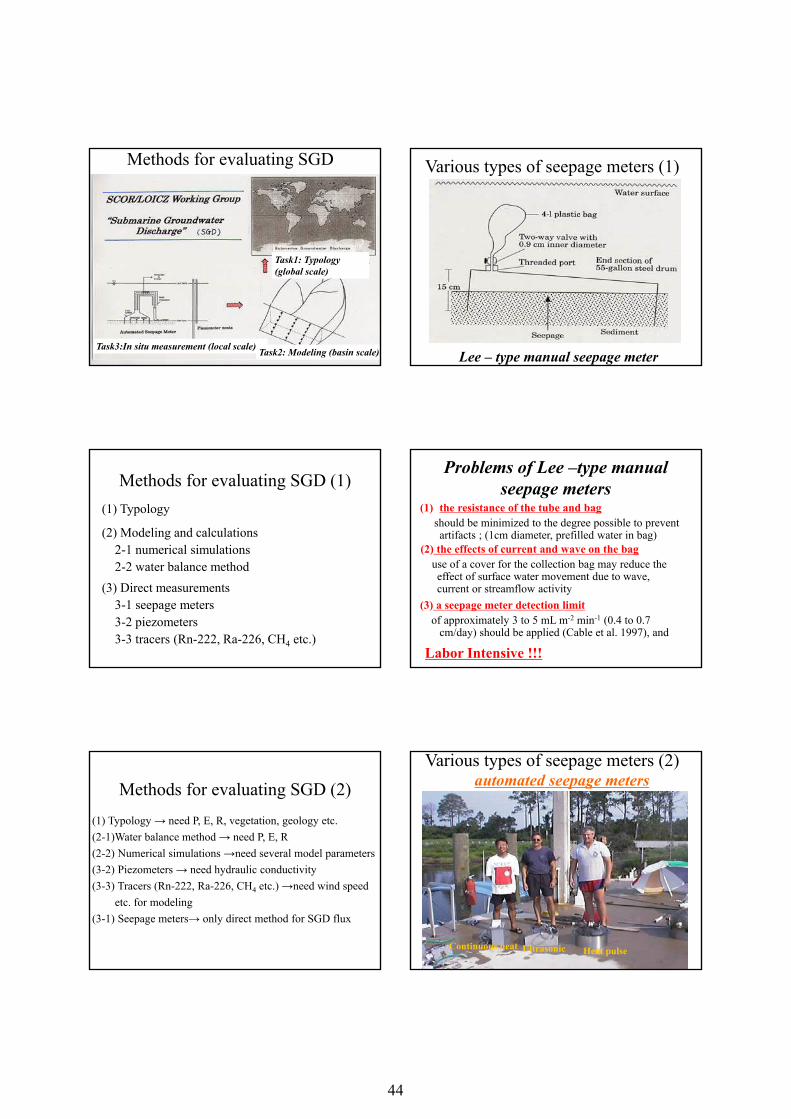
Task3:In situ measurement (local scale)
Task1: Typology (global scale)
Task2: Modeling (basin scale)
Methods for evaluating SGD
Methods for evaluating SGD (1)(1) Typology
(2) Modeling and calculations2-1 numerical simulations2-2 water balance method
(3) Direct measurements 3-1 seepage meters3-2 piezometers3-3 tracers (Rn-222, Ra-226, CH4 etc.)
Methods for evaluating SGD (2)(1) Typology → need P, E, R, vegetation, geology etc.(2-1)Water balance method → need P, E, R(2-2) Numerical simulations →need several model parameters(3-2) Piezometers → need hydraulic conductivity(3-3) Tracers (Rn-222, Ra-226, CH4 etc.) →need wind speed
etc. for modeling (3-1) Seepage meters→ only direct method for SGD flux
Various types of seepage meters (1)
Lee – type manual seepage meter
Problems of Lee –type manual seepage meters
(1) the resistance of the tube and bagshould be minimized to the degree possible to prevent artifacts ; (1cm diameter, prefilled water in bag)
(3) a seepage meter detection limitof approximately 3 to 5 mL m-2 min-1 (0.4 to 0.7
cm/day) should be applied (Cable et al. 1997), and
(2) the effects of current and wave on the baguse of a cover for the collection bag may reduce the effect of surface water movement due to wave, current or streamflow activity
Labor Intensive !!!
automated seepage meters
Continuous heat Ultrasonic Heat pulse
Various types of seepage meters (2)
44
3
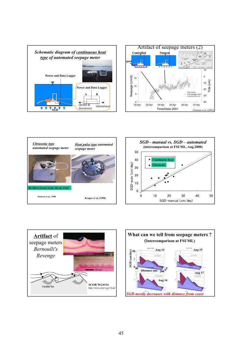
Schematic diagram of continuous heat type of automated seepage meter
A B
Power and Data Logger
SGD
Power and Data Logger
(heater & thermistor)
(thermistor)
Ultrasonic typeautomated seepage meter
Paulsen et al., 1998
Bi-Directional Sonic Beam Path
Heat pulse type automated seepage meter
Kruper et al, (1998)
Artifact of seepage meters
Bernoulli's Revenge
SCOR WG#114http://www.scor-wg114.de/
Artifact of seepage meters (2)
Time/Data 200102-Apr 03-Apr 04-Apr 05-Apr 06-Apr 07-Apr
Seep
age
(cm
/d)
0
5
10
15
20
Tide
(cm
)
-40
-30
-20
-10
0
10
Pool controlAuto seepage meterLong Key tide (cm)
Chanton et al. (2002)
Controlled Natural
pool
0
10
20
30
40
50
0 10 20 30 40 50
SGD-manual (cm/day)
SG
D-au
to (
cm
/da
y)
continuous heat
ul
SGD - manual vs. SGD – automated(intercomparison at FSUML, Aug.2000)
Ultrasonic
Continuous heat
What can we tell from seepage meters ?(Intercomparison at FSUML)
4273
101134
168201
X-transect
Y-transect0
10
20
30
40
50
cm/d
ay
Distance (m)
August 14, 2000
X�¦�= 18.2 L/min.mY-¦ = 18.9 L/min.m
Q = 1.9 m3/min
4273
101134
168201
X-transect
Y-transect0
10
20
30
40
50
cm/d
ay
Distance (m)
August 15, 2000
X�¦�= 13.2 L/min.mY-¦ = 19.7 L/min.m
Q = 1.6 m3/min
4273
101134
168201
X-transect
Y-transect0
10
20
30
40
50
cm/d
ay
Distance (m)
August 16, 2000
X�¦�= 21.7 L/min.mY-¦ = 23.6 L/min.m
Q = 2.3 m3/min
4273
101134
168201
X-transect
Y-transect0
10
20
30
40
50
cm/d
ay
Distance (m)
August 17, 2000
X�¦�= 23.0 L/min.mY-¦ = 26.1 L/min.m
Q =2.53
SGD mostly decreases with distance from coast
50
0SGD
(cm
/day
)
Distance (m) 20040 XY
Aug 14
Aug 16
Aug 17
Aug 15
45
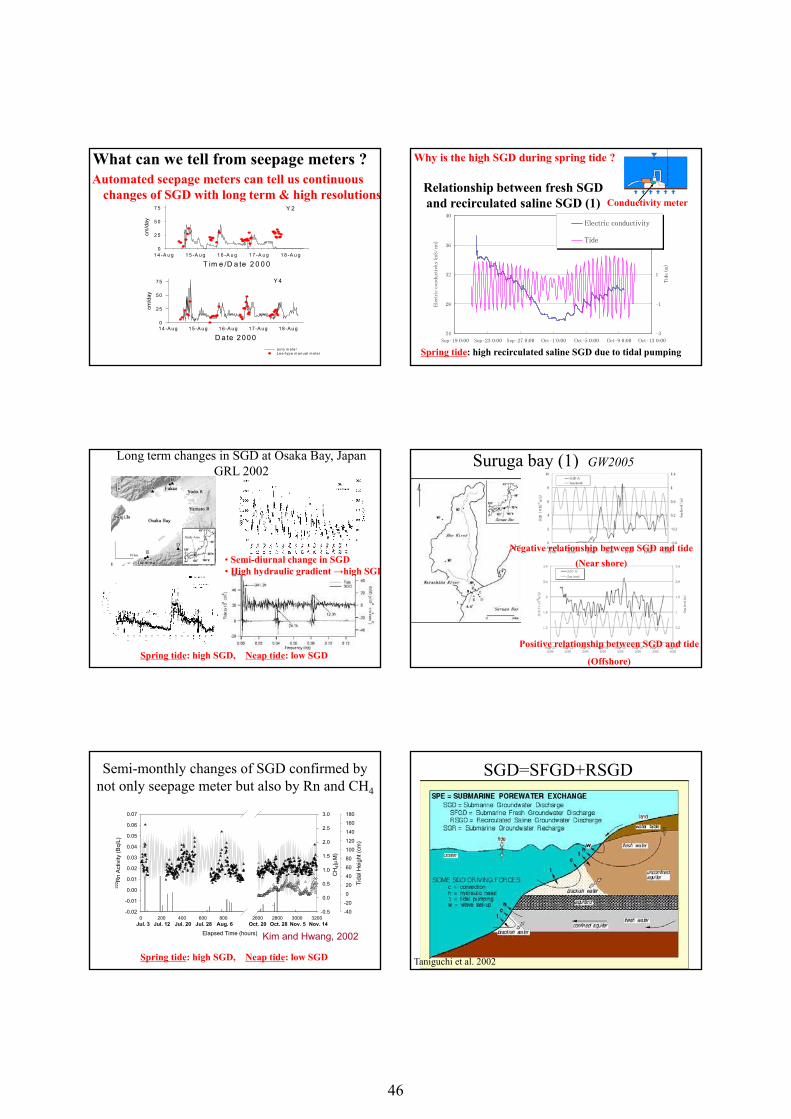
4
What can we tell from seepage meters ?
T im e /D a te 2 0 0 01 4 -A u g 1 5 -A u g 1 6 -A u g 1 7 -A u g 1 8 -A u g
cm/d
ay
0
2 5
5 0
7 5
a u to m e te r L e e - ty p e m e te r
Y 2
D a te 20001 4-A ug 1 5-A ug 1 6-A ug 17-A ug 18-A u g
cm/d
ay
0
25
50
75
au to m e te rLe e-typ e m a nu a l m ete r
Y 4
Automated seepage meters can tell us continuous changes of SGD with long term & high resolutions
Spring tide: high SGD, Neap tide: low SGD
• Semi-diurnal change in SGD• High hydraulic gradient →high SGD
Long term changes in SGD at Osaka Bay, JapanGRL 2002
Semi-monthly changes of SGD confirmed by not only seepage meter but also by Rn and CH4
Elapsed Time (hours)
0 200 400 600 800 2600 2800 3000 3200
Tida
l Hei
ght (
cm)
-40-20020406080100120140160180
222 R
n Ac
tivity
(Bq/
L)
-0.02
-0.01
0.00
0.01
0.02
0.03
0.04
0.05
0.06
0.07
CH
4(P M
)
-0.5
0.0
0.5
1.0
1.5
2.0
2.5
3.0
Jul. 3 Jul. 12 Jul. 20 Jul. 28 Aug. 6 Oct. 20 Nov. 14Nov. 5Oct. 28
Kim and Hwang, 2002
Spring tide: high SGD, Neap tide: low SGD
Relationship between fresh SGD and recirculated saline SGD (1)
24
28
32
36
40
Sep-19 0:00 Sep-23 0:00 Sep-27 0:00 Oct-1 0:00 Oct-5 0:00 Oct-9 0:00 Oct-13 0:00
Ele
ctri
c co
nduct
ivit
y (m
S/cm
)
-3
-1
1
3
5
Tid
e (m
)
Electric conductivity
Tide
Spring tide: high recirculated saline SGD due to tidal pumping
Conductivity meter
Why is the high SGD during spring tide ?
Suruga bay (1) GW2005
Positive relationship between SGD and tide
(Offshore)
Negative relationship between SGD and tide (Near shore)
SGD=SFGD+RSGD
Taniguchi et al. 2002
46
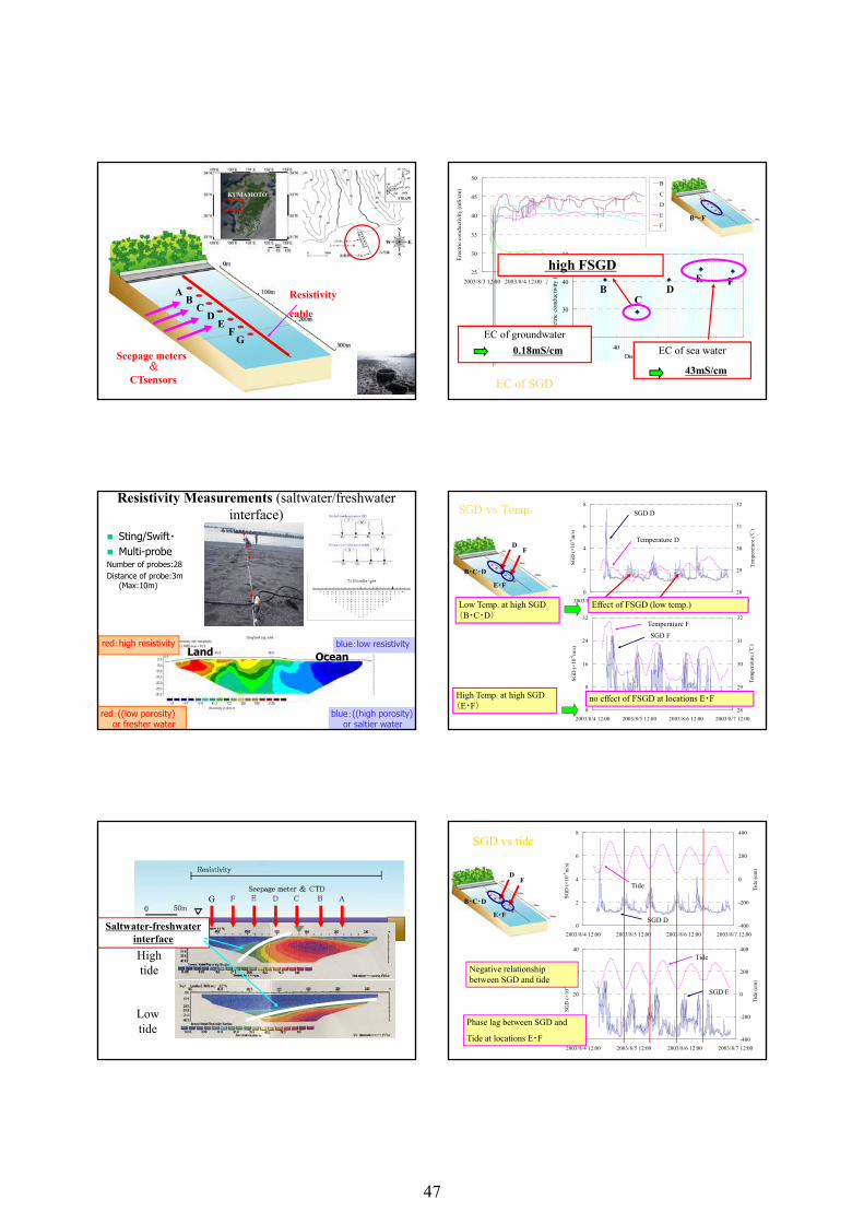
5
AB
CD
EF
G
Resistivity
cable
Seepage meters&
CTsensors
KUMAMOTO
Resistivity Measurements (saltwater/freshwater interface)
� Sting/Swift・� Multi-probeNumber of probes:28Distance of probe:3m
(Max:10m)
red:high resistivity
red:((low porosity) or fresher water
blue:low resistivity
blue:((high porosity) or saltier water
Land Ocean
Low tide
High tide
Resistivityblue: sea water, red: fresh water
Saltwater-freshwater interface
G
EC of SGD
25
30
35
40
45
50
2003/8/3 12:00 2003/8/4 12:00 2003/8/5 12:00 2003/8/6 12:00 2003/8/7 12:00
Erec
tric
cond
uctiv
ity (m
S/cm
)
B
C
D
E
F
20
30
40
50
0 40 80 120 160Distance from the land (m)
Erec
tric
cond
uctiv
ity (m
S/cm
)
BC
DE F
high FSGD
EC of groundwater0.18mS/cm EC of sea water
43mS/cm
B~F
SGD vs Temp.
0
2
4
6
8
2003/8/4 12:00 2003/8/5 12:00 2003/8/6 12:00 2003/8/7 12:00
SGD
(×10
-6m
/s)
28
29
30
31
32
Tem
pere
ture
(℃)
0
8
16
24
32
2003/8/4 12:00 2003/8/5 12:00 2003/8/6 12:00 2003/8/7 12:00
SGD
(×10
-6m
/s)
28
29
30
31
32
Tem
pera
ture
(℃)
Low Temp. at high SGD(B・C・D)
High Temp. at high SGD(E・F)
no effect of FSGD at locations E・F
SGD D
Temperature D
Temperature FSGD F
Effect of FSGD (low temp.)
DF
B・C・D
E・F
SGD vs tide
0
2
4
6
8
2003/8/4 12:00 2003/8/5 12:00 2003/8/6 12:00 2003/8/7 12:00
SGD
(×10
-6m
/s)
-400
-200
0
200
400
Tide
(cm
)
0
10
20
30
40
2003/8/4 12:00 2003/8/5 12:00 2003/8/6 12:00 2003/8/7 12:00
SGD
(×10
-6m
/s)
-400
-200
0
200
400
Tide
(cm
)
SGD D
Tide
Tide
SGD F
Negative relationship between SGD and tide
Phase lag between SGD and
Tide at locations E・F
DF
B・C・D
E・F
47
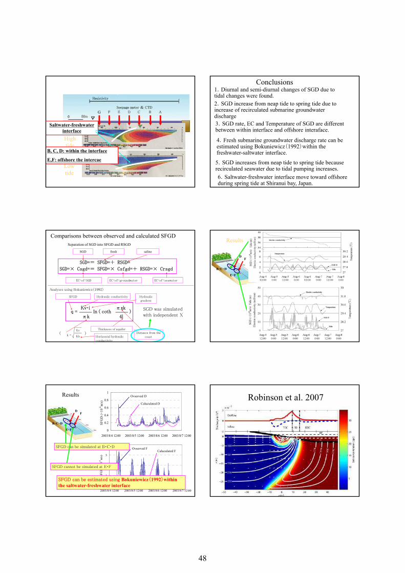
6
Low tide
High tide
Resistivityblue: sea water, red: fresh water
Saltwater-freshwater interface
G
B, C, D: within the interface
E,F: offshore the intercae
Separation of SGD into SFGD and RSGD
SGD = SFGD + RSGD
SGD × Csgd = SFGD × Csfgd + RSGD × Crsgd
SGD salinefresh
EC of SGD EC of groundwater EC of seawater
Analyses using Bokuniewicz(1992)
SFGD Hydraulic gradient
Hydraulic conductivity
k = Kv
Kh( )
Thickness of aquiferDistance from the
coastHorizontal hydraulic conductivity
SGD was simulated with independent X
q =πxk
In ( cothπk
Kv・i)
4l
Comparisons between observed and calculated SFGD
k =
Kv
Results
0
0.2
0.4
0.6
0.8
1
2003/8/4 12:00 2003/8/5 12:00 2003/8/6 12:00 2003/8/7 12:00
SFG
D (×
10-6
m/s)
0
1
2
3
4
2003/8/4 12:00 2003/8/5 12:00 2003/8/6 12:00 2003/8/7 12:00
SFG
D (×
10-6
m/s)
DF
Ovserved D
Caluculated D
Ovserved FCaluculated F
SFGD can be simulated at B・C・D
SFGD cannot be simulated at E・F
SFGD can be estimated using Bokuniewicz(1992)within the saltwater-freshwater interface
B・C・D
E・F
Conclusions 1.Diurnal and semi-diurnal changes of SGD due to tidal changes were found.2.SGD increase from neap tide to spring tide due to increase of recirculated submarine groundwater discharge3.SGD rate, EC and Temperature of SGD are different between within interface and offshore interaface.
4.Fresh submarine groundwater discharge rate can be estimated using Bokuniewicz(1992)within the freshwater-saltwater interface.
5.SGD increases from neap tide to spring tide because recirculated seawater due to tidal pumping increases.6.Saltwater-freshwater interface move toward offshore during spring tide at Shiranui bay, Japan.
Results
DF
B・C・D
E・F
Robinson et al. 2007
48
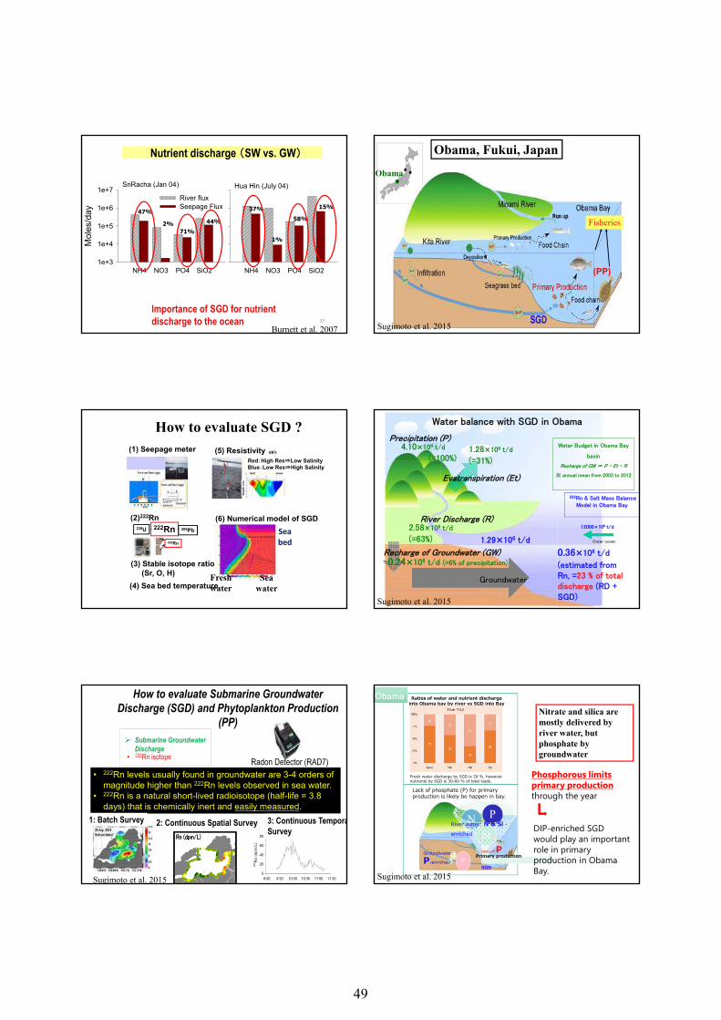
7
37
NH4 NO3 PO4 SiO2
Mol
es/d
ay
1e+3
1e+4
1e+5
1e+6
1e+7River fluxSeepage Flux
NH4 NO3 PO4 SiO2
SriRacha (Jan 04) Hua Hin (July 04)
Nutrient discharge (SW vs. GW)
2%71%
44%
37%
1%
58%
15%47%
Importance of SGD for nutrient discharge to the ocean
Burnett et al. 2007
(1) Seepage meter
238U 222Rn 206Pb→ →
(5) Resistivity Red:High Res⇒Low SalinityBlue:Low Res⇒High Salinity
(2)222Rn
(3) Stable isotope ratio (Sr, O, H)
(4) Sea bed temperature
222Rn
Sea water
Sea bed
(6) Numerical model of SGD
Fresh water
How to evaluate SGD ?
How to evaluate Submarine Groundwater Discharge (SGD) and Phytoplankton Production
(PP)¾ Submarine Groundwater
Discharge• 222Rn isotope Radon Detector (RAD7)
• 222Rn levels usually found in groundwater are 3-4 orders of magnitude higher than 222Rn levels observed in sea water.
• 222Rn is a natural short-lived radioisotope (half-life = 3.8 days) that is chemically inert and easily measured.
1: Batch Survey
9:00 9:30 10:00 10:30 11:00 11:30
222 R
n (d
pm/L
)
0
20
40
60
80
3: Continuous TemporaSurvey
Rn (dpm/L)Rn (dpm/L)
2: Continuous Spatial Survey
Sugimoto et al. 2015
Fisheries
(PP)
Obama, Fukui, JapanObama
Sugimoto et al. 2015
Water balance with SGD in Obama
Water Budget in Obama Bay
basin
Recharge of GW = P – Et - R
※ annual mean from 2003 to 2012
0.36×10⁶ t/d
(estimated from Rn, =23 % of total discharge (RD + SGD)
222Rn & Salt Mass Balance Model in Obama Bay
12000×106 t/d
Outer ocean
Groundwater
2.58×10⁶ t/d
(=63%)
4.10×10⁶ t/d
(=100%)1.28×10⁶ t/d
(=31%)
Evatranspiration (Et)
0.24×10⁶ t/d (=6% of precipitation)
Recharge of Groundwater (GW)
River Discharge (R)
Precipitation (P)
1.29×10⁶ t/d
Sugimoto et al. 2015
SiN P
PSi
SGD
N
River water: N & Si -enriched
Groundwater:
P-enriched
Lack of phosphate (P) for primary production is likely be happen in bay.
lack of PPrimary production
Ratios of water and nutrient discharge into Obama bay by river vs SGD into Bay
(※10 times average)
Fresh water discharge by SGD is 20 %, however nutrients by SGD is 30-60 % of total loads.
Nitrate and silica are mostly delivered by river water, but phosphate by groundwater
Phosphorous limits primary productionthrough the year
DIP-enriched SGD would play an important role in primary production in Obama Bay.
ObamaObama
Sugimoto et al. 2015
49
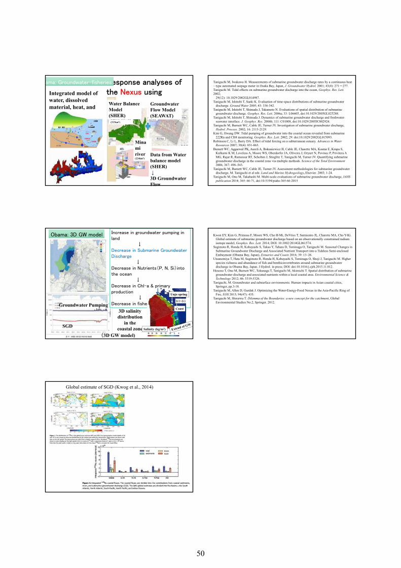
8
Response analyses of the Nexus using integrated model
Integrated model of water, dissolved material, heat, and primary production
ama: Groundwater-fisheriesama: Groundwater-fisheries
Kita river(213km2)
Minami river(224km2)
Water Balance Model (SHER)
Groundwater Flow Model (SEAWAT)
Data from Water balance model (SHER)↓
3D Groundwater Flow
Groundwater Pumping
SGD
Obama: 3D GW modelObama: 3D GW model
3D salinity distribution
in the coastal zone
(3D GW model)
Increase in groundwater pumping in land
↓Decrease in Submarine Groundwater Discharge
↓Decrease in Nutrients(P, N, Si)into the ocean
↓Decrease in Chl-a & primary production
↓Decrease in fisheries
Coast
Salinity (kg/m3)
Unjo spring
Global estimate of SGD (Kwog et al., 2014)
Taniguchi M, Iwakawa H. Measurements of submarine groundwater discharge rates by a continuous heat – type automated seepage meter in Osaka Bay, Japan, J. Groundwater Hydrol. 2001; 43(4): 271-277.Taniguchi M. Tidal effects on submarine groundwater discharge into the ocean, Geophys. Res. Lett. 2002;
29(12): 10.1029/2002GL014987.Taniguchi M, Ishitobi T, Saeki K. Evaluation of time-space distributions of submarine groundwater
discharge. Ground Water 2005; 43: 336-342.Taniguchi M, Ishitobi T, Shimada J, Takamoto N. Evaluations of spatial distribution of submarine
groundwater discharge. Geophys. Res. Lett. 2006a; 33: L06605, doi:10.1029/2005GL025288.Taniguchi M, Ishitobi T, Shimada J. Dynamics of submarine groundwater discharge and freshwater-
seawater interface. J. Geophys. Res. 2006b; 111: C01008, doi:10.1029/2005JC002924.Taniguchi M, Burnett WC, Cable JE, Turner JV. Investigation of submarine groundwater discharge,
Hydrol. Process. 2002; 16: 2115-2129.Kim G, Hwang DW. Tidal pumping of groundwater into the coastal ocean revealed from submarine
222Rn and CH4 monitoring. Geophys. Res. Lett. 2002; 29: doi:10.1029/2002GL015093.Robinson C, Li L, Barry DA. Effect of tidal forcing on a subterranean estuary. Advances in Water
Resources 2007; 30(4): 851-865.Burnett WC, Aggarwal PK, Aureli A, Bokuniewicz H, Cable JE, Charette MA, Kontar E, Krupa S,
Kulkarni K M, Loveless A, Moore WS, Oberdorfer JA, Oliveira J, Ozyurt N, Povinec P, Privitera A MG, Rajar R, Ramessur RT, Scholten J, Stieglitz T, Taniguchi M, Turner JV. Quantifying submarine groundwater discharge in the coastal zone via multiple methods. Science of the Total Environment2006; 367: 498–543.
Taniguchi M, Burnett WC, Cable JE, Turner JV. Assessment methodologies for submarine groundwater discharge, M. Taniguchi et al eds: Land and Marine Hydrogeology, Elsevier. 2003; 1-24.
Taniguchi M, Ono M, Takahashi M. Multi-scale evaluations of submarine groundwater discharge, IAHS publication 2014; 365: 66-71, doi:10.5194/piahs-365-66-2015
Kwon EY, Kim G, Primeau F, Moore WS, Cho H-Mi, DeVries T, Sarmiento JL, Charette MA, Cho Y-Ki. Global estimate of submarine groundwater discharge based on an observationally constrained radium isotope model, Geophys. Res. Lett. 2014; DOI: 10.1002/2014GL061574.
Sugimoto R, Honda H, Kobayashi S, Takao Y, Tahara D, Tominaga O, Taniguchi M. Seasonal Changes in Submarine Groundwater Discharge and Associated Nutrient Transport into a Tideless Semi-enclosed Embayment (Obama Bay, Japan), Estuaries and Coasts 2016; 39: 13–26.
Utsunomiya T, Hata M, Sugimoto R, Honda H, Kobayashi S, Tominaga O, Shoji J, Taniguchi M. Higher species richness and abundance of fish and benthicinvertebrates around submarine groundwater discharge in Obama Bay, Japan. J Hydrol. in press; DOI: doi:10.1016/j.ejrh.2015.11.012.
Hosono T, Ono M, Burnett WC, Tokunaga T, Taniguchi M, Akimichi T. Spatial distribution of submarine groundwater discharge and associated nutrients within a local coastal area. Environmental Science & Technology 2012; 46: 5319-5326.
Taniguchi, M. Groundwater and subsurface environments: Human impacts in Asian coastal cities, Springer, pp.3-18.
Taniguchi M, Allen D, Gurdak J. Optimizing the Water-Energy-Food Nexus in the Asia-Pacific Ring of Fire, EOS 2013; 94(47): 435.
Taniguchi M, Shiraiwa T. Dilemma of the Boundaries: a new concept for the catchment, Global Environmental Studies No.2, Springer. 2012.
50
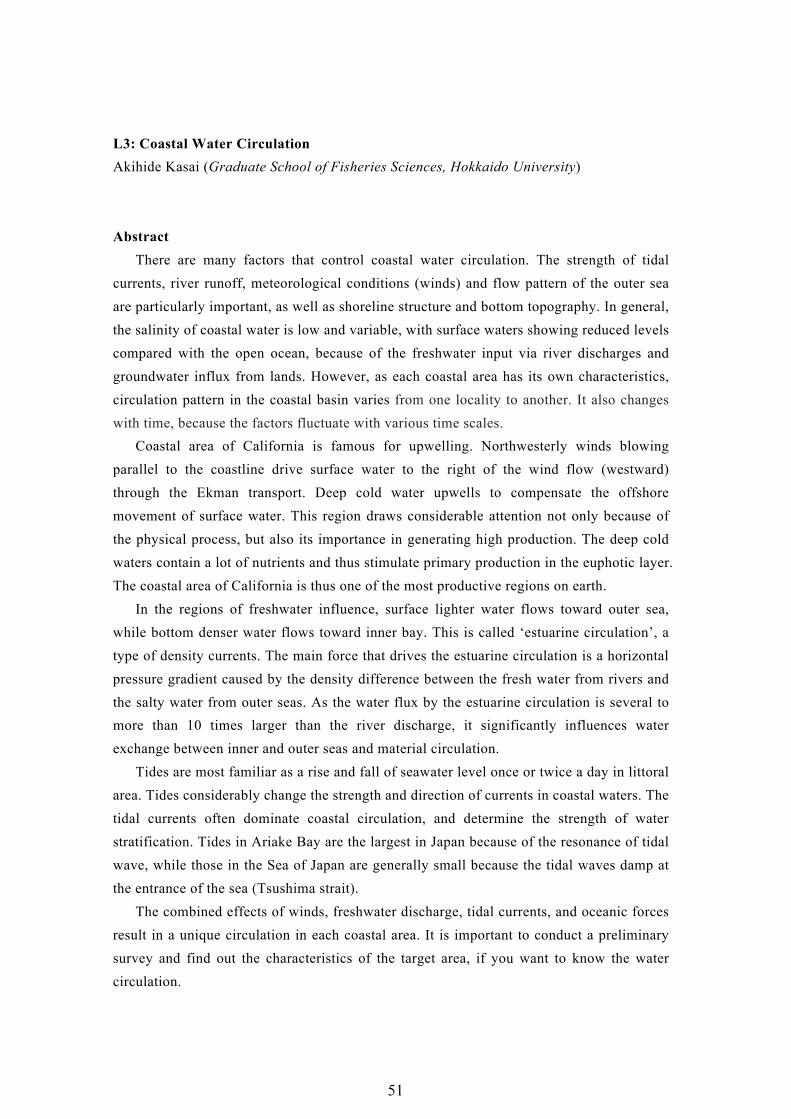
L3: Coastal Water Circulation Akihide Kasai (Graduate School of Fisheries Sciences, Hokkaido University) Abstract
There are many factors that control coastal water circulation. The strength of tidal currents, river runoff, meteorological conditions (winds) and flow pattern of the outer sea are particularly important, as well as shoreline structure and bottom topography. In general, the salinity of coastal water is low and variable, with surface waters showing reduced levels compared with the open ocean, because of the freshwater input via river discharges and groundwater influx from lands. However, as each coastal area has its own characteristics, circulation pattern in the coastal basin varies from one locality to another. It also changes with time, because the factors fluctuate with various time scales.
Coastal area of California is famous for upwelling. Northwesterly winds blowing parallel to the coastline drive surface water to the right of the wind flow (westward) through the Ekman transport. Deep cold water upwells to compensate the offshore movement of surface water. This region draws considerable attention not only because of the physical process, but also its importance in generating high production. The deep cold waters contain a lot of nutrients and thus stimulate primary production in the euphotic layer. The coastal area of California is thus one of the most productive regions on earth.
In the regions of freshwater influence, surface lighter water flows toward outer sea, while bottom denser water flows toward inner bay. This is called ‘estuarine circulation’, a type of density currents. The main force that drives the estuarine circulation is a horizontal pressure gradient caused by the density difference between the fresh water from rivers and the salty water from outer seas. As the water flux by the estuarine circulation is several to more than 10 times larger than the river discharge, it significantly influences water exchange between inner and outer seas and material circulation.
Tides are most familiar as a rise and fall of seawater level once or twice a day in littoral area. Tides considerably change the strength and direction of currents in coastal waters. The tidal currents often dominate coastal circulation, and determine the strength of water stratification. Tides in Ariake Bay are the largest in Japan because of the resonance of tidal wave, while those in the Sea of Japan are generally small because the tidal waves damp at the entrance of the sea (Tsushima strait).
The combined effects of winds, freshwater discharge, tidal currents, and oceanic forces result in a unique circulation in each coastal area. It is important to conduct a preliminary survey and find out the characteristics of the target area, if you want to know the water circulation.
51

52
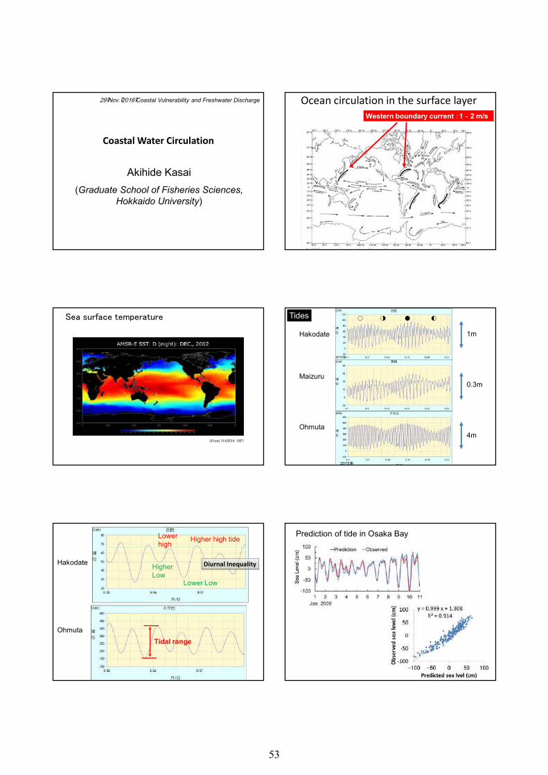
1
Coastal Water Circulation
Akihide Kasai (Graduate School of Fisheries Sciences,
Hokkaido University)
29 Nov. 2016 Coastal Vulnerability and Freshwater Discharge
Western boundary current :1‐2 m/s
Ocean circulation in the surface layer
Sea surface temperature
(From NASDA HP)
30 (oC)0 10 20
Hakodate
Maizuru
Ohmuta
1m
0.3m
4m
🌕 🌗 🌑 🌓
2015年
2015年
Tides
Hakodate
OhmutaTidal range
Higher high tideLower high
Higher Low
Lower Low
Diurnal Inequality
Prediction of tide in Osaka Bay
53
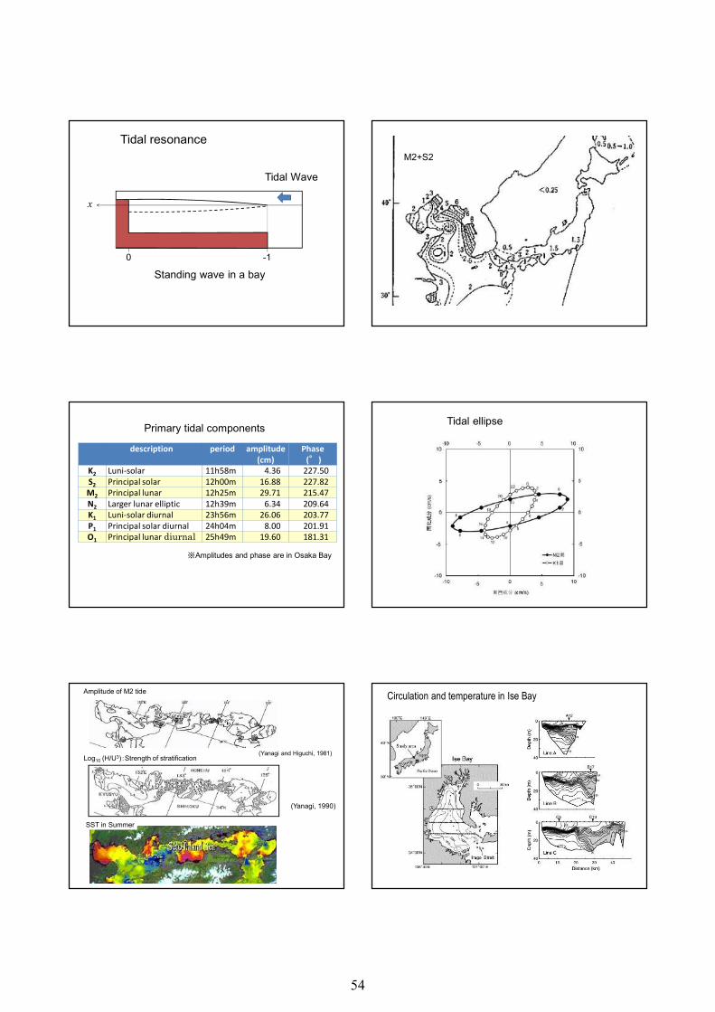
2
Tidal resonance
x
Tidal Wave
Standing wave in a bay0 -1
M2+S2
description period amplitude(cm)
Phase(°)
K2 Luni-solar 11h58m 4.36 227.50S2 Principal solar 12h00m 16.88 227.82M2 Principal lunar 12h25m 29.71 215.47N2 Larger lunar elliptic 12h39m 6.34 209.64K1 Luni-solar diurnal 23h56m 26.06 203.77P1 Principal solar diurnal 24h04m 8.00 201.91O1 Principal lunar diurnal 25h49m 19.60 181.31
Primary tidal components
※Amplitudes and phase are in Osaka Bay
Tidal ellipse
(Yanagi, 1990)
(Yanagi and Higuchi, 1981)
Amplitude of M2 tide
Log10 (H/U3):Strength of stratification
SST in Summer
水温
Circulation and temperature in Ise Bay
54
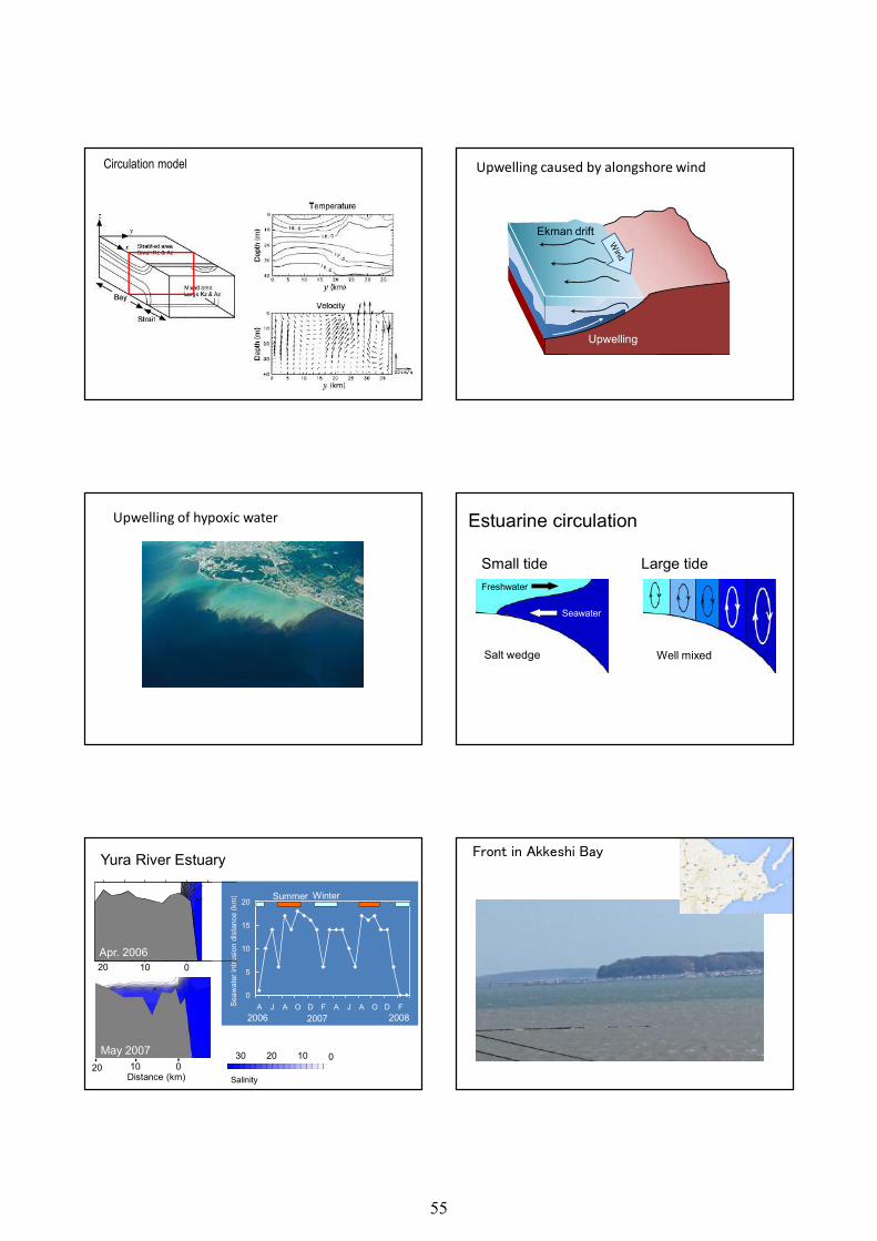
3
Circulation model Upwelling caused by alongshore wind
Upwelling
Ekman drift
Upwelling of hypoxic water
Freshwater
Seawater
Salt wedge Well mixed
Small tide Large tide
Estuarine circulation
0102030
0
5
10
15
20
A J A O D F A J A O D FSeaw
ater
intru
sion
dis
tanc
e (k
m)
2006 2007 2008
Summer Winter
Yura River Estuary
Apr. 200601020
010Distance (km)
May 200720
Salinity
Front in Akkeshi Bay
55

56
L4: Nutrient Dynamics Yu Umezawa (Graduate School of Fisheries and Environmental Sciences, Nagasaki University) Abstract
Understanding nutrient dynamics (i.e., nutrient concentration of each species, distribution, source, and movement etc.) in aquatic ecosystem are indispensable, when we study about phytoplankton species composition, primary production, and environmental problems such as red tide and green tide at coastal areas and lakes. In the oligotorphic waters at pelagic ocean and coral reefs, nutrients are tightly recycled in the ecosystems. Then, remineralization from particulate and dissolved organic matter (POM, DOM) is also important nutrient sources, as well as nitrogen supply through nitrogen fixation. Some species of phytoplankton have higher ability to uptake DOM for their growth. Therefore, POM and DOM are also categorized into nutrients in a broad sense, although component of nutrients are generally nitrate (NO3
-), nitrite (NO2-), ammonium (NH4
+), phosphate (PO43-)
and silicate (SiO44-) in a narrow sense. The analytical protocol of POM and DOM are
briefly lectured in this lecture. In the coastal areas and marginal seas, main nutrient sources are terrestrial water
including groundwater, atmospheric depositions, upwelling waters and currents from adjacent areas. To identify the source of nutrients, stable isotopes techniques are often effectively used as well as other physical parameters (e.g., salinity and temperature), when stable isotopes values of nutrients from each source are distinctively different. Nutrient dynamics based on stable isotopes are introduced with examples of studies at groundwater in Asian mega cities, East China Sea, and Coral Reefs.
Stable isotopes techniques are also applicable to check actual uptake of each source of
nutrients by the primary producers. For example, chemical compositions in macroalgal tissue record time-averaged information of water quality at the exact locations during algal growing period, because most of macroalgae are growing at exact locations, and uptake nutrients only from water column. Therefore, stable nitrogen isotope (δ15N) and nitrogen contents (%) in macroalgal tissue are effectively used to trace nutrient sources for the primary producers at shallow coastal areas. Transplanting experiments using macroalgae and bivalves in cages and associated shift of chemical composition in their tissue are also introduced in this lecture as an effective tool to check spatial variation in nutrient dynamics.
57

58
Nutrient Dynamics Nutrient Dynamics
Yu Yu UmezawaUmezawa((Marine Biogeochemistry Lab. Faculty of Fisheries)Marine Biogeochemistry Lab. Faculty of Fisheries)
International Hydrological International Hydrological ProgrammeProgrammeCoastal Vulnerability and Freshwater DischargeCoastal Vulnerability and Freshwater Discharge
The Twenty six IHP Training CourseThe Twenty six IHP Training Course
Atmospheric Transportation
River water
Air Pollution
Nutrients Flowat Coastal Areas
Groundwater
River water
SGD
Pollution in Freshwater
Ecosystem Degradation Nutrient
Dynamics
Reconstruction of pollution history
カイアシ類カイアシ類繊毛虫類繊毛虫類
従属栄養従属栄養鞭毛虫類鞭毛虫類
Ciliates CopepodsHeterotrophicflagellates
POMPOM
C, N, P flow through the food web dynamics
DINDIN DIPDIP
植物プランクトン植物プランクトンPhytoplankton
SiOSiO4444--
DOCDOC DONDON
従属栄養従属栄養バクテリアバクテリア
HeterotrophicBacteria
DOPDOP
Microbial LoopMicrobial Loop
Trace MetalsTrace MetalsVitaminsVitamins
River & Groundwater,River & Groundwater,Atmosphere, Sediment, UpwellingAtmosphere, Sediment, Upwelling
Representative Nitrogen Compounds in SeawaterRepresentative Nitrogen Compounds in Seawater
(Dissolved Matter: < 0.2 ~ 0.7 μM)
(Particulate Matter: > 0.2 ~ 0.7 μM )
(Dissolved Inorganic Nitrogen)…. Nitrate, Nitrite, Ammonium ( NO3- NO2- NH4+)
(Dissolved Organic Nitrogen)…. (Amino acids、Urea、Amino sugars etc. )
DIN
DON
N2
Gaseous molecule
( μ )
(Nonreactive・Stable)….(Reactive・Unstable)…. (NO, NO2, N2O etc.)
(Particulate Organic Nitrogen)….(Particulate Inorganic Nitrogen)….
(Organism、Detritus、etc. )
(Mineral、etc. )
PIN
PON
TerrestrialTerrestrial PONPON
DINDIN
Amino acidAmino acidProtein for Protein for PhotosynthesisPhotosynthesis
NHNH44++
NN22DONDONDINDINDONDON
AtmosphericAtmospheric
AssimilationAssimilationDecompositionDecomposition
AdvectionAdvectionNONO33
--
DONDON
Nitrogen (N) Cycle Nitrogen (N) Cycle
PON/DONPON/DON
NONO33--NHNH44
++
NONO33--
NN22OONN22
UpwellingUpwellingSinkingSinking MixingMixing
NitrificationNitrification DenitrificationDenitrification
DecompositionDecomposition
DONDON
DiffusionDiffusion
DiffusionDiffusion
OrthophosphatePyrophosphate (diphosphoric acid)
Polyphosphate
O=P-(OH)3
O=P-(OH)2
O=P-(OH)2
-O-
O=P-O(O-1) n
(SRP)
Apatite, Clay, Oxyhydroxides
> 90%
Representative Phosphorus Compounds in SeawaterRepresentative Phosphorus Compounds in Seawater
DIPDIP
(Dissolved Matter: < 0.2 ~ 0.7 μM)
Orthophosphate monoester・・・Intermediate metabolite during biosynthesis
Orthophosphate diester・・・Phosphodiester bond in phospholipids, ATP・DNA・RNA
Phosphonate
DOP
(Particulate Inorganic Phosphorus)…. (Organism、Detritus、etc. )
(Mineral、etc. )PIPPOP (Particulate Organic Phosphorus)….
(Particulate Matter: > 0.2 ~ 0.7 μM )
59
POPPOPDIPDIP
ATP/ADP/AMP膜リン脂質(PL)DNA/RNA糖リン酸 フィチン酸
PO43-
O – P –OO
O
––
APase
DOPDOPTerrestrialTerrestrial
AssimilationAssimilation
HydrolysisHydrolysis
AdvectionAdvection
DOPDOPDIPDIP
AtmosphericAtmospheric POPPOP
??
Phosphorus (P) Cycle Phosphorus (P) Cycle
POPPOP
Fe(OOH)PFe(OOH)P
DIPDIP
糖リン酸、フィチン酸C-O-PO-PC-P
+ H2O
APase
DOPDOPUpwellingUpwelling
SinkingSinking
DiffusionDiffusionDecompositionDecomposition
HydrolysisHydrolysis
DiffusionDiffusion
MixingMixing
Coloring reaction of nitriteColoring reaction of nitrite
Azo compoundSulfanilamide
Diazo compoundN-1-Naphthylethylenediamine Dihydrochloride
Concentration is calculated based on the intensity of colorConcentration is calculated based on the intensity of color
PhosphatePhosphate MolybdateMolybdate Molybdenum complex Molybdenum complex ((Mo(IV)Mo(IV)))
Reduction by Reduction by
Acidic conditionAcidic condition
Coloring reaction of phosphateColoring reaction of phosphate
ascorbic acidascorbic acid
Concentration is calculated based on the intensity of colorConcentration is calculated based on the intensity of color
Molybdenum complex Molybdenum complex ((Mo(V)Mo(V)))
Nutrients are analyzed by colorimetric method
Lamp Detection
Absorbance
sa
Patey et al. (2008) TRACS
Reagent 1
Reagent 2
Air
Sample
Ready-made commercial product
Hand-made assembling product
Detection limit (0.05-0.1 μM)
Detection limit (0.005-0.01 μM)
General Nut. Anal. Nanomolar Nut. Anal.c.a. 80,000 US $ for 2 ch. c.a. 30,000 US $ for 2 ch.
Stable, automated Flexible,
On board continuous analyses of nanomolar nutrients in surface water expanded the understanding of nutrient dynamics in pelagic water
HashihamaHashihama et al. (2009) GRL et al. (2009) GRL
60
Importance of DOM, POM and remineralized nutrients
Remineralized nutrients through the decomposition of POM and DOM support primary production at
ologotrophic waters.
Average composition of nitrogen pools (except dissolved N2)In open ocean (surface & deep), coastal & estuarine waters
Berman & Berman & BronkBronk (2003) MEPS (2003) MEPS
TOPTOP
POPO44 (DIP)(DIP)
CC
DD
A B C DA B C D
P P ((μ
MμM))
60 N60 N
50 N50 N
40 N40 N
30 N30 N
North Pacific subtropical gyre
海洋に存在する溶存態窒素の存在形態の場所別比較
DON pool dominates the surface ocean fixed N reservoir, comprising up to 96-99% of (TDN) in the oligotrophic ocean
AbellAbell et al. (2000) J. Mar Res et al. (2000) J. Mar Res
TONTON
DINDIN
N
N ((μ
MμM))
AA
BB20 N20 N
10 N10 N
00
DON pool dominates the surface ocean fixed N reservoir, comprising up to 96-99% of (TDN) in the oligotrophic ocean
5
10
15
20
25
PONDONDIN
Composition of each form of N and P in the bay
N(μ
M)
NMouth of Bay Mouth of Bay ~~ Inner area of BayInner area of Bay
A1A1A4A4
A6A6
A8A8A9A9
A11A11A13A13
A15A15
0
00.20.40.60.8
11.21.4
POPDOPDIP
P(μM
)
Organic N and P are Organic N and P are dominant formdominant formPOM decrease offshore , POM decrease offshore ,
while DOM are almost while DOM are almost constant throughout the bayconstant throughout the bay
A1 A4 A6 A8 A9 A11 A13 A15
A1 A4 A6 A8 A9 A11 A13 A15
P
((AriakeAriake Sea, Japan, September, 2013)Sea, Japan, September, 2013)
UmezawaUmezawa et al. (2015)et al. (2015)
Identification of POC based on δ13C value
80
100
120Mouth of bay
Innermost area
nc.(μM
)
Chikugo River(n=3)
Middle areaInnermost area
Δδ13C:- 0.1~-0.2 (‰/day)
Δδ15N:- 0.2~-0.5 (‰/day)Umezawa et al. (2014)
Shift of δ13C and δ15N along the decomposition
0
20
40
60
80
-25 -23 -21 -19 -17 -15
POC
con
δ13C (‰)
Typical range of Marine Phytoplankton
Typical range ofriver-derived POM
Mouth of BayMiddle area
POC: PON ratio
≒7.0POC: PON ratio
≒10.0Surface
Middle
Bottom
Ozaki (2016)Ozaki (2016)
OC
(μM
)
OC
(μM
)
DOC: DOP ratioDOC: DON ratio
8060
40100
100Innermost
Mouth of Bay
C/N, C/P ratios increase with distance from the river
InnermostMouth of Bay
DO DO
2 3 4 5 6 7 8 DON (μM)
0.05 0.2 0.5DOP (μM)
20
100.01 0.1 1
101 10
The quality of POM decreases from innermost area to the mouth of bay, in the viewpoint of the source of DIN & DIP
Ozaki (2016)Ozaki (2016)
61
Seawater in SCM layer collected from Seawater in SCM layer collected from innermost areainnermost area, , middle area middle area and and mouth of the mouth of the baybay in in AriakeAriake Sea were incubated in dark, and water quality was monitored .Sea were incubated in dark, and water quality was monitored .
(t=0, 1, 3, 7, 14, 30 days(t=0, 1, 3, 7, 14, 30 days))Dark, in situ temp.
r
A. Decomposition rate of all of organic matter
Incubation Experiments: Nutrients fluxes released through the decomposition of POM and DOM
GF/F (0.7μm)
Seaw
ate
r
B. Decomposition rate of dissolved organic matter
C. Decomposition rate of particulate organic matter
A-B =
Filtration
(200 μm)
Evaluation of Evaluation of remineralizedremineralized nutrientsnutrientsavailable for phytoplankton available for phytoplankton
sed
DIN
sed
DIN
((μMμM
/day
/day
))
Nutrients fluxes released through the decomposition of OM
湾奥
湾央
湾口(橘湾)
(July)
(July)
(September)
Innermost area
Released DIPReleased DIP((μMμM/day/day))
Rele
asRe
leas
((POMPOM::c.a.35c.a.35、、DOM: c.a. 25DOM: c.a. 25--3535))((DIN/PDIN/P::c.a. 10c.a. 10--1515))
・Nutrients release rate are high at the innermost bay area
(September)
(July)(September)
Mouth of bay
Middle area
・NP ratio of released nutrients are low than that of source OM
UmezawaUmezawa et al. (2015)et al. (2015)
Nitrogen Phosphorus0.4
0.3
0 2P/ O
rgan
ic N
, P
7474%%
Labile Organic Matter
BA
C
Spatial variation of DIN, P release rate per OM
The ratio of labile component in the organic matter at the The ratio of labile component in the organic matter at the mouth of bay is 5mouth of bay is 5--10% of that at the innermost area of the bay10% of that at the innermost area of the bay
0.2
0.1
0.0Rele
ased
DIN
P
6060%%
55%%88%%
Umezawa et al. (2015)
RefractoryOrganic Matter
St. A B C St. A B C
Nutrient Dynamics in the East China Sea
Most damaged ecosystem by human activities
Japan Sea(East Sea)
Sea of OkhotskRussia
Mongolia
Huanghe River
Marginal Seas in East Asia
Pacific OceanEast China Sea
( )
South China Sea
Yellow SeaChina Japan
Changjiang River
NagasakiContinental Shelf(< 200 m)
(1/30 of the C.S. in the world)
Geographic characteristics of the ECS~Broad Continental Shelf ~
Okinawa Trough(1500-2000 m)
62
The North Sea
ECS & Surrounding coastal areas
Eastern Caribbean
Halpern et al. (2008) ScienceCumulative human impact in the worldCumulative human impact in the world
How to evaluate vulnerabilityHow to evaluate vulnerability of ecosystem?of ecosystem?負荷要因負荷要因 重み付け重み付け 生態系応答生態系応答
(Ui) (Ej)水温水温
航路航路 砂地砂地
生態系脆弱度生態系脆弱度(I)(I)Human Impact Human Impact CategoriesCategories
(Di)
TemperatureTemperature
S dS d
FactorsFactors WeightingWeighting Response of Ecosystem Response of Ecosystem BiodiversityBiodiversity
Cumulative ImpactsCumulative Impacts積算的な影響積算的な影響
Vulnerability of the ecosystemVulnerability of the ecosystem
漁業漁業
汚濁汚濁
DODO
藻場藻場
岩礁岩礁
積算的な要因積算的な要因 I = ∑ ∑Di*Ej*Ui, jj=1i =1
n m
( 参考: Halpern et al. 2008)
Boat DamageBoat Damage
Over fishingOver fishing
PollutionsPollutions
Sand areaSand area
Rocky shoreRocky shore
SeagrassSeagrass bedbed
Summed DriversSummed Drivers
ECS is important area asECS is important area as hatchery & nurseryhatchery & nursery
Japanese jack mackerel
Japanese anchovy
(Seikai National Fisheries Research Inst. )
1000
2000
3000
4000
5000
6000
400400
350350
6,0006,000
5,0005,000
4,0004,000
3,0003,000
2,0002,000
1,0001,000Fish
Cat
ch (1
000
t)Fi
sh C
atch
(100
0 t)
Decrease of fisheryDecrease of fishery resources at ECSresources at ECS
01
Fish
Cat
ch (1
000
t)Fi
sh C
atch
(100
0 t) 350350
300300
250250
200200
150150
100100
5050
001947 1952 1957 1962 1967 1972 1977 1982 1987 1992 1997 2002 2007 1947 1952 1957 1962 1967 1972 1977 1982 1987 1992 1997 2002 2007
001956 1966 1976 1986 1996 2006 20131956 1966 1976 1986 1996 2006 2013
Chen et al. (1997)
水産庁HP
中国渔业统计年鉴
High NOHigh NO33-- (>25)(>25)
Seasonal change of Seasonal change of NONO33-- distributiondistributionWinterSummer
NE MonsoonNE Monsoon
High POHigh PO4433-- (>1.6)(>1.6)
High SiOHigh SiO2 2 (>30)(>30)
gg 33
Low POLow PO4433-- (<0.05)(<0.05)
Low SiOLow SiO2 2 (<3)(<3)
Low NOLow NO33-- (<0.2)(<0.2)
Low POLow PO4433-- (<0.2)(<0.2)
Low SiOLow SiO2 2 (<5)(<5)
Low NOLow NO33-- (<2.0)(<2.0)
(SCSIW)(SCSIW)
(KW)(KW)
ArthurArthur--Chen (2008) JO Chen (2008) JO
Low NOLow NO33-- (<0.2)(<0.2)
NN--fixing areafixing area
High NOHigh NO33--
River dischargeRiver discharge
UpwellingUpwellingHigh NOHigh NO33
--
SCS Intermediate Water (SCSIW)SCS Intermediate Water (SCSIW)(350 (350 –– 1350 m)1350 m)
KuroshioKuroshio Water (KW)Water (KW)
63
Impact of terrestrial material input from China
Primary production at ECS is highly supported by material fluxes from China.
33Jan. 19-20, 2011 International Symposium on Coastal Resources, Nagasaki
33
Chlorophyll a distribution simulated based on satellite data & model
植物プランクトン植物プランクトン
Phytoplankton
Increase of annual nutrients discharge through CJ River
Wang et al., 2014
N fertilizerCatchment of CJ river
Increase of fertilizer input & discharge excess NEfficiency of fertilizer uptake have decreased with an increase of fertilizer N application
1980X 1990
2000
され
た窒
素量
(t)
Liu et al. (2006) Biogeochemistry
作物
とし
て収
穫さ
施肥された窒素量(t)
G. of MexicoG. of Mexico
Sea of OkhotskSea of Okhotsk
North Sea North Sea Baltic Sea Baltic Sea Kara Sea Kara Sea Laptev Sea Laptev Sea
HadsonHadson BayBay
Gulf of St. LawrenceGulf of St. Lawrence
Jan. 19-20, 2011 International Symposium on Coastal Resources, Nagasaki 36
Black SeaBlack Sea
East China SeaEast China Sea
Bay of BengalBay of Bengal Gulf of ThailandGulf of Thailand
Mediterranean SeaMediterranean Sea
Riverine nutrient fluxes (Gmol/yr) at Major Marginal Seabased on NEWS model (Seitzinger et al., 2005)
Name DIN DIP DON DOP PN PP POCBaltic Sea 19.8 0.68 7.5 0.22 4.7 0.86 49
Bay of Bengal 222.5 3.54 51.8 1.58 99.0 24.37 1396
Black Sea 23.6 1.47 10.5 0.38 8.8 1.75 100
East China Sea 122.7 2.55 25.3 1.03 71.6 13.72 783
Gulf of Mexico 77.2 1.28 17.1 0.54 29.7 5.96 34055Gulf of St. Lawrence 15.7 0.29 17.5 0.47 5.3 0.96 55
Gulf of Thailand 10.4 0.22 6.1 0.17 8.9 1.74 100
Hudson Bay 8.3 0.14 11.8 0.27 6.7 1.21 69
Kara Sea 16.0 0.47 17.1 0.42 18.7 3.51 200
Laptev Sea 3.4 0.09 7.8 0.17 10.6 1.98 113
Northern Adriatic Sea 11.9 0.50 3.3 0.10 4.5 1.06 61
North Sea 58.4 2.44 13.8 0.47 7.4 1.40 80
Sea of Okhotsk 19.9 0.58 8.5 0.21 8.7 1.63 93
DIN: Dissolved Inorganic Nitrogen
DON: Dissolved Organic Nitrogen
DOP: Dissolved Organic PhosphorusPN: Particulate NitrogenDIP: Dissolved Inorganic Phosphorus PP: Particulate PhosphorusPOC: Particulate Organic Carbon
Annual shift of nutrient composition in Yangtze RiverYangtze River Floods Enhance Coastal Ocean Phytoplankton Biomass & Potential Fish Production
(Riverwater Discharge)
(Area affected by Changjiang Diluted water )
(Fixed carbon volumeby phytoplankton)
on F
ixed
(ton
sCd-1
)
char
ge (m
3s-1
)
Gong et al. (2011)
CDW
are
a (k
m2 )
orC
arbo
Rive
r wat
er D
isc
64
Annual variation of Phytoplankton Biomass & Potential Fish Production, due to the different discharge rate.
July 1998 July 2004 July 2007
Gong et al. (2011)
July 2008 July 2009 July 2010
Si / N
conc
. (μM
)
onc.
(μM
)P
ratio
N ra
tio
Si : Silicate
Annual shift of nutrient composition in Changjiang River
DIN:Nitrogen
DIP:PhosphorusN/P
DIN
, Si
DIP
co N/P
Si/N
1960 1970 1980 1990 2000 1960 1970 1980 1990 2000
River-derived N & P loadingsare increasing in the ECS, while Si input is decreasing.
River-derived N loadingsrelatively increase (Higher N/P ratio) Wang et al. (2006) ECS
Shift of N* (= [DIN] – 13x[DIP]) during 10 years
Atmospheric N deposition strengthen N-rich conditionN
Excess
Kim et al. (2011) Science
N depletion
Dinoflagellate
Diatom(Chaetoceros affine )
silicate demandw/ vacuole for nutrients stock
Does nutrient shift change phytoplankton species?
Dinoflagellate( Prorocentrum dentatum)
Coccolithophorid( Emiliania huxleyi.) Mixotrophs
Free swimmingFree swimmingHigher affinity to nutrients Higher affinity to nutrients
Maximum cell density of P. Dentatum in each research cruise
Observed cell density of dinoflagellate is increasing in the ECS
Kiyomoto et al. (2013)(Hokkaido Univ)
P. Dentatum
Eutrophication causes heavy hypoxia in river mouth
Li & Daler (2003) AMBIO
65
Healthy ConditionHealthy ConditionRiver River –– derived nutrients derived nutrients Phytoplankton ProductionPhytoplankton Production
Yangtze River Floods Enhance Coastal Ocean Phytoplankton Biomass & Potential Fish Production
Potential Fish ProductionPotential Fish Production
Excess nutrients inputsExcess nutrients inputsRed tide Red tide
MicroMicro-- & Macro& Macro--algal bloomalgal bloom
×
Changjiang River derived Nutrients Enhance CoastalPhytoplankton Biomass & Potential Fish Production ??
密度躍層
Deteriorated ConditionDeteriorated Condition
PycnoclinePycnocline×DecompositionDecompositionRespirationRespiration
Extra Organic MatterExtra Organic Matter
COCO22 + H+ H22O CHO CH22O + OO + O22
HypoxiaHypoxia ×
密度躍層
Marginal Seas categorized by forcing functionMarginal Seas categorized by forcing functionThermohaline
DeepCon -vection
Ice Form-ation
River Runoff
Wind Tropical Storms
Tides Bound-aryCurrents
External Forcing
55 55 00 00 33 00 11 00 0055 55 00 11 11 00 11 00 0033 00 00 55 33 00 11 00 00
11 00 00 33 11 33 11 55 00
33 33 33 11 33 11 11 33 11
Red SeaRed Sea
Med. SeaMed. Sea
Black SeaBlack Sea
G. of MexicoG. of MexicoJapan SeaJapan Sea
11 00 00 11 11 11 33 33 55
11 00 00 11 33 55 ?? ?? 33
11 00 00 11 33 33 11 33 33
11 00 11 33 55 11 55 00 11
11 00 00 11 33 33 11 55 11
33 33 33 33 33 00 33 11 33
33 33 33 11 33 00 33 00 33
Indonesian SeasIndonesian Seas
South China SeaSouth China Sea
Caribbean SeaCaribbean Sea
Yellow SeaYellow SeaEast China SeaEast China Sea
Sea of OkhotskSea of Okhotsk
Bering SeaBering Sea[ 0 = Not Happening; [ 0 = Not Happening; 11 = Minor Factor; = Minor Factor; 33 = Important; = Important; 55 = Dominant Factor]= Dominant Factor]
Ramp. S.R. (1997) Ramp. S.R. (1997)
Various forcing functions and physical factors influencing nutrient dynamics
http://www.environmentservices.com/projects/programs/RedSeaCD/DATA/definitions.htm
Upwelling occurs by the meander/frontal eddy events
Michel, J. (ed.). 2013.
Changjian River
4.843.85.1
18.822324.5
Box-model input/output of the nutrients at ECS Yellow Sea
黄海
Atmospheric deposition
大気降下物
-0.01-0.3
-0.03
0.11.00.1
0.40.2
0.01
2.10.5
0.01 ECS
夏季 冬季
Burial or export as POM
8.129.710.6
Outflow流出
Changjian River(長江)
Kuroshio Subsurface Water
黒潮亜表層水
Taiwan Current Warm Water台湾暖流水 Zhang et al (2007) Prog Oceanogr
2.029.51.6
14.115317.3
2.927.63.7
6.776.713.1
111
111
SCS
Sediment堆積物 0.4
1.90.6
1.24.21.8
DINDIPDISi
66
Nitrate and ammonium contaminationin the groundwater of Asian megacities
Warm and humid climate condition throughout the year may enhance the bacterial denitrification,
resulting in reduced nitrate contamination.
NitrificationNitrification
[NO[NO33--] ] can be controlled by the can be controlled by the NN source & Redox conditionssource & Redox conditions
NONO33--
OxicOxic conditioncondition
Atmospheric Atmospheric depositionsdepositions
FertilizerFertilizer
(symbols:IAN.umces.edu/)
NONO33
SewageSewageFertilizerFertilizerDenitrificationDenitrificationAnoxic conditionAnoxic condition
NHNH44++
Geological Setting and sampling locationsGeological Setting and sampling locations
ManilaManila BangkokBangkok JakartaJakarta
Shallow GWShallow GW Deep GWDeep GW River WaterRiver Water Spring WaterSpring Water( < 100m )( < 100m ) ( > 100m )( > 100m )
Old flood or tidal plainOld flood or tidal plainVolcanic Volcanic Alluvial FanAlluvial Fan
0 10 20 30 km0 10 20 30 km 0 60 120 180 km0 60 120 180 km 0 45 30 45 km0 45 30 45 km
Volcanic Volcanic Basement rocksBasement rocksSedimentary rocksSedimentary rocks
The relations between The relations between nutrientsnutrients and land useand land use
ManilaManila BangkokBangkok JakartaJakarta
Urban AreaUrban Area Paddy FieldsPaddy Fields
NHNH44++
NHNH44++
NHNH44++
Dry FieldsDry Fields
~ 800 μM WHO standard for drinking water
NONO33--NONO33--
NHNH44++
AmmoniumAmmoniumNitrateNitrate + Nitrite+ Nitrite
Umezawa et al. (2009) STOTEN
Typical ranges of Typical ranges of δδ1515NN・・δδ1818O in NOO in NO33-- from various sourcesfrom various sources
NONO33-- in Precipitationin Precipitation
Fossil Fossil FuelFuelBurningBurningAutomobileAutomobile
ExhaustExhaust
Manure and Septic WasteManure and Septic Waste
NONO33-- FertilizerFertilizer
Nitrification of NHNitrification of NH44++ in fertilizerin fertilizer
Kendall (1998)Kendall (1998)
TaipeiShallow GW
Deep GWRiver waterRain water
BangkokShallow GW
Deep GWRiver water
Severe contribution of sewageSevere contribution of sewage derived NOderived NO33--
Minor contribution of atmospheric NOMinor contribution of atmospheric NO33--
Nitrate δ15N・δ18O values in groundwater and river water
River water
JakartaShallow GW
Deep GWRiver water
Spring water
ManilaShallow GW
Deep GWRiver waterRain water
Active Occurrence of Active Occurrence of denitrificationdenitrification!!
Umezawa et al. (2009) STOTEN
67
Identification of NO3 source in the continental shelf of ECS
The sources of NO3, which were actually incorporated into phytoplankton, are identified
δ δbased on δ15N and δ18O in NO3 in the water column
March, 2012February, 2009
KSW~KSSW~KIWKSW~KSSW~KIW
CDWCDW((ChangjiangChangjiangDiluted water)Diluted water)
YSCWMYSCWM(Yellow(Yellow SeaSea ColdColdWaterWater Mass)Mass)
SMWSMW(Shelf Mixed Water)(Shelf Mixed Water)
(黄海混合水)黄海冷水塊
長江希釈水
July, 2011
CTD, DO, Chl. Fluorescence, CTD, DO, Chl. Fluorescence, Nutrients, POC/N, DOC/N/P, Nutrients, POC/N, DOC/N/P, Chl.Chl.aa
Monitored ParametersMonitored ParametersTWCWTWCW(Taiwan Warm(Taiwan WarmCurrent Water)Current Water)
((KuroshioKuroshio Surface Water)Surface Water)(Shelf Mixed Water)(Shelf Mixed Water)
台湾暖流水
黒潮表層水
黒潮亜表層水
黒潮中層水
大陸棚水
CDWCDW
YSCWMYSCWMδδ1515N = N = 6.5–7.5‰
δδ1818O = O = 5.0–7.0‰
δδ1515N = N = 2.0–8.3‰
δδ1818O =O = 1.9–2.6‰
(黄海混合水)
大陸棚水
黄海冷水塊
長江希釈水
TWCWTWCW
KSWKSWKSSWKSSWKIWKIW
δδ1515N = N = 5.5–6.0‰
δδ1818O = O = 3.5–4.0‰
δδ O O 1.9 2.6‰
δδ1515N = N = ? ‰δδ1818O = O = ? ‰
Liu et al (2010) Env. Sci. TechChen et al. (2013) Acta Ocean Sin
RainwaterRainwater
δδ1515N = N = 0.4±2.9‰
δδ1818O = 73.3O = 73.3±9.8‰
台湾暖流水
黒潮表層水
黒潮亜表層水
黒潮中層水
TWCW
KSSW
SMW
CDW長江希釈水
30
25
20
15TWCWKSSW
YSCWM
CDWSMW
台湾暖流水
大陸棚水
mp
erat
ure
( C
)°
Temperature- Salinity diagram in July, 2011
KIWYSCWM
23.0 29.0 30.0 31.0 32.0 33.0 34.0
July, 2011
15
10
5
TWCW
黄海冷水塊
Developed YSCWM & CDW
~ ~
Salinity
P.T
em
30
25
20
15
10
5
TWCW KSW
KSSW
KIW
SMW
YSMW
CCW
30March, 2012
Feb., 2009 台湾暖流水 黒潮表層水
黒潮亜表層水
黒潮中層水黄海混合水
大陸棚水
中国沿岸水P.T
emp
erat
ure
( C
)°
TWCW KSSW
YSMW
CCW SMW
32.0 32.5 33.0 33.5 34.0 34.5 35.0
32.0 32.5 33.0 33.5 34.0 34.5 35.0
25
20
15
10
5
TWCW KSW
KSSW
KIW
SMW
YSMW
,
CCW
Salinity
What’s actual contribution What’s actual contribution of eachof each--source NOsource NO33 to to phytoplankton growthphytoplankton growth??
Salinity
P.T
emp
erat
ure
( C
)°
* Conceptual model (not real example)
30
25
Atmospheric NAtmospheric N
NONO33 の起源と、個々の起源の寄与率の算出の起源と、個々の起源の寄与率の算出
Characteristics of Characteristics of δδ1515N (& N (& δδ1818O) in NOO) in NO33
Identification of the NOIdentification of the NO33 sources, &sources, &contribution of each contribution of each
Liu & Kaplan (1989) L&OLiu et al. (1996) Mar. Chem.Leichter et al. (2007) L&OSugimoto et al. (2009a, b) CSS
etc.
0 2 4 6 8 10
δ15N
δ18O 25
20
15
10
5
0 Upwelling NUpwelling N
MixingMixing Terrestrial NTerrestrial N
68
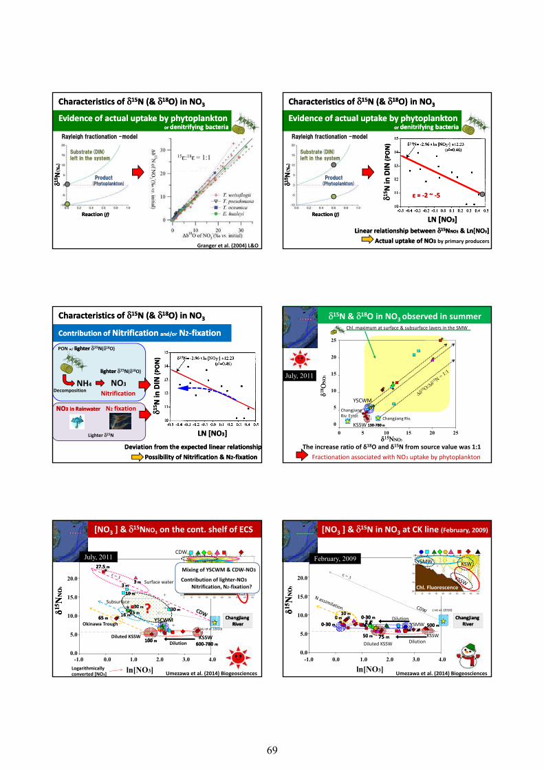
Substrate(DIN)left in the system
((‰‰
))
Rayleigh fractionation -model
Evidence of actual uptake by phytoplanktonEvidence of actual uptake by phytoplankton
Characteristics of Characteristics of δδ1515N (& N (& δδ1818O) in NOO) in NO33
or or denitrifying bacteriadenitrifying bacteria
15ε:18ε = 1:1
ReactionReaction ((f)f)
Product (Phytoplankton)δδ1515
NN((
Granger et al. (2004) L&O
Substrate(DIN)left in the system
((‰‰
))
DIN
DI
N (P
ON
)(P
ON
)
Rayleigh fractionation -model
Evidence of actual uptake by phytoplanktonEvidence of actual uptake by phytoplankton
Characteristics of Characteristics of δδ1515N (& N (& δδ1818O) in NOO) in NO33
or or denitrifying bacteriadenitrifying bacteria
ReactionReaction ((f)f)
Product (Phytoplankton)δδ1515
NN((
LN [NOLN [NO33]]
δδ1515N
in D
N in
D
ε = ε = --2 ~2 ~ --5 5
Linear relationship between Linear relationship between δδ1515NNNONO33 & & LnLn[NO[NO33]]Actual uptake of NOActual uptake of NO33 by primary producers
DIN
DI
N (P
ON
)(P
ON
)
Contribution of Contribution of NitrificationNitrification and/orand/or NN22--fixation fixation
Characteristics of Characteristics of δδ1515N (& N (& δδ1818O) in NOO) in NO33
PON w/ lighterlighter δ15N(δ18O)
NH4 NO3
lighter lighter δ15N(δ18O)
LN [NOLN [NO33]]
δδ1515N
in D
N in
D
Deviation from the expected linear relationshipDeviation from the expected linear relationshipPossibility of Nitrification & NPossibility of Nitrification & N22--fixationfixation
Decomposition NitrificationNH4 NO3
Lighter δ15N
N2 fixationNONO33 in Rainwaterin Rainwater
25
20
15
*
*
*July, 2011
OON
ON
O33
δ15N & δ18O in NO3 observed in summerChl. maximum at surface & subsurface layers in the SMW
0 5 10 15 20 25
10
5
0
YSCWM
KSSW 130130--780 780 mmChangjiang Riv.
ChangjiangRiv. Estur.
* *
δδ1515NNNONO33
δδ1818OO
The increase ratio of δ18O and δ15N from source value was 1:1Fractionation associated with NO3 uptake by phytoplankton
3 3 mm
10 10 mm
27.5 27.5 mm
3 3 mm Surface water
*
NNN
ON
O33
25.0
20.0
15.0
July, 2011
Chl. Fluorescence KSSW
YSCWM
CDW
Mixing of YSCWM & CDW-NO3
Contribution of lighter-NO3Nitrification, N2-fixation?
[NO3 ] & δ15NNO3 on the cont. shelf of ECS
-1.0 0.0 1.0 2.0 3.0 4.0
ln[NO3]
16 16 mm30 30 mm30 30 mm
25 25 mm65 65 mm
KSSWDilution
YSCWM
Diluted KSSW
Subsurface
600600--780 780 mm100 100 mm
Okinawa Trough
***
Li et al. (2010)
δδ1515NN 15.0
10.0
5.0
0.0
ChangjiangChangjiangRiverRiver
??
Umezawa et al. (2014) BiogeosciencesLogarithmically converted [NO3]
NNN
ON
O33
25.0
20.0
15.0
KSSWChl. Fluorescence
YSMW
[NO3 ] & δ15N in NO3 at CK line (February, 2009)
February, 2009KSW
-1.0 0.0 1.0 2.0 3.0 4.0
ln[NO3]
δδ1515NN 5.0
10.0
5.0
0.0
50 50 mm
00--30 30 mm0 0 mm
10 10 mm
75 75 mm
00--30 30 mm
Dilution
DilutionYSMW
KSSW
500 500 mm
Diluted KSSW
** **
Li et al. (2010)
ChangjiangChangjiangRiverRiver
Umezawa et al. (2014) Biogeosciences
69
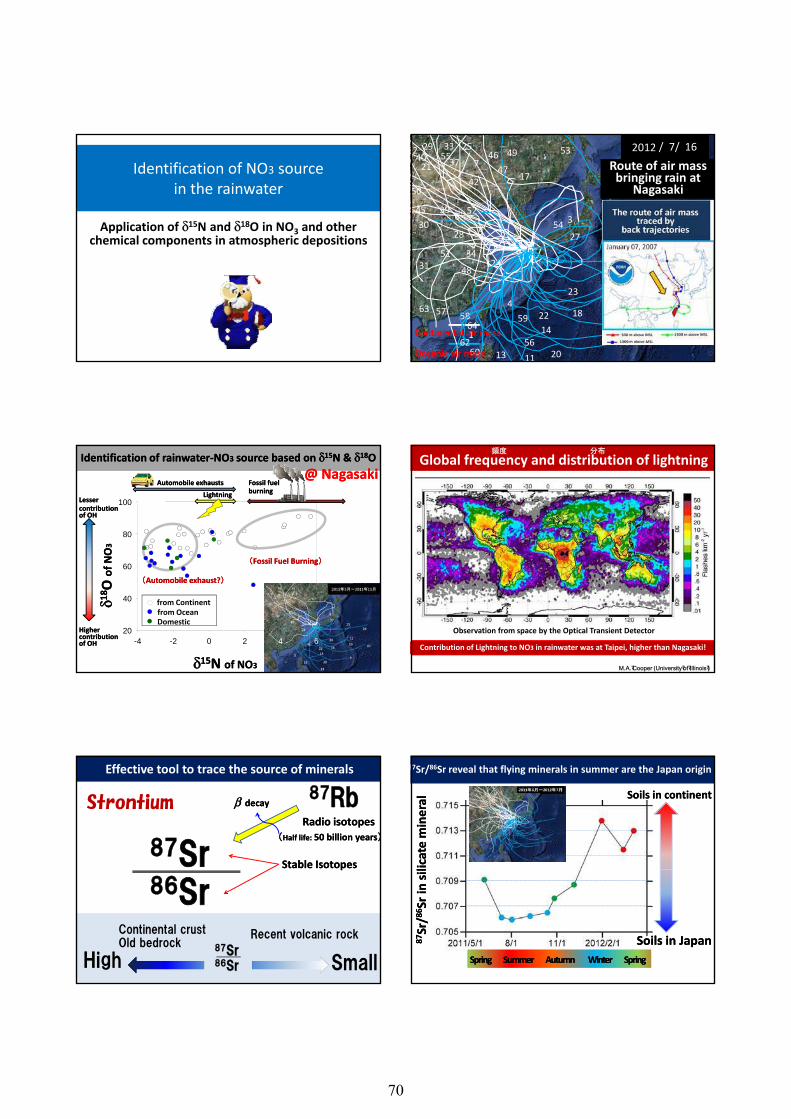
Identification of NO3 source in the rainwater
Application of δ15N and δ18O in NO3 and other chemical components in atmospheric depositions
2011 / 5/ 232011 / 5/ 232011 / 5/ 30
3
2011 / 6/ 5
5
2011 / 6/ 7
6
2011 / 6/ 87
2011 / 6/ 142011 / 6/ 152011 / 6/ 212011 / 6/ 232011 / 6/ 272011 / 6/ 302011 / 7/ 42011 / 7/ 6
15
2011 / 7/ 122011 / 7/ 13
17
2011 / 7/ 202011 / 8/ 12011 / 8/ 82011 / 8/ 16
21
2011 / 8/ 202011 / 8/ 232011 / 8/ 242011 / 9/ 2925 2011 / 10/ 32011 / 10/ 5
27
2011 / 10/ 14
28
2011 / 10/ 1529 2011 / 10/ 20
30
2011 / 11/ 22011 / 11/ 102011 / 11/ 1832 33 2011 / 11/ 232011 / 12/ 8
5
2011 / 1/ 162011 / 1/ 1837
2011 / 1/ 252011 / 2/ 1
39
2011 / 2/ 740
2011 / 2/ 13
1
2011 / 2/ 15
42
2011 / 2/ 222011 / 3/ 12011 / 3/ 5
45
2011 / 3/ 1846
2011 / 3/ 23
47
2011 / 3/ 252011 / 4/ 349 2011 / 4/ 11
50
2011 / 4/ 132011 / 4/ 25
52
2011 / 5/ 1453 2011 / 5/ 22
54
2011 / 5/ 2555
2011 / 6/ 72011 / 6/ 182011 / 6/ 212011 / 6/ 242011 / 6/ 272011 / 7/ 32011 / 7/ 52011 / 7/ 112011 / 7/ 122011 / 7/ 16
Route of air mass bringing rain at
Nagasaki
2012
1
4
9
10
11
12
13
14
1516
1819
20
22
23
243134
4
48
51
56
57 58 59
60
6162
63
64Continental air mass
Oceanic air mass
NO
NO
33
Automobile Automobile exhaustsexhausts Fossil fuel Fossil fuel burningburning
LesserLessercontribution contribution of OHof OH
@ Nagasaki@ Nagasaki
80
100
Identification of rainwaterIdentification of rainwater--NONO33 source based on source based on δδ1515N & N & δδ1818OO
LightningLightning
((F il F l B iF il F l B i ))
δδ1515N N of NOof NO33
δδ1818O
O
of Nof N
from Continentfrom Ocean
((Automobile exhaust?Automobile exhaust?))
Higher Higher contribution contribution of OHof OH -4 -2 0 2
20
40
60
4 6
Domestic
((Fossil Fuel BurningFossil Fuel Burning))
Global frequency and distribution of lightning 頻度 分布
Observation from space by the Optical Transient Detector
M.A. Cooper (University of Illinois )
Contribution of Lightning to NO3 in rainwater was at Taipei, higher than Nagasaki!
87Sr
Strontium
Stable IsotopesStable Isotopes
87RbRadio isotopesRadio isotopes
((Half life: Half life: 50 billion years50 billion years))
ββ decaydecay
Effective tool to trace the source of minerals
86Srpp
87Sr86SrHigh
Continental crustOld bedrock
Recent volcanic rock
Small
87Sr/86Sr reveal that flying minerals in summer are the Japan origin
Soils in continentSoils in continent
licat
e m
iner
allic
ate
min
eral
SpringSpring SummerSummer AutumnAutumn WinterWinter SpringSpring
8787Sr
/Sr
/8686Sr
in si
lSr
in si
l
Soils in JapanSoils in Japan
70
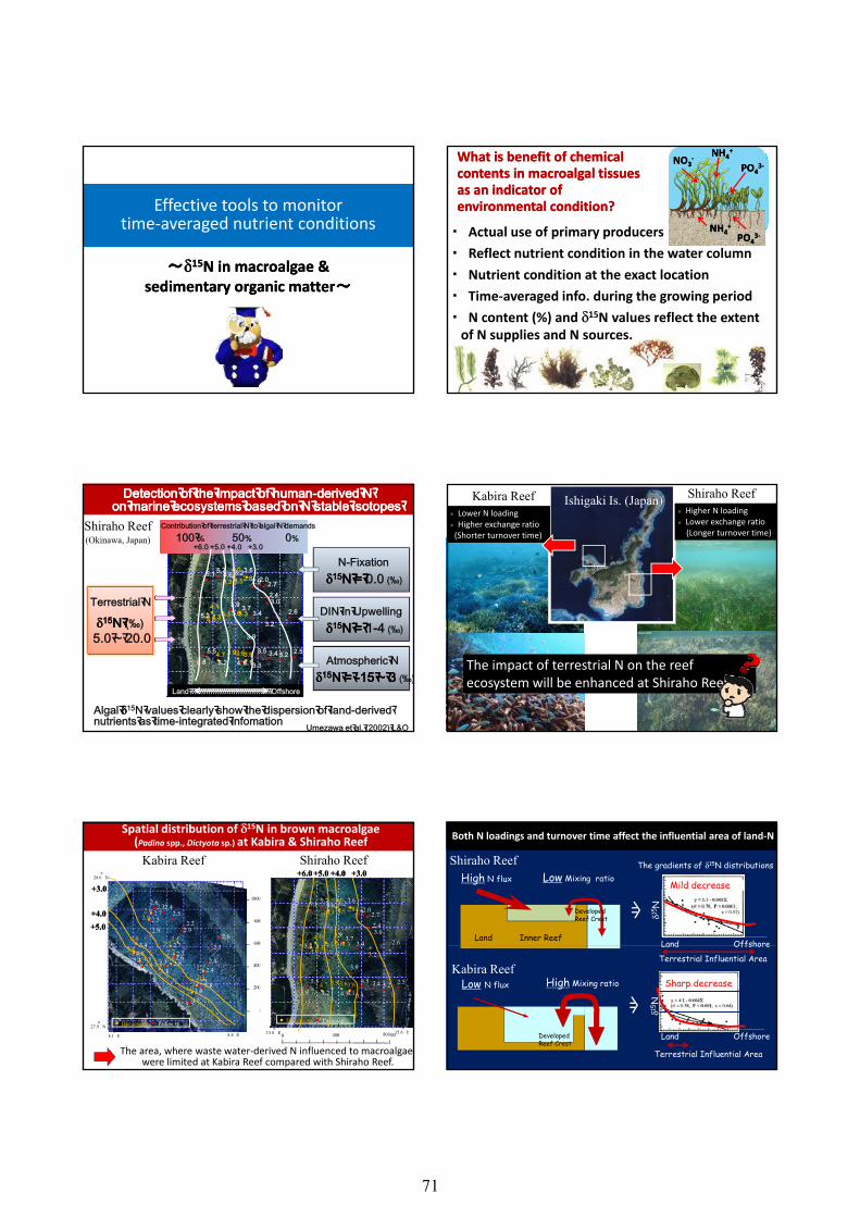
Effective tools to monitor time-averaged nutrient conditions
~~δδ1515N in macroalgae &N in macroalgae &δδ N in macroalgae & N in macroalgae & sedimentary organic mattersedimentary organic matter~~
What is benefitWhat is benefit of chemical of chemical contents in contents in macroalgalmacroalgal tissuestissuesas an indicator of as an indicator of environmental condition? environmental condition?
・ Actual use of primary producers・ Reflect nutrient condition in the water column
i di i h l i
NHNH44++
NONO33--
POPO4433--
δ15N N(%)
NHNH44++
NONO33--
POPO4433--
NHNH44++
POPO4433--
・ Nutrient condition at the exact location・ Time-averaged info. during the growing period・ N content (%) and δ15N values reflect the extent
of N supplies and N sources.
Detection of the impact of humanDetection of the impact of human--derived N derived N on marine ecosystems based on N stable isotopes on marine ecosystems based on N stable isotopes
Terrestrial N
100 % 50% 0%
5.1 5.74.6 3.23.62.92.0
2.72.43.0
3 73.9
4.3 3.52.84.0
4 1
+6.0 +4.0 +3.0+5.0
N-Fixationδδ1515N = N = 0.0 (‰)
DIN i U lli
Contribution of terrestrial N to algal N demandsShiraho Reef(Okinawa, Japan)
δδ1515N N (‰)5.0 ~ 20.0
Algal δδ15N values clearly show the dispersion of land-derived nutrients as time-integrated infomation
2.6
3.23.4
3.75.3
2.53.23.43.5
3.9
3.34.14.15.2
5.55.8
4.6
4.14.34.13.63.3
4.7 3.93.63.6
DIN in Upwellingδδ1515N N = = 1-4 (‰)
Atmospheric Nδδ1515N N = = --15 ~ 315 ~ 3 (‰)
Umezawa et al. (2002) L&O
Land Offshore
Shiraho ReefKabira Reef Ishigaki Is. (Japan)※ Lower N loading※ Higher exchange ratio(Shorter turnover time)
※ Higher N loading※ Lower exchange ratio
(Longer turnover time)
The impact of terrestrial N on the reefecosystem will be enhanced at Shiraho Reef
28.6°
N
3 4
2.9
2.52.7
2.62.3
2.52.4
2.22.9
2 72.6
2 3
+5.0+5.0
+4.0+4.0
+3.0+3.0
2.92.9
2.8 2.42.7
1000(m)
800
600
5.1 5.74.6 3.2 3.6
2.92.02.7
2.43.0
2.63.43.73.9
5 3
+6.0+6.0 +4.0+4.0 +3.0+3.0+5.0+5.0
4.3 3.5 2.84.0
4.14 3 4 1 3.63.3
Shiraho ReefKabira Reef
Spatial distribution of δ15N in brown macroalgae (Padina spp., Dictyota sp.) at Kabira & Shiraho Reef
27.9°
N
4.45.24.03.4 2.7
2.72.6
2.83.33.8
2.3
2.42.4
5.82.33.0
4.55.7
3.84.34.4
2.72.9
3.8 2.22.3
2.53.0
● Dictyota sp. ● Padina sp.
400
200
0
8.1°
E 8.8°
E 0 400 800(m)
3.25.3
2.53.23.43.5
3.9
3.34.14.15.2
5.5
5.8
4.64.3 4.1 3.3
4.7 3.9 3.63.6
● Dictyota sp. ● Padina sp.
15.0°
E 15.6°
E
The area, where waste water-derived N influenced to macroalgae,were limited at Kabira Reef compared with Shiraho Reef.
The gradients of δ15N distributions
Land Inner Reef
Both N loadings and turnover time affect the influential area of land-N
High N flux Low Mixing ratio
Developed Reef Crest
= δ15 N
Land Offshore
Shiraho Reef
Mild decrease
Low N flux High Mixing ratio
Terrestrial Influential Area
Developed Reef Crest
= δ15 N
Terrestrial Influential Area
Land Offshore
Land Offshore
Kabira Reef Sharp decrease
71
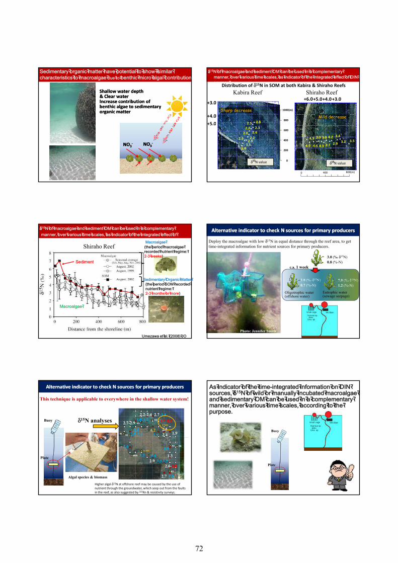
Sedimentary organic matter have potential to show similar characteristics to macroalgae due to benthic micro algal contribution
Shallow water depth Shallow water depth & Clear water& Clear waterIncrease contribution of Increase contribution of benthic algae to sedimentarybenthic algae to sedimentaryoorganic matter rganic matter
NONO33-- NONO33
--
+6.0 +4.0+3.0+5.0
δδ15N of macroalgae and sediment OM can be used in a complementary manner, over various time scales, as indicator of the integrated effect of DIN sources
1000(m)
800+5.0+4.0
+3.0
2.5 2.8
Shiraho ReefKabira Reef Distribution of δ15N in SOM at both Kabira & Shiraho Reefs
Mild decrease Sharp decrease
7.0
4.9
4.9
4.6
3.9
4.3
3.9
3.7
4.2
2.9
3.43.2 3.5
δ15N value
0 400 800(m)
600
400
200
0
+5.0
5.43.5
2.9 2.02.2
2.0 2.42.2 2.3
δ15N value
δδ15N of macroalgae and sediment OM can be used in a complementary manner, over various time scales, as indicator of the integrated effect of terrestrial DIN
Shiraho ReefMacroalgae
(the period macroalgae recorded nutrient regime: 2-3 weeks)
Sedimentary Organic Matter
Sediment
Umezawa et al. (2008) JO
y g(the period SOM recorded nutrient regime: 2-3 months or more)
Macroalgae
Alternative indicator to checAlternative indicator to check N sources for primary producersk N sources for primary producers
3.0 (‰ δ15N)0.8 (%-N)
3.0 (‰ δ15N) 7.0 (‰ δ15N)
c.a. 1 week
Deploy the macroalgae with low δ15N in equal distance through the reef area, to get time-integrated information for nutrient sources for primary producers.
Photo: Jennifer Smith
Eutrophic water (sewage seepage)
Oligotrophic water (offshore water)
3.0 (‰ δ N)0.7 (%-N)
7.0 (‰ δ N)1.2 (%-N)
Alternative indicator to check N sources for primary producersAlternative indicator to check N sources for primary producers
Buoy
2.2-2.4 2.7-3.4
2.7-2.93.0-3.2 4.3-5.2
3.4 4.23.92.5-3.4 2.4 1.9
2.5
δ15N analyses
This technique is applicable to everywhere in the shallow water system!
Plate
2.6 4.0
3.4 1.32.9 3.5 3.5
2.6-5.8
2.7 3.5
3.3
Higher algal δ15N at offshore reef may be caused by the use of nutrient through the groundwater, which seep out from the faults in the reef, as also suggested by 222Rn & resistivity surveys.
Algal species & biomass
As indicator of the time-integrated information on DIN sources, δδ15N of wild or manually incubated macroalgae and sedimentary OM can be used in a complementary manner, over various time scales, according to the purpose.
72
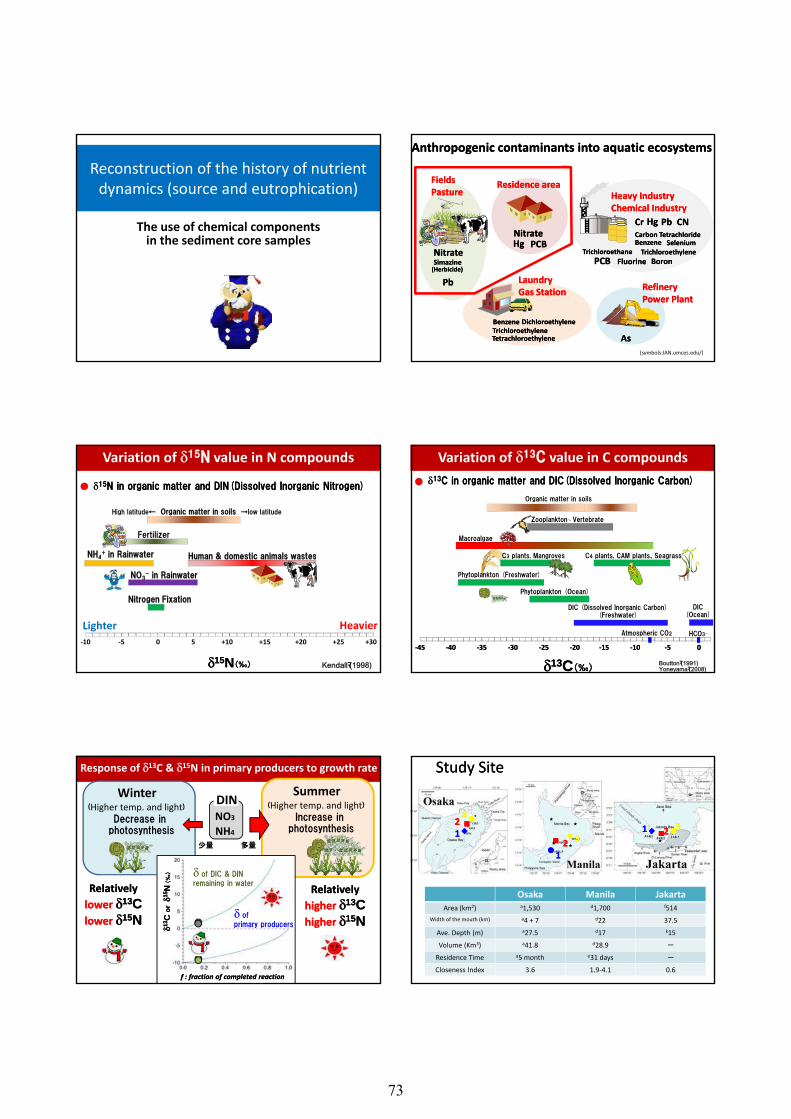
Reconstruction of the history of nutrient dynamics (source and eutrophication)
The use of chemical components in the sediment core samples
CNCNPbPbCrCr HgHgCarbon TetrachlorideCarbon TetrachlorideBenzeneBenzene SeleniumSelenium
Heavy IndustryHeavy IndustryChemical IndustryChemical Industry
PCBPCBHgHg
Residence areaResidence area
Anthropogenic contaminants into aquatic ecosystems Anthropogenic contaminants into aquatic ecosystems
Fields Fields PasturePasture
NitrateNitrate
(symbols:IAN.umces.edu/)
FluorineFluorine BoronBoronTrichloroethaneTrichloroethane TrichloroethyleneTrichloroethylene
PCBPCB
gg
AsAs
RefineryRefineryPower PlantPower Plant
(Herbicide)(Herbicide)SimazineSimazine
PbPb LaundryLaundryGas StationGas Station
BenzeneBenzeneTrichloroethyleneTrichloroethyleneTetrachloroethyleneTetrachloroethylene
DichloroethyleneDichloroethylene
NitrateNitrate
Variation of δ15N value in N compounds
δδ1515N in organic matter and DIN(Dissolved Inorganic Nitrogen)N in organic matter and DIN(Dissolved Inorganic Nitrogen)
High latitude← Organic matter in soils →low latitude
Human & domestic animals wastes
Fertilizer
NH4+ in Rainwater
-10 -5 0 5 +10 +15 +20 +25 +30
NO3- in Rainwater
Kendall (1998)
Human & domestic animals wastes
Nitrogen Fixation
Lighter Heavier
δδ1515NN((‰‰))
C4 plants, CAM plants、Seagrass
Macroalgae
C3 plants, Mangroves
Zooplankton~ Vertebrate
Organic matter in soils
Variation of δ13C value in C compoundsδδ1313C in organic matter and DIC(Dissolved Inorganic Carbon)C in organic matter and DIC(Dissolved Inorganic Carbon)
--45 45 --40 40 --35 35 --30 30 --25 25 --20 20 --15 15 --10 10 --5 5 0 0
HCO3-Atmospheric CO2
DIC (Dissolved Inorganic Carbon)(Freshwater)
p p gp g
Phytoplankton (Ocean)
Phytoplankton (Freshwater)
Boutton (1991)Yoneyama (2008)
DIC(Ocean)
δδ1313CC((‰‰))
Response of δ13C & δ15N in primary producers to growth rate
NO3
NH4
Summer(Higher temp. and light)
Increase in photosynthesis
多量少量
DINWinter(Higher temp. and light)
Decrease in photosynthesis
δRelativelyRelatively
higherhigher δδ1313CChigherhigher δδ1515NN
RelativelyRelativelylowerlower δδ1313CClowerlower δδ1515NN
f : fraction of completed reactionf : fraction of completed reaction
δ of DIC & DINremaining in water
δ of primary producersδδ1313
C
C o
rorδδ1515
NN((‰‰
))
Study SiteStudy Site
★
★
★
◆◆■■
●●
◆◆■■
●●
◆◆ ■■ ●●
★
★
1122
33
332211
11 22 33
Osaka Manila JakartaArea (km2) a1,530 d1,700 f514
Width of the mouth (km) a4 + 7 d22 37.5
Ave. Depth (m) a27.5 d17 k15
Volume (Km3) a41.8 d28.9 -
Residence Time a5 month e31 days -
Closeness Index 3.6 1.9-4.1 0.6
73
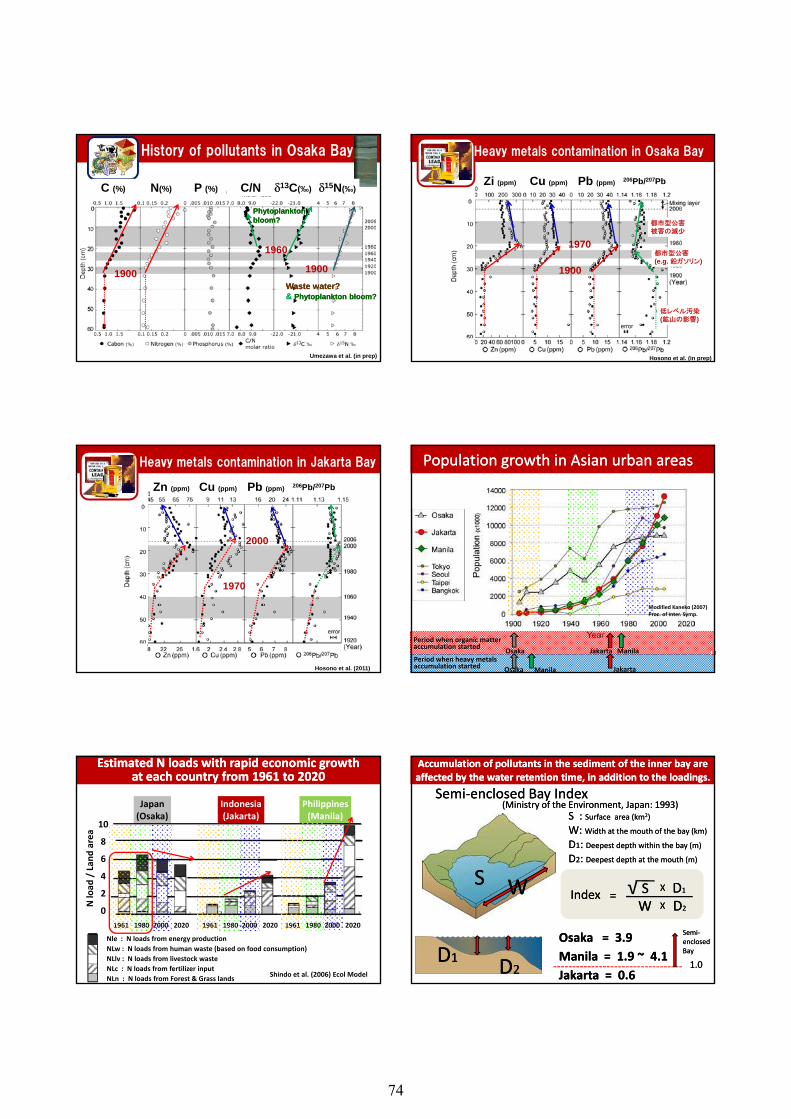
Phytoplankton Phytoplankton bloom?bloom?
1960
C (%) N(%) P (%) C/N δ13C(‰) δ15N(‰)
History of pollutants in Osaka Bay
Umezawa et al. (in prep)
1900Waste water?Waste water?& & Phytoplankton bloom?Phytoplankton bloom?
1960
1900
Heavy Metals in Osaka Bay
1970
都市型公害被害の減少
Zi (ppm) Cu (ppm) Pb (ppm) 206Pb/207Pb
Heavy metals contamination in Osaka Bay
Hosono et al. (in prep)
低レベル汚染(鉱山の影響)
1900
都市型公害(e.g. 鉛ガソリン)
2000
Heavy metals contamination in Jakarta Bay
Zn (ppm) Cu (ppm) Pb (ppm) 206Pb/207Pb
Hosono et al. (2011)
1970
Population growth in Asian urban areasPopulation growth in Asian urban areas
Modified Kaneko (2007) Proc. of Inter. Symp.
Osaka Jakarta ManilaPeriod when organic matter accumulation started
Osaka JakartaManilaPeriod when heavy metals accumulation started
Indonesia(Jakarta)
Japan(Osaka)
Philippines(Manila)
Land
are
a
10
8
6
Estimated N loads with rapid economic growthEstimated N loads with rapid economic growthat each country from 1961 to 2020 at each country from 1961 to 2020
1961 1980 2000 2020 1961 1980 2000 2020 1961 1980 2000 2020
N lo
ad /
L 4
2
0
Shindo et al. (2006) Ecol Model
Nle : N loads from energy productionNLw : N loads from human waste (based on food consumption)NLlv : N loads from livestock wasteNLc : N loads from fertilizer inputNLn : N loads from Forest & Grass lands
SemiSemi--enclosed Bay Indexenclosed Bay Index(Ministry of the Environment, Japan: 1993)(Ministry of the Environment, Japan: 1993)
S : S : Surface area (kmSurface area (km22))
W: W: Width at the mouth of the bay (km)Width at the mouth of the bay (km)
DD11: : Deepest depth within the bay (m)Deepest depth within the bay (m)
DD22: : Deepest depth at the mouth (m)Deepest depth at the mouth (m)
Accumulation of pollutants in the sediment of the inner bay are Accumulation of pollutants in the sediment of the inner bay are affected by the water retention time, in addition to the loadings.affected by the water retention time, in addition to the loadings.
SS
DD11 DD22
WW SS√ XX DD11
DD22WW XXIndexIndex ==
Osaka = 3.9Osaka = 3.9Manila = 1.9 ~ 4.1Manila = 1.9 ~ 4.1Jakarta = 0.6Jakarta = 0.6
1.01.0
SemiSemi--enclosed enclosed BayBay
74
L5: Plankton Ecosystem Joji Ishizaka (Institute for Space-Earth Environmental Research, Nagoya University) Abstract
Freshwater discharge influences to plankton ecosystem of the coastal area. Freshwater is less saline and often low density, and the buoyancy effect makes the low salinity water is not easily mixed with seawater; however, entrainment and tidal pumping eventually mix the upper low salinity water with lower high salinity water. Freshwater discharge also supplies various organic and inorganic materials to coastal water. Loading of nutrients makes coastal water productive. Coastal area is also known as high population and activities by human. Large amount of nutrients loading and many constructions in shallow areas often caused eutrophication, red tides, hypoxia and other problems in the coastal area.
In this lecture, examples of changes of plankton ecosystem in coastal area by anthropogenic activities will be given. As the observation tool, satellite remote sensing technology is also summarized, and examples of the usage will be shown. One of the examples is the East China Sea which is the radically changing environment. One of the largest river in the world, Changjiang, influences to phytoplankton abundance and the taxonomic groups in the East China Sea. Increasing anthropogenic nutrient loading as well as large sediment discharge and accumulated sediment seems to be very important for the ecosystem.
75
jimu
タイプライターテキスト

76
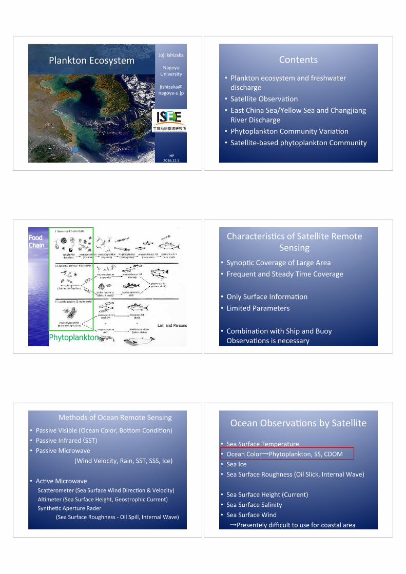
IHP$2016.12.5�
Plankton$Ecosystem�Joji$Ishizaka$$
$Nagoya$$
University$$
jishizaka@$nagoyaBu.jp�
Contents�
• Plankton$ecosystem$and$freshwater$discharge$
• Satellite$ObservaLon$• East$China$Sea/Yellow$Sea$and$Changjiang$River$Discharge$
• Phytoplankton$Community$VariaLon$
• SatelliteBbased$phytoplankton$Community$
Food Chain
Lalli and Parsons
Phytoplankton�
CharacterisLcs$of$Satellite$Remote$Sensing;$
• SynopLc$Coverage$of$Large$Area$• Frequent$and$Steady$Time$Coverage$
• Only$Surface$InformaLon$
• Limited$Parameters$
• CombinaLon$with$Ship$and$Buoy$ObservaLons$is$necessary$
Methods$of$Ocean$Remote$Sensing�
• Passive$Visible$(Ocean$Color,$Bo[om$CondiLon);$
• Passive$Infrared$�SST);�• Passive$Microwave$$
$$$$$$$$$$$$$$$$$$$$$$$$$$$$(Wind$Velocity,$Rain,$SST,$SSS,$Ice);$
;;;;;;;;;;;;;;;;;;;;;;;;;;;;�
• AcLve$Microwave;�Sca[erometer$(Sea$Surface$Wind$DirecLon$&$Velocity)�
AlLmeter$(Sea$Surface$Height,$Geostrophic$Current);�
SyntheLc$Aperture$Rader$$
$$$$$$$$$$$$$(Sea$Surface$Roughness$B$Oil$Spill,$Internal$Wave)$
e�
Ocean$ObservaLons$by$Satellite$$�
• Sea$Surface$Temperature$
• Ocean$Color9Phytoplankton,$SS,$CDOM$
• Sea$Ice;$• Sea$Surface$Roughness$(Oil$Slick,$Internal$Wave)$
• Sea$Surface$Height$(Current);$• Sea$Surface$Salinity;$• Sea$Surface$Wind$
;��9Presentely$difficult$to$use$for$coastal$area$
�
jimu
タイプライターテキスト
77
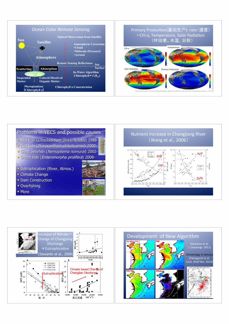
Sea Surface
Sun
Atmosphere
Satellite Optical Observation from Satellite
Chlorophyll a Concentration
Atmospheric Correction �Cloud �Molecule (Pressure���Aerosol
In-Water Algorithm Chlorophyll ��f (Rrs)
Remote Sensing Reflectance
Suspended Matter
Colored Dissolved Organic Matter
Scattering Absorption
Phytoplankton �Chlorophyll a�
Ocean&Color&Remote&Sensing� Primary$ProducLon(����)B$rateB��C$:ChlBa,$Temperature,$Solar$RadiaLon$
;B���< �<�C$
Solar$RadiaLon� Primary$ProducLon�
ChlBa� Temperature�
Problems in YECS and possible causes�
• Red tide (Choclodinium polykrikoides) 1988- • Red tide (Prorocentram shikokuense) 2000- • Giant Jellyfish (Nemopilema nomurai) 2002- • Green tide (Enteromorpha prolifera) 2008-
• Eutrophication (River, Atmos.) • Climate Change • Dam Construction • Overfishing • More
Chugoku News
Iwataki
Nutrient$Increase$in$Changjiang$River8BWang$et$al.,$2006C�
DIN�
DIP�
Si�
Si/N�
N/P�
Increase$of$Nitrate$:$Change$of$Changjiang$
Discharge$DEutrophicaLon$
(Siswanto et al., 2008)
Eutrophication Climate based Change of Changjian Discharge
;�;�;� ;����;�
Development$$of$New$Algorithm�
��1�
���1�
#*2�
Standard CHL�
)& � "$� !/--,4,2+,�
('%�
(Siswanto$et$al.$$J.$Oceanogr.$2011)�
$Climatology$in$January$$$
(Yamaguchi$et$al.$$Cont.$Shelf$Res.$2013)$
jimu
タイプライターテキスト
78
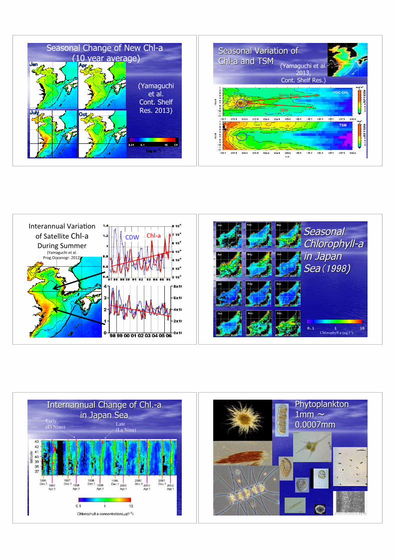
10 year average of OC and OC+TS2 Chl-a
Seasonal Change of New Chl-a (10 year average)
(Yamaguchi et al.
Cont. Shelf Res. 2013)
#*2� �34�
&+5�#607�
��1.�1�������
Seasonal Variation of Chl-a and TSM
YOC CHL
TSM
Spring Bloom
CDW
(Yamaguchi et al. 2013,
Cont. Shelf Res.)
Interannual$VariaLon$$of$Satellite$ChlBa$During$Summer$
(Yamaguchi$et$al.$Prog.Oceanogr.$2012)�
CDW� ChlBa�
Nov.50
45
40
35
130 135 140
Oct.50
45
40
35
130 135 140
Dec.50
45
40
35
130 135 140
50
45
40
35
130 135 140
Sep.50
45
40
35
130 135 140
Aug.50
45
40
35
Jul.
130 135 140
50
45
40
35
130 135 140
Jun.50
45
40
35
130 135 140
May.50
45
40
35
130 135 140
Apr.
50
45
40
35
130 135 140
Mar.50
45
40
35
130 135 140
Feb.50
45
40
35
130 135 140
Jan.
Seasonal Chlorophyll-a in Japan Sea�����)
0.1 1 10 Chlorophyll a (µg l-1)
�
Internannual Change of Chl.-a in Japan Sea
�=��>@A? =��>@A?
Late (La Nina)
Early (El Nino)
Phytoplankton 1mm E 0.0007mm�
jimu
タイプライターテキスト
79
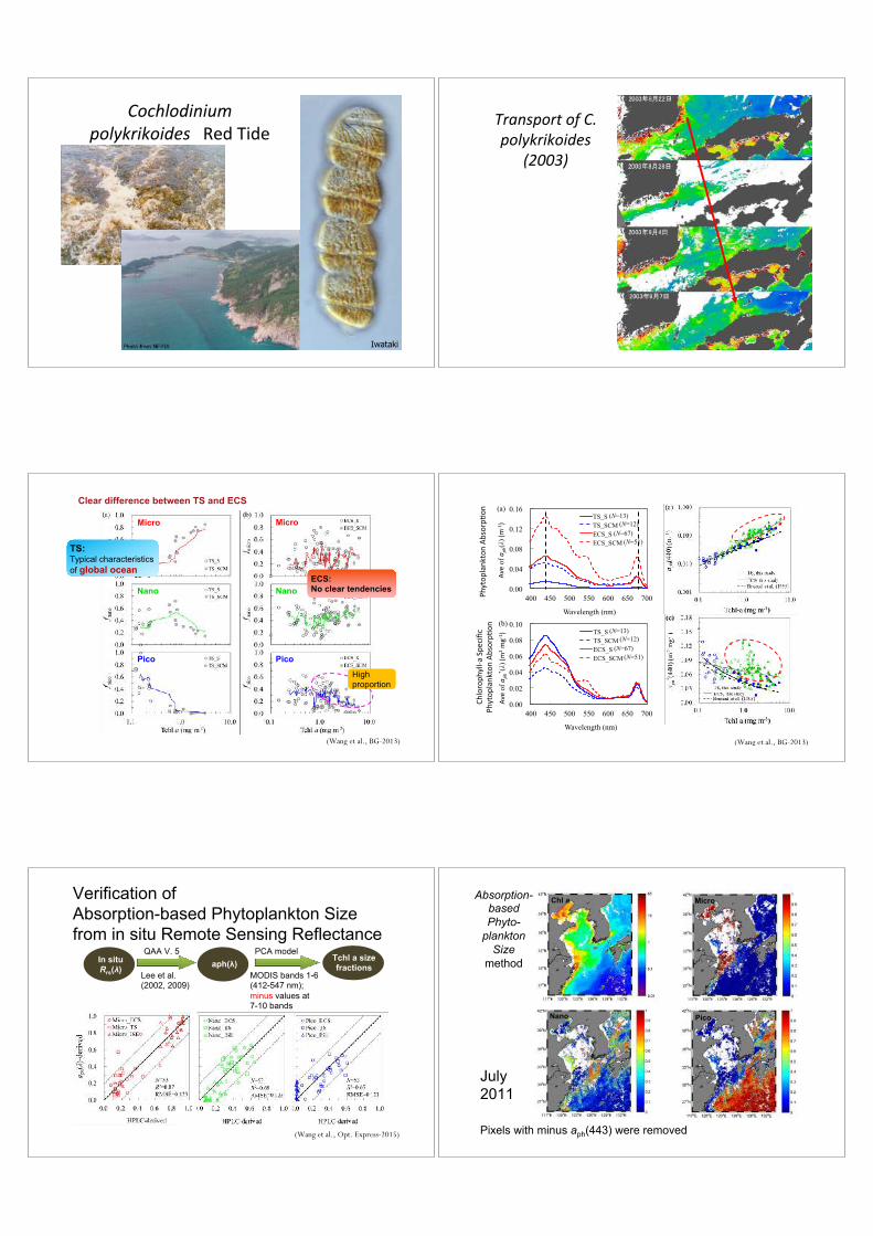
Cochlodinium&polykrikoides;Red$Tide�
Iwataki�
Transport&of&C.&polykrikoides&
(2003)�
Micro Micro
Nano Nano
Pico Pico
TS: Typical characteristics of global ocean
ECS: No clear tendencies
Clear difference between TS and ECS
High proportion�
(Wang et al., BG-2013)
Chloroph
yllBa
$Spe
cific$
Phytop
lankton$AbsorpL
on�
0.00
0.04
0.08
0.12
0.16
400 450 500 550 600 650 700
Ave$o
f aph
(λ)$(m
B1)$
Wavelength (nm)
TS_S (N=13) TS_SCM (N=12) ECS_S (N=67) ECS_SCM (N=51)
(a)�(N=13)
(N=12) (N=67)
(N=51)
0.00
0.02
0.04
0.06
0.08
0.10
400 450 500 550 600 650 700
Ave&o
f aph
* (λ)$(m
2 $mgB1 )$
Wavelength (nm)
TS_S (N=13) TS_SCM (N=12) ECS_S (N=67) ECS_SCM (N=51)
(b)�(N=13)
(N=12) (N=67)
(N=51)
TS_S TS_SCM ECS_S ECS_SCM
Magnitude
Distinct peaks in the blue and red band
Distinct difference both in magnitude and spectrum shape
TS_S
TS_SCM
ECS_S
ECS_SCM Magnitude at blue bands
(Wang et al., BG-2013)
Phytop
lankton$AbsorpL
on�
Verification of Absorption-based Phytoplankton Size from in situ Remote Sensing Reflectance
In situ Rrs(λ) aph(λ)
Tchl a size fractions
QAA V. 5
Lee et al. (2002, 2009)
PCA model
MODIS bands 1-6 (412-547 nm); minus values at 7-10 bands
(Wang et al., Opt. Express-2015)
July 2011�
Chl a� Micro�
Nano� Pico�
Absorption-based Phyto-
plankton Size
method�
Pixels with minus aph(443) were removed�
jimu
タイプライターテキスト
jimu
タイプライターテキスト
80
L6: Influence to Fisheries
Satoshi Ishikawa (Research Department, Research Institute for Humanity and Nature)
Abstract
In East Asia including Southeast Asian countries, approximate 72 % of 2 billion people living in
rural and urban areas in coastal zone. Livelihoods in rural area are based on various ecosystem
services provided from coastal nature that has high productivity and biodiversity, e.g.,
Mangrove trees are utilized for building materials and fuels, fisheries resources has important
roles as protein and income sources. On the other hands, residents in urban area need some
foods from rural areas, and a market in a city is quite important for both rural and urban people.
Therefore, the connectivity and logistics between of them and economic activities are also
important elements when we think the sustainable developments in a coastal area.
Land use change associated with urbanization affects on freshwater discharges, and
subsequently on carrying capacity and biodiversity in coastal area, because most part of
minerals and materials for primary production being provided from lands with freshwater.
Besides, chemical contamination and increase of bacteria of freshwater in urban area can
endanger the food safety of fisheries products in coastal area. Keep sea food safety is quite
important for economic growth and improve quality of life in coastal zone.
Fisheries resource management is indispensable for sustainable development in coastal area.
However, high biodiversity and multiple fishing gears utilization make statistical data collection
difficult, even it is necessary for stock assessments. In addition, conservation of coastal habitats
of fisheries species are required for reproduction of the resources. Therefore, alternative way of
stock assessments and simultaneous conservation activities on coastal ecosystems are needed. In
this connection, community based fisheries resource utilization with scientific evaluation of
ecosystem health under collaboration among fisher folks, researchers and local governments are
proposed as a new approach for coastal development, names as “Area-capability (AC)”
approach.
In the AC approach, “care” of a target resources and its habitat, not management, is treated as
major activity. The care includes three aspects as follow, 1) cultivate interests on nature
supporting the target resources, 2) monitor the stock status based on daily utilization of the
resources, 3) cure actions on injured part of nature. Biological and ecological researches can
contribute to the cultivation of the interest of users, monitor of stock status and evaluation of
cure activities. The balance between community based utilization and care is most important in
coastal development. And the care of habitats should touch material flow, sanitation, logistics,
biodiversity, carrying capacity, cultural diversity, and education with human resource
81

development. This comprehensive development strengthen the resilience of areas against natural
disasters.
82
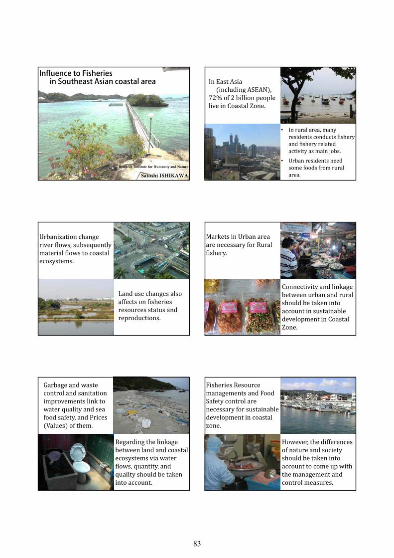
2016/10/5
1
Influence to Fisheries in Southeast Asian coastal area
Research Institute for Humanity and Nature
Satoshi ISHIKAWA
InEastAsiaincludingASEAN ,
72%of2billionpeopleliveinCoastalZone.
• Inruralarea,manyresidentsconductsfisheryandfisheryrelatedactivityasmainjobs.
• Urbanresidentsneedsomefoodsfromruralarea.
Urbanizationchangeriverflows,subsequentlymaterialflowstocoastalecosystems.
Landusechangesalsoaffectsonfisheriesresourcesstatusandreproductions.
MarketsinUrbanareaarenecessaryforRuralfishery.
ConnectivityandlinkagebetweenurbanandruralshouldbetakenintoaccountinsustainabledevelopmentinCoastalZone.
Garbageandwastecontrolandsanitationimprovementslinktowaterqualityandseafoodsafety,andPricesValues ofthem.
Regardingthelinkagebetweenlandandcoastalecosystemsviawaterflows,quantity,andqualityshouldbetakenintoaccount.
FisheriesResourcemanagementsandFoodSafetycontrolarenecessaryforsustainabledevelopmentincoastalzone.
However,thedifferencesofnatureandsocietyshouldbetakenintoaccounttocomeupwiththemanagementandcontrolmeasures.
83
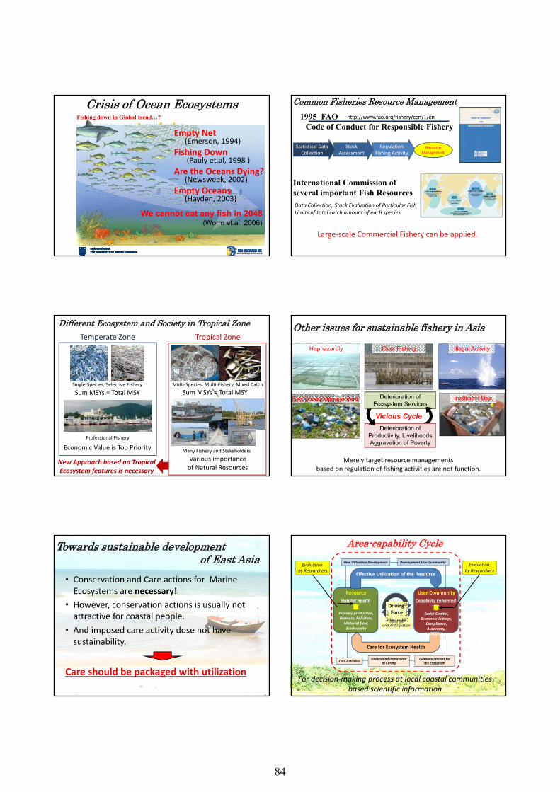
2016/10/5
2
Crisis of Ocean Ecosystems
Empty Net(Emerson, 1994)
Fishing Down(Pauly et.al, 1998 )
Are the Oceans Dying?(Newsweek, 2002)
Empty Oceans(Hayden, 2003)
Fishing down in Global trend…?
We cannot eat any fish in 2048 (Worm et.al, 2006)
1995 FAOCode of Conduct for Responsible Fishery
http://www.fao.org/fishery/ccrf/1/en
International Commission of several important Fish Resources
Large‐scale Commercial Fishery can be applied.
Common Fisheries Resource Management
Data Collection, Stock Evaluation of Particular FishLimits of total catch amount of each species
Regulation Fishing Activity
ResourceManagement
Stock Assessment
Statistical Data Collection
Different Ecosystem and Society in Tropical ZoneTemperate Zone Tropical Zone
Single‐Species, Selective Fishery Multi‐Species, Multi‐Fishery, Mixed CatchSum MSYs = Total MSY Sum MSYs = Total MSY
Economic Value is Top PriorityProfessional Fishery
Many Fishery and StakeholdersVarious importanceof Natural Resources
New Approach based on Tropical Ecosystem features is necessary
Other issues for sustainable fishery in Asia
Bad Waste Management Inefficient Use
Over Fishing Illegal ActivityHaphazardly
Vicious Cycle
Deterioration of Ecosystem Services
Deterioration of Productivity, LivelihoodsAggravation of Poverty
Merely target resource managements based on regulation of fishing activities are not function.
Towards sustainable development of East Asia
• Conservation and Care actions for Marine Ecosystems are necessary!
• However, conservation actions is usually not attractive for coastal people.
• And imposed care activity dose not have sustainability.
Care should be packaged with utilization
Resource User Community
Effective Utilization of the Resource
Care for Ecosystem Health
Driving Force
Cultivate Interest for the Ecosystem
Development User Community
Understand Importance of Caring
New Utilization Development
Care Activities
Pride, Hope and Anticipation
Primary production,Biomass, Pollution,
Material flow, Biodiversity
Social Capital,Economic linkage,
Compliance, Autonomy,
Management
Habitat Health Capability Enhanced
Evaluation by Researchers
Evaluation by Researchers
Area-capability Cycle
For decision‐making process at local coastal communities based scientific information
84
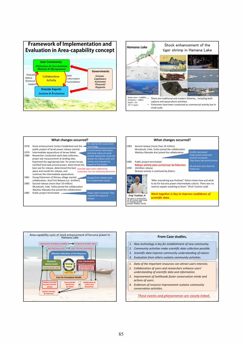
2016/10/5
3
User CommunityUtilizations & Care Activities
Monitors & Managements
Outside ExpertsAnalyses & Evaluations
GovernmentsLicense,
LegitimacyAutonomyFinancialSupports
DataInformationConsultation
Collaborative Activity
EvaluationAdviceTechnical
supports
Framework of Implementation and Evaluation in Area-capability concept
Stock enhancement of the tiger shrimp in Hamana Lake
Hamana Lake
Water area = 6,880haPeriphery = 128kmDepth = 5m 10th in Japan
• There are traditional and modern fisheries, including both capture and aquaculture activities.
• Fishermen have been conducted as commercial activity but in small scale.
What changes occurred?1978 Stock enhancement Center Established and the
public project of larval prawn release started.1979 Intermediate aquaculture of larvae failed. 1980 Researcher conducted catch data collection,
prawn size measurement at landing sites, Examined the appropriate bait for prawn larvae, clarified food web around prawn, determined the best size for release, determined the best place and month for release, and continue the intermediate aquaculture.
1981 Young fishermen of Shirasu village started collaboration. And First Release (ca. 3million).
1983 Second release (more than 10 million) Murakushi, Iride, Yutho joined the collaborationWashizu Maisaka Arai joined the collaboration
1985 Public project terminated
No appropriate aquaculture technology.Environmental information and stock status are quite limited. Researcher could not decide the release point and timing, and evaluate the impact of the project
No gain from release work but collaboration stated
Prawn catch increased. They realized the impact of release.
Scientific data were collected by researcher, but not utilized by fishermen
What changes occurred?1983 Second release (more than 10 million)
Murakushi, Iride, Yutho joined the collaborationWashizu Maisaka Arai joined the collaboration
1985 Public project terminated Release activity were carried over by fishermen
1990 14million releaseRelease activity is continued by fishers.
Conflict decreased. Trade system improved.Incomes increased.They knew lake environments
All activities were done by Fishermen
Prof. Fushimi, H Work together is Key to improve confidence of scientific data.
”After everything was finished,” fishers knew how and what to do for Kuruma prawn intermediate culture. There was no need to explain anything to them.” (Prof. Fushimi said)
He was a researcher at SE center and took in charge of the prawn release wrok.
Resource User Community
Effective Utilization of the Resource
Care for Ecosystem Health
Driving Force
Collaboration of Fishers and Researchers
Unify Fishermen Associations
Environmental Monitoring by Fishers
Stop Small prawn catch
Release JuvenilesBy governmental
project
Habitat Health Capability Enhanced
Increase prawn Stock Increase incomesDecrease conflicts
Release Juveniles By Fishermen
Hope, Pride
Improvement of market accessibility Involvement of other sectors
Area‐capability cycle of stock enhancement of Kuruma prawn in Hamana Lake From Case studies,
1. New technology is key for establishment of new community.2. Community activities make scientific data collection possible.3. Scientific data improve community understanding of nature.4. Evaluation from others sustains community activities.
1. Data of the important resources can attract users interests.2. Collaboration of users and researchers enhance users’
understanding of scientific data and information.3. Improvement of livelihoods foster conservation minds and
actions of users.4. Evidences of resource improvement sustains community
conservation activities.
These events and phenomenon are closely linked.
85
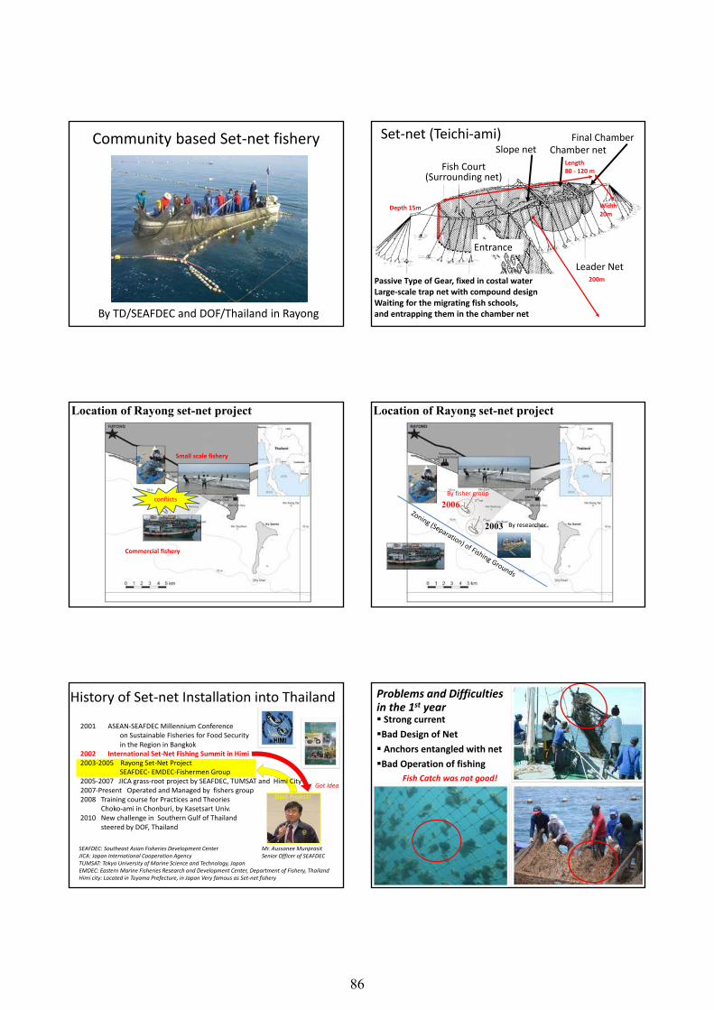
2016/10/5
4
Community based Set‐net fishery
By TD/SEAFDEC and DOF/Thailand in Rayong
Fish Court(Surrounding net)
Entrance
Slope net Chamber netFinal ChamberSet‐net (Teichi‐ami)
Leader Net200m
Depth 15m
Length 80 ‐ 120 m
Width 20m
Passive Type of Gear, fixed in costal waterLarge‐scale trap net with compound designWaiting for the migrating fish schools, and entrapping them in the chamber net
Location of Rayong set-net project
conflicts
Small scale fishery
Commercial fishery
Location of Rayong set-net project
2003
2006By fisher group
By researcher
2001 ASEAN‐SEAFDEC Millennium Conferenceon Sustainable Fisheries for Food Security in the Region in Bangkok
2002 International Set‐Net Fishing Summit in Himi2003‐2005 Rayong Set‐Net Project
SEAFDEC‐ EMDEC‐Fishermen Group2005‐2007 JICA grass‐root project by SEAFDEC, TUMSAT and Himi City 2007‐Present Operated and Managed by fishers group2008 Training course for Practices and Theories
Choko‐ami in Chonburi, by Kasetsart Univ. 2010 New challenge in Southern Gulf of Thailand
steered by DOF, Thailand
History of Set‐net Installation into Thailand
SEAFDEC: Southeast Asian Fisheries Development CenterJICA: Japan International Cooperation AgencyTUMSAT: Tokyo University of Marine Science and Technology, JapanEMDEC: Eastern Marine Fisheries Research and Development Center, Department of Fishery, ThailandHimi city: Located in Toyama Prefecture, in Japan Very famous as Set‐net fishery
Mr. Aussanee MunprasitSenior Officer of SEAFDEC
Got Idea
Start Project!
Problems and Difficultiesin the 1st year� Strong current�Bad Design of Net� Anchors entangled with net�Bad Operation of fishing
Fish Catch was not good!
86
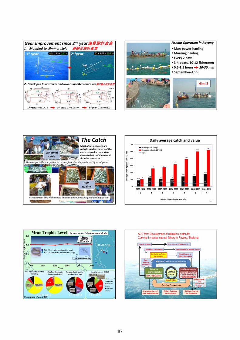
2016/10/5
5
1. Modified to slimmer style 身網の設計変更
Gear Improvement since 2nd year漁具設計改良
1st year 45 x 140 x 250 m 2ndyear 20 x 155 x 250 m
2. Developed to narrower and lower slope&entrance net昇り網の設計変更
1st year; 5.0x3.0x14 2nd year; 0.7x8.0x8.0 3rd year; 0.7x9.0x8.0
45
(Unit : m)
Fishing Operation in Rayong�Man‐power hauling�Morning hauling� Every 2 days� 3‐4 boats, 10‐12 fishermen� 0.5‐1.5 hours 20‐30 min� September‐April
Himi 2
Most of set‐net catch are pelagic species, variety of the catch showed an importantcharacteristics of the coastal fisheries resources.
Variety of catch
High quality
The Catch
Management Skill of them was improved through selling and pooling system
They caught different species by set‐net from that they collected by small gears.
28
175254 225 214
288 298352
210
516 551
634
782
10011041
52101 108 110 98 91 86
0
200
400
600
800
1000
1200
2003‐2004 2004‐2005 2005‐2006 2006‐2007 2007‐2008 2008‐2009 2009‐2010
1 2 3 4 5 6 7
Average catch (kg) and
value (THB
)
Year of Project Implementation
Daily average catch and value Average catch (Kg) Average value (x10 THB)trip
2.5
3.0
3.5
4.0
2003 2004 2005 2006 2007 2008Year
Mea
n Tr
ophi
cLe
vel
Mean Trophic Level Comparison
3.22 (Deep water bamboo stake trap) 3.15 (Shallow water bamboo stake trap)
3.04 (Sriracha set-net)
猪口網
Set‐net
(Aussanee et al., 2005)8-10 m depth 2-3 m depth 4-5 m depth
猪口網
1%
11%
29%
1%
58%
Sriracha set‐net
Chub mackerel
Carangidae
Valued fish
Other
Trash fishes
Shrimp
29
1% 2%
29%
14%
53%
Pangnga Shallow water bamboo stake trap
62%10%
24%
2% 2%
Chonburi Deep water bamboo stake trap
63%23%
4%2% 8%
Trad Deep water bamboo stake trap
THAILAND
, for gear design / fishing ground depth
Resource Local Community
Effective Utilization of Resource
Care for Ecosystems
Driving Forces
Cultivate interest for Ecosystem
Establishment of Fishers Community
Fishery Statistical data collection
Set‐Net Installation by SEAFDEC
Environmental and Food Web estimation
Improved Status Enhanced Capability
New Target Species New Markets, Decrease conflicts
Hopes, Prides
Community Fish Market Improvement of Trading system
Management Skill
Operational Skill
Post Harvest
Technology
Tourism Activity Involvement of Other sectors
ACC from Development of utilization methods: Community-based set-net fishery in Rayong, Thailand.
87
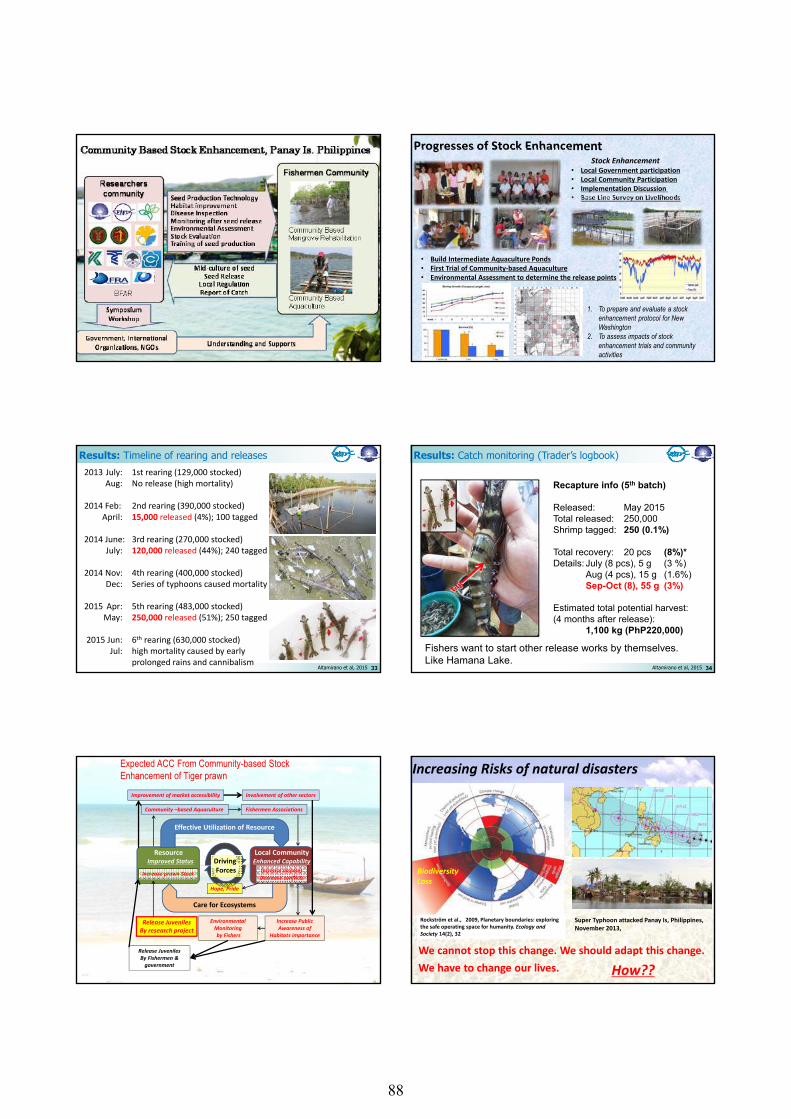
2016/10/5
6
Progresses of Stock EnhancementStock Enhancement
• Local Government participation• Local Community Participation• Implementation Discussion • Base Line Survey on Livelihoods
1. To prepare and evaluate a stock enhancement protocol for New Washington
2. To assess impacts of stock enhancement trials and community activities
• Build Intermediate Aquaculture Ponds• First Trial of Community‐based Aquaculture• Environmental Assessment to determine the release points
33Altamirano et al, 2015
2013 July: 1st rearing (129,000 stocked)Aug: No release (high mortality)
2014 Feb: 2nd rearing (390,000 stocked)April: 15,000 released (4%); 100 tagged
2014 June: 3rd rearing (270,000 stocked)July: 120,000 released (44%); 240 tagged
2014 Nov: 4th rearing (400,000 stocked)Dec: Series of typhoons caused mortality
2015 Apr: 5th rearing (483,000 stocked)May: 250,000 released (51%); 250 tagged
2015 Jun: 6th rearing (630,000 stocked)Jul: high mortality caused by early
prolonged rains and cannibalism
Results: Timeline of rearing and releases
34Altamirano et al, 2015
Recapture info (5th batch)
Released: May 2015Total released: 250,000Shrimp tagged: 250 (0.1%)
Total recovery: 20 pcs (8%)*Details: July (8 pcs), 5 g (3 %)
Aug (4 pcs), 15 g (1.6%)Sep-Oct (8), 55 g (3%)
Estimated total potential harvest:(4 months after release):
1,100 kg (PhP220,000)
Results: Catch monitoring (Trader’s logbook)
Fishers want to start other release works by themselves. Like Hamana Lake.
Resource Local Community
Effective Utilization of Resource
Care for Ecosystems
Driving Forces
Increase Public Awareness of
Habitats importance
Fishermen Associations
Environmental Monitoring by Fishers
Community –based Aquaculture
Release JuvenilesBy research project
Improved Status Enhanced Capability
Increase prawn Stock Increase incomesDecrease conflicts
Release Juveniles By Fishermen & government
Hope, Pride
Improvement of market accessibility Involvement of other sectors
Expected ACC From Community-based Stock Enhancement of Tiger prawn Increasing Risks of natural disasters
Rockström et al., 2009, Planetary boundaries: exploring the safe operating space for humanity. Ecology and Society 14(2), 32
Biodiversity Loss
Super Typhoon attacked Panay Is, Philippines, November 2013,
We cannot stop this change. We should adapt this change.We have to change our lives. How??
88
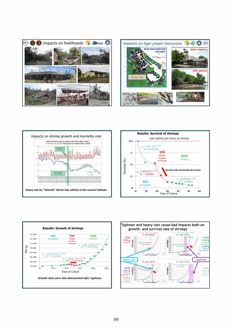
2016/10/5
7
Impacts on livelihoodsBefore typhoon
After typhoon
Impacts on tiger prawn resources
Impacts on shrimp growth and mortality rate
Heavy rain by “Yolanda” derive low salinity in the coastal habitats.
Surv
ival
(%)
Days of Culture
STRSTRESS DURINGTYPHOON
ACCACCLIMATE
NORNORMAL
Results: Survival of shrimpsLow salinity put stress on shrimp
Survival rate drastically decreased
Results: Growth of shrimps
BW (g
)
Days of Culture
STRSTRESSDURING TYPHOON
ACCACCLIMATE
NOR(NORMAL)
Growth rates were also deteriorated after Typhoon.
[3rd]0.81 gat Day 30
(no typhoon)
[4th]0.61 gat Day 30
(no typhoon)
Typhoon and heavy rain cause bad impacts both on growth and survival rate of shrimps
[1st]0.34 gat Day 30
[2nd]0.40 gat Day 30
(no typhoon)
1st (Jul 2013) 2nd (Mar 2014)
3rd (Jun 2014) 4th (Nov 2014)
0.09 gat Day 30
(w/ typhoon)
0.30 gat Day 30
(w/ typhoon)
typhoonheavy rain
89
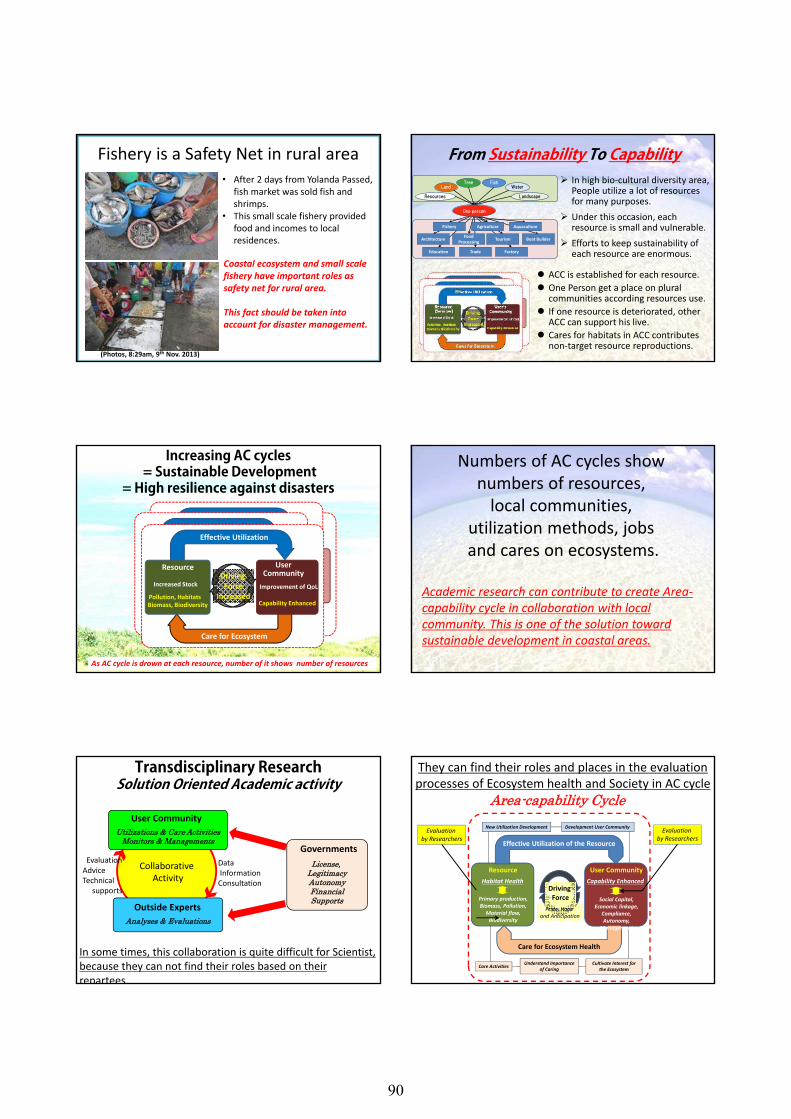
2016/10/5
8
Fishery is a Safety Net in rural area• After 2 days from Yolanda Passed,
fish market was sold fish and shrimps.
• This small scale fishery provided food and incomes to local residences.
Coastal ecosystem and small scale fishery have important roles as safety net for rural area.
This fact should be taken into account for disaster management.
(Photos, 8:29am, 9th Nov. 2013)
From Sustainability To CapabilityTree Fish
Land Water
LandscapeResources
Education Trade Factory
Boat BuilderFood Processing TourismArchitecture
AquacultureAgricultureFishery
One person
¾ In high bio‐cultural diversity area, People utilize a lot of resources for many purposes.
¾ Under this occasion, each resource is small and vulnerable.
¾ Efforts to keep sustainability of each resource are enormous.
z ACC is established for each resource.z One Person get a place on plural
communities according resources use.z If one resource is deteriorated, other
ACC can support his live.z Cares for habitats in ACC contributes
non‐target resource reproductions.
Effective Utilization
Care for Ecosystem
Improvement of QoLPollution, Habitats
UserCommunity
ResourceDriving Force
IncreasedBiomass, Biodiversity Capability Enhanced
Increased Stock
Increasing AC cycles= Sustainable Development
= High resilience against disasters
As AC cycle is drown at each resource, number of it shows number of resources
Numbers of AC cycles show numbers of resources, local communities,
utilization methods, jobsand cares on ecosystems.
Academic research can contribute to create Area‐capability cycle in collaboration with local community. This is one of the solution toward sustainable development in coastal areas.
User CommunityUtilizations & Care Activities
Monitors & Managements
Outside ExpertsAnalyses & Evaluations
GovernmentsLicense,
LegitimacyAutonomyFinancialSupports
DataInformationConsultation
Collaborative Activity
EvaluationAdviceTechnical
supports
Transdisciplinary Research Solution Oriented Academic activity
In some times, this collaboration is quite difficult for Scientist, because they can not find their roles based on their repartees.
Resource User Community
Effective Utilization of the Resource
Care for Ecosystem Health
Driving Force
Cultivate Interest for the Ecosystem
Development User Community
Understand Importance of Caring
New Utilization Development
Care Activities
Pride, Hope and Anticipation
Primary production,Biomass, Pollution,
Material flow, Biodiversity
Social Capital,Economic linkage,
Compliance, Autonomy,
Management
Habitat Health Capability Enhanced
Evaluation by Researchers
Evaluation by Researchers
Area-capability Cycle
They can find their roles and places in the evaluation processes of Ecosystem health and Society in AC cycle
90
2016/10/5
9
Catch from Rayongset-net
Biological Study
Yellow stripe scads Round herring Gar fish
Indian threadfish Trevally Spanish mackerel Black pomfret Barracuda Indian mackerel
Sailfish Rabbitfish Emperer Sea bream Threadfin bream Threadfin bream
Indo-pacific mackerel Yellowstrip scad Hairtail Wolf-herring Snapper Sardine
Leather jacket Leather jacket Blue swimming crab Bigfinreef squid Loligo squid Cuttlefish
49
2 Education Program, Submarine Robot Development, Environmental Survey
Anthoropologic Study and Robotics
2 Town Seminars, 2 Lectures of environment, 1 Exhibition at Museum
Collect data about behavior changes and information sharing through interviews
Stable Isotope Analysis show different units of Siganus javus in Bandon Bay δ15N (‰)
δ13C (‰)
Siganus javus
Central Area
West area
East Area
Chemical and Material flow Study
ShallwestartArea‐capabilitystudyaroundtheworld?Forourfuture!!
Thank you for your attentions!
91

92
L7: A Japanese experience of Tsunamis Takashi Tomita (Education and Research Center for Sustainable Co-Development, Graduate School of Environmental Studies, Nagoya University) Abstract Japan have learned many lessons from the 2011 Tohoku tsunami disaster: for example, multi-level
scenarios for disaster management and multi-layered measures to reduce possible disasters. Through
international cooperative research project, the Japanese experiences of tsunami disasters have been
introduced into Chile that is also in high risk areas of tsunamis. These Japanese experiences will be
introduced in the seminar.
93

94
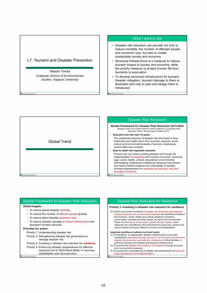
L7: Tsunami and Disaster Prevention
Takashi Tomita
Graduate School of Environmental Studies, Nagoya University
What I want to talk
• Disaster risk reduction can provide not only to reduce mortality, the number of affected people, and economic loss, but also to create sustainable society and economy.
• Structural infrastructure is a measure to reduce tsunami impact to society and economy, while the priority measure to protect human life from tsunamis is evacuation.
• To develop structural infrastructure for tsunami disaster mitigation, tsunami damage to them is illustrated and how to plan and design them is introduced.
Global Trend
Disaster Risk Reduction
• Outcome over the next 15 years:
The substantial reduction of disaster risk and losses in lives, livelihoods and health and in the economic, physical, social, cultural and environmental assets of persons, businesses, communities and countries.
• Goal to attain the expected outcome:
Prevent new and reduce existing disaster risk through the implementation of integrated and inclusive economic, structural, legal, social, health, cultural, educational, environmental, technological, political and institutional measures that prevent and reduce hazard exposure and vulnerability to disaster, increase preparedness for response and recovery, and thus strengthen resilience.
Sendai Framework for Disaster Risk Reduction 2015-2030 adopted at the Third United Nations World Conference on Disaster Risk
Reduction held in Sendai Japan in March 2015.
Sendai Framework for Disaster Risk ReductionGlobal targets:
– To reduce global disaster mortality,
– To reduce the number of affected people globally
– To reduce direct disaster economic loss
– To reduce disaster damage to critical infrastructure and disruption of basic services
Priorities for action:
Priority 1: Understanding disaster risk.
Priority 2: Strengthening disaster risk governance to manage disaster risk.
Priority 3: Investing in disaster risk reduction for resilience.
Priority 4: Enhancing disaster preparedness for effective response and to “Build Back Better” in recovery, rehabilitation and reconstruction.
Disaster Risk Reduction for Resilience
29. Public and private investment in disaster risk prevention and reduction through structural and non-structural measures are essential to enhance the economic, social, health and cultural resilience of persons, communities, countries and their assets, as well as the environment. These can be drivers of innovation, growth and job creation. Such measures are cost-effective and instrumental to save lives, prevent and reduce losses and ensure effective recovery and rehabilitation.
Priority 3: Investing in disaster risk reduction for resilience
Important activities at national and local levels:(c) To strengthen, as appropriate, disaster-resilient public and private
investments, particularly through structural, non-structural and functional disaster risk prevention and reduction measures in critical facilities, in particular schools and hospitals and physical infrastructures;
(e) To promote the disaster risk resilience of workplaces through structural and non-structural measures;
(f) To promote the mainstreaming of disaster risk assessments into land-use policy development and implementation;
95
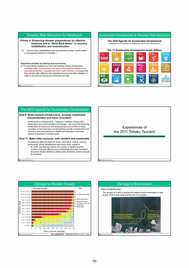
Disaster Risk Reduction for Resilience
Priority 4: Enhancing disaster preparedness for effective response and to “Build Back Better” in recovery, rehabilitation and reconstruction
Important activities at national and local levels:(c) To promote the resilience of new and existing critical infrastructure,
including water, transportation and telecommunications infrastructure, educational facilities, hospitals and other health facilities, to ensure that they remain safe, effective and operational during and after disasters in order to provide live-saving and essential services
32. --- the recovery, rehabilitation and reconstruction phase, which needs to be prepared ahead of a disaster, ---
Sustainable Development & Disaster Risk Reduction
The 2030 Agenda for Sustainable Development adopted at a UN Summit in September 2015 at an UN Summit
The 17 Sustainable Development Goals (SDGs)
The 2030 Agenda for Sustainable Development
Goal 9: Build resilient infrastructure, promote sustainable industrialization and foster innovation
Investments in infrastructure – transport, irrigation, energy and information and communication technology – are crucial to achieving sustainable development and empowering communities in many countries. It has long been recognized that growth in productivity and incomes, and improvements in health and education outcomes require investment in infrastructure.
Goal 11: Make cities inclusive, safe, resilient and sustainableConsidering cities are hubs for ideas, commerce, culture, science, productivity, social development and much more, a goal is:• By 2030, significantly reduce the number of deaths and the
number of people affected and substantially decrease the direct economic losses relative to global gross domestic product caused by disasters.
Experiences ofthe 2011 Tohoku Tsunami
Damage to Wooden Houses
国土交通省都市局 平成23年10月4日プレスリリースより
Wooden houses
Complete destruction
Almost destruction
Partial destructionInundation under the ground floorNo damage
Inun
datio
n de
pth
Ratio of houses damaged
Damage to Breakwaters
Port of HachinoheThe section of 1,400 m among the Hattaro North breakwater of total length 3500 m was destroyed by the 9 m tsunami.
Destroyed by wave force of the tsunami
Destroyed by foundation scoring by the tsunami overtopping the caissons
96
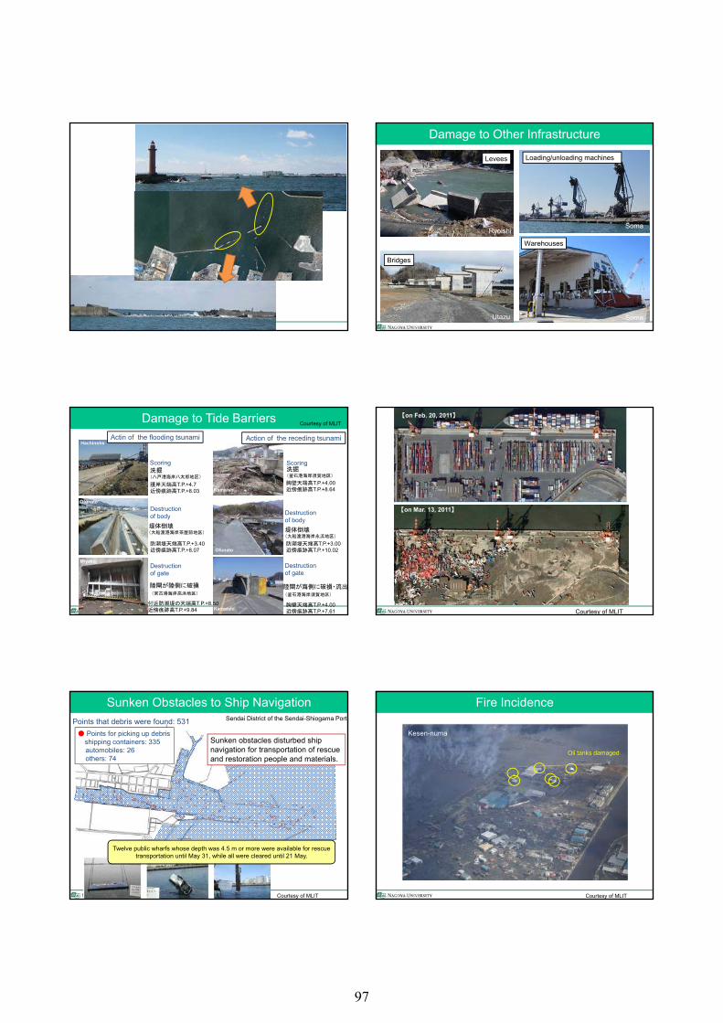
Damage to Other Infrastructure
Ryoishi
Soma
Soma
Levees Loading/unloading machines
Warehouses
Utazu
Bridges
堤体倒壊(大船渡港海岸茶屋前地区) 堤体倒壊
(大船渡港海岸永浜地区)
洗掘(釜石港海岸須賀地区)
洗掘(八戸港海岸八太郎地区)
陸閘が海側に破損・流出(釜石港海岸須賀地区)
陸閘が陸側に破損(宮古港海岸高浜地区)
Damage to Tide Barriers
護岸天端高T.P.+4.7近傍痕跡高T.P.+8.03
胸壁天端高T.P.+4.00近傍痕跡高T.P.+8.64
防潮堤天端高T.P.+3.40近傍痕跡高T.P.+8.07
防潮堤天端高T.P.+3.00近傍痕跡高T.P.+10.02
付近防潮堤の天端高T.P.+8.50近傍痕跡高T.P.+9.84
胸壁天端高T.P.+4.00近傍痕跡高T.P.+7.61
Actin of the flooding tsunami Action of the receding tsunami
Scoring Scoring
Destruction of body
Destruction of body
Destruction of gate
Destruction of gate
Hachinohe
Ofunato
Miyako
Kamaishi
Ofunato
Kamaishi
Courtesy of MLIT
【on Mar. 13, 2011】
【on Feb. 20, 2011】
Courtesy of MLIT
Sunken Obstacles to Ship NavigationSendai District of the Sendai-Shiogama Port
Twelve public wharfs whose depth was 4.5 m or more were available for rescue transportation until May 31, while all were cleared until 21 May.
Points that debris were found: 531
● Points for picking up debrisshipping containers: 335automobiles: 26others: 74
Courtesy of MLIT
Sunken obstacles disturbed ship navigation for transportation of rescue and restoration people and materials.
Courtesy of MLIT
Fire Incidence
Kesen-numa
Oil tanks damaged
97
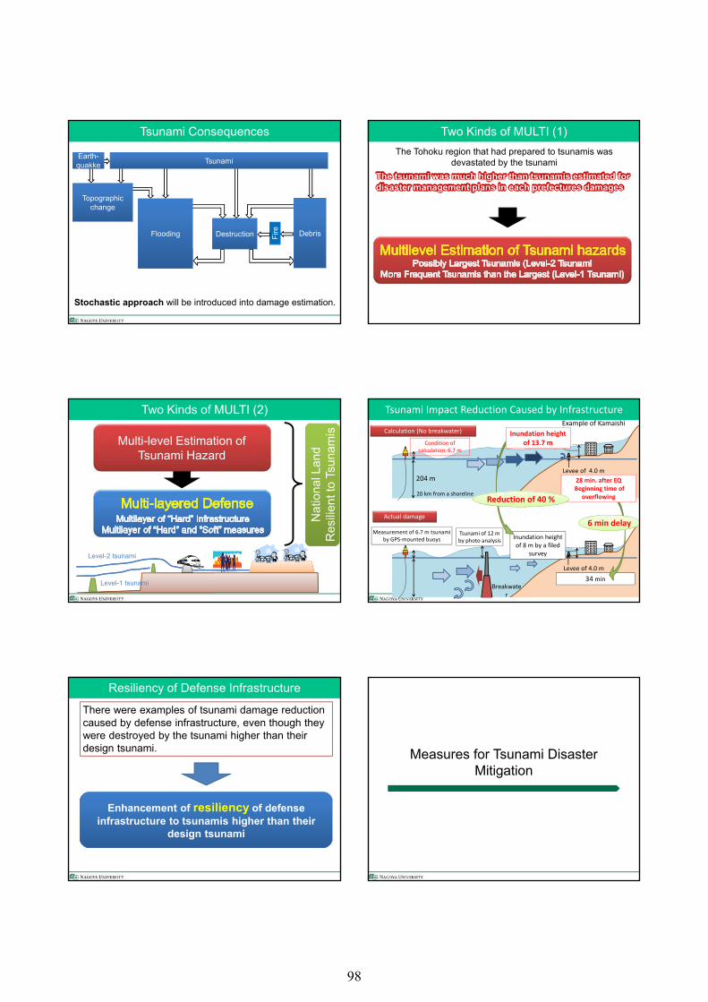
Tsunami Consequences
Fire
Topographic change
Flooding
TsunamiqEarth-quakke
Stochastic approach will be introduced into damage estimation.
Destruction Debris
陸前高田市 高田松原
宮古市
Two Kinds of MULTI (1)
The Tohoku region that had prepared to tsunamis was devastated by the tsunami
The tsunami was much higher than tsunamis estimated for disaster management plans in each prefectures damages
Two Kinds of MULTI (2)
Level-1 tsunami
Level-2 tsunami
Multi-level Estimation of Tsunami Hazard
Nat
iona
l Lan
d R
esili
ent t
o Ts
unam
is
Tsunami Impact Reduction Caused by Infrastructure
Measurement of 6.7 m tsunami by GPS‐mounted buoys
Calculation (No breakwater)
20 km from a shoreline
Levee of 4.0 m
Breakwater
Tsunami of 12 m by photo analysis
Actual damage
Condition of calculation: 6.7 m
Levee of 4.0 m
34 min
6 6 min delay
28 min. after EQBeginning time of
overflowing
Inundation height of 8 m by a filed
survey
Inundation height of 13.7 m
Reduction of 40 %Reduction of 40 %
204 m
Example of Kamaishi
Resiliency of Defense Infrastructure
There were examples of tsunami damage reduction caused by defense infrastructure, even though they were destroyed by the tsunami higher than their design tsunami.
Enhancement of resiliency of defense infrastructure to tsunamis higher than their
design tsunami
Measures for Tsunami Disaster Mitigation
98
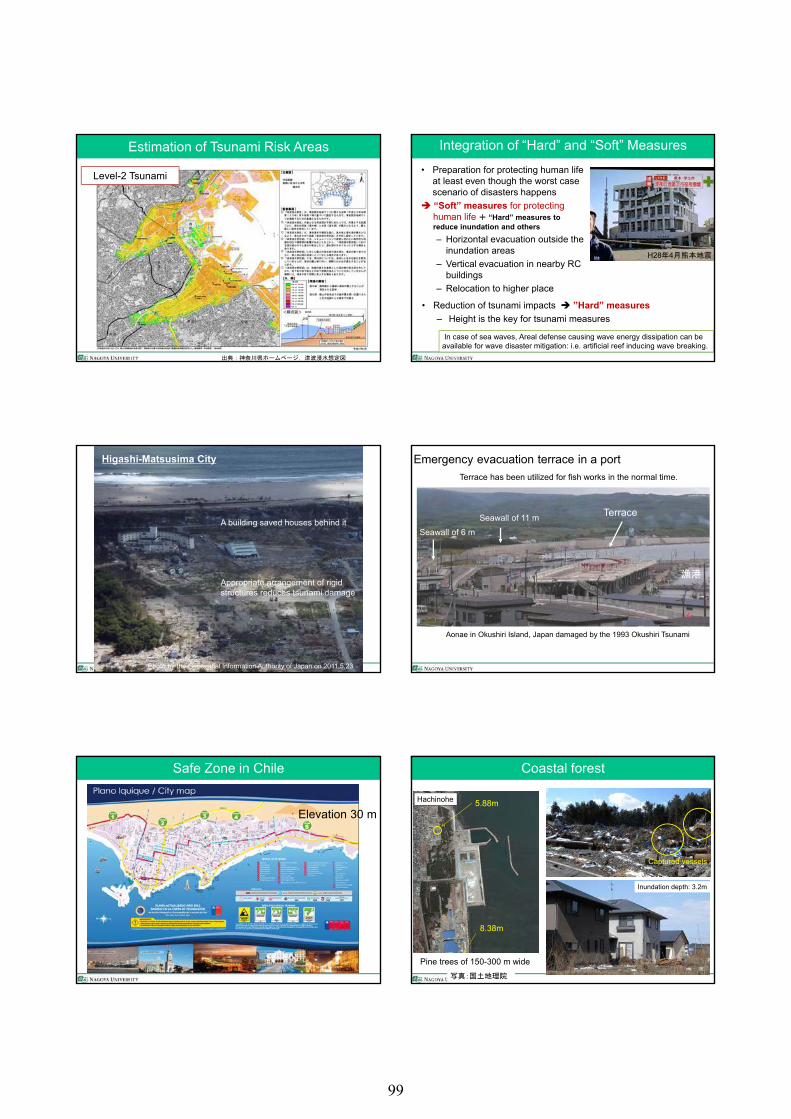
Estimation of Tsunami Risk Areas
出典:神奈川県ホームページ,津波浸水想定図
Level-2 Tsunami
Integration of “Hard” and “Soft” Measures
• Preparation for protecting human life at least even though the worst case scenario of disasters happens
“Soft” measures for protecting human life + “Hard” measures to reduce inundation and others
– Horizontal evacuation outside the inundation areas
– Vertical evacuation in nearby RC buildings
– Relocation to higher place
H28年4月熊本地震
• Reduction of tsunami impacts ”Hard” measures
– Height is the key for tsunami measures
In case of sea waves, Areal defense causing wave energy dissipation can be available for wave disaster mitigation: i.e. artificial reef inducing wave breaking.
Photo by the Geospatial Information Authority of Japan on 2011.5.23
Higashi-Matsusima City
A building saved houses behind it
Appropriate arrangement of rigid structures reduces tsunami damage
TerraceSeawall of 11 m
Seawall of 6 m
漁港
Aonae in Okushiri Island, Japan damaged by the 1993 Okushiri Tsunami
Emergency evacuation terrace in a port
Terrace has been utilized for fish works in the normal time.
Safe Zone in Chile
Elevation 30 m
Coastal forest
写真:国土地理院
Inundation depth: 3.2m
Pine trees of 150-300 m wide
8.38m
5.88mHachinohe
Captured vessels
99
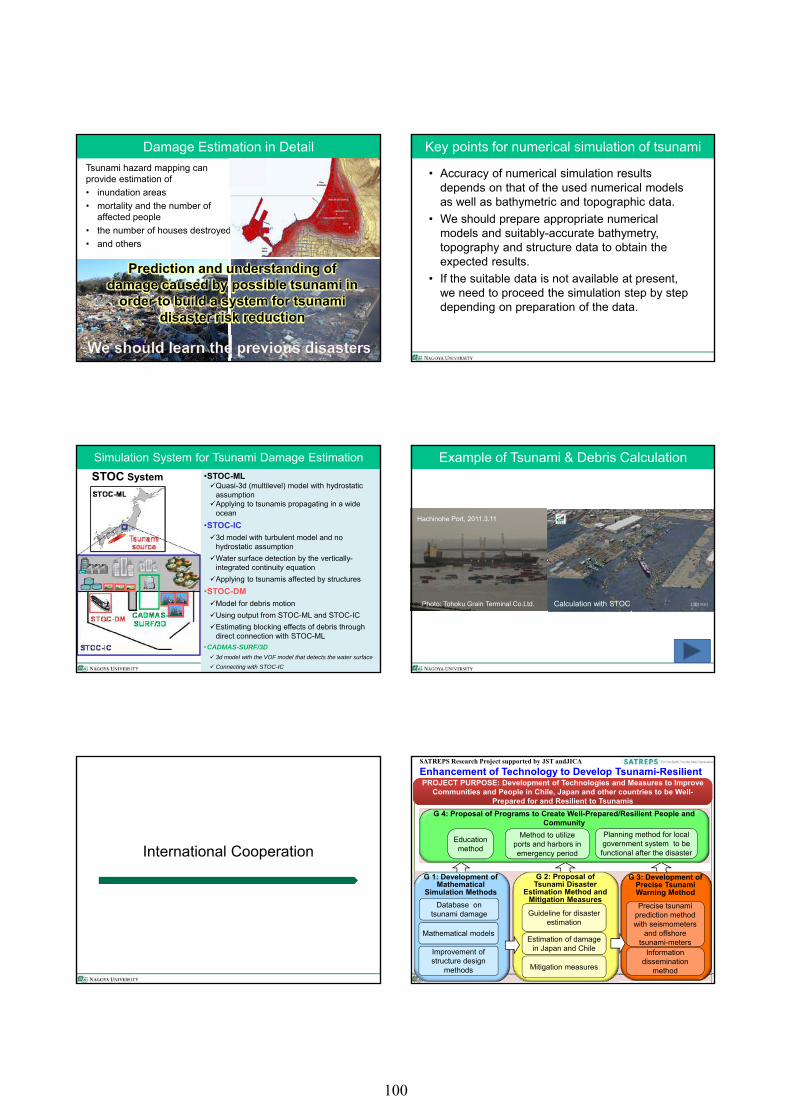
Damage Estimation in Detail
Tsunami hazard mapping can provide estimation of
• inundation areas
• mortality and the number of affected people
• the number of houses destroyed,
• and others
Prediction and understanding of damage caused by possible tsunami in
order to build a system for tsunami disaster risk reduction
Key points for numerical simulation of tsunami
• Accuracy of numerical simulation results depends on that of the used numerical models as well as bathymetric and topographic data.
• We should prepare appropriate numerical models and suitably-accurate bathymetry, topography and structure data to obtain the expected results.
• If the suitable data is not available at present, we need to proceed the simulation step by step depending on preparation of the data.
Simulation System for Tsunami Damage Estimation
•STOC-MLQuasi-3d (multilevel) model with hydrostatic
assumptionApplying to tsunamis propagating in a wide
ocean
•STOC-IC
3d model with turbulent model and no hydrostatic assumption
Water surface detection by the vertically-integrated continuity equation
Applying to tsunamis affected by structures
•STOC-DM
Model for debris motion
Using output from STOC-ML and STOC-IC
Estimating blocking effects of debris through direct connection with STOC-ML
•CADMAS-SURF/3D
3d model with the VOF model that detects the water surface
Connecting with STOC-IC
STOC System
Example of Tsunami & Debris Calculation
Photo: Tohoku Grain Terminal Co.Ltd.
Hachinohe Port, 2011.3.11
Calculation with STOC
International Cooperation
SATREPS Research Project supported by JST andJICA
Enhancement of Technology to Develop Tsunami-Resilient Community
Database on tsunami damage
Mathematical models
Guideline for disaster estimation
Precise tsunami prediction method with seismometers
and offshore tsunami-metersEstimation of damage
in Japan and Chile Information dissemination
method
p
PROJECT PURPOSE: Development of Technologies and Measures to Improve Communities and People in Chile, Japan and other countries to be Well-
Prepared for and Resilient to Tsunamis
Method to utilize ports and harbors in emergency period
Planning method for local government system to be functional after the disaster
Education method
Improvement of structure design
methods Mitigation measures
G 1: Development of Mathematical
Simulation Methods
G 4: Proposal of Programs to Create Well-Prepared/Resilient People and Community
G 2: Proposal of Tsunami Disaster
Estimation Method and Mitigation Measures
G 3: Development of Precise Tsunami Warning Method
100
Building National Resilience to Disasters
High Damage Cost in Capital: Japan Case
• Estimated damage in the 2011 Tohoku event
– 154 billion US$ approx.
– Death toll: 20,000
– Complete destroyed buildings: 130,000
• Possible earthquake disaster in the Capital
– 431 billion US$ approx.
– Death toll: 23,000 max.
– Complete destroyed buildings: 610,000 max.
If an big incident occurs in the Capital area that population and assets are concentrated in Japan, its disaster can become severe
Building National Resiliency: Japan Case
• Aging population and birthrate declining– Lack of persons who are responsible for taking care of handicap
persons, and working rehabilitation and restoration activities Necessary for keeping and increasing population of productive age
• Building environment to easily live as well as to be safety and security
• Balance of natural hazard resiliency, industry development, and sustainable environment– Natural disasters, society and economy, and environment highly
depending on local characteristics
National Land Use Design for Building Resiliency to Tsunamis
Consensus building
Consensus building
Estimation of tsunami damage
Sustainable development
Happy Unhappy
Yes No
Measures• Relocation to a high place• Construction of a tall defense structure• Construction of a low defense structure
No
Yes30 or 50 years later
Measure /Residual risk
Nature Economy
Society
Convenience
DevelopmentEnvironmentalImpact
Summary
Summary
• Strengthening of critical infrastructures including defense structures, transportation systems, lifelines, schools, hospitals to build national land resilient to natural disasters such as tsunamis.
• Multi-level estimation of hazards to build integrated and inclusive measures for enhancement of resiliency of people, society and economy.
• Multi-layered defense system to protect people from unexpected tsunamis
• Understanding of geographical and social vulnerability, and previous disasters in the area and in the world.
101

102
L8: Tidal Flat Conservation Hiromi YAMASHITA, PhD. (Ritsumeikan Asia Pacific University: APU, Japan) Abstract
A tidal flat is a curious place where mud appears in shallow areas of coastal water when the tide is low. It supports not only an immense variety of wildlife, but also has an economic value, including providing a source of food, water purification, erosion control, and reducing damage from tsunamis. Among conservationists, tidal flats are regarded as one of the most important areas to conserve for the health of the wider coastal and oceanic environments. International convention documents, such as those produced by Ramsar, emphasize this (e.g. Ramsar Convention Secretariat 2008).
In this context, cities within 60 km of the sea are growing. Some 60 % of the world’s population lives within 60 km of the sea and current trends suggest that this figure will rise to 75 % by the year 2025. Three quarters of the world’s megacities are coastal, even though coastal regions harbour many of the Earth’s most diverse, complex, and productive ecosystems (UNESCO 1997). Many of the city developments in coastal areas have utilized tidal flats to expand available land to use for living, transportation, and infrastructure. At the present time, in many countries more than half of the population lives in a coastal zone, a percentage that is increasing.
Although the ecological importance of wetlands and tidal flats has been widely communicated in recent years (e.g. Smardon 2009), they are still under great pressure from urban and coastal development projects in Japan and abroad. In Japan, between the 1940s and 1980s nearly 40 % of the natural tidal flats were lost through reclamation, and currently it is said to be 50 % or more (e.g. Baba et al. 2003).
There is little detailed study on how wetlands and tidal flats are perceived by people who have not had direct contact with them. However, it is well observed by wetland conservationists in many countries that wetlands and tidal flats have often been referred to as “wastelands” by the general public.
This course looks at the importance of tidal flats; existing tidal flat management arrangements and issues for the conservation and sustainable use of the areas; and how the ecological importance of tidal flat can be communicated effectively.
103

104
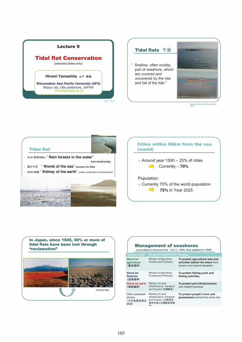
1
������� �
�� �� ������������������������������� �
Hiromi Yamashita
Ritsumeikan Asia Pacific University (APU) Beppu city, Oita prefecture, JAPAN
������������ ��
2016.12.08.
�� �� ���
“ Shallow, often muddy, part of seashore, which are covered and uncovered by the rise and fall of the tide ”
Toyohashi Museum of Natural History 2010
�� �� ��
� “ Rain forests in the water” (rich biodiversity)
� “ Womb of the sea” (nursery for fish)
� “ Kidney of the earth” (water purification mechanisms)
�������������������������������� ���
� Around year 1500 – 25% of cities Currently – 70%
Population� Currently 70% of the world population
75% in Year 2025
�������� ������!�"# �#�$��������������� �� ���������%���� ���������&��“reclamation”
Isahaya Bay
'���&��������������������������&����(�������� �� !�#� ����������������!����
Types of coasts Management responsibility Purpose
Shore for agriculture
Ministry of Agriculture, Forestry and Fisheries
To protect agricultural land and activities behind the shore from erosion and natural disasters
Shore for fisheries
Ministry of Agriculture, Forestry and Fisheries
To protect fishing ports and fishing activities
Shore for ports Ministry of Land, Infrastructure, Transport and Tourism
To protect port infrastructures and related business
Other protected shores
Ministry of Land, Infrastructure, Transport and Tourism
To protect people’s lives and possessions behind the shore line
105
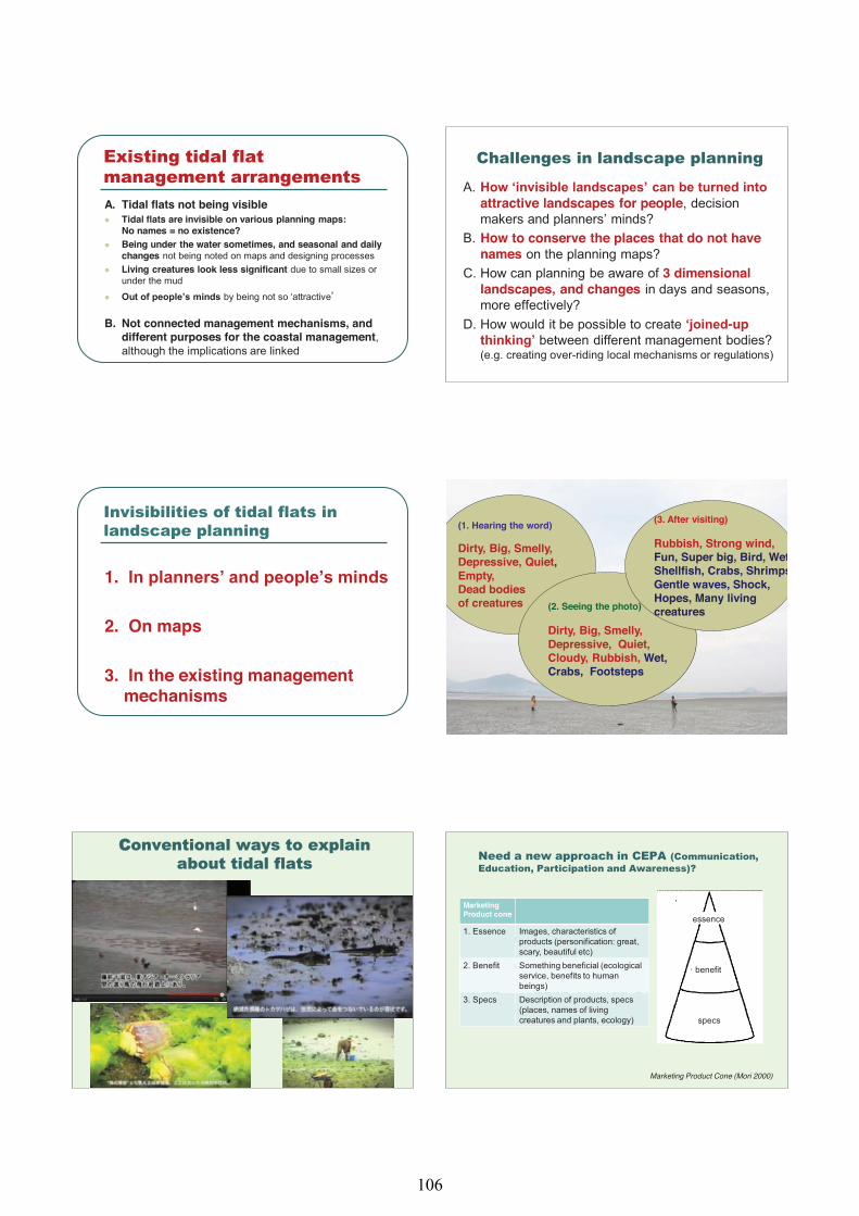
2
)*���&���� �� �������&�����������&������A. Tidal flats not being visible� Tidal flats are invisible on various planning maps:
No names = no existence? � Being under the water sometimes, and seasonal and daily
changes not being noted on maps and designing processes� Living creatures look less significant due to small sizes or
under the mud
� Out of people’s minds by being not so ‘attractive’
B. Not connected management mechanisms, and different purposes for the coastal management, although the implications are linked
��� ��&����� ���������� ����&�
A. How ‘invisible landscapes’ can be turned into attractive landscapes for people, decision makers and planners’ minds?
B. How to conserve the places that do not have names on the planning maps?
C. How can planning be aware of 3 dimensional landscapes, and changes in days and seasons, more effectively?
D. How would it be possible to create ‘joined-up thinking’ between different management bodies? (e.g. creating over-riding local mechanisms or regulations)
����% ���������� �� ������ ���������� ����&
1. In planners’ and people’s minds
2. On maps
3. In the existing management mechanisms
(1. Hearing the word)
Dirty, Big, Smelly,Depressive, Quiet, Empty, Dead bodies of creatures (2. Seeing the photo)
Dirty, Big, Smelly, Depressive, Quiet, Cloudy, Rubbish, Wet, Crabs, Footsteps
(3. After visiting)
Rubbish, Strong wind, Fun, Super big, Bird, WetShellfish, Crabs, ShrimpsGentle waves, Shock, Hopes, Many living creatures
����������� ���+������*� ����%������� �� ��� ,����������������������)-.������������� �
)������� �-��������������.���������/�
Marketing Product Cone (Mori 2000)
MarketingProduct cone
1. Essence Images, characteristics of products (personification: great, scary, beautiful etc)
2. Benefit Something beneficial (ecological service, benefits to human beings)
3. Specs Description of products, specs (places, names of living creatures and plants, ecology)
essence
benefit
specs
106
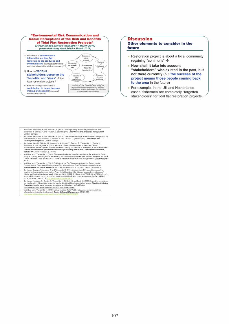
3
“Environmental Risk Communication and (��� �-�����������������1�������2�������
of Tidal Flat Restoration Projects” �3�+��������������4���5�.�� �6�!!�7�'�����6�!"��
��*�����������+�.�� �6�!#�7�'�����6�!��
���������� � �������� ��� ����� ������������������������������������������ ����������������������������������
������������������������
Restoration Projects
(������������� �
����������������������������
�������������
�������
��������������� ������ �����
�������������� ��������
�����
�������������������
����� �����
1) What kinds of environmental information on tidal flat restorations are produced and communicated by project contractors and other stakeholders in the community?
2) How do various stakeholders perceive the ‘benefits’ and ‘risks’ of their local restoration projects?
3) How the findings could make a contribution to future decision making and support for coastal wetland restorations?
8�������9������ ������������������������������
� Restoration project is about a local community regaining “commons” �
� How shall it take into account “stakeholders” who existed in the past, but not there currently (but the success of the project means those people coming back to the area in the future)
� For example, in the UK and Netherlands cases, fishermen are completely “forgotten stakeholders” for tidal flat restoration projects.
� Joint work. Yamashita, H. and Yasufuku, T. (2016) Coastal planning: Biodiversity conservation and ownership, in Shimizu, H. and Takatori, C. (2016 in print) Labor forces and landscape management. London: Springer.
� Joint work. Yamashita, H. and Yasufuku, T. (2016) Coastal area landscape: Environmental changes and the characteristics of labor activities, in Shimizu, H. and Takatori, C. (2016 in print) Labor forces and landscape management. London: Springer.
� Joint work. Kato, H., Shimizu, H., Kawamura, N., Hirano, Y., Tashiro, T., Yamashita, H., Tomita, K., Tomiyoshi, M. and Hagihara, K. (2014) A Prospect Toward Establishment of Basic and Clinical Environmental Studies by ORT (On-Site Research Training), in Shimizu, H. Murayama, A. (eds) Basic and Clinical Environmental Approaches in Landscape Planning. Urban and Landscape Perspectives, Volume 17. London: Springer. p.133-143
� Individual work. Yamashita, H. (2016) ‘Discourse of risks and benefits towards tidal flat restoration: Case study of “opening a water gate” of Isahaya Bay land reclamation in Ariake Sea, Wetland Research. 2016 6 1
3-17� Individual work. Yamashita, H. (2015) Problems of the ‘Fact’-Focused Approach in Environmental
Communication: Examples of Environmental Risk Information on Tidal Flat Developments in Japan. Environmental Education Research, Vol.21(4), pp.586-611. DOI: 10.1080/13504622.2014.940281
� Joint work. Ikegawa, T. Aoyama, T. and Yamashita, H. (2014, in Japanese) ‘Ethnographic research for creating environmental communication: From the field work on tidal flats and surrounding environment’, “Media and Society [Media to shakai]”, Vol.6, pp.39-53. 2014
Vol.6, pp.39-53. 2014 3 http://hdl.handle.net/2237/19815� Joint work. Hockings, C., Cooke, S., Yamashita, H. McGinty, S. and Bowl, M. (2009) ‘I’m neither entertaining
nor charismatic…’ Negotiating university teacher identity within diverse student groups. Teaching in Higher Education, Special Issue: purposes, knowledge and identities, 14(5):470-483. http://www.tandfonline.com/doi/abs/10.1080/13562510903186642
� Individual work. Yamashita, H. (2009) Making Invisible Risks Visible: Education, environmental risk information and coastal development. Ocean & Coastal Management, 52:327-335.http://www.sciencedirect.com/science/article/pii/S0964569109000258
107

108
E1: Analysis of satellite data for monitoring and assessment for coastal eutrophication Genki Terauchi (NOWPAP CEARAC) Abstract Marine eutrophication has recently become a concern for all the world’s oceans. There are over 415 areas worldwide identified as manifesting symptoms of eutrophication. Eutrophication causes deterioration of the coastal environment and often leads to the formation of harmful algal blooms and depletion of bottom oxygen, which may subsequently induce fish kills and/or ecosystem damage. Eutrophication was originally used in limnology to describe the natural process of nutrient enrichment concomitant with the aging of lakes and ponds. However, it is known that humans, through various activities, can greatly accelerate this natural process by increasing nutrient input into bodies of water. Northwest Pacific region, which includes parts of northeast China, Japan, Korea and southeast Russia, is one of the most densely populated areas of the world, and its coastal systems are under pressure from human activities. In deed, a significant number of red tides and hypoxic conditions have been reported in coastal waters - possibly due to anthropogenic influences such as extensive chemical fertilizer use and sewage effluent.
In this training course, case studies of use of remotely sensed chlorophyll-a concentration (satellite Chl-a) in Toyama Bay, Japan will be introduced. Preparing a consistent long-term time series satellite Chl-a data sets and a methodology for quality assurance processes will be included. Interannual and seasonal variability of satellite Chl-a and its changes associated with fresh water discharge will then be discussed. Use of Google Earth Engine, a cloud-computing platform for processing satellite imagery, for detection of changes in coastal habitats will also be introduced.
109

110
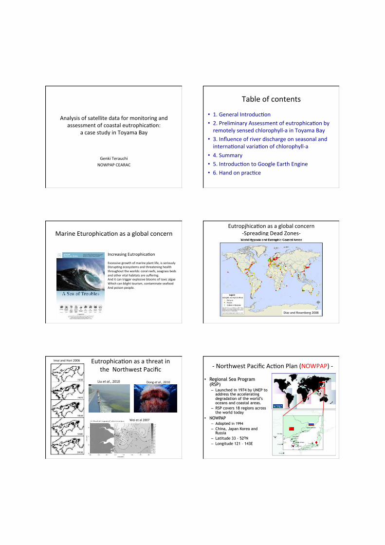
Analysisofsatellitedataformonitoringandassessmentofcoastaleutrophica5on:
acasestudyinToyamaBay
GenkiTerauchiNOWPAPCEARAC
Tableofcontents
• 1.GeneralIntroduc5on• 2.PreliminaryAssessmentofeutrophica5onbyremotelysensedchlorophyll-ainToyamaBay
• 3.Influenceofriverdischargeonseasonalandinterna5onalvaria5onofchlorophyll-a
• 4.Summary• 5.Introduc5ontoGoogleEarthEngine• 6.Handonprac5ce
MarineEturophica5onasaglobalconcern
IncreasingEutrophica5onExcessivegrowthofmarineplantlife,isseriouslyDisrup5ngecosystemsandthreateninghealththroughouttheworlds:coralreefs,seagrassbedsandothervitalhabitatsaresuffering.AnditcantriggerexplosivebloomsoftoxicalgaeWhichcanblighttourism,contaminateseafoodAndpoisonpeople.
Eutropjhica5onasaglobalconcern-SpreadingDeadZones-
DiazandRosenberg2008
ImaiandHori2006
Weietal2007
Eutrophica5onasathreatintheNorthwestPacific
Liuetal.,2010 Dongetal.,2010
-NorthwestPacificAc5onPlan(NOWPAP)-
• Regional Sea Program (RSP) – Launched in 1974 by UNEP to
address the accelerating degradation of the world’s oceans and coastal areas.
– RSP covers 18 regions across the world today
• NOWPAP – Adopted in 1994 – China, Japan Korea and
Russia – Latitude 33 - 52ON – Longitude 121 – 143E
jimu
タイプライターテキスト
111
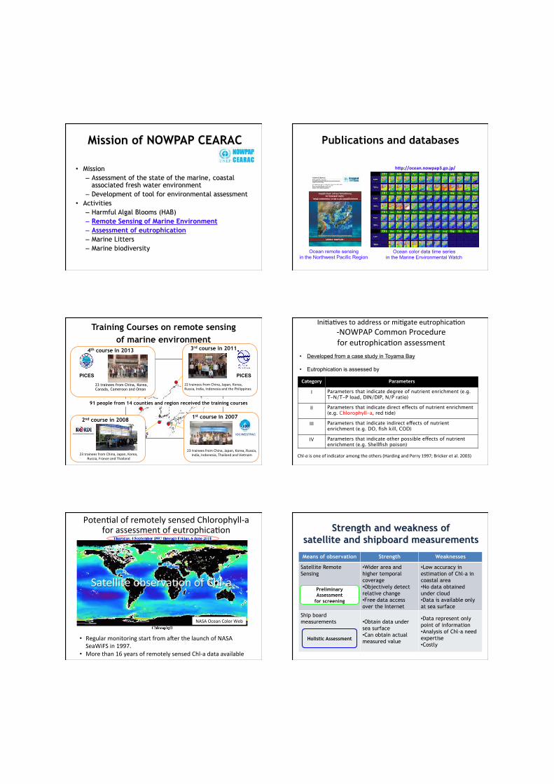
Mission of NOWPAP CEARAC�
• Mission – Assessment of the state of the marine, coastal
associated fresh water environment – Development of tool for environmental assessment
• Activities – Harmful Algal Blooms (HAB) – Remote Sensing of Marine Environment – Assessment of eutrophication – Marine Litters – Marine biodiversity
Publications and databases�
Ocean remote sensing in the Northwest Pacific Region
Ocean color data time series in the Marine Environmental Watch
h"p://ocean.nowpap3.go.jp/
Training Courses on remote sensing of marine environment
IOC/WESTPAC
1st course in 2007
3rd course in 2011
2nd course in 2008
4th course in 2013
23 trainees from China, Korea, Canada, Cameroon and Oman
23traineesfromChina,Japan,Korea,Russia,India,Indonesia,ThailandandVietnam
22traineesfromChina,Japan,Korea,Russia,India,IndonesiaandthePhilippines
23traineesfromChina,Japan,Korea,Russia,FranceandThailand
91 people from 14 counties and region received the training courses
PICES PICES
Ini5a5vestoaddressormi5gateeutrophica5on-NOWPAPCommonProcedureforeutrophica5onassessment
• Developed from a case study in Toyama Bay
• Eutrophication is assessed by
Category Parameters
I Parameters that indicate degree of nutrient enrichment (e.g. T-N/T-P load, DIN/DIP, N/P ratio)
II Parameters that indicate direct effects of nutrient enrichment (e.g. Chlorophyll-a, red tide)
III Parameters that indicate indirect effects of nutrient enrichment (e.g. DO, fish kill, COD)
IV Parameters that indicate other possible effects of nutrient enrichment (e.g. Shellfish poison)
Chl-aisoneofindicatoramongtheothers(HardingandPerry1997;Brickeretal.2003)
Satelliteobserva5onofChl-a
NASAOceanColorWeb
• RegularmonitoringstartfromaferthelaunchofNASASeaWiFSin1997.
• Morethan16yearsofremotelysensedChl-adataavailable
Poten5alofremotelysensedChlorophyll-aforassessmentofeutrophica5on Strength and weakness of
satellite and shipboard measurements�
Means of observation� Strength� Weaknesses�
Satellite Remote Sensing�
• Wider area and higher temporal coverage • Objectively detect relative change • Free data access over the Internet
• Low accuracy in estimation of Chl-a in coastal area • No data obtained under cloud • Data is available only at sea surface�
Ship board measurements� • Obtain data under
sea surface • Can obtain actual measured value
• Data represent only point of information • Analysis of Chl-a need expertise • Costly�
Preliminary Assessment
for screening
Holistic Assessment
jimu
タイプライターテキスト
112
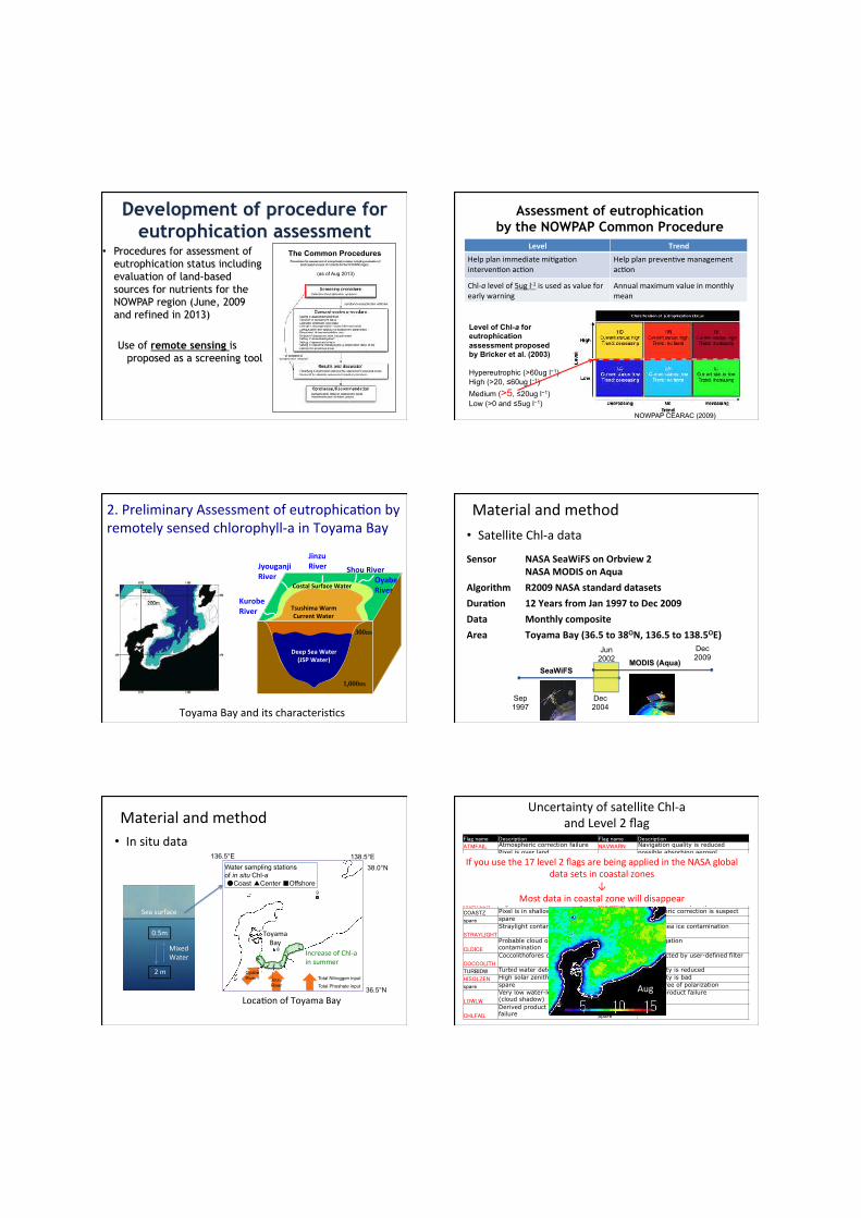
Development of procedure for eutrophication assessment�
• Procedures for assessment of eutrophication status including evaluation of land-based sources for nutrients for the NOWPAP region (June, 2009 and refined in 2013)
Use of remote sensing is proposed as a screening tool
The Common Procedures
(as of Aug 2013)
Assessment of eutrophication by the NOWPAP Common Procedure�
NOWPAP CEARAC (2009)
Level of Chl-a for eutrophication assessment proposed by Bricker et al. (2003) Hypereutrophic (>60ug l−1) High (>20, ≤60ug l−1) Medium (>5, ≤20ug l−1) Low (>0 and ≤5ug l−1)
Level TrendHelpplanimmediatemi5ga5oninterven5onac5on
Helpplanpreven5vemanagementac5on
Chl-alevelof5ugl-1isusedasvalueforearlywarning
Annualmaximumvalueinmonthlymean
2.PreliminaryAssessmentofeutrophica5onbyremotelysensedchlorophyll-ainToyamaBay
ToyamaBayanditscharacteris5cs
CostalSurfaceWater
TsushimaWarmCurrentWater
DeepSeaWater(JSPWater)
300m
KurobeRiver
JyouganjiRiver
JinzuRiver ShouRiver
OyabeRiver
1,000m
Materialandmethod• SatelliteChl-adataSensor NASASeaWiFSonOrbview2
NASAMODISonAquaAlgorithm R2009NASAstandarddatasetsDuraTon 12YearsfromJan1997toDec2009Data MonthlycompositeArea ToyamaBay(36.5to38ON,136.5to138.5OE)
Sep 1997
MODIS (Aqua)
Jun 2002
Dec 2004
SeaWiFS
Dec 2009
Materialandmethod
36.5°N
38.0°N
136.5°E 138.5°E
ToyamaBay
1 2 3 4 5
6 7
Water sampling stations of in situ Chl-a
Coast Center Offshore
8
9
ToyamaBay
Loca5onofToyamaBay
0.5m
2m
Seasurface
IncreaseofChl-ainsummer
Oyabe River Jinzu
River Total Nitroggen input
MixedWater
Total Phoshate input
• Insitudata
UncertaintyofsatelliteChl-aandLevel2flag
Atmospheric correction failure Navigation quality is reduced Pixel is over land possible absorbing aerosol
(disabled) One or more product warnings spare High sun glint Aerosol iterations exceeded max
Observed radiance very high or saturated
Moderate sun glint contamination
High sensor view zenith angle Derived product quality is reduced Pixel is in shallow water Atmospheric correction is suspect spare spare Straylight contamination is likely Possible sea ice contamination
Probable cloud or ice contamination
Bad navigation
Coccolithofores detected Pixel rejected by user-defined filter
Turbid water detected SST quality is reduced High solar zenith SST quality is bad spare High degree of polarization Very low water-leaving radiance (cloud shadow)
Derived product failure
Derived product algorithm failure
spare
Ifyouusethe17level2flagsarebeingappliedintheNASAglobaldatasetsincoastalzones
↓Mostdataincoastalzonewilldisappear
Aug
jimu
タイプライターテキスト
113
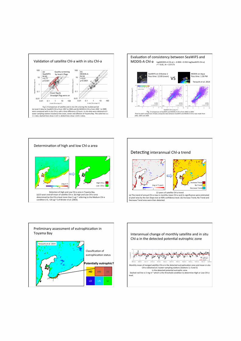
In situ Chl-a (mg m-3)
Sea
WiF
S C
hl-a
(mg
m-3
)
MO
DIS
-A C
hl-a
(mg
m-3
)
0.01
0.1
1
10
100
0.01 0.1 1 10 100
(a) SeaWiFS N=42 r=0.77 p<0.001
0.01
0.1
1
10
100
0.01 0.1 1 10 100
(b) MODIS-A N=34 r=0.81 p<0.0001
In situ Chl-a (mg m-3)
Valida5onofsatelliteChl-awithinsituChl-a
Fig2.3ComparisonofsatelliteandinsituChl-aduringthestudiedperiod(a)Level-2dataforSeaWiFSChl-afrom1997to2004and(b)MODIS-AChl-afrom2002 to2009werecomparedwithinsituChl-a,witha5medifference≤3hours.Insitudatawereobtainedat9watersamplingsta5onslocatedatthecoast,centerandoffshoreofToyamaBay.Thesolidlineisa1:1ra5o;dashedlinesshow1:2/2:1;dokedlinesshow1:3/3:1ra5os.
Qualityscreeningbylevel-2flags
Coastflag&Straylightflagwereon
Fig. 3 ComparisonofSeaWiFSandMODIS-AChl-afrom2002to2004.Pixel-to-pixelcomparisonofdailycompositedatabetweenSeaWiFSandMODIS-AChl-awasmadefrom2002,2003and2004.
SeaWiFS Chl-a (mg m-3)
MO
DIS
-A C
hl-a
(mg
m-3
)
����
���
�
��
���
��� � �� ���
�������������������
����
���
�
��
���
���� ��� � �� ���
����
���
�
��
���
���� ��� � �� ���
2002 2003 2004
Numberofplots
N=30837R2=0.807
Y=-0.079+0.925*X
N=45505R2=0.792
Y=-0.061+0.946*X
N=60831R2=0.818
Y=0.019+1.136*X
Evalua5onofconsistencybetweenSeaWiFSandMODIS-AChl-a
SeaWiFSonOrbview-2Pass5me:12:00(noon)
MODISonAquaPass5me:1:30PMVS
log(MODIS-AChl-a)=-0.900+0.932log(SeaWiFSChl-a)r2=0.81,N=137173
Terauchietal.2014
HighChl-a�LowChl-a�
(mgm-3)
Determina5onofhighandlowChl-aarea
Detec5onofHighandLowChl-aareainToyamaBay.(a)13-yearsoverallmeanofsatelliteChl-a.(b)HighandLowChl-aareadeterminedbytheChl-alevelmorethan5ugl-1referringtotheMediumChl-acondi5on(>5,<20ugl-1)ofBrickeretal.(2003).
12-yearsofsatelliteChl-atrend.(a)ThetrendofannualChl-amaxinmonthlymeanChl-aanditssignificancewerees5matedatpixelwisebytheSenSlopetestat90%confidencelevel.(b)IncreaseTrend,NoTrendandDecreaseTrendareawerethendetected.
IncreaseTrend�NoTrend�
DecreaseTrend�(mgm-3/year)
Detec5nginterannualChl-atrend
Preliminaryassessmentofeutrophica5oninToyamaBay
(mgm-3)(mgm-3/year)
HD HN HI
LD LN LI
Potentially eutrophic?
Classifica5onofeutrophica5onstatus
Terauchietal.2014
InterannualchangeofmonthlysatelliteandinsituChl-ainthedetectedpoten5aleutrophiczone
MonthlymeanofmergedsatelliteChl-ainthedetectedeutrophica5onzoneandmeaninsituChl-aobtainedat3water-samplingsta5ons(Sta5ons3,4and5)
inthedetectedpoten5aleutrophiczone.Dashedredlineis5mgm-3whichisthethresholdcondi5ontodetermineHighorLowChl-alevel.
jimu
タイプライターテキスト
114
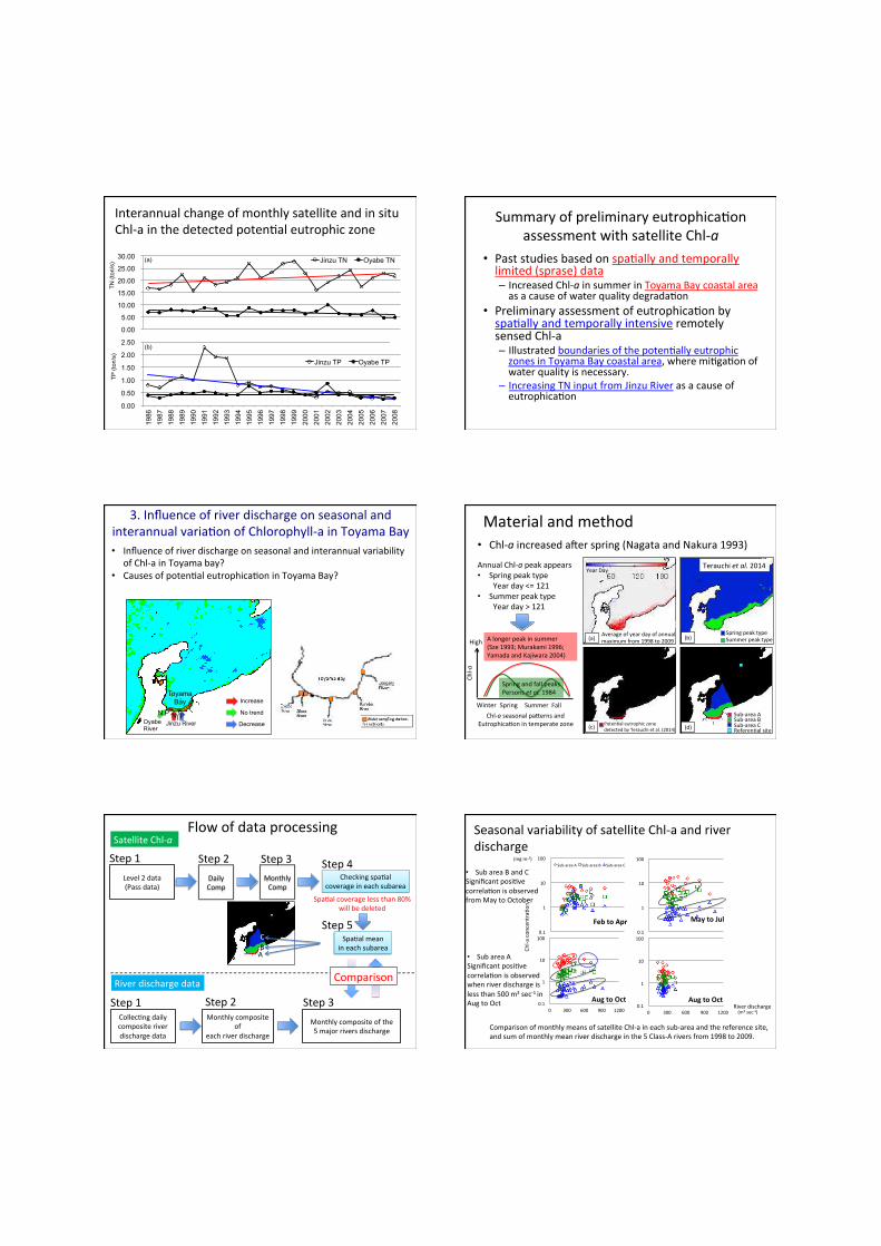
0.00
5.00
10.00
15.00
20.00
25.00
30.00 Jinzu TN Oyabe TN (a)
0.00
0.50
1.00
1.50
2.00
2.50
1986
19
87
1988
19
89
1990
19
91
1992
19
93
1994
19
95
1996
19
97
1998
19
99
2000
20
01
2002
20
03
2004
20
05
2006
20
07
2008
Jinzu TP Oyabe TP
(b)
TN (t
on/s
)TP
(ton
/s)
InterannualchangeofmonthlysatelliteandinsituChl-ainthedetectedpoten5aleutrophiczone
Summaryofpreliminaryeutrophica5onassessmentwithsatelliteChl-a�
• Paststudiesbasedonspa5allyandtemporallylimited(sprase)data– IncreasedChl-ainsummerinToyamaBaycoastalareaasacauseofwaterqualitydegrada5on
• Preliminaryassessmentofeutrophica5onbyspa5allyandtemporallyintensiveremotelysensedChl-a– Illustratedboundariesofthepoten5allyeutrophiczonesinToyamaBaycoastalarea,wheremi5ga5onofwaterqualityisnecessary.
– IncreasingTNinputfromJinzuRiverasacauseofeutrophica5on
3.Influenceofriverdischargeonseasonalandinterannualvaria5onofChlorophyll-ainToyamaBay• Influenceofriverdischargeonseasonalandinterannualvariability
ofChl-ainToyamabay?• Causesofpoten5aleutrophica5oninToyamaBay?
Jinzu River Oyabe River
N P N,P Decrease
Increase
No trend
Toyama Bay
(a)
(a)SpringpeaktypeSummerpeaktype
Averageofyeardayofannualmaximumfrom1998to2009 (b)
(d)
Sub-areaASub-areaBSub-areaCReferen5alsite
Poten5aleutrophiczonedetectedbyTerauchietal.(2014)(c)
YearDay
Materialandmethod• Chl-aincreasedaferspring(NagataandNakura1993)AnnualChl-apeakappears• Springpeaktype
Yearday<=121• Summerpeaktype
Yearday>121
Alongerpeakinsummer(Sze1993;Murakami1996;YamadaandKajiwara2004)
Summer FallWinter
Chl-a�
Chl-aseasonalpakernsandEutrophica5onintemperatezone
SpringandfallpeaksPersonsetal.1984
High
Spring
Terauchietal.2014
Flowofdataprocessing
Level2data(Passdata)
DailyComp
Checkingspa5alcoverageineachsubarea
Step1 Step2 Step3
Spa5almeanineachsubarea
Spa5alcoveragelessthan80%willbedeleted
Step4
Collec5ngdailycompositeriverdischargedata
Monthlycompositeof
eachriverdischarge
Monthlycompositeofthe5majorriversdischarge
Step1 Step2 Step3
SatelliteChl-a�
Riverdischargedata
Step5
Comparison
MonthlyComp
ABC
(m3sec-1)
(mgm-3)
0.1
1
10
100
FebtoApr
Sub-areaA Sub-areaB Sub-areaC
0.1
1
10
100
MaytoJul
0.1
1
10
100
0 300 600 900 1200
AugtoOct0.1
1
10
100
0 300 600 900 1200
AugtoOct
Chl-a
con
centra5o
n
Riverdischarge
SeasonalvariabilityofsatelliteChl-aandriverdischarge
ComparisonofmonthlymeansofsatelliteChl-aineachsub-areaandthereferencesite,andsumofmonthlymeanriverdischargeinthe5Class-Ariversfrom1998to2009.
• SubareaASignificantposi5vecorrela5onisobservedwhenriverdischargeislessthan500m3sec-1inAugtoOct
• SubareaBandCSignificantposi5vecorrela5onisobservedfromMaytoOctober
jimu
タイプライターテキスト
115
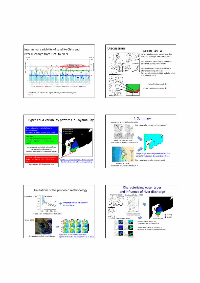
(mgm-3) (m3sec-1)
Chl-a
con
centra5o
n
0
300
600
900
1200
0.1
1
10
100
MJ JASO MJ JASO MJ JASO MJ JASO MJ JASO MJ JASO MJ JASO MJ JASO MJ JASO MJ JASO MJ JASO MJ JASO
1998 1999 2000 2001 2002 2003 2004 2005 2006 2007 2008 2009
RD Subarea-A Subarea-A Subarea-B Subarea-B Subarea-C Subarea-C
Riverd
ischarge
Satellitechl-ainsubareaAishigherislateryearsthanearlieryearsThreis
InterannualvariabilityofsatelliteChl-aandriverdischargefrom1998to2009
Higherthanearlieryears
Tsujimoto Noseasonalvaria5onwasobservedinnutrientsfromApr2006toFeb2008NutrientswasalwayshigherthanthethresholdsatJinzurivermouthNutrientlimita5onwasalteredattheoffshoresta5on(Sta5on3)(Nitrogenlimita5onin2006andphosphatelimita5onin2007)
Discussions
Sta5on3inSub-areaB
Sta5on1and2inSub-areaA
Nutrientsarerichthroughtheyear
UnconsumesnutrientsinsubareaAaretransportedtothissub-area.
Nutrientlimi5ngfactorchangeseachyear.
Twopeakspakerntypicallyfoundintemperatezone(Personetal.1984;Yamadaetal.2004))
Sub-areaASub-areaBSub-areaC
Sub-areaASub-areaBSub-areaC
Spa5alandtemporallydensedatawereusedTocharacterizewatertypesinToyamaBay
MiddletypeChl-aincreaseaferspringtowardssummer,butpeakisnotasclearassub-areaA.
Onelongpeakpakernappearsinsummer(NagataandNakura1993;Ohnishietal.2007)
Typeschl-avariabilitypakernsinToyamaBay 4.Summary
KahruandMitchell,2008
Gohinetal.,2008
AssessmentbytrendofsatelliteChl-a
AssessmentbyLevelofsatelliteChl-a
AssessmentbytrendofsatelliteChl-a
Notenoughpreven5vemanagement.
Notenoughformi5ga5oninterven5on
Singleimageindicatespoten5aleutrophiczonesformi5ga5on&preven5veac5ons
Boyceetal.2010
Decadal-scalephytoplanktonfluctua5ons
IOCCG2000
Chl-aes5ma5onfailsinturbidwaterApplica5onofbekerChl-aes5ma5onalgorithmforturbidwater(Siswantoetal.2011)
Limita5onsoftheproposedmethodology
Integra5onwithhistoricalinsitudata
Characterizingwatertypesandinfluenceofriverdischarge
Sub-areaASub-areaBSub-areaC
Tsujimoto(2012) NagataandNakura(1993)
Ohnishietal.(2007) TNfromJinzuRiver
DeepenunderstandingonChl-avariabilityInToyamabay
Clarifiedboundariesofinfluenceofland-basedsourcesnutrientsfromrivers
jimu
タイプライターテキスト
116
5.Introduc5ontoGoogleEarthEngine
hkps://earthengine.google.com/Thisisthefirstmapofforestchangethatisgloballyconsistentandlocallyrelevant.Whatwouldhavetakenasinglecomputer15yearstoperformwascompletedinamakerofdaysusingGoogleEarthEnginecompu5ng.
-ProfessorMa4Hansen,UniversityofMaryland�
Detec5onofGlobalForestChangeat30mresolu5on
Hansenetal.2013
Analysisofsurfacewaterchangesgloballyat30mresolu5on
Landtowater
WatertoLand
Donchytsetal.2015
Landreclama5oninIsahayaBay,Japan
Handson• Analysisof5meseriesChl-ausingWIMSofware
hkp://wimsof.com
#1.Createimageforyourareaofinterest
• References– C:\ProgramFiles\WimSof\Course\3
• Tutorial_5me_series_of_areal_sta5sics.pdf
• Input– Projec5on:Linear– Pixelinsize9,000meters– Inputla5tudeandlongitudeforyourareaofinterest
– Applycoastallineoverlay• Output
– Saveoutputashdffile
jimu
タイプライターテキスト
117
#2.Createmaskimagesforyourareaofinterest
• References– C:\ProgramFiles\WimSof\Course\3
• Tutorial_5me_series_of_areal_sta5sics.pdf
• Input– Drawmaskstobeusedfor5meserieswithEdit-Drawfunc5on
– Replacecoastlinevalue255with0byTransf-ReplaceValues
• Output– Saveoutputashdffile
#3.Create5meserieschart• References
– C:\ProgramFiles\WimSof\Course\3• Tutorial_5me_series_of_areal_sta5sics.pdf
• Input– RemappedmergedL3MonthlyChl_9imageswithWIMlinerprojec5onbywam_series(savethefilesin“cut”directory)
– ListofmonthlyChl-aimageunderC:\Sat\Merged\L3\Monthly\CHL_9
– Yourcreatedmaskimagefor5meseries• Output
– Runwam_sta5sformonthly5meseriesandsaveoutputas.csvfileandthencreate5meserieschartwithMSexcel
SaveyouroutputinZ(sharedrive)
• #1.Crea5ngdirectorywithyourname• #2.SaveyouroutputinMSpowerpointandputinthedirectory
jimu
タイプライターテキスト
118
E2: Cruise Data Analysis Joji Ishizaka (Institute for Space-Earth Environmental Research, Nagoya University) Abstract
Ise Bay is one of heavily used coastal environments in Japan. Surrounded by the large city of Nagoya and Tokai industrial regions, many cargo ships transported large amount of materials through the bay. Because of the anthropogenic activities, both atmosphere and marine environments had been heavily polluted during 1970/80s, and hypoxia condition of the bottom water has been still often observed during summer, even the loading of the pollutant has been reduced. On the other hand, Ise Bay and the surrounded area have been also known as high fisheries production areas, and some of fish/clam catches, such as Manila clam, is top level in Japan.
Using the T/V Seisui-Maru in Mie University, we will observe marine environments of Ise Bay including water mass structure, phytoplankton abundance, and optical properties. We also demonstrate to take plankton samples by net and sediment with grab. Observations will be conducted in the western Ise Bay (narrow definition of Ise Bay) and in the eastern Ise Bay (Mikawa Bay). It is possible to see how people are using the bay and surrounded areas.
During the excise of cruise data analysis, we are planning to plot environmental data, such as temperature, salinity, chlorophyll-a, from the cruise during the training course and from cruises during different seasons to check the special and temporal changes of the environments. We are going to use Ocean Data View, which is a free software developed by NOAA. We are also planning to verify the chlorophyll-a concentrations estimated by optical measurements and satellite using the observed data during the cruise.
119

120
E3: Coastal model output analysis Hidenori Aiki (Institute for Space-Earth Environmental Research, Nagoya University) Abstract
Ocean models have been used for understanding the three-dimensional structure and the continuous time evolution of coastal ocean circulations that are affected by the seasonal and interannual variations of general ocean circulations, such as the Kuroshio Current. Recent advances in atmosphere-ocean modeling and in-situ and satellite observations have enabled to take into account both the realistic structure of the Kuroshio Current and the high-resolution variations of atmospheric and tidal forcing for ocean circulations. The first part of this exercise gives a short lecture on basic understanding for (i) ocean models, (ii) classification of model experiments, and (iii) available model outputs and forcing. Then the second part of this exercise illustrates how to use a visualization tool suitable for analyzing model outputs and explain useful metrics for understanding the dynamics of coastal ocean circulation.
121

122
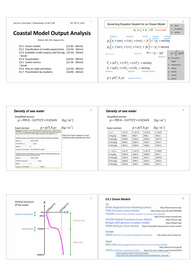
Exercise3,December7(Wednesday),13:30-17:0026thIHPTC,2016
CoastalModelOutputAnalysis�HidenoriAiki,ISEE,NagoyaUniv.�
E3.1Oceanmodels(13:30-20min)E3.2ClassificaOonofmodelexperiments(13:50-20min)E3.3Availablemodeloutputsandforcing(14:10-20min)-break-E3.4VisualizaOon(14:50-30min)E3.5Usefulmetrics(15:10-30min)-break-E3.6HowtomakeanimaOon(15:50-40min)E3.7PresentaOonbystudents(16:40-20min)
��
ux + vy +wz = 0
ρ0 ut + (uu)x + (vu)y + (wu)z − fv⎡⎣ ⎤⎦ = − px +mixing
ρ0 vt + (uv)x + (vv)y + (wv)z + fu⎡⎣ ⎤⎦ = − py +mixing
0 = − pz − gρ
Tt + (uT )x + (vT )y + (wT )z = mixingSt + (uS)x + (vS)y + (wS)z = mixing
ρ = ρ(T ,S, p)
Governing Equation System for an Ocean Model�
equaOonofstate
tendency��������advecOon� Coriolis� pressuregradient�
turbulentviscosity�
turbulentviscosity�
hydrostaOc�
η
TSρfg
seasurface
height
temperature
salinity
density
Coriolis
gravity�
uvw
zonal
meridional
verOcal
tendency�������������advecOon�
Incompressible
p = gρ dzz
η
∫buoyancy�
Boussinesq�
��
Density of sea water�
ρ = ρ(T,S,p) [kg / m3]Exactversion�
Simplifiedversion�ρ ≈ 999.8 − 0.0752T+ 0.8244S [kg / m3]
hZp://co2.hyarc.nagoya-u.ac.jp//labhp/member/aiki/density.html�
�� Density of sea water�
z=0m� T=0 � T=10 � T=20 � T=30 �
S=0g/kg� 999.8� 999.7� 998.2� 995.6�
S=30g/kg� 1024.0� 1023.0� 1020.9� 1017.9�
S=35g/kg� 1028.1� 1026.9� 1024.7� 1021.7�
S=40g/kg� 1032.1� 1030.8� 1028.5� 1025.4�
z=-4000m� T=0 � T=10 � T=20 � T=30 �
S=0g/kg� 1001.8� 1001.6� 1000.0� 997.4�
S=30g/kg� 1025.9� 1024.8� 1022.7� 1019.6�
S=35g/kg� 1030.0� 1028.7� 1026.5� 1023.4�
S=40g/kg� 1034.0� 1032.6� 1030.3� 1027.1�
ρ = ρ(T,S,p) [kg / m3]Exactversion�
Simplifiedversion�ρ ≈ 999.8 − 0.0752T+ 0.8244S [kg / m3]
��
z
l0m-50m
-1000m
-4000m
1025kg/m^3
1027kg/m^3
VerOcalstructureoftheocean�
oceanicmixedlayer�
thermocline�
Surfacelayer�
Deeplayer�
�� E3.1OceanModels�USROMS(RegionalOceanModelingSystem)hZp://www.myroms.org/
POM(PrincetonOceanModel)hZp://www.ccpo.odu.edu/POMWEB/
FVCOM(Finite-Volume,primiOveequaOonCommunityOceanModel)hZp://fvcom.smast.umassd.edu/HYCOM(HybridCoordinateOceanModel)hZps://hycom.org/
MITgcm(MITgeneralcirculaOonmodel)hZp://mitgcm.org/
MOM(ModularOceanModel)hZps://www.gfdl.noaa.gov/mom-ocean-model/EuropeNEMO(NucleusforEuropeanModellingoftheOcean)hZp://www.nemo-ocean.eu/
JapanMRI.COM(MeteorologicalResearchInsOtuteCommunityOceanModel)hZp://www.mri-jma.go.jp/COCO(CCSROceanComponentmodel)hZp://ccsr.aori.u-tokyo.ac.jp/~hasumi/COCO/
OceanmodellingacOviOesintheEastAsiaRegion:hZp://www.clivar.org/sites/default/files/documents/wgomd/tsujino_report.pdf�
�
jimu
タイプライターテキスト
123

VerOcalGridArrangement���Z-levelcoordinatesSigmacoordinatesDensitycoordinates
HorizontalGridArrangement��
E3.1OceanModels�
CEE262c Lecture 8 3
Figure 2: Common vertical coordinate systems used in ocean models.
where ! = !xe1 + !ye2 and V = Ue1 + V e2, and where the horizontal di!usion is given by
Fx =!"xx!x
+!"xy!y
,
"xx = 2AM!U
!x,
"xy = AM
!!U
!y+
!V
!x
"
,
Fx =!
!x
!
2AM!U
!x
"
+!
!y
#
AM
!!U
!y+
!V
!x
"$
.
Note that in the Navier-Stokes equations in their incompressible form, the viscous term isgiven by
!"ij!xj
=!
!xj#
!!ui
!xj+
!uj
!xi
"
= #!2ui
!xj!xj,
so for i = 1, if # "=constant,
!"ij!xj
=!
!x#
!!u
!x+
!u
!x
"
+!
!y#
!!u
!y+
!v
!x
"
+!
!z#
!!u
!z+
!w
!x
"
.
CEE262c Lecture 8 3
Figure 2: Common vertical coordinate systems used in ocean models.
where ! = !xe1 + !ye2 and V = Ue1 + V e2, and where the horizontal di!usion is given by
Fx =!"xx!x
+!"xy!y
,
"xx = 2AM!U
!x,
"xy = AM
!!U
!y+
!V
!x
"
,
Fx =!
!x
!
2AM!U
!x
"
+!
!y
#
AM
!!U
!y+
!V
!x
"$
.
Note that in the Navier-Stokes equations in their incompressible form, the viscous term isgiven by
!"ij!xj
=!
!xj#
!!ui
!xj+
!uj
!xi
"
= #!2ui
!xj!xj,
so for i = 1, if # "=constant,
!"ij!xj
=!
!x#
!!u
!x+
!u
!x
"
+!
!y#
!!u
!y+
!v
!x
"
+!
!z#
!!u
!z+
!w
!x
"
.Oceanography Vol. 19, No. 1, Mar. 200680
A state-of-the-art coastal ocean cir-
culation model system requires: (1) grid
fl exibility to resolve complex coastline
and bathymetry; (2) accurate numerical
methods that conserve mass, momen-
tum, heat, and salt; (3) proper param-
eterization of vertical and horizontal
mixing; (4) modular design to facilitate
selection of the essential model compo-
nents needed in scientifi c or manage-
ment applications; and (5) the ability
to use a wide variety of input data, es-
pecially as more real-time atmospheric
and coastal ocean measurements become
available for assimilation. This model
system should be robust, have a fl exible
user interface, and be an “open” commu-
nity model, supported by an expanding
base of users that continue to improve it.
A major step towards such a system
has been taken recently by a team of
University of Massachusetts-Dartmouth
and Woods Hole Oceanographic Institu-
tion researchers (Chen et al., 2003; Chen
et al., 2004) who have developed a new
prognostic, unstructured-grid, Finite-
Volume, free-surface, three-dimensional
primitive equation Coastal Ocean circu-
lation Model (FVCOM) for physical and
coupled physical/biological studies in
coastal regions characterized by complex
coastlines and bathymetry and diverse
forcing. Used widely in computational
fl uid mechanics and engineering, the
fi nite-volume method used in this model
combines the advantage of fi nite-ele-
ment methods for geometric fl exibility
and fi nite-difference methods for simple
discrete computation (Figure 1). Verifi ed
through comparisons with analytical so-
lutions and numerical simulations made
with POM and other popular fi nite-dif-
ference models in idealized test cases
(Chen et al., submitted), FVCOM has
been successfully applied in a number of
estuarine, continental shelf, and region-
al/open ocean studies involving realistic
model domains (for more information
see http://codfi sh.smast.umassd.edu).
For hindcast and forecast applications,
an integrated coastal ocean model sys-
Changsheng Chen ([email protected]) is Professor, School for Marine Science and Technology, University of Massachusetts-Dartmouth, New Bedford, MA, USA. Robert C. Beardsley is Scientist Emeritus, Depart-ment of Physical Oceanography, Woods Hole Oceanographic Institution, Woods Hole, MA, USA. Geo! rey Cowles is Research Scientist, School for Marine Science and Technology, University of Massachusetts-Dartmouth, New Bedford, MA, USA.
Structured Grid Unstructured Grid
Real Coastline
Ocean
Model Coastline
Figure 1. An example of fi tting a structured grid (left) and an unstructured grid (right) to a simple coastal embayment. ! e true coastline is shown in black, the model coastline in red. Note how the unstructured triangular grid can be adjusted so that the model coastline follows the true coastline, while the structured grid coastline is jagged—which can result in unrealistic fl ow disturbance close to the coast.
� E3.2AvailableModelOutputsandForcing�hZp://apdrc.soest.hawaii.edu�
��
OCEANMODEL
SST
Momentum Heat&Waterflux
AtmosphericForcing
IniOalandlateralboundarycondiOonsforOCEANMODELw/oOdes
�� E3.2AvailableModelOutputsandForcing�hZp://apdrc.soest.hawaii.edu�
���
E3.2AvailableModelOutputsandForcing�
hZp://volkov.oce.orst.edu/Odes/global.html�
���
LombokStrait�Gordon et al. (2005)�
���
jimu
タイプライターテキスト
124
x�
z�
x�
y�
North (Java Sea)�
South (Indian Ocean)�
��� ���
Forcingcheckpoints�
Atmosphericforcingsource:Satelliteremotesensing(dx=20km)orAtmosphericmodeloutputs(global:dx=200km,regional:dx=5km)Ome-evoluOon:Climatology,Monthly,Daily-mean,3-hourinterval,HourlyRiverdischargeincludedornotincludedTidalforcingincludedornotincludedconsOtuents:M2,S2,M1,O1…
��� E3.3Classifica?onofmodelexperiments�
OceanModel• Hindcastexperimentsw/oOdes• Reanalysis(dataassimilaOon)w/oOdes• Nowcastexperimentsw/oOdes• Forecastexperimentsw/oOdes
CoupledAtmosphere-OceanModel• Hindcastexperiments• Reanalysis(dataassimilaOon)• Nowcastexperiments• Forecastexperiments
��
JCOPE (Japan Coastal Ocean Predictability Experiment)�
reanalysis / forecast system
Reanalysis(1993-,dx=1/12deg,108-180E,10.5-62N)
Earth Simulator III�
Earth Simulator III�
�� JCOPE (Japan Coastal Ocean Predictability Experiment)�
reanalysis / forecast system Miyazawa and Yamagata (2003)
Miyazwa et al. (2009) Varlamov et al. (2015)�
���
jimu
タイプライターテキスト
125
OCEANMODEL
SST
Momentum Heat&Waterflux
Atmosphere Model�
OCEANMODEL
SST
Momentum
Heat&Waterflux
Momentum
AtmosphericForcing
IniOalandlateralboundarycondiOonsforOCEANMODELw/oOdes
��� CPU8 CPU7 CPU6 CPU5 CPU4 CPU3 CPU2 CPU1
CloudResolvingStormSimulator(CReSS)
NagoyaUniv.(TsubokiandSakakibara,2003)DX=4km
IniOalandlateralB.C.:RANALfromNPD/JMA
JAMSTEC(AikiandYamgata,2004)DX=4km,DZ=2mfortop100m
IniOalandlateralB.C.:JCOPE2reanalysis:realisOc3DstructureofKuroshioCurrent/SSTinwesternNorthPacific
NonHydrostaOcOceanmodelfortheEarthSimulator(NHOES)
���
��� ���
CPU8 CPU7 CPU6 CPU5 CPU4 CPU3 CPU2 CPU1
CloudResolvingStormSimulator(CReSS)
JAMSTEC(AikiandYamgata,2004)DX=4km,DZ=2mfortop100m
IniOalandlateralB.C.:JCOPE2reanalysis:realisOc3DstructureofKuroshioCurrent/SSTinwesternNorthPacific
NagoyaUniv.(TsubokiandSakakibara,2003)DX=4km
IniOalandlateralB.C.:RANALfromNPD/JMA
NonHydrostaOcOceanmodelfortheEarthSimulator(NHOES)
SurfaceWaveModelMiamiUniv./USA(Donelanetetal,2012)VectorelizedforES
DX=4km�
���
OCEANMODEL
SST
Momentum Heat&Waterflux
Atmosphere Model�
OCEANMODEL
SST
Momentum
Heat&WaterfluxSURFACEWAVEMODEL
Momentum
AtmosphericForcing
IniOalandlateralboundarycondiOonsforOCEANMODELw/oOdes
���
jimu
タイプライターテキスト
126
Sullivan & McWilliams (2010) ���
SurfaceWaveModel�
E x, y,!,"( )σ
Eθ
Wave energy�
Wave direction [rad] 24 grid�
Wave frequency [1/s] 36 grid�
Spectral distribution of wave energy at a fixed point southwest of a hurricane translating north-westward (green arrow) Wave direction (contour) is not the same as wind direction (red arrow) �
distributed in 4-dimensional space: high computational cost
Donelan et al. 2012 / Miami Univ.�
��
Morimotoetal.(2009)
10-m
dep
th
Observed Current Speed�
Before typhoon�
After typhoon�
Observed Temperature�
��
Color: Significant Wave Height (m) Contour: Wind Speed
Color: SST Contour: Sea Surface Pressure
Simulation with wave� T0505 Haitang (2005.07.14-)�
���
E3.4Visualiza?on�Open-sourceSooware
GrADS(GridAnalysisandDisplaySystem)Supportedfileformats:binary(streamorsequenOal),GRIB,NetCDFetc.Supportedremote-accessprotocol:OPeNDAP
hZp://cola.gmu.edu/grads/
Minimumstartdatafile+controlfiletypeeachcommandMediumstartdatafile+controlfileexeccommand-setfile(noloop)Experiencedstartdatafile+controlfilerunprogramfile(withloop)Smartstartremoteaccesstodatawithoutcontrolfile
���
Color: SST Contour: Sea Surface Pressure
Simulation with wave�
Color: Significant Wave Height (m) Contour: Wind Speed
T1013 Megi (2010.10.14-)�
���
jimu
タイプライターテキスト
127
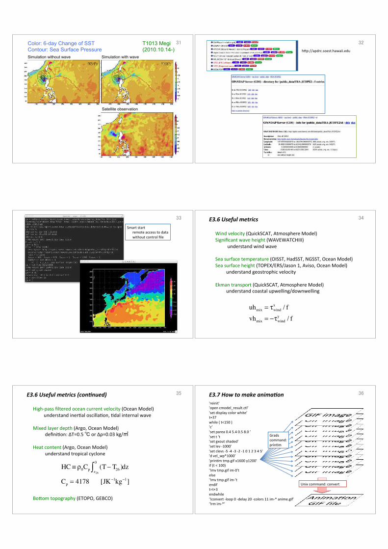
Color: 6-day Change of SST Contour: Sea Surface Pressure Simulation without wave� Simulation with wave�
Satellite observation�
T1013 Megi (2010.10.14-)�
���
hZp://apdrc.soest.hawaii.edu�
���
Smartstartremoteaccesstodatawithoutcontrolfile
��� Windvelocity(QuickSCAT,AtmosphereModel)Significantwaveheight(WAVEWATCHIII)understandwindwaveSeasurfacetemperature(OISST,HadSST,NGSST,OceanModel)Seasurfaceheight(TOPEX/ERS/Jason1,Aviso,OceanModel)understandgeostrophicvelocityEkmantransport(QuickSCAT,AtmosphereModel)understandcoastalupwelling/downwelling
uhmix = τwindx / f
vhmix = −τwindy / f
E3.6Usefulmetrics� ���
High-passfilteredoceancurrentvelocity(OceanModel)understandinerOaloscillaOon,Odalinternalwave�Mixedlayerdepth(Argo,OceanModel)definiOon:ΔT=0.5 orΔρ=0.03kg/�Heatcontent(Argo,OceanModel)understandtropicalcycloneBoZomtopography(ETOPO,GEBCO)
HC ≡ ρ0Cp (T− T26 )z26
0
∫ dz
Cp = 4178 [JK−1kg−1]
E3.6Usefulmetrics(con?nued)� ��� E3.7Howtomakeanima?on�'reinit''opencmodel_result.ctl’'setdisplaycolorwhite’t=37while(t<150)'c’'setparea0.45.40.58.0’'sett't'setgxoutshaded''setlev-1000''setclevs-5-4-3-2-1012345''dvel_wp*1000’'prinOmtmp.gifx1600y1200’if(t<100)'!mvtmp.gifim-0'telse'!mvtmp.gifim-'tendift=t+3endwhile'!convert-loop0-delay20-colors11im-*anime.gif''!rmim-*’
Unixcommand:convert�
Gradscommand:prinOm�
��
jimu
タイプライターテキスト
128
Related Documents