23618-85406-1-PB

Earth Science Research; Vol. 2, No. 2; 2013 ISSN 1927-0542 E-ISSN 1927-0550

Published by Canadian Center of Science and Education

52

Development of a Global Oil Spill Modeling System

William B. Samuels1, David E. Amstutz1, Rakesh Bahadur1 & Christopher Ziemniak1 1 Science Applications International Corporation, Center for Water Science and Engineering, McLean, VA, USA

Correspondence: William B. Samuels, Center for Water Science and Engineering, Science Applications International Corporation, McLean, VA 22102, USA. Tel: 1-703-676-8043. E-mail: [email protected]

Received: January 5, 2013 Accepted: January 23, 2013 Online Published: March 6, 2013

doi:10.5539/esr.v2n2p52 URL: http://dx.doi.org/10.5539/esr.v2n2p52

Abstract

This paper describes the development of an oil spill modeling system that is operational on a global scale and can be used for both real-time response, forecast simulations and probabilistic risk analysis based on climatological wind and ocean current data. For ocean and estuarine spills, the system makes use of the General NOAA Operational Modeling Environment (GNOME) oil spill model, Trajectory Analysis Planner and the Automated Data Inquiry for Oil Spills weathering model. Hydrodynamic and meteorological data is obtained from the US Navy and National Oceanic and Atmospheric Administration. Data access is provided through the Naval Oceanographic Office, the Fleet Numerical Meteorological and Oceanographic Center and the GNOME Online Oceanographic Data Server. For riverine spills, the GeoSpatial Stream Flow Model and the Incident Command Tool for Drinking Water Protection are used to respectively, build river networks with associated flows and velocities and, transport and disperse oil spill contamination downstream. Case study examples are presented for both forecast simulations and probabilistic risk analysis.

Keywords: coastal ocean, estuarine, riverine, transport, dispersion

1. Introduction

The Exxon Valdez (EVOS, 2012) and Deepwater Horizon (NOAA, 2012a) oil spills have highlighted the potential for human caused environmental damage. In attempting to mitigate or avoid future damage to valuable natural resources caused by marine pollution, research has been undertaken by the scientific community to study the processes affecting the fate and distribution of environmental pollution, and especially to model and simulate these processes.

One area of research has been computational Lagrangian transport or trajectory modeling. Trajectory models attempt to predict the movement of actual or hypothetical pollution spills. All existing computerized trajectory models have their advantages and disadvantages. The development of the General NOAA Operational Modeling Environment (GNOME) resulted in a comprehensive model that is easy to set up and which has been validated against observations for many oil spill events (NOAA, 2002; Beegle-Krause, 2001). GNOME is used as a forecasting tool for both actual spill events and a planning tool to examine “what-if” scenarios. Data can come from a variety of sources including direct observations and models of winds and currents. For example, the US Naval Oceanographic Office (NAVO, 2012) runs coastal and ocean models for many parts of the world. NAVO generates velocity vectors, temperature, and salinity for currents in support of fleet operations. The NAVO output can also be used as input to ocean contamination models (e.g., the NAVO surface currents as input to the GNOME model (NOAA, 2010).

In addition to trajectory modeling using Lagrangian transport, network-based models have been developed and applied to spills occurring in riverine environments. The Incident Command Tool for Drinking Water Protection (ICWater) (Samuels & Ryan, 2005) uses the National Hydrography Dataset Plus (NHDPlus) for downstream transport and dispersion of oil spills in US rivers (NHDPlus, 2012). For areas outside the US (where NHDPlus does not exist), river networks are built with the GeoSpatial Stream Flow Model (GeoSFM) (Asante et al., 2008). These networks, in turn, are incorporated into ICWater for spill transport and dispersion.

The ability to rapidly predict oil spill trajectories in real-time on a global scale has been achieved through the integration of oil spill modeling tools with forecast hydrodynamic and meteorological datasets available on the internet. Easy access to historical data has also enabled the ability to perform probabilistic spill analysis in a

www.ccsenet.org/esr Earth Science Research Vol. 2, No. 2; 2013

53

timely manner. This paper describes these tools and datasets and their successful integration into a global oil spill modeling system.

2. Oil Spill Modeling Tools

2.1 Ocean and Estuarine Domain

The oil spill modeling tools used for ocean and estuarine modeling are public domain software available from the National Oceanic and Atmospheric Agency (NOAA). These tools include the GNOME oil spill model, Trajectory Analysis Planner (TAP), and the Automated Data Inquiry for Oil Spills (ADIOS). Each of these individual tools is described in more detail below. For this system, both real-time and probabilistic modeling capabilities were set up for oil spill scenarios. For the probabilistic analysis, a series of python scripts were developed to perform a Monte Carlo simulation of the GNOME oil spill model. Output was passed to the TAP software to calculate spill probabilities on a regular grid. This data was converted to GIS shapefile and KML formats for inclusion in standard reports.

2.1.1 GNOME

According to Beegle-Krause (2001), “GNOME was designed for the rapid modeling of pollutant trajectories in the marine environment. The overall design is that of modular and integrated software. Maps, coastal outlines and shoreline descriptors, bathymetry, numerical circulation models, statistical climatological simulations, location and type of the spilled substance, oceanographic and meteorological observations, and other environmental data are inputs to GNOME. The output from the model consists of graphics, movies, and data files for post-processing in a GIS system. The GNOME Analyst Tool can be used to calculate spill contours or the Trajectory Analysis Planner (TAP) can be used to calculate oil spill contact probabilities. GNOME is quite general and applies to most trajectory problems. It is a Lagrangian model that is two-dimensional in space, but vertically isolated layered systems can be modeled. Shoreline maps are inputs to the model so any area can be addressed. The model automatically handles either hemisphere and east or west longitude. Shorelines can optionally be coded for environmental sensitivity and displayed on the map.”

2.1.2 TAP

GNOME can be run in batch mode to produce a large number of trajectories under variable environmental conditions. The output from these batch runs is passed to the TAP (NOAA, 2000) software, which is designed to investigate the probabilities that spilled oil will move and spread in particular ways within a specific area. By graphically presenting the results of thousands of oil-spill trajectory simulations, TAP helps emergency planners understand and anticipate many possible outcomes when developing local-area contingency plans for oil spill response. TAP assists with the following planning tasks: (1) assessing potential threats from possible spill sites to a given sensitive location, (2) determining which shoreline areas are most likely to be threatened by a spill originating from a given location, (3) calculating the probability that a certain amount of oil will reach a given site within a given time-period and (4) estimating the levels of impact on a given resource from a spill.

2.1.3 ADIOS

ADIOS is NOAA's oil weathering model. ADIOS integrates a library of approximately one thousand oils with a short-term oil fate and cleanup model to help estimate the amount of time that spilled oil will remain in the marine environment, and to develop cleanup strategies (NOAA, 2012b). ADIOS calculations combine real-time environmental data, such as wind speed, with chemical and physical property information in its oil library. The program provides output on oil weathering parameters such as evaporation, dispersion into the water column, and changes in oil density and viscosity.

2.2 Riverine Domain

The oil spill modeling tools for the riverine environment included public domain tools from the Defense Threat Reduction Agency and the US Geological Survey. These tools include ICWater and GeoSFM. Each of these tools is described in more detail below. Spill modeling in rivers is based on a hydrologically connected river network with associated mean flows and velocities. These flows and velocities can be updated using output from real-time stream flow gages to adjust the mean flows up or down. Assets such as drinking water intakes are indexed to the river network to enable consequence assessment to downstream populations and critical infrastructure.

2.2.1 ICWater

According to the ICWater fact sheet (Horizon Systems, 2012), “ICWater is structured around the RiverSpill (Samuels et al, 2006) model which has been enhanced to make use of the 1:100,000 scale NHDPlus for


54

applications in the US. ICWater is GIS-based tool and includes the NHDPlus, a hydrologically connected river network that contains over 3 million reach segments in the US. This allows for both downstream and upstream network navigation. Mean flow and velocity has been calculated by the USGS and EPA for each reach. RiverSpill provides real-time assessments of the travel and dispersion of contaminants in streams and rivers. Stream and river flows used in ICWater are derived from web accessible real-time gauging stations maintained throughout the country by the USGS. Example databases available within ICWater include: dams, reservoirs, public drinking water intakes, stream gages, municipal and industrial dischargers and transportation networks.” For applications outside of the US, ICWater uses river networks developed by GeoSFM.

2.2.2 GeoSFM

The USGS Earth Resources Observation and Science Data Center has implemented a hydrologic modeling system which consists of an operational data processing system and a geospatial stream flow model (Asante et al., 2008). GeoSFM’s data processing system generates evapotranspiration (USGS, 2007) and precipitation (Joyce et al., 2007) data from a variety of remotely sensed sources on a daily basis. To allow for rapid implementation in data scarce environments, widely available terrain (SRTM, 2012) soil (FAO, 1997) and land cover (USGS, 2006) datasets are used for model setup and initial parameter estimation. GeoSFM performs geospatial pre-processing and post- processing tasks as well as hydrologic modeling tasks within a Geographic Information System (GIS) environment.

3. Data

3.1 Ocean and Estuarine Environment

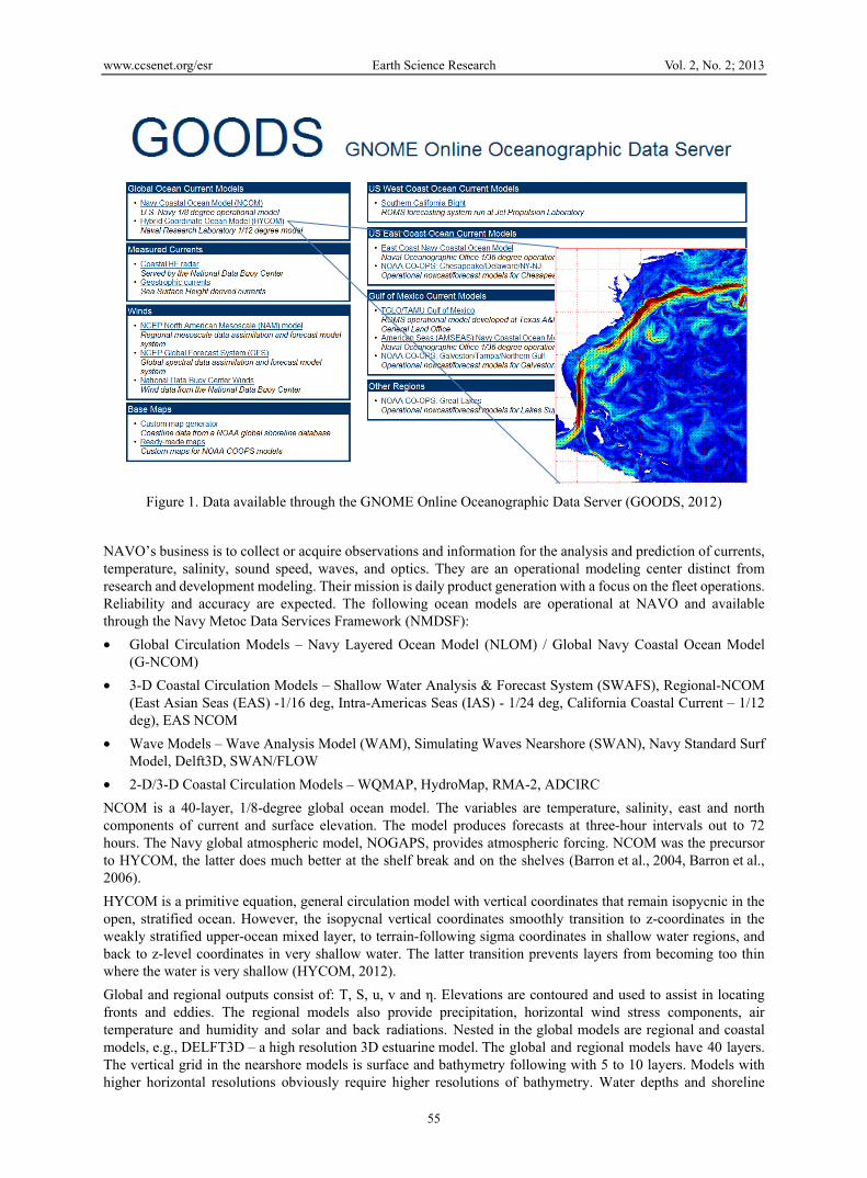
The data required for oil spill modeling includes ocean currents, winds, tides, coastline boundary and a database of oil properties (required as input for oil weathering algorithms). For forecast winds and currents, NOAA has built the GNOME Online Oceanographic Data Server (GOODS, 2012) that provides access to a large majority of the datasets required to run the GNOME oil spill model (see Figure 1). In addition, NAVO provides real-time output from global ocean forecast models including the Navy Coastal Ocean Model (NCOM) (Barron et al., 2004, Barron et al., 2006) and the Hybrid Coordinate Ocean Model (HYCOM, 2012). Wind forecast data was obtained from the National Centers for Environmental Prediction (NCEP) Global Forecast System (GFS, 2012). Digital representations of the coastline are available through NOAA’s Global Self-consistent, Hierarchical, High-Resolution Shoreline Database (GSHHS, 2012). Climatological ocean current datasets were obtained from the US Navy Fleet Numerical Meteorological and Oceanographic Center (FNMOC) through the Global Ocean Data Assimilation Experiment (GODAE, 2012). Climatological wind data was provided by global reanalysis dataset created jointly by NCEP and the National Center for Atmospheric Research (NCAR) (Kalnay et al., 1996; Kistler et al., 2001).

3.1.1 GOODS

GOODS is an online tool that helps GNOME users access base maps and publicly available ocean currents and winds from various models and data sources. Users can then download the files in a format that can be read directly into GNOME (e.g., map files in BNA format; current and wind files in netCDF). Datasets can be subset by geographic coordinates (latitude/longitude bounding box) and time (beginning date, forecast duration and time step).

3.1.2 Ocean Currents

NAVO, based at the John C. Stennis Space Center in Mississippi, continually collects oceanographic data around the globe. NAVO uses that data to produce a wide variety of oceanographic products and services for the United States Department of Defense along with other US government and international customers including civilian organizations.


55

Figure 1. Data available through the GNOME Online Oceanographic Data Server (GOODS, 2012)

NAVO’s business is to collect or acquire observations and information for the analysis and prediction of currents, temperature, salinity, sound speed, waves, and optics. They are an operational modeling center distinct from research and development modeling. Their mission is daily product generation with a focus on the fleet operations. Reliability and accuracy are expected. The following ocean models are operational at NAVO and available through the Navy Metoc Data Services Framework (NMDSF):

Global Circulation Models – Navy Layered Ocean Model (NLOM) / Global Navy Coastal Ocean Model (G-NCOM)

3-D Coastal Circulation Models – Shallow Water Analysis & Forecast System (SWAFS), Regional-NCOM (East Asian Seas (EAS) -1/16 deg, Intra-Americas Seas (IAS) - 1/24 deg, California Coastal Current – 1/12 deg), EAS NCOM

Wave Models – Wave Analysis Model (WAM), Simulating Waves Nearshore (SWAN), Navy Standard Surf Model, Delft3D, SWAN/FLOW

2-D/3-D Coastal Circulation Models – WQMAP, HydroMap, RMA-2, ADCIRC

NCOM is a 40-layer, 1/8-degree global ocean model. The variables are temperature, salinity, east and north components of current and surface elevation. The model produces forecasts at three-hour intervals out to 72 hours. The Navy global atmospheric model, NOGAPS, provides atmospheric forcing. NCOM was the precursor to HYCOM, the latter does much better at the shelf break and on the shelves (Barron et al., 2004, Barron et al., 2006).

HYCOM is a primitive equation, general circulation model with vertical coordinates that remain isopycnic in the open, stratified ocean. However, the isopycnal vertical coordinates smoothly transition to z-coordinates in the weakly stratified upper-ocean mixed layer, to terrain-following sigma coordinates in shallow water regions, and back to z-level coordinates in very shallow water. The latter transition prevents layers from becoming too thin where the water is very shallow (HYCOM, 2012).

Global and regional outputs consist of: T, S, u, v and η. Elevations are contoured and used to assist in locating fronts and eddies. The regional models also provide precipitation, horizontal wind stress components, air temperature and humidity and solar and back radiations. Nested in the global models are regional and coastal models, e.g., DELFT3D – a high resolution 3D estuarine model. The global and regional models have 40 layers. The vertical grid in the nearshore models is surface and bathymetry following with 5 to 10 layers. Models with higher horizontal resolutions obviously require higher resolutions of bathymetry. Water depths and shoreline


56

locations are problems in many areas, and they can be variable due to storm events. The higher resolution models are essential for treating tidal processes in nearshore areas and extending upwards in rivers to head-of-tide (NAVO, 2012).

3.1.3 Winds

Real-time and forecast winds are obtained through NOAA’s Global Forecast System (GFS, 2012) available through GOODS. GFS is a global spectral data assimilation and forecast model system. Forecasts are produced every six hours at approximately 50-km or 0.5-deg resolution. The vertical domain from the earth's surface (sigma=1) to the top of the atmosphere (sigma=0) is divided into 64 layers with enhanced resolution near the bottom and the top. Atmospheric dynamics are represented by primitive equations with vorticity, divergence, logarithm of surface pressure, specific humidity virtual temperature, and cloud condensate as dependent variables.

3.1.4 Climatology

Climatological ocean current data was obtained through the Global Ocean Data Assimilation Experiment (GODAE, 2012) website. The GODAE vision is to provide: “A global system of observations, communications, modeling and assimilation that will deliver regular, comprehensive information on the state of the oceans, in a way that will promote and engender wide utility and availability of this resource for maximum benefit to the community”. For the global oil spill modeling system we accessed the FNMOC High Resolution Ocean Analysis from GODAE for historical data through June 2006. These data include daily 3D temperature, salinity, geopotential and u,v current fields on a nearly global Mercator grid (2161 longitudes, 1051 latitudes and 34 levels in each file).

Climatological wind data was provided through the Operational Multiscale Environmental model with Grid Adaptivity (OMEGA) (Bacon et al., 2000; Bacon et al, 2003). To generate the high resolution climatology, OMEGA starts with the approximately 2⁰ × 2⁰ resolution (in latitude and longitude) global reanalysis dataset created jointly by the National Centers of Environmental Prediction (NCEP) and the National Center for Atmospheric Research (NCAR) (Kalnay et al., 1996; Kistler et al., 2001). OMEGA refines the NCEP/NCAR dataset by providing high resolution in regions of complex terrain and land/water boundaries.

3.1.5 Coastline

In addition to winds and currents, the oil spill model requires a representation of land and water to establish the model boundary. This system uses the Global Self-consistent, Hierarchical, High-resolution Shoreline (GSSHS, 2012) database accessible through GOODS. GSHHS is a high-resolution shoreline data set amalgamated from two databases in the public domain. The data have undergone extensive processing and are free of internal inconsistencies such as erratic points and crossing segments. The shorelines are constructed entirely from hierarchically arranged closed polygons.

3.2 Riverine Environment

The data required for oil spill modeling in the riverine environment includes a hydrologically connected river network with associated flows and velocities that can be updated by data from real-time stream gauging stations. In the US, the data used is the NHDPlus and USGS real-time stream flow gauging stations. Outside the US, the data used is HydroSHEDS (Hydrological data and maps based on Shuttle Elevation Derivatives at multiple Scales) with associated flows and velocities generated by GeoSFM.

3.2.1 NHDPlus

The NHDPlus contains more than 3 million stream and river reaches, all hydrologically connected. Dams are included as one of the asset databases and can act as barriers in the network. Long-term average values of velocity and flow (discharge) are attributes of the NHDPlus reported for each reach. The real-time gages report stream and river flow from approximately 7,000 sites located throughout the U.S. ICWater uses the relationship between river velocity and river flow to determine the real-time velocity from the measured (gauged) real-time flow. The calculations use the ratio of real-time velocity to long-term average velocity for extrapolation to river reaches not represented by the real-time gage network.

3.2.2 HydroSheds

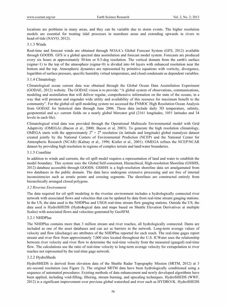
HydroSHEDS is derived from elevation data of the Shuttle Radar Topography Mission (SRTM, 2012) at 3 arc-second resolution (see Figure 2). The original SRTM data have been hydrologically conditioned using a sequence of automated procedures. Existing methods of data enhancement and newly developed algorithms have been applied, including void-filling, filtering, stream burning, and upscaling techniques. HydroSHEDS (WWF, 2012) is a significant improvement over previous global watershed and river such as HYDRO1K. HydroSHEDS


57

vector and raster datasets include: stream networks, watershed boundaries, drainage directions, and ancillary data layers such as flow accumulations, distances, and river topology information.

Figure 2. HydroSHEDS data availability – global tiling scheme (USGS, 2012)

4. System Integration and Example Results

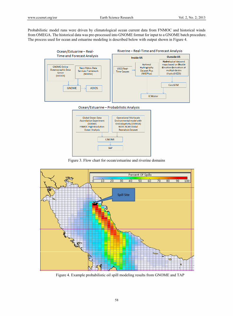
Figure 3 presents a flowchart showing the connection between the modeling tools and data used to operate the global system. For the oceanic environment, we established a linkage to the modeling output generated by NAVO. We download the ocean current and vector files from GOODS and/or the NMDSF. Surface wind data is provided through a number of sources including observations at meteorological stations, output from the NCEP Global Forecast System and the OMEGA weather analysis/forecast system. We run the GNOME model, TAP and ADIOS. GNOME provides the oil spill trajectories, TAP provides the probabilistic analysis of oil spill risk and ADIOS simulates oil weathering processes.

For the ocean/estuarine real-time analysis, a web-based system was developed that accessed forecast ocean currents over the internet. The daily runs take daily forecast winds and currents from the NOAA GOODS website. The sites that are run are entered through the website, run on a daily schedule once the required weather data is available. The running of GNOME is achieved by a windows desktop service which creates a GNOME batch file to run and produce a standardized output for each site. A single release definition is used at all sites as a baseline, for displaying the trend for the modeled period. The release definition is a continuous release of a fixed rate over the entire 72 hour forecast period. After the service has run the model for the set of releases, animations are created using tools to read the output, displaying the tracer elements as well as expected concentrations as a function of time for the duration of the calculation. The website then presents the users with the opportunity to select individual sites, either for the current day, or for previous days to see the expected direction of travel if there were to be a release in the area of the site.

The system described above can also be configured to utilize winds and currents at higher resolutions from other sources, including the NMDSF. NMDSF is a collection of web services which use the Joint METOC Broker Language (JMBL) specifications. It contains default implementations for distributing Network Common Data Form (NetCDF), Gridded Binary (GRIB), and Relational Database Management System (RDBMS) data. The primary component in NMDSF is the Data-Oriented Services (DOS) Framework. The framework is a toolkit for deploying data-oriented services that securely deliver geospatial information consistent with the JMBL specification (NAVO, 2008).


58

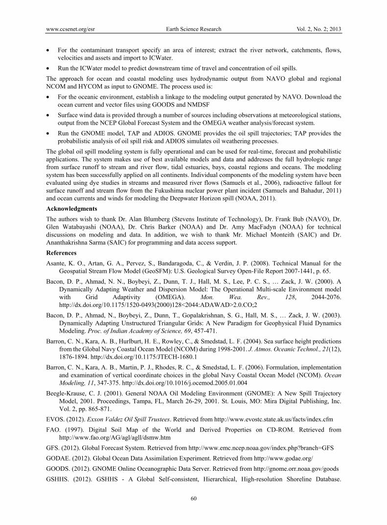
Probabilistic model runs were driven by climatological ocean current data from FNMOC and historical winds from OMEGA. The historical data was pre-processed into GNOME format for input to a GNOME batch procedure. The process used for ocean and estuarine modeling is described below with output shown in Figure 4.

Figure 3. Flow chart for ocean/estuarine and riverine domains

Figure 4. Example probabilistic oil spill modeling results from GNOME and TAP

Spill Site


59

The approach for riverine modeling uses a hydrologically connected river network (NHDPlus in the US, HydroSHEDS outside of the US) for downstream transport and dispersion of oil in non-tidal rivers. For NHDPlus, mean flows and velocities are adjusted based on real-time stream gauge data. A flow factor is calculated based on the ratio of the real-time flow to the mean flow on the reach where the gauge is located. This factor is applied to all the downstream reaches to scale the mean flows and resulting velocities. For HydroSHEDS, mean flows and velocities are generated by GeoSFM using satellite-derived rainfall estimates, evapotranspiration, land use and soils data to calculate water balance and perform discharge routing. The resulting mean flows and velocities can also be adjusted if real-time stream gauge data is available. Example output for a riverine oil spill is shown in Figure 5. This case also shows the drinking water intakes that may be affected.

5. Summary and Conclusions

In this study the project team established collaborations with NOAA and the NAVO data center for implementation of an oil spill model and supporting hydrodynamic data. Specifically, the team implemented a spill modeling tool set consisting of GNOME, ADIOS, GOODS and TAP. The project team also developed data access and processing tools for global and regional hydrodynamic data from the US Navy. Both probabilistic and real-time modeling capabilities were set up for oil spill scenarios. In addition, a watershed and riverine modeling tool set consisting of GeoSFM and ICWater was implemented. ICWater accesses the NHDPlus for oil spill modeling in US rivers. For areas outside the US, GeoSFM in conjunction with HydroSHEDS is used to generate river networks (with associated flows and velocities) for input to ICWater.

Figure 5. Example ICWater oil spill model result in a riverine environment

Oil spill modeling was partitioned into two components: (1) a modeling approach for surface water (i.e., watersheds and rivers) and (2) a modeling approach for ocean and coastal regions. A different suite of modeling tools has been implemented for each modeling domain.

The approach for watersheds and rivers uses GeoSFM to generate river networks, catchments, flows and velocities for input to ICWater. The process followed is:

Prepare the input data for GeoSFM from a set of global databases (terrain, land use, soils, rainfall, and evapotranspiration).

Organize and integrate the input databases so that the specification of an area of interest triggers the extraction of data to run the model.

Automate Hydrology Data Extraction based on Polygon of Interest.

Run GeoSFM

Calibrate and validate the flow/velocities with observed data in the Global Runoff Data Center database or any other set of available observations.

Spill Site

Intake

Spill Trace

Real-Time Gauge


60

For the contaminant transport specify an area of interest; extract the river network, catchments, flows, velocities and assets and import to ICWater.

Run the ICWater model to predict downstream time of travel and concentration of oil spills.

The approach for ocean and coastal modeling uses hydrodynamic output from NAVO global and regional NCOM and HYCOM as input to GNOME. The process used is:

For the oceanic environment, establish a linkage to the modeling output generated by NAVO. Download the ocean current and vector files using GOODS and NMDSF

Surface wind data is provided through a number of sources including observations at meteorological stations, output from the NCEP Global Forecast System and the OMEGA weather analysis/forecast system.

Run the GNOME model, TAP and ADIOS. GNOME provides the oil spill trajectories; TAP provides the probabilistic analysis of oil spill risk and ADIOS simulates oil weathering processes.

The global oil spill modeling system is fully operational and can be used for real-time, forecast and probabilistic applications. The system makes use of best available models and data and addresses the full hydrologic range from surface runoff to stream and river flow, tidal estuaries, bays, coastal regions and oceans. The modeling system has been successfully applied on all continents. Individual components of the modeling system have been evaluated using dye studies in streams and measured river flows (Samuels et al., 2006), radioactive fallout for surface runoff and stream flow from the Fukushima nuclear power plant incident (Samuels and Bahadur, 2011) and ocean currents and winds for modeling the Deepwater Horizon spill (NOAA, 2011).

Acknowledgments

The authors wish to thank Dr. Alan Blumberg (Stevens Institute of Technology), Dr. Frank Bub (NAVO), Dr. Glen Watabayashi (NOAA), Dr. Chris Barker (NOAA) and Dr. Amy MacFadyn (NOAA) for technical discussions on modeling and data. In addition, we wish to thank Mr. Michael Monteith (SAIC) and Dr. Ananthakrishna Sarma (SAIC) for programming and data access support.

References

Asante, K. O., Artan, G. A., Pervez, S., Bandaragoda, C., & Verdin, J. P. (2008). Technical Manual for the Geospatial Stream Flow Model (GeoSFM): U.S. Geological Survey Open-File Report 2007-1441, p. 65.

Bacon, D. P., Ahmad, N. N., Boybeyi, Z., Dunn, T. J., Hall, M. S., Lee, P. C. S., … Zack, J. W. (2000). A Dynamically Adapting Weather and Dispersion Model: The Operational Multi-scale Environment model with Grid Adaptivity (OMEGA). Mon. Wea. Rev., 128, 2044-2076. http://dx.doi.org/10.1175/1520-0493(2000)128<2044:ADAWAD>2.0.CO;2

Bacon, D. P., Ahmad, N., Boybeyi, Z., Dunn, T., Gopalakrishnan, S. G., Hall, M. S., … Zack, J. W. (2003). Dynamically Adapting Unstructured Triangular Grids: A New Paradigm for Geophysical Fluid Dynamics Modeling. Proc. of Indian Academy of Science, 69, 457-471.

Barron, C. N., Kara, A. B., Hurlburt, H. E., Rowley, C., & Smedstad, L. F. (2004). Sea surface height predictions from the Global Navy Coastal Ocean Model (NCOM) during 1998-2001. J. Atmos. Oceanic Technol., 21(12), 1876-1894. http://dx.doi.org/10.1175/JTECH-1680.1

Barron, C. N., Kara, A. B., Martin, P. J., Rhodes, R. C., & Smedstad, L. F. (2006). Formulation, implementation and examination of vertical coordinate choices in the global Navy Coastal Ocean Model (NCOM). Ocean Modeling, 11, 347-375. http://dx.doi.org/10.1016/j.ocemod.2005.01.004

Beegle-Krause, C. J. (2001). General NOAA Oil Modeling Environment (GNOME): A New Spill Trajectory Model, 2001. Proceedings, Tampa, FL, March 26-29, 2001. St. Louis, MO: Mira Digital Publishing, Inc. Vol. 2, pp. 865-871.

EVOS. (2012). Exxon Valdez Oil Spill Trustees. Retrieved from http://www.evostc.state.ak.us/facts/index.cfm

FAO. (1997). Digital Soil Map of the World and Derived Properties on CD-ROM. Retrieved from http://www.fao.org/AG/agl/agll/dsmw.htm

GFS. (2012). Global Forecast System. Retrieved from http://www.emc.ncep.noaa.gov/index.php?branch=GFS

GODAE. (2012). Global Ocean Data Assimilation Experiment. Retrieved from http://www.godae.org/

GOODS. (2012). GNOME Online Oceanographic Data Server. Retrieved from http://gnome.orr.noaa.gov/goods

GSHHS. (2012). GSHHS - A Global Self-consistent, Hierarchical, High-resolution Shoreline Database.


61

Retrieved from http://www.ngdc.noaa.gov/mgg/shorelines/gshhs.html

Horizon Systems. (2012). ICWater fact sheet. Retrieved from http://www.horizon-systems.com/NHDPlus/applications.php

HYCOM. (2012). Hybrid Coordinate Ocean Model. Retrieved from http://hycom.org/hycom/overview

Joyce, R. J., Janowiak, J. E., Arkin, P. A., & Xie, P. (2007). CMORPH: A method that produces global precipitation estimates from passive microwave and infrared data at high spatial and temporal resolution. J. Hydromet., 5, 487-503. http://dx.doi.org/10.1175/1525-7541(2004)005<0487:CAMTPG>2.0.CO;2

Kalnay, E., Kanamitsu, M., Kistler, R., Collins, W., Deaven, D., Gandin, L., … Dennis, J. (1996). The NCEP/NCAR 40-Year Reanalysis Project. Bull. Amer. Met. Soc., 77, 437-471. http://dx.doi.org/10.1175/1520-0477(1996)077<0437:TNYRP>2.0.CO;2

Kistler, R., Kalnay, E., Collins, W., Saha, S., White, G., Woollen, J., …Fiorino, M. (2001). The NCEP-NCAR 50–Year Reanalysis: Monthly Means CD–ROM and Documentation. Bull. Am. Met. Soc., 82, 247-268. http://dx.doi.org/10.1175/1520-0477(2001)082<0247:TNNYRM>2.3.CO;2

NAVO. (2008). User Guide, Navy Metoc Data Services Framework. Retrieved from https://wiki.ucar.edu/download/attachments/17761275/NAVO_JMBL_Users_Guide_DS-UG-20081017.doc

NAVO. (2012). Naval Oceanographic Office. Retrieved from http://www.usno.navy.mil/NAVO

NHDPlus. (2012). National Hydrography Dataset Plus. Retrieved from http://www.horizon-systems.com/nhdplus

NOAA. (2000). Trajectory Analysis Planner II (TAP II) User Manual, Office of Response and Restoration, Hazardous Materials Response Division, May, 2000.

NOAA. (2002). General NOAA Oil Modeling Environment (GNOME) Users Manual, Office of Response and Restoration, Hazardous Materials Response Division, January 2002.

NOAA. (2010). GNOME Data Formats. Office of Response and Restoration, Hazardous Materials Response Division, November, 2010.

NOAA. (2011). DWH – Response Modeling Activities. Retrieved from http://vislab-ccom.unh.edu/~schwehr/2011AkMarSciSym/AkMarSciPaytonModeling.pdf

NOAA. (2012a). NOAA Deepwater Horizon Archive. Retrieved from http://response.restoration.noaa.gov/Deepwaterhorizon

NOAA. (2012b). Automated Data Inquiry for Oil Spills. Retrieved from http://response.restoration.noaa.gov/oil-and-chemical-spills/oil-spills/response-tools/adios.html

Samuels, W. B., & Amstutz, D. E. (2009). Using HydroSHEDS and GeoSFM to Calculate River Discharge, Proceedings, International Perspective on Environmental and Water Resources, January 5-7, 2009, Bangkok, Thailand.

Samuels, W. B., & Bahadur, R. (2011). Surface water transport of radioactivity from the Fukushima Nuclear Power Plant Incident, 10th Symposium on the Coastal Environment, American Meteorological Society Conference, New Orleans, LA, January 22-25, 2012.

Samuels, W. B., & Ryan, D. (2005). ICWater: Incident Command Tool for Protecting Drinking Water, Proceedings ESRI International User Conference, July 25-29, 2005, San Diego, CA.

Samuels, W. B., Amstutz, D. A., Bahadur, R., & Pickus, J. M. (2006). RiverSpill: A National Application for Drinking Water Protection. J. Hydraulic Eng., 132(4), 393-403. http://dx.doi.org/10.1061/(ASCE)0733-9429(2006)132:4(393)

SRTM. (2012). Shuttle Radar Topography Mission. Retrieved from http://srtm.usgs.gov/index.php

USGS. (2006). Global Land Cover Characterization (GLCC). Retrieved from http://eros.usgs.gov/products/landcover/glcc.html

USGS. (2007). Global Potential Evapotranspiration (PET). Retrieved from http://igskmncnwb015.cr.usgs.gov/Global/product.php?image=pt

USGS. (2012). Hydrologically Data and Maps Based on Shuttle Elevation Derivatives at Multiple Scales. http://hydrosheds.cr.usgs.gov/

WWF. (2007). HydroSHEDS Overview. Retrieved from http://www.worldwildlife.org/hydrosheds

23618-85406-1-PB

Documents

oil spill events noaa

oil spill contamination

water science

trajectory modeling

oil spills weathering

oceanographic center

meteorological data

ocean models