PEBS DELIVERABLE (D-N°: 2.2-3) Report of the construction of the HE-E experiment Author(s): Sven-Peter Teodori and Irina Gaus (Ed.) Sven Köhler, Juan Carlos Mayor, Christophe Nussbaum , Ursula Rösli, Kristof Schuster, José-Luis Garcià Siñeriz, Patrick Steiner, Thomas Trick, Hanspeter Weber, Klaus Wieczorek. Reporting period: 01/03/10 – 28/02/11 Date of issue of this report: 15/01/12 Start date of project: 01/03/10 Duration: 48 Months Project co-funded by the European Commission under the Seventh Euratom Framework Programme for Nuclear Research &Training Activities (2007-2011) Dissemination Level PU Public RE Restricted to a group specified by the partners of the [acronym] project CO Confidential, only for partners of the [acronym] project PEBS (Contract Number: FP7 249681)

Welcome message from author
This document is posted to help you gain knowledge. Please leave a comment to let me know what you think about it! Share it to your friends and learn new things together.
Transcript
PEBS
DELIVERABLE (D-N°: 2.2-3)
Report of the construction of the HE-E experiment
Author(s): Sven-Peter Teodori and Irina Gaus (Ed.)
Sven Köhler, Juan Carlos Mayor, Christophe Nussbaum , Ursula Rösli, Kristof Schuster, José-Luis
Garcià Siñeriz, Patrick Steiner, Thomas Trick, Hanspeter Weber, Klaus Wieczorek.
Reporting period: 01/03/10 – 28/02/11
Date of issue of this report: 15/01/12
Start date of project: 01/03/10 Duration: 48 Months
Project co-funded by the European Commission under the Seventh Euratom Framework Programme for Nuclear Research &Training Activities (2007-2011)
Dissemination Level PU Public RE Restricted to a group specified by the partners of the [acronym] project CO Confidential, only for partners of the [acronym] project
PEBS (Contract Number: FP7 249681)


I NAGRA NAB 11-25
Table of Contents
Table of Contents ........................................................................................................................... I
List of Tables.................................................................................................................................V
List of Figures ............................................................................................................................. VI
1 Introduction and objectives ................................................................................... 1
1.1 Context of the experiment ........................................................................................ 1
1.2 Objectives of the experiment .................................................................................... 1
1.3 Reporting related to the experiment ......................................................................... 2
2 Location and general layout of the experiment.................................................... 3
2.1 Characteristics of VE test section ............................................................................. 3
2.1.1 Location and geometry ............................................................................................. 3
2.1.2 Geology of the HE-E test section ............................................................................. 3
2.2 General layout of the experiment ............................................................................. 5
2.3 Description of the initial conditions of the site......................................................... 7
2.4 Site preparation and infrastructure activities .......................................................... 10
2.4.1 Definition of the reference system for the HE-E experiment ................................. 12
2.4.2 Location of the HE-E experiment inside RB micro tunnel..................................... 14
2.4.3 Railway emplacement............................................................................................. 14
2.4.3.1 Railway leveling and concreting ............................................................................ 15
2.4.4 Temporary steel nets............................................................................................... 18
2.5 Time schedule......................................................................................................... 19
3 Materials and methods ......................................................................................... 21
3.1 Bentonite blocks ..................................................................................................... 21
3.1.1 Design and fabrication............................................................................................ 21
3.1.2 Handling and transportation ................................................................................... 22
3.1.3 Laboratory tests ...................................................................................................... 23
3.2 Sand/bentonite mixture........................................................................................... 24
3.2.1 Fabrication and properties ...................................................................................... 24
3.2.2 Handling and transportation ................................................................................... 24
3.3 Granular bentonite material .................................................................................... 24
3.4 Emplacement of buffer material ............................................................................. 25
3.4.1 Requirements .......................................................................................................... 25
3.4.2 Chosen emplacement technique ............................................................................. 25
3.4.3 Machinery description and pre-test procedures ...................................................... 26
3.4.3.1 Description of the machinery construction............................................................. 26
3.4.3.2 Full-scale pre-test in concrete and wood tubes....................................................... 26
3.4.3.3 Optimization of the bentonite emplacement procedure .......................................... 28
3.4.3.4 Effect of compaction by a concrete vibrator........................................................... 30

NAGRA NAB 11-25 II
3.4.4 Results and QA....................................................................................................... 30
3.4.5 Conclusions / Lessons learned................................................................................ 32
3.5 Materials of the plugs ............................................................................................. 33
3.5.1 Cement bricks ......................................................................................................... 34
3.5.2 Cement mortar ........................................................................................................ 34
3.5.3 Concrete.................................................................................................................. 35
3.5.4 Thermal isolation system and vapour barrier ......................................................... 35
3.5.5 Quality Assurance................................................................................................... 35
4 Heating system ...................................................................................................... 37
4.1 Introduction ............................................................................................................ 37
4.2 Liner........................................................................................................................ 37
4.3 Heaters .................................................................................................................... 39
4.3.1 Basic specifications ................................................................................................ 39
4.3.2 Design criteria......................................................................................................... 40
4.3.3 General description................................................................................................. 41
4.3.4 Heaters mechanical construction ............................................................................ 42
4.3.5 Heating elements .................................................................................................... 45
4.3.5.1 Power requirements ................................................................................................ 45
4.3.5.2 Characteristics of the heating elements .................................................................. 45
4.3.6 Internal temperature sensors ................................................................................... 45
4.3.7 External temperature sensors.................................................................................. 46
4.3.8 External thermocouples positioning ....................................................................... 47
4.3.9 Centralizers ............................................................................................................. 47
4.3.10 Auxiliary rod........................................................................................................... 48
4.3.11 Thermal isolators .................................................................................................... 48
4.4 Power regulation system......................................................................................... 49
4.4.1 Description.............................................................................................................. 49
4.4.2 Specifications.......................................................................................................... 50
4.5 Monitoring and control system............................................................................... 50
4.5.1 Functions and structure........................................................................................... 50
4.5.2 Signal conditioning and data acquisition unit......................................................... 51
4.5.3 Host Computer........................................................................................................ 51
4.5.4 Uninterrupted Power Supply .................................................................................. 51
4.5.5 Specifications.......................................................................................................... 52
4.6 Quality Control ....................................................................................................... 53
5 Instrumentation and control................................................................................ 55
5.1 Monitoring concept and strategy ............................................................................ 55
5.1.1 Direct monitoring ................................................................................................... 55
5.1.2 Indirect monitoring ................................................................................................. 56
5.2 Temperature and humidity sensors in the EBS and the EBS/host rock interface. ................................................................................................................. 56
III NAGRA NAB 11-25
5.2.1 Types and locations ................................................................................................ 56
5.2.2 Characteristics and specifications........................................................................... 57
5.2.3 Description of the prefabricated modules............................................................... 58
5.2.3 Nomenclature of the sensors in the engineered barrier........................................... 60
5.3 Monitoring in the Opalinus Clay host rock close to the micro tunnel .................... 60
5.3.1 Detailed description of instrumentation inherited from the VE-experiment .......... 62
5.3.2 Detailed description of the piezometers installed in the Opalinus Clay in 2011 ........................................................................................................................ 66
5.3.3 Location of the sensors in the cross sections through the micro tunnel.................. 68
5.4 Sensors installed at a large distance from the micro tunnel.................................... 73
5.4.1 Boreholes installed as part of the VE experiment................................................... 73
5.4.2 Boreholes installed as part of the HE-E experiment............................................... 74
5.5 Instrumentation for the seismic transmission measurements.................................. 75
5.5.1 Location and general layout.................................................................................... 76
5.5.2 Characteristics of the seismic array ........................................................................ 77
5.5.3 Monitoring and control ........................................................................................... 79
5.7 Instrumentation for geoelectric measurements ....................................................... 80
5.7.1 Types and locations ................................................................................................ 80
5.7.1 Characteristics ........................................................................................................ 81
5.7.3 Monitoring and control ........................................................................................... 83
5.8 Data acquisition system .......................................................................................... 83
5.8.1 GeoMonitor II System ............................................................................................ 84
5.8.2 Remote control system ........................................................................................... 85
5.8.3 Backup systems and redundancy ............................................................................ 85
5.8.4 WebDAVIS ............................................................................................................ 85
6 Experiment as-built .............................................................................................. 87
6.1 Plugs ....................................................................................................................... 87
6.1.1 Location of the plugs inside the RB micro tunnel .................................................. 87
6.1.2 Properties, dimensions and installation of the plugs............................................... 89
6.1.3 Quality Assurance................................................................................................... 96
6.2 Instrumentation, module emplacement and QA ..................................................... 96
6.2.1 Instrumentation and DAS setup.............................................................................. 96
6.2.2 Module emplacement ............................................................................................. 97
6.2.3 Final position of liner and sensors. ......................................................................... 99
6.3 Bentonite and sand-bentonite emplacement ......................................................... 100
6.3.1 Bentonite section .................................................................................................. 100
6.3.1.1 Status before emplacement ................................................................................... 101
6.3.1.2 Bentonite filling.................................................................................................... 103
6.3.1.3 Quality Assurance................................................................................................. 108
6.3.2 The sand-bentonite section: sand/bentonite and bentonite blocks........................ 110
6.3.2.1 Status before emplacement ................................................................................... 110
6.3.2.2 Sand/bentonite filling ........................................................................................... 112
NAGRA NAB 11-25 IV
6.3.2.3 Quality assurance.................................................................................................. 114
6.4 Heater installation................................................................................................. 116
7 Start of the experiment....................................................................................... 123
8 References............................................................................................................ 125
Appendix 1 Laboratory tests of bentonite blocks ................................................................ A-1
Appendix 2 Laboratory tests of concrete ............................................................................. B-1
Appendix 3 Coordinates of all sensors ................................................................................. C-1
Appendix 4 Laboratory tests of emplaced bentonite materials.......................................... D-1
V NAGRA NAB 11-25
List of Tables
Tab. 2.1: Transformation from MTM to TM HE-E reference systems.................................. 13
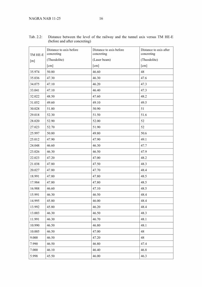
Tab. 2.2: Distance between the level of the railway and the tunnel axis versus TM HE-E (before and after concreting) ............................................................................... 16
Tab. 4.1: Liner specifications................................................................................................. 39
Tab. 4.2: Specification of heaters........................................................................................... 40
Tab. 4.3: Main mechanical characteristics of the heaters ...................................................... 43
Tab. 5.1: Sensors installed in the cross-sections through the microtunnel. ........................... 61
Tab. 5.2: Borehole depths and inclinations for the minipiezometer boreholes – planned and actual values (0° = vertical up, clockwise counting when looking into the microtunnel)...................................................................................................... 68
Tab. 6.1: Laboratory tests of pieces broken of the bentonite blocks (higher water content than intact block) and emplaced granular bentonite (see appendix 4). .... 109
Tab. A.3.1: List of sensors for the HE-E experiment, including the type of sensors, the distance to the tunnel surface or centre of the tunnel and location in PEBS coordinate system ................................................................................................. C-1

NAGRA NAB 11-25 VI
List of Figures
Fig. 1.1: Modelling framework developed for the HE-E experiment within the PEBS project. ...................................................................................................................... 2
Fig. 2.1: Location of HE-E test section (inside the RB microtunnel and in the former VE test section)......................................................................................................... 3
Fig. 2.2: Geological mapping of the test section from MTM 55,55 to MT 45,55. ................. 4
Fig. 2.3: Conceptual lay-out of the HE-E experiment............................................................. 6
Fig. 2.4: Lay-out of the HE-E experiment. ............................................................................. 7
Fig. 2.5: MI niche layout [mm]............................................................................................... 7
Fig. 2.6: MI niche and microtunnel access ............................................................................. 8
Fig. 2.7: RB microtunnel initial conditions as observed on April 2010 [m]........................... 9
Fig. 2.8: 3D image of the VE test section (from TM HE-E 26.5 – TM HE-E 36.5) before the emplacement of the HE-E experiment (data from Flotron, 2010). ........ 10
Fig. 2.9: Microtunnel cleanup phase before initiating activities for the HE-E experiment showing the presence of the steel rings hindering the emplacement of the railway system (font from Solexperts). .................................. 11
Fig. 2.10: Replacement of the steel rings (those in front have been replaced) to permit the emplacement of the railway system (picture from Swisstopo). ........................ 11
Fig. 2.11: Tracing marks in microtunnel for the position of plug #3 (TM HE-E 27.18), the reference section SA3 (TM HE-E 31.48) and the position of plug #1 (TM HE-E 35.78)............................................................................................................ 14
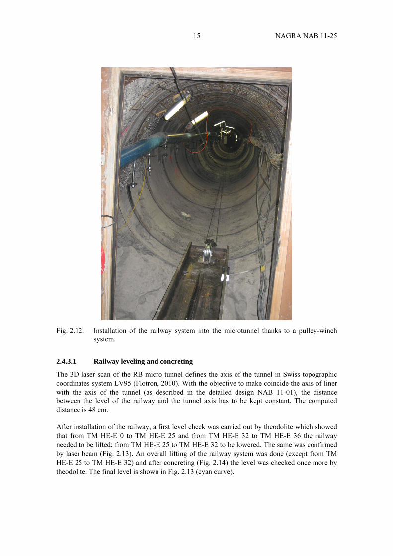
Fig. 2.12: Installation of the railway system into the microtunnel thanks to a pulley-winch system. ......................................................................................................... 15
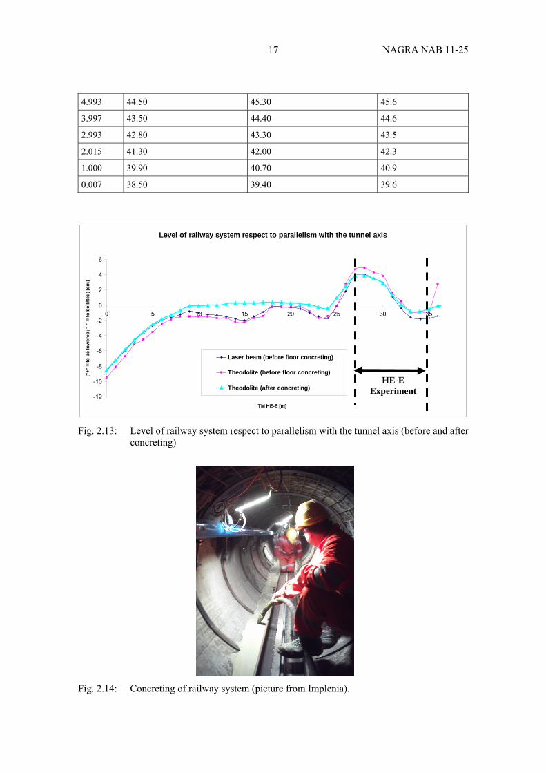
Fig. 2.13: Level of railway system respect to parallelism with the tunnel axis (before and after concreting) ............................................................................................... 17
Fig. 2.14: Concreting of railway system (picture from Implenia). ......................................... 17
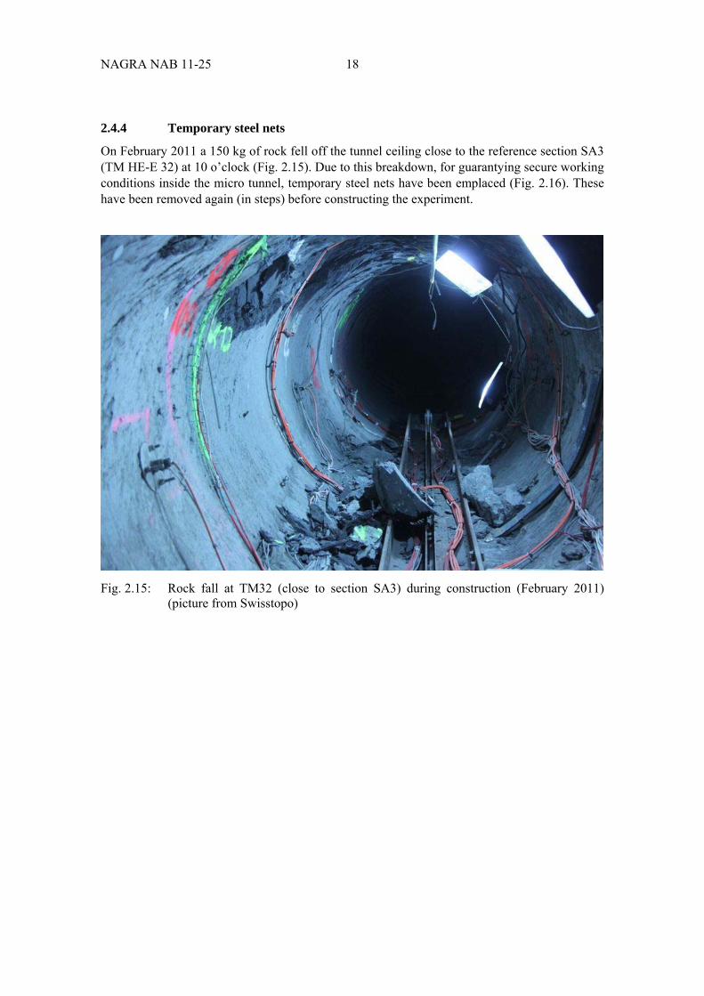
Fig. 2.15: Rock fall at TM32 (close to section SA3) during construction (February 2011) (picture from Swisstopo) .............................................................................. 18
Fig. 2.16: Emplacement of temporary steel nets (picture from Swisstopo) ........................... 19
Fig. 3.1: Lay-out of the HE-E experiment. ........................................................................... 21
Fig. 3.2: Dimensions of bentonite blocks used for the HE-E experiment............................. 21
Fig. 3.3: Sticking capacity of two bentonite blocks by moisturing the connected surface (provided by Alpha Ceramics, Germany). ................................................. 22
Fig. 3.4: Block general view (photo by IGT – ETH Zurich) ................................................ 23
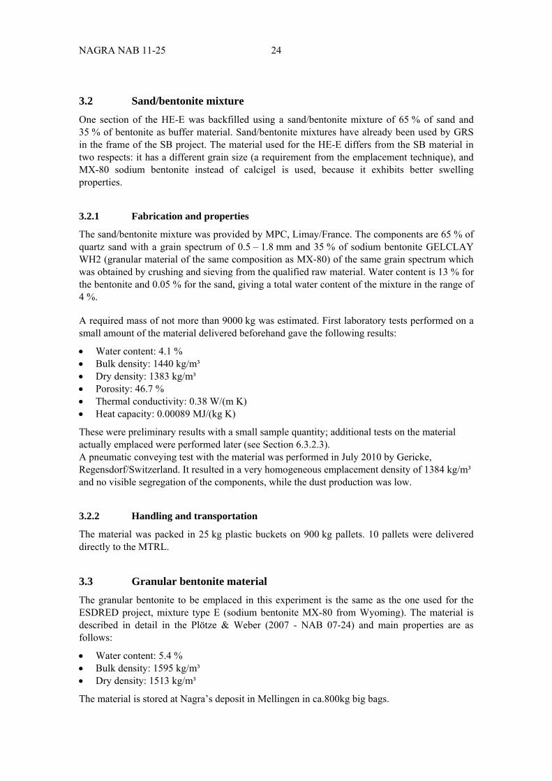
Fig. 3.5: Layout of the emplacement machine and of the pre-test set-up at Hagerbach Test Gallery Ltd...................................................................................................... 27
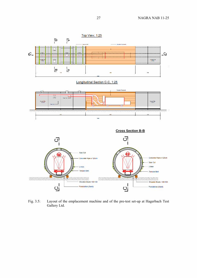
Fig. 3.6: a) Concrete tube elements; b) workers during emplacement operations within the wooden casing; c) emplacement device (auger system); d) hand rammers placed sidewise along the auger. ............................................................................ 28
VII NAGRA NAB 11-25
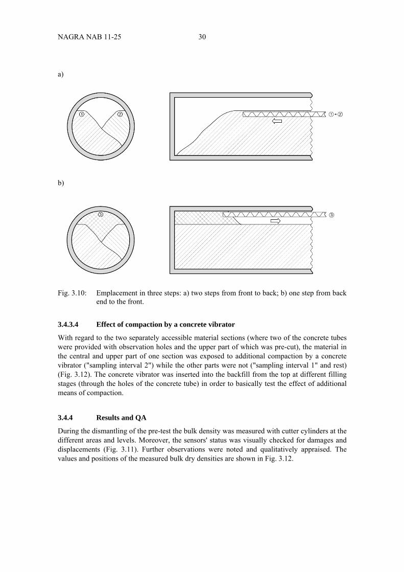
Fig. 3.10: Emplacement in three steps: a) two steps from front to back; b) one step from back end to the front. ..................................................................................... 30
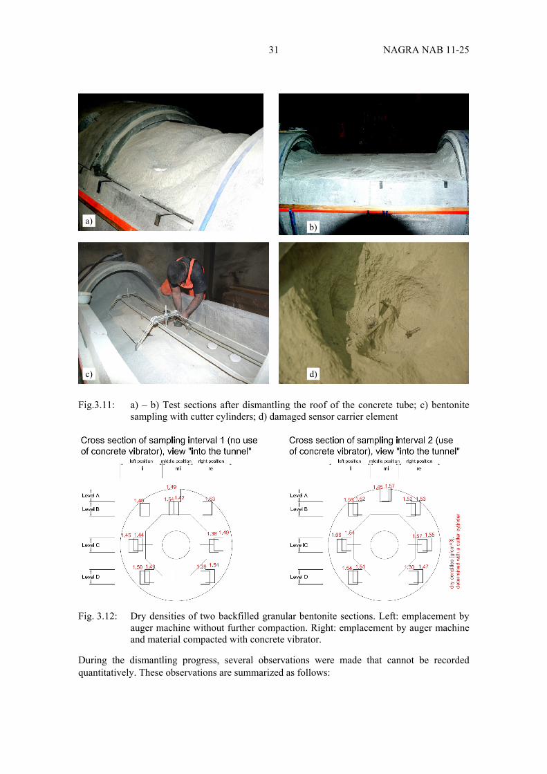
Fig.3.11: a) – b) Test sections after dismantling the roof of the concrete tube; c) bentonite sampling with cutter cylinders; d) damaged sensor carrier element ....... 31
Fig. 3.12: Dry densities of two backfilled granular bentonite sections. Left: emplacement by auger machine without further compaction. Right: emplacement by auger machine and material compacted with concrete vibrator.................................................................................................................... 31
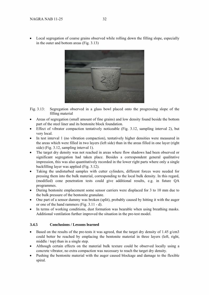
Fig. 3.13: Segregation observed in a glass bowl placed onto the progressing slope of the filling material .................................................................................................. 32
Fig. 3.14: Cement bricks type Z 12......................................................................................... 34
Fig. 3.15: Cement mortar type M15 (Maxit 920).................................................................... 34
Fig. 3.16: Rockwoll (SPACEROCK RSK 830 and PARA) by FLUMROC AG. .................. 35
Fig. 3.17: Vapour barrier (TECHNONORM) by KORFF AG. .............................................. 35
Fig. 4.1: Layout of electrical heaters for HE-E experiment. ................................................. 37
Fig. 4.2: Liner configuration ................................................................................................. 38
Fig. 4.3: Dimensions of MI niche ......................................................................................... 40
Fig. 4.4: Schematic of the heater construction ...................................................................... 43
Fig. 4.5: Arrangement of external thermocouples................................................................. 46
Fig. 4.6: Schematic of the power regulation unit. ................................................................. 49
Fig. 5.1: Technical drawing of the HS-Sensor arms and location of the sensors on the arms, in the bentonite blocks and at the interface between the engineered barrier and the OPA hostrock. ................................................................................ 57
Fig. 5.2: 3D representation of the modules consisting of the instrumentation rings, the bentonite blocks and the steel base slide (the liner element is not shown)............. 58
Fig. 5.3: Technical drawing of the 3 connected modules for one of the sections and the location of the instrumentation arms with respect to the plugs......................... 59
Fig. 5.4: Clarification of the sensor nomenclature in the engineered barrier. ...................... 60
Fig. 5.5: Location of the instrumentation cross sections in the Opalinus clay and their position with respect to the HE-E experiment ........................................................ 61
Fig. 5.6: Generalized 3D drawing of Solexperts Mini-Piezometer System. ......................... 63
Fig. 5.7: Mini-extensometer layout....................................................................................... 64
Fig. 5.8: Representative photo of the capacitive humidity sensor. ....................................... 64
Fig. 5.9: Schematic drawing of the psychrometer type relative humidity sensors................ 66
Fig. 5.10: GRS minipiezometer (left), coaxial tubing (center), valve panel with gauge and transducer (right).............................................................................................. 67
Fig. 5.11: Sensor types and locations in Section SA1 (distances indicated are with respect to the microtunnel wall). ............................................................................ 69
Fig. 5.12: Sensor types and locations in Section SA2 (distances indicated are with respect to the microtunnel wall). ............................................................................ 69
NAGRA NAB 11-25 VIII
Fig. 5.13: Sensor types and locations in Section SA3 (distances indicated are with respect to the microtunnel wall). ............................................................................ 70
Fig. 5.14: Sensor types and locations in Section SA4 (distances indicated are with respect to the microtunnel wall). ............................................................................ 70
Fig. 5.15: Sensor types and locations in Section SB1 (distances indicated are with respect to the microtunnel wall). ............................................................................ 71
Fig. 5.16: Sensor types and locations in Section SB2 (distances indicated are with respect to the microtunnel wall). ............................................................................ 71
Fig. 5.17: Sensor types and locations in Section SD1 (distances indicated are with respect to the microtunnel wall). ............................................................................ 72
Fig. 5.18: Sensor types and locations in Section SD2 (distances indicated are with respect to the microtunnel wall). ............................................................................ 72
Fig. 5.19: Location of borehole BVE-1 and distances of the pore pressure sensors to the microtunnel. ...................................................................................................... 73
Fig. 5.20: Location of borehole BVE-91 and distances of the pore pressure sensors to the microtunnel. ...................................................................................................... 73
Fig. 5.21: Plan view showing the locations of the boreholes BVE-1, BVE-91, BHE-E1, and BHE-E2............................................................................................................ 74
Fig. 5.22: Quadruple packer probe as installed in boreholes BHE-E1 and BHE-E2. ............. 75
Fig. 5.23: Location of boreholes BHE-E1 and BHE-E2 and distances of the test intervals to the microtunnel. ................................................................................... 75
Fig. 5.24: Location and general layout of the seismic transmission experiment in the HE-E micro tunnel.................................................................................................. 76
Fig. 5.25: Layout of the seismic array used for the seismic transmission experiment............ 77
Fig. 5.26: Three piezoelectric transducers just after the installation (emitter B, receivers 1 and 5, see Fig. 5.25) close to the tunnel wall which will be covered later by the sand-bentonite mixture. .................................................................................... 78
Fig. 5.27: Seismic section (raw data) of emitter B and receiver 6 (see Fig. 5.25). Emplacement of buffer material started on May 2nd, 2011 (day 52). .................... 79
Fig. 5.28: Geoelectric array around the VE microtunnel. Left: Installation of surface electrodes, Right: layout of complete electrode array. ........................................... 80
Fig. 5.29: Cross section through an electrode borehole (a rubber tube was added to provide a spring coupling of the electrodes)........................................................... 81
Fig. 5.30: Principle configuration of a dipole-dipole measurement........................................ 82
Fig. 5.31: RESECS measuring system (left) and decoder boxes (right). ................................ 83
Fig. 6.1: Location of the reference section (SA3). ................................................................ 88
Fig. 6.2: Plug #1: as built. ..................................................................................................... 90
Fig. 6.3: Plug #1 as completed. ............................................................................................. 91
Fig. 6.4: Plug #2: as built. ..................................................................................................... 92
Fig. 6.5: Plug #2: (a) First wall as completed; (b) application of isolation system and vapour barrier; (c) second wall as completed. ........................................................ 93
IX NAGRA NAB 11-25
Fig. 6.6: Plug #3: as built. ..................................................................................................... 94
Fig. 6.7: Plug #3: (a) dying end scaffolding wall for concrete block; (b) concrete block; (c) last wall as completed. ........................................................................... 95
Fig. 6.8: Renovated module rack and read-out rack for the humidity sensors (left); PC rack for the Geomonitor (right). ............................................................................. 96
Fig. 6.9: Installation of the humidity sensors (left) and emplacement of the cables in the cable shaft (right). ............................................................................................. 97
Fig. 6.10: Construction of the instrumentation modules on the platform. .............................. 97
Fig. 6.11: Completed Nagra modules on the platform (left) and after towing in the microtunnel. ............................................................................................................ 98
Fig. 6.12: GRS section before emplacement of the modules (left) and completion of the modules on the platform (right) (Pictures: Comet)................................................. 99
Fig. 6.13: (Top) Shifted position of the sensors in the bentonite blocks in the GRS section. (B ottom) Establishment of the position of the centre of the liner with respect to the theoretical axis at the location of the six instrumentation arms based on the position of the railway and the height of the blocks. .............. 100
Fig. 6.14: Failure modes of bentonite blocks. ....................................................................... 102
Fig. 6.15: Construction of the first wall of plug #2 as fixed support of the liner.................. 103
Fig. 6.16: (a) auger machine used for buffer material emplacement; (b) flexible auger conveyor; (c) loading phase of the auger machine on the railway by forklift truck; (d) second auger machine used to transport the buffer material from the ground level of the MI niche till the level of the railway; (e) delivery of buffer material in big bags; (f) filling of the drum mixer; (g) – (h) drum mixer is ready to be pushed into the microtunnel for delivery of the buffer material. ................................................................................................................ 105
Fig. 6.17: Filling sequence of the bentonite section.............................................................. 106
Fig. 6.18: (a) – (l) bentonite filling operations...................................................................... 108
Fig. 6.19: Bentonite section (TM HE-E 31.73 - TM HE-E 35.78) ...................................... 110
Fig. 6.20: Laser scan of the sand/bentonite section (TM HE-E 27.18 - TM HE-E 31.18).................................................................................................................... 111
Fig. 6.21: Liner, bentonite blocks, and instrumentation in the sand/bentonite section. ........ 111
Fig. 6.22: Sand/bentonite filling equipment.......................................................................... 112
Fig. 6.23: Start of sand/bentonite emplacement.................................................................... 112
Fig. 6.24: Sand/bentonite emplacement. ............................................................................... 113
Fig. 6.25: Sand/bentonite section shortly before finishing backfilling. On the right: Shuffle for filling the roof gap.............................................................................. 113
Fig. 6.26: Sand/bentonite sample preparation....................................................................... 114
Fig. 6.27: Sand/bentonite samples. ....................................................................................... 115
Fig. 6.28: a) Power cabinets; b) traction cable inspection. ................................................... 117
Fig. 6.29: a) Heater 2 on the MI niche platform; b) detail of the thermocouples positioning pieces. ................................................................................................ 118
NAGRA NAB 11-25 X
Fig. 6.30: a) Heater 2 at the liner entrance; b) Heater 2 partially introduced inside the liner....................................................................................................................... 118
Fig. 6.31: a) Heater 1 at the microtunnel entrance; b) corrugated tube (floor) and auxiliary rod.......................................................................................................... 119
Fig. 6.32: a) Cables from heater 2 entering in heater 1. b) Detail of the PPS tube connecting heater 1 and heater 2. ......................................................................... 119
Fig. 6.33: a) Insertion operation; b) hoist installed at the microtunnel entry. ....................... 120
Fig. 6.34: Final disposition of heaters: a) Heater 1; b) heater 2. ........................................... 120
Fig. 6.35: a) DAS compartment; b) power cabinets final disposition................................... 121
Fig. 6.36: Detailed of the pulley and the twisted traction cable............................................ 121
Fig. 7.1: Heating steps for the HE-E experiment (indicated by the multi-coloured line)....................................................................................................................... 123
1 NAGRA NAB 11-25
1 Introduction and objectives
1.1 Context of the experiment
The evolution of the engineered barrier system (EBS) of geological repositories for radioactive waste has been the subject of many national and international research programmes during the last decade. The emphasis of the research activities was on the elaboration of a detailed understanding of the complex THM-C processes, which are expected to evolve in the early post closure period in the near field. From the perspective of radiological long-term safety, an in depth understanding of these coupled processes is of great significance, because the evolution of the EBS during the early post-closure phase may have a non-negligible impact on the radiological safety functions at the time when the canisters breach. Unexpected process interactions during the saturation phase (heat pulse, gas generation, non-uniform water uptake from the host rock) could impair the homogeneity of the safety-relevant parameters in the EBS (e.g. swelling pressure, hydraulic conductivity, diffusivity).
In previous EU-supported research programmes such as FEBEX, ESDRED and NFPRO, remarkable advances have been made to broaden the scientific understanding of THM-C coupled processes in the near field around the waste canisters. The experimental data bases were extended on the laboratory and field scale and numerical simulation tools were developed. Less successful, however, was the attempt to use this in-depth process understanding for constraining the conceptual and parametric uncertainties in the context of long-term safety assessment. It was recognised that Performance Assessment (PA)-related uncertainties could not be reduced significantly with the newly developed THM-C codes due to a lack of confidence in their predictive capabilities on time scales which are relevant for PA.
The 7th Framework PEBS project (Long Term Performance of Engineered Barrier Systems) is addressing this issue. Specifically, the HE-E experiment, as part of PEBS, is expected to provide a good quality experimental TH and THM database for the model validation process and will thus allow evaluating the key thermo-hydro-mechanical processes and parameters taking place during the early evolution of the EBS.
1.2 Objectives of the experiment
The main objectives of the HE-E experiment are:
to provide the experimental data base required for the calibration and validation of existing thermo-hydraulic models of the early saturation phase of the buffer
to upscale thermal conductivity of the partially saturated buffer from the laboratory to the field scale (for pure bentonite and bentonite-sand mixtures).
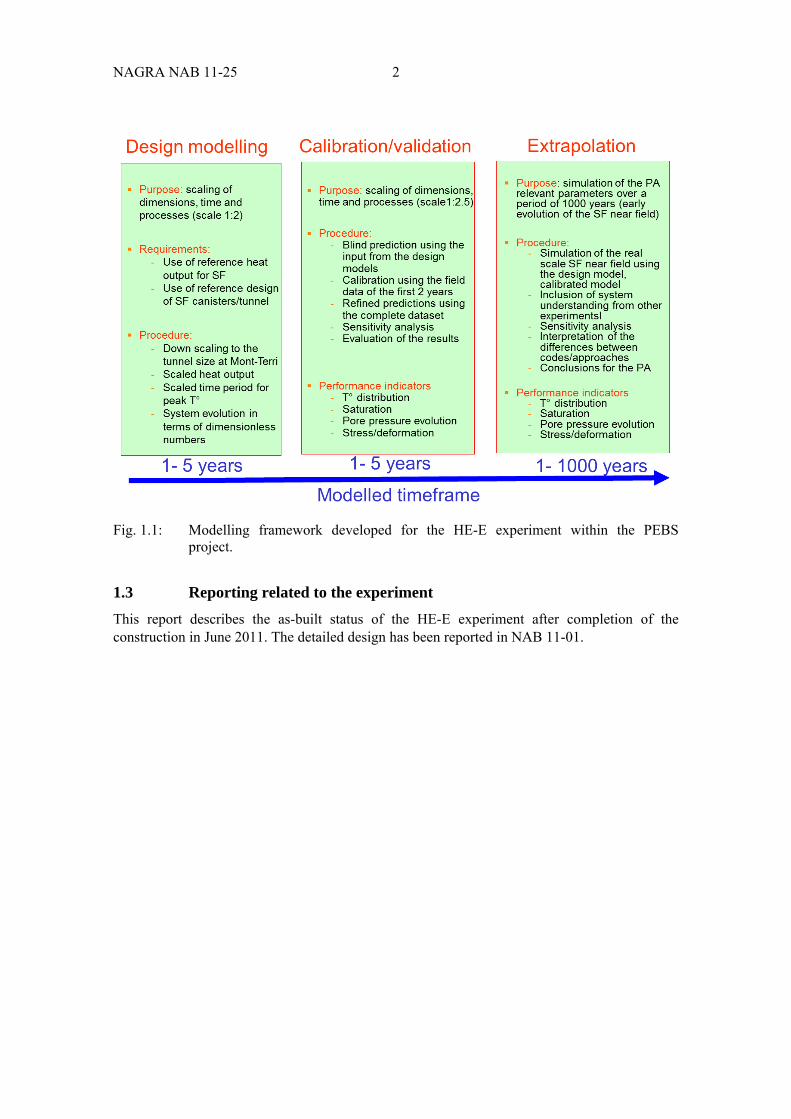
The HE-E experiment is primarily a validation experiment at the large scale, but has also certain aspects of a demonstration experiment. The modelling of the experiment forms an essential part of the PEBS project (WP3) and consist of three stages (Fig. 1.1) namely design modelling, calibration and prediction/validation and the extrapolation. The design of the experiment and the way it is conducted should therefore be such that data resolution is optimised and processes can be distinguished and observed individually.
NAGRA NAB 11-25 2
Fig. 1.1: Modelling framework developed for the HE-E experiment within the PEBS project.
1.3 Reporting related to the experiment
This report describes the as-built status of the HE-E experiment after completion of the construction in June 2011. The detailed design has been reported in NAB 11-01.
3 NAGRA NAB 11-25
2 Location and general layout of the experiment
The HE-E experiment is constructed in the former VE test section, located in the RB micro tunnel of the Mont Terri Rock Laboratory.
2.1 Characteristics of VE test section
The detailed characterisation of the VE test section occurred as part of the previous VE experiment (Mayor et al., 2007) and is included again for clarity below.
2.1.1 Location and geometry
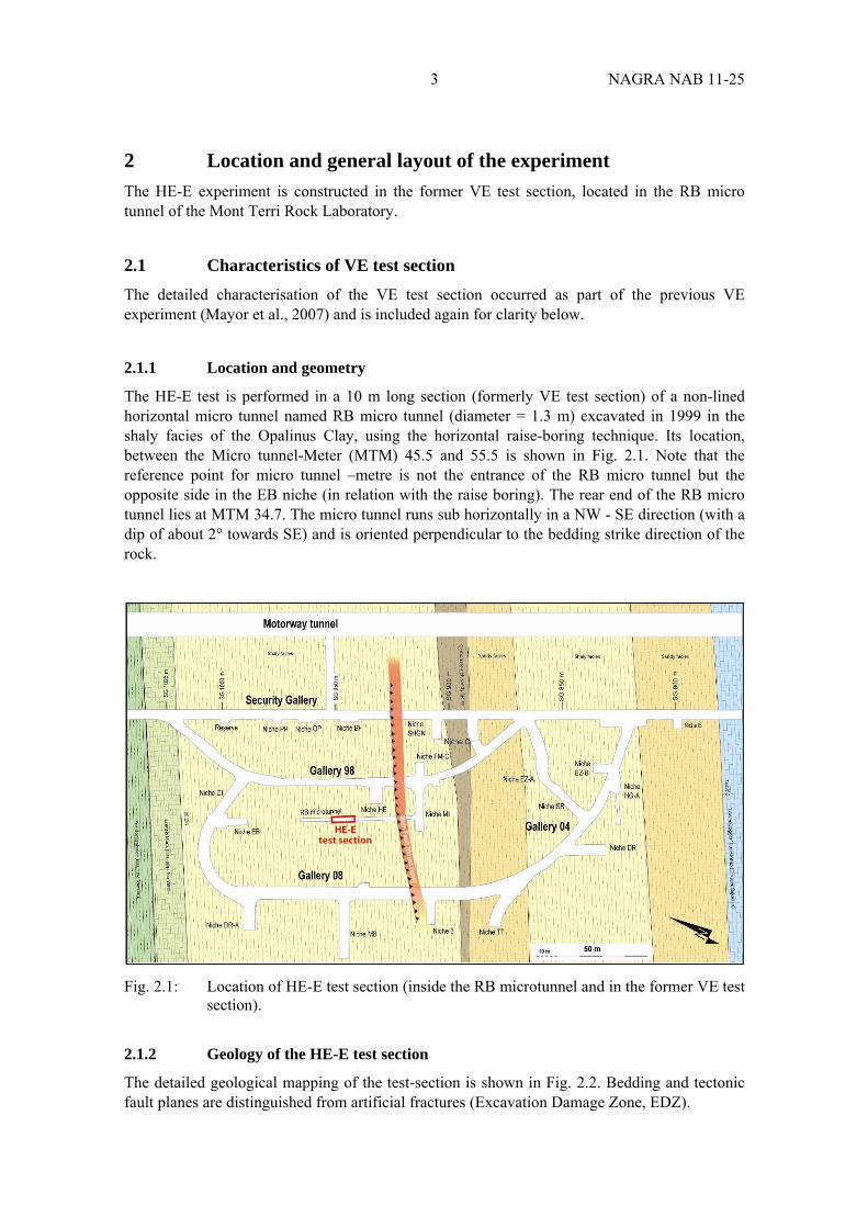
The HE-E test is performed in a 10 m long section (formerly VE test section) of a non-lined horizontal micro tunnel named RB micro tunnel (diameter = 1.3 m) excavated in 1999 in the shaly facies of the Opalinus Clay, using the horizontal raise-boring technique. Its location, between the Micro tunnel-Meter (MTM) 45.5 and 55.5 is shown in Fig. 2.1. Note that the reference point for micro tunnel –metre is not the entrance of the RB micro tunnel but the opposite side in the EB niche (in relation with the raise boring). The rear end of the RB micro tunnel lies at MTM 34.7. The micro tunnel runs sub horizontally in a NW - SE direction (with a dip of about 2° towards SE) and is oriented perpendicular to the bedding strike direction of the rock.
Fig. 2.1: Location of HE-E test section (inside the RB microtunnel and in the former VE test section).
2.1.2 Geology of the HE-E test section
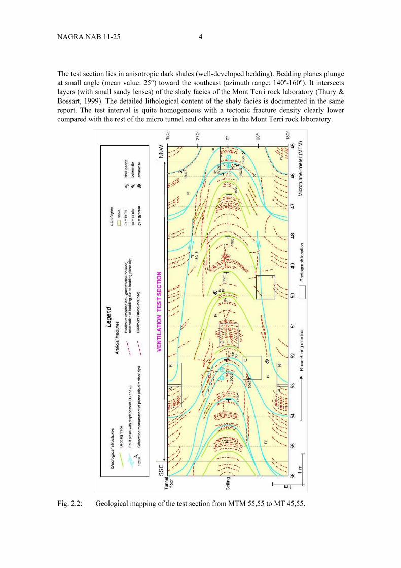
The detailed geological mapping of the test-section is shown in Fig. 2.2. Bedding and tectonic fault planes are distinguished from artificial fractures (Excavation Damage Zone, EDZ).
NAGRA NAB 11-25 4
The test section lies in anisotropic dark shales (well-developed bedding). Bedding planes plunge at small angle (mean value: 25°) toward the southeast (azimuth range: 140º-160º). It intersects layers (with small sandy lenses) of the shaly facies of the Mont Terri rock laboratory (Thury & Bossart, 1999). The detailed lithological content of the shaly facies is documented in the same report. The test interval is quite homogeneous with a tectonic fracture density clearly lower compared with the rest of the micro tunnel and other areas in the Mont Terri rock laboratory.
Fig. 2.2: Geological mapping of the test section from MTM 55,55 to MT 45,55.
5 NAGRA NAB 11-25
Bedding planes are sub-parallel or dip at a lower angle than the fault planes, which show slicken sides and fibres on polished surfaces, with a sense of shear that consistently indicates over thrusting towards the NNW. A sub horizontal fault plane cuts the micro tunnel floor at about MTM 53 and is hidden from MTM 48,5. The internal structure of the Mont Terri anticline may be explained by a thrust system of a flat-ramp system which is also developed at smaller scale within the Opalinus Clay. Structures may be described as small imbricate sheets with flat thrust levels and ramps which cut through the bedding planes. The whole structure had passively rotated during the folding of the Mont Terri anticline. This would explain the unusually steep angles of some thrust planes (> 30°).
Basically, there are two types of damage structures related to underground openings in the Opalinus Clay: 1) extension fracturing due to stress re-distributions (unloading joints), 2) brittle reactivation of bedding planes and tectonic fractures. Structures of type 2 were mapped in detail within the test section (Fig. 2.2), together with breakouts. The extension fractures (type 1) cannot be directly observed in the micro tunnel because there are no lateral niches and thus, no perpendicular sections. These fractures are present at the entrance of the micro tunnel in the walls of the MI niche. An artificial fracture network developed at the top and bottom of the micro tunnel with slip reactivation of bedding planes and tectonic fault planes. Bedding plane slip seems not only restricted to the top and bottom of the micro tunnel but was also active along the tunnel walls (along 270° line, Fig. 2. 2). This slip direction towards the tunnel may be enhanced by not visible extension fractures.
After the excavation work, small breakouts developed in the ceiling of the micro tunnel. The maximum dimension of such breakouts (wedge-shaped) is in the range of 2 dm3. These breakouts were intensified after closure of the micro tunnel in December 2001, indicating an increase of dip-slip movements along bedding planes due to higher relative humidity.
On both side walls of the micro tunnel (270° and 90° lines, Fig. 2.2), additional breakouts were observed. They could be observed between MTM 46 and MTM 50 and between MTM 52 and MTM 55, respectively. They are indicated in the map of Fig. 2.2 as sub horizontal, stippled red lines. In any case, breakouts in the test section were rather small when compared to other sections in the rock laboratory. It is estimated that the test section was an ideal and stable place for the test installation work and subsequent long term measurements.
2.2 General layout of the experiment
The experiment HE-E (Fig. 2.3) aims at improving the understanding of the thermal evolution of the near field around a SF/HLW waste container, during the very early phase after emplacement in an approximated 1:2 scale in-situ configuration.
NAGRA NAB 11-25 6
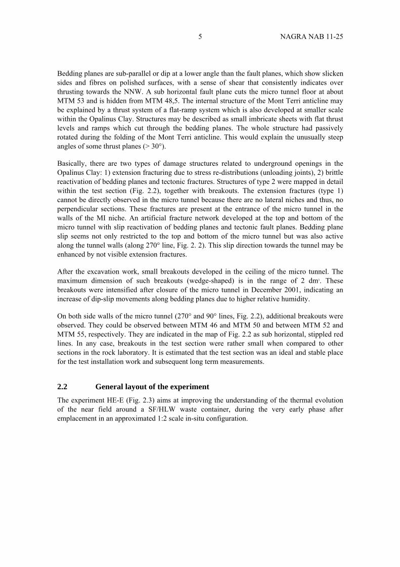
Fig. 2.3: Conceptual lay-out of the HE-E experiment.
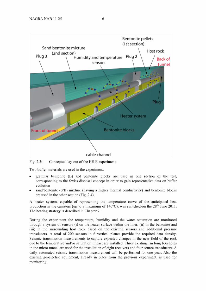
Two buffer materials are used in the experiment:
granular bentonite (B) and bentonite blocks are used in one section of the test, corresponding to the Swiss disposal concept in order to gain representative data on buffer evolution
sand/bentonite (S/B) mixture (having a higher thermal conductivity) and bentonite blocks are used in the other section (Fig. 2.4).
A heater system, capable of representing the temperature curve of the anticipated heat production in the canisters (up to a maximum of 140°C), was switched-on the 28th June 2011. The heating strategy is described in Chapter 7.
During the experiment the temperature, humidity and the water saturation are monitored through a system of sensors (i) on the heater surface within the liner, (ii) in the bentonite and (iii) in the surrounding host rock based on the existing sensors and additional pressure transducers. A total of 200 sensors in 6 vertical planes provide the required data density. Seismic transmission measurements to capture expected changes in the near field of the rock due to the temperature and/or saturation impact are installed. Three existing 1m long boreholes in the micro tunnel are used for the installation of eight receivers and four source transducers. A daily automated seismic transmission measurement will be performed for one year. Also the existing geoelectric equipment, already in place from the previous experiment, is used for monitoring.
7 NAGRA NAB 11-25
Fig. 2.4: Lay-out of the HE-E experiment.
2.3 Description of the initial conditions of the site
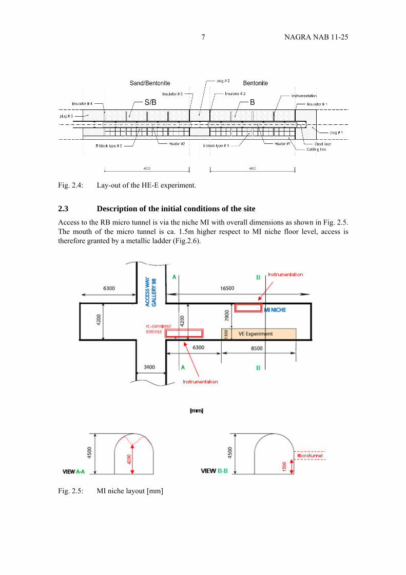
Access to the RB micro tunnel is via the niche MI with overall dimensions as shown in Fig. 2.5. The mouth of the micro tunnel is ca. 1.5m higher respect to MI niche floor level, access is therefore granted by a metallic ladder (Fig.2.6).
Fig. 2.5: MI niche layout [mm]
NAGRA NAB 11-25 8
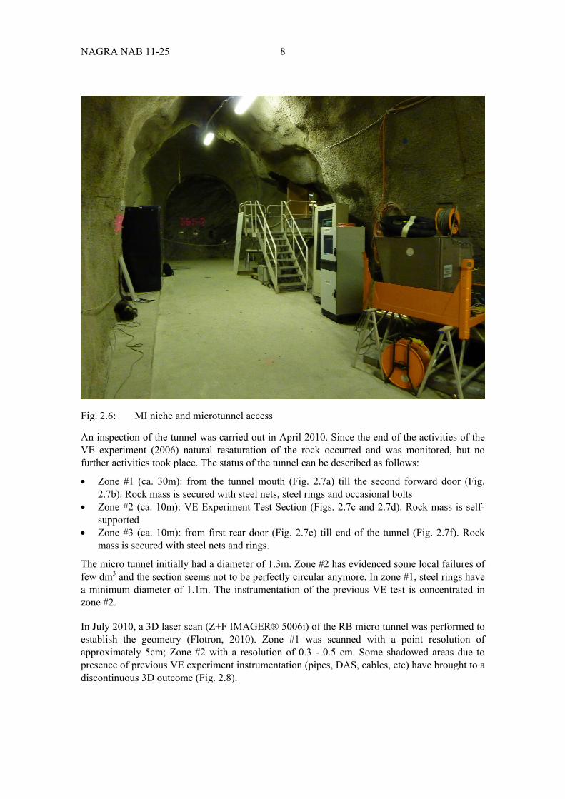
Fig. 2.6: MI niche and microtunnel access
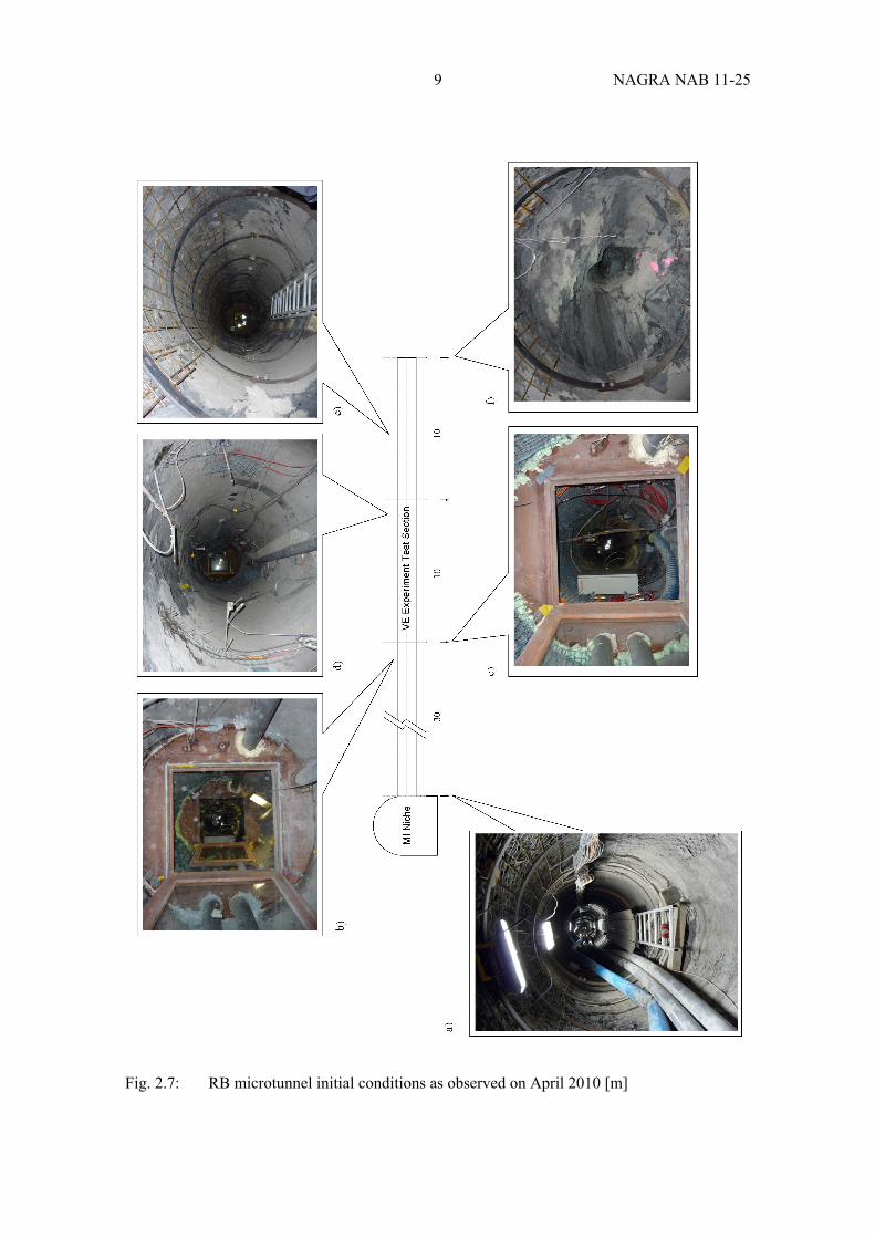
An inspection of the tunnel was carried out in April 2010. Since the end of the activities of the VE experiment (2006) natural resaturation of the rock occurred and was monitored, but no further activities took place. The status of the tunnel can be described as follows:
Zone #1 (ca. 30m): from the tunnel mouth (Fig. 2.7a) till the second forward door (Fig. 2.7b). Rock mass is secured with steel nets, steel rings and occasional bolts
Zone #2 (ca. 10m): VE Experiment Test Section (Figs. 2.7c and 2.7d). Rock mass is self-supported
Zone #3 (ca. 10m): from first rear door (Fig. 2.7e) till end of the tunnel (Fig. 2.7f). Rock mass is secured with steel nets and rings.
The micro tunnel initially had a diameter of 1.3m. Zone #2 has evidenced some local failures of few dm3 and the section seems not to be perfectly circular anymore. In zone #1, steel rings have a minimum diameter of 1.1m. The instrumentation of the previous VE test is concentrated in zone #2.
In July 2010, a 3D laser scan (Z+F IMAGER® 5006i) of the RB micro tunnel was performed to establish the geometry (Flotron, 2010). Zone #1 was scanned with a point resolution of approximately 5cm; Zone #2 with a resolution of 0.3 - 0.5 cm. Some shadowed areas due to presence of previous VE experiment instrumentation (pipes, DAS, cables, etc) have brought to a discontinuous 3D outcome (Fig. 2.8).
9 NAGRA NAB 11-25
Fig. 2.7: RB microtunnel initial conditions as observed on April 2010 [m]

NAGRA NAB 11-25 10
Fig. 2.8: 3D image of the VE test section (from TM HE-E 26.5 – TM HE-E 36.5) before the emplacement of the HE-E experiment (data from Flotron, 2010).
2.4 Site preparation and infrastructure activities
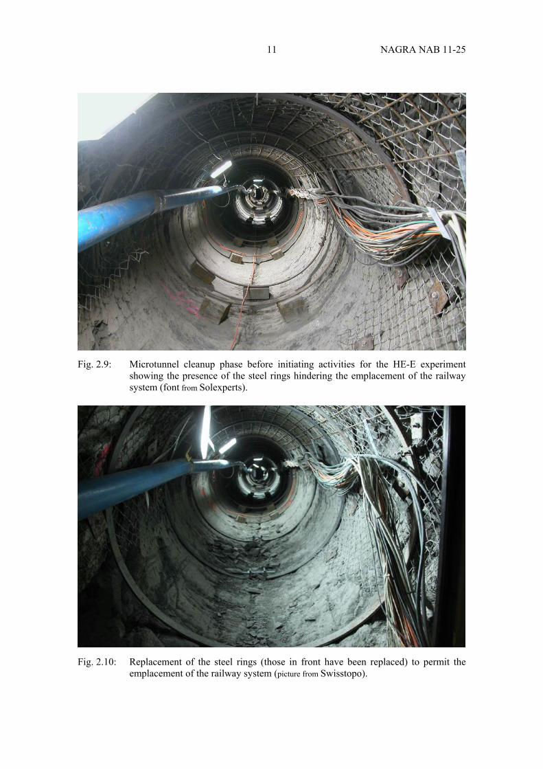
On December 2010, first preparation activities consisted in cleaning up the tunnel by removal of pipes, doors, fixations, wood, loose rock. Loose cables were fixed at the tunnel side walls. 27 steel rings (starting from the tunnel entrance till the end of Zone #1) were substituted with suitable ones which rested directly on the tunnel floor and not on wood blocks as was the case for the existing ones (Figs 2.9 and 2.10).
11 NAGRA NAB 11-25
Fig. 2.9: Microtunnel cleanup phase before initiating activities for the HE-E experiment showing the presence of the steel rings hindering the emplacement of the railway system (font from Solexperts).
Fig. 2.10: Replacement of the steel rings (those in front have been replaced) to permit the emplacement of the railway system (picture from Swisstopo).

NAGRA NAB 11-25 12
2.4.1 Definition of the reference system for the HE-E experiment
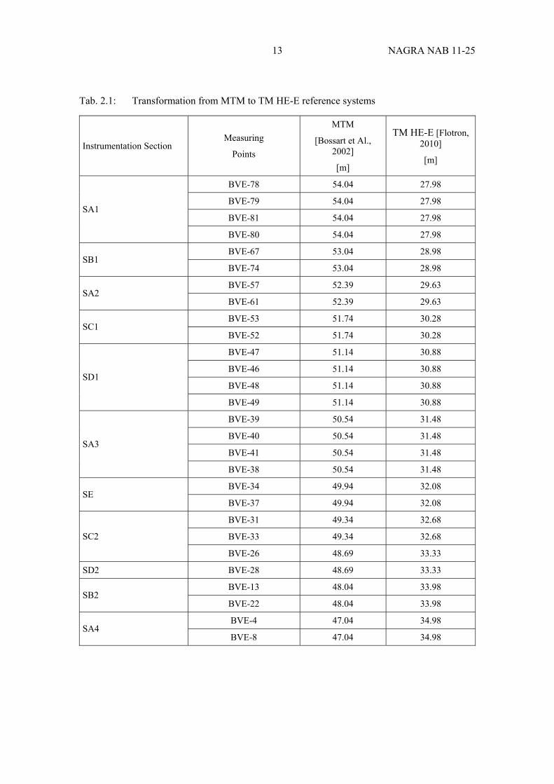
Boreholes and marked control points of the previous VE experiment, referred in Swiss topographic coordinates system LV95 (CH1903+), are listed with the prefix BVE and measured in Micro Tunnel Meter (MTM). This reference system has origin in the EB niche (Bossart et Al., 2002).
For simplifying the construction process of the HE-E experiment, it was decided to define a new reference system with origin closed to the entrance of the RB micro tunnel (Flotron, 2010). Tunnel Meters for the HE-E experiment (TM HE-E) are therefore in opposite direction to MTM (Tab. 2.1). The VE test section located between MTM55.5 – MTM45.5 corresponds to TM HE-E 26.5 – TM HE-E 36.5.
13 NAGRA NAB 11-25
Tab. 2.1: Transformation from MTM to TM HE-E reference systems
Instrumentation Section Measuring
Points
MTM
[Bossart et Al., 2002]
[m]
TM HE-E [Flotron, 2010]
[m]
BVE-78 54.04 27.98
BVE-79 54.04 27.98
BVE-81 54.04 27.98 SA1
BVE-80 54.04 27.98
BVE-67 53.04 28.98 SB1
BVE-74 53.04 28.98
BVE-57 52.39 29.63 SA2
BVE-61 52.39 29.63
BVE-53 51.74 30.28 SC1
BVE-52 51.74 30.28
BVE-47 51.14 30.88
BVE-46 51.14 30.88
BVE-48 51.14 30.88 SD1
BVE-49 51.14 30.88
BVE-39 50.54 31.48
BVE-40 50.54 31.48
BVE-41 50.54 31.48 SA3
BVE-38 50.54 31.48
BVE-34 49.94 32.08 SE
BVE-37 49.94 32.08
BVE-31 49.34 32.68
BVE-33 49.34 32.68 SC2
BVE-26 48.69 33.33
SD2 BVE-28 48.69 33.33
BVE-13 48.04 33.98 SB2
BVE-22 48.04 33.98
BVE-4 47.04 34.98 SA4
BVE-8 47.04 34.98
NAGRA NAB 11-25 14
2.4.2 Location of the HE-E experiment inside RB micro tunnel
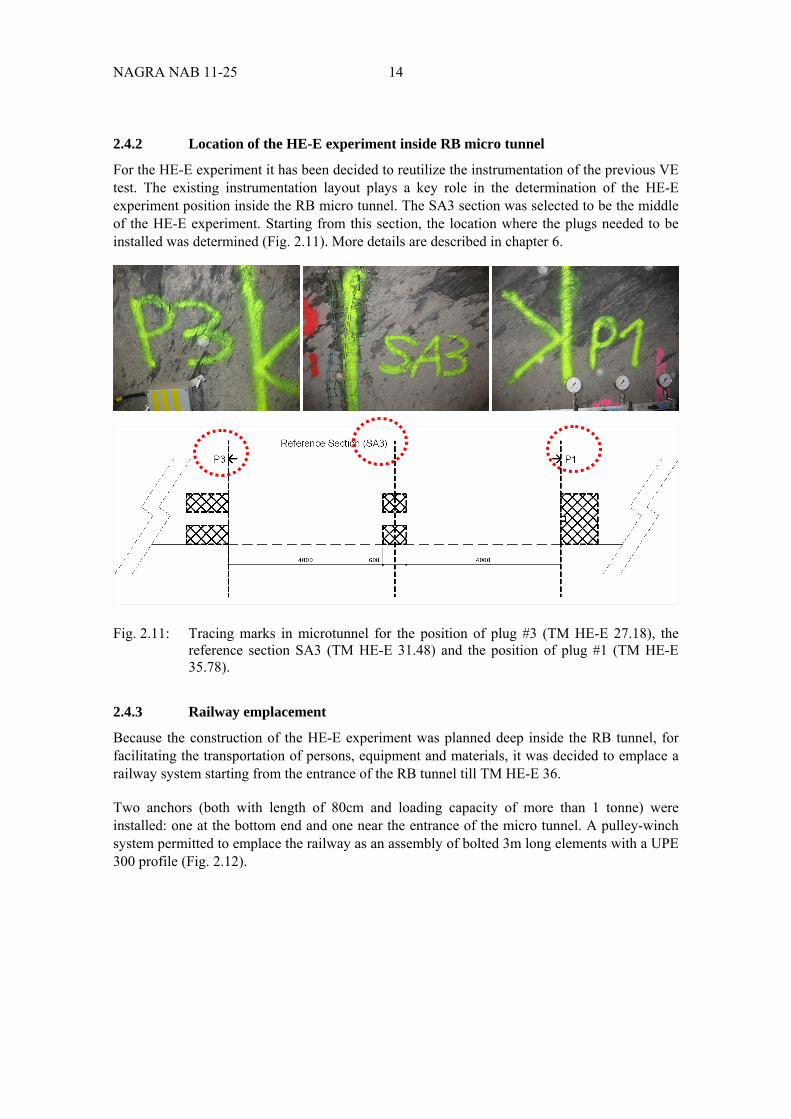
For the HE-E experiment it has been decided to reutilize the instrumentation of the previous VE test. The existing instrumentation layout plays a key role in the determination of the HE-E experiment position inside the RB micro tunnel. The SA3 section was selected to be the middle of the HE-E experiment. Starting from this section, the location where the plugs needed to be installed was determined (Fig. 2.11). More details are described in chapter 6.
Fig. 2.11: Tracing marks in microtunnel for the position of plug #3 (TM HE-E 27.18), the reference section SA3 (TM HE-E 31.48) and the position of plug #1 (TM HE-E 35.78).
2.4.3 Railway emplacement
Because the construction of the HE-E experiment was planned deep inside the RB tunnel, for facilitating the transportation of persons, equipment and materials, it was decided to emplace a railway system starting from the entrance of the RB tunnel till TM HE-E 36.
Two anchors (both with length of 80cm and loading capacity of more than 1 tonne) were installed: one at the bottom end and one near the entrance of the micro tunnel. A pulley-winch system permitted to emplace the railway as an assembly of bolted 3m long elements with a UPE 300 profile (Fig. 2.12).
15 NAGRA NAB 11-25
Fig. 2.12: Installation of the railway system into the microtunnel thanks to a pulley-winch system.
2.4.3.1 Railway leveling and concreting
The 3D laser scan of the RB micro tunnel defines the axis of the tunnel in Swiss topographic coordinates system LV95 (Flotron, 2010). With the objective to make coincide the axis of liner with the axis of the tunnel (as described in the detailed design NAB 11-01), the distance between the level of the railway and the tunnel axis has to be kept constant. The computed distance is 48 cm.
After installation of the railway, a first level check was carried out by theodolite which showed that from TM HE-E 0 to TM HE-E 25 and from TM HE-E 32 to TM HE-E 36 the railway needed to be lifted; from TM HE-E 25 to TM HE-E 32 to be lowered. The same was confirmed by laser beam (Fig. 2.13). An overall lifting of the railway system was done (except from TM HE-E 25 to TM HE-E 32) and after concreting (Fig. 2.14) the level was checked once more by theodolite. The final level is shown in Fig. 2.13 (cyan curve).
NAGRA NAB 11-25 16
Tab. 2.2: Distance between the level of the railway and the tunnel axis versus TM HE-E (before and after concreting)
TM HE-E
[m]
Distance to axis before concreting
(Theodolite)
[cm]
Distance to axis before concreting
(Laser beam)
[cm]
Distance to axis after concreting
(Theodolite)
[cm]
35.974 50.80 46.60 48
35.036 47.30 46.30 47.6
34.075 47.10 46.20 47.3
33.041 47.10 46.40 47.3
32.022 48.50 47.60 48.2
31.052 49.60 49.10 49.5
30.028 51.80 50.90 51
29.018 52.30 51.50 51.6
28.020 52.90 52.00 52
27.023 52.70 51.90 52
25.997 50.80 49.80 50.6
25.012 47.90 47.90 49.1
24.048 46.60 46.30 47.7
23.026 46.30 46.50 47.9
22.023 47.20 47.00 48.2
21.038 47.80 47.50 48.3
20.027 47.80 47.70 48.4
18.991 47.80 47.80 48.5
17.984 47.80 47.80 48.5
16.988 46.60 47.10 48.5
15.991 46.30 46.50 48.4
14.995 45.80 46.00 48.4
13.992 45.80 46.20 48.4
13.003 46.30 46.50 48.3
11.991 46.30 46.70 48.1
10.990 46.50 46.80 48.1
10.005 46.50 47.00 48
9.000 46.50 47.20 48
7.990 46.50 46.80 47.4
7.000 46.10 46.40 46.8
5.998 45.50 46.00 46.3
17 NAGRA NAB 11-25
4.993 44.50 45.30 45.6
3.997 43.50 44.40 44.6
2.993 42.80 43.30 43.5
2.015 41.30 42.00 42.3
1.000 39.90 40.70 40.9
0.007 38.50 39.40 39.6
Fig. 2.13: Level of railway system respect to parallelism with the tunnel axis (before and after concreting)
Fig. 2.14: Concreting of railway system (picture from Implenia).
Level of railway system respect to parallelism with the tunnel axis
-12
-10
-8
-6
-4
-2
0
2
4
6
0 5 10 15 20 25 30 35
TM HE-E [m]
("+
" =
to b
e lo
we
red
; "-
" =
to b
e li
fted
) [cm
]
Laser beam (before floor concreting)
Theodolite (before floor concreting)
Theodolite (after concreting)HE-E
Experiment
NAGRA NAB 11-25 18
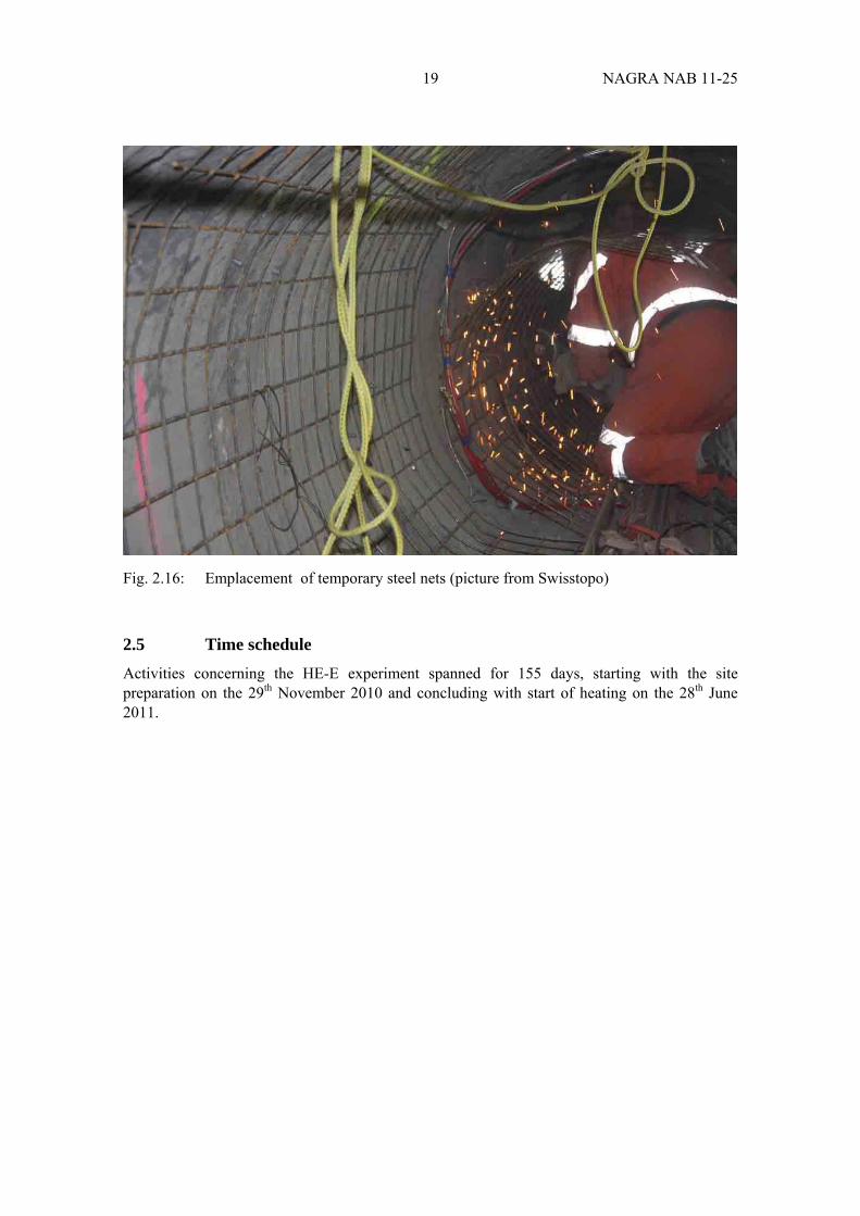
2.4.4 Temporary steel nets
On February 2011 a 150 kg of rock fell off the tunnel ceiling close to the reference section SA3 (TM HE-E 32) at 10 o’clock (Fig. 2.15). Due to this breakdown, for guarantying secure working conditions inside the micro tunnel, temporary steel nets have been emplaced (Fig. 2.16). These have been removed again (in steps) before constructing the experiment.
Fig. 2.15: Rock fall at TM32 (close to section SA3) during construction (February 2011) (picture from Swisstopo)
19 NAGRA NAB 11-25
Fig. 2.16: Emplacement of temporary steel nets (picture from Swisstopo)
2.5 Time schedule
Activities concerning the HE-E experiment spanned for 155 days, starting with the site preparation on the 29th November 2010 and concluding with start of heating on the 28th June 2011.

21 NAGRA NAB 11-25
3 Materials and methods
In this chapter all materials used for the construction of the HE-E experiment including the description of the method for the emplacement of the buffer materials are presented. For clarity the overall lay-out is shown again in Fig. 3.1.
Fig. 3.1: Lay-out of the HE-E experiment.
3.1 Bentonite blocks
Bentonite blocks of sodium bentonite (MX-80) from Wyoming are used for both bentonite and sand/bentonite sections of the experiment.
3.1.1 Design and fabrication
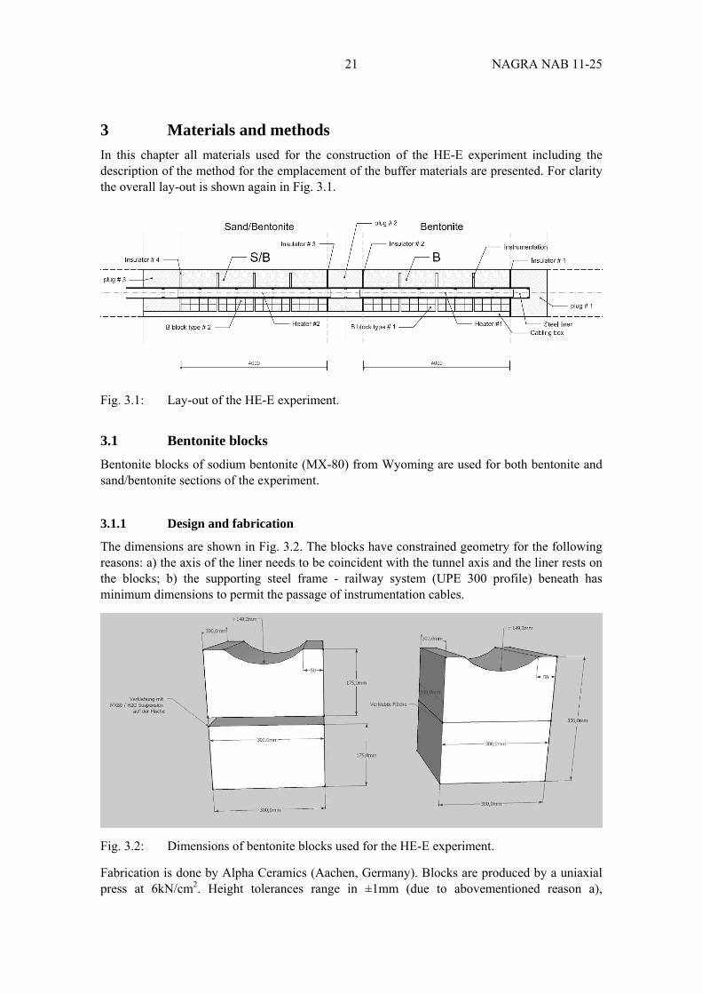
The dimensions are shown in Fig. 3.2. The blocks have constrained geometry for the following reasons: a) the axis of the liner needs to be coincident with the tunnel axis and the liner rests on the blocks; b) the supporting steel frame - railway system (UPE 300 profile) beneath has minimum dimensions to permit the passage of instrumentation cables.
Fig. 3.2: Dimensions of bentonite blocks used for the HE-E experiment.
Fabrication is done by Alpha Ceramics (Aachen, Germany). Blocks are produced by a uniaxial press at 6kN/cm2. Height tolerances range in ±1mm (due to abovementioned reason a),
NAGRA NAB 11-25 22
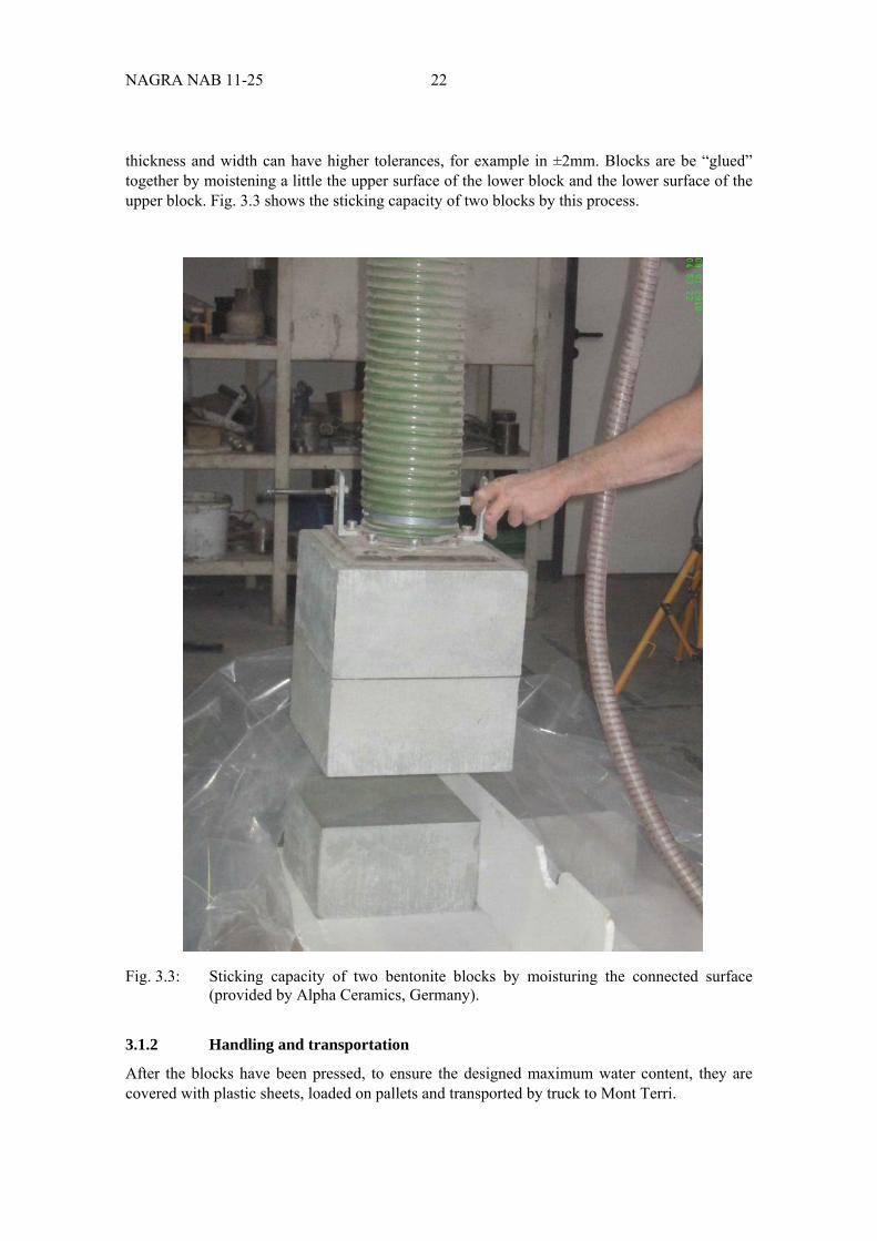
thickness and width can have higher tolerances, for example in ±2mm. Blocks are be “glued” together by moistening a little the upper surface of the lower block and the lower surface of the upper block. Fig. 3.3 shows the sticking capacity of two blocks by this process.
Fig. 3.3: Sticking capacity of two bentonite blocks by moisturing the connected surface (provided by Alpha Ceramics, Germany).
3.1.2 Handling and transportation
After the blocks have been pressed, to ensure the designed maximum water content, they are covered with plastic sheets, loaded on pallets and transported by truck to Mont Terri.
23 NAGRA NAB 11-25
3.1.3 Laboratory tests
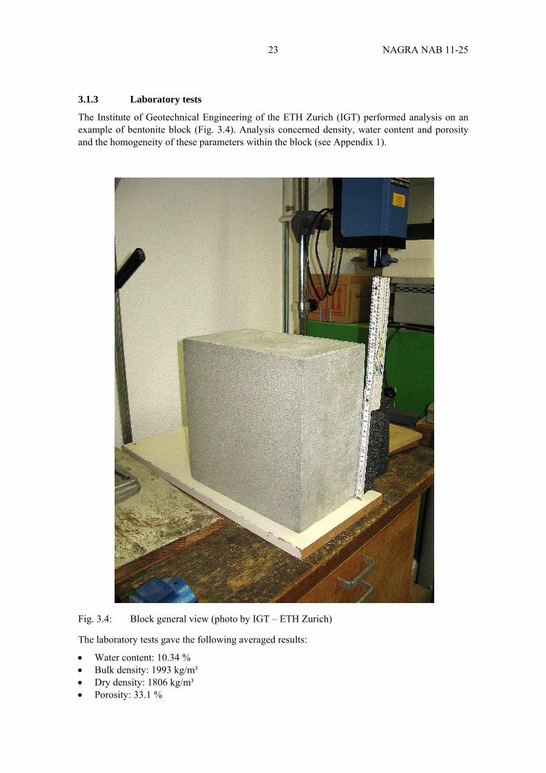
The Institute of Geotechnical Engineering of the ETH Zurich (IGT) performed analysis on an example of bentonite block (Fig. 3.4). Analysis concerned density, water content and porosity and the homogeneity of these parameters within the block (see Appendix 1).
Fig. 3.4: Block general view (photo by IGT – ETH Zurich)
The laboratory tests gave the following averaged results:
Water content: 10.34 % Bulk density: 1993 kg/m³ Dry density: 1806 kg/m³ Porosity: 33.1 %
NAGRA NAB 11-25 24
3.2 Sand/bentonite mixture
One section of the HE-E was backfilled using a sand/bentonite mixture of 65 % of sand and 35 % of bentonite as buffer material. Sand/bentonite mixtures have already been used by GRS in the frame of the SB project. The material used for the HE-E differs from the SB material in two respects: it has a different grain size (a requirement from the emplacement technique), and MX-80 sodium bentonite instead of calcigel is used, because it exhibits better swelling properties.
3.2.1 Fabrication and properties
The sand/bentonite mixture was provided by MPC, Limay/France. The components are 65 % of quartz sand with a grain spectrum of 0.5 – 1.8 mm and 35 % of sodium bentonite GELCLAY WH2 (granular material of the same composition as MX-80) of the same grain spectrum which was obtained by crushing and sieving from the qualified raw material. Water content is 13 % for the bentonite and 0.05 % for the sand, giving a total water content of the mixture in the range of 4 %.
A required mass of not more than 9000 kg was estimated. First laboratory tests performed on a small amount of the material delivered beforehand gave the following results:
Water content: 4.1 % Bulk density: 1440 kg/m³ Dry density: 1383 kg/m³ Porosity: 46.7 % Thermal conductivity: 0.38 W/(m K) Heat capacity: 0.00089 MJ/(kg K)
These were preliminary results with a small sample quantity; additional tests on the material actually emplaced were performed later (see Section 6.3.2.3). A pneumatic conveying test with the material was performed in July 2010 by Gericke, Regensdorf/Switzerland. It resulted in a very homogeneous emplacement density of 1384 kg/m³ and no visible segregation of the components, while the dust production was low.
3.2.2 Handling and transportation
The material was packed in 25 kg plastic buckets on 900 kg pallets. 10 pallets were delivered directly to the MTRL.
3.3 Granular bentonite material
The granular bentonite to be emplaced in this experiment is the same as the one used for the ESDRED project, mixture type E (sodium bentonite MX-80 from Wyoming). The material is described in detail in the Plötze & Weber (2007 - NAB 07-24) and main properties are as follows:
Water content: 5.4 % Bulk density: 1595 kg/m³ Dry density: 1513 kg/m³
The material is stored at Nagra’s deposit in Mellingen in ca.800kg big bags.

25 NAGRA NAB 11-25
3.4 Emplacement of buffer material
3.4.1 Requirements
The main requirements for the emplacement of the buffer materials were given as:
Conveying of dry granular bentonite or sand/bentonite material through the micro tunnel to the test section;
Consistent and complete backfilling of the test section with a special focus on the crown area and the upper part to be vertically closed-off adjacent to the plugs;
Minimisation of dust formation; Extensive homogeneity of the emplaced granules in terms of grain sizes and dry density; Minimisation of the displacement of monitoring equipment (mounted on sensor carriers) by
bulk pressure during the backfilling process; Maintain adequate distance from monitoring equipment with the emplacement machine to
avoid damage of cables or loss of sensors during buffer material emplacement; No use of permanently built-in metal pieces in the test section (e.g. metal hooks for auger
conveyor etc.) as this might have an influence on heat conduction.
3.4.2 Chosen emplacement technique
Different techniques were considered for the emplacement of both buffer materials:
Pneumatic conveying: Advantages: compaction effects by kinematic forces; crown area is accessible for
filling; flexible method; Disadvantages: high dust formation, thus no visual control and high risk to damage the
instrumentations. Belt conveyor:
Advantage: moderate dust formation; Disadvantages: requires much space (which is rare here, in terms of the small tunnel
diameter and monitoring components); compaction with auxiliary device hardly conceivable; crown area is not accessible for filling; hole rigid emplacement device has to move backward for regressive emplacement of buffer.
Auger system: Advantages: moderate dust formation, crown area is accessible for filling. Compaction
conceivable with auger tip inserted in backfilled material (subject to robust design of device and its components to avoid clogging), otherwise compaction only with auxiliary device possible;
Disadvantages: certain effort for design and construction of emplacement device; hole rigid emplacement device has to move backward for regressive emplacement of buffer.
Rail-bound transportation combined with manual emplacement: Advantages: high flexibility; moderate dust formation; Disadvantages: bad working conditions (dust, little work space); bad accessibility of 4
m long backfilling area due to preliminarily fixed monitoring instrumentation; crown filling and compaction only with auxiliary devices conceivable.
Considering these aspects, an auger system with a flexible spiral was chosen to be designed and built for the emplacement of both buffer materials. The following requirements were crucial:

NAGRA NAB 11-25 26
An appropriate device should lift the material up and transport it longitudinally through (and into) the gallery crown area;
Moderate dust formation; Slim and stable construction for safe movement through the access section and test section
(little space between steel liner, sensor carriers and sensors / cables connected to the tunnel wall).
For the 30 m distance through the micro tunnel towards the test section, an additional material transportation system had to be provided. The following techniques were considered:
Truck agitator; Bucket transport on railway trolley; Railway trolley with container, bottom emptying into the emplacement device; Conveyor (belt); Pneumatic conveyor.
Given all the requirements, the rail-bound truck agitator was chosen in terms of practicality. An appropriate device was designed and built in view of the restrained geometry.
Primarily considered aspects were:
Ergonomics with regard to the emplacement team; Working efficiency; Low dust formation during transportation and material transfer to emplacement device; Prevention of grain abrasion (and thus dust formation); Effort for machine construction; Safety and escape way for the emplacement team (machine operator).
3.4.3 Machinery description and pre-test procedures
3.4.3.1 Description of the machinery construction
A customized auger system was assembled for the emplacement process using a flexible coil which allowed for lifting the material up to the crown area and transporting it horizontally to the end of the test section (Fig. 3.5). The device was to be placed semi stationary next to the current experiment section. It should only be moved to fill the different areas of the test section and was equipped with a storage container to collect the material being transferred from the truck agitator.
The auger could be adjusted in height and angulation. To place the material in the test section, to compact it and to fill voids in the crown area, two hand rammers were used which were placed sidewise along the auger.
3.4.3.2 Full-scale pre-test in concrete and wood tubes
After testing single transportation and emplacement components, a full-scale pre-test was carried out at Hagerbach Test Gallery Ltd. in Flums. To simulate the material emplacement (only the granular bentonite material has been tested) and transportation under realistic conditions, a 10 m long test section was set-up made of six concrete tubes (length of 1 m each; diameter of 1.25m) and wood (Fig. 3.5 and 3.6). A Railway system similar to the one emplaced at Mont Terri was assembled and placed in front of the filling section of the tube.
27 NAGRA NAB 11-25
Cross Section B-B
Fig. 3.5: Layout of the emplacement machine and of the pre-test set-up at Hagerbach Test Gallery Ltd.
NAGRA NAB 11-25 28
Fig. 3.6: a) Concrete tube elements; b) workers during emplacement operations within the wooden casing; c) emplacement device (auger system); d) hand rammers placed sidewise along the auger.
Additionally, several observation holes through the concrete and a window at the far end of the tube were provided to monitor the operation of the emplacement machine and to proof the complete filling of all voids especially in the crown area. Such observation spots were impossible to realise at Mont Terri, so they played an important role in terms of QA measures for the whole experimental setup and the backfilling technology in particular.
The side walls of the two central concrete tube elements were cut prior to the emplacement. This allowed lifting the concrete roof of the tubes without major disturbances after the material had been emplaced and realistic bulk density measurement at different positions and levels of the bentonite body during the dismantling the pre-test (par. 3.4.4).
Overall, a 4 m long test section was backfilled in the full-scale pre-test. As in the real experimental setup at Mont Terri, a steel liner simulating a spent fuel canister and surrounding dummy sensor carriers were used.
3.4.3.3 Optimization of the bentonite emplacement procedure
In order to increase the achievable bulk density and homogeneity of the backfilled material and to optimize the efficiency of the emplacement process, different step numbers and sequences of emplacement layers were taken into account. Figs. 3.7 - 3.10 shows the main options considered for the emplacement procedure at Mont Terri.
a) b)
d)c)
29 NAGRA NAB 11-25
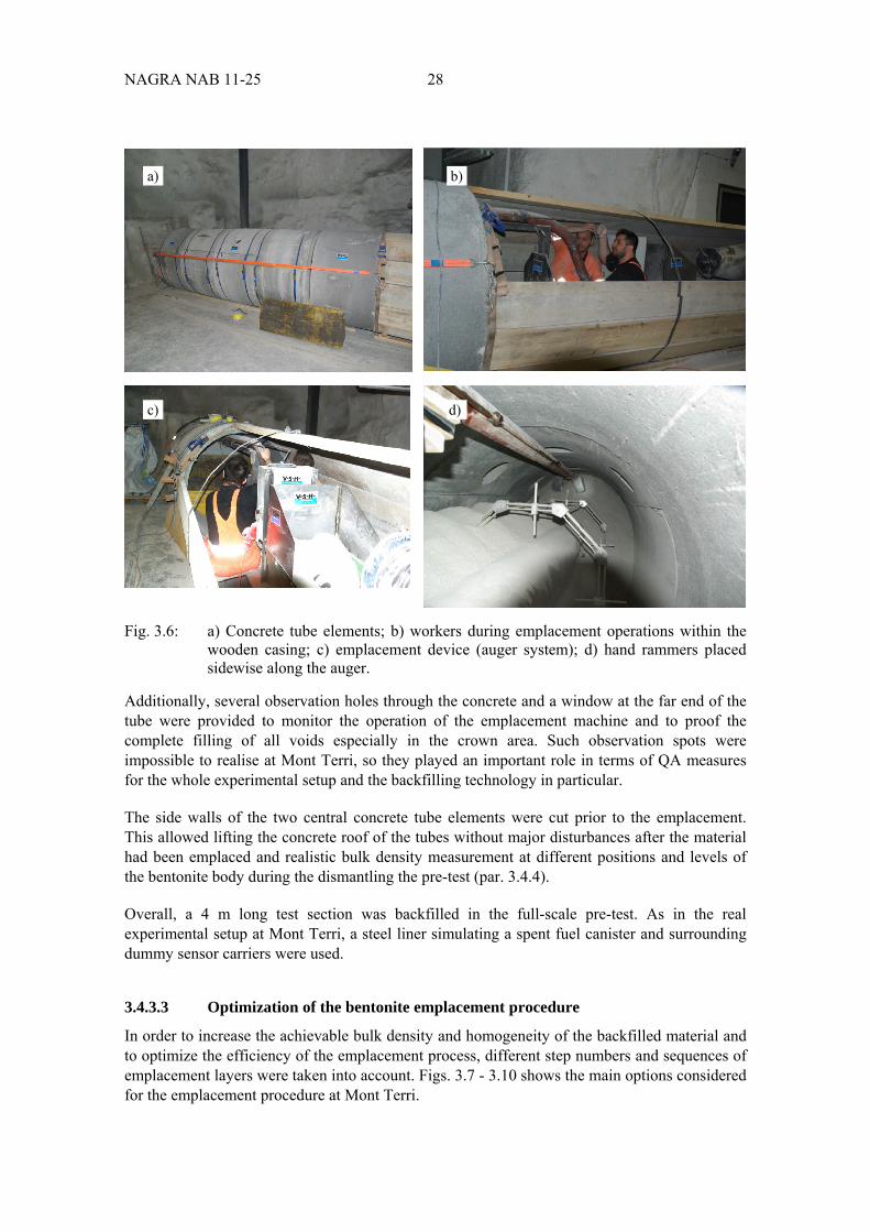
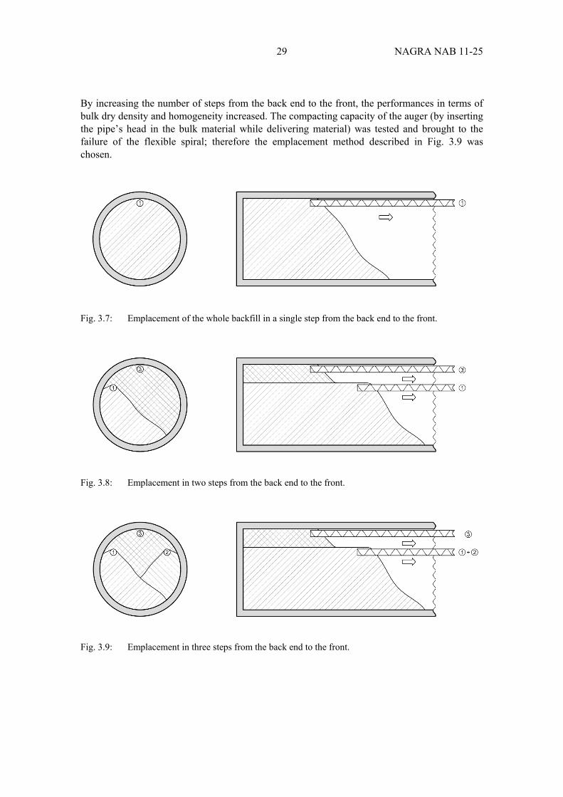
By increasing the number of steps from the back end to the front, the performances in terms of bulk dry density and homogeneity increased. The compacting capacity of the auger (by inserting the pipe’s head in the bulk material while delivering material) was tested and brought to the failure of the flexible spiral; therefore the emplacement method described in Fig. 3.9 was chosen.
Fig. 3.7: Emplacement of the whole backfill in a single step from the back end to the front.
Fig. 3.8: Emplacement in two steps from the back end to the front.
Fig. 3.9: Emplacement in three steps from the back end to the front.
NAGRA NAB 11-25 30
a)
b)
Fig. 3.10: Emplacement in three steps: a) two steps from front to back; b) one step from back end to the front.
3.4.3.4 Effect of compaction by a concrete vibrator
With regard to the two separately accessible material sections (where two of the concrete tubes were provided with observation holes and the upper part of which was pre-cut), the material in the central and upper part of one section was exposed to additional compaction by a concrete vibrator ("sampling interval 2") while the other parts were not ("sampling interval 1" and rest) (Fig. 3.12). The concrete vibrator was inserted into the backfill from the top at different filling stages (through the holes of the concrete tube) in order to basically test the effect of additional means of compaction.
3.4.4 Results and QA
During the dismantling of the pre-test the bulk density was measured with cutter cylinders at the different areas and levels. Moreover, the sensors' status was visually checked for damages and displacements (Fig. 3.11). Further observations were noted and qualitatively appraised. The values and positions of the measured bulk dry densities are shown in Fig. 3.12.
31 NAGRA NAB 11-25
Fig.3.11: a) – b) Test sections after dismantling the roof of the concrete tube; c) bentonite sampling with cutter cylinders; d) damaged sensor carrier element
Fig. 3.12: Dry densities of two backfilled granular bentonite sections. Left: emplacement by auger machine without further compaction. Right: emplacement by auger machine and material compacted with concrete vibrator.
During the dismantling progress, several observations were made that cannot be recorded quantitatively. These observations are summarized as follows:
a) b)
d)c)
NAGRA NAB 11-25 32
Local segregation of coarse grains observed while rolling down the filling slope, especially in the outer and bottom areas (Fig. 3.13)
Fig. 3.13: Segregation observed in a glass bowl placed onto the progressing slope of the filling material
Areas of segregation (small amount of fine grains) and low density found beside the bottom part of the steel liner and its bentonite block foundation.
Effect of vibrator compaction tentatively noticeable (Fig. 3.12, sampling interval 2), but very local.
In test interval 1 (no vibration compaction), tentatively higher densities were measured in the areas which were filled in two layers (left side) than in the areas filled in one layer (right side) (Fig. 3.12, sampling interval 1).
The target dry density was not reached in areas where flow shadows had been observed or significant segregation had taken place. Besides a correspondent general qualitative impression, this was also quantitatively recorded in the lower right parts where only a single backfilling layer was applied (Fig. 3.12).
Taking the undisturbed samples with cutter cylinders, different forces were needed for pressing them into the bulk material, corresponding to the local bulk density. In this regard, (modified) cone penetration tests could give additional results, e.g. in future QA programmes.
During bentonite emplacement some sensor carriers were displaced for 3 to 10 mm due to the bulk pressure of the bentonite granulate.
One part of a sensor dummy was broken (split), probably caused by hitting it with the auger or one of the hand rammers (Fig. 3.11 - d).
In terms of working conditions, dust formation was bearable when using breathing masks. Additional ventilation further improved the situation in the pre-test model.
3.4.5 Conclusions / Lessons learned
Based on the results of the pre-tests it was agreed, that the target dry density of 1.45 g/cm3 could better be reached by emplacing the bentonite material in three layers (left, right, middle / top) than in a single step.
Although certain effects on the material bulk texture could be observed locally using a concrete vibrator, no extra compaction was necessary to reach the target dry density.
Pushing the bentonite material with the auger caused blockage and damage to the flexible spiral.

33 NAGRA NAB 11-25
Longitudinal movement of the heavy emplacement machine with the 4.3 m long auger in the very restricted space between sensor carriers and tunnel wall was considered dangerous, especially if the railway system was uneven. The emplacement device should be able to move smoothly, the auger pipe had to be fixed firmly and stiffly.
Additionally, it was shown that the sensor carriers had to be stabilized horizontally to avoid displacement while filling in the bulk material.
Due to the observations during the pre-tests some adjustments of the emplacement and transport system had to be done. The auger pipe was equipped with a straining system to stabilise it horizontally and to make it better adjustable. The auger carrier had to be reinforced to make the system vertically stiffer and more stable. Additionally, some iron sheets were added to the system to reduce the dust pollution while transferring the bentonite from the truck agitator to the storage container of the emplacement machine.
The pre-tests gave an impression of the very restricted space in the real tunnel. Some difficulties with the emplacement equipment could be overcome in advance of its deployment at Mont Terri. Mechanical adjustment and fine tuning could be done under semi in situ circumstances with the benefit of the workshop infrastructure under laboratory conditions at Hagerbach Test Gallery.
3.5 Materials of the plugs
Three plugs are constructed in the HE-E experiment: 1) plug #1, bottom end of the experiment; 2) plug #2, separates the granular bentonite from the sand/bentonite section; 3) plug #3, isolates the experiment from the atmospheric conditions (more details are described in chapter 6, Figs. 6.2, 6.4 and 6.6). The construction sequence and utilized materials of the three plugs are summarized as follows:
Plug #1:
a. back end wall (cement bricks and mortar)
b. vapour barrier (aluminium foil)
c. thermal isolation (Rockwool)
d. dying end scaffolding wall for block (cement bricks and mortar)
e. block (concrete)
f. front scaffolding wall for block (cement bricks and mortar)
Plug #2:
a. back end wall for containment of bentonite material (cement bricks and mortar)
b. vapour barrier (aluminium foil)
c. thermal isolation (Rockwool)
d. vapour barrier (aluminium foil)

NAGRA NAB 11-25 34
e. front wall (cement bricks and mortar)
Plug #3:
a. back end wall for containment of sand/bentonite material (cement bricks and mortar)
b. thermal isolation (Rockwool)
c. vapour barrier (aluminium foil)
d. dying end scaffolding wall for block (cement bricks and mortar)
e. block (concrete)
f. front scaffolding wall for block (cement bricks and mortar)
3.5.1 Cement bricks
Utilized cement bricks are type Z 12, with dimensions: 25 x 12 x 13.5 cm used for common masonry works (Fig. 3.14) according to EN 998-2.
Fig. 3.14: Cement bricks type Z 12
3.5.2 Cement mortar
The mortar used to join the cement bricks was a ready-made dry mix to which water has been added. The cement mortar is mechanically classified as M15 according to EN 998-2 (Fig. 3.15).
Fig. 3.15: Cement mortar type M15 (Maxit 920)

35 NAGRA NAB 11-25
3.5.3 Concrete
A ready-made dry mix unreinforced concrete was poured into plug #1 and plug #3, mechanically classified as C30/37. The strength of the emplaced concrete, tested with three cubes according to the standard procedure EN 12390-3 (Appendix 2) showed up to 50.0 MPa.
3.5.4 Thermal isolation system and vapour barrier
As thermal isolation, Rockwool was selected because of its capacity to resist to temperatures higher than 1000°C. Rockwool is commercially available in cylinder forms (applied around the liner within the plugs) and in panel form (used to build the isolation walls of the plug) – Fig. 3.16. The thermal conductivity is 0.038 W/ (m K).
Fig. 3.16: Rockwoll (SPACEROCK RSK 830 and PARA) by FLUMROC AG.
The vapour barriers were made of two layers of aluminium foils (0.018 mm thickness each) with in between a glass fibre mesh (Fig. 3.17).
Fig. 3.17: Vapour barrier (TECHNONORM) by KORFF AG.
3.5.5 Quality Assurance
Materials are described by ad hoc-laboratory tests or certified by each producer in accordance to the relevant standards. All materials utilized for the construction of the HE-E experiment have well defined properties.

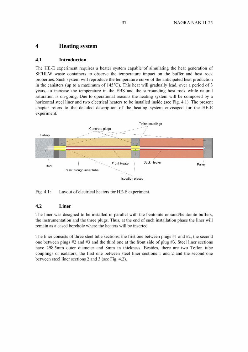
37 NAGRA NAB 11-25
4 Heating system
4.1 Introduction
The HE-E experiment requires a heater system capable of simulating the heat generation of SF/HLW waste containers to observe the temperature impact on the buffer and host rock properties. Such system will reproduce the temperature curve of the anticipated heat production in the canisters (up to a maximum of 145°C). This heat will gradually lead, over a period of 3 years, to increase the temperature in the EBS and the surrounding host rock while natural saturation is on-going. Due to operational reasons the heating system will be composed by a horizontal steel liner and two electrical heaters to be installed inside (see Fig. 4.1). The present chapter refers to the detailed description of the heating system envisaged for the HE-E experiment.
Fig. 4.1: Layout of electrical heaters for HE-E experiment.
4.2 Liner
The liner was designed to be installed in parallel with the bentonite or sand/bentonite buffers, the instrumentation and the three plugs. Thus, at the end of such installation phase the liner will remain as a cased borehole where the heaters will be inserted.
The liner consists of three steel tube sections: the first one between plugs #1 and #2, the second one between plugs #2 and #3 and the third one at the front side of plug #3. Steel liner sections have 298.5mm outer diameter and 8mm in thickness. Besides, there are two Teflon tube couplings or isolators, the first one between steel liner sections 1 and 2 and the second one between steel liner sections 2 and 3 (see Fig. 4.2).
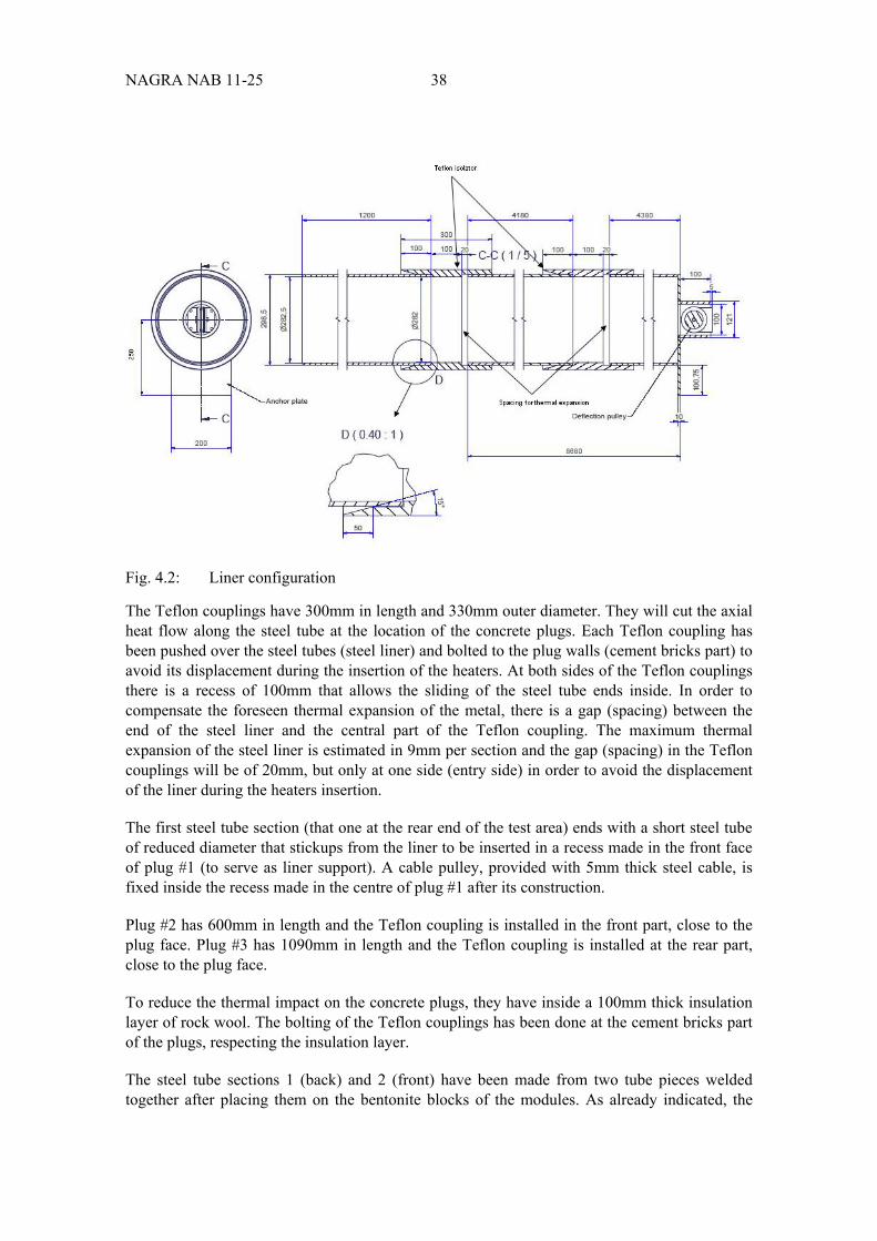
NAGRA NAB 11-25 38
Fig. 4.2: Liner configuration
The Teflon couplings have 300mm in length and 330mm outer diameter. They will cut the axial heat flow along the steel tube at the location of the concrete plugs. Each Teflon coupling has been pushed over the steel tubes (steel liner) and bolted to the plug walls (cement bricks part) to avoid its displacement during the insertion of the heaters. At both sides of the Teflon couplings there is a recess of 100mm that allows the sliding of the steel tube ends inside. In order to compensate the foreseen thermal expansion of the metal, there is a gap (spacing) between the end of the steel liner and the central part of the Teflon coupling. The maximum thermal expansion of the steel liner is estimated in 9mm per section and the gap (spacing) in the Teflon couplings will be of 20mm, but only at one side (entry side) in order to avoid the displacement of the liner during the heaters insertion.
The first steel tube section (that one at the rear end of the test area) ends with a short steel tube of reduced diameter that stickups from the liner to be inserted in a recess made in the front face of plug #1 (to serve as liner support). A cable pulley, provided with 5mm thick steel cable, is fixed inside the recess made in the centre of plug #1 after its construction.
Plug #2 has 600mm in length and the Teflon coupling is installed in the front part, close to the plug face. Plug #3 has 1090mm in length and the Teflon coupling is installed at the rear part, close to the plug face.
To reduce the thermal impact on the concrete plugs, they have inside a 100mm thick insulation layer of rock wool. The bolting of the Teflon couplings has been done at the cement bricks part of the plugs, respecting the insulation layer.
The steel tube sections 1 (back) and 2 (front) have been made from two tube pieces welded together after placing them on the bentonite blocks of the modules. As already indicated, the
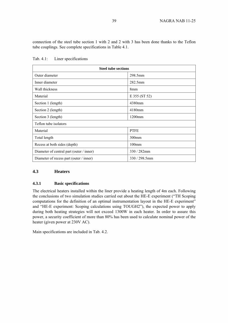
39 NAGRA NAB 11-25
connection of the steel tube section 1 with 2 and 2 with 3 has been done thanks to the Teflon tube couplings. See complete specifications in Table 4.1.
Tab. 4.1: Liner specifications
Steel tube sections
Outer diameter 298.5mm
Inner diameter 282.5mm
Wall thickness 8mm
Material E 355 (ST 52)
Section 1 (length) 4380mm
Section 2 (length) 4180mm
Section 3 (length) 1200mm
Teflon tube isolators
Material PTFE
Total length 300mm
Recess at both sides (depth) 100mm
Diameter of central part (outer / inner) 330 / 282mm
Diameter of recess part (outer / inner) 330 / 298.5mm
4.3 Heaters
4.3.1 Basic specifications
The electrical heaters installed within the liner provide a heating length of 4m each. Following the conclusions of two simulation studies carried out about the HE-E experiment (“TH Scoping computations for the definition of an optimal instrumentation layout in the HE-E experiment” and “HE-E experiment: Scoping calculations using TOUGH2”), the expected power to apply during both heating strategies will not exceed 1300W in each heater. In order to assure this power, a security coefficient of more than 80% has been used to calculate nominal power of the heater (given power at 230V AC).
Main specifications are included in Tab. 4.2.
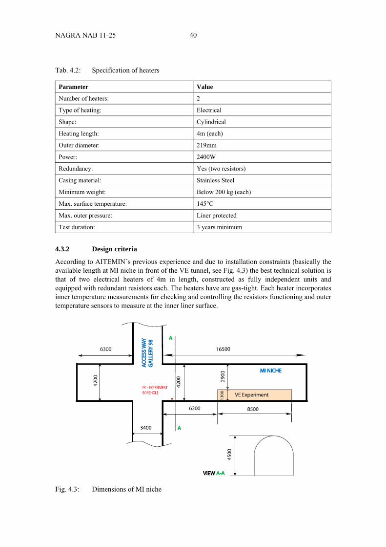
NAGRA NAB 11-25 40
Tab. 4.2: Specification of heaters
Parameter Value
Number of heaters: 2
Type of heating: Electrical
Shape: Cylindrical
Heating length: 4m (each)
Outer diameter: 219mm
Power: 2400W
Redundancy: Yes (two resistors)
Casing material: Stainless Steel
Minimum weight: Below 200 kg (each)
Max. surface temperature: 145°C
Max. outer pressure: Liner protected
Test duration: 3 years minimum
4.3.2 Design criteria
According to AITEMIN´s previous experience and due to installation constraints (basically the available length at MI niche in front of the VE tunnel, see Fig. 4.3) the best technical solution is that of two electrical heaters of 4m in length, constructed as fully independent units and equipped with redundant resistors each. The heaters have are gas-tight. Each heater incorporates inner temperature measurements for checking and controlling the resistors functioning and outer temperature sensors to measure at the inner liner surface.
Fig. 4.3: Dimensions of MI niche
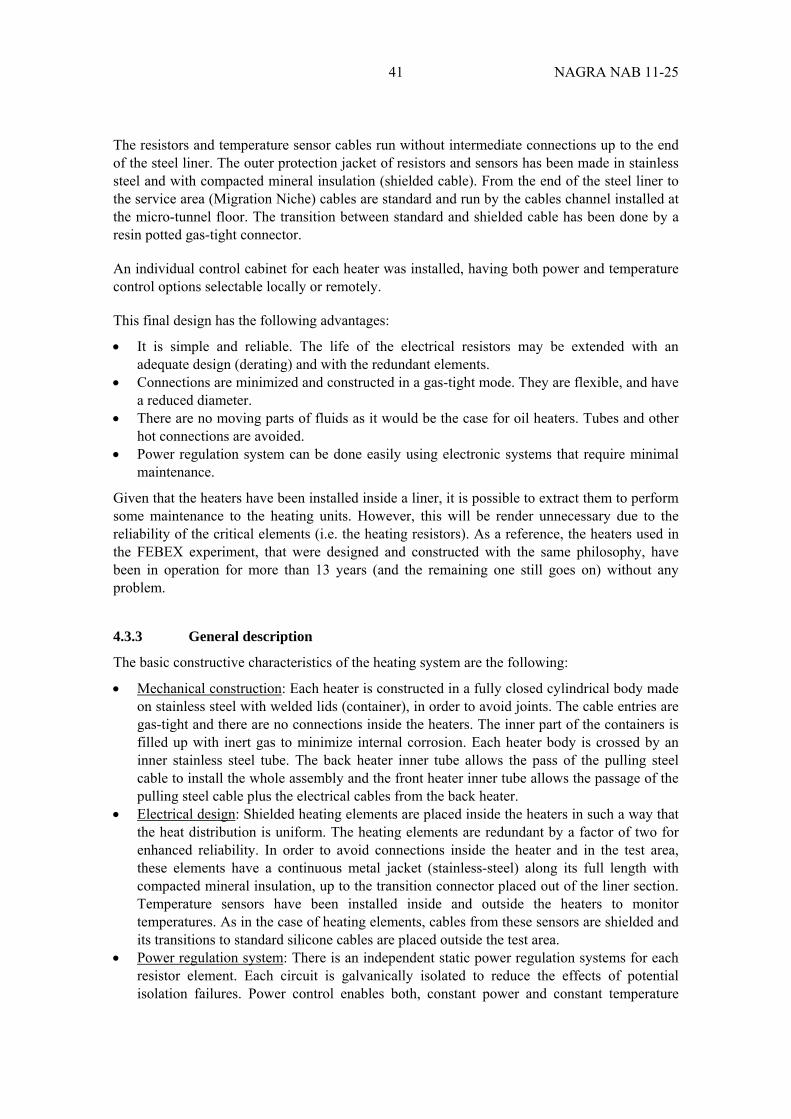
41 NAGRA NAB 11-25
The resistors and temperature sensor cables run without intermediate connections up to the end of the steel liner. The outer protection jacket of resistors and sensors has been made in stainless steel and with compacted mineral insulation (shielded cable). From the end of the steel liner to the service area (Migration Niche) cables are standard and run by the cables channel installed at the micro-tunnel floor. The transition between standard and shielded cable has been done by a resin potted gas-tight connector.
An individual control cabinet for each heater was installed, having both power and temperature control options selectable locally or remotely.
This final design has the following advantages:
It is simple and reliable. The life of the electrical resistors may be extended with an adequate design (derating) and with the redundant elements.
Connections are minimized and constructed in a gas-tight mode. They are flexible, and have a reduced diameter.
There are no moving parts of fluids as it would be the case for oil heaters. Tubes and other hot connections are avoided.
Power regulation system can be done easily using electronic systems that require minimal maintenance.
Given that the heaters have been installed inside a liner, it is possible to extract them to perform some maintenance to the heating units. However, this will be render unnecessary due to the reliability of the critical elements (i.e. the heating resistors). As a reference, the heaters used in the FEBEX experiment, that were designed and constructed with the same philosophy, have been in operation for more than 13 years (and the remaining one still goes on) without any problem.
4.3.3 General description
The basic constructive characteristics of the heating system are the following:
Mechanical construction: Each heater is constructed in a fully closed cylindrical body made on stainless steel with welded lids (container), in order to avoid joints. The cable entries are gas-tight and there are no connections inside the heaters. The inner part of the containers is filled up with inert gas to minimize internal corrosion. Each heater body is crossed by an inner stainless steel tube. The back heater inner tube allows the pass of the pulling steel cable to install the whole assembly and the front heater inner tube allows the passage of the pulling steel cable plus the electrical cables from the back heater.
Electrical design: Shielded heating elements are placed inside the heaters in such a way that the heat distribution is uniform. The heating elements are redundant by a factor of two for enhanced reliability. In order to avoid connections inside the heater and in the test area, these elements have a continuous metal jacket (stainless-steel) along its full length with compacted mineral insulation, up to the transition connector placed out of the liner section. Temperature sensors have been installed inside and outside the heaters to monitor temperatures. As in the case of heating elements, cables from these sensors are shielded and its transitions to standard silicone cables are placed outside the test area.
Power regulation system: There is an independent static power regulation systems for each resistor element. Each circuit is galvanically isolated to reduce the effects of potential isolation failures. Power control enables both, constant power and constant temperature
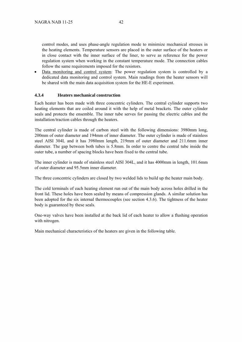
NAGRA NAB 11-25 42
control modes, and uses phase-angle regulation mode to minimize mechanical stresses in the heating elements. Temperature sensors are placed in the outer surface of the heaters or in close contact with the inner surface of the liner, to serve as reference for the power regulation system when working in the constant temperature mode. The connection cables follow the same requirements imposed for the resistors.
Data monitoring and control system: The power regulation system is controlled by a dedicated data monitoring and control system. Main readings from the heater sensors will be shared with the main data acquisition system for the HE-E experiment.
4.3.4 Heaters mechanical construction
Each heater has been made with three concentric cylinders. The central cylinder supports two heating elements that are coiled around it with the help of metal brackets. The outer cylinder seals and protects the ensemble. The inner tube serves for passing the electric cables and the installation/traction cables through the heaters.
The central cylinder is made of carbon steel with the following dimensions: 3980mm long, 200mm of outer diameter and 194mm of inner diameter. The outer cylinder is made of stainless steel AISI 304L and it has 3980mm length, 219mm of outer diameter and 211.6mm inner diameter. The gap between both tubes is 5.8mm. In order to centre the central tube inside the outer tube, a number of spacing blocks have been fixed to the central tube.
The inner cylinder is made of stainless steel AISI 304L, and it has 4000mm in length, 101.6mm of outer diameter and 95.5mm inner diameter.
The three concentric cylinders are closed by two welded lids to build up the heater main body.
The cold terminals of each heating element run out of the main body across holes drilled in the front lid. These holes have been sealed by means of compression glands. A similar solution has been adopted for the six internal thermocouples (see section 4.3.6). The tightness of the heater body is guaranteed by these seals.
One-way valves have been installed at the back lid of each heater to allow a flushing operation with nitrogen.
Main mechanical characteristics of the heaters are given in the following table.
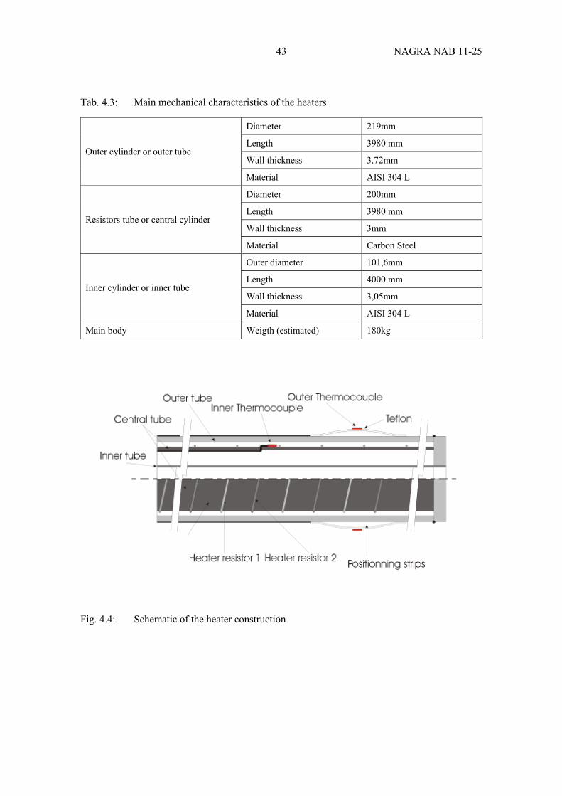
43 NAGRA NAB 11-25
Tab. 4.3: Main mechanical characteristics of the heaters
Diameter 219mm
Length 3980 mm
Wall thickness 3.72mm Outer cylinder or outer tube
Material AISI 304 L
Diameter 200mm
Length 3980 mm
Wall thickness 3mm Resistors tube or central cylinder
Material Carbon Steel
Outer diameter 101,6mm
Length 4000 mm
Wall thickness 3,05mm Inner cylinder or inner tube
Material AISI 304 L
Main body Weigth (estimated) 180kg
Fig. 4.4: Schematic of the heater construction
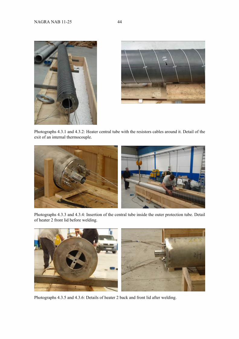
NAGRA NAB 11-25 44
Photographs 4.3.1 and 4.3.2: Heater central tube with the resistors cables around it. Detail of the exit of an internal thermocouple.
Photographs 4.3.3 and 4.3.4: Insertion of the central tube inside the outer protection tube. Detail of heater 2 front lid before welding.
Photographs 4.3.5 and 4.3.6: Details of heater 2 back and front lid after welding.
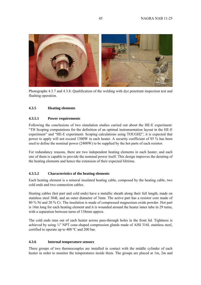
45 NAGRA NAB 11-25
Photographs 4.3.7 and 4.3.8: Qualification of the welding with dye penetrant inspection test and flushing operation.
4.3.5 Heating elements
4.3.5.1 Power requirements
Following the conclusions of two simulation studies carried out about the HE-E experiment: “TH Scoping computations for the definition of an optimal instrumentation layout in the HE-E experiment” and “HE-E experiment: Scoping calculations using TOUGH2”, it is expected that power to apply will not exceed 1300W in each heater. A security coefficient of 85 % has been used to define the nominal power (2400W) to be supplied by the hot parts of each resistor.
For redundancy reasons, there are two independent heating elements in each heater, and each one of them is capable to provide the nominal power itself. This design improves the derating of the heating elements and hence the extension of their expected lifetime.
4.3.5.2 Characteristics of the heating elements
Each heating element is a mineral insulated heating cable, composed by the heating cable, two cold ends and two connection cables.
Heating cables (hot part and cold ends) have a metallic sheath along their full length, made on stainless steel 304L and an outer diameter of 3mm. The active part has a resistor core made of 80 % Ni and 20 % Cr. The insulation is made of compressed magnesium oxide powder. Hot part is 16m long for each heating element and it is wounded around the heater inner tube in 29 turns, with a separation between turns of 138mm approx.
The cold ends runs out of each heater across pass-through holes in the front lid. Tightness is achieved by using ¼” NPT cone-shaped compression glands made of AISI 316L stainless steel, certified to operate up to 400 ºC and 200 bar.
4.3.6 Internal temperature sensors
Three groups of two thermocouples are installed in contact with the middle cylinder of each heater in order to monitor the temperatures inside them. The groups are placed at 1m, 2m and
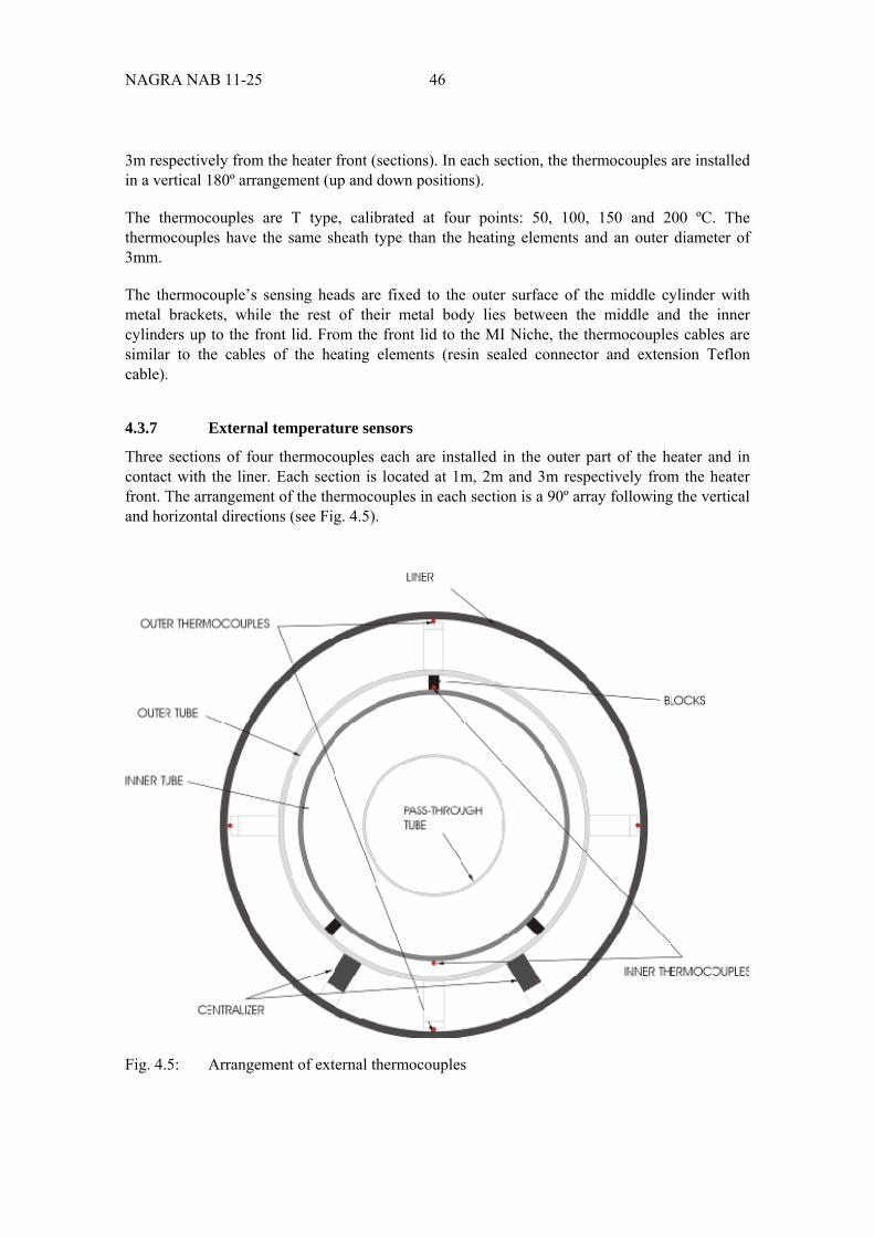
NAGRA NAB 11-25 46
3m respectively from the heater front (sections). In each section, the thermocouples are installed in a vertical 180º arrangement (up and down positions).
The thermocouples are T type, calibrated at four points: 50, 100, 150 and 200 ºC. The thermocouples have the same sheath type than the heating elements and an outer diameter of 3mm.
The thermocouple’s sensing heads are fixed to the outer surface of the middle cylinder with metal brackets, while the rest of their metal body lies between the middle and the inner cylinders up to the front lid. From the front lid to the MI Niche, the thermocouples cables are similar to the cables of the heating elements (resin sealed connector and extension Teflon cable).
4.3.7 External temperature sensors
Three sections of four thermocouples each are installed in the outer part of the heater and in contact with the liner. Each section is located at 1m, 2m and 3m respectively from the heater front. The arrangement of the thermocouples in each section is a 90º array following the vertical and horizontal directions (see Fig. 4.5).
Fig. 4.5: Arrangement of external thermocouples
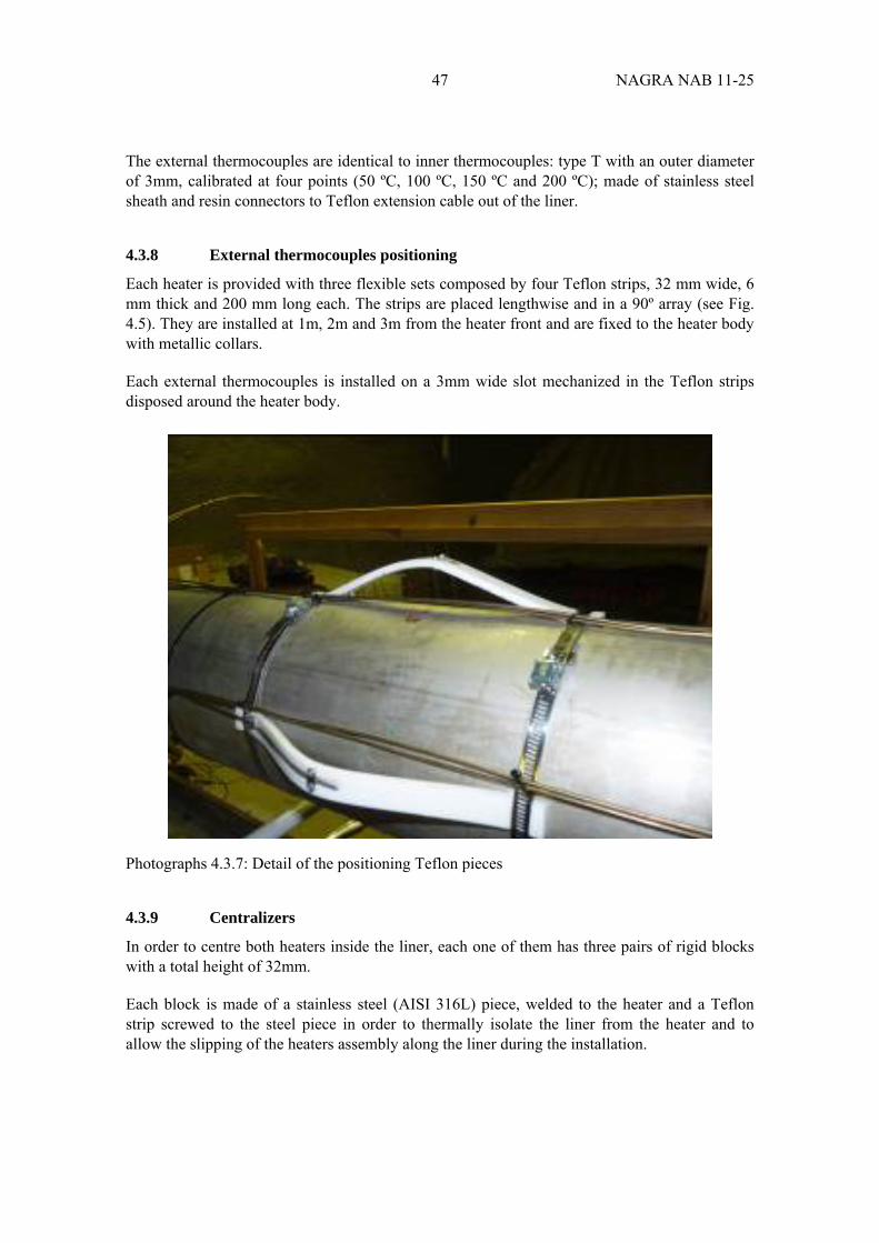
47 NAGRA NAB 11-25
The external thermocouples are identical to inner thermocouples: type T with an outer diameter of 3mm, calibrated at four points (50 ºC, 100 ºC, 150 ºC and 200 ºC); made of stainless steel sheath and resin connectors to Teflon extension cable out of the liner.
4.3.8 External thermocouples positioning
Each heater is provided with three flexible sets composed by four Teflon strips, 32 mm wide, 6 mm thick and 200 mm long each. The strips are placed lengthwise and in a 90º array (see Fig. 4.5). They are installed at 1m, 2m and 3m from the heater front and are fixed to the heater body with metallic collars.
Each external thermocouples is installed on a 3mm wide slot mechanized in the Teflon strips disposed around the heater body.
Photographs 4.3.7: Detail of the positioning Teflon pieces
4.3.9 Centralizers
In order to centre both heaters inside the liner, each one of them has three pairs of rigid blocks with a total height of 32mm.
Each block is made of a stainless steel (AISI 316L) piece, welded to the heater and a Teflon strip screwed to the steel piece in order to thermally isolate the liner from the heater and to allow the slipping of the heaters assembly along the liner during the installation.
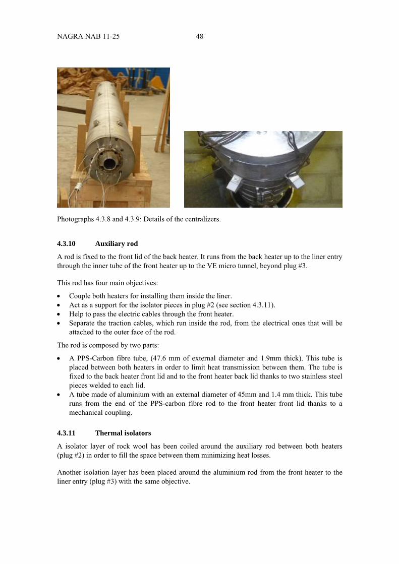
NAGRA NAB 11-25 48
Photographs 4.3.8 and 4.3.9: Details of the centralizers.
4.3.10 Auxiliary rod
A rod is fixed to the front lid of the back heater. It runs from the back heater up to the liner entry through the inner tube of the front heater up to the VE micro tunnel, beyond plug #3.
This rod has four main objectives:
Couple both heaters for installing them inside the liner. Act as a support for the isolator pieces in plug #2 (see section 4.3.11). Help to pass the electric cables through the front heater. Separate the traction cables, which run inside the rod, from the electrical ones that will be
attached to the outer face of the rod.
The rod is composed by two parts:
A PPS-Carbon fibre tube, (47.6 mm of external diameter and 1.9mm thick). This tube is placed between both heaters in order to limit heat transmission between them. The tube is fixed to the back heater front lid and to the front heater back lid thanks to two stainless steel pieces welded to each lid.
A tube made of aluminium with an external diameter of 45mm and 1.4 mm thick. This tube runs from the end of the PPS-carbon fibre rod to the front heater front lid thanks to a mechanical coupling.
4.3.11 Thermal isolators
A isolator layer of rock wool has been coiled around the auxiliary rod between both heaters (plug #2) in order to fill the space between them minimizing heat losses.
Another isolation layer has been placed around the aluminium rod from the front heater to the liner entry (plug #3) with the same objective.
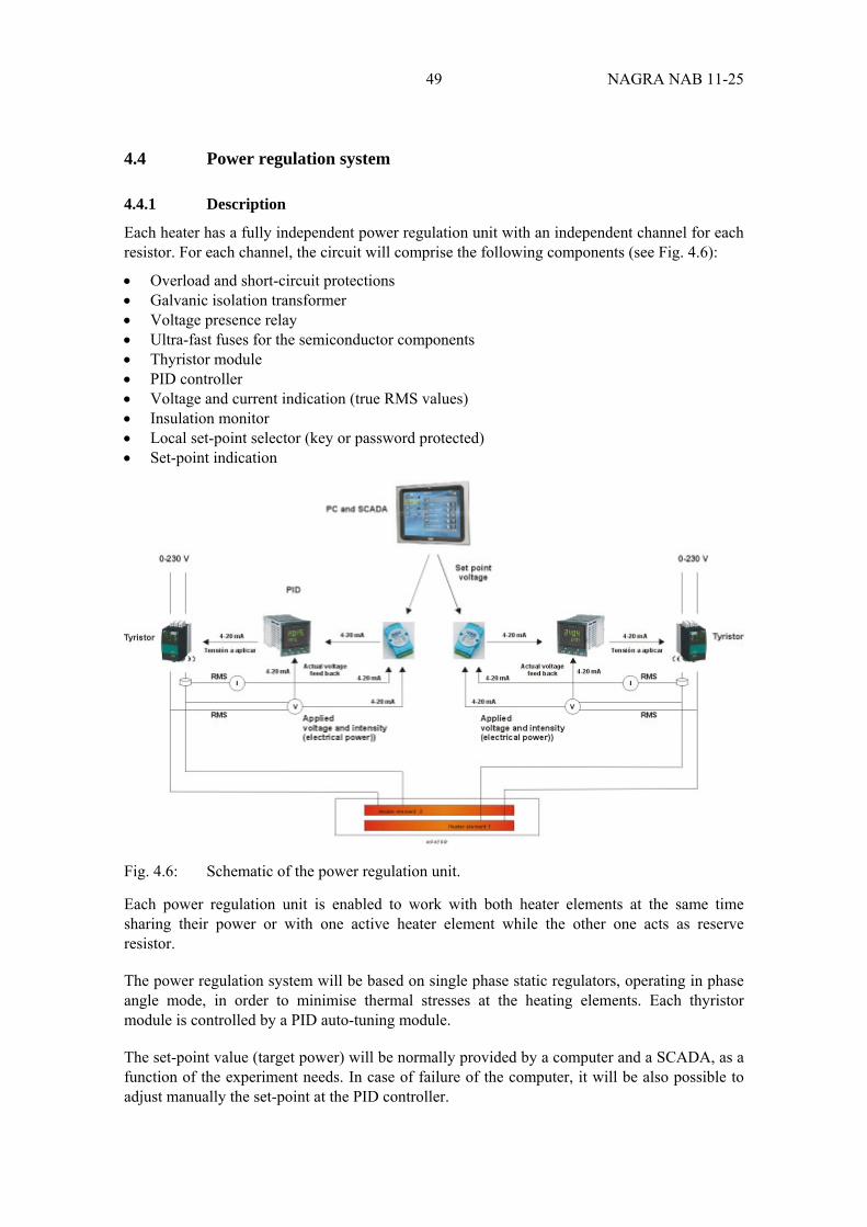
49 NAGRA NAB 11-25
4.4 Power regulation system
4.4.1 Description
Each heater has a fully independent power regulation unit with an independent channel for each resistor. For each channel, the circuit will comprise the following components (see Fig. 4.6):
Overload and short-circuit protections Galvanic isolation transformer Voltage presence relay Ultra-fast fuses for the semiconductor components Thyristor module PID controller Voltage and current indication (true RMS values) Insulation monitor Local set-point selector (key or password protected) Set-point indication
Fig. 4.6: Schematic of the power regulation unit.
Each power regulation unit is enabled to work with both heater elements at the same time sharing their power or with one active heater element while the other one acts as reserve resistor.
The power regulation system will be based on single phase static regulators, operating in phase angle mode, in order to minimise thermal stresses at the heating elements. Each thyristor module is controlled by a PID auto-tuning module.
The set-point value (target power) will be normally provided by a computer and a SCADA, as a function of the experiment needs. In case of failure of the computer, it will be also possible to adjust manually the set-point at the PID controller.

NAGRA NAB 11-25 50
There are two modes of operation:
Constant power: The PID controller will receive an external set-point in power or voltage and a feedback of the actual power or voltage applied to the heater. Then the PID will adjust the power or voltage in the heating element by regulating the voltage applied to the element by the thyristor, so to keep it at the set-point value.
Constant temperature. In this case, the SCADA will use as regulation temperature the highest of the outer temperature recorded. Depending on this temperature the SCADA will give the set point to the PID.
The actual voltage applied and current consumption of each heating element (true RMS values), as well as the isolation to earth, will be measured by means of electrical signal converters. These converters will provide a 4-20mA output that will be used for local indication and also as an input to the data acquisition and control system.
4.4.2 Specifications
The specifications for the main components of the power regulation units are as follows:
Thyristors. Monophase, electric supply of 230V, inputs 4-20mA, regulation phase angle, external fuses.
PID. Input 4-20mA, output 4-20mA, electric supply 230V, auto-tuning and manual mode. Voltage measure instrumentation. Effective voltage transformer, input 230V, output
4-20mA, electric supply 230V. Current measure instrumentation. Current transformer, electric supply 230V. Isolation measure instrumentation. Isolation detector, electric supply 230V.
4.5 Monitoring and control system
For safety and redundancy reasons, each power regulation unit will be provided with its own monitoring and control system.
4.5.1 Functions and structure
The functions of the control system are the following:
a. To acquire, store and display the information provided by the instruments installed in the heater.
b. To generate the commands required at each moment for the power regulation, upon the basis of the experiment control strategy.
c. To transfer information to the general data acquisition system.
d. To enable remote access to the system via network for remote monitoring and maintenance.
The control system will be composed by the following main components:
Signal conditioning and data acquisition unit Host Computer (industrial PC) Uninterrupted Power Supply unit

51 NAGRA NAB 11-25
4.5.2 Signal conditioning and data acquisition unit
A standard data conditioning/acquisition unit will receive the signals from all the instruments installed in the heater. The signals connected to this unit are:
Current, voltage, isolation power on/off for each heating element Heaters temperatures (inner and outer)
These signals are transmitted to the host computer via a serial link, and stored internally for redundant data storage, enabling the recovery of the information in case of experiment main computer failure.
4.5.3 Host Computer
A host computer is envisaged for controlling each heater. The host computer is a standard industrial computer (rugged PC) located into a protection cabinet. The PC reads the data from the signal conditioning and data acquisition unit, and processes, displays, and stores these data in an internal data base. The computer also generates the power set point for the heater power regulation units, as a function of the programmed control strategy, which could be configured and adapted to each situation either locally or remotely. Finally, main data are transmitted to the general Data Acquisition System of the HE-E experiment by means of a serial link.
A general purpose SCADA firmware will is used to perform the following main functions:
Continuous data acquisition from the signal conditioning and data logging Data conversion into physical units Adaptation of conversion functions Data presentation (text and graphical) Data storage into internal data base Heaters set point calculation and writing to the power regulation units Display of heaters status and alarms generation
The data base at the PC contains the values of the measurements (one every ten minutes). However, this rate can be modified if necessary at some specific moments (for example during the start-up period).
Remote access to the host computer is done via network using an internet connection and a well proven dedicated communications firmware. This enables to perform the heater control remote supervision, to dump stored data, and to modify the power control strategy, if necessary. Access (by keyboard or remotely) to the computer is restricted by means of a specific entry password.
4.5.4 Uninterrupted Power Supply
The PC, the signal conditioning and data acquisition unit, the power controllers and the auxiliary power of the power regulation cabinets are backed-up with an Uninterrupted Power Supply (UPS) In case of mains network shutdown, the UPS guarantees the power supply to these devices for a 10-15 minutes time period. Heating elements are not backed-up by the UPS.
The UPS will work in the “on-line” mode (output voltage is separated from input and battery-buffered), minimising disturbances from mains network.

NAGRA NAB 11-25 52
4.5.5 Specifications
The specifications for the main components of the data acquisition unit are as follows:
Rugged PC and LCD screen, equipped with USB, Ethernet and RS232 ports. Thermocouple acquisition data module. Thermocouples measures are read with an eight
input channels and eight digital outputs module. Main characteristics are: Precision (AI/TC): ±0.1 %. Input impedance > 10MΩ. Thermocouples type: J, K, T, E, R, S and B. Resolution (AI/TC): 16 bit / ±0.1 % FSR. Sampling speed: 10 par second. Ethernet 10/100 bas T. Protocol Modbus/TCp, TCP/IP, UDP and http. Electric supply: 10-30V DC. Operation temperature: -10 ºC to +70 ºC. Storage temperature: -10 ºC to +80 ºC. Power consumption: 2W at 24V DC.
Signal 4-20mA acquisition data module. Voltage and intensity lectures are made via an acquisition universal module with six/two analogical input/output channels and two/two digital input/output channels. Main characteristics are: Sampling ratio: 10 per second. Ethernet 10/100 bas T. Protocol Modbus/TCp, TCP/IP, UDP and http. Electric supply: 10-30V DC. Operation temperature: -10 ºC to +50 ºC. Storage temperature: -20 ºC to +80 ºC. Power consumption: 4W at 24V DC.
Analogical inputs: Input impedance: 20MΩ. Input: 0-10V, 4-20mA et 0-20mA. Precision: ±0.1 %. Resolution: 16 bit / ±0.1 % FSR.
Analogical outputs: Output: 0-10V, 4-20mA et 0-20mA. Precision: ±0.1 %. Resolution: 12 bit / ±0.1 % FSR.
Ethernet hub. In order to send all the different information to the PC a five ports Ethernet module is being used. Main characteristics are: Ethernet 10/100 bas TX. Transmission length: more than 100m. Transmission speed: more than 100 MBps. Protocol: Modbus/TCP, TCP/IP, UDP and http. Voltage: 10-30V DC. Operation temperature: -10 ºC to +70 ºC. Storage temperature: -20 ºC to +80 ºC. Power consumption: 3W at 24V DC.

53 NAGRA NAB 11-25
4.6 Quality Control
Close quality control has been applied to the following components:
Material composition and dimensions of the metallic components of the heaters Resistors of the heaters Temperature sensors Measuring devices of the power regulation system PIDs Thyristors Cable glands for the heaters Centralisers Computer and UPS of the monitoring and control system SCADA software
Quality control has been applied to the following operations:
Resistors and inner thermocouples installation and operational checking Welding of the heaters and checking of final tightness Inner flushing of the heaters Operational checking of centralisers with the outer thermocouples Power regulation assembly and functioning in both modes Monitoring and control system assembly and functioning Full operational checking at AITEMIN facilities before delivery Installation operation at Mont Terri Final checks and controls at Mont Terri after installation

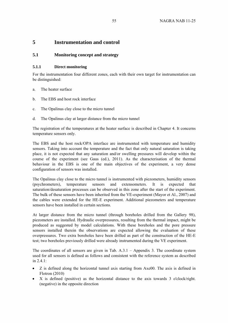
55 NAGRA NAB 11-25
5 Instrumentation and control
5.1 Monitoring concept and strategy
5.1.1 Direct monitoring
For the instrumentation four different zones, each with their own target for instrumentation can be distinguished:
a. The heater surface
b. The EBS and host rock interface
c. The Opalinus clay close to the micro tunnel
d. The Opalinus clay at larger distance from the micro tunnel
The registration of the temperatures at the heater surface is described in Chapter 4. It concerns temperature sensors only.
The EBS and the host rock/OPA interface are instrumented with temperature and humidity sensors. Taking into account the temperature and the fact that only natural saturation is taking place, it is not expected that any saturation and/or swelling pressures will develop within the course of the experiment (see Gaus (ed.), 2011). As the characterisation of the thermal behaviour in the EBS is one of the main objectives of the experiment, a very dense configuration of sensors was installed.
The Opalinus clay close to the micro tunnel is instrumented with piezometers, humidity sensors (psychrometers), temperature sensors and extensometers. It is expected that saturation/desaturation processes can be observed in this zone after the start of the experiment. The bulk of these sensors have been inherited from the VE-experiment (Mayor et Al., 2007) and the cables were extended for the HE-E experiment. Additional piezometers and temperature sensors have been installed in certain sections.
At larger distance from the micro tunnel (through boreholes drilled from the Gallery 98), piezometers are installed. Hydraulic overpressures, resulting from the thermal impact, might be produced as suggested by model calculations. With these boreholes and the pore pressure sensors installed therein the observations are expected allowing the evaluation of these overpressures. Two extra boreholes have been drilled as part of the construction of the HE-E test; two boreholes previously drilled were already instrumented during the VE experiment.
The coordinates of all sensors are given in Tab. A.3.1 – Appendix 3. The coordinate system used for all sensors is defined as follows and consistent with the reference system as described in 2.4.1:
Z is defined along the horizontal tunnel axis starting from Axe00. The axis is defined in Flotron (2010)
X is defined (positive) as the horizontal distance to the axis towards 3 o'clock/right. (negative) in the opposite direction

NAGRA NAB 11-25 56
Y is defined (positive) as the vertical distance to the axis towards 12 o'clock/upwards. (negative) in the opposite direction.
The coordinate system is a mathematical (right-hand) system.
The coordinates from BVE boreholes (Mont Terri Technical Note 2003-11) are moved to fit with the recent situation. The offset estimated with respect to the sections is:
Z: + 0.228m; X: + 0.994m; Y: - 0.040m
5.1.2 Indirect monitoring
Next to these direct measurements described in the previous paragraph, instruments for indirect measurements have been emplaced:
Network for geo-electric sensors
An electrode array was installed in four 1 metre deep boreholes and on the tunnel surface in a section through the micro tunnel in 2003 (Mayor et al., 2007). The equipment was renovated in 2010. Evaluation of the geoelectric four-point measurements leads to a two-dimensional resistivity distribution that is expected to be close to the true resistivity field. Through calibration based on laboratory tests information on the water saturation can be obtained.
Seismic array
A seismic array consisting of five piezoelectric transducers which serve as emitters and ten transducers which serve as receivers were installed in three 1 metre deep boreholes in a section of the micro tunnel. The seismic transmission experiment aims at characterising changes in the Opalinus Clay and EBS properties caused by the heating.
5.2 Temperature and humidity sensors in the EBS and the EBS/host rock interface.
The temperature and the relative air humidity are the key monitoring parameters for the EBS and the interface.
5.2.1 Types and locations
A total of 18 humidity/temperature sensors are emplaced at the tunnel wall and an additional 60 humidity / temperature sensors are emplaced within the sand/bentonite or bentonite section. The position of the sensors in a cross-section through the micro tunnel is shown in Fig. 5.1.
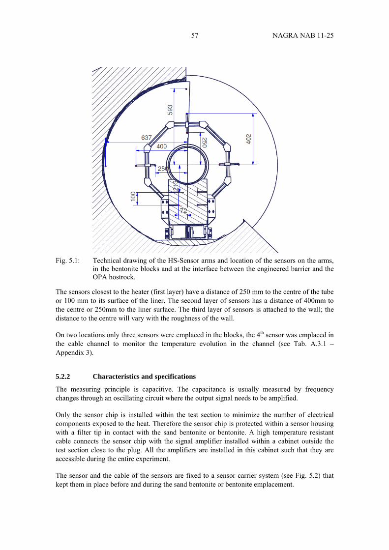
57 NAGRA NAB 11-25
Fig. 5.1: Technical drawing of the HS-Sensor arms and location of the sensors on the arms, in the bentonite blocks and at the interface between the engineered barrier and the OPA hostrock.
The sensors closest to the heater (first layer) have a distance of 250 mm to the centre of the tube or 100 mm to its surface of the liner. The second layer of sensors has a distance of 400mm to the centre or 250mm to the liner surface. The third layer of sensors is attached to the wall; the distance to the centre will vary with the roughness of the wall.
On two locations only three sensors were emplaced in the blocks, the 4th sensor was emplaced in the cable channel to monitor the temperature evolution in the channel (see Tab. A.3.1 – Appendix 3).
5.2.2 Characteristics and specifications
The measuring principle is capacitive. The capacitance is usually measured by frequency changes through an oscillating circuit where the output signal needs to be amplified.
Only the sensor chip is installed within the test section to minimize the number of electrical components exposed to the heat. Therefore the sensor chip is protected within a sensor housing with a filter tip in contact with the sand bentonite or bentonite. A high temperature resistant cable connects the sensor chip with the signal amplifier installed within a cabinet outside the test section close to the plug. All the amplifiers are installed in this cabinet such that they are accessible during the entire experiment.
The sensor and the cable of the sensors are fixed to a sensor carrier system (see Fig. 5.2) that kept them in place before and during the sand bentonite or bentonite emplacement.
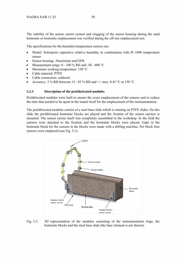
NAGRA NAB 11-25 58
The stability of the sensor carrier system and clogging of the sensor housing during the sand bentonite or bentonite emplacement was verified during the off-site emplacement test.
The specifications for the humidity/temperature sensors are:
Model: Solexperts capacitive relative humidity in combination with Pt 1000 temperature sensor
Sensor housing: Aluminium and GFK Measurement range: 0 - 100 % RH and -50 - 400 °C Maximum working temperature: 150 °C Cable material: PTFE Cable connection: soldered Accuracy: 3 % RH between 15 - 85 % RH and +/- max. 0.45 °C at 150 °C
5.2.3 Description of the prefabricated modules
Prefabricated modules were built to ensure the exact emplacement of the sensors and to reduce the time that needed to be spent in the tunnel itself for the emplacement of the instrumentation.
The prefabricated modules consist of a steel base slide which is running on PTFE slides. On this slide the prefabricated bentonite blocks are placed and the fixation of the sensor carriers is mounted. The sensor carrier itself was completely assembled in the workshop. In the field the carriers were attached to the fixation and the bentonite blocks were placed. Gaps in the bentonite block for the sensors in the blocks were made with a drilling machine. Per block four sensors were emplaced (see Fig. 5.1).
Fig. 5.2: 3D representation of the modules consisting of the instrumentation rings, the bentonite blocks and the steel base slide (the liner element is not shown).
59 NAGRA NAB 11-25
For each section of the experiment the modules were connected on the platform outside the micro tunnel and then towed into the micro tunnel. The technical drawing for the connected modules forming one section of the experiment is given in Fig. 5.3.
Fig. 5.3: Technical drawing of the 3 connected modules for one of the sections and the location of the instrumentation arms with respect to the plugs.
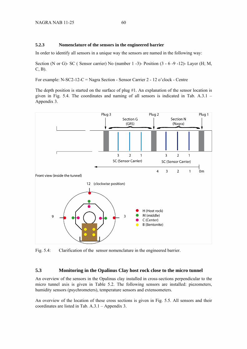
NAGRA NAB 11-25 60
5.2.3 Nomenclature of the sensors in the engineered barrier
In order to identify all sensors in a unique way the sensors are named in the following way:
Section (N or G)- SC ( Sensor carrier) No (number 1 -3)- Position (3 - 6 -9 -12)- Layer (H; M, C, B).
For example: N-SC2-12-C = Nagra Section - Sensor Carrier 2 - 12 o’clock - Centre
The depth position is started on the surface of plug #1. An explanation of the sensor location is given in Fig. 5.4. The coordinates and naming of all sensors is indicated in Tab. A.3.1 – Appendix 3.
Fig. 5.4: Clarification of the sensor nomenclature in the engineered barrier.
5.3 Monitoring in the Opalinus Clay host rock close to the micro tunnel
An overview of the sensors in the Opalinus clay installed in cross-sections perpendicular to the micro tunnel axis is given in Table 5.2. The following sensors are installed: piezometers, humidity sensors (psychrometers), temperature sensors and extensometers.
An overview of the location of these cross sections is given in Fig. 5.5. All sensors and their coordinates are listed in Tab. A.3.1 – Appendix 3.
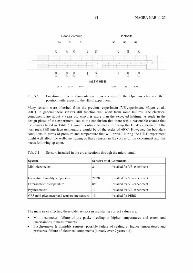
61 NAGRA NAB 11-25
Fig. 5.5: Location of the instrumentation cross sections in the Opalinus clay and their position with respect to the HE-E experiment
Many sensors were inherited from the previous experiment (VE-experiment, Mayor et al., 2007). In general these sensors still function well apart from some failures. The electrical components are about 9 years old which is more than the expected lifetime. A study in the design phase of the experiment lead to the conclusion that there was a reasonable chance that the sensors listed in Table 5.1 would continue to measure during the HE-E experiment if the host rock/EBS interface temperature would be of the order of 60°C. However, the boundary conditions in terms of pressure and temperature that will prevail during the HE-E experiment might well affect the well-functioning of these sensors in the course of the experiment and this needs following up upon.
Tab. 5.1: Sensors installed in the cross-sections through the microtunnel.
System Sensors total Comments
Mini-piezometers 24 Installed for VE-experiment
Capacitive humidity/temperature 20/20 Installed for VE-experiment
Extensometer / temperature 8/8 Installed for VE-experiment
Psychrometers 17 Installed for VE-experiment
GRS mini-piezometer and temperature sensors 10 Installed for PEBS
The main risks affecting these older sensors in registering correct values are:
Mini-piezometer: failure of the packer sealing at higher temperatures and errors and uncertainties in measurements
Psychrometer & humidity sensors: possible failure of sealing at higher temperatures and pressures, failure of electrical components (already over 9 years old).
Sand/Bentonite Bentonite
N1N2N3G1G2G3
32.78 33.78 34.7830.1829.1828.18
[m] TM HE-E
SA
127
.98
SB
128
.98
SA
229
.63
SD
13
0.88
SA
33
1.48
SD
23
3.33
SB
23
3.98
SA
43
4.98

NAGRA NAB 11-25 62
5.3.1 Detailed description of instrumentation inherited from the VE-experiment
Mini Piezometers (MPPs)
The system layout of the Solexperts Mini-Piezometer System is shown in a generalized 3D drawing (Fig. 5.6).
The specifications of the mini-piezometer systems are:
Borehole diameter: 30 mm
Maximum borehole depth: 2 m
Quantity: 24 mini piezometers systems – 2 cross-sections SA2 and SA4 with 8 mini piezometers and 2 cross-sections SA1 and SA3 with 4 mini-piezometers.
Packer system description:
Filter chamber (interval) with two flow lines - mechanical packer – resin section
Control unit description:
a. Pressure line: 3-way valve, manometer and pressure transducer
b. Flow line: 2-way valve
c. One multi-control unit for 8 mini-piezometers, Total of 4 units
d. One electrical connection box for each unit (water proof, but not water tight)
e. (upward systems with resin packer)
System dimensions:
Interval length: 15 to 30 cm
Packer length: 10 cm
Material specifications:
Filter: 60 microns mesh sintered polyethylene filters (porosity: ~ 30 %, OD = 29 mm)
Packer: Synthetic rubber and stainless steel
Flow lines:
a. Within interval: Stainless steel (OD 4 mm, ID 2 mm).
b. From interval to control unit: Polyamide lines (OD 6mm, ID 2mm)
Resin sealing section: Epoxy resin
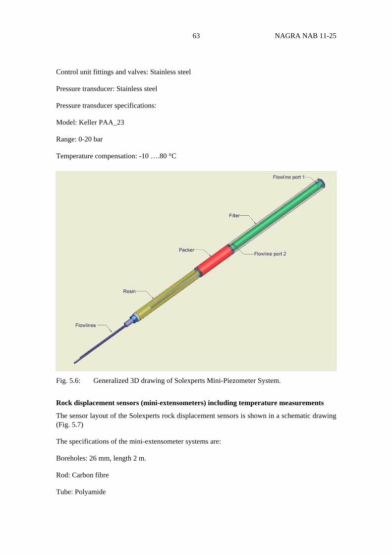
63 NAGRA NAB 11-25
Control unit fittings and valves: Stainless steel
Pressure transducer: Stainless steel
Pressure transducer specifications:
Model: Keller PAA_23
Range: 0-20 bar
Temperature compensation: -10 ….80 °C
Fig. 5.6: Generalized 3D drawing of Solexperts Mini-Piezometer System.
Rock displacement sensors (mini-extensometers) including temperature measurements
The sensor layout of the Solexperts rock displacement sensors is shown in a schematic drawing (Fig. 5.7)
The specifications of the mini-extensometer systems are:
Boreholes: 26 mm, length 2 m.
Rod: Carbon fibre
Tube: Polyamide
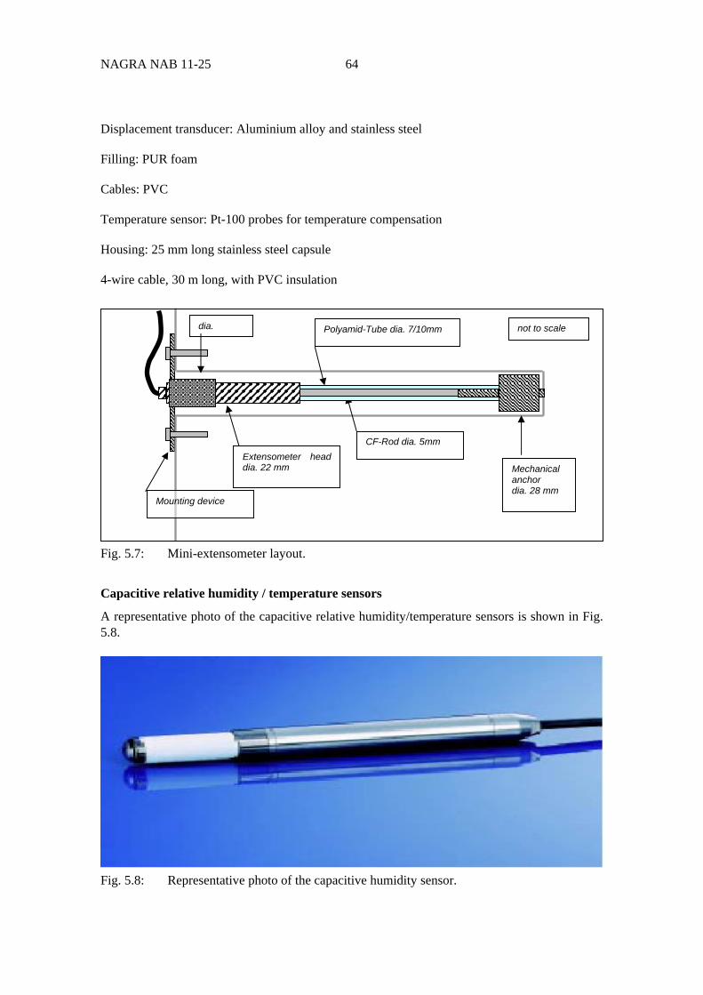
NAGRA NAB 11-25 64
Displacement transducer: Aluminium alloy and stainless steel
Filling: PUR foam
Cables: PVC
Temperature sensor: Pt-100 probes for temperature compensation
Housing: 25 mm long stainless steel capsule
4-wire cable, 30 m long, with PVC insulation
Fig. 5.7: Mini-extensometer layout.
Capacitive relative humidity / temperature sensors
A representative photo of the capacitive relative humidity/temperature sensors is shown in Fig. 5.8.
Fig. 5.8: Representative photo of the capacitive humidity sensor.
dia.
CF-Rod dia. 5mm
Polyamid-Tube dia. 7/10mm
Mechanical anchor dia. 28 mm
Mounting device
Extensometer head dia. 22 mm
not to scale

65 NAGRA NAB 11-25
The 20 capacitive relative humidity/temperature sensors are placed in boreholes located in the two profiles SB1 and SB2. Section SB1 is equipped with 8 sensors, section SB2 with 12.
The specifications for the sensors are:
Boreholes: 26 mm, length up to 200 cm
Model: ROTRONIC Type S (I-2000) with Pt100 temperature sensor
Sensor: Stainless steel
Range: 0- 100 % RH
Temperature range: -40….180 °C
Cables: FEP
Cable connection: Epoxy sealed
Psychrometer type relative humidity sensors
The sensor layout of the psychrometer type relative humidity sensors is shown in a schematic drawing (Fig. 5.9). These sensors are placed in boreholes located in the two profiles SB1 and SB2 (Fig. 5.4). Both sections are equipped with 8 psychrometers each plus an additional surface sensor.
The specifications for the sensors are:
Boreholes: 26 mm, length up to 200 cm
Model: WESCOR type PST-55
Filter: Ceramic filter
Probe material: Teflon-vinyl
Range: 95 – 99.96 % RH
Temperature range: -200 ….350 °C
Cables: PVC
Cable connection: Epoxy sealed
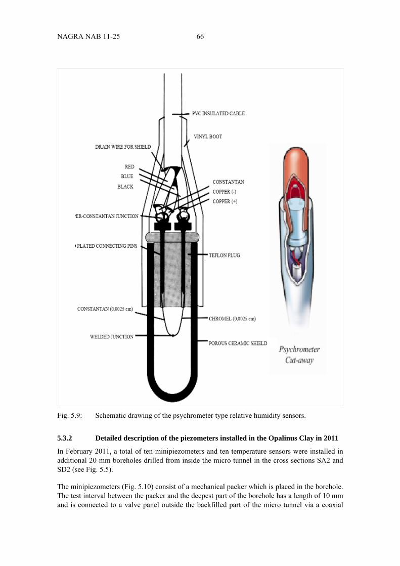
NAGRA NAB 11-25 66
Fig. 5.9: Schematic drawing of the psychrometer type relative humidity sensors.
5.3.2 Detailed description of the piezometers installed in the Opalinus Clay in 2011
In February 2011, a total of ten minipiezometers and ten temperature sensors were installed in additional 20-mm boreholes drilled from inside the micro tunnel in the cross sections SA2 and SD2 (see Fig. 5.5).
The minipiezometers (Fig. 5.10) consist of a mechanical packer which is placed in the borehole. The test interval between the packer and the deepest part of the borehole has a length of 10 mm and is connected to a valve panel outside the backfilled part of the micro tunnel via a coaxial
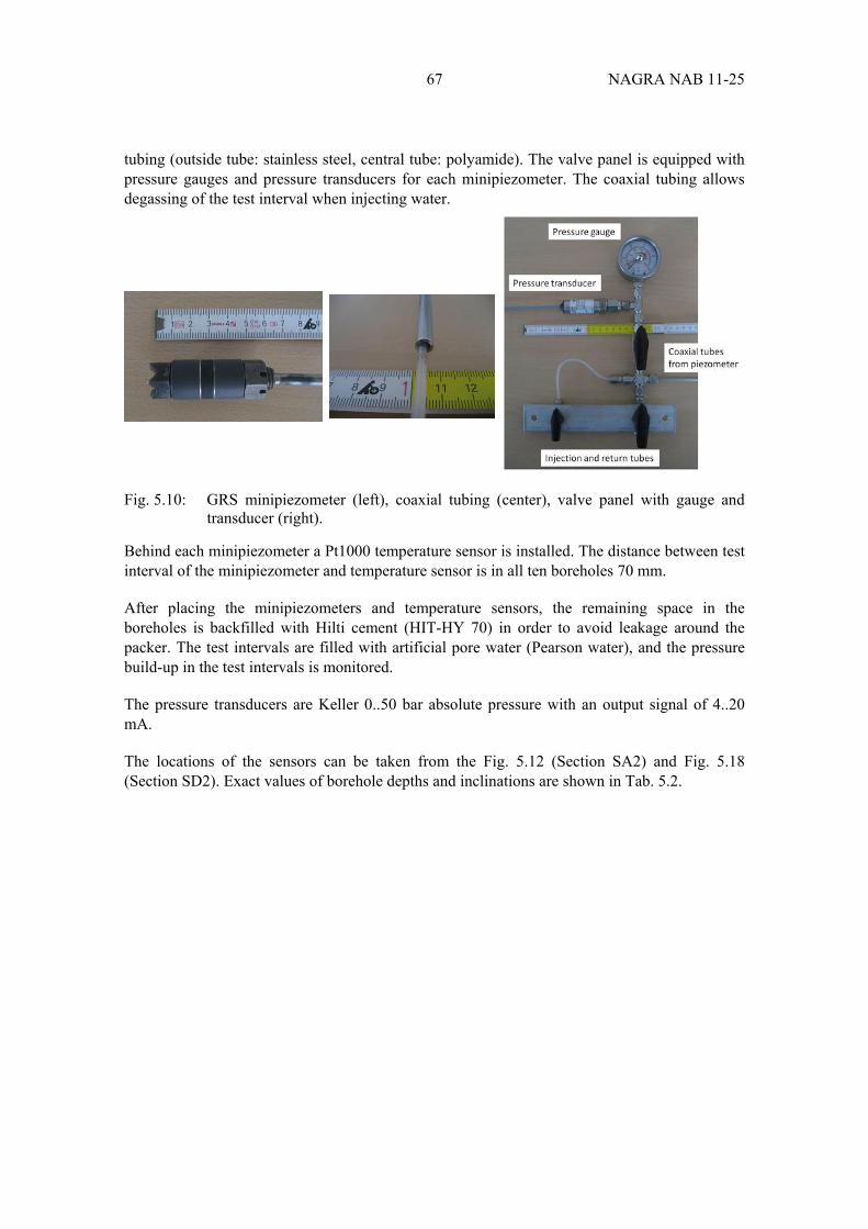
67 NAGRA NAB 11-25
tubing (outside tube: stainless steel, central tube: polyamide). The valve panel is equipped with pressure gauges and pressure transducers for each minipiezometer. The coaxial tubing allows degassing of the test interval when injecting water.
Fig. 5.10: GRS minipiezometer (left), coaxial tubing (center), valve panel with gauge and transducer (right).
Behind each minipiezometer a Pt1000 temperature sensor is installed. The distance between test interval of the minipiezometer and temperature sensor is in all ten boreholes 70 mm.
After placing the minipiezometers and temperature sensors, the remaining space in the boreholes is backfilled with Hilti cement (HIT-HY 70) in order to avoid leakage around the packer. The test intervals are filled with artificial pore water (Pearson water), and the pressure build-up in the test intervals is monitored.
The pressure transducers are Keller 0..50 bar absolute pressure with an output signal of 4..20 mA.
The locations of the sensors can be taken from the Fig. 5.12 (Section SA2) and Fig. 5.18 (Section SD2). Exact values of borehole depths and inclinations are shown in Tab. 5.2.
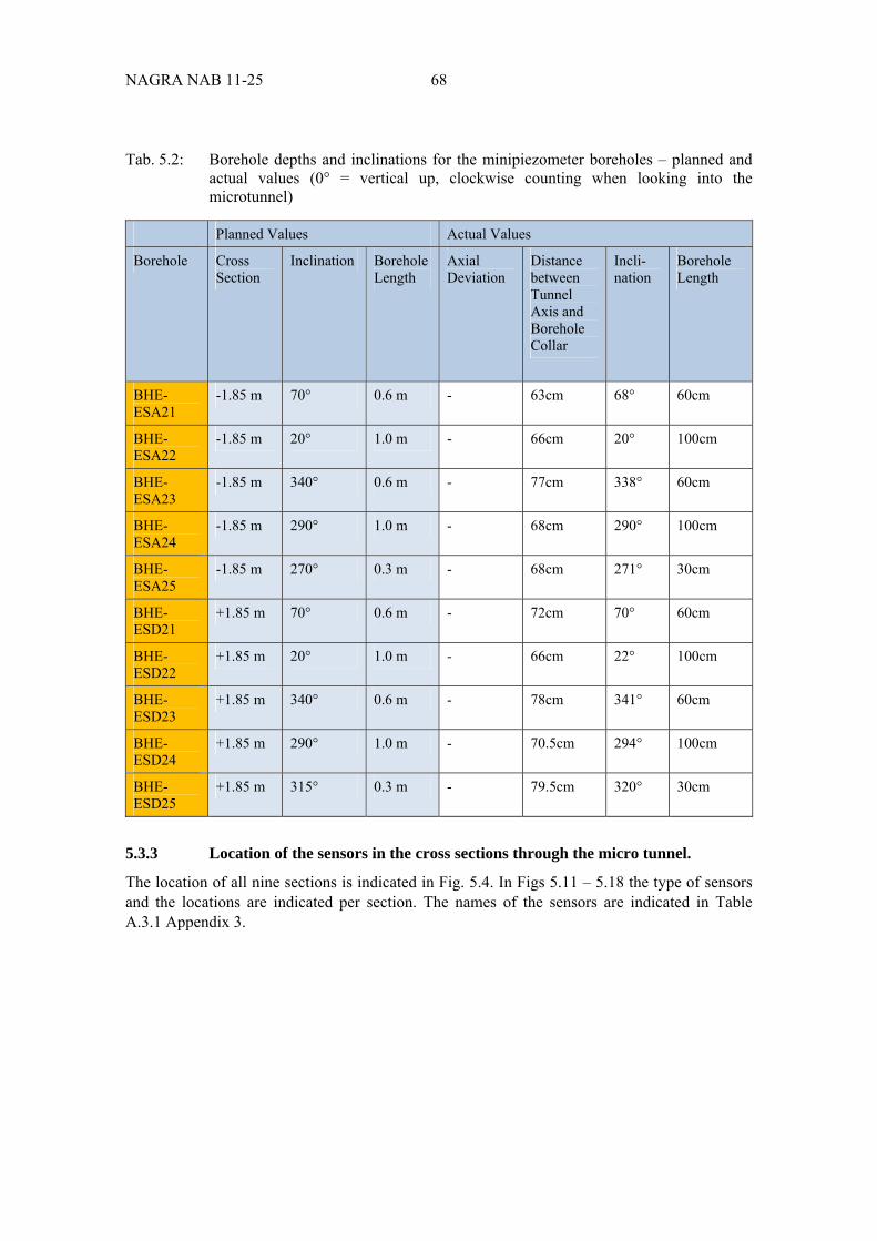
NAGRA NAB 11-25 68
Tab. 5.2: Borehole depths and inclinations for the minipiezometer boreholes – planned and actual values (0° = vertical up, clockwise counting when looking into the microtunnel)
Planned Values Actual Values
Borehole Cross Section
Inclination Borehole Length
Axial Deviation
Distance between Tunnel Axis and Borehole Collar
Incli-nation
Borehole Length
BHE-ESA21
-1.85 m 70° 0.6 m - 63cm 68° 60cm
BHE-ESA22
-1.85 m 20° 1.0 m - 66cm 20° 100cm
BHE-ESA23
-1.85 m 340° 0.6 m - 77cm 338° 60cm
BHE-ESA24
-1.85 m 290° 1.0 m - 68cm 290° 100cm
BHE-ESA25
-1.85 m 270° 0.3 m - 68cm 271° 30cm
BHE-ESD21
+1.85 m 70° 0.6 m - 72cm 70° 60cm
BHE-ESD22
+1.85 m 20° 1.0 m - 66cm 22° 100cm
BHE-ESD23
+1.85 m 340° 0.6 m - 78cm 341° 60cm
BHE-ESD24
+1.85 m 290° 1.0 m - 70.5cm 294° 100cm
BHE-ESD25
+1.85 m 315° 0.3 m - 79.5cm 320° 30cm
5.3.3 Location of the sensors in the cross sections through the micro tunnel.
The location of all nine sections is indicated in Fig. 5.4. In Figs 5.11 – 5.18 the type of sensors and the locations are indicated per section. The names of the sensors are indicated in Table A.3.1 Appendix 3.
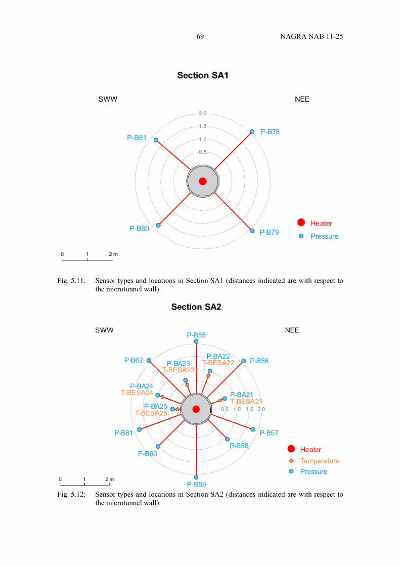
69 NAGRA NAB 11-25
Fig. 5.11: Sensor types and locations in Section SA1 (distances indicated are with respect to the microtunnel wall).
Fig. 5.12: Sensor types and locations in Section SA2 (distances indicated are with respect to the microtunnel wall).
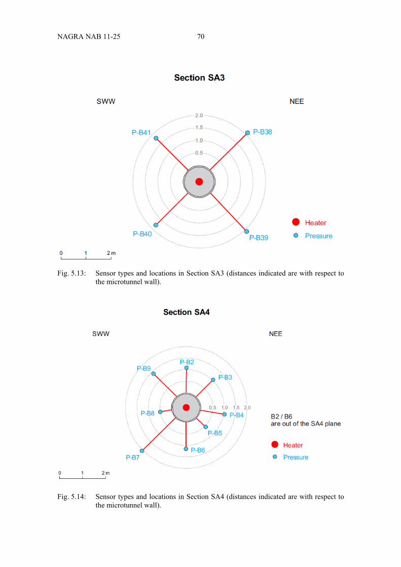
NAGRA NAB 11-25 70
Fig. 5.13: Sensor types and locations in Section SA3 (distances indicated are with respect to the microtunnel wall).
Fig. 5.14: Sensor types and locations in Section SA4 (distances indicated are with respect to the microtunnel wall).
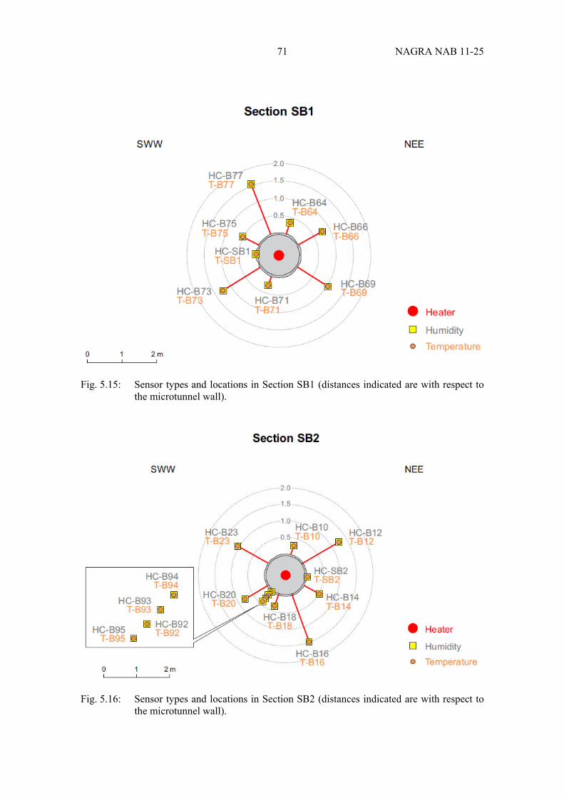
71 NAGRA NAB 11-25
Fig. 5.15: Sensor types and locations in Section SB1 (distances indicated are with respect to the microtunnel wall).
Fig. 5.16: Sensor types and locations in Section SB2 (distances indicated are with respect to the microtunnel wall).
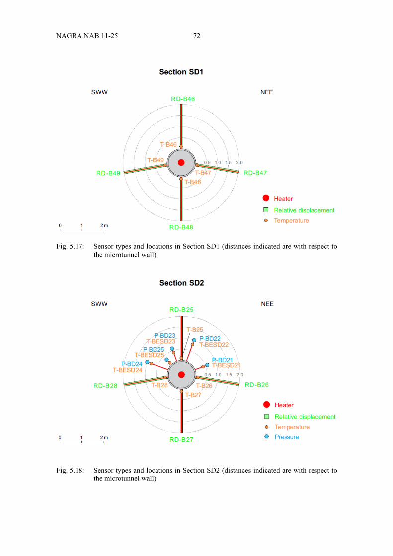
NAGRA NAB 11-25 72
Fig. 5.17: Sensor types and locations in Section SD1 (distances indicated are with respect to the microtunnel wall).
Fig. 5.18: Sensor types and locations in Section SD2 (distances indicated are with respect to the microtunnel wall).
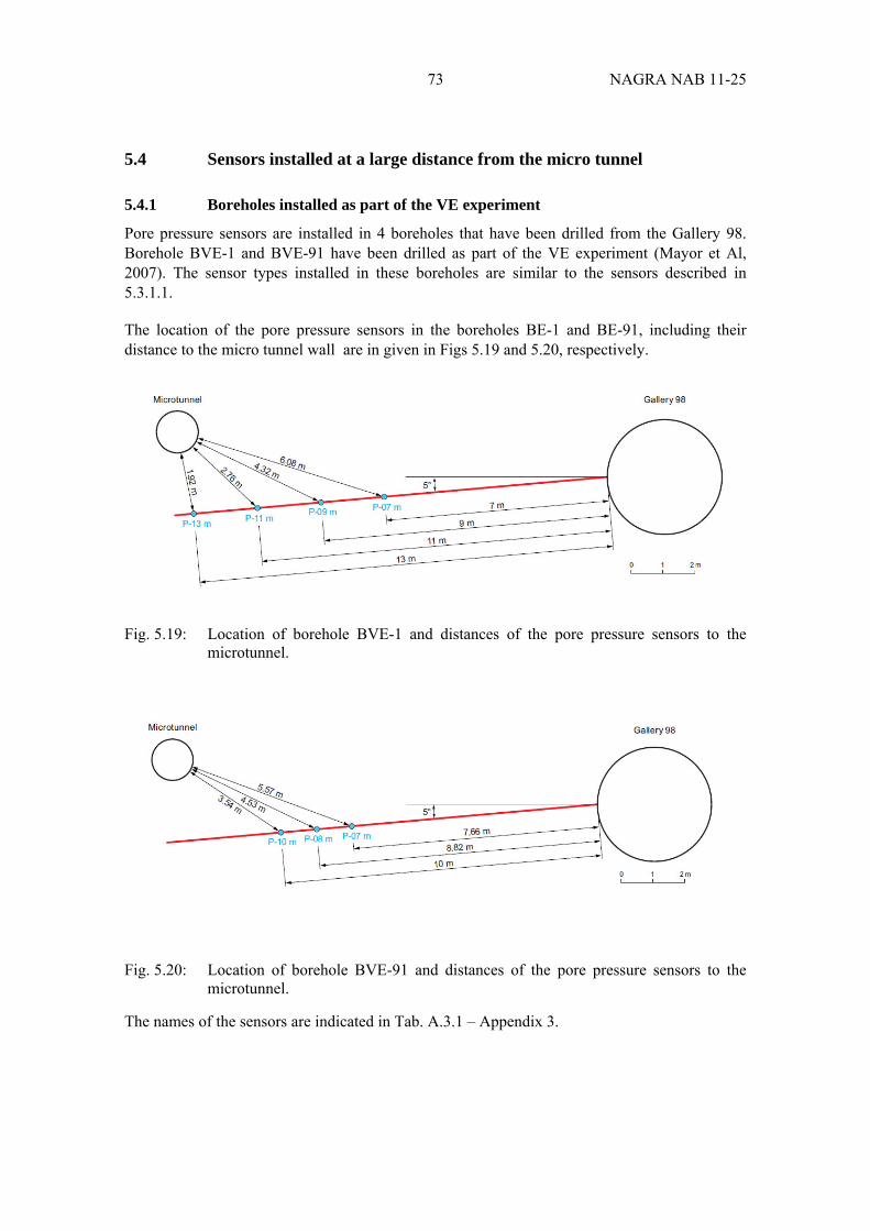
73 NAGRA NAB 11-25
5.4 Sensors installed at a large distance from the micro tunnel
5.4.1 Boreholes installed as part of the VE experiment
Pore pressure sensors are installed in 4 boreholes that have been drilled from the Gallery 98. Borehole BVE-1 and BVE-91 have been drilled as part of the VE experiment (Mayor et Al, 2007). The sensor types installed in these boreholes are similar to the sensors described in 5.3.1.1.
The location of the pore pressure sensors in the boreholes BE-1 and BE-91, including their distance to the micro tunnel wall are in given in Figs 5.19 and 5.20, respectively.
Fig. 5.19: Location of borehole BVE-1 and distances of the pore pressure sensors to the microtunnel.
Fig. 5.20: Location of borehole BVE-91 and distances of the pore pressure sensors to the microtunnel.
The names of the sensors are indicated in Tab. A.3.1 – Appendix 3.
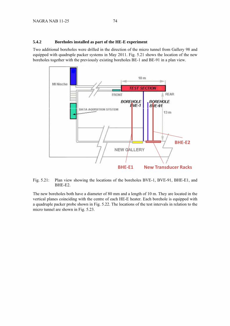
NAGRA NAB 11-25 74
5.4.2 Boreholes installed as part of the HE-E experiment
Two additional boreholes were drilled in the direction of the micro tunnel from Gallery 98 and equipped with quadruple packer systems in May 2011. Fig. 5.21 shows the location of the new boreholes together with the previously existing boreholes BE-1 and BE-91 in a plan view.
Fig. 5.21: Plan view showing the locations of the boreholes BVE-1, BVE-91, BHE-E1, and BHE-E2.
The new boreholes both have a diameter of 80 mm and a length of 10 m. They are located in the vertical planes coinciding with the centre of each HE-E heater. Each borehole is equipped with a quadruple packer probe shown in Fig. 5.22. The locations of the test intervals in relation to the micro tunnel are shown in Fig. 5.23.
BHE‐E1
BHE‐E2
New Transducer Racks
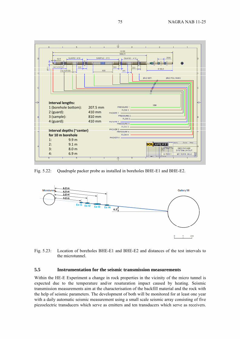
75 NAGRA NAB 11-25
Fig. 5.22: Quadruple packer probe as installed in boreholes BHE-E1 and BHE-E2.
Fig. 5.23: Location of boreholes BHE-E1 and BHE-E2 and distances of the test intervals to the microtunnel.
5.5 Instrumentation for the seismic transmission measurements
Within the HE-E Experiment a change in rock properties in the vicinity of the micro tunnel is expected due to the temperature and/or resaturation impact caused by heating. Seismic transmission measurements aim at the characterisation of the backfill material and the rock with the help of seismic parameters. The development of both will be monitored for at least one year with a daily automatic seismic measurement using a small scale seismic array consisting of five piezoelectric transducers which serve as emitters and ten transducers which serve as receivers.
Interval lengths:1 (borehole bottom): 207.5 mm2 (guard): 410 mm3 (sample): 810 mm4 (guard): 410 mm
Interval depths (~center)for 10 m borehole1: 9.9 m2: 9.1 m3: 8.0 m4: 6.9 m
6.2°Ex‐I4
3.0 m
3.8 m4.9 m6.0 m
Ex‐I1 Ex‐I2 Ex‐I3
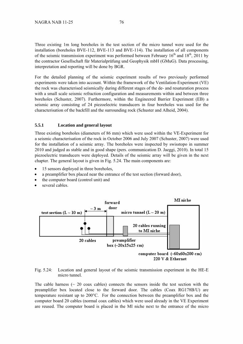
NAGRA NAB 11-25 76
Three existing 1m long boreholes in the test section of the micro tunnel were used for the installation (boreholes BVE-112, BVE-113 and BVE-114). The installation of all components of the seismic transmission experiment was performed between February 16th and 18th, 2011 by the contractor Gesellschaft für Materialprüfung und Geophysik mbH (GMuG). Data processing, interpretation and reporting will be done by BGR.
For the detailed planning of the seismic experiment results of two previously performed experiments were taken into account. Within the framework of the Ventilation-Experiment (VE) the rock was characterised seismically during different stages of the de- and resaturation process with a small scale seismic refraction configuration and measurements within and between three boreholes (Schuster, 2007). Furthermore, within the Engineered Barrier Experiment (EB) a seismic array consisting of 24 piezoelectric transducers in four boreholes was used for the characterisation of the backfill and the surrounding rock (Schuster and Alheid, 2004).
5.5.1 Location and general layout
Three existing boreholes (diameters of 86 mm) which were used within the VE-Experiment for a seismic characterisation of the rock in October 2006 and July 2007 (Schuster, 2007) were used for the installation of a seismic array. The boreholes were inspected by swisstopo in summer 2010 and judged as stable and in good shape (pers. communication D. Jaeggi, 2010). In total 15 piezoelectric transducers were deployed. Details of the seismic array will be given in the next chapter. The general layout is given in Fig. 5.24. The main components are:
15 sensors deployed in three boreholes, a preamplifier box placed near the entrance of the test section (forward door), the computer board (control unit) and several cables.
Fig. 5.24: Location and general layout of the seismic transmission experiment in the HE-E micro tunnel.
The cable harness (~ 20 coax cables) connects the sensors inside the test section with the preamplifier box located close to the forward door. The cables (Coax RG178B/U) are temperature resistant up to 200°C. For the connection between the preamplifier box and the computer board 20 cables (normal coax cables) which were used already in the VE Experiment are reused. The computer board is placed in the MI niche next to the entrance of the micro
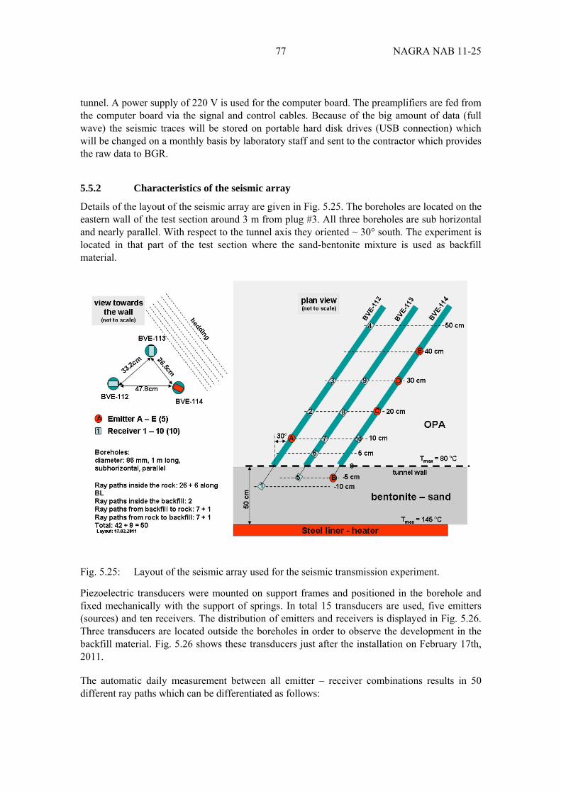
77 NAGRA NAB 11-25
tunnel. A power supply of 220 V is used for the computer board. The preamplifiers are fed from the computer board via the signal and control cables. Because of the big amount of data (full wave) the seismic traces will be stored on portable hard disk drives (USB connection) which will be changed on a monthly basis by laboratory staff and sent to the contractor which provides the raw data to BGR.
5.5.2 Characteristics of the seismic array
Details of the layout of the seismic array are given in Fig. 5.25. The boreholes are located on the eastern wall of the test section around 3 m from plug #3. All three boreholes are sub horizontal and nearly parallel. With respect to the tunnel axis they oriented ~ 30° south. The experiment is located in that part of the test section where the sand-bentonite mixture is used as backfill material.
Fig. 5.25: Layout of the seismic array used for the seismic transmission experiment.
Piezoelectric transducers were mounted on support frames and positioned in the borehole and fixed mechanically with the support of springs. In total 15 transducers are used, five emitters (sources) and ten receivers. The distribution of emitters and receivers is displayed in Fig. 5.26. Three transducers are located outside the boreholes in order to observe the development in the backfill material. Fig. 5.26 shows these transducers just after the installation on February 17th, 2011.
The automatic daily measurement between all emitter – receiver combinations results in 50 different ray paths which can be differentiated as follows:
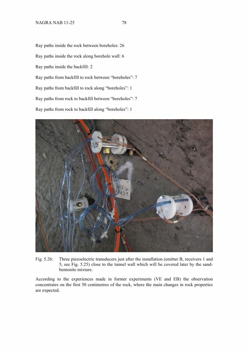
NAGRA NAB 11-25 78
Ray paths inside the rock between boreholes: 26
Ray paths inside the rock along borehole wall: 6
Ray paths inside the backfill: 2
Ray paths from backfill to rock between “boreholes”: 7
Ray paths from backfill to rock along “boreholes”: 1
Ray paths from rock to backfill between “boreholes”: 7
Ray paths from rock to backfill along “boreholes”: 1
Fig. 5.26: Three piezoelectric transducers just after the installation (emitter B, receivers 1 and 5, see Fig. 5.25) close to the tunnel wall which will be covered later by the sand-bentonite mixture.
According to the experiences made in former experiments (VE and EB) the observation concentrates on the first 50 centimetres of the rock, where the main changes in rock properties are expected.
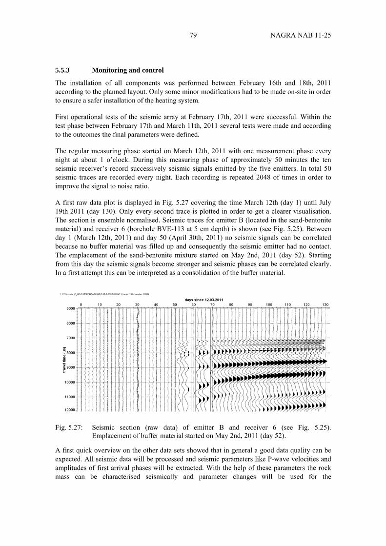
79 NAGRA NAB 11-25
5.5.3 Monitoring and control
The installation of all components was performed between February 16th and 18th, 2011 according to the planned layout. Only some minor modifications had to be made on-site in order to ensure a safer installation of the heating system.
First operational tests of the seismic array at February 17th, 2011 were successful. Within the test phase between February 17th and March 11th, 2011 several tests were made and according to the outcomes the final parameters were defined.
The regular measuring phase started on March 12th, 2011 with one measurement phase every night at about 1 o’clock. During this measuring phase of approximately 50 minutes the ten seismic receiver’s record successively seismic signals emitted by the five emitters. In total 50 seismic traces are recorded every night. Each recording is repeated 2048 of times in order to improve the signal to noise ratio.
A first raw data plot is displayed in Fig. 5.27 covering the time March 12th (day 1) until July 19th 2011 (day 130). Only every second trace is plotted in order to get a clearer visualisation. The section is ensemble normalised. Seismic traces for emitter B (located in the sand-bentonite material) and receiver 6 (borehole BVE-113 at 5 cm depth) is shown (see Fig. 5.25). Between day 1 (March 12th, 2011) and day 50 (April 30th, 2011) no seismic signals can be correlated because no buffer material was filled up and consequently the seismic emitter had no contact. The emplacement of the sand-bentonite mixture started on May 2nd, 2011 (day 52). Starting from this day the seismic signals become stronger and seismic phases can be correlated clearly. In a first attempt this can be interpreted as a consolidation of the buffer material.
Fig. 5.27: Seismic section (raw data) of emitter B and receiver 6 (see Fig. 5.25). Emplacement of buffer material started on May 2nd, 2011 (day 52).
A first quick overview on the other data sets showed that in general a good data quality can be expected. All seismic data will be processed and seismic parameters like P-wave velocities and amplitudes of first arrival phases will be extracted. With the help of these parameters the rock mass can be characterised seismically and parameter changes will be used for the
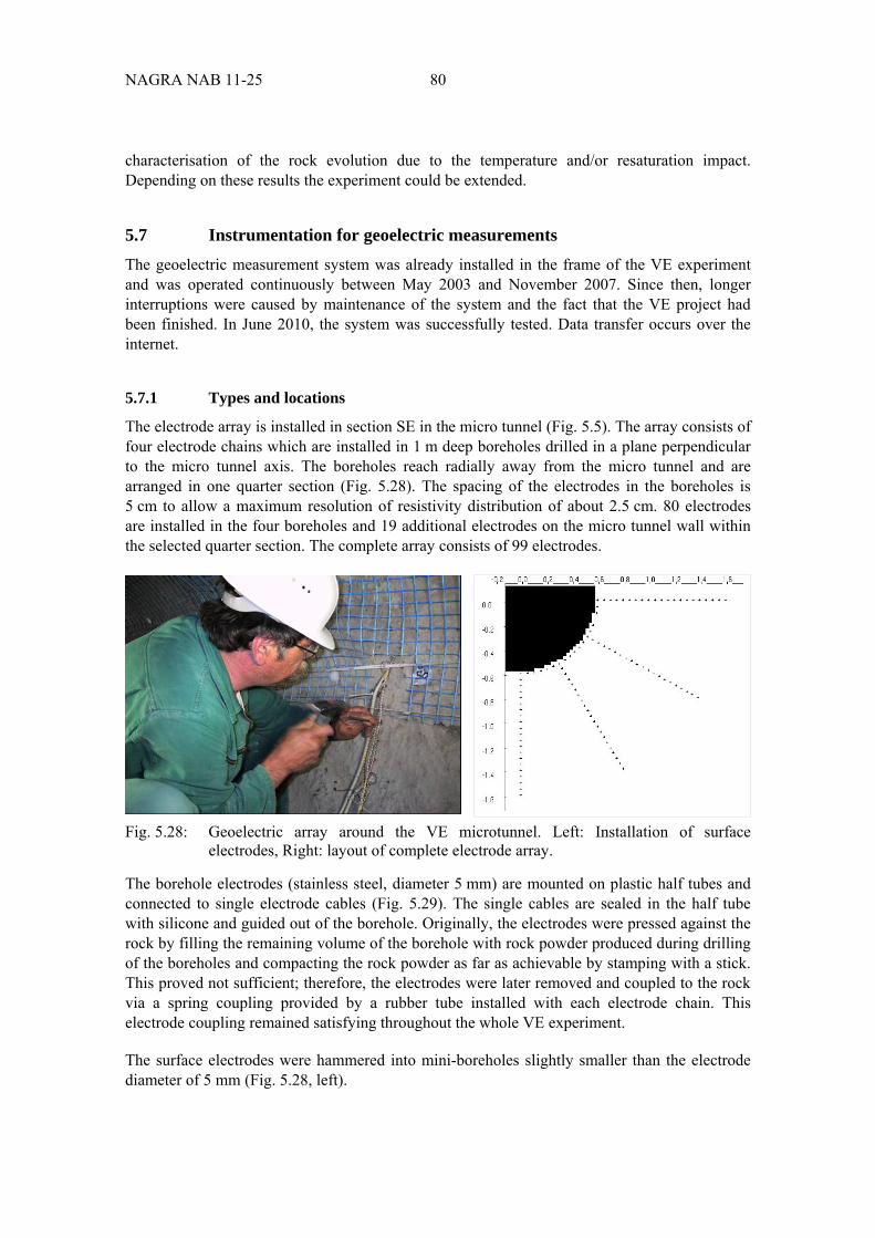
NAGRA NAB 11-25 80
characterisation of the rock evolution due to the temperature and/or resaturation impact. Depending on these results the experiment could be extended.
5.7 Instrumentation for geoelectric measurements
The geoelectric measurement system was already installed in the frame of the VE experiment and was operated continuously between May 2003 and November 2007. Since then, longer interruptions were caused by maintenance of the system and the fact that the VE project had been finished. In June 2010, the system was successfully tested. Data transfer occurs over the internet.
5.7.1 Types and locations
The electrode array is installed in section SE in the micro tunnel (Fig. 5.5). The array consists of four electrode chains which are installed in 1 m deep boreholes drilled in a plane perpendicular to the micro tunnel axis. The boreholes reach radially away from the micro tunnel and are arranged in one quarter section (Fig. 5.28). The spacing of the electrodes in the boreholes is 5 cm to allow a maximum resolution of resistivity distribution of about 2.5 cm. 80 electrodes are installed in the four boreholes and 19 additional electrodes on the micro tunnel wall within the selected quarter section. The complete array consists of 99 electrodes.
Fig. 5.28: Geoelectric array around the VE microtunnel. Left: Installation of surface electrodes, Right: layout of complete electrode array.
The borehole electrodes (stainless steel, diameter 5 mm) are mounted on plastic half tubes and connected to single electrode cables (Fig. 5.29). The single cables are sealed in the half tube with silicone and guided out of the borehole. Originally, the electrodes were pressed against the rock by filling the remaining volume of the borehole with rock powder produced during drilling of the boreholes and compacting the rock powder as far as achievable by stamping with a stick. This proved not sufficient; therefore, the electrodes were later removed and coupled to the rock via a spring coupling provided by a rubber tube installed with each electrode chain. This electrode coupling remained satisfying throughout the whole VE experiment.
The surface electrodes were hammered into mini-boreholes slightly smaller than the electrode diameter of 5 mm (Fig. 5.28, left).
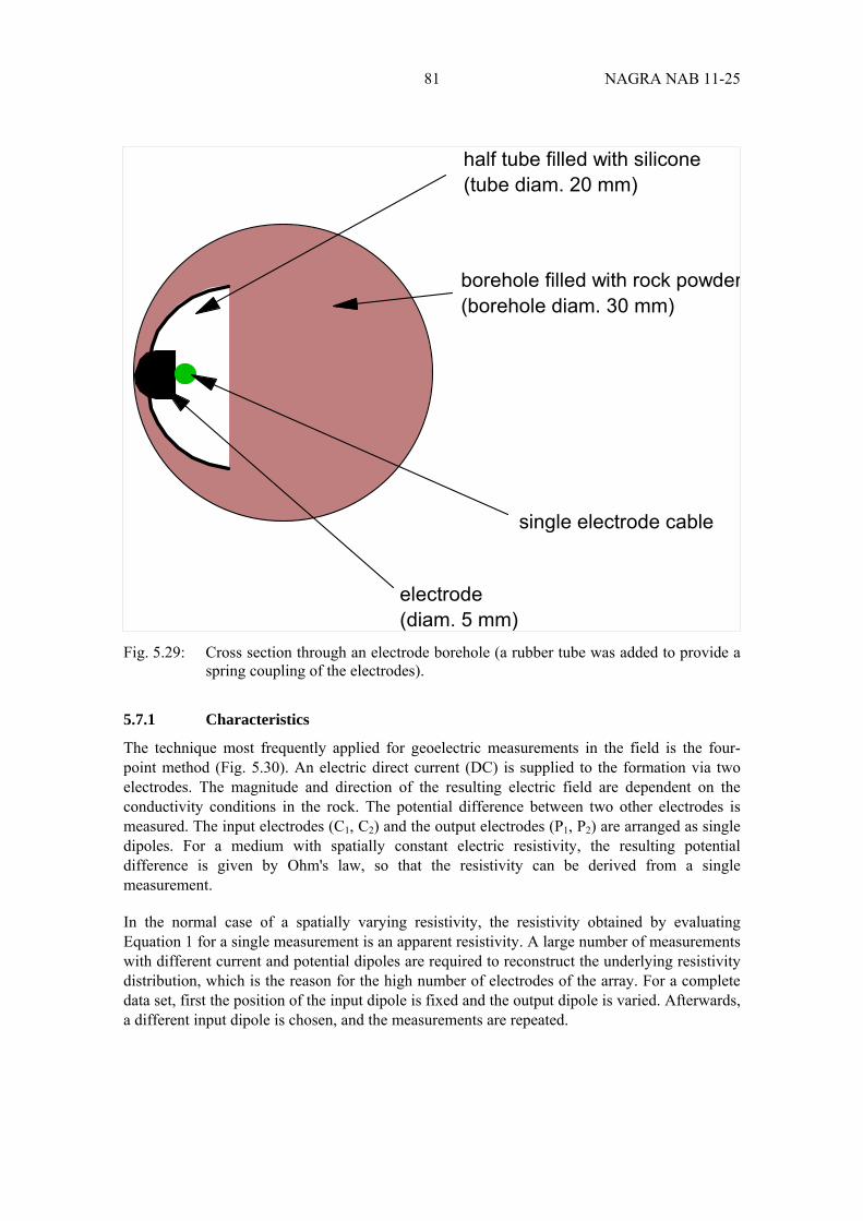
81 NAGRA NAB 11-25
Fig. 5.29: Cross section through an electrode borehole (a rubber tube was added to provide a spring coupling of the electrodes).
5.7.1 Characteristics
The technique most frequently applied for geoelectric measurements in the field is the four-point method (Fig. 5.30). An electric direct current (DC) is supplied to the formation via two electrodes. The magnitude and direction of the resulting electric field are dependent on the conductivity conditions in the rock. The potential difference between two other electrodes is measured. The input electrodes (C1, C2) and the output electrodes (P1, P2) are arranged as single dipoles. For a medium with spatially constant electric resistivity, the resulting potential difference is given by Ohm's law, so that the resistivity can be derived from a single measurement.
In the normal case of a spatially varying resistivity, the resistivity obtained by evaluating Equation 1 for a single measurement is an apparent resistivity. A large number of measurements with different current and potential dipoles are required to reconstruct the underlying resistivity distribution, which is the reason for the high number of electrodes of the array. For a complete data set, first the position of the input dipole is fixed and the output dipole is varied. Afterwards, a different input dipole is chosen, and the measurements are repeated.
borehole filled with rock powder(borehole diam. 30 mm)
half tube filled with silicone(tube diam. 20 mm)
electrode(diam. 5 mm)
single electrode cable
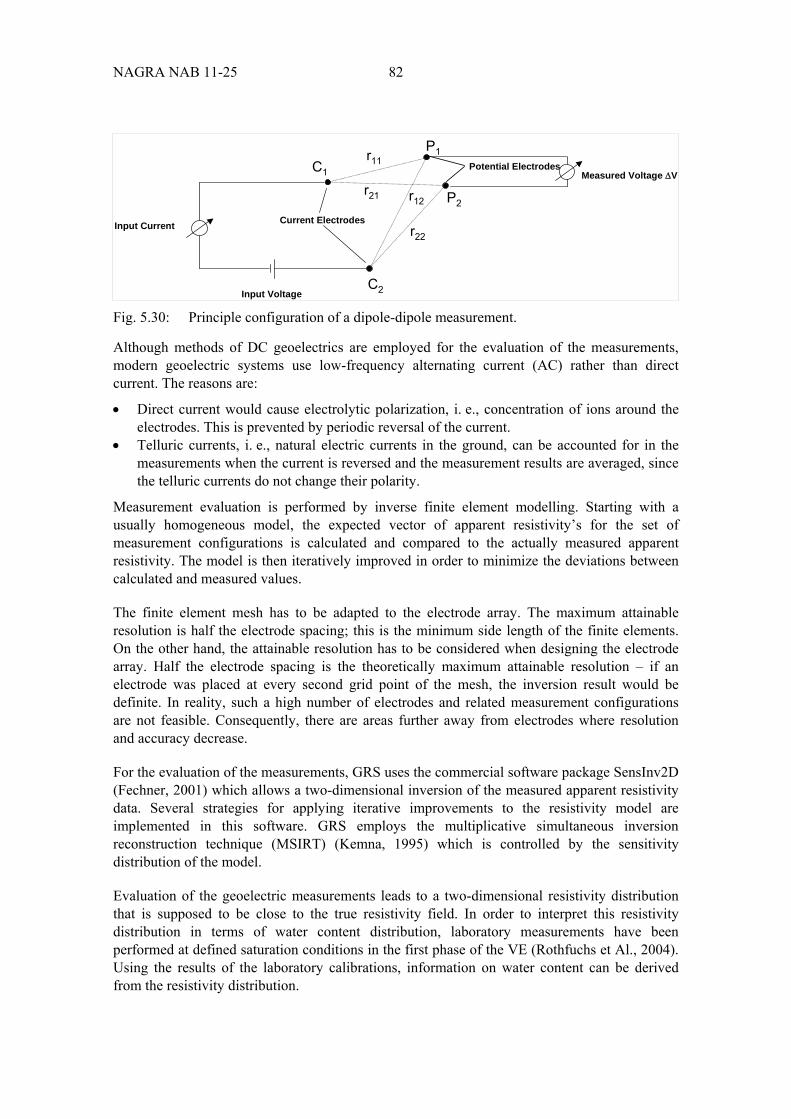
NAGRA NAB 11-25 82
Fig. 5.30: Principle configuration of a dipole-dipole measurement.
Although methods of DC geoelectrics are employed for the evaluation of the measurements, modern geoelectric systems use low-frequency alternating current (AC) rather than direct current. The reasons are:
Direct current would cause electrolytic polarization, i. e., concentration of ions around the electrodes. This is prevented by periodic reversal of the current.
Telluric currents, i. e., natural electric currents in the ground, can be accounted for in the measurements when the current is reversed and the measurement results are averaged, since the telluric currents do not change their polarity.
Measurement evaluation is performed by inverse finite element modelling. Starting with a usually homogeneous model, the expected vector of apparent resistivity’s for the set of measurement configurations is calculated and compared to the actually measured apparent resistivity. The model is then iteratively improved in order to minimize the deviations between calculated and measured values.
The finite element mesh has to be adapted to the electrode array. The maximum attainable resolution is half the electrode spacing; this is the minimum side length of the finite elements. On the other hand, the attainable resolution has to be considered when designing the electrode array. Half the electrode spacing is the theoretically maximum attainable resolution – if an electrode was placed at every second grid point of the mesh, the inversion result would be definite. In reality, such a high number of electrodes and related measurement configurations are not feasible. Consequently, there are areas further away from electrodes where resolution and accuracy decrease.
For the evaluation of the measurements, GRS uses the commercial software package SensInv2D (Fechner, 2001) which allows a two-dimensional inversion of the measured apparent resistivity data. Several strategies for applying iterative improvements to the resistivity model are implemented in this software. GRS employs the multiplicative simultaneous inversion reconstruction technique (MSIRT) (Kemna, 1995) which is controlled by the sensitivity distribution of the model.
Evaluation of the geoelectric measurements leads to a two-dimensional resistivity distribution that is supposed to be close to the true resistivity field. In order to interpret this resistivity distribution in terms of water content distribution, laboratory measurements have been performed at defined saturation conditions in the first phase of the VE (Rothfuchs et Al., 2004). Using the results of the laboratory calibrations, information on water content can be derived from the resistivity distribution.
r11C1
C2
P1
P2
Current Electrodes
Potential Electrodes
r21 r12
r22Input Current
Measured Voltage V
Input Voltage
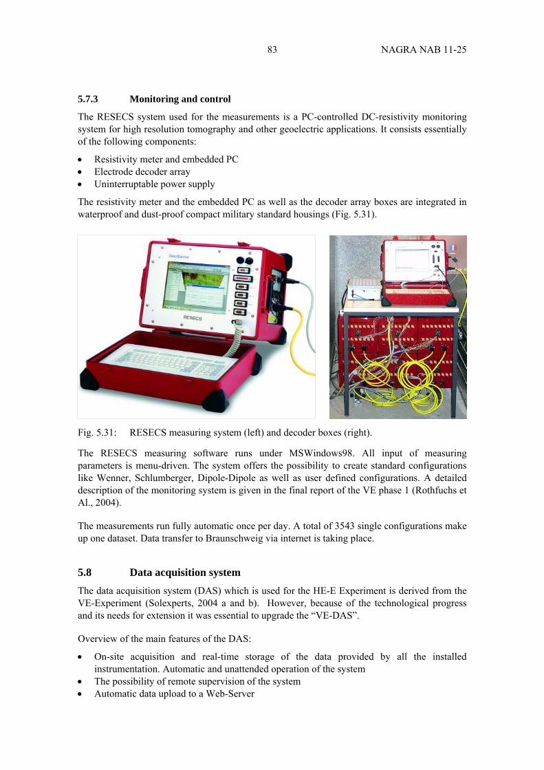
83 NAGRA NAB 11-25
5.7.3 Monitoring and control
The RESECS system used for the measurements is a PC-controlled DC-resistivity monitoring system for high resolution tomography and other geoelectric applications. It consists essentially of the following components:
Resistivity meter and embedded PC Electrode decoder array Uninterruptable power supply
The resistivity meter and the embedded PC as well as the decoder array boxes are integrated in waterproof and dust-proof compact military standard housings (Fig. 5.31).
Fig. 5.31: RESECS measuring system (left) and decoder boxes (right).
The RESECS measuring software runs under MSWindows98. All input of measuring parameters is menu-driven. The system offers the possibility to create standard configurations like Wenner, Schlumberger, Dipole-Dipole as well as user defined configurations. A detailed description of the monitoring system is given in the final report of the VE phase 1 (Rothfuchs et Al., 2004).
The measurements run fully automatic once per day. A total of 3543 single configurations make up one dataset. Data transfer to Braunschweig via internet is taking place.
5.8 Data acquisition system
The data acquisition system (DAS) which is used for the HE-E Experiment is derived from the VE-Experiment (Solexperts, 2004 a and b). However, because of the technological progress and its needs for extension it was essential to upgrade the “VE-DAS”.
Overview of the main features of the DAS:
On-site acquisition and real-time storage of the data provided by all the installed instrumentation. Automatic and unattended operation of the system
The possibility of remote supervision of the system Automatic data upload to a Web-Server

NAGRA NAB 11-25 84
Alarm and control functions Automatic backup of the data Web-based data visualisation.
The System includes the following items for robustness and consistency:
Use of industrial grade electronics for the data acquisition and computer systems (similar to the ones used at the Grimsel Test Site GTS).
PC protected with an intelligent watchdog device. Uninterrupted Power Supply (UPS) with protection against under voltage and power surges. Robust and well tested data communication hardware and software. Automatic data backup systems.
Requirements due to the system structure:
Two different data acquisition systems are required to monitor the sensors to be installed:
GeoMonitor system for the sensors with analogue output signals Psychrometer data acquisition system for the psychrometer sensors, which have a different
signal character and therefore require a separate data acquisition system, a separate signal control and storage software. The system will be the same as during the VE-Experiment since no further psychrometer sensors were added and the control program is running under DOS operational system. The system was implemented by Aitemin during the VE-Experiment.
5.8.1 GeoMonitor II System
The Solexperts GeoMonitorII data acquisition system is used to monitor the following sensors:
the sensors in the EBS and on the host rock/EBS interface all sensors in the Opalinus clay apart from the seismic and geoelectric sensors The
psychrometers are logged with the Campbell Scientific CR-7 logger but the signal is then transferred to the Geomonitor
the temperature sensors and power from the heaters (only for monitoring purposes).
An overview of all sensors connected to the DAS is given in Tab. A.3.1 – Appendix 3.
The GeoMonitorII DAS consists of an ADAM 5000 system, which was used during the VE-Experiment and which was extended for the HE-E Experiment. The signals are controlled and recorded with the GeoMonitor software. The proper functioning is controlled by an intelligent watchdog which performs automatic and/or semi-automatic system resets in case of failures. Details of the system features are listed below:
On-site data acquisition, conversion, visualisation and real-time storage of data provided by the installed instruments.
Visualization of a maximum of 20 sensors in real time in one graph. Integrated SQL database (automatically configured, no additional software packages
required); possibility of data output in ASCII or Excel format. Possibility of GeoMonitor customized alarm features, which may generate alarm notices
which are then distributed by e-mail, SMS or Fax. The recorded measurements include the date and time as well as an event code that provides
information about measurement errors, measurement values exceeding their valid range and alarm limits.
85 NAGRA NAB 11-25
The user can create entries into a logbook. The logbook report can be filtered to show only selected events. The report can be exported as an Excel spread sheet or a RTF document and imported into other word processors (WordPad, MS Word, etc).
Virtual real-time calculations of sensors including custom expressions, statistical values, delta values, etc.
Remote operation from the office using an internet. Robust design for field site conditions. The system is password protected, thus only users with the proper user rights are able to
modify the program setup.
5.8.2 Remote control system
The remote control system enables the test engineer to control the DAS software of both systems (GeoMonitor) from distance during unattended tests. The principal external communication line is the broadband internet connection. The internet signal is distributed through a router which is operated and administrated by Swisstopo. The PC may be reset over the internet line.
5.8.3 Backup systems and redundancy
An intelligent watchdog, uninterruptible power supplies (UPS); automatic data backup software and software alarms are incorporated into the DAS to assure the proper operation of the DAS and continuous data acquisition.
The system automatically monitors the different communication lines between the interfaces and the PC (internal). The internal lines will be reset automatically by the intelligent watchdog in case of internal communication problems. System resets can be performed remotely through a phone line activating the watchdog switch.
In case of power failure, the integrated UPS buffer is sufficient to power the DAS during a minimum time period of about 30 minutes. One DAS channel monitors the power line. If the power fails this channel triggers an alarm in GeoMonitor. Subsequently, an alarm message is sent to the responsible site engineer (e-mail and SMS) and the PC will shut down automatically before the UPS runs out of power. (Note: for the alarm messages the internet connection needs to be active at all times). In addition, the UPS provides voltage surge protection and brown-out (low voltage) protection.
5.8.4 WebDAVIS
WebDAVIS is a web based data visualisation and information platform for projects in geomatics, geotechnics and hydrogeology. It is a truly server-based implementation and representation through the Solexperts website makes it independent of the users' operating system and web browser. A WebDAVIS server is based on a state of the art relational database management system (RDBMS) in conjunction with a fast, reliable and secure web server.
WebDAVIS offers near-real-time viewing (couple of minutes delay) of the DAS raw and analysed data, graphics, alarm status and events from around the world via a web browser on the internet.
The WebDAVIS project site is password protected and secure. The site is designed according to the needs of the client and all needed graphs to represent the data and to enable fast and accurate

NAGRA NAB 11-25 86
monitoring of the measurements are accessible simply by clicking on interactive symbols. Thus no add-ins are required. No ports need to be opened.
The sensor positions are displayed together with their alarm and warning status. Alarms are easily identified by the colour; the current measurement is displayed. Clicking on the sensors brings up a window with details of the alarm event and the actions.
Interactive symbols provide access to predefined charts with real time access to the WebDAVIS data base to keep track of the measurements.
The graphic tool allows creating individual time charts. The graphic tool provides three main functions:
Creating customised graphs Saving and printing of these graphs Exporting of the displayed data into an ASCII text format or a spread sheet.
The recent measurements can also be viewed in table format together with the alarm status and pre-defined delta values.
Meta data including event and alarm logs from the monitoring system and from the customer together with further information on the project are always available.
Through a protected download area, information can be distributed to the different users.
On the WEBdavies the sensors of the HE-E experiment are organised in four categories:
Sensors in the EBS systems Sensors in the cross sections through the micro tunnel Sensors at a large distance from the micro tunnel Sensors from the heating system.
87 NAGRA NAB 11-25
6 Experiment as-built
On 1st of March 2011 the construction of the HE-E experiment started by emplacing plug #1. Plug #3 was completed by the 2nd of May 2011 the heaters were started on the 28th June 2011.
The construction sequence can be summarized as follows: a) construction of plug #1; b) emplacement of the bentonite blocks, first instrumentation module and liner; c) filling of the bentonite section; d) construction of plug #2; e) emplacement of the bentonite blocks, second instrumentation module and liner; f) filling of the sand/bentonite section; g) construction of plug #3; h) installation of the heaters.
Main issues encountered during the construction of the experiment regarded the cracking of the bentonite blocks in the bentonite section before bentonite filling started and difficulty to pull the heater in its correct position; but these problems didn’t obstacle the completion of the construction.
6.1 Plugs
Three plugs were constructed in the HE-E experiment: plug #1 at the bottom end of the experiment; plug #2 as separation between the granular bentonite from the sand/bentonite section; plug #3 isolates the experiment from the atmospheric conditions.
6.1.1 Location of the plugs inside the RB micro tunnel
For the HE-E experiment it has been decided to reutilize the instrumentation of the previous VE test. The SA3 section was selected to be the middle of the HE-E experiment (Fig. 6.1) and the positions of plug #1, SA3, plug #3 were marked during the site preparation activities (Fig. 2.11) in accordance to the design phase (Gaus (Ed.), 2011 – NAB11-01).
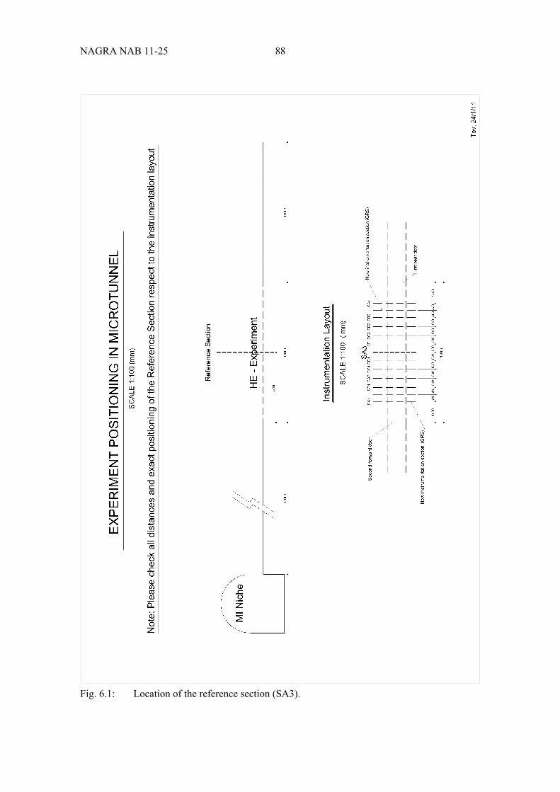
NAGRA NAB 11-25 88
Fig. 6.1: Location of the reference section (SA3).

89 NAGRA NAB 11-25
6.1.2 Properties, dimensions and installation of the plugs
Slight changes respect to the design occurred during the field works, but the construction sequence of the three plugs remained intact and was as follows:
Plug #1 (thickness 960mm), see Figs. 6.2 – 6.3
a. back end wall (cement bricks and mortar)
b. vapour barrier (aluminium foil)
c. thermal isolation (Rockwool)
d. dying end scaffolding wall for block (cement bricks and mortar)
e. block (concrete)
f. front scaffolding wall for block (cement bricks and mortar)
Plug #2 (thickness 550mm), see Figs. 6.4 – 6.5
a. back end wall for containment of bentonite material (cement bricks and mortar)
b. vapour barrier (aluminium foil)
c. thermal isolation (Rockwool)
d. vapour barrier (aluminium foil)
e. front wall (cement bricks and mortar)
Plug #3 (thickness 1090mm), see Figs. 6.6 – 6.7
a. back end wall for containment of sand/bentonite material (cement bricks and mortar)
b. thermal isolation (Rockwool)
c. vapour barrier (aluminium foil)
d. dying end scaffolding wall for block (cement bricks and mortar)
e. block (concrete)
f. front scaffolding wall for block (cement bricks and mortar)
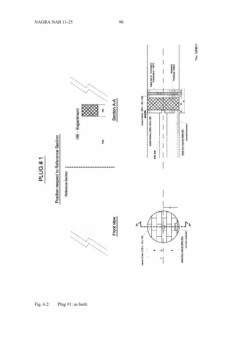
NAGRA NAB 11-25 90
Fig. 6.2: Plug #1: as built.
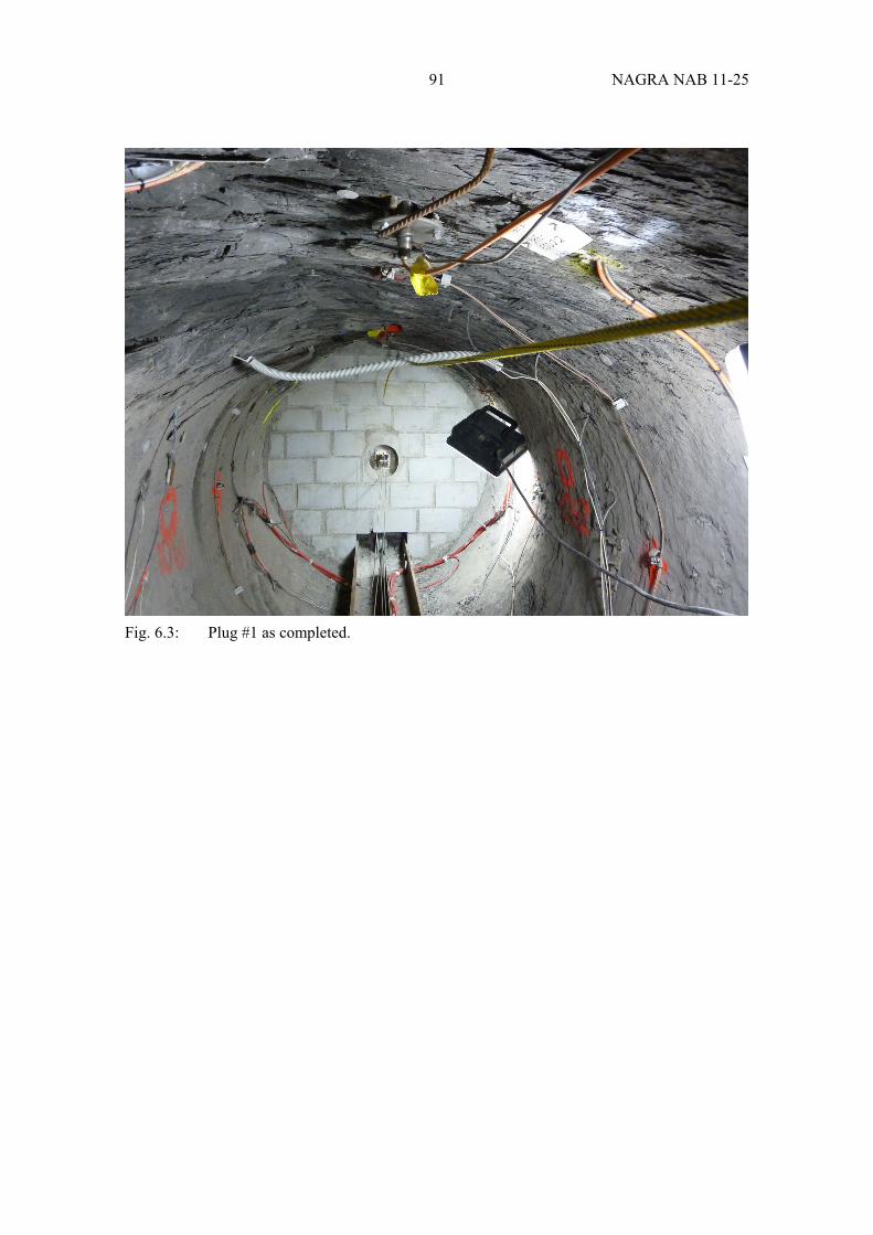
91 NAGRA NAB 11-25
Fig. 6.3: Plug #1 as completed.
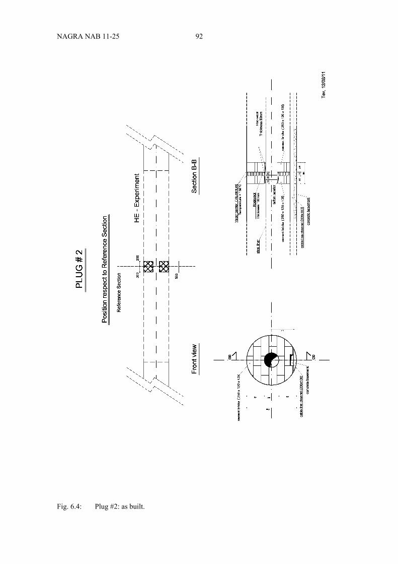
NAGRA NAB 11-25 92
Fig. 6.4: Plug #2: as built.
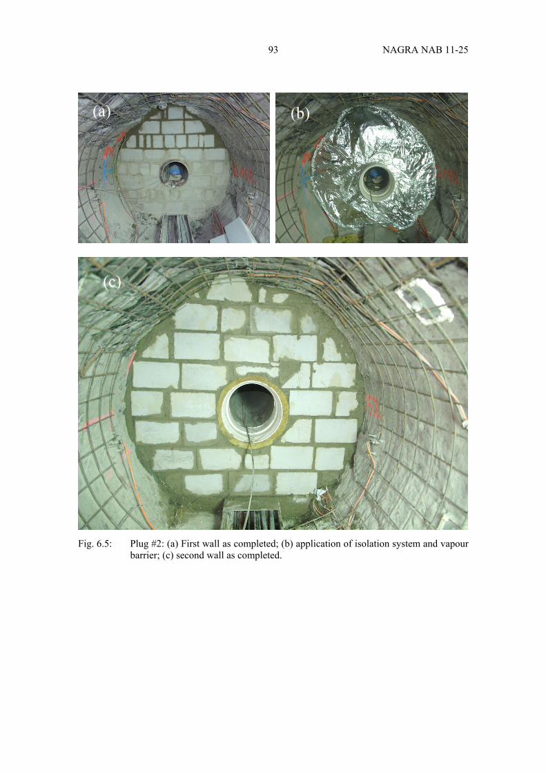
93 NAGRA NAB 11-25
Fig. 6.5: Plug #2: (a) First wall as completed; (b) application of isolation system and vapour barrier; (c) second wall as completed.
(c)
(a) (b)
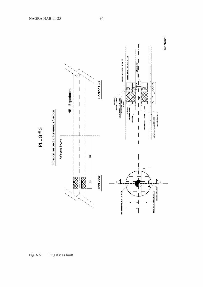
NAGRA NAB 11-25 94
Fig. 6.6: Plug #3: as built.
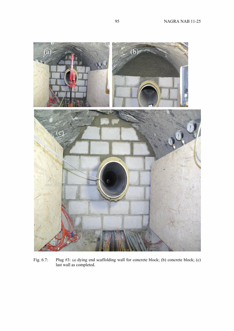
95 NAGRA NAB 11-25
Fig. 6.7: Plug #3: (a) dying end scaffolding wall for concrete block; (b) concrete block; (c) last wall as completed.
(c)
(b) (a)
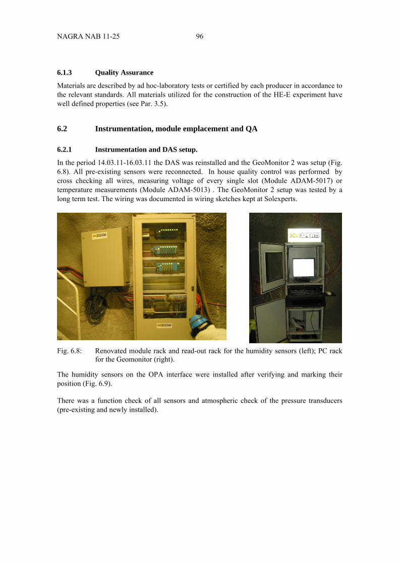
NAGRA NAB 11-25 96
6.1.3 Quality Assurance
Materials are described by ad hoc-laboratory tests or certified by each producer in accordance to the relevant standards. All materials utilized for the construction of the HE-E experiment have well defined properties (see Par. 3.5).
6.2 Instrumentation, module emplacement and QA
6.2.1 Instrumentation and DAS setup.
In the period 14.03.11-16.03.11 the DAS was reinstalled and the GeoMonitor 2 was setup (Fig. 6.8). All pre-existing sensors were reconnected. In house quality control was performed by cross checking all wires, measuring voltage of every single slot (Module ADAM-5017) or temperature measurements (Module ADAM-5013) . The GeoMonitor 2 setup was tested by a long term test. The wiring was documented in wiring sketches kept at Solexperts.
Fig. 6.8: Renovated module rack and read-out rack for the humidity sensors (left); PC rack for the Geomonitor (right).
The humidity sensors on the OPA interface were installed after verifying and marking their position (Fig. 6.9).
There was a function check of all sensors and atmospheric check of the pressure transducers (pre-existing and newly installed).
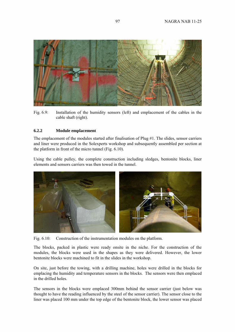
97 NAGRA NAB 11-25
Fig. 6.9: Installation of the humidity sensors (left) and emplacement of the cables in the cable shaft (right).
6.2.2 Module emplacement
The emplacement of the modules started after finalisation of Plug #1. The slides, sensor carriers and liner were produced in the Solexperts workshop and subsequently assembled per section at the platform in front of the micro tunnel (Fig. 6.10).
Using the cable pulley, the complete construction including sledges, bentonite blocks, liner elements and sensors carriers was then towed in the tunnel.
Fig. 6.10: Construction of the instrumentation modules on the platform.
The blocks, packed in plastic were ready onsite in the niche. For the construction of the modules, the blocks were used in the shapes as they were delivered. However, the lower bentonite blocks were machined to fit in the slides in the workshop.
On site, just before the towing, with a drilling machine, holes were drilled in the blocks for emplacing the humidity and temperature sensors in the blocks. The sensors were then emplaced in the drilled holes.
The sensors in the blocks were emplaced 300mm behind the sensor carrier (just below was thought to have the reading influenced by the steel of the sensor carrier). The sensor close to the liner was placed 100 mm under the top edge of the bentonite block, the lower sensor was placed
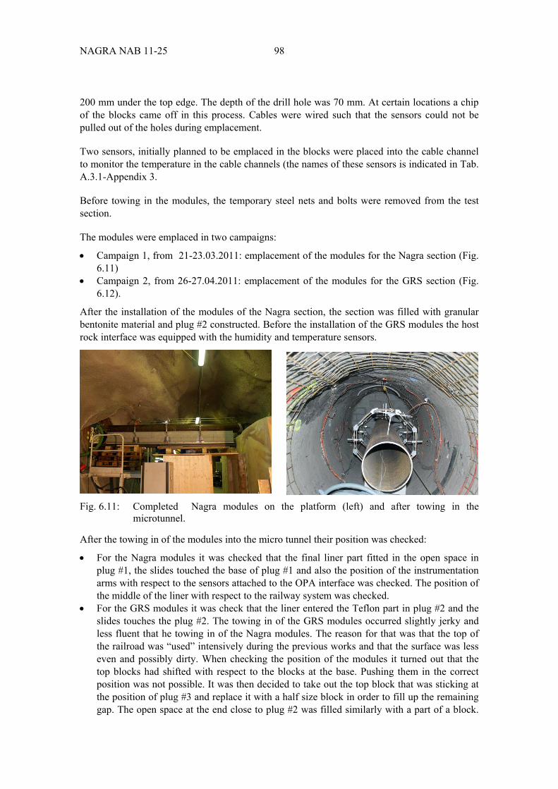
NAGRA NAB 11-25 98
200 mm under the top edge. The depth of the drill hole was 70 mm. At certain locations a chip of the blocks came off in this process. Cables were wired such that the sensors could not be pulled out of the holes during emplacement.
Two sensors, initially planned to be emplaced in the blocks were placed into the cable channel to monitor the temperature in the cable channels (the names of these sensors is indicated in Tab. A.3.1-Appendix 3.
Before towing in the modules, the temporary steel nets and bolts were removed from the test section.
The modules were emplaced in two campaigns:
Campaign 1, from 21-23.03.2011: emplacement of the modules for the Nagra section (Fig. 6.11)
Campaign 2, from 26-27.04.2011: emplacement of the modules for the GRS section (Fig. 6.12).
After the installation of the modules of the Nagra section, the section was filled with granular bentonite material and plug #2 constructed. Before the installation of the GRS modules the host rock interface was equipped with the humidity and temperature sensors.
Fig. 6.11: Completed Nagra modules on the platform (left) and after towing in the microtunnel.
After the towing in of the modules into the micro tunnel their position was checked:
For the Nagra modules it was checked that the final liner part fitted in the open space in plug #1, the slides touched the base of plug #1 and also the position of the instrumentation arms with respect to the sensors attached to the OPA interface was checked. The position of the middle of the liner with respect to the railway system was checked.
For the GRS modules it was check that the liner entered the Teflon part in plug #2 and the slides touches the plug #2. The towing in of the GRS modules occurred slightly jerky and less fluent that he towing in of the Nagra modules. The reason for that was that the top of the railroad was “used” intensively during the previous works and that the surface was less even and possibly dirty. When checking the position of the modules it turned out that the top blocks had shifted with respect to the blocks at the base. Pushing them in the correct position was not possible. It was then decided to take out the top block that was sticking at the position of plug #3 and replace it with a half size block in order to fill up the remaining gap. The open space at the end close to plug #2 was filled similarly with a part of a block.
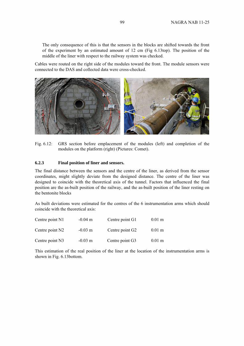
99 NAGRA NAB 11-25
The only consequence of this is that the sensors in the blocks are shifted towards the front of the experiment by an estimated amount of 12 cm (Fig 6.13top). The position of the middle of the liner with respect to the railway system was checked.
Cables were routed on the right side of the modules toward the front. The module sensors were connected to the DAS and collected data were cross-checked.
Fig. 6.12: GRS section before emplacement of the modules (left) and completion of the modules on the platform (right) (Pictures: Comet).
6.2.3 Final position of liner and sensors.
The final distance between the sensors and the centre of the liner, as derived from the sensor coordinates, might slightly deviate from the designed distance. The centre of the liner was designed to coincide with the theoretical axis of the tunnel. Factors that influenced the final position are the as-built position of the railway, and the as-built position of the liner resting on the bentonite blocks
As built deviations were estimated for the centres of the 6 instrumentation arms which should coincide with the theoretical axis:
Centre point N1 -0.04 m Centre point G1 0.01 m
Centre point N2 -0.03 m Centre point G2 0.01 m
Centre point N3 -0.03 m Centre point G3 0.01 m
This estimation of the real position of the liner at the location of the instrumentation arms is shown in Fig. 6.13bottom.
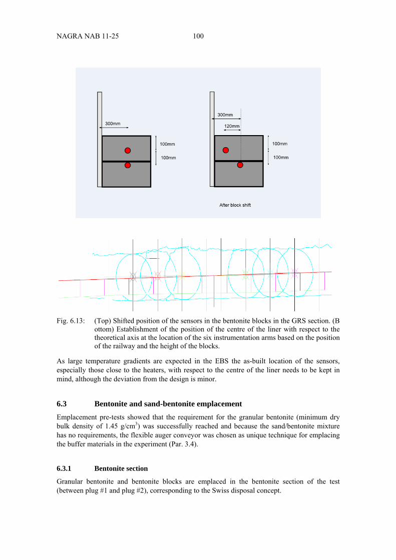
NAGRA NAB 11-25 100
Fig. 6.13: (Top) Shifted position of the sensors in the bentonite blocks in the GRS section. (B ottom) Establishment of the position of the centre of the liner with respect to the theoretical axis at the location of the six instrumentation arms based on the position of the railway and the height of the blocks.
As large temperature gradients are expected in the EBS the as-built location of the sensors, especially those close to the heaters, with respect to the centre of the liner needs to be kept in mind, although the deviation from the design is minor.
6.3 Bentonite and sand-bentonite emplacement
Emplacement pre-tests showed that the requirement for the granular bentonite (minimum dry bulk density of 1.45 g/cm3) was successfully reached and because the sand/bentonite mixture has no requirements, the flexible auger conveyor was chosen as unique technique for emplacing the buffer materials in the experiment (Par. 3.4).
6.3.1 Bentonite section
Granular bentonite and bentonite blocks are emplaced in the bentonite section of the test (between plug #1 and plug #2), corresponding to the Swiss disposal concept.
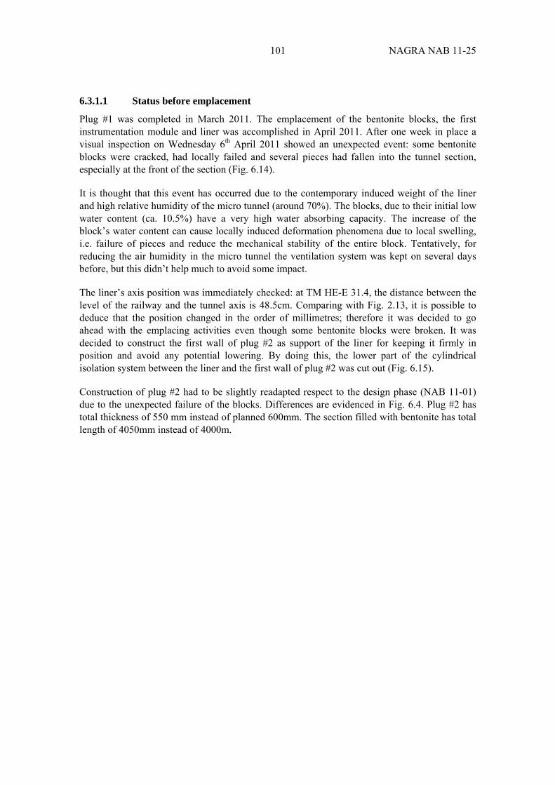
101 NAGRA NAB 11-25
6.3.1.1 Status before emplacement
Plug #1 was completed in March 2011. The emplacement of the bentonite blocks, the first instrumentation module and liner was accomplished in April 2011. After one week in place a visual inspection on Wednesday 6th April 2011 showed an unexpected event: some bentonite blocks were cracked, had locally failed and several pieces had fallen into the tunnel section, especially at the front of the section (Fig. 6.14).
It is thought that this event has occurred due to the contemporary induced weight of the liner and high relative humidity of the micro tunnel (around 70%). The blocks, due to their initial low water content (ca. 10.5%) have a very high water absorbing capacity. The increase of the block’s water content can cause locally induced deformation phenomena due to local swelling, i.e. failure of pieces and reduce the mechanical stability of the entire block. Tentatively, for reducing the air humidity in the micro tunnel the ventilation system was kept on several days before, but this didn’t help much to avoid some impact.
The liner’s axis position was immediately checked: at TM HE-E 31.4, the distance between the level of the railway and the tunnel axis is 48.5cm. Comparing with Fig. 2.13, it is possible to deduce that the position changed in the order of millimetres; therefore it was decided to go ahead with the emplacing activities even though some bentonite blocks were broken. It was decided to construct the first wall of plug #2 as support of the liner for keeping it firmly in position and avoid any potential lowering. By doing this, the lower part of the cylindrical isolation system between the liner and the first wall of plug #2 was cut out (Fig. 6.15).
Construction of plug #2 had to be slightly readapted respect to the design phase (NAB 11-01) due to the unexpected failure of the blocks. Differences are evidenced in Fig. 6.4. Plug #2 has total thickness of 550 mm instead of planned 600mm. The section filled with bentonite has total length of 4050mm instead of 4000m.
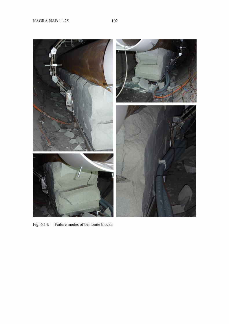
NAGRA NAB 11-25 102
Fig. 6.14: Failure modes of bentonite blocks.
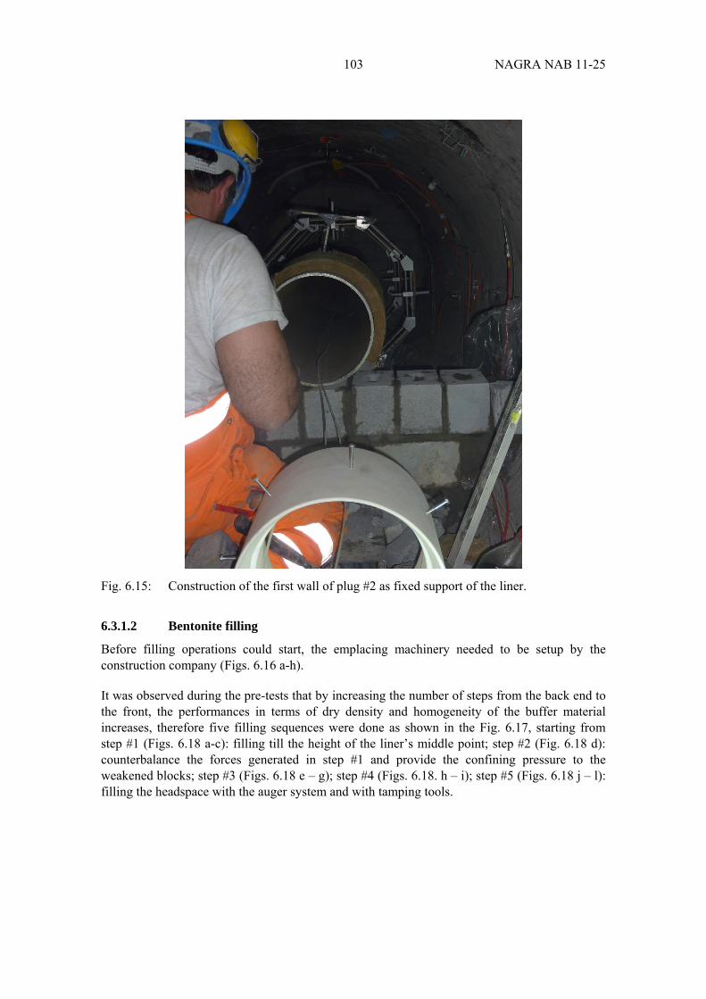
103 NAGRA NAB 11-25
Fig. 6.15: Construction of the first wall of plug #2 as fixed support of the liner.
6.3.1.2 Bentonite filling
Before filling operations could start, the emplacing machinery needed to be setup by the construction company (Figs. 6.16 a-h).
It was observed during the pre-tests that by increasing the number of steps from the back end to the front, the performances in terms of dry density and homogeneity of the buffer material increases, therefore five filling sequences were done as shown in the Fig. 6.17, starting from step #1 (Figs. 6.18 a-c): filling till the height of the liner’s middle point; step #2 (Fig. 6.18 d): counterbalance the forces generated in step #1 and provide the confining pressure to the weakened blocks; step #3 (Figs. 6.18 e – g); step #4 (Figs. 6.18. h – i); step #5 (Figs. 6.18 j – l): filling the headspace with the auger system and with tamping tools.
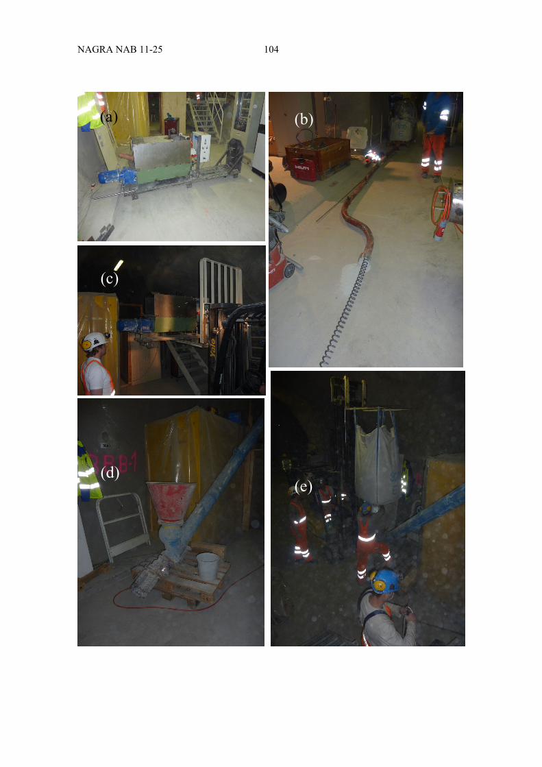
NAGRA NAB 11-25 104
(a) (b)
(c)
(d) (e)
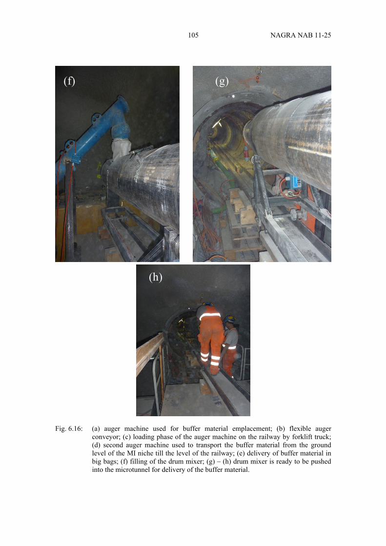
105 NAGRA NAB 11-25
Fig. 6.16: (a) auger machine used for buffer material emplacement; (b) flexible auger conveyor; (c) loading phase of the auger machine on the railway by forklift truck; (d) second auger machine used to transport the buffer material from the ground level of the MI niche till the level of the railway; (e) delivery of buffer material in big bags; (f) filling of the drum mixer; (g) – (h) drum mixer is ready to be pushed into the microtunnel for delivery of the buffer material.
(f) (g)
(h)
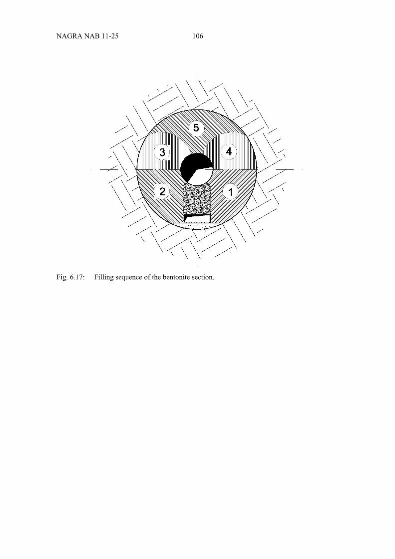
NAGRA NAB 11-25 106
Fig. 6.17: Filling sequence of the bentonite section.
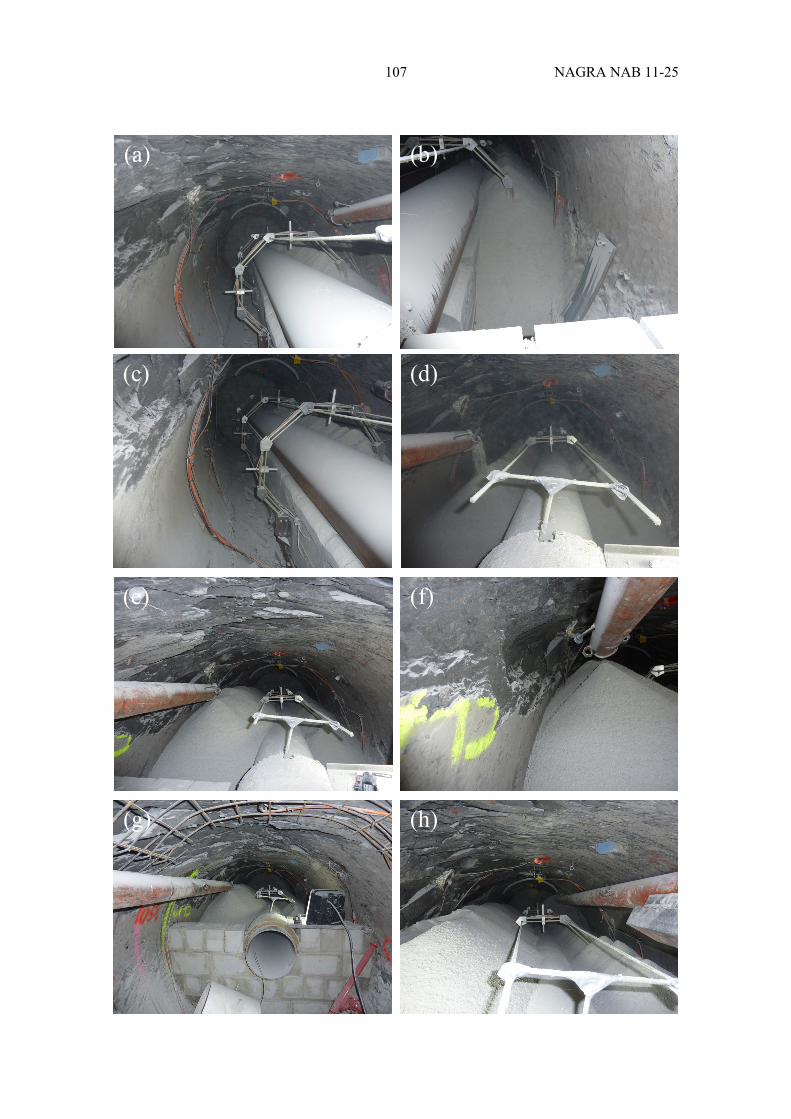
107 NAGRA NAB 11-25
(a) (b)
(c) (d)
(f) (e)
(h) (g)
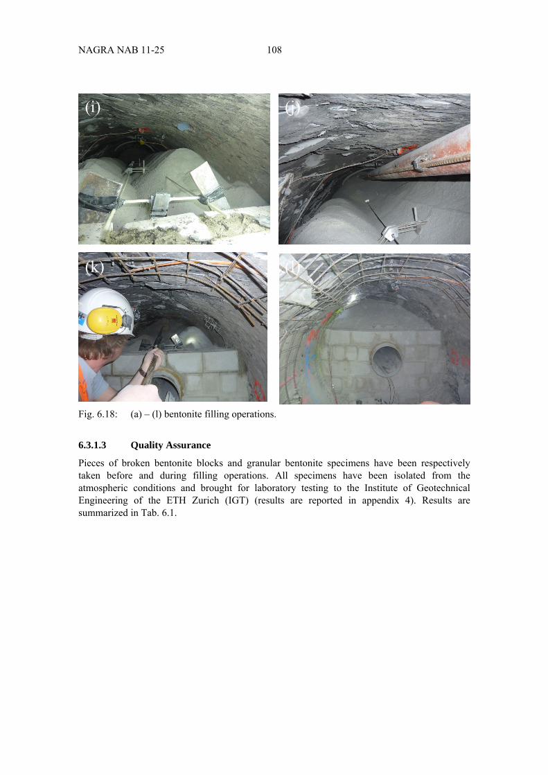
NAGRA NAB 11-25 108
Fig. 6.18: (a) – (l) bentonite filling operations.
6.3.1.3 Quality Assurance
Pieces of broken bentonite blocks and granular bentonite specimens have been respectively taken before and during filling operations. All specimens have been isolated from the atmospheric conditions and brought for laboratory testing to the Institute of Geotechnical Engineering of the ETH Zurich (IGT) (results are reported in appendix 4). Results are summarized in Tab. 6.1.
(i) (j)
(k) (l)
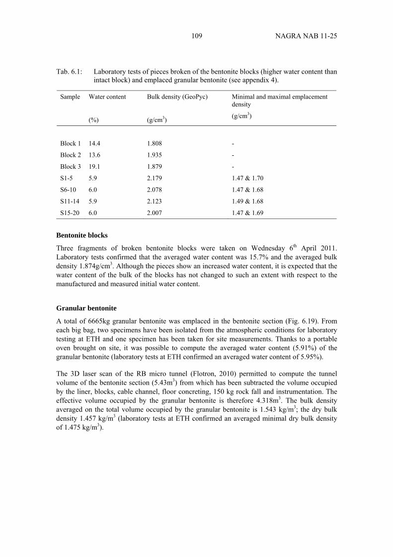
109 NAGRA NAB 11-25
Tab. 6.1: Laboratory tests of pieces broken of the bentonite blocks (higher water content than intact block) and emplaced granular bentonite (see appendix 4).
Sample Water content
(%)
Bulk density (GeoPyc)
(g/cm3)
Minimal and maximal emplacement density
(g/cm3)
Block 1 14.4 1.808 -
Block 2 13.6 1.935 -
Block 3 19.1 1.879 -
S1-5 5.9 2.179 1.47 & 1.70
S6-10 6.0 2.078 1.47 & 1.68
S11-14 5.9 2.123 1.49 & 1.68
S15-20 6.0 2.007 1.47 & 1.69
Bentonite blocks
Three fragments of broken bentonite blocks were taken on Wednesday 6th April 2011. Laboratory tests confirmed that the averaged water content was 15.7% and the averaged bulk density 1.874g/cm3. Although the pieces show an increased water content, it is expected that the water content of the bulk of the blocks has not changed to such an extent with respect to the manufactured and measured initial water content.
Granular bentonite
A total of 6665kg granular bentonite was emplaced in the bentonite section (Fig. 6.19). From each big bag, two specimens have been isolated from the atmospheric conditions for laboratory testing at ETH and one specimen has been taken for site measurements. Thanks to a portable oven brought on site, it was possible to compute the averaged water content (5.91%) of the granular bentonite (laboratory tests at ETH confirmed an averaged water content of 5.95%).
The 3D laser scan of the RB micro tunnel (Flotron, 2010) permitted to compute the tunnel volume of the bentonite section (5.43m3) from which has been subtracted the volume occupied by the liner, blocks, cable channel, floor concreting, 150 kg rock fall and instrumentation. The effective volume occupied by the granular bentonite is therefore 4.318m3. The bulk density averaged on the total volume occupied by the granular bentonite is 1.543 kg/m3; the dry bulk density 1.457 kg/m3 (laboratory tests at ETH confirmed an averaged minimal dry bulk density of 1.475 kg/m3).
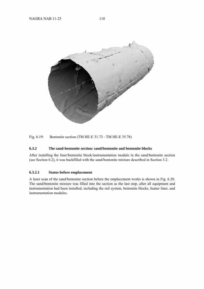
NAGRA NAB 11-25 110
Fig. 6.19: Bentonite section (TM HE-E 31.73 - TM HE-E 35.78)
6.3.2 The sand-bentonite section: sand/bentonite and bentonite blocks
After installing the liner/bentonite block/instrumentation module in the sand/bentonite section (see Section 6.2), it was backfilled with the sand/bentonite mixture described in Section 3.2.
6.3.2.1 Status before emplacement
A laser scan of the sand/bentonite section before the emplacement works is shown in Fig. 6.20. The sand/bentonite mixture was filled into the section as the last step, after all equipment and instrumentation had been installed, including the rail system, bentonite blocks, heater liner, and instrumentation modules.
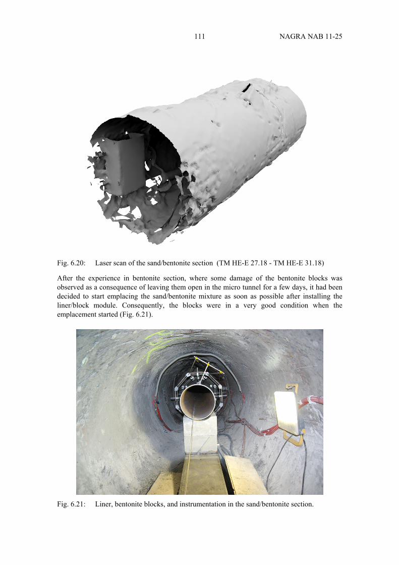
111 NAGRA NAB 11-25
Fig. 6.20: Laser scan of the sand/bentonite section (TM HE-E 27.18 - TM HE-E 31.18)
After the experience in bentonite section, where some damage of the bentonite blocks was observed as a consequence of leaving them open in the micro tunnel for a few days, it had been decided to start emplacing the sand/bentonite mixture as soon as possible after installing the liner/block module. Consequently, the blocks were in a very good condition when the emplacement started (Fig. 6.21).
Fig. 6.21: Liner, bentonite blocks, and instrumentation in the sand/bentonite section.
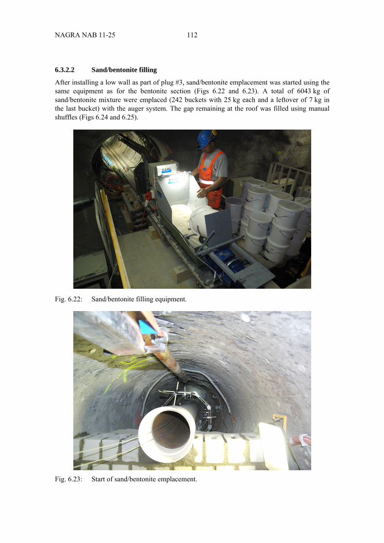
NAGRA NAB 11-25 112
6.3.2.2 Sand/bentonite filling
After installing a low wall as part of plug #3, sand/bentonite emplacement was started using the same equipment as for the bentonite section (Figs 6.22 and 6.23). A total of 6043 kg of sand/bentonite mixture were emplaced (242 buckets with 25 kg each and a leftover of 7 kg in the last bucket) with the auger system. The gap remaining at the roof was filled using manual shuffles (Figs 6.24 and 6.25).
Fig. 6.22: Sand/bentonite filling equipment.
Fig. 6.23: Start of sand/bentonite emplacement.
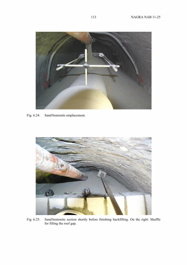
113 NAGRA NAB 11-25
Fig. 6.24: Sand/bentonite emplacement.
Fig. 6.25: Sand/bentonite section shortly before finishing backfilling. On the right: Shuffle for filling the roof gap.
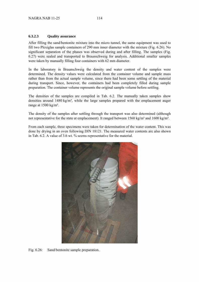
NAGRA NAB 11-25 114
6.3.2.3 Quality assurance
After filling the sand/bentonite mixture into the micro tunnel, the same equipment was used to fill two Plexiglas sample containers of 290 mm inner diameter with the mixture (Fig. 6.26). No significant separation of the phases was observed during and after filling. The samples (Fig. 6.27) were sealed and transported to Braunschweig for analysis. Additional smaller samples were taken by manually filling four containers with 62 mm diameter.
In the laboratory in Braunschweig the density and water content of the samples were determined. The density values were calculated from the container volume and sample mass rather than from the actual sample volume, since there had been some settling of the material during transport. Since, however, the containers had been completely filled during sample preparation. The container volume represents the original sample volume before settling.
The densities of the samples are compiled in Tab. 6.2. The manually taken samples show densities around 1480 kg/m³, while the large samples prepared with the emplacement auger range at 1500 kg/m³.
The density of the samples after settling through the transport was also determined (although not representative for the state at emplacement). It ranged between 1560 kg/m³ and 1600 kg/m³.
From each sample, three specimens were taken for determination of the water content. This was done by drying in an oven following DIN 18121. The measured water contents are also shown in Tab. 6.2. A value of 3.6 wt. % seems representative for the material.
Fig. 6.26: Sand/bentonite sample preparation.
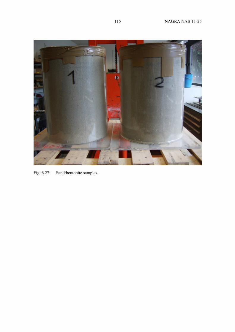
115 NAGRA NAB 11-25
Fig. 6.27: Sand/bentonite samples.
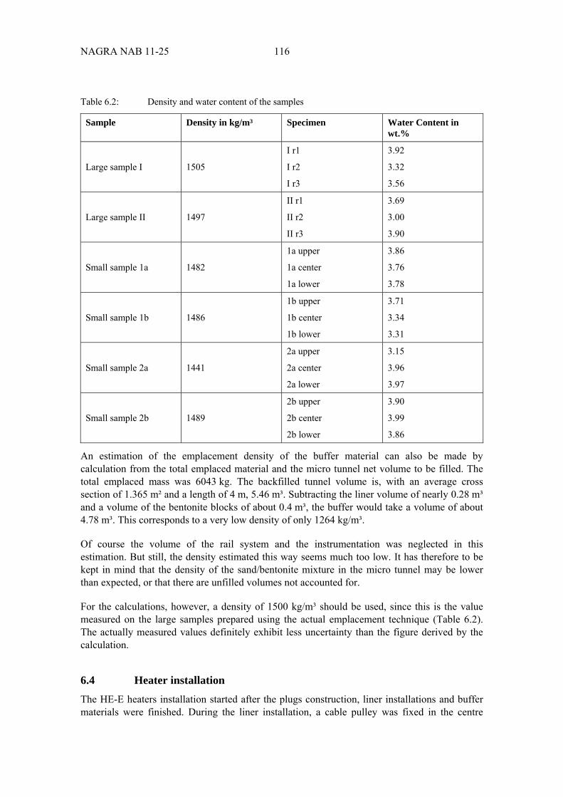
NAGRA NAB 11-25 116
Table 6.2: Density and water content of the samples
Sample Density in kg/m³ Specimen Water Content in wt.%
Large sample I
1505
I r1
I r2
I r3
3.92
3.32
3.56
Large sample II
1497
II r1
II r2
II r3
3.69
3.00
3.90
Small sample 1a
1482
1a upper
1a center
1a lower
3.86
3.76
3.78
Small sample 1b
1486
1b upper
1b center
1b lower
3.71
3.34
3.31
Small sample 2a
1441
2a upper
2a center
2a lower
3.15
3.96
3.97
Small sample 2b
1489
2b upper
2b center
2b lower
3.90
3.99
3.86
An estimation of the emplacement density of the buffer material can also be made by calculation from the total emplaced material and the micro tunnel net volume to be filled. The total emplaced mass was 6043 kg. The backfilled tunnel volume is, with an average cross section of 1.365 m² and a length of 4 m, 5.46 m³. Subtracting the liner volume of nearly 0.28 m³ and a volume of the bentonite blocks of about 0.4 m³, the buffer would take a volume of about 4.78 m³. This corresponds to a very low density of only 1264 kg/m³.
Of course the volume of the rail system and the instrumentation was neglected in this estimation. But still, the density estimated this way seems much too low. It has therefore to be kept in mind that the density of the sand/bentonite mixture in the micro tunnel may be lower than expected, or that there are unfilled volumes not accounted for.
For the calculations, however, a density of 1500 kg/m³ should be used, since this is the value measured on the large samples prepared using the actual emplacement technique (Table 6.2). The actually measured values definitely exhibit less uncertainty than the figure derived by the calculation.
6.4 Heater installation
The HE-E heaters installation started after the plugs construction, liner installations and buffer materials were finished. During the liner installation, a cable pulley was fixed in the centre
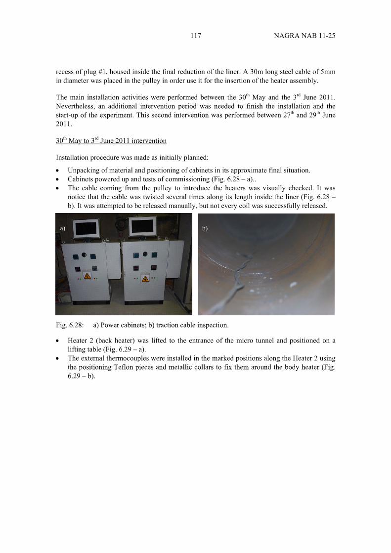
117 NAGRA NAB 11-25
recess of plug #1, housed inside the final reduction of the liner. A 30m long steel cable of 5mm in diameter was placed in the pulley in order use it for the insertion of the heater assembly.
The main installation activities were performed between the 30th May and the 3rd June 2011. Nevertheless, an additional intervention period was needed to finish the installation and the start-up of the experiment. This second intervention was performed between 27th and 29th June 2011.
30th May to 3rd June 2011 intervention
Installation procedure was made as initially planned:
Unpacking of material and positioning of cabinets in its approximate final situation. Cabinets powered up and tests of commissioning (Fig. 6.28 – a).. The cable coming from the pulley to introduce the heaters was visually checked. It was
notice that the cable was twisted several times along its length inside the liner (Fig. 6.28 – b). It was attempted to be released manually, but not every coil was successfully released.
Fig. 6.28: a) Power cabinets; b) traction cable inspection.
Heater 2 (back heater) was lifted to the entrance of the micro tunnel and positioned on a lifting table (Fig. 6.29 – a).
The external thermocouples were installed in the marked positions along the Heater 2 using the positioning Teflon pieces and metallic collars to fix them around the body heater (Fig. 6.29 – b).
a) b)
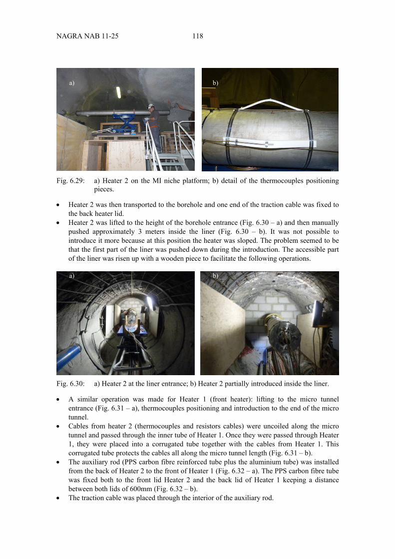
NAGRA NAB 11-25 118
Fig. 6.29: a) Heater 2 on the MI niche platform; b) detail of the thermocouples positioning pieces.
Heater 2 was then transported to the borehole and one end of the traction cable was fixed to the back heater lid.
Heater 2 was lifted to the height of the borehole entrance (Fig. 6.30 – a) and then manually pushed approximately 3 meters inside the liner (Fig. 6.30 – b). It was not possible to introduce it more because at this position the heater was sloped. The problem seemed to be that the first part of the liner was pushed down during the introduction. The accessible part of the liner was risen up with a wooden piece to facilitate the following operations.
Fig. 6.30: a) Heater 2 at the liner entrance; b) Heater 2 partially introduced inside the liner.
A similar operation was made for Heater 1 (front heater): lifting to the micro tunnel entrance (Fig. 6.31 – a), thermocouples positioning and introduction to the end of the micro tunnel.
Cables from heater 2 (thermocouples and resistors cables) were uncoiled along the micro tunnel and passed through the inner tube of Heater 1. Once they were passed through Heater 1, they were placed into a corrugated tube together with the cables from Heater 1. This corrugated tube protects the cables all along the micro tunnel length (Fig. 6.31 – b).
The auxiliary rod (PPS carbon fibre reinforced tube plus the aluminium tube) was installed from the back of Heater 2 to the front of Heater 1 (Fig. 6.32 – a). The PPS carbon fibre tube was fixed both to the front lid Heater 2 and the back lid of Heater 1 keeping a distance between both lids of 600mm (Fig. 6.32 – b).
The traction cable was placed through the interior of the auxiliary rod.
a) b)
a) b)
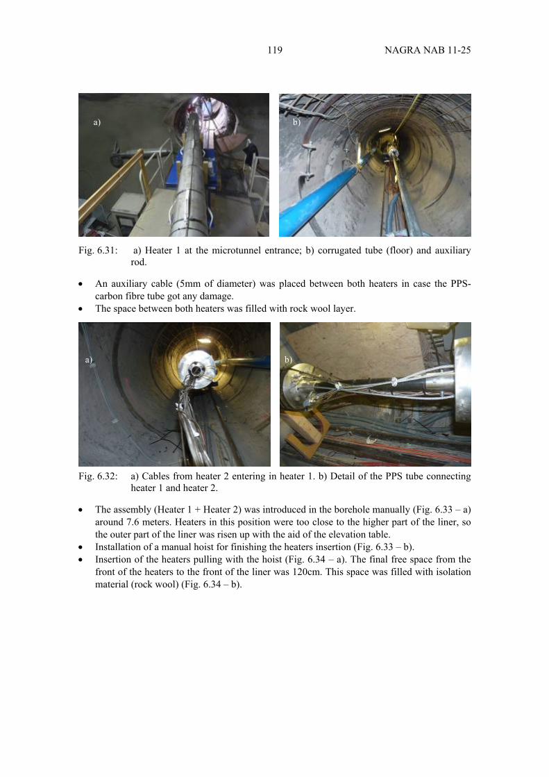
119 NAGRA NAB 11-25
Fig. 6.31: a) Heater 1 at the microtunnel entrance; b) corrugated tube (floor) and auxiliary rod.
An auxiliary cable (5mm of diameter) was placed between both heaters in case the PPS-carbon fibre tube got any damage.
The space between both heaters was filled with rock wool layer.
Fig. 6.32: a) Cables from heater 2 entering in heater 1. b) Detail of the PPS tube connecting heater 1 and heater 2.
The assembly (Heater 1 + Heater 2) was introduced in the borehole manually (Fig. 6.33 – a) around 7.6 meters. Heaters in this position were too close to the higher part of the liner, so the outer part of the liner was risen up with the aid of the elevation table.
Installation of a manual hoist for finishing the heaters insertion (Fig. 6.33 – b). Insertion of the heaters pulling with the hoist (Fig. 6.34 – a). The final free space from the
front of the heaters to the front of the liner was 120cm. This space was filled with isolation material (rock wool) (Fig. 6.34 – b).
a) b)
a) b)
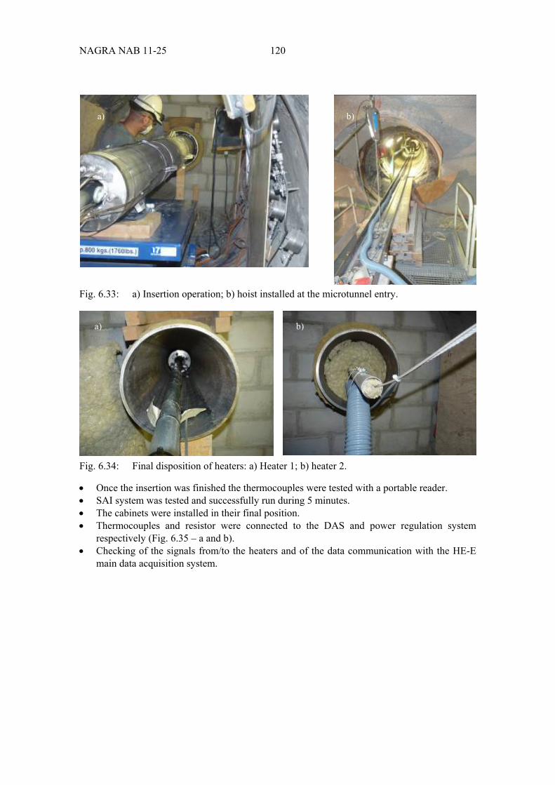
NAGRA NAB 11-25 120
Fig. 6.33: a) Insertion operation; b) hoist installed at the microtunnel entry.
Fig. 6.34: Final disposition of heaters: a) Heater 1; b) heater 2.
Once the insertion was finished the thermocouples were tested with a portable reader. SAI system was tested and successfully run during 5 minutes. The cabinets were installed in their final position. Thermocouples and resistor were connected to the DAS and power regulation system
respectively (Fig. 6.35 – a and b). Checking of the signals from/to the heaters and of the data communication with the HE-E
main data acquisition system.
a) b)
a) b)
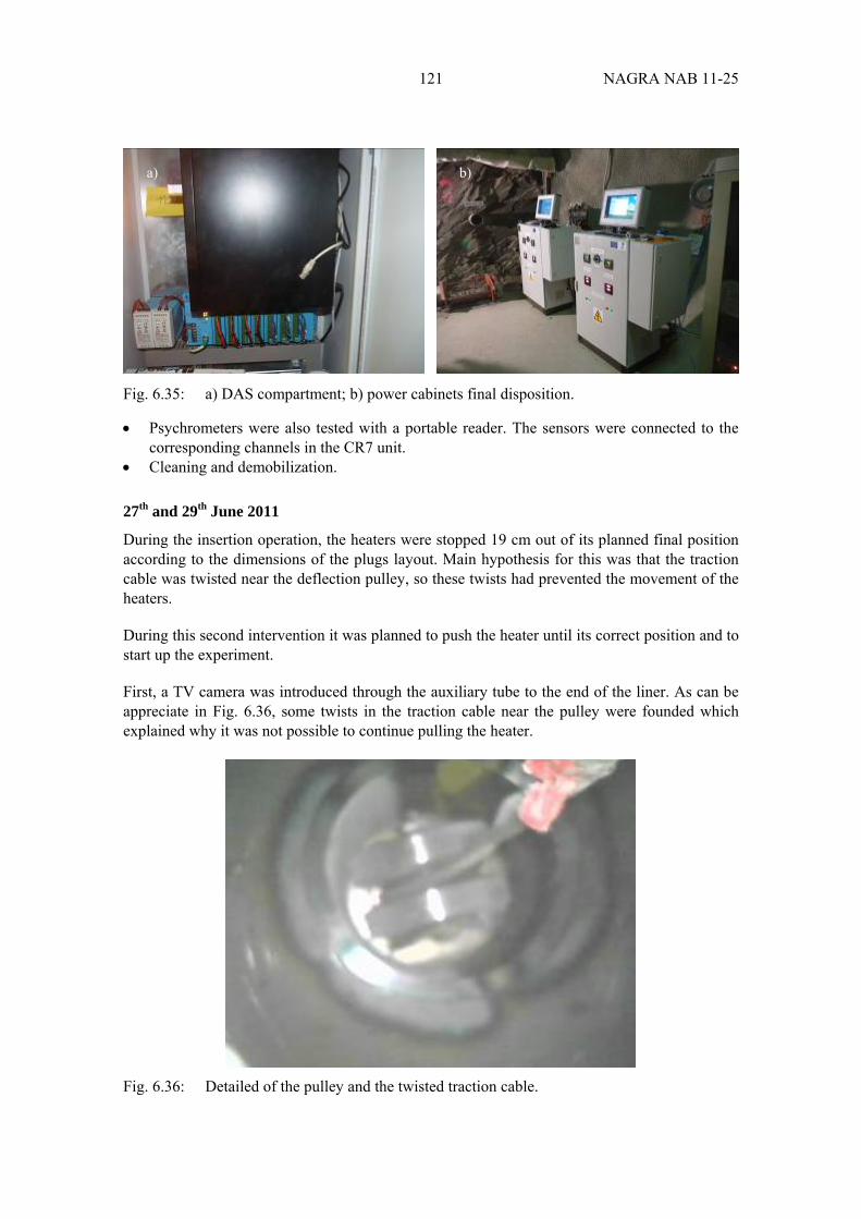
121 NAGRA NAB 11-25
Fig. 6.35: a) DAS compartment; b) power cabinets final disposition.
Psychrometers were also tested with a portable reader. The sensors were connected to the corresponding channels in the CR7 unit.
Cleaning and demobilization.
27th and 29th June 2011
During the insertion operation, the heaters were stopped 19 cm out of its planned final position according to the dimensions of the plugs layout. Main hypothesis for this was that the traction cable was twisted near the deflection pulley, so these twists had prevented the movement of the heaters.
During this second intervention it was planned to push the heater until its correct position and to start up the experiment.
First, a TV camera was introduced through the auxiliary tube to the end of the liner. As can be appreciate in Fig. 6.36, some twists in the traction cable near the pulley were founded which explained why it was not possible to continue pulling the heater.
Fig. 6.36: Detailed of the pulley and the twisted traction cable.
a) b)

NAGRA NAB 11-25 122
A hydraulic cylinder was then fixed to a column installed in front of the borehole entrance in order to push the heater to their final position. This operation moved the assembly 18 cm inside the liner (until its end).
After the repositioning of the heaters, several tests with the DAC and the power control system were made.
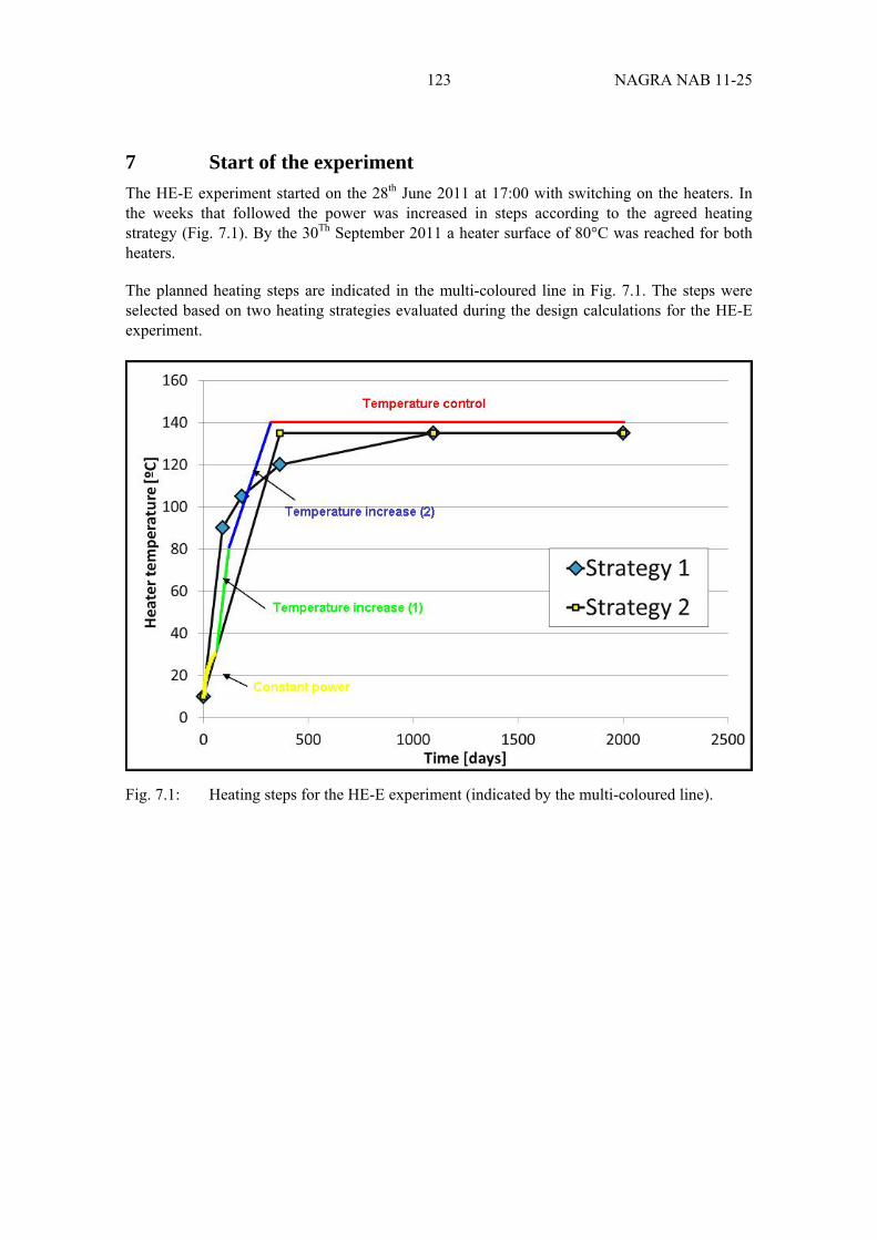
123 NAGRA NAB 11-25
7 Start of the experiment
The HE-E experiment started on the 28th June 2011 at 17:00 with switching on the heaters. In the weeks that followed the power was increased in steps according to the agreed heating strategy (Fig. 7.1). By the 30Th September 2011 a heater surface of 80°C was reached for both heaters.
The planned heating steps are indicated in the multi-coloured line in Fig. 7.1. The steps were selected based on two heating strategies evaluated during the design calculations for the HE-E experiment.
Fig. 7.1: Heating steps for the HE-E experiment (indicated by the multi-coloured line).

125 NAGRA NAB 11-25
8 References
Bossart P. and Steiger H. (2003). Ventilation (VE) Experiment: Borehole Inventory of Effectively Drilled BVE Boreholes, TECHNICAL NOTE 2003-11, IG St-Ursanne, December 2002
Fechner, T. (2001) SensInv2D-Manual, Geotomographie, Neuwied.
Flotron, HE-E Experiment: 3D Scanning of microtunnel VE with Tachymeter, TECHNICAL NOTE 2011-12, October 2010
Gaus I. (ed.): Long term Performance of Engineered Barrier Systems (PEBS) : Mont Terri HE-E experiment: detailed design. Nagra Arbeitsbericht NAB 11-01. Nagra, Wettingen, 2011.
Kemna, A. (1995): Tomographische Inversion des spezifischen Widerstandes in der Geoelektrik, Master Thesis, Universität Köln.
Mayor, J. C., García-Siñeriz, J. L., Velasco, M., Gómez- Hernández, J., Lloret, A., Matray, J.-M, Coste, F., Giraud, A., Rothfuchs, T., Marshall, P., Roesli, U. & Mayer, G. (2007): Ventilation Experiment in Opalinus Clay for the disposal of radioactive waste in underground repositories. – In: Bossart, P. & Nussbaum, C. (Eds.): Mont Terri Project – Heater Experiment, Engineered Barrier Emplacement and Ventilation Experiment (p.182–240). – Rep. Swiss Geol. Surv. 1.
Plötze M., Weber H.P (2007): ESDRED: Emplacement tests with granular bentonite MX-80: Laboratory results from ETH Zürich. Nagra Arbeitsbericht NAB 07-24. Nagra, Wettingen, 2007.
Rothfuchs, T., Hartwig, L., Hellwald, K., Komischke, M., Miehe, R., Wieczorek, K. (2004): Ventilation Test at Mont Terri: Geoelectric Monitoring of Opalinus Clay Desaturation, Gesellschaft für Anlagen- und Reaktorsicherheit mbH, GRS-207.
Schuster, K. (2007): High resolution seismic investigations within the VE-Experiment, Mont Terri Technical Report TR 07-06, swisstopo, Wabern, Switzerland.
Schuster, K. and Alheid H.-J. (2004): EB: Engineered Barrier Experiment; Seismic Long Term Observation in the EB Niche, Mont Terri Technical Report TR 04-02, swisstopo, Wabern, Switzerland.
Solexperts (2004,a): Ventilation Experiment in Opalinus Clay, “VE” Experiment, Data Acquisition System Report and Master Databases.
Solexperts (2004,b): Ventilation Experiment in Opalinus Clay, “VE” Experiment, Summary Data Report of the VE Master Databases (Period: July 2002 – June 2004).
Thury, M. & Bossart P., (1999). Mont Terri Rock Laboratory –results of the hydrogeological, geochemical and geotechnical experiments performed in 1996 and 1997 – Geol. Rep. Swiss natl. hydrol. Geol. Surv. 23.


Appendix 1 / A-1 NAGRA NAB 11-25
Appendix 1 Laboratory tests of bentonite blocks

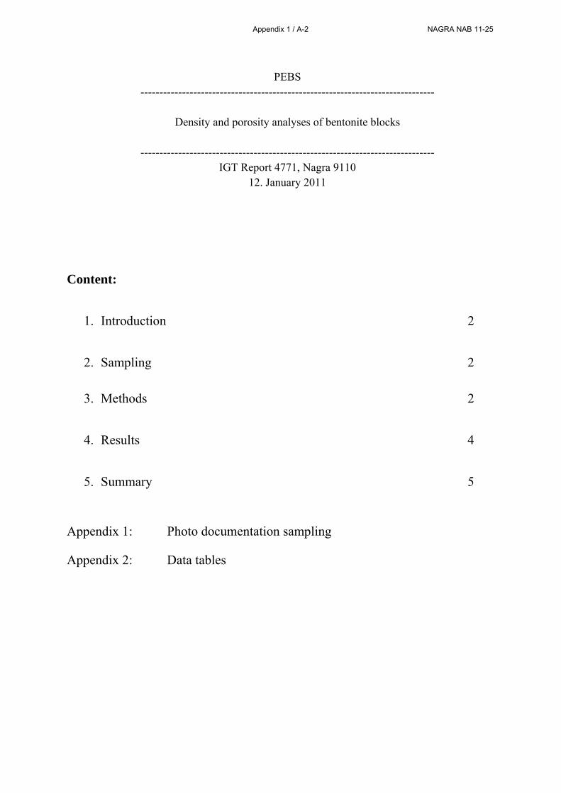
PEBS
------------------------------------------------------------------------------
Density and porosity analyses of bentonite blocks
------------------------------------------------------------------------------ IGT Report 4771, Nagra 9110
12. January 2011
Content:
1. Introduction 2
2. Sampling 2
3. Methods 2
4. Results 4
5. Summary 5
Appendix 1: Photo documentation sampling
Appendix 2: Data tables
Appendix 1 / A-2 NAGRA NAB 11-25
1 Introduction
The bentonite buffer construction around the canister in nuclear waste disposal involves a foundation of the canister made from highly compacted bentonite blocks. NAGRA assigned the Institute of Geotechnical Engineering of the ETH Zurich (IGT) with the analysis of a bentonite block made from MX-80 by Alpha Ceramics GmbH Germany from 23 November 2010 concerning density, water content and porosity and the homogeneity of these parameters within the block.
2 Sampling
The sealed block was delivered on 10 December. To investigate the homogeneity in compaction samples were taken from different localities of the block: Diagonal on opposite corners (E) and edges (K) (each 4 samples), from each face (S) (6 samples) and randomly in the middle (M) of the block (4 samples). Appendix 1 shows the photo documentation of the sampling
Appendix 1 / A-3 NAGRA NAB 11-25

3 Methods
3.1. Water content
The gravimetric water content (w) is defined as the ratio between the weight of water and the weight of dry solid expressed as a percentage. The water content was determined in accordance with SN 670 3406. Approx. 2 g material (moist) were weighed out immediately after sampling on 12 December 2010 and dried at 105 – 110 °C for 48 h.
w = water content in per cent, M = sample mass in moist state and Md = sample mass after drying.
From the gravimetric water content, the volumetric can be calculated as follows:
dv ww
w = gravimetric water content in per cent, wv = volumetric water content in per cent, ρd = dry bulk density of the material in g/cm3.
wM M
M100
d
d
Appendix 1 / A-4 NAGRA NAB 11-25
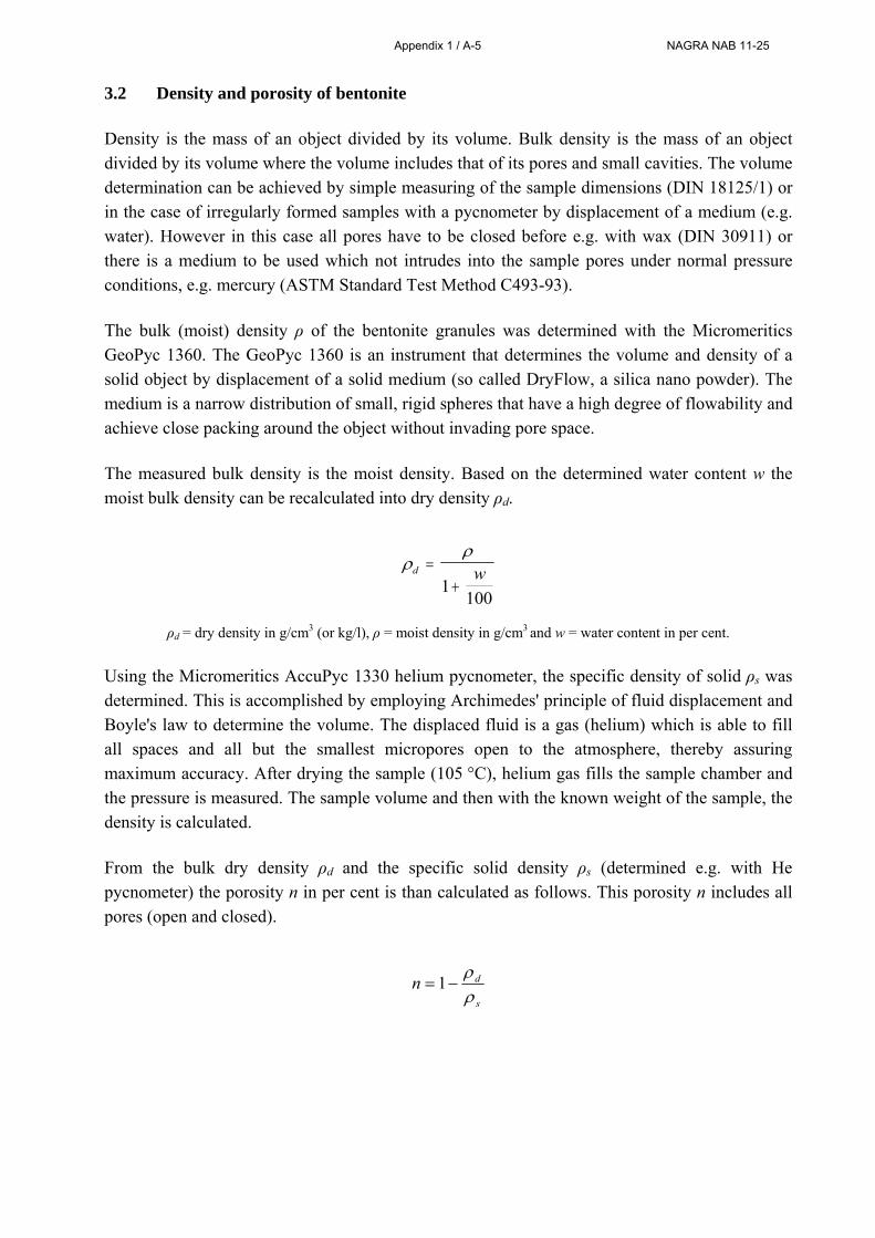
3.2 Density and porosity of bentonite
Density is the mass of an object divided by its volume. Bulk density is the mass of an object divided by its volume where the volume includes that of its pores and small cavities. The volume determination can be achieved by simple measuring of the sample dimensions (DIN 18125/1) or in the case of irregularly formed samples with a pycnometer by displacement of a medium (e.g. water). However in this case all pores have to be closed before e.g. with wax (DIN 30911) or there is a medium to be used which not intrudes into the sample pores under normal pressure conditions, e.g. mercury (ASTM Standard Test Method C493-93).
The bulk (moist) density ρ of the bentonite granules was determined with the Micromeritics GeoPyc 1360. The GeoPyc 1360 is an instrument that determines the volume and density of a solid object by displacement of a solid medium (so called DryFlow, a silica nano powder). The medium is a narrow distribution of small, rigid spheres that have a high degree of flowability and achieve close packing around the object without invading pore space.
The measured bulk density is the moist density. Based on the determined water content w the moist bulk density can be recalculated into dry density ρd.
ρd = dry density in g/cm3 (or kg/l), ρ = moist density in g/cm3 and w = water content in per cent.
Using the Micromeritics AccuPyc 1330 helium pycnometer, the specific density of solid ρs was determined. This is accomplished by employing Archimedes' principle of fluid displacement and Boyle's law to determine the volume. The displaced fluid is a gas (helium) which is able to fill all spaces and all but the smallest micropores open to the atmosphere, thereby assuring maximum accuracy. After drying the sample (105 °C), helium gas fills the sample chamber and the pressure is measured. The sample volume and then with the known weight of the sample, the density is calculated.
From the bulk dry density ρd and the specific solid density ρs (determined e.g. with He pycnometer) the porosity n in per cent is than calculated as follows. This porosity n includes all pores (open and closed).
s
dn
1
d 1
w
100
Appendix 1 / A-5 NAGRA NAB 11-25
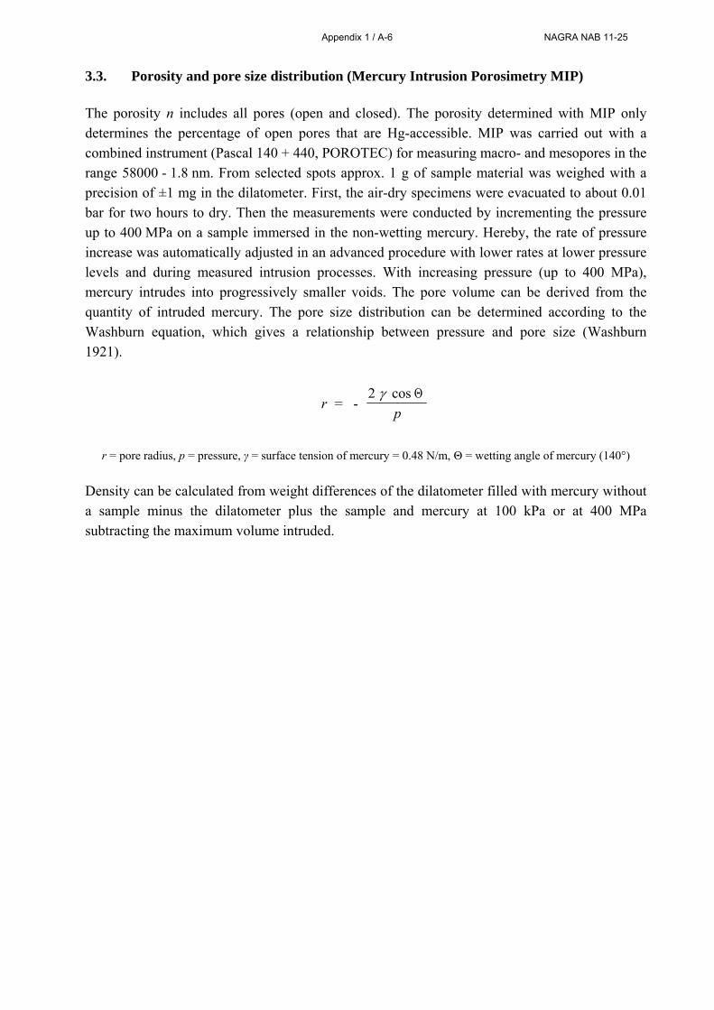
3.3. Porosity and pore size distribution (Mercury Intrusion Porosimetry MIP)
The porosity n includes all pores (open and closed). The porosity determined with MIP only determines the percentage of open pores that are Hg-accessible. MIP was carried out with a combined instrument (Pascal 140 + 440, POROTEC) for measuring macro- and mesopores in the range 58000 - 1.8 nm. From selected spots approx. 1 g of sample material was weighed with a precision of ±1 mg in the dilatometer. First, the air-dry specimens were evacuated to about 0.01 bar for two hours to dry. Then the measurements were conducted by incrementing the pressure up to 400 MPa on a sample immersed in the non-wetting mercury. Hereby, the rate of pressure increase was automatically adjusted in an advanced procedure with lower rates at lower pressure levels and during measured intrusion processes. With increasing pressure (up to 400 MPa), mercury intrudes into progressively smaller voids. The pore volume can be derived from the quantity of intruded mercury. The pore size distribution can be determined according to the Washburn equation, which gives a relationship between pressure and pore size (Washburn 1921).
r = pore radius, p = pressure, γ = surface tension of mercury = 0.48 N/m, Θ = wetting angle of mercury (140°)
Density can be calculated from weight differences of the dilatometer filled with mercury without a sample minus the dilatometer plus the sample and mercury at 100 kPa or at 400 MPa subtracting the maximum volume intruded.
rp
= - 2 cos
Appendix 1 / A-6 NAGRA NAB 11-25
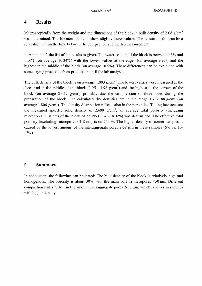
4 Results
Macroscopically from the weight and the dimensions of the block, a bulk density of 2.08 g/cm3 was determined. The lab measurements show slightly lower values. The reason for this can be a relaxation within the time between the compaction and the lab measurement.
In Appendix 2 the list of the results is given. The water content of the block is between 9.3% and 11.6% (on average 10.34%) with the lowest values at the edges (on average 9.9%) and the highest in the middle of the block (on average 10.9%). These differences can be explained with some drying processes from production until the lab analysis.
The bulk density of the block is on average 1.993 g/cm3. The lowest values were measured at the faces and in the middle of the block (1.95 - 1.98 g/cm3) and the highest at the corners of the block (on average 2.059 g/cm3) probably due the compression of three sides during the preparation of the block. The calculated dry densities are in the range 1.73-1.88 g/cm3 (on average 1.806 g/cm3). The density distribution reflects also in the porosities. Taking into account the measured specific solid density of 2.699 g/cm3, an average total porosity (including micropores <1.8 nm) of the block of 33.1% (30.4 – 36.0%) was determined. The effective total porosity (excluding micropores <1.8 nm) is on 24.4%. The higher density of corner samples is caused by the lowest amount of the interaggregate pores 2-58 µm in these samples (6% vs. 10-17%).
5 Summary
In conclusion, the following can be stated: The bulk density of the block is relatively high and homogenous. The porosity is about 30% with the main part in mesopores <50 nm. Different compaction states reflect in the amount interaggregate pores 2-58 µm, which is lower in samples with higher density.
Appendix 1 / A-7 NAGRA NAB 11-25
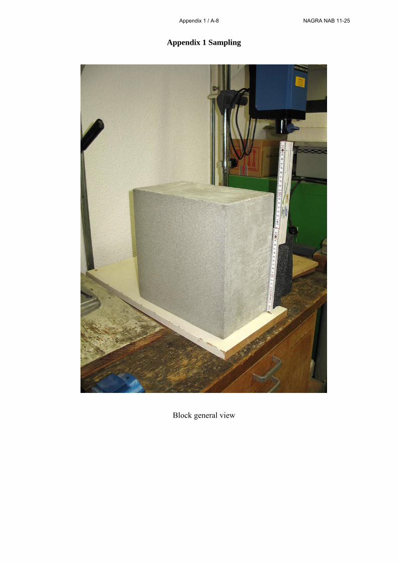
Appendix 1 Sampling
Block general view
Appendix 1 / A-8 NAGRA NAB 11-25
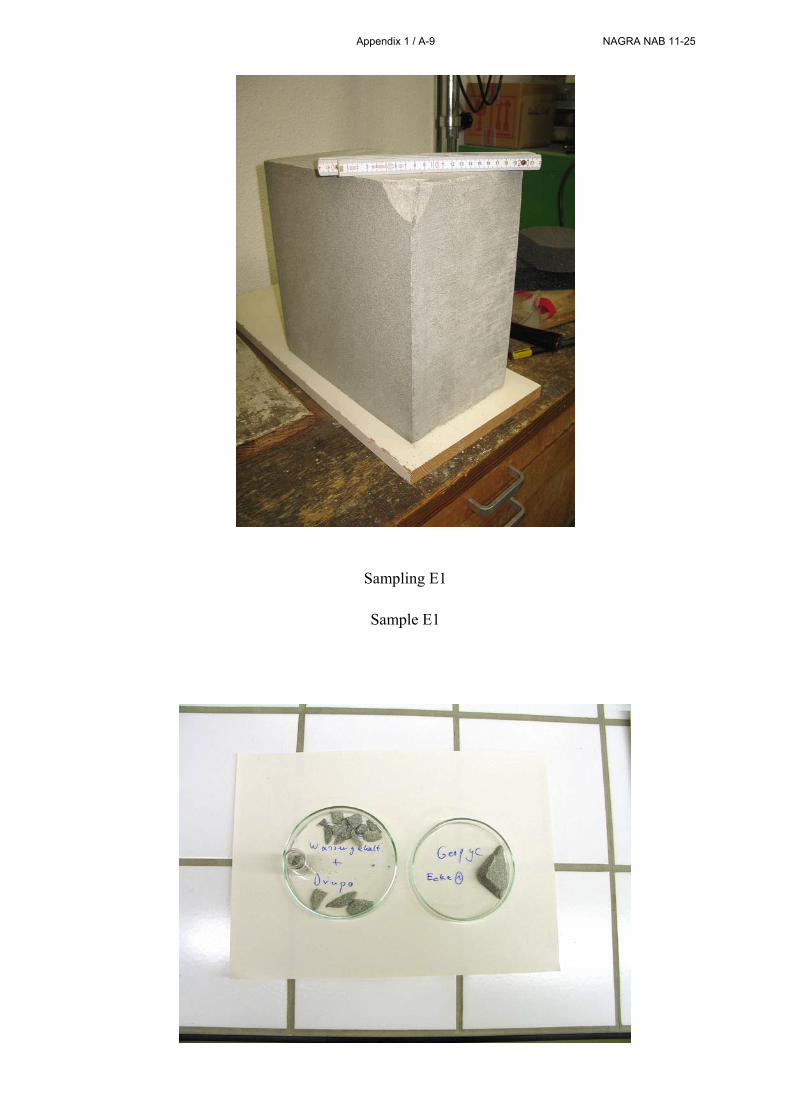
Sampling E1
Sample E1
Appendix 1 / A-9 NAGRA NAB 11-25

Sampling K1
Sample K1
Appendix 1 / A-10 NAGRA NAB 11-25
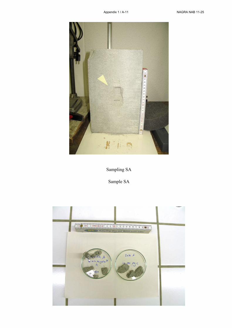
Sampling SA
Sample SA
Appendix 1 / A-11 NAGRA NAB 11-25
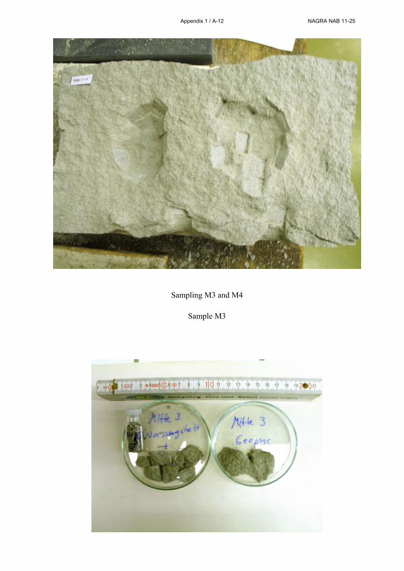
Sampling M3 and M4
Sample M3
Appendix 1 / A-12 NAGRA NAB 11-25
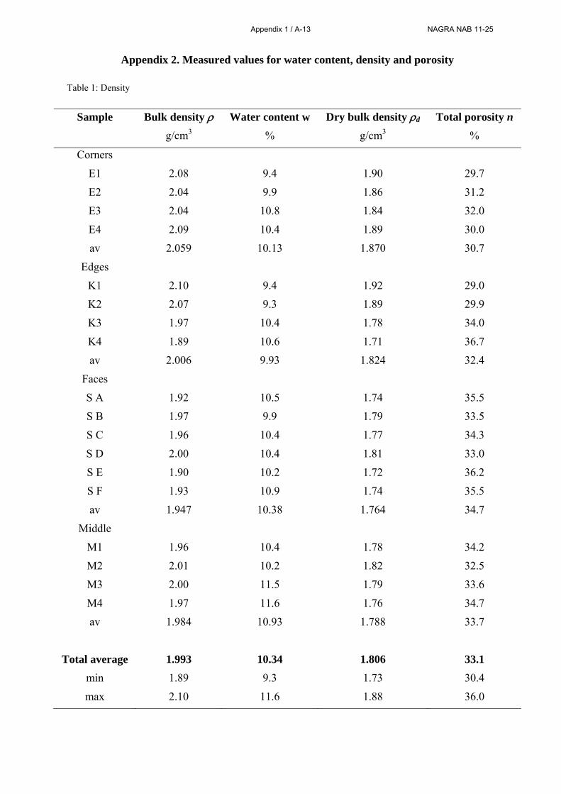
Appendix 2. Measured values for water content, density and porosity
Table 1: Density
Sample Bulk density Water content w Dry bulk density d Total porosity n
g/cm3 % g/cm3 %
Corners
E1 2.08 9.4 1.90 29.7
E2 2.04 9.9 1.86 31.2
E3 2.04 10.8 1.84 32.0
E4 2.09 10.4 1.89 30.0
av 2.059 10.13 1.870 30.7
Edges
K1 2.10 9.4 1.92 29.0
K2 2.07 9.3 1.89 29.9
K3 1.97 10.4 1.78 34.0
K4 1.89 10.6 1.71 36.7
av 2.006 9.93 1.824 32.4
Faces
S A 1.92 10.5 1.74 35.5
S B 1.97 9.9 1.79 33.5
S C 1.96 10.4 1.77 34.3
S D 2.00 10.4 1.81 33.0
S E 1.90 10.2 1.72 36.2
S F 1.93 10.9 1.74 35.5
av 1.947 10.38 1.764 34.7
Middle
M1 1.96 10.4 1.78 34.2
M2 2.01 10.2 1.82 32.5
M3 2.00 11.5 1.79 33.6
M4 1.97 11.6 1.76 34.7
av 1.984 10.93 1.788 33.7
Total average 1.993 10.34 1.806 33.1
min 1.89 9.3 1.73 30.4
max 2.10 11.6 1.88 36.0
Appendix 1 / A-13 NAGRA NAB 11-25
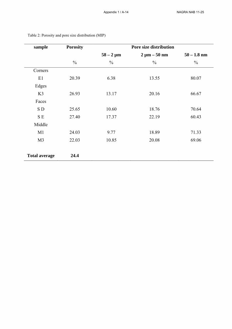
Table 2: Porosity and pore size distribution (MIP)
sample Porosity Pore size distribution
58 – 2 µm 2 µm – 50 nm 50 – 1.8 nm
% % % %
Corners
E1 20.39 6.38 13.55 80.07
Edges
K3 26.93 13.17 20.16 66.67
Faces
S D 25.65 10.60 18.76 70.64
S E 27.40 17.37 22.19 60.43
Middle
M1 24.03 9.77 18.89 71.33
M3 22.03 10.85 20.08 69.06
Total average 24.4
Appendix 1 / A-14 NAGRA NAB 11-25

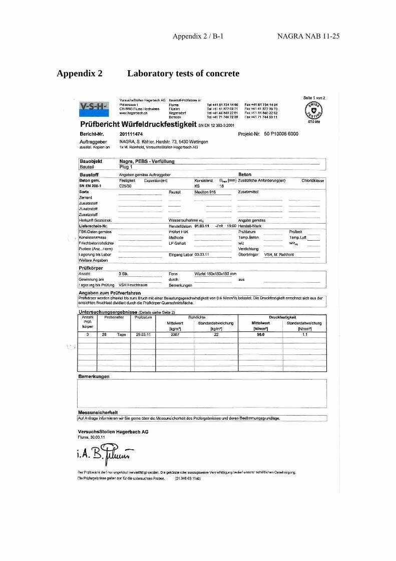
Appendix 2 / B-1 NAGRA NAB 11-25
Appendix 2 Laboratory tests of concrete
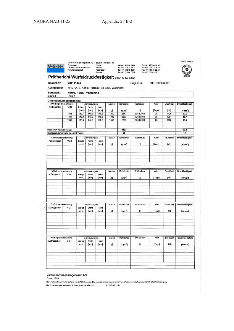
NAGRA NAB 11-25 Appendix 2 / B-2

Appendix 3 / C-1 NAGRA NAB 11-25
Appendix 3 Coordinates of all sensors
Tab. A.3.1: List of sensors for the HE-E experiment, including the type of sensors, the distance to the tunnel surface or centre of the tunnel and location in PEBS coordinate system

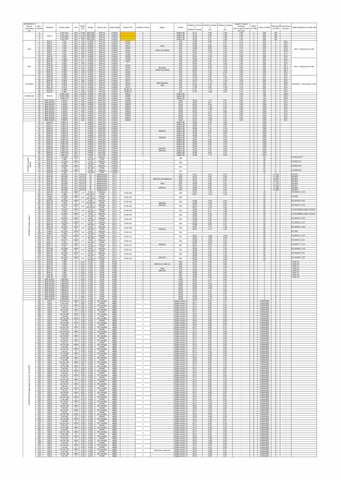
INTERFACE/Sensor
assembling box
DAS - Channel
Borehole Sensor name UnitDepth
[m]Range Sensor type Output signal Sensor SN Number of wires Status Profile
Position of sensorZ
[PEBS m tunnel]
Position of sensorX
[m]
Position of sensorY
[m]
Height P-Sensor membran
above casted tunnel floor (m)
Offset on GMII
Factor on GMIIReference on GMII
Atmos-pheric pressure
Cable identification at DAS side
1 P-B1-13m kPa 13.00 100-2100 PAA-23 4-20mA 2 Gallery 98 31.37 0.28 -2.04 1.50 -1 500 1002 P-B1-11m kPa 11.00 100-2100 PAA-23 4-20mA 2 Gallery 98 31.32 2.28 -1.86 1.50 -1 500 1003 P-B1-09m kPa 9.00 100-2100 PAA-23 4-20mA 2 Gallery 98 31.26 4.27 -1.68 1.25 -1 500 1004 P-B1-07m kPa 7.00 100-2100 PAA-23 4-20mA 2 Gallery 98 31.20 6.22 -1.50 1.25 -1 500 1005 BVE-2 P-B2 kPa 1.55 0-2000 PAA-23 4-20mA 42183 2 SA4 33.88 0.00 2.30 0.70 -1 500 0 88.26 BVE-3 P-B3 kPa 1.04 0-2000 PAA-23 4-20mA 42194 2 SA4 34.98 1.17 1.76 0.70 -1 500 0 92.87 BVE-4 P-B4 kPa 1.05 0-2000 PAA-23 4-20mA 42172 2 noisy SA4 34.98 1.68 0.25 0.70 -1 500 0 102.28 BVE-5 P-B5 kPa 0.55 0-2000 PAA-23 4-20mA 42180 2 SA4 34.98 0.85 -0.31 0.70 -1 500 0 92.69 BVE-6 P-B6 kPa 1.63 0-2000 PAA-23 4-20mA 42181 2 reacts very slowly SA4 36.13 -0.02 -1.26 0.35 -1 500 0 119.010 BVE-7 P-B7 kPa 2.06 0-2000 PAA-23 4-20mA 42182 2 SA4 34.97 -1.94 -1.36 0.35 -1 500 0 97.311 BVE-8 P-B8 kPa 0.50 0-2000 PAA-23 4-20mA 42188 2 SA4 34.97 -1.15 0.36 0.35 -1 500 0 92.212 BVE-9 P-B9 kPa 1.40 0-2000 PAA-23 4-20mA 42196 2 SA4 34.97 -1.43 2.02 0.35 -1 500 0 92.413 BVE-55 P-B55 kPa 2.11 0-2000 PAA-23 4-20mA 42169 2 SA2 29.63 -0.01 3.39 0.30 -1 500 0 94.314 BVE-56 P-B56 kPa 2.11 0-2000 PAA-23 4-20mA 42167 2 SA2 29.64 1.94 2.44 0.30 -1 500 0 93.715 BVE-57 P-B57 kPa 1.80 0-2000 PAA-23 4-20mA ? 2 SA2 29.64 2.31 -0.36 0.30 -1 500 0 97.916 BVE-58 P-B58 kPa 1.12 0-2000 PAA-23 4-20mA 42184 2 SA2 29.63 1.28 -0.75 0.30 -1 500 0 98.117 BVE-59 P-B59 kPa 2.12 0-2000 PAA-23 4-20mA 42193 2 Bad data SA2 29.63 -0.01 -2.30 0.65 -1 500 0 101.218 BVE-60 P-B60 kPa 1.50 0-2000 PAA-23 4-20mA 42170 2 reacts very slowly SA2 29.62 -1.54 -1.03 0.65 -1 500 0 95.319 BVE-61 P-B61 kPa 1.80 0-2000 PAA-23 4-20mA 42185 2 SA2 29.61 -2.31 -0.36 0.65 -1 500 0 95.320 BVE-62 P-B62 kPa 2.13 0-2000 PAA-23 4-20mA 42195 2 SA2 29.62 -1.94 2.47 0.65 -1 500 0 93.521 BVE-38 P-B38 kPa 2.10 0-2000 PAA-23 4-20mA 42191 2 SA3 31.49 1.94 2.46 0.35 -1 500 0 93.522 BVE-39 P-B39 kPa 2.11 0-2000 PAA-23 4-20mA 42176 2 SA3 31.49 1.92 -1.49 0.35 -1 500 0 93.523 BVE-40 P-B40 kPa 1.80 0-2000 PAA-23 4-20mA 42177 2 SA3 31.47 -1.73 -1.24 0.35 -1 500 0 95.224 BVE-41 P-B41 kPa 1.81 0-2000 PAA-23 4-20mA 42187 2 often bad data SA3 31.47 -1.74 2.25 0.35 -1 500 0 98.825 BVE-78 P-B78 kPa 2.10 0-2000 PAA-23 4-20mA 42173 2 noisy SA1 27.99 1.95 2.39 0.70 -1 500 0 93.626 BVE-79 P-B79 kPa 2.10 0-2000 PAA-23 4-20mA 42175 2 SA1 27.99 1.95 -1.49 0.70 -1 500 0 84.627 BVE-80 P-B80 kPa 1.81 0-2000 PAA-23 4-20mA 42192 (?) 2 SA1 27.97 -1.76 -1.28 0.70 -1 500 0 96.128 BVE-81 P-B81 kPa 1.80 0-2000 PAA-23 4-20mA 42189 (?) 2 SA1 27.97 -1.86 2.06 0.70 -1 500 0 93.629 P-B91-10m kPa 10.00 0-3000 PAA-33X 4-20mA 65014 2 Gallery 98 1.05 -1 750 0 108.330 P-B91-08m kPa 8.82 0-3000 PAA-33X 4-20mA 65269 2 Gallery 98 1.05 -1 750 0 100.231 P-B91-07m kPa 7.66 0-3000 PAA-33X 4-20mA 47458 2 Gallery 98 1.05 -1 750 0 109.432 BHE-ESA21 P-BA21 kPa 0.60 0-5000 PAA-23X 4-20mA 146519 2 SA20 29.62 1.14 0.91 0.80 -1 1250 0 92.433 BHE-ESA22 P-BA22 kPa 1.00 0-5000 PAA-23X 4-20mA 146520 2 SA20 29.62 0.57 2.01 0.80 -1 1250 0 92.034 BHE-ESA23 P-BA23 kPa 0.60 0-5000 PAA-23X 4-20mA 146521 2 SA20 29.62 -0.51 1.72 0.50 -1 1250 0 92.035 BHE-ESA24 P-BA24 kPa 1.00 0-5000 PAA-23X 4-20mA 146522 2 SA20 29.62 -1.58 1.03 0.50 -1 1250 0 92.036 BHE-ESA25 P-BA25 kPa 0.30 0-5000 PAA-23X 4-20mA 146523 2 SA20 29.62 -0.98 0.47 0.50 -1 1250 0 92.037 BHE-ESD21 P-BD21 kPa 0.60 0-5000 PAA-23X 4-20mA 146514 2 SD20 33.32 1.24 0.96 0.80 -1 1250 0 92.938 BHE-ESD22 P-BD22 kPa 1.00 0-5000 PAA-23X 4-20mA 146515 2 SD20 33.32 0.62 2.05 0.80 -1 1250 0 92.939 BHE-ESD23 P-BD23 kPa 0.60 0-5000 PAA-23X 4-20mA 146516 2 SD20 33.32 -0.45 1.81 0.50 -1 1250 0 92.540 BHE-ESD24 P-BD24 kPa 1.00 0-5000 PAA-23X 4-20mA 146517 2 SD20 33.32 -1.56 1.20 0.50 -1 1250 0 92.041 BHE-ESD25 P-BD25 kPa 0.30 0-5000 PAA-23X 4-20mA 146518 2 SD20 33.32 -0.70 1.35 0.50 -1 1250 0 90.142 BHE-E1 P-BE1-I1 kPa 0-5000 PAA-23X 4-20mA 2 Gallery 98 28.98 4.26 -0.46 -1 1250 043 BHE-E1 P-BE1-I2 kPa 0-5000 PAA-23X 4-20mA 2 Gallery 98 28.98 5.07 -0.55 -1 1250 044 BHE-E1 P-BE1-I3 kPa 0-5000 PAA-23X 4-20mA 2 Gallery 98 28.98 6.17 -0.67 -1 1250 045 BHE-E1 P-BE1-I4 kPa 0-5000 PAA-23X 4-20mA 2 Gallery 98 28.98 7.27 -0.79 -1 1250 046 BHE-E2 P-BE2-I1 kPa 0-5000 PAA-23X 4-20mA 2 defective Gallery 98 33.98 4.26 -0.46 -1 1250 047 BHE-E2 P-BE2-I2 kPa 0-5000 PAA-23X 4-20mA 2 Gallery 98 33.98 5.07 -0.55 -1 1250 048 BHE-E2 P-BE2-I3 kPa 0-5000 PAA-23X 4-20mA 2 Gallery 98 33.98 6.17 -0.67 -1 1250 049 BHE-E2 P-BE2-I4 kPa 0-5000 PAA-23X 4-20mA 2 defective Gallery 98 33.98 7.27 -0.79 -1 1250 050 BHE-E1 P-BE1-P1 kPa 0-5000 PAA-23X 4-20mA 2 Gallery 98 28.98 4.61 -0.50 -1 1250 051 BHE-E1 P-BE1-P2 kPa 0-5000 PAA-23X 4-20mA 2 Gallery 98 28.98 5.52 -0.60 -1 1250 052 BHE-E1 P-BE1-P3 kPa 0-5000 PAA-23X 4-20mA 2 Gallery 98 28.98 6.82 -0.74 -1 1250 053 BHE-E1 P-BE1-P4 kPa 0-5000 PAA-23X 4-20mA 2 Gallery 98 28.98 7.73 -0.84 -1 1250 054 BHE-E2 P-BE2-P1 kPa 0-5000 PAA-23X 4-20mA 2 defective Gallery 98 33.98 4.61 -0.50 -1 1250 055 BHE-E2 P-BE2-P2 kPa 0-5000 PAA-23X 4-20mA 2 defective Gallery 98 33.98 5.52 -0.60 -1 1250 056 BHE-E2 P-BE2-P3 kPa 0-5000 PAA-23X 4-20mA 2 Gallery 98 33.98 6.82 -0.74 -1 1250 057 BHE-E2 P-BE2-P4 kPa 0-5000 PAA-23X 4-20mA 2 Gallery 98 33.98 7.73 -0.84 -1 1250 065 BVE-95 HC-B95 %RH 0-100 Rotronic 4-20mA - -1 25 0 - HC-B91 (22) **66 BVE-95 T-B95 °C -40-180 Pt100 4-20mA - -1 25 0 -67 BVE-92 HC-B92 %RH 0-100 Rotronic 4-20mA - -1 25 0 - HC-B92 (17)68 BVE-92 T-B92 °C -40-180 Pt100 4-20mA - -1 25 0 -69 BVE-94 HC-B94 %RH 0-100 Rotronic 4-20mA - -1 25 0 - HC-B94 (07)70 BVE-94 T-B94 °C -40-180 Pt100 4-20mA - -1 25 0 -71 BVE-93 HC-B93 %RH 0-100 Rotronic 4-20mA - -1 25 0 - HC-B93 (12)72 BVE-93 T-B93 °C -40-180 Pt100 4-20mA - -1 25 0 -73 BVE-25 RD-B25 mm 0.0-2.0 25 displacement 0-5 V - 3 SD2 33.33 -0.01 3.23 - 0 5 -17.490 - RD-B2574 BVE-26 RD-B26 mm 0.0-2.0 25 displacement 0-5 V - 3 SD2 33.34 2.62 0.08 - 0 5 -17.394 - RD-B2675 BVE-27 RD-B27 mm 0.0-2.0 25 displacement 0-5 V - 3 defective and displaced SD2 33.33 -0.01 -2.13 - 0 5 -19.405 - RD-B2776 BVE-28 RD-B28 mm 0.0-2.0 25 displacement 0-5 V - 3 SD2 33.31 -2.61 0.07 - 0 5 -17.911 - RD-B2877 BVE-46 RD-B46 mm 0.0-2.0 25 displacement 0-5 V - 3 noisy SD1 30.88 0.00 3.22 - 0 5 -17.710 - RD-B4678 BVE-47 RD-B47 mm 0.0-2.0 25 displacement 0-5 V - 3 SD1 30.89 2.62 0.04 - 0 5 -17.362 - RD-B4779 BVE-48 RD-B48 mm 0.0-2.0 25 displacement 0-5 V - 3 defective SD1 30.88 0.00 -2.16 - 0 5 -17.592 - RD-B4880 BVE-49 RD-B49 mm 0.0-2.0 25 displacement 0-5 V - 3 SD1 30.86 -2.61 0.04 - 0 5 -17.580 - RD-B4981 BVE-20 HC-B20 %RH 0-100 Rotronic 0-5 V 33.97 -1.24 -0.21 - 0 20 0 - HC BVE20 / 0.7882 BVE-20 T-B20 °C -40-180°C Pt100 0-5 V 33.97 -1.24 -0.21 - 0 20 0 -83 surface HC-SB2 %RH 0-100 Rotronic 0-5 V - 0 20 0 - HC SB284 surface T-SB2 °C -40-180°C Pt100 0-5 V - 0 20 0 -85 BVE-18 HC-B18 %RH 0-100 Rotronic 0-5 V 33.98 -0.34 -0.41 - 0 20 0 - HC BVE18 / 0.3586 BVE-18 T-B18 °C -40-180°C Pt100 0-5 V bad data 33.98 -0.34 -0.41 - 0 20 0 -87 BVE-75 HC-B75 %RH 0-100 Rotronic 0-5 V defective 28.97 -1.02 1.05 - 0 20 0 - HC BVE75 / 0.5288 BVE-75 T-B75 °C -40-180°C Pt100 0-5 V 28.97 -1.02 1.05 - 0 20 0 -89 BVE-16 HC-B16 %RH 0-100 Rotronic 0-5 V 33.98 0.71 -1.50 - 0 20 0 - not identifiable (cable in beton)90 BVE-16 T-B16 °C -40-180 Pt100 0-5 V 33.98 0.71 -1.50 - 0 20 0 -91 BVE-12 HC-B12 %RH 0-100 Rotronic 0-5 V 33.99 1.59 1.48 - 0 20 0 - not identifiable (cable in beton)92 BVE-12 T-B12 °C -40-180 Pt100 0-5 V 33.99 1.59 1.48 - 0 20 0 -93 BVE-14 HC-B14 %RH 0-100 Rotronic 0-5 V 33.98 1.02 -0.07 - 0 20 0 - HC BVE14 / 0.5394 BVE-14 T-B14 °C -40-180 Pt100 0-5 V 33.98 1.02 -0.07 - 0 20 0 -95 BVE-10 HC-B10 %RH 0-100 Rotronic 0-5 V 33.98 0.25 1.41 - 0 20 0 - HC BVE10 / 0.2796 BVE-10 T-B10 °C -40-180 Pt100 0-5 V 33.98 0.25 1.41 - 0 20 0 -97 BVE-23 HC-B23 %RH 0-100 Rotronic 0-5 V 33.97 -1.47 1.39 - 0 20 0 - HC BVE23 / 1.0598 BVE-23 T-B23 °C -40-180 Pt100 0-5 V defective 33.97 -1.47 1.39 - 0 20 0 -99 surface HC-SB1 %RH 0-100 Rotronic 0-5 V - 0 20 0 - HC SB1100 surface T-SB1 °C -40-180 Pt100 0-5 V - 0 20 0 -101 BVE-73 HC-B73 %RH 0-100 Rotronic 0-5 V 28.97 -1.65 -0.49 - 0 20 0 - HC BVE73 / 1.25102 BVE-73 T-B73 °C -40-180 Pt100 0-5 V 28.97 -1.65 -0.49 - 0 20 0 -103 BVE-71 HC-B71 %RH 0-100 Rotronic 0-5 V 28.98 -0.30 -0.41 - 0 20 0 - HC BVE71 / 0.27104 BVE-71 T-B71 °C -40-180 Pt100 0-5 V 28.98 -0.30 -0.41 - 0 20 0 -105 BVE-77 HC-B77 %RH 0-100 Rotronic 0-5 V defective 28.97 -0.67 2.55 - 0 20 0 - HC BVE77 / 1.54106 BVE-77 T-B77 °C -40-180 Pt100 0-5 V 28.97 -0.67 2.55 - 0 20 0 -107 BVE-66 HC-B66 %RH 0-100 Rotronic 0-5 V 28.98 1.24 1.18 - 0 20 0 - HC BVE66 / 0.78108 BVE-66 T-B66 °C -40-180 Pt100 0-5 V 28.98 1.24 1.18 - 0 20 0 -109 BVE-64 HC-B64 %RH 0-100 Rotronic 0-5 V 28.98 0.40 1.39 - 0 20 0 - HC BVE64 / 0.37110 BVE-64 T-B64 °C -40-180 Pt100 0-5 V 28.98 0.40 1.39 - 0 20 0 -111 BVE-69 HC-B69 %RH 0-100 Rotronic 0-5 V defective 28.98 1.45 -0.38 - 0 20 0 - HC BVE69 / 1.02112 BVE-69 T-B69 °C -40-180 Pt100 0-5 V 28.98 1.45 -0.38 - 0 20 0 -121 BVE-25 T-B25 °C 0.10 0-100 Pt100 Pt100 - 4 SD2 33.33 -0.01 3.23 - 0 1 0 - T BVE 25122 BVE-26 T-B26 °C 0.10 0-100 Pt100 Pt100 - 4 defective & cable cut SD2 33.34 2.62 0.08 - 0 1 0 - T BVE 26123 BVE-27 T-B27 °C 0.10 0-100 Pt100 Pt100 - 4 SD2 33.33 -0.01 -2.13 - 0 1 0 - T BVE 27124 BVE-28 T-B28 °C 0.10 0-100 Pt100 Pt100 - 4 noisy SD2 33.31 -2.61 0.07 - 0 1 0 - T BVE 28125 BVE-46 T-B46 °C 0.10 0-100 Pt100 Pt100 - 4 defective SD1 30.88 0.00 3.22 - 0 1 0 - T BVE 46126 BVE-47 T-B47 °C 0.10 0-100 Pt100 Pt100 - 4 SD1 30.89 2.62 0.04 - 0 1 0 - T BVE 47127 BVE-48 T-B48 °C 0.10 0-100 Pt100 Pt100 - 4 SD1 30.88 0.00 -2.16 - 0 1 0 - T BVE 48128 BVE-49 T-B49 °C 0.10 0-100 Pt100 Pt100 - 4 SD1 30.86 -2.61 0.04 - 0 1 0 - T BVE 49129 BHE-ESA21 T-BESA21 °C 0.40 0-100 Pt100 Pt100 - 4 SA20 29.62 1.14 0.91 - 0 1 0 -130 BHE-ESA22 T-BESA22 °C 0.80 0-100 Pt100 Pt100 - 4 SA20 29.62 0.57 2.01 - 0 1 0 -131 BHE-ESA23 T-BESA23 °C 0.40 0-100 Pt100 Pt100 - 4 SA20 29.62 -0.51 1.72 - 0 1 0 -132 BHE-ESA24 T-BESA24 °C 0.80 0-100 Pt100 Pt100 - 4 SA20 29.62 -1.58 1.03 - 0 1 0 -133 BHE-ESA25 T-BESA25 °C 0.10 0-100 Pt100 Pt100 - 4 SA20 29.62 -0.98 0.47 - 0 1 0 -134 BHE-ESD21 T-BESD21 °C 0.40 0-100 Pt100 Pt100 - 4 SD20 33.32 1.24 0.96 - 0 1 0 -135 BHE-ESD22 T-BESD22 °C 0.80 0-100 Pt100 Pt100 - 4 SD20 33.32 0.62 2.05 - 0 1 0 -136 BHE-ESD23 T-BESD23 °C 0.40 0-100 Pt100 Pt100 - 4 SD20 33.32 -0.45 1.81 - 0 1 0 -137 BHE-ESD24 T-BESD24 °C 0.80 0-100 Pt100 Pt100 - 4 SD20 33.32 -1.56 1.20 - 0 1 0 -138 BHE-ESD25 T-BESD25 °C 0.10 0-100 Pt100 Pt100 - 4 SD20 33.32 -0.70 1.35 - 0 1 0 -202 NSC3 HC-N3-12H %RH 0.00 0-100 IST humidity digital - Nagra carrier 3 32.77 0.00 1.17 - 0 0.00530555 0 -203 NSC3 T-N3-12H °C 0.00 0-165 Pt1000 digital - Nagra carrier 3 32.77 0.00 1.17 - 0 0.00351800 0 -204 NSC3 HC-N3-3H %RH 0.00 0-100 IST humidity digital - Nagra carrier 3 32.77 0.66 0.49 - 0 0.00530555 0 -205 NSC3 T-N3-3H °C 0.00 0-165 Pt1000 digital - Nagra carrier 3 32.77 0.66 0.49 - 0 0.00351800 0 -206 NSC3 HC-N3-9H %RH 0.00 0-100 IST humidity digital - Nagra carrier 3 32.77 0.64 0.49 - 0 0.00530555 0 -207 NSC3 T-N3-9H °C 0.00 0-165 Pt1000 digital - Nagra carrier 3 32.77 0.64 0.49 - 0 0.00351800 0 -208 NSC3 HC-N3-5Bt %RH -0.35 0-100 IST humidity digital - Nagra carrier 3 33.07 0.08 0.28 - 0 0.00530555 0 -209 NSC3 T-N3-5Bt °C -0.35 0-165 Pt1000 digital - Nagra carrier 3 33.07 0.08 0.28 - 0 0.00351800 0 -210 NSC2 HC-N2-5Bl %RH -0.20 0-100 IST humidity digital - Nagra carrier 2 34.07 0.08 0.20 - 0 0.00530555 0 -211 NSC2 T-N2-5Bl °C -0.20 0-165 Pt1000 digital - Nagra carrier 2 34.07 0.08 0.20 - 0 0.00351800 0 -212 NSC2 HC-N2-5Bt %RH -0.35 0-100 IST humidity digital - Nagra carrier 2 34.07 0.08 0.30 - 0 0.00530555 0 -213 NSC2 T-N2-5Bt °C -0.35 0-165 Pt1000 digital - Nagra carrier 2 34.07 0.08 0.30 - 0 0.00351800 0 -214 NSC3 HC-N3-12C %RH -0.35 0-100 IST humidity digital - Nagra carrier 3 32.77 0.00 0.74 - 0 0.00530555 0 -215 NSC3 T-N3-12C °C -0.35 0-165 Pt1000 digital - Nagra carrier 3 32.77 0.00 0.74 - 0 0.00351800 0 -216 NSC3 HC-N3-12M %RH -0.20 0-100 IST humidity digital - Nagra carrier 3 32.77 0.00 0.89 - 0 0.00530555 0 -217 NSC3 T-N3-12M °C -0.20 0-165 Pt1000 digital - Nagra carrier 3 32.77 0.00 0.89 - 0 0.00351800 0 -218 NSC3 HC-N3-3M %RH -0.20 0-100 IST humidity digital - Nagra carrier 3 32.77 0.40 0.49 - 0 0.00530555 0 -219 NSC3 T-N3-3M °C -0.20 0-165 Pt1000 digital - Nagra carrier 3 32.77 0.40 0.49 - 0 0.00351800 0 -220 NSC3 HC-N3-3C %RH -0.35 0-100 IST humidity digital - Nagra carrier 3 32.77 0.25 0.49 - 0 0.00530555 0 -221 NSC3 T-N3-3C °C -0.35 0-165 Pt1000 digital - Nagra carrier 3 32.77 0.25 0.49 - 0 0.00351800 0 -222 NSC1 HC-N1-3M %RH -0.20 0-100 IST humidity digital - Nagra carrier 1 34.77 0.40 0.53 - 0 0.00530555 0 -223 NSC1 T-N1-3M °C -0.20 0-165 Pt1000 digital - Nagra carrier 1 34.77 0.40 0.53 - 0 0.00351800 0 -224 NSC1 HC-N1-3C %RH -0.35 0-100 IST humidity digital - Nagra carrier 1 34.77 0.25 0.53 - 0 0.00530555 0 -225 NSC1 T-N1-3C °C -0.35 0-165 Pt1000 digital - Nagra carrier 1 34.77 0.25 0.53 - 0 0.00351800 0 -226 NSC3 HC-N3-9M %RH -0.20 0-100 IST humidity digital - Nagra carrier 3 32.77 -0.40 0.49 - 0 0.00530555 0 -227 NSC3 T-N3-9M °C -0.20 0-165 Pt1000 digital - Nagra carrier 3 32.77 -0.40 0.49 - 0 0.00351800 0 -228 NSC1 HC-N1-5Bt %RH -0.35 0-100 IST humidity digital - Nagra carrier 1 35.07 0.08 0.31 - 0 0.00530555 0 -229 NSC1 T-N1-5Bt °C -0.35 0-165 Pt1000 digital - Nagra carrier 1 35.07 0.08 0.31 - 0 0.00351800 0 -230 NSC2 HC-N2-12H %RH 0.00 0-100 IST humidity digital - Nagra carrier 2 33.77 0.00 1.20 - 0 0.00530555 0 -231 NSC2 T-N2-12H °C 0.00 0-165 Pt1000 digital - Nagra carrier 2 33.77 0.00 1.20 - 0 0.00351800 0 -232 NSC2 HC-N2-3M %RH -0.20 0-100 IST humidity digital - Nagra carrier 2 33.77 0.40 0.51 - 0 0.00530555 0 -233 NSC2 T-N2-3M °C -0.20 0-165 Pt1000 digital - Nagra carrier 2 33.77 0.40 0.51 - 0 0.00351800 0 -234 NSC2 HC-N2-3H %RH 0.00 0-100 IST humidity digital - Nagra carrier 2 33.77 0.66 0.51 - 0 0.00530555 0 -235 NSC2 T-N2-3H °C 0.00 0-165 Pt1000 digital - Nagra carrier 2 33.77 0.66 0.51 - 0 0.00351800 0 -238 NSC2 HC-N2-3C %RH -0.35 0-100 IST humidity digital - Nagra carrier 2 33.77 0.25 0.51 - 0 0.00530555 0 -239 NSC2 T-N2-3C °C -0.35 0-165 Pt1000 digital - Nagra carrier 2 33.77 0.25 0.51 - 0 0.00351800 0 -240 NSC1 HC-N1-12H %RH 0.00 0-100 IST humidity digital - Nagra carrier 1 34.77 0.00 1.19 - 0 0.00530555 0 -241 NSC1 T-N1-12H °C 0.00 0-165 Pt1000 digital - Nagra carrier 1 34.77 0.00 1.19 - 0 0.00351800 0 -242 NSC1 HC-N1-3H %RH 0.00 0-100 IST humidity digital - Nagra carrier 1 34.77 0.66 0.53 - 0 0.00530555 0 -243 NSC1 T-N1-3H °C 0.00 0-165 Pt1000 digital - Nagra carrier 1 34.77 0.66 0.53 - 0 0.00351800 0 -244 NSC1 HC-N1-9H %RH 0.00 0-100 IST humidity digital - Nagra carrier 1 34.77 -0.62 0.53 - 0 0.00530555 0 -245 NSC1 T-N1-9H °C 0.00 0-165 Pt1000 digital - Nagra carrier 1 34.77 -0.62 0.53 - 0 0.00351800 0 -246 NSC2 HC-N2-9H %RH 0.00 0-100 IST humidity digital - Nagra carrier 2 33.77 -0.64 0.51 - 0 0.00530555 0 -247 NSC2 T-N2-9H °C 0.00 0-165 Pt1000 digital - Nagra carrier 2 33.77 -0.64 0.51 - 0 0.00351800 0 -248 NSC2 HC-N2-12M %RH -0.20 0-100 IST humidity digital - Nagra carrier 2 33.77 0.00 0.91 - 0 0.00530555 0 -249 NSC2 T-N2-12M °C -0.20 0-165 Pt1000 digital - Nagra carrier 2 33.77 0.00 0.91 - 0 0.00351800 0 -250 NSC3 HC-N3-9C %RH -0.35 0-100 IST humidity digital - Nagra carrier 3 32.77 -0.25 0.49 - 0 0.00530555 0 -251 NSC3 T-N3-9C °C -0.35 0-165 Pt1000 digital - Nagra carrier 3 32.77 -0.25 0.49 - 0 0.00351800 0 -252 NSC2 HC-N2-7Bl %RH -0.20 0-100 IST humidity digital - Nagra carrier 2 34.07 -0.08 0.20 - 0 0.00530555 0 -253 NSC2 T-N2-7Bl °C -0.20 0-165 Pt1000 digital - Nagra carrier 2 34.07 -0.08 0.20 - 0 0.00351800 0 -254 NSC2 HC-N2-9C %RH -0.35 0-100 IST humidity digital - Nagra carrier 2 33.77 -0.25 0.51 - 0 0.00530555 0 -255 NSC2 T-N2-9C °C -0.35 0-165 Pt1000 digital - Nagra carrier 2 33.77 -0.25 0.51 - 0 0.00351800 0 -256 NSC3 HC-N3-7Bl %RH -0.20 0-100 IST humidity digital - Nagra carrier 3 33.07 -0.08 0.18 - 0 0.00530555 0 -257 NSC3 T-N3-7Bl °C -0.20 0-165 Pt1000 digital - Nagra carrier 3 33.07 -0.08 0.18 - 0 0.00351800 0 -258 NSC2 HC-N2-9M %RH -0.20 0-100 IST humidity digital - Nagra carrier 2 33.77 -0.40 0.51 - 0 0.00530555 0 -259 NSC2 T-N2-9M °C -0.20 0-165 Pt1000 digital - Nagra carrier 2 33.77 -0.40 0.51 - 0 0.00351800 0 -260 NSC1 HC-N1-12C %RH -0.35 0-100 IST humidity digital - Nagra carrier 1 34.77 0.00 0.78 - 0 0.00530555 0 -261 NSC1 T-N1-12C °C -0.35 0-165 Pt1000 digital - Nagra carrier 1 34.77 0.00 0.78 - 0 0.00351800 0 -262 NSC1 HC-N1-9M %RH -0.20 0-100 IST humidity digital - Nagra carrier 1 34.77 -0.40 0.53 - 0 0.00530555 0 -263 NSC1 T-N1-9M °C -0.20 0-165 Pt1000 digital - Nagra carrier 1 34.77 -0.40 0.53 - 0 0.00351800 0 -264 NSC1 HC-N1-12M %RH -0.20 0-100 IST humidity digital - Nagra carrier 1 34.77 0.00 0.93 - 0 0.00530555 0 -265 NSC1 T-N1-12M °C -0.20 0-165 Pt1000 digital - Nagra carrier 1 34.77 0.00 0.93 - 0 0.00351800 0 -266 NSC3 HC-N3-7Bt %RH -0.35 0-100 IST humidity digital - Nagra carrier 3 33.07 -0.08 0.28 - 0 0.00530555 0 -267 NSC3 T-N3-7Bt °C -0.35 0-165 Pt1000 digital - Nagra carrier 3 33.07 -0.08 0.28 - 0 0.00351800 0 -268 NSC2 HC-N2-7Bt %RH -0.35 0-100 IST humidity digital - Nagra carrier 2 34.07 -0.08 0.30 - 0 0.00530555 0 -269 NSC2 T-N2-7Bt °C -0.35 0-165 Pt1000 digital - Nagra carrier 2 34.07 -0.08 0.30 - 0 0.00351800 0 -270 NSC1 HC-N1-9C %RH -0.35 0-100 IST humidity digital - Nagra carrier 1 34.77 -0.25 0.53 - 0 0.00530555 0 -271 NSC1 T-N1-9C °C -0.35 0-165 Pt1000 digital - Nagra carrier 1 34.77 -0.25 0.53 - 0 0.00351800 0 -272 NSC1 HC-N1-7Bl %RH -0.20 0-100 IST humidity digital - Nagra carrier 1 35.07 -0.08 0.21 - 0 0.00530555 0 -273 NSC1 T-N1-7Bl °C -0.20 0-165 Pt1000 digital - Nagra carrier 1 35.07 -0.08 0.21 - 0 0.00351800 0 -274 NSC1 HC-N1-7Bt %RH -0.35 0-100 IST humidity digital - Nagra carrier 1 35.07 -0.08 0.31 - 0 0.00530555 0 -275 NSC1 T-N1-7Bt °C -0.35 0-165 Pt1000 digital - Nagra carrier 1 35.07 -0.08 0.31 - 0 0.00351800 0 -
- BVE-1
SA4 SA4 + wiring layout of Me
SA2 SA2 + wiring layout of Me
SA1&SA3 SA1&SA3 + wiring layout of Me
421038.182 BVE-91
- 7 SB2
AIT
EM
IN H
umid
ity c
abin
et
0.00 23786 007 7
SB2
- 7 SB2AIT
EM
IN H
umid
ity
cabi
net - 7 SB2
0.52 23786 005 7 SB1
1.50 23786 004 7 SB2
- 7
SB2
0.35 23786 006 7 SB2
0.78 23786 008 7 SB2
0.27 23786 001 7 SB2
1.05 23786 009 7 SB2
1.25 23786 003 7 SB2
0.53 23786 002 7 SB2
0.27 23786 012 7 SB1
1.54 23786 013 7 SB1
0.00 23786 010 7 SB1
1.25 23786 011 7 SB1
1.02 23786 016 7 SB1
4
0.78 23786 014 7 SB1
0.37 23786 015 7 SB1
4
4
4
4
4
4
INT
ER
FA
CE
Hum
idity
Nag
ra Z
one
SN
421
119.
255
4
4
4
4
4
4
4
4
4
4
4
4
4
4
4
4
4
4
4
4
4
4 defective & cable cut
4
4
4
4
4
4
4
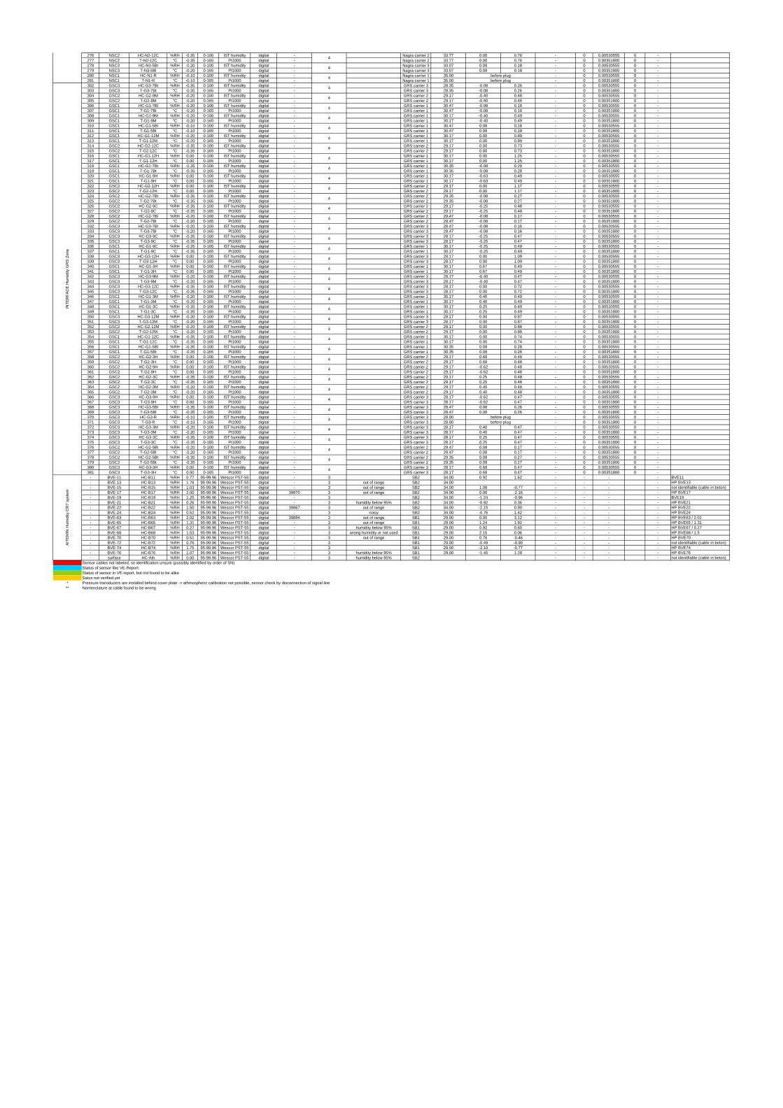
276 NSC2 HC-N2-12C %RH -0.35 0-100 IST humidity digital - Nagra carrier 2 33.77 0.00 0.76 - 0 0.00530555 0 -277 NSC2 T-N2-12C °C -0.35 0-165 Pt1000 digital - Nagra carrier 2 33.77 0.00 0.76 - 0 0.00351800 0 -278 NSC3 HC-N3-5Bl %RH -0.20 0-100 IST humidity digital - Nagra carrier 3 33.07 0.08 0.18 - 0 0.00530555 0 -279 NSC3 T-N3-5Bl °C -0.20 0-165 Pt1000 digital - Nagra carrier 3 33.07 0.08 0.18 - 0 0.00351800 0 -280 NSC1 HC-N1-R %RH -0.10 0-100 IST humidity digital - Nagra carrier 1 35.00 - 0 0.00530555 0 -281 NSC1 T-N1-R °C -0.10 0-165 Pt1000 digital - Nagra carrier 1 35.00 - 0 0.00351800 0 -302 GSC3 HC-G3-7Bt %RH -0.35 0-100 IST humidity digital - GRS carrier 3 28.35 -0.08 0.26 - 0 0.00530555 0 -303 GSC3 T-G3-7Bt °C -0.35 0-165 Pt1000 digital - GRS carrier 3 28.35 -0.08 0.26 - 0 0.00351800 0 -304 GSC2 HC-G2-9M %RH -0.20 0-100 IST humidity digital - GRS carrier 2 29.17 -0.40 0.48 - 0 0.00530555 0 -305 GSC2 T-G2-9M °C -0.20 0-165 Pt1000 digital - GRS carrier 2 29.17 -0.40 0.48 - 0 0.00351800 0 -306 GSC1 HC-G1-7Bl %RH -0.20 0-100 IST humidity digital - GRS carrier 1 30.47 -0.08 0.18 - 0 0.00530555 0 -307 GSC1 T-G1-7Bl °C -0.20 0-165 Pt1000 digital - GRS carrier 1 30.47 -0.08 0.18 - 0 0.00351800 0 -308 GSC1 HC-G1-9M %RH -0.20 0-100 IST humidity digital - GRS carrier 1 30.17 -0.40 0.49 - 0 0.00530555 0 -309 GSC1 T-G1-9M °C -0.20 0-165 Pt1000 digital - GRS carrier 1 30.17 -0.40 0.49 - 0 0.00351800 0 -310 GSC1 HC-G1-5Bl %RH -0.10 0-100 IST humidity digital - GRS carrier 1 30.47 0.08 0.18 - 0 0.00530555 0 -311 GSC1 T-G1-5Bl °C -0.10 0-165 Pt1000 digital - GRS carrier 1 30.47 0.08 0.18 - 0 0.00351800 0 -312 GSC1 HC-G1-12M %RH -0.20 0-100 IST humidity digital - GRS carrier 1 30.17 0.00 0.89 - 0 0.00530555 0 -313 GSC1 T-G1-12M °C -0.20 0-165 Pt1000 digital - GRS carrier 1 30.17 0.00 0.89 - 0 0.00351800 0 -314 GSC2 HC-G2-12C %RH -0.35 0-100 IST humidity digital - GRS carrier 2 29.17 0.00 0.73 - 0 0.00530555 0 -315 GSC2 T-G2-12C °C -0.35 0-165 Pt1000 digital - GRS carrier 2 29.17 0.00 0.73 - 0 0.00351800 0 -316 GSC1 HC-G1-12H %RH 0.00 0-100 IST humidity digital - GRS carrier 1 30.17 0.00 1.25 - 0 0.00530555 0 -317 GSC1 T-G1-12H °C 0.00 0-165 Pt1000 digital - GRS carrier 1 30.17 0.00 1.25 - 0 0.00351800 0 -318 GSC1 HC-G1-7Bt %RH -0.35 0-100 IST humidity digital - GRS carrier 1 30.35 -0.08 0.28 - 0 0.00530555 0 -319 GSC1 T-G1-7Bt °C -0.35 0-165 Pt1000 digital - GRS carrier 1 30.35 -0.08 0.28 - 0 0.00351800 0 -320 GSC1 HC-G1-9H %RH 0.00 0-100 IST humidity digital - GRS carrier 1 30.17 -0.63 0.49 - 0 0.00530555 0 -321 GSC1 T-G1-9H °C 0.00 0-165 Pt1000 digital - GRS carrier 1 30.17 -0.63 0.49 - 0 0.00351800 0 -322 GSC2 HC-G2-12H %RH 0.00 0-100 IST humidity digital - GRS carrier 2 29.17 0.00 1.17 - 0 0.00530555 0 -323 GSC2 T-G2-12H °C 0.00 0-165 Pt1000 digital - GRS carrier 2 29.17 0.00 1.17 - 0 0.00351800 0 -324 GSC2 HC-G2-7Bt %RH -0.35 0-100 IST humidity digital - GRS carrier 2 29.35 -0.08 0.27 - 0 0.00530555 0 -325 GSC2 T-G2-7Bt °C -0.35 0-165 Pt1000 digital - GRS carrier 2 29.35 -0.08 0.27 - 0 0.00351800 0 -326 GSC2 HC-G2-9C %RH -0.35 0-100 IST humidity digital - GRS carrier 2 29.17 -0.25 0.48 - 0 0.00530555 0 -327 GSC2 T-G2-9C °C -0.35 0-165 Pt1000 digital - GRS carrier 2 29.17 -0.25 0.48 - 0 0.00351800 0 -328 GSC2 HC-G2-7Bl %RH -0.20 0-100 IST humidity digital - GRS carrier 2 29.47 -0.08 0.17 - 0 0.00530555 0 -329 GSC2 T-G2-7Bl °C -0.20 0-165 Pt1000 digital - GRS carrier 2 29.47 -0.08 0.17 - 0 0.00351800 0 -332 GSC3 HC-G3-7Bl %RH -0.20 0-100 IST humidity digital - GRS carrier 3 28.47 -0.08 0.16 - 0 0.00530555 0 -333 GSC3 T-G3-7Bl °C -0.20 0-165 Pt1000 digital - GRS carrier 3 28.47 -0.08 0.16 - 0 0.00351800 0 -334 GSC3 HC-G3-9C %RH -0.35 0-100 IST humidity digital - GRS carrier 3 28.17 -0.25 0.47 - 0 0.00530555 0 -335 GSC3 T-G3-9C °C -0.35 0-165 Pt1000 digital - GRS carrier 3 28.17 -0.25 0.47 - 0 0.00351800 0 -336 GSC1 HC-G1-9C %RH -0.35 0-100 IST humidity digital - GRS carrier 1 30.17 -0.25 0.49 - 0 0.00530555 0 -337 GSC1 T-G1-9C °C -0.35 0-165 Pt1000 digital - GRS carrier 1 30.17 -0.25 0.49 - 0 0.00351800 0 -338 GSC3 HC-G3-12H %RH 0.00 0-100 IST humidity digital - GRS carrier 3 28.17 0.00 1.09 - 0 0.00530555 0 -339 GSC3 T-G3-12H °C 0.00 0-165 Pt1000 digital - GRS carrier 3 28.17 0.00 1.09 - 0 0.00351800 0 -340 GSC1 HC-G1-3H %RH 0.00 0-100 IST humidity digital - GRS carrier 1 30.17 0.67 0.49 - 0 0.00530555 0 -341 GSC1 T-G1-3H °C 0.00 0-165 Pt1000 digital - GRS carrier 1 30.17 0.67 0.49 - 0 0.00351800 0 -342 GSC3 HC-G3-9M %RH -0.20 0-100 IST humidity digital - GRS carrier 3 28.17 -0.40 0.47 - 0 0.00530555 0 -343 GSC3 T-G3-9M °C -0.20 0-165 Pt1000 digital - GRS carrier 3 28.17 -0.40 0.47 - 0 0.00351800 0 -344 GSC3 HC-G3-12C %RH -0.35 0-100 IST humidity digital - GRS carrier 3 28.17 0.00 0.72 - 0 0.00530555 0 -345 GSC3 T-G3-12C °C -0.35 0-165 Pt1000 digital - GRS carrier 3 28.17 0.00 0.72 - 0 0.00351800 0 -346 GSC1 HC-G1-3M %RH -0.20 0-100 IST humidity digital - GRS carrier 1 30.17 0.40 0.49 - 0 0.00530555 0 -347 GSC1 T-G1-3M °C -0.20 0-165 Pt1000 digital - GRS carrier 1 30.17 0.40 0.49 - 0 0.00351800 0 -348 GSC1 HC-G1-3C %RH -0.35 0-100 IST humidity digital - GRS carrier 1 30.17 0.25 0.49 - 0 0.00530555 0 -349 GSC1 T-G1-3C °C -0.35 0-165 Pt1000 digital - GRS carrier 1 30.17 0.25 0.49 - 0 0.00351800 0 -350 GSC3 HC-G3-12M %RH -0.20 0-100 IST humidity digital - GRS carrier 3 28.17 0.00 0.87 - 0 0.00530555 0 -351 GSC3 T-G3-12M °C -0.20 0-165 Pt1000 digital - GRS carrier 3 28.17 0.00 0.87 - 0 0.00351800 0 -352 GSC2 HC-G2-12M %RH -0.20 0-100 IST humidity digital - GRS carrier 2 29.17 0.00 0.88 - 0 0.00530555 0 -353 GSC2 T-G2-12M °C -0.20 0-165 Pt1000 digital - GRS carrier 2 29.17 0.00 0.88 - 0 0.00351800 0 -354 GSC1 HC-G1-12C %RH -0.35 0-100 IST humidity digital - GRS carrier 1 30.17 0.00 0.74 - 0 0.00530555 0 -355 GSC1 T-G1-12C °C -0.35 0-165 Pt1000 digital - GRS carrier 1 30.17 0.00 0.74 - 0 0.00351800 0 -356 GSC1 HC-G1-5Bt %RH -0.35 0-100 IST humidity digital - GRS carrier 1 30.35 0.08 0.28 - 0 0.00530555 0 -357 GSC1 T-G1-5Bt °C -0.35 0-165 Pt1000 digital - GRS carrier 1 30.35 0.08 0.28 - 0 0.00351800 0 -358 GSC2 HC-G2-3H %RH 0.00 0-100 IST humidity digital - GRS carrier 2 29.17 0.68 0.48 - 0 0.00530555 0 -359 GSC2 T-G2-3H °C 0.00 0-165 Pt1000 digital - GRS carrier 2 29.17 0.68 0.48 - 0 0.00351800 0 -360 GSC2 HC-G2-9H %RH 0.00 0-100 IST humidity digital - GRS carrier 2 29.17 -0.62 0.48 - 0 0.00530555 0 -361 GSC2 T-G2-9H °C 0.00 0-165 Pt1000 digital - GRS carrier 2 29.17 -0.62 0.48 - 0 0.00351800 0 -362 GSC2 HC-G2-3C %RH -0.35 0-100 IST humidity digital - GRS carrier 2 29.17 0.25 0.48 - 0 0.00530555 0 -363 GSC2 T-G2-3C °C -0.35 0-165 Pt1000 digital - GRS carrier 2 29.17 0.25 0.48 - 0 0.00351800 0 -364 GSC2 HC-G2-3M %RH -0.20 0-100 IST humidity digital - GRS carrier 2 29.17 0.40 0.48 - 0 0.00530555 0 -365 GSC2 T-G2-3M °C -0.20 0-165 Pt1000 digital - GRS carrier 2 29.17 0.40 0.48 - 0 0.00351800 0 -366 GSC3 HC-G3-9H %RH 0.00 0-100 IST humidity digital - GRS carrier 3 28.17 -0.62 0.47 - 0 0.00530555 0 -367 GSC3 T-G3-9H °C 0.00 0-165 Pt1000 digital - GRS carrier 3 28.17 -0.62 0.47 - 0 0.00351800 0 -368 GSC3 HC-G3-5Bl %RH -0.35 0-100 IST humidity digital - GRS carrier 3 28.47 0.08 0.26 - 0 0.00530555 0 -369 GSC3 T-G3-5Bl °C -0.35 0-165 Pt1000 digital - GRS carrier 3 28.47 0.08 0.26 - 0 0.00351800 0 -370 GSC3 HC-G3-R %RH -0.10 0-100 IST humidity digital - GRS carrier 3 28.00 - 0 0.00530555 0 -371 GSC3 T-G3-R °C -0.10 0-165 Pt1000 digital - GRS carrier 3 28.00 - 0 0.00351800 0 -372 GSC3 HC-G3-3M %RH -0.20 0-100 IST humidity digital - GRS carrier 3 28.17 0.40 0.47 - 0 0.00530555 0 -373 GSC3 T-G3-3M °C -0.20 0-165 Pt1000 digital - GRS carrier 3 28.17 0.40 0.47 - 0 0.00351800 0 -374 GSC3 HC-G3-3C %RH -0.35 0-100 IST humidity digital - GRS carrier 3 28.17 0.25 0.47 - 0 0.00530555 0 -375 GSC3 T-G3-3C °C -0.35 0-165 Pt1000 digital - GRS carrier 3 28.17 0.25 0.47 - 0 0.00351800 0 -376 GSC2 HC-G2-5Bl %RH -0.20 0-100 IST humidity digital - GRS carrier 2 29.47 0.08 0.17 - 0 0.00530555 0 -377 GSC2 T-G2-5Bl °C -0.20 0-165 Pt1000 digital - GRS carrier 2 29.47 0.08 0.17 - 0 0.00351800 0 -378 GSC2 HC-G2-5Bt %RH -0.35 0-100 IST humidity digital - GRS carrier 2 29.35 0.08 0.27 - 0 0.00530555 0 -379 GSC2 T-G2-5Bt °C -0.35 0-165 Pt1000 digital - GRS carrier 2 29.35 0.08 0.27 - 0 0.00351800 0 -380 GSC3 HC-G3-3H %RH 0.00 0-100 IST humidity digital - GRS carrier 3 28.17 0.68 0.47 - 0 0.00530555 0 -381 GSC3 T-G3-3H °C 0.00 0-165 Pt1000 digital - GRS carrier 3 28.17 0.68 0.47 - 0 0.00351800 0 -
- BVE-11 HC-B11 %RH 0.77 95-99.96 Wescor PST-55 digital - 3 SB2 34.00 0.92 1.62 - - - - BVE11- BVE-13 HC-B13 %RH 1.76 95-99.96 Wescor PST-55 digital - 3 out of range SB2 34.00 - - - - HP BVE13- BVE-15 HC-B15 %RH 1.03 95-99.96 Wescor PST-55 digital - 3 out of range SB2 34.00 1.08 -0.77 - - - - not identifiable (cable in beton)- BVE-17 HC-B17 %RH 2.00 95-99.96 Wescor PST-55 digital 39870 3 out of range SB2 34.00 0.00 -2.16 - - - - HP BVE17- BVE-19 HC-B19 %RH 1.25 95-99.96 Wescor PST-55 digital - 3 SB2 34.00 -1.24 -0.96 - - - - BVE19- BVE-21 HC-B21 %RH 0.26 95-99.96 Wescor PST-55 digital - 3 humidity below 95% SB2 34.00 -0.92 0.36 - - - - HP BVE21- BVE-22 HC-B22 %RH 1.50 95-99.96 Wescor PST-55 digital 39867 3 out of range SB2 34.00 -2.15 0.90 - - - - HP BVE22- BVE-24 HC-B24 %RH 0.52 95-99.96 Wescor PST-55 digital - 3 noisy SB2 34.00 -0.76 1.42 - - - - HP BVE24- BVE-63 HC-B63 %RH 2.02 95-99.96 Wescor PST-55 digital 39884 3 out of range SB1 29.00 0.00 3.12 - - - - HP BVE63 / 2.01- BVE-65 HC-B65 %RH 1.31 95-99.96 Wescor PST-55 digital - 3 out of range SB1 29.00 1.24 1.92 - - - - HP BVE65 / 1.31- BVE-67 HC-B67 %RH 0.27 95-99.96 Wescor PST-55 digital - 3 humidity below 95% SB1 29.00 0.92 0.60 - - - - HP BVE67 / 0.27- BVE-68 HC-B68 %RH 1.53 95-99.96 Wescor PST-55 digital - 3 wrong humidity or not used SB1 29.00 2.15 0.06 - - - - HP BVE68 / 1.5- BVE-70 HC-B70 %RH 0.51 95-99.96 Wescor PST-55 digital - 3 out of range SB1 29.00 0.76 -0.46 - - - - HP BVE70- BVE-72 HC-B72 %RH 0.76 95-99.96 Wescor PST-55 digital - 3 SB1 29.00 -0.49 -0.90 - - - - not identifiable (cable in beton)- BVE-74 HC-B74 %RH 1.75 95-99.96 Wescor PST-55 digital - 3 SB1 29.00 -2.10 -0.77 - - - - HP BVE74- BVE-76 HC-B76 %RH 1.07 95-99.96 Wescor PST-55 digital - 3 humidity below 95% SB1 29.00 -1.45 1.28 - - - - HP BVE76- surface HC-Ath %RH 0.00 95-99.96 Wescor PST-55 digital - 3 humidity below 95% SB2 - - - - not identifiable (cable in beton)
Sensor cables not labeled, so identification unsure (possibly identified by order of SN)Status of sensor like VE-ReportStatus of sensor in VE-report, but not found to be alikeSatus not verified yet
*** Nomenclature at cable found to be wrong
4
4
4
4
4
4
INT
ER
FA
CE
Hum
idity
GR
S Z
one
4
4
4
4
4
4
4
4
4
4
4
4
4
4
4
4
4
4
before plugbefore plug
before plugbefore plug
4
4
AIT
EM
IN H
umid
ity C
R7
syst
em
Pressure transducers are installed behind cover plate -> athmospheric calibration not possible, sensor check by disconnection of signal line
4
4
4
4
4
4
4
4
4
4
4
4
4
4
4
4

Appendix 4 / D-1 NAGRA NAB 11-25
Appendix 4 Laboratory tests of emplaced bentonite materials

Nagra Hardstrasse 73 CH-5430 Wettingen Dr. Sven Köhler
PEBS ------------------------------------------------------------------------------
Laboratory tests on bentonite
------------------------------------------------------------------------------
IGT Report CL1000, Nagra 9739 1. September 2011
Appendix 4 / D-2 NAGRA NAB 11-25

1
Content:
1. Introduction 2 2. Sampling 2
3. Methods 2
4. Results 4
5. Summary 5
Appendix 1: Photo documentation sampling
Appendix 2: Data tables
Appendix 4 / D-3 NAGRA NAB 11-25

2
1 Introduction
The main aim of the PEBS (Long-term Performance of the Engineered Barrier System) project is to evaluate the sealing and barrier performance of the EBS over time. The bentonite buffer around the canister in nuclear waste disposal involves a foundation of the canister made from highly compacted bentonite blocks and granular material. NAGRA assigned the Institute of Geotechnical Engineering of the ETH Zurich (IGT) with the analysis of a bentonite block made from MX-80 (IGT Report 4771 and additional in the present report) and samples from granular bentonite material concerning different densities, water content and grain size distribution.
2 Sampling
The samples were delivered on 29. April 2011 in plastic containers. Samples consist in fragments of different bentonite blocks (1-3) made from MX-80 and granular material from Bigbag A and E sampled on different days.
Sample description remarks
Block 1 Fragments from block 1 Analyse of two pieces each
Block 2 Fragments from block 1 Analyse of two pieces each
Block 3 Fragments from block 1 Analyse of two pieces each
S1-5 5 containers sampled on 6. and 7. April from Bigbag E
Analyse of a representative composite sample
S6-10 5 containers sampled on 7. and 8. April from Bigbag E
Analyse of a representative composite sample
S11-14 4 containers sampled on 11. and 12. April from Bigbag A
Analyse of a representative composite sample
S15-20 6 containers sampled on 11. and 12. April from Bigbag E
Analyse of a representative composite sample
Appendix 4 / D-4 NAGRA NAB 11-25
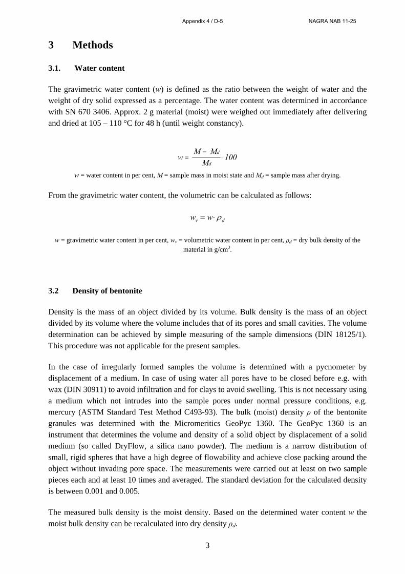
3
3 Methods
3.1. Water content
The gravimetric water content (w) is defined as the ratio between the weight of water and the weight of dry solid expressed as a percentage. The water content was determined in accordance with SN 670 3406. Approx. 2 g material (moist) were weighed out immediately after delivering and dried at 105 – 110 °C for 48 h (until weight constancy).
w = water content in per cent, M = sample mass in moist state and Md = sample mass after drying.
From the gravimetric water content, the volumetric can be calculated as follows:
dv ww
w = gravimetric water content in per cent, wv = volumetric water content in per cent, ρd = dry bulk density of the material in g/cm3.
3.2 Density of bentonite
Density is the mass of an object divided by its volume. Bulk density is the mass of an object divided by its volume where the volume includes that of its pores and small cavities. The volume determination can be achieved by simple measuring of the sample dimensions (DIN 18125/1). This procedure was not applicable for the present samples.
In the case of irregularly formed samples the volume is determined with a pycnometer by displacement of a medium. In case of using water all pores have to be closed before e.g. with wax (DIN 30911) to avoid infiltration and for clays to avoid swelling. This is not necessary using a medium which not intrudes into the sample pores under normal pressure conditions, e.g. mercury (ASTM Standard Test Method C493-93). The bulk (moist) density ρ of the bentonite granules was determined with the Micromeritics GeoPyc 1360. The GeoPyc 1360 is an instrument that determines the volume and density of a solid object by displacement of a solid medium (so called DryFlow, a silica nano powder). The medium is a narrow distribution of small, rigid spheres that have a high degree of flowability and achieve close packing around the object without invading pore space. The measurements were carried out at least on two sample pieces each and at least 10 times and averaged. The standard deviation for the calculated density is between 0.001 and 0.005.
The measured bulk density is the moist density. Based on the determined water content w the moist bulk density can be recalculated into dry density ρd.
wM M
M100
d
d
Appendix 4 / D-5 NAGRA NAB 11-25
4
ρd = dry density in g/cm3 (or kg/l), ρ = moist density in g/cm3 and w = water content in per cent.
3.3. Minimal and maximal emplacement density
The emplacement densities of the bentonite material were determined with different procedures (SN 670 335a, DIN 18126, ASTM D 4253-93). The measurement principle is based on filling a cylinder with a diameter of approx. the eightfold of the maximum particle size. A cylinder with a diameter of 5 cm and a volume of 500 cm3 with a 5 ml scale was used. About 740 g material was filled in from a defined height of 10 cm through a funnel to exact 500 mL. After the filling the exact weight fitted in the cylinder was measured. Afterwards, to determine the maximum density m, the filled cylinder was vibrated on a sieve shaker table (amplitude 70, time 2 min until there was no more volume change) and the volume was determined. The measurements were carried out in duplicates and averaged. The density variation is ±0.015 g/mL.
3.4. Grain size distribution (sieve analysis) For the determination of the particle size distribution 1000 g of the material were dry sieved. Sieving was executed with a sieve shaker AS200 (amplitude 70, time 10 min) (RETSCH) and sieves of 8 mm, 5 mm, 2 mm, 1.4 mm, 1 mm, 0.5 mm, 0.25 mm, 0.125 mm, and 0.063 mm opening (high-grade steel of mesh sieves acc. DIN 4188 or DIN ISO 3310/1). The value Q3 gives the amount passing (mesh minus) and the value p3 the residual amount (mesh plus). The analysis was carried out in duplicates and averaged. The evaluation of particle size distribution permits various conclusions on the compaction behaviour. Thus, the distortion number of CU and the curvature number of CC from the particle size distribution are computed. The distortion number of CU represents thereby the relationship of the values for to the grain diameters at 10% and 60% sieve passage.
CU = d60/d10 Values below five show the predomination of a certain grain size (poorly graded), whereas values above are typical for well-graded materials. Since with the computation by CU a large grain range is not considered, one computes the curvature number CC.
CC = (d30)2 / d60
. d10
d 1
w
100
Appendix 4 / D-6 NAGRA NAB 11-25
5
Well-graded material shows good compaction behaviour. The parameters for the ideal, so-called Fuller curve are CU = 36 and CC = 2.25.
3.5. Long-term storage of bentonite blocks at different relative humidity Three cores were drilled (dry) out from the bentonite block made from MX-80 (IGT-Report 4771). These cores were nearly identical from dimension and weight (between 336 g and 338 g, diameter 45 mm and length 100 mm). One each of these cores were stored for 6 months at different relative humidity (open under ambient conditions 50-60% r.H., 75% r.H. and close to 100% r.H.). The 75% r.H. was established in a close, tight container with a saturated NaCl-solution and the 100% by storing in a similar container above an open water surface. The relative humidity and the changes in weight were monitored. 4 Results
Water content and densities
The values of the measurements are given in appendix 1.
The gravimetric water content of the block samples varies between 13.6 and 19.1 wt%. The water content of the granular material is low and almost the same for all samples between 5.9 and 6.0 wt%. According to the different water content different values for the bulk density of the block samples and the granular material can be stated. The block samples lies in the range 1.81 - 1.94 g/cm3. The pellets from the granular material shows higher values in the range 2.01 - 2.18 g/cm3.
In the values of the minimal and maximal emplacement density are the different granular samples from different bigbags and taken at different times almost identical. The minimal emplacement density is in the range 1.47 – 1.49 g/cm3 and the maximal emplacement density in the range 1.68 – 1.70 g/cm3.
Sieve analysis
The sieve curves are given in appendix 2.
The parameters of the sieving analyses shows very similar values for the different samples from bigbag E. The d10 value is 0.05 mm, the d30 between 0.46 and 0.51 mm, the d50 between 1.10 and 1.13 mm, the d60 between 1.55 and 1.62 mm and the d90 between 4.64 and 4.95 mm. The bigbag A shows slightly coarser grains: d30 = 0.68 mm, d50 = 1.64 mm and d60 = 2.46 mm. The averaged sieve curve of the samples from bigbag E with the averaged from mixture E from
Appendix 4 / D-7 NAGRA NAB 11-25
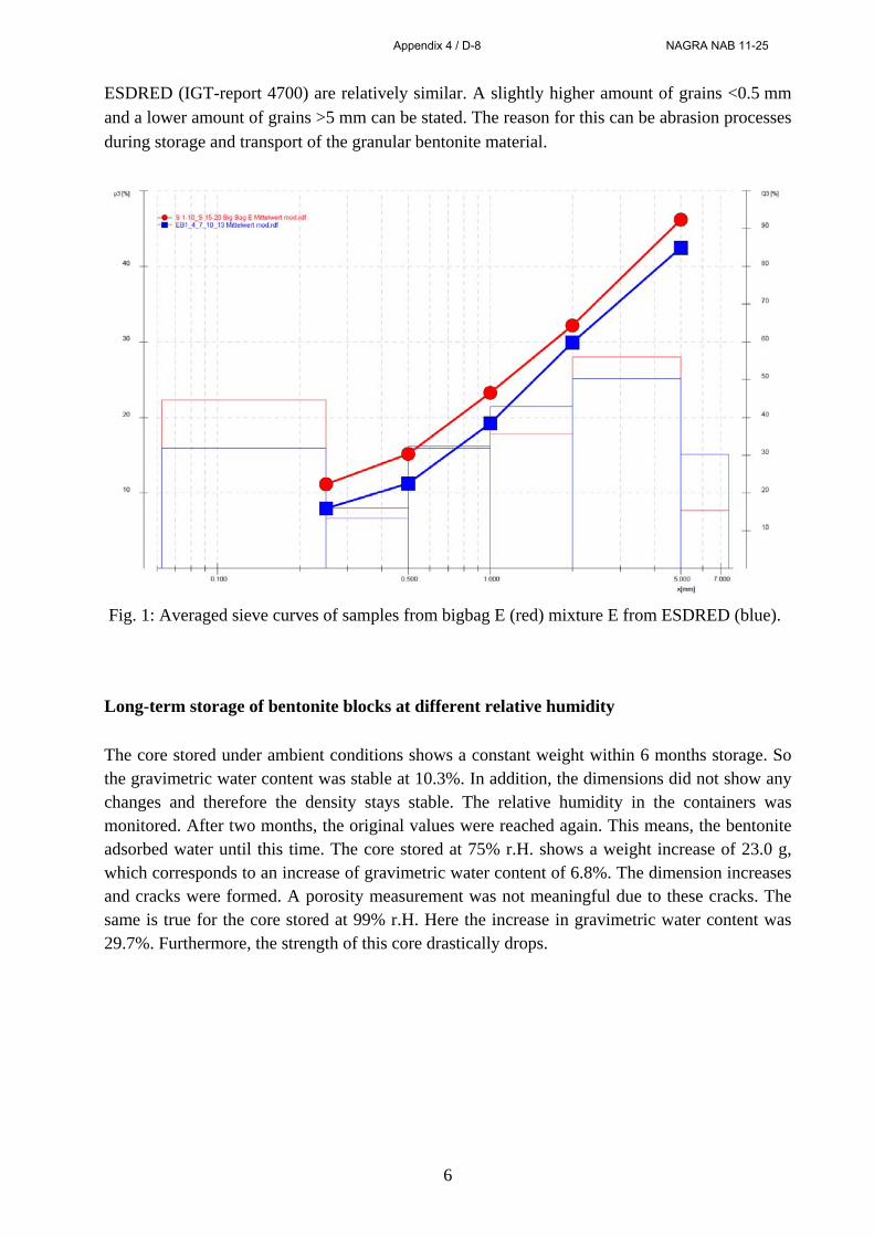
6
ESDRED (IGT-report 4700) are relatively similar. A slightly higher amount of grains <0.5 mm and a lower amount of grains >5 mm can be stated. The reason for this can be abrasion processes during storage and transport of the granular bentonite material.
Fig. 1: Averaged sieve curves of samples from bigbag E (red) mixture E from ESDRED (blue).
Long-term storage of bentonite blocks at different relative humidity
The core stored under ambient conditions shows a constant weight within 6 months storage. So the gravimetric water content was stable at 10.3%. In addition, the dimensions did not show any changes and therefore the density stays stable. The relative humidity in the containers was monitored. After two months, the original values were reached again. This means, the bentonite adsorbed water until this time. The core stored at 75% r.H. shows a weight increase of 23.0 g, which corresponds to an increase of gravimetric water content of 6.8%. The dimension increases and cracks were formed. A porosity measurement was not meaningful due to these cracks. The same is true for the core stored at 99% r.H. Here the increase in gravimetric water content was 29.7%. Furthermore, the strength of this core drastically drops.
Appendix 4 / D-8 NAGRA NAB 11-25
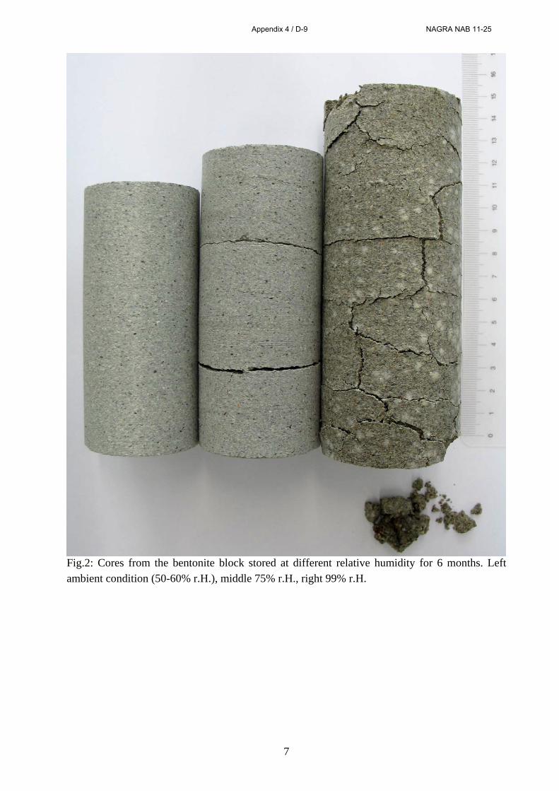
7
Fig.2: Cores from the bentonite block stored at different relative humidity for 6 months. Left ambient condition (50-60% r.H.), middle 75% r.H., right 99% r.H.
Appendix 4 / D-9 NAGRA NAB 11-25
8
5 Summary
In conclusion, the following can be stated: The block samples already adsorbed some water, which leads to higher water content as the original blocks (10 vs. 16%), and slightly lower bulk density (1.99 vs. 1.87 g/cm3). The samples from the granular material are still very dry with water content around 6% and a grain bulk density above 2 g/cm3. With the granular material a maximum emplacement density of 1.7 g/cm3 could be reached.
Storing the bentonite blocks for two months or more at ambient conditions with a relative humidity of 50-60% seems to be without influence on the water content and density. Only at higher relative humidity (75% or more) a drastic increase of water content with a related drastic decrease in density and mechanical strength.
Report Nr. CL1000/MP
Zurich, 1st September 2011
ETH Zurich
Institute for Geotechnical Engineering (IGT)
Dr. M. Plötze
Appendix 4 / D-10 NAGRA NAB 11-25
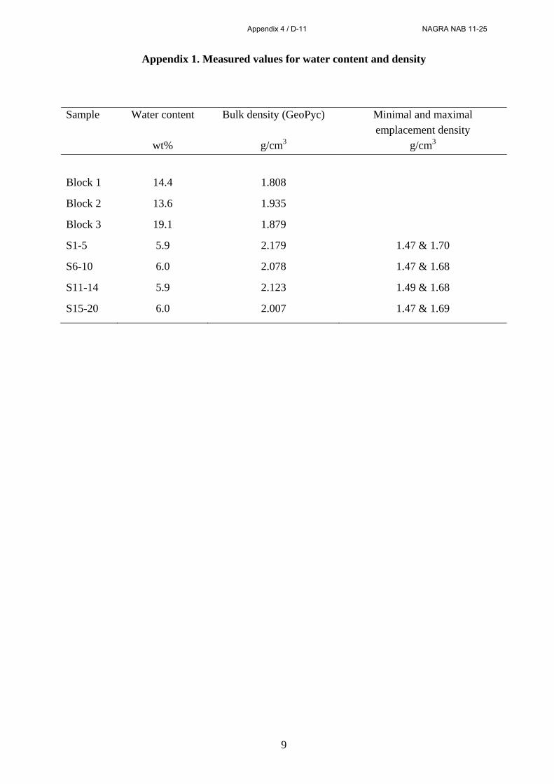
9
Appendix 1. Measured values for water content and density
Sample Water content
wt%
Bulk density (GeoPyc)
g/cm3
Minimal and maximal emplacement density
g/cm3
Block 1 14.4 1.808
Block 2 13.6 1.935
Block 3 19.1 1.879
S1-5 5.9 2.179 1.47 & 1.70
S6-10 6.0 2.078 1.47 & 1.68
S11-14 5.9 2.123 1.49 & 1.68
S15-20 6.0 2.007 1.47 & 1.69
Appendix 4 / D-11 NAGRA NAB 11-25
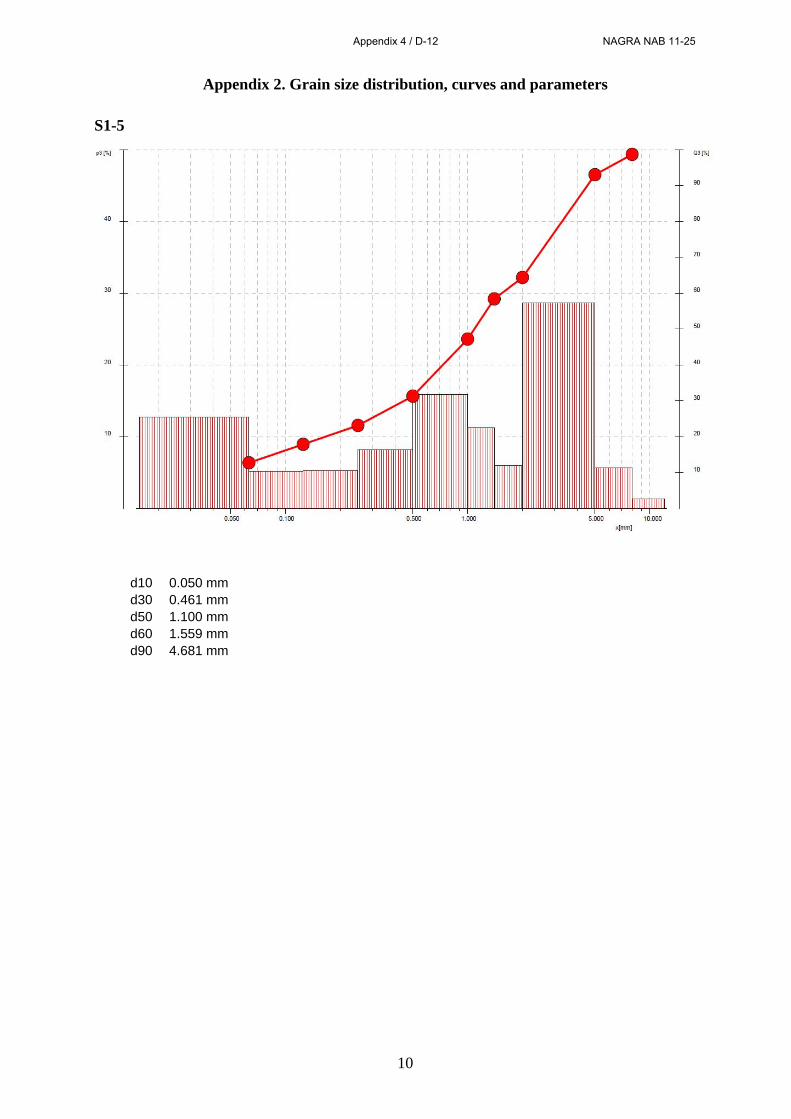
10
Appendix 2. Grain size distribution, curves and parameters
S1-5
d10 0.050 mm d30 0.461 mm d50 1.100 mm d60 1.559 mm d90 4.681 mm
Appendix 4 / D-12 NAGRA NAB 11-25
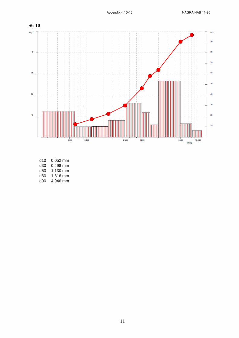
11
S6-10
d10 0.052 mm d30 0.498 mm d50 1.130 mm d60 1.616 mm d90 4.946 mm
Appendix 4 / D-13 NAGRA NAB 11-25
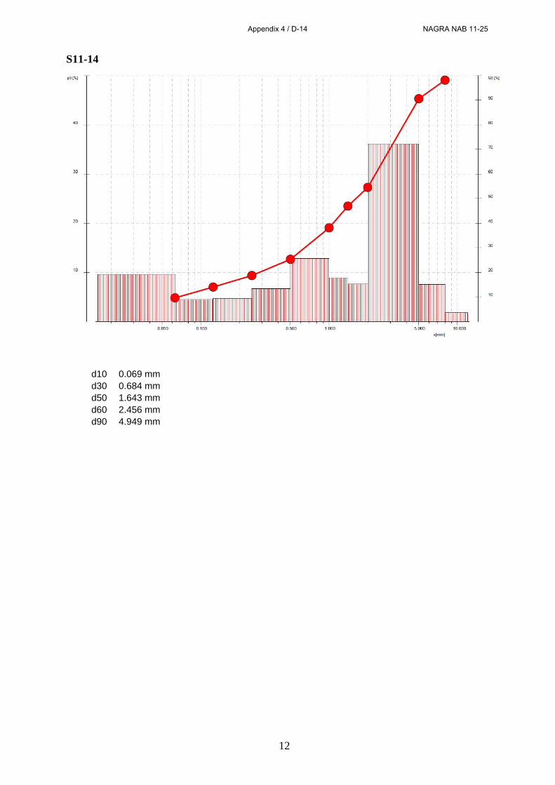
12
S11-14
d10 0.069 mm d30 0.684 mm d50 1.643 mm d60 2.456 mm d90 4.949 mm
Appendix 4 / D-14 NAGRA NAB 11-25
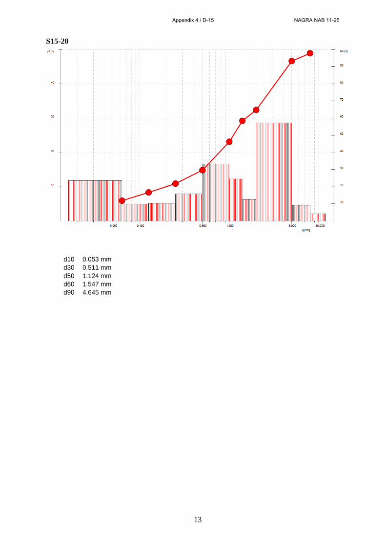
13
S15-20
d10 0.053 mm d30 0.511 mm d50 1.124 mm d60 1.547 mm d90 4.645 mm
Appendix 4 / D-15 NAGRA NAB 11-25
Related Documents